Embed Size (px)
Citation preview

1
INSTITUTE OF AERONAUTICAL ENGINEERING (Autonomous)
Dundigal,Hyderabad-500043
CIVIL ENGINEERING
COURSE LECTURE NOTES
Course Name MATHEMATICAL TRANSFORM TECHNIQUES
Course Code AHSB11
Programme B.Tech
Semester II
Course
Coordinator Dr. S. Jagadha, Associate Professor
Course Faculty Dr. P. Srilatha, Associate Professor
Ms. L Indira, Assistant Professor
Ms. C Rachana, Assistant Professor
Ms. P Rajani, Assistant Professor
Ms. B. Praveena, Assistant Professor
Lecture Numbers 1-63
Topic Covered All
COURSE OBJECTIVES (COs):
The course should enable the students to:
I Enrich the knowledge of solving Algebraic and Transcendental equations and
Differential equation by numerical methods.
II Determine the Fourier transforms for various functions in a given period.
III Determine the Laplace and Inverse Laplace transforms for various functions using
standard types.
IV Formulate to solve Partial differential equation.
COURSE LEARNING OUTCOMES (CLOs):
Students, who complete the course, will have demonstrated the ability to do the following:
AHSB11.01 Evaluate the real roots of algebraic and transcendental equations by Bisection method, False
position and Newton -Raphson method.
AHSB11.02 Apply the nature of properties to Laplace transform and inverse Laplace transform of the
given function.
AHSB11.03 Solving Laplace transforms of a given function using shifting theorems.
AHSB11.04 Evaluate Laplace transforms using derivatives of a given function.
AHSB11.05 Evaluate Laplace transforms using multiplication of a variable to a given function.
AHSB11.06 Apply Laplace transforms to periodic functions.
AHSB11.07 Apply the symbolic relationship between the operators using finite differences.
AHSB11.08 Apply the Newtons forward and Backward, Gauss forward and backward Interpolation
2
method to determine the desired values of the given data at equal intervals, also unequal
intervals.
AHSB11.09 Solving Laplace transforms and inverse Laplace transform using derivatives and integrals.
AHSB11.10 Evaluate inverse of Laplace transforms and inverse Laplace transform by the method of
convolution.
AHSB11.11 Solving the linear differential equations using Laplace transform.
AHSB11.12 Understand the concept of Laplace transforms to the real-world problems of electrical circuits,
harmonic oscillators, optical devices, and mechanical systems
AHSB11.13 Ability to curve fit data using several linear and non linear curves by method of least squares.
AHSB11.14 Understand the nature of the Fourier integral.
AHSB11.15 Ability to compute the Fourier transforms of the given function.
AHSB11.16 Ability to compute the Fourier sine and cosine transforms of the function
AHSB11.17 Evaluate the inverse Fourier transform, Fourier sine and cosine transform of the given
function.
AHSB11.18 Evaluate finite and infinite Fourier transforms
AHSB11.19 Understand the concept of Fourier transforms to the real-world problems of circuit analysis,
control system design
AHSB11.20 Apply numerical methods to obtain approximate solutions to Taylors, Eulers, Modified Eulers
AHSB11.21 Runge-Kutta methods of ordinary differential equations.
AHSB11.22 Understand the concept of order and degree with reference to partial differential equation
AHSB11.23 Formulate and solve partial differential equations by elimination of arbitrary constants and
functions
AHSB11.24 Understand partial differential equation for solving linear equations by Lagrange method.
AHSB11.25 Apply the partial differential equation for solving non-linear equations by Charpit‟s method
AHSB11.26 Apply method of separation of variables, Solving the heat equation and wave equation in
subject to boundary conditions
AHSB11.27 Understand the concept of partial differential equations to the real-world problems of
electromagnetic and fluid dynamics
SYLLABUS
Module-I ROOT FINDING TECHNIQUES AND LAPLACE TRANSFORMS Classes: 09
ROOT FINDING TECHNIQUES:Root finding techniques: Solving algebraic and Transcendental
equations by bisection method, Method of false position, Newton-Raphson method.
LAPLACE TRANSFORMS:Definition of Laplace transform, Linearity property, Piecewise continuous
function, existence of Laplace transform, Function of exponential order, First and second shifting
theorems, change of scale property, Laplace transforms of derivatives and integrals, Multiplied by t,
Divided by t, Laplace transform of periodic functions.
Module-II INTERPOLATION AND INVERSE LAPLACE TRANSFORMS Classes: 09
INTERPOLATION:Interpolation: Finite differences, Forward differences, Backward differences and
central differences; Symbolic relations; Newton‟s forward interpolation, Newton‟s backward
interpolation; Gauss forward central difference formula, Gauss backward central difference formula;
Interpolation of unequal intervals: Lagrange‟s interpolation.
INVERSE LAPLACE TRANSFORMS:Inverse Laplace transform: Definition of Inverse Laplace
transform, Linearity property, First and second shifting theorems, Change of scale property, Multiplied by

3
s, divided by s; Convolution theorem and applications.
Module-III CURVE FITTING AND FOURIER TRANSFORMS Classes: 09
CURVE FITTING: Fitting a straight line; Second degree curves; Exponential curve, Power curve by
method of least squares.
FOURIERTRANSFORMS:Fourier integral theorem, Fourier sine and cosine integrals; Fourier
transforms; Fourier sine and cosine transform, Properties, Inverse transforms, Finite Fourier transforms.
Module-IV NUMERICAL SOLUTION OF ORDINARY DIFFERENTIAL
EQUATIONS Classes: 09
STEP BY STEP METHOD:Taylor‟s series method; Euler‟s method, Modified Euler‟s method for first
order differential equations.
MULTI STEP METHOD: Runge-Kutta method for first order differential equations.
Module-V PARTIAL DIFFERENTIAL EQUATIONS AND APPLICATIONS Classes: 09
PARTIAL DIFFERENTIAL EQUATIONS: Formation of partial differential equations by elimination
of arbitrary constants and arbitrary functions, Solutions of first order linear equation by Lagrange method
and nonlinear by Charpit method
APPLICATIONS: Method of separation of variables; One dimensional heat and wave equations under
initial and boundary conditions.
Text Books:
1. B.S. Grewal, Higher Engineering Mathematics, Khanna Publishers, 36th Edition, 2010.
2. N.P. Bali and Manish Goyal, A text book of Engineering Mathematics, Laxmi Publications, Reprint,
2008.
3. Ramana B.V., Higher Engineering Mathematics, Tata McGraw Hill New Delhi, 11th Reprint,2010.
Reference Books:
1. Erwin Kreyszig, Advanced Engineering Mathematics, 9th Edition, John Wiley & Sons, 2006.
2. Veerarajan T., Engineering Mathematics for first year, Tata McGraw-Hill, New Delhi, 2008.
3. D. Poole, Linear Algebra: A Modern Introduction, 2nd Edition, Brooks/Cole, 2005.
4. Dr. M Anita, Engineering Mathematics-I, Everest Publishing House, Pune, First Edition, 2016.

4
MODULE-I
ROOT FINDING TECHNIQUES AND LAPLACE TRANSFORMS
Solutions of Algebraic and Transcendental equations:
1) Polynomial function: A function f x is said to be a polynomial function
if f x is a polynomial in x.
ie, 𝑓 𝑥 = 𝑎0𝑥𝑛 + 𝑎1𝑥
𝑛−1 + ⋯……… . . +𝑎𝑛−1𝑥 + 𝑎𝑛
where 0 0a , the co-efficients 0 1, ........... na a a are real constants and n is a
non-negative integer.
2) Algebraic function: A function which is a sum (or) difference (or) product of
two polynomials is called an algebraic function. Otherwise, the function is called
a transcendental (or) non-algebraic function.
Eg: 𝑓 𝑥 = 𝑐1𝑒𝑥 + 𝑐2𝑒
−𝑥 = 0
𝑓 𝑥 = 𝑒5𝑥 −𝑥3
2+ 3 = 0
3) Root of an equation: A number is called a root of an equation 0f x if
0f . We also say that is a zero of the function.
Note: The roots of an equation are the abscissae of the points where the graph
y f x cuts the x-axis.
Methods to find the roots of f (x) = 0
Direct method: We know the solution of the polynomial equations such as linear
equation 𝑎𝑥 + 𝑏 =0, and quadratic equation 2 0ax bx c ,using direct methods or
analytical methods. Analytical methods for the solution of cubic and quadratic equations
are also available.
Bisection method: Bisection method is a simple iteration method to solve an equation. This
method is also known as Bolzono method of successive bisection. Some times it is referred to as
half-interval method. Suppose we know an equation of the form 0f x

5
has exactly one real root between two real numbers 0 1,x x .The number is choosen such
that 0f x and 1f x will have opposite sign. Let us bisect the interval 0 1,x x into two
half intervals and find the mid point 0 12
2
x xx
. If 2 0f x then 2x is a root.
If 1f x and 2f x have same sign then the root lies between 0x and x2. The interval is
taken as 𝑥0, 𝑥2 . Otherwise the root lies in the interval 2 1,x x .
PROBLEMS
1). Find a root of the equation 3 5 1 0x x using the bisection method in 5 –
stages
Sol Let 𝑓 𝑥 = 𝑥3 − 5𝑥 + 1. We note that 𝑓 0 > 0
𝑓 1 < 0 𝑎𝑛𝑑
One root lies between 0 and 1
Consider 0 10 1x and x
By Bisection method the next approximation is
0 12
2
10 1 0.5
2 2
0 :5 1.375 0 0 0
x xx
f x f and f
We have the root lies between 0 and 0.5
Now 3
0 0.50.25
2x
We find 3 0.234375 0 0 0f x and f
Since 0 0f , we conclude that root lies between 0 3x and x
The third approximation of the root is
𝑥4 =𝑥0+𝑥3
2=
1
2 0 + 0.25 = 0.125
We have 4 0.37495 0f x
Since 4 30 0f x and f x , the root lies between
4 30.125 0.25x and x

6
Considering the 4th
approximation of the roots
3 45
10.125 0.25 0.1875
2 2
x xx
5 0.06910 0f x , since 5 30 0f x and f x the root must lie
between 𝑥5 = 0.18758 𝑎𝑛𝑑 𝑥3 = 0.25
Here the fifth approximation of the root is
6 5 3
1
2
10.1875 0.25
2
0.21875
x x x
We are asked to do up to 5 stages
We stop here 0.21875 is taken as an approximate value of the root and it
lies between 0 and 1
2) Find a root of the equation 3 4 9 0x x using bisection method in four
stages
Sol Let 3 4 9f x x x
We note that 2 0f and 3 0f
One root lies between 2 and 3
Consider 0 12 3x and x
By Bisection method 0 12 2.5
2
x xx
Calculating 2 2.5 3.375 0f x f
The root lies between 𝑥2 𝑎𝑛𝑑 𝑥1
The second approximation is 𝑥3 =1
2 𝑥1 + 𝑥2 =
2.5+3
2= 2.75
Now 𝑓 𝑥3 = 𝑓 2.75 = 0.7969 > 0
The root lies between 2 3x and x
Thus the third approximation to the root is
4 2 3
12.625
2x x x
7
Again 4 2.625 1.421 0f x f
The root lies between 3 4x and x
Fourth approximation is𝑥5 =1
2 𝑥3 + 𝑥4 =
1
2 2.75 + 2.625 = 2.6875
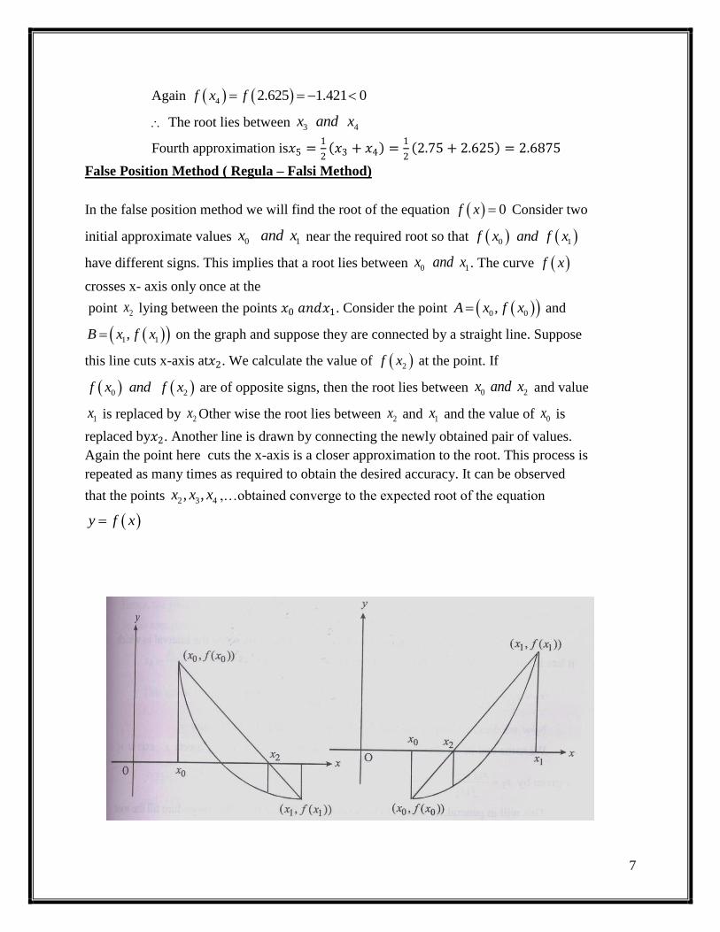
False Position Method ( Regula – Falsi Method)
In the false position method we will find the root of the equation 0f x Consider two
initial approximate values 0 1x and x near the required root so that 0 1f x and f x
have different signs. This implies that a root lies between 0 1x and x . The curve f x
crosses x- axis only once at the
point 2x lying between the points 𝑥0 𝑎𝑛𝑑𝑥1. Consider the point 0 0,A x f x and
1 1,B x f x on the graph and suppose they are connected by a straight line. Suppose
this line cuts x-axis at𝑥2. We calculate the value of 2f x at the point. If
0 2f x and f x are of opposite signs, then the root lies between 0 2x and x and value
1x is replaced by 2x Other wise the root lies between 2x and 1x and the value of 0x is
replaced by𝑥2. Another line is drawn by connecting the newly obtained pair of values.
Again the point here cuts the x-axis is a closer approximation to the root. This process is
repeated as many times as required to obtain the desired accuracy. It can be observed
that the points 2 3 4, ,x x x ,…obtained converge to the expected root of the equation
y f x

8
To Obtain the equation to find the next approximation to the root
Let 0 0 1 1, ,A x f x and B x f x be the points on the curve y f x Then the
equation to the chord AB is 𝑦−𝑓 𝑥0
𝑥−𝑥0=
𝑓 𝑥1 −𝑓 𝑥0
𝑥1−𝑥0− − − − − − 1
At the point C where the line AB crosses the x – axis, where 𝑓 𝑥 = 0 𝑖𝑒, 𝑦 = 0
From (1), we get
1 00 0
1 0
2x x
x x f xf x f x
x is given by (2) serves as an approximated value of the root, when the interval in which it
lies is small. If the new value of x is taken as 2x then (2) becomes
1 0
2 0 0
1 0
0 1 1 0
1 0
3
x xx x f x
f x f x
x f x x f x
f x f x
Now we decide whether the root lies between
0 2 2 1x and x or x and x
We name that interval as 1 2,x x The line joining 𝑥1, 𝑦1 , 𝑥2, 𝑦2 meets x –
axis at 3x is given by
1 2 2 1
3
2 1
x f x x f xx
f x f x
This will in general, be nearest to the exact root. We continue this procedure till
the root is found to the desired accuracy
The iteration process based on (3) is known as the method of false position
The successive intervals where the root lies, in the above procedure are named
as
--------------(2)
-------------(3)

9
0 1 1 2 2 3, , , , ,x x x x x x etc
Where 𝑥𝑖 < 𝑥𝑖+1 and𝑓 𝑥0 , 𝑓 𝑥𝑖+1 are of opposite signs.
Also
1 1
1
1
i i i i
i
i i
x f x x f xx
f x f x
PROBLEMS:
1. By using Regula - Falsi method, find an approximate root of the equation 4 10 0x x that lies between 1.8 and 2. Carry out three approximations
Sol. Let us take 4 10f x x x and 0 11.8, 2x x
Then 0 1.8 1.3 0f x f and 1 2 4 0f x f
Since 0f x and 1f x are of opposite signs,the equation 0f x has a
root between 0 1x and x
The first order approximation of this root is
1 02 0 0
1 0
2 1.81.8 1.3
4 1.3
1.849
x xx x f x
f x f x
We find that 2 0.161f x so that 2 1f x and f x are of opposite signs.
Hence the root lies between 2 1x and x and the second order approximation of
the root is
1 23 2 2
1 2
.
2 1.8491.8490 0.159
0.159
1.8548
x xx x f x
f x f x
we find that 3 1.8548f x f
0.019
So that 3 2f x and f x are of the same sign. Hence, the root does not lie
between 2 3x and x .But 3 1f x and f x are of opposite signs. So the root

10
lies between 3 1x and x and the third order approximate value of the root is
𝑥4 = 𝑥3 − 𝑥1−𝑥3
𝑓 𝑥1 −𝑓 𝑥3 𝑓 𝑥3
= 1.8548 −2 − 1.8548
4 + 0.019× −0.019
= 1.8557
This gives the approximate value of x.
2. Find out the roots of the equation 3 4 0x x using False position method
Sol. Let 3 4 0f x x x
Then 0 4, 1 4, 2 2f f f
Since 1 2f and f have opposite signs the root lies between 1 and 2
By False position method
0 1 1 0
2
1 0
x f x x f xx
f x f x
2
1 2 2 4
2 4
2 8 101.666
6 6
x
31.666 1.666 1.666 4
1.042
f
Now, the root lies between 1.666 and 2
3
3
1.666 2 2 1.0421.780
2 1.042
1.780 1.780 1.780 4
0.1402
x
f
Now, the root lies between 1.780 and 2
4
3
1.780 2 2 0.14021.794
2 0.1402
1.794 1.794 1.794 4
0.0201
x
f
Now, the root lies between 1.794 and 2
11
5
3
1.794 2 2 0.02011.796
2 0.0201
1.796 1.796 1.796 4 0.0027
x
f
Now, the root lies between 1.796 and 2
6
1.796 2 2 0.00271.796
2 0.0027x
The root is 1.796
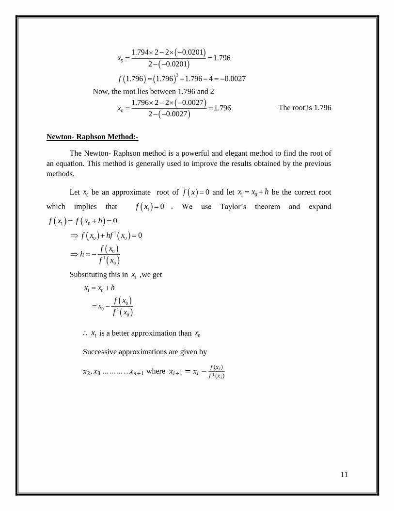
Newton- Raphson Method:-
The Newton- Raphson method is a powerful and elegant method to find the root of
an equation. This method is generally used to improve the results obtained by the previous
methods.
Let 0x be an approximate root of 0f x and let 1 0x x h be the correct root
which implies that 1 0f x . We use Taylor‟s theorem and expand
1 0 0f x f x h
1
0 0
0
1
0
0f x hf x
f xh
f x
Substituting this in 1x ,we get
1 0
0
0 1
0
x x h
f xx
f x
1x is a better approximation than 0x
Successive approximations are given by
𝑥2 , 𝑥3 ……… . . 𝑥𝑛+1 where 𝑥𝑖+1 = 𝑥𝑖 −𝑓 𝑥𝑖
𝑓1(𝑥𝑖)

12
Problems:
1. Apply Newton – Raphson method to find an approximate root, correct to three
decimal places, of the equation 3 3 5 0,x x which lies near 2x
Sol:- Here 3 1 23 5 0 3 1f x x x and f x x
The Newton – Raphson iterative formula
3 3
1 2 2
3 5 2 5, 0,1,2.... 1
3 1 3 1
i i ii i
i i
x x xx x i
x x
To find the root near 2x , we take 0 2x then (1) gives
3
01 2
0
33
12 22
1
2 5 16 5 212.3333
3 4 1 93 1
2 2.3333 52 52.2806
3 1 3 2.3333 1
xx
x
xx
x
𝑥3 =2𝑥2
3 + 5
3 𝑥23 − 1
=2 × 2.2806 3 + 5
3 2.2806 2 − 1 = 2.2790
𝑥4 =2 × 2.2790 3 + 5
3 2.2790 2 − 1 = 2.2790
Since 3x and 4x are identical up to 3 places of decimal, we take 4 2.279x as the
required root, correct to three places of the decimal
LAPLACE TRANSFORMS
Introduction

13
In mathematics the Laplace transform is an integral transform named after its discoverer Pierre-
Simon Laplace . It takes a function of a positive real variable t (often time) to a function of a
complex variable s (frequency).The Laplace transform is very similar to the Fourier transform.
While the Fourier transform of a function is a complex function of a real variable (frequency),
the Laplace transform of a function is a complex function of a complex variable. Laplace
transforms are usually restricted to functions of t with t > 0. A consequence of this restriction is
that the Laplace transform of a function is a holomorphic function of the variable s. Unlike the
Fourier transform, the Laplace transform of a distribution is generally a well-behaved function.
Also techniques of complex variables can be used directly to study Laplace transforms. As a
holomorphic function, the Laplace transform has a power series representation. This power series
expresses a function as a linear superposition of moments of the function. This perspective has
applications in probability theory.
Introduction
Let f(t) be a given function which is defined for all positive values of t, if
F(s) =
0
e-st
f(t) dt
exists, then F(s) is called Laplace transform of f(t) and is denoted by
L{f(t)} = F(s) =
0
e-st
f(t) dt
The inverse transform, or inverse of L{f(t)} or F(s), is
f(t) = L-1
{F(s)}
where s is real or complex value.
14
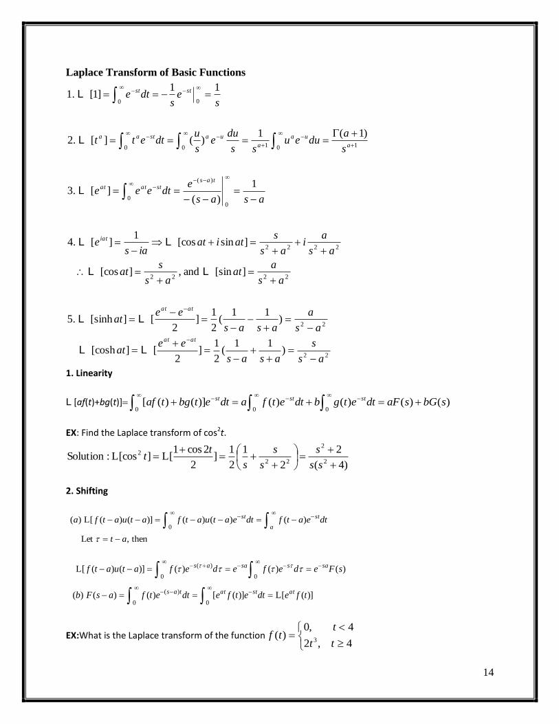
Laplace Transform of Basic Functions
22
22
2222
2222
0
)(
0
10100
00
)11
(2
1]
2[][cosh
)11
(2
1]
2[][sinh.5
][sinand,][cos
]sin[cos1
][.4
1
)(][.3
)1(1)(][.2
11]1[.1
as
s
asas
eeat
as
a
asas
eeat
as
aat
as
sat
as
ai
as
satiat
iase
asas
edteee
s
adueu
ss
due
s
udtett
se
sdte
atat
atat
iat
tasstatat
a
ua
a
uastaa
stst
LL
LL
LL
LL
L
L
L
1. Linearity
L [af(t)+bg(t)] )()()()()]()([000
sbGsaFdtetgbdtetfadtetbgtaf ststst
EX: Find the Laplace transform of cos2t.
)4(
2
2
1
2
1]
2
2cos1[L][cosL:Solution
2
2
22
2
ss
s
s
s
s
tt
2. Shifting
then,Let
)()()()]()([L)(0
at
dteatfdteatuatfatuatfaa
stst
)]([L)]([)()()(
)()()()]()([L
00
)(
00
)(
tfedtetfedtetfasFb
sFedefedefatuatf
atstattas
sassaas
EX:What is the Laplace transform of the function
4,2
4,0)(
3 tt
ttf

15
Solution: f(t)2t3u(t4)
L [f(t)]L {2[(t4)3+12(t4)2+48(t4)+64]u(t4)}
sssse
sssse ss 3224123
4641
48!2
12!3
2234
4
234
4
3. Scaling
)(1
)(1
)()]([
then,Let
)()]([
00
0
a
sF
adef
aadefatf
at
dteatfatf
a
s
as
st
L
L
EX:Find the Laplace transform of cos2t.
41)
2(
2
2
1]2[cos
1][cos:Solution
22
2
s
s
s
s
t
s
st
L
L
4. Derivative
(a) Derivative of original function
L [f(t)]
000
)()()()( dtetfsetfdtetf ststst
(1) If f(t) is continuous, equation (2.1) reduces to
L [f(t)]f(0)+sF(s)sF(s)f(0)
(2) If f(t) is not continuous at ta, equation reduces to
L [f(t)] )()()(0
ssFetfetfa
sta
st
[f(a)esaf(0)]+[0f(a+)esa]+sF(s)
sF(s)f(0)esa[f(a+)f(a)]
(3) Similarly, if f(t) is not continuous at ta1, a2, …,…,an, equation reduces to
L [f(t)]
n
i
ii
saafafefssF i
1
)]()([)0()(

16
If f(t), f(t) , f(t), …, f(n1)(t) are continuous, and f(n)(t) is piecewise continuous, and
all of them are exponential order functions, then
L [f(n)(t)]
n
i
iinn fssFs1
)1( )0()(
(b) Derivative of transformed function
)]()[()()(])([)()(
000tftdtetftdtetf
sdtetf
ds
d
ds
sdF ststst
L
)]()[()(
][Deduction tftds
sFd n
n
n
L
EX: Find the Laplace transform of tet.
2)1(
1
1
1)(
1
1)(:Solution
ssds
dte
se tt LL
EX: )]([find,1,0
10,)(
2
tft
tttf
L .
)22
(2
)10(0)]122
(2
[
)]1()1([)0()()]([
)11
22
(2
)}1(]1)1(2)1{[(2
)}1(]1)1{[(!2
)]1([)]([)]([
)]1()([)(:Solution
2222
233
2
3
2
3
22
2
sse
se
sse
s
ffefssFtf
ssse
s
tutts
tuts
tuttuttf
tututtf
sss
s
s
L
L
LLLL
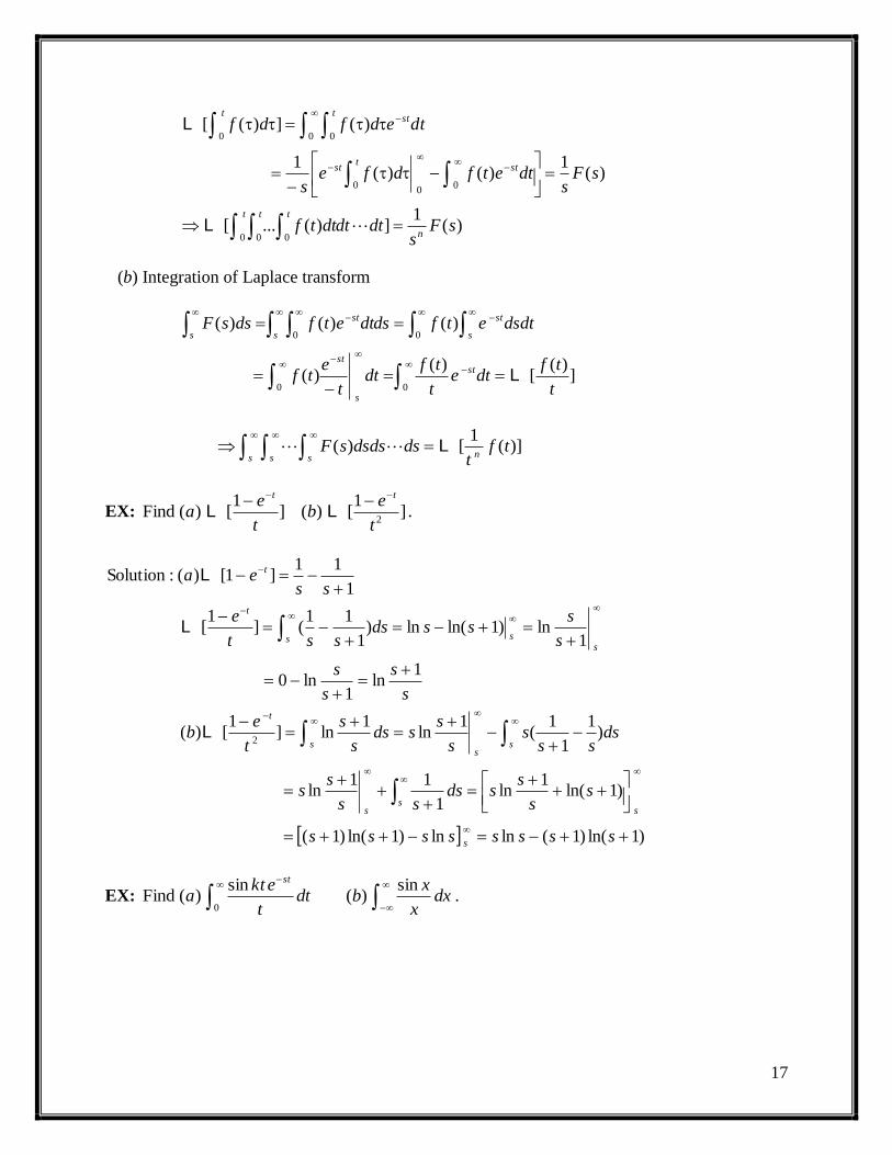
5. Integration
(a) Integral of original function
17
)(1
])(...[
)(1
)()(1
)(])([
0 0 0
00
0
0 00
sFs
dtdtdttf
sFs
dtetfdfes
tdedfdf
n
t t t
stt
st
tst
t
L
L
(b) Integration of Laplace transform
])(
[)(
)(
)()()(
00
0 0
t
tfdte
t
tfdt
t
etf
dsdtetfdtdsetfdssF
st
s
st
s s
stst
s
L
)](1
[)( tft
dsdsdssFns s s
L
EX: ]1
[)(]1
[)(Find2t
eb
t
ea
tt LL .
)1ln()1(lnln)1ln()1(
)1ln(1
ln1
11ln
)1
1
1(
1ln
1ln]
1[)(
1ln
1ln0
1ln)1ln(ln)
1
11(]
1[
1
11]1[)(:Solution
2
ssssssss
ss
ssds
ss
ss
dsss
ss
ssds
s
s
t
eb
s
s
s
s
s
sssds
sst
e
ssea
s
ss
s
s ss
t
sss
t
t
L
L
L
EX:
dxx
xbdt
t
ekta
st sin)(
sin)(Find
0.

18
)tan2
(lim2
sinlim2
sin2
sin)(
tan2
tan
1)(
11]
sin[
][sin
]sin
[sin
)(:Solution
1
01
001
0
11
222
22
0
k
s
dtt
kte
dxx
xdx
x
xb
k
s
k
s
ds
k
skds
ks
k
t
kt
ks
kkt
t
ktdt
t
ktea
sk
st
sk
s
s s
st
L
L
L
6. Convolution theorem
0 0
0 0 0
)(
00
0 0 0
)()()()(
)()(])()([
then,,Let
)()()()(
)()(])()([
sGsFdueugdef
dudeugfdtgf
dtdutu
dtdetgfdtdetgf
dtedtgfdtgf
sus
tus
stst
t tst
L
L t
t=
EX: .2sinoftransformLaplacetheFind0 t
t de
)4)(1(
2
4
2
1
1
]2[sin][]2sin*[]2sin[
4
2]2[sin,
1
1][:Solution
22
0
2
ssss
tetedte
st
se
ttt
t
t
LLLL
LL

19
7. Periodic Function: f (t + T) =f (t)
T
T
T TsusTTusst
T T
T
ststst
dueufedueTufdtetf
dtetfdtetfdtetftf
2
0 0
)(
0 0
2
)()()(and
)()()()]([ L
Similarly,
Tst
sT
TstsTsT
T
T
TsusTst
dtetfe
dtetfeetf
dueufedtetf
0
0
2
3
2 0
2
)(1
1
)()1()]([
)()(
L
EX: )()(,0,)(oftransformLaplacetheFind tfptfpttp
ktf .
)1
()1(
)1
()1(
)](1
[1
1
1
1)]([:Solution
0
00
0
ss
epe
eps
k
es
teeps
k
dtetesp
k
e
dttep
k
etf
spsp
ps
p
stst
ps
pst
pst
ps
pst
ps
L
8. Initial Value Theorem:
)(
)(lim
)(
)(lim:theoremvalueinitialgeneralDeduce
)(lim)(limtheoremvalueinitialgetwe
)0()(lim0)0()(lim)('lim)0()()]('[
0
0
0
sG
sF
tg
tf
ssFtf
fssFfssFdtetffssFtf
st
st
ss
st
s
L
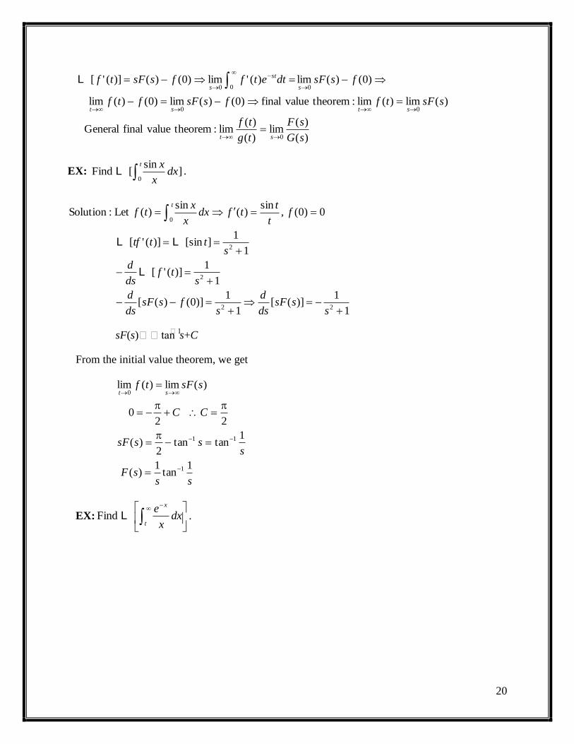
9. Final Value Theorem:
20
)(
)(lim
)(
)(lim:theoremvaluefinalGeneral
)(lim)(lim:theoremvaluefinal)0()(lim)0()(lim
)0()(lim)('lim)0()()]('[
0
00
000
sG
sF
tg
tf
ssFtffssFftf
fssFdtetffssFtf
st
stst
s
st
s
L
EX: ]sin
[Find0t
dxx
xL .
1
1)]([
1
1)]0()([
1
1)]('[
1
1][sin)]('[
0)0(,sin
)(sin
)(Let:Solution
22
2
2
0
sssF
ds
d
sfssF
ds
d
stf
ds
d
stttf
ft
ttfdx
x
xtf
t
L
LL
sF(s)tan1
s+C
From the initial value theorem, we get
sssF
ssssF
CC
ssFtfst
1tan
1)(
1tantan
2)(
220
)(lim)(lim
1
11
0
EX:
t
x
dxx
eLFind .

21
s
ssFCC
ssFtf
CsssF
sssF
ds
d
sfssF
ds
d
settf
tft
etfdx
x
etf
st
t
t
t
x
x
)1ln()(and,000
)(lim)(lim:theoremvaluefinaltheFrom
)1ln()(
1
1)]([
1
1)]0()([
1
1][)]('[
0)(lim,)()(Let:Solution
0
LL
Note:
t
t
x
dxx
edx
x
x
0and,
sinare called sine, and exponential integral function, respectively.
Module-II
INTERPOLATION AND INVERSE LAPLACE TRANSFORMS
INTERPOLATION
Introduction:-
If we consider the statement 0 ny f x x x x we understand that we can
find the value of y, corresponding to every value of x in the range 0 nx x x . If
the function f x is single valued and continuous and is known explicitly then the
values of f x for certain values of x like 0 1, ,......... nx x x can be calculated. The
problem now is if we are given the set of tabular values
0 1 2
0 1 2
: ........
: ........
n
n
x x x x x
y y y y y
Satisfying the relation y f x and the explicit definition of f x is not
known, then it is possible to find a simple function say f x such that f x and x
agree at the set of tabulated points. This process to finding x is called interpolation. If x

22
is a polynomial then the process is called polynomial interpolation and x is called
interpolating polynomial. In our study we are concerned with polynomial interpolation
Errors in Polynomial Interpolation:-
Suppose the function y x which is defined at the points
, 0,1,2,3i ix y i n is continuous and differentiable 1n times let n x be
polynomial of degree not exceeding n such that , 1,2 1n i ix y i n be the
approximation of y x using this n ix for other value of x, not defined by (1) the error is
to be determined
since 0 10 , ,......n ny x x for x x x x we put
1n ny x x L x
Where 1 0 ......... 3n nx x x x x and L to be determined such that the
equation (2) holds for any intermediate value of x such as 1 1
0, nx x x x x
Clearly
1 1
1
1
4n
n
y x xL
x
We construct a function F x such that 1
nF x F x F x . Then F x vanishes
2n times in the interval 0 , nx x . Then by repeated application of Rolle‟s theorem.
1F x must be zero 1n times, 11F x must be zero n times…….. in the interval 0 , nx x .
Also 1 0nF x once in this interval. suppose this point is x , 0 nx x
differentiate (5) 1n times with respect to x and putting x , we get
1 1 ! 0ny L n which implies that
1
1 !
nyL
n
Comparing (4) and (6) , we get
1
1 1 1
11 !
n
n n
yy x x x
n

23
Which can be written as
1 1
1 !
n n
n
xy x x y
n
This given the required expression 0 nx x for error
Finite Differences:-
1.Introduction:-
In this chapter, we introduce what are called the forward, backward and
central differences of a function y f x . These differences and three standard examples
of finite differences and play a fundamental role in the study of differential calculus, which
is an essential part of numerical applied mathematics
2.Forward Differences:-
Consider a function y f x of an independent variable x. let
0 1 2, , ,.... ry y y y be the values of y corresponding to the values 0 1 2, , .... rx x x x of x
respectively. Then the differences 1 0 2 1,y y y y are called the first forward
differences of y, and we denote them by 0 1, ,.......y y that is
0 1 0 1 2 1 2 3 2, , .........y y y y y y y y y
In general 1 0,1,2r r ry y y r
Here, the symbol is called the forward difference operator
The first forward differences of the first forward differences are called second forward
differences and are denoted by 2 2
0 1, ......y y that is
2
0 1 0
2
1 2 1
y y y
y y y
In general 2
1 0,1,2.......r r ry y y r similarly, the nth
forward differences are
defined by the formula.
1 1
1 0,1,2.......n n n
r r ry y y r
While using this formula for 1n , use the notation 0
r ry y and we have
0 1,2...... 0,2,.........n
ry n and r the symbol n is referred as the nth
forward
difference operator.
3. Forward Difference Table:-
The forward differences are usually arranged in tabular columns as shown in
the following table called a forward difference table
Values
of x
Values
of y
First
differences
Second
differences
Third
differences
Fourth
differences
ox 0y
0 1 0y y y

24
1x 1y 2
0 1 0y y y
1 2 1y y y 3 2 2
0 1 0y y y
2x 2y 2
1 2 1y y y
4 3 3
0 1 0y y y
2 3 2y y y 3 2 2
1 2 1y y y
3x 3y 2
2 3 2y y y
4y
34 yy
Example finite forward difference table for 3y x
x y f x y 2 y 3 y
4 y
1 1
7
2 8 12
19 6
3 27 18 0
37 6
4 64 24 0
61 6
5 125 30
91
6 216
4. Backward Differences:-
As mentioned earlier, let 0 1, ...... ......ry y y be the values of a function y f x
corresponding to the values 0 1 2, , ............. ......rx x x x of x respectively. Then,
1 1 0 2 2 1 3 3 2, , ,....y y y y y y y y y are called the first backward differences
In general 1, 1,2,3......... 1r r ry y y r
The symbol is called the backward difference operator, like the operator , this
operator is also a linear operator
25
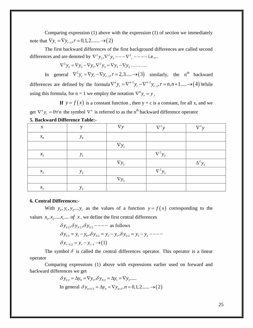
Comparing expression (1) above with the expression (1) of section we immediately
note that 1, 0,1,2....... 2r ry y r
The first backward differences of the first background differences are called second
differences and are denoted by 2 2 2
2 3, ry y i.e.,..
2 2
2 2 1 3 3 2,y y y y y y ……….
In general 2
1, 2,3..... 3r r ry y y r similarly, the nth
backward
differences are defined by the formula 1 1
1, , 1..... 4n n n
r r ry y y r n n
While
using this formula, for n = 1 we employ the notation 0
r ry y
If y f x is a constant function , then y = c is a constant, for all x, and we
get 0n
ry n the symbol n is referred to as the nth
backward difference operator
5. Backward Difference Table:-
x y y 2 y 3 y
0x 0y
1y
1x 1y 2
2y
6. Central Differences:-
With as the values of a function corresponding to the
values , we define the first central differences
as follows
The symbol is called the central differences operator. This operator is a linear
operator
Comparing expressions (1) above with expressions earlier used on forward and
backward differences we get
In general
2y 2
3y
2x 2y 2
3y
3y
3x 3y
0 1 2, , .... ry y y y y f x
1 2, ..... ....rx x x of x
1/2 3/2 5/2, ,y y y
1/2 1 0 3/2 2 1 5/2 3 2, ,y y y y y y y y y
1/2 1 1r r ry y y
1/2 0 1 3/2 1 2, .....y y y y y y
1/2 1, 0,1,2...... 2n n ny y y n

26
The first central differences of the first central differences are called the second
central differences and are denoted by
Thus
Higher order central differences are similarly defined. In general the nth
central
differences are given by
i) for odd
ii) for even
while employing for formula (4) for , we use the notation
If y is a constant function, that is if a constant, then
7. Central Difference Table
Example: Given from the central
difference table and write down the values of by taking
Sol. The central difference table is
-2 12
4
-1 16 -5
-1 9
0 15 4 -14
3 -5
1 18 -1
2 2
1 2, ...y y
2 2
1 3/2 1/2 2 5/2 3/2, .......y y y
2
1/2 1/2 3n n ny y y
1 1
1/2 1: , 1,2.... 4n n n
r r rn y y y r
1 1
1/2 1/2: , 1,2.... 5n n n
r r rn y y y r
1n 0
r ry y
y c
0 1n
ry for all n
2 12, 1 16, 0 15, 1 18, 2 20f f f f f
2 3
3/2 0 7/2,y y and y 0 0x
x y f x y 2 y 3 y 4 y
0x 0y y 2 y 3 y 4 y
1/2y
1x 1y 2
1y
2/2y 3
3/2y
2x 2y 2
2y 4
2y
5/2y 3
5/2y
3x 3y 2
3y
7/2y
4x 4y

27
2
2 20
Symbolic Relations and Separation of symbols:
We will define more operators and symbols in addition to , and already
defined and establish difference formulae by symbolic methods
Definition:- The averaging operator is defined by the equation
Definition:- The shift operator E is defined by the equation . This shows that the
effect of E is to shift the functional value to the next higher value . A second
operation with E gives
Generalizing
Relationship Between
We have
Some more relations
Definition
Inverse operator is defined as
In general
We can easily establish the following relations
i)
ii)
iii)
iv)
v)
Definition The operator D is defined as
Relation Between The Operators D And E
1/2 1/2
1
2r r ry y y
1r rEy y
ry 1ry
2
1 2r r r rE y E Ey E y y
n r
r nE y y
and E
33 3 2
0 0 0
3 2 1 0
1 3 3 1
3 3
y E y E E E y
y y y y
1E 1
1r rE y y
n
n r nE y y
11 E 1/2 1/2E E
1/2 1/21
2E E
1/2E E
2 211
4
Dy x y xx
0 1 0
0 0 01
1
y y y
Ey y E y
E y or E

28
Using Taylor’s series we have,
This can be written in symbolic form
We obtain in the relation
If is a polynomial of degree n and the values of x are equally spaced then
is constant
Proof:
Let where are constants and
. If h is the step- length, we know the formula for the first forward difference
Where are constants. Here this polynomial is of degree , thus,
the first difference of a polynomial of nth
degree is a polynomial of degree
Now
Where are constants. This polynomial is of degree
Thus, the second difference of a polynomial of degree n is a polynomial of degree
continuing like this we get
2 3
1 11 111
2! 3!
h hy x h y x hy x y x y x
2 2 3 3
1 .2! 3! X
hD
x x
h D h DEy hD y e y
3hDE e
f x
n f x
1
0 1 1
n n
n nf x a x a x a x a
0 1 2, , .... na a a a
0 0a
1
0 1 1
1
0 1 1
n n
n n
n n
n n
f x f x h f x a x h a x h a x h a
a x a x a x a
1 2 2
0
1 2 3 2 1
1
1
1 2 3
0 2 3 3 2
1. .
2!
1 21 . .
2!
n n n n
n n n n
n
n n n
n n
n na x n x h x h x
n na x n x h x h x
a h
a nhx b x b x b x b
2 3 2, ,....... nb b b 1n
1n
2
1 2 3
0 2 3 1 2
1 21 2
0 2 1
1 2 2 3
0 3 4 3
. n n n
n n
n nn n
n
n n n
n n
f x f x
a nh x b x b x b x b
a nh x h x b x h x b x h x
a n h x c x c x c
3 3.... nc c 2n
2n
0 01 2 2.1. !n n nf x a n n n h a h n
29
which is constant
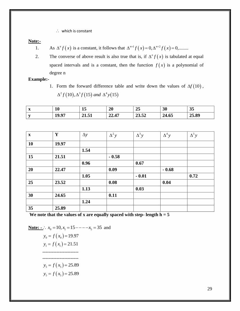
Note:-
1. As is a constant, it follows that
2. The converse of above result is also true that is, if is tabulated at equal
spaced intervals and is a constant, then the function is a polynomial of
degree n
Example:-
1. Form the forward difference table and write down the values of ,
x 10 15 20 25 30 35
y 19.97 21.51 22.47 23.52 24.65 25.89
x Y
10 19.97
1.54
15 21.51 - 0.58
0.96 0.67
20 22.47 0.09 - 0.68
1.05 - 0.01 0.72
25 23.52 0.08 0.04
1.13 0.03
30 24.65 0.11
1.24
35 25.89
We note that the values of x are equally spaced with step- length h = 5
Note: - and
-----------------------
-----------------------
n f x 1 20, 0,........n nf x f x
n f x
f x
10f
2 3 410 , 15 15f f and y
y 2 y 3 y 4 y 5 y
0 1 510, 15 35x x x
0 0
1 1
19.97
21.51
y f x
y f x
5 5 25.89y f x
5 5 25.89y f x

30
From table
2. Evaluate
Sol. Let h be the interval of differencing
Proceeding on, we get
3. Using the method of separation of symbols show that
Sol. To prove this result, we start with the right hand side. Thus
0
2 2
0
3 3
1
4 3
1
10 1.54
10 0.58
15 0.01
15 0.04
f y
f y
f y
f y
2
cos
sin
n ax b
i x
ii px q
iii e
cos cos cos
h2sin sin
2 2
sin sin sin
2cos sin2 2
2sin sin2 2 2
i x x h x
hx
ii px q p x h q px q
ph phpx q
ph phpx q
2 1sin 2sin sin
2 2
phpx q px q ph
2
12sin sin
2 2
phpx q ph
1
2
2
2
1
1
1
a x h bax b ax b
ax b ah
ax b ax b ah ax b
ah ax h
ah ax b
iii e e e
e e
e e e e
e e
e e
1n
n ax b ah ax be e e
1 2
11
2
nn
x n x n x x x n
n nn

31
which is left hand side
4. Find the missing term in the following data
x 0 1 2 3 4
y 1 3 9 - 81
Why this value is not equal to . Explain
Sol. Consider
Substitute given values we get
From the given data we can conclude that the given function is . To find ,
we have to assume that y is a polynomial function, which is not so. Thus we are not
getting Newton’s Forward Interpolation Formula:-
Let be a polynomial of degree n and taken in the following form
This polynomial passes through all the points for i = 0 to n. there
fore, we can obtain the by substituting the corresponding as
Let „h‟ be the length of interval such that represent
1 2
1 2 1
11 2 1
2
11
2
11 1 1
2
111
n
n n
nn n
nn
nn n
n
n nx n x x x n
n nx nE x E x E x
n nnE E E x E x
En n
E E
x E xE
n
x n
334
0 0y
0 3 2 1 04 4 5 4 0y y y y y
3 381 4 54 12 1 0 31y y
3xy 3y
33 27y
y f x
0 1 0 2 0 1 3 0 1 2
0 1 1 1n n
y f x b b x x b x x x x b x x x x x x
b x x x x x x
;xi yi
'iy s 'ix s
0 0 0
1 1 0 1 1 0
2 2 0 1 2 0 2 2 0 2 1
,
,
, 1
at x x y b
at x x y b b x x
at x x y b b x x b x x x x
'ix s
0 0 0 0 0, , 2 , 3x x h x h x h x xh

32
This implies
From (1) and (2), we get
Solving the above equations for , we get
Similarly, we can see that
If we use the relationship
Then
1 0 2 0 3 0 0, 2 , 3 2nx x h x x h x x h x x nh
0 0
1 0 1
2 0 1 2
3 0 1 2 3
0 1 2
2 2
3 3 2 3 2
.....................................
.....................................
1 1 2 3n n
y b
y b b h
y b b h b h h
y b b h b h h b h h h
y b b nh b nh n h b nh n h n h
0 11 2, , ..... nb b b b 0 0b y
1 0 1 0 01
1 02 0 12 2 02
22
2
y b y y yb
h h h
y yy b b hb y y h
h h
2
2 0 1 0 2 1 0 0
2 2 2
2
02 2
2 2 2
2 2 2
2!
y y y y y y y y
h h h
yb
h
3 4
0 0 03 43 4
2
0 00 0 0 12
,3! 4! !
2!
n
n n
y y yb b b
h h n h
y yy f x y x x x x x x
h h
3
00 1 23
00 1 1
3!
3!
n
nn
yx x x x x x
h
yx x x x x x
n h
0 0 , 0,1,2,.....x x ph x x ph where p n

33
Equation (3) becomes
Newton’s Backward Interpolation Formula:-
If we consider
and impose the condition that y and should agree at the tabulated points
We obtain
Where
This uses tabular values of the left of . Thus this formula is useful formula is useful
for interpolation near the end of the table values
Formula for Error in Polynomial Interpolation:-
If is the exact curve and is the interpolating curve, then
the error
in polynomial interpolation is given by
for any x, where
1 0 0
2 1 1
1
1
1 2
............................................
............................................
1
i
n
x x x x h x x h
ph h p h
x x x x h x x h
p h h p h
x x p i h
x x p n h
2 3
0 0 0 0 0
0
1 1 2
2! 3!
1 2 14
!
n
p p p p py f x f x ph y p y y y
p p p p ny
n
0 1 2 1 3 1 2n n n n n n n iy x a a x x a x x x x a x x x x x x x x
ny x
2 1 0, 1,...... , ,n nx x x x x
21
2
1 16
!
n n n n
n
n
p py x y p y y
i
p p p ny
n
nx xp
h
ny
y f x ny x
0 1 1 7
1 !
n n
n
x x x x x xError f x x f
n
0 0n nx x x and x x

34
The error in Newton‟s forward interpolation formula is given by
Where
The error in Newton‟s backward interpolation formula is given by
Where
Examples:-
1. Find the melting point of the alloy containing 54% of lead, using appropriate
interpolation formula
Percentage of
lead(p) 50 60 70 80
Temperature 205 225 248 274
Sol. The difference table is
x Y
50 205
20
60 225 3
23 0
70 248 3
26
80 274
Let temperature =
By Newton‟s forward interpolation formula
Melting point = 212.64
1
1 2 .......
1 !
n
n
p p p p nf x x f
n
0x xp
h
1 1
1 2 .......
1 !
n n
n
p p p p nf x x h y f
n
nx xp
h
Q c
2 3
f x
0 024, 50, 10
50 10 54 0.4
x ph x h
p or p
2 3
0 0 0 0 0
1 1 2
2! !
0.4 0.4 1 0.4 0.4 1 0.4 254 205 0.4 20 3 0
2! 3!
205 8 0.36
212.64
p p p p pf x ph y p y y y
n
f

35
2. Using Newton‟s forward interpolation formula, and the given table of values
X 1.1 1.3 1.5 1.7 1.9
0.21 0.69 1.25 1.89 2.61
Obtain the value of
Sol.
x
1.1 0.21
0.48
1.3 0.69 0.08
0.56 0
1.5 1.25 0.08 0
0.64 0
1.7 1.89 0.08
0.72
1.9 2.61
If we take ,
Using Newton’s interpolation formula
f x
1.4f x when x
y f x 2 3 4
0 01.3 0.69x then y
2 3
0 0 0
0
0.56, 0.08, 0, 0.2, 1.3
11.4 1.3 0.2 1.4,
2
y y y L x
x ph or p p
1 11
1 2 21.4 0.69 0.56 0.08
2 2!
0.69 0.28 0.01 0.96
f
36
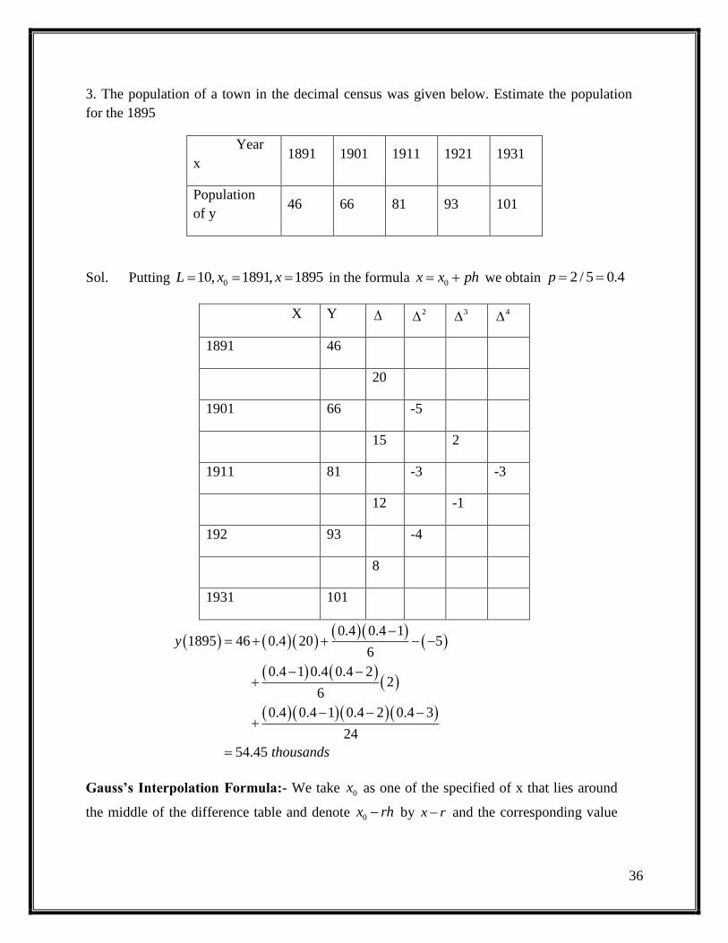
3. The population of a town in the decimal census was given below. Estimate the population
for the 1895
Year
x 1891 1901 1911 1921 1931
Population
of y 46 66 81 93 101
Sol. Putting in the formula we obtain
X Y
1891 46
20
1901 66 -5
15 2
1911 81 -3 -3
12 -1
192 93 -4
8
1931 101
Gauss’s Interpolation Formula:- We take as one of the specified of x that lies around
the middle of the difference table and denote by and the corresponding value
010, 1891, 1895L x x 0x x ph 2 / 5 0.4p
2 3 4
0.4 0.4 11895 46 0.4 20 5
6
0.4 1 0.4 0.4 22
6
0.4 0.4 1 0.4 2 0.4 3
24
54.45
y
thousands
0x
0x rh x r

37
of y by . Then the middle part of the forward difference table will appear as shown in
the next page
X Y
By using the expressions (1) and (2), we now obtain two versions of the following Newton‟s
forward interpolation formula
y r
y 2 y 3 y 4 y 5 y
4x 4y
3x 3y 4y
2x 2y 3y 2
4y
1x 1y 2y 2
3y 3
4y
0x 0y 1y 2
2y 3
3y 4
4y
1x 1y 0y 2
1y 3
2y 4
3y 5
4y
2x 2y 1y 2
0y 3
1y 4
2y 5
3y
3x 3y 2y 2
1y 3
0y 4
1y 5
2y
4x 4y 3y 2
2y 3
1y 4
0y 5
1y
2
0 1 1
2 2 3
0 1 1
3 3 4
0 1 1
4 4 5
0 1 1
2
1 2 2
2 2 3
1 2 2
3 3 4
1 2 2
4 4 5
1 2 2
1
2
y y y
y y y
y y y
y y y and
y y y
y y y
y y y
y y y
2 3
0 0 0 0
4
0
1 1 2[
2! 3!
1 2 3] 3
4!
p
p p p p py y p y y y
p p p py
-----------------3
38
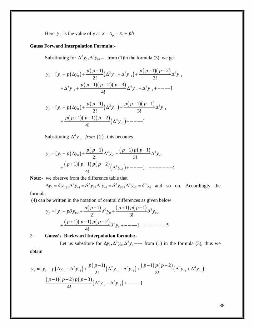
Here is the value of y at
Gauss Forward Interpolation Formula:-
Substituting for from (1)in the formula (3), we get
Substituting , this becomes
Note:- we observe from the difference table that
and so on. Accordingly the
formula
(4) can be written in the notation of central differences as given below
2. Gauss’s Backward Interpolation formula:-
Let us substitute for ----- from (1) in the formula (3), thus we
obtain
py 0px x x ph
2 3
0 0, ,....y y
2 3 3
0 0 1 1 1
4 4 5
1 1 1
1 1 2[
2! 3!
1 2 3]
4!
p
p p p p py y p y y y y
p p p py y y
2 3
0 0 1 1
4
1
1 1 1[
2! 3!
1 1 2]
4!
p
p p p p py y p y y y
p p p py
4
1 2y from
2 3
0 0 1 1
4
2
1 1 1[
2! 3!
1 1 2] 4
4!
p
p p p p py y p y y y
p p p py
2 2 3 3 4 4
0 1/2 1 0 1 1/2 2 0, , ,y y y y y y y y
2 3
0 1/2 0 1/2
4
0
1 1 1[
2! 3!
1 1 2] 5
4!
p
p p p p py y p y y y
p p p py
2 3
0 0 0, ,y y y
2 2 3 3 4
0 1 1 1 1 1 1
4 5
1 1
1 1 2[
2! 3!
1 2 3]
4!
p
p p p p py y p y y y y y y
p p p py y
-----------------5
-----------------4

39
Substituting for and from (2) this becomes
Lagrange’s Interpolation Formula:-
Let be the values of x which are not necessarily
equally spaced. Let be the corresponding values of let the
polynomial of degree n for the function passing through the points
be in the following form
Where an are constants
Since the polynomial passes through , .
The constants can be determined by substituting one of the values of
in the above equation
Putting in (1) we get,
Putting in (1) we get,
Similarly substituting in (1), we get
Continuing in this manner and putting in (1) we
get
Substituting the values of , we get
2 3 4
0 1 1 1 1
1 1 1 1 1 2[ ]
2! 3! 4!
p p p p p p p py p y p y y y
3
1y 4
1y
2 3 4
0 1 1 1 2
4 5
2 2
1 1 1[
2! 3!
1 1 2]
4!
p
p p p p py y p y y y y
p p p py y
0 1 2, , ,....x x x nx 1n
0 1 2, , ........ ny y y y y f x
y f x 1n
0 0 1 1, , , ,n nx f x x f x x f x
0 1 2 1 0 2
2 0 1 0 1 1
...... .........
....... ........ ...... 1
n n
n n n
y f x a x x x x x x a x x x x x x
a x x x x x x a x x x x x x
0 1 2, , ....a a a
0 0,x f x 1 1, ...... ,n nx f x x f x
0 1, ,..... nx x x for x
0x x 0 0 1 0 2 0 nf x a x x x x x x
0
0
1 0 2 0.... n
f xa
x x x x x x
1x x 1 1 0 1 2 1 nf x a x x x x x x
1
1
1 0 1 2 1.... n
f xa
x x x x x x
2x x
2
2
2 0 2 1 2...... n
f xa
x x x x x x
nx x
0 1 1
n
n
n n n n
f xa
x x x x x x
0 1 2, , .... na a a a

40
Examples:-
1. Using Lagrange‟s formula calculate from the following table
x 0 1 2 4 5 6
1 14 15 5 6 19
Sol. Given
From langrange‟s interpolation formula
Here then
1 2 0 2
0
0 1 0 2 0 1 0 1 2 1
....... .....
......... ....
n n
n n
x x x x x x x x x x x xf x f x
x x x x x x x x x x x x
0 1 2 0 1 1
1 2
2 0 2 1 2 1 2 1
..... ..........
...... .....
n n
n
n n n n n
x x x x x x x x x x x x x xf x f x f x
x x x x x x x x x x x x
3f
f x
0 1 2 3 5 40, 1, 2, 4, 6, 5x x x x x x
0 1 2 3 4 51, 14, 15, 5, 6, 19f x f x f x f x f x f x
1 2 3 4 5
0
0 1 0 2 0 3 0 4 0 5
0 2 3 4 5
1
1 0 1 2 1 3 1 4 1 5
0 1 3 4 5
2
2 0 2 1 2 3 2 4 2 5
0 1
x x x x x x x x x xf x f x
x x x x x x x x x x
x x x x x x x x x xf x
x x x x x x x x x x
x x x x x x x x x xf x
x x x x x x x x x x
x x x x x x
2 3 4
5
5 0 5 1 5 2 5 3 5 4
x x x xf x
x x x x x x x x x x
3x
3 1 3 2 3 4 3 5 3 63 1
0 1 0 2 0 4 0 5 0 6
3 0 3 2 3 4 3 5 3 614
1 0 1 2 1 4 1 5 1 6
3 0 3 1 3 4 3 5 3 615
2 0 2 1 2 4 2 5 2 6
f

41
1) Find using lagrange method of and order degree polynomials.
Sol: By lagrange‟s interpolation formula
For ,we have
3 0 3 1 3 2 3 5 3 65
4 0 4 1 4 2 4 5 4 6
3 0 3 1 3 2 3 4 3 66
5 0 5 1 5 2 5 4 5 6
3 0 3 1 3 2 3 4 3 519
6 0 6 1 6 2 6 4 6 5
12 18 36 36 18 1214 15 5 6 19
240 60 48 48 60 40
0.05 4.2 11.25 3.75 1.8 0.95
10
3 10f x
3.5f 2nd 3rd
x 1 2 3 4
1 2 9 28f x
0 1 1
0 0 1
.......
....... .......
nk k n
k
k k k k k n
x x x x x x x xf x f x
x x x x x x
4n
1 2 3
0
0 1 0 2 0 3
x x x x x xf x f x
x x x x x x
0 2 3
1
1 0 1 2 1 3
0 1 3
2
2 0 2 1 2 3
0 1 2
3
3 0 3 1 3 2
x x x x x xf x
x x x x x x
x x x x x xf x
x x x x x x
x x x x x xf x
x x x x x x
3.5 2 3.5 3 3.5 43.5 1
1 2 1 3 1 4f
3.5 1 3.5 3 3.5 42
2 1 2 3 2 4

42
- - - -
=0.0625+(-0.625)+8.4375+8.75
=16.625
Example:
Find y(25), given that y20 = 24,y24 = 32, y28 = 35 y32 = 40 using Guass forward
difference Formula :
Solution: Given
x 20 24 28 32
y 24 32 35 40
By Gauss Forward difference formula
We take x= 24 as origin.
X0 = 24, h = 4, x = 25 p = x-x0/ h, p = 25-24/4 = 2.5
3.5 1 3.5 2 3.5 49
3 1 3 2 3 4
3.5 1 3.5 2 3.5 328
4 1 4 2 4 3
2 3 4 1 3 41 2
6 2
1 2 4 1 2 39 28
2 6
x x x x x xf x
x x x x x x
2 2 2
25 6 4 3 2 3 2
4 3 4 4 9 3 286 2 6
x x x x x x xx x x x x
3 2 3 2 3 2
3 29 26 24 7 14 8 6 11 68 9 12 9 28
6 2 6
x x x x x x x x xx x x
3 2 3 2 3 2 3 29 26 24 6 48 114 72 27 189 378 216 308 28 168 168
6
x x x x x x x x x x x x
3 2
3 26 18 183 3
6
x x xf x x x x
3 2
3.5 3.5 3 3.5 3 3.5 16.625f
2 3 3
0 0 1 1 1
4 4 5
1 1 1
1 1 2[
2! 3!
1 2 3]
4!
p
p p p p py y p y y y y
p p p py y y

43
Gauss Forward difference table is
X y
20
24
24
32
= 8
28
35
= 3 = -
5
32 40
= 5 = 2 = 7
By gauss Forward interpolation Formula
We y(25) = 32 +.25(3) + (.25)(.25−1)
2(−5) +
.25+1 .25 .25−1
6 7 = 32 + .75
+ .46875 - .2734 = 32.945
Y(25) = 32.945.
Example:
Use Gauss Backward interpolation formula to find f(32) given that f(25) = .2707, f(30)
= .3027, f(35) = .3386 f(40) = .3794.
Solution: let x0 = 35 and difference table is
X y
25
.2707
30
.3027
.032
35
.3386 .0359
.0039
40 .3794
.0408
.0049
.0010
From the table y0 = 0.3386
= 0.0359 , = 0.0049, = 0.0010, xp = 32 p = xp- x0/h = 32-35/5 = -.6
By Gauss Backward difference formula
f(32) = .3386 + (-.6)(.0359) + (-.6)(-.6+1)(.0049)/2 + (-.6)(.36-1)(0.00010)/6 = .3165
INVERSE LAPLACE TRANSFORMS
I. Inversion from Basic Properties
1. Linearity
Ex. 1.
]16
)1(4[)(]
4
12[)(
2
1
2
1
s
sb
s
sa LL .
y 2 y 3 y
1y
0y 2
1y
1y 2
0y 3
1y
y 2 y 3 y
1y2
1y 3
2y

44
ttss
s
s
sb
ttss
s
s
sa
4sinh4cosh4]4
4
44[]
16
)1(4[)(
2sin2
12cos2]
2
2
2
1
22[]
4
12[)(:Solution
2222
1
2
1
2222
1
2
1
LL
LL
2. Shifting
Ex. 2.
]23
32[)(]
22[)(
2
1
2
1
ss
sb
ss
ea
s
LL .
2cosh2]
)2
1()
2
3(
)2
3(2
[]23
32[)(
)(sin)()sin(]1)1(
[
)()]()([and
sin]1)1(
1[
]1)1(
[]22
[)(:Solution
2
3
22
1
2
1
)()(
2
1
2
1
2
1
2
1
te
s
s
ss
sb
ttuetutes
e
sFeatuatf
tes
s
e
ss
ea
t
tts
as
t
ss
LL
L
L
L
LL
3. Scaling
Ex. 3.
]416
4[
2
1
s
sL .
2cosh
4
1
4
12cosh
4
1]
2)4(
4[]
416
4[:Solution
22
1
2
1 tt
s
s
s
s
LL
4. Derivative
Ex. 4.
][ln)(])(
1[)( 1
222
1
bs
asb
sa
LL .

45
)cos(sin2
1)]('sin2[
2
1]
)(
1[
)]('sin2[2
1
)(
1
)(
2][sin2
])(
1[2]
)(
)([2
)(2)]('[
)0()(
2)]('[sin)(Let
)(
2)(]sin[][sin)(:solution
33222
1
3222
222
3
222
2
22222
222
222
2
222
2222222
ttttFts
tFts
st
sss
s
s
stF
Fs
sstFtttF
s
s
sds
dtt
sta
L
L
L
L
L
LL
t
eetf
eeasbs
bsasds
dttf
bsasbs
astfb
atbt
atbt
)(
][11
)]ln()[ln()]([
)ln()ln(ln)]([Let)(
LL
L
5. Integration
Ex. 5.
][ln)()]1
1(
1[)( 1
2
1
bs
asb
s
s
sa
LL .
t
ee
bs
as
bs
as
as
bsds
asbst
ee
asbseeb
teteedtee
dtdtedtesssss
s
sa
atbt
ss
atbt
atbt
tt
tttt
t t ttt
][ln
lnln)11
(][
11][)(
22)1()1()1()1(
])1(
1
)1(
1[)]
1
1(
1[)(:Solution
1
0
0 0 02
1
2
1
L
L
L
LL
6. Convolution
Ex. 6.
])(
[)(])(
1[)(
222
1
222
1
s
sb
sa LL .

46
)cos(sin2
1}cos)]sin((sin
2
1{[
2
1
cos)2sin(2
1
2
1]cos)2[cos(
2
1
)]cos()[cos(2
11
)(sinsin1
])(
1[
1]sin
1[][sin)(:Solution
32
0
202
02
02222
1
2222
ttttttt
ttdtt
dtt
dts
st
sta
tt
t
t
L
LL
tt
tttt
ttdtt
dtt
dts
s
s
st
stb
tt
t
t
sin2
)]}cos([cos2
1sin{
2
1
)2cos(2
1sin
2
1)]2sin([sin
2
1
)]sin()[sin(2
11
)(cossin1
])(
[
][cos1
]sin1
[)(
00
0
0222
1
2222
L
LL
II. Partial Fraction
If F(s))(
)(
sQ
sP, where deg[P(s)]<deg[Q(s)]
1.Q(s)0 with unrepeated factors sai
ta
n
ntata
n
nn
k
k
ask
k
aSkk
aSk
n
n
n
k
kk
eaQ
aPe
aQ
aPe
aQ
aP
sQ
sP
as
aQaP
as
aQaP
as
aQaP
sQ
sP
aQ
aP
sQaP
sQ
asaPas
sQ
sPA
as
A
as
A
as
A
sQ
sP
)('
)(
)('
)(
)('
)(]
)(
)([
)('/)()('/)()('/)(
)(
)(
)('
)(
)('
1lim)(
)(lim)()](
)(
)([lim
)(
)(
21
2
2
1
11
2
22
1
11
2
2
1
1
L

47
Ex. 7.
]6
1[
23
1
sss
s
L .
tt
s
s
s
eessssss
s
ss
sA
ss
sA
ss
sA
s
A
s
A
s
A
sss
s
sss
s
32
23
1
33
22
01
321
23
15
2
10
3
6
1
3
15
2
2
10
3
6
1
]6
1[
15
2
)2(
1lim
10
3
)3(
1lim
6
1
)3)(2(
1lim
32)3)(2(
1
6
1:Solution
L
2. Q(s)0 with repeated factors (sak)m
])!2()!1(
[])(
)([
)!1(
1]})(
)(
)([{lim
!2
1]})(
)(
)([{lim
]})()(
)([{lim
])()(
)([lim
)()()()()(
)(
)()()(
)(
122
1
11
1
1
1
2
2
2
1
1
1
2
21
1
1
1
CtCm
tC
m
tCe
sQ
sP
mas
sQ
sP
ds
dC
assQ
sP
ds
dC
assQ
sP
ds
dC
assQ
sPC
asCasCasCCassQ
sP
as
C
as
C
as
C
sQ
sP
mm
m
m
ta
m
km
m
as
m
kas
m
m
kas
m
m
kas
m
m
kkmkmm
m
k
k
m
k
m
m
k
m
k
k
k
k
k
L
Ex. 8.
])3)(2)(1(
124137[
2
2341
ssss
ssssL .

48
ttt
s
s
s
s
s
eeetssss
ssss
sss
ssssA
sss
ssssA
sss
ssssA
sss
ssss
ds
dC
sss
ssssC
s
A
s
A
s
A
s
C
s
C
ssss
ssss
32
2
2341
2
234
33
2
234
22
2
234
11
22
234
01
234
02
3211
2
2
2
234
2
12
2
132]
)3)(2)(1(
124137[
2
1
18
9
)2)(1(
124137lim
24
8
)3)(1(
124137lim
2
1
)3)(2(
124137lim
36
111224
)]3)(2)(1[(
)]2)(1()3)(1()3)(2)[(12()3)(2)(1(4
])3)(2)(1(
124137[lim
26
12
)3)(2)(1(
124137lim
321)3)(2)(1(
124137:Solution
L
3. Q(s)0 with unrepeated factor (s)2+, where >0
tBA
tAes
BAsA
sQ
sP
BAIA
RBA
ssQ
sPIR
iAAiIR
BiAssQ
sP
BAsssQ
sP
s
BAs
sQ
sP
t
is
is
sincos])(
)()([]
)(
)([
and,andgetcanwewhere,then,
lyrespective]},)[()(
)({limofpartsimaginaryandrealtheareandwhere
)(
)(]})[()(
)({lim
])[()(
)(
)()(
)(
22
11
22
22
22
22
LL
Ex. 9.
]4
[4
21
s
sL .
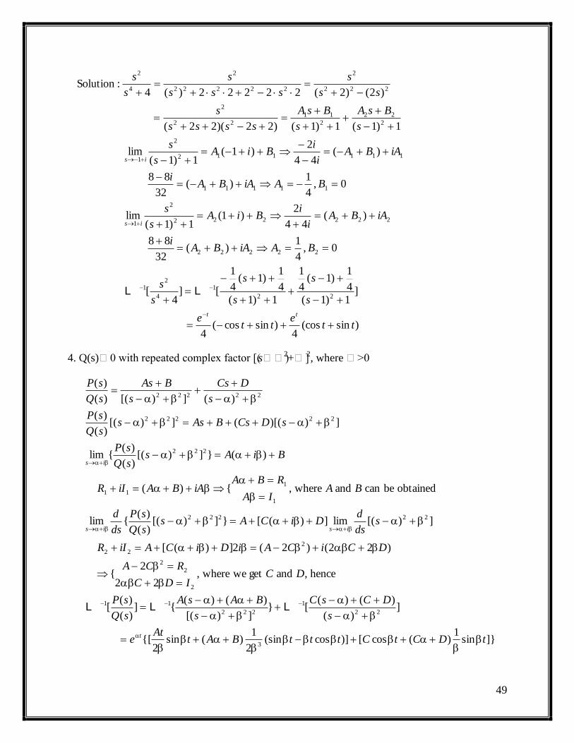
49
)sin(cos4
)sincos(4
]1)1(
4
1)1(
4
1
1)1(
4
1)1(
4
1
[]4
[
0,4
1)(
32
88
)(44
2)1(
1)1(lim
0,4
1)(
32
88
)(44
2)1(
1)1(lim
1)1(1)1()22)(22(
)2()2(22222)(4:Solution
22
1
4
21
22222
222222
2
1
11111
111112
2
1
2
22
2
11
22
2
222
2
22222
2
4
2
tte
tte
s
s
s
s
s
s
BAiABAi
iABAi
iBiA
s
s
BAiABAi
iABAi
iBiA
s
s
s
BsA
s
BsA
ssss
s
ss
s
sss
s
s
s
tt
is
is
LL
4. Q(s)0 with repeated complex factor [(s)2+]
2, where >0
]}sin1
)(cos[)]cos(sin2
1)(sin
2{[
])(
)()([}
])[(
)()({]
)(
)([
hence,andgetwewhere,22
2{
)22()2(2])([
])[(lim])([}])[()(
)({lim
obtainedbecanandwhere,{)(
)(}])[()(
)({lim
]))[((])[()(
)(
)(])[()(
)(
3
22
1
222
11
2
2
2
2
22
22222
1
1
11
222
22222
22222
tDCtCtttBAtAt
e
s
DCsC
s
BAsA
sQ
sP
DCIDC
RCA
DCiCAiDiCAiIR
sds
dDiCAs
sQ
sP
ds
d
BAIA
RBAiABAiIR
BiAssQ
sP
sDCsBAsssQ
sP
s
DCs
s
BAs
sQ
sP
t
isis
is
LLL

50
Ex. 10.
])22(
463[
22
231
ss
sssL .
)cossin()cossin2
2(
]1)1(
1[}
]1)1[(
)1(2{]
)22(
463[
1,1
)(2)2(2)(0
]1)1[(lim])1([)463(lim
2,2)(2
)1()463(lim
1)1(]1)1[()22(
463:Solution
2
1
22
1
22
231
2
1
23
1
23
1
22222
23
tttettt
e
s
s
s
s
ss
sss
Dc
DcicAiDiccA
sds
dDicAsss
ds
d
BAiABAi
BiAsss
s
Dcs
s
BAs
ss
sss
tt
isis
is
LLL
IV. Differentiation with Respect to a Number
Ex. 11.
])(
1[
222
1
sL .
)cos(sin2
1]
)(
1[
cossin1
)sin1
(]1
[])(
1[2
])(
2[)]
1([
)(
2)
1(:Solution
3222
1
222
1
222
1
222
1
22
1
22222
ttts
tt
ttd
d
sd
d
s
ssd
d
ssd
d
L
LL
LL
V. Method of Differential Equation
Ex. 12.
][1 seL .

51
t
s
s
t
t
s
t
s
t
t
ssss
et
y
c
s
s
e
t
ect
s
eect
s
eyty
ecttys
s
t
ectyct
ty
dtt
t
y
dyytytytyyt
dt
d
ytyytdt
dyyys
s
e
s
ey
s
eyey
4
1
2/3
02
1
4
1
2
1
4
1
2
1
4
1
2
1
2
12
1
4
1
2
3
1
2
22
2
3
2
1
2
12limlimtheoremvaluefinalgeneralApply
2][
2][while
][][and,
)2
1(
][
4
1ln
2
3ln
04
160)16('402)(4
0][][2)]([4024equationthegetwe
44,
2:Solution
LL
LLL
LLL
Applied to Solve Differential Equations
I. Ordinary Differential Equations with Constant Coefficients
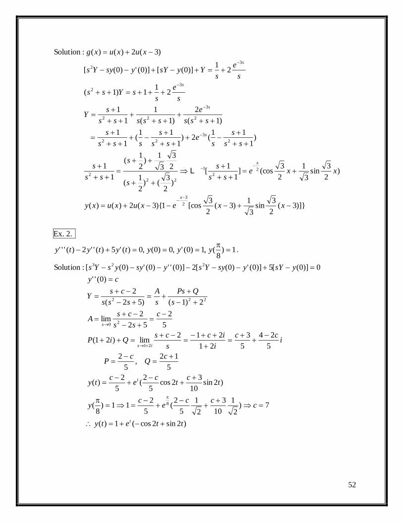
Ex. 1.
33
301)(where,0)0(',1)0(),('''
x
xxgyyxgyyy .
52
)]}3(2
3sin
3
1)3(
2
3[cos1){3(2)()(
)2
3sin
3
1
2
3(cos]
1
1[
)2
3()
2
1(
2
3
3
1)
2
1(
1
1
)1
11(2)
1
11(
1
1
)1(
2
)1(
1
1
1
21
1)1(
21
)]0([)]0(')0([
)3(2)()(:Solution
2
3
22
1
22
2
2
3
22
2
3
22
32
32
xxexuxuxy
xxess
s
s
s
ss
s
ss
s
se
ss
s
sss
s
sss
e
sssss
sY
s
e
ssYss
s
e
sYysYysyYs
xuxuxg
x
x
s
s
s
s
L
Ex. 2.
1)8
(,1)0(',0)0(,0)('5)(''2)('''
yyytytyty .
)2sin2cos(1)(
7)2
1
10
3
2
1
5
2(
5
211)
8(
)2sin10
32cos
5
2(
5
2)(
5
12,
5
2
5
24
5
3
21
212lim)21(
5
2
52
2lim
2)1()52(
2
)0(''
0)]0([5)]0(')0([2)]0('')0(')0([:Solution
8
21
20
222
223
ttety
ccc
ec
y
tc
tc
ec
ty
cQ
cP
icc
i
ic
s
csQiP
c
ss
csA
s
QPs
s
A
sss
csY
cy
ysYysyYsysyysYs
t
t
is
s

53
Module-III
CURVE FITTING AND FOURIER TRANSFORMS
Suppose that a data is given in two variables x & y the problem of finding an analytical
expression of the form which fits the given data is called curve fitting
Let be the observed set of values in an experiment and
be the given relation are the error of approximations
then we have
where are called the expected values of
y corresponding to
are called the observed values of y corresponding to
the differences between expected values of y and
observed values of y are called the errors, of all curves approximating a given set of points,
the curve for which
is a minimum is called the best fitting curve (or) the least
square curve
This is called the method of least squares (or) principles of least squares
1. FITTING OF A STRAIGHT LINE:-
Let the straight line be
Let the straight line (1) passes through the data points
So we have
The error between the observed values and expected values of is defined
as
The sum of squares of these error is
now for E to be minimum
These equations will give normal equations
y f x
1 1 2 2, , , ........ ,n nx y x y x y
y f x 1 2& , , ,...... xx y Let E E E
1 1 1
2 2 2
3 3 3
E y f x
E y f x
E y f x
n n nE y f x 1 2, ........... nf x f x f x
1 2, ........ nx x x x x x
1 2, ...... ny y y
1 2, ........ nx x x x x x 1 2, ..... nE E E
2 2 2
1 2 .... nE E E E
1y a bx
1 1 2 2, , , ...... , . ., , , 1,2....n n i ix y x y x y i e x y i n
2yi a bxi
y yi
1 . 1,2....... 3Ei y a bxi i n
22
1 1
n n
i i
E Ei yi a bxi
0; 0E E
a b

54
The normal equations can also be written as
Solving these equation for a, b substituting in (1) we get required line of best fit
to the given data.
NON LINEAR CURVE FITTING
PARABOLA:-
2. Let the equation of the parabola to be fit
The parabola (1) passes through the data points
We have
The error Ei between the observed an expected value of is defined as
The sum of the squares of these error is
For E to be minimum, we have
The normal equations can also be written as
Solving these equations for a, b, c and satisfying (1) we get required parabola of
best fit
3. POWER CURVE:-
1 1
2
1 1 1
n n
i i
n n n
i i i
yi na b xi
xiyi a xi b xi
2
y na b x
xy a x b x
1 1 2 2, , , ............. , , . ., , ; 1,2......n n i ix y x y x y i e x y i x
2 2i iyi a bx cx
2 1y a bx cx
iy y
2 , 1,2,3...... 3Ei yi a bxi cxi i n
2
2 2
1 1 4n n
i iE Ei yi a bxi cxi
0, 0, 0E E E
a b c
2
2 3
2 2 3 4
y na b x c x
xy a x b x c x use instead of
x y a x b x c x

55
The power curve is given by
Taking logarithms on both sides
Equation (2) is a linear equation in
The normal equations are given by
From these equations, the values A and b can be calculated then a = antilog (A)
substitute a & b in (1) to get the required curve of best fit
4. EXPONENTIAL CURVE :-
Taking logarithms on both sides
Where
Equation (2) is a linear equation in X and Y
So the normal equation are given by
Solving the equation for A & B, we can find
Substituting the values of a and b so obtained in (1) we get
The curve of best fir to the given data.
2.
Taking log on both sides
1by ax
10 10 10
10 10 10
log log log
2
log , log log
y a X
y a X
b
or y A bX
where y A and X
&X y
2
y nA b X
xy A X b X use symbol
1 2bx xy ae y ab
1bxy ae
10 10 10log log log
2
y a bx e
or y A BX
10 10 10log , log & logy y A a B b e
2
Y nA B X
xy A X B X
10
log &log
Ba anti A b
e
1xy ab

56
The normal equation (2) are given by
Solving these equations for A and B we can find
Substituting a and b in (1)
1. By the method of least squares, find the straight line that best fits the following
data
X 1 2 3 4 5
Y 14 27 40 55 68
Ans. The values of are calculated as follows
1 14 1 14
2 27 4 54
3 40 9 120
4 55 16 220
5 68 25 340
Replace and use
The normal equations are
Solving we get
Substituting these values a & b we get
2. Fit a second degree parabola to the following data
10 10 10
10 10 10
log log log
log , log , log
y a x b or Y A Bx
Y y A a B b
2
y nA B X
xy A X B X
log , loga anti A b anti B
y a bx
2, ,x y x and xy
xiyi 2xi xiyi
, ,i ixi yi by x y instead of
215; 204, 55 748xi yi xi and xiyi
2
1
2
204 15 5
748 55 15
y na b x
xy a x b x
a b
a b
0, 13.6a b
0 13.6 13.6y x y x

57
X 0 1 2 3 4
Y 1 5 10 22 38
Ans. Equation of parabola
Normal equations
0 1 0 0 0 0 0
1 5 5 1 5 1 1
2 10 20 4 40 8 16
3 22 66 9 198 27 81
4 38 152 16 608 64 256
Normal equations
Solving
Substitute in (1)
3. Fit a curve to the following data
X 1 2 3 4 5 6
Y 2.98 4.26 5.21 6.10 6.80 7.50
Ans. Let the equation of the curve be
Taking log on both sides
2y a bx cx
2 1y a bx cx
2y na b x c x
2 3xy a x b x c x
2 2 3 4 2x y a x b x c x
x y xy 2x2x y 3x 4x
2 2 3 410, 76, 243, 30, 851, 100, 354x y xy x x y x x
76 5 10 30
243 10 30 100
851 30 100 354
a b c
a b c
a b c
1.42, 0.26, 2.221a b c
21.42 0.26 2.221y x x
by ax
1by ax

58
1 0 2.98 0.4742 0 0
2 0.3010 4.26 0.6294 0.1894 0.0906
3 0.4771 5.21 0.7168 0.3420 0.2276
4 0.6021 6.10 0.7853 0.4728 0.3625
5 0.6990 6.80 0.8325 0.5819 0.4886
4. Fit a curve
X 2 3 4 5 6
Y 144 172.8 207.4 248.8 298.5
Ans.
2 144.0 4 2.1584 4.3168
3 172.8 9 2.2375 6.7125
4 207.4 16 2.3168 9.2672
2
log log log
2
log , log , log
3
y a b x
y A bX
y y A a X x
y nA b X
xy A x b x
x logX x y logy y xy 2x
2
0.5143
x 2.8574, y 4.3133, xy 2.2671, x 1.7749
4.3313 6A 2.8574b
2.2671 2.8574A 1.7749b
solving A 0.4739 b 0.5143
a anti log A 2.978
y 2.978.x
1xy ab
2
log log log
2
log , log , log
3
y a x b I
y A xB
y y A a B b
y nA B x
xy A x B x
x y 2x logY y xy

59
5 248.8 25 2.3959 11.9795
6 298.5 36 2.4749 14.8494
Ans. Equation of parabola
Normal equations
&
0 1 0 0 0 0 0
1 1.8 1.8 1 1.8 1 1
2 1.3 2.6 4 5.2 8 16
3 2.5 7.5 9 22.5 27 81
4 6.3 25.2 16 100.8 64 256
𝑥i = 10, 𝑦i = 12.9, 𝑥2 = 30, 𝑥i
3 = 100, 𝑥i
4 = 354, 𝑥i
2yi = 130.3
𝑥𝑖 𝑦𝑖 , = 37.1
Normal equations
5a + 10b + 30c = 12.9
10a + 30b +100c = 37.1
30a + 100b +354c = 130.3
Solving a= 1.42 b = -1.07 c= .55
Substitute in (1) y = 1.42- 1.07x+.55x2
FOURIER TRANSFORMS
Introduction
The Fourier transform named after Joseph Fourier, is a mathematical transformation
employed to transform signals between time (or spatial) domain and frequency domain,
which has many applications in physics and engineering. It is reversible, being able to
2 1y a bx cx
2y na b x c x
2 3xy a x b x c x 2 2 3 4 2x y a x b x c x
x y xy 2x2x y 3x 4x

60
transform from either domain to the other. The term itself refers to both the transform
operation and to the function it produces.
In the case of a periodic function over time (for example, a continuous but not necessarily
sinusoidal musical sound), the Fourier transform can be simplified to the calculation of a
discrete set of complex amplitudes, called Fourier series coefficients. They represent the
frequency spectrum of the original time-domain signal. Also, when a time-domain function
is sampled to facilitate storage or computer-processing, it is still possible to recreate a
version of the original Fourier transform according to the Poisson summation formula, also
known as discrete-time Fourier transform. See also Fourier analysis and List of Fourier-
related transforms.
Integral Transform
The integral transform of a function f(x) is given by
I [f(x)] or F(s)
( ) ( , )
b
a
f x k s x dx
Where k(s, x) is a known function called kernel of the transform
s is called the parameter of the transform
f(x) is called the inverse transform of F(s)
Fourier transform
( , )
[ ( )] ( ) ( )
isx
isx
k s x e
F f x F s f x e dx
Laplace transform
0
( , )
[ ( )] ( ) ( )
sx
sx
k s x e
L f x F s f x e dx
Henkel transform
0
( , ) ( )
[ ( )] ( ) ( ) ( )
n
n
k s x xJ sx
H f x H s f x xJ sx dx
Mellin transform 1
1
0
( , )
[ ( )] ( ) ( )
s
s
k s x x
M f x M s f x x dx
DIRICHLET’S CONDITION

61
A function f(x) is said to satisfy Dirichlet‟s conditions in the interval (a,b) if
1. f(x) defined and is single valued function except possibly at a finite number of points
in the interval (a,b)
2. f(x) and f1(x) are piecewise continuous in (a,b)
Fourier integral theorem
If f(x) is a given function defined in (-l,l) and satisfies the Dirichlet conditions then
0
1f (x) f (t)cos (t x)dtd
Proof:
0n n
n 1 n 1
L
0
L
L
n
L
L
n
L
a n x n xf (x) a cos( ) b sin( )
2 L L
where
1a f (t)dt
L
1 n xa f (t) cos( )dt
L L
1 n xb f (t)sin( )dt
L L
Substituting the values in f(x)
L
n 1L
1 nf (x) f (t)[1 2 cos( )(t x)]dt (1)
L L
But cosine functions are even functions
n n 1
n ncos( )(t x) 1 2 cos( )(t x) (2)
L L
Substituting equation (2) in (1)

62
L
nL
nn 0
0
0
1 nf (x) f (t) cos( )(t x)dt
2 L L
n
L
nLt cos( )(t x) cos (t x)d 2 cos (t x)d
L L
1f (x) f (t)[2 cos (t x)d ]dt
2
1f (x) f (t) cos (t x)d dt
Fourier Sine Integral
If f (t) is an odd function
0 0
2f (x) sin x f (t)sin tdtd
Fourier Cosine Integral
If f (t) is an even function
0 0
2f (x) cos x f (t)cos tdtd
Problems
1 Express
1, x 1f (x) {
0, x 1
as a Fourier integral. Hence evaluate
0
sin cos x
and also find the value of0
sin

63
Sol
0
1
0 1
0
0
0
0
1f (x) f (t) cos (t x)d dt
1f (x) cos (t x)d dt
1 2f (x) sin cos xd
, x 1sin cos xd f (x) {2
20, x 1
x 1
sin cos x 1 0d
2 2 4
x 0
sind
2
2 Using Fourier Integral show that 2
x
4
0
2 2e cos x cos xd
2
Sol x
0 0
t
0 0
t
0 0
2 2
0
2
4
0
f (x) e cos x
2f (x) cos x[ f (t) cos t dt]d
2f (x) cos x[ e cost cos t dt]d
1f (x) cos x[ e (cos( 1) t cos( 1) t dt]d
1 1 1f (x) cos x[ ]d
( 1) 1 ( 1) 1
2 2f (x) cos xd
2
FOURIER TRANSFORMS
The complex form of Fourier integral of any function f(x) is in the form
i x i t1f (x) e f (t)e dtd
2

64
Replacing by s
isx ist1f (x) e ds f (t)e dt
2
Let
ist
isx
F(s) f (t)e dt
1f (x) F(s)e ds
2
Here F(s) is called Fourier transform of f(x) and f(x) is called inverse Fourier transform of
F(s)
Alternative Definitions
1 1[ ( )] ( ) ( ) , ( ) ( )
2 2
ist isxF f t F s f x e dt f x F s e ds
1( ) ( ) , ( ) ( )
2
isx isxF s f x e dx f x F s e ds
Fourier Cosine Transform
Infinite
0
0
2[ ( )] ( ) ( )cos
2( ) [ ( )]cos
C C
C
f t s f t stdt
f x F f t sxds
F F
Finite
0
1
2[ ( )] ( ) ( )cos( )
1( ) (0) ( )
2cos( )
l
C C
C
n
C
n tf t s f t dt
l l
f x sl
F F
n xF F
l l
Fourier Sine Transform
Infinite

65
0
0
2[ ( )] ( ) ( )sin
2( ) [ ( )]sin
S S
S
f t s f t stdt
f x F f t sxds
F F
Finite
0
1
2[ ( )] ( ) ( )sin( )
( ) ( )sin2
( )
l
S S
S
n
n tf t s f t dt
l l
f x s
F F
n xF
l l
Alternative Definitions:
C C
0 0
S S
0 0
2(s) f (x)cossxdx,f (x) F (s)cossxds
22. (s) f (x)sinsxdx,f (x) F (s)sinsxds
1.F
F
Properties of Fourier Transforms
1 Linear Property: 1 2 1 2F[af (x) bf (x)] aF (s) bF (s)
Proof ist
1 2 1 2
ist ist1 2 1 2
1 2 1 2
1F[af (x) bf (x)] [af (x) bf (x)]e dt
2
a bF[af (x) bf (x)] f (x)e dt f (x)e dt
2 2
F[af (x) bf (x)] aF (s) bF (s)
2 Shifting Theorem: (a) iasF[f(x a)] e F(s)
(b) iaxF[e f(x)] F(s a)

66
Proof
(a) ist
isz ias
ias isz
ias
1F[f(x a)] f (t a)e dt
2
t a z
dt dz
1F[f(x a)] f (z)e e dz
2
1F[f(x a)] e f (z)e dz
2
F[f(x a)] e F(s)
(b) iax ist iat
iax i(a s)t
iax
1F[e f(x)] f (t)e e dt
2
1F[e f(x)] f (t)e dt
2
F[e f(x)] F(s a)
3 Change of scale property:1 s
F[f(ax)] F( )(a 0)a a
Proof ist
si z
a
1F[f(ax)] f (at)e dt
2
at z
1dt dz
a
1 1F[f(ax)] f (z)e dz
a 2
1 sF[f(ax)] F( )
a a
4 Multiplication Property:
nn n
n
d FF[x f(x)] ( i)
ds

67
Proof ist
ist
2 22 ist
2
n nn ist
n
nn n
n
1F[f(x)] f (t)e dt
2
dF it.f (t)e dt
ds 2
d F it .f (t)e dt
ds 2
continuing
d F it .f (t)e dt
ds 2
d FF[x f(x)] ( i)
ds
5 Modulation Theorem: 1
F[f(x)cosax] F(s a) F(s a) ,F[s] F[f(x)]2
Proof
ist
iat iatist
i(s a)t i(s a)t
1F[f(x)] f (t)cosat e dt
2
1 e eF[f(x)] f (t) e dt
22
1 1 1F[f(x)] f (t)e dt f (t)e dt
2 2 2
1F[f(x)cosax] F(s a) F(s a)
2
Problems
1 Find the Fourier transform of 1, x 1
f (x) {0, x 1
Hence evaluate 0
sin xdx
x

68
Sol: isx
1
isx
1
1isx
1
is is
isx
isx
isx
isx
F[f (x)] f (x)e dx
F[f (x)] 1.e dx
eF[f (x)]
is
e e sin sF[f (x)] 2
is s
1f (x) s e dsF[ ]
2
1 sin sf (x) e ds2
2 s
1 sin sf (x) e ds
s
1, x 11 sin se ds {
0, x 1s
x 0
sin sds
s
0
sin sds
2s
2 Find the Fourier transform of
21 x , x 1f (x) {
0, x 1
Hence evaluate 3
0
x cos x sin x xcos dx
x 2

69
Sol:
isx
1
2 isx
1
1isx isx isx
2
2 3
1
is is is is
2 3
3
isx
3
F[f (x)] f (x)e dx
F[f (x)] (1 x )e dx
e e eF[f (x)] (1 x ) 2x 2
is is is
e e e eF[f (x)] 2 2
s is
4F[f (x)] s coss sin s
s
1f (x) s e dsF[ ]
2
41f (x) s coss sin
s2
isx
2
isx
3
isx
3
3
3
0
s e ds
1 x , x 141s coss sin s e ds {
0, x 1s2
x 1/ 2
4 31s coss sin s e ds
s 42
s coss sin s s s 3[cos i sin ]ds
s 2 2 8
s coss sin s s 3cos ds
s 2 16
3 Find the Fourier transform of 2 2a xe
.Hence deduce that 2x /2e is self-
reciprocal in respect of Fourier transform

70
Sol:
2 2
2 2 2
2 2 2 2 2
2 2 2
2 2
2
2
isx
a x isx
a (x isx /a )
a (x isx /2a ) s /4a
2
t s /4a
s /4at
s
F[f (x)] f (x)e dx
F[f (x)] e e dx
F[f (x)] e dx
F[f (x)] e e dx
t a(x isx / 2a )
dx dt / a
dtF[f (x)] e e
a
eF[f (x)] e dt
a
eF[f (x)]
2
2 2
2 2
/4a
s /4a
2
x /2 s /2
a
F[f (x)] ea
a 1/ 2
F[e ] 2 e
Hence 2x /2e is self-reciprocal in respect of Fourier transform
4 Find the Fourier cosine transform2xe.

71
Sol: 2 2
2 2
2
2
2
2 2
x x
c
0
x x
0 0
x
0
2s /4
s /4
x s /4
0
F (e ) e cossxdx I
dI 1xe sins xdx ( 2xe )sins xdx
ds 2
dI s se cossxdx I
ds 2 2
dI sds
I 2
int egratingonbosthsides
s slog I ds log c log c log(ce )
2 4
I ce
e cossxdx ce
s 0
2
2 2
x
0
x s /4
0
c e dx2
e cossxdx e2
5 Find the Fourier sine transformx
e
.Hence show that m
2
0
x sin mx edx
1 x 2
,m>0
Sol: x being positive in the interval (0, ) x xe e
x x
s 2
0
x
s
0
2
0
x
2
0
sF (e ) e sin sxdx
1 s
2f (x) F (e )sin sxds
sf (x) sin sxds
1 s
se sin sxds
1 s
Replace x by m

72
m
2
0
m
2
0
m
2
0
2 se sin smds
1 s
ssin smds e
1 s 2
xsin mxds e
1 x 2
7
6 Find the Fourier cosine transform
x,0 x 1
f (x) {2 x,1 x 2
0, x 2
.
Sol: c
0
1 2
c
0 1 2
c 2 2 2 2
c 2 2 2
F (f (x)) f (x)cossxdx
F (f (x)) x cossxdx (2 x)cossxdx 0.cossxdx
sin s coss 1 sin s cos 2s cossF (f (x))
s s s s s s
2coss 1 cos 2sF (f (x))
s s s
7 If the Fourier sine transform of
2
1 cos nf (x)
(n )
then find f(x).
Sol: s
n 1
s 2
2n 1
3 2n 1
2f (x) F (n)sin nx
1 cos nF (n)
(n )
2 1 cos nf (x) sin nx
(n )
2 1 cos nf (x) sin nx
n

73
MODULE –IV
NUMERICAL SOLUTION OF ORDINARY DIFFERENTIAL EQUATIONS
The important methods of solving ordinary differential equations of first order numerically
are as follows
1) Taylors series method
2) Euler‟s method
3) Modified Euler‟s method of successive approximations
4) Runge- kutta method
To describe various numerical methods for the solution of ordinary differential eqn‟s,we
consider the general 1st order differential eqn
dy/dx=f(x,y)-------(1)
with the initial condition y(x0)=y0
The methods will yield the solution in one of the two forms:
i) A series for y in terms of powers of x,from which the value of y can be obtained by
direct substitution.
ii ) A set of tabulated values of y corresponding to different values of x
The methods of Taylor and picard belong to class(i)
The methods of Euler, Runge - kutta method, Adams, Milne etc, belong to class (ii)
TAYLOR’S SERIES METHOD
To find the numerical solution of the differential equation
(1)
With the initial condition (2)
can be expanded about the point in a Taylor‟s series in powers of as
(3)
In equ3, is known from I.C equ2. The remaining coefficients
etc are obtained by successively differentiating equ1 and evaluating at . Substituting these values in
equ3, at any point can be calculated from equ3. Provided is small.
When , then Taylor’s series equ3 can be written as
(4)
1. Using Taylor’s expansion evaluate the integral of , at a)
b) compare the numerical solution obtained with exact solution .
( , )dy
f x ydx
0 0( )y x y
( )y x 0x 0( )x x
2
0 0 00 0 0 0
( ) ( ) ( )( ) ( ) ( ) ( ) ............ ( )
1 2! !
nnx x x x x x
y x y x y x y x y xn
0( )y x0 0 0( ), ( ),......... ( )ny x y x y x
0x
( )y x 0h x x
0 0x
2
( ) (0) . (0) (0) ...... (0) ........2! !
nnx x
y x y x y y yn
2 3 , (0) 0xy y e y 0.2x

74
Sol: Given equation can be written as
Differentiating repeatedly w.r.t to „x‟ and evaluating at
In general, or
The Taylor‟s series expansion of about is
Substituting the values of
equ1
Now put in equ1
Now put in equ1
Analytical Solution:
The exact solution of the equ with can be found as follows
Which is a linear in y.
Here
2 3 , (0) 0xy e y y
0x
0
0
0
0
( ) 2 3 , (0) 2 (0) 3 2(0) 3(1) 3
( ) 2 3 , (0) 2 (0) 3 2(3) 3 9
( ) 2. ( ) 3 , (0) 2 (0) 3 2(9) 3 21
( ) 2. ( ) 3 , (0) 2(21) 3 45
( ) 2. 3 , (0) 2(45) 3
x
x
x
iv x iv
v iv x v
y x y e y y e
y x y e y y e
y x y x e y y e
y x y x e y e
y x y e y
0 90 3 93e
( 1) ( )( ) 2. ( ) 3n n xy x y x e ( 1) ( ) 0(0) 2. (0) 3n ny y e
( )y x 0 0x
2 3 4 5
( ) (0) (0) (0) (0) (0) (0) ....2! 3! 4! 5!
x x x xy x y xy y y y y
(0), (0), (0), (0),..........y y y y
2 3 4 59 21 45 93( ) 0 3 ........
2 6 24 120y x x x x x x
2 3 4 59 7 15 31( ) 3 ........
2 2 8 40y x x x x x x
0.1x
2 3 4 59 7 15 31(0.1) 3(0.1) (0.1) (0.1) (0.1) (0.1)
2 2 8 40y 0.34869
0.2x
2 3 4 59 7 15 31(0.2) 3(0.2) (0.2) (0.2) (0.2) (0.2)
2 2 8 40y 0.811244
2 3 4 59 7 15 31(0.3) 3(0.3) (0.3) (0.3) (0.3) (0.3)
2 2 8 40y 1.41657075
2 3 xdyy e
dx (0) 0y
2 3 xdyy e
dx
2, 3 xP Q e

75
I.F =
General solution is
where
The particular solution is or
Put in the above particular solution,
Similarly put
put
2. Using Taylor’s series method, solve the equation for given that
when
Sol: Given that and when i.e.
Here ,
Differentiating repeatedly w.r.t „x‟ and evaluating at
The Taylor‟s series for f(x) about is
Substituting the values of
(Higher order terms are neglected)
224
pdx dx
e ee
2 2. 3 . 3x x x xy e e e dx c e c 23 x xy e ce 0, 0x y 0 3 c 3c
23 3x xy e e 2( ) 3 3x xy x e e
0.1x
0.2 0.13. 3 0.34869y e e
0.2x
0.4 0.23 3 0.811265y e e
0.3x
0.6 0.33 3 1.416577y e e
2 2dyx y
dx 0.4x
0y 0x
2 2dyx y
dx 0y 0x (0) 0y
0 0y 0 0x
0x
2 2 2
2
( ) , (0) 0 (0) 0 0 0
( ) 2 .2 , (0) 2(0) (0)2. 0
( ) 2 2 2 . , (0) 2 2. (0). (0) 2. (0) 2
( ) 2. . 2. . 4. . , (0) 0
y x x y y y
y x x y y y y y
y x yy y y y y y y
y x y y y y y y y
0 0x
2 3 4
( ) (0) (0) (0) (0) (0) ...2! 3! 4!
x x xy x y xy y y y
(0), (0), (0),.....y y y
3 32( ) 0 (0) 0 0 ........
3! 3
x xy x x

76
3. Solve using Taylor’s series method and compute y(0.1),y(0.2)
Sol: Given that
Here ,
Differentiating repeatedly w.r.t „x‟ and evaluating at x=0
The Taylor‟s series for f(x) about x0 = 0 is
y(x) = y(0) + y1(0) + y
11(0) + y
111(0) + …..
Substituting the value of y(0), y1(0), y
11(0),…..
y(x) = 1 – x + x2 - x
3 + x
4 +…..
y(x) = 1 – x + x2 - x
3 + x
4 +….. (1)
now put x = 0.1 in (1)
y(0.1) = 1 – 0.1 + (0.1)2 + (0.1)
3 + (0.1)
4 + …..
= 0.91380333 ~ 0.91381
Similarly put x = 0.2 in (1)
y(0.2) = 1 – 0.2 + (0.2)2 - (0.2)
3 + (0.2)
4 + …..
= 0.8516.
4. Solve y1 = x
2 – y, y(0) = 1, using Taylor’s series method and compute y(0.1),
y(0.2), y(0.3) and y(0.4) (correct to 4 decimal places).
Sol. Given that yI = x
2 – y and y(0) = 1
Here x0 = 0, y0 = 1 or y =1 when x=0
3(0.4) 0.064(0.4) 0.02133
3 3y
2 , (0) 1y x y y
2 , (0) 1y x y y
0 1y 0 0x
2 2
2 2
( ) , (0) 0 (0) 0 1 1
( ) 1 2 . , (0) 1 2. (0) (0) 1 2( 1) 3
( ) 1 2 2( ) , (0) 2. (0). (0) 2.( (0)) 6 2 8
( ) 2. . 2. . 4. . , (0) 2. (0). (0)
y x x y y y
y x y y y y y
y x yy y y y y y
y x y y y y y y y y y
6. (0). (0) 16 18 34y y
1!
x2
2!
x 3
3!
x
3
2
8
6
34
24
3
2
4
3
17
12
3
2
4
3
17
12
3
2
4
3
17
12
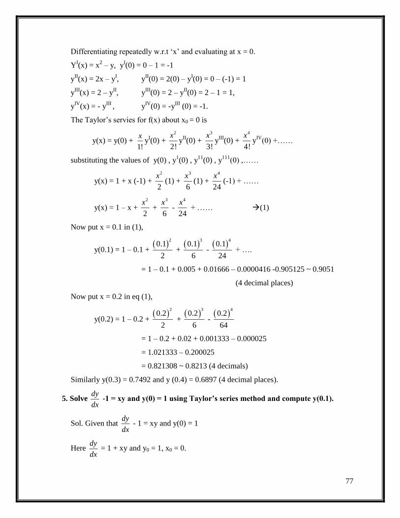
77
Differentiating repeatedly w.r.t „x‟ and evaluating at x = 0.
YI(x) = x
2 – y, y
I(0) = 0 – 1 = -1
yII(x) = 2x – y
I, y
II(0) = 2(0) – y
I(0) = 0 – (-1) = 1
yIII
(x) = 2 – yII, y
III(0) = 2 – y
II(0) = 2 – 1 = 1,
yIV
(x) = - yIII
, yIV
(0) = -yIII
(0) = -1.
The Taylor‟s servies for f(x) about x0 = 0 is
y(x) = y(0) + yI(0) + y
II(0) + y
III(0) + y
IV(0) +……
substituting the values of y(0) , y1(0) , y
11(0) , y
111(0) ,……
y(x) = 1 + x (-1) + (1) + (1) + (-1) + ……
y(x) = 1 – x + + - + …… (1)
Now put x = 0.1 in (1),
y(0.1) = 1 – 0.1 + + - + ….
= 1 – 0.1 + 0.005 + 0.01666 – 0.0000416 -0.905125 ~ 0.9051
(4 decimal places)
Now put x = 0.2 in eq (1),
y(0.2) = 1 – 0.2 + + -
= 1 – 0.2 + 0.02 + 0.001333 – 0.000025
= 1.021333 – 0.200025
= 0.821308 ~ 0.8213 (4 decimals)
Similarly y(0.3) = 0.7492 and y (0.4) = 0.6897 (4 decimal places).
5. Solve -1 = xy and y(0) = 1 using Taylor’s series method and compute y(0.1).
Sol. Given that - 1 = xy and y(0) = 1
Here = 1 + xy and y0 = 1, x0 = 0.
1!
x2
2!
x 3
3!
x 4
4!
x
2
2
x 3
6
x 4
24
x
2
2
x 3
6
x 4
24
x
2
0.1
2
3
0.1
6
4
0.1
24
2
0.2
2
3
0.2
6
4
0.2
64
dy
dx
dy
dx
dy
dx

78
Differentiating repeatedly w.r.t „x‟ and evaluating at x0 = 0
yI(x) = 1 + xy, y
I(0) = 1+0(1) = 1 .
yII(x) = x.y‟+ y, y
II(0) = 0+1=1
yIII
(x) = x.y‟‟ + yI + y
I, y
III(0) = 0.(1) + 2 (1) =2
yIV
(x) = xyIII
+ yII + 2y
II, y
IV(0) = 0+3(1) =3.
yV(x) = xy
IV + y
III +2y
III, y
V(0) = 0 + 2 + 2(3) = 8
The Taylor series for f(x) about x0 = 0 is
y(x) = y(0) + x.yI(0) + y
II (0) + y
III(0) + y
IV(0) + y
V(0)+…..
Substituting the values of y(0) , yI(0) , y
II(0) , ….
y(x) = 1 + x + + (2) + (3) + (8) + ….
y(x) = 1 + x + + + + + …. (1)
Now put x = 0.1 in equ (1),
y(0.1) = 1 + 0.1 + + + + + …..
= 1 + 0.1 +0.005 + 0.000333 + 0.0000125 + 0.0000006
= 1.1053461
H.W
6. Given the differential equ y1 = x
2 + y
2, y(0) = 1.Obtain y(0.25), and y(0.5) by
Taylor’s
Series method.
Ans: 1.3333, 1.81667
7. Solve y1
= xy2 + y, y(0) =1 using Taylor’s series method and compute y(0.1) and
y(0.2).
Ans: 1.111, 1.248.
2
2!
x 3
3!
x 4
4!
x 5
5!
x
2
2
x 3
6
x 4
24
x 5
120
x
2
2
x 3
3
x 4
8
x 5
15
x
2(0.1)
2
3(0.1)
3
4(0.1)
8
5(0.1)
15

79
Note: We know that the Taylor‟s expansion of y(x) about the point x0 in a power of (x
– x0)is.
y(x) = y(x0) + yI(x0) + y
II(x0) + y
III(x0) + … (1)
Or
y(x) = y0 + + + + …..
If we let x – x0 = h. (i.e. x = x0 + h = x1) we can write the Taylor‟s series as
y(x) = y(x1) = y0 + + + + + ….
i.e. y1 = y0 + + + + + ….. (2)
Similarly expanding y(x) in a Taylor‟s series about x = x1. We will get.
y2 = y1 + + + + + ……. (3)
Similarly expanding y(x) in a Taylor‟s series about x = x2 We will get.
y3 = y2 + + + + + …... (4)
In general, Taylor‟s expansion of y(x) at a point x= xn is
yn+1 = yn + + + + + ….. (5)
8. Solve y1
= x-y2, y(0) = 1 using Taylor’s series method and evaluate y(0.1), y(0.2).
Sol: Given y1
= x – y2 (1)
and y(0) = 1 (2)
Here x0 = 0, y0 = 1.
Differentiating (1) w.r.t „x‟, we get.
yII = 1 – 2yy
I(3)
yIII
= -2(y. yII + (y
I)2) (4)
yIV
= -2[y. yIII
+ y. yII
+ 2yI. y
II] (5)
= -2(3yI. y
II + y. y
III) …...
0( )
1!
x x2
0( )
2!
x x 3
0( )
3!
x x
0( )
1!
x x0
Iy
2
0( )
2!
x x0
IIy
3
0( )
3!
x x0
IIIy
1!
h0
Iy
2
2!
h0
IIy
3
3!
h0
IIIy
4
4!
h0
IVy
1!
h0
Iy
2
2!
h0
IIy
3
3!
h0
IIIy 04!
IVIVh
y
11!
Ihy
2
12!
IIhy
3
13!
IIIhy
4
14!
IVhy
21!
Ihy
2
22!
IIhy
3
23!
IIIhy
4
24!
IVhy
1!
I
n
hy
2
2!
II
n
hy
3
3!
III
n
hy
4
4!
IV
n
hy

80
Put x0 = 0, y0 = 1 in (1),(3),(4) and (5),
We get
= 0-1 = -1,
= 1-2(1) (-1) = 3,
= -2[(-1)2) + (1) (3)] = -8
= -2[3(-1) (3) + (1) (-8)] = -2(-9 -8) = 34.
Take h=0.1
Step1: By Taylor‟s series, we have
y1 = y0 + + + + + ….. (6)
on substituting the values of y0, , , etc in equ (6) we get
y(0.1) = y1 = 1 + (-1) + (3) + (-8) + (34) + ….
= 1 – 0.1 + 0.015 – 0.00133 + 0.00014 + …
= 0.91381
Step2: Let us find y(0.2), we start with (x1,y1) as the starting value.
Here x1 = x0 + h = 0+0.1 = 0.1 and y1 = 0.91381
Put these values of x1 and y1 in (1),(3),(4) and (5),we get
= x1 - = 0.1 – (0.91381)2 = 0.1 – 0.8350487 = -0.735
= 1 – 2y1 = 1- 2(0.91381) (-0.735) = 1 + 1.3433 = 2.3433
= - 2[( )2 + y1 ] = - 2[(-0.735)
2 + (0.91381) (2.3433)] = -5.363112
= - 2[3. + y1 ] = - 2[3.(-0.735) (2.3433) + (0.91381) (-5.363112)]
= -2[(-5.16697) – 4.9] = 20.133953
By Taylor‟s series expansion,
y2 = y1 + + + + + ….
y(0.2) = y2 = 0.91381 + (0.1) (-0.735) + (2.3433) +
0
Iy
0
IIy
0
IIIy
0
IVy
01!
Ihy
2
02!
IIhy
3
03!
IIIhy
4
04!
IVhy
0
Iy 0
IIy
0.1
1
2(0.1)
2
3(0.1)
6
4(0.1)
24
1
Iy 2
1y
1
IIy 1
Iy
1
IIIy 1
Iy 1
IIy
1
IVy 1
Iy 1
IIy 1
IIIy
11!
Ihy
2
12!
IIhy
3
13!
IIIhy
4
14!
IVhy
2(0.1)
2

81
(-5.363112) + (20.133953) + ….
y(0.2) = 0.91381 – 0.0735 + 0.0117 – 0.00089 + 0.00008
= 0.8512
9. Tabulate y(0.1), y(0.2) and y(0.3) using Taylor’s series method given that y1 = y
2 + x
and y(0) = 1
Sol: Given y1 = y
2 + x (1)
and y(0) = 1 (2)
Here x0 = 0, y0 = 1.
Differentiating (1) w.r.t „x‟, we get
= 2y yI + 1 (3)
= 2[y + (yI)2] (4)
= 2[y + yI
+ 2 yI
]
= 2[y + 3 yI
] (5)
Put x0 = 0, y0 = 1 in (1), (3), (4) and (5), we get
= (1)2 + 0 = 1
= 2(1) (1) + 1 = 3,
= 2((1) (3) + (1)2) = 8
= 2[(1)(8) + 3(1)(3)]
= 34
Take h = 0.1.
Step1: By Taylor‟s series expansion, we have
y(x1) = y1 = y0 + + + + + …. (6)
on substituting the values of yo, , etc in (6),we get
y(0.1) = y1= 1 + (0.1)(1) + (3) + (8) + (34) + ….
= 1 + 0.1 + 0.015 + 0.001333 + 0.000416
y1 = 1.116749
3(0.1)
6
4(0.1)
24
IIy
IIIy IIy
IVy IIIy IIy IIy
IIIy IIy
0
Iy
0
IIy
0
IIIy
0
IVy
01!
Ihy
2
02!
IIhy
3
03!
IIIhy
4
04!
IVhy
0
Iy 0
IIy
2(0.1)
2
3(0.1)
6
4(0.1)
24

82
Step2: Let us find y(0.2),we start with (x1,y1) as the starting values
Here x1 = x0 + h = 0 + 0.1 = 0.1 and y1 = 1.116749
Putting these values in (1),(3),(4) and (5), we get
= +x1 = (1.116749)2 + 0.1 = 1.3471283
= 2y1 + 1 = 2(10116749) (1.3471283) + 1 = 4.0088
= 2(y1 + ( )2) = 2((1.116749) (4.0088) + (1.3471283)
2] = 12.5831
= 2y1 + 6 = 2(1.116749) (12.5831) + 6(1.3471283) (4.0088) =
60.50653
By Taylor‟s expansion
y(x2) = y2 = y1 + + + + + ….
y(0.2) = y2 = 1.116749 + (0.1) (1.3471283) + (4.0088) + (12.5831)
+ (60.50653)
y2 = 1.116749 + 0.13471283 + 0.020044 + 0.002097 + 0.000252
= 1.27385
y(0.2) = 1.27385
Step3: Let us find y(0.3),we start with (x2,y2) as the starting value.
Here x2 = x1 + h = 0.1 + 0.1 =0.2 and y2 = 1.27385
Putting these values of x2 and y2 in eq (1), (3), (4) and (5), we get
= + x2 = (1.27385)2 + 0.2 = 1.82269
= 2y2 + 1 = 2(1.27385) (1.82269) + 1 = 5.64366
= 2[y2 + ( )2 ] = 2[(1.27385) (5.64366) + (1.82269)
2]
= 14.37835 + 6.64439 = 21.02274
= 2y2 + + 6 = 2(1.27385) (21.00274) + 6(1.82269) (5.64366)
= 53.559635 + 61.719856 = 115.27949
By Taylor‟s expansion,
1
Iy 2
1y
1
IIy 1
Iy
1
IIIy 1
IIy 1
Iy
1
IVy 1
IIIy 1
Iy 1
IIy
11!
Ihy
2
12!
IIhy
3
13!
IIIhy
4
14!
IVhy
2(0.1)
2
3(0.1)
6
4(0.1)
24
2
Iy 2
2y
2
IIy 1
2y
2
IIIy 2
IIy 2
Iy
2
IVy 2
IIIy 2
Iy 1
IIy

83
y(x3) = y3 = y2 + + + + + …..
y(0.3) = y3 = 1.27385 + (0.1) (1.82269) + (5.64366) + (21.02274)
+ (115.27949)
= 1.27385 + 0.182269 + 0.02821 + 0.0035037 + 0.00048033
= 1.48831
y(0.3) = 1.48831
10. Solve y1= x
2 – y, y(0) = 1 using Taylor’s series method and evaluate
y(0.1),y(0.2),y(0.3) and y(0.4) (correct to 4 decimal places)
Sol: Given y1= x
2 – y (1)
and y(0) = 1 (2)
Here x0 = 0, y0 = 1
Differentiating (1) w.r.t „x‟, we get
yII = 2x – y
1(3)
yIII
= 2- yII (4)
yIV
= -yIII (5)
put x0 = 0, y0 = 1 in (1),(3),(4) and (5), we get
= - y0 = 0-1 = -1,
= 2x0 - = 2(0) – (-1) = 1
= 2- = 2-1 = 1,
= - = -1 Take h = 0.1
Step1: by Taylor‟s series expansion
y(x1) = y1= y0 + + + + + …. (6)
On substituting the values of y0, , etc in (6), we get
y(0.1) = y1 = 1+ (0.1) (-1) + (1) + (1) + (-1)+….
21!
Ihy
2
22!
IIhy
3
23!
IIIhy
4
24!
IVhy
2(0.1)
2
3(0.1)
6
4(0.1)
24
0
Iy 2
0x
0
IIy 0
Iy
0
IIIy 0
IIy
0
IVy 0
IIIy
1!
h0
Iy
2
2!
h0
IIy
3
03!
IIIhy
4
04!
IVhy
0
Iy 0
IIy
2(0.1)
2
3(0.1)
6
4(0.1)
24

84
= 1-0.1 + 0.005 + 0.01666 – 0.0000416
= 0.905125 ~ 0.9051 (4 decimal place).
Step2: Let us find y(0.2) we start with (x1,y1) as the starting values
Here x = x0 + h = 0 + 0.1 = 0.1 and y1 = 0.905125,
Putting these values of x1 and y1 in (1), (3), (4) and (5), we get
= - y1 = (0.1)2 – 0.905125 = -0.895125
= 2x1 - = 2(0.1) – (-0.895125) = 1.095125,
= 2 - = 2 – 1.095125 = 0.90475,
= - = -0.904875,
By Taylor‟s series expansion,
y(x2) = y2 = y1 + + + + +….
y(0.2) = y2 = 0.905125 + (0.1)(-0.895125) + + (1.09125)
+ (1.095125) + (-0.904875)+….
y(0.2) = y2 = 0.905125 – 0.0895125 + 0.00547562 + 0.000150812 – 0.0000377
= 0.8212351 ~ 0.8212 (4 decimal places)
Step3: Let us find y(0.3), we start with (x2,y2) as the starting value
Here x2 = x1 + h = 0.1+ 0.1 = 0.2 and y2 = 0.8212351
Putting these values of x2 and y2 in (1),(3),(4), and (5) we get
= - y2 = (0.2)2 – 0.8212351= 0.04 – 0.8212351 = - 0.7812351
= 2x2 - = 2(0.2) + (0.7812351) = 1.1812351,
= 2 - = 2 – 1. 1812351 = 0.818765,
= - = -0.818765,
By Taylor‟s series expansion,
y(x3) = y3 = y2 + + + + +….
1
1y 2
1x
1
IIy 1
1y
1
IIIy 1
IIy
1
IVy 1
IIIy
1!
h1
Iy
2
2!
h1
IIy
3
13!
IIIhy
4
14!
IVhy
2(0.1)
23(0.1)
6
4(0.1)
24
1
2y 2
2x
2
IIy 1
2y
2
IIIy 2
IIy
2
IVy 2
IIIy
1!
h2
Iy
2
2!
h2
IIy
3
23!
IIIhy
4
24!
IVhy

85
y(0.3) = y3 = 0. 8212351 + (0.1)(-0.7812351) +
(1.1812351) + (0.818765) + (-0.818765)+….
y(0.3) = y3 = 0. 8212351– 0.07812351+ 0.005906 + 0.000136 – 0.0000034
= 0.749150 ~ 0.7492 (4 decimal places)
Step4: Let us find y(0.4), we start with (x3,y3) as the starting value
Here x3 = x2 + h = 0.2+ 0.1 = 0.3 and y3 = 0.749150
Putting these values of x3 and y3 in (1),(3),(4), and (5) we get
= - y3 = (0.3)2 – 0.749150= -0.65915,
= 2x3 - = 2(0.3) + (0.65915) = 1.25915,
= 2 - = 2 – 1. 25915 = 0.74085,
= - = -0.74085,
By Taylor‟s series expansion,
y(x4) = y4 = y3 + + + + +….
y(0.4) = y4 = 0. 749150 + (0.1)(-0.65915) + (1.25915) +
(0.74085) + (-0.74085)+….
y(0.4) = y4 = 0. 749150 – 0.065915+ 0.0062926+ 0.000123475 – 0.0000030
= 0.6896514 ~ 0.6896 (4 decimal places)
11. Solve y1 = x
2 – y, y(0) = 1using T.S.M and evaluate y(0.1),y(0.2),y(0.3) and y(0.4) (correct to
4 decimal place ) 0.9051, 0.8212, 07492, 0.6896
12. Given the differentiating equation y1 = x
1 + y
2, y(0) = 1. Obtain y(0.25) and y(0.5) by T.S.M.
Ans: 1.3333, 1.81667
13. Solve y1 = xy
2 + y, y(0) = 1 using Taylor‟s series method and evaluate y(0.1) and y(0.2)
Ans: 1.111, 1.248.
2(0.1)
23(0.1)
6
4(0.1)
24
1
3y 2
3x
3
IIy 1
3y
3
IIIy 3
IIy
3
IVy 3
IIIy
1!
h3
Iy
2
2!
h3
IIy
3
33!
IIIhy
4
34!
IVhy
2(0.1)
23(0.1)
6
4(0.1)
24

86
EULER’S METHOD
It is the simplest one-step method and it is less accurate. Hence it has a limited application.
Consider the differential equation = f(x,y) (1)
With y(x0) = y0(2)
Consider the first two terms of the Taylor‟s expansion of y(x) at x = x0
y(x) = y(x0) + (x – x0) y1(x0) (3)
from equation (1) y1(x0) = f(x0,y(x0)) = f(x0,y0)
Substituting in equation (3)
y(x) = y(x0) + (x – x0) f(x0,y0)
At x = x1, y(x1) = y(x0) + (x1 – x0) f(x0,y0)
y1 = y0 + h f(x0,y0) where h = x1 – x0
Similarly at x = x2 , y2 = y1 + h f(x1,y1),
Proceeding as above, yn+1 = yn + h f(xn,yn)
This is known as Euler‟s Method
1. Using Euler’s method solve for x = 2 from = 3x2 + 1,y(1) = 2,taking step size (I) h
= 0.5 and (II) h=0.25
Sol: here f(x,y) = 3x2 + 1, x0 = 1,y0 = 2
Euler‟s algorithm is yn+1 = yn + h f(xn,yn), n = 0,1,2,3,….. (1)
h = 0.5 x1 = x0 + h = 1+0.5 = 1.5
Taking n = 0 in (1) , we have x2 = x1 + h = 1.5 + 0.5 = 2
y1 = y0 + h f(x0,y0)
i.e. y1 = y(0.5) = 2 + (0.5) f(1,2) = 2 + (0.5) (3 + 1) = 2 + (0.5)(4)
Here x1 = x0 + h = 1 + 0.5 = 1.5
y(1.5) = 4 = y1
Taking n = 1 in (1),we have
y2 = y1 + h f(x1,y1)
dy
dx
dy
dx

87
i.e. y(x2) = y2 = 4 + (0.5) f(1.5,4) = 4 + (0.5)[3(1.5)2 + 1] = 7.875
Here x2 = x4 + h = 1.5 + 0.5 = 2
y(2) = 7.875
(I) h = 0.25 x1 = 1.25, x2 = 1.50, x3 = 1.75, x4 = 2
Taking n = 0 in (1), we have
y1 = y0 + h f(x0,y0)
i.e. y(x1) = y1 = 2 + (0.25) f(1,2) = 2 + (0.25) (3 + 1) = 3
y(x2) = y2 = y1 + h f(x1,y1)
i.e. y(x2) = y2 = 3 + (0.25) f(1.25,3)
= 3 + (0.25)[3(1.25)2 + 1]
= 4.42188
Here x2 = x1 + h = 1.25 + 0.25 = 1.5
y(1.5) = 5.42188
Taking n = 2 in (1), we have
i.e. y(x3) = y3 = h f(x2,y2)
= 5.42188 + (0.25) f(1.5,2)
= 5.42188 + (0.25) [3(1.5)2 + 1]
= 6.35938
Here x3 = x2 + h = 1.5 + 0.25 = 1.75
y(1.75) =7. 35938
Taking n = 4 in (1),we have
y(x4) = y4 = y3 + h f(x3,y3)
i.e. y(x4) = y4 = 7.35938 + (0.25) f(1.75,2)
= 7.35938 + (0.25)[3(1.75)2 + 1]
= 8.90626

88
Note that the difference in values of y(2) in both cases
(i.e. when h = 0.5 and when h = 0.25).The accuracy is improved significantly when h is
reduced to 0.25 (Example significantly of the equ is y = x3
+ x and with this y(2) = y2 = 10
2. Solve by Euler’s method,y1 = x + y, y(0) = 1 and find y(0.3) taking step size h = 0.1.
compare the result obtained by this method with the result obtained by analytical
solution
Sol: y1 = 1.1 = y(0.1),
y2 = y(0.2) = 1.22
y3 = y(0.3) = 1.362
Particular solution is y = 2ex – (x + 1)
Hence y(0.1) = 1.11034, y(0.2) = 1.3428, y(0.3) = 1.5997
We shall tabulate the result as follows
The
value of y deviate from the execute value as x increases. This indicate that the method is not
accurate
3. Solve by Euler’s method y1 + y = 0 given y(0) = 1 and find y(0.04) taking step size
h = 0.01 Ans: 0.9606
4. Using Euler’s method, solve y at x = 0.1 from y1 = x+ y +xy, y()) = 1 taking step
size h = 0.025.
5. Given that = xy ,y(0) = 1 determine y(0.1),using Euler’s method. h =0.1
Sol: The given differentiating equation is = xy, y(0) = 1
a = 0
Here f(x,y) = xy , x0 = 0 and y0 = 1
dy
dx
dy
dx
X 0
0.1
0.2
0.3
Euler y
1
1.1
1.22
1.362
Euler y
1
1.11034
1.3428
1.3997

89
Since h is not given much better accuracy is obtained by breaking up the interval (0,0.1)
in to five steps.
i.e. h = = = 0.02
Euler‟s algorithm is yn+1 = yn + h f(xn,yn) (1)
From (1) form = 0, we have
y1 = y0 +h f(x0,y0)
= 1 + (0.02) f(0,1)
= 1 + (0.02) (0)
= 1
Next we have x1 = x0 + h = 0 + 0.02 = 0.02
From (1), form = 1,we have
y2 = y1 + h f(x1,y1)
= 1 + (0.02) f(0.02,1)
= 1 + (0.02) (0.02)
= 1.0004
Next we have x2 = x1 + h = 0.02 + 0.02 =0.04
From (1), form = 2,we have
y3 = y2 + h f(x2,y2)
= 1.004 + (0.02) (0.04) (1.0004)
= 1.0012
Next we have x3 = x2 + h = 0.04 + 0.02 =0.06
From (1), form = 3,we have
y4 = y3 + h f(x3,y3)
= 1.0012 + (0.02) (0.06) (1.00012)
= 1.0024.
Next we have x4 = x3 + h = 0.06 + 0.02 =0.08
From (1), form = 4,we have
y5 = y4 + h f(x4,y4)
= 1.0024 + (0.02) (0.08) (1.00024)
= 1.0040.
5
b a 0.1
5

90
Next we have x5 = x4 + h = 0.08 + 0.02 =0.1
When x = x5, y~y5
y = 1.0040 when x = 0.1
6. Solve by Euler’s method y1 = given y(1) = 2 and find y(2).
7. Given that = 3x2 + y, y(0) = 4.Find y(0.25) and y(0.5) using Euler’s method
Sol: given = 3x2 + y and y(1) = 2.
Here f(x,y) = 3x2 + y , x0 = (1), y0 = 4
Consider h = 0.25
Euler‟s algorithm is yn+1 = yn + h f(xn,yn) (1)
From (1), for n = 0, we have
y1 = y0 + h f(x0,y0)
= 2 + (0.25)[0 + 4]
= 2 + 1
= 3
Next we have x1 = x0 + h = 0 + 0.25 = 0.25
When x = x1, y1~ y
y = 3 when x = 0.25
From (1), for n = 1, we have
y2 = y1 + h f(x1,y1)
= 3 + (0.25)[3.(0.25)2 + 3]
= 3.7968
Next we have x2 = x1 + h = 0.25 + 0.25 = 0.5
When x = x2, y ~ y2
y = 3.7968 when x = 0.5.
a. Solve first order diff equation = , y(0) = 1 and estimate y(0.1) using
Euler’s method (5 steps) Ans: 1.0928
b. Use Euler’s method to find approximate value of solution of = y-x + 5 at x = 2-1
and 2-2with initial contention y(0.2) = 1
Modified Euler’s method
It is given by
2y
x
dy
dx
dy
dx
dy
dx
y x
y x
dy
dx
1
1 1 1/ 2 , ,1 , 1,2....., 0,1.....
ii
k k k k k ky y h f x y f x i ki

91
Working rule :
i)Modified Euler’s method
ii) When can be calculated from Euler‟s method
iii) K=0, 1……… gives number of iteration.
gives number of times, a particular iteration k is repeated
Suppose consider dy/dx=f(x, y) -------- (1) with y(x0) =y0----------- (2)
To find y(x1) =y1 at x=x1=x0+h
Now take k=0 in modified Euler‟s method
We get ……………………… (3)
Taking i=1, 2, 3...k+1 in eqn (3), we get
(By Euler‟s method)
------------------------
If two successive values of are sufficiently close to one another, we will take the
common value as
We use the above procedure again
1) using modified Euler‟s method find the approximate value of when
given that
sol: Given
Here
Take h = 0.1 which is sufficiently small
Here
The formula for modified Euler‟s method is given by
Step1: To find y1= y(x1) = y (0.1)
Taking k = 0 in eqn(1)
when i = 1 in eqn (2)
1
1 1 1/ 2 , ,1 , 1,2....., 0,1.....
ii
k k k k k ky y h f x y f x i ki
1i 0
1ky
1,2...i
1 1
1 0 0 0 1 1/ 2 , ,i
y y h f x y f x y
0
1 0 0 0/ 2 ,y y h f x y
1 0
1 0 0 0 1 1/ 2 , ,y y h f x y f x y
2 1
1 0 0 0 1 1/ 2 , ,y y h f x y f x y
1
1 0 0 0 1 1/ 2 , ,k k
y y h f x y f x y
1
1 1,k k
y y
2 2 1y y x y x h
x 0.3x
/ 0 1dy dx x y and y
/ 0 1dy dx x y and y
0 0, , 0, 1f x y x y x and y
0 1 0 2 1 3 20, 0.1, 0.2, 0.3x x x h x x h x x h
1
1 1 1/ 2 , 1i i
k k k k k ky y h f x y f x y
1
1 0 0 0 1 1/ 2 , 2i i
ky y h f x y f x y

92
First apply Euler‟s method to calculate = y1
= 1+(0.1)f(0.1)
= 1+(0.1)
= 1.10
= 1+0.1/2[f(0,1) + f(0.1,1.10)
= 1+0.1/2[(0+1)+(0.1+1.10)]
= 1.11
When i=2 in eqn (2)
= 1+0.1/2[f(0.1)+f(0.1,1.11)]
= 1 + 0.1/2[(0+1)+(0.1+1.11)]
= 1.1105
= 1+0.1/2[f(0,1)+f(0.1 , 1.1105)]
= 1+0.1/2[(0+1)+(0.1+1.1105)]
= 1.1105
Since
y1 = 1.1105
Step:2 To find y2 = y(x2) = y(0.2)
Taking k = 1 in eqn (1) , we get
i = 1,2,3,4,…..
For i = 1
0
1 0 0 0 1 1/ 2 , ,i
y y h f x y f x y
(0)
1y
0
1 0 0 0,y y h f x y
0 0 1 10, 1, 0.1, 0 1.10now x y x y
1 0
1 0 0 0 1 10.1/ 2 , ,y y f x y f x y
2 1
1 0 0 0 1 1/ 2 , ,y y h f x y f x y
3 2
1 0 0 0 1 1/ 2 , ,y y h f x y f x y
2 3
1 1y y
1
2 1 1 1 2 2/ 2 , , 3i i
y y h f x y f x y
1 0
2 1 1 1 2 2/ 2 , ,y y h f x y f x y
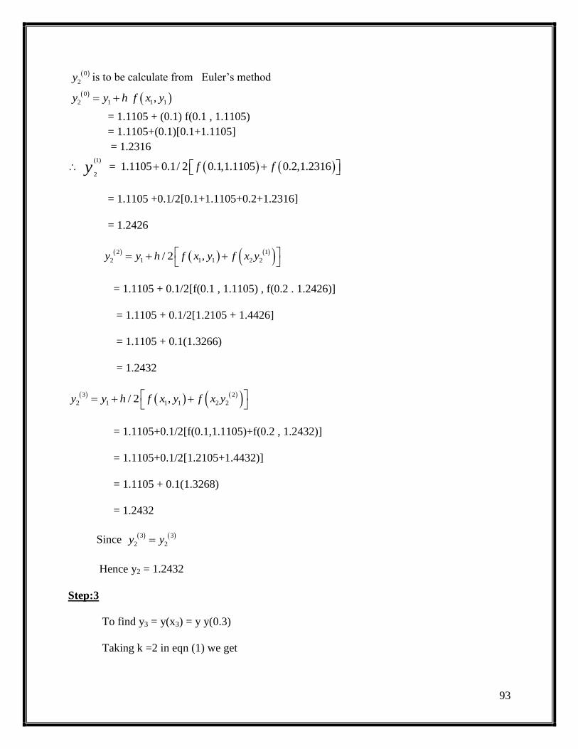
93
is to be calculate from Euler‟s method
= 1.1105 + (0.1) f(0.1 , 1.1105)
= 1.1105+(0.1)[0.1+1.1105]
= 1.2316
=
= 1.1105 +0.1/2[0.1+1.1105+0.2+1.2316]
= 1.2426
= 1.1105 + 0.1/2[f(0.1 , 1.1105) , f(0.2 . 1.2426)]
= 1.1105 + 0.1/2[1.2105 + 1.4426]
= 1.1105 + 0.1(1.3266)
= 1.2432
= 1.1105+0.1/2[f(0.1,1.1105)+f(0.2 , 1.2432)]
= 1.1105+0.1/2[1.2105+1.4432)]
= 1.1105 + 0.1(1.3268)
= 1.2432
Since
Hence y2 = 1.2432
Step:3
To find y3 = y(x3) = y y(0.3)
Taking k =2 in eqn (1) we get
0
2y
0
2 1 1 1,y y h f x y
(1)
2y 1.1105 0.1/ 2 0.1,1.1105 0.2,1.2316f f
2 1
2 1 1 1 2 2/ 2 ,y y h f x y f x y
3 2
2 1 1 1 2 2/ 2 ,y y h f x y f x y
3 3
2 2y y

94
For i = 1 ,
is to be evaluated from Euler‟s method .
= 1.2432 +(0.1) f(0.2 , 1.2432)
= 1.2432+(0.1)(1.4432)
= 1.3875
= 1.2432+0.1/2[f(0.2 , 1.2432)+f(0.3, 1.3875)]
= 1.2432 + 0.1/2[1.4432+1.6875]
= 1.2432+0.1(1.5654)
= 1.3997
= 1.2432+0.1/2[1.4432+(0.3+1.3997)]
= 1.2432+ (0.1) (1.575)
= 1.4003
= 1.2432+0.1/2[f(0.2 , 1.2432)+f(0.3 , 1.4003)]
= 1.2432 + 0.1(1.5718)
= 1.4004
1 1
3 2 2 2 3 3/ 2 , , 4i
y y h f x y f x y
1 0
3 2 2 2 3 3/ 2 , ,y y h f x y f x y
0
3y
0
3 2 2 2,y y h f x y
1
3y
2 1
3 2 2 2 3 3/ 2 , ,y y h f x y f x y
3 2
3 2 2 2 3 3/ 2 , ,y y h f x y f x y
4 3
3 2 2 2 3 3/ 2 , ,y y h f x y f x y

95
= 1.2432 + 0.1/2[1.4432+1.7004]
= 1.2432+(0.1)(1.5718)
= 1.4004
Since
Hence The value of y at x = 0.3 is 1.4004
2 . Find the solution of = x-y , y(0)=1 at x =0.1 , 0.2 ,0.3 , 0.4 and 0.5 . Using modified
Euler’s method
Sol . Given = x-y and y(0) = 1
Here f(x,y) = x-y , x0 = 0 and y0 = 1
Consider h = 0.1 so that
x = 0.1 , x2 = 0.2 , x3 =0.3 , x4 = 0.4 and x5 = 0.5
The formula for modified Euler‟s method is given by
Where k = 0,1, 2, 3,….. i = 1, 2, 3,…..
3. Find y(0.1) and y(0.2) using modified Euler‟s formula given that dy/dx=x2-y,y(0)=1
[consider h=0.1,y1=0.90523,y2=0.8214]
4. Given compute y(0.2) in steps of 0.1
Using modified Euler‟s method
[h=0.1, y1=1.9804, y2=1.9238]
5. Given y1
= x+siny, y(0)=1 compute y(0.2) and y(0.4) with h=0.2 using modified Euler‟s
method
[y1=1.2046, y2=1.4644]
Runge – Kutta Method
3 4
3 3y y
3 1.4004y
dy
dx
dy
dx
1
1 1 1/ 2 , , 1i i
k k k k k ky y h f x y fx y
2/ , 0 2dy dx xy y

96
I. Second order R-K Formula
yi+1 = yi+1/2 (K1+K2),
Where K1 = h (xi, yi)
K2 = h (xi+h, yi+k1)
For i= 0,1,2-------
II. Third order R-K Formula
yi+1 = yi+1/6 (K1+4K2+ K3),
Where K1 = h (xi, yi)
K2 = h (xi+h/2, y0+k1/2)
K3 = h (xi+h, yi+2k2-k1)
For i= 0,1,2-------
III. Fourth order R-K Formula
yi+1 = yi+1/6 (K1+2K2+ 2K3+K4),
Where K1 = h (xi, yi)
K2 = h (xi+h/2, yi+k1/2)
K3 = h (xi+h/2, yi+k2/2)
K4 = h (xi+h, yi+k3)
For i= 0,1,2-------
1. Using Runge-Kutta method of second order, find from = , y(2)=2 , h =
0.25 .
Sol: Given = , y(2) = 2 .
Here f(x, y) = , x0 = 0 , y0=2 and h = 0.25
2.5ydy
dx
x y
x
dy
dx
x y
x
x y
x
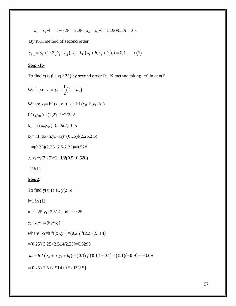
97
x1 = x0+h = 2+0.25 = 2.25 , x2 = x1+h =2.25+0.25 = 2.5
By R-K method of second order,
Step -1:-
To find y(x1)i.e y(2.25) by second order R - K method taking i=0 in eqn(i)
We have
Where k1= hf (x0,y0 ), k2= hf (x0+h,y0+k1)
f (x0,y0 )=f(2,2)=2+2/2=2
k1=hf (x0,y0 )=0.25(2)=0.5
k2= hf (x0+h,y0+k1)=(0.25)f(2.25,2.5)
=(0.25)(2.25+2.5/2.25)=0.528
y1=y(2.25)=2+1/2(0.5+0.528)
=2.514
Step2:
To find y(x2) i.e., y(2.5)
i=1 in (1)
x1=2.25,y1=2.514,and h=0.25
y2=y1+1/2(k1+k2)
where k1=h f((x1,y1 )=(0.25)f(2.25,2.514)
=(0.25)[2.25+2.514/2.25]=0.5293
=(0.25)[2.5+2.514+0.5293/2.5]
1 1 2 1 11/ 2 , , , 0,1.... 1i i i iy y k k k hf x h y k i
1 0 1 2
1
2y y k k
2 0 0 1, 0.1 0.1,1 0.1 0.1 0.9 0.09k h f x h y k f

98
=0.55433
(2.5)=2.514+1/2(0.5293+0.55433)
=3.0558
y =3.0558 when x = 2.5
Obtain the values of y at x=0.1,0.2 using R-K method of
(i)second order (ii)third order (iii)fourth order for the diff eqn y1+y=0,y(0)=1
Sol: Given dy/dx = -y, y(0)=1
f(x,y) = -y, x0 = 0, y0 = 1
Here f (x,y) = -y, x0 = 0, y0 = 1 take h = 0.1
x1 = x0+h = 0.1,
x2 = x1+h = 0.2
Second order:
step1: To find y(x1) i.e y(0.1) or y1
by second-order R-K method,we have
y1 = y0+1/2(k1+k2)
where k1=hf(x0,y0)=(0.1) f(0,1) = (0.1)(-1)= - 0.1
k2= hf (x0+h, y0+k1)= (0.1) f (0.1, 1-0.1) = (0.1)(-0.9) = -0.09
y1=y(0.1)=1+1/2(-0.1-0.09)=1-0.095=0.905
y =0.905 when x=0.1
Step2:
To find y2 i.e y(x2) i.e y(0.2)
Here x1 = 0.1, y1 = 0.905 and h=0.1
By second-order R-K method, we have
2y y

99
y2 = y(x2)= y1+1/2(k1+k2)
Where =(0.1)f(0.1,0.905)=(0.1)(-0.905)=-0.0905
y2 = y(0.2)=0.905+1/2(-0.0905-0.08145)
= 0.905- 0.085975 = 0819025
Third order
Step1:
To find y1 i.e y(x1)= y(0.1)
By Third order Runge kutta method
where k1 = h f(x0, y0) = (0.1) f (0.1) = (0.1) (-1) = -0.1
and k3 = h f((x0+h,y0+2k2-k1)
(0.1) f (0.1,1+2(-0.095)+0.1)= -0.905
Hence y1 = 1+1/6(-0.1+4(-0.095)-0.09) = 1+1/6 (-0.57) = 0.905
y1=0.905 i.e y(0.1)= 0.905
Step2:
To find y2,i.e y(x2)= y(0.2)
Here x1=0.1,y1=0.905 and h = 0.1
Again by 2nd
order R-K method
1 1 1,k h f x y
2 1 1 1, 0.1 0.2,0.905 0.0905
0.1 0.2,0.8145 0.1 0.8145
0.08145
k h f x h y k f
f
1 0 1 2 31/ 6 4y y k k k
2 0 0 1/ 2, / 2 0.1 0.1/ 2,1 0.1/ 2 0.1 0.05,0.95
0.1 0.95 0.095
k h f x h y k f f

100
y2 = y1+1/6(k1+4k2+k3)
Where k1=h f(x1, y1) = (0.1)f (0.1,0.905)= -0.0905
k2 = h f (x1+h/2,y1+k1/2)=(0.1)f(0.1+0.2,0.905 - 0.0905)= -(0.1) f (0.15, 0.85975)= (0.1) (-
0.85975)
and k3 = h f((x1+h,y1+2k2-k1)=(0.1)f(0.2,0.905+2(0.08975)+0.0905= -0.082355
hence y2 = 0.905+1/6(-0.0905+4(-0.085975)-0.082355)=0.818874
y = 0.905 when x = 0.1
And y =0.818874 when x =0.2
fourth order:
step1:
x0=0,y0=1,h=0.1 To find y1 i.e y(x1)=y(0.1)
By 4th
order R-K method, we have
y1 = y0+1/6(k1+2k2+2k3+k4)
Where k1=h f(x0,y0)=(0.1)f(0.1)= -0.1
k2= h f (x0+h/2, y0+k1/2) = -0.095
and k3= h f((x0+h/2,y0+k2/2)=(0.1)f (0.1/2,1-0.095/2)
= (0.1)f(0.05,0.9525)
= -0.09525
and k4= h f(x0+h,y0+k3)
= (0.1) f(0.1,1-0.09525)=(0.1)f(0.1,0.90475)
=-0.090475
Hence y1=1+1/6(-0.1)+2(-0.095)+2(0.09525)-0.090475)
=1+1/6(-0.570975)+1-0.951625 = 0.9048375
Step2:
To find
2 2 1, . ., 0.2 , 0.9048375, . ., 0.1 0.9048375y i e y x y y i e y

101
Here x1 = 0.1, y1=0.9048375 and h = 0.1
Again by 4th
order R-K method, we have
y2 = y1+1/6(k1+2k2+2k3+k4)
Where k1=h f(x1,y1)=(0.1)f(0.1,0.9048375)=-0.09048375
k2= hf (x1+h/2,y1+k1/2)=(0.1)f(0.1+0.1/2,0.9048375 -0.09048375 /2)=-0.08595956
and k3=hf(x1+h/2, y1+k2/2)=(0.1)f(0.15,0. 8618577)= -0.08618577
k4 =h f(x1+h,y1+k3)=(0.1)f(0.2,0.86517)
= -0.08186517
Hence y2 = 0.09048375+1/6(-0.09048375-2(0.08595956)-2(0.08618577)- 0.08186517
=0.9048375-0.0861065
=0.818731
y = 0.9048375 when x =0.1 and y =0.818731
3. Apply the 4th
order R-K method to find an approximate value of y when x=1.2 in steps
of 0.1,given that
y1
= x2+y
2,y (1)=1.5
sol. Given y1= x
2+y
2,and y(1)=1.5
Here f(x,y)= x2+y
2, y0 =1.5 and x0=1,h=0.1
So that x1=1.1 and x2=1.2
Step1:
To find y1 i.e., y(x1)
by 4th
order R-K method we have
y1=y0+1/6 (k1+2k2+2k3+k4)
k1=hf(x0,y0)=(0.1)f(1,1.5)=(0.1) [12+(1.5)
2]=0.325

102
k2= hf (x0+h/2,y0+k1/2)=(0.1)f(1+0.05,1.5+0.325)=0.3866
and k3=hf((x0+h/2,y0+k2/2)=(0.1)f(1.05,1.5+0. 3866/2)=(0.1)[(1.05)2+(1.6933)
2]
=0.39698
k4=hf(x0+h,y0+k3)=(0.1)f(1.0,1.89698)
=0.48085
Hence
Step2:
To find y2, i.e.,
Here x1=0.1,y1=1.8955 and h=0.1
by 4th
order R-K method we have
y2 = y1+1/6(k1+2k2+2k3+k4)
k1=hf(x1,y1)=(0.1)f(0.1,1.8955)=(0.1) [12+(1.8955)
2]=0.48029
k2= hf (x1+h/2,y1+k1/2)=(0.1)f(1.1+0.1,1.8937+0.4796) =0.58834
and k3=hf((x1+h/2,y1+k2/2)=(0.1)f(1.5,1.8937+0.58743) =(0.1)[(1.05)2+(1.6933)
2]
=0.611715
k4=hf(x1+h,y1+k3)=(0.1)f(1.2,1.8937+0.610728)
=0.77261
Hence y2=1.8937+1/6(0.4796+2(0.58834)+2(0.611715)+0.7726) =2.5043
y =2.5043 where
4. using R-K method, find y(0.2) for the eqn dy/dx=y-x,y(0)=1,take h=0.2
Ans:1.15607
1
11.5 0.325 2 0.3866 2 0.39698 0.48085
6
1.8955
y
2 1.2y x y
0.2x

103
5.Given that y1=y-x,y(0)=2 find y(0.2) using R- K method take h=0.1
Ans: 2.4214
6. Apply the 4th
order R-K method to find for one equation
take h = 0.1 Ans. 1.0207, 1.038
7. using R-K method, estimate y(0.2) and y(0.4) for the eqn dy/dx=y2-x
2/ y
2+x
2,y(0)=1,h=0.2
Ans:1.19598,1.3751
8. use R-K method, to approximate y when x=0.2 given that y1=x+y,y(0)=1
Sol: Here f(x,y)=x+y,y0=1,x0=0
Since h is not given for better approximation of y
Take h=0.1
x1=0.1, x2=0.2
Step1
To find y1 i.e y(x1)=y(0.1)
By R-K method,we have
y1=y0+1/6 (k1+2k2+2k3+k4)
Where k1=hf(x0,y0)=(0.1)f(0,1)=(0.1) (1)=0.1
k2= hf (x0+h/2,y0+k1/2)=(0.1)f(0.05,1.05)=0.11
and k3=hf((x0+h/2,y0+k2/2)=(0.1)f(0.05,1+0. 11/2)=(0.1)[(0.05) +(4.0.11/2)]
=0.1105
k4=h f (x0+h,y0+k3)=(0.1)f(0.1,1.1105)=(0.1)[0.1+1.1105]
=0.12105
0.2 0.4y and y
2 210 , 0 1dy
x y ydx

104
Hence
y = 1.11034
Step2:
To find y2 i.e y(x2) = y(0.2)
Here x1=0-1, y1=1.11034 and h=0.1
Again By R-K method,we have
y2=y1+1/6(k1+2k2+2k3+k4)
k1=h f(x1,y1)=(0.1)f(0.1,1.11034)=(0.1) [1.21034]=0.121034
k2= h f (x1+h/2, y1+k1/2)=(0.1)f(0.1+0.1/2,1.11034+0.121034/2)
=0.1320857
and k3=h f((x1+h/2,y1+k2/2)=(0.1)f(0.15,1.11034+0.1320857/2)
=0.1326382
k4=h f(x1+h,y1+k3)=(0.1)f(0.2,1.11034+0.1326382)
(0.1)(0.2+1.2429783)=0.1442978
Hence y2=1.11034+1/6(0.121034+0.2641714+0.2652764+0.1442978
=1.11034+0.1324631 =1.242803
y =1.242803 when x=0.2
9.using Runge-kutta method of order 4,compute y(1.1) for the eqn y1=3x+y
2,y(1)=1.2 h = 0.05
Ans:1.7278
10. using Runge-kutta method of order 4,compute y(2.5) for the eqn dy/dx = x+y/x, y(2)=2
[hint h = 0.25(2 steps)]
Ans:3.058
1
10.1 1 0.1 0.22 0.240 0.12105
6y y

105
MODULE – V
PARTIAL DIFFERENTIAL EQUATIONS AND APPLICATIONS
Introduction
The concept of a differential equation to include equations that involve partial derivatives, not
just ordinary ones. Solutions to such equations will involve functions not just of one variable,
but of several variables. Such equations arise naturally, for example, when one is working with
situations that involve positions in space that vary over time. To model such a situation, one
needs to use functions that have several variables to keep track of the spatial dimensions and an
additional variable for time.
Examples of some important PDEs:
(1) 2
22
2
2
x
uc
t
u
One-dimensional wave equation
(2) 2
22
x
uc
t
u
One-dimensional heat equation
(3) 02
2
2
2
y
u
x
u Two-dimensional Laplace equation
(4) ),(2
2
2
2
yxfy
u
x
u
Two-dimensional Poisson equation
Partial differential equations: An equation involving partial derivatives of one dependent
variable with respective more than one independent variables.
Notations which we use in this unit:
𝑝 =𝜕𝑧
𝜕𝑥 ,𝑞 =
𝜕𝑧
𝜕𝑦, 𝑟 =
𝜕2𝑧
𝜕𝑥 2, =𝜕2𝑧
𝜕𝑥 𝜕𝑦 , t=
𝜕2𝑧
𝜕𝑦 2 ,
Formation of partial differential equation:
A partial differential equation of given curve can be formed in two ways
1. By eliminating arbitrary constants
2. By eliminating arbitrary functions
Problems
1 Form a partial differential equation by eliminating a,b,c from

106
𝒙𝟐
𝒂𝟐+
𝒚𝟐
𝒃𝟐+
𝒛𝟐
𝒄𝟐= 𝟏
Sol Given 𝑥2
𝑎2 +𝑦2
𝑏2 +𝑧2
𝑐2 = 1
Differentiating partially w.r.to x and y, we have 1
𝑎2 2𝑥 +
1
𝑐2 (2𝑧)𝜕𝑧
𝜕𝑥=o
1
𝑎2 𝑥 +
1
𝑐2 (𝑧) 𝑝 =o _______(1)
And 1
𝑏2 2𝑥 +
1
𝑐2 (2𝑧)𝜕𝑧
𝜕𝑥=o
1
𝑏2 𝑦 +
1
𝑐2 (𝑧) q = o _______(2)
Diff (1) partially w.r.to x, we have 1
𝑎2 +𝑝
𝑐2
𝜕𝑧
𝜕𝑥+
𝑧
𝑐2
𝜕𝑝
𝜕𝑥=o ______(3)
1
𝑎2 +𝑝2
𝑐2 +𝑧
𝑐2 𝑟 =O
Multiply this equation by x and then subtracting (1) from it
1
𝑐2 𝑥𝑧𝑟 + 𝑥𝑝2 − 𝑝𝑧 = 0
2 Form a partial differential equation by eliminating the constants from
(𝒙 − 𝒂)𝟐 + (𝒚 − 𝒃)𝟐 = 𝒛𝟐𝒄𝒐𝒕𝟐α, where α is a parameter
Sol Given (𝑥 − 𝑎)2 + (𝑦 − 𝑏)2 = 𝑧2𝑐𝑜𝑡2α ___________(1)
Differentiating partially w.r.to x and y, we have
2 (𝑥 − 𝑎)+0 = 2 z p𝑐𝑜𝑡2𝛼
(𝑥 − 𝑎) = Zp𝑐𝑜𝑡2𝛼
And 0+2(y-b) = 2zq𝑐𝑜𝑡2𝛼
(Y-b) = zq𝑐𝑜𝑡2𝛼
Substituting the values of (x-a) and (y-b) in (1),we get
(𝑧𝑝𝑐𝑜𝑡2𝛼)2 + (𝑧𝑞𝑐𝑜𝑡2𝛼)2 = 𝑧2𝑐𝑜𝑡2𝛼
𝑝2 + 𝑞2 (𝑐𝑜𝑡2𝛼)2 = 𝑐𝑜𝑡2𝛼
𝑝2 + 𝑞2 = 𝑡𝑎𝑛2𝛼
3 Form the partial differential equation by eliminating a and b from
log (az-1)=x+ay+b
Sol Given equation is
Log (az-1)=x+ay+b

107
Differentiating partially w.r.t. x and y ,we get 1
𝑎𝑧−1 𝑎𝑝 = 1 ⟹ 𝑎𝑝 = 𝑎𝑧 − 1 --------------- (1)
1
𝑎𝑧−1 𝑎𝑞 = 𝑎 ⟹ 𝑎𝑞 = 𝑎 𝑎𝑧 − 1 ------------- (2)
(2)/(1) gives 𝑞
𝑝= 𝑎 𝑜𝑟 𝑎𝑝 = 𝑞---------------- (3)
Substituting (3) in (1), we get
𝑞 =𝑞
𝑝. (𝑧 − 1)
i.e. pq=qz-p
𝑝 𝑞 + 1 = 𝑞𝑧
4 Find the differential equation of all spheres whose centers lie on z-axis
with a given radius r.
Sol The equation of the family of spheres having their centers on z-axis and having
radius r is
𝑥2 + 𝑦2 + (𝑧 − 𝑐)2 = 𝑟2
Where c and r are arbitrary constants
Differentiating this eqn partially w.r.t. x and y ,we get
2𝑥 + 2 𝑧 − 𝑐 𝜕𝑧
𝜕𝑥= 0 ⇒ 𝑥 + 𝑧 − 𝑐 𝑝 = 0 _________(1)
2𝑦 + 2 𝑧 − 𝑐 𝜕𝑧
𝜕𝑦= 0 ⟹ 𝑦 + 𝑧 − 𝑐 𝑞 = 0_________(2)
From (1), 𝑧 − 𝑐 = −𝑥
𝑝 ___________(3)
From (2), 𝑧 − 𝑐 = −𝑦
𝑞 ___________(4)
From (3) and (4)
We get −𝑥
𝑝 = −
𝑦
𝑞
i.e. 𝑥𝑞 − 𝑦𝑝 = 0
Linear partial differential equations of first order :
Lagrange’s linear equation: An equation of the form Pp + Qq = R is called Lagrange‟s linear
equation.
To solve Lagrange‟s linear equation consider auxiliary equation 𝑑𝑥
𝑃 =
𝑑𝑦
𝑄 =
𝑑𝑧
𝑅
Problems
1 solve 𝒙𝟐 − 𝒚𝟐 − 𝒚𝒛 𝒑 + 𝒙𝟐 − 𝒚𝟐 − 𝒛𝒙 𝒒 = 𝒛(𝒙 − 𝒚)
Sol Here
P= x2 − y2 − yz , Q = x2 − y2 − zx , R = z(x − y)

108
The subsidiary equations are dx
x2−y2−yz =
dy
x2−y2−zx =
dz
z(x−y)
Using 1,-1,0 and x,-y,0 as multipliers , we have
. dz
z x−y =
dx−dy
z x−y =
x dx−ydy
x2−y2)(x−y
From the first two rations 0f ,we have
dz= dx-dy
integrating , z=x-y-c1 or x-y-z = c1
now taking first and last ratios in (2) ,we get
dz
z=
x dx − y dy
x2 − y2 or
2dz
z=
2x dx − 2y dy
x2 − y2
Integrating ,2 log z = log x2 − y2 − logc2
⟹x2 − y2
z2= c2
The required general solution is f x − y − z ,x2−y2
z2 = 0
5 Find the general solution of the first-order linear partial differential equation
with the constant coefficients: 4ux+uy=x2y
Sol The auxiliary system of equations is
yx
du
1
dy
4
dx2
From here we get
1
dy
4
dx or dx-4dy=0. Integrating both sides
we get x-4y=c. Also yx
du
4
dx2
or x2y dx=4du
or x2
dx)4
c-x( =4du or
16
1 (x
3 – cx
2) dx = du
Integrating both sides we get
u=c1+ 192
cx4-x3 34
= f(c)+ 192
cx4-x3 34
After replacing c by x-4y, we get the general solution
u=f(x-4y)+ 192
x)y4-x(4-x3 34

109
=f(x-4y)- 12
yx
192
x 34
6 Find the general solution of the partial differential equation y2up + x
2uq = y
2x
Sol The auxiliary system of equations is
222 xy
du
ux
dy
uy
dx
Taking the first two members we have x2dx = y
2dy which on integration
given x3-y
3 = c1. Again taking the first and third members,
we have x dx = u du
which on integration given x2-u
2 = c2
Hence, the general solution is
F(x3-y
3,x
2-u
2) = 0
7 Find the general solution of the partial differential equation.
0-
22
uy
y
ux
x
u
Sol : Let p =
x
u
, q =
y
u
The auxiliary system of equations is
2222 q-q
dq
p-p
dp
)yqxp(2
du
qy2
dy
px2
dx
which we obtain from putting values of
22 qy
F,1-
u
F,p
x
F,qy2
q
F,px2
p
F
and multiplying by -1 throughout the auxiliary system. From first and 4th
expression
in (11.38) we get
dx = py
pxdp2dxp2 . From second and 5
th expression
dy= qy
qydq2dyq2
Using these values of dx and dy we get
xp
pxdp2dxp2
2 =
yq
qydq2dyq2
2
or q
dq2
y
dydp
p
2
x
dx
Taking integral of all terms we get

110
ln|x| + 2ln|p| = ln|y|+2ln|q|+lnc
or ln|x| p2 = ln|y|q
2c
or p2x=cq
2y, where c is an arbitrary constant.
Solving for p and q we get cq2y+q
2y -u=0
(c+1)q2y=u
q=2
1
y)1c(
u
p= 2
1
x)1c(
cu
du= dyy)1c(
udx
x)1c(
cu 21
21
or dyy
idx
x
cdu
u
c1 21
21
21
By integrating this equation we obtain 12
12
12
1
c)y()cx()u)c1((
This is a complete solution.
8 Solve p2+q
2=1
Sol The auxiliary system of equation is
-0
dq
0
dp
q2-p2-
du
q2
dy
p2-
dx22
or 0
dq
0
dp
qp
du
q
dy
p
dx22
Using dp =0, we get p=c and q=2c-1 , and these two combined with du
=pdx+qdy yield
u=cx+y2c-1 + c1 which is a complete solution.
Using du
dx = p , we get du =
c
dx where p= c
Integrating the equation we get u = c
x + c1
Also du = q
dy, where q =
22 c-1p-1
or du = 2c-1
dy. Integrating this equation we get u =
2c-1
1 y +c2
This cu = x+cc1 and 2c-1u = y + c2
2c-1
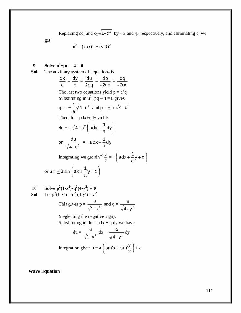
111
Replacing cc1 and c22c-1 by - and - respectively, and eliminating c, we
get
u2 = (x-)
2 + (y-)
2
9 Solve u2+pq – 4 = 0
Sol The auxiliary system of equations is
q
dx =
p
dy =
pq2
du =
up2-
dp =
uq2-
dq
The last two equations yield p = a2q.
Substituting in u2+pq – 4 = 0 gives
q = 2u-4a
1 and p = + a
2u-4
Then du = pdx+qdy yields
du = +
dy
a
1adxu-4 2
or 2u-4
du = + dy
a
1adx
Integrating we get sin--1
2
u = +
cy
a
1adx
or u = + 2 sin
cy
a
1ax
10 Solve p2(1-x
2)-q
2(4-y
2) = 0
Sol Let p2(1-x
2) = q
2 (4-y
2) = a
2
This gives p = 2x-1
a and q =
2y-4
a
(neglecting the negative sign).
Substituting in du = pdx + q dy we have
du = 2x-1
adx +
2y-4
ady
Integration gives u = a
2
ysin' x sin' + c.
Wave Equation

112
For the rest of this introduction to PDEs we will explore PDEs representing some of the basic
types of linear second order PDEs: heat conduction and wave propagation. These represent two
entirely different physical processes: the process of diffusion, and the process of oscillation,
respectively. The field of PDEs is extremely large, and there is still a considerable amount of
undiscovered territory in it, but these two basic types of PDEs represent the ones that are in some
sense, the best understood and most developed of all of the PDEs. Although there is no one way
to solve all PDEs explicitly, the main technique that we will use to solve these various PDEs
represents one of the most important techniques used in the field of PDEs, namely separation of
variables (which we saw in a different form while studying ODEs). The essential manner of
using separation of variables is to try to break up a differential equation involving several partial
derivatives into a series of simpler, ordinary differential equations.
We start with the wave equation. This PDE governs a number of similarly related phenomena,
all involving oscillations. Situations described by the wave equation include acoustic waves,
such as vibrating guitar or violin strings, the vibrations of drums, waves in fluids, as well as
waves generated by electromagnetic fields, or any other physical situations involving
oscillations, such as vibrating power lines, or even suspension bridges in certain circumstances.
In short, this one type of PDE covers a lot of ground.
We begin by looking at the simplest example of a wave PDE, the one-dimensional wave
equation. To get at this PDE, we show how it arises as we try to model a simple vibrating string,
one that is held in place between two secure ends. For instance, consider plucking a guitar string
and watching (and listening) as it vibrates. As is typically the case with modeling, reality is quite
a bit more complex than we can deal with all at once, and so we need to make some simplifying
assumptions in order to get started.
First off, assume that the string is stretched so tightly that the only real force we need to consider
is that due to the string‟s tension. This helps us out as we only have to deal with one force, i.e.
we can safely ignore the effects of gravity if the tension force is orders of magnitude greater than
that of gravity. Next we assume that the string is as uniform, or homogeneous, as possible, and
that it is perfectly elastic. This makes it possible to predict the motion of the string more readily
since we don‟t need to keep track of kinks that might occur if the string wasn‟t uniform. Finally,
we‟ll assume that the vibrations are pretty minimal in relation to the overall length of the string,
i.e. in terms of displacement, the amount that the string bounces up and down is pretty small.
The reason this will help us out is that we can concentrate on the simple up and down motion of
the string, and not worry about any possible side to side motion that might occur.
Now consider a string of a certain length, l, that‟s held in place at both ends. First off, what
exactly are we trying to do in “modeling the string‟s vibrations”? What kind of function do we
want to solve for to keep track of the motion of string? What will it be a function of? Clearly if

113
the string is vibrating, then its motion changes over time, so time is one variable we will want to
keep track of. To keep track of the actual motion of the string we will need to have a function
that tells us the shape of the string at any particular time. One way we can do this is by looking
for a function that tells us the vertical displacement (positive up, negative down) that exists at
any point along the string – how far away any particular point on the string is from the
undisturbed resting position of the string, which is just a straight line. Thus, we would like to
find a function ),( txu of two variables. The variable x can measure distance along the string,
measured away from one chosen end of the string (i.e. x = 0 is one of the tied down endpoints of
the string), and t stands for time. The function ),( txu then gives the vertical displacement of the
string at any point, x, along the string, at any particular time t.
As we have seen time and time again in calculus, a good way to start when we would like to
study a surface or a curve or arc is to break it up into a series of very small pieces. At the end of
our study of one little segment of the vibrating string, we will think about what happens as the
length of the little segment goes to zero, similar to the type of limiting process we‟ve seen as we
progress from Riemann Sums to integrals.
Suppose we were to examine a very small length of the vibrating string as shown in figure 1:
Now what? How can we figure out what is happening to the vibrating string? Our best hope is
to follow the standard path of modeling physical situations by studying all of the forces involved
and then turning to Newton‟s classic equation maF . It‟s not a surprise that this will help us,
as we have already pointed out that this equation is itself a differential equation (acceleration
being the second derivative of position with respect to time). Ultimately, all we will be doing is
substituting in the particulars of our situation into this basic differential equation.
Because of our first assumption, there is only one force to keep track of in our situation, that of
the string tension. Because of our second assumption, that the string is perfectly elastic with no
kinks, we can assume that the force due to the tension of the string is tangential to the ends of the
small string segment, and so we need to keep track of the string tension forces 1T and 2T at each
end of the string segment. Assuming that the string is only vibrating up and down means that the
horizontal components of the tension forces on each end of the small segment must perfectly
balance each other out. Thus

114
(1) TTT coscos 21
whereT is a string tension constant associated with the particular set-up (depending, for instance,
on how tightly strung the guitar string is). Then to keep track of all of the forces involved means
just summing up the vertical components of 1T and 2T . This is equal to
(2) sinsin 12 TT
where we keep track of the fact that the forces are in opposite direction in our diagram with the
appropriate use of the minus sign. That‟s it for “Force,” now on to “Mass” and “Acceleration.”
The mass of the string is simple, just x , where is the mass per unit length of the string, and
x is (approximately) the length of the little segment. Acceleration is the second derivative of
position with respect to time. Considering that the position of the string segment at a particular
time is just ),( txu , the function we‟re trying to find, then the acceleration for the little segment is
2
2
t
u
(computed at some point between a and a + x ). Putting all of this together, we find that:
(3) 2
2
12 sinsint
uxTT
Now what? It appears that we‟ve got nowhere to go with this – this looks pretty unwieldy as it
stands. However, be sneaky… try dividing both sides by the various respective equal parts
written down in equation (1):
(4) 2
2
1
1
2
2
cos
sin
cos
sin
t
u
T
x
T
T
T
T
or more simply:
(5) 2
2
tantant
u
T
x
Now, finally, note that tan is equal to the slope at the left-hand end of the string segment,
which is just x
u
evaluated at a, i.e. ta
x
u,
and similarly tan equals txa
x
u,
, so (5)
becomes…
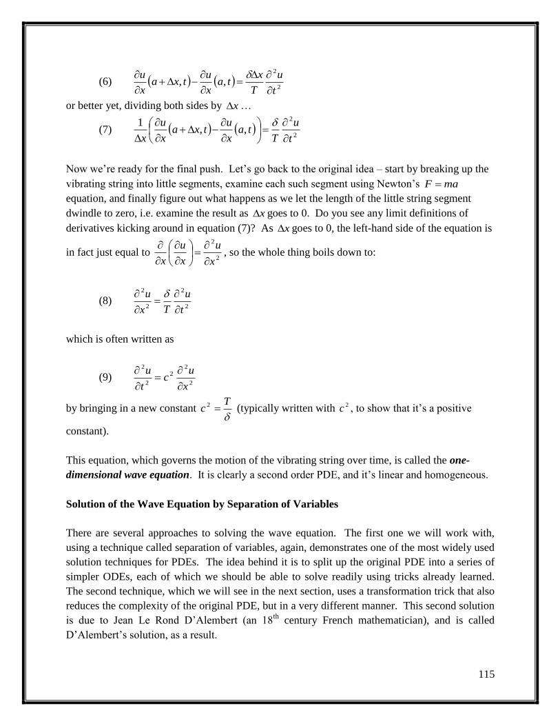
115
(6) 2
2
,,t
u
T
xta
x
utxa
x
u
or better yet, dividing both sides by x …
(7) 2
2
,,1
t
u
Tta
x
utxa
x
u
x
Now we‟re ready for the final push. Let‟s go back to the original idea – start by breaking up the
vibrating string into little segments, examine each such segment using Newton‟s maF
equation, and finally figure out what happens as we let the length of the little string segment
dwindle to zero, i.e. examine the result as x goes to 0. Do you see any limit definitions of
derivatives kicking around in equation (7)? As x goes to 0, the left-hand side of the equation is
in fact just equal to 2
2
x
u
x
u
x
, so the whole thing boils down to:
(8) 2
2
2
2
t
u
Tx
u
which is often written as
(9) 2
22
2
2
x
uc
t
u
by bringing in a new constant
Tc 2 (typically written with 2c , to show that it‟s a positive
constant).
This equation, which governs the motion of the vibrating string over time, is called the one-
dimensional wave equation. It is clearly a second order PDE, and it‟s linear and homogeneous.
Solution of the Wave Equation by Separation of Variables
There are several approaches to solving the wave equation. The first one we will work with,
using a technique called separation of variables, again, demonstrates one of the most widely used
solution techniques for PDEs. The idea behind it is to split up the original PDE into a series of
simpler ODEs, each of which we should be able to solve readily using tricks already learned.
The second technique, which we will see in the next section, uses a transformation trick that also
reduces the complexity of the original PDE, but in a very different manner. This second solution
is due to Jean Le Rond D‟Alembert (an 18th
century French mathematician), and is called
D‟Alembert‟s solution, as a result.
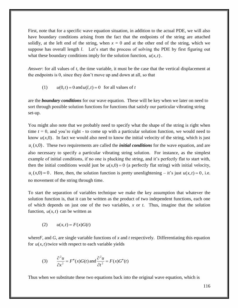
116
First, note that for a specific wave equation situation, in addition to the actual PDE, we will also
have boundary conditions arising from the fact that the endpoints of the string are attached
solidly, at the left end of the string, when x = 0 and at the other end of the string, which we
suppose has overall length l. Let‟s start the process of solving the PDE by first figuring out
what these boundary conditions imply for the solution function, ),( txu .
Answer: for all values of t, the time variable, it must be the case that the vertical displacement at
the endpoints is 0, since they don‟t move up and down at all, so that
(1) 0),0( tu and 0),( tlu for all values of t
are the boundary conditions for our wave equation. These will be key when we later on need to
sort through possible solution functions for functions that satisfy our particular vibrating string
set-up.
You might also note that we probably need to specify what the shape of the string is right when
time t = 0, and you‟re right - to come up with a particular solution function, we would need to
know )0,(xu . In fact we would also need to know the initial velocity of the string, which is just
)0,(xut . These two requirements are called the initial conditions for the wave equation, and are
also necessary to specify a particular vibrating string solution. For instance, as the simplest
example of initial conditions, if no one is plucking the string, and it‟s perfectly flat to start with,
then the initial conditions would just be 0)0,( xu (a perfectly flat string) with initial velocity,
0)0,( xut . Here, then, the solution function is pretty unenlightening – it‟s just 0),( txu , i.e.
no movement of the string through time.
To start the separation of variables technique we make the key assumption that whatever the
solution function is, that it can be written as the product of two independent functions, each one
of which depends on just one of the two variables, x or t. Thus, imagine that the solution
function, ),( txu can be written as
(2) )()(),( tGxFtxu
whereF, and G, are single variable functions of x and t respectively. Differentiating this equation
for ),( txu twice with respect to each variable yields
(3) )()(2
2
tGxFx
u
and )()(
2
2
tGxFt
u
Thus when we substitute these two equations back into the original wave equation, which is

117
(4) 2
22
2
2
x
uc
t
u
then we get
(5) )()()()( 2
2
22
2
2
tGxFcx
uctGxF
t
u
Here‟s where our separation of variables assumption pays off, because now if we separate the
equation above so that the terms involving F and its second derivative are on one side, and
likewise the terms involving G and its derivative are on the other, then we get
(6) )(
)(
)(
)(2 xF
xF
tGc
tG
Now we have an equality where the left-hand side just depends on the variable t, and the right-
hand side just depends on x. Here comes the critical observation - how can two functions, one
just depending on t, and one just on x, be equal for all possible values of t and x? The answer is
that they must each be constant, for otherwise the equality could not possibly hold for all
possible combinations of t and x. Aha! Thus we have
(7) kxF
xF
tGc
tG
)(
)(
)(
)(2
wherek is a constant. First let‟s examine the possible cases for k.
Case One: k = 0
Suppose k equals 0. Then the equations in (7) can be rewritten as
(8) 0)(0)( 2 tGctG and 0)(0)( xFxF
yielding with very little effort two solution functions for F and G:
(9) battG )( and rpxxF )(
wherea,b, p and r, are constants (note how easy it is to solve such simple ODEs versus trying to
deal with two variables at once, hence the power of the separation of variables approach).
Putting these back together to form )()(),( tGxFtxu , then the next thing we need to do is to
note what the boundary conditions from equation (1) force upon us, namely that

118
(10) 0)()0(),0( tGFtu and 0)()(),( tGlFtlu for all values of t
Unless 0)( tG (which would then mean that 0),( txu , giving us the very dull solution
equivalent to a flat, unplucked string) then this implies that
(11) 0)()0( lFF .
But how can a linear function have two roots? Only by being identically equal to 0, thus it must
be the case that 0)( xF . Sigh, then we still get that 0),( txu , and we end up with the dull
solution again, the only possible solution if we start with k = 0.
So, let‟s see what happens if…
Case Two: k > 0
So now if k is positive, then from equation (7) we again start with
(12) )()( 2 tGkctG and
(13) )()( xkFxF
Try to solve these two ordinary differential equations. You are looking for functions whose
second derivatives give back the original function, multiplied by a positive constant. Possible
candidate solutions to consider include the exponential and sine and cosine functions. Of course,
the sine and cosine functions don‟t work here, as their second derivatives are negative the
original function, so we are left with the exponential functions.
Let‟s take a look at (13) more closely first, as we already know that the boundary conditions
imply conditions specifically for )(xF , i.e. the conditions in (11). Solutions for )(xF include
anything of the form
(14) xAexF )(
where k2 and A is a constant. Since could be positive or negative, and since solutions to
(13) can be added together to form more solutions (note (13) is an example of a second order
linear homogeneous ODE, so that the superposition principle holds), then the general solution for
(13) is

119
(14) xx BeAexF )(
where now A and B are constants and k . Knowing that 0)()0( lFF , then
unfortunately the only possible values of A and B that work are 0 BA , i.e. that 0)( xF .
Thus, once again we end up with 0)(0)()(),( tGtGxFtxu , i.e. the dull solution once
more. Now we place all of our hope on the third and final possibility for k, namely…
Case Three: k < 0
So now we go back to equations (12) and (13) again, but now working with k as a negative
constant. So, again we have
(12) )()( 2 tGkctG
and
(13) )()( xkFxF
Exponential functions won‟t satisfy these two ODEs, but now the sine and cosine functions will.
The general solution function for (13) is now
(15) )sin()cos()( xBxAxF
where again A and B are constants and now we have k2 . Again, we consider the boundary
conditions that specified that 0)()0( lFF . Substituting in 0 for x in (15) leads to
(16) 0)0sin()0cos()0( ABAF
so that )sin()( xBxF . Next, consider 0)sin()( lBlF . We can assume that B isn‟t
equal to 0, otherwise 0)( xF which would mean that 0)(0)()(),( tGtGxFtxu , again,
the trivial unplucked string solution. With 0B , then it must be the case that 0)sin( l in
order to have 0)sin( lB . The only way that this can happen is for l to be a multiple of .
This means that
(17) nl orl
n (where n is an integer)
This means that there is an infinite set of solutions to consider (letting the constant B be equal to
1 for now), one for each possible integer n.
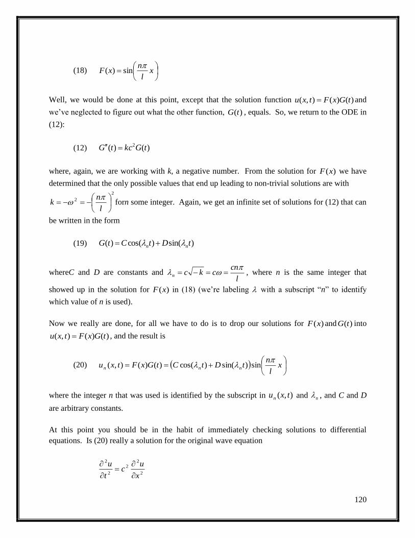
120
(18)
x
l
nxF
sin)(
Well, we would be done at this point, except that the solution function )()(),( tGxFtxu and
we‟ve neglected to figure out what the other function, )(tG , equals. So, we return to the ODE in
(12):
(12) )()( 2 tGkctG
where, again, we are working with k, a negative number. From the solution for )(xF we have
determined that the only possible values that end up leading to non-trivial solutions are with 2
2
l
nk
forn some integer. Again, we get an infinite set of solutions for (12) that can
be written in the form
(19) )sin()cos()( tDtCtG nn
whereC and D are constants and l
cnckcn
, where n is the same integer that
showed up in the solution for )(xF in (18) (we‟re labeling with a subscript “n” to identify
which value of n is used).
Now we really are done, for all we have to do is to drop our solutions for )(xF and )(tG into
)()(),( tGxFtxu , and the result is
(20)
x
l
ntDtCtGxFtxu nnn
sin)sin()cos()()(),(
where the integer n that was used is identified by the subscript in ),( txun and n , and C and D
are arbitrary constants.
At this point you should be in the habit of immediately checking solutions to differential
equations. Is (20) really a solution for the original wave equation
2
22
2
2
x
uc
t
u

121
and does it actually satisfy the boundary conditions 0),0( tu and 0),( tlu for all values of t
The solution given in the last section really does satisfy the one-dimensional wave equation. To
think about what the solutions look like, you could graph a particular solution function for
varying values of time, t, and then examine how the string vibrates over time for solution
functions with different values of n and constants C and D. However, as the functions involved
are fairly simple, it‟s possible to make sense of the solution ),( txun functions with just a little
more effort.
For instance, over time, we can see that the )sin()cos()( tDtCtG nn part of the function
is periodic with period equal to n
2. This means that it has a frequency equal to
2
n cycles per
unit time. In music one cycle per second is referred to as one hertz. Middle C on a piano is
typically 263 hertz (i.e. when someone presses the middle C key, a piano string is struck that
vibrates predominantly at 263 cycles per second), and the A above middle C is 440 hertz. The
solution function when n is chosen to equal 1 is called the fundamental mode (for a particular
length string under a specific tension). The other normal modes are represented by different
values of n. For instance one gets the 2nd
and 3rd
normal modes when n is selected to equal 2 and
3, respectively. The fundamental mode, when n equals 1 represents the simplest possible
oscillation pattern of the string, when the whole string swings back and forth in one wide swing.
In this fundamental mode the widest vibration displacement occurs in the center of the string (see
the figures below).
Thus suppose a string of length l, and string mass per unit length , is tightened so that the
values of T, the string tension, along the other constants make the value of
l
T
21 equal to
440. Then if the string is made to vibrate by striking or plucking it, then its fundamental (lowest)
tone would be the A above middle C.
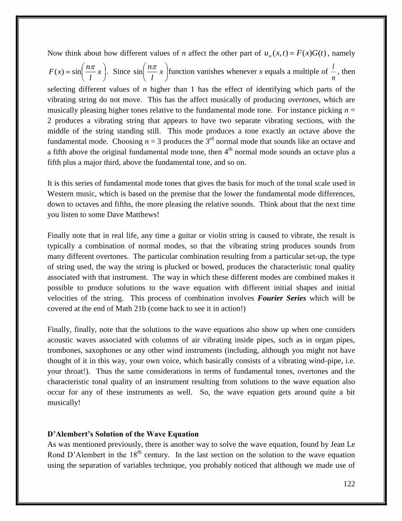
122
Now think about how different values of n affect the other part of )()(),( tGxFtxun , namely
x
l
nxF
sin)( . Since
x
l
nsin function vanishes whenever x equals a multiple of
n
l, then
selecting different values of n higher than 1 has the effect of identifying which parts of the
vibrating string do not move. This has the affect musically of producing overtones, which are
musically pleasing higher tones relative to the fundamental mode tone. For instance picking n =
2 produces a vibrating string that appears to have two separate vibrating sections, with the
middle of the string standing still. This mode produces a tone exactly an octave above the
fundamental mode. Choosing n = 3 produces the 3rd
normal mode that sounds like an octave and
a fifth above the original fundamental mode tone, then 4th
normal mode sounds an octave plus a
fifth plus a major third, above the fundamental tone, and so on.
It is this series of fundamental mode tones that gives the basis for much of the tonal scale used in
Western music, which is based on the premise that the lower the fundamental mode differences,
down to octaves and fifths, the more pleasing the relative sounds. Think about that the next time
you listen to some Dave Matthews!
Finally note that in real life, any time a guitar or violin string is caused to vibrate, the result is
typically a combination of normal modes, so that the vibrating string produces sounds from
many different overtones. The particular combination resulting from a particular set-up, the type
of string used, the way the string is plucked or bowed, produces the characteristic tonal quality
associated with that instrument. The way in which these different modes are combined makes it
possible to produce solutions to the wave equation with different initial shapes and initial
velocities of the string. This process of combination involves Fourier Series which will be
covered at the end of Math 21b (come back to see it in action!)
Finally, finally, note that the solutions to the wave equations also show up when one considers
acoustic waves associated with columns of air vibrating inside pipes, such as in organ pipes,
trombones, saxophones or any other wind instruments (including, although you might not have
thought of it in this way, your own voice, which basically consists of a vibrating wind-pipe, i.e.
your throat!). Thus the same considerations in terms of fundamental tones, overtones and the
characteristic tonal quality of an instrument resulting from solutions to the wave equation also
occur for any of these instruments as well. So, the wave equation gets around quite a bit
musically!
D’Alembert’s Solution of the Wave Equation
As was mentioned previously, there is another way to solve the wave equation, found by Jean Le
Rond D‟Alembert in the 18th
century. In the last section on the solution to the wave equation
using the separation of variables technique, you probably noticed that although we made use of

123
the boundary conditions in finding the solutions to the PDE, we glossed over the issue of the
initial conditions, until the very end when we claimed that one could make use of something
called Fourier Series to build up combinations of solutions. If you recall, being given specific
initial conditions meant being given both the shape of the string at time t = 0, i.e. the function
)()0,( xfxu , as well as the initial velocity, )()0,( xgxut (note that these two initial condition
functions are functions of x alone, as t is set equal to 0). In the separation of variables solution,
we ended up with an infinite set, or family, of solutions, ),( txun that we said could be combined
in such a way as to satisfy any reasonable initial conditions.
In using D‟Alembert‟s approach to solving the same wave equation, we don‟t need to use Fourier
series to build up the solution from the initial conditions. Instead, we are able to explicitly
construct solutions to the wave equation for any (reasonable) given initial condition functions
)()0,( xfxu and )()0,( xgxut .
The technique involves changing the original PDE into one that can be solved by a series of two
simple single variable integrations by using a special transformation of variables. Suppose that
instead of thinking of the original PDE
(1) 2
22
2
2
x
uc
t
u
in terms of the variables x, and t, we rewrite it to reflect two new variables
(2) ctxv and ctxz
This then means that u, originally a function of x, and t, now becomes a function of v and z,
instead. How does this work? Note that we can solve for x and t in (2), so that
(3) zvx 2
1and zv
ct
2
1
Now using the chain rule for multivariable functions, you know that
(4) z
uc
v
uc
t
z
z
u
t
v
v
u
t
u
since ct
v
and c
t
z
, and that similarly
(5) z
u
v
u
x
z
z
u
x
v
v
u
x
u
since 1
x
v and 1
x
z. Working up to second derivatives, another, more involved application
of the chain rule yields that

124
(6)
t
v
zv
u
t
z
z
uc
t
z
vz
u
t
v
v
uc
z
uc
v
uc
tt
u 2
2
22
2
2
2
2
2
22
2
22
2
2
22
2
2
22 2
z
u
vz
u
v
uc
zv
u
z
uc
vz
u
v
uc
Another almost identical computation using the chain rule results in the fact that
(7)
x
v
zv
u
x
z
z
u
x
z
vz
u
x
v
v
u
z
u
v
u
xx
u 2
2
22
2
2
2
2
2
22
2
2
2z
u
vz
u
v
u
Now we revisit the original wave equation
(8) 2
22
2
2
x
uc
t
u
and substitute in what we have calculated for 2
2
t
u
and
2
2
x
u
in terms of
2
2
v
u
,
2
2
z
u
and
vz
u
2
.
Doing this gives the following equation, ripe with cancellations:
(9)
2
22
2
22
2
22
2
22
2
22
2
2
22z
u
vz
u
v
uc
x
uc
z
u
vz
u
v
uc
t
u
Dividing by c2and canceling the terms involving
2
2
v
u
and
2
2
z
u
reduces this series of equations
to
(10) vz
u
vz
u
22
22
which means that

125
(11) 02
vz
u
So what, you might well ask, after all, we still have a second order PDE, and there are still
several variables involved. But wait, think about what (11) implies. Picture (11) as it gives you
information about the partial derivative of a partial derivative:
(12) 0
v
u
z
In this form, this implies that v
u
considered as a function of z and v is a constant in terms of the
variable z, so that v
u
can only depend on v, i.e.
(13) )(vMv
u
Now, integrating this equation with respect to v yields that
(14) dvvMzvu )(),(
This, as an indefinite integral, results in a constant of integration, which in this case is just
constant from the standpoint of the variable v. Thus, it can be any arbitrary function of z alone,
so that actually
(15) )()()()(),( zNvPzNdvvMzvu
where )(vP is a function of v alone, and )(zN is a function of z alone, as the notation indicates.
Substituting back the original change of variable equations for v and z in (2) yields that
(16) )()(),( ctxNctxPtxu
whereP and N are arbitrary single variable functions. This is called D‟Alembert‟s solution to the
wave equation. Except for the somewhat annoying but easy enough chain rule computations,
this was a pretty straightforward solution technique. The reason it worked so well in this case

126
was the fact that the change of variables used in (2) were carefully selected so as to turn the
original PDE into one in which the variables basically had no interaction, so that the original
second order PDE could be solved by a series of two single variable integrations, which was easy
to do.
Check out that D‟Alembert‟s solution really works. According to this solution, you can pick any
functions for P and N such as2)( vvP and 2)( vvN . Then
(17) 22)()(),( 2222 tcctxxctxctxtxu
Now check that
(18) 2
2
2
2ct
u
and that
(19) 22
2
x
u
so that indeed
(20) 2
22
2
2
x
uc
t
u
and so this is in fact a solution of the original wave equation.
This same transformation trick can be used to solve a fairly wide range of PDEs. For instance
one can solve the equation
(21) 2
22
y
u
yx
u
by using the transformation of variables
(22) xv and yxz
(Try it out! You should get that )()(),( yxNxPyxu with arbitrary functions P and N )

127
Note that in our solution (16) to the wave equation, nothing has been specified about the initial
and boundary conditions yet, and we said we would take care of this time around. So now we
take a look at what these conditions imply for our choices for the two functions P and N.
If we were given an initial function )()0,( xfxu along with initial velocity function
)()0,( xgxut then we can match up these conditions with our solution by simply substituting in
0t into (16) and follow along. We start first with a simplified set-up, where we assume that
we are given the initial displacement function )()0,( xfxu , and that the initial velocity
function )(xg is equal to 0 (i.e. as if someone stretched the string and simply released it without
imparting any extra velocity over the string tension alone).
Now the first initial condition implies that
(23) )()()()0()0()0,( xfxNxPcxNcxPxu
We next figure out what choosing the second initial condition implies. By working with an
initial condition that 0)()0,( xgxut , we see that by using the chain rule again on the
functions P and N
(24) )()()()()0,( ctxNcctxPcctxNctxPt
xu t
(remember that P and N are just single variable functions, so the derivative indicated is just a
simple single variable derivative with respect to their input). Thus in the case where
0)()0,( xgxut , then
(25) 0)()( ctxNcctxPc
Dividing out the constant factor c and substituting in 0t
(26) )()( xNxP
and so )()( xNkxP for some constant k. Combining this with the fact that
)()()( xfxNxP , means that )()(2 xfkxP , so that 2)()( kxfxP and likewise
2)()( kxfxN . Combining these leads to the solution

128
(27) )()(2
1)()(),( ctxfctxfctxNctxPtxu
To make sure that the boundary conditions are met, we need
(28) 0),0( tu and 0),( tlu for all values of t
The first boundary condition implies that
(29) 0)()(2
1),0( ctfctftu
or
(30) )()( ctfctf
so that to meet this condition, then the initial condition function f must be selected to be an odd
function. The second boundary condition that 0),( tlu implies
(31) 0)()(2
1),( ctlfctlftlu
so that )()( ctlfctlf . Next, since we‟ve seen that f has to be an odd function, then
)()( ctlfctlf . Putting this all together this means that
(32) )()( ctlfctlf for all values of t
which means that f must have period 2l, since the inputs vary by that amount. Remember that
this just means the function repeats itself every time 2l is added to the input, the same way that
the sine and cosine functions have period 2 .
What happens if the initial velocity isn‟t equal to 0? Thus suppose 0)()0,( xgxut . Tracing
through the same types of arguments as the above leads to the solution function
(33)
ctx
ctxdssg
cctxfctxftxu )(
2
1)()(
2
1),(
In the next installment of this introduction to PDEs we will turn to the Heat Equation.

129
Heat Equation
For this next PDE, we create a mathematical model of how heat spreads, or diffuses through an
object, such as a metal rod, or a body of water. To do this we take advantage of our knowledge
of vector calculus and the divergence theorem to set up a PDE that models such a situation.
Knowledge of this particular PDE can be used to model situations involving many sorts of
diffusion processes, not just heat. For instance the PDE that we will derive can be used to model
the spread of a drug in an organism, of the diffusion of pollutants in a water supply.
The key to this approach will be the observation that heat tends to flow in the direction of
decreasing temperature. The bigger the difference in temperature, the faster the heat flow, or
heat loss (remember Newton's heating and cooling differential equation). Thus if you leave a hot
drink outside on a freezing cold day, then after ten minutes the drink will be a lot colder than if
you'd kept the drink inside in a warm room - this seems pretty obvious!
If the function ),,,( tzyxu gives the temperature at time t at any point (x, y, z) in an object, then in
mathematical terms the direction of fastest decreasing temperature away from a specific point (x,
y, z), is just the gradient of u (calculated at the point (x, y, z) and a particular time t). Note that
here we are considering the gradient of u as just being with respect to the spatial coordinates x, y
and z, so that we write
(1) kjiz
u
y
u
x
uuugrad
)(
Thus the rate at which heat flows away (or toward) the point is proportional to this gradient, so
that if F is the vector field that gives the velocity of the heat flow, then
(2) ))(( ugradkF
(negative as the flow is in the direction of fastest decreasing temperature).
The constant, k, is called the thermal conductivity of the object, and it determines the rate at
which heat is passed through the material that the object is made of. Some metals, for instance,
conduct heat quite rapidly, and so have high values for k, while other materials act more like
insulators, with a much lower value of k as a result.
Now suppose we know the temperature function, ),,,( tzyxu , for an object, but just at an initial
time, when t = 0, i.e. we just know )0,,,( zyxu . Suppose we also know the thermal conductivity
of the material. What we would like to do is to figure out how the temperature of the object,
130
),,,( tzyxu , changes over time. The goal is to use the observation about the rate of heat flow to
set up a PDE involving the function ),,,( tzyxu (i.e. the Heat Equation), and then solve the PDE
to find ),,,( tzyxu .
Deriving the Heat Equation
To get to a PDE, the easiest route to take is to invoke something called the Divergence Theorem.
As this is a multivariable calculus topic that we haven‟t even gotten to at this point in the
semester, don‟t worry! (It will be covered in the vector calculus section at the end of the course
in Chapter 13 of Stewart). It's such a neat application of the use of the Divergence Theorem,
however, that at this point you should just skip to the end of this short section and take it on faith
that we will get a PDE in this situation (i.e. skip to equation (10) below. Then be sure to come
back and read through this section once you‟ve learned about the divergence theorem.
First notice if E is a region in the body of interest (the metal bar, the pool of water, etc.) then the
amount of heat that leaves E per unit time is simply a surface integral. More exactly, it is the
flux integral over the surface of E of the heat flow vector field, F. Recall that F is the vector
field that gives the velocity of the heat flow - it's the one we wrote down as ukF in the
previous section. Thus the amount of heat leaving E per unit time is just
(1) S
SF d
whereS is the surface of E. But wait, we have the highly convenient divergence theorem that
tells us that
(2) E
dVugraddivkd ))((S
SF
Okay, now what is div(grad(u))? Given that
(3) kjiz
u
y
u
x
uuugrad
)(
thendiv(grad(u)) is just equal to
(4) 2
2
2
2
2
2
))((z
u
y
u
x
uuugraddiv

131
Incidentally, this combination of divergence and gradient is used so often that it's given a name,
the Laplacian. The notation uugraddiv )(( is usually shortened up to simply u2 . So
we could rewrite (2), the heat leaving region E per unit time as
(5) E
dVukd )( 2
S
SF
On the other hand, we can calculate the total amount of heat, H, in the region, E, at a particular
time, t, by computing the triple integral over E:
(6) E
dVtzyxuH ),,,()(
where is the density of the material and the constant is the specific heat of the material (don't
worry about all these extra constants for now - we will lump them all together in one place in the
end). How does this relate to the earlier integral? On one hand (5) gives the rate of heat leaving
E per unit time. This is just the same as t
H
, where H gives the total amount of heat in E.
This means we actually have two ways to calculate the same thing, because we can calculate
t
H
by differentiating equation (6) giving H, i.e.
(7)
E
dVt
u
t
H)(
Now since both (5) and (7) give the rate of heat leaving E per unit time, then these two equations
must equal each other, so…
(8)
EE
dVukdVt
u
t
H)()( 2
For these two integrals to be equal means that their two integrands must equal each other (since
this integral holds over any arbitrary region E in the object being studied), so…
(9) )()( 2ukt
u
or, if we let
kc 2 , and write out the Laplacian, u2 , then this works out simply as
132
(10)
2
2
2
2
2
22
z
u
y
u
x
uc
t
u
This, then, is the PDE that models the diffusion of heat in an object, i.e. the Heat Equation! This
particular version (10) is the three-dimensional heat equation.
Solving the Heat Equation in the one-dimensional case
We simplify our heat diffusion modeling by considering the specific case of heat flowing in a
long thin bar or wire, where the cross-section is very small, and constant, and insulated in such a
way that the heat flow is just along the length of the bar or wire. In this slightly contrived
situation, we can model the heat flow by keeping track of the temperature at any point along the
bar using just one spatial dimension, measuring the position along the bar.
This means that the function, u, that keeps track of the temperature, just depends on x, the
position along the bar, and t, time, and so the heat equation from the previous section becomes
the so-called one-dimensional heat equation:
(1) 2
22
x
uc
t
u
One of the interesting things to note at this point is how similar this PDE appears to the wave
equation PDE. However, the resulting solution functions are remarkably different in nature.
Remember that the solutions to the wave equation had to do with oscillations, dealing with
vibrating strings and all that. Here the solutions to the heat equation deal with temperature flow,
not oscillation, so that means the solution functions will likely look quite different. If you‟re
familiar with the solution to Newton‟s heating and cooling differential equations, then you might
expect to see some type of exponential decay function as part of the solution function.
Before we start to solve this equation, let‟s mention a few more conditions that we will need to
know to nail down a specific solution. If the metal bar that we‟re studying has a specific length,
l, then we need to know the temperatures at the ends of the bars. These temperatures will give us
boundary conditions similar to the ones we worked with for the wave equation. To make life a
bit simpler for us as we solve the heat equation, let‟s start with the case when the ends of the bar,
at 0x and lx both have temperature equal to 0 for all time (you can picture this situation as
a metal bar with the ends stuck against blocks of ice, or some other cooling apparatus keeping
the ends exactly at 0 degrees). Thus we will be working with the same boundary conditions as
before, namely

133
(2) 0),0( tu and 0),( tlu for all values of t
Finally, to pick out a particular solution, we also need to know the initial starting temperature of
the entire bar, namely we need to know the function )0,(xu . Interestingly, that‟s all we would
need for an initial condition this time around (recall that to specify a particular solution in the
wave equation we needed to know two initial conditions, )0,(xu and )0,(xut ).
The nice thing now is that since we have already solved a PDE, then we can try following the
same basic approach as the one we used to solve the last PDE, namely separation of variables.
With any luck, we will end up solving this new PDE. So, remembering back to what we did in
that case, let‟s start by writing
(3) )()(),( tGxFtxu
whereF, and G, are single variable functions. Differentiating this equation for ),( txu with
respect to each variable yields
(4) )()(2
2
tGxFx
u
and )()( tGxF
t
u
When we substitute these two equations back into the original heat equation
(5) 2
22
x
uc
t
u
we get
(6) )()()()( 2
2
22 tGxFc
x
uctGxF
t
u
If we now separate the two functions F and G by dividing through both sides, then we get
(7) )(
)(
)(
)(2 xF
xF
tGc
tG
Just as before, the left-hand side only depends on the variable t, and the right-hand side just
depends on x. As a result, to have these two be equal can only mean one thing, that they are both
equal to the same constant, k:

134
(8) kxF
xF
tGc
tG
)(
)(
)(
)(2
As before, let‟s first take a look at the implications for )(xF as the boundary conditions will
again limit the possible solution functions. From (8) we get that )(xF has to satisfy
(9) 0)()( xkFxF
Just as before, one can consider the various cases with k being positive, zero, or negative. Just as
before, to meet the boundary conditions, it turns out that k must in fact be negative (otherwise
)(xF ends up being identically equal to 0, and we end up with the trivial solution 0),( txu ).
So skipping ahead a bit, let‟s assume we have figured out that k must be negative (you should
check the other two cases just as before to see that what we‟ve just written is true!). To indicate
this, we write, as before, that 2k , so that we now need to look for solutions to
(10) 0)()( 2 xFxF
These solutions are just the same as before, namely the general solution is:
(11) )sin()cos()( xBxAxF
where again A and B are constants and now we have k . Next, let‟s consider the
boundary conditions 0),0( tu and 0),( tlu . These are equivalent to stating that
0)()0( lFF . Substituting in 0 for x in (11) leads to
(12) 0)0sin()0cos()0( ABAF
so that )sin()( xBxF . Next, consider 0)sin()( lBlF . As before, we check that B can‟t
equal 0, otherwise 0)( xF which would then mean that 0)(0)()(),( tGtGxFtxu , the
trivial solution, again. With 0B , then it must be the case that 0)sin( l in order to have
0)sin( lB . Again, the only way that this can happen is for l to be a multiple of . This
means that once again
(13) nl orl
n (where n is an integer)
and so

135
(14)
x
l
nxF
sin)(
wheren is an integer. Next we solve for )(tG , using equation (8) again. So, rewriting (8), we
see that this time
(15) 0)()(2
tGtG n
where l
cnn
, since we had originally written 2k , and we just determined that
l
n during the solution for )(xF . The general solution to this first order differential
equation is just
(16) tnCetG
2
)(
So, now we can put it all together to find out that
(17) tnexl
nCtGxFtxu
2
sin)()(),(
Wheren is an integer, C is an arbitrary constant, and l
cnn
. As is always the case, given a
supposed solution to a differential equation, you should check to see that this indeed is a solution
to the original heat equation, and that it satisfies the two boundary conditions we started with.
The next question is how to get from the general solution to the heat equation
(1) tnexl
nCtxu
2
sin),(
that we found in the last section, to a specific solution for a particular situation. How can one
figure out which values of n and Care needed for a specific problem? The answer lies not in
choosing one such solution function, but more typically it requires setting up an infinite series of
such solutions. Such an infinite series, because of the principle of superposition, will still be a
solution function to the equation, because the original heat equation PDE was linear and
homogeneous. Using the superposition principle, and by summing together various solutions

136
with carefully chosen values of C, then it is possible to create a specific solution function that
will match any (reasonable) given starting temperature function )0,(xu .