Embed Size (px)
Citation preview

Institute of Industrial RelationsInstitute of Industrial Relations Working Paper Series
(University of California, Berkeley)
Year Paper iirwps
Impact of Wal-Mart Growth on Earnings
throughout the Retail Sector in Urban
and Rural Counties
Arindrajit Dube Barry EidlinUniversity of California, Berkeley University of California, Berkeley
Bill LesterUniversity of California, Berkeley
This paper is posted at the eScholarship Repository, University of California.
http://repositories.cdlib.org/iir/iirwps/iirwps-126-05
Copyright c©2005 by the authors.

Impact of Wal-Mart Growth on Earnings
throughout the Retail Sector in Urban
and Rural Counties
Abstract
Using a database of Wal-Mart store openings (from Emek Basker), and thecounty level Quarterly Census of Employment and Wages, we estimate the effectof Wal-Mart on earnings of retail workers during the 1990’s economic expansion(1992-2000). We exploit the pattern of Wal-Mart expansion (expanding outwardfrom Arkansas over time) to predict Wal-Mart store openings, allowing us tocontrol for endogeneity using both instrumental variable and control functionapproaches. We find that in urban counties, a Wal-Mart store opening led to a0.5% to 0.8% reduction in average earnings of workers in the general merchandisesector, and a 0.8% to 0.9% reduction in average earnings of workers in thegrocery sector. This translated into a combined 1.3% reduction in total earnings(wage bill) of workers in these sectors. Endogeneity causes the OLS estimatesto be biased downwards in magnitude, primarily from an omitted variables bias.No earnings impact was found for rest of the retail sectors or for restaurants(the latter being an auxiliary test of our identification strategy). In contrast, innon-MSA (i.e., rural) counties, a Wal-Mart store opening was associated with anincrease in earnings of general merchandise workers, and a decrease in earningsof grocery workers, but no significant change in the wage bill. We estimate thatin 2000, total earnings of retail workers nationwide was reduced by $4.7 billiondue to Wal-Mart’s presence.

1
Impact of Wal-Mart Growth on Earnings throughout the Retail Sector
in Urban and Rural Counties
Arindrajit Dube Barry Eidlin Bill Lester
October 2005*
Abstract: Using a database of Wal-Mart store openings (from Emek Basker), and the county level Quarterly Census of Employment and Wages, we estimate the effect of Wal-Mart on earnings of retail workers during the 1990’s economic expansion (1992-2000). We exploit the pattern of Wal-Mart expansion (expanding outward from Arkansas over time) to predict Wal-Mart store openings, allowing us to control for endogeneity using both instrumental variable and control function approaches. We find that in urban counties, a Wal-Mart store opening led to a 0.5% to 0.8% reduction in average earnings of workers in the general merchandise sector, and a 0.8% to 0.9% reduction in average earnings of workers in the grocery sector. This translated into a combined 1.3% reduction in total earnings (wage bill) of workers in these sectors. Endogeneity causes the OLS estimates to be biased downwards in magnitude, primarily from an omitted variables bias. No earnings impact was found for rest of the retail sectors or for restaurants (the latter being an auxiliary test of our identification strategy). In contrast, in non-MSA (i.e., rural) counties, a Wal-Mart store opening was associated with an increase in earnings of general merchandise workers, and a decrease in earnings of grocery workers, but no significant change in the wage bill. We estimate that in 2000, total earnings of retail workers nationwide were reduced by $4.7 billion due to Wal-Mart’s presence. Arindrajit Dube is an economist with the UC Berkeley Institute of Industrial Relations; Barry Eidlin is a PhD student in Sociology at UC Berkeley; Bill Lester is a PhD student in City and Regional Planning at UC Berkeley. *An earlier version of the paper was presented at the American Sociological Association annual conference in August 2005. JEL Classifications: J31, J38, L81

2
1. Introduction and Literature Review
Since opening its first store in 1962 in Rogers, Arkansas, Wal-Mart has grown to be
the world’s largest company. It reported a net income of $9 billion on net worldwide sales of
over $256 billion for the fiscal year ending January 31, 2004 (Wal-Mart Stores 2004). In
2002, Wal-Mart sales accounted for an astonishing 2.3 percent of U.S. GNP (Sperling 2003).
It is also the world’s largest private employer, with over 1.4 million employees, nearly 1
million of them in the U.S. (Ghemawat, Mark and Bradley 2004). Wal-Mart has a dominating
presence the U.S. retail sector: in 2002; fully 82 percent of U.S. households made at least one
purchase at Wal-Mart (Bianco and Zellner 2003). It is already the largest food retailer in the
nation, as well as the third largest pharmacy (Dube and Jacobs 2004), and continues to expand
at a rapid rate (Upbin 2004) – planning an additional 200-250 new stores in the 2006 fiscal
year.
Wal-Mart has achieved this commanding position thanks in part to its pioneering low-
price/high volume business model (Ghemawat, Mark and Bradley 2004). It has squeezed
competitors and suppliers alike by aggressively implementing supply chain operating
efficiencies (Gill and Abend 1997), increasing productivity in distribution (Johnson 2002),
and using its market power to dictate lower prices to its suppliers (Useem, Schlosser and Kim
2003).
However, there is a growing concern that part of Wal-Mart’s success is underpinned
by a compensation practice that keeps wages low. Studies comparing Wal-Mart to other large
retailers nationally find a sizeable gap in average pay (Dube and Jacobs 2004). Furthermore,
anticipated or actual economic pressure from Wal-Mart has been used as a rationale by
competing retailers to seek wage and benefit cuts—as evidenced by the 2003 contract
negotiations between Southern California grocery chains and their unions (Goldman and

3
Cleeland 2003; Pearlstein 2003). In spite of the popular perception that Wal-Mart lowers
wages, however, there is surprisingly little academic work that systematically investigates the
wage consequences of Wal-Mart entry in a regional labor market.
Understanding the impact of Wal-Mart entry on retail-sector wage levels is
important for a number of reasons. If there is indeed a negative “Wal-Mart effect” on wages
in the retail sector, such a finding could be a contender in explaining deteriorating wages for
lower-end workers over the past several decades. Assessing such an effect is also important
for policy makers and communities attempting to weigh the full costs and benefits of Wal-
Mart entry.
Part of the difficulty in identifying a “Wal-Mart effect” is that Wal-Mart’s rapid
expansion occurred simultaneously with ongoing restructuring of the retail industry. This
restructuring is characterized by several trends including: (1) increased consolidation of
retailers into large national chains, (2) the weakening of unions, (3) the introduction of new
technology for inventory control and marketing, and (4) the restructuring of labor processes
including “deskilling” and “reskilling” of jobs. (Davis et al. 2005; Belman and Voos 2004).
The degree to which Wal-Mart in particular is responsible for some of these changes is
difficult to ascertain empirically, despite the plethora of anecdotal and case study examples
that document a significant negative impact. At present, the few studies that directly measure
Wal-Mart’s influence on employment, wages, and working conditions in the retail sector
produce ambiguous results.
Davis et al. (2005) use a detailed matched employer-employee dataset to examine the
impact of big-box retailers (including Wal-Mart) on human resource (HR) practices in the
food retailing industry. They find that traditional grocery stores, which tend to be
characterized by greater use of internal labor markets (ILMs), do not qualitatively alter their

4
labor market practices in the face of spatially localized competition from big-box retailers that
sell food (e.g. a Wal-Mart supercenter). They do find that firms with stronger ILMs are more
likely than non-ILM establishments to go out of business when faced with increased
competition from mass merchandisers. However, this study does not measure the net
employment or wage change after big-box entry; moreover, the authors are not able to control
for possible endogeneity in big-box location decisions.
Basker (2004) examined the impact of Wal-Mart entry on job creation, finding that
“Wal-Mart entry has a small positive effect on retail employment at the county level while
reducing the number of small retail establishments in the county” (p. 19). However, she did
not look at the effect on wages. Moreover, Basker’s identification stragtegy (using store
numbers which reflect the planned sequence of opening to instrument for actual opening) may
not control for endoegeneity bias in her estimates. It is entirely conceivable that most of the
endogeneity in openings operates through the planning stage, as opposed to deviations from
the planned openings. Goetz and Swaminathan (2004) looks at the relationship between Wal-
Mart penetration and overall county-level poverty rates using data from 1987 and 1997. They
find that the growth in Wal-Mart stores between the two years is correlated with a more muted
reduction in poverty rates. They do attempt to control for endogeneity using initial values of
poverty and other “pull factors” to instrument the number of Wal-Marts in 1997. However,
one limitation is that they only consider two years, and are not able to use the timing of store
openings more precisely; moreover, the exogeneity of the determinants of Wal-Mart growth
they use can be debated. Other studies that have examined wages and employment have
arrived at conflicting conclusions.
Many studies are prospective projections based on a direct observation of Wal-Mart’s
lower wages, not empirically observed changes resulting from Wal-Mart’s entry into a

5
market. For example, Randolph (2003) estimates that if Wal-Mart’s market share in the Bay
Area grocery sector were to increase significantly, workers would lose between $353 and 677
million collectively. The few studies that do attempt to empirically estimate the impact of
Wal-Mart entry on county or regional level wage rates focus on a small set of counties in
primarily rural states (Ketchum and Hughes 1997; Hicks and Willburn 1999). For example,
Hicks and Willburn (1999) found a positive wage impact on a set of fourteen counties in West
Virginia. However, their methodology was unable to attribute this wage growth uniquely to
Wal-Mart’s entry, as it was not able to control for endogeneity problems, or even county-
specific factors. Moreover, it is unclear whether the wage impact of Wal-Mart entry in these
rural counties can help us predict impact in more urban areas where most of Wal-Mart’s
current growth is occurring. Because of the methodological shortcomings of previous studies,
it remains to be seen whether there is a general “Wal-Mart effect” on retail sector wage levels
as a whole, based on nationwide data. Since the time of writing this paper, we became aware
of a similar effort by Neumark, Zhang and Ciccarella (2005). They use a similar
identification strategy to estimate the effect of Wal-Mart on labor market outcomes, and the
work was done concurrently to our own (between 2004 and 2005).
This paper estimates the direct impact of Wal-Mart’s expansion on retail sector
earnings in local labor markets. We say direct, as Wal-Mart may also have demonstrative or
standard-setting effects as a dominant player in the American economy—both within the retail
sector and outside. However, such effects are beyond the scope of this paper. Using a
database of Wal-Mart store openings between 1985 and 2001, we identify Wal-Mart’s effect
on earnings of various segments of retail workers. We specifically consider heterogeneous
impact in rural and urban markets. We exploit the pattern of Wal-Mart expansion (expanding
outward from Arkansas over time) to instrument for Wal-Mart store openings. This allows us

6
to control for endogeneity of Wal-Mart entry that might contaminate estimates of Wal-Mart
on earnings. Besides controlling for unobserved factors using an instrumental variables
method, we also test for selection of Wal-Mart into counties where the effect on earnings is
greater (or less) using a control function approach. Finally, we quantify the changes in
aggregate retail workers’ earnings (as opposed to per-worker income) resulting from Wal-
Mart entry.
Our key findings are as follows:
1. In urban counties – i.e., those part of Metropolitan Statistical Areas (MSAs), a
Wal-Mart store opening was associated with:
a. A 0.5%-0.8% reduction in the average earnings of workers in the
general merchandise sector that includes Wal-Mart stores, and a 0.8%-
0.9% reduction in the grocery sector.
b. A 1.3% reduction in total earnings of workers (or wage bill) in general
merchandise and grocery combined.
c. No impact on workers in other retail subsectors or those working in
restaurants; we take this result to be an auxiliary test of our
identification strategy, as we would not expect to see a direct effect of
Wal-Mart growth on restaurant workers.
2. The pattern was different in non-MSA (i.e., rural) counties. A Wal-Mart store
opening was associated with:
a. An increase in the average earnings of general merchandise workers,
and a decrease for grocery workers.
b. No significant change in the wage bill in affected sectors.
c. No impact on other retail sectors or restaurants.

7
3. The majority of Wal-Marts (and an even greater share of new Wal-Mart stores)
is in MSA counties, which employ 85% of general merchandise workers
nationwide. This implies a sizeable wage penalty for the chain’s presence. We
estimate that in 2000, the total earnings of retail workers nationwide was
reduced by $4.7 billion due to Wal-Mart’s presence.
This paper is structured as follows. Section two discusses some theoretical issues to
help interpret possible empirical findings. Section three describes our data sources and
presents our identification strategy. Section four reports both descriptive statistics, and our
key empirical results, as well as results from a variety of specification and robustness tests.
Finally, section five concludes by reviewing the implications of our findings.
2. Theoretical Framework
Interpretations of any possible wage effects of Wal-Mart expansion depend on theories
of wage determination. Moreover, looking at how the diffusion of a particular company
affects wages is atypical in labor economics, and merits a discussion of what might underlie
such an empirical finding.
In the case of a manufacturing company (or one producing goods or services that are
regional exports), the opening of a plant usually reflects the increased profitability for a
certain company in locating production in that area. As a result, employment of workers in
that region by that firm likely represents increased demand for certain types of workers. This
gross job creation then represents net job creation as well. Moreover, it might increase wages
of workers through increased region or industry-level labor demand. If one finds that,
contrary to expectations, a store opening reduces average earnings for workers in a certain
industry, this would imply that perhaps this company was hiring lower-skilled workers (or

8
paying lower labor market rents) as compared to workers already employed in that sector in
that region. However, we would be surprised to find that a store opening reduces total
earnings or the wage bill of workers in that industry, especially if production of that good in
that region was a small fraction of national or global-level output.
However, the economics of the retail labor market are quite different. A new retail
establishment is likely to primarily displace as opposed to create new demand. When Wal-
Mart opens a store, it is unlikely to increase spending by consumers in that region broadly
understood. The key factor in Wal-Mart opening a store in an area is because it can attract
local customers away from existing retailers, probably due to its lower prices. To be sure, it
shifts the composition of sales between narrowly defined areas by attracting consumers from
five, ten or twenty miles away. For instance, sales in the five block radius of a new Wal-Mart
store will most certainly increase. However, county-level sales are unlikely to change much
from a store opening in a given county. Therefore, the key question is whose market share is
Wal-Mart reducing when it sets up shop? Are these companies paying relatively higher
wages and benefits to their workers? If so, then a Wal-Mart expansion might very well
displace better paying jobs with lower paying ones.
The interpretation of “better” or “worse” jobs is not immediate in competitive theories
of the labor market. However, theories incorporating labor market rents allow for a more
realistic evaluation of job quality. There is now a substantial literature that points to the
empirical importance of firm as well as individual-level characteristics in determining the
wage structure (Krueger and Summers 1997). Recent studies incorporating matched
employer-employee data suggest that about half of the variation in wages can be explained by
firm-level characteristics (Abowd et. al 2003). Moreover, there are geographical differences
in the incidence of such high-wage and low-wage firms. For instance, Andersson et al. show
9
that non-urban counties are much more likely to have low-wage firms–i.e., firms that pay
lower wages to similar workers (Andersson, Holzer and Lane 2003). This is important as we
consider the impact of Wal-Mart entry into a regional labor market; if rent-shifting is an
important factor, and Wal-Mart workers earn lower rents, then we might expect Wal-Mart to
have more pronounced effects in urban areas.
Besides affecting wages in general merchandising, where Wal-Mart competes directly,
through a composition effect, Wal-Mart might also have an effect on competing industry
segments. This is particularly true with grocery. Wal-Mart supercenters have drawn away
business from traditional format supermarkets in many areas. Supermarkets typically pay
higher wages, and have higher rates of unionization than other retail segments. In 2005,
according to the Current Population Survey, the unionization rate in supermarkets was 21%,
as opposed to 5% in general merchandising (discount stores and department stores) and 6% in
retail overall. Similarly, the union wage premium for supermarkets was 27%, as opposed to
6% and 8% for general merchandising and all retail, respectively. Therefore, competition
from the non-union Wal-Mart chain might particularly be of relevance for earnings if Wal-
Mart displaces unionized supermarket jobs.
Beyond rent-shifting, Wal-Mart might also reduce earnings through employing a
different “skill mix” of workers. If the chain has a particular advantage in employing workers
with lower skill levels, a reduced average (or total) earnings in the general merchandise sector
might reflect a changed composition of the workforce. Reduced average (but not total)
earnings in competing segments is harder to explain using purely competitive stories. For
instance, if such reductions only reflect skill-switching, it begs the question of why increased
product market competition would lead competitors to change the skill mix of workers.
However, more complicated stories involving complementarities between skill and service

10
quality could potentially rationalize such a finding with fully competitive model. For
instance, if low-price competition from Wal-Mart leads to supermarkets reducing both
compensation and service quality (which in turn depends on compensation), then one may still
be able to give a competitive interpretation of a change in earnings.
All in all, a finding of a more pronounced average wage reduction in (higher rent)
urban areas, along with a reduction in wages in competing segments, would in our view
suggest that at least some of the reduction in earnings due to Wal-Mart entry reflects a
reduction in worker rents.
3. Data and Empirical Methodology
3.1. Data Sources
Our primary unit of analysis for examining local labor markets is the county. For
information on employment and annual earnings, we use the Quarterly Census of
Employment and Wages (QCEW) dataset compiled by the U.S. Bureau of Labor Statistics.
The QCEW dataset is based on information filed by all private employers with State
unemployment insurance agencies. Data on total employment (headcount) and the total
earnings (wage bill) is reported at the 3-digit SIC level (Standard Industrial Classifications).
We construct the average earnings for workers in a given industry by dividing the wage bill
by the headcount measure for that industry. Given our data, that we are not able to distinguish
between a reduction in average annual earnings that is due to lower hours of work from one
that is due to lower hourly wages. The QCEW data was supplemented by (1) population
estimates for each county from the 2000 and 1990 Census; and (2) the spherical distance
between the geographic center of a county to Benton county, Arkansas, using GIS software
(ArcView) and Census shape files.

11
We restrict our analysis to the 1992-2000 period for several reasons. First of all, this is
the period when Wal-Mart really expanded outside the South, and into major metropolitan
areas. If the Wal-Mart effect is heterogeneous, then using older periods may be of less
interest in understanding how Wal-Mart growth is affecting wages in places it is growing
today. Second, focusing on the period of economic expansion reduces possible confounding
effects of comparing years when the economy was growing versus shrinking.1
To track Wal-Mart entry over time by county, we use a database of Wal-Mart
locations compiled by Emek Basker.2 (For more information about this dataset, see Basker,
2004.) Basker used three main sources for this information, namely: 1) the Rand-McNally
Business Atlas, and 2) Chain Store Guide, and 3) annual reports filed by Wal-Mart with the
Securities and Exchange Commission (SEC). Our study uses data from 1988 to 2001 period,
which come from (1) and (2). The dataset documents Wal-Mart store openings by year since
its founding in 1962 up to 2001, disaggregated by state, county, town, and zip code. We
aggregated this data to the county level to match the QCEW.3 The dataset includes Wal-Mart
discount stores, supercenters and neighborhood markets, but not Sam’s Club stores.
The final dataset contains county-year level observations, with data on employment,
total earnings and average earnings for the following industries: (1) general merchandise, (2)
grocery, (3) rest of retail, (4) restaurants, and (5) the full labor force. Other variables include
2 The Wal-Mart database was made available to us to look at Wal-Mart’s impact on wages, employment, taxes, or public assistance. Her generosity in providing this dataset is graciously acknowledged. 3 Basker argues that the Chain Store Guide might be reporting the presence of a store when it was merely planned to be opened. To account for this possibility, we tried offsetting the store openings in this period by a year as a check. This did not substantively change any of our baseline estimation results. The CSG also appears to not have been fully updated in the 1990-1993 period. Basker imputes the store openings between 1990-1993 using an algorithm explained in Appendix A1 in her paper. We also repeated the analysis using only the 1994-2000 period, and again, the baseline results were nearly identical.

12
the total number of Wal-Marts, distance from Benton County, and county population.
Finally, we exclude counties with incomplete data (due to non-disclosure in the case of very
small counties) for each industry4. In other words, for each retail segment, we only use
counties which have full set of disclosed data for that industry. These excluded smaller, rural
counties with little employment in general merchandise or grocery sectors.
3.2. Estimating Impact on Average Earnings 3.2.1 Baseline Specification
Any correlation between Wal-Mart presence and retail sector earnings may be driven
by a number of confounding factors. Most simply, Wal-Mart may enter into low-wage
counties. For instance, Wal-Mart’s presence is greater in the South, and the South has
generally lower overall wages, lower levels of unionization, and typically does not have state-
level minimum wages that exceed the federal standard. Similarly, county-specific unobserved
demographic patterns that limit the supply of low-skilled labor (e.g. a county with a very old
population) may result in higher wages for all retail sector workers. Finally, it may be that
Wal-Mart enters counties that have generally declining wages (or employment), or that Wal-
Mart entry happens at a time when workers’ wages were particularly low.
To control for these factors, we estimate the wage impacts using a number of different
specifications. The first specification is a simple fixed-effect model, which regresses the
natural log of average annual earnings of various types of retail workers (ln(earn)) on the
number of Wal-Marts that year (WM), and county and year dummies. To control for local
4 To avoid identifying individual respondents the QCEW withholds data for industries in counties with very few employers or where a single firm represents more than 80% of the total industry employment. These ‘non-disclosed’ cases are flagged in the data.

13
labor market conditions, we include the log of average earnings for the total workforce in the
county as an added regressor (earnT).
(1) 0 1ln( ) ln( )Tit it it t i itearn earn WM year County eβ β ϕ= + + + Λ ⋅ + Ω ⋅ +
This can be implemented by running a first-difference OLS regression:
(2) 0 1ln( ) ln( )Tit it it t itearn earn WM year eβ β ϕ∆ = + ∆ + ∆ + Λ ⋅ + ∆
A fixed-effect model does not rule out the possibility that Wal-Mart is entering
counties that would otherwise have experienced faster or slower wage growth. Formally, it
may be that ( , ) 0it itCov e WM∆ ≠ , that the change in the number of Wal-Mart stores is
correlated with the residual wage growth in that county. The primary way we address the
endogeneity issue in this paper is by exploiting the spatial pattern of Wal-Mart growth.
“Ground zero” for Wal-Mart was Benton county in Arkansas. Wal-Mart opened its first store
in the town of Rogers, which is part of this county; and its present day headquarters is located
in Bentonville, also in Benton County. Over time, Wal-Mart spread out over the rest of the
country. But it did not do so in a haphazard manner. For instance, it didn’t jump to New
York, then to California, to then back to Tennessee. Rather, the spatial diffusion was much
more concentric: grow in areas near your existing operations before jumping to farther areas.
The only caveat to this rule is that Wal-Mart often left larger cities alone as it expanded
initially, suggesting that the distance/growth relationship should probably be estimated
differently for urban and non-urban areas. The diffusion process over this period can be seen
in Maps 1-3, and Figures 6 and 7, and is discussed in greater detail in section 4.1. The most
likely reason for this growth pattern is that Wal-Mart wanted to make the most out of its local
infrastructure such as distribution networks (Holmes 2005). Holmes argues that these
economies of density can help explain the growth process exhibited by Wal-Mart. An earlier

14
paper by Thomas Graff also documented Wal-Mart’s strategy of locating Supercenters in
places where they already had an existing grocery distribution network (Graff 1998). Graff
contrasts this with Kmart, which seemed to set up its supercenters without taking advantages
of such economies of density. A corollary to this pattern of growth is that, on average, the
farther a county is from Benton, the later it experienced Wal-Mart growth.
The timing of growth allows for an interesting identification strategy. We can use the
distance from Benton county (dist) as an instrument for the change in the number of Wal-Mart
stores in a given county for a given year. Consequently, in the second stage we would only
use the variation in Wal-Mart growth that is related to how far the county is from Benton. To
implement this strategy empirically, we utilize a flexible specification in the first stage by
forming J discrete distance quantiles (or rings) defined by the distance between the
geographic center of a county from Benton, and interact these with year dummies. (In the
baseline specification, J=10.) The predicted number of Wal-Marts (and the change in the
number of Wal-Marts) is then only a function of the distance quantile of the county and the
year. The predicted change in the number of Wal-Marts is used in the second stage to
estimate the impact on earnings. The next two equations formalize this logic:
(3) 0it jt t j tjtWM Year Distη η ε= + ⋅ ⋅ +∑
(4) 0 1ln( ) ln( )Titit it t itearn earn WM year eβ β ϕ∆ = + ∆ + ∆ + Λ ⋅ + ∆
The inclusion of earnT in the second stage may raise questions for some. Indeed, if we
were fully confident of our exclusion restriction, why would we add any additional controls?
There are two reasons why we believe that this is warranted (although as we show below, this
addition is not of empirical importance). We believe that looking at the deviation of retail
sector earnings from average earnings makes the identification strategy more credible. For

15
instance, it might be that in our sample of nine years, there was a secular trend of a shrinking
income gap between the Southern US and rest of the country. This would be a problem when
one looks at a relatively small number of years where regions (not just counties) might have
autocorrelative trends. However, we feel that it is harder to explain away why specifically
certain narrow sectors (where Wal-Mart competes) would be see a decline in relative earnings
that is correlated with the spatial diffusion of Wal-Mart absent a causal effect.
The instrumental variable produces consistent estimates of the average treatment effect
if the following assumptions hold:
(A1) it ije dist⊥ ,
(A2) i itWMϕ ⊥ ∆ .
The first is an exclusion restriction, which requires that the residual retail earnings
growth in year t is stochastically independent of the distance quantile. The second states that
the true effect of Wal-Mart on retail earnings is uncorrelated with Wal-Mart growth—that the
treatment effect is independent of the treatment status. The latter is always satisfied in a
constant coefficient model.
In a random coefficient model, if the treatment effect ( iϕ ) is both heterogeneous and is
not independent of the incidence or extent of treatment (i.e., Wal-Mart penetration), the IV
approach no longer estimates the average treatment effect—for either the entire population or
those experiencing Wal-Mart growth. Rather, it estimates the average treatment effect for a
arbitrary subset of the population – whose treatment status is affected solely by the variation
in the instrument. Under certain assumptions, a control function approach can correct for both
confoundedness due to omitted variables (correlated with Wal-Mart entry) as well as
selectivity of Wal-Mart entry by treatment effect (see Garen 1986; Heckman and Vytlacil

16
1999; Chay and Greenstone 2005). The control function (CF) can be implemented through a
two-stage process, where the first stage (as before) regresses the number of Wal-Marts on a
function of time and distance. In the second stage, we include the treatment variable, as well
as both the residuals from the first stage and the residuals interacted with the treatment
variable as added regressors.
(5) 0it jt t j itjtWM Year Distη η ε= + ⋅ ⋅ +∑
(6) 1it it itres ε ε −= −
(7) ( )0 1 1 2ln( ) ln( )Tit itit it it it t itearn earn WM res res WM year eβ β ϕ δ δ∆ = + ∆ + ∆ + ∆ + ∆ ⋅ + Λ ⋅ + ∆
Here, the fittedϕ is a consistent estimator of the average treatment effect. The
coefficient 1δ measures the importance of omitted variable bias—how much such omitted
variables may contaminate the OLS estimate. The coefficient 2δ measures the selection
effect—the extent to which Wal-Mart entry may be correlated with the (heterogeneous)
treatment effect.
We estimate all the models for the general merchandise sector (SIC 53), which
includes discount stores and department stores such as Wal-Mart, Kmart, Target, Costco, and
Sears. In addition, we estimate the models for grocery (SIC 54). We also estimate these two
sectors together. We then estimate the models for other retail sectors together (except for
restaurants (SIC 58)). As an added check, we perform the same regressions for restaurants as
well. Since it is unlikely that Wal-Mart would affect relative earnings of restaurant workers
(especially in larger labor markets), we take this to be an auxiliary test of our identification
strategy. Finally, all of the above regressions are estimated using weights corresponding to
the county population levels from 2000 census; this technique implies that the treatment effect

17
to be representative of the population (and hence typically the workforce) as a whole. Using
employment in the relevant subsectors in the county (such as general merchandise) as the
weight is problematic, since the same variable is used to compute average earnings, a
dependent variable. To verify that our results are not driven by use of the weight, we also
report unweighted baseline specification results.
The effect of an added Wal-Mart on the average earnings of retail subsectors is likely
to be different in metropolitan counties than rural ones, both because MSA counties are denser
and because there may be different wage standards in place. Therefore, we perform separate
first and second stage regressions for counties that are part of Metropolitan Statistical Areas
(MSAs) and those that are not, using the 1998 MSA definitions. The MSA definition is kept
constant to avoid an artificial “growth” in Wal-Mart stores in a MSA as counties may be
added over time.
3.2.2 Alternative First Stage Specifications– Predicting Wal-Mart Openings Using Distance from Arkansas The IV and CF estimates above were based on the “baseline” first stage specification
using ten distance quantiles to predict Wal-Mart growth. As a robustness check, we
investigate the impact of specifying a different number of quantiles. Specifically, we estimate
equations (3) to (7) using anywhere between 4 and 20 such bins to evaluate how sensitive the
estimates are to the width of the bins. Generally, using fewer bins will mean that we lose
statistical power in predicting Wal-Mart growth; however, given a finite sample, increasing
the number of bins will eventually lead the IV estimate to be equal to the OLS one (in the
extreme case where each county is its own bin). Ideally, we would find a substantial range
with a reasonable number of bins that all produce similar point estimates.

18
As a final check on the first stage specification, we also fit a set of parsimonious
specifications, where the number of Wal-Marts in a county is predicted by a combination of a
time variable (2001 minus year), a distance variable (distance of the county’s center from that
of Benton county), the product of time and distance, as well as quadratic terms of these
variables. The three variations of the first stage are as follows:
(8) 0 1 (2001 )it t j itWM Year Distη η ε= + ⋅ − ⋅ +
(9) 0 1 2 3(2001 ) (2001 )it t i t i itWM Year Dist Year Distη η η η ε= + ⋅ − ⋅ + ⋅ − + ⋅ +
(10) ( )2 2
0 ,0 0
(2001 )m nit m n t i it
m n
WM Year Distη η ε= =
= + ⋅ − ⋅ +∑∑
Using these first stage specifications, we estimated the IV and CF formulations (equations (4),
(6), and (7)), for both general merchandise and grocery sectors.
3.2.3 Second Stage Estimation Using Information on Time of Entry
If the Wal-Mart effect occurs with a lag, then the coefficients in the baseline
specification represent the treatment effect averaged over the distribution of tenure for stores
opening in our sample. One concern is that this does not make full use of the information on
the timing of Wal-Mart entry to identify the effect on earnings. For this purpose, we develop
a set of alternative second-stage specifications that estimate the effect on earnings three years
after a store opens. For the purpose of this analysis, we can no longer use the control-function
approach, as our identification assumptions are no longer maintained with the inclusion of
leads and lags. However, the IV specification still identifies the average treatment effect if
conditions (A1) and (A2) hold: that the treatment effect (with any lags in this case) is
independent of Wal-Mart entry, and that the residual retail earnings changes are stochastically
independent of the distance quantile a county is in.

19
To use information on the exact timing of entry, we additionally include a lead
variable and three lag variables. This is done for both the OLS and IV formulations
(11) 3
0 11
ln( ) ln( ) ( )T jit it k it t it
k
earn earn L WM year eβ β ϕ=−
∆ = + ∆ + ∆ + Λ ⋅ + ∆∑
(12) 3
0 11
ln( ) ln( ) ( )T jitit it k t it
k
earn earn L WM year eβ β ϕ=−
∆ = + ∆ + ∆ + Λ ⋅ + ∆∑
Here, the effect of a new Wal-Mart store on average earnings three years after the
store opening is computed as 3
0j
j
ϖ ϕ=
=∑ . The inclusion of the lead variable 1WM −∆
(or 1WM −∆ ) means that we are considering changes in wages from the year prior to Wal-Mart
entry.
To check for sensitivity of our time-trend assumptions, we also fit second-difference
forms of (11) and (12), which allow for county-specific trends.
(13) ( )
( )
3
1 0 11
1
ln( ) ln( ) ln( ) ln( ) ( )T T jit it it it k it
k
t it it
earn earn earn earn L WM
year e e
β β ϕ−=−
−
∆ − ∆ = + ∆ − ∆ + ∆ ∆
+ Λ ⋅ + ∆ − ∆
∑
(14) ( )
3
1 0 11
ln( ) ln( ) ln( ) ln( ) ( )T T jitit it it it k
k
t it
earn earn earn earn L WM
year e
β β ϕ−=−
∆ − ∆ = + ∆ − ∆ + ∆ ∆
+ Λ ⋅ +
∑
Our final specification is an event study type approach, which includes a larger set of
leads and lags to tease out the time path of earnings. The advantage is that one can visually
better assess the impact of store openings on earnings over time. The disadvantage is the
inclusion of leads also limits the number of years we can use (as our Wal-Mart data is only
through 2001). We fit this for the IV formulation.
(15) 3
0 14
ln( ) ln( ) ( )T jitit it k t it
k
earn earn L WM year eβ β ϕ=−
∆ = + ∆ + ∆ + Λ ⋅ + ∆∑

20
3.3 Estimating Impact on Total Earnings (or Wage Bill)
Finally, we examine the impact of an additional Wal-Mart on the total wage bill paid
by firms in the general merchandise and narrow retail sectors. Given Basker’s (2004) finding
of a slight net increase in county retail employment following the opening of a Wal-Mart
store, we estimate the combined effect of Wal-Mart on employment and average wages on
county-level earnings of the relevant retail workers.
Here we estimate the impact of store openings on the combined wage bill of both
general merchandise and grocery subsectors. As before, we estimate the regression in first-
difference form to purge any county fixed effects, and include year dummies. We include the
average earnings and overall employment in the county as added regressors to control for any
county-year specific changes in the wage bill. Equations (16)-(18) estimate the impact on the
wage bill of general merchandise and grocery from an added Wal-Mart store using OLS, IV,
and CF approaches, respectively.
(16) 0 1 2ln( ) ln( ) ln( )T Tit it it it
t it
wagebill earn employment WM
year e
β β β ϕ∆ = + ∆ + ∆ + ∆ +
+ Λ ⋅ + ∆
(17) 0 1 2ln( ) ln( ) ln( )T Titit it it
t it
wagebill earn employment WM
year e
β β β ϕ∆ = + ∆ + ∆ + ∆ +
+ Λ ⋅ + ∆
(18) 0 1 2 1
2
ln( ) ln( ) ln( )T Titit it it it
it it t it
wagebill earn employment WM res
res WM year e
β β β ϕ δ
δ
∆ = + ∆ + ∆ + ∆ +
+ ⋅ ∆ + Λ ⋅ + ∆
4. Findings 4.1 The Nature of Wal-Mart Growth

21
Wal-Mart increased its number of U.S. stores between 1988 and 2000 by almost
150%, from 1,070 to 2,449 (Figure 1). In 1988 Wal-Mart was concentrated in the rural South
and Midwest. By 2000, Wal-Mart had expanded rapidly into the West and Northeast.
Figure 2 reports the distribution of stores by region, showing a heavy concentration of
Wal-Mart stores in the South and also in the Midwest, and rapid growth in the West and
Northeast. While this store distribution is in keeping with the company’s Southern origin it
also reflects a pattern of national expansion.
Wal-Mart’s growth pattern is also represented spatially in Maps 1-3. In 1988, Wal-
Mart was clearly concentrated in the South and the (lower) Midwest, with no stores in the
New England area or west of the Rockies. Six years later, however, Wal-Mart’s store
network had expanded significantly to include several stores in California and many in the
Northeast. By 2000, Wal-Mart’s network is truly national, with stores in every major
metropolitan area. In the 1990’s Wal-Mart grew from a primarily Southern, rural retailer to
become a nationally dominant metropolitan-based (urban and suburban) company. Maps 1-3
demonstrate the basis for our instrumenting strategy. Wal-Mart expanded outward
geographically from its home base in Arkansas over time. Typically, the farther a county was
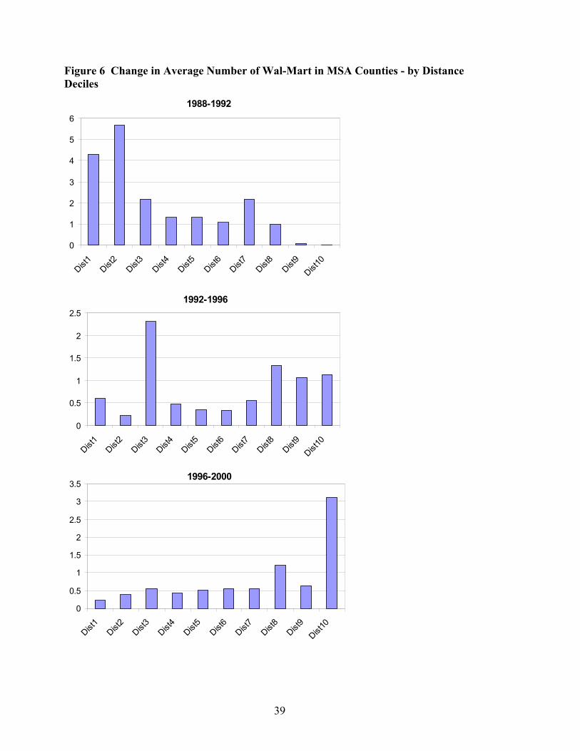
located from Benton county, the later the date of Wal-Mart entry. Figure 6 makes this point
for the 1988 to 2000 period by tabulating Wal-Mart growth for distance deciles for MSA
areas; Figure 7 does the same for non-MSA areas. In both figures, we see that the growth in
early nineties was concentrated in lower deciles. By late nineties, the growth was
concentrated in upper deciles.
While this expansion helped Wal-Mart reach nearly all U.S. consumers it also greatly
expanded the size and geographic scope of Wal-Mart’s workforce. Figure 3 shows that Wal-
Mart went from having at least one store in 823 of 3,064 counties (27%) in 1988, to 1,630 of

22
3,064 counties (53%) in 2000. Wal-Mart’s growth over the more recent period has come
disproportionately from expansions in metropolitan areas. This growth pattern brings Wal-
Mart into close contact with the majority of the nation’s retail workforce. Figure 4 shows the
change in the distribution of employees in counties with at least one Wal-Mart; the 27% of
counties with at least one Wal-Mart in 1988 had 25% of the nation’s retail workforce. By
2000, that number had changed dramatically. The 53% of counties with at least one Wal-Mart
contained 86% of the total retail workforce. In other words, most retail workers in 2000 were
in markets with some exposure to Wal-Mart.
Overall, we find that as Wal-Mart expanded throughout the 1990s, it moved into
larger, more densely populated counties. Between 1988 and 2000, the share of non-MSA
counties with at least one Wal-Mart rose from 25% to 43%. However, the share of MSA
counties with a Wal-Mart presence rose from 33% to 79% over the same period. Retail
workers in urban areas experienced a sharp increase in exposure to Wal-Mart over the
nineties.
4.2 Impact of Wal-Mart Growth on Retail Earnings in MSA Counties
4.2.1 Effect on average earnings
Table 1 presents the own-county impact of Wal-Mart stores on earnings in MSA
counties. We estimate the 3 baseline specifications – OLS, IV and CF – for general
merchandise, grocery, and broad retail. Looking at general merchandise (column 1), we find
that the presence of an additional Wal-Mart corresponds to lower earnings in all three
specifications. The coefficients suggest that an additional Wal-Mart reduces the average
earnings by between 0.4 and 0.8 log points (i.e., by around 0.4% to 0.8%), and these
coefficients are all statistically significant at the 1% level.

23
To put this in perspective, in 2000, the mean general merchandising employment in a
MSA county was 4,100, while the mean earnings was $15,700. If a typical Wal-Mart store
had around 350 workers, a single Wal-Mart store would reduce the average wage earned by
the 4,100 workers by $125 annually (using the IV estimate). If we assume that in the general
merchandise sector, all the reduction in average earnings occurred through a composition
effect (Wal-Mart displacing better paying jobs), we can calculate the implied earnings gap
between workers at Wal-Mart versus other general merchandisers shedding employment due
to Wal-Mart entry. 350 Wal-Mart workers constitute roughly 8.5% of a county’s general
merchandise workforce. So if earnings of the other 91.5% stayed same, but overall earnings
declined by 0.8%, this implies that those losing jobs at other general merchandise retailers
were making around 10% more than Wal-Mart workers. Of course, this is only an
approximation; to the extent Wal-Mart also reduced wages of competitors, the implied gap
would be lower.
As Table 1 shows, the IV estimate is the biggest in magnitude, while the OLS is the
smallest, with the CF estimate is somewhere in between. Looking at the coefficients on the
omitted variable bias and selection bias clarifies the reason for the different estimates. The
omitted variable bias is positive, meaning that unobserved variables are positively correlated
with general merchandise wage and Wal-Mart growth. This pattern explains why the OLS is
biased downwards. However, the selection bias is negative, which suggests that Wal-Mart
tended to come into counties where there would be particularly large wage reduction,
clarifying why the IV to be greater in magnitude that the CF estimate. This is consistent with
an economic model where Wal-Mart finds markets where competitors are paying particularly
high rents to workers most appealing to enter, as these competitors would have a bigger cost

24
disadvantage. Overall, however, the net impact of the omitted variable bias trumps the
selection effect—something that is found throughout the analysis.
Earnings in the grocery sector are also reduced by Wal-Mart presence (column 2). All
three specifications produce negative coefficients that are statistically significant at the 1%
level. However, the gap between the OLS estimate on the one hand (0.1%) and IV and CF
estimates on the other (0.8% and 0.9%, respectively) are substantially larger for this sector
than for general merchandise. It appears that the selection effect, where Wal-Mart comes into
areas where it lowers the wage the most, is not a factor in the case of grocery.
Earnings in grocery and general merchandise together also show a negative Wal-Mart
effect (column 3). We also estimate three other versions of this regression (combined general
merchandise and grocery earnings) to check the impact of various assumptions on our core
results. Column 4 shows the estimates without using population weights. We find that all the
treatment coefficients are negative and significant as before, but the magnitudes are much
larger. For instance, the CF and IV coefficients are now -0.035, as compared to -0.006 and -
0.007 previously. This is not surprising, since the effect of a single store on earnings in a
county with a large population will doubtless be smaller than the effect in a less populous
county. A single store would have a smaller share of the market in less populated county.
Weighting by population puts more weights on larger and denser counties. To get a treatment
effect that is representative of the workforce, it is reasonable to use such population weights;
however, it is reassuring that the finding of earnings reduction is not driven by large cities.
Column 5 reports the estimates that add restaurant wages as an additional control. Comparing
columns 3 and 5, we see that the additional control has no impact on the estimates. Finally,
column 6 repeats the regression, but this time without county-level earnings as a control. IV

25
and CF coefficients are only slightly smaller in magnitude in this specification; for instance,
our CF estimates fall in magnitude from -0.60 to -0.051.
The Wal-Mart effect appears to be concentrated in the retail subsector where the store
competes. For rest of retail, the coefficient on Wal-Mart is not statistically significant in any
of the specifications.
Finally, we find that for restaurant workers (another set of low wage workers), Wal-
Mart has no effect on earnings. This lack of finding an effect in restaurants provides
additional support for our identification strategy: it is unlikely that restaurant wages in urban
areas (with dense labor markets) would be affected by Wal-Mart entry.
4.2.2 Robustness checks for first stage specifications
Our first stage specification was based on distance deciles, allowing for a flexible
pattern of growth of Wal-Mart as one moves further away from Benton county. We perform
sensitivity analysis on the first stage by using alternative numbers of quantiles (between 4 and
20), as well as allowing for more parsimonious specifications that include the year, year times
distance, and higher order terms of these variables).
When we consider alternative number of distance bins, all the alternative first-stage
specifications produce a negative and statistically significant effect of Wal-Mart on earnings
for general merchandise and grocery workers (Table 2). Moreover, we find that with very
small number of bins (6 or less), the estimated coefficients are somewhat larger. However,
for more than 6 bins, the coefficients tend to stabilize, for both IV and CF estimates, and for
both general merchandise and grocery sectors. This gives us confidence that the broad results
of our baseline first-stage specification are not being driven by bin width.

26
When we look at the more parsimonious formulations, using linear or quadratic terms
in time and distance from Benton county, we find that all the estimated earnings effects are
negative and significant at the 1% level. The coefficients for general merchandise (in both IV
and CF formulations) are quite close to the more flexible baseline specification. However, the
grocery earnings coefficients are larger in magnitude. This suggests that imposing too much
structure on the first stage regression predicting Wal-Mart expansion may be problematic.
4.2.3 Time path of Wal-Mart’s effect on wages
In Table 4, we present the estimates from various specifications using lags and leads,
and from alternative specifications of time trends. For general merchandise, the OLS estimate
of the three-year effect is -0.0023 in the first-difference specification, and 0.048 in the second-
difference one. Both estimates are statistically significant and negative. The IV estimates of
the three-year effect range from -0.0087 and -0.0148, again all statistically significant at the
5% level, and larger in magnitude than the corresponding OLS estimates.
For the grocery sector, the findings are analogous. OLS estimates are smaller in
magnitude, ranging between -0.0015 and -0.0023, both being significant at the 10% level. In
contrast, the IV estimates are greater in magnitude, lying between -0.0057 and -0.0128, all
statistically significant at the 5% level. As before, we find that the broader retail sector
earnings are unaffected by Wal-Mart entry. In most specifications, these coefficients are
positive, but have large standard errors and are not close to being statistically significant.
Table 4 also presents the coefficients from the event study type specification using the
instrumental variable method. The time paths are demonstrated visually in Figures 8 to 10,
along with the 95% confidence interval bands around the point estimates. The table and the

27
figures show that the three-year effects for both general merchandise and grocery are negative
and significant, and fall within the range of estimates in other specifications. It is also
visually apparent that the wages fall over the 3 years subsequent to store opening, although
the adjustment seems to be much more rapid in grocery. In contrast, as Figure 8 shows, the
rest of retail earnings coefficients have very large standard errors, and do not point to any
systematic changes following Wal-Mart entry.
Overall, the specification checks in this and the previous section indicate that there is a
substantial and the statistically significant effect of Wal-Mart growth on average earnings of
urban retail workers, and that the effect is concentration in the two subsectors, namely,
general merchandising and grocery.
4.2.4 Effects on retail sector wage bills
The final labor market impact we model is the effect of Wal-Mart entry on the wage
bill (i.e., total earnings by all workers) in retail sectors. This model measures the combined
effect of reduced wages in the general merchandise and grocery subsectors and the net job
growth (or loss) associated with new Wal-Mart stores. Table 5 summarizes the results of
these estimates based on baseline specifications as denoted in equations (16) - (18). We
report the findings using OLS, IV and CF approaches.
All three approaches show substantial and statistically significant reduction in the
wage bill in grocery and general merchandise sectors. The OLS estimate suggests that a Wal-
Mart store opening reduces the combined earnings of general merchandise and grocery
workers in metropolitan counties by around 0.5%. In contrast, the IV and CF specifications
suggest the loss is around 1.3%, again suggesting that the OLS estimate is biased downward
(in magnitude) due to omitted variables bias, and not affected much by selection bias.

28
Overall, the evidence is that a Wal-Mart store opening reduces total earnings of retail workers
in the county when both wages and employment are taken into account. Indeed, the wage bill
coefficients are larger than the average earnings coefficient, suggesting that in our sample
there was no compensating positive employment growth associated with a Wal-Mart store
opening.
What do the estimates suggest in terms of the annual earnings loss from Wal-Mart’s
presence in metropolitan counties? Using all three approaches, we simulate earnings in 2000
for the counterfactual scenario with no Wal-Mart stores. Both the CF and IV estimates
indicate that in 2000, total earnings of general merchandise and grocery workers in urban
areas were reduced by a total of $4.7 billion due to the presence of Wal-Mart. The OLS
estimate of the annual earnings loss is somewhat smaller at $1.3 billion.
4.3 Impact of Wal-Mart Growth on Retail Earnings in non-MSA Counties
Analogous to urban counties, we also estimate the effect of Wal-Mart on rural
counties—i.e., counties that are not part of MSAs. These counties represent 73% of all
counties, but only 15% of all retail workers over this period. This is to be expected as the
non-MSA counties are relatively sparsely populated.
Our baseline results of Wal-Mart growth on average earnings of workers in various
retail segments are reported in Table 6. The first stage regression (predicting the number of
Wal-Mart stores based on the distance of the county from Benton county) is done separately
for non-MSA counties, to account for a different time pattern of Wal-Mart expansion over this
period.
Strikingly, rural counties show heterogeneous effects of Wal-Mart on wages
depending on the retail subsector in question. On the one hand, Wal-Mart presence still

29
continues to reduce the average annual earnings of grocery worker; an additional store
reduces earnings per worker by approximately 0.6%, 1.9% and 1.2% according to our OLS,
IV, and CF estimates. All of these are statistically significant at the 1% level. However, we
find a markedly different story when we look at general merchandise sector, which includes
Wal-Mart. Here, we find that Wal-Mart store opening raises average earnings. The estimates
of this wage increase are 0.7%, 1.9% and 2.8% for OLS, IV and CF, respectively.
Interestingly, just as the OLS estimates underestimated the magnitude of the earnings effect of
Wal-Mart in urban counties, the same holds for rural areas. The underestimation occurs in
both cases where the effect is positive (as in general merchandise) and when it is negative (as
in grocery).
We do not find any impact of Wal-Mart on earnings of retail workers outside of
general merchandise and grocery. This finding mirrors the results derived from urban
counties. We continue to find that an additional Wal-Mart has no impact on earnings of
restaurant workers in any of the specification.
Besides looking at average wages, we also quantify the effect of Wal-Mart on total
earnings of grocery and general merchandise workers. In the case of rural counties, we saw
that the effect on average earnings were divergent for the two sectors. This would suggest an
ambiguous effect on total earnings; however, the impact on employment is an additional
factor in the mix. Overall, as Table 7 shows, OLS produces a positive wage bill impact.
However, accounting for endogeneity of store openings, CF and IV specifications demonstrate
that the net impact of an additional Wal-Mart store on total earnings of these workers in a
rural county is negative, but statistically indistinguishable from zero. We interpret this result
to indicate that Wal-Mart has heterogeneous impact on average earnings in rural areas, and
that the overall effect on retail wage bill is a wash.

30
We do not report results of further specification tests for non-MSA counties here.
However, they confirm the findings of our baseline specification. Allowing for different time
trends and time effects does not change the findings of a positive earnings impact on general
merchandise sector, and a negative one for grocery. Moreover, as before, most of the
alternative specifications for the first stage produces estimates close to our specification with
distance deciles as reported above.
5. Labor Market and Policy Implications
Overall, we find that Wal-Mart entry into a locality is associated with a decline in the
average earnings of retail workers in metropolitan labor markets, in both the general
merchandise sector which includes Wal-Mart, as well as grocery. In counties that are part of
MSAs, on average, every additional Wal-Mart store reduces average earnings in that county
by between 0.5% and 0.8% for general merchandise workers and between 0.8% and 0.9% for
workers in grocery workers, leading to a reduction of 1.3% in aggregate earnings of affected
retail workers.
An important caveat is that in more rural areas, wages do not seem to be negatively
affected by Wal-Mart growth in the general merchandise sector, and our analysis suggests that
some workers may even see a growth in average earnings. This divergence is consistent with
a simple model of job-quality composition, where Wal-Mart displaces “better jobs” in urban
areas and “worse jobs” in non-urban areas, leading to a heterogeneous impact on the average
wage of the SIC category containing Wal-Mart. Extant research shows that urban areas have
higher wage standards and more “high wage” firms in the sense of providing workers with
greater rents. Moreover, the fact that grocery wages fall in both urban and rural areas is also
consistent with a rents-based story. Since the grocery category does not include Wal-Mart,

31
there is no composition effect. But if competition from Wal-Mart reduces overall product
market rents for the grocery sector, this would lead to a lower wage in both urban and rural
areas.
Of course, the interpretation of Wal-Mart as a low-rent firm is not the only one
consistent with our findings. It is possible that Wal-Mart systematically employs different
workers—workers with lower earnings potential or skills. If this is the case, whereas Wal-
Mart might reduce average and total earnings of retail workers, it might be employing
particularly disadvantaged workers, which might have a positive distributional impact on very
low-skill workers while reducing “middling” jobs. However, explaining the divergence in
urban and rural areas would require adding more wrinkles to the simple model. It is also
difficult (though not impossible) for a purely competitive story to explain why average
grocery earnings fall in both rural and urban areas.
To pass a final judgment on Wal-Mart’s effect on the bottom part of the income
distribution, one needs to take into account the chain’s effect on other outcomes. For
instance, if the product price reduction for low-income workers from Wal-Mart presence
swamps the earnings (and other negative) effects, then in net Wal-Mart’s contribution may yet
be a positive and not a deleterious one. To be sure, further research needs to be done to do a
full accounting of such costs and benefits. However, it is important to note that this paper did
not take into account other potential costs such as reduced health benefits—which can also
translate into greater enrollment in public health plans.
Given the divergence of findings for rural and urban areas, what is one to make of the
overall impact of Wal-Mart growth on wages? Over two-thirds (67%) of Wal-Mart store
openings in this period occurred in metropolitan counties, bringing the total metropolitan
share of stores up from 45% in 1988 to 57% in 2000 (see figure 5). In other words, the

32
marginal counties were (and continue to be) more likely to be metropolitan. With the
metropolitan turn in Wal-Mart’s business strategy, the findings presented above are especially
relevant for planners and policy makers considering the impact of Wal-Mart’s expansion in
their regions. In areas which Wal-Mart has targeted for additional growth, our findings
suggest that the wage impact will likely be negative.
The ongoing transformation of retailing has major implications for the low-end labor
market. This paper finds that as the largest retailer—and one which saw spectacular growth
over the past decade—Wal-Mart has likely contributed to wage stagnation for the low-end
workforce. Overall, these results suggest that Wal-Mart’s growth is an institutional factor that
economists and other social scientists should consider when analyzing the wage dynamics of
low-skilled workers over the past few decades.

33
6. References Abowd, John, Paul Lengermann, and Kevin McKinney. 2003 “Measuring the Human
American Businesses.” U.S. Census Bureau, unpublished manuscript. Andersson, Fredrik, Harry Holzer, and Julia Lane. 2002. "The Interaction of Workers
and Firms in the Low-Wage Labor Market." LEHD working paper.
Basker, Emek. (forthcoming). "Job Creation or Destruction: Labor Market Effects of Wal-Mart Expansion." Review of Economic Studies.
Bianco, Anthony, and Wendy Zellner. 2003. "Is Wal-Mart Too Powerful?" pp. 102 in
Business Week. Chay, Kenneth and Michael Greenstone. 2005. “Does Air Quality Matter? Evidence from the
Housing Market.” Journal of Political Economy, April: 376-424. Davis, Elizabeth, Freedman, Matthew, et. al. 2005. "Product Market Competition and Human
Resource Practices: An Analysis of the Food Retail Sector" Unpublished Manuscript. Dube, Arindrajit, and Ken Jacobs. 2004. "Hidden Cost of Wal-Mart Jobs: Use of Safety Net
Programs by Wal-Mart Workers in California." Berkeley, Calif.: University of California, Berkeley Center for Labor Research and Education.
Ehrenreich, Barbara. 2001. Nickel and dimed: on (not) getting by in America. New York:
Metropolitan Books. Featherstone, Liza. 2004. "Will Labor Take the Wal-Mart Challenge?" in The Nation. Garen, John. 1984. “The Returns to Schooling: A Selectivity Bias Approach with a
Continuous Choice Variable.” Econometrica 52: 1199-1218. Ghemawat, Pankaj, Ken A. Mark, and Stephen P. Bradley. 2004. "Wal-Mart Stores in 2003."
Cambridge, Mass.: Harvard Business School Case Study. Gill, Penny, and Jules Abend. 1997. "Wal-Mart: The Supply Chain Heavyweight Champ."
Supply Chain Management Review 1:8-16. Goetz, Stephan J., and Hema Swaminathan. 2004. "Wal-Mart and County-Wide Poverty." in
AERS Staff Paper No. 371. College Park, Penn.: Department of Agricultural Economics and Rural Sociology, Pennsylvania State University.
Goldman, Abigail, and Nancy Cleeland. 2003. "An Empire Built on Bargains Remakes the
Working World." in Los Angeles Times. Los Angeles.

34
Graff, Thomas O. 1998. "The Locations of Wal-Mart and Kmart Supercenters: Contrasting Corporate Strategies." The Professional Geographer 50 (1), 46-57.
Harrington, Ann. 2004. "America's Most Admired Companies." in Fortune. Hays, Constance L. 2003. "The Wal-Mart Way Becomes Topic A in Business Schools." Pp. 3,
10 in New York Times. New York. Hicks, M.J. & Willburn, K. (1999. "The Locational Impact of Wal-Mart Entrance: A Panel
Study of the Retail Trade Sector in West Virginia." Center for Business and Economic Research, Lewis College of Business, Marshall University
Johnson, Bradford C. 2002. "Retail: The Wal-Mart Effect." Pp. 40-43 in The McKinsey
Quarterly. Ketchum, B.A., & Hughes, B.W. 1997. “Wal-Mart and Maine: The Effect on Employment
and Wages.” Unpublished Manuscript. Krueger, Alan and Lawrence Summers. 1997. “Reflections on the Inter-Industry Wage
Structure.” In K. Lang and J. Leonard eds. The Structure of Labor Markets. New York: Basil Blackwell.
Miller, Rep. George. 2004. "Everyday Low Wages: The Hidden Price We All Pay for Wal-
Mart." Washington, D.C.: Democratic Staff of the Committee on Education and the Workforce, U.S. House of Representatives.
Neumark, David, Junfu Zhang, and Steven Ciccarella. 2005. “The Effects of Wal-Mart
Openings on Local Labor Markets.” Unpublished manuscript. Pearlstein, Steven. 2003. "Wal-Mart's Hidden Costs." Pp. 1 in Washington Post. Washington,
DC. Shils, Edward B. 1997. "Measuring the Economic and Sociological Impact of the Mega-Retail
Discount Chains on Small Enterprise in Urban, Suburban and Rural Communities." Philadelphia, Penn.
Sperling, Gene. 2003. "The Insider's Guide to Economic Forecasting." Pp. 96 in Inc.
Magazine. Upbin, Bruce. 2004. "Wall-to-Wall Wal-Mart." Pp. 76 in Forbes. Useem, Jerry. 2004. "Should We Admire Wal-Mart?" Fortune 149:118-120. Useem, Jerry, Julie Schlosser, and Helen Kim. 2003. "One Nation Under Wal-Mart." Fortune
147:64-72.

35
Wal-Mart Stores. 2004. "Annual Report to Shareholders."

36
7. Figures and Tables Figure 1 Number of Wal-Mart stores in the United States, 1988-2000.
0
1000
2000
3000
1988 1989 1990 1991 1992 1993 1994 1995 1996 1997 1998 1999 2000Year
# of
Wal
-Mar
ts
Figure 2 Growth in Wal-Mart stores by region, 1988-2000.
0
200
400
600
800
1000
1200
1400
1988 1989 1990 1991 1992 1993 1994 1995 1996 1997 1998 1999 2000Year
# of
Wal
-Mar
ts
NortheastSouthMidwestWest

37
Figure 3. Number of counties with (and without) at least one Wal-Mart store, 1988 and 2000.
2,241
1,434
823
1,630
0
500
1,000
1,500
2,000
2,500
1988 2000Year
# of
Wal
-Mar
ts
Counties without Wal-MartCounties with Wal-Mart
Figure 4. Distribution of retail employment in counties with at least one Wal-Mart, 1988 and 2000.
14,000,000
2,995,100
4,773,109
19,900,000
0
5,000,000
10,000,000
15,000,000
20,000,000
25,000,000
1988 2000Year
Ret
ail E
mpl
oym
ent
Without Wal-MartWith Wal-Mart

38
Figure 5 Share of Wal-Mart stores in MSAs by region, 2000
75%
66%
56%
49%
0%
10%
20%
30%
40%
50%
60%
70%
80%
Northeast (243) West (311) South (1220) Midwest (649)Note: Number of stores in parenthesis
National Avg.= 57.2%
39
Figure 6 Change in Average Number of Wal-Mart in MSA Counties - by Distance Deciles
1988-1992
0
1
2
3
4
5
6
Dist1
Dist2
Dist3
Dist4
Dist5
Dist6
Dist7
Dist8
Dist9
Dist10
1992-1996
0
0.5
1
1.5
2
2.5
Dist1
Dist2
Dist3
Dist4
Dist5
Dist6
Dist7
Dist8
Dist9
Dist10
1996-2000
0
0.5
1
1.5
2
2.5
3
3.5
Dist1
Dist2
Dist3
Dist4
Dist5
Dist6
Dist7
Dist8
Dist9
Dist10

40
Figure 7 Change in Average Number of Wal-Mart in Non-MSA Counties - by Distance Deciles
1988-1992
00.20.40.60.8
11.21.41.61.8
2
Dist1
Dist2
Dist3
Dist4
Dist5
Dist6
Dist7
Dist8
Dist9
Dist10
1992-1996
00.20.40.60.8
11.21.41.61.8
2
Dist1
Dist2
Dist3
Dist4
Dist5
Dist6
Dist7
Dist8
Dist9
Dist10
1996-2000
00.20.40.60.8
11.21.41.61.8
2
Dist1
Dist2
Dist3
Dist4
Dist5
Dist6
Dist7
Dist8
Dist9
Dist10

41
Figure 8 Time path of Wal-Mart effect on log-wages in General Merchandise Sector, MSA counties
-0.05
-0.04
-0.03
-0.02
-0.01
0
0.01
0.02
0.03
T-3 T-2 T-1 T T+1 T+2 T+3
Figure 9 Time path of Wal-Mart effect on log-wages in Grocery sector, MSA counties
-0.025
-0.02
-0.015
-0.01
-0.005
0
0.005
0.01
0.015
0.02
T-3 T-2 T-1 T T+1 T+2 T+3

42
Figure 10 Time path of Wal-Mart effect on log-wages in Rest of retail sector, MSA counties
-0.12
-0.1
-0.08
-0.06
-0.04
-0.02
0
0.02
0.04
0.06
0.08
T-3 T-2 T-1 T T+1 T+2 T+3

43
Table 1 Baseline Specification: Impact of a Wal-Mart Store on Log of Average Earnings (MSA Counties)
Gen. Merch. Grocery
Gen. Merch and Grocery
Gen. Merch and Grocery
Gen. Merch and Grocery
Gen. Merch and Grocery
Rest of Retail
Rest-aurants
OLS ϕ -0.0044*** -0.0011*** -0.0018*** -0.0037*** -0.0019*** -0.0018*** 0.0043 0.0016
(0.0005) (0.0004) (0.0004) (0.0009) (0.0004) (0.0004) (0.0026) (0.0030)N=6062 N= 7434 N=6032 N=6032 N=6032 N=6032 N=7133 N=6032
IV ϕ -0.0081*** -0.0080*** -0.0070*** -0.0348*** -0.0070*** -0.0059*** 0.0042 -0.0002
(0.0012) (0.0009) (0.0008) (0.0008) (0.0008) (0.0008) (0.0058) (0.0013)N=6053 N=7425 N=6023 N=6023 N=6023 N=6023 N=7158 N=6032
Control Functionϕ -0.0051*** -0.0088*** -0.0060*** -0.0346*** -0.0062*** -0.0051*** 0.0063 0.0007
(0.0013) (0.0010) (0.0009) (0.0028) (0.0009) (0.0009) (0.0064) (0.0013)δ 1 0.0078*** 0.0078*** 0.0075*** 0.0355*** 0.0073*** 0.0061*** 0.0023 0.0028**
(0.0014) (0.0011) (0.0010) (0.0031) (0.0010) (0.0010) (0.0070) (0.0014)δ 2 -0.0008*** 0.0002** -0.0002** -0.0001 -0.0002** -0.0002** -0.0006 -0.0002***
(0.0001) (0.0001) (0.0001) (0.0002) -0.0001 (0.0001) (0.0007) (0.0001)N=6053 N=7425 N=6023 N=6023 N=6023 N=6023 N=7158 N=6032
Controls:Year Effects Y Y Y Y Y Y Y YCounty Effects Y Y Y Y Y Y Y YRestrnt Earnings N N N N Y N N N/ACounty Earnings Y Y Y Y Y N Y Y
Pop. Weights: Y Y Y N Y Y Y Y * Significant at alpha 0.10 ** Significant at alpha 0.05 *** Significant at alpha 0.01 Bootstrapped standard errors in parenthesis

44
Table 2 First Stage Specifications: Effect on Earnings under Alternative Number of Distance Bins
Estimate Std. Error Estimate Std. Error Estimate Std. Error Estimate Std. Error
4 -0.021*** (0.002) -0.020*** (0.002) -0.010*** (0.002) -0.014*** (0.002)
6 -0.021*** (0.001) -0.02*** (0.002) -0.008*** (0.002) -0.013*** (0.002)
8 -0.010*** (0.001) -0.009*** (0.001) -0.005*** (0.001) -0.007*** (0.001)10 -0.009*** (0.001) -0.008*** (0.001) -0.005*** (0.002) -0.008*** (0.001)12 -0.011*** (0.001) -0.010*** (0.001) -0.007*** (0.002) -0.010*** (0.002)
14 -0.013*** (0.001) -0.013*** (0.001) -0.006*** (0.001) -0.010*** (0.001)
16 -0.005*** (0.001) -0.005*** (0.001) -0.003*** (0.001) -0.005*** (0.001)18 -0.006*** (0.001) -0.006*** (0.001) -0.005*** (0.001) -0.007*** (0.001)20 -0.008*** (0.001) -0.007*** (0.001) -0.005*** (0.001) -0.007*** (0.001)
CF: Grocery IV: Grocery CF: Gen.Merch. IV: Gen. Merch.Number of
Distance Bins in First Stage
* Significant at alpha 0.10 ** Significant at alpha 0.05 *** Significant at alpha 0.01 Rob Bootstrapped standard errors in parenthesis Table 3 First Stage Specifications: Effect on Earnings under Linear and Quadratic Distance Terms in First Stage – MSA Counties
Estimate Std. Error Estimate Std. Error Estimate Std. Error Estimate Std. Error
Distance*Year -0.027*** (0.002) -0.027*** (0.002) -0.009*** (0.002) -0.012*** (0.002)Distance*Year, Year, Distance -0.021*** (0.001) -0.021*** (0.001) -0.008*** (0.002) -0.010*** (0.002)Full Quadratic Specification -0.024*** (0.002) -0.024*** (0.002) -0.011*** (0.002) -0.013*** (0.002)
CF: Gen.Merch. IV: Gen. Merch.First Stage Instruments
CF: Grocery IV: Grocery
* Significant at alpha 0.10 ** Significant at alpha 0.05 *** Significant at alpha 0.01 Bootstrapped standard errors in parenthesis

45
Table 4 Impact of a Wal-Mart Store on Average Earnings: Specifications with Alternative Controls for Time Trends (MSA Counties)
General Merchandise
Grocery Rest of Retail
Estimate Std. Error Estimate Std. Error Estimate Std. ErrorOLS 1 year post entry -0.0035*** (0.0009) -0.0020*** (0.0005) 0.0032 (0.0051) 3 year post entry -0.0023* (0.0013) -0.0015* (0.0009) 0.0071 (0.0078) IV 1 year post entry -0.0028 (0.0037) -0.0084*** 0.0020) 0.0073 (0.0156) 3 year post entry -0.0087*** (0.0043) -0.0057** 0.0025) 0.0143 (0.0196) OLS (Second Dif) 1 year post entry -0.0044*** (0.0010) -0.0022*** (0.0007) 0.0032 (0.0053) 3 year post entry -0.0048*** (0.0018) -0.0023* (0.0014) 0.0076 (0.0097) IV (Second Dif) 1 year post entry -0.0048 (0.0048) -0.0118*** (0.0027) 0.0106 (0.0202) 3 year post entry -0.0136** (0.0067) -0.0128*** (0.0037) 0.0236 (0.0283) Event Study (IV) t-3 0.0000 (0.0032) 0.0000 (0.0024) 0.0000 (0.0163)t-2 -0.0027 (0.0045) 0.0024 (0.0034) -0.00451 (0.0222)t-1 -0.0051 (0.0054) 0.0044 (0.0041) -0.00997 (0.0278)t (entry) 0.0077 (0.0066) 0.0052 (0.0050) -0.00213 (0.0334)t+1 0.0117 (0.0072) -0.0081 (0.0054) -0.02478 (0.0359)t+2 -0.0013 (0.0071) -0.0073 (0.0053) -0.00949 (0.0352)t+3 -0.0199 (0.0091) -0.0077 (0.0068) -0.01821 (0.0441) Difference: (t+3) - (t-1)
-0.0148*** -0.0121*** -0.0082
* Significant at alpha 0.10 ** Significant at alpha 0.05 *** Significant at alpha 0.01 Bootstrapped standard errors in parenthesis

46
Table 5 Baseline Specifications: Impact of a Wal-Mart Store on Log Wage bill (General Merchandise plus Grocery) – MSA Counties Estimate Std. Error OLS ϕ -0.0045*** (0.0008) N=6032 IV
ϕ -0.0130*** (0.0017) N=6023 Control Function
ϕ -0.0130*** (0.0018) δ1 0.0105*** (0.0020) δ2 0.0000 (0.0002) N=6023 * Significant at alpha 0.10 ** Significant at alpha 0.05 *** Significant at alpha 0.01 Bootstrapped standard errors in parenthesis

47
Table 6 Baseline Specifications: Impact of a Wal-Mart Store on Log of Average Earnings (Non-MSA Counties)
Gen. Merch. GroceryGen. Merch and Grocery
Rest of Retail
Rest-aurants
OLS ϕ 0.007** -0.006*** -0.006*** -0.002 0.003
(0.003) (0.002) (-0.002) (0.002) (0.002)N=7139 N=16852 N=7010 N=6992 N=6953
IV ϕ 0.019** -0.019*** -0.037*** -0.006 0.004
(0.008) (0.005) (0.006) (0.005) (0.006)N=7139 N=16852 N=7010 N=6992 N=6953
Control Functionϕ 0.028** -0.012* -0.030** -0.0060 0.004
(0.009) (0.006) (0.007) (0.005) (0.006)δ 1 -0.01 0.017** 0.037** 0.0070 0.001
(0.009) (0.006) (0.007) (0.005) (0.007)δ 2 -0.014** -0.010** -0.010** -0.004 -0.002
(0.004) (0.003) (0.003) (0.002) (0.003)N=7139 N=16852 N=7010 N=7026 N=6953
Controls:Year Effects Y Y Y Y YCounty Effects Y Y Y Y YRestaurant Earnings N N N N N/A
Pop. Weights: Y Y Y Y Y * Significant at alpha 0.10 ** Significant at alpha 0.05 *** Significant at alpha 0.01 Bootstrapped standard errors in parenthesis Table 7 Baseline Specifications: Impact of a Wal-Mart Store on Log Wage bill (General Merchandise plus Grocery) – Non-MSA Counties
Estimate Std. ErrorOLS ϕ 0.0196*** (0.0045)
N=5821
IV ϕ -0.0095 (0.0134)
N=5821
Control Functionϕ -0.0082 (0.0141)δ 1 0.0409*** (0.0147)δ2 0.0091 (0.0647)
N=5821 * Significant at alpha 0.10 ** Significant at alpha 0.05 *** Significant at alpha 0.01 Bootstrapped standard errors in parenthesis

48

49

50

51