TIC

ELECTE imJI-N08 1991

DEPARTMENT OF THE AIR FORCE EAIR UNIVERSITY

AIR FORCE INSTITUTE OF TECHNOLOGY

Wright-Patterson Air Force Base, Ohio

,Dic'RI.UTION. STATEM"r Aj" ', plabic j'Ct

AFIT/GE/ENG/90D-53

THE RADAR RANGE EQUATIONFOR THE DETECTION OF STEADYTARGETS IN WEIBULL CLUTTER

THESIS

Leon C. Rountree

AF'IT/GE/ENG/90D-53

DTICELECTE 0

A d.JAN 0 u 81991Approved for public release-, distributiou unlimited

AFIT/GE/ENG/90D-53

THE RADAR RANGE EQUATION FOR THE DETECTION

OF STEADY TARGETS IN WEIBULL CLUTTER

THESIS

Presented to the Faculty of the School of Engineering

of the Air Force Institute of Technology

Air University

In Partial Fulfillment of the

Requirements for the Degree ofAac•ie•aon For

Master of Science in Electrical Engineering A

DTIC TABUnannouncod 0Just ifiatio-

Leon C. Rountree, B.S., B.E.E. B,Distributioni

Availability Codes.Avail and/or.

Dist Spocial

Decomber 1990 (

Approved for public release; distribution unlimitled

Preface

The purpose of this study was to develop the detection characteristics of a

steady target in Weibull radar clutter and to provide a means of predicting the radar

detection range of such targets. This problem originated after first investigating the

problem of predicting the radar detection range of helicopters flying nap of the earth

profiles. This study can be considered as a first step in the approach to such a

problem.

I became interested in radar detection problems through my courses at AFIT

and chose this particular research project after being introduced to it by my thesis

advisor.

I wish to express my gratitude to everyone who helped me to complete this

thesis. I thank my thesis advisor, Dr. Vittal Pyati, for introducing me to this

topic and for the guidance he provided through the course of my research. I am

also grateful to the members of my thesis committee, Lt. Col. David Meer, Lt. Col.

Dave Norman, and Dr. B.N. Nagarsenker, for their comments and suggestions. I also

Swish to thank my classmates in GE-90D and especially those in the Communications-

Radar section for their help with this thesis effort as well as our course work. Finally,

I want to extend a special thanks to my wife, Kathy, for the encouragement, support,

and love that she provided throughout this project.

Leon C. Rountree

ii

V

Table of Contents

Page

Preface .............................................. ii

Table of Contents ..................................... iii

List of Figures................................... v

List of Tables .......................................... vii

Abstract ."" ................. viAbstrac.......... ....................... v

I. Introduction .......................... 1

1.1 Application ...... ......................... 1

1.2 Problem Statement ...................... 2

1.3 Scope .................................. 2

1.4 Assumptions ............................... 2

1.5 General Approach . ....... . . . . . . . . ...... .. 3

1.6 Sequence of Presentation 3

1.7 Equipment ............................... 4

11. B"a-kground . . . ...... ..................... 5

.2.1 Target Detection in Gaussian Noise . . . . . . . . . . . .. 5

2.2 Weibull Clutter Model........... . . . ...... 5

2.2.1 ,ustificatioa for the Weibull Model ........... 5

2.2.2 Weibull Parameters for Clutter Distributions.. 6

2.3 Detection in Weibull Clutter...................... 7

•Illi

Page

III. Development of Detection Characteristics .................... 9

3.1 Rayleigh-to-Weibull Transformation ................. 9

3.2 Detector Model .............................. 10

3.3 Radar Parameter Calculations .................... 12

3.3.1 Probability of False Alarm .............. .. 12

3.3.2 Probability of Detection .................. 13

3.4 Relationship between SCR, Pi,, and Pd ........... ... 15

3.5 Radar Range Equation ......................... 17

IV. Computer Implementation .............................. 20

4.1 Algorithm to Compute Q function ................. 20

4.2 Computational Problems ....................... 21

4.3 Computer Program Design. . . ............. 23

4.4 Results ............................ . . . 53

4.4.1 Validation ......................... 53

4.4.2 Comparison of Results for Various Values of b... 53

V. Conclusions and Recommendations . . . . . . ............ 55

5.1 Conclusions .......................... 55

5.2 Recommendations for Future Research . . . . . . . . . .. 55

5.2.1 Weibull Target. . . . . ... .......... . 55

5.2.2 Other Recomendations ............... . . 58

5.3 Summaray . . . . . .............. . . . .. 58

Appendix A Computer Program Listing . . . . . . . . . ...... 59

Appendix B. Weibull Probability Density Function ............... 65

Bibliograplhy................. . . . . . . . . ............ 66

Vita "-.. 6

S~iv

List of Figures

Figure Page

1. Detector for Deterministic Signal in Gaussian Noise .......... .. 10

2. Detector Model for Deterministic Signal in Weibull Clutter ..... .. 11

3. Program Flowchart .................................. 25

4. Pd versus SCR for b = 2 ............................ 26

5. Pd versus SCR for b = 1.8 .............................. 27

6. Pd versus SCR for b = 1.6 ............................. 28

7. Pd versus SCR for b = 1.4 .................... ....... 29

8. Pd versus SCR for b = 1.2 .................... ...... 30

9. Pd versus SCR for b = 1 . .................. ........ 31

10. Pd versus SCR for b = .8 . . ................. 32

11. Pd versus SCR for b = .6 ........................ 33

12. Pd versus SCR for b = .5 ..................... 34

13. Pd versus R/Ro for b = 2 and large grazing angles .......... 35

14. Pd versus R/R1 for b = 1.8 and large grazing angles ......... ... 36

15. Pd versus R/Ro for b = 1.6 and large grazing aigles ......... 37

16. Pd versus R/R 0 for b = 1.4 and large grazing angles ......... ... 38

17. Pa versus R/R0 for b = 1.2 and large grazing angles . . . . . . . .. 39

18. Pd versus R/tR, for b = 1 and large grazing angles . . . . . . . . .. 40

19. P,1 versu#, R/Re for b --.8 and large grazing angles . .... .... 41

20. Pd versus R/14 for b = .6 and large grazing angles . ......... 42

21. A~ versus t/R1 for b = .5 and large grazing angles . ......... 43

22. Pa versus I/Re, for b = 2 and small grazing angles . . . . . . . . .. 44

23. Pd versus R/Il, for b = 1.8 and sinal grazing angles ........... 45

24. 11, versus Il/RI for b 1.6 and small gra"ing angles . ... .... . 46

V

Figure Page

25. Pd versus R/Ro for b = 1.4 and small grazing angles ......... ... 47

26. Pd versus R/Ro for b = 1.2 and small grazing angles ......... ... 48

27. Pd versus R/Ro for b = 1 and small grazing angles ............. 49

28. Pd versus R/Ro for b = .8 and small grazing angles .......... ... 50

29. Pd versus R/R0 for b = .6 and small grazing angles .......... ... 51

30. Pd versus R/Ro for b = .5 and small grazing angles .......... ... 52

31. Weibull pdf .................... ..... ...... ..... 65

Vi

List of Tables

Table Page1. Weibull Skewness Parameter for Clutter Returns. .. .. .. .. ...... 7

2. Additional SCRt and Decrease. in Detection Range. . ..... .. .. ... 54

VII

AFIT/GE/ENG/90D-53

Abstract

In this thesis, the detection characteristics of a steady target immersed in

radar clutter characterized by returns statistically modeled according to a Weibull

probability density function are developed. A detector model is developed which is

a modification of an envelope detection scheme used to detect deterministic signals

in Gaussian noise. By examining the statistics of the output of the detector under

alternate hypotheses, an expression for the probability of detection (Pd) is developed

in terms of the probability of false alarm (Pp,), the signal-to-clutter ratio (SCR),

and the Weibull skewness parameter (b), which is a function of the type of terrain

causing the clutter. This expression is used in conjunction with a form of the radar

range equation for area clutter to produce equations which describe the relationship

between Pd, Pp•, SCR, b, and the radar detection range. These equations involve

Marcum's Q function and an algorithm is presented which evaluates this function.

The algorithm is a series approximation and can be computed to a desired accuracy.

The algorithm is also presented as a recursive relationship and it is implemented

using a FORTRAN computer program. Plots of P1 versus SCR and Pd versus range

ate developed for various values of P4. and b. The plots provide a means of evaluating

the detector performance and predicting the detection range for several values of b;

thus for several types of terrain.

viii

THE RADAR RANGE EQUATION FOR THE DETECTION

OF STEADY TARGETS IN WEIBULL CLUTTER

I. Introduction

The practical problem of predicting the radar detection range of targets in

radar clutter requires a modification to the standard radar range equation found in

textbooks and other literature. The standard radar range equation is derived under

the assumption that the primary factor limiting detectability is noise created within

the receiver and captured by the antenna. This assumption is inadequate for targets

in radar clutter because detectability is not limited by noise alone. It is limited by

cluttter returns caused by trees and terrain, which in most cases overwhelms receiver

noise.

Receiver and antenna noise voltage amplitude is typically modeled as a Gaus-

sian random process and the problem of the detection of a steady target, or a target

characterized by a deterministic signal, in Gaussian noise is well-documented Hlow-

ever, the detection problem of targets in non-Gaussian interference is the topic of

receit research. To accurately predict the radar detection range of steady targets in

radar clutter, a statistical model of the clutter must be developed. RI Cnt literature

suggests that the Weibull probability density function (pdf) can be used to model

the nature of radar returns from land and sea clutter (1:1) (6:221) (3:736).

1.1 Application

The prediction of the radar detection range of targets iii radar clutter can be

applied to the problem of determniing the radar det-ctiotn ratige of helicopters flying

nap of the earth (NOE) profiil.. Helicopters pilots use NOE flight to avoid radar

- . ..

detection. The helicopter target signal becomes immersed in the clutter returns

caused by the terrain when the helicopter flies close to the ground. The problem of

detecting steady targets in Weibull clutter can be used as a first step in the analysis

of the problem of detection of helicopters flying NOE profiles.

1.2 Problem Statement

This thesis addresses the problem of predicting the radar detection range of

steady targets immersed in radar clutter characterized by returns that can be sta-

tistically modeled according to a Weibull pdf.

1.3 Scope

The detection characteristics of a deterministic, or exactly known, signal cor-

rupted by clutter interference modeled according to a Weibull pdf will be developed.

The objectives of this thesis are to determine the relationship between the probability

of detection, the probability of false alarm, and the signal-to-clutter ratio (SCR) for

deterministic signals detected in Weibull clutter and to develop a set of curves that

shows the minimum required SCI and the maximum detection range for a desired

probability of detection for various values of probability of false alarm.

The curves will be developed for different values of the skewness parameter,

b, of the Weibull pdf (see Appendix B). Different values of b have been found to

correspond to different types of terrain when the radar returns from the terrain are

statistically modeled according to a WeibuUl pdf (18:737-738). The values of b used

to develop these curves will spat the range of typical values representing several

types of terrain.

).4 Assumptions

The primary assumption matle is that the target to be detected is a steady

target. That is, the waplitude of thev return signal from the target is exactly known.

9)

Also, the detection of the target will be carried out with a single pulse observation

of the target's return signal.

The radar clutter will be assumed to be area clutter spread over a patch of

terrain. It will also be assumed that the interference caused by the re -lax clutter

will overwhelm the receiver and antenna noise so that the noise can be considered

negligible leaving the clutter as the only interference corrupting the signal.

1.5 General Approach

The first step in the approach to this problem is to develop a detector model

that simulates a detection scheme for steady targets in Weibull clutter. This model

can be developed by modifying a detection scheme commonly used to detect steady

targets in Gaussian noise.

By examining the statistics of the output of the detector model under the hy-

potheses of a signal present and clutter alone present, expressions for the probability

of detection, Pa, and the probability of false alarm, Pf., can be found for the detec-

tion of steady targets in Weibull clutter. These expressions describe the relationship

between the Pj, the Pf(, and the signalto-clutter ratio, SCR.

This relationship can be applied to a modified form of the radar range equation

for area clutter to determine the relationship between the maximum radar detection

range, Pd, ald Pjg. Filially, the mathematical expressions that describe these re-

lationshilw are examined usiiag digital computation in order to develop plots of Pj

versus SCR atd Pdj versus range for different values of Pj, aind Weibull skewness.-- l~parameters. -:

• 1.6 q�uuenc of )4eseuhdion

First a summary of how the Weibull pdf can be used to modal radar surface

"'chtter is presen, d in Chapter 2. Chapter 2 also includes a pr-esentation of anayses

of the detkctiou problen of steady targets in Weibull iaterforence.

... • .3

The expressions relating Pd, Pf., SCR, and range are developed in Chapter 3.

Chapter 4 contains the evaluation of these expression using a FORTRAN computer

program. Plots displaying the relationship between Pd, Pf., SCR, and range are also

included in Chapter 4.

Finally, conclusions are presented and recommen&..ons for further research are

suggested in Chapter 5. An introduction to the problem of detecting a Weibull target

in Weibull clutter is included in the recommendations. A listing of the computer

program used to develop the plots described above is included as an appendix.

1.7 Equipment

A VAX 11/785 computer with a FORTRAN 77 compiler is used to implement

the computer program found in Appendix A.

4

V

II. Background

In this chapter, the Weibull clutter model is introduced and some existing

analyses of steady target detection in Weibull clutter is reviewed. First, the detection

problem of a deterministic signal in Gaussian noise is recalled.

2.1 Target Detection in Gaussian Noise

Marcum and Swerling produced a definitive study of the statistical problem

of target detection by a pulse radar. Marcum's paper dealt with steady target

detection in Gaussian noise, while Swerling extended Marcum's results to the case

of fluctuating targets in Gaussian noise, Swerling created four statistical models

for different types of fluctuating targets which are commonly referred to in radar

literature as Cases 1, 2, 3, and 4. Marcum's work has become known as Case

0 (12:62-83,273-288). Marcum's Case 0 will be the problem examined in this thesis

with the exception of the signal interference no longer being Gaussian noise but

Weibull clutter.

Marcum created expressions for Pd and Pj for Case 0. He also determined

the relationship between Pd, PJQ, and the maximum detection range and plotted the

results (12:85-138). Marcum's expression for Pd has become known as Marcum's Q

function (14:40). The Q function will be discussed more in Chapters 3 and 4.

"z. Weibull Clutter Model

2.2.1 Justijication for the Weibull Model. Several pdfs have been used to

model the nature of radar signal returns from land and sea clutter. Both log-normal

and Rayleigh pdfs have been used to model clutter statistically in terms of spatial

distribution. The Rayleigh pdf haI been used for clutter observed at large grazing

rigles (greater thau 5 degrees). The log-normal distribution has been used more for

small grazing angles because at small angles, land clutter density generally varies

over a wider range than the Rayleigh pdf is suited for (1:1).

In Schleher's paper, he states that the Rayleigh model usually underestimates

the dynamic range of the clutter distribution, while the log-normal model overes-

timates it. The Weibull pdf can be made to approach either the Rayleigh or the

log-normal by an adjustment of its parameters and it can be used as a model over a

wider range of conditions. Schleher further states:

From a detection standpoint, it can be said that the log-normal dis-tribution represents the worst case distribution, the Rayleigh the bestcase, and the Weibull an intermediate model that may more accuratelyrepresent the real detection performance in clutter. (18:736-737)

The Weibull pdf has been found to correspond to some land clutter distribu-

tions quite well. There are several sources of measured distributions of clutter that

exhibit a Weibull distribution. Data have been recorded for several types of terrain

including grasslands, forests, cultivated land, and mountains. All these cases were

found to fit the Weibull pdf (1:1-12). Data taken from radars illuminating the ocean

indicate that sea clutter is also distributed according to a Weibull pdf (3:929).

2.2.42, Weibull Parameters for Clutter Distributions. A graphical technique

for determining if measured distributions of clutter returns can be represented by a

Weibull pdf is available. The equation describing the Weibull distribution can be

manipulated so that the variate of the distribution is expressed as a linear function of

the median of the distribution and the Weibull skewness parameter, b. The slope of

the line created by this function is equal to 1/b. Measured clutter distributions can

be plotted to determine if the distribution fits the Weibull in,)del and to determine

the value of b. If the points lie in a reasonably straight line, the Weibull distribution

can be used to model the clutter (1:2-4).

6

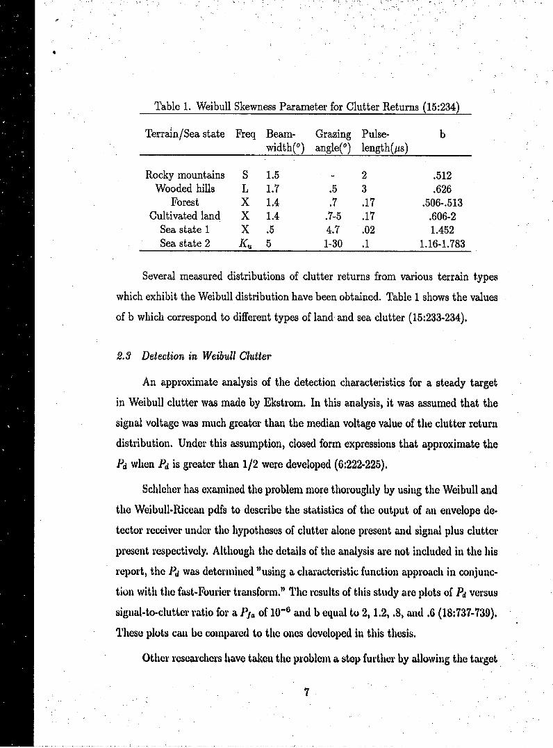
Table 1. Weibull Skewness Parameter for Clutter Returns (15:234)

Terrailn/Sea state Freq Beam- Grazing Pulse- bwidth(O) angle(O) length(ps)

Rocky mountains S 1.5 - 2 .512Wooded hills L 1.7 .5 3 .626

Forest X 1.4 .7 .17 .506-.513Cultivated land X 1.4 .7-5 .17 .606-2

Sea state 1 X .5 4.7 .02 1.452Sea state 2 KI 5 1-30 .1 1.16-1.783

Several measured distributions of clutter returns from various terrain types

which exhibit the Weibull distribution have been obtained. Table 1 shows the values

of b which correspond to different types of land and sea clutter (15:233-234),

2.3 Detection in Weibull Clutter

An approximate analysis of the detection characteristics for a steady target

in Weibull clutter was made by Ekstrom. In this analysis, it was assumed that the

signal voltage was much greater than the median voltage value of the clutter return

distribution. Under this assumption, closed form expressions that approximate the

Pd when Pd is greater than 1/2 were developed (6:222-225).

Schleher has examined the problem more thoroughly by using the Weibull and

the Weibull-Ricean pdfs to describe the statistics of the output of an envelope de-

tector receiver under the hypotheses of clutter alone present and signal plus clutter

present respectively. Although the details of the analysis are not included in the his

report, the Pa was determined "using a characteristic function approach in conjunc-

tion with the fast-Fourier transform." The results of this study are plots of Pd versus

signal-to-clutter ratio for a Pp, of 10- and b equal to 2, 1.2, .8, and .6 (18:737-739).

These plots can be compared to the ones developed in this thesis.

Other researchers have taken the problem a stop further by allowing the target

7

to be a fluctuating one. Goldstein obtained expressions for the Pd of a Rayleigh

target in Weibull clutter. These results are based on the assumption that the signal-

to-clutter ratio is large. For fluctuating targets, the pdf of the envelope of the received

signal when both target and clutter are present can be approximated by the pdf of

the target signal's envelope when the signal-to-clutter ratio is large (9:90-91). Chen

and Morchin also used this fact in developing an expression for Pd of a Rayleigh

target in Weibull clutter. Their results were plotted for b equal to .5, .6, .7, -and

.8 (3:929-932).

o" 8

III. Development of Detection Characteristics

The problem of detecting a signal known exactly corrupted by Weibull clut-

ter interference can be approached by first examining the detection problem of a

deterministic signal immersed in Gaussian noise. When white Gaussian noise alone

is passed through a narrowband filter, the probability density function (pdf) of the

envelope of the output noise voltage is Rayleigh. The envelope of Gaussian noise plus

a deterministic signal passed through a narrowband filter is distributed according to

a Ricean pdf (19:23-27). These results will be useful in the analysis of the detection

problem in Weibull clutter.

3.1 Rayleigh-to- Weibull Transformation

A Rayleigh random variable, r, representing the envelope of a narrowband

Gaussian process can be transformed into a Weibull random variable, w, by raising

r to a power, Y (8:10-11):

w=lrI (1)

The value of v that will result in w being a Weibull random variable is found by

performing the transformation of equation 1 on r. The variable, r, has a Rayleigh

pdf as shown:

p(r) = (r/a2 )exp(-r2/2a 2 ) r > 0 (2)

The parameter, a2, is the mean-square voltage of the Gaussian input. The pdf of w

is found as follows

p(w) = IW/") dr/dw

- (w(2/-1)/ra2) exp(W2/11/2a2) w > 0 (3)

A Weibull pdf has the form

9

signalSignal

_ ~ ~Gaussian • - BF Filter

noise

SignalEnvelop Thesol-Detector .Device 'sSignal

Present

Figure 1. Detector for Deterministic Signal in Gaussian Noise

p(x) = (b/a)xb-1 exp(-xb/a) x > 0 (4)

From equations 3 and 4, it can be seen that w is Weibull when

_ =2/b (5)

3.2 Detector Model

The Weibull envelope clutter process can be modeled artificially by modifying

a detection scheme used to detect a signal known exactly with unknown phase in

Gaussian noise, A simplified block diagram of a detector to detect exactly known

signals with unknown phase in Gaussian noise is showu in Figure 1 (5:298-302).

10

s l MaSchid neaoplSGaussian Filter Detectorr

enoisen

Signal1!w(t) , Threshold 7" Absent

S~()2/b =

-- b Device Signal

Present

m|j

Figure 2. Detector Model for Deterministic Signal in Weibull Clutter

Using the results of the previous section, it is seen that a Weibull process

can be simulated by introducing an operation after the envelope detector that will

transform the the Rayleigh variable, r, into a Weibull variable, w, when noise alone

is present. The operation necessary is determined from equations 1 and 5 and is

given by

-w = (6)

A block diagram for this detector is shown in Figure 2.

Use of this model allows one to approach the detection problem of a deter-

.ministic signal in Weibull clutter by first taking advantage of the well-documented

results of the detection, of a deterministic signal in Gaussian noise.

11

3.3 Radar Parameter Calculations

3.3.1 Probability of False Alarm. When there is no target signal present,

the signals, r(t) and w(t), from Figure 2 are distributed according to Rayleigh and

Weibull pdfs respectively. The pdf of w(t) is

p(w/Ho) = (b/a)wb-1 exp(-wb/a) W > 0 (7)

where H, represents the hypothesis that no target is present. The parameter, b,

indicates the degree of skewness in the distribution and a is related to the median

of the distribution (15:234). While b is determined by the type of terrain causing

the clutter returns, a is determined by the mean-square voltage, a2, of the Gaussian

input. It can be seen from equations 3 and 4 that a = 2a 2 . The parameter, a, is

related to the median by (1:2)

Wm = (aln(2))'I/ (8)

where w,, is the median. From equation 8 and the relation that a = 2a2, it is seen

thatoa 2 W'm/(21ln(2)) (9)

The probability of false alarm is determined by integrating the pdf of equation 7

from the detection threshold, wT, to infinity:

PjA =L b/a~w'- exp(-w 6/ct)dw

= exp(--w/2) (!0)

When Pj, is a fixed parameter, w2' can be solved for:

W2= (21n(1/.Pj.))/ 6 (11)

12

3.3.2 Probability of Detection. When an exactly known signal is present at

the input of the detector, r(t) has a Ricean pdf. Using DiFranco and Rubin's nota-

tion, the Ricean pdf is

p(r/Hi) =rexp[-(r2 + 7)/2JI0(rvrI-) r> 0 (12)

where H, is the hypothesis that a signal is present and IO() represents the zero-order

modified Bessel function of the first kind. IZ is defined to be 2E/No where E is the

detected target signal energy and N0 is the one-sided power spectral density of a zero-

mean white Gaussian noise input. DiFranco and Rubin refer to the parameter, 7Z, as

the peak signal-to-noise power ratio, which is the ratio of maximum instantaneous

signal power to average noise power out of a matched filter. T? appears often in radar

literature (5:302-307).

When a signal is present, r(t) undergoes the transformation of equation 6 and

w(t) has the pdf developed below:

P(w/Ihl) Al- = /0") 1 dr/dw I= Wi/U xp[-(,w2I• + #R)12]Io(W1IU. 1/)( 1l/)w(11"-1

- (w,(21b)-H/v)exp[-~(w, 2/ + ')/2]Jo(wl/U•) w> 0 (13)

Substituting P = 2/b, p(w/tfh) becomes

p(w/1I) (b/2)wb- Oxp[-(Ib + TZ)/2]J4(wb/I/i-) w > 0 (14)

To determine the probability of detection for a signal known exactly in Weibull

onvelope clutter, equation 14 is integrated from the de-tection threshold, w27, to

infinity:

1a1 J(b/2)w- cxp[--(wb.+ -?.)/2]l4(wb6 2/v.)dw (15)

13

This equation is of the form of Marcum's Q function given by (14:40)

•=0

Q(a, P) = vexp[-(v'2 + a,)/2]1C(av)dv (16)

Making the following substitutions:

ai=V

= WT

dv = (b/2)W(-1 2)1 dw

the integral of equation 15 can be written as

Pd ,vexp[-(v2 + Z)/2]Ilo(vvrI-)dv (17)

- Q(--. WT) (18)

Combining equations 11 and 18, Pd becomes

Pd = Q(V•, (2ln(1/Pj,))"'/) (19)

Also, Maxcum's Q function can be written in teris of the incomplete Toronto fuac-

tion as (12:160)

Q(,) =.1 -7 (1,0, v2) (20)

Therefore, Pd becomes

Ia 1 - 212u(Ijj))16/vr2(1, 0. (2/2)'/') (21)

When b = 2, it is smen that the pdf of w(t) is Rayleigh and the Pd and P1-. arethe saue as thos- found for the case of an exactly known signal with unknown pha.e

14.

detected in the presence of Gaussian noise with an envelope detector. Several texts,

including DiFranco and Rubin's contain plots that show the required peak signal-to-

noise ratio, IZ, needed to acheive a desired probability of detection for various values

of false alarm (5:308). These plots axe identical to the ones that would be created

by an evaluation of equation 19 with b = 2.

3.4 Relationship between SCR, P1 a, and Pd

In the case of the detection of a deterministic signal corrupted by Weibull

clutter, b is typically not equal to 2 and Pd is determined by equation 19 or 21.

When the target signal is corrupted by Weibull clutter, it is more meaningful to use

a signal-to-clutter ratio (SCR), instead of the parameter, 7X.

The clutter power is determined from the second moment of the Weibull pdf

of equation 7 as (15:34)

2

E[w2] = IP(1 + (2/b))(ln 2 ,b (22)

where r0 is the Gamma function and w,,, is the median of the Weibull distribution.

If the implitude of the signal before the envelope detector is A, the power signal-to-

clutter ratio at point b of Figure 2 is

-s5cb = (A 21 b)2

-(wz./(l 2)2/b)r(l + (2/b))

= (AS) 2/b(In 2)2/b (23)w2, (1 + (2/b))

Recall that 7R is the peak signal-to-noise powe.r ratio. The pe"-k signal power

is relat Wd to the average instantaneous power by (5:296)

(peak instantancous signal jower) 2(average instataneouw sigwl powr)

(24)

The average instantaneous signal power of a sinusoidal signal of amplitude, A,

is A2/2 and the average noise power is a2 . Therefore, RZ expressed in terms of a 2 is

1? = [2(A'/2)]/a2

= A2/la2 (25)

Using equation 9, it is seen that

R ?= (A22 In 2)/wb (26)

Therefore, SCRb is related to 7R by

sc.•, = P(1 + (2/b)) (27)

To determine the SCR at the input of the envelope detector, the inverse of the

transformation of equation 6 can be performed on SCI4 to give

SCR? (s51)6/2

2[r(I + (2/b))jI62 (28)

This leads to

R = 2(SCR)[P(1 + (2/b))]61/2 (29)

VI = [2(SC)]•1'2[r(1 + (2/b))•1, 4 (30)

Comibining equations 18 and 30, the relationship between SCR, P1,, and Pd is

Pa = Q((2(5CR)I 2 [IX(I + (216))14, [2lu1/lPp)]ib) (31)

where q(&,#) is Marcumn's Q function.

16

3.5 Radar Range Equation

The radar range equation for targets in area clutter can be divided into two

cases: beamwidth-limited case and pulse-length-limited case. For large grazing an-

"gles, the area of terrain illuminated by the radar is limited by antenna beamwidth;

"while for small grazing angles, the area is limited by the pulse-length of the trans-

mitted signal. The radar range equations for each of these two cases are (16:63-67)

R 2 = L(sint¢)o't qSR"R2 = /4)0(SCR)00 for tan 0 > cO/2 (32)

andL(cos 0) at _4?

?= S (cs/2)0 for tan 4 <-- (33)SR=(SCR)(c•/l)Ooo

where

* L, all of the various losses encountered by the radar

*.41 = grazing angle of the radar

o •x = taxget radar cross section

*. SCR = mean sigrad-to-clutter power ratio

!a,, the backAcatter (clutter) radar- cross section per unit area of reflectingsufcce (int/m2) ,

*. 0 =.d3-dB beainwidth in azimuth

... " .c• t width ianelevation

*:r T P44o duration of the trans•aitted sigeal

: Spixa1 of lightS .: =: :* It = raulat det.cion .range

ThS•itc�h It e solvexd fol to 'obtain

.. ,*:.v,.: :&j)4' t y "j- •' .for taaa' (3,4)

1061

: ' """'"'=Tf• "'--" " t

and

SCR= L(cos I)ro for tan4€ < OR (35)R(c~r/2)0a0 cr/2

Now, define a normalizing range, R., which is the range at which the SCR becomes

unity (2:23-27). Using equations 34 and 35, RA becomes

Ro = .(L(sin / b)a 1/2 tan ¢' O/R (36)-, for c, r/2

and L(cos V)ut for tan 0 < -R- (37)

= (cr/2)0o0 cr/2

Now, all radar parameters axe included in X0 and SCR can be related to range readily

by

RlBo = (1/SCR)1/2 for tan 0 >OR(8cr2 (38)

and

R/IB = 11SCR for tan 0 < (39)c(39)

Therefore, for small grazing angles (pulse-leugth-limited case), the detection

range' is inversely proportional to the SCR.- For la'ger grazing angles (beaniwidth-limited ease), the detection range is inversely proportional to the squaxe root of the

.l .ca e) t-.de.....r

The relationship between detection rangp, P,, and P1. -ca, be determined by

combining equations 31, 38, and.39:. "

• • p•= Q(x/(14/R)[jPQ + (2/b,))][16/,(I(•1/,,)j]1/) fer tanl 4> •"•. R 0-for UUtP >(40)• ; ~' .r/2

Wvhere ~i 4)~

(41)

S' . .. k ,,-/ )o~k o) ...8

aand

Pd = Q((2Ro/R)l/ 2 [r(1 + (2 /b))]4 r[21n(q/Pp)] b) for tan' < ýR/ (42)

~~j~IJL + I)Ji L 1 ~/fJJ)cr-/2

whereR L(cos b)ot (43)

(cr/2)0ao

Equations 40 and 42 along with equation 31 can be evaluated to obtain plots

of Pd versus R/Ro and Pd versus SCR for various values of P1 . and b. The detection

problem becomes a problem of evaluating the Q function for the arguments shown

in equations 31, 40, and 42. This is the subject of Chapter 4.

19

IV. Computer Implementation

The expressions for Pd from equations 31, 40, and 42 describe the detection

characteristics of a steady target in Weibull clutter. In order to evaluate these

expressions, a means of tabulating Marcum's Q function must be developed.

4.1 Algorithm to Compute Q function

In a Johns Hopkins University report by Fehlner, an algorithm for computing

Marcum's Q function was developed. The integrand of the Q function was red-

erived using the characteristic function and the Q function was finally expressed as

a series (7:23).

The characteristic function for Marcum's Case 0 is the Fourier transform of

the integrand of the Q function of equation 16. First, the substitution, u v2/2 amd

du = vdu is made to obtain the integrand, I:

1 = exp[-(u + a2/2)]o,(av/u) u > 0 (44)

The characteristic function becomes

C = jo exp[-(u + a2/2)/o1(c)V2ei)ddu (45)

Letting x = a2 /2 and p = jw, C becomes

C -- exp[-(u + x)]l°(2vru)eP"du (46)

Marcum found this integral to be (12:1634164)

C [1/(p + 1)]e'- Oxp[x/(p+ 1)] (47)

20

Fehiner takes the inverse Fourier transform by contour integration and obtains

f_---=;(1/2 rj)11 e- exp[x/(p + 1)] exp[(p + 1 - 1)t]f (t) = (1/2rj) J-,'OO P + d pe- e- 00 exp[-x/(p + 1)] exp[t(p + 1)1]

= e ....... Ldp (48)

Fehlner's evaluation of this integral results in

00

f (t) = E-• Z(xli!)(t/i!) (49)i=O

Now, to determine the Q function, the integral

f (t)dt (50)

must be evaluated, where uT is the threshold corresponding to f6 from the original

expression for the Q function. Upon evaluation of this integral, Fehlner's final result

becomes a series expression given by (7:24-25)

Q(X,U2') = •-•E (Xi/f_ i!)•(e-"UT/j!) (51)i=O j=O

Recalling that x a2/2, u v2/2, and thus UT = p 2/2, equation 51 becomes

00 •= •2)i (p2/2)j (52)i=o j=O

This series can be carried out to the desired precision.

4.2 Computational Problems

It caa be seen from equation 19 that as b and 1-,, are decreased, the second

argument of the Q function, P, becomes large. Also, as the SCR is increased, a, the

first argument-of the Q function, becomes large. Large values of a and/3 become

21

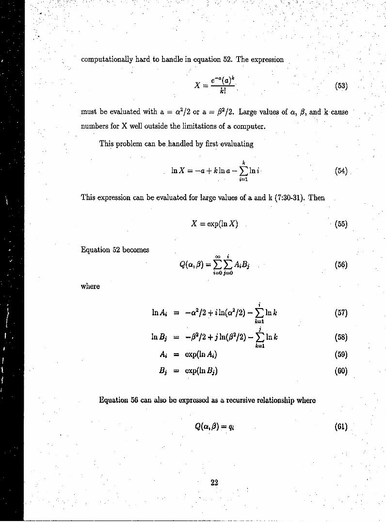
computationally hard. to handle in equation 52. The expression

X eaak (53)

.must be evaluated with a -a'/2 or a =p 2/2. Large values of a, /,and k cause

numbers for X well outside the limitations of a computer.

This problem can be 'handled by first evaluating

A:InX=-a+klna-Zlni. (54).

This expression can be evaluated for large values of a and k (7:30-31). Then

X =exp(In X) (66)

Equation 52 becomes 0

Q = ~p) jE AiB3 (56)i=O j=O

where

In Ai -a a2 /2 + i ln(0v2 /2) - Ink (57)

In B3 -P/ + i lu(P 2/2) - In k (58)

Ai= exp(In A,) (59)

Ii, = exp(lu B,) (60)

E~quation 56 can also be expressed as a. recursive relationship where

Q(cv 1P) =i (61)

22

The initial value of q is computed as follows

InA 0 = -a 2/2 (62)

BIn = -p 2 /2 (63)

A0 = exp(ln Ao) (64)

B, = exp(ln B0,) _(65)

qo = AoBo (66)

The other values of q are computed from

lnAi = InAi-. + ln(a 2 /2) - Ini (67)

lnBi = inBi-. + ln(/32/2) - ini (68)

A, = exp(InAi) (69)

Bi exp(1nBi) (70)

q= qj-1 + AjB, (71)

The value of i in equation 61 must be large enough to cause Q to converge to

the desired accuracy. To obtain a six digit acurracy, i must be large enough that

.qi-i/q > .999999 (72)

4.3 Computer Program Design

The FORTRAN computer program found in Appendix A was developed to

produce data that can be used to plot Pd versus SCR and Pd versus R/RX for

different values of b and PfG. The input to the program includes: the value of b,

the value of P10 , and whether the grazing angle is large(beamwidth-limitcd case) or

sxnall(pulse-length-litnited case).

The prograim, evaluates equation 19, which is Pd expressed as the Q function

23

of ()Z)1/2 and [21n(1/Pa,)]1/b. First a and fi are computed according to equation 19.

Then equations 62 through 66 are used to determine qo. Then, a DO loop is carried

out to determine q, according to equations 67 through: 71. The loop is exited when

the inequality 72 is satisfied. Next, R• is converted to SCR according to equation 29.

This conversion involves the Gamma function and the GAMMA function provided

by the International Mathematical and Statistical Libraries (IMSL) is utilized in the

program (10:GAMMA-1). R/RO is then computed according to equation 38 or 39.

The Pd, SCR, and R/1o are output when Pd is between .0001 and .9999. Finally,

7R is incremented and the computations are repeated until Pd becomes greater than

.9999. The flow chart describing the program is shown in Figure 3.

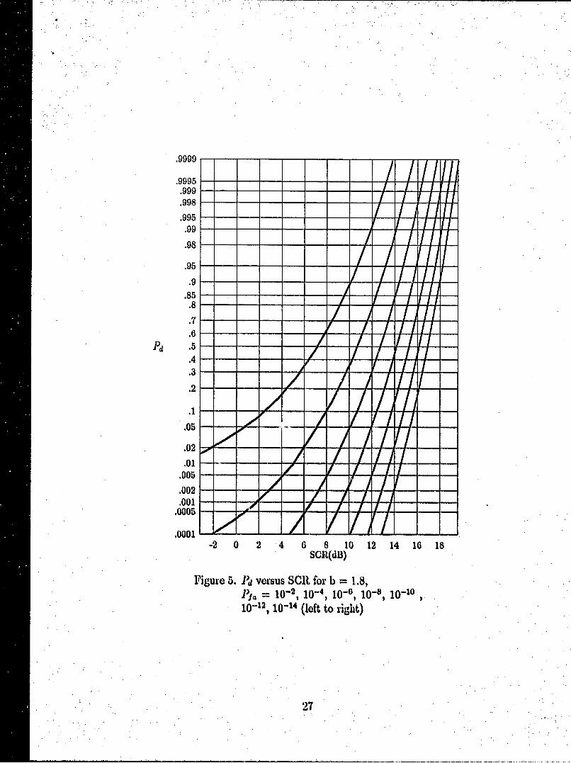
Figures 4 through 12 are plots that show the required SCR needed to produce

a desired Pd for various values of b and Pf a. Figures 13 through 21 are plots of Pd

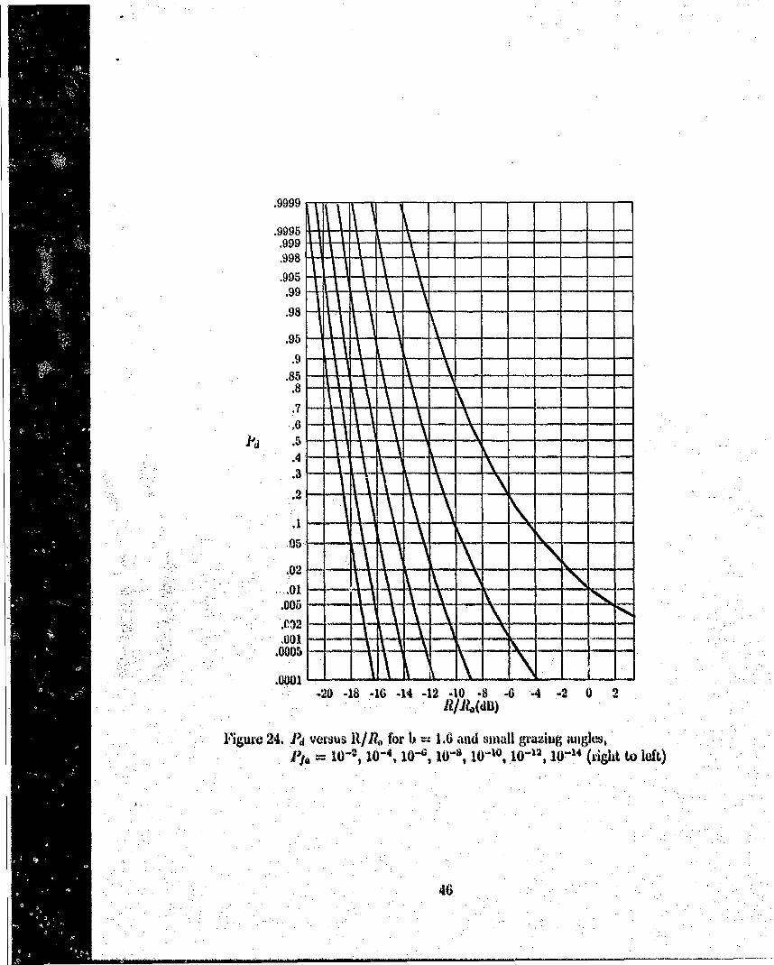
versus R/Ro, for large grazing angles and Figures 22 through 30 are the same plots

for small grazing angles.

As Pja and b become small, the number of iterations required to cause the

summation of equation 56 to converge becomes extremely large. The computation

time required to evaluate the algorithm for small values of b and P1 o also becomes

extremely large. This is why in Figures 11, 12, 20, 21, 29, and 30, the number of val-

ues of Pp, are limited. The skewness parameter, b, is reduced to .5 in Figures 12, 21,

and 30. Values of b smaller than .506 are not documented.

24

Input: Initialize Compute

biffa)angle 1Z alp

Compute

qO

Computeqj

qi-i/qi>.999999No

Yes

r Convert R

to SCR

Angle? -Small Compute

<

I SCR

Large j' (ComputeRlRo=ll(SCR) 1/2

.0001<pd<.9999 Yes Output:SCRIR/RoPd

No

>.9999 Stop

Increment

7Z

r, igure 3. Prograin Flowchart

25

.9999 --

.9995 -- 17.999 -4-.998 EMU

.995 --

.98 --

.95 -- -

.9 - -- - --

.85 --

.8 --

.07

.00

.0001

.0 20 -0 - - - - -

.0001, 144(et orgt

26

.9999 --

.9995 -- -.999~.998-

.995 --

.99 --

.98 --

.95 1 -A-

.9 --

.85-.8--.7 -

Pd .

.3 -- - -

.2 - - - --- -

.05 - -z-

.02 - -oor

.005 - - --- -

.002 -0o - -- z-

.001 - -- -- -

.0005--

.0001 - - --

-2 0 2 4 8 8 10 12 14 16 18SCR(dB)

F igure 5. Pad versus SCR. for b 1.8,=f 10-21 10-11 10-6$ 10-82 10-101

101, i0-14 (left to- right)

27

.9999 - - - - - - - - - --

.9995 ---- -

.999 - - - - - - --

.998 - - - - - - - -

.995 --

.99 --

.98 --

.95 ----

.9 --- --

.85 --

.8 -- -

.7--

.6--

Pd .5

.2 --

.05 -- - -- -

.01 --00-

.006 -- ---

.002- - - --

.001 - -- -.0005 -~-

-2 .0 2 4 0 8 10 12 14 16 18 20SCR(dB)

Figure 6. Pd versus SCR for b 1.6,

1O-12 1i-1 (left to right)

28

.9999 ,.

.9995 --

.999 --

.998 --

.995- -.99 - -

.98 - -

.95 i I I

.9 - ll-.85 - -

.8 ---

.7 -

Pd .5 - 1 11 1.4 --- - -

.3--- -

.05 --- - 1

.o1 - - 1 - I -/ l

.02-----------

.01------------.005--- - 1 -

.002 . . . -' /-

.001 , - - - - - - - -...- -.10005- - ---

.0001-----------------------2 0 2 4 6 8 10 12 14 16 18 20, 22

Figure 7. PI versus SOCR for b = 1.4,: " ])I,• "-" l -l 10-4, 10-111 10-11 1O'0-".".0

"10=12 10-1i (left to right)..

29

.9999

.9995 -.999 ---

.998 --

.995 - -

.99-- -

.98------

.9 -5 - - - -I-

.85 - -I.8 1 -I

.7 - - -- -

.6---P', .5

.4-. -

.3-- -

.05 --- - - - -

.02 - -- -

.005-- - - -i -

.002

.001 --

.0005- -

,5 7 9. o.11 13 15 17 19 21 23 25 27SCR(dU)

_•! •.Figure S."lPd ,'ersus SCRt for b 1.2,, .. : .. ..p/. = 10-2 10-4, ý 10•o 10-, O- ,

, " .. .! - '" (left to righlt)

30

.9999 - - --

.9995--- --

.999-- --

.998----

.98-- -

Pd 6

.3-'

.102- -

1 1t Ila 18 20: 24. ýi4 20 28 3O a

F) gure . Pl Vrsus SCRI for' 1 ) ": ,

iolC o 0,1

W12 10 OUR 1

.9999 -

.9995 - -..999--m x.998 - -

.995 - - - - --

.99

.9 --

.7- - - -- - . -

.1-

'102

.9999 - - - - - - . - .

.9995- -- - -

.999----

.998--- ----

.995 1- - - - - - - - --

.99--e.--,-'-.

.98- - - - -

.95 - - -

.9 - - -

.85- - - -

.8- - - - -

.7.-. . . .-

PC, .5

.4 --

.3-- - -

.2 - -

.01.05 -

.002

.001 ~

.0002

.0001 - - - - - - - - - .

27 20 31 33 35 37 39 41 43 45 47 49

F-igure I. Pd9 versus S., for b .6,

-10-1 1 10-01 0-S, 10-10(left to right),

A J33

.9.9999

.9995.999.998

.995.99

.98

.95

.9

.85.8

.7

.6Pd '

.4*.3 --

.2

.05 ---

.02 . ..-;.01--

,005

.002.001 - ..

.0005

.000132 34 36 38 40 42 44 46 48 50 52 54 506 8 60

SCR(dB)

Figure 12. Pd versus SCR for b = .5,P1a = 10-2) 1071, 10-1, 10-8, 10-10(left to right)

~34

.9999 , - ,

.9995 -.

.999-.998-

.995 -\-

.99- -

.98 -\

.95 .- -

.9 -- - -

.85 -- -- - -

.8-

.7-

.6 -

Pd .5 -

.4

.2 -

.05 - - --

.02

.01- - -.005 - - - --

.002 - -

.001 - -- -- -

.0005 --

.9 8 .-7 -6 -5 -4 -3 -2 -1 0 1R/R0 (du)

Figure 13. Pd' versus R/R0 for b = 2 and large grazing angles,P = .10-2 10 -1 10 - 100-81, 10-1o, 10-1, 10-14 (right to left)

-. .. . .3o

.9999 --

.9995- - - - - - - -

.999- - - - - - - -

.998- - - - - -

.99 --

.98- -

.9 -- -

.85-

.7-

.6 --- - --

Pd .5-.4--.3-

.2 - --- -

.05---

.02 -

.01 - -

.005 - X-

.002 ---

.001 1 x- A--

.0005 - - -

.0001 - -

-9 -8 -7 -6 -5 -4 -3 -2 -1 0 1R/RX(dB)

Figure 14. Pj versus R/R,0 for b =1.8 and large grazing angles,=l 10o , i0,1- '101,w i0-8 10-10t 10-12, 10-1 (right to left)

.36.

.9999 -- -

.9995-- - - - . - - -

.999 - - I .

.998 - - - - -

.995 - - - - -

.99- - - - - - - -

.98- -

.95 -- -- -

.85-\- -

.8-

.6.5

.4 -- - -- - - -

.3-

.2 -4---

.1 - - - ,- -• -

.05-----

.02.-.- - -A

.01 • -.005 - -

.002 ----

.001 - - - - - - - - - - - -

.0005--11

.0001 - -

-10 -9 -8 -7 -6 -5 -4 -3 -2 -1 0 1R/R0 (dB)

Figure 15. Pd versus fl/Ri0 for b = 1.6 and large grazing angles,=J 10-11 10-4 10-111 10-1 10 -0 10-12 1iQ1-1 (righit to left)

37

.9995 -

.9995

.998 .-- -

.995 - , -

:.99 .- ,

.98 -I

.95

..99

P .d l l -I i I -'"-.8 |

.7 f l

.4 l - -. - . ..

.3- - -

.I I ~I AIl\

.02-1,o -I-

.01-.005

.002- - - - - - - - - -

.0 0 15 -N ..-- - -

.0005 - -

.0001--o__\--11 -10 -9 -8 -7 -6 -5 -4 -3 -2 -1 0 1

R/Io(dB)

F igure 16. Pd versus R/RO for b = 1.4 and large grauing angles,P /91= 10-2, 10-1, 1061 10-"8) 10-101 10-12, 10-14 (right to left)

38

.9999 --- - - -

.9995--.999--

.998

.995--.99--

.98-

.95

.9.851

.8 ----

.7- -

.6 -- --

Pd -5- --

.4-- --

.3--

.2- --

.05 --- --

.02 - - --

.01 -' -

.005 -----

.002-.001 -.

.0005- - - - - -

.0001--- --

-13 -12 -11 -10 -9 -8 -7 -6 -5 -4 -3 -2R/Ro(dB)

F igure .17. Pd versus R/RO, for b = 1.2 and large grazing angles,=10-21 10-1 10-11 10-11 10-101 10-12, 10-4 (right to left)

39

.999 - - __- - -- - -

.998-_--

.995 .-- -

.99 - - -

.98 - I -

.95 - I_.9 - - - -

.85 - I -

.8 - - --

.7 -

.6 --- --

Pd .5 -1

.4 - --

.3 - - -

.2 . .. ..

"°.1 - -I--I

.05 ---- - --

.02-----_-o0

S-~~.16 -1,- -4 - 3 - 2 -1 -0 -9 8 -7 -

.010

.005---

.002---

.001----.0005--- -

.0001 - - - -

-16, -15 -14 -13 -12 -11 -10 -9 -8 -7 -6R/Ro(dB)

Figure 18. Pd versus ft/R, for b = 1 and large grazing angles,=l 10-21 10-11 10-1, 10-11 10-10t -10-12, 10-14 (righ~t to left)

-40

.9999

.9995.... 998

S.9998 --

• .995

.99

.98

.95.9

.85.8

.7

.6

Pd .5.4 -

.2 -

.05

.02 - - - - - - - - - -

.01.005

.002 .--. .,001 ......

.0005 - - --

.0001 L I-20 -19 -18 -17 -16 -15 -14 -13 -12 -11 -10 -9

_R/X(dB)

Figure 19. Pd versus R/R. for b .8 and large grazing angles,PIG, =10-2, 10"4 10-6, 10,1- 1010 -1012, 10-14 (right to loft)

41

.9999 ---

.9995.999.998

.995•.99 - - - - - - - - - -

.98

.95

.9

.85.8

.7

.6Pd .5

.4

.3 - - - - - - - - - - -

.2 L---

.02

.01 --.005

.002

.001 - -. . ...- -.0005

.0001-24 -23 -22 -21 -20 -19 -18 -17 -16 -15 -14 -13.lt/R 0 (dB)

Figure 20. Pd versus R/Jo for b = .6 wid large grazing angles,Pa 10-.', -0"-, 10-6 10-8" 10-10 (right to left)

-42

.9999

.9995 -.999 -.998 -

.995.99 -

.98 -

.95

.9.85.8 - -

.7

Pd .5. ..

.4

.3

.2

-- - - -0,- -

.05 - - - - - - - - --

.02

.01 - - - - - - -- -

.005

.0022--,001 - -

.0001 - ---20 -27 -25 -23 -21 -19 -17

Figure 21.. Pd versus R/R. for b = .5 mid large grazing angles,Pla 102, 10"4t 1001, 10"8, 10-10 (right to left)

43

.9999-

.9995 - -

.999-

.998 -

.995 -

.99

.98 ~

.95 -

.9 - ,-

.85 --- - - - -

.8 --- - - - -

.7 - - - - - -- ~ ~~.6 X\ X i\' , .. .Pd .5 -

.4 - -- - - - -

.3 - -

.2-,

.05 ---

.02--

.002- -

S_.805 - ---- -,

.0 0 1 -s- -

.0001 . -.- \ . -

-17 -15 -13 -'1 -9 -7 -5 -3 -1 1 3S::R/R•(d X)

Figure 22. P1g v-rssus RI/R for b = 2 and small grazing angles,---- ." P 10A ,1041 10-6, 10-1, 1",0-1 10 10-14 (right to left)

44

.9999--- - -

.9995 - -

.999- --

-. ,~~~~~~998----------------------.995-

.99- -

.98-

.95 - - - - - - -

.9-- .

.8-

.7-

16 14I -L12 -10- -

'.4. 10 1-. -o -!t -0

.9999 --

.9995---.999 -

.998- -

.995--.99 -

.98

.4-

.0056-- -4 7

.0001 .- -

-20 -1. .-IG 414 -12 -10 -8 -6 -4 -2 0 2

Figture 24. J', versus It/&- for 1) 1.6 and smnall graxing migit~s,la 10-2. 10-4, 10Ofi 10-11 1- 1,01 10-12 t lo- 4 (right to left)

46.

.999.--

.995..99 -

.98

.95- -- -

.9 N..- -

.85 -

.8 --- - -

.7 -

.6 - \ -

Pd . - - -

.4 - - - . .........

.2 I... 1, -l l - -\ -

.05 .

.01 .1005-

.002-

.001 - - - . - -. . -

.0005

.0001-.2•.-218-16-14-12-10 -8 -0-4 .2 02

F.igure 25. P.1 versusn R/&o for Ib 1.4 and small graiug magles,.Pp 10", 1 -, 1O", 08, 10-10, 10-1, iO- (right to Ilo)tV .d .1:0

.9999--

.9995 -t I-.999 I -I-

.998 -

".995 - -

.99-

.98

.95-.9

.85 - -

.8 - - .

.7-

.6 lPd - -5

.4-.--

.3---

.2--

.05-

.02-

.01 ---

.005 -- - -1 l-

-.002 --

.001 - -

.0005

-26 .24 -22 .- 20 -18 -16 -14 -12 -10 -8 -6 -4Rt/,4,(dB)

Figure 26. Pd vesus R/I, for b 1.2 and small grazing augles,pin = 10-2, 10"4, 10O6, 1O1-, 10"10, 10-12, 10"14 (righlt to left)

48..

.9999 - - - - - - - - - - -

.9985 ---

.995----.995 I-

.98 II

.958 I.995 I

.85 - - -

.8 -

.7 . - - -

.6 ---

Pd .5 ---

.4 - -I - -...

.3 - --- --

.2 -- - -

.1 i-- - .

.05 --

.02-- -

.01- - ---

.005 -----

.002---- -' -

.001---.0005

.0001-----31 -29 -27 -25 -23 -21 -19 -17 -15 -13 -11

R/&R(dB)

Figure 27. Pd versus R/R0 for b = 1 tand small grazing amgles,I = 10-2, 10-4, 10-1, 10-8, 10-t0, 10-12, 10-14 (right to left)

.49

.9999-'- . ..-- -. ! 1: ,..

.9995- - -.9999.998-

.995.99

.98

.9.85 - -

.8 -1

.7 -

.6

Pd -4 .4

.3-. .

.2o -

.0 5 . . . .... . . ....

.02- - - - - - -

.005-

.002 . . . . . . .

.001.0005

.0001o-o-39 -37 -35 -33 -31 -29 -27 -25 -23 -21 -19 -17

R/1'(duI3)

"Figure 28. Pa versus R/14 for b = .8 and small griaing angles,P. 0 10- , 10-41 10-, 10-, 10"- , 1 0- 10-110-14 (right to left)

50

.9999 - - - - - - - - - - - -

.9995 - - - - - - - - - - -

.999 - - - - - - - - - -

.998 - - - - - - - - - -

.995 - - - - - - - - - - -

.99 - - - - - - - - -

.98 - - - - - - - - - - -

.95 -

.9 - - - - - - - - - - -

.85 - - - - - - - - - -

.8 - - - - - - -

.7 - - - - - - - - - - -

.6 - - - - - - - - - - - -

Pd .5 - -

.4 - - - - - - - - - - -

.3 - - - - - - - - - -

.2 - - - - - - - - - - -

.05 - - - - - - - -

.005 - - - - - - - -

.002.001 - - - - - - - -

.0005 -

.0001 - - - - - - - - - - -

-48 -46 -44 -42 -40 -38 -36 -34 -32 -30 -28 -26

Figure 29. Pj1 versus R/R0, for b =.6 and sm~all grazing angles,p 1O-11 10',1 10-61 10-8,1 10-10 (right to left)

.9999-

.9995 - - -

.999-- - -

.998 - - . --

: - - - . "-. , .. .' '

P..6 -. "-- • "

. 5 - - ..-

•1 . - - . - - -

.9959'

.989 . .

.999. . ..

98

.00

P I.-5---.-.-4

Fiue3.P eru /? o b ,5 im gaiI g nls

.22

.05

.02

.0

Pd .5 9 -5,5 53 14 -47 -45 -4 -4 3 3 3 3

,f2 i1- i 10 4ii-110 1,1 -0(igh to. let

52i

-4.4 Results

4.4.1 Validation. In order to determine if the curves presented are valid, the

curves developed for b =2 can be compared to those presented by other authors

who analyzed the detection problem of a steady target in Gaussian noise. When b

=2, the pdf of the envelope of the interference is-Rayleigh as seen from equation

7, and Rayleigh envelope interference corresponds to Gaussian noise at the input

to an envelope detector. Therefore, the detection problem for a steady target in

Weibull clutter with b 2 is identical to the problem of detecting a steady target

'in Gaussian noise. DiFranco and Rubin's curves of Pd versus the peak signal-to-

noise ratio for the Gaussian detection problem are identical to the curves shown in

Figure 4 except for a 3 dB shift in the peak signal-to-noise ratio axis (5:308). This

discrepancy is explained by noting that the curves in Figure 4 are plotted with the

mean signal-to-clutter ratio, SCR, on the x-axis while DiFranco and Rubin uise the

peak signal-to-noise ratio, 1Z. From equation 28, it can be seen that when b =2,

SCR = Rj2, thus the 3 dB3 discrepancy.

To further validate the curves, they can be compared to the results obtained by

Schleher. Schleher developed plots of Pd versus SCR for a steady target in Weibull

clutter for Pi. = 10-6 and b = 2, 1.2, .8, and .6 (1.8:737-739). These plots correspond

to the curves shown in Figures 4, 8, 10, and 11 with Pj. 10-6 and the curves in

these figures match the ones developed by Scideher.

4.4.2 C~oinpanison of Results for Various Values of bi. From the results ob-

tained, it is seen that as b is decreased, or the skewness of the clutter distribution

is decreased, the amiount of SCR required to produce a desired Pd is increased and

thus the detection range is decreased. Table 2 shows the additional SCRt required to

produce a 11d = .9 With pi1 , = 10-6 when b is not equal to 2 compared to the Rayleigh

envelope case when b =2. The decreas e ini range for large and small grazing angles is

also shown. Table 2 shows that as t~he skewness of the clutter distribution is changed

-53

Table 2. Additional SCR and Decrease in Detection Range

b Additional Decrease in R/Re for Decrease in R/Re? forSCR(dB) Small Grazing Angles(dB) Large Grazing Angles(dB)

1.8 1.2 1.2 .61.6 2.6 2.6 1.31.4 4.6 4.6 2.31.4 4.6 4.6 2.31.2 7.4 7.4 3.71 11.6 11.6 5.8.8 17.8 17.8 8.9.6 28.6 28.6 14.3.5 38 38 19

(b decreases), the performance of the envelope detector receiver is degraded.

As an example of the performance degradation, one can compare the detection

characteristics found for two different types of terrain. Suppose b = .626 for terrain

characterized by wooded hills and b = 1.452 for the ocean (see Table 1). Using the

algorithm and computer program described previously, it was found that approxi-

mately 24.1 dB more SCR is needed to detect a steady target over wooded hills than

that needed to detect a steady target over the ocean. For small grazing angles, the

detection range is also 24.1 dB less for detection over wooded hills than the ocean

and for large grazing angles, the detection range is decreased by 12.03 d13.

54

V. Conclusions and Recommendations

5.1 Conclusions

The purpose of this thesis was to develop a means of predicting the radar

detection range of steady targets in Weibull clutter. This was accomplished by mod-

ifying a detection scheme used to detect steady targets in Gaussian noise and then

determining the relationship between Pd, Pfa, SCR, and b and finally applying this

relationship to a modified form of the radar range equation. The expressions describ-

ing the relationship between Pd, PJG, SCR, b, and range were found to be in the form

of Marcum's Q function (see equations 31, 40, and 42). Computer implementation

of the recursive algorithm presented in Chapter 4 used for the evaluation of the Q

function was capable of producing data used to plot Pd versus SCR and Pd versus

range for various values of Pf1 , and b. Six digit precision was used in developing the

plots but the algorithm is capable of providing greater accuracy.

The plots of Pd versus SCR developed in Chapter 4 describe the detection

characteristics of a steady target in Weibull clutter and show that the performance

of the detector is severely degraded as the skewness of the clutter distribution is

decreased. That is, as b is decreased, the SCft required to produce desired values of

Pd and P1. becomes large (see Table 2).

Finally, the plots of Pa versus R//X provide a means of predicting the radar

detection range for particular types of clutter (values of b) and desired values of Pd

and P10 . Several improvements can be made to this study and some are suggested

in the next section.

5.2 Recommendations for kAstuve Research

5.2.1 Weibull TAryjet. The next step in the Weibull clutter detection problem

is to allow the target to fluctuate. The Weibull pdf can be used to model the target"

•55 . -

just as it was used to model the radar clutter. Recall that the Weibull target model

is equivalent to the often used Rayleigh model when b = 2. The Weibull target

model is better suited than. the steady target model as an approach to problems like

detecting helicopters flying nap of the earth profiles. The following development is

provided as a suggestion on how to approach the analysis of Weibull target detection

in Weibull clutter.

With the problem of detecting a Weibull target in Weibull clutter, the pdf of

the detected signal under the hypothesis of clutter alone present is still given by

equation 7. When a target is immersed in clutter, the pdf of the detected signal

describes the distribution of the sum of two random processes. The pdf of the sum

of two random variables is the convolution of the individual pdfs (4:186-189). The

pdf corresponding to the clutter is

pc(w) = (bo/ao)wb°6- exp(-wb,/Ci,) w > 0 (73)

and the pdf corresponding to the target is

pi(w) = (bl/ai)wble:.rp(-wb1/cx) w> 0 (iA)

so the pdf of the signal under the hypothesis that atarget is preseat, becomes.

Apw/H) p0 (w),*p(w) P(Oh)W

Therefore the pdfs of the detected signal under the alternate hypotheses are

.pAw/1) (bo/ao)wb°- exp(-wb°/co) w > 0 (76),.:*.•:bob, t bV-I(W X), -1

p(w/I,,) i Wjo1,, -

exp(-WI,/a,)exp[-(w x)1/ail]dx (77)

- . . - .-

The parameters b0 and ao pertain to the clutter while b1 and a, pertain to the target.

The integral in equation 77 cannot be expressed in closed form, making it

difficult to determine the Pd. The integral can- be approximated numerically using

techniques such as the trapezoidal rule or Simpson's rule (11:368-390). The pdf of

equation 77 can then be evaluated for a range of values of w and the distribution

corresponding to the pdf of 77 becomes a discrete distribution.

Proceeding using a binary decision approach, the likelihood ratio, A(w), can

be written as

A(w) = p(w/Hj) (78)p(W/H,)

and the likelihood ratio test becomes

A A)._pw/HI) >,ffA() w/) < A (79)

where A is determined by the particular decision criteria that is employed. Using the

Neyman-Pearson decision criteria which requires tha;t A be determined according to

a preselected value of PI.. the detection threshold, wu, can be found by equation 11

anid A becomes (13:28-38)

.A =A(ti') (0

When dealing with discrete distributions, the Pd can be deteroned by sum-

ming up p(wi/IfI) for all i such that 4(wi) >.A(",) (17). That is

Pd. --Ep(wj/J1) such that. A(w,) > A(w 2-) (81)

where p(w 1 /Jl) is-determined from the numerical evaluation of euation 77, p(wj/H 0)

.is detemie�� from equation 76, A(wj) is determined from equation 'wi8, and tv can

is •oter e .. "

be any value between 0 and infinity. Equation 81 can also be written as

Pd = 1 - such that A(wi) <A(wT) (82)i

The details of performing the numerical integration, developing the discrete distri-

bution, finding the relationship between Pd, P1., and SCR, and applying the results

to the radar range equation are left to future researchers.

5.2.2 Other Recomendations. Future research should examine the target de-

tection problem with more than one observation of the returned pulse. That is,

instead of using single-hit detection, utilize pulse integration in the detection scheme

and examine the problem with multiple pulse observations.

Also, the problem could be extended by determining the detection characteris-

tics when other types of radar are used. A comparison of the detection characteristics

could be made for pulse, moving target indicator (MTI), pulse doppler, and contin-

uous wave (OW) radars.

5.3 Summaryj

By using the expressioos for Pd developed in Chapter 3 and'the algorithm for

evaluating thle expressions presented in Chapter. 4, the detection characteristics

of a, steady target in Weibull clutter can be determined. Pd can 'be found to .a

desired precision for varying values of SCR, R/&4, Pjo, ald b and plots can be

developed whichshow the relationship between PA, PI., SCR, and the ,adar dettection .

range. Finally, the radar detection rauge of steady targets in Weibull clutter can W

predcted by Lxaining the plots of P11 versus R/4

-... :-,r C e~t~l•ll•... e S O. vrgu

Appendi A. Computer Program, Listing

o * *

C * THE RADAR DIETECTION CHARACTERISTICS OF A*C STEADY TARGET- IN WEIBULL CLUTTER*

C **

C * Loon C. Rountree*C **

C **

C *This program was 4evelopod in order to generate data *

C *to be uised to plot the probabilty of dete~ction vereus*C *the signal-to-clutter ratio and the probatility of *

C *detection vz&rsus the datectlon range for variousC *.ý values of prob~ability'ol false alarm and Woibull *

C *skewzkqss parametxs*

4oublo* precioion vu l~wapabtalalhabp.4

C * The WWIbl eftawaeo" pansmeter (bw) the .probabilty oCC " also a?&eixa (pia) oxi4 whetter the grazingeaugle is. *

print, waa C-TP UEEIULt1 SKEWMS PA a ,EB-reaQd tjbptint 4J 'EM2E THE. PROBBAILITY OF, VALSS EARV'

10,0 -pritt st 'MTER A I IF THEa AINUL IM~

Print e t fE W H -VXGANL MLPr~ut 4, ?'VE- 2pleln~hiie cas)

read *~ancleus(ngen. I an'd. anh61lq -A.. ý2).tb

C -Thel peak'' f-t-msetd (dcx-l4 is nitiali~ted iC ~ .14&~ig-t h -06 lu t p .And, ba# zicx a i8 44 4a

di - A000

46, 0

* ~it (pfa .go. 14-7) scr = 0.dOif (pfa .lt. 14-7) scr =8.40

end ifif (by .ge. 1.840 .and. bw .lt. 2.40) then

it (pfa .ge. 1.4-7) scr = 0.dOif Cpfa .go. 1.4-11 .and. pfa .lt. ld-7) scr 10.40if (pin .lt. 1.d-11i) scr = 14.dO

end ifif (bW ge. 1.640 .and. by .lt. 1.840) then

if (pfa .ge. 1.-45) scr = .dOit (pfa .ge. 1.4-9 .'and. pfa Ait. 1.d-S) scr 12.dOif (pia. .t. 1.d-a) scr 17.40

end-itif (Oy ge. 1.4d0 .and. by .It. 1.6d0) then

it Cpfa .ge. 1.4-4).scr 0 .40'if (pf a .go. 1.d-7 .and.. pfa .it. 1.d-4) scr 14.dGit (pfa .ge. 1.4-10 .and. pin Ilt.^'1.d-7) .scr =19.40if Cpin-.1t. 1.4-10) scr 22.40'

end itif (bw .ge, 1.2d0 au.a~ bw IJt. 1.440) then

it (pia g&e. 1.4-3) scr =0.40if (pin .&e. 1.4-6 .and. pfa sIt. 1.4-3) scr =1?.dOif (pin pg. 1.4-9 .and. pla .It. 1.4-6) scr =23.40if (pfa .ge. 1.4-12 .and. pin Alt. 1.4-9)'scr =26.40it (pin. It. 1.4-12) scr 28..dO

end itif (bw .go. 1.40 .and..bw ..It. 1.2G) then

if (PTA .go, 1. d2)_ scr 0.40Oit (pfa g.~e 1-d-4 .and, pin Ilt. 3.d-2) sor =ý20.40it (pla go-, I -d-6 .And. pfa It.. 1.4-4) scr =25.d0if (f go l.4-I .And. pia Ait, 1.4-6) scr 29.40if (pia *gak 1.4-11 .amd. pin Ilt. 1.d-9) scx' 32.40.4f (pta. go.: 1.4-13 .and. pla It.-1.d-li) sor 34.40it (pfa .lt. 1.d-3 ncr m3540O

end itit, (liv .--p. 840 .and. liv At. 1.40) then

it (pin -go, i.d-2)'ncr 8 .40il (pfa .go. 1.4-4 ,and. pin .1t. 1.4d-2.) ac' 27.40

i&pi .e.1,,4-6 .and, pla Ait. 1.4-4)scrV' 33.0~i-if (p~a .8e, 1.4-8 aond. pfa .It. 1.4-8) scr 37.dO-it (pta. p.:i 1.d-9 awd. pfa .It. 1.4-8) sor 40.40it (p, .go. 1.d-10 -.aid. pfn .It. 1.d-9) scr 41.d0

*it (pfa *a.~ 1.4711 okei. pta At. 1.d-10) ser = 42,40-it (p a. .86. 1.4-12 iwnd. pin Ait. 1.4-11) scr =43.404t apn.e 141 nd~. pfa Ait. 1.4-12) nor u 4440O

it (pn.e .d-1), scr *ý 19.40it (V6,-,ga. 1.4-2 w~id. pfa'.1t. 1.4-1) sew 31.40

.... .pi IA-3 uadi. pta-A. 1.d-2) scr 37.40

6.0

if (pfa .ge. i.d-4 .and. pfa .lt. 1.d-3) scr = 41.dOif (pia .ge. 1.d-5 .and. pfa .It. 1.d-4) scr = 44.d0if (pta .ge. 1.d-6 .and. pfa .It. i.d-5) scr = 47.dOif (pfa .ge. 1.d-7 .and. pfa .It. 1.d-6) scr = 50.dOif (pfa .ge. 1.d-8 .and. pfa .It. 1.d-7) scr = 52.d0it (pfa .ge. 1.d-9 .and. pfa .It. 1.d-8) scr = 53.5d0if (pta .lt. 1.d-9) scr = 5S.dO

end ifif (bw .lt. .6dO) then

if (pfa .ge. 1.d-l) scr = 22.d0it (pfa .ge. i.d-2 .and. pfa .lt. 1.d-1) scr = 35.d0if (pta .ge. 1.d-3 .and. pfa .it. 1.d-2) scr 45.d0it (pfa .ge. 1.d-4 .and. pfa .lt. 1.d-3) scr = 50.dOif (pta .ge. 1.d-5 .and. pta .it. 1.d-4) scr = 54.dOit (pta .ge. 1.d-6 .and. pta .It. 1.d-5) scr = 57.5d0if (pfa .ge. 1.d-7 and. pfa .lt. 1,d-6) scr = 60.2d0it (pfa .go. 1.d-8 .and. pfa .It. 1.d-7) scr = 62.d0it (pta .ge. 1.d-9 .and. pfa .It. 1.d-8) scr = 64.6d0it (pta .lt. 1.d-9) scr = 66.4d0

end itCC * Begin loop to determine the probability of detection (pd) *C * for current value of scr. *

do 30 j m 1,10000CC e Convert scr from dB value *

Cscr = 1O.dO**(scr/lO.dO)

CC * Compute the arguments of Harcum's Q tunction. (alpha and beta) *C * from equation 19. *C

alpha (sr)**(1.dO/2.dO)beta = (2 *dlog(1,dO/pfa))**(1.dO/bw)

* C- C * The probability of detection is the Q function evaluated at *

C, * these values of alpha and beta. C-omputo the initial value *C of pd according to equations 62 through (6 ,

I na -(alpha**2.dO)/2,dOlub -(beta**2.dO)/2.dO

.a = dexp(lna)b = dexp(Inb)pd a*b.

C * Begiu loop to determine pd accordiug to the raecursivo* relationship given by equation 61. *

do 10 i 1 1,2147483646" C. .

61 " - "i

C *di is a double precision value of the integer i*C

di iCC *stori stores the previous value of pd*C

stori pdCC *pd is determined according to equations 67 thr'ough 71*C

Ina = ma + dlog((alpha**2.dO)/2.dO) -dlog(di)

lub = lnb + dlog((beta**2.dO)/2.dO) - dlog(di)a = dexp(lna)b =b + dexp(lnb)pd pd + a * b

CC * If the current and previous values of pd satisfy equation 72,*C * then exit loop.C

it (pd.gt. ld-350.and.storl/pd.gt. .999999) go to 2010 continue

CC * Convert the peak signal-to-noise ratio (scr) to the *

C * signal-to-clutter ratio (scr) according to equation 28. *C * arg represents the argument of the gamma function. The *C * gamma function is evaluated using the INSL library.C * The result of the gamma function is stored as x.C

20 arg =1. + 2./byx =gamma(arg)scr (scr/2.dO)/(X'.*(bv/2.dO))

CC * For small grazing angles, the range (range) is computedC * according to equation "$9.C

it (angle .eq. 2) thenrange LOA=sc

elseCC * For large grazing angles, the range is computedC * according to equation 38.C

range (fscr)ee(-1.dO/2.dO)end it

C *Convert range and scr to dB.

range =10 Cdleglo(range).

ser 10.80 dloglO0scr)CC y d vill be the y-axis in the ploto of the deteotion *

62

C * characteristics. To obtain plots similar to those *

C * produced in radar literature, the y-axis was *

C * adjusted as follows: *C

it (pd .gt. .0001 .and. pd .It. .9999) thenit (pd .le. .001) y = (logIO(pd) + 4.) * 8.54it (pd .gt, .001 .and. pd .le. .01)

+ y = (logiO(pd) + 3.) * (18.87 - 8.54) + 8.54it (pd .gt. .01 .and. pd .I.. 1)

+ y = (ioglO(pd) + 2.) * (32.82 - 18.87) + 18.87it (pd .gt. .1 .and. pd .le. .2)

+ y = (loglO(pd)+1.)*(1./loglO(2.))*(38.87-32.82)+32.82it (pd .gt. .2 .and. pd .le. .3)

+ y = 10. * (pd - .2) * (43.23 - 38.87) + 38.87if (pd gt. .3 and. pd Il. .7)

+ y = (5.12.) * (pd - .3) * (56.94 - 43.23) + 43.23it (pd .gt. .7 .and. pd .le. .8)

+ y = 10. * (pd - .7) * (61.13 - 56.94) + 56.94it (pd .gt. .8 .and. pd .le, .9)

+ y = (logIO(1.-pd)+l.)*(1./log1O(2.))*(61,13-67.26)+67.26it (pd .gt. .9 .and. pd .e. .99)

+ y = (10o10(1. - pd) + 2.) * (67.26 - 81.37) + 81.37if (pd .gt. .99 .and. pd .le. .999)

+ y = (loglO(1. - pd) + 3.) * (81.37 - 91.53) + 91.53it (pd .gt. .999)

+ y = (logO(1. - pd) + 4.) * (91.53 - 100.) + 100.CC * It pd is between .0001 and .9999, output scr, range, pd, and y *

C * which can be used to develop plots. *C

print '(f1O.4,1OO.4,10.64f1O.4)', ocr, range, pd, yend it

CC * Stop when pd is greater than .9999 *

Cit (pd .gt. .9999) stop

CC * Convert the signal-to-clutter ratio (scr) back to the *C * peak aignal-to-noise r;.tio (snr). *

Cscr 10.d04*(scr/10.dO)'nCr scr * 2AO * x**(bw/2.dO)8cr 1O.d0 *1Vo80(scr)

C * incremaut noc• *

Socr = cr + .01

• C * Uepeat calculatioga. *

30 coutinue

63

end

64ý

Appendix B. Weibull Probability Density Function

The Weibull pdf described by equation 7 has two parameters, a and b. The

parameter a is related to the median of the Weibull distribution, w.n, by equation 8,

while b determines the skewness of the distribution. Figure 31 is a plot of the Weibull

pdf for several values of b with w.r = 1.

b=2-b=1.6

0.8 b=1.2 -

b=.8 ....b=.5

0.6 .p(w)

0.4 -

0.2 -

0-0 1 2 3 4 5

Figure 31. Weibull pdf

Bibliography

1. Boothe, Robert R. The Weibull Distribution Applied to the Ground BackscatterCoefficient. 12 June 1969. U.S. Army Missile Command Report RE-TR-69-15(AD-691109).

2. Bussgang, J.J. and others. "A Unified Analysis of Range Performance of CW,Pulse, and Pulse Doppler Radar," Radar Range Equation, volume 2, edited byD.K. Barton, Dedhamn, Massachusetts: Artech House, Inc., 1977.

3. Chen, Pin Wei and W.C. Morchin. "Detection of Targets in Noise and WeibullClutter Background," NAECON '77 Record, 929-933.

4. Davenport, Wilbur B., Jr. Probabilityj and Random Processes. New York:McGraw-Hill Book Company, 1970.

5. Di~ranco, J.V. and W.L. Rubin. Radar Detection. Englewood Cliffs, New Jersey:.Prentice-Hall, Inc., 1968.

6. Ekstrom, J.L. "The Detection of Steady Targets in Weibull Clutter," RadarClutter, volume 5, edited by D.K. Barton, Dedham, Massachusetts: ArtechHouse, Inc., 1977.

7. Fehilner, L.F. Marcumn and Swerling s Data on Target Detection byj Pulsed Radar.Report TG-451. E. Johns Hopkins University Appilied Physics Laboratory Sil-ver Springs, Maryland, 2 July 1962 (AD-602-121).

8. FRay, Capt. Richard P. Simulation of Chaff Cloud Signature. M.S. thesis,AFIT/GE/ENG/85D-16. School of Engineering, Air Force Institute of Tech-nology (AU), Wright- Patterson AFB 011, December 1985 (A164106).

9. Goldstein, G.B, "False-Alarm Regulation in Log-Normal and Weibull Clutter,"I1iEE TRansactions ABS, 9: 84-92, January 1973.

10. The JSML Lib~rary Reference Man~ual (edition 9). Houston, Texas: IMSL, Wec.,1982.

11. James, M.L. and others. Applied Numerical Methods for Digital Computation.New York: Harper and Rlow, Publishers, 1985.

12. Marcurn, 3.1. arid P. Swerling. "A Statistical Theory of Target Detection byPulsed Rtadar," 111W liansactions I12, 6. 59-308, April 1960.

13. Melsa, 3,ates L. and D-avid L. Cohrn. Decision and. Estinaatiots Vieory. NowYork: McGraw-1ill Rook ("omjvmy, 1982.

14.. Me~yer, Dwiiel 1P. and Herbert A. Mayor. Radar Target Detection llandbook ofTheoryj anvd Practicc New IYork:. A'c'dwiiic Press, Ine., 1973.

66:

"15. Minkler, G. and J. Minkler. The Principles of Automatic Radar Detection inClutter CFAR. Baltimore: Magellan Book Company, 1990.

16. Nathanson, Fred E. Radar Design Principles. New York: McGraw-Hill BookCompany, 1969.

17. Pyati, Vittal. Class handout distributed in EENG 666, Detection and Estima-tion Theory. School of Engineering, Air Force Institute of Technology :(AU),Wright-Patterson AFB OH, April 1990.

18. Schleher, D.C. "Radar Detection in Weibull Clutter," IEEE Transactions AES,12: 736-743, November 1976.

19. Skolnik, Merril I. Introduction to Radar.Systems. (second edition) New York:McGraw-Hill Book Company, 1980.

.67.

Vita

Leon C. Rountree was born 24 August 1963 in Macon, Georgia. He graduated

from high school in Macon, Georgia in 1981. He then began a dual degree program

from which he received a Bachelor of Science degree from the University of Geor-

gia and a Bachelor of Electrical Engineering degree from the Georgia Institute of

Technology. Upon graduation in September 1986, he was employed by the Warner

Robins Air Logistics Center, Robins AFB, Georgia, as an avionics test engineer. He

entered the School of Engineering at the Air Force Institute of Technology in June

1989.

Permanent address: WR-ALC/MAITBARobins AFB, Georgia 31098

Form ApprovedREPORT DOCUMENTATION PAGEj 0MN.00418

Public reoorl.mr ourlen #or this 'ile-t on Of "'iorMatir ' estimated 1 jerage I'our cier -esoorse. -ncuding the tiefo r ,e;revewing nsrutos erin eitngda sources.gathering 3rd nýaintanifnq the data meeded a.,o ompoletvng ard reiewing !Me 'IleCtiOn Of mfOrmiationl Send commnsr.i brrl ti urdens estimate or any other aspect of thiscoiteetion )f int~r.ria-ici. re'tsoing suggesticon for reducing this ourcer i as~hirrqton -leaddiarl~e5 'ie,;ces. 0irecorate or information Oce'ations and Repoits, 1215 jefferion0,3,,siov. -te 1214 4r cgt-r, /A 22202-4302. and to tne Office )f 'Aa.ngener't 400 3udqe.P 'soerwcrs Reduction Project W704-0 '8), WrsnnnMt-cn XC 20503.

1. AGENCY USE ONL.Y (Leave blank) 2. REPORT DATE 3. REPORT TYPE AND DATES COVERED11 November 1990 M.S. Thesis (Jan 90 - Nov 90)

4. TITLE AND SUBTITLE 5. FUNDING NUMBERSTHE RADAR RANGE EQUATION FOR THE DETECTION OFSTEADY TARGETS IN WEIBULL CLU TTE R

6. AUTHOR(S)

Leon C. Rountree, BS, BEE

7. PERFORMING ORGANIZATION NAiME(S) AND AODRESS(ES) 8. PERFORMING ORGANIZATIONREPORT NUMBER

AFIT/ENGAir Force Institute of Technology AFIT/GE/ENG/90D-53School of Engineering

K Wright-Patterson AFB, OH 454339. SPONSORINGI M0NFTORING AGENCY NAME(S) AND ADDRESS(ES) 10. SPONSORING / MONITORING

AGENCY REPORT NUMBER

11. SUPPLEMENTARY NOTES

Thesis Chairman: Dr. Vittal Pyati

12a. DISTRIBUTION 11AVAILABILITY STATEMENT 12b. DISTRIBUTION CODE

Approved for Public Release;Distribution Unlimited

rT-TRACT (Maxtimum 200 words)In this thesis, the detection characteristics of a si-ady target immersed in

radar clutter characterized by tf'ýturns statistically modeled according to a Weibullprobability density function are developed. A detector mode, is developed by modi-fying an envelope detection schpme used to detect determinist-ic signals in Gaussiannoise. By examining the statistics of the detector output un der alternate hypothe-ses, an expression for the pro~babilty of detection (P-:) is developed in terms of theprobabilty of false alarm (P ,the signal-to-.clutta ratio (SCR), and the Weibullskewness parameter (b), whic is a function of the typ' of te~rain causing the clut-ter. This expression is used in conjuction with a forti, f th Ie radar range equationfor area clutter to describe the relationship between PA P , SCR, b, and the radardetection range. This relationship involves Marcum 's Q1rfudzion and an algorithm is

* presented which evaluates this function. The algorithto is a series approximation,also presented as a recursive relationship, that can be compute -d to a desired preci-sion. Plots of P1 versus SCR and -.versus range are developed for various values ofR ).and b. The Pluts. provide a med ý of evaluating the detectr perform nceyindpredicting the-radar detection range for several values of b. r.e(Oii R; C114. SUIJECr TERMS j15i NUM5Eft Of PAGES_

Radar Detection, Radar Clutter*, Radar Range Equation, 7Weibull Probability Density Function of,'T/ 16. PRICE COMl

I?.SEUR~V IASWIATION 13. SECURITY CLSaI~IN19. %SECURITY CLASSt*ICA1ION 20. LfMTATION OfSTACof REPO00T Of TItS PAGE 'OP AISTRACT

111Unclassified Unclassified Unclassified Unlimited.-NSN'l1540-014WB.5500 .Stahdatd Foom 298 (Rev 2489)