Embed Size (px)
Citation preview
Institutionen för systemteknikDepartment of Electrical Engineering
Examensarbete
Abis over IP Modelling and Characteristics
Examensarbete utfört i Kommunikationssystemvid Tekniska högskolan i Linköping
av
Gabriella Ferm och Jonas Jarledal
LITH-ISY-EX--09/4238--SE
Linköping 2009
Department of Electrical Engineering Linköpings tekniska högskolaLinköpings universitet Linköpings universitetSE-581 83 Linköping, Sweden 581 83 Linköping

Abis over IP Modelling and Characteristics
Examensarbete utfört i Kommunikationssystem
vid Tekniska högskolan i Linköpingav
Gabriella Ferm och Jonas Jarledal
LITH-ISY-EX--09/4238--SE
Handledare: Danyo Danev
isy, Linköpings universitet
Andreas Bergström
Ericsson AB
Daniel Puaca
Ericsson AB
Rune Brännström
Ericsson AB
Examinator: Danyo Danev
isy, Linköpings universitet
Linköping, 13 February, 2009

Avdelning, Institution
Division, Department
Division of Communication systemsDepartment of Electrical EngineeringLinköpings universitetSE-581 83 Linköping, Sweden
Datum
Date
2009-02-13
Språk
Language
� Svenska/Swedish
� Engelska/English
�
⊠
Rapporttyp
Report category
� Licentiatavhandling
� Examensarbete
� C-uppsats
� D-uppsats
� Övrig rapport
�
⊠
URL för elektronisk version
http://www.control.isy.liu.se
http://urn.kb.se/resolve?urn=urn:nbn:se:liu:diva-ZZZZ
ISBN
—
ISRN
LITH-ISY-EX--09/4238--SE
Serietitel och serienummer
Title of series, numberingISSN
—
Titel
TitleAbis över IP Modellering och Karaktäristik
Abis over IP Modelling and Characteristics
Författare
AuthorGabriella Ferm och Jonas Jarledal
Sammanfattning
Abstract
In todays GSM network more and more interfaces are run over IP instead ofclassic synchronized networks. This rises new issues to be solved, for examplehandling of jitter that use of IP networks introduces. The jitter can be handledby a jitter buffer which ensures that the packets are forwarded in evenly spacedintervals.
In GSM, data is requested a certain time in advance before delivery to acell phone. This "time in advance" needs to be adjusted according to the delayof the channel. For an IP network this delay varies (jitter), which means that itwould be beneficial to have an algorithm which continuously adjusts how long inadvance the packets should be requested. The adjustment is made according tocurrent channel delay and jitter size.
In this thesis work a model of a general IP network has been developedand is then used for development of two algorithms for jitter buffer handling.Once the algorithms have been developed they are evaluated and compared toeach other and previous solutions to the problem. One of the algorithms is newand the other is an already existing algorithm that has been extended.
The simplified conclusion is that the behaviors of both algorithms are verysimilar. They mainly have small packet loss but sometimes the packets arerequested earlier than needed and therefore are kept in the buffer a bit longerthan necessary. When comparing the two developed algorithms with previoussolutions it is visible that they improve the buffer handling a great deal.
Nyckelord
Keywords jitter buffer, regulation algorithm

Abstract
In todays GSM network more and more interfaces are run over IP instead of classicsynchronized networks. This rises new issues to be solved, for example handlingof jitter that use of IP networks introduces. The jitter can be handled by a jitterbuffer which ensures that the packets are forwarded in evenly spaced intervals.
In GSM, data is requested a certain time in advance before delivery to a cellphone. This "time in advance" needs to be adjusted according to the delay of thechannel. For an IP network this delay varies (jitter), which means that it wouldbe beneficial to have an algorithm which continuously adjusts how long in advancethe packets should be requested. The adjustment is made according to currentchannel delay and jitter size.
In this thesis work a model of a general IP network has been developed and isthen used for development of two algorithms for jitter buffer handling. Once thealgorithms have been developed they are evaluated and compared to each otherand previous solutions to the problem. One of the algorithms is new and the otheris an already existing algorithm that has been extended.
The simplified conclusion is that the behaviors of both algorithms are very similar.They mainly have small packet loss but sometimes the packets are requested ear-lier than needed and therefore are kept in the buffer a bit longer than necessary.When comparing the two developed algorithms with previous solutions it is visiblethat they improve the buffer handling a great deal.
v

Sammanfattning
I dagens GSM nätverk används mer och mer IP baserad kommunikation istäl-let för de klassiska synkroniserade nätverken. Detta resulterar i nya problem sommåste lösas, till exempel hantering av det jitter som IP transporten introducerar.Jittret kan tas om hand av en jitterbuffer som ser till att paketen skickas vidaremed jämna intervall.
I GSM begärs data en viss tid i förväg innan leverans sker till en mobiltelefon.Denna "tid i förväg" måste justeras beroende på kanalens fördröjning. För ett IPnätverk varierar fördröjningen (jitter), vilket betyder att det vore fördelaktigt attha en algoritm som kontinuerligt justerar hur långt i förväg paketbegärningen sker.Justeringen görs enligt kanalfördröjning och jitterstorlek.
I detta examensarbete utvecklas en model för ett generellt IP nätverk och dennaanvänds sedan för att ta fram två algoritmer för jitterbufferhantering. När algo-ritmerna har arbetats fram så utvärderas dem och jämförs med varandra samtmed tidigare lösningar på problemet. En av algoritmerna är ny och den andra envidareutveckling av en befintlig algoritm.
Slutsatsen är förenklat att båda algoritmerna beteer sig väldigt lika. De har i deflesta fall liten paketförlust men ibland beställs paketen för tidigt så att de får liggai bufferten längre än nödvändigt. De två algoritmerna ger dock stor förbättningjämfört med tidigare lösningar på jitterhanteringsproblemet.
vii

Acknowledgments
First of all we would like to thank our supervisors Andreas Bergström, DanielPuaca and Rune Brännström at Ericsson for comments and guidance during thisthesis work. We would like to thank Danyo Danev for taking the time to be ourexaminator.
Also, thanks to all the people at Ericsson who have taken an interest in our workand contributed with valuable input.
Special thanks to Thommy Jakobsson for helping us with all our Java issues.You are a rock!
Last but not least we’d like to thank each other for putting a smile on one anothersface! ⌣̈
ix

Contents
1 Introduction 1
1.1 Background . . . . . . . . . . . . . . . . . . . . . . . . . . . . . . . 11.2 Thesis Scope . . . . . . . . . . . . . . . . . . . . . . . . . . . . . . 11.3 Thesis Goals and Limitations . . . . . . . . . . . . . . . . . . . . . 21.4 Method . . . . . . . . . . . . . . . . . . . . . . . . . . . . . . . . . 21.5 Thesis Outline . . . . . . . . . . . . . . . . . . . . . . . . . . . . . 31.6 Abbreviations . . . . . . . . . . . . . . . . . . . . . . . . . . . . . . 4
2 Theoretical Background 5
2.1 Mobile Communication . . . . . . . . . . . . . . . . . . . . . . . . 52.2 Nodes in GSM . . . . . . . . . . . . . . . . . . . . . . . . . . . . . 62.3 TDMA . . . . . . . . . . . . . . . . . . . . . . . . . . . . . . . . . . 72.4 From Classic Abis to Packet Abis . . . . . . . . . . . . . . . . . . . 7
2.4.1 Super Channel . . . . . . . . . . . . . . . . . . . . . . . . . 82.4.2 E1 and T1 . . . . . . . . . . . . . . . . . . . . . . . . . . . 8
2.5 Abis Bundling Protocol . . . . . . . . . . . . . . . . . . . . . . . . 82.6 Jitter Buffers . . . . . . . . . . . . . . . . . . . . . . . . . . . . . . 92.7 P-GSL Timing Advance (PTA) . . . . . . . . . . . . . . . . . . . . 10
3 The Abis Model 11
3.1 IP Characteristics . . . . . . . . . . . . . . . . . . . . . . . . . . . 113.2 Result of Pings . . . . . . . . . . . . . . . . . . . . . . . . . . . . . 123.3 Abis Bundling Protocol . . . . . . . . . . . . . . . . . . . . . . . . 13
4 The Algorithms 15
4.1 Mean Value Algorithm . . . . . . . . . . . . . . . . . . . . . . . . . 164.1.1 Overview . . . . . . . . . . . . . . . . . . . . . . . . . . . . 164.1.2 RTT Estimate . . . . . . . . . . . . . . . . . . . . . . . . . 184.1.3 PTA Margin . . . . . . . . . . . . . . . . . . . . . . . . . . 224.1.4 State . . . . . . . . . . . . . . . . . . . . . . . . . . . . . . . 284.1.5 PTA Filtering . . . . . . . . . . . . . . . . . . . . . . . . . . 28
4.2 Kalman Algorithm . . . . . . . . . . . . . . . . . . . . . . . . . . . 294.2.1 RTT Estimate . . . . . . . . . . . . . . . . . . . . . . . . . 294.2.2 PTA Margin Estimate . . . . . . . . . . . . . . . . . . . . . 30
xi
xii Contents
5 The Simulator 37
5.1 Abis Channel . . . . . . . . . . . . . . . . . . . . . . . . . . . . . . 375.1.1 States for Development of Algorithms . . . . . . . . . . . . 375.1.2 States for Validation of Algorithms . . . . . . . . . . . . . . 40
5.2 Abis Protocol . . . . . . . . . . . . . . . . . . . . . . . . . . . . . . 405.3 Jitter Buffer . . . . . . . . . . . . . . . . . . . . . . . . . . . . . . . 41
6 Algorithm Behavior 43
6.1 Simulation Data . . . . . . . . . . . . . . . . . . . . . . . . . . . . 436.2 Validation Data . . . . . . . . . . . . . . . . . . . . . . . . . . . . . 46
6.2.1 Random Load . . . . . . . . . . . . . . . . . . . . . . . . . . 486.2.2 Steps . . . . . . . . . . . . . . . . . . . . . . . . . . . . . . 49
7 Simulations and Results 51
7.1 Simulations with Fixed PTA . . . . . . . . . . . . . . . . . . . . . 527.1.1 Simulations . . . . . . . . . . . . . . . . . . . . . . . . . . . 527.1.2 Simulation Results . . . . . . . . . . . . . . . . . . . . . . . 53
7.2 Simulations with Fixed PTA Margin . . . . . . . . . . . . . . . . . 577.2.1 Simulations with Mean Value Algorithm . . . . . . . . . . . 577.2.2 Simulation Results, Mean Value Algorithm . . . . . . . . . 587.2.3 Simulations with Kalman Algorithm . . . . . . . . . . . . . 597.2.4 Simulation Results, Kalman Algorithm . . . . . . . . . . . . 60
7.3 Simulations with Automatic PTA Margin . . . . . . . . . . . . . . 617.3.1 Simulations with Mean Value Algorithm . . . . . . . . . . . 617.3.2 Simulation Results, Mean Value Algorithm . . . . . . . . . 627.3.3 Simulations with Kalman Algorithm . . . . . . . . . . . . . 637.3.4 Simulation Results, Kalman Algorithm . . . . . . . . . . . . 64
7.4 Summary of Simulations and Results . . . . . . . . . . . . . . . . . 65
8 Algorithm Validation 67
8.1 Simulation Settings . . . . . . . . . . . . . . . . . . . . . . . . . . . 678.1.1 Simulation with Mean Value Algorithm . . . . . . . . . . . 678.1.2 Simulation with Kalman Algorithm . . . . . . . . . . . . . 67
8.2 Validation Results . . . . . . . . . . . . . . . . . . . . . . . . . . . 68
9 Conclusions and Discussion 71
9.1 Analysis of Results . . . . . . . . . . . . . . . . . . . . . . . . . . . 719.1.1 Comparison of Algorithms . . . . . . . . . . . . . . . . . . . 71
9.2 Future Studies . . . . . . . . . . . . . . . . . . . . . . . . . . . . . 72
Bibliography 75
A Ping - Histograms of Round Trip Times 77
B Ping - Round Trip Times 82
Chapter 1
Introduction
1.1 Background
The interface between the Base Transceiver Station (BTS) and the Base StationController (BSC) in a GSM system is called Abis. In classic Abis the transmissionis carried over a Time Division Multiplexing (TDM) network where everythingis synchronized. With Abis over IP the transmission is instead carried over anIP network which is not at all as predictable when it comes to delays and choiceof routes. Abis over IP supports Ethernet but classic cables can still be used.On the positive side this technique improves transmission capacity per bandwidthresource but problems also arise regarding the introduction of jitter, i.e. changesin delay, which must be handled.
Today the operator has to choose a value for P-GSL Timing Advance (PTA, anumber chosen from a table according to the estimated maximum delay). This israther inconvenient and static so an algorithm which automatically updates thesevalues would be beneficial.
This thesis work is a part of the GSM/EDGE Algorithm Research project(GEAR) within the GSM Radio Access Network (RAN) organization at Ericsson.
1.2 Thesis Scope
This study shall define algorithms for a dynamic jitter buffer which adapts to thechanges of the Abis link. The work will cover the following items:
• A literature study to gain basic knowledge of the GSM network, especiallyAbis and jitter buffers
• Development and implementation of a model for Abis over IP
• Defining of principles/algorithms to evaluate
• Development and implementation of algorithms for jitter buffering
1
2 Introduction
• Decide which scenarios to simulate:
– E.g. which traffic models to use
– Parameter settings
• Simulation and evaluation with aspect to:
– Buffer usage
– Packet loss
• Draw conclusions from simulations and evaluate the algorithms
1.3 Thesis Goals and Limitations
The goal of this thesis work is to get a better understanding of how the delays ina general IP network behaves and thereby get a model of the delays and jitter onthe Abis link when run over IP. It shall also result in an algorithm for a dynamicjitter buffer which is completely automatic, the operator should not have to setany parameters.
The satellite case will not be taken into account since it behaves differentlyincluding larger delays and it is also handled in a good way already.
This thesis work was limited to 20 weeks including the writing of this reportso it will not go into too many theoretic details.
1.4 Method
The first thing to do is to study technical documentation to learn more of theGSM network in general and the Abis interface in particular.
The Abis model will then be derived. To find the behavior of the Abis channela statistical study of a general IP network, using ping, will be made. The dynamicjitter buffer algorithms will be defined based on readings and discussions withspecialists at Ericsson.
The Abis model and the buffer algorithms will be implemented in an Ericssoninternal protocol simulator where the simulations will be made.
1.5 Thesis Outline 3
1.5 Thesis Outline
Chapter 1 is an introduction of the background, scope, goals and limitationsof this thesis work. The method used and an abbreviation list is also included.
Chapter 2 gives a brief introduction to relevant basics about GSM.
Chapter 3 describes the Abis model and how it has been developed.
Chapter 4 describes the dynamic jitter buffer algorithms.
Chapter 5 describes the used simulator and implementations.
Chapter 6 shows the behavior of the algorithms.
Chapter 7 states simulations and results for the algorithms.
Chapter 8 states the simulations and results for algorithm validation.
Chapter 9 concludes the thesis work done.
4 Introduction
1.6 Abbreviations
1G 1st Generation digital cellular network
2G 2nd Generation digital cellular network
BSC Base Station Controller
BTS Base Transceiver Station
CDF Cumulative Distribution Function
EDGE Enhanced Data rates for GSM Evolution
GEAR GSM/EDGE Algorithm Research
GGSN Gateway GPRS Support Node
GMSC Gateway Mobile services Switching Center
GSM Global System for Mobile Communications
GPRS General Packet Radio Service
JBPTA Jitter Buffer P-GSL Timing Advance downlink
LAPD Link Access Protocol - D Channel
LTE Long Term Evolution
MS Mobile Station
MSC Mobile services Switching Center
PLMN Public Land Mobile Network
PTA P-GSL Timing Advance
P-GSL Packet GPRS Signaling Link
PSTN Public Switched Telephone Network
RAN Radio Access Network
RBS Radio Base Station
RTT Round Trip Time
SGSN Serving GPRS Support Node
STN Site Transport Node for RBS
TDM Time Division Multiplexing
WCDMA Wideband Code Division Multiple Access
Chapter 2
Theoretical Background
2.1 Mobile Communication
Mobile systems have been very important in our society for a long time now. Thefirst generation (1G) systems were analog systems that did not support roaming(moving) between networks. The GSM network which is used world wide is asecond generation system (2G). It is digital and has improved in terms of servicewith higher capacity and better quality. To cope with demands for wireless accessto internet, GPRS was developed. GPRS is the next step in the evolution ofcellular data networking and it is often referred to as 2.5G technology. It is apacket switched service which allows higher data rates than GSM. [5]
5
6 Theoretical Background
2.2 Nodes in GSM
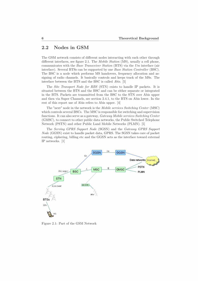
The GSM network consists of different nodes interacting with each other throughdifferent interfaces, see figure 2.1. The Mobile Station (MS), usually a cell phone,communicates with the Base Transceiver Station (BTS) via the Um interface (airinterface). Several BTSs can be supported by one Base Station Controller (BSC).The BSC is a node which performs MS handovers, frequency allocation and as-signing of radio channels. It basically controls and keeps track of the MSs. Theinterface between the BTS and the BSC is called Abis. [5]
The Site Transport Node for RBS (STN) exists to handle IP packets. It issituated between the BTS and the BSC and can be either separate or integratedin the BTS. Packets are transmitted from the BSC to the STN over Abis upperand then via Super Channels, see section 2.4.1, to the BTS on Abis lower. In therest of this report use of Abis refers to Abis upper. [4]
The "next" node in the network is the Mobile services Switching Center (MSC)which controls several BSCs. The MSC is responsible for switching and supervisionfunctions. It can also serve as a gateway, Gateway Mobile services Switching Center(GMSC), to connect to other public data networks, the Public Switched TelephoneNetwork (PSTN) and other Public Land Mobile Networks (PLMN). [5]
The Serving GPRS Support Node (SGSN) and the Gateway GPRS SupportNode (GGSN) exist to handle packet data, GPRS. The SGSN takes care of packetrouting, ciphering, billing etc and the GGSN acts as the interface toward externalIP networks. [1]
Figure 2.1: Part of the GSM Network
2.3 TDMA 7
2.3 TDMA
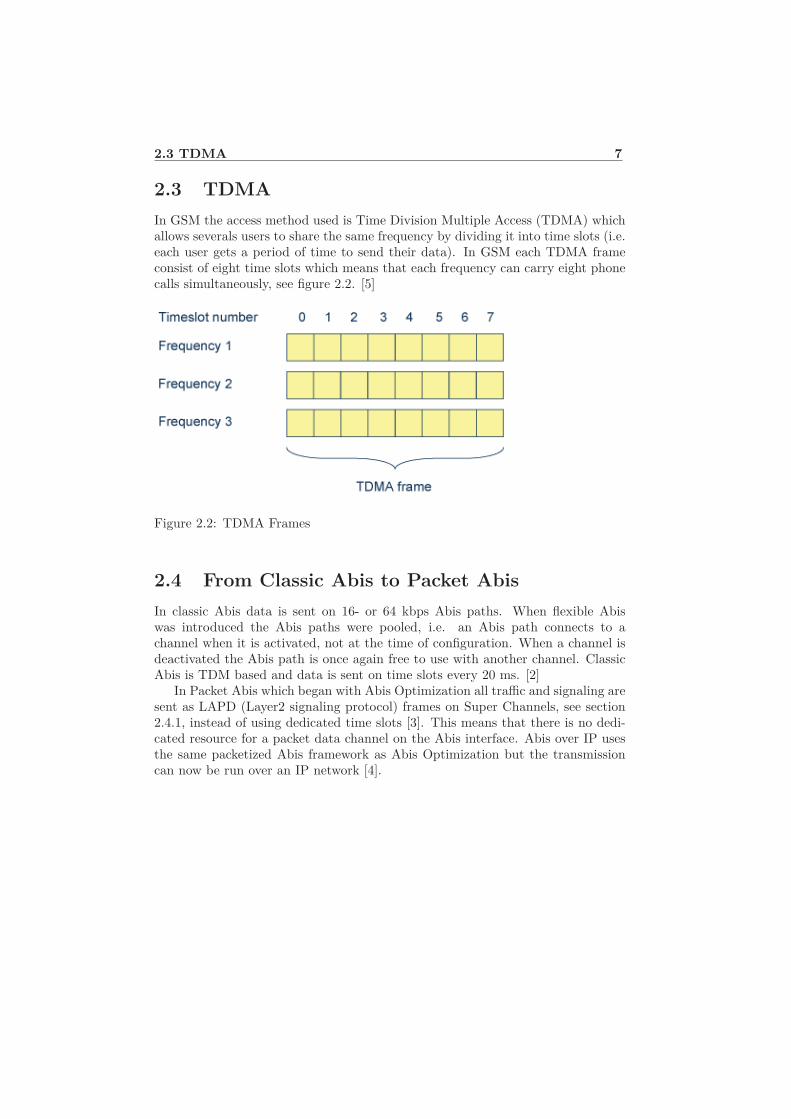
In GSM the access method used is Time Division Multiple Access (TDMA) whichallows severals users to share the same frequency by dividing it into time slots (i.e.each user gets a period of time to send their data). In GSM each TDMA frameconsist of eight time slots which means that each frequency can carry eight phonecalls simultaneously, see figure 2.2. [5]
Figure 2.2: TDMA Frames
2.4 From Classic Abis to Packet Abis
In classic Abis data is sent on 16- or 64 kbps Abis paths. When flexible Abiswas introduced the Abis paths were pooled, i.e. an Abis path connects to achannel when it is activated, not at the time of configuration. When a channel isdeactivated the Abis path is once again free to use with another channel. ClassicAbis is TDM based and data is sent on time slots every 20 ms. [2]
In Packet Abis which began with Abis Optimization all traffic and signaling aresent as LAPD (Layer2 signaling protocol) frames on Super Channels, see section2.4.1, instead of using dedicated time slots [3]. This means that there is no dedi-cated resource for a packet data channel on the Abis interface. Abis over IP usesthe same packetized Abis framework as Abis Optimization but the transmissioncan now be run over an IP network [4].
8 Theoretical Background
2.4.1 Super Channel
One Super Channel is one E1/T1, see 2.4.2, link where 64 kbps consecutive Abistime slots are used as a wideband connection for sending LAPD frames. Thismeans that users share the resources. [4]
2.4.2 E1 and T1
An E1 link has a data rate of 2.048 Mbps and consists of 32 time slots each capableof 64 kbps. T1 signal format carries data at a rate of 1.544 Mbps and can carry 24time slots of 64 kbps. The first byte of each of the 32 respectively 24 time slots aremultiplexed together and the bits are sent one after the other over the channel.The E1 standard is mostly used in Europe and the T1 standard is mostly used inAmerica and Asia. [4]
2.5 Abis Bundling Protocol
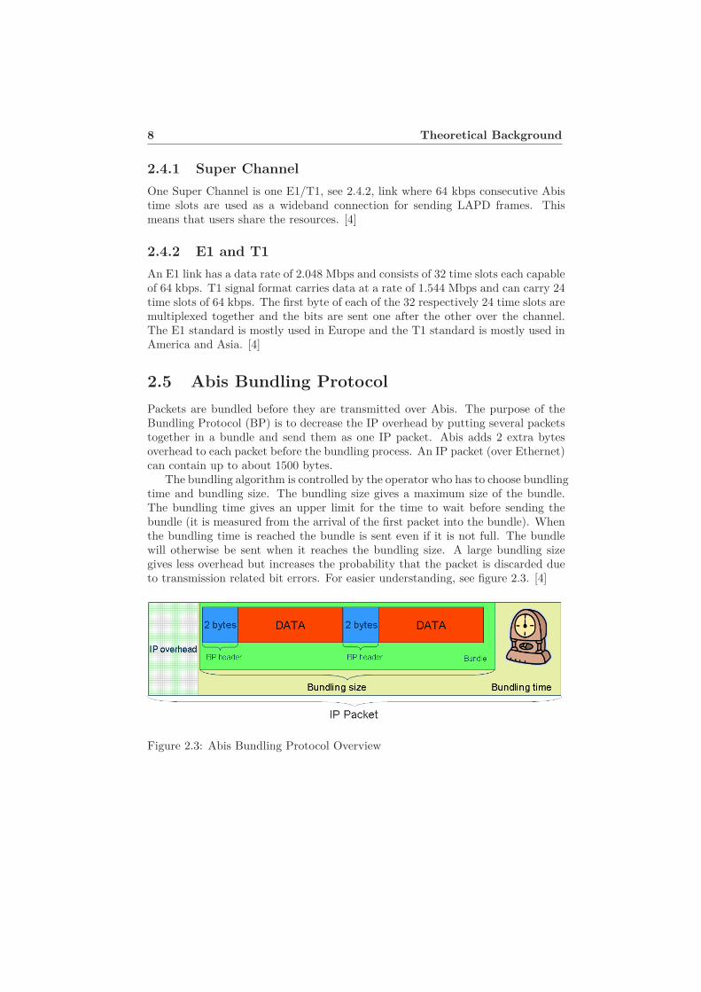
Packets are bundled before they are transmitted over Abis. The purpose of theBundling Protocol (BP) is to decrease the IP overhead by putting several packetstogether in a bundle and send them as one IP packet. Abis adds 2 extra bytesoverhead to each packet before the bundling process. An IP packet (over Ethernet)can contain up to about 1500 bytes.
The bundling algorithm is controlled by the operator who has to choose bundlingtime and bundling size. The bundling size gives a maximum size of the bundle.The bundling time gives an upper limit for the time to wait before sending thebundle (it is measured from the arrival of the first packet into the bundle). Whenthe bundling time is reached the bundle is sent even if it is not full. The bundlewill otherwise be sent when it reaches the bundling size. A large bundling sizegives less overhead but increases the probability that the packet is discarded dueto transmission related bit errors. For easier understanding, see figure 2.3. [4]
Figure 2.3: Abis Bundling Protocol Overview
2.6 Jitter Buffers 9
2.6 Jitter Buffers
Jitter is a typical problem for packet switched networks. Due to the fact thatpackets can be divided and sent separate ways through the network the time foreach packet may vary. Jitter is the variability of the latency over time across anetwork. [7]
To solve this problem jitter buffers are used. A jitter buffer is a buffer thatreceives packets and give them to the receiver at a specific time. If a packet hasnot arrived to the buffer by the time it is supposed to be delivered to the receiver,it will be discarded. [7]
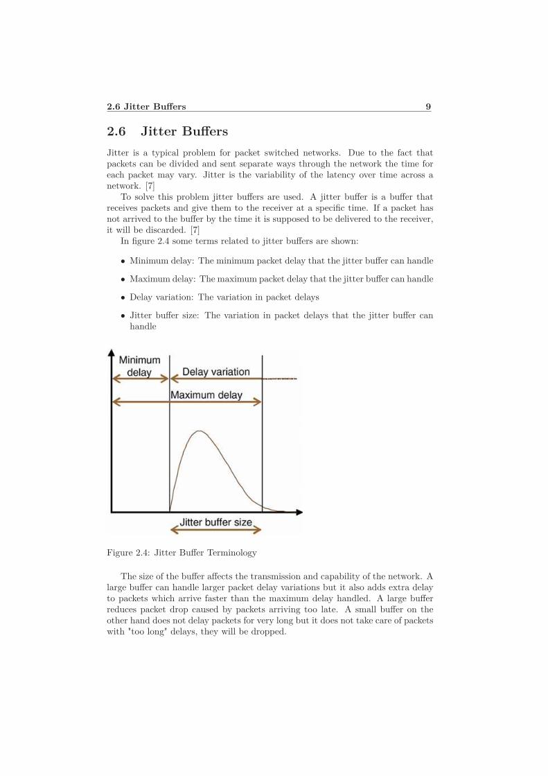
In figure 2.4 some terms related to jitter buffers are shown:
• Minimum delay: The minimum packet delay that the jitter buffer can handle
• Maximum delay: The maximum packet delay that the jitter buffer can handle
• Delay variation: The variation in packet delays
• Jitter buffer size: The variation in packet delays that the jitter buffer canhandle
Figure 2.4: Jitter Buffer Terminology
The size of the buffer affects the transmission and capability of the network. Alarge buffer can handle larger packet delay variations but it also adds extra delayto packets which arrive faster than the maximum delay handled. A large bufferreduces packet drop caused by packets arriving too late. A small buffer on theother hand does not delay packets for very long but it does not take care of packetswith "too long" delays, they will be dropped.
10 Theoretical Background
2.7 P-GSL Timing Advance (PTA)
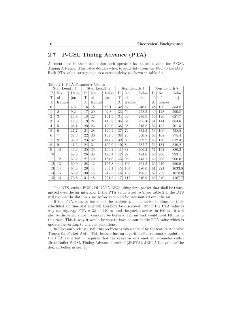
As mentioned in the introduction each operator has to set a value for P-GSLTiming Advance. This value decides when to send data from the BSC to the BTS.Each PTA value corresponds to a certain delay as shown in table 2.1.
Table 2.1: PTA Parameter ValuesStep Length 1 Step Length 2 Step Length 4 Step Length 8
PTA
No.offrames
Delay[ms]
PTA
No.offrames
Delay[ms]
PTA
No.offrames
Delay[ms]
PTA
No.offrames
Delay[ms]
0 1 4.6 16 18 83.1 32 52 240.0 48 120 553.81 2 9.2 17 20 92.3 33 56 258.5 49 128 590.82 3 13.8 18 22 101.5 34 60 276.9 50 136 627.73 4 18.5 19 24 110.8 35 64 295.4 51 144 664.64 5 23.1 20 26 120.0 36 68 313.8 52 152 701.55 6 27.7 21 28 129.2 37 72 332.3 53 160 738.56 7 32.3 22 30 138.5 38 76 350.8 54 168 775.47 8 36.9 23 32 147.7 39 80 369.2 55 176 812.38 9 41.5 24 34 156.9 40 84 387.7 56 184 849.29 10 46.2 25 36 166.2 41 88 406.2 57 192 886.210 11 50.8 26 38 175.4 42 92 424.6 58 200 923.111 12 55.4 27 40 184.6 43 96 443.1 59 208 960.012 13 60.0 28 42 193.8 44 100 461.5 60 216 996.913 14 64.6 29 44 203.1 45 104 480.0 61 224 1033.814 15 69.2 30 46 212.3 46 108 498.5 62 232 1070.815 16 73.8 31 48 221.5 47 112 516.9 63 240 1107.7
The BTS sends a PGSL-DLDATA-REQ asking for a packet that shall be trans-mitted over the air interface. If the PTA value is set to 5, see table 2.1, the BTSwill request the data 27,7 ms before it should be transmitted over the air.
If the PTA value is too small the packets will not arrive in time for theirscheduled air time slot and will therefore be discarded. But if the PTA value isway too big, e.g. PTA = 32 → 240 ms and the packet arrives in 100 ms, it willalso be discarded since it can only be buffered 120 ms and would need 140 ms inthis case. This is why it would be nice to have an automatic PTA value which isupdated according to channel conditions.
In Ericsson’s release, 08B, this problem is taken care of by the feature AdaptiveTimers for Packet Abis. This feature has an algorithm for automatic update ofthe PTA value but it requires that the operator sets another parameter calledJitter Buffer P-GSL Timing Advance downlink (JBPTA). JBPTA is a value of thedesired buffer usage. [4]
Chapter 3
The Abis Model
There are two different aspects to look at to achieve a model for Abis, the protocollayer and the characteristics of the transport. The development of the model isdescribed in the following sections.
3.1 IP Characteristics
A statistical study of delays (Round Trip Times, RTT) is performed to find thecharacteristics of a general IP network. This gives a good model of the behaviorof delays during transmission on Abis.
The statistical study is made through pinging between two computers, i.e.data packets are sent from one computer to the other and then back again. For alldata packets the transaction time, RTT, is measured. It is not possible to controlthe load of the IP network (internet) between the computers but what can becontrolled is the load of the respective connections. A ftp client and server is setup and the pinging is done by the client. The broadband connection of the clientis 100 Mbit downlink and 10 Mbit uplink while the server only has 10 Mbit bothways. The load-variations that is to be tested are:
• No load
• Uplink load (from server to client)
• Downlink load (from client to server)
• Both uplink and downlink load (both directions)
Since load control of the IP network is impossible the pinging takes place atthree different times to see if there are any variations in load/delays over the day.The times to be used are: 04.30, 14.00 and 20.30.
During each ping session 1000 pings with the size 32 bytes are sent to getstatistics that are good enough. It needs to be made sure that the files for up-and download are large enough to last the entire session. Two different intervals
11
12 The Abis Model
between the pings are used to avoid possible repeated irregularities in the network,73 and 100 ms.
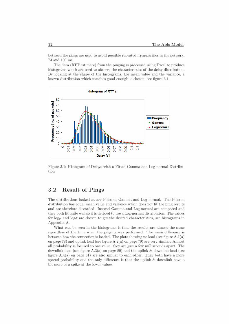
The data (RTT estimate) from the pinging is processed using Excel to producehistograms which are used to observe the characteristics of the delay distribution.By looking at the shape of the histograms, the mean value and the variance, aknown distribution which matches good enough is chosen, see figure 3.1.
Figure 3.1: Histogram of Delays with a Fitted Gamma and Log-normal Distribu-tion
3.2 Result of Pings
The distributions looked at are Poisson, Gamma and Log-normal. The Poissondistribution has equal mean value and variance which does not fit the ping resultsand are therefore discarded. Instead Gamma and Log-normal are compared andthey both fit quite well so it is decided to use a Log-normal distribution. The valuesfor logµ and logσ are chosen to get the desired characteristics, see histograms inAppendix A.
What can be seen in the histograms is that the results are almost the sameregardless of the time when the pinging was performed. The main difference isbetween how the connection is loaded. The plots showing no load (see figure A.1(a)on page 78) and uplink load (see figure A.2(a) on page 79) are very similar. Almostall probability is focused to one value, they are just a few milliseconds apart. Thedownlink load (see figure A.3(a) on page 80) and the uplink & downlink load (seefigure A.4(a) on page 81) are also similar to each other. They both have a morespread probability and the only difference is that the uplink & downlink have abit more of a spike at the lower values.
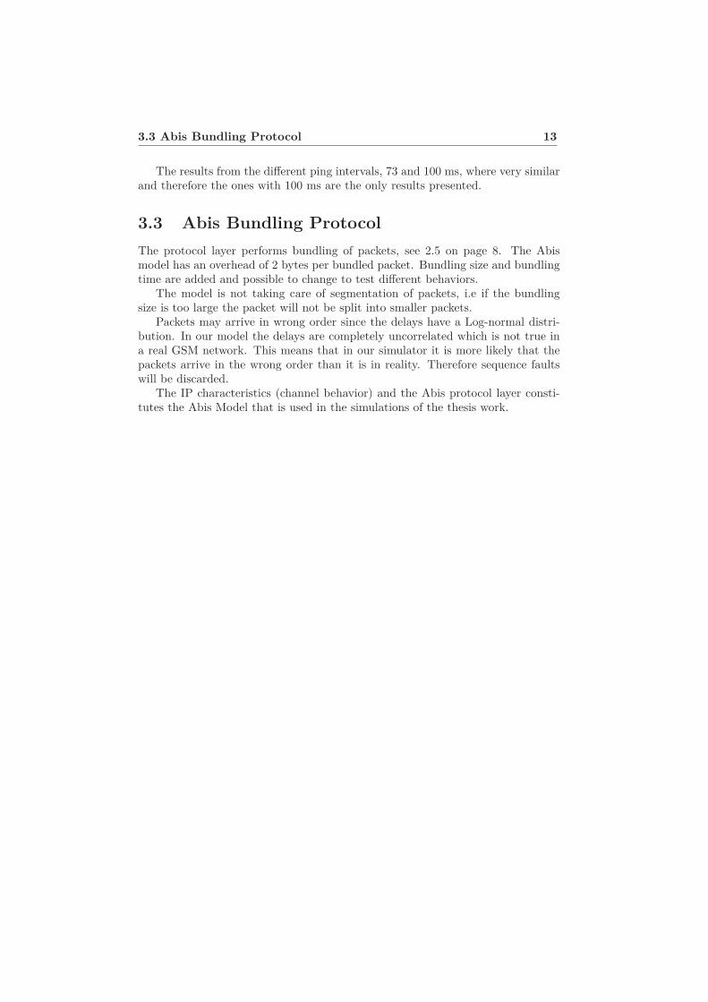
3.3 Abis Bundling Protocol 13
The results from the different ping intervals, 73 and 100 ms, where very similarand therefore the ones with 100 ms are the only results presented.
3.3 Abis Bundling Protocol
The protocol layer performs bundling of packets, see 2.5 on page 8. The Abismodel has an overhead of 2 bytes per bundled packet. Bundling size and bundlingtime are added and possible to change to test different behaviors.
The model is not taking care of segmentation of packets, i.e if the bundlingsize is too large the packet will not be split into smaller packets.
Packets may arrive in wrong order since the delays have a Log-normal distri-bution. In our model the delays are completely uncorrelated which is not true ina real GSM network. This means that in our simulator it is more likely that thepackets arrive in the wrong order than it is in reality. Therefore sequence faultswill be discarded.
The IP characteristics (channel behavior) and the Abis protocol layer consti-tutes the Abis Model that is used in the simulations of the thesis work.

Chapter 4
The Algorithms
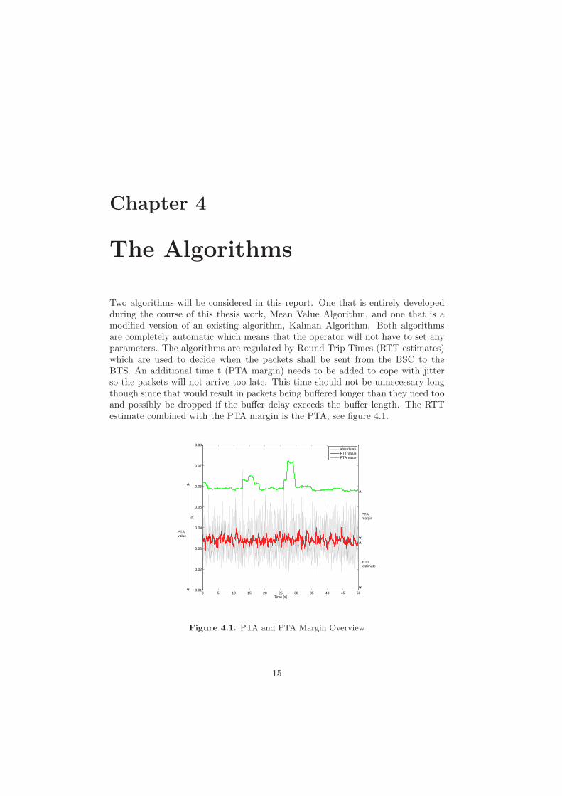
Two algorithms will be considered in this report. One that is entirely developedduring the course of this thesis work, Mean Value Algorithm, and one that is amodified version of an existing algorithm, Kalman Algorithm. Both algorithmsare completely automatic which means that the operator will not have to set anyparameters. The algorithms are regulated by Round Trip Times (RTT estimates)which are used to decide when the packets shall be sent from the BSC to theBTS. An additional time t (PTA margin) needs to be added to cope with jitterso the packets will not arrive too late. This time should not be unnecessary longthough since that would result in packets being buffered longer than they need tooand possibly be dropped if the buffer delay exceeds the buffer length. The RTTestimate combined with the PTA margin is the PTA, see figure 4.1.
0 5 10 15 20 25 30 35 40 45 500.01
0.02
0.03
0.04
0.05
0.06
0.07
0.08
Time [s]
[s]
abis delayRTT valuePTA value
RTTestimate
PTAmargin
PTAvalue
Figure 4.1. PTA and PTA Margin Overview
15
16 The Algorithms
How the RTT part of the newly developed algorithm should work has beendiscussed with experts at Ericsson. When it comes to development of the secondpart of the algorithms, the PTA margin, the approach is as follows. Since thedistribution of the jitter is unknown it is necessary to keep track of how longpackets are being buffered. The statistical study gives a feeling of how the jitterbehaves but it is not certain it always acts the same. At first a few conditionsare stated, basically increasing and decreasing the PTA margin depending on thevariation in buffer delay and the risk of packet loss. By testing the conditions itis realized which extra conditions are needed to accomplish a satisfying behavior.
4.1 Mean Value Algorithm
4.1.1 Overview
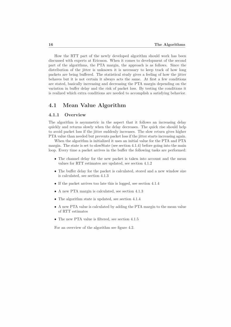
The algorithm is asymmetric in the aspect that it follows an increasing delayquickly and returns slowly when the delay decreases. The quick rise should helpto avoid packet loss if the jitter suddenly increases. The slow return gives higherPTA value than needed but prevents packet loss if the jitter starts increasing again.
When the algorithm is initialized it uses an initial value for the PTA and PTAmargin. The state is set to slowState (see section 4.1.4) before going into the mainloop. Every time a packet arrives in the buffer the following tasks are performed:
• The channel delay for the new packet is taken into account and the meanvalues for RTT estimates are updated, see section 4.1.2
• The buffer delay for the packet is calculated, stored and a new window sizeis calculated, see section 4.1.3
• If the packet arrives too late this is logged, see section 4.1.4
• A new PTA margin is calculated, see section 4.1.3
• The algorithm state is updated, see section 4.1.4
• A new PTA value is calculated by adding the PTA margin to the mean valueof RTT estimates
• The new PTA value is filtered, see section 4.1.5
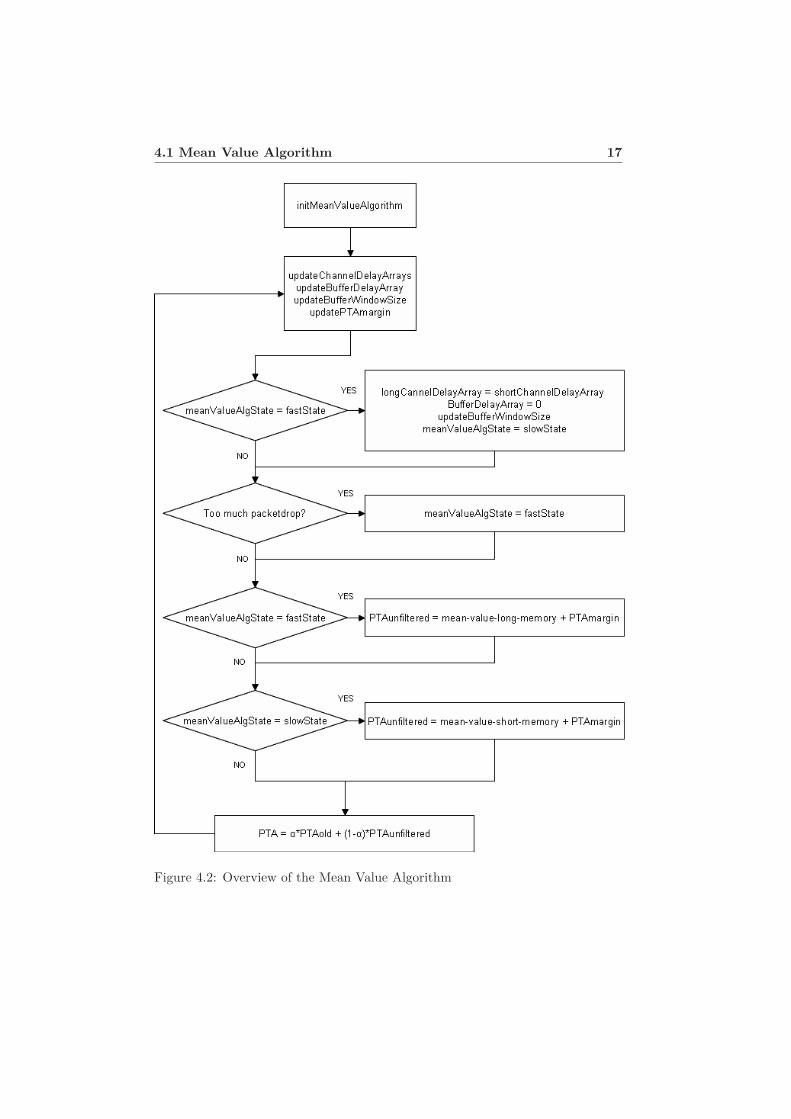
For an overview of the algorithm see figure 4.2.
4.1 Mean Value Algorithm 17
Figure 4.2: Overview of the Mean Value Algorithm
18 The Algorithms
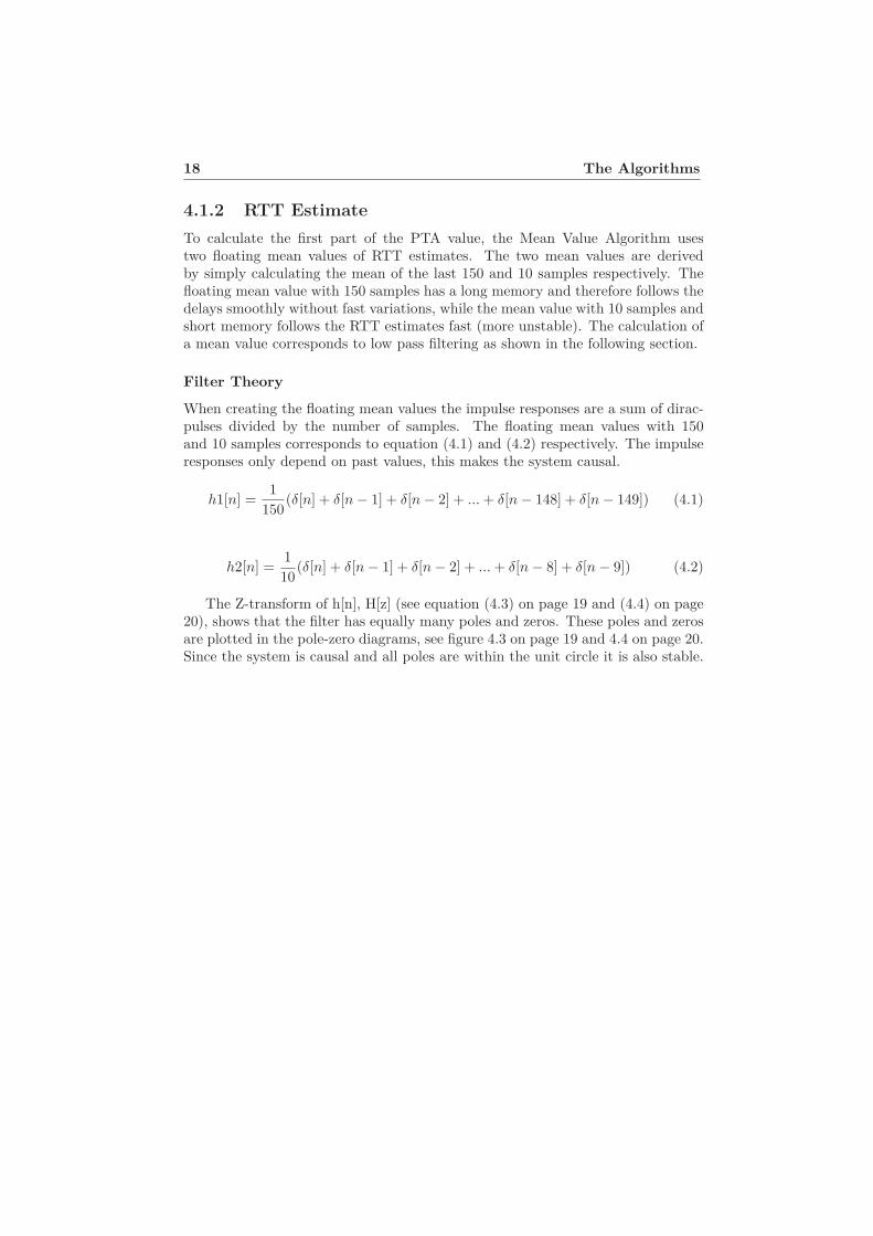
4.1.2 RTT Estimate
To calculate the first part of the PTA value, the Mean Value Algorithm usestwo floating mean values of RTT estimates. The two mean values are derivedby simply calculating the mean of the last 150 and 10 samples respectively. Thefloating mean value with 150 samples has a long memory and therefore follows thedelays smoothly without fast variations, while the mean value with 10 samples andshort memory follows the RTT estimates fast (more unstable). The calculation ofa mean value corresponds to low pass filtering as shown in the following section.
Filter Theory
When creating the floating mean values the impulse responses are a sum of dirac-pulses divided by the number of samples. The floating mean values with 150and 10 samples corresponds to equation (4.1) and (4.2) respectively. The impulseresponses only depend on past values, this makes the system causal.
h1[n] =1
150(δ[n] + δ[n− 1] + δ[n− 2] + ...+ δ[n− 148] + δ[n− 149]) (4.1)
h2[n] =1
10(δ[n] + δ[n− 1] + δ[n− 2] + ...+ δ[n− 8] + δ[n− 9]) (4.2)
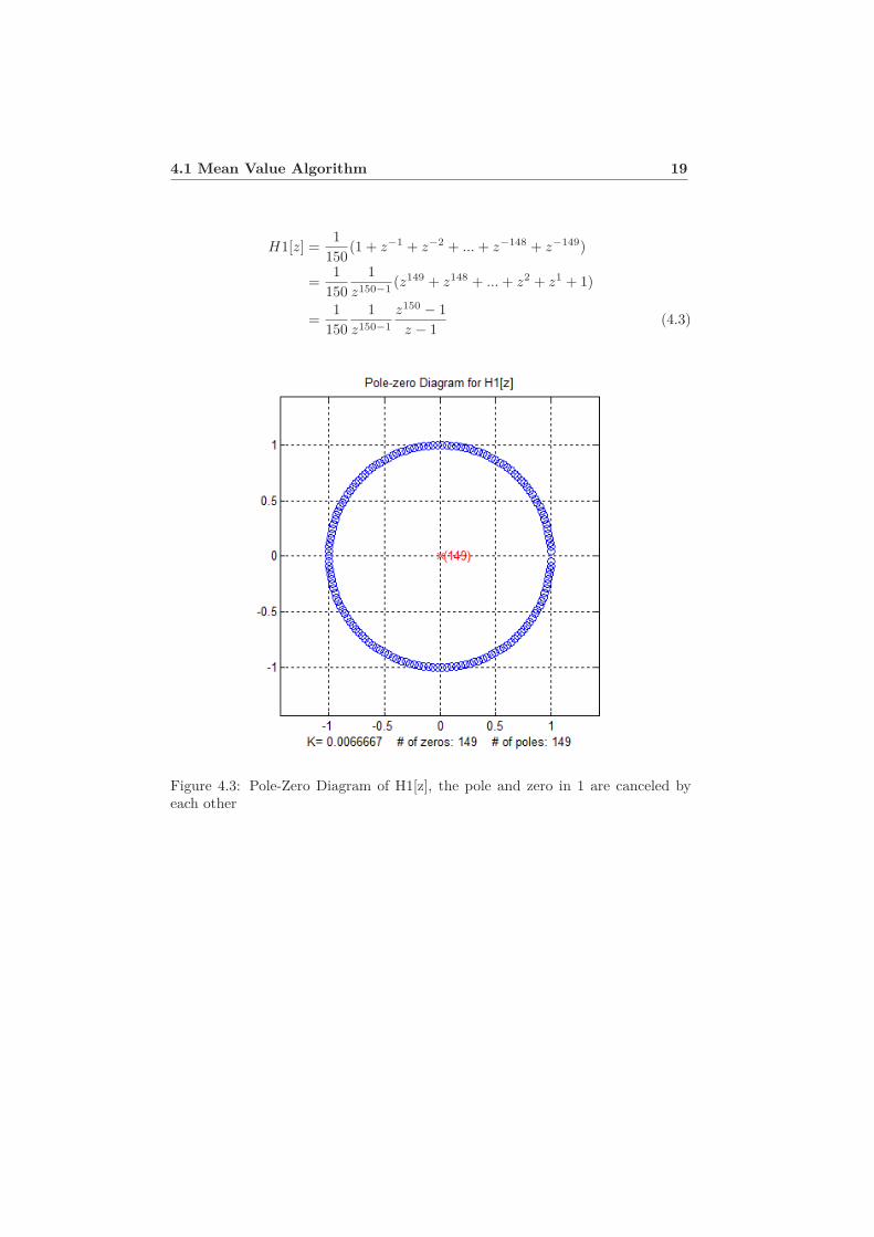
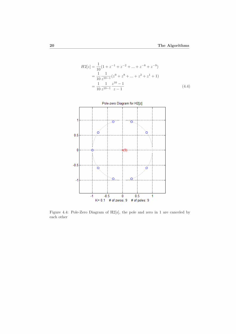
The Z-transform of h[n], H[z] (see equation (4.3) on page 19 and (4.4) on page20), shows that the filter has equally many poles and zeros. These poles and zerosare plotted in the pole-zero diagrams, see figure 4.3 on page 19 and 4.4 on page 20.Since the system is causal and all poles are within the unit circle it is also stable.
4.1 Mean Value Algorithm 19
H1[z] =1
150(1 + z−1 + z−2 + ...+ z−148 + z−149)
=1
150
1
z150−1(z149 + z148 + ...+ z2 + z1 + 1)
=1
150
1
z150−1
z150 − 1
z − 1(4.3)
Figure 4.3: Pole-Zero Diagram of H1[z], the pole and zero in 1 are canceled byeach other
20 The Algorithms
H2[z] =1
10(1 + z−1 + z−2 + ...+ z−8 + z−9)
=1
10
1
z10−1(z9 + z8 + ...+ z2 + z1 + 1)
=1
10
1
z10−1
z10 − 1
z − 1(4.4)
Figure 4.4: Pole-Zero Diagram of H2[z], the pole and zero in 1 are canceled byeach other
4.1 Mean Value Algorithm 21
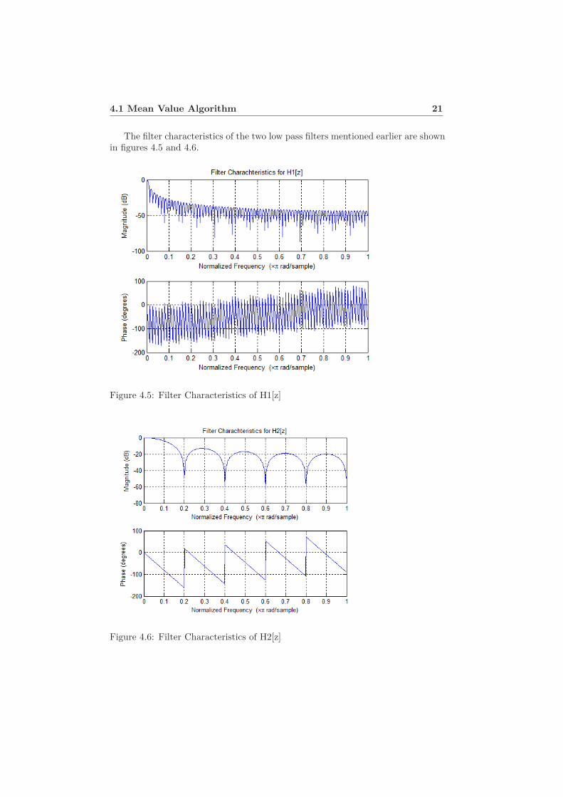
The filter characteristics of the two low pass filters mentioned earlier are shownin figures 4.5 and 4.6.
Figure 4.5: Filter Characteristics of H1[z]
Figure 4.6: Filter Characteristics of H2[z]
22 The Algorithms
4.1.3 PTA Margin
The Mean Value Algorithm changes the PTA margin according to size of the jitterand the buffer usage. The goal is to keep the packets in the buffer as short timeas possible without packet loss.
The last 150 jitter buffer delays are used to calculate a window of buffer delayvariation. The minimum delay is subtracted from the maximum delay to createthe window which gives an indication of how much jitter there is. The windowsize is used when updating the PTA margin.
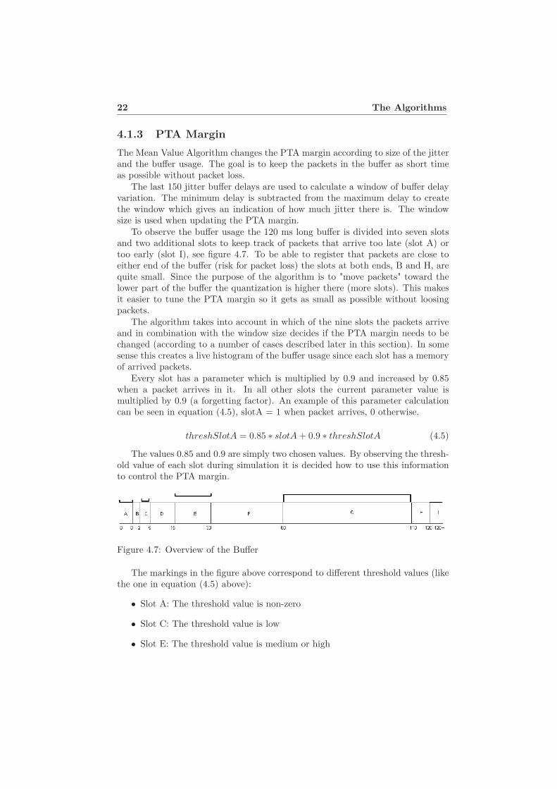
To observe the buffer usage the 120 ms long buffer is divided into seven slotsand two additional slots to keep track of packets that arrive too late (slot A) ortoo early (slot I), see figure 4.7. To be able to register that packets are close toeither end of the buffer (risk for packet loss) the slots at both ends, B and H, arequite small. Since the purpose of the algorithm is to "move packets" toward thelower part of the buffer the quantization is higher there (more slots). This makesit easier to tune the PTA margin so it gets as small as possible without loosingpackets.
The algorithm takes into account in which of the nine slots the packets arriveand in combination with the window size decides if the PTA margin needs to bechanged (according to a number of cases described later in this section). In somesense this creates a live histogram of the buffer usage since each slot has a memoryof arrived packets.
Every slot has a parameter which is multiplied by 0.9 and increased by 0.85when a packet arrives in it. In all other slots the current parameter value ismultiplied by 0.9 (a forgetting factor). An example of this parameter calculationcan be seen in equation (4.5), slotA = 1 when packet arrives, 0 otherwise.
threshSlotA = 0.85 ∗ slotA+ 0.9 ∗ threshSlotA (4.5)
The values 0.85 and 0.9 are simply two chosen values. By observing the thresh-old value of each slot during simulation it is decided how to use this informationto control the PTA margin.
Figure 4.7: Overview of the Buffer
The markings in the figure above correspond to different threshold values (likethe one in equation (4.5) above):
• Slot A: The threshold value is non-zero
• Slot C: The threshold value is low
• Slot E: The threshold value is medium or high
4.1 Mean Value Algorithm 23
• Slot G: The threshold value is smaller than a certain value
• Slot I: The threshold value is zero
Since the threshold value never reaches zero the definition of zero is a reallysmall value (<0.001).
PTA Margin - Cases
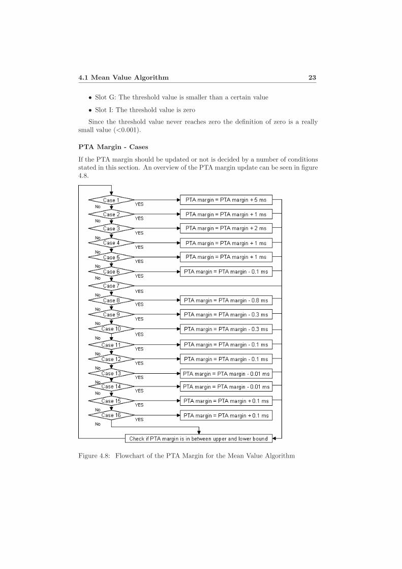
If the PTA margin should be updated or not is decided by a number of conditionsstated in this section. An overview of the PTA margin update can be seen in figure4.8.
Figure 4.8: Flowchart of the PTA Margin for the Mean Value Algorithm
24 The Algorithms
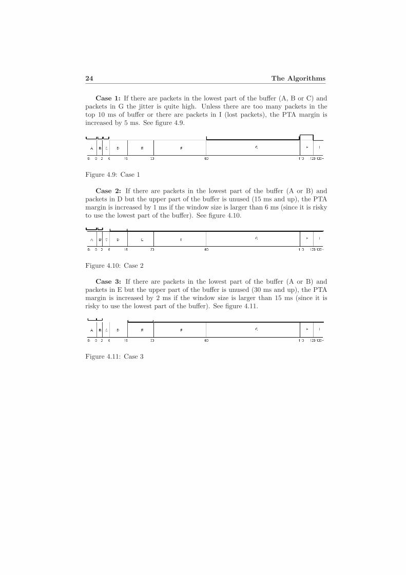
Case 1: If there are packets in the lowest part of the buffer (A, B or C) andpackets in G the jitter is quite high. Unless there are too many packets in thetop 10 ms of buffer or there are packets in I (lost packets), the PTA margin isincreased by 5 ms. See figure 4.9.
Figure 4.9: Case 1
Case 2: If there are packets in the lowest part of the buffer (A or B) andpackets in D but the upper part of the buffer is unused (15 ms and up), the PTAmargin is increased by 1 ms if the window size is larger than 6 ms (since it is riskyto use the lowest part of the buffer). See figure 4.10.
Figure 4.10: Case 2
Case 3: If there are packets in the lowest part of the buffer (A or B) andpackets in E but the upper part of the buffer is unused (30 ms and up), the PTAmargin is increased by 2 ms if the window size is larger than 15 ms (since it isrisky to use the lowest part of the buffer). See figure 4.11.
Figure 4.11: Case 3
4.1 Mean Value Algorithm 25
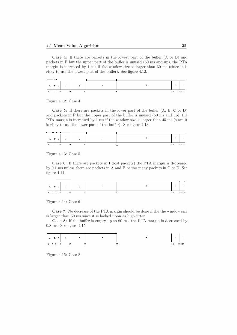
Case 4: If there are packets in the lowest part of the buffer (A or B) andpackets in F but the upper part of the buffer is unused (60 ms and up), the PTAmargin is increased by 1 ms if the window size is larger than 30 ms (since it isrisky to use the lowest part of the buffer). See figure 4.12.
Figure 4.12: Case 4
Case 5: If there are packets in the lower part of the buffer (A, B, C or D)and packets in F but the upper part of the buffer is unused (60 ms and up), thePTA margin is increased by 1 ms if the window size is larger than 45 ms (since itis risky to use the lower part of the buffer). See figure 4.13.
Figure 4.13: Case 5
Case 6: If there are packets in I (lost packets) the PTA margin is decreasedby 0.1 ms unless there are packets in A and B or too many packets in C or D. Seefigure 4.14.
Figure 4.14: Case 6
Case 7: No decrease of the PTA margin should be done if the the window sizeis larger than 50 ms since it is looked upon as high jitter.
Case 8: If the buffer is empty up to 60 ms, the PTA margin is decreased by0.8 ms. See figure 4.15.
Figure 4.15: Case 8
26 The Algorithms
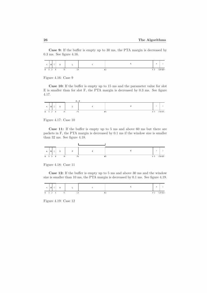
Case 9: If the buffer is empty up to 30 ms, the PTA margin is decreased by0.3 ms. See figure 4.16.
Figure 4.16: Case 9
Case 10: If the buffer is empty up to 15 ms and the parameter value for slotE is smaller than for slot F, the PTA margin is decreased by 0.3 ms. See figure4.17.
Figure 4.17: Case 10
Case 11: If the buffer is empty up to 5 ms and above 60 ms but there arepackets in F, the PTA margin is decreased by 0.1 ms if the window size is smallerthan 32 ms. See figure 4.18.
Figure 4.18: Case 11
Case 12: If the buffer is empty up to 5 ms and above 30 ms and the windowsize is smaller than 10 ms, the PTA margin is decreased by 0.1 ms. See figure 4.19.
Figure 4.19: Case 12
4.1 Mean Value Algorithm 27
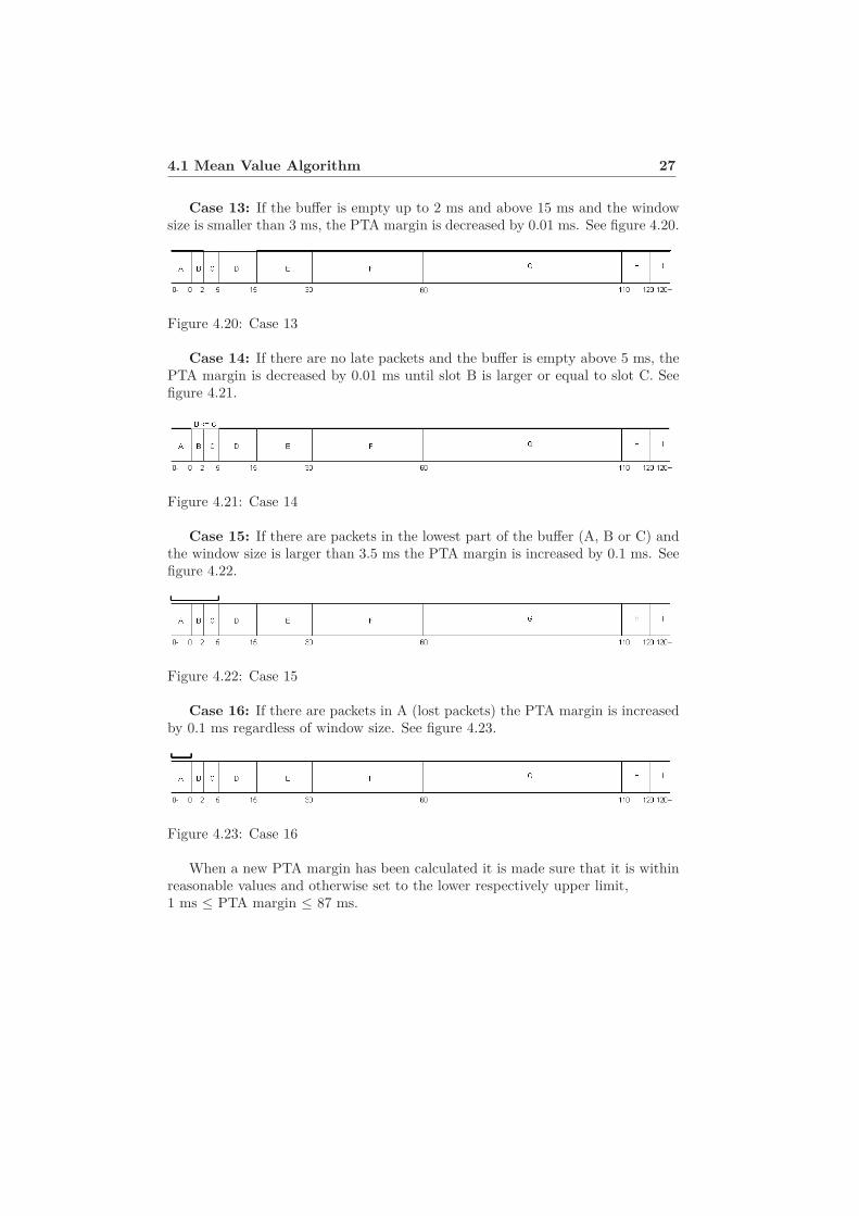
Case 13: If the buffer is empty up to 2 ms and above 15 ms and the windowsize is smaller than 3 ms, the PTA margin is decreased by 0.01 ms. See figure 4.20.
Figure 4.20: Case 13
Case 14: If there are no late packets and the buffer is empty above 5 ms, thePTA margin is decreased by 0.01 ms until slot B is larger or equal to slot C. Seefigure 4.21.
Figure 4.21: Case 14
Case 15: If there are packets in the lowest part of the buffer (A, B or C) andthe window size is larger than 3.5 ms the PTA margin is increased by 0.1 ms. Seefigure 4.22.
Figure 4.22: Case 15
Case 16: If there are packets in A (lost packets) the PTA margin is increasedby 0.1 ms regardless of window size. See figure 4.23.
Figure 4.23: Case 16
When a new PTA margin has been calculated it is made sure that it is withinreasonable values and otherwise set to the lower respectively upper limit,1 ms ≤ PTA margin ≤ 87 ms.
28 The Algorithms
4.1.4 State
The Mean Value Algorithm has two states: slow and fast. Normally the algorithmis in slow state which means that the floating mean value (RTT estimates) withlong memory is used, see section 4.1.2. This keeps the mean value more stablewith slow variations so that delay spikes and dips are ignored. However, if toomany packets are dropped due to late arrival, the algorithm will switch to faststate to become more adaptive and follow the RTT estimates faster. Fast state istriggered when the threshold in equation (4.6) exceeds 1.05, lostpacket = 1 whenpacket is too late, 0 otherwise.
thresholdDroppedPacket = 0.75 ∗ lostPacket+ 0.5 ∗ thresholdDroppedPacket(4.6)
With this equation and threshold value, fast state is triggered after two latepackets. The reason for the "complicated" formula is to have the possibility to tryout different threshold values, for example trigging after: one late packet, thenone packet on time and then another late packet.
When fast state is triggered, the memory of the long-memory-mean-value iserased and replaced with the short-memory-mean-value. Also the stored bufferdelays are erased and a new window size calculated. The state is then set to slowagain but now with no memory of what happened before the fast state triggingoccurred. Since fast state is triggered when packets are too late (increase in delayand/or jitter) but not when they are too early (decrease in delay and/or jitter)the algorithm gets its asymmetric behavior.
4.1.5 PTA Filtering
If the Mean Value Algorithm is in slow state the PTA is calculated by adding themean value with long memory (RTT estimate) and the PTA margin. If it is in faststate on the other hand, the mean value with short memory and the PTA marginare added.
Once the new PTA value is calculated it is filtered to get a more stable PTA(but slower). How much the PTA is filtered is chosen by the parameter α, seeequation (4.7).
PTA = α ∗ PTAold+ (1− α) ∗ PTAunfiltered (4.7)
4.2 Kalman Algorithm 29
4.2 Kalman Algorithm
4.2.1 RTT Estimate
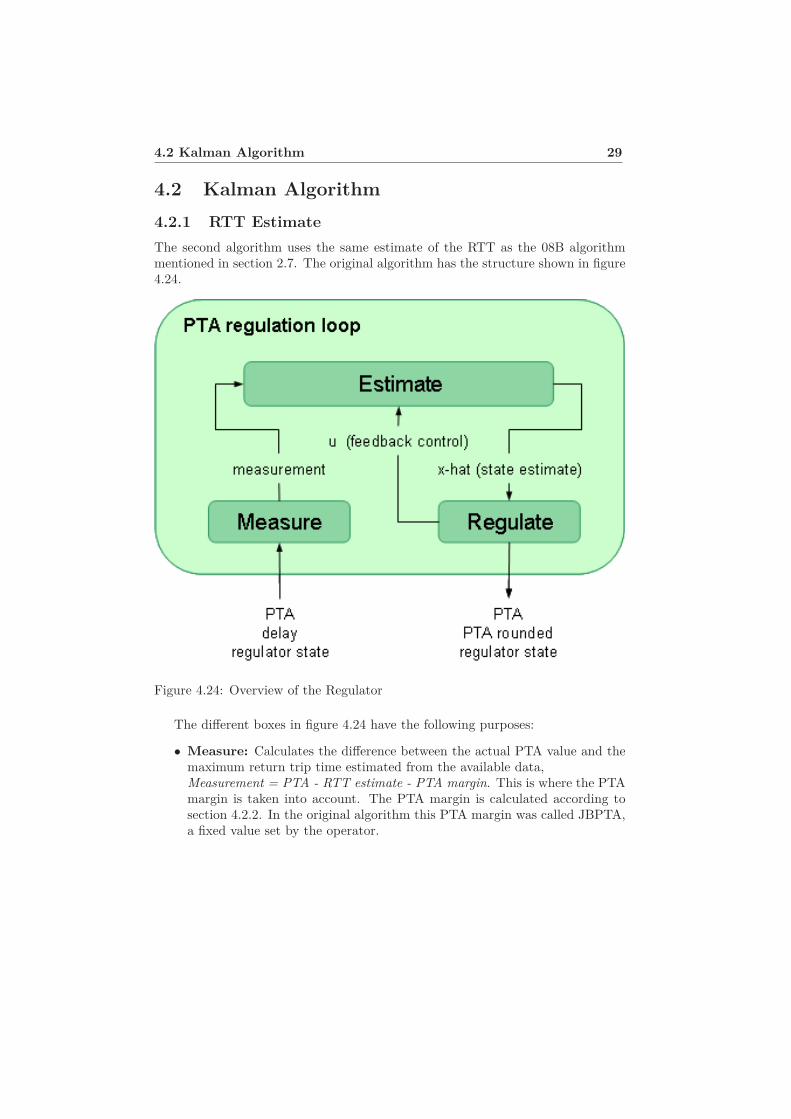
The second algorithm uses the same estimate of the RTT as the 08B algorithmmentioned in section 2.7. The original algorithm has the structure shown in figure4.24.
Figure 4.24: Overview of the Regulator
The different boxes in figure 4.24 have the following purposes:
• Measure: Calculates the difference between the actual PTA value and themaximum return trip time estimated from the available data,Measurement = PTA - RTT estimate - PTA margin. This is where the PTAmargin is taken into account. The PTA margin is calculated according tosection 4.2.2. In the original algorithm this PTA margin was called JBPTA,a fixed value set by the operator.
30 The Algorithms
• Estimate: This box implements an enhanced Kalman observer which worksin two different states. The variance of the measurement and the varianceof the prediction error are calculated. These two variances are then used tochoose state. If either of the two variances are higher than a certain thresholdvalue the algorithm is set to acquisition state. If they are both low enoughit is set to steady state.
• Regulate: The regulate unit implements a linear controller which calculatesthe change in PTA value. The feedback gain is set according to the algorithmstate. When the algorithm is in acquisition state the feedback gain is higherthan when it is in steady state. This makes the algorithm faster when thevariances are high.
For more detailed description of Kalman theory, see [6].
This algorithm is initialized with a PTA value of 4 TDMA frames (≈ 18,46 ms)and it starts in acquisition state to adjust faster.
4.2.2 PTA Margin Estimate
The part of the algorithm that has been developed during this thesis work is theautomatic update of PTA margin estimation. It works the same way as for theMean Value Algorithm except that it is controlled by the mean variance of themeasurement instead of the window size, see section 4.1.3.
PTA Margin - Cases
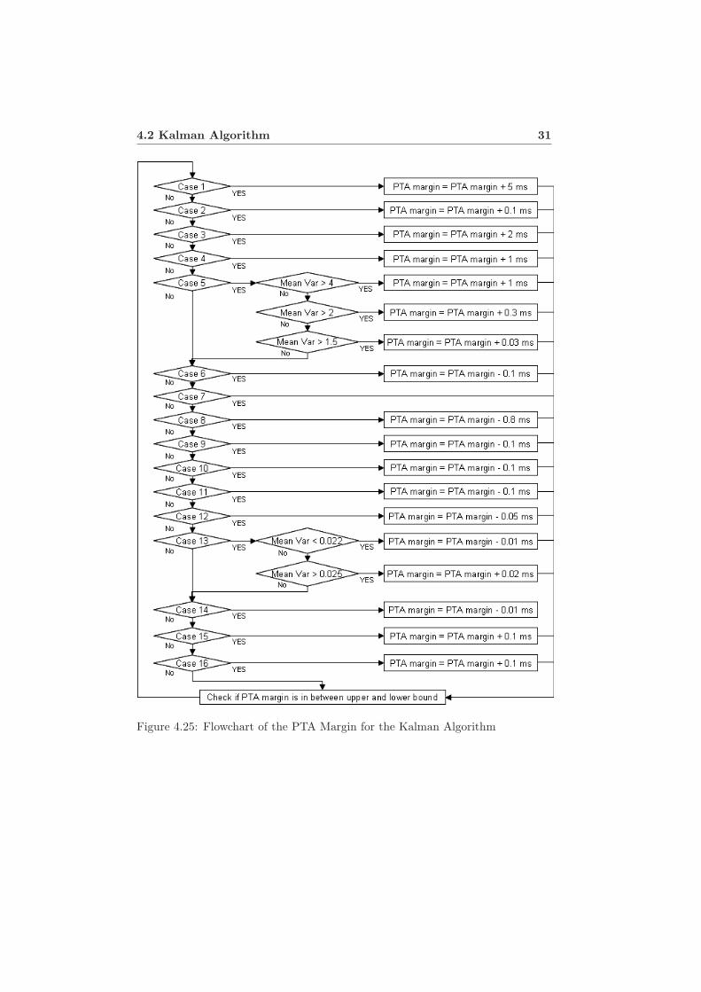
If the PTA margin should be updated or not is decided by a number of conditionsstated in this section. Case 1-16 for both algorithms are equivalent with aspect tobuffer usage, the figures are only repeated for easier reading. An overview of thePTA margin update can be seen in figure 4.25.
4.2 Kalman Algorithm 31
Figure 4.25: Flowchart of the PTA Margin for the Kalman Algorithm
32 The Algorithms
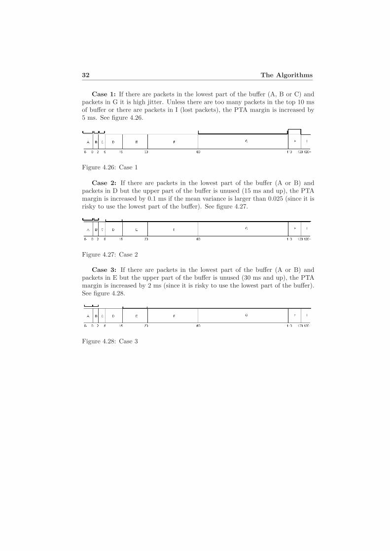
Case 1: If there are packets in the lowest part of the buffer (A, B or C) andpackets in G it is high jitter. Unless there are too many packets in the top 10 msof buffer or there are packets in I (lost packets), the PTA margin is increased by5 ms. See figure 4.26.
Figure 4.26: Case 1
Case 2: If there are packets in the lowest part of the buffer (A or B) andpackets in D but the upper part of the buffer is unused (15 ms and up), the PTAmargin is increased by 0.1 ms if the mean variance is larger than 0.025 (since it isrisky to use the lowest part of the buffer). See figure 4.27.
Figure 4.27: Case 2
Case 3: If there are packets in the lowest part of the buffer (A or B) andpackets in E but the upper part of the buffer is unused (30 ms and up), the PTAmargin is increased by 2 ms (since it is risky to use the lowest part of the buffer).See figure 4.28.
Figure 4.28: Case 3
4.2 Kalman Algorithm 33
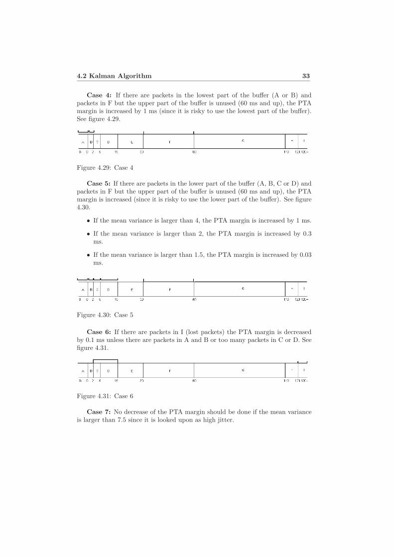
Case 4: If there are packets in the lowest part of the buffer (A or B) andpackets in F but the upper part of the buffer is unused (60 ms and up), the PTAmargin is increased by 1 ms (since it is risky to use the lowest part of the buffer).See figure 4.29.
Figure 4.29: Case 4
Case 5: If there are packets in the lower part of the buffer (A, B, C or D) andpackets in F but the upper part of the buffer is unused (60 ms and up), the PTAmargin is increased (since it is risky to use the lower part of the buffer). See figure4.30.
• If the mean variance is larger than 4, the PTA margin is increased by 1 ms.
• If the mean variance is larger than 2, the PTA margin is increased by 0.3ms.
• If the mean variance is larger than 1.5, the PTA margin is increased by 0.03ms.
Figure 4.30: Case 5
Case 6: If there are packets in I (lost packets) the PTA margin is decreasedby 0.1 ms unless there are packets in A and B or too many packets in C or D. Seefigure 4.31.
Figure 4.31: Case 6
Case 7: No decrease of the PTA margin should be done if the mean varianceis larger than 7.5 since it is looked upon as high jitter.
34 The Algorithms
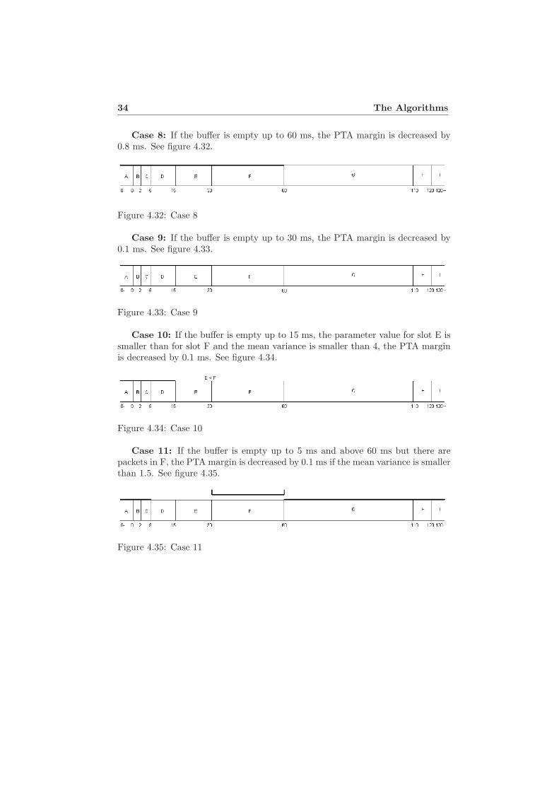
Case 8: If the buffer is empty up to 60 ms, the PTA margin is decreased by0.8 ms. See figure 4.32.
Figure 4.32: Case 8
Case 9: If the buffer is empty up to 30 ms, the PTA margin is decreased by0.1 ms. See figure 4.33.
Figure 4.33: Case 9
Case 10: If the buffer is empty up to 15 ms, the parameter value for slot E issmaller than for slot F and the mean variance is smaller than 4, the PTA marginis decreased by 0.1 ms. See figure 4.34.
Figure 4.34: Case 10
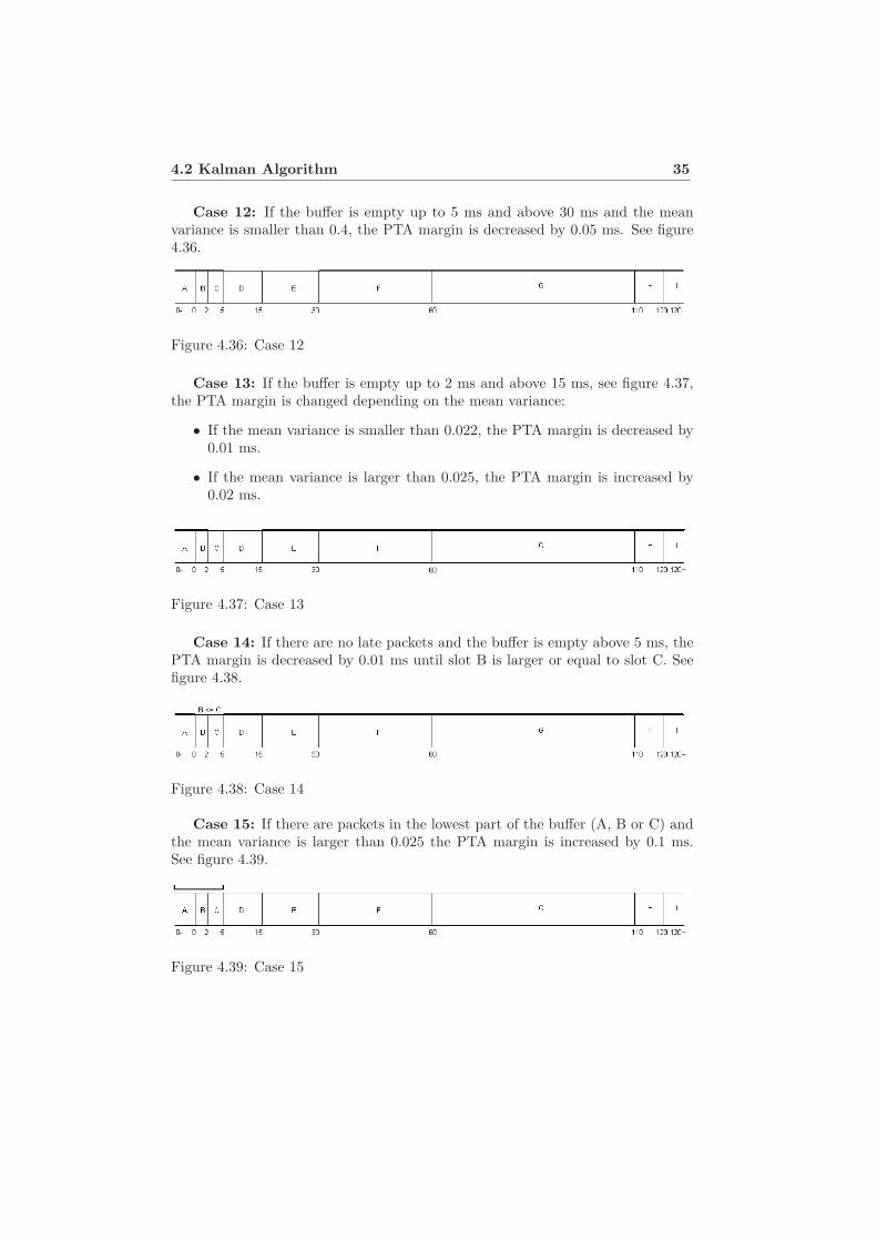
Case 11: If the buffer is empty up to 5 ms and above 60 ms but there arepackets in F, the PTA margin is decreased by 0.1 ms if the mean variance is smallerthan 1.5. See figure 4.35.
Figure 4.35: Case 11
4.2 Kalman Algorithm 35
Case 12: If the buffer is empty up to 5 ms and above 30 ms and the meanvariance is smaller than 0.4, the PTA margin is decreased by 0.05 ms. See figure4.36.
Figure 4.36: Case 12
Case 13: If the buffer is empty up to 2 ms and above 15 ms, see figure 4.37,the PTA margin is changed depending on the mean variance:
• If the mean variance is smaller than 0.022, the PTA margin is decreased by0.01 ms.
• If the mean variance is larger than 0.025, the PTA margin is increased by0.02 ms.
Figure 4.37: Case 13
Case 14: If there are no late packets and the buffer is empty above 5 ms, thePTA margin is decreased by 0.01 ms until slot B is larger or equal to slot C. Seefigure 4.38.
Figure 4.38: Case 14
Case 15: If there are packets in the lowest part of the buffer (A, B or C) andthe mean variance is larger than 0.025 the PTA margin is increased by 0.1 ms.See figure 4.39.
Figure 4.39: Case 15
36 The Algorithms
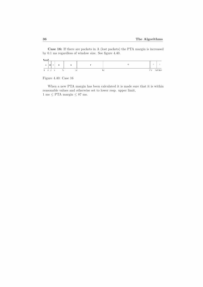
Case 16: If there are packets in A (lost packets) the PTA margin is increasedby 0.1 ms regardless of window size. See figure 4.40.
Figure 4.40: Case 16
When a new PTA margin has been calculated it is made sure that it is withinreasonable values and otherwise set to lower resp. upper limit,1 ms ≤ PTA margin ≤ 87 ms.
Chapter 5
The Simulator
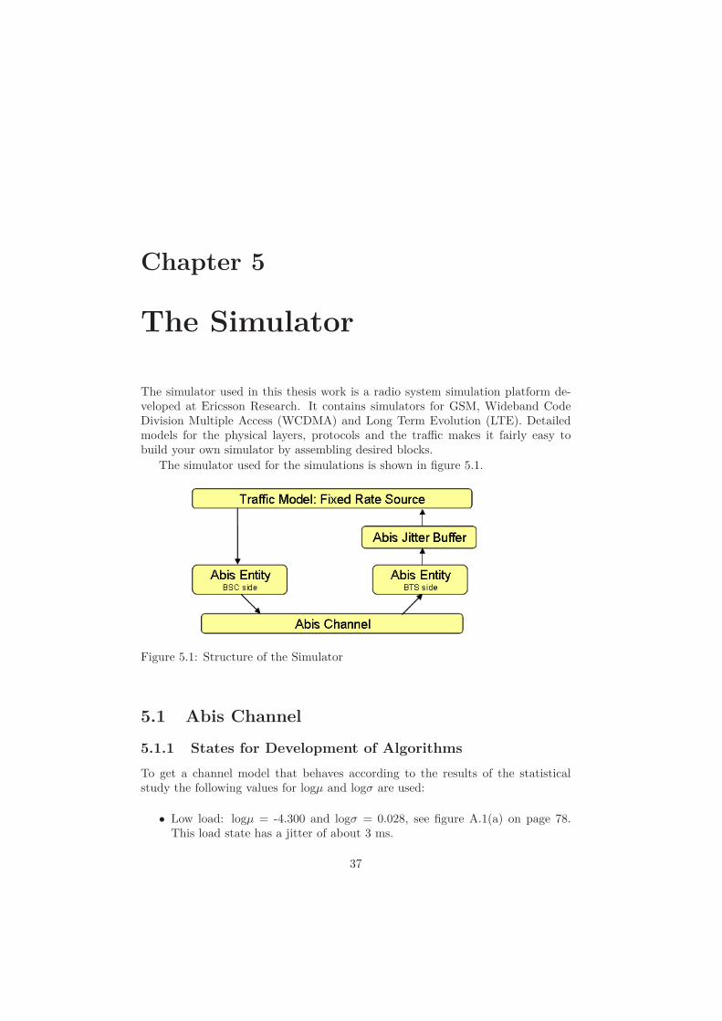
The simulator used in this thesis work is a radio system simulation platform de-veloped at Ericsson Research. It contains simulators for GSM, Wideband CodeDivision Multiple Access (WCDMA) and Long Term Evolution (LTE). Detailedmodels for the physical layers, protocols and the traffic makes it fairly easy tobuild your own simulator by assembling desired blocks.
The simulator used for the simulations is shown in figure 5.1.
Figure 5.1: Structure of the Simulator
5.1 Abis Channel
5.1.1 States for Development of Algorithms
To get a channel model that behaves according to the results of the statisticalstudy the following values for logµ and logσ are used:
• Low load: logµ = -4.300 and logσ = 0.028, see figure A.1(a) on page 78.This load state has a jitter of about 3 ms.
37
38 The Simulator
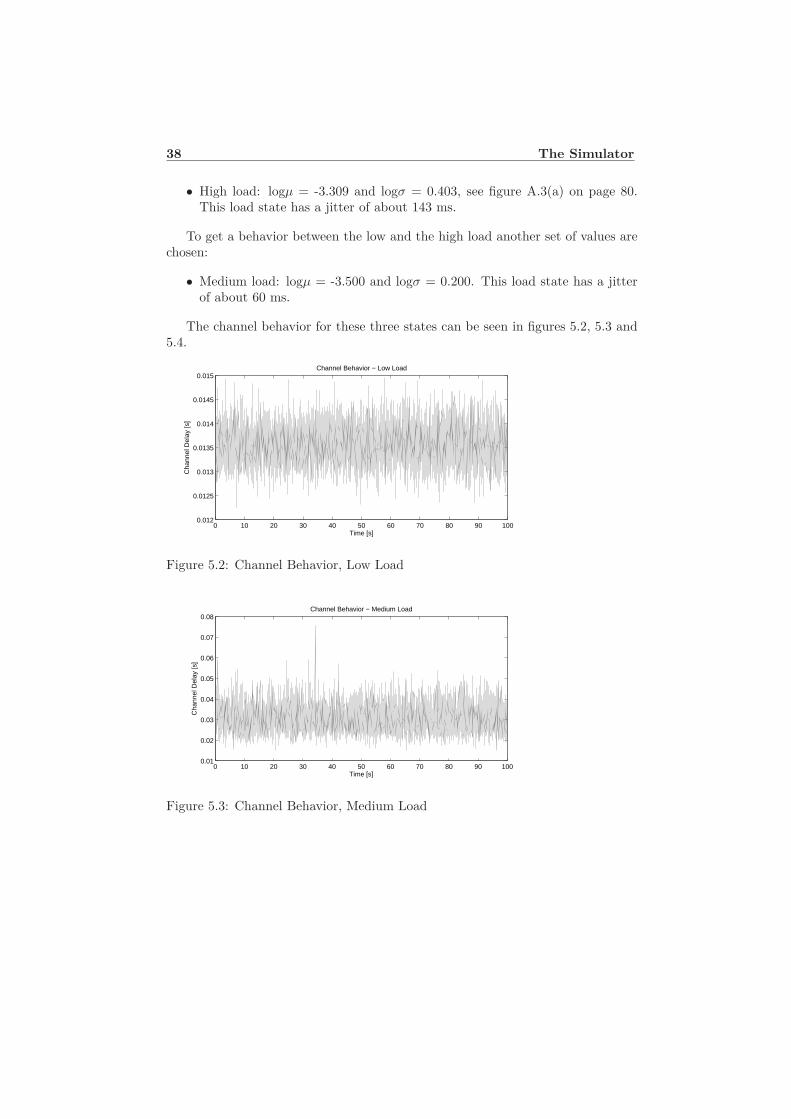
• High load: logµ = -3.309 and logσ = 0.403, see figure A.3(a) on page 80.This load state has a jitter of about 143 ms.
To get a behavior between the low and the high load another set of values arechosen:
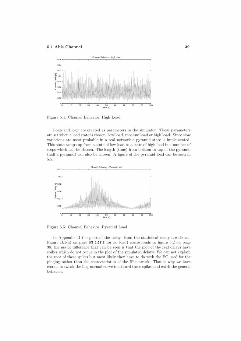
• Medium load: logµ = -3.500 and logσ = 0.200. This load state has a jitterof about 60 ms.
The channel behavior for these three states can be seen in figures 5.2, 5.3 and5.4.
0 10 20 30 40 50 60 70 80 90 1000.012
0.0125
0.013
0.0135
0.014
0.0145
0.015
Time [s]
Cha
nnel
Del
ay [s
]
Channel Behavior − Low Load
Figure 5.2: Channel Behavior, Low Load
0 10 20 30 40 50 60 70 80 90 1000.01
0.02
0.03
0.04
0.05
0.06
0.07
0.08
Time [s]
Cha
nnel
Del
ay [s
]
Channel Behavior − Medium Load
Figure 5.3: Channel Behavior, Medium Load
5.1 Abis Channel 39
0 10 20 30 40 50 60 70 80 90 1000
0.02
0.04
0.06
0.08
0.1
0.12
0.14
0.16
Time [s]
Cha
nnel
Del
ay [s
]Channel Behavior − High Load
Figure 5.4: Channel Behavior, High Load
Logµ and logσ are created as parameters in the simulator. These parametersare set when a load state is chosen: lowLoad, mediumLoad or highLoad. Since slowvariations are most probable in a real network a pyramid state is implemented.This state ramps up from a state of low load to a state of high load in a number ofsteps which can be chosen. The length (time) from bottom to top of the pyramid(half a pyramid) can also be chosen. A figure of the pyramid load can be seen in5.5.
0 10 20 30 40 50 60 70 80 90 1000
0.02
0.04
0.06
0.08
0.1
0.12
Time [s]
Cha
nnel
Del
ay [s
]
Channel Behavior − Pyramid Load
Figure 5.5: Channel Behavior, Pyramid Load
In Appendix B the plots of the delays from the statistical study are shown.Figure B.1(a) on page 83 (RTT for no load) corresponds to figure 5.2 on page38, the major difference that can be seen is that the plot of the real delays havespikes which do not occur in the plot of the simulated delays. We can not explainthe root of these spikes but most likely they have to do with the PC used for thepinging rather than the characteristics of the IP network. That is why we havechosen to tweak the Log-normal curve to discard these spikes and catch the generalbehavior.
40 The Simulator
5.1.2 States for Validation of Algorithms
Once the algorithms have been developed using the states mentioned in the previ-ous section, new states are implemented to be able to test the performance of thealgorithms.
The new states are:
• Low load 2: Little more jitter than low load, approximately 12 ms.
• Low-medium load: Jitter between low and medium load, approximately 42ms.
• Medium load 2: A little more jitter than medium load, approximately 73ms.
• Medium-high load: Jitter between medium and high load, approximately124 ms.
• High load 2: Higher jitter than high load, approximately 394 ms (more thanthe buffer can handle).
• Random load: Changes between low, medium and high load after a certaintime t chosen by a parameter, see figures 6.19 and 6.20 on page 48
• A step function is implemented mainly to test the RTT parts of the algo-rithms, see section 6.2.2
5.2 Abis Protocol
In the Abis Entity which takes care of the Bundling Protocol aspects, see section2.5, bundling time and bundling size are added as parameters and the functionalityis implemented. The abis overhead is also implemented.
5.3 Jitter Buffer 41
5.3 Jitter Buffer
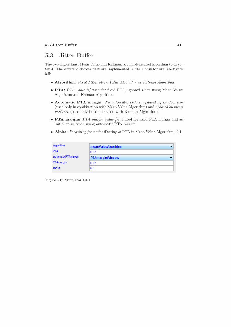
The two algorithms, Mean Value and Kalman, are implemented according to chap-ter 4. The different choices that are implemented in the simulator are, see figure5.6:
• Algorithm: Fixed PTA, Mean Value Algorithm or Kalman Algorithm
• PTA: PTA value [s] used for fixed PTA, ignored when using Mean ValueAlgorithm and Kalman Algorithm
• Automatic PTA margin: No automatic update, updated by window size(used only in combination with Mean Value Algorithm) and updated by meanvariance (used only in combination with Kalman Algorithm)
• PTA margin: PTA margin value [s] is used for fixed PTA margin and asinitial value when using automatic PTA margin
• Alpha: Forgetting factor for filtering of PTA in Mean Value Algorithm, [0,1]
Figure 5.6: Simulator GUI

Chapter 6
Algorithm Behavior
To see some behaviors of the algorithms a few plots of channel delays and PTAvalues are shown in this chapter. Different channel delays have been used, bothsimulation and validation data, see section 5.1. Unless otherwise noted all simu-lations are run using automatic PTA margin.
6.1 Simulation Data
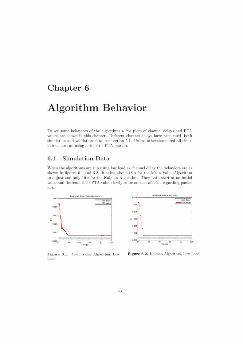
When the algorithms are run using low load as channel delay the behaviors are asshown in figures 6.1 and 6.2. It takes about 18 s for the Mean Value Algorithmto adjust and only 10 s for the Kalman Algorithm. They both start at an initialvalue and decrease their PTA value slowly to be on the safe side regarding packetloss.
0 20 40 60 80 1000.015
0.02
0.025
0.03
0.035
0.04
Time [s]
[s]
Low Load, Mean Value Algorithm
abis delayPTA value
Figure 6.1. Mean Value Algorithm, Low
Load
0 20 40 60 80 1000.015
0.02
0.025
0.03
0.035
0.04
0.045
Time [s]
[s]
Low Load, Kalman Algorithm
abis delayPTA value
Figure 6.2. Kalman Algorithm, Low Load
43
44 Algorithm Behavior
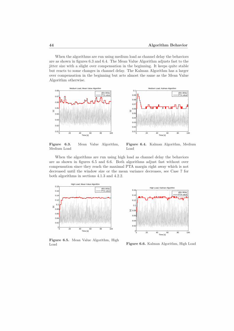
When the algorithms are run using medium load as channel delay the behaviorsare as shown in figures 6.3 and 6.4. The Mean Value Algorithm adjusts fast to thejitter size with a slight over compensation in the beginning. It keeps quite stablebut reacts to some changes in channel delay. The Kalman Algorithm has a largerover compensation in the beginning but acts almost the same as the Mean ValueAlgorithm otherwise.
0 20 40 60 80 1000.01
0.02
0.03
0.04
0.05
0.06
0.07
0.08
Time [s]
[s]
Medium Load, Mean Value Algorithm
abis delayPTA value
Figure 6.3. Mean Value Algorithm,
Medium Load
0 20 40 60 80 1000.01
0.02
0.03
0.04
0.05
0.06
0.07
0.08
0.09
0.1
Time [s]
[s]
Medium Load, Kalman Algorithm
abis delayPTA value
Figure 6.4. Kalman Algorithm, Medium
Load
When the algorithms are run using high load as channel delay the behaviorsare as shown in figures 6.5 and 6.6. Both algorithms adjust fast without overcompensation since they reach the maximal PTA margin right away which is notdecreased until the window size or the mean variance decreases, see Case 7 forboth algorithms in sections 4.1.3 and 4.2.2.
0 20 40 60 80 1000
0.02
0.04
0.06
0.08
0.1
0.12
0.14
0.16
0.18
Time [s]
[s]
High Load, Mean Value Algorithm
abis delayPTA value
Figure 6.5. Mean Value Algorithm, High
Load
0 20 40 60 80 1000
0.02
0.04
0.06
0.08
0.1
0.12
0.14
0.16
Time [s]
[s]
High Load, Kalman Algorithm
abis delayPTA value
Figure 6.6. Kalman Algorithm, High Load
6.1 Simulation Data 45
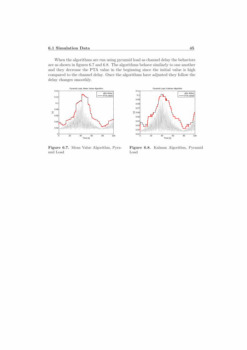
When the algorithms are run using pyramid load as channel delay the behaviorsare as shown in figures 6.7 and 6.8. The algorithms behave similarly to one anotherand they decrease the PTA value in the beginning since the initial value is highcompared to the channel delay. Once the algorithms have adjusted they follow thedelay changes smoothly.
0 20 40 60 80 1000
0.02
0.04
0.06
0.08
0.1
0.12
0.14
Time [s]
[s]
Pyramid Load, Mean Value Algorithm
abis delayPTA value
Figure 6.7. Mean Value Algorithm, Pyra-
mid Load
0 20 40 60 80 1000.01
0.02
0.03
0.04
0.05
0.06
0.07
0.08
0.09
0.1
0.11
Time [s]
[s]
Pyramid Load, Kalman Algorithm
abis delayPTA value
Figure 6.8. Kalman Algorithm, Pyramid
Load
46 Algorithm Behavior
6.2 Validation Data
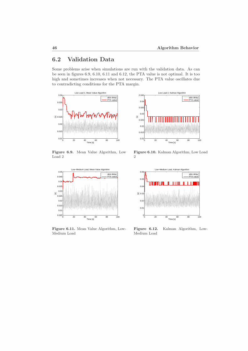
Some problems arise when simulations are run with the validation data. As canbe seen in figures 6.9, 6.10, 6.11 and 6.12, the PTA value is not optimal. It is toohigh and sometimes increases when not necessary. The PTA value oscillates dueto contradicting conditions for the PTA margin.
0 20 40 60 80 1000.01
0.015
0.02
0.025
0.03
0.035
0.04
Time [s]
[s]
Low Load 2, Mean Value Algorithm
abis delayPTA value
Figure 6.9. Mean Value Algorithm, Low
Load 2
0 20 40 60 80 1000.01
0.015
0.02
0.025
0.03
0.035
0.04
0.045
Time [s]
[s]
Low Load 2, Kalman Algorithm
abis delayPTA value
Figure 6.10. Kalman Algorithm, Low Load
2
0 20 40 60 80 1000.005
0.01
0.015
0.02
0.025
0.03
0.035
0.04
0.045
0.05
Time [s]
[s]
Low−Medium Load, Mean Value Algorithm
abis delayPTA value
Figure 6.11. Mean Value Algorithm, Low-
Medium Load
0 20 40 60 80 1000
0.01
0.02
0.03
0.04
0.05
0.06
Time [s]
[s]
Low−Medium Load, Kalman Algorithm
abis delayPTA value
Figure 6.12. Kalman Algorithm, Low-
Medium Load
6.2 Validation Data 47
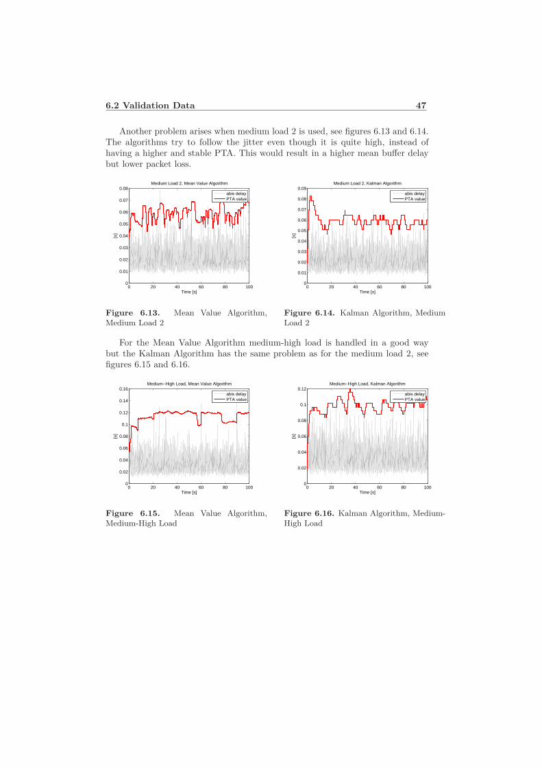
Another problem arises when medium load 2 is used, see figures 6.13 and 6.14.The algorithms try to follow the jitter even though it is quite high, instead ofhaving a higher and stable PTA. This would result in a higher mean buffer delaybut lower packet loss.
0 20 40 60 80 1000
0.01
0.02
0.03
0.04
0.05
0.06
0.07
0.08
Time [s]
[s]
Medium Load 2, Mean Value Algorithm
abis delayPTA value
Figure 6.13. Mean Value Algorithm,
Medium Load 2
0 20 40 60 80 1000
0.01
0.02
0.03
0.04
0.05
0.06
0.07
0.08
0.09
Time [s][s
]
Medium Load 2, Kalman Algorithm
abis delayPTA value
Figure 6.14. Kalman Algorithm, Medium
Load 2
For the Mean Value Algorithm medium-high load is handled in a good waybut the Kalman Algorithm has the same problem as for the medium load 2, seefigures 6.15 and 6.16.
0 20 40 60 80 1000
0.02
0.04
0.06
0.08
0.1
0.12
0.14
0.16
Time [s]
[s]
Medium−High Load, Mean Value Algorithm
abis delayPTA value
Figure 6.15. Mean Value Algorithm,
Medium-High Load
0 20 40 60 80 1000
0.02
0.04
0.06
0.08
0.1
0.12
Time [s]
[s]
Medium−High Load, Kalman Algorithm
abis delayPTA value
Figure 6.16. Kalman Algorithm, Medium-
High Load
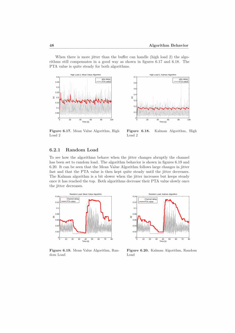
48 Algorithm Behavior
When there is more jitter than the buffer can handle (high load 2) the algo-rithms still compensates in a good way as shown in figures 6.17 and 6.18. ThePTA value is quite steady for both algorithms.
0 20 40 60 80 1000
0.05
0.1
0.15
0.2
0.25
0.3
0.35
0.4
Time [s]
[s]
High Load 2, Mean Value Algorithm
abis delayPTA value
Figure 6.17. Mean Value Algorithm, High
Load 2
0 20 40 60 80 1000
0.1
0.2
0.3
0.4
0.5
0.6
0.7
Time [s]
[s]
High Load 2, Kalman Algorithm
abis delayPTA value
Figure 6.18. Kalman Algorithm, High
Load 2
6.2.1 Random Load
To see how the algorithms behave when the jitter changes abruptly the channelhas been set to random load. The algorithm behavior is shown in figures 6.19 and6.20. It can be seen that the Mean Value Algorithm follows large changes in jitterfast and that the PTA value is then kept quite steady until the jitter decreases.The Kalman algorithm is a bit slower when the jitter increases but keeps steadyonce it has reached the top. Both algorithms decrease their PTA value slowly oncethe jitter decreases.
0 10 20 30 40 50 60 70 800
0.02
0.04
0.06
0.08
0.1
0.12
0.14
Time [s]
[s]
Random Load, Mean Value Algorithm
Channel delayPTA value
Figure 6.19. Mean Value Algorithm, Ran-
dom Load
0 10 20 30 40 50 60 70 800
0.02
0.04
0.06
0.08
0.1
0.12
0.14
Time [s]
[s]
Random Load, Kalman Algorithm
Channel delayPTA value
Figure 6.20. Kalman Algorithm, Random
Load
6.2 Validation Data 49
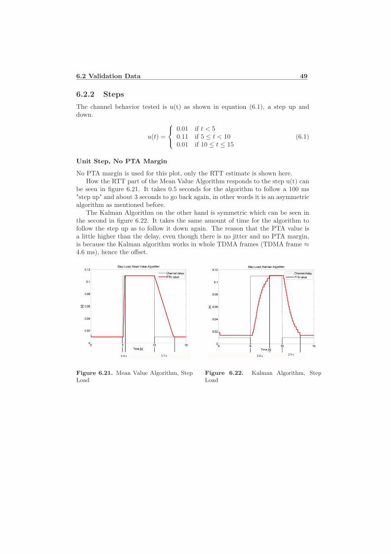
6.2.2 Steps
The channel behavior tested is u(t) as shown in equation (6.1), a step up anddown.
u(t) =
0.01 if t < 50.11 if 5 ≤ t < 100.01 if 10 ≤ t ≤ 15
(6.1)
Unit Step, No PTA Margin
No PTA margin is used for this plot, only the RTT estimate is shown here.How the RTT part of the Mean Value Algorithm responds to the step u(t) can
be seen in figure 6.21. It takes 0.5 seconds for the algorithm to follow a 100 ms"step up" and about 3 seconds to go back again, in other words it is an asymmetricalgorithm as mentioned before.
The Kalman Algorithm on the other hand is symmetric which can be seen inthe second in figure 6.22. It takes the same amount of time for the algorithm tofollow the step up as to follow it down again. The reason that the PTA value isa little higher than the delay, even though there is no jitter and no PTA margin,is because the Kalman algorithm works in whole TDMA frames (TDMA frame ≈4.6 ms), hence the offset.
Figure 6.21. Mean Value Algorithm, Step
Load
Figure 6.22. Kalman Algorithm, Step
Load
50 Algorithm Behavior
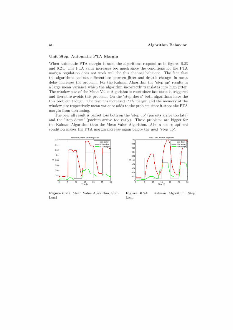
Unit Step, Automatic PTA Margin
When automatic PTA margin is used the algorithms respond as in figures 6.23and 6.24. The PTA value increases too much since the conditions for the PTAmargin regulation does not work well for this channel behavior. The fact thatthe algorithms can not differentiate between jitter and drastic changes in meandelay increases the problem. For the Kalman Algorithm the "step up" results ina large mean variance which the algorithm incorrectly translates into high jitter.The window size of the Mean Value Algorithm is reset since fast state is triggeredand therefore avoids this problem. On the "step down" both algorithms have thethis problem though. The result is increased PTA margin and the memory of thewindow size respectively mean variance adds to the problem since it stops the PTAmargin from decreasing.
The over all result is packet loss both on the "step up" (packets arrive too late)and the "step down" (packets arrive too early). These problems are bigger forthe Kalman Algorithm than the Mean Value Algorithm. Also a not so optimalcondition makes the PTA margin increase again before the next "step up".
0 5 10 15 20 25 300
0.02
0.04
0.06
0.08
0.1
0.12
0.14
0.16
Time [s]
[s]
Step Load, Mean Value Algorithm
abis delayPTA valuePTAmargin
Figure 6.23. Mean Value Algorithm, Step
Load
0 5 10 15 20 25 300
0.02
0.04
0.06
0.08
0.1
0.12
0.14
0.16
0.18
0.2
Time [s]
[s]
Step Load, Kalman Algorithm
abis delayPTA valuePTAmargin
Figure 6.24. Kalman Algorithm, Step
Load
Chapter 7
Simulations and Results
• The traffic model used in these simulations is a fixed rate source that senda packet of 32 bits with a data rate of 1600 bps, i.e. one packet every 20:thmillisecond
• The bundling time is set to 3 ms which means that it only adds an extradelay of 3 ms for each packet (no additional jitter)
• The bundling size is set to 310 bits so this margin never affects the simulation
• There is no random packet loss on the channel so all packet loss is due toearly or late arrival in the buffer
• The data rate of the channel is set to infinity (no limit)
The channel behaviors tested are low, medium, high and pyramid load. Lengthof a half pyramid: 100 s, number of steps: 100. All simulations are run for 400 sover 10 different seeds which gives a total of 4000 s. The data presented here isafter the algorithms have adjusted, i.e. the first data is truncated.
In the following sections the detailed simulations and results are stated. For asummary, see section 7.4.
51
52 Simulations and Results
7.1 Simulations with Fixed PTA
Three different fixed PTA values have been chosen to show how fixed PTA behavesand to give a reference point for the following simulations.
7.1.1 Simulations
The following settings are used for the simulations:
• Algorithm: Fixed PTA
• PTA:
– 0.0185 s (= PTA 3, see table 2.1 on page 10)
– 0.06 s (= PTA 12, see table 2.1 on page 10)
– 0.1108 s (= PTA 19, see table 2.1 on page 10)
• Automatic PTA margin: none
• PTA margin: N/A
• Alpha: N/A
7.1 Simulations with Fixed PTA 53
7.1.2 Simulation Results
PTA = 0.0185
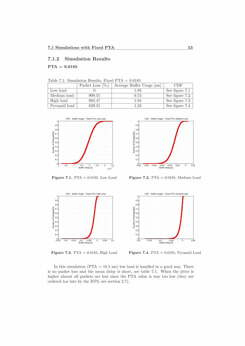
Table 7.1: Simulation Results, Fixed PTA = 0.0185Packet Loss [%�] Average Buffer Usage [ms] CDF
Low load 0 1.93 See figure 7.1Medium load 999.55 0.73 See figure 7.2High load 982.47 1.94 See figure 7.3Pyramid load 839.31 1.23 See figure 7.4
0 0.5 1 1.5 2 2.5 3 3.5
x 10−3
0
0.1
0.2
0.3
0.4
0.5
0.6
0.7
0.8
0.9
1
Buffer Delay [s]
Num
ber
of P
acka
ges[
%]
CDF − Buffer Usage − Fixed PTA, Low Load
Figure 7.1. PTA = 0.0185, Low Load
−0.06 −0.05 −0.04 −0.03 −0.02 −0.01 0 0.010
0.1
0.2
0.3
0.4
0.5
0.6
0.7
0.8
0.9
1
Buffer Delay [s]
Num
ber
of P
acka
ges[
%]
CDF − Buffer Usage − Fixed PTA, Medium Load
Figure 7.2. PTA = 0.0185, Medium Load
−0.25 −0.2 −0.15 −0.1 −0.05 0 0.05 0.10
0.1
0.2
0.3
0.4
0.5
0.6
0.7
0.8
0.9
1
Buffer Delay [s]
Num
ber
of P
acka
ges[
%]
CDF − Buffer Usage − Fixed PTA, High Load
Figure 7.3. PTA = 0.0185, High Load
−0.2 −0.15 −0.1 −0.05 0 0.050
0.1
0.2
0.3
0.4
0.5
0.6
0.7
0.8
0.9
1
Buffer Delay [s]
Num
ber
of P
acka
ges[
%]
CDF − Buffer Usage − Fixed PTA, Pyramid Load
Figure 7.4. PTA = 0.0185, Pyramid Load
In this simulation (PTA = 18.5 ms) low load is handled in a good way. Thereis no packet loss and the mean delay is short, see table 7.1. When the jitter ishigher almost all packets are lost since the PTA value is way too low (they areordered too late by the BTS, see section 2.7).
54 Simulations and Results
PTA = 0.06
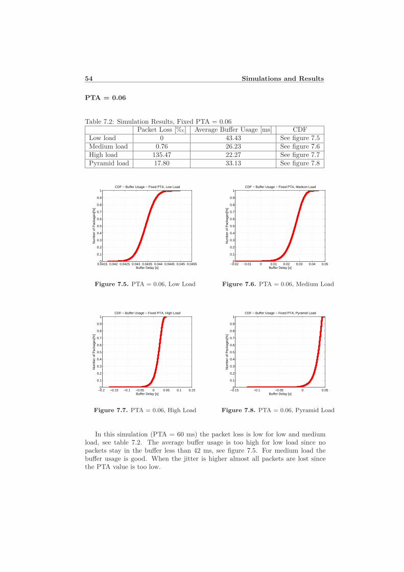
Table 7.2: Simulation Results, Fixed PTA = 0.06Packet Loss [%�] Average Buffer Usage [ms] CDF
Low load 0 43.43 See figure 7.5Medium load 0.76 26.23 See figure 7.6High load 135.47 22.27 See figure 7.7Pyramid load 17.80 33.13 See figure 7.8
0.0415 0.042 0.0425 0.043 0.0435 0.044 0.0445 0.045 0.04550
0.1
0.2
0.3
0.4
0.5
0.6
0.7
0.8
0.9
1
Buffer Delay [s]
Num
ber
of P
acka
ges[
%]
CDF − Buffer Usage − Fixed PTA, Low Load
Figure 7.5. PTA = 0.06, Low Load
−0.02 −0.01 0 0.01 0.02 0.03 0.04 0.050
0.1
0.2
0.3
0.4
0.5
0.6
0.7
0.8
0.9
1
Buffer Delay [s]
Num
ber
of P
acka
ges[
%]
CDF − Buffer Usage − Fixed PTA, Medium Load
Figure 7.6. PTA = 0.06, Medium Load
−0.2 −0.15 −0.1 −0.05 0 0.05 0.1 0.150
0.1
0.2
0.3
0.4
0.5
0.6
0.7
0.8
0.9
1
Buffer Delay [s]
Num
ber
of P
acka
ges[
%]
CDF − Buffer Usage − Fixed PTA, High Load
Figure 7.7. PTA = 0.06, High Load
−0.15 −0.1 −0.05 0 0.050
0.1
0.2
0.3
0.4
0.5
0.6
0.7
0.8
0.9
1
Buffer Delay [s]
Num
ber
of P
acka
ges[
%]
CDF − Buffer Usage − Fixed PTA, Pyramid Load
Figure 7.8. PTA = 0.06, Pyramid Load
In this simulation (PTA = 60 ms) the packet loss is low for low and mediumload, see table 7.2. The average buffer usage is too high for low load since nopackets stay in the buffer less than 42 ms, see figure 7.5. For medium load thebuffer usage is good. When the jitter is higher almost all packets are lost sincethe PTA value is too low.
7.1 Simulations with Fixed PTA 55
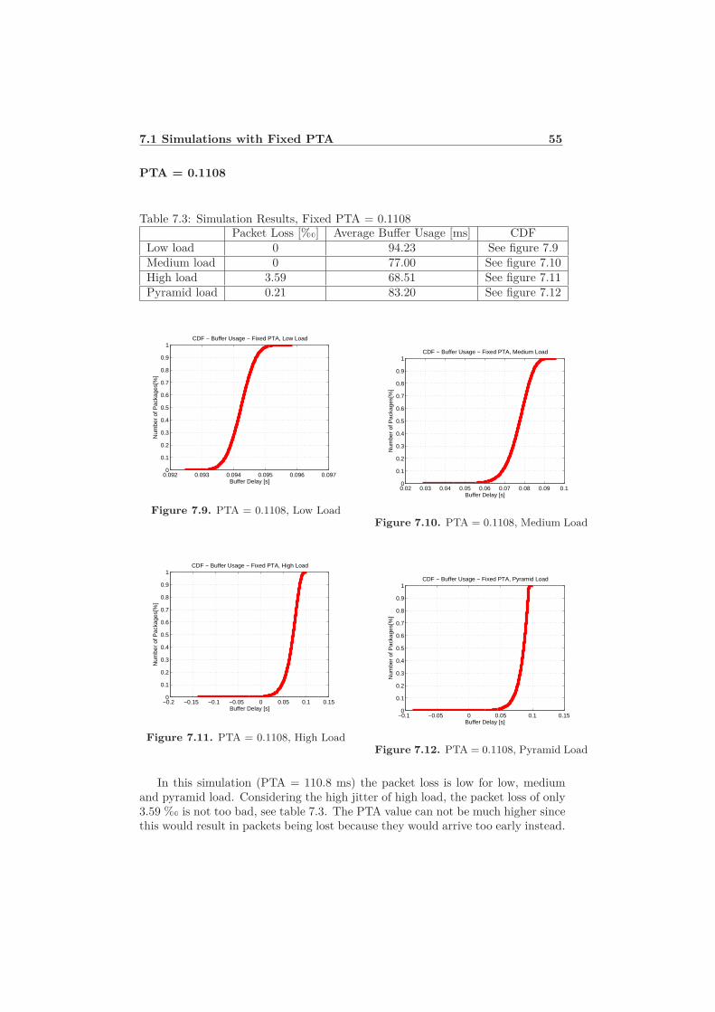
PTA = 0.1108
Table 7.3: Simulation Results, Fixed PTA = 0.1108Packet Loss [%�] Average Buffer Usage [ms] CDF
Low load 0 94.23 See figure 7.9Medium load 0 77.00 See figure 7.10High load 3.59 68.51 See figure 7.11Pyramid load 0.21 83.20 See figure 7.12
0.092 0.093 0.094 0.095 0.096 0.0970
0.1
0.2
0.3
0.4
0.5
0.6
0.7
0.8
0.9
1
Buffer Delay [s]
Num
ber
of P
acka
ges[
%]
CDF − Buffer Usage − Fixed PTA, Low Load
Figure 7.9. PTA = 0.1108, Low Load
0.02 0.03 0.04 0.05 0.06 0.07 0.08 0.09 0.10
0.1
0.2
0.3
0.4
0.5
0.6
0.7
0.8
0.9
1
Buffer Delay [s]
Num
ber
of P
acka
ges[
%]
CDF − Buffer Usage − Fixed PTA, Medium Load
Figure 7.10. PTA = 0.1108, Medium Load
−0.2 −0.15 −0.1 −0.05 0 0.05 0.1 0.150
0.1
0.2
0.3
0.4
0.5
0.6
0.7
0.8
0.9
1
Buffer Delay [s]
Num
ber
of P
acka
ges[
%]
CDF − Buffer Usage − Fixed PTA, High Load
Figure 7.11. PTA = 0.1108, High Load
−0.1 −0.05 0 0.05 0.1 0.150
0.1
0.2
0.3
0.4
0.5
0.6
0.7
0.8
0.9
1
Buffer Delay [s]
Num
ber
of P
acka
ges[
%]
CDF − Buffer Usage − Fixed PTA, Pyramid Load
Figure 7.12. PTA = 0.1108, Pyramid Load
In this simulation (PTA = 110.8 ms) the packet loss is low for low, mediumand pyramid load. Considering the high jitter of high load, the packet loss of only3.59 %� is not too bad, see table 7.3. The PTA value can not be much higher sincethis would result in packets being lost because they would arrive too early instead.
56 Simulations and Results
The high PTA value in this simulation results in packets being delayed in thebuffer an unnecessary long time for low and medium load, see figures 7.9 and 7.10.
7.2 Simulations with Fixed PTA Margin 57
7.2 Simulations with Fixed PTA Margin
One fixed PTA margin has been tested to show how it behaves and to give areference point for following simulations.
7.2.1 Simulations with Mean Value Algorithm
The following settings are used for the simulation:
• Algorithm: Mean Value Algorithm
• PTA: -
• Automatic PTA margin: none
• PTA margin: 0.06
• Alpha: 0.3
58 Simulations and Results
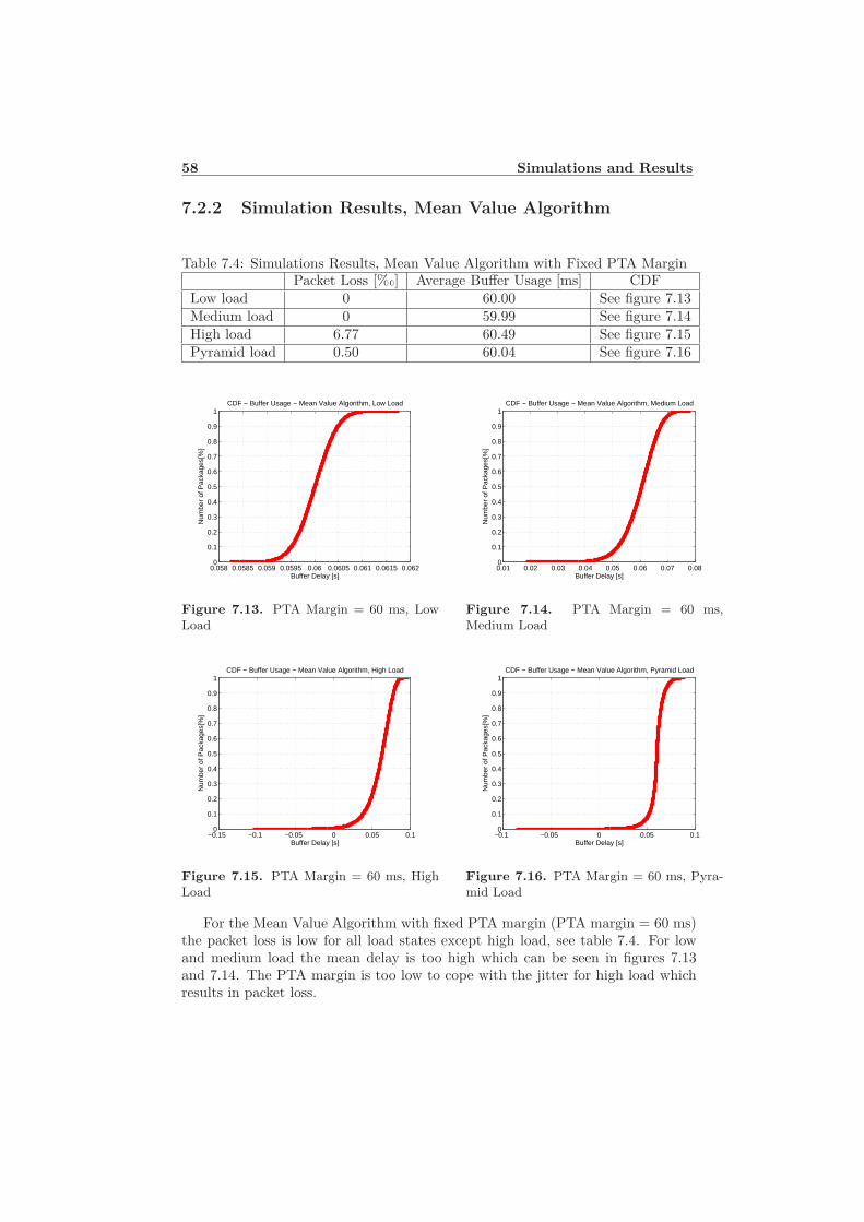
7.2.2 Simulation Results, Mean Value Algorithm
Table 7.4: Simulations Results, Mean Value Algorithm with Fixed PTA MarginPacket Loss [%�] Average Buffer Usage [ms] CDF
Low load 0 60.00 See figure 7.13Medium load 0 59.99 See figure 7.14High load 6.77 60.49 See figure 7.15Pyramid load 0.50 60.04 See figure 7.16
0.058 0.0585 0.059 0.0595 0.06 0.0605 0.061 0.0615 0.0620
0.1
0.2
0.3
0.4
0.5
0.6
0.7
0.8
0.9
1
Buffer Delay [s]
Num
ber
of P
acka
ges[
%]
CDF − Buffer Usage − Mean Value Algorithm, Low Load
Figure 7.13. PTA Margin = 60 ms, Low
Load
0.01 0.02 0.03 0.04 0.05 0.06 0.07 0.080
0.1
0.2
0.3
0.4
0.5
0.6
0.7
0.8
0.9
1
Buffer Delay [s]
Num
ber
of P
acka
ges[
%]
CDF − Buffer Usage − Mean Value Algorithm, Medium Load
Figure 7.14. PTA Margin = 60 ms,
Medium Load
−0.15 −0.1 −0.05 0 0.05 0.10
0.1
0.2
0.3
0.4
0.5
0.6
0.7
0.8
0.9
1
Buffer Delay [s]
Num
ber
of P
acka
ges[
%]
CDF − Buffer Usage − Mean Value Algorithm, High Load
Figure 7.15. PTA Margin = 60 ms, High
Load
−0.1 −0.05 0 0.05 0.10
0.1
0.2
0.3
0.4
0.5
0.6
0.7
0.8
0.9
1
Buffer Delay [s]
Num
ber
of P
acka
ges[
%]
CDF − Buffer Usage − Mean Value Algorithm, Pyramid Load
Figure 7.16. PTA Margin = 60 ms, Pyra-
mid Load
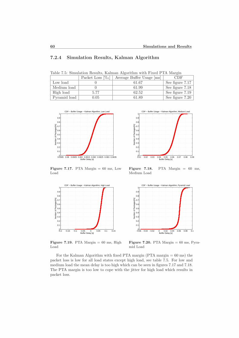
For the Mean Value Algorithm with fixed PTA margin (PTA margin = 60 ms)the packet loss is low for all load states except high load, see table 7.4. For lowand medium load the mean delay is too high which can be seen in figures 7.13and 7.14. The PTA margin is too low to cope with the jitter for high load whichresults in packet loss.

7.2 Simulations with Fixed PTA Margin 59
7.2.3 Simulations with Kalman Algorithm
The following settings are used for the simulation:
• Algorithm: Kalman Algorithm
• PTA: -
• Automatic PTA margin: none
• PTA margin: 0.06
• Alpha: N/A
60 Simulations and Results
7.2.4 Simulation Results, Kalman Algorithm
Table 7.5: Simulation Results, Kalman Algorithm with Fixed PTA MarginPacket Loss [%�] Average Buffer Usage [ms] CDF
Low load 0 61.67 See figure 7.17Medium load 0 61.99 See figure 7.18High load 5.77 62.52 See figure 7.19Pyramid load 0.05 61.89 See figure 7.20
0.0595 0.06 0.0605 0.061 0.0615 0.062 0.0625 0.063 0.06350
0.1
0.2
0.3
0.4
0.5
0.6
0.7
0.8
0.9
1
Buffer Delay [s]
Num
ber
of P
acka
ges[
%]
CDF − Buffer Usage − Kalman Algorithm, Low Load
Figure 7.17. PTA Margin = 60 ms, Low
Load
0.01 0.02 0.03 0.04 0.05 0.06 0.07 0.08 0.090
0.1
0.2
0.3
0.4
0.5
0.6
0.7
0.8
0.9
1
Buffer Delay [s]
Num
ber
of P
acka
ges[
%]
CDF − Buffer Usage − Kalman Algorithm, Medium Load
Figure 7.18. PTA Margin = 60 ms,
Medium Load
−0.2 −0.15 −0.1 −0.05 0 0.05 0.1 0.150
0.1
0.2
0.3
0.4
0.5
0.6
0.7
0.8
0.9
1
Buffer Delay [s]
Num
ber
of P
acka
ges[
%]
CDF − Buffer Usage − Kalman Algorithm, High Load
Figure 7.19. PTA Margin = 60 ms, High
Load
−0.06 −0.04 −0.02 0 0.02 0.04 0.06 0.08 0.10
0.1
0.2
0.3
0.4
0.5
0.6
0.7
0.8
0.9
1
Buffer Delay [s]
Num
ber
of P
acka
ges[
%]
CDF − Buffer Usage − Kalman Algorithm, Pyramid Load
Figure 7.20. PTA Margin = 60 ms, Pyra-
mid Load
For the Kalman Algorithm with fixed PTA margin (PTA margin = 60 ms) thepacket loss is low for all load states except high load, see table 7.5. For low andmedium load the mean delay is too high which can be seen in figures 7.17 and 7.18.The PTA margin is too low to cope with the jitter for high load which results inpacket loss.
7.3 Simulations with Automatic PTA Margin 61
7.3 Simulations with Automatic PTA Margin
7.3.1 Simulations with Mean Value Algorithm
The following settings are used for the simulation:
• Algorithm: Mean Value Algorithm
• PTA: -
• Automatic PTA margin: updated by window size
• PTA margin: 0.020 (initial)
• Alpha: 0.3
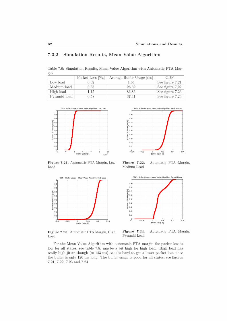
62 Simulations and Results
7.3.2 Simulation Results, Mean Value Algorithm
Table 7.6: Simulation Results, Mean Value Algorithm with Automatic PTA Mar-gin
Packet Loss [%�] Average Buffer Usage [ms] CDFLow load 0.02 1.64 See figure 7.21Medium load 0.83 26.59 See figure 7.22High load 1.15 86.86 See figure 7.23Pyramid load 0.58 37.41 See figure 7.24
−2 0 2 4 6 8 10
x 10−3
0
0.1
0.2
0.3
0.4
0.5
0.6
0.7
0.8
0.9
1
Buffer Delay [s]
Num
ber
of P
acka
ges[
%]
CDF − Buffer Usage − Mean Value Algorithm, Low Load
Figure 7.21. Automatic PTA Margin, Low
Load
−0.04 −0.02 0 0.02 0.04 0.060
0.1
0.2
0.3
0.4
0.5
0.6
0.7
0.8
0.9
1
Buffer Delay [s]
Num
ber
of P
acka
ges[
%]
CDF − Buffer Usage − Mean Value Algorithm, Medium Load
Figure 7.22. Automatic PTA Margin,
Medium Load
−0.1 −0.05 0 0.05 0.1 0.150
0.1
0.2
0.3
0.4
0.5
0.6
0.7
0.8
0.9
1
Buffer Delay [s]
Num
ber
of P
acka
ges[
%]
CDF − Buffer Usage − Mean Value Algorithm, High Load
Figure 7.23. Automatic PTA Margin, High
Load
−0.1 −0.05 0 0.05 0.1 0.150
0.1
0.2
0.3
0.4
0.5
0.6
0.7
0.8
0.9
1
Buffer Delay [s]
Num
ber
of P
acka
ges[
%]
CDF − Buffer Usage − Mean Value Algorithm, Pyramid Load
Figure 7.24. Automatic PTA Margin,
Pyramid Load
For the Mean Value Algorithm with automatic PTA margin the packet loss islow for all states, see table 7.8, maybe a bit high for high load. High load hasreally high jitter though (≈ 143 ms) so it is hard to get a lower packet loss sincethe buffer is only 120 ms long. The buffer usage is good for all states, see figures7.21, 7.22, 7.23 and 7.24.
7.3 Simulations with Automatic PTA Margin 63
7.3.3 Simulations with Kalman Algorithm
The following settings are used for the simulation:
• Algorithm: Kalman Algorithm
• PTA: -
• Automatic PTA margin: updated by mean variance
• PTA margin: 0.020 (initial)
• Alpha: N/A
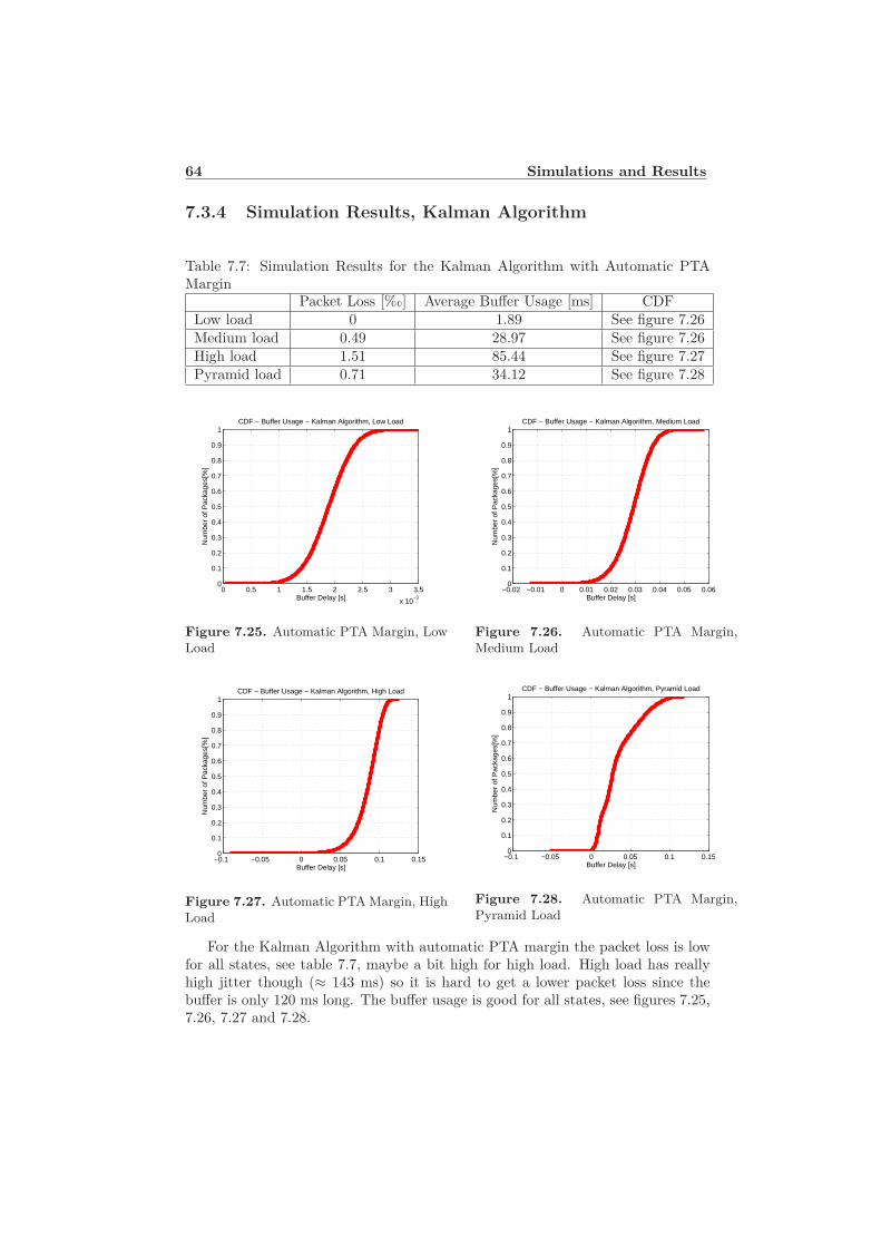
64 Simulations and Results
7.3.4 Simulation Results, Kalman Algorithm
Table 7.7: Simulation Results for the Kalman Algorithm with Automatic PTAMargin
Packet Loss [%�] Average Buffer Usage [ms] CDFLow load 0 1.89 See figure 7.26Medium load 0.49 28.97 See figure 7.26High load 1.51 85.44 See figure 7.27Pyramid load 0.71 34.12 See figure 7.28
0 0.5 1 1.5 2 2.5 3 3.5
x 10−3
0
0.1
0.2
0.3
0.4
0.5
0.6
0.7
0.8
0.9
1
Buffer Delay [s]
Num
ber
of P
acka
ges[
%]
CDF − Buffer Usage − Kalman Algorithm, Low Load
Figure 7.25. Automatic PTA Margin, Low
Load
−0.02 −0.01 0 0.01 0.02 0.03 0.04 0.05 0.060
0.1
0.2
0.3
0.4
0.5
0.6
0.7
0.8
0.9
1
Buffer Delay [s]
Num
ber
of P
acka
ges[
%]
CDF − Buffer Usage − Kalman Algorithm, Medium Load
Figure 7.26. Automatic PTA Margin,
Medium Load
−0.1 −0.05 0 0.05 0.1 0.150
0.1
0.2
0.3
0.4
0.5
0.6
0.7
0.8
0.9
1
Buffer Delay [s]
Num
ber
of P
acka
ges[
%]
CDF − Buffer Usage − Kalman Algorithm, High Load
Figure 7.27. Automatic PTA Margin, High
Load
−0.1 −0.05 0 0.05 0.1 0.150
0.1
0.2
0.3
0.4
0.5
0.6
0.7
0.8
0.9
1
Buffer Delay [s]
Num
ber
of P
acka
ges[
%]
CDF − Buffer Usage − Kalman Algorithm, Pyramid Load
Figure 7.28. Automatic PTA Margin,
Pyramid Load
For the Kalman Algorithm with automatic PTA margin the packet loss is lowfor all states, see table 7.7, maybe a bit high for high load. High load has reallyhigh jitter though (≈ 143 ms) so it is hard to get a lower packet loss since thebuffer is only 120 ms long. The buffer usage is good for all states, see figures 7.25,7.26, 7.27 and 7.28.
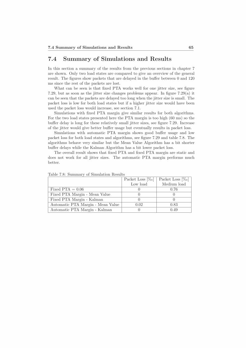
7.4 Summary of Simulations and Results 65
7.4 Summary of Simulations and Results
In this section a summary of the results from the previous sections in chapter 7are shown. Only two load states are compared to give an overview of the generalresult. The figures show packets that are delayed in the buffer between 0 and 120ms since the rest of the packets are lost.
What can be seen is that fixed PTA works well for one jitter size, see figure7.29, but as soon as the jitter size changes problems appear. In figure 7.29(a) itcan be seen that the packets are delayed too long when the jitter size is small. Thepacket loss is low for both load states but if a higher jitter size would have beenused the packet loss would increase, see section 7.1.
Simulations with fixed PTA margin give similar results for both algorithms.For the two load states presented here the PTA margin is too high (60 ms) so thebuffer delay is long for these relatively small jitter sizes, see figure 7.29. Increaseof the jitter would give better buffer usage but eventually results in packet loss.
Simulations with automatic PTA margin shows good buffer usage and lowpacket loss for both load states and algorithms, see figure 7.29 and table 7.8. Thealgorithms behave very similar but the Mean Value Algorithm has a bit shorterbuffer delays while the Kalman Algorithm has a bit lower packet loss.
The overall result shows that fixed PTA and fixed PTA margin are static anddoes not work for all jitter sizes. The automatic PTA margin performs muchbetter.
Table 7.8: Summary of Simulation ResultsPacket Loss [%�] Packet Loss [%�]
Low load Medium loadFixed PTA = 0.06 0 0.76Fixed PTA Margin - Mean Value 0 0Fixed PTA Margin - Kalman 0 0Automatic PTA Margin - Mean Value 0.02 0.83Automatic PTA Margin - Kalman 0 0.49
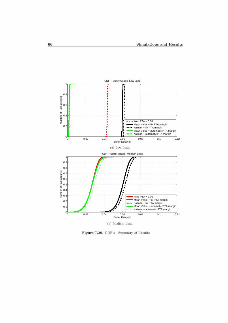
66 Simulations and Results
0 0.02 0.04 0.06 0.08 0.1 0.120
0.2
0.4
0.6
0.8
1
Buffer Delay [s]
Num
ber
of P
acka
ges[
%]
CDF − Buffer Usage, Low Load
fixed PTA = 0.06Mean Value − fix PTA marginKalman − fix PTA marginMean Value − automatic PTA marginKalman − automatic PTA margin
(a) Low Load
0 0.02 0.04 0.06 0.08 0.1 0.120
0.1
0.2
0.3
0.4
0.5
0.6
0.7
0.8
0.9
1
Buffer Delay [s]
Num
ber
of P
acka
ges[
%]
CDF − Buffer Usage, Medium Load
fixed PTA = 0.06Mean Value − fix PTA marginKalman − fix PTA marginMean Value − automatic PTA marginKalman − automatic PTA margin
(b) Medium Load
Figure 7.29. CDF’s - Summary of Results
Chapter 8
Algorithm Validation
The purpose of this simulation is to see how well the algorithms perform whenautomatic PTA margin is used. This is done by using new channel behaviors(the validation load states, see section 5.1.2). The following load states are used:low load 2, low-medium load, medium load 2, medium-high load, high load 2 andrandom load. The general conditions used for the validation simulations are thesame as the conditions for the simulations in chapter 7.
8.1 Simulation Settings
8.1.1 Simulation with Mean Value Algorithm
The following settings are used for the simulation:
• Algorithm: Mean Value Algorithm
• PTA: -
• Automatic PTA margin: updated by window size
• PTA margin: 0.020 (initial)
• Alpha: 0.3
8.1.2 Simulation with Kalman Algorithm
The following settings are used for the simulation:
• Algorithm: Kalman Algorithm
• PTA: -
• Automatic PTA margin: updated by mean variance
• PTA margin: 0.020 (initial)
• Alpha: N/A
67
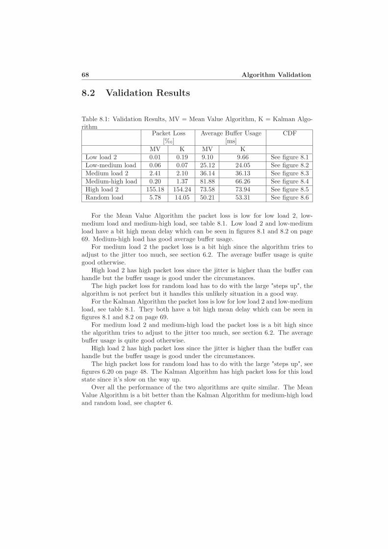
68 Algorithm Validation
8.2 Validation Results
Table 8.1: Validation Results, MV = Mean Value Algorithm, K = Kalman Algo-rithm
Packet Loss Average Buffer Usage CDF[%�] [ms]
MV K MV KLow load 2 0.01 0.19 9.10 9.66 See figure 8.1Low-medium load 0.06 0.07 25.12 24.05 See figure 8.2Medium load 2 2.41 2.10 36.14 36.13 See figure 8.3Medium-high load 0.20 1.37 81.88 66.26 See figure 8.4High load 2 155.18 154.24 73.58 73.94 See figure 8.5Random load 5.78 14.05 50.21 53.31 See figure 8.6
For the Mean Value Algorithm the packet loss is low for low load 2, low-medium load and medium-high load, see table 8.1. Low load 2 and low-mediumload have a bit high mean delay which can be seen in figures 8.1 and 8.2 on page69. Medium-high load has good average buffer usage.
For medium load 2 the packet loss is a bit high since the algorithm tries toadjust to the jitter too much, see section 6.2. The average buffer usage is quitegood otherwise.
High load 2 has high packet loss since the jitter is higher than the buffer canhandle but the buffer usage is good under the circumstances.
The high packet loss for random load has to do with the large "steps up", thealgorithm is not perfect but it handles this unlikely situation in a good way.
For the Kalman Algorithm the packet loss is low for low load 2 and low-mediumload, see table 8.1. They both have a bit high mean delay which can be seen infigures 8.1 and 8.2 on page 69.
For medium load 2 and medium-high load the packet loss is a bit high sincethe algorithm tries to adjust to the jitter too much, see section 6.2. The averagebuffer usage is quite good otherwise.
High load 2 has high packet loss since the jitter is higher than the buffer canhandle but the buffer usage is good under the circumstances.
The high packet loss for random load has to do with the large "steps up", seefigures 6.20 on page 48. The Kalman Algorithm has high packet loss for this loadstate since it’s slow on the way up.
Over all the performance of the two algorithms are quite similar. The MeanValue Algorithm is a bit better than the Kalman Algorithm for medium-high loadand random load, see chapter 6.
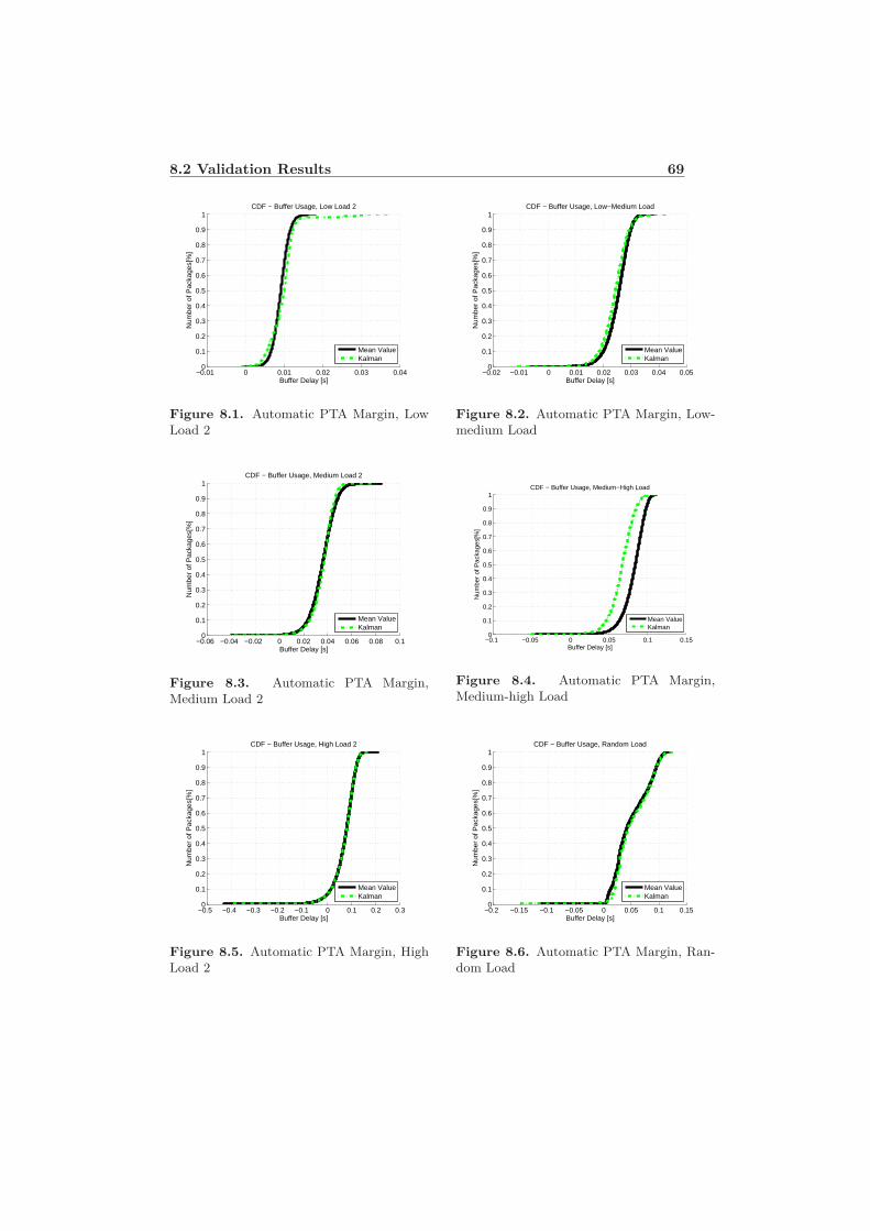
8.2 Validation Results 69
−0.01 0 0.01 0.02 0.03 0.040
0.1
0.2
0.3
0.4
0.5
0.6
0.7
0.8
0.9
1
Buffer Delay [s]
Num
ber
of P
acka
ges[
%]
CDF − Buffer Usage, Low Load 2
Mean ValueKalman
Figure 8.1. Automatic PTA Margin, Low
Load 2
−0.02 −0.01 0 0.01 0.02 0.03 0.04 0.050
0.1
0.2
0.3
0.4
0.5
0.6
0.7
0.8
0.9
1
Buffer Delay [s]
Num
ber
of P
acka
ges[
%]
CDF − Buffer Usage, Low−Medium Load
Mean ValueKalman
Figure 8.2. Automatic PTA Margin, Low-
medium Load
−0.06 −0.04 −0.02 0 0.02 0.04 0.06 0.08 0.10
0.1
0.2
0.3
0.4
0.5
0.6
0.7
0.8
0.9
1
Buffer Delay [s]
Num
ber
of P
acka
ges[
%]
CDF − Buffer Usage, Medium Load 2
Mean ValueKalman
Figure 8.3. Automatic PTA Margin,
Medium Load 2
−0.1 −0.05 0 0.05 0.1 0.150
0.1
0.2
0.3
0.4
0.5
0.6
0.7
0.8
0.9
1
Buffer Delay [s]
Num
ber
of P
acka
ges[
%]
CDF − Buffer Usage, Medium−High Load
Mean ValueKalman
Figure 8.4. Automatic PTA Margin,
Medium-high Load
−0.5 −0.4 −0.3 −0.2 −0.1 0 0.1 0.2 0.30
0.1
0.2
0.3
0.4
0.5
0.6
0.7
0.8
0.9
1
Buffer Delay [s]
Num
ber
of P
acka
ges[
%]
CDF − Buffer Usage, High Load 2
Mean ValueKalman
Figure 8.5. Automatic PTA Margin, High
Load 2
−0.2 −0.15 −0.1 −0.05 0 0.05 0.1 0.150
0.1
0.2
0.3
0.4
0.5
0.6
0.7
0.8
0.9
1
Buffer Delay [s]
Num
ber
of P
acka
ges[
%]
CDF − Buffer Usage, Random Load
Mean ValueKalman
Figure 8.6. Automatic PTA Margin, Ran-
dom Load

Chapter 9
Conclusions and Discussion
By performing a statistical study through pinging, the characteristics of a generalIP network were observed. The results from this study made it possible to achievea good enough Abis model to be able to develop algorithms for dynamic jitterbuffering.
9.1 Analysis of Results
The results from the simulations with Fixed PTA shows that this method is staticand it is impossible to choose a PTA value that works satisfactory for differentchannel behaviors. If the PTA value fits one channel behavior it results in packetloss or high mean delay for others.
When the algorithms are used together with fixed PTA margin the resultis better since the estimates of the round trip times follows the channel behavior.It is still static though in some sense since it is a fixed margin added to the RTTestimates. Hence this method has the same problem as Fixed PTA by only workingwell for one channel behavior.
This shows the need for a dynamic jitter buffer, i.e. that the PTA value doesnot have any static part.
The results from the simulations with automatic PTA margin shows thatthe relation between packet loss and average buffer usage is satisfactory for allsimulation load states. Packets are not delayed more than needed and still withouttoo much packet loss. When using validation states, i.e. new jitter sizes that hasnot been used for development of the algorithms, the results are not quite as good.In most cases the PTA value is a bit too high so the mean buffer delay gets longerbut the packet loss is low. In one case it is the other way around so the packetloss is slightly high.
9.1.1 Comparison of Algorithms
The main difference between the algorithms is that the asymmetric Mean ValueAlgorithm is faster on the way up than the symmetric Kalman Algorithm. This
71
72 Conclusions and Discussion
is the reason why the packet loss is higher for the Kalman Algorithm when usingrandom load which has sudden changes in jitter level. It takes about the sametime for the two algorithms to adjust on the way down from high to low jitter.
When it comes to adjustment of the PTA value, when initializing the algo-rithms, the results show that the Kalman Algorithm sometimes over compensateswhen the Mean Value Algorithm does not. But when the later does over compen-sate, it takes about twice as long time to adjust. The adjustment time is not reallya problem when the channel delay changes slowly (on the way down). But if thechannel delay changes very fast, like the unit step tested, packets might be lostbecause the PTA value decreases too slowly. That kind of behavior is probablyunlikely in a real network though.
Another difference is that since the Kalman Algorithm works in whole TDMAframes it can not be as fine-tuned as the Mean Value Algorithm. This can resultin an approximately 4 ms larger PTA value which only matters when the jitter isvery low.
9.2 Future Studies
To get a more complete picture of how the algorithms would perform in a realnetwork, more extensive simulations with all relevant protocol layers should bemade. For example using several users or at least a source with varying data rateso the bundling can be tested with the algorithms. Since we have not looked atthe air interface and the radio conditions this would be of interest to observe theend to end performance.
Something that could be done to develop the PTA estimation a bit further isto consider that the time slots in a TDMA frame are sent with different delaysfrom the BTS. In reality the TDMA structure is built in a way so that the timeslots are transmitted after each other which results in that time slot 0 are sentabout 1 ms before time slot 7. This would make the simulations resemble realityeven better.
In our implementation of the bundling in the Abis protocol an error message isreceived if a packet is 1500 bytes or larger since that is the approximate maximumsize of an IP packet (over Ethernet). Instead the packet should be split into smallerpackets.
Something that ought to be done is to make the Kalman Algorithm faster (bychanging the design parameters) and then evaluate if the behavior improves. Thepacket loss will most likely be lower for random and step load but it might affectother load states in a negative way.
What is probably needed to improve the PTA margin handling is to divide thebuffer into more slots which would give less quantization error. The conditionsfor the PTA margin also needs to be tuned a bit better so that no conditionsconflict. With higher buffer quantization it might also be possible to avoid usingthe mean variance the way we have. This would reduce problems with high and/oroscillating PTA margin. It would also take away the issue that the algorithmincorrectly interprets a fast change of delay as jitter.
9.2 Future Studies 73
In our statistical study we noticed some spikes in the RTT plots of the realdelays. These are still unexplained and needs to be investigated further. We thinkit is a phenomenon created by the computers involved in the pinging. Over all,a larger statistical study would be beneficial, mainly to see how a real networkbehaves over a long period of time. Are there any drastic jumps in jitter size?What is the maximum jitter? Maybe other IP networks besides internet shouldbe tested?

Bibliography
[1] Ericsson AB. Gprs system survey. LZT 123 5347 R4A, 2005.
[2] Ericsson AB. User description, flexible abis. 235/1553-HSC 103 12/11 Uen A,2007.
[3] Ericsson AB. User description, abis optimization. 264/1553-HSC 103 12/13Uen A, 2008.
[4] Ericsson AB. User description, abis over ip. 263/1553-HSC 103 12/13 Uen B,2008.
[5] Ericsson Radio Systems AB. Gsm system survey. EN/LZT 123 3321 R4A,1998.
[6] Fredrik Gustafsson, Lennart Ljung, and Mille Millnert. Signalbehandling.ISBN 978-91-44-01709-9.
[7] VoIPForo. Quality of service: Jitter. URL:http://www.en.voipforo.com/QoS/QoSJitter.php [2008-09-11], 2008.
75

Appendix A
Ping - Histograms of RoundTrip Times
77
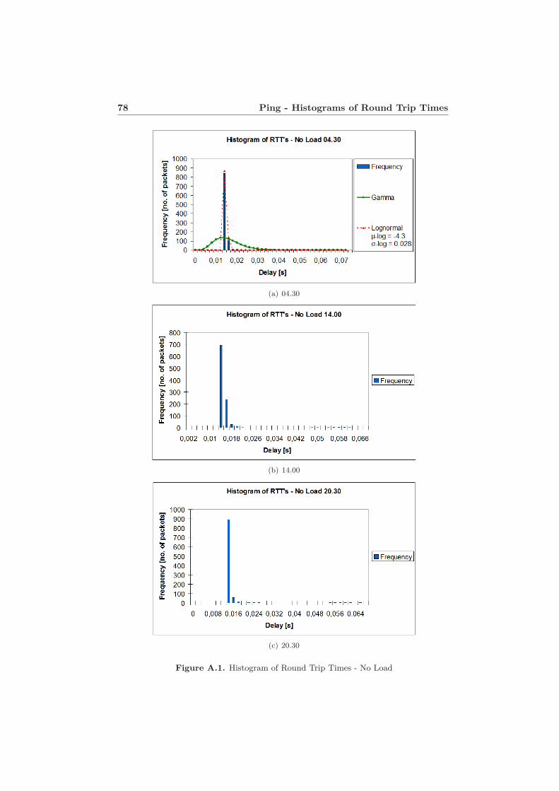
78 Ping - Histograms of Round Trip Times
(a) 04.30
(b) 14.00
(c) 20.30
Figure A.1. Histogram of Round Trip Times - No Load
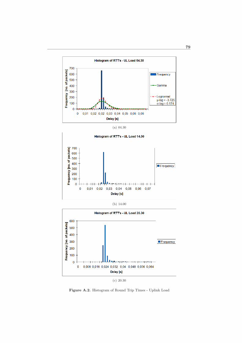
79
(a) 04.30
(b) 14.00
(c) 20.30
Figure A.2. Histogram of Round Trip Times - Uplink Load
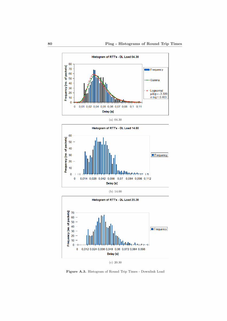
80 Ping - Histograms of Round Trip Times
(a) 04.30
(b) 14.00
(c) 20.30
Figure A.3. Histogram of Round Trip Times - Downlink Load
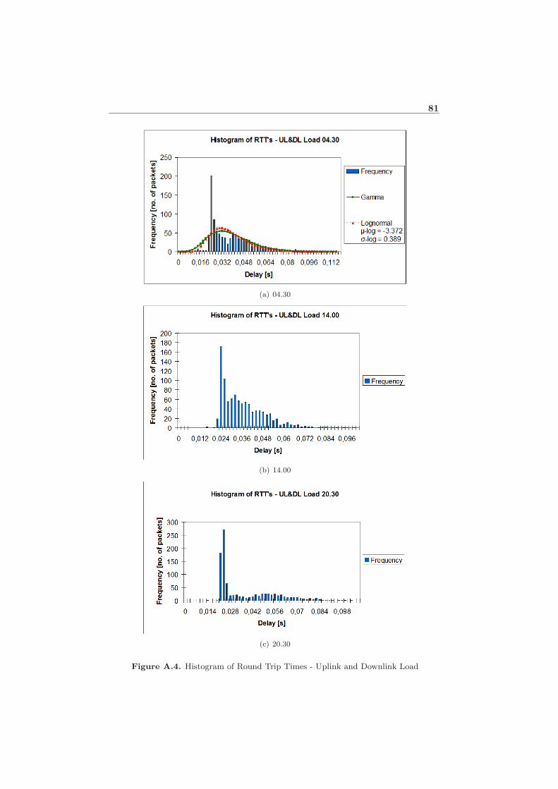
81
(a) 04.30
(b) 14.00
(c) 20.30
Figure A.4. Histogram of Round Trip Times - Uplink and Downlink Load
Appendix B
Ping - Round Trip Times
82
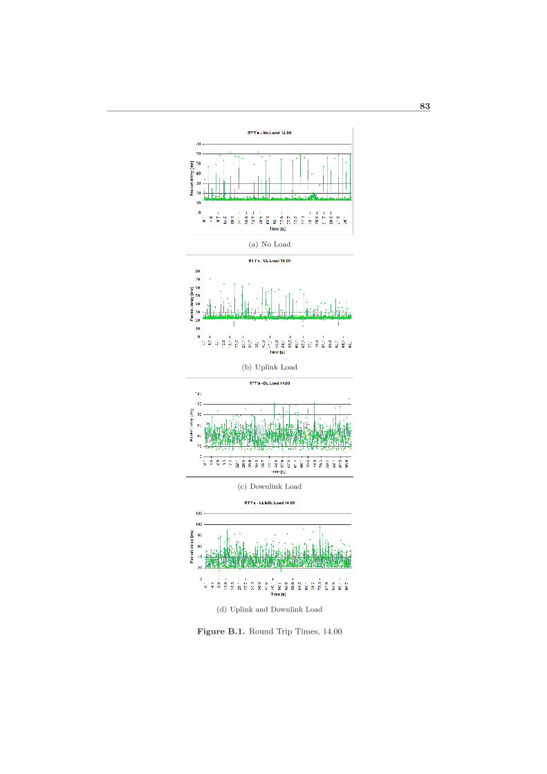
83
(a) No Load
(b) Uplink Load
(c) Downlink Load
(d) Uplink and Downlink Load
Figure B.1. Round Trip Times, 14.00

Upphovsrätt
Detta dokument hålls tillgängligt på Internet — eller dess framtida ersättare —under 25 år från publiceringsdatum under förutsättning att inga extraordinäraomständigheter uppstår.
Tillgång till dokumentet innebär tillstånd för var och en att läsa, ladda ner,skriva ut enstaka kopior för enskilt bruk och att använda det oförändrat för icke-kommersiell forskning och för undervisning. Överföring av upphovsrätten vid ensenare tidpunkt kan inte upphäva detta tillstånd. All annan användning av doku-mentet kräver upphovsmannens medgivande. För att garantera äktheten, säker-heten och tillgängligheten finns det lösningar av teknisk och administrativ art.
Upphovsmannens ideella rätt innefattar rätt att bli nämnd som upphovsmani den omfattning som god sed kräver vid användning av dokumentet på ovan be-skrivna sätt samt skydd mot att dokumentet ändras eller presenteras i sådan formeller i sådant sammanhang som är kränkande för upphovsmannens litterära ellerkonstnärliga anseende eller egenart.
För ytterligare information om Linköping University Electronic Press se för-lagets hemsida http://www.ep.liu.se/
Copyright
The publishers will keep this document online on the Internet — or its possi-ble replacement — for a period of 25 years from the date of publication barringexceptional circumstances.
The online availability of the document implies a permanent permission foranyone to read, to download, to print out single copies for his/her own use andto use it unchanged for any non-commercial research and educational purpose.Subsequent transfers of copyright cannot revoke this permission. All other uses ofthe document are conditional on the consent of the copyright owner. The publisherhas taken technical and administrative measures to assure authenticity, securityand accessibility.
According to intellectual property law the author has the right to be mentionedwhen his/her work is accessed as described above and to be protected againstinfringement.
For additional information about the Linköping University Electronic Pressand its procedures for publication and for assurance of document integrity, pleaserefer to its www home page: http://www.ep.liu.se/
c© Gabriella Ferm och Jonas Jarledal