Instream Biological Assessment MonitoringProtocols: Benthic Macroinvertebrates

June 1994Publication #94-113

printed on recycled paper

The Department of Ecology is an Equal Opportunity andAffirmative Action employer and shall not discriminate on thebasis of race, creed, color, national origin, sex, marital status,

sexual orientation, age, religion, or disability as defined byapplicable state and/or federal regulations and statutes.

If you have special accommodation needs, please contact theEnvironmental Investigations and Laboratory Services Program,

Ambient Monitoring Section, Rob Plotnikoff at (206) 407-6687 (voice).Ecology's telecommunications device for the deaf (TDD) number

at Ecology Headquarters is (206) 407-6006.

For additional copies of this publication, please contact:

Department of EcologyPublications Distributions Office

at Post Office Box 47600(206) 407-7472

Refer to Publication Number 94-113

Instream Biological Assessment MonitoringProtocols: Benthic Macroinvertebrates

byR.W. Plotnikoff

Environmental Investigationsand Laboratory Services

Ambient Monitoring SectionWashington State Department of Ecology

Post Office Box 47710Olympia, Washington 98504-7710

June 1994Publication #94-113

TABLE OF CONTENTS

Page

INTRODUCTION . . . . . . . . . . . . . . . . . . . . . . . . . . . . . . . . . . . . . . . . . . . . . . . . . . . 1Purpose of this Document . . . . . . . . . . . . . . . . . . . . . . . . . . . . . . . . . . . . . . . . 1Background . . . . . . . . . . . . . . . . . . . . . . . . . . . . . . . . . . . . . . . . . . . . . . . . . . 1Purpose for Monitoring Stream Biology . . . . . . . . . . . . . . . . . . . . . . . . . . . . . . . 1Ambient Biological Assessment Monitoring . . . . . . . . . . . . . . . . . . . . . . . . . . . . 2

Long-Term Ambient Monitoring. . . . . . . . . . . . . . . . . . . . . . . . . . . . . . . 2Applications for Stream Biology Information. . . . . . . . . . . . . . . . . . . . . . 3

PROJECT ORGANIZATION . . . . . . . . . . . . . . . . . . . . . . . . . . . . . . . . . . . . . . . . . . . 3Personnel. . . . . . . . . . . . . . . . . . . . . . . . . . . . . . . . . . . . . . . . . . . . . . . . . . . . 3Experience . . . . . . . . . . . . . . . . . . . . . . . . . . . . . . . . . . . . . . . . . . . . . . . . . . . 3

STUDY DESIGN . . . . . . . . . . . . . . . . . . . . . . . . . . . . . . . . . . . . . . . . . . . . . . . . . . . 4Sampling Strategy . . . . . . . . . . . . . . . . . . . . . . . . . . . . . . . . . . . . . . . . . . . . . . 4

General Design . . . . . . . . . . . . . . . . . . . . . . . . . . . . . . . . . . . . . . . . . . . 4Sample Site Selection Criteria . . . . . . . . . . . . . . . . . . . . . . . . . . . . . . . . 5Regional Basins/Watersheds . . . . . . . . . . . . . . . . . . . . . . . . . . . . . . . . . . 5Ecoregion Representation . . . . . . . . . . . . . . . . . . . . . . . . . . . . . . . . . . . . 5Representative Land Uses . . . . . . . . . . . . . . . . . . . . . . . . . . . . . . . . . . . 6Index Period . . . . . . . . . . . . . . . . . . . . . . . . . . . . . . . . . . . . . . . . . . . . . 7

DATA QUALITY OBJECTIVES . . . . . . . . . . . . . . . . . . . . . . . . . . . . . . . . . . . . . . . . 8Precision . . . . . . . . . . . . . . . . . . . . . . . . . . . . . . . . . . . . . . . . . . . . . . . . . . . . 8Bias . . . . . . . . . . . . . . . . . . . . . . . . . . . . . . . . . . . . . . . . . . . . . . . . . . . . . . . . 8Representativeness . . . . . . . . . . . . . . . . . . . . . . . . . . . . . . . . . . . . . . . . . . . . . . 8Completeness . . . . . . . . . . . . . . . . . . . . . . . . . . . . . . . . . . . . . . . . . . . . . . . . . 8Comparability . . . . . . . . . . . . . . . . . . . . . . . . . . . . . . . . . . . . . . . . . . . . . . . . . 9

SAFETY PROCEDURES . . . . . . . . . . . . . . . . . . . . . . . . . . . . . . . . . . . . . . . . . . . . . . 9Field and Laboratory Preservatives . . . . . . . . . . . . . . . . . . . . . . . . . . . . . . . . . . 9Miscellaneous . . . . . . . . . . . . . . . . . . . . . . . . . . . . . . . . . . . . . . . . . . . . . . . . 10

FIELD OPERATIONS . . . . . . . . . . . . . . . . . . . . . . . . . . . . . . . . . . . . . . . . . . . . . . . 10Macroinvertebrate Sampling . . . . . . . . . . . . . . . . . . . . . . . . . . . . . . . . . . . . . . 10

Sampling Techniques . . . . . . . . . . . . . . . . . . . . . . . . . . . . . . . . . . . . . 10Habitat Survey . . . . . . . . . . . . . . . . . . . . . . . . . . . . . . . . . . . . . . . . . . . . . . . 11

Habitat Variables . . . . . . . . . . . . . . . . . . . . . . . . . . . . . . . . . . . . . . . . 11Watershed Land Use Survey . . . . . . . . . . . . . . . . . . . . . . . . . . . . . . . . 14

Surface Water Monitoring. . . . . . . . . . . . . . . . . . . . . . . . . . . . . . . . . . . . . . . 14Water Quality Analyses. . . . . . . . . . . . . . . . . . . . . . . . . . . . . . . . . . . . 14Quality Assurance. . . . . . . . . . . . . . . . . . . . . . . . . . . . . . . . . . . . . . . . 15

i

TABLE OF CONTENTS

LABORATORY SAMPLE PROCESSING . . . . . . . . . . . . . . . . . . . . . . . . . . . . . . . . . 15Benthic Macroinvertebrate and CPOM Samples . . . . . . . . . . . . . . . . . . . . . . . . 15Benthic Macroinvertebrate Identification . . . . . . . . . . . . . . . . . . . . . . . . . . . . . 15Laboratory Quality Assurance. . . . . . . . . . . . . . . . . . . . . . . . . . . . . . . . . . . . . 16

Macroinvertebrate Sorting . . . . . . . . . . . . . . . . . . . . . . . . . . . . . . . . . . 16Macroinvertebrate Identification . . . . . . . . . . . . . . . . . . . . . . . . . . . . . . 17

DATA ANALYSIS . . . . . . . . . . . . . . . . . . . . . . . . . . . . . . . . . . . . . . . . . . . . . . . . . 17General Analytical Procedures . . . . . . . . . . . . . . . . . . . . . . . . . . . . . . . . . . . . 17

Biological Metrics . . . . . . . . . . . . . . . . . . . . . . . . . . . . . . . . . . . . . . . . 17Ordination: Identifying Unique Ecosystem Functions . . . . . . . . . . . . . . . 19Land-Use (Geographical Information Systems) . . . . . . . . . . . . . . . . . . . . 19Similarity to an Indicator Assemblage. . . . . . . . . . . . . . . . . . . . . . . . . . 20Trend or Temporal Analysis . . . . . . . . . . . . . . . . . . . . . . . . . . . . . . . . . 20

DATA MANAGEMENT . . . . . . . . . . . . . . . . . . . . . . . . . . . . . . . . . . . . . . . . . . . . . 21Current Data Management Procedures . . . . . . . . . . . . . . . . . . . . . . . . . . . . . . . 21Compatible Databases . . . . . . . . . . . . . . . . . . . . . . . . . . . . . . . . . . . . . . . . . . 21

REGIONAL ENVIRONMENTAL MONITORING AND ASSESSMENT PROGRAM(R-EMAP) . . . . . . . . . . . . . . . . . . . . . . . . . . . . . . . . . . . . . . . . . . . . . . . . . . 22Coordination with R-EMAP . . . . . . . . . . . . . . . . . . . . . . . . . . . . . . . . . . . . . . 22

LITERATURE CITED . . . . . . . . . . . . . . . . . . . . . . . . . . . . . . . . . . . . . . . . . . . . . . . 24

APPENDIX A. Washington State Department of Ecology: Watershed Approach to WaterQuality Management

APPENDIX B. Site Locations of Biological Assessments in Washington State

APPENDIX C. Field Forms for Chemical and Physical Habitat Assessments

APPENDIX D. Data Management: Biological Information and Habitat Variables

ii

ACKNOWLEDGEMENTS

I would like to extend my gratitude to Larry Lake (Ambient Monitoring Section) andDave Terpening (U.S. EPA - Region 10) who assisted with the majority of field sampling thisyear. Additional field assistance was provided by Gretchen Hayslip (EPA), Bruce Duncan(EPA), Joe Goulet (EPA), Rob Pedersen (EPA), Bill Ehinger (Ecology - Ambient MonitoringSection) and Ken Dzinbal (Ecology - Ambient Monitoring Section). Extensive review of thedraft copies were provided by Ken Dzinbal and his effort improved this documentdramatically. I am indebted to Leska Fore and Jim Karr (Institute for Environmental Studies -University of Washington) for their critical review of two draft versions in which theyprovided immeasurable assistance. I would also like to thank other reviewers from theEnvironmental Investigations and Laboratory Services Program (Washington State Departmentof Ecology) for their assistance in final preparation of this document.

iii

INTRODUCTION

Purpose of this Document

This document describes Washington State Department of Ecology's Freshwater AmbientBiological Assessment Program. Outlined within the document is: 1) the sampling design, 2)the site selection process, 3) field implementation, 4) laboratory processing of data, and 5)analysis and interpretation of data that will be used in conducting this program. Thedocument also includes all of the elements necessary to serve as a Quality Assurance ProjectPlan (QAPP) to guide the project.

Background

The Federal Clean Water Act (Section 101) mandates the development of water managementprograms that evaluate, restore, and maintain the chemical, physical, and biological integrityof the Nation's waters (U.S. EPA, 1990). Traditional measurements of chemical and physicalcomponents of rivers and streams do not provide sufficient information to detect or resolve allsurface water problems. Biological evaluation of surface waters provides a broader approachbecause degradation of sensitive ecosystem processes are more frequently identified. Biological assessments supplement chemical evaluation by:

a) directly measuring the most sensitive resources at risk,b) measuring a stream component that integrates and reflects human influence over

time, andc) providing a diagnostic tool that synthesizes chemical, physical, and biological

perturbations (Hayslip, 1993).

Biological assessment in Washington State has historically been used on a project-specificbasis. Stream impacts have been documented using an upstream/downstream approach atspecific facilities (i.e., industrial and wastewater treatment plants), or as a regional project toevaluate sampling and analytical protocols (e.g., Plotnikoff, 1992).

Ambient biological assessment of rivers and streams was initiated by the Washington StateDepartment of Ecology (Ecology) in summer 1993. Condition of stream biology throughoutthe state has not previously been defined. This project is being conducted to consistently andcomprehensively determine biological integrity in stream macroinvertebrate communities.

Purpose for Monitoring Stream Biology

Failure to demonstrate conservation and protection of water quality in the United States hasprompted alternative directions for evaluating the resource. The continued decline in diversityof aquatic species throughout North and South America attests to the urgency with whichconservation of our water resources must be addressed (Allan and Flecker, 1993). Maintenance of biological integrity was defined by Karr and Dudley (1981) as:

1

"a balanced, integrated, adaptive community of organisms having a speciescomposition, diversity, and functional organization comparable to that of naturalhabitat of the region."

Karr (1991) examined some of the reasons why evaluation of aquatic resources has taken solong in employing biological information. He also provided examples of how biologicalassessment of running water is applied in environmental evaluation and how powerful a toolthis method is. Inclusion of multiple levels of biological measures (e.g., community structureand function, bioassays, tissue analysis, biomarkers) enhances the ability for accuratelydiagnosing the source of degradation.

The Washington State Department of Ecology (Ecology) recognizes the need for monitoringadditional components of the ecosystem that are more sensitive to human influence anddegradation than traditional monitoring activities have detected. Societal awareness forenvironmental quality has placed increased pressure on efficient regulation of naturalresources. Stewardship of these resources requires us to apply the most effective evaluationtechniques available. Our biological database is comprised of continuous monitoringinformation that describes the condition of aquatic resources in greater detail. The biologicalinformation is also used to confirm or validate interpretations derived from chemical andphysical monitoring programs.

Ambient Biological Assessment Monitoring

The Ecology Ambient Biological Assessment Monitoring objectives are:

• to define and document baseline conditions of instream biology, and• to measure spatial and temporal variability of population and community attributes.

Biological monitoring focuses on wadeable stream reaches at middle to upper locations inwatersheds. Biological assessment effectively describes water quality and physical impactsfrom broad scale land use changes caused by forest practices, agriculture, and urbanization.

Long-Term Ambient Monitoring

The primary goal of the Freshwater Ambient Biological Assessment Program is to collectlong-term information to refine knowledge of stream conditions. Long-term (multiple year)data are critical for providing measures that will describe typical interannual variability anddefine reference conditions. Environmental conditions (e.g., climate, intensity of naturaldisturbance) vary between years and subsequently influence stream biological communities. A key step in differentiating natural environmental influences from anthropogenic influencesis to measure interannual variability.

Reference conditions are especially important in developing biologically meaningful criteria toprotect resources. The reference condition reflects biological community potential in a

2

stream, and is also used to describe spatial and temporal trends. But to be effective,biological criteria should reflect the variety of natural conditions that occur within a set ofsimilar stream types. This is best achieved through long-term monitoring of reference anddegraded sites.

Applications for Stream Biology Information

Ecology can currently use stream biological information to supplement the Statewide WaterQuality Assessment Report (Section 305(b) of the Federal Clean Water Act), to prioritizestreams/rivers for intensive surveys and development of total maximum daily loads (TMDL's,Section 303(d) of the Federal Clean Water Act), and to assess the success of pollutionabatement programs (Section 319 of the Federal Clean Water Act). Over a longer term,stream biological information will support development of narrative (and eventuallynumerical) biological water quality criteria.

Many federal agencies and local governments also need stream biological information. Newmandates for federal agencies such as the U.S. Forest Service, Bureau of Land Management,U.S. Geological Survey, and the U.S. Fish and Wildlife Service require them to evaluate thepresent condition of water resources within their jurisdictions. These biological evaluationsassist in management decisions to preserve existing sensitive fish and wildlife populations andto restore water resources to their potential. A pre-existing baseline of stream biologicalinformation is also very helpful for local governments in implementing water quality andstream habitat improvement programs.

PROJECT ORGANIZATION

Personnel

Field work is completed with at least two personnel who gather samples and measure physicalvariables at each site. The project leader designs and directs the components of the biologicalassessment program. A junior scientist or environmental technician collects biological andphysical data from rivers and streams, performs laboratory sample sorting and taxonomicidentifications, and records data in a database.

Experience

The Senior Scientist must be able to: 1) independently design a project and direct field work,2) identify most benthic macroinvertebrate taxa to species, with available taxonomic literature,3) understand and apply current stream ecology theory for interpretation of the biologicaldata, 4) operate a variety of computer software including word processors, spreadsheets,statistical programs, and databases, and 5) supervise more junior personnel. Qualifications forthe junior scientist/environmental technician are: 1) ability to understand project design andimplement the components, 2) efficiently use taxonomic keys and identify most taxa to genus,

3

3) have a general knowledge of computer software operation, and 4) to operate streamsampling equipment for measuring biological communities and physical variables.

STUDY DESIGN

Sampling Strategy

General Design

This program uses representative multiple-habitat sampling of benthic macroinvertebrates andphysical habitat to describe biological community condition as a result of natural andanthropogenic disturbance. To distinguish natural versus anthropogenic influence, data mustbe collected at reference sites and at impacted sites over a period of time to addressinterannual variability.

Reference sites are intended to represent one of two reference stream conditions: 1) relativelyunimpacted, or 2) least impacted. Relatively unimpacted conditions reflect sites that haveexperienced very little historical activity that alters stream integrity. Least impacted sites hadbeen degraded historically, but have exhibited some level of recovery. Reference sites areused to describe biological variability due to natural disturbances (i.e., precipitation, drought).

Impact sites are intended to describe the gradient of human influence on natural streamcommunities. Identification of what a degraded macroinvertebrate community is and thefactor(s) that caused the resulting condition defines severity of impact. This gradient ofbiological conditions is used to determine the levels of anthropogenic disturbance that areexcessive in a waterbody.

The biological community in rivers and streams represent an important source of informationwhen evaluating ecological integrity. We use a single biological component, the benthicmacroinvertebrates, to evaluate stream condition. Evaluation of the fish community is notused as a sole source of information because of species paucity in western North America(Moyle and Herbold, 1987). Aspects of fish community evaluation will be considered infuture work.

Long-term biological conditions are addressed by monitoring at "core" sample stations. Eachecoregion is monitored annually at one or two core sites. The remaining sample stations arerepresented by "rotating" sites. Location of the rotating sites are directed by the range ofconditions represented within the watersheds of focus during that year. Approximately 20 to30 rotating sites are monitored annually.

4

Sample Site Selection Criteria

Sample sites are selected non-randomly. Core and rotating sites will be targeted to samplethe best reference conditions and the most representative impacted conditions in the followinggeographical locations:

• regional basins/watersheds scheduled for a monitoring focus in the current year

• the range of defined ecoregions within basins

• representative land uses and associated impacts

• sites where both legal and physically practical access can be obtained.

Physical differences among the sample sites are an unavoidable result of inherent regionalvariability. The total number of sites sampled annually will be determined by logisticalconstraints such as personnel, field time, and laboratory analysis.

Regional Basins/Watersheds

In 1993, Ecology initiated a watershed approach to water quality management (Appendix A). Priority basins scheduled for discharge permit issuance are monitored three years in advance. Permit issuance and their timing guide monitoring activities. The five step process used priorto discharger permit approval includes: scoping, monitoring, analysis, planning, andpermitting. Scoping refers to identifying the focus for project work within a watershed. Monitoring of waterbodies within the watershed follows with subsequent analysis of thecollected information. Planning entails strategies to abate pollution problems in the watershedand this information becomes useful in guiding permitted effluent discharges. This cycle ofactivities requires five years to complete with monitoring occurring two to three years prior topermit issuance.

Each year, several streams from each of the focus basins will be chosen to representprevailing biological conditions. Sites will be selected according to location of the referencecondition, and according to the representative dominant land use impacts on stream bioticcommunities. Where reference conditions within a drainage can not be located, thoseconditions must be inferred from similar streams within the same ecoregion (see below). Current sample site locations for biological assessment are found in Appendix B.

Ecoregion Representation

Ecoregions are geographical regions of relative homogeneity either in ecological systems orinvolving relationships between organisms and their environment (Omernik and Gallant,1986). Mappable characteristics are used to define these regions of relative homogeneitywhich include: land surface form, potential natural vegetation, land use, and soils. We use

5

the U.S. Environmental Protection Agency's defined ecoregions (Omernik and Gallant, 1986).

Information from sample sites will be extrapolated to other similar streams within anecoregion framework. It is, therefore, important to represent the variety of stream conditionswithin ecoregions to compare results measured by this program. Regional biologicaldescription will be defined by including information from reference sites (least or relativelyunimpacted conditions), sites recovering from historic impact, and visually degraded sites.

Washington State is comprised of eight ecoregions: Coast Range, Puget Lowland, Cascades,Columbia Basin, Northern Rockies, Willamette Valley, Blue Mountains, and Eastern CascadeSlopes and Foothills. Specific community characteristics are the focus of data analysis whichexplore intra-regional variability within any one year and inter-annual variability over fiveyears. Intra-regional variability describes the range of biological community conditionsexpected spatially. Inter-annual variability attempts to identify the influence of cyclicenvironmental conditions on biological communities such as: annual precipitation patterns orambient air temperature. Long-term benthic monitoring sites are used as a calibration tool tomeasure the relative stream condition of basin or near-field sampling sites.

Representative Land Uses

Stream sample sites that have a gradient of land-use influences are annually chosen formonitoring in at least two ecoregions. The type of land use within an ecoregion influencesbiological communities and these relationships are described with independent stream surveys. Dominant land use within priority basins and ecoregions is initially determined. A visualestimate of the severity of land use is made to ensure that sites are chosen to represent agradient of human influence. This hypothetical impact gradient is further validated when fieldinformation is analyzed as described in a subsequent section of this document. Sampling andanalysis of degraded stream reaches has a two-fold purpose:

• to validate acceptable reference condition delineation; and

• to determine the sensitivity of biological impact detection.

Quantifying land uses within a watershed is the initial step used in analyzing the currentbiological community condition. Land use is determined within a 100 meter wide bufferalong both sides of the stream. The buffer encompasses all areas of the catchment upstreamof the sample reach.

The land use coverage currently available is Anderson et al. (1976). More current land usecoverages will be used as the data become available. The following list details the land usesrepresented in the current analysis:

ResidentialCommercial and Services

IndustrialTransportation, Communications, Utilities

6

Mixed Urban or Built-Up LandOther Urban LandAgriculturalCropland and PastureOrchards, Groves, Vineyards, andNurseriesConfined Feeding OperationsOther Agricultural LandHerbaceous RangelendShrub and Brush RangelandMixed RangelandDeciduous Forest LandEvergreen Forest LandMixed Forest Land

(Appendix B, Sample Site Location Map)

LakesReservoirsBays and EstuariesForested WetlandNonforested WetlandBeachesSandy Areas Other Than BeachesBare Exposed RockStrip Mines, Quarries, and Gravel PitsTransitional AreasMixed Barren LandShrub and Brush TundraHerbaceous TundraBare Ground TundraWet TundraMixed TundraPerennial SnowfieldsGlaciers

Index Period

An index period is a time period during which samples are collected. The index period in1993 (August-October) was chosen with the following criteria:

• adequate time for the instream environment to stabilize following naturaldisturbances (i.e., spring floods)

• representation of benthic macroinvertebrate species reaches a maximum,particularly during periods of pre-emergence (typically mid-spring to late-summer).

This sampling window is characterized by general hydrologic characteristics such as highflow/flood conditions (e.g., active sediment transport), low flow/stress conditions (e.g., highwater temperatures deleterious to macroinvertebrate species), or by the appearance of largenumbers of macroinvertebrate species (typically spring season). Biological assessments canyield different interpretations depending on the index period chosen. This is because naturalseasonal disturbances and physical stream conditions strongly affect the diversity, abundance,and life stage progression of aquatic insects (Hynes, 1970; Vannote et al., 1980).

7

DATA QUALITY OBJECTIVES

Precision

Total precision will be estimated from the results of four replicate samples collected from10% of the reaches sampled annually in the riffle habitats. Depositional habitat is notexamined for sampling precision estimates. The goal for coefficient of variation (CV) fromfour replicate riffle samples is ≤ 20% when using the taxa richness metric (Plotnikoff, 1992). We expect collections of macroinvertebrates from four sample locations to have similarcommunity structure.

Bias

Correct identification of benthic organisms is important for definition of community structureand function. Taxonomic misidentification results in inadequate stream biologycharacterization. Errors in identification of benthic macroinvertebrate taxa should be ≤ 5% ofthe total taxa in the sample. Re-identification of samples are done for 10% of the totalnumber of samples collected in each year. Secondary identification is conducted byexperienced taxonomists in order to maintain confidence in the data set. A voucher collectionis maintained by the Department of Ecology and is updated on an annual basis withmacroinvertebrate specimens from each year's collection. All taxa are coded with the sourcefor taxonomic literature used in identification.

Representativeness

Representativeness of benthic community conditions is determined by the sample programdesign (Lazorchak and Klemm, undated). The sampling protocol was designed to produceconsistent and repeatable results per surveyed stream reach. Samples are collected equallyfrom depositional and riffle areas of streams. Physical variability within each habitat type isaccounted for by sampling in both deep and shallow locations within the sample reach.

Completeness

Completeness is defined as the proportion of useable data gathered (Ecology, 1991). Sampleloss will be minimized with sturdy sample storage vessels and adequate labeling of eachvessel. Sample vessel type and labeling information are described under "SamplingTechniques." Contamination of samples through careless handling will make the informationfor the station suspect. Sample contamination occurs when containers are improperly sealedor stored. Loss of benthic material or desiccation diminish the integrity of the sample. If thevalidity of the information from the sample is in question, the sample may be excluded fromanalysis. The goal for completeness of benthic macroinvertebrate data sets is 95% of the totalsamples collected. Completeness is defined as the total number of useable samples that weare confident in using for further data analysis following field collection.

8

Sampler and operator efficiency both influence completeness. One measure ofsampler/operator efficiency is the number of taxa collected or "total taxa richness." Thediscrepancy between transects in the total number of taxa collected is attributed tosampler/operator efficiency (i.e., the ease with which various species can be collected) and thedistributional characteristics of benthic dwelling organisms. Some species are considered rareand may be difficult to collect due to low abundance or are difficult to sample in certainhabitats.

Comparability

Comparability describes the confidence in comparing one data set to another. Many private,academic, and governmental entities are currently generating biological information for riversand streams that could potentially be incorporated into a larger data set. Comparability ofdata sets is primarily achieved through adherence to commonly accepted protocols (e.g., fieldsampling, analytical methods and objectives). Our multihabitat collection approach using a D-frame kicknet was chosen largely to provide necessary comparability with Oregon Departmentof Environmental Quality's bioassessment program and the Environmental Protection Agency's"Regional Environmental Monitoring and Assessment Program" (R-EMAP).

SAFETY PROCEDURES

Field and Laboratory Preservatives

Biological samples collected from streams must be preserved immediately following storagein containers. Inadequate preservation often results in: 1) loss of prey organisms throughconsumption by predators, 2) eventual deterioration of the macroinvertebrate specimens, and3) deformation of macroinvertebrate tissue and body structures making taxonomicidentification difficult or impossible.

The field preservative used in this program is 85% denatured ethanol. The preservative isprepared from a stock standard of 95% denatured ethanol. Flammability, health risks, andcontainment information are listed on warning labels supplied with the preservative container. Detailed information can be found with the "Materials Safety Data Sheets" (MSDS)maintained by the Environmental Investigations and Laboratory Services Program Manager'sSecretary. Minimal contact with the 95% denatured ethanol solution is recommended.

The preservative used in handling sorted laboratory samples is 95% ethanol (non-denatured). Seventy percent non-denatured ethanol is used for preservation of voucher specimens in twodram vials (8 mL). Hazard Communication Training is provided to all personnel that comeinto contact with hazardous materials while conducting program duties.

9

Miscellaneous

Field activities should be conducted by at least two persons, especially when in remotestreams. A contact person should be designated at the headquarters office to which fieldpersonnel report daily at predesignated times.

Careful planning of field activities is essential and permission to access private land must beobtained. Access to private land is usually obtained through verbal agreement with thelandowner while at the proposed sample site.

Special safety equipment includes:

Felt Soles or Cleats (for waders) Rain Gear Insulated Rubber or Neoprene Gloves First Aid Kit (stored in the vehicle) Department of Ecology Photographic Identification Card Certification in CPR/First Aid

FIELD OPERATIONS

Macroinvertebrate Sampling

Sampling Techniques

At each site, stream reach length is determined by identifying the lower end of the study unitand estimating an upstream distance of 40 times the stream width. The lower end of a studyunit is randomly located at the point of access to the stream and is always below the firstupstream riffle encountered. The stream reach length should measure approximately 150meters if stream width is narrow (< 3 meters). This reach length ensures that characteristicriffle/pool sequences are represented and potentially sampled.

The sampling routine used at each site includes collection of surface water information andestimation of discharge at the furthest downstream portion of the sample reach. Collection ofbenthic macroinvertebrate samples follows the initial surface water chemical and physicalmeasurements. The last component of a site visit is habitat characterization. Thus streamdisturbance is minimized before the biological information is collected.

Locations of macroinvertebrate sample sites within the reach are determined through carefulidentification of four riffle areas and four depositional zones. A variety of riffle anddepositional sites are chosen within the reach to ensure representativeness of the biologicalcommunity. Ideally, riffle samples should include collection from two shallow-fast habitatsand from two deep-fast habitats. The D-frame kicknet (500 micrometer net mesh) is used to

10

collect four composited samples from each riffle and four composited samples from eachslackwater zone (run or pool, where present). Ten percent of the replicate riffle samplescollected this year were stored in separate containers. The stream area sampled is thoroughlydisturbed a distance of two feet directly upstream of the D-frame kicknet opening. Everyremovable rock is scrubbed by hand in the 1 foot x 2 foot sample area. A leaf litter sample(also known as CPOM=coarse particulate organic matter) is also collected from the streamreach. Leaf litter is gathered from a minimum of two depositional locations and shouldinclude decayed and newly deposited material. Twigs, sticks, and aquatic plants may besampled in the absence of leaf debris.

The composited macroinvertebrate field samples are preserved in 85% ethanol. Storagecontainers can either be heavy duty Ziploc® freezer bags or one liter Nalgene® containers. Adouble bag system is used when storing samples in freezer bags. Sample labels are placed inthe dry space between the inner- and outer freezer bags. Label information should contain:name of stream (including reach identification), date of collection, preservative used, projectname (if applicable), type of sample (i.e., macroinvertebrate, leaf litter, etc.) and collector'sname. Sample containers can be assigned an identification number when stored in thelaboratory. Additional physical and chemical stream information is associated with thenumbered biological collections in the database.

Habitat Survey

The physical characteristics of instream and riparian areas of streams have a substantialinfluence on the structure and function of benthic macroinvertebrate communities. Habitatcharacterization is used concomitantly with biological assessment surveys to: 1) understandthe natural physical constraints imposed on macroinvertebrate communities, and 2) detectphysical changes within sensitive stream areas and adjacent riparian zones. Habitatmeasurements can be divided into two categories: 1) site-specific, detailed instreammeasurements, and 2) riparian and upstream watershed disturbance (land-use type andintensity).

Habitat Variables

An aggregation of qualitative (visual) and quantitative instream habitat characteristics areassessed. Site specific habitat features that limit biological conditions and that producerepeatable results are measured. Quantitative variables are measured where benthicmacroinvertebrates are collected. This survey differs from reach characterization of physicalhabitat by focusing on site-specific conditions that influence the collected macroinvertebrates. Other instream physical conditions are best measured as presence/absence and are efficientlyassessed with qualitative methods.

11

Habitat measures used in this monitoring program are listed below:

I. Reconnaissance Surveys

1. Valley Segment Classificationi) channel pattern

ii) valley bottom slope/sideslope gradientiii) valley bottom widthiv) channel adjacent geomorphic surfaces

2. Riparian Vegetation Structurei) canopy

ii) understoryiii) ground cover

II. Individual Site Visits

3. Stream Reach Profilei) maximum depth

ii) wetted widthiii) residual pool depthiv) bankful widthv) stream gradient

4. Canopy Coveri) center of stream readings

ii) left bank/right bank readingsiii) percent solar radiation (solar pathfinder)

5. Substrate Characterizationi) percent fines

ii) substrate embeddednessiii) substrate composition (general description)

6. Large Woody Debrisi) size/length

ii) decay classiii) % in wateriv) structural configuration

The six general physical habitat categories describe influential attributes that affect the benthicmacroinvertebrate community. The components for each habitat category were chosen todescribe the extent to which physical factors influence the dependent biological

12

community. The following hypotheses were considered when choosing the physical featuresmeasured at each sample site:

1. Valley Segment Classification:A landscape stream typing classification may be one strategy that associates similarmacroinvertebrate community groups.

2. Riparian Vegetation Structure:The quantity and type of riparian vegetation influences the functional attributes ofthe macroinvertebrate community. Allochthonous macroinvertebrate food sourcesare determinants for the presence of secondary consumers.

3. Stream Reach Profile:The morphological characteristics of a stream reach influence the potential severityof natural disturbance effects. High flow periods of the hydrograph can haveconsiderably reduced effects on the biota when stream morphology dissipates waterenergy.

4. Canopy Cover:Physical variables such as temperature and dissolved oxygen in the water columnare influenced by solar radiation that reaches the stream surface. Autochthonousmacroinvertebrate food sources (i.e., periphyton) are directly influenced by quantityof overhead canopy.

5. Substrate Characterization:Heterogeneity in stream substrate promotes taxa rich communities. Increasedsubstrate embeddedness reduces the available habitable areas formacroinvertebrates.

6. Large Woody Debris:Presence of woody debris facilitates, in part, the stability of the stream channelduring high flow periods. Woody debris also provides habitable substrate formacroinvertebrates and cover for fish.

The qualitative habitat survey conducted in this biological assessment program is adaptedfrom the modified U.S. Environmental Protection Agency Region 10's Riffle/run habitatassessment (Hayslip, 1993). The assessment effort is limited to visual surveys that providecategorical information. Individual site habitat survey scores are compared to definedregional reference site conditions. The comparison is expressed as a percent of the expectedreference habitat condition. Habitat categories included in the qualitative assessment indicategeneral physical changes of the instream and riparian environment.

Stream biology is the focus for analysis of ecological integrity. The habitat variablesmeasured provide a frame of reference from which to compare multiple stream sites that are

13

surveyed. Analysis of the benthic macroinvertebrate community will tell us about theecological integrity of a stream while the habitat variables provide some insight to increasingstream integrity through our management decisions. A comprehensive description ofqualitative and quantitative habitat characterization methods is located in Appendix C.

Watershed Land Use Survey

Both visual riparian surveys and watershed geographical information system (GIS) coveragesare used to assess human influence and/or potential degradation on stream benthiccommunities. GIS coverages are obtained from existing databases that may be out of dateand are ground-truthed during the reconnaissance surveys at a site. Laboratory activityinvolving GIS includes digitizing a buffer around the watershed that is situated above asample reach. Representative land use categories are described in a previous section. Land-use information is a large-scale measure that we attempt to relate to benthic communitycondition. The objective for exploring these relationships is to create a predictive tool forimpact expectations if land use intensifies within a watershed.

Surface Water Monitoring

Surface water analysis is limited to four field variables that are also routinely measured inmost of the Agency's projects: temperature, pH, dissolved oxygen, and conductivity. Additional observations include: water clarity, water/sediment odors, and surface films. Measurement of all surface water variables are made before biological samples are collectedfrom the reach.

Water Quality Analyses

Water samples are collected directly from the lowest portion of the sample reach andtransported back to the vehicle for measurement as quickly as possible. The followinginstruments and methods are used to measure surface water values:

Parameter Method Detection Limit

Temperature YSI Thermistor ± 0.1°Centigrade

pH Orion, Model 250A ± 0.1 pH Units

Conductivity YSI Conductivity Meter, ± 2.5 µmhos/cm Null Indicator @ 25°C

Dissolved Oxygen YSI Membrane Electrode, ± 0.2 mg/LModel 57or Winkler Titration ± 0.1 mg/L

14

Quality Assurance

Replicate water quality measurements are made for one of five sample sites visited. Bias isdetermined by comparing instrument readings with solutions of known concentration(i.e., buffers for pH, conductivity standard, and calibration of the thermometer). Comparability is assured by using standard procedures.

LABORATORY SAMPLE PROCESSING

Benthic Macroinvertebrate and CPOM Samples

The depositional and riffle samples collected at each site are sub-sampled using a 300organism count. Macroinvertebrates are removed from a minimum of two randomly chosensquares in a sub-sampling grid containing 30 squares. The dimension of each square is 6 cmx 6 cm and the tray has an overall dimension of 30 cm x 36 cm. The sample material from afield container is spread evenly on the base of the grid tray. The assumption of sub-samplingis that the procedure is random and unbiased. All organisms are removed from randomlychosen squares until a minimum of 300 macroinvertebrates are picked and the process iscontinued to include all remaining organisms in the selected squares. Largermacroinvertebrates are removed from the sample square prior to use of a magnification devicesuch as a dissecting scope or a hand-held magnifier. In most cases, greater than 300macroinvertebrates are sub-sampled using this procedure.

Depositional and riffle samples remain in separate containers following the sub-samplingprocedure. In cases where the four riffle sample replicates from a site are in separate fieldcontainers, separate laboratory storage containers are used for organisms sub-sampled. Allsub-sampled macroinvertebrates are placed in 70% ethanol that is prepared from a stocksolution of 95% non-denatured ethanol. Leaf material or the "CPOM" (coarse particulateorganic matter) sample is cursorily examined for predominant organisms. Presence/absenceinformation obtained from the CPOM sample may be used to indicate the quality of detritusaccumulated within the site reach. In cases where CPOM is found in depositional samples,the CPOM sample is not sorted and further analyzed.

Benthic Macroinvertebrate Identification

All major Orders of freshwater macroinvertebrates are identified to at least the generic leveland to species where existing taxonomic keys are available. Each taxon has an associatedsource key used for the identification so that future revision of macroinvertebrate taxonomywill be easily incorporated into the database. Taxa groups normally identified to coarsertaxonomic levels include: Chironomidae, Simuliidae, Lumbriculidae, Naididae, select familiesof Coleoptera, Planariidae, and Hydracarina (suborder). The following list represents themajor taxonomic keys used to complete taxonomic identification:

15

• (Merritt and Cummins, 1984) An Introduction to the Aquatic Insects of NorthAmerica

• (Pennak, 1978) Freshwater Invertebrates of the United States

• (Usinger, 1963) Aquatic Insects of California with keys to North American generaand California species

• (Edmondson, 1959) Freshwater Biology

• (Needham et al., 1935) The Biology of Mayflies

• (Edmunds et al., 1976) The Mayflies of North and Central America

• (Jensen, 1966) The Mayflies of Idaho (Ephemeroptera)

• (Baumann et al., 1977) The stoneflies (Plecoptera) of the Rocky Mountains

• (Stewart and Stark, 1989) Nymphs of North American Stonefly genera (Plecoptera)

• (Wiggins, 1977) Larvae of the North American caddisfly genera (Trichoptera)

• (McAlpine et al., 1981) Manual of Nearctic Diptera, Volume 1

• (Burch, 1982) Freshwater Snails (Mollusca: Gastropoda) of North America

Additional literature is used to confirm distributions and variations in characteristics ofindividual taxa. Descriptions of biology are used to confirm likely distributions, particularlywhen larval or nymphal forms of macroinvertebrates are difficult to identify.

Laboratory Quality Assurance

Macroinvertebrate Sorting

Precision of the sub-sampling process is evaluated by resorting a sub-sample of the originalsamples. Ten percent of the benthic macroinvertebrate samples are resorted by a secondinvestigator. Half of these resorted samples are from depositional areas and the remaininghalf are those collected from riffle habitat. Discrepancies between sorting results indicates theneed for:

1) more thorough distribution of sample materials in the sub-sampling tray,2) special attention given to easily missed taxa when sorting (i.e., use of a magnifier).

There is no re-evaluation of the CPOM sample sorting for each of the sites. The CPOM

16

samples are used only as a qualitative descriptor.

Macroinvertebrate Identification

Verification of taxonomic identification is completed for ten percent of the samples collectedannually. Sub-samples may be provided to qualified taxonomists at the Oregon Departmentof Environmental Quality Laboratory (Portland, Oregon) or the Idaho Department of Healthand Welfare - Division of Environmental Quality (Boise, Idaho) for re-identification. Difficult taxa are sent to museum curators whose specialty includes members of a particularOrder. Site samples that are re-identified correspond with the sites used to evaluate the sub-sampling procedure.

DATA ANALYSIS

General Analytical Procedures

Graphical relationships are constructed by using individual qualitative or quantitativeindependent variables versus the dependent biological metric or index variables. Strongrelationships between physical and biological variables frequently suggest controlling orlimiting factors at streams on some spatial scale (e.g., ecoregions, watersheds). The strengthof a physical/biological relationship is determined visually from the graph and is a relativeevaluation based on performance of all variable pairs.

Biological Metrics

Several methods for describing macroinvertebrate assemblages can be used to define streambiological condition. The attributes or metrics provide detailed information regarding thetrophic status and structural aspects of the community. Each of the metrics is used as acomponent of a diagnostic tool that defines ecosystem condition. A host of indexes andmetrics have been proposed, but the following list contains those that are directly applicableto the Pacific Northwest:

• Species Richness:total number of species in the sample

• Modified Hilsenhoff Biotic Index:community tolerance to nutrient enrichment (Hilsenhoff, 1977; 1982; 1987)

• Biotic Condition Index (BCI):tolerance to chemical and physical instream conditions (Winget and Mangum,1979)

• Benthic Index of Biological Integrity (B-IBI):

17

based on consistent biological metric performance (Kerans et al., 1992)

• EPT Index:presence of sensitive taxa (Ephemeroptera, Plecoptera and Trichoptera)

• Relative Abundance:macroinvertebrate abundance estimate per unit area

• Ephemerellidae & Heptageniidae Richness:higher number of species generally indicate greater habitat complexity

• Caddis & Stonefly Shredder Richness:shredder taxa tend to disappear as stream habitat complexity and retentioncapacity decline (Wisseman, 1993)

• Rhyacophilidae Richness:higher number of species generally indicate greater habitat complexity(Wisseman, 1993)

• % Contribution of Dominant Taxon:greater dominance by a single taxon usually indicates a stressed community

• % Predators:indicators of stressed conditions in montane regions (Wisseman, 1993)

• % Shredders:indicate good stream retention capabilities of organic matter and the quality ofthe allochthonous input

• % Scrapers:indicate the presence and quality of primary productivity (periphyton)

• % Collector-gatherers:indicative of stressed stream conditions that have experienced greateraccumulations of fine particulates

• % Collector-filterers:greater numbers indicate the presence of increased quantities of fine suspendedparticulates

• % Intolerant Mayfly & Caddisfly & Stonefly:% representation is high where stream integrity remains good

• % Glossosomatidae:

18

representation of these taxa is poor where sediment impacts and nutrientenrichment occur

• % Hydropsychidae:greater representation is indicative of a general decline in water and habitatquality

• Voltinism (life cycles: annual, semi-annual, multi-annual):indicates the presence and intensity of natural and anthropogenic streamdisturbances

Ordination: Identifying Unique Ecosystem Functions

Analysis of biological conditions at individual sites will not usually reveal unique hydrologicfunctions that occur in a watershed (e.g., periodic drought, underground spring influence). Simultaneous comparison of multiple sites within a logical regional framework (i.e.,ecoregions) identify which sites appear to be different based on their biological composition. Macroinvertebrate assemblages can also be differentiated based on the effects of stressorswhen using ordination (Lewis, 1993).

Graphical spatial characterization of sites using similarity of biological communities is anordination technique known as Detrended Correspondence Analysis (DCA). The species bysite matrix used in DCA is transformed using the {log10(x+1)} function before being analyzed(Hill, 1979a). The transformation eliminates zero abundance values within the matrix thatwill otherwise receive unequal weight in ordination analysis (Gauch, 1982; Zar, 1984). TWINSPAN, or two-way indicator species analysis (Hill, 1979b), also provides site similarityinformation in addition to defining distinct taxa groups. This ordination analysis provides ageneral view of any continuities that exist among the sampled sites.

Land-Use (Geographical Information Systems)

The initial phases of data analysis compare land use with biological attributes within upstreamlocations in the watershed. An example would be the comparison of the "percentage of aforested watershed that was harvested" versus "intolerant aquatic insect species" which isusually represented by a suite of taxa belonging to the mayflies (Ephemeroptera), stoneflies(Plecoptera), and caddisflies (Trichoptera). Results are then used to extrapolate the potentialfor impacts to streams in other similar watersheds. A variety of combinations of land useattributes and biological community metrics will be compared to describe prevailing land useinfluences on instream organisms. The process begins with the identification of prevalentland uses in a region, and the detection of impacts associated with each type. This is adescriptive exercise that has future application for selecting sites that represent a gradient ofhuman influence.

Historically, biological assessments were hampered by the focus on measuring species

19

abundance and population size. However, this problem can be addressed by sampling andanalytical approaches designed to concentrate on more relevant and less variable biologicalattributes than populations (Klemm et al., 1990). These include:

1) application of a consistent, repeatable sampling protocol,

2) description of reference conditions through a meaningful spatial framework,

3) employing a variety of metrics that measure community attributes (rather than measures of species abundance).

Data analysis begins with calculating a variety of community metrics. These can be rankordered to display gradients in stream condition, used in ordination techniques to define(quantitatively) clusters of stream conditions, or directly compared between reference and non-reference sites. The degrees of confidence that can be applied to these measures is increasedwhen:

1) numerous, different metrics consistently rank for a given site of interest,

2) relative ranking at different sites remains consistent over time (between years),

3) rankings relate to observed land uses or significant human influence.

A number of states (i.e., Ohio, North Carolina) have successfully used this approach tosupport narrative or numerical biological criteria used in regulatory efforts (Ohio EPA, 1988;NC Division of Environmental Management, 1992).

Similarity to an Indicator Assemblage

Groups of benthic macroinvertebrates were previously defined as indicator assemblages forthree ecoregions in Washington: Puget Lowland, Cascades, and Columbia Basin (Plotnikoff,1992). A comparison of the summer 1993 macroinvertebrate collections to previously definedregional assemblage expectations is evaluated. The revision or refinement of the current taxalist is a primary objective for this comparison.

Trend or Temporal Analysis

Reference conditions described in the Timber, Fish, and Wildlife Ecoregion BioassessmentPilot Project (Plotnikoff, 1992) can be validated through surveys of nine sites resurveyed in1993. Four of the sites re-surveyed are located in the Cascades ecoregion and five of thesites were re-surveyed in the Columbia Basin ecoregion. The initial bioassessment survey foreach of the sites occurred in August 1991. The re-surveyed sites are:

American River (Yakima County)

20

Middle Fork Teanaway River (Kittitas County)Naneum Creek (Kittitas County)Umtanum Creek (Kittitas County)Cummings Creek (Columbia County)North Fork Asotin Creek (Asotin County)Little Klickitat River (Klickitat County)Trapper Creek (Skamania County)Entiat River (Chelan County)

Temporal variability between bioassessment surveys conducted in summer 1991 and summer1993 will be analyzed. Four Cascade reference streams define biological conditions fromboth years. Five Columbia Basin streams define biological conditions for summer 1991 and1993. Activities within upstream drainage areas of each sample site are compared for shiftsof land use and intensity.

DATA MANAGEMENT

Current Data Management Procedures

A Paradox® database system was developed for use in the Timber, Fish, and WildlifeEcoregion Bioassessment Pilot Project (Plotnikoff, 1992). The database was structured toupload data to U.S. EPA's BIOS component of STORET. Three components to this databasewere used to record chemical, physical, and biological information (Appendix D). Key fieldswithin each database component allow simultaneous information queries from multiple files. The key fields used to link the chemical, physical, and biological files are: Ecoregion andStation.

A similar data management system is used in the current Ambient Biological MonitoringProgram. Alterations of the original T/F/W Bioassessment database will be most substantialin the habitat component and will provide an abbreviated form of the original chemicalcomponent. The macroinvertebrate database that was used in prior programs will remainintact.

Compatible Databases

The database used in the Ambient Biological Monitoring Program contains fields that arerequired by BIOS (U.S. Environmental Protection Agency STORET). Additional fields areincluded in the database that facilitate information retrieval for partitioning of data sets. Thebiological database does not incorporate metric information because of the reduction in datastorage capacity. Data is typically exported in Lotus 123® format or as an ASCII file foranalysis.

Common databases used by State and Federal Agencies incorporate DBase in their data

21

storage strategies. DBase (all versions) is one of the preferred export formats of Paradox®

version 3.5. U.S. Environmental Protection Agency Region 10 Office is currently developinga database for their Regional Environmental Monitoring and Assessment Program (R-EMAP). The benthic macroinvertebrate component of the R-EMAP database is currently available andincludes the following fields:

* ECOREGION:* STATION:* DAY:* MONTH:* YEAR:* SEASON:* ORDER:* FAMILY:* GENUS:* SPECIES: SPEC_CODE: DECORANA/TWINSPAN species abbreviation* CIC:* ABUND: Number of organisms in sub-sample PCT_ABUND: Percent Abundance* TOT_ABUND: Total Abundance* METHODTYPE:* SAMPLEAREA:* FFG: Functional Feeding Group TOT_TAXA: Total number of taxa in sample EPT_TAXA: Total number of Ephemeroptera/Plecoptera/Trichoptera taxa* TV: Tolerance value for taxon HBI: Hilsenhoff Biotic Index score PCT_SHRED: Percent Shredders FILE: Filename if source file is different

The habitat database for the R-EMAP program is currently being developed and will containmany of the same components that the Ambient Biological Monitoring Program databasemaintains. Asterisks denote those variable fields that are compatible with the AmbientBiological Monitoring database.

REGIONAL ENVIRONMENTAL MONITORING AND ASSESSMENT PROGRAM(R-EMAP)

Coordination with R-EMAP

The U.S. Environmental Protection Agency Region 10 Office is coordinating the R-EMAPproject during the summers of 1994 and 1995 in the Coast Range Ecoregion of WashingtonState and Oregon. Collection of instream biological, physical, and chemical information will

22

be completed at 30 stream sites in the Coast Range and at 15 sites in the Yakima RiverBasin. Site location is determined through a random selection process and is weighted tochoose wadable 2nd, 3rd, and 4th order streams.

The Ambient Biological Assessment Program (Ecology) has conducted only a few surveys inthe Coast Range. The additional biological, chemical, and physical information that the R-EMAP project will generate for this ecoregion will be a valuable addition to Ecology'sdatabase. Field sampling techniques for both the R-EMAP program and the AmbientMonitoring Program are comparable. Multihabitat collection of benthic macroinvertebrates inriffle and depositional stream areas are consistent, as well, most of the habitat variables aremeasured using the same techniques.

23

LITERATURE CITED

Allan, J.D. and A.S. Flecker, 1993. "Biodiversity conservation in running waters."Bioscience, 43(1): 32-43.

Anderson, J.R., E.E. Hardy, J.T. Roach and R.E. Witmer, 1976. A Land Use and Land CoverClassification System for use with Remote Sensor Data, Geological SurveyProfessional Paper 964. United States Government Printing Office, Washington, D.C.,28 pp.

Baumann, R.W., A.R. Gaufin and R.F. Surdick, 1977. "The stoneflies (Plecoptera) of theRocky Mountains." Memoirs of the American Entomological Society, 31: 1-208.

Burch, J.B., 1982. Freshwater Snails (Mollusca: Gastropoda) of North America. U.S.Environmental Protection Agency, Environmental Monitoring and Support Laboratory,Office of Research and Development, EPA-600/3-82-026, Cincinnati, OH, 294 pp.

Cupp, C.E., 1989. Stream Corridor Classification for Forested Lands of Washington,Washington Forest Protection Association, Olympia, WA, 44 pp.

DeLorme Mapping Company, 1988. Washington Atlas and Gazetteer, 1st Edition. Freeport,ME, 120 pp.

Ecology, 1991. Guidelines and Specifications for Preparing Quality Assurance Project Plans. Washington State Department of Ecology, Environmental Investigations andLaboratory Services Program, Olympia, WA, Publication No. 91-16.

Edmondson, W.T. (Ed.), 1959. Fresh-Water Biology, 2nd Ed. John Wiley & Sons, NewYork, NY, 1248 pp.

Edmunds, G.F., Jr., S.L. Jensen, and L. Berner, 1976. The Mayflies of North and CentralAmerica. University of Minnesota Press, Minneapolis, MN, 330 pp.

Gauch, H.G., Jr., 1982. Multivariate Analysis in Community Ecology. Cambridge UniversityPress, New York, NY, 298 pp.

Hayslip, G.A.(Ed.), 1993. EPA Region 10 In-Stream Biological Monitoring Handbook: forWadable Streams in the Pacific Northwest. U.S. Environmental Protection Agency -Region 10, Environmental Services Division, Seattle, WA, 75 pp.

Hill, M.O., 1979a. DECORANA: a FORTRAN program for detrended correspondenceanalysis and reciprocal averaging. Cornell University, Ithaca, NY, 52 pp.

24

LITERATURE CITED (Continued)

Hill, M.O., 1979b. TWINSPAN: a FORTRAN program for arranging multivariate data in an ordered two-way table by classification of the individuals and attributes. CornellUniversity, Ithaca, NY, 90 pp.

Hilsenhoff, W.L., 1977. Use of Arthropods to Evaluate Water Quality of Streams. Department of Natural Resources, Madison, WI, Technical Bulletin No. 100, 15 pp.

------, 1982. Using a Biotic Index to Evaluate Water Quality in Streams. Department ofNatural Resources, Madison, WI, Technical Bulletin No. 132, 22 pp.

------, 1987. "An Improved Biotic Index of Organic Stream Pollution." Great LakesEntomologist, 20: 31-39.

Hynes, H.B.N., 1970. The Ecology of Running Water. Liverpool University Press,Liverpool, Great Britain, 555 pp.

Jensen, S.L., 1966. The Mayflies of Idaho (Ephemeroptera). Department of Zoology andEntomology, University of Utah, Master's Thesis, 367 pp.

Karr, J.R., 1991. "Biological integrity: a long-neglected aspect of water resourcemanagement." Ecological Applications, 1(1): 66-84.

Karr, J.R. and D.R. Dudley, 1981. "Ecological perspective on water quality goals." Environmental Management, 5: 55-68.

Kerans, B.L., J.R. Karr, and S.A. Ahlstedt, 1992. "Aquatic invertebrate assemblages: spatialand temporal differences among sampling protocols." Journal of the North AmericanBenthological Society, 11(4): 377-390.

Klemm, D.J., P.A. Lewis, F. Fulk, and J.M. Lazorchak, 1990. Macroinvertebrate Field andLaboratory Methods for Evaluating the Biological Integrity of Surface Waters. U.S.Environmental Protection Agency, Environmental Monitoring Systems Laboratory,Cincinnati, OH, EPA/600/4-90/030, 256 pp.

Lazorchak, J.M. and D.J. Klemm (Eds.), undated. Generic Quality Assurance Project Plan Guidance for Bioassessment/Biomonitoring Programs. United States EnvironmentalProtection Agency, Environmental Monitoring Systems Laboratory, Cincinnati, OH.

Lewis, P., 1993. "Macroinvertebrates," In Stream Indicator and Design Workshop,Environmental Monitoring and Assessment Program. U.S. Environmental ProtectionAgency, Environmental Research Laboratory, Corvallis, OR, 84 pp.

25

LITERATURE CITED (Continued)

McAlpine, J.F., B.V. Peterson, G.E. Shewell, H.J. Teskey, J.R. Vockeroth, and D.M. Wood(Eds.), 1981. Manual of Nearctic Diptera, Volume 1. Research Branch, AgricultureCanada, Biosystematics Research Institute, Ottawa, Ontario, 674 pp.

Merritt, R.W and K.W. Cummins (Eds.), 1984. An Introduction to the Aquatic Insects ofNorth America, 2nd Ed. Kendall/Hunt Publishing Company, Dubuque, IA, 722 pp.

Montgomery, D.R. and J.M. Buffington, 1993. Channel Classification, Prediction of ChannelResponse, and Assessment of Channel Condition. Washington State Timber, Fish, andWildlife Agreement, Department of Natural Resources, Olympia, WA, TFW-SH10-93-002, 84 pp.

Moyle, P.B. and B. Herbold, 1987. Life History Patterns and Community Structure in StreamFishes of Western North America: Comparisons with Eastern North America andEurope, W.J. Mathews and D.C. Heins, eds., Community and Evolutionary Ecology ofNorth American Stream Fishes, University of Oklahoma Press, Norman, Oklahoma,pp. 25-32.

Needham, J.G., J.R. Traver and Y. Hsu, 1935. The Biology of Mayflies: With a SystematicAccount of North American Species. Comstock Publishing Co., Inc., New York, NY,759 pp.

NC Division of Environmental Management, 1992. Standard Operating Procedures,Biological Monitoring. Raleigh, North Carolina.

Ohio Environmental Protection Agency, 1988. Biological Criteria for the Protection ofAquatic Life: Volume I-III . Division of Water Quality Monitoring and Assessment,Surface Water Section, Columbus, OH, 351 pp.

Omernik, J.M. and A.L Gallant, 1986. Ecoregions of the Pacific Northwest. United States Environmental Protection Agency, Environmental Research Laboratory, Corvallis, OR. EPA/600/3-86/033.

Pennak, R.W., 1978. Fresh-Water Invertebrates of the United States, 2nd Ed. John Wiley &Sons, New York, NY, 803 pp.

Plafkin, J.L., M.T. Barbour, K.D. Porter, S.K. Gross, and R.M. Hughes, 1989. RapidBioassessment Protocols for use in Streams and Rivers: Benthic Macroinvertebratesand Fish. United States Environmental Protection Agency, Office of Water,Washington, D.C., EPA/444/4-89-001.

26

LITERATURE CITED (Continued)

Plotnikoff, R.W., 1992. Timber, Fish, and Wildlife Ecoregion Bioassessment PilotProject. Washington State Department of Ecology, Olympia, WA, EcologyPublication No. 92-63. TFW-WQ11-92-001. 57 pp.

Stewart, K.W. and B.P. Stark, 1989. Nymphs of North American Stonefly Genera(Plecoptera). Thomas Say Foundation Series, Volume 12, AmericanEntomological Society, Hyatsville, MD, 460 pp.

U.S. Environmental Protection Agency, 1990. Biological Criteria: National ProgramGuidance for Surface Waters. Office of Water Regulations and Standards, U.S. EPA,Washington, D.C. EPA-440/5-90-004.

Usinger, R.L., 1963. Aquatic Insects of California with Keys to North American Generaand California Species. University of California Press, Berkeley, CA.

Vannote, R.L., G.W. Minshall, K.W. Cummins, J.R. Sedell, and C.E. Cushing, 1980."The river continuum concept." Canadian Journal of Fisheries and AquaticSciences, 37: 130-137.

Wiggins, G.B., 1977. Larvae of the North American Caddisfly Genera (Trichoptera).University of Toronto Press, Toronto, Ontario, 401 pp.

Winget, R.N. and F.A. Mangum, 1979. Biotic Condition Index: Integrated Biological,Physical, and Chemical Stream Parameters for Management. United States ForestService, Intermountain Region, Provo, UT, 51 pp.

Wisseman, R., 1993. Benthic Invertebrate Assessment, March 1993 Version. AquaticBiology Associates, Corvallis, OR, 15 pp.

Zar, J.H., 1984. Biostatistical Analysis, 2nd ed. Prentice-Hall, Inc. Englewood Cliffs,NJ. 718 pp.

27

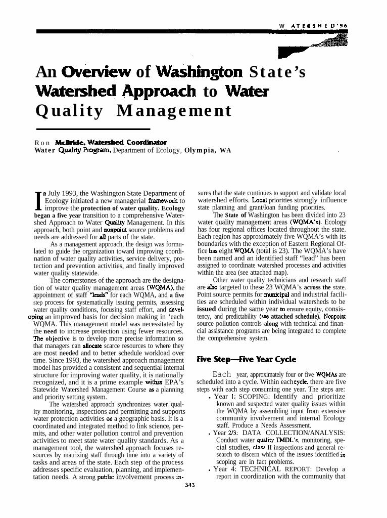
APPENDIX A

Washington State Department of Ecology:Watershed Approach to Water Quality Management

W A-f- E R 5 H E 0 ‘96

An overview of Wnshington State’sWaemhecf ApDmach to W&erQuality Management

R o n McBride, Watemhed CoordWorWater Quality Program, Department of Ecology, Olympia, WA .

In July 1993, the Washington State Department ofEcology initiated a new managerial tiamework toimprove the protection of water quality. Ecology

began a five year transition to a comprehensive Water-shed Approach to Water Quality Management. In thisapproach, both point and nonpoint source problems andneeds are addressed for all parts of the state.

As a management approach, the design was formu-lated to guide the organization toward improving coordi-nation of water quality activities, service delivery, pro-tection and prevention activities, and finally improvedwater quality statewide.

The cornerstones of the approach are the designa-tion of water quality management areas (WQMA), the

. appointment of staff “ieads” for each WQMA, and a fivestep process for systematically issuing permits, assessingwater quality conditions, focusing staff effort, and devel-

aping an improved basis for decision making in ‘eachWQMA. This management model was necessitated bythe need to increase protection using fewer resources.The objective is to develop more precise information sothat managers can allocate scarce resources to where theyare most needed and to better schedule workload overtime. Since 1993, the watershed approach managementmodel has provided a consistent and sequential internalstructure for improving water quality, it is nationallyrecognized, and it is a prime example wi,thin EPA’sStatewide Watershed Management Course as a planningand priority setting system.

The watershed approach synchronizes water qual-ity monitoring, inspections and permitting and supportswater protection activities ofi a geographic basis. It is acoordinated and integrated method to link science, per-mits, and other water pollution control and preventionactivities to meet state water quality standards. As amanagement tool, the watershed approach focuses re-sources by matrixing staff through time into a variety oftasks and areas of the state. Each step of the processaddresses specific evaluation, planning, and implemen-tation needs. A strong pubiic involvement process in-

sures that the state continues to support and validate localwatershed efforts. Local priorities strongly influencestate planning and grant/loan funding priorities.

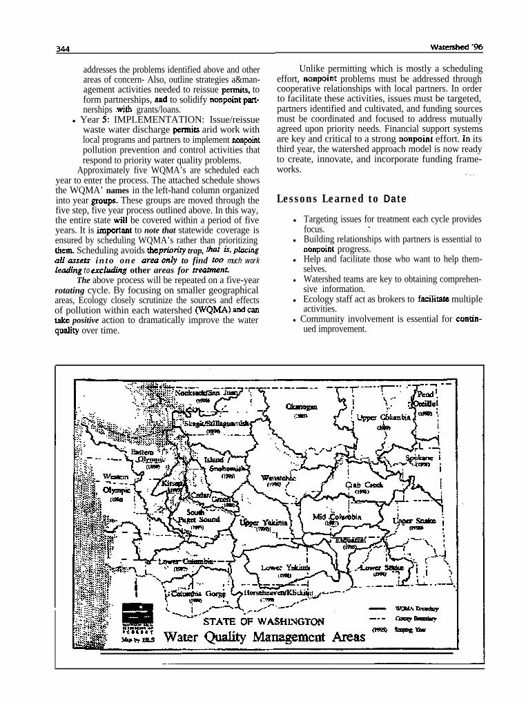
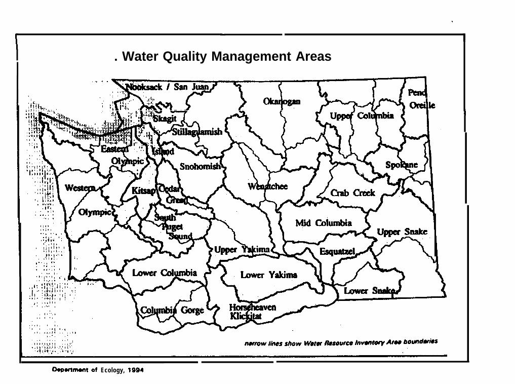
The State of Washington has been divided into 23water quality management areas (WQMA’s). Ecologyhas four regional offices located throughout the state.Each region has approximately five WQMA’s with itsboundaries with the exception of Eastern Regional Of-fice ha eight WQMA (total is 23). The WQMA’s havebeen named and an identified staff “lead” has beenassigned to coordinate watershed processes and activitieswithin the area (see attached map).

Other water quality technicians and research staffare aIso targeted to these 23 WQMA’s across the state.Point source permits for municipaf and industrial facili-ties are scheduled within individual watersheds to beissued during the same year to ensure equity, consis-tency, and predictability (see attached schedule). Nonpointsource pollution controls along with technical and finan-cial assistance programs are being integrated to completethe comprehensive system.

FiveStep-JiveYearCycle

Each year, approximately four or five WQMAs arescheduled into a cycle. Within each cycle, there are fivesteps with each step consuming one year. The steps are:

l Year I: SCOPING: Identify and prioritizeknown and suspected water quality issues withinthe WQMA by assembling input from extensivecommunity involvement and internal Ecologystaff. Produce a Needs Assessment.

l Year 2/3: DATA COLLECTION/ANALYSIS:Conduct water quality TMDL’s, monitoring, spe-cial studies, ciass II inspections and general re-search to discern which of the issues identified inscoping are in fact problems.

l Year 4: TECHNICAL REPORT: Develop areport in coordination with the community that

343

Watcfshed ‘%

addresses the problems identified above and otherareas of concern- Also, outline strategies a&man-agement activities needed to reissue permits, toform partnerships, and to solidify nonpoint part-nerships .with grants/loans.

l Year 5: IMPLEMENTATION: Issue/reissuewaste water discharge permits arid work withlocal programs and partners to implement nonpointpollution prevention and control activities thatrespond to priority water quality problems.

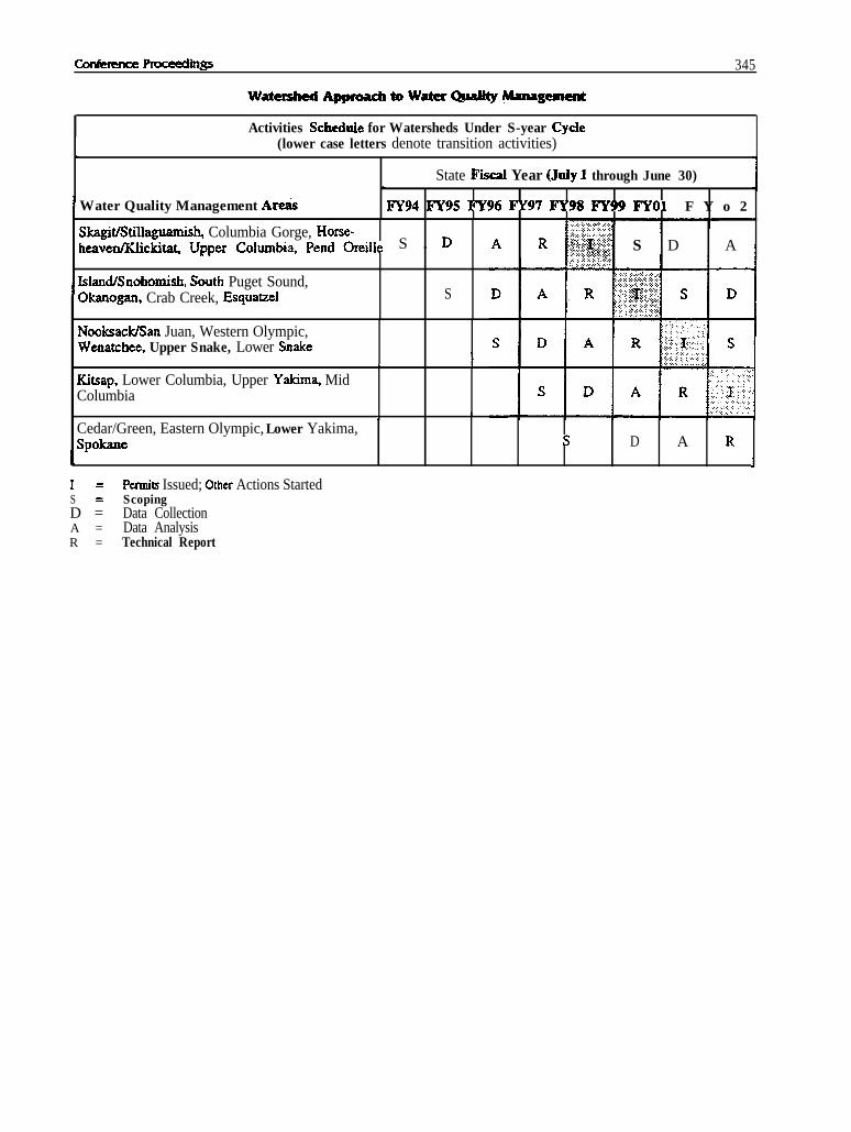
Approximately five WQMA’s are scheduled eachyear to enter the process. The attached schedule showsthe WQMA’ names in the left-hand column organizedinto year groups- These groups are moved through thefive step, five year process outlined above. In this way,the entire state will be covered within a period of fiveyears. It is important to note that statewide coverage isensured by scheduling WQMA’s rather than prioritizingthem. Scheduling avoids thepriority trap, that is, placingall ussets into one grea only to find too much workleading to e~cltbding other areas for treabnent-

The above process will be repeated on a five-yearrotating cycle. By focusing on smaller geographicalareas, Ecology closely scrutinize the sources and effectsof pollution within each watershed (‘WQMA) d cantie positive action to dramatically improve the water

Unlike permitting which is mostly a schedulingeffort, nonpoint problems must be addressed throughcooperative relationships with local partners. In orderto facilitate these activities, issues must be targeted,partners identified and cultivated, and funding sourcesmust be coordinated and focused to address mutuallyagreed upon priority needs. Financial support systemsare key and critical to a strong nonpoint effort. In itsthird year, the watershed approach model is now readyto create, innovate, and incorporate funding frame-works. . . .

.

Lessons Learned to Date

l Targeting issues for treatment each cycle providesfocus. .

l Building relationships with partners is essential tononpoint progress.

l Help and facilitate those who want to help them-selves.

l Watershed teams are key to obtaining comprehen-sive information.

l Ecology staff act as brokers to f&lit&e multipleactivities.

l Community involvement is essential for contin-quality over time. ued improvement.

Con- Pmceedins 345

Activities Schednie for Watersheds Under S-year Cycle(lower case letters denote transition activities)

State Fiscal Year (July 1 through June 30)

Water Quality Management Areis FY94 -95 FY96 Fy97 FY98 FY!w FYOI F Y o 2

SlcagitBtillaguamish, Columbia Gorge, Horse-haven/illi&tat, Upper Columbia, Pend Oreiile S . D A R S D A

IslandBnohomish, Souttr Puget Sound,Okanogan, Crab Creek, Esquatzel

Nooksack/San Juan, Western Olympic,Wenatchee, Upper Snake, Lower Sn&e

Kitsap, Lower Columbia, Upper Yakima, MidColumbia

S

\

1 f

ICedar/Green, Eastern Olympic, Lower Yakima,Spokane s D A R

1

I = Permits Issued; Othet Actions StartedS = ScopingD = Data CollectionA = Data AnalysisR = Technical Report

. Water Quality Management Areas

I .( *b .

. .

.

*.

lr-74-54k,

____ _bmnmnt of Ecology, 1994

APPENDIX B

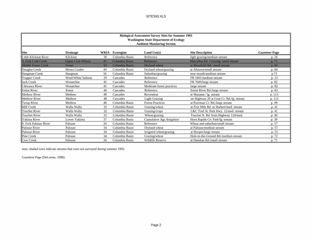
Site Locations of BiologicalAssessments in Washington State

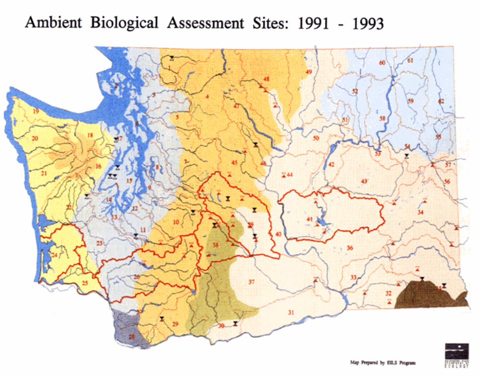
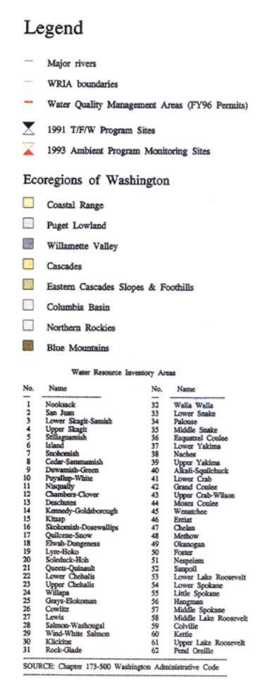
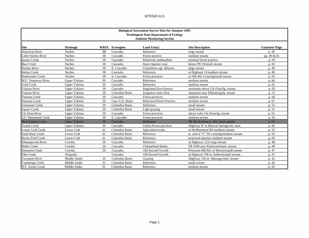
SITES93.XLS

Biological Assessment Survey Sites for Summer 1993Washington State Department of Ecology

Ambient Monitoring Section

Site Drainage WRIA Ecoregion Land Use(s) Site Description Gazetteer PageAmerican River Naches 38 Cascades Reference large stream p. 49Little Naches River Naches 38 Cascades Forest practice medium stream pp. 49 & 65Quartz Creek Naches 38 Cascades Relatively undisturbed minimal forest practice p. 65Bear Creek Naches 38 Cascades Intact riparian zone below FR 19/small stream p. 65Naches River Naches 38 E. Cascades Cumulative-agr. &forest. large stream p. 49Indian Creek Naches 38 Cascades Reference at Highway 12/medium stream p. 49Rattlesnake Creek Naches 38 E. Cascades Forest practices at Nile Rd. Crossing/small stream p. 50M.F. Teanaway River Upper Yakima 39 Cascades Reference medium stream p. 66Gold Creek Upper Yakima 39 Cascades Reference medium stream p. 65Yakima River Upper Yakima 39 Cascades Regulated flow/forestry mainstem above Cle Elum/lg. stream p. 65Yakima River Upper Yakima 39 Columbia Basin Irrigation return flow mainstem near Ellensburg/lg. stream p. 51Taneum Creek Upper Yakima 39 Cascades Forest practices medium stream p. 66Naneum Creek Upper Yakima 39 Casc./Col. Basin Reference/Forest Practice medium stream p. 67Umtanum Creek Upper Yakima 39 Columbia Basin Reference small stream p. 51Squaw Creek Upper Yakima 39 Columbia Basin Light grazing small stream p. 51Cle Elum River Upper Yakima 39 Cascades Forest practices above Lake Cle Elum/lg. stream p. 65S.F. Manastash Creek Upper Yakima 39 E. Cascades Forest practices medium stream p. 50Box Canyon Creek Upper Yakima 39 Cascades Reference FR 49; Kachess L. Rd./ med. stream p. 65Swauk Creek Upper Yakima 39 Cascades Utility/Forest practices Highway 97 at Mineral Springs/sm. strm. p. 66Lower Crab Creek Lower Crab 41 Columbia Basin Agriculture/crops at McManamon Rd./medium stream p. 53Sand Dune Creek Lower Crab 41 Columbia Basin Reference at end of "C" SE crossing/medium stream p. 53Rocky Ford Creek Lower Crab 41 Columbia Basin Reference protected riparian/ medium stream p. 69Ohanapecosh River Cowlitz 26 Cascades Reference at Highway 123/ large stream p. 48Butler Creek Cowlitz 26 Cascades Channelized Banks FR 5290 near Packwood/med. stream p. 48Simmons Creek Cowlitz 26 Cascades Old Second Growth Peterman Hill Rd. nr Morton/small stream p. 47Elbe Creek Nisqually Cascades Old Second Growth at Highway 706 nr Ashford/small stream p. 47Tucannon River Middle Snake 35 Columbia Basin Grazing Highway 126 nr. Mareago/med. stream p. 42Cummings Creek Middle Snake 35 Columbia Basin Reference small stream p. 42N.F. Asotin Creek Middle Snake 35 Columbia Basin Reference medium stream p. 43

Page 1

SITES93.XLS

Biological Assessment Survey Sites for Summer 1993Washington State Department of Ecology

Ambient Monitoring Section

Site Drainage WRIA Ecoregion Land Use(s) Site Description Gazetteer PageLittle Klickitat River Klickitat 30 Columbia Basin Reference light grazing/medium stream p. 26S. Fork Crab Creek Upper Crab-Wilson 43 Columbia Basin Reference Marcellus Rd. Crossing/ small stream p. 71Middle Foster Creek Foster 50 Columbia Basin Dryland wheat at Mansfield Rd./ small stream p. 84Douglas Creek Moses Coulee 44 Columbia Basin Dryland wheat/grazing at Alstown/small stream p. 84Hangman Creek Hangman 56 Columbia Basin Suburban/grazing near mouth/medium stream p.73Trapper Creek Wind-White Salmon 29 Cascades Reference FR 5401/medium stream p. 23Jack Creek Wenatchee 45 Cascades Reference FR 7600/large stream p. 82Chiwawa River Wenatchee 45 Cascades Moderate forest practices large stream p. 82Entiat River Entiat 46 Cascades Reference Entiat River Rd./large stream p. 83Methow River Methow 48 Cascades Recreation at Mazama / lg. stream p. 113Methow River Methow 48 Cascades Light Grazing on Highway 20 at Goat Cr. Rd./lg. stream p. 113Twisp River Methow 48 Columbia Basin Forest Practices at Poorman Cr. Rd./large stream p. 99Mill Creek Walla Walla 32 Columbia Basin Grazing/wheat at Five Mile Rd. nr Harbert/med. stream p. 41Touchet River Walla Walla 32 Columbia Basin Grazing/crops L&C Trail St. Park Hwy. 12/med. stream p. 41Touchet River Walla Walla 32 Columbia Basin Wheat/grazing Touchet N. Rd. from Highway 124/med. p. 40Yakima River Lower Yakima 37 Columbia Basin Cumulative Agr./Irrigation Horn Rapids Co. Park/lg. stream p. 39S. Fork Palouse River Palouse 34 Columbia Basin Reference Wheat and suburban/small stream p. 57Palouse River Palouse 34 Columbia Basin Dryland wheat at Palouse/medium stream p. 57Palouse River Palouse 34 Columbia Basin Irrigated wheat/grazing at Hooper/large stream p. 55Pine Creek Palouse 34 Columbia Basin Grazing/wheat Hole-in-the-Ground Rd./medium stream p. 72Cow Creek Palouse 34 Columbia Basin Wildlife Reserve at Danekas Rd./small stream p. 71

note: shaded rows indicate streams that were not surveyed during summer 1993.

Gazetteer Page (DeLorme, 1988)

Page 2

APPENDIX C

Field Forms for Chemical andPhysical Habitat Assessments

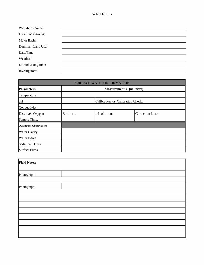
WATER.XLS

Waterbody Name:

Location/Station #:

Major Basin:

Dominant Land Use:

Date/Time:

Weather:

Latitude/Longitude:

Investigators:

SURFACE WATER INFORMATION

Parameters Measurement (Qualifiers)

Temperature

pH Calibration or Calibration Check:

Conductivity

Dissolved Oxygen Bottle no. mL of titrant Correction factor

Sample Time:

Qualitative Observations

Water Clarity

Water Odors

Sediment Odors

Surface Films

Field Notes:

Photograph:

Photograph:

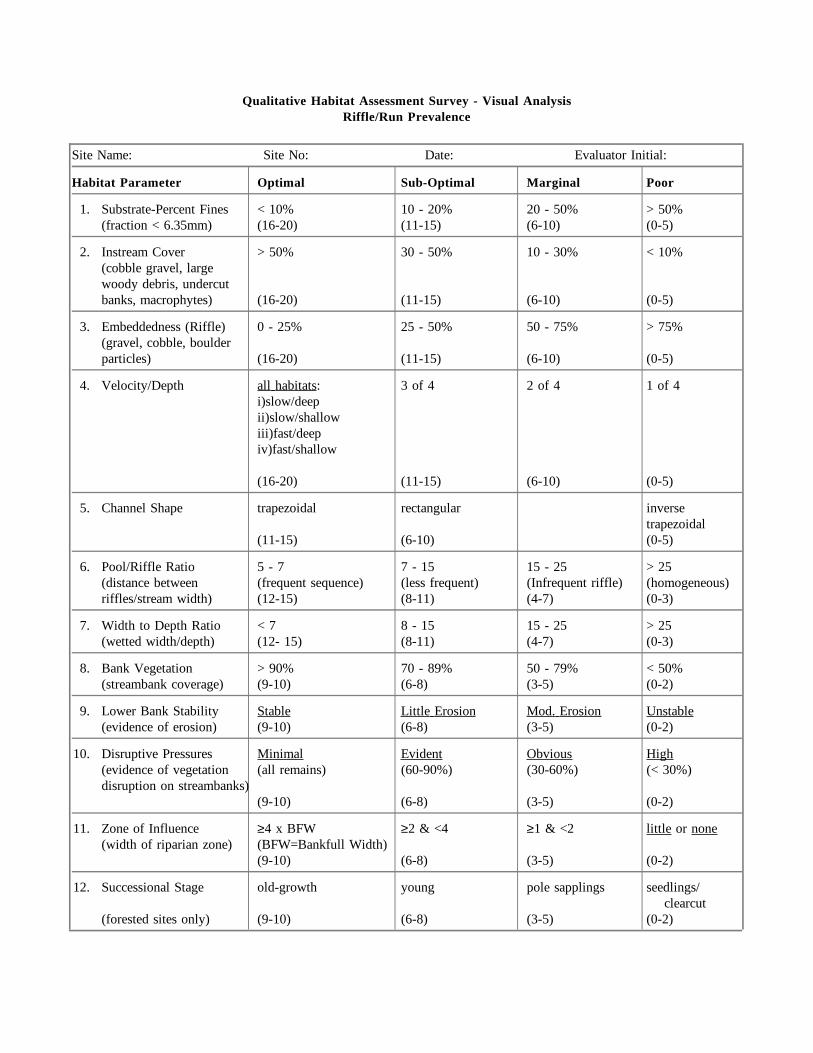
Qualitative Habitat Assessment Survey - Visual AnalysisRiffle/Run Prevalence

Site Name: Site No: Date: Evaluator Initial:

Habitat Parameter Optimal Sub-Optimal Marginal Poor

1. Substrate-Percent Fines < 10% 10 - 20% 20 - 50% > 50%(fraction < 6.35mm) (16-20) (11-15) (6-10) (0-5)

2. Instream Cover > 50% 30 - 50% 10 - 30% < 10%(cobble gravel, largewoody debris, undercutbanks, macrophytes) (16-20) (11-15) (6-10) (0-5)

3. Embeddedness (Riffle) 0 - 25% 25 - 50% 50 - 75% > 75%(gravel, cobble, boulderparticles) (16-20) (11-15) (6-10) (0-5)

4. Velocity/Depth all habitats: 3 of 4 2 of 4 1 of 4i)slow/deepii)slow/shallowiii)fast/deepiv)fast/shallow

(16-20) (11-15) (6-10) (0-5)

5. Channel Shape trapezoidal rectangular inversetrapezoidal

(11-15) (6-10) (0-5)

6. Pool/Riffle Ratio 5 - 7 7 - 15 15 - 25 > 25(distance between (frequent sequence) (less frequent) (Infrequent riffle) (homogeneous)riffles/stream width) (12-15) (8-11) (4-7) (0-3)

7. Width to Depth Ratio < 7 8 - 15 15 - 25 > 25(wetted width/depth) (12- 15) (8-11) (4-7) (0-3)

8. Bank Vegetation > 90% 70 - 89% 50 - 79% < 50%(streambank coverage) (9-10) (6-8) (3-5) (0-2)

9. Lower Bank Stability Stable Little Erosion Mod. Erosion Unstable(evidence of erosion) (9-10) (6-8) (3-5) (0-2)

10. Disruptive Pressures Minimal Evident Obvious High(evidence of vegetation (all remains) (60-90%) (30-60%) (< 30%)disruption on streambanks)

(9-10) (6-8) (3-5) (0-2)

11. Zone of Influence ≥4 x BFW ≥2 & <4 ≥1 & <2 little or none(width of riparian zone) (BFW=Bankfull Width)

(9-10) (6-8) (3-5) (0-2)

12. Successional Stage old-growth young pole sapplings seedlings/ clearcut

(forested sites only) (9-10) (6-8) (3-5) (0-2)

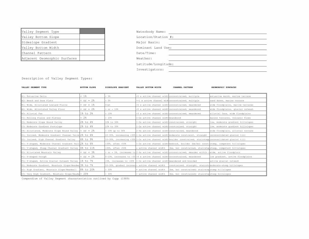
Valley Segment Type Waterbody Name:

Valley Bottom Slope Location/Station #:

Sideslope Gradient Major Basin:

Valley Bottom Width Dominant Land Use:

Channel Pattern Date/Time:

Adjacent Geomorphic Surfaces Weather:

Latitude/Longitude:

Investigators:

Description of Valley Segment Types:

VALLEY SEGMENT TYPE BOTTOM SLOPE SIDESLOPE GRADIENT VALLEY BOTTOM WIDTH CHANNEL PATTERN GEOMORPHIC SURFACES

A1: Estuarine Delta < 1% < 5% >5 x active channel widt hunconstrained, multiple estuarine marsh, marine terrace

A2: Beach and Dune Flats < or = 2% < 5% =>1 x active channel wid t unconstrained, multiple sand dunes, marine terrace

B1: Wide, Alluviated Lowland Plains < or = 1% flat >5 x active channel widt hunconstrained, meandered wide floodplains, marine terraces

B2: Wide, Alluviated Valley Floor < or = 2% > or = 10% >5 x active channel widt hunconstrained, meandered wide floodplains, glacial outwash

B3: Alluvial Fan 1% to 3% < 10% >3 x active channel widt hunconstrained, meandered alluvial fans, wide floodplains

C1: Rolling Plains and Plateau < 2% < 10% 1-2x active channel widt hmeandered marine terraces, volcanic flows

C2: Moderate Slope Bound Valley 2% to 4% 10% to 30% 1-2x active channel widt hconstrained, straight low, moderate gradient hillslopes

C3: Moderate Gradient Footslope 2% to 4% 10% to 30% 1-2x active channel widt hconstrained, straight low, moderate gradient hillslopes

C4: Alluviated, Moderate Slope Bound Valley < or = 2% < 10% up to 30% 2-4x active channel widt hconstrained, meandered wide floodplain, alluvial terrace

D1: Incised, Moderate Gradient Channel Valle y2% to 6% 10-30%, increasing >30% 1-2x active channel widt hmoderate constraint, straight unconsolidated glacial till

D2: Incised, High Channel Gradient Valley 6% to 9% 10-30%, increasing >30% 1-2x active channel widt hboulder constrained, stairstep punconsolidated glacial till

E1: V-shaped, Moderate Channel Gradient Vall e2% to 6% >30%, often >50% 1-2x active channel widt hbedrock, boulder (be/bo) const r steep, competent hillslopes

E2: V-shaped, Steep Channel Gradient Valley 6% to 11% >30%, often >50% = active channel width (be, bo) constrained, stairste psteep, competent hillslopes

E3: Alluviated Mountain Valley < or = 3% < or = 5%, increases to 2-4x active channel widt hunconstrained, meander within s wide, active floodplain

F1: U-shaped Trough < or = 2% 0-10%, increases to >30 %>4 x active channel widt hunconstrained, meandered low gradient, active floodplains

F2: U-shaped, Active Glacial Outwash Valley 1% to 7% <5%, increases to >30% 1-2x active channel widt hmeandered and braided active glacial outwash

G1: Moderate Gradient, Mountain Slope/Headwa t3% to 7% 10-30%, gradual increas e= active channel width constrained, straight, stairst emoderate-steep hillslopes

G2: High Gradient, Mountain Slope/Headwall 8% to 20% > 30% = active channel width (be, bo) constrained; stairste psteep hillslopes

G3: Very High Gradient, Mountain Slope/Headw a> 20% > 30% = active channel width (be, bo) constrained; stairste psteep hillslopes

Compendium of Valley Segment characteristics outlined by Cupp (1989)

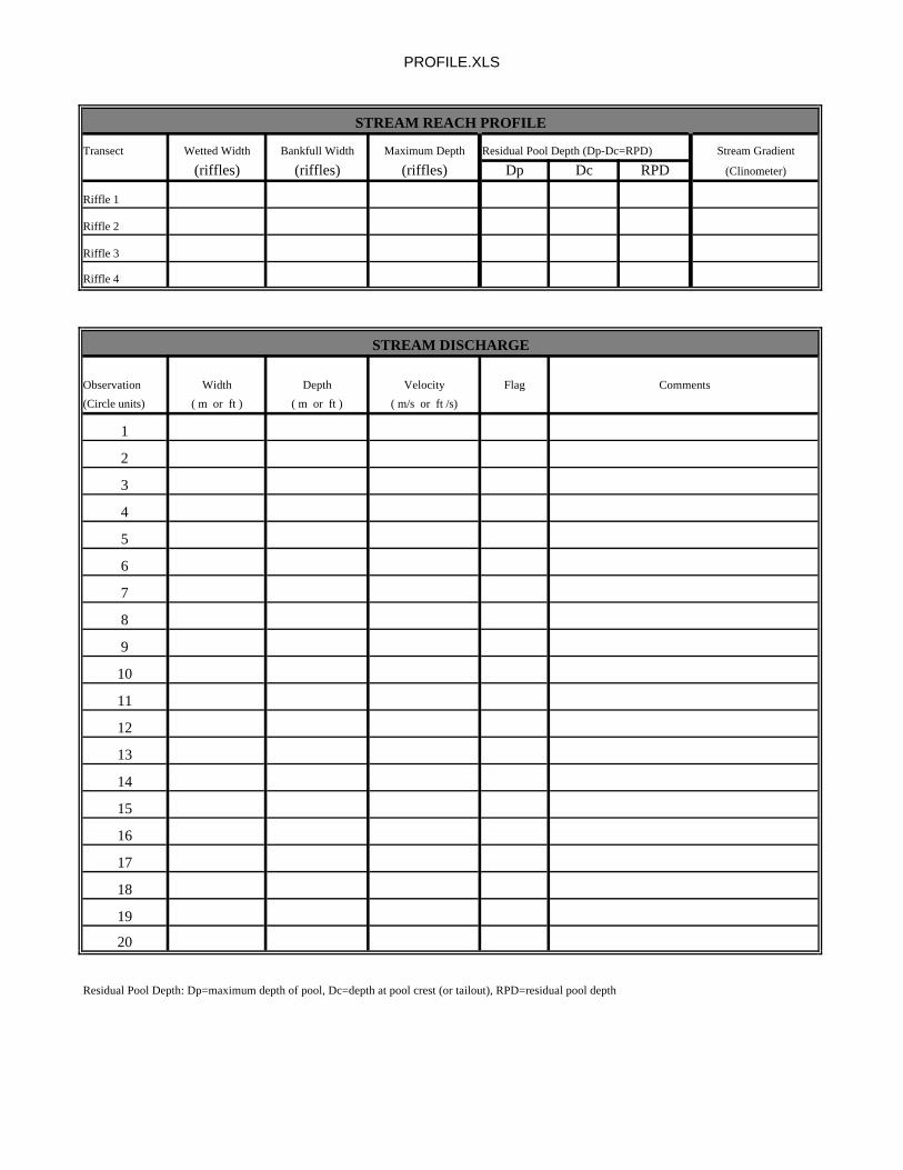
PROFILE.XLS

STREAM REACH PROFILE

Transect Wetted Width Bankfull Width Maximum Depth Residual Pool Depth (Dp-Dc=RPD) Stream Gradient

(riffles) (riffles) (riffles) Dp Dc RPD (Clinometer)

Riffle 1

Riffle 2

Riffle 3

Riffle 4

STREAM DISCHARGE

Observation Width Depth Velocity Flag Comments

(Circle units) ( m or ft ) ( m or ft ) ( m/s or ft /s)

1

2

3

4

5

6

7

8

9

10

11

12

13

14

15

16

17

18

19

20

Residual Pool Depth: Dp=maximum depth of pool, Dc=depth at pool crest (or tailout), RPD=residual pool depth

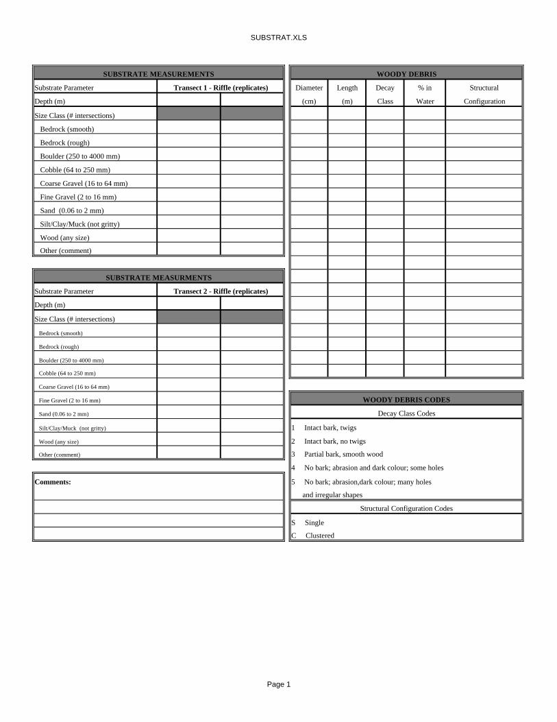
SUBSTRAT.XLS

SUBSTRATE MEASUREMENTS WOODY DEBRIS

Substrate Parameter Transect 1 - Riffle (replicates) Diameter Length Decay % in Structural

Depth (m) (cm) (m) Class Water Configuration

Size Class (# intersections)

Bedrock (smooth)

Bedrock (rough)

Boulder (250 to 4000 mm)

Cobble (64 to 250 mm)

Coarse Gravel (16 to 64 mm)

Fine Gravel (2 to 16 mm)

Sand (0.06 to 2 mm)

Silt/Clay/Muck (not gritty)

Wood (any size)

Other (comment)

SUBSTRATE MEASURMENTS

Substrate Parameter Transect 2 - Riffle (replicates)

Depth (m)

Size Class (# intersections)

Bedrock (smooth)

Bedrock (rough)

Boulder (250 to 4000 mm)

Cobble (64 to 250 mm)

Coarse Gravel (16 to 64 mm)

Fine Gravel (2 to 16 mm) WOODY DEBRIS CODES

Sand (0.06 to 2 mm) Decay Class Codes

Silt/Clay/Muck (not gritty) 1 Intact bark, twigs

Wood (any size) 2 Intact bark, no twigs

Other (comment) 3 Partial bark, smooth wood

4 No bark; abrasion and dark colour; some holes

Comments: 5 No bark; abrasion,dark colour; many holes

and irregular shapes

Structural Configuration Codes

S Single

C Clustered

Page 1

SUBEMBED.XLS

SUBSTRATE EMBEDDEDNESSDepth (total) / Depth (embedded) (Circle: cm or in.) Depth (total) / Depth (embedded) (Circle: cm or in.)

Transect 1 Transect 2

Page 1

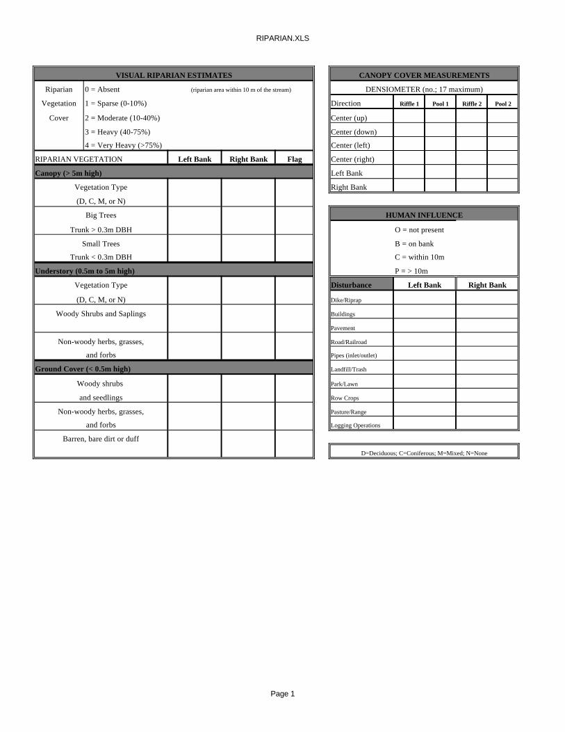
RIPARIAN.XLS

VISUAL RIPARIAN ESTIMATES CANOPY COVER MEASUREMENTS

Riparian 0 = Absent (riparian area within 10 m of the stream) DENSIOMETER (no.; 17 maximum)

Vegetation 1 = Sparse (0-10%) Direction Riffle 1 Pool 1 Riffle 2 Pool 2

Cover 2 = Moderate (10-40%) Center (up)

3 = Heavy (40-75%) Center (down)

4 = Very Heavy (>75%) Center (left)

RIPARIAN VEGETATION Left Bank Right Bank Flag Center (right)

Canopy (> 5m high) Left Bank

Vegetation Type Right Bank

(D, C, M, or N)

Big Trees HUMAN INFLUENCE

Trunk > 0.3m DBH O = not present

Small Trees B = on bank

Trunk < 0.3m DBH C = within 10m

Understory (0.5m to 5m high) P = > 10m

Vegetation Type Disturbance Left Bank Right Bank

(D, C, M, or N) Dike/Riprap

Woody Shrubs and Saplings Buildings

Pavement

Non-woody herbs, grasses, Road/Railroad

and forbs Pipes (inlet/outlet)

Ground Cover (< 0.5m high) Landfill/Trash

Woody shrubs Park/Lawn

and seedlings Row Crops

Non-woody herbs, grasses, Pasture/Range

and forbs Logging Operations

Barren, bare dirt or duff

D=Deciduous; C=Coniferous; M=Mixed; N=None

Page 1

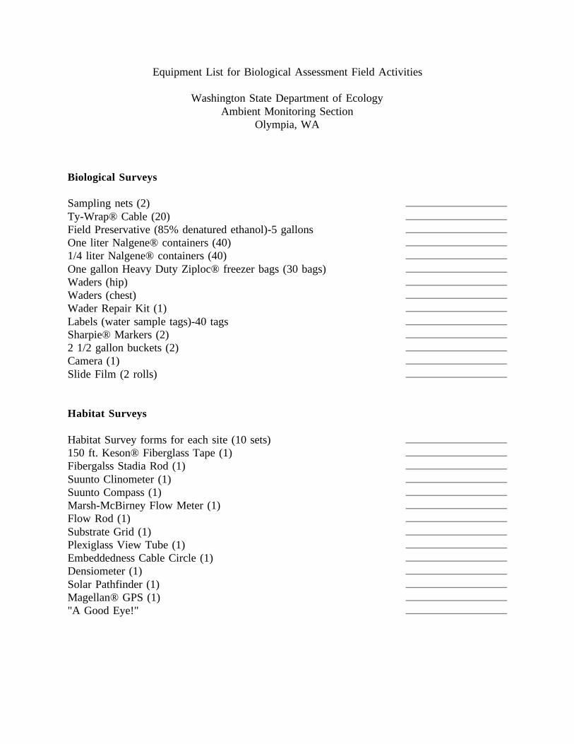
Equipment List for Biological Assessment Field Activities

Washington State Department of EcologyAmbient Monitoring Section

Olympia, WA

Biological Surveys

Sampling nets (2)Ty-Wrap® Cable (20)Field Preservative (85% denatured ethanol)-5 gallonsOne liter Nalgene® containers (40)1/4 liter Nalgene® containers (40)One gallon Heavy Duty Ziploc® freezer bags (30 bags)Waders (hip)Waders (chest)Wader Repair Kit (1)Labels (water sample tags)-40 tagsSharpie® Markers (2)2 1/2 gallon buckets (2)Camera (1)Slide Film (2 rolls)

Habitat Surveys

Habitat Survey forms for each site (10 sets)150 ft. Keson® Fiberglass Tape (1)Fibergalss Stadia Rod (1)Suunto Clinometer (1)Suunto Compass (1)Marsh-McBirney Flow Meter (1)Flow Rod (1)Substrate Grid (1)Plexiglass View Tube (1)Embeddedness Cable Circle (1)Densiometer (1)Solar Pathfinder (1)Magellan® GPS (1)"A Good Eye!"

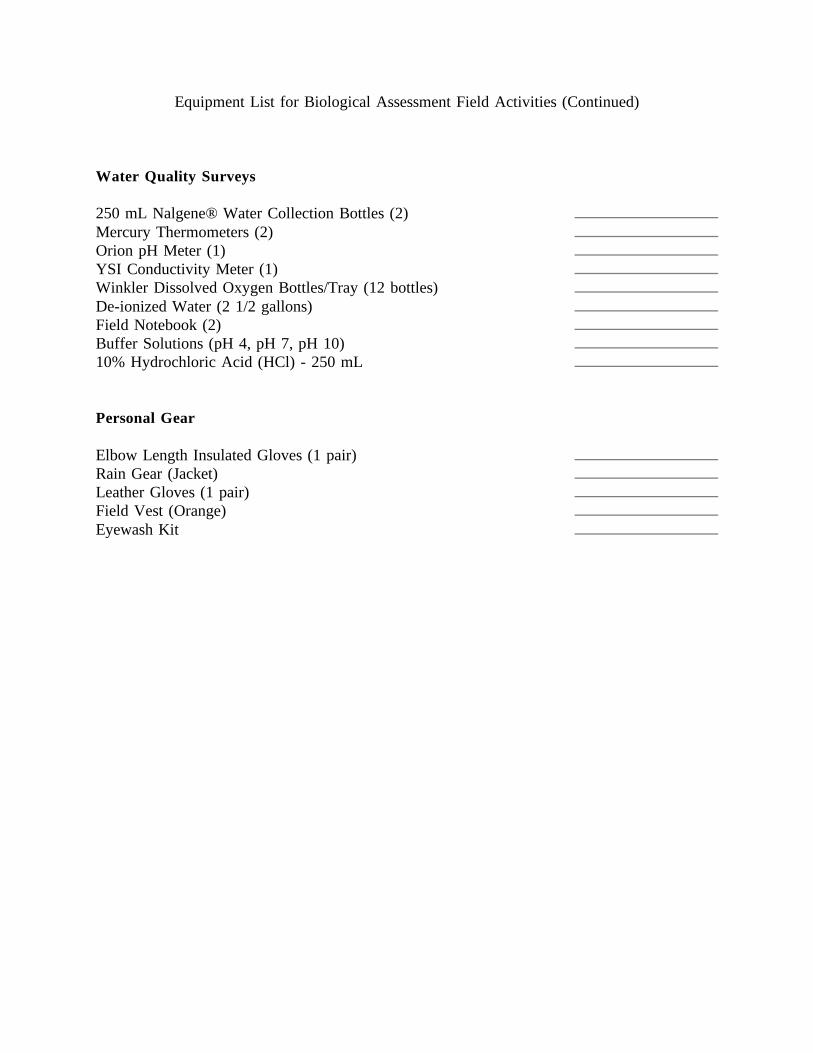
Equipment List for Biological Assessment Field Activities (Continued)

Water Quality Surveys

250 mL Nalgene® Water Collection Bottles (2)Mercury Thermometers (2)Orion pH Meter (1)YSI Conductivity Meter (1)Winkler Dissolved Oxygen Bottles/Tray (12 bottles)De-ionized Water (2 1/2 gallons)Field Notebook (2)Buffer Solutions (pH 4, pH 7, pH 10)10% Hydrochloric Acid (HCl) - 250 mL

Personal Gear

Elbow Length Insulated Gloves (1 pair)Rain Gear (Jacket)Leather Gloves (1 pair)Field Vest (Orange)Eyewash Kit

APPENDIX D

Data Management:Biological Information and Habitat Variables

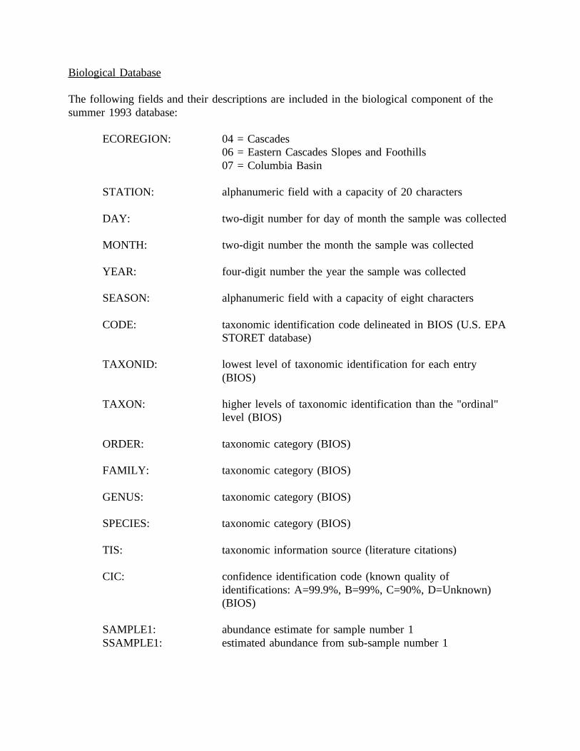
Biological Database

The following fields and their descriptions are included in the biological component of thesummer 1993 database:

ECOREGION: 04 = Cascades06 = Eastern Cascades Slopes and Foothills07 = Columbia Basin

STATION: alphanumeric field with a capacity of 20 characters

DAY: two-digit number for day of month the sample was collected

MONTH: two-digit number the month the sample was collected

YEAR: four-digit number the year the sample was collected

SEASON: alphanumeric field with a capacity of eight characters

CODE: taxonomic identification code delineated in BIOS (U.S. EPASTORET database)

TAXONID: lowest level of taxonomic identification for each entry(BIOS)

TAXON: higher levels of taxonomic identification than the "ordinal"level (BIOS)

ORDER: taxonomic category (BIOS)

FAMILY: taxonomic category (BIOS)

GENUS: taxonomic category (BIOS)

SPECIES: taxonomic category (BIOS)

TIS: taxonomic information source (literature citations)

CIC: confidence identification code (known quality ofidentifications: A=99.9%, B=99%, C=90%, D=Unknown)(BIOS)

SAMPLE1: abundance estimate for sample number 1SSAMPLE1: estimated abundance from sub-sample number 1

SAMPLE2: abundance estimate for replicate sampleSSAMPLE2: estimated abundance from replicate sub-sample

SAMPLE3: abundance estimate for replicate sampleSSAMPLE3: estimated abundance from replicate sub-sample

SAMPLE4: abundance estimate for replicate sampleSSAMPLE4: estimated abundance from replicate sub-sample

SAMPLE5: abundance estimate for replicate sampleSSAMPLE5: estimated abundance from replicate sub-sample

METHOD TYPE: HESS = modified Hess SamplerSURBER = Surber SamplerKICK = stationary square kicknetDKICK = stationary D-frame kicknetTRAVKICK = travelling D-frame kicknetROCK = multiple rock collection (usually three)PIBS = portable invertebrate box samplerECKMAN = Eckman GrabPONAR = Ponar GrabBASKET = wire mesh rock basket (artificial sampler)TRAY = rock-filled trays (artificial sampler)MPLATE = multi-plate artificial sampler

SAMPLE AREA: alphanumeric field that has an eight character capacity(examples of common notation: 1.0 m^2, 1.0 ft^2, 0.1 m^2,0.5 m^2)

FFG: functional feeding group classification of a taxon:

SHRED = Shredders (live plant or dead plant)CFILT = Collector-filterers (suspension feeders)CGATH = Collector-gatherers (deposit feeders)SCRAP = Scrapers (grazers)PREDT = Predators (engulfers)PIERC = Piercers (plant or animal)

TV: impact tolerance value of a taxon that is denoted byHilsenhoff (1977, 1982, 1987) and Plafkin et al. (1989).

STUDY: defines the type of site impact or anthropogenic influence, ifany:

REF = ReferenceAGR = Agricultural Practices

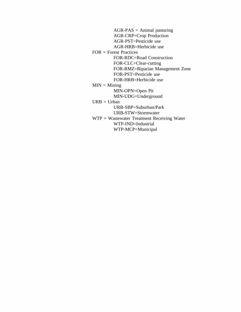
AGR-PAS = Animal pasturingAGR-CRP=Crop ProductionAGR-PST=Pesticide useAGR-HRB=Herbicide use

FOR = Forest PracticesFOR-RDC=Road ConstructionFOR-CLC=Clear-cuttingFOR-RMZ=Riparian Management ZoneFOR-PST=Pesticide useFOR-HRB=Herbicide use

MIN = MiningMIN-OPN=Open PitMIN-UDG=Underground

URB = UrbanURB-SBP=Suburban/ParkURB-STW=Stormwater

WTP = Wastewater Treatment Receiving WaterWTP-IND=IndustrialWTP-MCP=Municipal

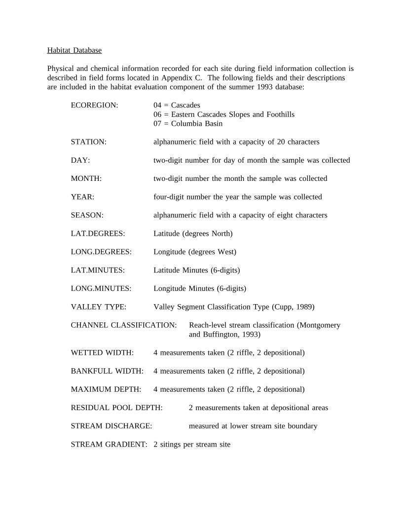
Habitat Database

Physical and chemical information recorded for each site during field information collection isdescribed in field forms located in Appendix C. The following fields and their descriptionsare included in the habitat evaluation component of the summer 1993 database:

ECOREGION: 04 = Cascades06 = Eastern Cascades Slopes and Foothills07 = Columbia Basin

STATION: alphanumeric field with a capacity of 20 characters

DAY: two-digit number for day of month the sample was collected

MONTH: two-digit number the month the sample was collected

YEAR: four-digit number the year the sample was collected

SEASON: alphanumeric field with a capacity of eight characters

LAT.DEGREES: Latitude (degrees North)

LONG.DEGREES: Longitude (degrees West)

LAT.MINUTES: Latitude Minutes (6-digits)

LONG.MINUTES: Longitude Minutes (6-digits)

VALLEY TYPE: Valley Segment Classification Type (Cupp, 1989)

CHANNEL CLASSIFICATION: Reach-level stream classification (Montgomeryand Buffington, 1993)

WETTED WIDTH: 4 measurements taken (2 riffle, 2 depositional)

BANKFULL WIDTH: 4 measurements taken (2 riffle, 2 depositional)

MAXIMUM DEPTH: 4 measurements taken (2 riffle, 2 depositional)

RESIDUAL POOL DEPTH: 2 measurements taken at depositional areas

STREAM DISCHARGE: measured at lower stream site boundary

STREAM GRADIENT: 2 sitings per stream site

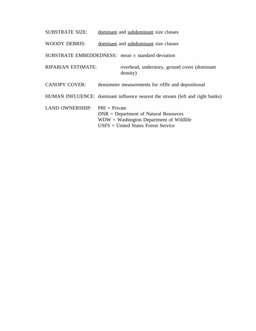
SUBSTRATE SIZE: dominant and subdominant size classes

WOODY DEBRIS: dominant and subdominant size classes

SUBSTRATE EMBEDDEDNESS: mean ± standard deviation

RIPARIAN ESTIMATE: overhead, understory, ground cover (dominantdensity)

CANOPY COVER: densimeter measurements for riffle and depositional

HUMAN INFLUENCE: dominant influence nearest the stream (left and right banks)

LAND OWNERSHIP: PRI = PrivateDNR = Department of Natural ResourcesWDW = Washington Department of WildlifeUSFS = United States Forest Service