Fall 2017

M. J. Prushan

CHL 311 Instrumental Analysis Lab Manual

1

Table of Content

CHM 311 Laboratory Schedule ................................................................................................................. 2

Instrumental Analysis Laboratory Policies ................................................................................................ 3

Instrumental Analysis Instrumentation Contract ..................................................................................... 5

MODULE I: SPECTRAL SOURCES AND SIGNAL TO NOISE

Experiment 1 BLACKBODY RADIATION or What’s the difference between a light bulb and the sun? ..... 10

Experiment 2 SPECTROSCOPY TRADING RULES: Signal-to-Noise, Resolution, Ensemble Averaging, Digital Smoothing ................................................................................................................................................... 12

MODULE II: SPECTROPHOTOMETERS: Instrumentation and Applications

Experiment 3 DETERMINATION OF CHLOROPHYLL IN OLIVE OIL by UV-Visible and Fluorescence

Spectroscopy .............................................................................................................................................. 17

Experiment 4 PERFORMANCE CHARACTERISTICS OF A SPECTROPHOTOMETER or Introduction to

Ultraviolet—Visible Spectrometry (UV-Vis) ................................................................................................ 22

Experiment 5 SPECTROPHOTOMETRIC ANALYSIS OF A MIXTURE, Determination of caffeine and benzoic acid in a soft drink ...................................................................................................................................... 32 Experiment 6 FLUORESCENCE Spectroscopy ............................................................................................. 36

MODULE III: CHROMATOGRAPHY

Experiment 7 QUALITATIVE GAS CHROMATOGRAPHY: The Van Deemter plot and optimum separation

Experiment 8 “IMPOSTER” vs. “REAL” PERFUMES via GC-MS ................................................................. 54

Experiment 9 DRUGS ON MONEY: GC-MS determination of cocaine on paper money ........................... 62

Appendix I INSTRUMENT INSTRUCTIONS .......................................................................................... 65

Appendix II USE OF A MICROSYRINGE FOR GC ................................................................................... 70

2

Instrumental Analysis Laboratory Policies INTRODUCTION In the laboratory portion of Instrumental Analysis you will be exposed to several different types of instrumental techniques. In most experiments, you will be investigating the performance characteristics of the instrument in addition to using it to make a measurement. It is still important, however, that you continue to use your best analytical technique when preparing standards and samples. Poor technique will always produce poor results! LABORATORY MODULES The laboratory course is divided into three modules, each of which emphasizes a different aspect of instrumental analysis. Each module consists of 2-4 experiments that relate to the theme of the module. You will work as part of a 2-person group, but because of limited instrument availability there is a possibility that you will have to schedule analysis time outside of class. LAB PREPARATION The key to efficiency in the lab is preparation. You are expected to read the lab and contact the instructor before the lab period for questions and/or clarifications. It is highly recommend that you consult with your group members before the lab period to divide responsibilities so that your laboratory time is used most efficiently. It is also important that you are considerate of your lab partners and arrive at lab on time. LAB NOTEBOOK You must keep a lab notebook starting with the first day of experiments. All data must be recorded in the laboratory notebook, not on loose sheets of paper or on the lab manual. To prevent abuse (i.e. filling in the notebook at the end of the semester), you must get the signature of the lab instructor each week. The primary purpose of the laboratory notebook is to record data and experimental details that are not included in the lab manual. You do not need to rewrite procedures that are already in the laboratory manual, and you do not need to include calculations. The notebook will be graded based on the following guidelines: 1. The first few pages of the notebook should be reserved for a table of contents. This table of contents should be kept up to date. 2. Each page should have a page number and be dated. 3. The notebook must be hard bound. 4. No pages should be removed for any reason. 5. All data entries must be in indelible (i.e. non-erasable) ink. 6. Mistakes and errors should be crossed out with a single line. White-out is not allowed. 7. Try to keep the notebook reasonably neat – you should be able to understand each entry. It is often helpful to construct tables prior to lab and fill them out as you collect data. 8. Keep your notebook current. It is unethical (not to mention illegal in many circumstances) to go back and fill in your notebook with data you wrote on loose pieces of paper. Backdating (i.e. going back and writing the date you think the data was recorded) is also forbidden.

3

REPORTS You must write a report (full, short or poster lab report) for each experiment. These reports are due one week after completing the lab.

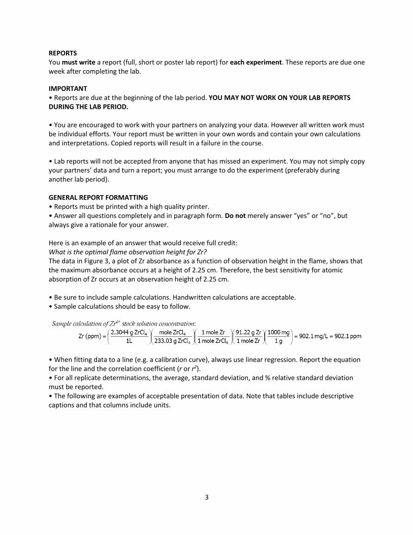
IMPORTANT • Reports are due at the beginning of the lab period. YOU MAY NOT WORK ON YOUR LAB REPORTS DURING THE LAB PERIOD. • You are encouraged to work with your partners on analyzing your data. However all written work must be individual efforts. Your report must be written in your own words and contain your own calculations and interpretations. Copied reports will result in a failure in the course. • Lab reports will not be accepted from anyone that has missed an experiment. You may not simply copy your partners’ data and turn a report; you must arrange to do the experiment (preferably during another lab period). GENERAL REPORT FORMATTING • Reports must be printed with a high quality printer. • Answer all questions completely and in paragraph form. Do not merely answer “yes” or “no”, but always give a rationale for your answer. Here is an example of an answer that would receive full credit: What is the optimal flame observation height for Zr? The data in Figure 3, a plot of Zr absorbance as a function of observation height in the flame, shows that the maximum absorbance occurs at a height of 2.25 cm. Therefore, the best sensitivity for atomic absorption of Zr occurs at an observation height of 2.25 cm. • Be sure to include sample calculations. Handwritten calculations are acceptable. • Sample calculations should be easy to follow.

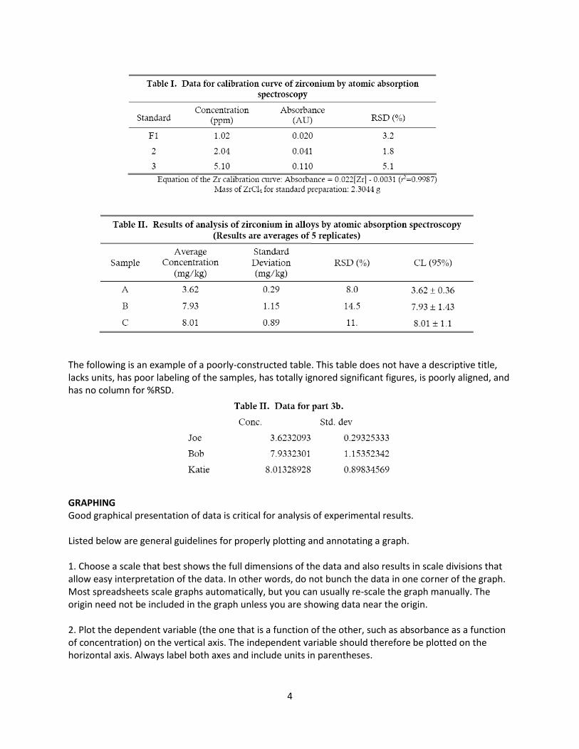
• When fitting data to a line (e.g. a calibration curve), always use linear regression. Report the equation for the line and the correlation coefficient (r or r2). • For all replicate determinations, the average, standard deviation, and % relative standard deviation must be reported. • The following are examples of acceptable presentation of data. Note that tables include descriptive captions and that columns include units.

4

The following is an example of a poorly-constructed table. This table does not have a descriptive title, lacks units, has poor labeling of the samples, has totally ignored significant figures, is poorly aligned, and has no column for %RSD.

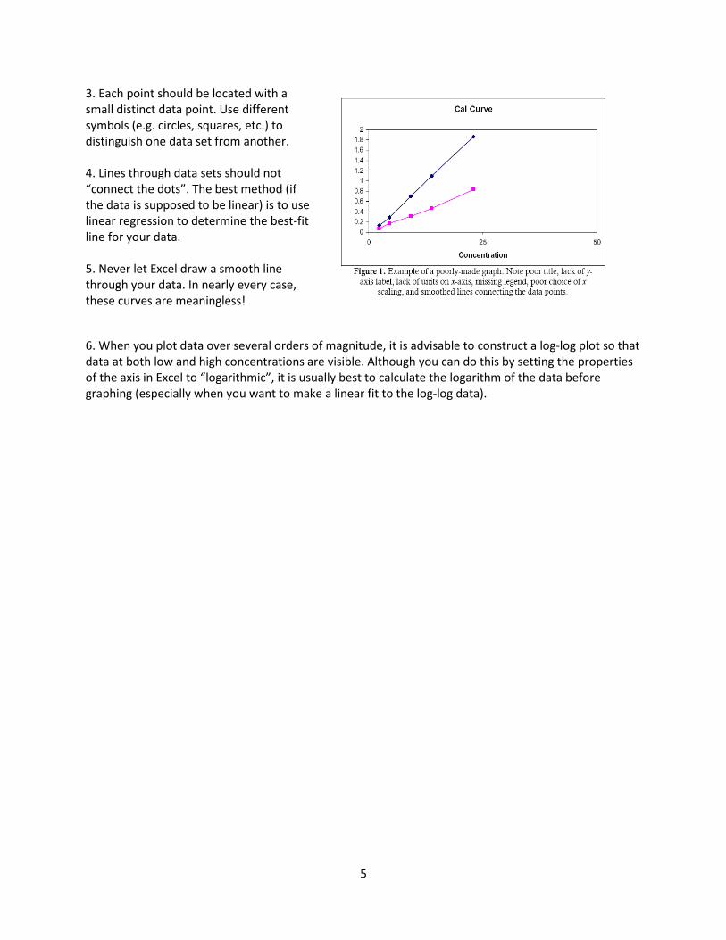
GRAPHING Good graphical presentation of data is critical for analysis of experimental results. Listed below are general guidelines for properly plotting and annotating a graph. 1. Choose a scale that best shows the full dimensions of the data and also results in scale divisions that allow easy interpretation of the data. In other words, do not bunch the data in one corner of the graph. Most spreadsheets scale graphs automatically, but you can usually re-scale the graph manually. The origin need not be included in the graph unless you are showing data near the origin. 2. Plot the dependent variable (the one that is a function of the other, such as absorbance as a function of concentration) on the vertical axis. The independent variable should therefore be plotted on the horizontal axis. Always label both axes and include units in parentheses.

5

3. Each point should be located with a small distinct data point. Use different symbols (e.g. circles, squares, etc.) to distinguish one data set from another. 4. Lines through data sets should not “connect the dots”. The best method (if the data is supposed to be linear) is to use linear regression to determine the best-fit line for your data. 5. Never let Excel draw a smooth line through your data. In nearly every case, these curves are meaningless!

6. When you plot data over several orders of magnitude, it is advisable to construct a log-log plot so that data at both low and high concentrations are visible. Although you can do this by setting the properties of the axis in Excel to “logarithmic”, it is usually best to calculate the logarithm of the data before graphing (especially when you want to make a linear fit to the log-log data).

6

[INSTRUCTOR COPY] CHL 311 Laboratory

Instrumentation Contract

The instrumental techniques that you will be learning are critical tools in so many areas of science, not

only in chemistry but also in medicine, geology, food science, forensic science, environmental and

agricultural science, material science, and pharmaceutical science as well. You will have a lot of

independence and opportunity to control your own work schedule. However, because of the structure

of the course, much of the responsibility for your education rests with you.

You will also have responsibility at times for the use and care of nearly $500,000 worth of

equipment. Often others will depend on your effort and cooperation. In order for everyone to get

the most out of this course and to protect you and the instrumentation we must agree to abide by

some rules.

Please read the following statements about expectations and use of facilities. Failure to follow

these rules will result in a failing grade in the course.

1. I will follow safe working procedures in lab. If the proper practice is unclear, or questionable in my

opinion, I will ask the instructor about it.

2. I agree not to eat or drink in the lab, nor to bring open beverages or containers of food into the lab. 3. I agree to clean up around the computers, lab benches and instruments whenever I work in the lab.

If I bring reagents, equipment or materials into the lab for my work, I will remove them when I leave for

the day.

4. I will see that the instrument or computer that I use is left in the appropriate idle (or off) condition

when I am done (unless the next user is present to take over).

5. I will sign the operator’s log book (if provided) after using an instrument and report any problems or

special needs (such as a low gas level) in the logbook or directly to the instructor.

6. Since equipment and supplies are intended for members of this class and other chemistry courses, I

will not remove any materials or equipment from the lab that I did not bring there without express

permission from a faculty member. (Obviously, such things as my data, print-outs and used reagents are

exceptions.)

7. I will not misuse any instruments or equipment in the lab.

8. I will not operate any equipment for which I have not been given instruction in operating.

9. I will be responsible for anyone that I let into the lab and will see that they abide by our class

guidelines for use of any equipment or facilities.

7

10. I will work through all of the reading assignments and tutorials.

11. I will cooperate with my lab partner. If the group becomes dysfunctional, it is part of my

responsibility to work things out. If that cannot be done satisfactorily in a short period of time, I will talk

to the instructor about the matter.

Signature _____________________________________

Date: ______________________

8

[STUDENT COPY] CHL 311 Laboratory

Instrumentation Contract

The instrumental techniques that you will be learning are critical tools in so many areas of science, not

only in chemistry but also in medicine, geology, food science, forensic science, environmental and

agricultural science, material science, and pharmaceutical science as well. You will have a lot of

independence and opportunity to control your own work schedule. However, because of the structure

of the course, much of the responsibility for your education rests with you.

You will also have responsibility at times for the use and care of nearly $500,000 worth of

equipment. Often others will depend on your effort and cooperation. In order for everyone to get

the most out of this course and to protect you and the instrumentation we must agree to abide by

some rules.

Please read the following statements about expectations and use of facilities. Failure to follow

these rules will result in a failing grade in the course.

1. I will follow safe working procedures in lab. If the proper practice is unclear, or questionable in my

opinion, I will ask the instructor about it.

2. I agree not to eat or drink in the lab, nor to bring open beverages or containers of food into the lab. 3. I agree to clean up around the computers, lab benches and instruments whenever I work in the lab.

If I bring reagents, equipment or materials into the lab for my work, I will remove them when I leave for

the day.

4. I will see that the instrument or computer that I use is left in the appropriate idle (or off) condition

when I am done (unless the next user is present to take over).

5. I will sign the operator’s log book (if provided) after using an instrument and report any problems or

special needs (such as a low gas level) in the logbook or directly to the instructor.

6. Since equipment and supplies are intended for members of this class and other chemistry courses, I

will not remove any materials or equipment from the lab that I did not bring there without express

permission from a faculty member. (Obviously, such things as my data, print-outs and used reagents are

exceptions.)

7. I will not misuse any instruments or equipment in the lab.

8. I will not operate any equipment for which I have not been given instruction in operating.

9. I will be responsible for anyone that I let into the lab and will see that they abide by our class

guidelines for use of any equipment or facilities.

9

10. I will work through all of the reading assignments and tutorials.

11. I will cooperate with my lab partner. If the group becomes dysfunctional, it is part of my

responsibility to work things out. If that cannot be done satisfactorily in a short period of time, I will talk

to the instructor about the matter.

Signature _____________________________________

Date: ______________________

10

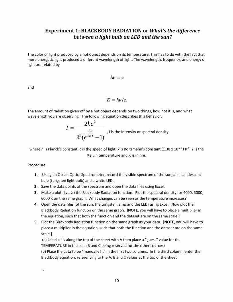
Experiment 1: BLACKBODY RADIATION or What’s the difference between a light bulb an LED and the sun?

The color of light produced by a hot object depends on its temperature. This has to do with the fact that more energetic light produced a different wavelength of light. The wavelength, frequency, and energy of light are related by

and

The amount of radiation given off by a hot object depends on two things, how hot it is, and what wavelength you are observing. The following equation describes this behavior.

)1(

2

5

2

kT

hc

e

hcI

, I is the Intensity or spectral density

where h is Planck’s constant, c is the speed of light, k is Boltzmann’s constant (1.38 x 10-23 J K-1) T is the

Kelvin temperature and is in nm.

Procedure.

1. Using an Ocean Optics Spectrometer, record the visible spectrum of the sun, an incandescent

bulb (tungsten light bulb) and a white LED.

2. Save the data points of the spectrum and open the data files using Excel.

3. Make a plot (I vs. ) the Blackbody Radiation function. Plot the spectral density for 4000, 5000,

6000 K on the same graph. What changes can be seen as the temperature increases?

4. Open the data files (of the sun, the tungsten lamp and the LED) using Excel. Now plot the

Blackbody Radiation function on the same graph. [NOTE, you will have to place a multiplier in

the equation, such that both the function and the dataset are on the same scale.]

5. Plot the Blackbody Radiation function on the same graph as your data. [NOTE, you will have to

place a multiplier in the equation, such that both the function and the dataset are on the same

scale.]

(a) Label cells along the top of the sheet with A then place a “guess” value for the

TEMPERATURE in the cell. (B and C being reserved for the other sources)

(b) Place the data to be “manually fit” in the first two columns. In the third column, enter the

Blackbody equation, referencing to the A, B and C values at the top of the sheet

.

11

6 . What temperature gives the best fit in each case? Look up values for the temperature of the

sun, the tungsten lamp and the LED, how do your experimental values compare?

7 Which of the two “give” off more visible light. What is the range of light that our eyes can see?

How does this overlap with the tungsten lamp, the LED and the sun spectra? Does this provide

evidence for why our eyes evolved to see particular wavelengths?

12

Experiment 2. SPECTROSCOPY TRADING RULES:

Signal-to-Noise, Resolution, Ensemble Averaging, Digital Smoothing

Introduction Using instrumentation of all kinds involves compromises. This lab is designed to illustrate some of the compromises involved in performing measurements with spectroscopic instrumentation: to demonstrate some of the “trading rules”. Before performing tasks illustrating these concepts, let's briefly discuss these terms, which you can read more about in the text. RESOLUTION: The most straight forward definition of resolution is in terms of the difference in frequency (wavenumber, cm-1) or wavelength (nm) between two absorbance peaks that can be just separated by the instrument. All other factors being equal, the greater the resolution the better to detect absorbances (peaks) as close together as possible. SIGNAL-TO-NOISE: In the text, S/N is defined as 1/RSD of a recorded signal. This can be thought of as the “root mean square” signal-to noise ratio. You will determine the rms S/N of the Fourier transform infrared spectrometer under a variety of instrumental conditions. All other factors being equal, the greater the S/N the better to detect the weakest absorbances, or absorbances at lower concentration levels. SIGNAL AVERAGING: Also called ensemble averaging, it's a way to enhance the S/N ratio by acquiring multiple spectra and obtaining the average of the result. The signal increases to the first power of the number of spectra averaged but the noise, being random, increases to the square root of the number of spectra averaged. Thus the signal increases faster than the noise as multiple spectra are averaged resulting in an increased signal-to-noise ratio. SMOOTHING: Also know as digital filtering (which is one way to smooth data that will be used in this laboratory). This is another way to enhance the S/N ratio of the spectrum. As you will see, there are trade-offs which must be considered when obtaining any spectrum. You always want a high S/N, but you need sufficient resolution to obtain a representative spectrum for your needs in a reasonable period of time. You must pick the appropriate conditions which best fulfill your needs, and the only way to accomplish this is to understand how S/N, spectral resolution, smoothing and signal averaging interact to change the data acquisition time and spectral result.

A Short Introduction to the Spectroscopy The absorption of electromagnetic radiation by ions and molecules serves as the basis for numerous analytical methods of analysis, both qualitative and quantitative. Studies of absorption spectra provide knowledge concerning the formula, structure, and stability of

13

many chemical species, as well as establish the most favorable conditions for analysis. Because the energy of a molecule is the sum of many individual types of energy, Emolecule = Eelectronic + Evibrational + Erotational + Etranslational + others absorption of a photon can increase molecular energy in a variety of ways. In UV-Visible spectroscopy, the energy of the photon corresponds with electronic energy transitions of molecules and ions. Thus UV-Visible spectroscopy is a type of electronic absorption spectroscopy. In infrared spectroscopy, the energy of the photon corresponds with vibrational energy levels of molecules. Thus infrared spectroscopy is a type of vibrational spectroscopy. It is usually safe to say that more detailed structural information can be derived from vibrational spectroscopy than from electronic spectroscopy. In UV-Vis electronic absorption spectroscopy in liquids, the absorption peaks are very broad. The broad peaks result from a phenomenon called “collisional broadening”. In the liquid state, molecules are contantly colliding and interacting with one another. This causes a near continuum of vibrational and rotational energy levels superimposed on top of the electronic energy levels; resulting in broad absorption bands over a range of wavelengths. These collisions are much less frequent in the gas phase, so one can see individual vibrational peaks superimposed on top of the electronic peaks in gas phase UV-Vis spectroscopy (assuming the instrumental conditions of obtaining the gas phase spectrum affords sufficient resolution). Similar phenomena occur in the infrared region, which is the part of the electromagnetic spectrum in which you will be working in this laboratory. Relatively broad peaks are observed in the infrared spectra of liquids, because a near continuum of rotational energies are superimposed on vibrational energy levels. Collisional broadening in the liquid phase makes it impossible to detect the individual rotational transitions. In the gas phase, you will see both vibrational and rotational transitions occurring as a series of sharp peaks. You will see this for gas phase CO2 in the atmosphere, and see changes in these gas phase spectra as you change the spectral resolution. You should conceptually understand what the implications are of spectral resolution in obtaining the gas phase spectra, and how the other variables of ensemble averaging, digital smoothing and resolution interact with one another to form some of the spectroscopic trading rules. Although we are using the FTIR spectrometer to illustrate the spectroscopy trading rules, it should be emphasized that any spectroscopic instrumentation will show the same types of trends. Since the FTIR is being used however, a few points which may otherwise cause confusion should be discussed. The FTIR is a single-beam instrument. The instrument components lab is designed to clearly show the difference between single-beam and double-beam instruments. A measurement of the % transmittance (from which absorbance can be calculated) actually requires 2 measurements.

%T = (I/Io) x 100

where I = intensity of light at a given wavelength that the detector senses when the sample is in the source beam, and Io = intensity of light at the same wavelength that the detector senses when a “blank” is in the source beam. In a single beam instrument an absorbance or % transmittance spectrum is obtained by first making measurements on a

14

blank to obtain Io as a function of wavelength or frequency. This is a single beam spectrum. Then a sample is put into the source beam and measurements obtained to obtain I as a function of wavelength or frequency. This is also a single beam spectrum. By taking the ratio of I/Io as a function of wavelength or frequency one obtains a transmittance spectrum. With the FTIR, when you collect a background spectrum, you obtain a plot of Io as a function of frequency. If you look at this spectrum you will see that the y-axis is not %T or absorbance, but emittance. This is simply a spectrum of instrument signal intensity as a function of frequency. When you obtain a sample spectrum, you obtain a plot of I as a function of frequency. You obtain a transmittance or absorbance spectrum by performing the appropriate mathematics to both I and Io. In this lab you collect both single beam spectra I and Io under identical conditions, that is no sample in the source beam in either case. In the resulting transmittance spectrum the deviation from 100%T is a direct measurement of the random error or noise of the measurement. In steps 6 and 7 of the procedure you are plotting single beam spectra of CO2, that is a plot of Io as a function of frequency. You are able to do this because of the CO2 in the air. Since what you are seeing here are single beam spectra, this is not a noise measurement (although noise always exists in the measurement). The differences you are seeing in steps 6 and 7 are primarily a result of differences that the instrument detects for the CO2 signal. Do not interpret the results in steps 6 and 7 as coming from differences in the amount of noise in the spectra. PROCEDURE 1. Your instructor will start up the Nicolet FTIR spectrometer, and briefly go over the operation of the instrument and the use of the software with you. You shouldn’t have to do anything with the instrument except type at the keyboard and plot spectra. Any questions or problems see the instructor. 2. With 1 scan, collect a background spectrum at 0.5 cm-1 resolution. With 1 scan, collect a sample spectrum at 0.5 cm-1 resolution. Find the S/N ratio of this spectrum between 2200 – 2000 cm-1. The Nicolet software will find the RMS noise within the displayed range for you. The S/N ratio is 100% T/RMS noise. Save this spectrum (100% T line) to disk. (Note: if your spectrometer’s software does not perform this calculation, students can manually obtain the peak-to-peak S/N ratio by taking 100 divided by the difference between the high and low points in the spectrum. 3. Now take this spectrum which you just calculated the S/N for, and perform a digital smoothing routine. First perform a 5 point smooth and calculate the S/N of this smoothed spectrum from 2200 – 2000 cm-1. Recall the unsmoothed spectrum and repeat the smoothing process using 9, 13, 17, 21 and 25 point smoothing routines. After each smoothing routine calculate the new S/N ratio and recall the unsmoothed spectrum. Tabulate your data and make

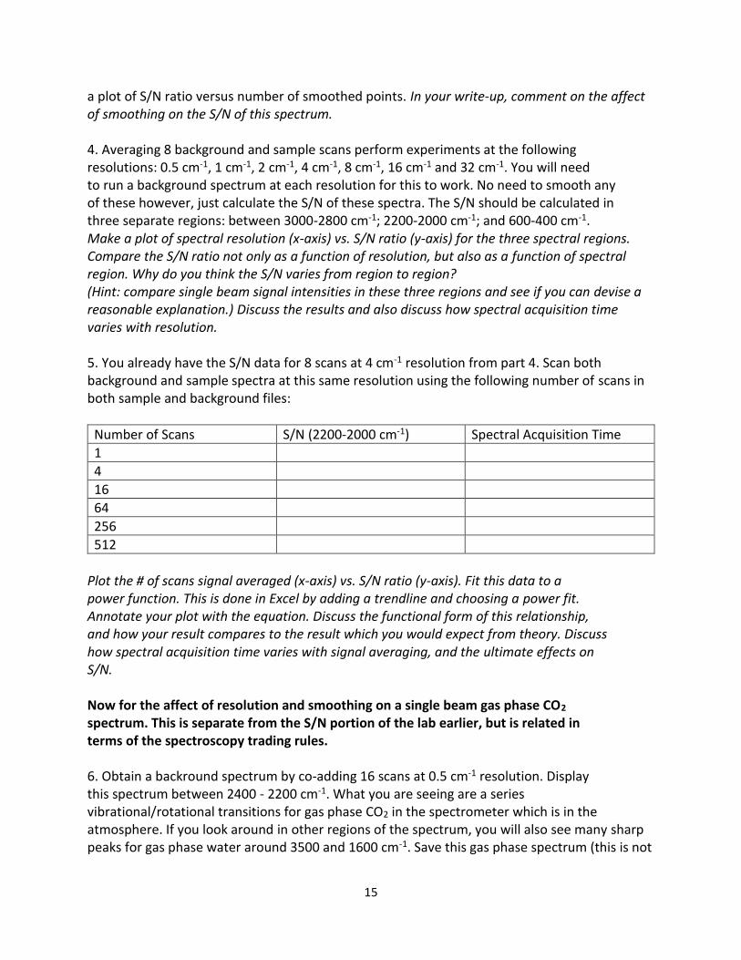
15

a plot of S/N ratio versus number of smoothed points. In your write-up, comment on the affect of smoothing on the S/N of this spectrum. 4. Averaging 8 background and sample scans perform experiments at the following resolutions: 0.5 cm-1, 1 cm-1, 2 cm-1, 4 cm-1, 8 cm-1, 16 cm-1 and 32 cm-1. You will need to run a background spectrum at each resolution for this to work. No need to smooth any of these however, just calculate the S/N of these spectra. The S/N should be calculated in three separate regions: between 3000-2800 cm-1; 2200-2000 cm-1; and 600-400 cm-1. Make a plot of spectral resolution (x-axis) vs. S/N ratio (y-axis) for the three spectral regions. Compare the S/N ratio not only as a function of resolution, but also as a function of spectral region. Why do you think the S/N varies from region to region? (Hint: compare single beam signal intensities in these three regions and see if you can devise a reasonable explanation.) Discuss the results and also discuss how spectral acquisition time varies with resolution. 5. You already have the S/N data for 8 scans at 4 cm-1 resolution from part 4. Scan both background and sample spectra at this same resolution using the following number of scans in both sample and background files:

Number of Scans S/N (2200-2000 cm-1) Spectral Acquisition Time

1

4

16

64

256

512

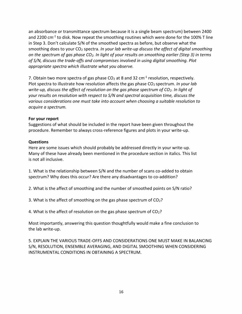
Plot the # of scans signal averaged (x-axis) vs. S/N ratio (y-axis). Fit this data to a power function. This is done in Excel by adding a trendline and choosing a power fit. Annotate your plot with the equation. Discuss the functional form of this relationship, and how your result compares to the result which you would expect from theory. Discuss how spectral acquisition time varies with signal averaging, and the ultimate effects on S/N. Now for the affect of resolution and smoothing on a single beam gas phase CO2 spectrum. This is separate from the S/N portion of the lab earlier, but is related in terms of the spectroscopy trading rules. 6. Obtain a backround spectrum by co-adding 16 scans at 0.5 cm-1 resolution. Display this spectrum between 2400 - 2200 cm-1. What you are seeing are a series vibrational/rotational transitions for gas phase CO2 in the spectrometer which is in the atmosphere. If you look around in other regions of the spectrum, you will also see many sharp peaks for gas phase water around 3500 and 1600 cm-1. Save this gas phase spectrum (this is not

16

an absorbance or transmittance spectrum because it is a single beam spectrum) between 2400 and 2200 cm-1 to disk. Now repeat the smoothing routines which were done for the 100% T line in Step 3. Don’t calculate S/N of the smoothed spectra as before, but observe what the smoothing does to your CO2 spectra. In your lab write-up discuss the affect of digital smoothing on the spectrum of gas phase CO2. In light of your results on smoothing earlier (Step 3) in terms of S/N, discuss the trade-offs and compromises involved in using digital smoothing. Plot appropriate spectra which illustrate what you observe. 7. Obtain two more spectra of gas phase CO2 at 8 and 32 cm-1 resolution, respectively. Plot spectra to illustrate how resolution affects the gas phase CO2 spectrum. In your lab write-up, discuss the affect of resolution on the gas phase spectrum of CO2. In light of your results on resolution with respect to S/N and spectral acquisition time, discuss the various considerations one must take into account when choosing a suitable resolution to acquire a spectrum. For your report Suggestions of what should be included in the report have been given throughout the procedure. Remember to always cross-reference figures and plots in your write-up. Questions Here are some issues which should probably be addressed directly in your write-up. Many of these have already been mentioned in the procedure section in italics. This list is not all inclusive. 1. What is the relationship between S/N and the number of scans co-added to obtain spectrum? Why does this occur? Are there any disadvantages to co-addition? 2. What is the affect of smoothing and the number of smoothed points on S/N ratio? 3. What is the affect of smoothing on the gas phase spectrum of CO2? 4. What is the affect of resolution on the gas phase spectrum of CO2? Most importantly, answering this question thoughtfully would make a fine conclusion to the lab write-up. 5. EXPLAIN THE VARIOUS TRADE-OFFS AND CONSIDERATIONS ONE MUST MAKE IN BALANCING S/N, RESOLUTION, ENSEMBLE AVERAGING, AND DIGITAL SMOOTHING WHEN CONSIDERING INSTRUMENTAL CONDITIONS IN OBTAINING A SPECTRUM.

17

Experiment 3.

Determination of Chlorophyll in Olive Oil by UV-Visible and Fluorescence Spectroscopies

Olive oil is made by pressing or extracting the rich oil from the olive fruit. It seems like a simple

matter to press the olives and collect the oil, but many oil extraction processes exist for the many

different types of olives grown around the world. To complicate things further, there are also various

grades of olive oil, and carefully selected groups of officials meet to define and redefine the grading of

olive oil. To help make our experiment a more scientific and less political exercise, we will winnow our

investigation of olive oil down to a manageable few variables. After processing, olive oil comes in three

common grades: extra virgin, regular, and light. Extra virgin olive oil is considered the highest quality. It

is the first pressing from freshly prepared olives. It has a greenish-yellow tint and a distinctively fruity

aroma because of the high levels of volatile materials extracted from the fruit. Regular olive oil is

collected with the help of a warm water slurry to increase yield, squeezing every last drop of oil out of

the olives. It is pale yellow in color, with a slight aroma, because it contains fewer volatile compounds.

Light olive oil is very light in color and has virtually no aroma because it has been processed under

pressure. This removes most of the chlorophyll and volatile compounds. Light olive oil is commonly used

for frying because it does not affect the taste of fried foods, and it is relatively inexpensive. The visible

light absorbance spectrum of chlorophyll gives interesting results. The chemistry of chlorophyll (some

references site four types: a, b, c, and d) creates absorbance peaks in the 400–500 nm range and in the

600–700 nm range. The combination of visible light that is not absorbed appears green to the human

eye, but different sources of chlorophylls will have different ratios of these peaks, which create various

shades of green. The ability of chlorophyll to soak up light energy across a wide swath of the visible

range helps power photosynthesis at optimum efficiency in plants. In this experiment, you will have two

primary goals. First, you will analyze the various grades of olive oil to determine the absorbance peaks

that are present and the relative amount of chlorophyll found in each grade. You will use a

Spectrometer to measure the absorbance of the olive oil samples over the visible light spectrum. You

will then test an unknown sample of olive oil and grade it as extra virgin, regular, or light.

OBJECTIVES In this experiment, you will:

Measure and analyze the visible light absorbance spectra of three standard olive oils: extra virgin, regular, and light.

Measure the absorbance spectrum of an “unknown” olive oil sample.

Identify the unknown olive oil as one of the three standard types.

Compare the results with those obtained via fluorescence spectroscopy

18

PROCEDURE 1. Connect the Spectrometer to the USB port of your computer. 2. Start Logger Pro. If it is already running, choose New from the File menu. 3. Obtain small volumes of the three standard and one unknown olive oils. Transfer enough of one olive oil sample to fill a cuvette 3/4 full. Place a lid on the cuvette and mark the lid. Prepare all of your samples in this way so that you have four cuvettes of olive oil with labeled lids. 4. Calibrate the Spectrometer.

a. Prepare a blank by filling an empty cuvette 3/4 full with distilled water. b. Choose Calibrate ► Spectrometer from the Experiment menu. c. When the warmup period is complete, place the blank in the Spectrometer. Make sure to align the cuvette so that the clear sides are facing the light source of the Spectrometer. d. Click Finish Calibration, and then click OK.

Part I Comparing Three Grades Of Olive Oil and Identifying an Unknown

For Part I of this experiment, you will calibrate the Spectrometer with distilled water. Your goals are: (1) to compare the absorbance spectra of the different grades of olive oil; and (2) to identify the grade of an unknown sample of olive oil. 5. Conduct a full spectrum analysis of an olive oil sample.

a. Place one of the olive oil samples in the Spectrometer. b. Click COLLECT. A full spectrum graph of the olive oil will be displayed. Review the graph to identify the peak absorbance values. Click STOP to complete the analysis.

6. To save your data, choose Store Latest Run from the Experiment menu. 7. Repeat Steps 5–6 with the remaining olive oil standard samples. 8. Repeat Step 5 with the unknown. Note: Do not store the last run. 9. Examine the plots of the olive oil samples. Save your experiment file. 10. Rinse and clean the cuvettes and other oil-bearing containers with isopropyl alcohol.

Part II Comparing the Chlorophyll Concentration of Regular and Extra Virgin Olive Oil In Part II, you will use the light grade of olive oil to calibrate the Spectrometer and presume that light olive oil contains no chlorophyll. Next, you will compare the chlorophyll content of the regular grade with the extra virgin grade. 11. Set up a new file and calibrate the Spectrometer using light olive oil.

a. Choose New from the File menu. b. Prepare a blank by filling an empty cuvette 3/4 full with light olive oil. c. Choose Calibrate ►Spectrometer from the Experiment menu.

19

d. When the warmup period is complete, place the light olive oil blank in the Spectrometer. Make sure to align the cuvette so that the clear sides are facing the light source of the Spectrometer e. Click “Finish Calibration”, and then click OK.

12. Measure the absorbance spectrum of regular and extra virgin olive oil. a. Remove the cuvette of light olive oil from the Spectrometer and replace it with the cuvette of regular olive oil. b. Click COLLECT. A full spectrum graph of the regular olive oil will be displayed. Note the slight difference in the plot as a result of using the light olive oil as the calibration blank. Click STOP. c. To save your data, choose Store Latest Run from the Experiment menu. d. Measure the absorbance spectrum of the extra virgin grade in the same way.

13. Save your experiment files.

Part III Fluorescence Spectroscopy of Chlorophyll in Olive Oil

Chlorophyll is a fluorescent molecule. Fluorescent molecules can absorb light of one wavelength and then reemit light at a new and longer wavelength of light. As you have seen in this experiment already, chlorophyll absorbs light in the violet and blue regions of the spectra. If you were to shine a violet or blue light through a sample of extra virgin olive oil, you would see the oil turn red in color. The intensity of the red color is an indication of how much chlorophyll is in the olive oil. 14. Shine the light from a UV Flashlight through a cuvette containing extra virgin olive oil. Does the sample that is hit by the light turn red in color? Repeat this test for regular olive oil, light olive oil, and your unknown. Could you use this method to determine if a sample of olive oil is really extra virgin olive oil? Could you use this method to determine the grade of any sample of olive oil? Fluorescence spectroscopy is another method that can be used to determine the quality of olive oil. In fluorescence spectroscopy, a sample can be “excited” with a chosen wavelength of light and the resulting fluorescence from the sample can be measured and quantified. The SpectroVis Plus from Vernier Software & Technology can be used for this purpose. 15. Follow the directions below to measure the fluorescence of all of your olive oil samples using the SpectroVis Plus.

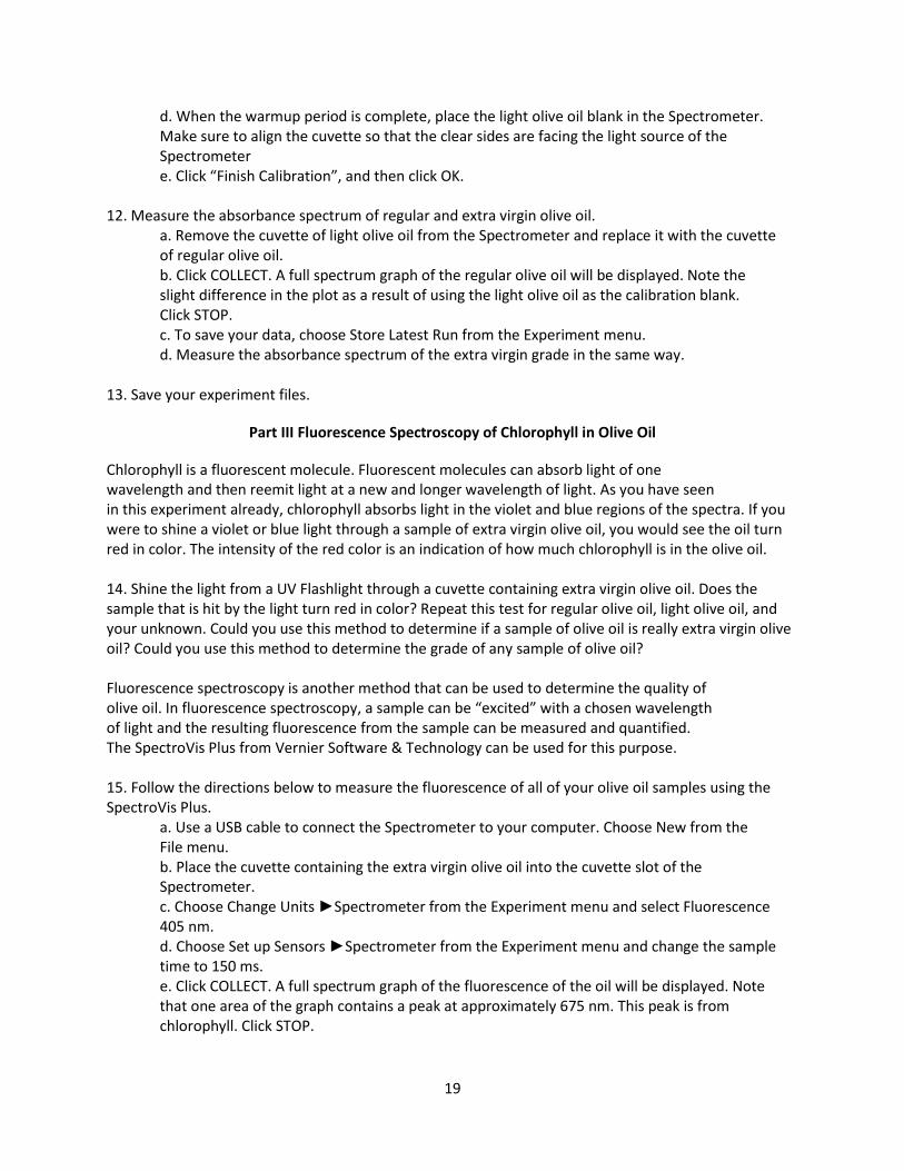
a. Use a USB cable to connect the Spectrometer to your computer. Choose New from the File menu. b. Place the cuvette containing the extra virgin olive oil into the cuvette slot of the Spectrometer. c. Choose Change Units ►Spectrometer from the Experiment menu and select Fluorescence 405 nm. d. Choose Set up Sensors ►Spectrometer from the Experiment menu and change the sample time to 150 ms. e. Click COLLECT. A full spectrum graph of the fluorescence of the oil will be displayed. Note that one area of the graph contains a peak at approximately 675 nm. This peak is from chlorophyll. Click STOP.

20

16. Adjust the sample time to increase or decrease the size of the fluorescent peak. If the peak intensity is above 1, decrease the sample time by 10 ms and collect a new fluorescent spectrum. Continue to decrease the sample time until the peak is fully visible. If the fluorescent peak is below 0.3, increase the sample time by 10 ms and collect a new fluorescent spectrum. Continue to increase the sample time until the peak fluorescent amplitude for the chlorophyll is above 0.8. 17. Once you have a nice peak, store your data by choosing Store Latest Run from the Experiment menu. 18. Collect full spectra from the remaining olive oil samples. Do not adjust the sample time. 19. Save your experiment files.

DATA ANALYSIS

Part I Comparing Three Grades of Olive Oil and Identifying an Unknown

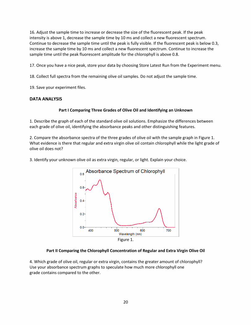
1. Describe the graph of each of the standard olive oil solutions. Emphasize the differences between each grade of olive oil, identifying the absorbance peaks and other distinguishing features. 2. Compare the absorbance spectra of the three grades of olive oil with the sample graph in Figure 1. What evidence is there that regular and extra virgin olive oil contain chlorophyll while the light grade of olive oil does not? 3. Identify your unknown olive oil as extra virgin, regular, or light. Explain your choice.

Figure 1.

Part II Comparing the Chlorophyll Concentration of Regular and Extra Virgin Olive Oil

4. Which grade of olive oil, regular or extra virgin, contains the greater amount of chlorophyll? Use your absorbance spectrum graphs to speculate how much more chlorophyll one grade contains compared to the other.

21

Part III Fluorescence Spectroscopy of Chlorophyll in Olive Oil

5. Compare the fluorescent spectra of the three grades of olive oil. The peak that is visible at approximately 675 nm is from chlorophyll. Which sample has the largest peak in this region? 6. Using the fluorescence from the known olive oil samples as your standards, determine the quality of your unknown olive oil sample. 7. Compare your results using fluorescent spectroscopy to your results using traditional spectroscopy. Is one method better than the other?

22

EXPERIMENT 4

PERFORMANCE CHARACTERISTICS OF A SPECTROPHOTOMETER or

Objective: Investigate several characteristics of a commercial spectrophotometer and compare different

cuvette materials.

Introduction: spectroscopy In this experiment you will become familiar with different features of

commercial ultraviolet-visible (UV/vis) spectrophotometers. The prefixes ultra and infra mean above

and below, respectively. Hence, the energy of ultraviolet radiation lies just above the visible violet light

(i.e., ultraviolet means above visible violet light in energy). Likewise, infrared means below visible red

light in energy. Because the energy range for a typical UV analysis is right next to the energy range of

visible light, many instruments, including ours, operate in both the UV and visible regions. In this lab

period, you will learn how to prepare samples for analysis and how to obtain data from the UV-Vis

instrument. The samples are compounds that might be found in explosives. They are nitroaromatics or

compounds that contain nitro groups (-NO2) bonded to an aromatic ring. In this case, the aromatic ring

is toluene. You will examine the output of the instrument in the wavelength region between 200 and

900 nm (nanometers). One nanometer is 1 x 10-9 meter. Background Theory for UV Absorption13 In

terms of energy, the IR region lies below the visible region, which lies below the UV region. Thus, IR is

strong enough to cause atoms within a molecule to vibrate, but not strong enough to cause electrons to

change orbital locations. UV radiation between 200 and 400 nm is strong enough to cause loosely held

electrons to change locations. These electrons can be either the non-bonding electrons (n-electrons) of

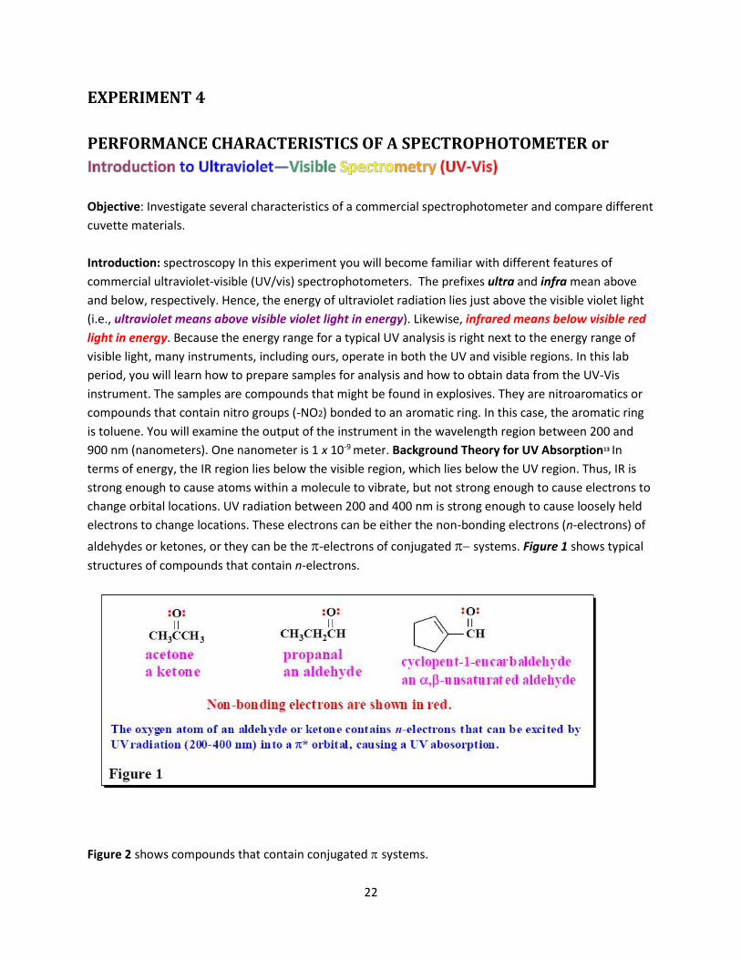
aldehydes or ketones, or they can be the -electrons of conjugated systems. Figure 1 shows typical

structures of compounds that contain n-electrons.

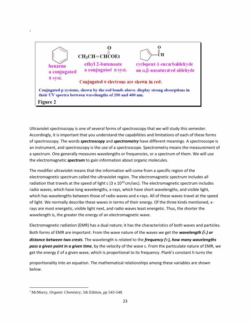
Figure 2 shows compounds that contain conjugated systems.

23

1

Ultraviolet spectroscopy is one of several forms of spectroscopy that we will study this semester.

Accordingly, it is important that you understand the capabilities and limitations of each of these forms

of spectroscopy. The words spectroscopy and spectrometry have different meanings. A spectroscope is

an instrument, and spectroscopy is the use of a spectroscope. Spectrometry means the measurement of

a spectrum. One generally measures wavelengths or frequencies, or a spectrum of them. We will use

the electromagnetic spectrum to gain information about organic molecules.

The modifier ultraviolet means that the information will come from a specific region of the

electromagnetic spectrum called the ultraviolet region. The electromagnetic spectrum includes all

radiation that travels at the speed of light c (3 x 1010 cm/sec). The electromagnetic spectrum includes

radio waves, which have long wavelengths, x-rays, which have short wavelengths, and visible light,

which has wavelengths between those of radio waves and x-rays. All of these waves travel at the speed

of light. We normally describe these waves in terms of their energy. Of the three kinds mentioned, x-

rays are most energetic, visible light next, and radio waves least energetic. Thus, the shorter the

wavelength is, the greater the energy of an electromagnetic wave.

Electromagnetic radiation (EMR) has a dual nature; it has the characteristics of both waves and particles.

Both forms of EMR are important. From the wave nature of the waves we get the wavelength () or

distance between two crests. The wavelength is related to the frequency (), how many wavelengths

pass a given point in a given time, by the velocity of the wave c. From the particulate nature of EMR, we

get the energy E of a given wave, which is proportional to its frequency. Plank’s constant h turns the

proportionality into an equation. The mathematical relationships among these variables are shown

below.

1 McMurry, Organic Chemistry, 5th Edition, pp 543-548.

24

Frequency and Wavelength: ν = c/λ or λ = c/ν or c = νλ

Energy and Frequency: E α ν or E = hν

Energy and Wavelength: E = hc/λ

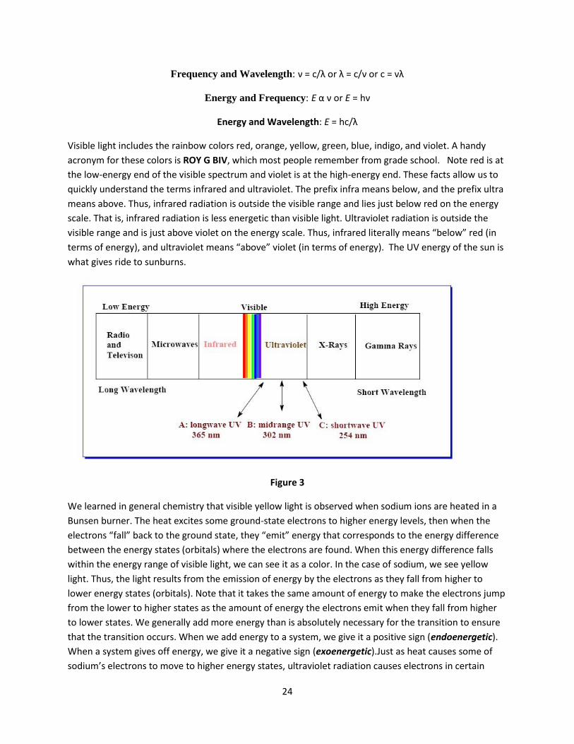
Visible light includes the rainbow colors red, orange, yellow, green, blue, indigo, and violet. A handy

acronym for these colors is ROY G BIV, which most people remember from grade school. Note red is at

the low-energy end of the visible spectrum and violet is at the high-energy end. These facts allow us to

quickly understand the terms infrared and ultraviolet. The prefix infra means below, and the prefix ultra

means above. Thus, infrared radiation is outside the visible range and lies just below red on the energy

scale. That is, infrared radiation is less energetic than visible light. Ultraviolet radiation is outside the

visible range and is just above violet on the energy scale. Thus, infrared literally means “below” red (in

terms of energy), and ultraviolet means “above” violet (in terms of energy). The UV energy of the sun is

what gives ride to sunburns.

Figure 3

We learned in general chemistry that visible yellow light is observed when sodium ions are heated in a

Bunsen burner. The heat excites some ground-state electrons to higher energy levels, then when the

electrons “fall” back to the ground state, they “emit” energy that corresponds to the energy difference

between the energy states (orbitals) where the electrons are found. When this energy difference falls

within the energy range of visible light, we can see it as a color. In the case of sodium, we see yellow

light. Thus, the light results from the emission of energy by the electrons as they fall from higher to

lower energy states (orbitals). Note that it takes the same amount of energy to make the electrons jump

from the lower to higher states as the amount of energy the electrons emit when they fall from higher

to lower states. We generally add more energy than is absolutely necessary for the transition to ensure

that the transition occurs. When we add energy to a system, we give it a positive sign (endoenergetic).

When a system gives off energy, we give it a negative sign (exoenergetic).Just as heat causes some of

sodium’s electrons to move to higher energy states, ultraviolet radiation causes electrons in certain

25

organic compounds to move from their ground state locations to orbitals of higher energy. The energy

of the ultraviolet light acts just like the energy of the heat. In this case, the molecules are said to

“absorb” ultraviolet radiation. A measurement of this phenomenon is called an absorption spectrum as

opposed to an emission spectrum. When electrons move from lower to higher energy levels, we call the

movement an electronic transition. Thus, the basic interaction between UV light and organic

compounds is that UV light causes electronic transitions in certain organic structures. That is, for a given

molecule, an electron changes orbital locations because the energy of the UV light forces it to change

locations.

The organic compound is dissolved in a solvent that does not absorb UV light. Such a solvent is said to

be transparent to UV light. The sample (compound in its solvent) is placed in a cuvette. A cuvette is a

sample holder that has very precise dimensions. The cuvette is placed in an ultraviolet

spectrophotometer. The instrument produces ultraviolet light over a range of wavelengths between 200

and 400 nanometers (nm), and the UV light is split into two equal beams. One beam is directed through

the solution of the organic compound (the sample) and the other beam is directed through the solvent

(the reference). The two beams are called the sample beam and the reference beam. A nanometer

equals a millimicron (mμ), which is sometimes still used by chemists to report wavelengths. As the UV

light passes through the sample, the instrument records a plot of absorbance (A) versus wavength (λ). In

other words, the instrument measures how much UV light is absorbed (the absorbance A) and where

the light is absorbed (the wavelength λ) for the specific sample. In this lab, we will obtain a UV spectrum

(plot of A vs. λ) for a sample of the organic compound toluene (methylbenzene) dissolved in hexane.

From the plot we will find the wavelength where the maximum absorbance occurs and record the

wavelength as λmax and the absorbance as a raw number. We call λmax the wavelength of maximum

absorbance. Thus, after you obtain your plot or printout of A vs. λ, all you will record on your data sheet

from the printout is λmax and A at λmax. We will then make use of certain relationships that govern how

much UV light can be absorbed by a sample. Namely, that the amount of light absorbed (A) is

proportional to how many molecules or the concentration (c) of molecules that are absorbing light, and

how far the UV light must pass through this concentration or the path length l. These relationships are

shown below.

A α c

A α l

A α c x l

This last proportionality says that the absorbance A is directly proportional to the concentration of the

sample and to the path length (width of the cuvette). This is why the dimensions of the cuvette must be

precise. The proportionality is useful for one given concentration or sample. A far more useful form of

the relationships above is the Beer-Lambert equation, which makes the proportionality into an equation

by addition of the proportionality constant ε (pronounced epsilon)

A = εcl

26

Beer-Lambert Equation

Like λ and ν, ε is a Greek letter. However, it is simply a constant that makes the above proportionality an

equation. The constant ε does not vary. So various concentrations of toluene measured in different size

cuvettes would give the same value of ε. Therefore, our laboratory exercise will include calculating ε.

The constant ε is called the molar extinction coefficient.

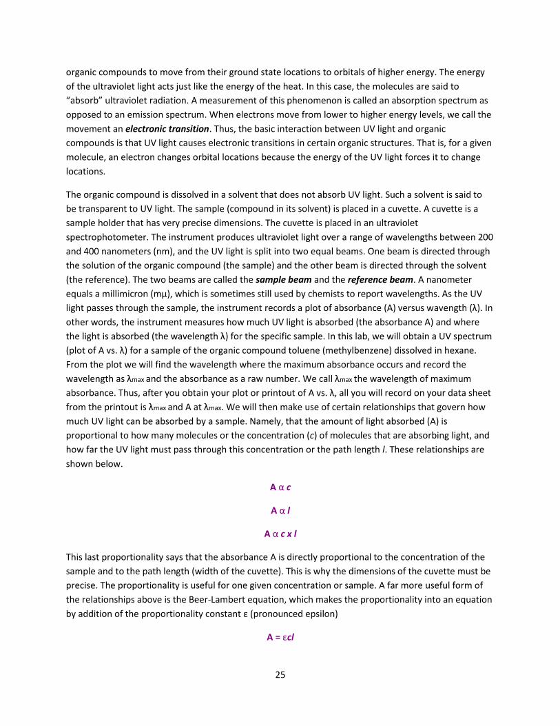
Therefore, the concentration of the sample must be in moles per liter (mol/L). The standard path length

is 1 cm. Thus, most cuvettes, including those in our lab, are exactly 1 cm wide where the light passes

through. These conventions ensure that everyone calculates ε the same way.

Figure 4. Cuvettes and Price List

We will learn that compounds such as benzene that contain conjugated π systems absorb UV light very

strongly (i.e., ε is typically 5,000 to 30,000). Whereas aldehyde and ketones, which contain isolated

carbonyl groups, absorb UV light weakly (i.e., ε is typically less than 100). The spectrum may be run on a

very small sample, but small amounts of impurities that absorb UV must be avoided.

Example problem: One milligram of a compound of molecular weight 140 is dissolved in 20 mL of

ethanol. The UV of the sample is measured in a 1-cm cuvette. The maximum absorption is 0.50 recorded

at 248 nm. Calculate the value of ε.

27

Solution: The concentration in mol/L = [(0.001)/140]mol/.012 L = 0.0060 mol/L ;

ε = A/cl = 0.50/(0.0060)(1.00) = 83.

Acids and acid derivatives, which contain a heteroatom next to the carbonyl might absorb UV radiation,

but not measurably in the 200-400 nm range. Therefore, except for aldehydes and ketones, compounds

that contain only carbonyl groups generally do not absorb UV radiation. Thus, UV spectroscopy enables

us to identify a conjugated π system or the carbonyl group of an aldehyde or ketone by the value we

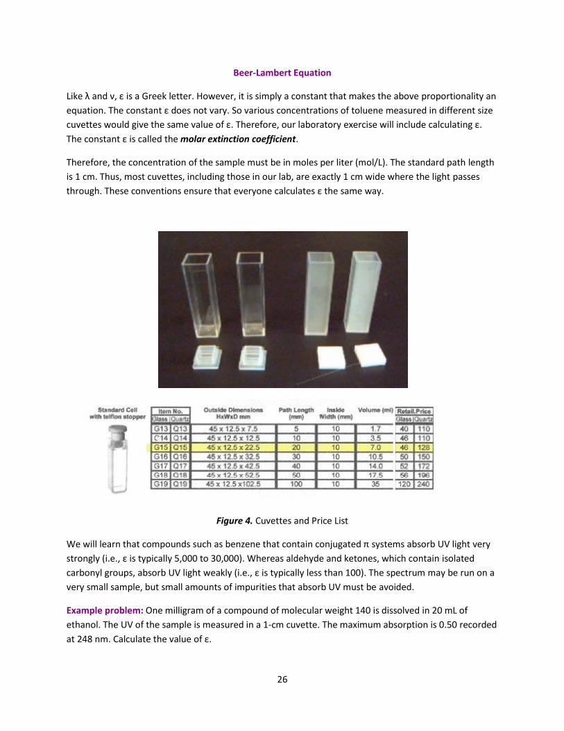
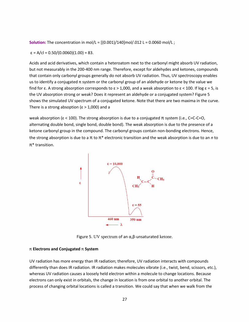
find for ε. A strong absorption corresponds to ε > 1,000, and a weak absorption to ε < 100. If log ε = 5, is

the UV absorption strong or weak? Does it represent an aldehyde or a conjugated system? Figure 5

shows the simulated UV spectrum of a conjugated ketone. Note that there are two maxima in the curve.

There is a strong absoption (ε > 1,000) and a

weak absorption (ε < 100). The strong absorption is due to a conjugated π system (i.e., C=C-C=O,

alternating double bond, single bond, double bond). The weak absorption is due to the presence of a

ketone carbonyl group in the compound. The carbonyl groups contain non-bonding electrons. Hence,

the strong absorption is due to a π to π* electronic transition and the weak absorption is due to an n to

π* transition.

Figure 5. UV spectrum of an α,β-unsaturated ketone.

π Electrons and Conjugated π System

UV radiation has more energy than IR radiation; therefore, UV radiation interacts with compounds

differently than does IR radiation. IR radiation makes molecules vibrate (i.e., twist, bend, scissors, etc.),

whereas UV radiation causes a loosely held electron within a molecule to change locations. Because

electrons can only exist in orbitals, the change in location is from one orbital to another orbital. The

process of changing orbital locations is called a transition. We could say that when we walk from the

28

first floor to the lab on the third floor that we transition to the lab, but the word transition is usually

reserved for the movement of a particle such as an electron from one orbital location to another. When

an electron changes orbital locations, we call the process an electronic transition. Electrons do not

change location spontaneously; they need help. The help appears in the form of UV radiation. UV

radiation is just energetic enough to cause certain loosely held electrons to move from one orbital to

another orbital but not energetic enough to cause an electron to be ejected from the molecule.

Radiation of higher energy than UV radiation such as X-ray or Gamma radiation is sufficiently energetic

to eject electrons. When a negatively-charged electron is ejected, a cation or positively-charged particle

is left. Therefore, high-energy radiation is called ionizing radiation. Of course, if a human is subjected to

ionizing radiation, the result can be a radiation injury. Thus, when you get a dental x-ray, a lead-

containing protective apron is draped over you to protect your body from the ionizing radiation.

The Instrument: See Quantitative Chemical Analysis, 6th Ed. Pg 462-463

You will perform checks on the following performance characteristics

• Wavelength calibration – How accurate are the reported wavelengths?

• Linearity – Is the photometric response linear over a reasonable absorption range?

• Resolution – How small of a wavelength difference can be detected?

• Effect of Slit Width – How does the exit slit of the monochromator affect the absorption spectrum?

Each of these is discussed in further detail below.

Wavelength Accuracy

The wavelength accuracy of a spectrophotometer is the correctness with which the wavelength of light

reaching the sample matches the wavelength reported by the instrument. When a wavelength is

selected, the monochromator’s grating (Grating 2 in Figure IB-1) is rotated so that the specified

wavelength is centered on the exit slit of the monochromator. Errors can come from two sources. First,

imperfections in the positioning system might cause errors in the grating rotation, which in turn causes

errors in the wavelength reaching the sample. Second, the light reaching the sample is not a single

wavelength, but rather a band of wavelengths. The width of this band is the spectral bandwidth (SBW)

of the instrument, and is defined as the width in nanometers of the band of light leaving the

monochromator measured halfway between the baseline and the peak intensity. Wavelength errors

tend to increase with SBW. Wavelength accuracy is verified using calibration standards. In general the

two standards that are used are theD2 source lamp lines and a holmium oxide (Ho2O3) filter. Both are

relatively stable and have several well-defined peak for calibration purposes. In this experiment we will

use the holmium oxide filter.

Resolution and the Effect of Spectral Bandwidth Resolution refers to the extent to which two peaks or bands (e.g., spectral, chromatographic, etc.) can be separated spatially such that peak overlap is minimized. The limiting resolution of the spectrophotometer depends upon the narrowest SBW that can be achieved. For high resolution work a very narrow SBW is required. A solution of toluene in hexane will be used to assess the resolution of the

29

instrument. The SBW of an instrument is a function of the exit slit width (w) and the reciprocal linear dispersion (D-1) of the monochromator. For a given value of D-1, the SBW is given by

SBW = wD−1 (4)

The reciprocal linear dispersion of a spectrophotometer is usually fixed, so SBW is controlled by changing the slit width. Using the spectrometer manual, determine D-1 in nm/mm and SBW range in nm. Smaller values of SBW (i.e. a smaller slit width) produce higher resolution spectra. But because the light intensity reaching the sample also decreases with slit width, spectra recorded with a small SBW also exhibit decreased signal-to-noise ratios. Conversely, larger values of SBW produce spectra with less noise (more light reaches the sample) but also with less resolution. The effect of SBW on the absorption spectrum of benzene vapor will be investigated as part of this experiment.

Safety Considerations. Benzene is a carcinogen. Do not open the cuvettes containing the benzene vapor.

Hexane and toluene are flammable and toxic.

Dispose of hexane, toluene in the appropriate waste container.

Procedure. This experimental procedure has several different parts, but they do not need to be done in sequentially.

Before using the instrument, prepare the following solutions. (Note that some of these will be provided for you; check with your instructor)

1. 0.020 %v/v Toluene in Hexane (UV grade) 2. 20-500 mM Ni2+, Co2+, or Cu2+ solutions (see introduction to Module I)

Have appropriate blanks ready for each solution.

Use quartz cuvettes for all components, unless otherwise noted.

NOTE: This procedure does NOT need to be performed every time you use the spectrophotometer.

However, it is important to realize that just because the readout from the instrument indicated that 500.00-

nm light is being measured, this does not absolutely guarantee that this is the case. If wavelength accuracy

is of primary concern, then you should verify the spectrophotometer’s calibration by measurement of the

absorption lines of holmium glass or emission lines of the deuterium (D2) lamp.

30

1. Wavelength Calibration, and Resolution

Holmium Glass Method. This method allows you to verify the wavelength calibration at three

different wavelengths, 460.0 nm, 360.9 nm and 279.4 nm. The performance is considered

satisfactory if the wavelength errors of the holmium glass absorption lines are within ±1 0.3 nm

a. With the Holmium Glass Filter in the sample compartment, record the spectrum

between 250 and 500 nm. at a 0.5 nm bandwidth, 10 nm/min scan speed, and a data

interval of 0.1 nm.

b. b) Determine the wavelengths of maximum absorbance using the Peak Pick Table. How

does the spectrum compare with the \wavelength values reported above?

Resolution. Record the spectrum of the toluene/hexane solution over the full range of the instrument

for a range of slit widths low to high. At what point can the “fine structure” no longer be seen? How is

this related to the resolution of the instrument?

2. Effect of slit width Place one drop of benzene in the bottom of a clean dry quartz cell and seal the cell. Do not get benzene on the walls of the cell. Put cell in the sample compartment; no reference is necessary. Set up the instrument to scan between 300 and 200 nm using a data interval of 0.200 nm (the scan rate should automatically adjust to 120 nm/min). Record the absorption spectrum of benzene vapor in the provided cuvette at spectral band widths (SBW) of 0.2, 0.5, 1.0, and 2.0 nm. Also record the spectrum using the Ocean Optics diode array spectrophotometer. Q1. What is the effect of spectral bandwidth on the absorption spectrum of benzene? Comment in terms of resolution and in terms of signal-to-noise ratio. Q2. Estimate the SBW for the diode array spectrophotometer by comparing the benzene spectrum to the spectra recorded at different SBW on the Unicam. Q3. When might a small SBW be necessary? When might a small SBW be a disadvantage?

3.Absorption properties of cuvette materials On a single graph, overlay spectra (recorded with the Unicam instrument over the entire uv-vis range) of cuvettes made of glass, plastic, and quartz. Leave the reference cuvet empty when recording this spectrum and use a reasonably fast scan rate (~700 nm/min). Also, be sure to record a blank spectrum (i.e. no cuvette in either holder). Include the overlaid spectra in the report. 4. Nitroaromatics.

a. Place the reference and sample cuvettes in the instrument in the correct locations.

b. Obtain the spectrum from 200-900 nm and save the data points of the spectrum. Note that our

instrument scans both visible and ultraviolet regions of the electromagnetic spectrum.

31

c. Repeat the procedure for using the other solutions of the nitroaromatic (in three solvents total)

For each of your nitroaromatic solutions , write out the appropriate UV data in the format you would

expect to see in a scientific journal (e.g., nitroaromatic: λmax 250 nm(ethanol), ε 12,000).

Determine whether the change in solvent resulted in a bathochromic, hypsochromic or no shift for the

nitroaromatic compound. (Show all spectra on the same graph, and clearly label). What conclusion(s)

can you draw from your data about the nature of the transitions in the compound?

Also to be include in the Report:

1. The report should contain a schematic diagram of the internal workings of the instrument.

2. For what types of molecules is UV-VIS spectroscopy most useful? For which is it not? As a

consequence, what are the best solvents for UV-VIS spectroscopy?

3. What is meant by bandwidth? As you narrow the bandwidth of the UV-VIS spectrometer, what might

you expect to happen to the spectrum?

4. Labeled copies of all the spectra and peak data.

5. Discuss in what situations would an accurate calibration of the UV-VIS be most important?

6. Discuss how changing the bandwidth changes the spectrum of the benzene vapor.

7. Compare the different optical material used to make cuvettes. What wavelength ranges is each

material useful for?

8. Explain what is meant by lambda max (λmax).

9. What information do you get from a molar extinction coefficient?

10. Draw the structure of cyclohexanone and show its non-bonding electrons. What value of ε do you

expect for cyclohexanone?

11. Draw a bond-line structure of toluene. What value of ε do you expect for toluene?

12. Why do the two examples in Figure 4 both have two maxima in their UV spectra?

13. A student dissolves 1.00 mg of a solid (140 g/mol) in 10.00 mL of ethanol. What is the concentration

of the solid in mol/L in the ethanolic solution?

14. One milligram of a compound of molecular weight 160 is dissolved in 10 mL of ethanol. The UV of

the sample is measured in a 1-cm cuvette. The maximum absorption is 0.60 recorded at 240 nm.

Calculate the value of ε.

15. Given a sample of acetophenone, predict what kind of UV spectrum you expect.

32

EXPERIMENT 5.

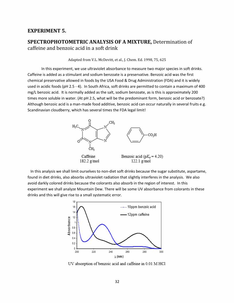
SPECTROPHOTOMETRIC ANALYSIS OF A MIXTURE, Determination of caffeine and benzoic acid in a soft drink

Adapted from V.L. McDevitt, et al., J. Chem. Ed. 1998, 75, 625

In this experiment, we use ultraviolet absorbance to measure two major species in soft drinks.

Caffeine is added as a stimulant and sodium benzoate is a preservative. Benzoic acid was the first

chemical preservative allowed in foods by the USA Food & Drug Administration (FDA) and it is widely

used in acidic foods (pH 2.5 - 4). In South Africa, soft drinks are permitted to contain a maximum of 400

mg/L benzoic acid. It is normally added as the salt, sodium benzoate, as is this is approximately 200

times more soluble in water. (At pH 2.5, what will be the predominant form, benzoic acid or benzoate?)

Although benzoic acid is a man-made food additive, benzoic acid can occur naturally in several fruits e.g.

Scandinavian cloudberry, which has several times the FDA legal limit!

In this analysis we shall limit ourselves to non-diet soft drinks because the sugar substitute, aspartame,

found in diet drinks, also absorbs ultraviolet radiation that slightly interferes in the analysis. We also

avoid darkly colored drinks because the colorants also absorb in the region of interest. In this

experiment we shall analyze Mountain Dew. There will be some UV absorbance from colorants in these

drinks and this will give rise to a small systematic error.

33

Beer’s law also applies to a medium containing more than one kind of absorbing substance. Provided

there is no interaction among the various species, the total absorbance for a multicomponent system is

given by: A total = A1 + A2 + .….. + An (Equation 1)

A total = 1bc1 + 2bc2 + .….. + nbcn

where the subscripts refer to absorbing components 1, 2, …n.

The above equation indicates that the total absorbance of a solution at a given wavelength is equal to

the sum of the absorbances of the individual components present. This relationship makes possible the

quantitative determination of the individual constituents of a mixture, even if their spectra overlap. If

enough spectrometric information is available, all of the components of mixtures can be quantified

without separation. For a two-component mixture (compound X and Y) with overlapping absorbances,

one could solve for the concentration of each species, [X] and [Y], by measuring the absorbances at two

different wavelengths, λ' and λ". The problem is mathematically equivalent to having two simultaneous

equations with two unknowns.

A1= X,1 bcX + Y,1 bcy (total absorbance at λ') (Equation 2)

A2= x,2 bcx + y,2 bcy (total absorbance at λ") (Equation 3)

The four molar absorptivities, X,1, Y,1 ,x,2, y,2 , can be evaluated from individual standard solutions of

X and Y, or better, from the slopes of their Beer’s law plots. The problem becomes simpler when one of

the compounds has no interference with the other compound. If there is substantial interference then

you must solve the simultaneous equations. Using UV spectroscopy, you will determine the

concentrations of caffeine and sodium benzoate (determined as benzoic acid), in the soft drink

Mountain Dew. The UV spectra of caffeine and benzoic acid overlap at certain wavelengths, thus you

will need to measure the absorbance of the unknown mixtures using two different wavelengths, and

apply equations 2 and 3 to evaluate the concentrations of caffeine and benzoic acid. See your textbook

for help in carrying out the calculations. The experiment could be shortened by recording just one

spectrum of caffeine (20 mg/L) and one of benzoic acid (10 mg/L) and assuming that Beer’s law is

obeyed. However, we shall construct a calibration graph and carry out a full analysis. Are there

advantages for doing this? If yes, please explain.

Reagents Stock solutions: benzoic acid 100 mg /L; caffeine 200 mg /L and 0.10 M HCl

34

Procedure

1. Calibration standards: Prepare a set of benzoic acid solutions containing 2, 4, 6, 8, and 10 mg/L in

0.010 M HCl. In a similar manner, prepare caffeine standards containing 4, 8, 12, 16, and 20 mg/L in

0.010 M HCl.

2. Soft drink: Warm ~ 20 mL of soft drink in a beaker on a hot plate to expel CO2 and filter the warm

liquid through filter paper to remove any particles. After cooling to room temperature, pipette 2.00 mL

into a 50-mL volumetric flask. Add 10.0 mL of 0.10 M HCl and dilute to the mark.

3. Verifying Beer’s law: Record the ultraviolet spectrum of each of the 10 standards with water in the

reference cuvette. Note the wavelength of peak absorbance for benzoic acid (λ′) and the wavelength for

the peak absorbance of caffeine (λ′′). Measure the absorbance of each standard at both wavelengths.

Prepare a calibration graph of absorbance versus concentration for each compound at each of the two

wavelengths. Each graph should go through 0. The slope of the graph is the absorptivity at that

wavelength.

4. Unknowns: Measure the ultraviolet absorption spectrum of the diluted sample of the soft drink.

With the absorbance at the wavelengths λ′ and λ′′ determine the concentrations of benzoic acid and

caffeine in the original soft drink.

5. You will need to save the data to flash drive so that you can copy the data from the spectrometers in

the form of a .csv file. This can then be converted using Microsoft Excel into a UV spectrum.

35

EXPERIMENT 5

FLUORESCENCE SPECTROSCOPY

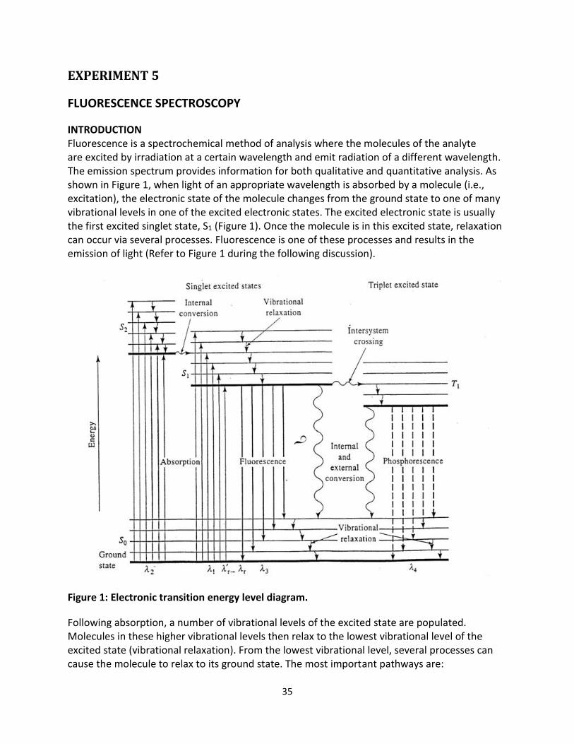
INTRODUCTION Fluorescence is a spectrochemical method of analysis where the molecules of the analyte are excited by irradiation at a certain wavelength and emit radiation of a different wavelength. The emission spectrum provides information for both qualitative and quantitative analysis. As shown in Figure 1, when light of an appropriate wavelength is absorbed by a molecule (i.e., excitation), the electronic state of the molecule changes from the ground state to one of many vibrational levels in one of the excited electronic states. The excited electronic state is usually the first excited singlet state, S1 (Figure 1). Once the molecule is in this excited state, relaxation can occur via several processes. Fluorescence is one of these processes and results in the emission of light (Refer to Figure 1 during the following discussion).

Figure 1: Electronic transition energy level diagram.

Following absorption, a number of vibrational levels of the excited state are populated. Molecules in these higher vibrational levels then relax to the lowest vibrational level of the excited state (vibrational relaxation). From the lowest vibrational level, several processes can cause the molecule to relax to its ground state. The most important pathways are:

36

1. Collisional deactivation (external conversion) leading to nonradiative relaxation.

2. Intersystem Crossing (10-9

s): In this process, if the energy states of the singlet state overlaps those of the triplet state, as illustrated in Figure 1, vibrational coupling can occur between the two states. Molecules in the single excited state can cross over to the triplet excited state.

3. Phosphorescence: This is the relaxation of the molecule from the triplet excited state to the

singlet ground state with emission of light. Because this is a classically forbidden transition, the triplet state has a long lifetime and the rate of phosphorescence is slow

(10-2

to 100 sec). 4. Fluorescence: Corresponds to the relaxation of the molecule from the singlet excited state

to the singlet ground state with emission of light. Fluorescence has short lifetime (~10-8

sec) so that in many molecules it can compete favorably with collisional deactivation, intersystem crossing and phosphorescence. The wavelength (and thus the energy) of the light emitted is dependent on the energy gap between the ground state and the singlet excited state. An overall energy balance for the fluorescence process could be written as:

where Efluor

is the energy of the emitted light, Eabs

is the energy of the light absorbed by the

molecule during excitation, and Evib

is the energy lost by the molecule from vibrational

relaxation. The Esolv.relax

term arises from the need for the solvent cage of the molecule to

reorient itself in the excited state and then again when the molecule relaxes to the ground state. As can be seen from Equation (1), fluorescence energy is always less than the absorption energy for a given molecule. Thus the emitted light is observed at longer wavelengths than the excitation.

5. Internal Conversion: Direct vibrational coupling between the ground and excited electronic states (vibronic level overlap) and quantum mechanical tunneling (no direct vibronic overlap but small energy gap) are internal conversion processes. This is a rapid process

(10-12

sec) relative to the average lifetime of the lowest excited singlet state (10-8

sec) and therefore competes effectively with fluorescence in most molecules.

Other processes, which may compete with fluorescence, are excited state isomerization, photoionization, photodissociation and acid-base equilibria. Fluorescence intensity may also be reduced or eliminated if the luminescing molecule forms ground or excited state complexes (quenching). The quantum yield or quantum efficiency for fluorescence is therefore the ration of the number of molecules that luminesce to the total number of excited molecules. According

37

to the previous discussion, the quantum yield (φ) for a compound is determined by the

relative rate constants (kx) for the processes which deactivate the lowest excited singlet states, namely, fluorescence (kf), intersystem crossing (ki), external conversion (kec), internal conversion (kic), predissociation (kpd), and dissociation (kd).

B. EXPERIMENT SUMMARY In this experiment:

1. the excitation and emission spectra for the fluorescent dye fluorescein will be measured. 2. the effect of concentration and instrumental bandwidth on the fluorescent signal will be

studied. 3. quinine in tonic water will be determined fluorimetrically using a calibration curve and

standard addition.

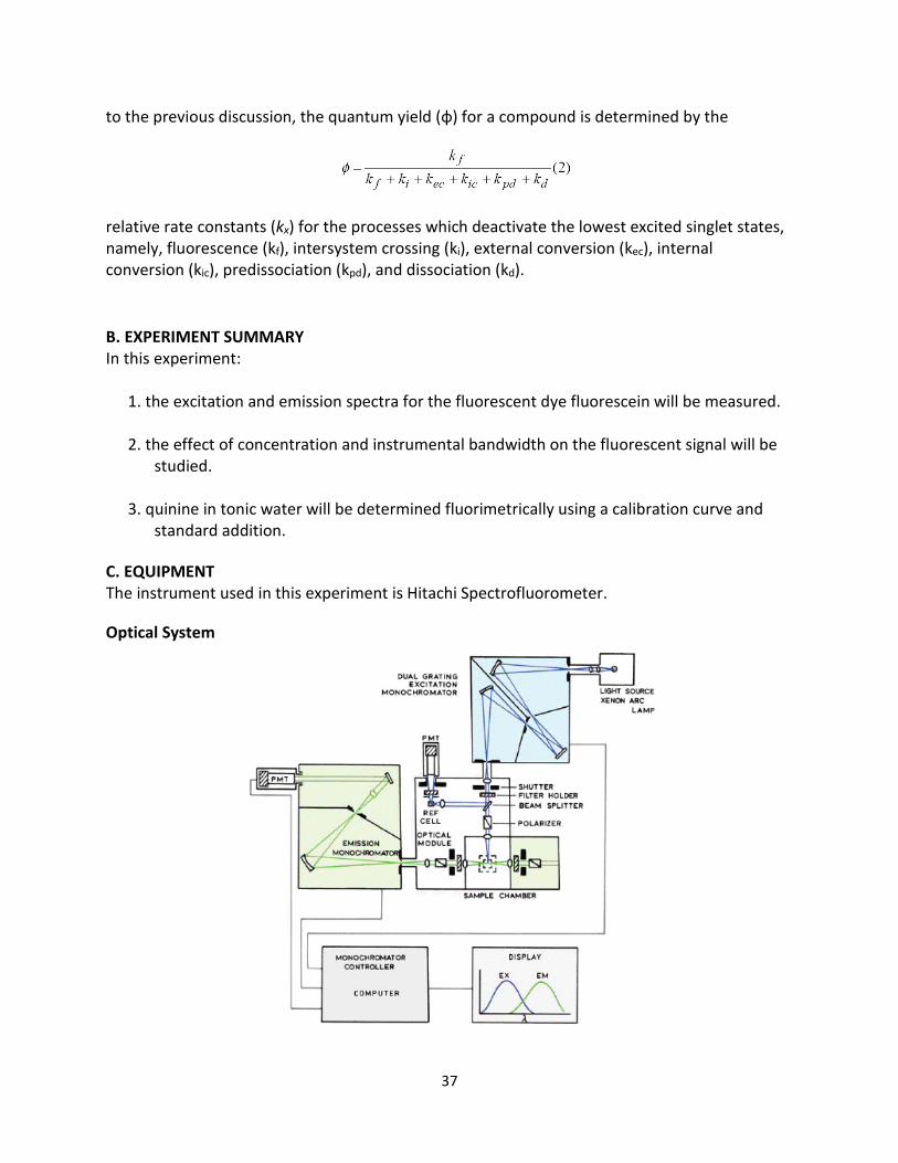
C. EQUIPMENT The instrument used in this experiment is Hitachi Spectrofluorometer.

Optical System

38

A 150 W xenon lamp is used as the light source. The bright spot of the xenon lamp after being

collimated into a beam, is focused via a concave mirror onto the excitation slit assembly

through the entrance slit . Part of the beam, which is then dispersed to a spectrum via the

diffraction grating assembly, is directed out of the exit slit , passes through a collecting lens

assembly, and impinges on the sample cell. For light source compensation, a portion of the

excitation light is reflected by a beam splitter quartz plate to a Teflon reflecting plate. The

scattered light from Teflon plate is directed to a monitor photomultiplier. The emitted light

from the cell is passed through a lens, and directed into the emission monochromator,

consisting of the slit assembly and a diffraction grating assembly. The spectral light is reflected

from a convex mirror and directed to the measurement photomultiplier.

D. EXPERIMENTAL D.1. Start-Up See the instructor to learn how to start up the instrument. Prepare solutions while the instrument is warming up. D.2. Solutions i. Tonic water solutions 1. Solution TW10: Dilute the tonic water by a factor of 10 in 0.1 M H

2SO

4 . Pipette 10.0 mL of tonic water into a

clean 100 mL volumetric flask and fill to the mark with 0.1 M H2SO

4.

2. Solution TW 200: Pipette 5.0 mL TW10 into a clean 100 mL volumetric flask and filling to the mark with 0.1 M H

2SO

4 . Calculate how many times the original tonic water has been diluted.

ii. Solutions for Standard Addition Method Pipette 5 mL of TW10 solution into each of five 100 mL volumetric Flasks. Dilute the first volumetric flask to volume with 0.1 M H

2SO

4 . Then pipette 1 mL of the stock 10 ppm quinine

solution to the second volumetric flask and dilute with 0.1 M H2SO

4. Repeat by pipetting 2, 3,

and 5 mL to the third, fourth and fifth volumetric flask respectively and again dilute each to volume with 0.1 M H

2SO

4 . Calculate how many times the original tonic water has been diluted.

iii. Fluorescein solution (1000 ppm in 95 % ethanol) D.3. Excitation and Emission Spectra of Fluorescein Fluorescence spectroscopy can yield low detection limits, high sensitivity and high

specificity. The high specificity is largely due to the fact that fluorophores exhibit specific

excitation (absorption) and emission (fluorescence) wavelengths. These wavelengths can be

determined via the collection of two spectra, an excitation spectrum and an emission spectrum.

Although the approximate excitation and emission wavelengths for many molecules are known,

these wavelengths should generally be optimized for the specific conditions employed.

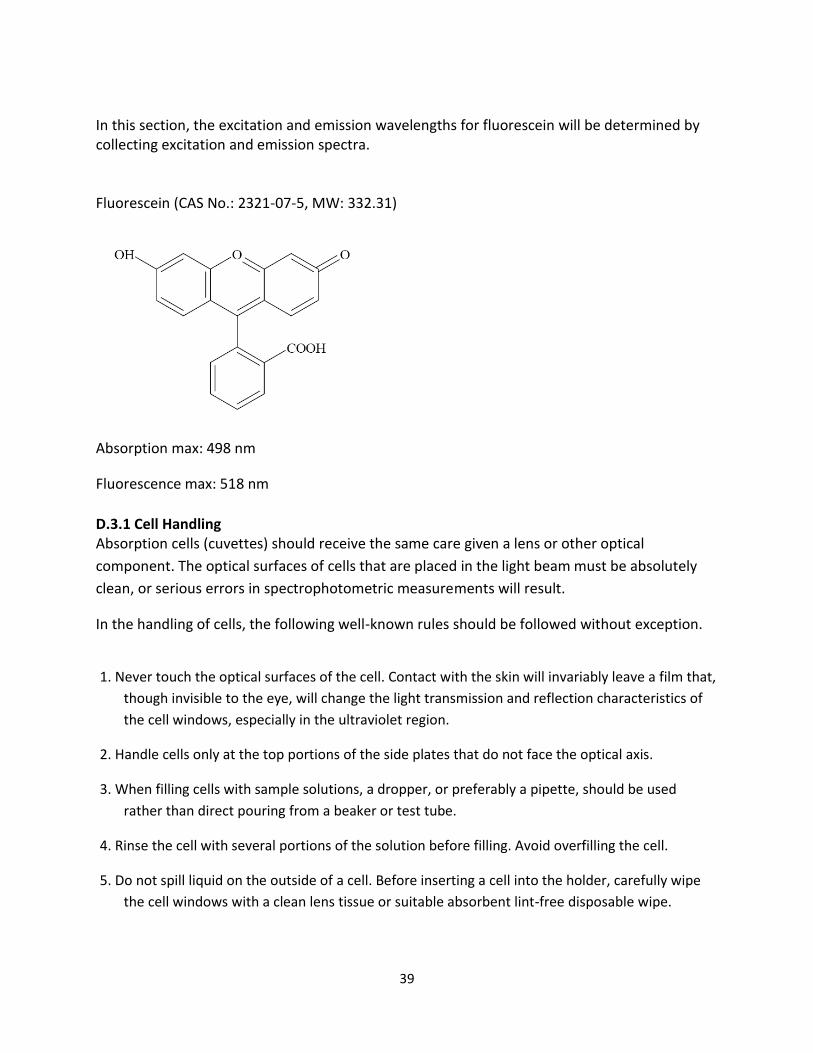
39

In this section, the excitation and emission wavelengths for fluorescein will be determined by collecting excitation and emission spectra. Fluorescein (CAS No.: 2321-07-5, MW: 332.31)

Absorption max: 498 nm

Fluorescence max: 518 nm

D.3.1 Cell Handling Absorption cells (cuvettes) should receive the same care given a lens or other optical

component. The optical surfaces of cells that are placed in the light beam must be absolutely

clean, or serious errors in spectrophotometric measurements will result.

In the handling of cells, the following well-known rules should be followed without exception.

1. Never touch the optical surfaces of the cell. Contact with the skin will invariably leave a film that,

though invisible to the eye, will change the light transmission and reflection characteristics of

the cell windows, especially in the ultraviolet region.

2. Handle cells only at the top portions of the side plates that do not face the optical axis.

3. When filling cells with sample solutions, a dropper, or preferably a pipette, should be used

rather than direct pouring from a beaker or test tube.

4. Rinse the cell with several portions of the solution before filling. Avoid overfilling the cell.

5. Do not spill liquid on the outside of a cell. Before inserting a cell into the holder, carefully wipe

the cell windows with a clean lens tissue or suitable absorbent lint-free disposable wipe.

40

6. Always orient cells in the same direction in the cell holder. When using a matched pair of cells,

always use the same cell for the reference.

7. For the disposable plastic cells, solvents like methanol and ethanol can be contained for a

maximum time of 5 min. Never use the plastic cells for toluene.

D.3.2 Emission Spectrum Note: For the fluorescein analysis, the plastic disposable cuvettes are used.

Find fluorescein’s approximate absorption maximum (498 nm).

With the excitation wavelength fixed at 498 nm, obtain the emission spectrum between 350 and

670 nm.

Scanning Speed: medium

Slit Width: Ex = 3.5 and Em = 3.5

You may need to adjust these.

Fill a plastic cuvette with the solution of 10-ppm fluorescein in 95% ethanol. Fill the cuvette with a

disposable pipette. Place the cuvette into the sample compartment, and close the cover of the

spectrofluorometer.

Ask your instructor how to obtain an emission spectrum.

Locate the exact wavelength of the maximum.

D.3.3 Excitation Spectrum Repeat the same procedure as for the emission spectrum, ensuring that the following parameters

have been adjusted.

Em Wavelength: the value you have just obtained.

Ex Wavelength: 350 - 670 nm

Once the parameters are correctly set, run the spectrum. Locate the excitation maximum. D.4. Inner Filter Effect

In this experiment, you will monitor the fluorescence intensity of Fluorescein as a function of concentration. Prepare the following solutions: 0.1, 1.0, 10 and 100 from the stock 1000 ppm Fluorescein in 95% ethanol. You will measure the relative fluorescence intensity over a set period of time.

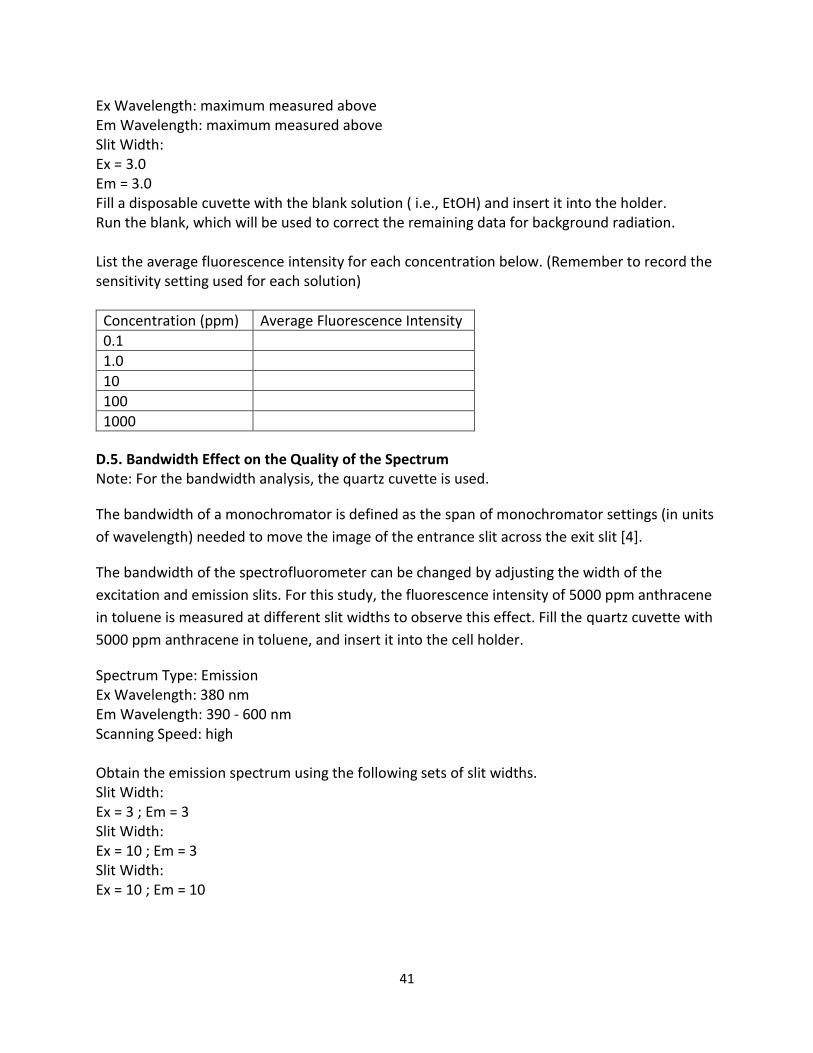
41

Ex Wavelength: maximum measured above Em Wavelength: maximum measured above Slit Width: Ex = 3.0 Em = 3.0 Fill a disposable cuvette with the blank solution ( i.e., EtOH) and insert it into the holder. Run the blank, which will be used to correct the remaining data for background radiation. List the average fluorescence intensity for each concentration below. (Remember to record the sensitivity setting used for each solution)

Concentration (ppm) Average Fluorescence Intensity

0.1

1.0

10

100

1000

D.5. Bandwidth Effect on the Quality of the Spectrum Note: For the bandwidth analysis, the quartz cuvette is used.

The bandwidth of a monochromator is defined as the span of monochromator settings (in units

of wavelength) needed to move the image of the entrance slit across the exit slit [4].

The bandwidth of the spectrofluorometer can be changed by adjusting the width of the

excitation and emission slits. For this study, the fluorescence intensity of 5000 ppm anthracene

in toluene is measured at different slit widths to observe this effect. Fill the quartz cuvette with

5000 ppm anthracene in toluene, and insert it into the cell holder.

Spectrum Type: Emission Ex Wavelength: 380 nm Em Wavelength: 390 - 600 nm Scanning Speed: high Obtain the emission spectrum using the following sets of slit widths. Slit Width: Ex = 3 ; Em = 3 Slit Width: Ex = 10 ; Em = 3 Slit Width: Ex = 10 ; Em = 10

42

D.6 Analysis of Quinine in Tonic Water- Calibration Curve Method Note: For the quinine analysis, the plastic disposable cuvettes are used. In this section, a calibration curve of quinine will be constructed using a series of standard solutions you will prepare. The concentrations of these solutions are 0.1, 0.2, 0.3, 0.4, 0.5 and 0.6 ppm. The excitation and emission maximums for quinine are 350 and 445 nm respectively. The exact maximums may differ from those given above. You may want to determine what they are exactly under our experimental conditions. Change to the following settings: Ex Wavelength: 350 Em Wavelength: 445 Slit Width: Ex = 3 ; Em = 3 Run a blank solution sample before beginning with the standards. Place the first standard in the cell holder and obtain an intensity measurement. Repeat with the

remaining standards to complete the calibration curve. Then, insert the TW200 example you

prepared into the cell holder and obtain an intensity measurement. List the intensity values in a

table.

D.7. Analysis of Quinine in Tonic Water – Standard Addition Method Another method of quantification, standard addition, involves adding varying quantities of a standard to a constant concentration of unknown. These are the solutions that you prepared at the beginning of the lab. Adjust the parameters as follows: Ex Wavelength: 350 Em Wavelength: 445 Slit Width: Ex 3 ; Em 3 Insert a blank solution in the sample holder and run the blank to correct for the background. Measure the intensities of all five solutions that you have made using the same procedure described in section D.4. List the intensity values in a table.

E. DATA PROCESSING AND QUESTIONS

1. Considering its molecular structure, why would you expect fluorescein to be highly fluorescent?

2. What causes the inner filter effect for fluorescein? How can errors due to this effect be

reduced or eliminated? 3. What effects on the spectrum do the excitation and emission bandwidth have? Why?

43

4. From the values obtained in the calibration curve analysis, determine the concentration (in ppm) of quinine in the tonic water.

5. Starting with F=Kc (where, F is fluorescence intensity; K is a constant which depends on the

quantum efficiency of the fluorescent process; and c is concentration: derive an expression relating fluorescence intensity to concentrations and volumes in the standard addition method.

6. Using the expression you derived, plot a linear curve with your standard addition data. Using

the slope and intercept of the plot (and any other known values that you might need) calculate the concentration of quinine in the tonic water. Do not determine the concentration graphically!

7. Do the results from the calibration curve agree with those by standard addition? If so what

does this prove? If not, what does this prove, and which do you think is correct? 8. When would standard addition be more suitable than a calibration curve for quantitative

analysis? 9. In this experiment, you optimized literature excitation and emission wavelength maxima

prior to actual analysis. How would you go about determining and optimizing excitation and emission wavelength maxima for an analyte without any literature data?

F. REFERENCES 1. J. E. O'Reilly, J. Chem. Ed. 1975, 52, 610. 2. Skoog, Holler and Crouch. Chapter 15. 3. R. D. Baun, Introduction to Instrumental Analysis, McGraw-Hill, NY, 1987, Chapter 11. 4. Skoog, Holler and Crouch. Chapter 7.

44

Experiment 7.

Qualitative Gas Chromatography: The Van Deemter plot and optimum

separation

Prelab preparations

Check the chemical structures and boiling points of benzene, toluene, ethyl benzene, and xylenes Obtain

the formulae to calculate N, H, and k’ of an eluted species. Review Van Deemter equation and the

method of internal standard.

Overview BTEX is a commonly used abbreviation for the compounds benzene, toluene, ethyl benzene,

and xylenes. BTEX is used as an octane booster as it has an octane number greater than 100. BTEX is the

component which is responsible for the majority of the toxicity of unleaded gasoline. Moreover, the

relatively high water solubility of the BTEX components relative to the aliphatics in gasoline leads to

contamination of ground waters whenever there is a gasoline spill.

This experiment is comprised of 3 sections as follows: 1) To study the effect of column gas flow rate on

the isothermal separation of the BTEX mixture. 2) To study the effect of column temperature on the

separation of a BTEX mixture. 3) To perform quantitative measurement of BTEX components in a 94-

octane gasoline by the method of internal standard.

Materials

Students are provided with the following standards. (a) Individual standard solution of benzene,

toluene, ethylbenzene and xylenes in hexane at a concentration of 1000 ppm. Each contains 1,000 ppm

bromobenzene. (b) 4 calibration standards of a mixture of benzene, toluene, ethylbenzene and xylenes

(BTEX) in hexane at a level of 100, 500, 1000 and 2000 ppm (µL/L ). The total concentration of xylenes,

consisting of a mixture of three isomers, is a factor of three times higher. There are three structural

isomers in the xylene sample, two of which cannot be resolved from one another. Each standard

mixture also contains 1,000 ppm bromobenzene as the internal standard. (c) A 94-octane gasoline

45

sample is prepared in 10,000 ppm by volume in hexane. This sample also contains bromobenzene as the

internal standard at 1,000 ppm.

Hexane is very volatile. Keep all solution vials tightly closed when not in use.

References: Review chapters 26 & 27 of Skoog/Holler/Nieman, Principles of Instrumental Anlaysis, (5th

edition, 1998, Saunders College Publishing, Florida) for theory of chromatography and GC. Review

Chapter 5 of Harris, Qualitative Chemical Analysis, (5th Ed., Freeman, 1999) for the internal standard

procedure.

The journal article titled Injection Techniques in Capillary GC, Anal. Chem., 1994, 66(20), 1009A-1019A

contains examples of significant errors that can arise at the sample injection step.

Additional information can be found in Gas Chromatography, A Practical Approach, P. J. Baugh, ed.,

1993, Oxford University Press. This book covers the quantitative principles of chromatography quite

well.

PROCEDURE

(1) Effect of column gas flow rate on isothermal GC separation of BTEX compounds (Van Deemter

equation)

Run a sample of hexanes. Select an oven temperature of 55 °C and linear gas velocity of 30 cm/s for the

run.

Meanwhile, prepare and run a 1,000 ppm standard of benzene, a 1,000 ppm standard of toluene, a

1,000 ppm standard of ethyl benzene, and a 1,000 ppm standard of the xylene isomers. Also run a

sample of bromobenzene, because this compound is used as the internal standard later in this

experiment. Run a 1000 ppm BTEX mixture.

46

Q: In this experiment, how do you identify which chromtographic peak corresponds to which

compound? Suggest one method that is more reliable than this? Q: Based on the chemical structures

and boiling points of these four analytes, and knowing the general structure of the stationary phase,

explain the elution order of these compounds.

Now, run the sample (1,000 ppm BTEX standard) isothermally at 55 °C at carrier gas linear velocities of

15, 20, 25, 40 and 50 cm/s.

Q: Calculate number of plates k’, N and H for one compound (e.g. the component with the median k’)

for all runs. Q: Perform the Van Deemter plot and find out the optimal values of H and v. Q: Comment

on the separation of compounds, particularly the (o, p, and m-) xylene isomers.

(2) Effect of column temperature and temperature programming

Set the carrier gas linear velocity to the value calculated in (1).

(a) Effect of column temperature on the isothermal GC separation of BTEX mixture.

Run a 1,000 ppm BTEX standard mixture isothermally at 35, 55 and 75 °C at the optimal carrier gas linear

velocity, or 30 cm/s.

Q: Evaluate the effect of column temperature on separation, resolution, and analysis time in the light of

Rs and k’ values. What compounds should you selected for this evaluation? Q: Does the elution order

change at different temperatures? Confirm the identities of uncertain peaks, if any, by injecting

individual standards.

(b) Effect of column temperature programming on the GC separation of the BTEX mixture

47

Run the 1,000 ppm BTEX standard at the optimal carrier gas initial linear velocity or 30 cm/s using a

linear temperature ramp from 35 °C to 75 °C at 20 °C per minute at constant flow.

Q: Discuss the effect of column temperature programming on separation, resolution and analysis time in

the light of Rs and k’ values. .

(3) Quantitative analysis of BTEX-components in a gasoline sample

Run the gasoline sample `that has already been spiked with the internal standard bromobenzene at

1,000 ppm. Establish a four level calibration (100 to 2,000 ppm) of BTEX standards for the following GC

conditions: carrier gas initial linear velocity of 30 cm/s , and temperature program from 35 °C to 75 °C at

constant flow.

Q: Calculate the peak area ratios for all individual components in BTEX using the method of internal

standards. Q: Perform linear regression analysis and determine the amount of each BTEX component in

the gasoline sample. Estimate the uncertainty associated with your determination. Estimate the

detection limit of your calibration.

48

Experiment 8.

"Imposter" vs. "Real" Perfumes via GC-MS

from J. Chem.Ed, vol. 81, pg. 87-89, 2004. INTRODUCTION The goal of this experiment is to identify "active" ingredients in different fragrances. We would also like to compare name brand fragrances to their imitation counterparts and see if both fragrances really contain the same active ingredients. There are essentially 3 concepts involved in this laboratory exercise besides the underlying fundamentals of gas chromatography (GC). They are: headspace analysis, temperature programming, and mass spectral detection for the purpose of analyte identification. In GC, a sample is typically injected into the inlet with a syringe. Usually the sample injected is a liquid, which is quickly vaporized in the hot inlet. Gaseous samples may also be injected. In the food, flavor, and cosmetics industries smells are very important. This is one example of the utility of headspace analysis. In headspace analysis, the vapor above a sample is drawn into a syringe and injected into the GC. The rationale for this type of sampling is that the molecules responsible for scent are those present in the vapor phase above the sample. If you smell a cup of coffee, the molecules that reach your nose are the volatile ones. We will use this technique to investigate the components responsible for the scent of real and imposter perfumes. In gas chromatography (GC), components of a mixture are separated on the basis of their interaction with a stationary phase within the gas chromatography column. In this experiment, the sample is first injected into a sample inlet, volatilized, and then swept by a carrier gas through the column into a detector. The column is actually a narrow glass capillary in which the walls are coated with a nonpolar liquid film. Components of a mixture are therefore separated based on polarity as well as volatility, with more polar, volatile compounds eluting from the column more quickly than less polar, less volatile compounds. As you might imagine, temperature dramatically influences the degree to which components of the mixture interact with the stationary phase. By changing the temperature of the oven in which the column resides, we have some control over the separation process and can manipulate it to achieve more rapid or more effective separations. Temperature programming is accomplished by ramping the temperature of the column during a separation. The advent of computer-controlled instrumentation has made temperature programming routine. When a mass spectrometer (MS) is used as the detector, eluate from the GC column is immediately swept into an ion source in which the sample is ionized and the abundance of each ion is measured as a function of mass to charge ratio (m/z). Since the charge of most ions formed is +1, the m/z is often referred to simply as the atomic mass of the ion generated. Electron impact ionization is a very “hard” ionization technique, meaning that it involves sufficient energy to not only ionize a molecule, but also fragment the molecule into many smaller pieces. The pattern by which a molecule fragments is characteristic of the structure and functional groups of the molecule. For example, molecules containing an ethyl group often lose

49

the CH2CH3 when ionized. Fragmentation patterns are therefore very useful for qualitatively determining the structure of the original parent molecule! Once the positively charged ions are formed, they are accelerated into a mass analyzer, which separates ions of different masses. There are two methods of obtaining data using GC-MS. The first method is to scan a specified range of m/z ratios. The data can then be plotted as the total ion abundance verses time. This plot, called a Total Ion Chromatogram (TIC) looks like a “regular” chromatogram with peaks at various retention times. Each peak is the sum of the abundance of all ions (regardless of mass) as a function of time. One can also analyze the same data to determine the masses of the fragments that are eluting from the GC column at a specific point in time. In this case, abundance is still plotted on the y-axis, but m/z is plotted on the x-axis to generate a mass spectrum. The fragmentation pattern contained in the mass spectrum is indicative of the compound, and ideally enables one to qualitatively identify each compound as it elutes from the GC. A second method of acquiring data on the GC-MS is called Selective Ion Monitoring, or SIM. In SIM mode, one would select a few m/z ratios that are unique to the compound of interest. The mass filter is then set to detect those select fragments with specific m/z ratios, ignoring all others. This mode minimizes the chance that co elution of an interferent will compromise the detection of a primary species of interest. It also provides maximum sensitivity because the detector spends more time looking for those particular m/z fragments. SIM mode is both more sensitive and selective, but the ability to identify analytes based on mass spectral libraries is sacrificed because an entire mass spectrum is not collected. EXPERIMENTAL METHODS Hazards note: Some perfumes may be irritating and even toxic to people with severe allergies. It is recommended that liquid perfumes be dispensed into septum vials in a fume hood using gloves. Keep perfumes away from extreme heat and open flames. If your instructor has not already done so, tune the mass spectral detector. Obtain 2 small septum vials. In one vial place approximately 0.5 mL of a perfume sample. In the second vial, place approximately 0.5 mL of the corresponding imposter perfume. As you dispense the real and imposter perfumes, smell them, describe the scents and identify any olfactory differences. Select the appropriate stored method file to control the GC-MS instrument. Check each parameter to become familiar with the operating software and be sure your fellow comrades didn’t change it! Injector: we will be making manual injections. Inlet: temperature 250 °C; split mode; split ratio 50:1 Mobile Phase Flow Rate: 1.0 mL/min Oven (controls column temp): 140 °C hold for 20 min Auxiliary (transfer line from GC to MS): temperature 280 °C MS detector: 3.00 minute solvent delay Scan mode from 20 to 500 m/z

50

Step by Step Instructions for Data Collection and Evaluation

1. Once you’ve become familiar with the software and confirmed your operating conditions, prepare to inject 1 μL of a liquid perfume sample. Let the instructor show you how to inject the first time. Collect a Total Ion Chromatogram (TIC) of the sample. Make note of the directory in which you save this and all subsequent chromatograms. 2. After you have collected the first TIC, modify the operating parameters to include a temperature ramp during the run according to the following: a. Initial Temp. 60 oC b. Hold it at 60 oC for 2 minutes c. Ramp at 20 oC/min up to 250 oC d. Hold at 250 oC for 3 minutes. 3. Inject the identical sample as in step 1 - 1 μL of liquid perfume sample. 4. Clean the syringe with methanol or ethanol. 5. Inject 1 μL of the imposter perfume under identical conditions. 6. While chromatograms are being acquired, you may begin analyzing chromatograms already collected. Be sure to make the following part of your analysis: a. Compare the isocratic (fixed temp) and temperature programmed chromatograms. b. Zoom in on the chromatograms to investigate small time windows with multiple peaks. c. Display mass spectra for several peaks. d. Remember each molecule results in a unique fragmentation pattern. Therefore, the pattern from the mass spectrum can be used to identify the molecule. You can compare your mass spectra with those in a mass spectral library. The probability that your mass spectrum matches one in the library should be noted. A probability greater than 90 indicates that there is a high probability that the two compounds are the same, while probabilities less than 50 indicate that substantial differences exist between the unknown and reference mass spectra. e. While looking at the mass spectrum for one of the peaks in a congested area of the total ion chromatogram, make note of the m/z of two or three of the most abundant fragments. You will use these to perform selected ion monitoring (SIM) later in this experiment. f. Using the mass spectral library search feature identify 5 of the components of the perfume sample. Only trust matches that have a probability of 90 or better. Report what scent the volatile "active ingredient” of your fragrance provides. Does it provide a floral, woody or spicy "note?" This will require a little literature searching. Several great articles about this have appeared in Journal of Chemical Education, Analytical Chemistry and Chemical and Engineering News recently. The Sigma Aldrich Catalog of Fragrances and Flavors is an excellent resource for this type of information; as is the internet, particularly a site by the Good Scents Company! g. View the perfume and imposter on the same set of axes in order to better determine compositional differences between the two samples. 7. Set the MS detector to operate in SIM mode at the m/z chosen in step 6e. All other

51

conditions should remain identical. a. As before, inject 1 uL of the genuine perfume. b. When this SIM chromatogram is complete, return the MS to operate according to the original SCAN settings. c. Compare the SIM and TIC chromatograms. 8. Before doing headspace analysis of the perfume, obtain a 50 or 100-μL gas-tight syringe. Change the inlet mode to: a. Pulsed Splitless b. Inj. Pulse Pressure: 30 psi c. Pulse time: 1.0 min. d. Purge Flow: 50 mL/min. e. Purge Time: 0.9 min. i. Note: If your instrument does not have automated pulsed splitless capability, you may want to warm both the samples and the gas-tight syringe in a 40 oC oven to increase headspace concentrations of perfume components. 9. Perform headspace sampling by inserting the syringe into the septum, but not under the surface of the liquid. Draw 50 μL of the VAPOR above the liquid surface into the syringe. Inject the gas sample into the GC. Collect a TIC. a. View the headspace chromatogram and the liquid chromatogram on the same plot. Based on a comparison of these chromatograms, what can be said about the volatility of most of the components of this mixture? 10. Collect a headspace TIC of the imposter to the perfume you have selected. a. Overlay the real and imposter headspace chromatograms. Identify (using the mass spec library) as many components as you can that are present in the real perfume but missing from the imposter, or vice versa. Why do you think these are missing? OR Why do you think these are present? 11. Clean both syringes with methanol or ethanol. Guide for the Lab Report Submit a Title and Abstract. Focus on the benefits of using a mass spectral detector in the theory section. You should include separate model numbers for the GC and the MSD (mass spectral detector). The procedure should focus primarily on how you obtained the headspace sample. Data to present: TIC of perfume – isocratic TIC of perfume – T programmed TIC of imposter – T programmed (these could be overlaid) SIM chromatogram (identify the major peak) Table of Retention Times, Peak Identities, Characteristic Odors (if found) TICs of real and imposter headspace samples (can be overlaid).

52

Identity of extra or missing components in imposter perfume. Results and Discussion How might extra components contribute to the scent? How would the missing components affect the scent? Does your analytical evaluation support your olfactory observations? Compare the SIM and TIC chromatograms. Consider the y-axes on these chromatograms. Which provides a larger signal for the analyte on which you focused for the SIM? Why does SIM mode offer greater sensitivity?

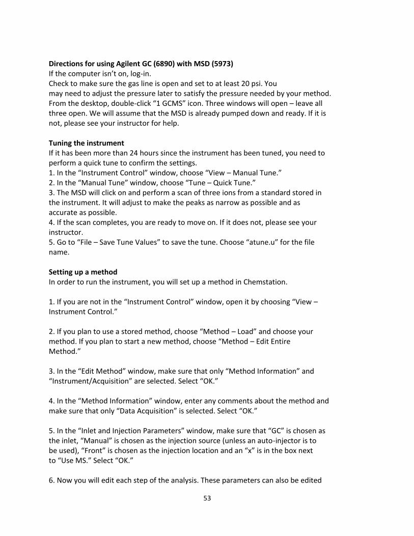
53

Directions for using Agilent GC (6890) with MSD (5973) If the computer isn’t on, log-in. Check to make sure the gas line is open and set to at least 20 psi. You may need to adjust the pressure later to satisfy the pressure needed by your method. From the desktop, double-click “1 GCMS” icon. Three windows will open – leave all three open. We will assume that the MSD is already pumped down and ready. If it is not, please see your instructor for help. Tuning the instrument If it has been more than 24 hours since the instrument has been tuned, you need to perform a quick tune to confirm the settings. 1. In the “Instrument Control” window, choose “View – Manual Tune.” 2. In the “Manual Tune” window, choose “Tune – Quick Tune.” 3. The MSD will click on and perform a scan of three ions from a standard stored in the instrument. It will adjust to make the peaks as narrow as possible and as accurate as possible. 4. If the scan completes, you are ready to move on. If it does not, please see your instructor. 5. Go to “File – Save Tune Values” to save the tune. Choose “atune.u” for the file name. Setting up a method In order to run the instrument, you will set up a method in Chemstation. 1. If you are not in the “Instrument Control” window, open it by choosing “View – Instrument Control.” 2. If you plan to use a stored method, choose “Method – Load” and choose your method. If you plan to start a new method, choose “Method – Edit Entire Method.” 3. In the “Edit Method” window, make sure that only “Method Information” and “Instrument/Acquisition” are selected. Select “OK.” 4. In the “Method Information” window, enter any comments about the method and make sure that only “Data Acquisition” is selected. Select “OK.” 5. In the “Inlet and Injection Parameters” window, make sure that “GC” is chosen as the inlet, “Manual” is chosen as the injection source (unless an auto-injector is to be used), “Front” is chosen as the injection location and an “x” is in the box next to “Use MS.” Select “OK.” 6. Now you will edit each step of the analysis. These parameters can also be edited

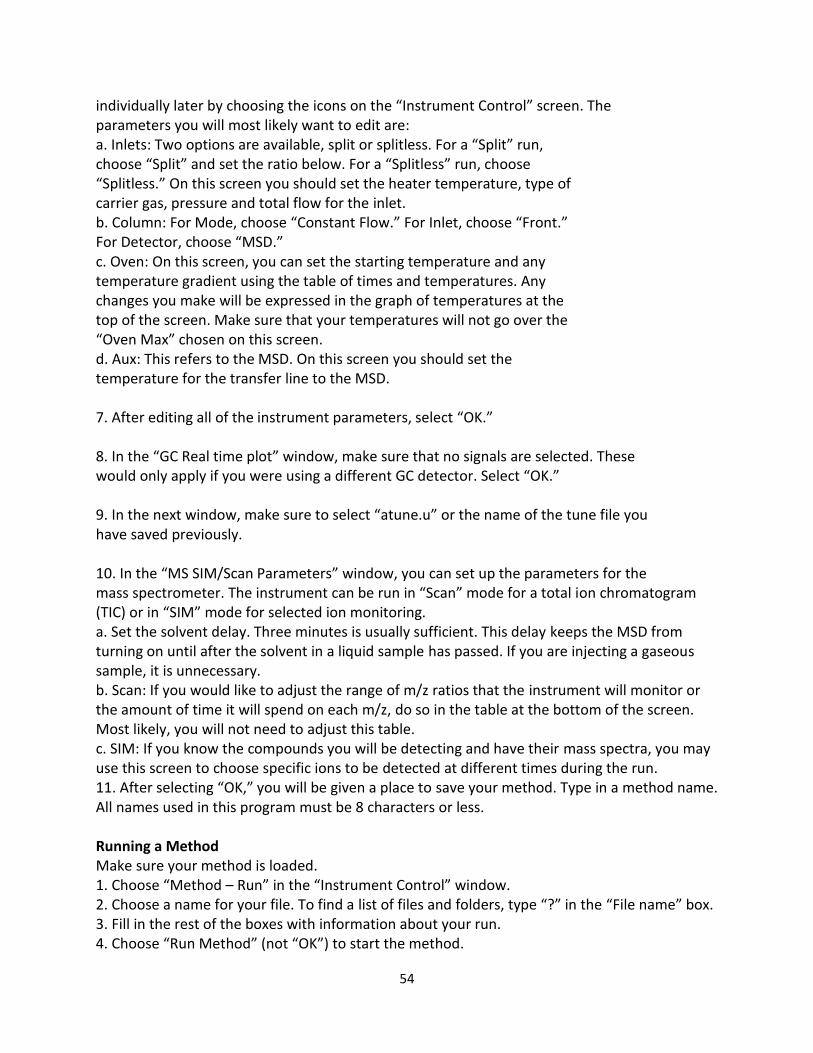
54

individually later by choosing the icons on the “Instrument Control” screen. The parameters you will most likely want to edit are: a. Inlets: Two options are available, split or splitless. For a “Split” run, choose “Split” and set the ratio below. For a “Splitless” run, choose “Splitless.” On this screen you should set the heater temperature, type of carrier gas, pressure and total flow for the inlet. b. Column: For Mode, choose “Constant Flow.” For Inlet, choose “Front.” For Detector, choose “MSD.” c. Oven: On this screen, you can set the starting temperature and any temperature gradient using the table of times and temperatures. Any changes you make will be expressed in the graph of temperatures at the top of the screen. Make sure that your temperatures will not go over the “Oven Max” chosen on this screen. d. Aux: This refers to the MSD. On this screen you should set the temperature for the transfer line to the MSD. 7. After editing all of the instrument parameters, select “OK.” 8. In the “GC Real time plot” window, make sure that no signals are selected. These would only apply if you were using a different GC detector. Select “OK.” 9. In the next window, make sure to select “atune.u” or the name of the tune file you have saved previously. 10. In the “MS SIM/Scan Parameters” window, you can set up the parameters for the mass spectrometer. The instrument can be run in “Scan” mode for a total ion chromatogram (TIC) or in “SIM” mode for selected ion monitoring. a. Set the solvent delay. Three minutes is usually sufficient. This delay keeps the MSD from turning on until after the solvent in a liquid sample has passed. If you are injecting a gaseous sample, it is unnecessary. b. Scan: If you would like to adjust the range of m/z ratios that the instrument will monitor or the amount of time it will spend on each m/z, do so in the table at the bottom of the screen. Most likely, you will not need to adjust this table. c. SIM: If you know the compounds you will be detecting and have their mass spectra, you may use this screen to choose specific ions to be detected at different times during the run. 11. After selecting “OK,” you will be given a place to save your method. Type in a method name. All names used in this program must be 8 characters or less. Running a Method Make sure your method is loaded. 1. Choose “Method – Run” in the “Instrument Control” window. 2. Choose a name for your file. To find a list of files and folders, type “?” in the “File name” box. 3. Fill in the rest of the boxes with information about your run. 4. Choose “Run Method” (not “OK”) to start the method.

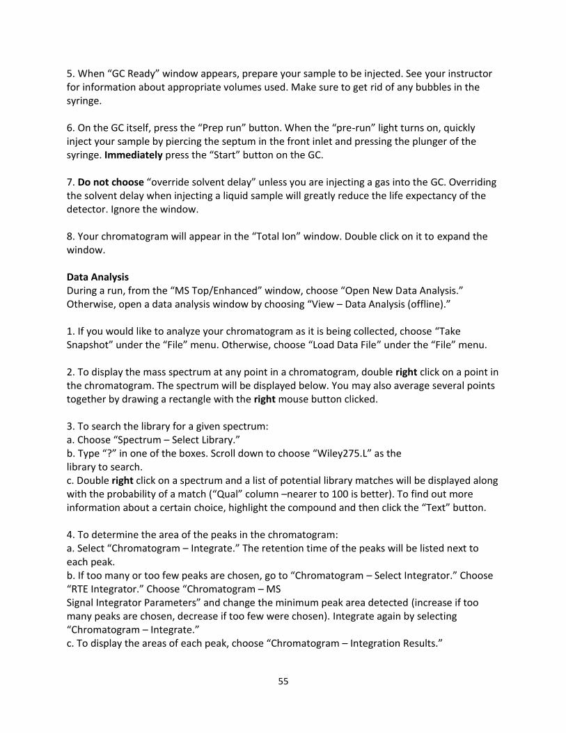
55

5. When “GC Ready” window appears, prepare your sample to be injected. See your instructor for information about appropriate volumes used. Make sure to get rid of any bubbles in the syringe. 6. On the GC itself, press the “Prep run” button. When the “pre-run” light turns on, quickly inject your sample by piercing the septum in the front inlet and pressing the plunger of the syringe. Immediately press the “Start” button on the GC. 7. Do not choose “override solvent delay” unless you are injecting a gas into the GC. Overriding the solvent delay when injecting a liquid sample will greatly reduce the life expectancy of the detector. Ignore the window. 8. Your chromatogram will appear in the “Total Ion” window. Double click on it to expand the window. Data Analysis During a run, from the “MS Top/Enhanced” window, choose “Open New Data Analysis.” Otherwise, open a data analysis window by choosing “View – Data Analysis (offline).” 1. If you would like to analyze your chromatogram as it is being collected, choose “Take Snapshot” under the “File” menu. Otherwise, choose “Load Data File” under the “File” menu. 2. To display the mass spectrum at any point in a chromatogram, double right click on a point in the chromatogram. The spectrum will be displayed below. You may also average several points together by drawing a rectangle with the right mouse button clicked. 3. To search the library for a given spectrum: a. Choose “Spectrum – Select Library.” b. Type “?” in one of the boxes. Scroll down to choose “Wiley275.L” as the library to search. c. Double right click on a spectrum and a list of potential library matches will be displayed along with the probability of a match (“Qual” column –nearer to 100 is better). To find out more information about a certain choice, highlight the compound and then click the “Text” button. 4. To determine the area of the peaks in the chromatogram: a. Select “Chromatogram – Integrate.” The retention time of the peaks will be listed next to each peak. b. If too many or too few peaks are chosen, go to “Chromatogram – Select Integrator.” Choose “RTE Integrator.” Choose “Chromatogram – MS Signal Integrator Parameters” and change the minimum peak area detected (increase if too many peaks are chosen, decrease if too few were chosen). Integrate again by selecting “Chromatogram – Integrate.” c. To display the areas of each peak, choose “Chromatogram – Integration Results.”

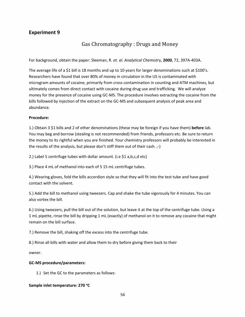
56

Experiment 9

Gas Chromatography : Drugs and Money

For background, obtain the paper: Sleeman, R. et. al. Analytical Chemistry, 2000, 72, 397A-403A.

The average life of a $1 bill is 18 months and up to 10 years for larger denominations such at $100’s.

Researchers have found that over 80% of money in circulation in the US is contaminated with

microgram amounts of cocaine, primarily from cross contamination in counting and ATM machines, but

ultimately comes from direct contact with cocaine during drug use and trafficking. We will analyze

money for the presence of cocaine using GC-MS. The procedure involves extracting the cocaine from the

bills followed by injection of the extract on the GC-MS and subsequent analysis of peak area and

abundance.

Procedure:

1.) Obtain 3 $1 bills and 2 of other denominations (these may be foreign if you have them) before lab.

You may beg and borrow (stealing is not recommended) from friends, professors etc. Be sure to return

the money to its rightful when you are finished. Your chemistry professors will probably be interested in

the results of the analysis, but please don’t stiff them out of their cash. ;-)

2.) Label 5 centrifuge tubes with dollar amount. (i.e $1 a,b,c,d etc)

3.) Place 4 mL of methanol into each of 5 15 mL centrifuge tubes.

4.) Wearing gloves, fold the bills accordion style so that they will fit into the test tube and have good

contact with the solvent.

5.) Add the bill to methanol using tweezers. Cap and shake the tube vigorously for 4 minutes. You can

also vortex the bill.

6.) Using tweezers, pull the bill out of the solution, but leave it at the top of the centrifuge tube. Using a

1 mL pipette, rinse the bill by dripping 1 mL (exactly) of methanol on it to remove any cocaine that might

remain on the bill surface.

7.) Remove the bill, shaking off the excess into the centrifuge tube.

8.) Rinse all bills with water and allow them to dry before giving them back to their

owner.

GC-MS procedure/parameters:

1.) Set the GC to the parameters as follows:

Sample inlet temperature: 270 oC

57

Temperature program: 130 oC for 1 min, ramp at 12 oC/min to 280 oC

He carrier flow: 2 mL/min

Injection type : Splitless

Ion Source Temperature: 230 oC

Injection Volume : 2L

Solvent delay : 8 minutes

2.) Obtain a few milliliters of methanol in a beaker to rinse your syringes.

3 .) Run each of your samples, 2 L injections.

4.) For each spectrum:

a. On the total ion chromatogram (TIC): the peak position of cocaine marked, area of the peak auto

integrated, integrated area of the background of the peak. Consult the instructor for a demonstration on

how to get the background number.

b. On the extracted ion chromatogram (EIC): total abundance of the peak for cocaine in each sample,

total abundance at the same position for a blank.

Data Analysis:

6.) Explain in your report how and why methanol is a good choice for an extraction solvent.

7.) Explain the fragmentation pattern seen in the cocaine EIC.

8.) Was there a correlation between the relative amount of cocaine found and the size of the

denomination?

Note: Extracted ion chromatography is a post-run data manipulation that allows the experimenter to

view the chromatogram as if only one (or a limited set) of ions had been monitored. True single-ion

monitoring is conducted by setting up the mass spectrometer before the analysis so that it collects only

that ion, offering significant improvements in the counts obtained.

58

Experiment 10

59

APPENDIX I

INSTRUMENT OPERATING INSTRUCTIONS

Nicolet Avatar FT-IR

Operating Instructions for the Ocean Optics UV-vis Spectrometer

HP GCD Gas Chromatography Mass Spectrometer

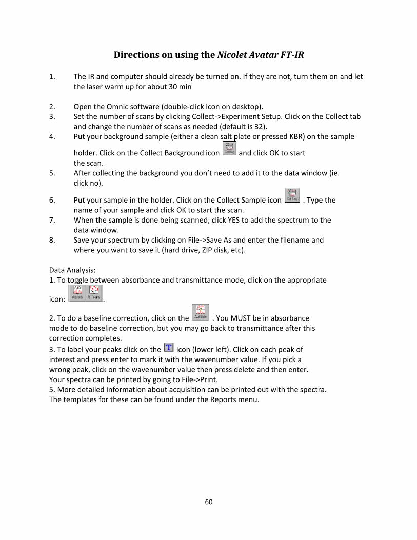
60

Directions on using the Nicolet Avatar FT-IR

1. The IR and computer should already be turned on. If they are not, turn them on and let the laser warm up for about 30 min

2. Open the Omnic software (double-click icon on desktop). 3. Set the number of scans by clicking Collect->Experiment Setup. Click on the Collect tab

and change the number of scans as needed (default is 32). 4. Put your background sample (either a clean salt plate or pressed KBR) on the sample

holder. Click on the Collect Background icon and click OK to start the scan.

5. After collecting the background you don’t need to add it to the data window (ie. click no).

6. Put your sample in the holder. Click on the Collect Sample icon . Type the name of your sample and click OK to start the scan.

7. When the sample is done being scanned, click YES to add the spectrum to the

data window. 8. Save your spectrum by clicking on File->Save As and enter the filename and

where you want to save it (hard drive, ZIP disk, etc). Data Analysis: 1. To toggle between absorbance and transmittance mode, click on the appropriate

icon: .

2. To do a baseline correction, click on the . You MUST be in absorbance mode to do baseline correction, but you may go back to transmittance after this correction completes.

3. To label your peaks click on the icon (lower left). Click on each peak of interest and press enter to mark it with the wavenumber value. If you pick a wrong peak, click on the wavenumber value then press delete and then enter. Your spectra can be printed by going to File->Print. 5. More detailed information about acquisition can be printed out with the spectra. The templates for these can be found under the Reports menu.

61

Operating Instructions for the Ocean Optics UV-vis Spectrometer

Initializing Instrument

1) Make sure USB spectrometer is attached to PC and is plugged into power wall socket. You may need

to restart computer if it is not installed.

2) Double click on OOI icon to start spectrometer program. Make sure that white spectrometer box has

power switch in off (center) position. Make sure you are in scope mode (S is clicked on toolbar).

3) Hit dark current store button (the black light bulb at left side of second toolbar).

4) Turn on lamp (switch white box to on position) and set the spectrometer values [average = 6, boxcar =

10, flash delay = 100 ms]. Adjust integration time so the maximum signal is <4000.

5) Press the yellow light bulb icon to store an initial reference background and then switch the screen to

absorbance mode (A icon on the right side of bottom toolbar).

RECORDING A SPECTRUM

1) Prepare a sample solution that has a visible, but pale color. If your sample is too concentrated the

peaks will be off scale. You do not need to know the absolute concentration of your solution for this

measurement.

2) If computer is on, the spectrometer program is running, and you are in absorbance mode (A is clicked

on the toolbar) and the screen is constantly updating itself. If it is unchanging, click on the camera icon

(static snapshot mode) to bring it back to real time acquisition.

3) Insert a blank (cuvette and solvent) and hit the store reference button (yellow light bulb icon).

4) Replace the blank cuvette with your sample cuvette and the spectrum should immediately appear

and constantly keep updating.

5) Click on the camera icon to get a snapshot and stop the spectrum from updating.

6) Print out your spectrum in landscape mode. Make sure to label it with your sample name!

7) Use the cursor keys to move the green cursor line to your peaks of interest and record the

wavelength on your printout. Use the scale key (button with 4 arrows like compass points) to expand

the spectrum to see if there are any low intensity features.

8) Save your processed spectrum to a file with a descriptive label. The program automatically adds an

extension (.master.absorbance). This file is in ASCII/text format and you can read the data into graphing

programs like Excel or Kalideograph and plot your spectra.

9) Unclick the camera button, remove your sample, and leave the program running for the next user.

62

HP GCD Gas Chromatography Mass Spectrometer Instructions Click on GCD Top to start program

To tune, go to Maintenance, System Verification. Then you want to do a Tune,

But NOT Acquisition and Review Data.

To set a method, go to Method, then Edit.

Do not set any temperatures above 300C!!!

Set parameters.

Injection temperature: Temperature of the injection port.

Initial temperature: Temperature of the oven upon injection.

Initial time: Amount of time that the oven stays at the initial temperature.

(For an isocratic run, you don’t need to set any other temps. Make sure all rates are

zero.)

Rate box: For use with gradient runs. Set a temperature to increase to, a rate of

temperature increase (0-70C/min), and a time to hold that temperature constant in

the oven. All of these go across on one row of the table. You can set more than

one step of the gradient.

Flow rate: The rate of the gas flow through the column. Generally keep it around

0.7 mL/min.

Mass range: The range of mass to charge ratios the mass spectrometer detects.

Save the method.

Go to Inject, then One Sample.

Type in name to save your file as, operator name, name of your sample, etc.

Hit run, then get your sample ready. Rinse syringe w/ sample several times. Pull up

about 1 μL of sample into the syringe followed by ~3 μL of air. When red light on GC

goes off, you can inject. Hold syringe in injection port for ~5 s, then push down

plunger to inject and hit start on the GC. Hold syringe in place for ~15 s, then remove.

Rinse out the syringe several times with solvent.

63

Review Data to see the chromatogram.

To zoom in on a peak, click and drag a box with the left mouse button.

To view the mass spectrum of the peak, double click with the right mouse button at the

center of the peak.

To identify the peak, go to Identify, then Search Spectrum.

64

APPENDIX II USE OF A MICROSYRINGE Liquid samples can conveniently be injected into a gas chromatograph (GC) with a microsyringe. These syringes are calibrated so that a fixed volume of liquid remains in the needle before and after the injection. However, in the GC the sample is usually injected into a heated zone where some of the liquid vaporizes from the needle, thus delivering a larger sample than intended. Following are the manufacturer's suggestions on the use of a microsyringe.

A. Filling Grasping only the syringe flange and plunger, pump out the air, and overfill the syringe. Then, grasping the flange and plunger, hold the syringe perpendicular to one's master eye and against a white background. Bring the syringe plunger just to the top of the scribe line of the desired volume. Lightly blot the needle, being careful not to pull liquid out of the syringe needle. Now back off the plunger, pulling the liquid from the needle into the syringe. The total liquid is now read. Insert the needle through the rubber septum and quickly discharge the volume. Rapidly withdraw the needle. Now withdraw the plunger and read the residual liquid. The difference in the initial and final volume is the liquid injected. B. General Comments

A few pumps with the liquid being transferred will give adequate lubrication. (The use of grease as a lubricant generally results in a split glass barrel.) If the plunger is withdrawn completely from the syringe wipe carefully before replacing. Perspiration and soil from one's fingers will very often cause a sticky plunger or occasionally will even freeze it solid in the glass. In using the syringe as outlined above, we have found it necessary to keep fingers from the syringe barrel. The syringe is filled and handled by the flange and the plunger button. Thus, the heat of the hand does not throw off the measurements, which can cause variations as high as 0.3 μL. By observing the preceding techniques, one can routinely calibrate to the accuracy of the laboratory balance, which is 0.1 milligrams or 0.1 μL when using water.

C. Cleaning

Detergent and water, glacial acetic acid, nitric acid, or common laboratory organic solvents will clean quite well. If a plunger is withdrawn and handled or exposed to dust, carefully wipe it with tissue before replacing it in the syringe. In this course it will be sufficient to flush the syringe with a volatile organic solvent and then dry it by pumping the plunger several times. NOTE: Since there is a positive pressure of helium gas flowing through the gas chromatograph at all times, it is imperative that you keep hold of the syringe plunger, otherwise the plunger is easily forced out of the syringe, negating the results of that particular sample.