Embed Size (px)
Citation preview

The University of Reading
INSTRUMENTATION FOR ATMOSPHERIC ION MEASUREMENTS
Karen Louise Aplin
A thesis submitted for the degree of Doctor of Philosophy
Department of Meteorology
August 2000

Instrumentation for atmospheric ion measurements
2
Abstract Small ions are part of the atmospheric aerosol spectrum, and study of ion-aerosol
interactions is fundamental in atmospheric physics. Air ion physics and
instrumentation are reviewed, including the historical context. A miniaturised Gerdien
condenser for ion measurement, operating in situ to minimise inlet errors, is
described. Two operating modes using independent current and voltage decay
measurements are employed. A more sophisticated self-calibrating and fully
programmable ion mobility spectrometer (PIMS) based on the same principles, is also
discussed. Detailed analysis of error terms and application of new technology is
demonstrated to greatly improve its capability. A variety of self-consistent
experimental approaches, including ionisation and ion concentration instruments, is
used to calibrate the new PIMS instrument.
In developing and characterising the individual components of the PIMS, favourable
and unfavourable operating régimes are identified: this approach can also be applied
to other aspiration ion counting techniques. Use of a sophisticated programmable
electrometer permits compensation for leakage terms. Electrically-charged aerosol
particles have been found to complicate the ion measurements. Consequently,
conventional ion-aerosol theory, which neglects the particulate concentration, is
thought to be incomplete. The polymodal ion mobility spectrum is also found to
influence the instruments operation.
The classical theory for calculating air conductivity from voltage decay measurements
is modified to take account of the ion mobility spectrum, and a new technique to
obtain ion mobility spectra by inversion is presented. Ion mobility spectra are also
derived using conventional ion current measurements, and the two methods of
obtaining ion spectra from independent PIMS measurements are shown to be
consistent. Development of the novel programmable ion instrumentation, in
conjunction with consideration of the ion mobility spectrum yields an improved and
flexible approach to in situ atmospheric ion measurements.

Instrumentation for atmospheric ion measurements
3
Acknowledgements
This project was funded by the Natural Environment Research Council. I would like
to thank Dr. Giles Harrison for his continual guidance and boundless enthusiasm for a
subject that has also captured my imagination. The Meteorology Department technical
team all deserve special thanks: Andrew Lomas for lots more than sorting out my PC
problems and messy cables, and Stephen Gill for his excellent workmanship and
coming to rescue me from Mace Head. Assistance in all matters electronic was
provided by Roger Knight, who also helped to proof-read, and Steven Tames.
I have had extremely interesting and useful conversations with Dr. Charles Clement
throughout the course of my studies. Dr. Jyrgi Mäkelä provided valuable insight
during the long afternoon in Geneva when he was unable to escape my questioning.
My family and friends have been extremely supportive and encouraging, particularly
during difficult times. My mother and brother Mark proof-read the majority of this
Thesis. Marks comments in particular were both helpful and hilarious during the long
days of writing up. I thank Daniel Meacham for his friendship, humour and interest in
my work. My late hamster, Hilary, was always an endearing distraction.
The musical life of the Meteorology Department has added an extra dimension to my
time here. My devotion to one musical instrument has occasionally superseded my
commitment to the scientific instruments I chose to make my career. It, and the people
I meet with similar interests continue to inspire me.

Instrumentation for atmospheric ion measurements
4
Contents Abstract ............................................................................................................................... 2 Acknowledgements ............................................................................................................. 3 Contents............................................................................................................................... 4 Table of Figures .................................................................................................................. 8 Nomenclature .................................................................................................................... 15 1 Ions in the Atmosphere............................................................................................... 17
1.1 Introduction.......................................................................................................... 17 1.2 Atmospheric aerosol ............................................................................................ 18
1.2.1 Aerosol nucleation......................................................................................... 19 1.2.2 The solar cycle and climate........................................................................... 20
1.3 Atmospheric small ions........................................................................................ 20 1.3.1 Production of atmospheric ions..................................................................... 21 1.3.2 Size and composition of atmospheric small ions .......................................... 22 1.3.3 Mobility of atmospheric small ions............................................................... 22 1.3.4 The ion balance equation............................................................................... 23
1.4 Ions in the global atmospheric electrical circuit .................................................. 24 1.5 Measurement of atmospheric small ions.............................................................. 25 1.6 Motivation............................................................................................................ 26 1.7 Thesis Structure ................................................................................................... 27
2 The significance of atmospheric ion measurements................................................... 29 2.1 Historical introduction ......................................................................................... 29 2.2 Overview of the Gerdien method......................................................................... 30
2.2.1 Principles of the Gerdien Condenser............................................................. 30 2.2.2 Calculating conductivity from Gerdien condenser measurements................ 33 2.2.3 Fair weather measurements of conductivity at the ground ........................... 38
2.3 Fair weather measurements at altitude................................................................. 42 2.4 Errors in the Gerdien method............................................................................... 44 2.5 Air conductivity and aerosol pollution ................................................................ 47 2.6 Ion mobility spectrometry with a cylindrical condenser...................................... 50
2.6.1 Theory ........................................................................................................... 51 2.6.2 Instrumentation.............................................................................................. 52 2.6.3 Air ion mobility spectra................................................................................. 56
2.7 Nucleation ............................................................................................................ 59 2.7.1 Nucleation onto ions...................................................................................... 60 2.7.2 Laboratory observations of nucleation.......................................................... 62 2.7.3 Observations of nucleation in the atmosphere .............................................. 66 2.7.4 Models........................................................................................................... 68
2.8 Conclusions.......................................................................................................... 73 3 A miniaturised Gerdien device ................................................................................... 75
3.1 Design criteria ...................................................................................................... 75 3.1.1 Tube material and dimensions....................................................................... 75 3.1.2 Flow rates ...................................................................................................... 80 3.1.3 Measuring the ion signal ............................................................................... 83 3.1.4 Switching devices in electrometry ................................................................ 90
3.2 Characterisation of individual components of the Gerdien system ..................... 92 3.2.1 Flow properties of air in the Gerdien tube .................................................... 92

Instrumentation for atmospheric ion measurements
5
3.2.2 A simplified relationship between critical mobility and maximum radius ... 95 3.2.3 Measurement System .................................................................................... 97
3.3 Implementation of the Gerdien system .............................................................. 102 3.3.1 Measuring physical properties of ions with the Gerdien system ................ 103 3.3.2 Calibration in clean air ................................................................................ 104 3.3.3 Measurements in both Voltage Decay and current modes.......................... 105
3.4 Conclusions........................................................................................................ 108 4 A switched mobility Gerdien ion counter................................................................. 109
4.1 Justification and strategy.................................................................................... 109 4.2 The microcontrolled system............................................................................... 109
4.2.1 Analogue to digital converter ...................................................................... 110 4.2.2 Switching circuitry ...................................................................................... 111 4.2.3 Software ...................................................................................................... 112 4.2.4 Serial communication.................................................................................. 112
4.3 Results with the microcontrolled system ........................................................... 113 4.4 Conclusions........................................................................................................ 114
5 The Programmable Ion Mobility Spectrometer........................................................ 115 5.1 Motivation.......................................................................................................... 116
5.1.1 Limitations of other systems ....................................................................... 116 5.2 Objectives .......................................................................................................... 116
5.2.1 New features of the system ......................................................................... 117 5.2.2 New tube design .......................................................................................... 119
5.3 Programmable bias voltage circuitry ................................................................. 121 5.4 The multimode electrometer .............................................................................. 123
5.4.1 Description .................................................................................................. 123 5.4.2 Calibration of the MME .............................................................................. 127 5.4.3 Voltage follower mode................................................................................ 128
5.5 Calibration of MME Picoammeter Mode .......................................................... 129 5.5.1 Resistive calibration techniques .................................................................. 129 5.5.2 A capacitative calibration technique: the femtoampere current reference .. 132
5.6 Testing of MME measurement modes............................................................... 133 5.6.1 Error term modes......................................................................................... 133 5.6.2 Compensating for leakage currents in the ion current measurement .......... 135 5.6.3 Switching transients .................................................................................... 137 5.6.4 Electrometer control software ..................................................................... 137
5.7 Integrated PIMS system..................................................................................... 138 5.7.1 Measurement of capacitance of Gerdien condenser.................................... 138 5.7.2 Complete control program .......................................................................... 140 5.7.3 Timing and Synchronisation ....................................................................... 142 5.7.4 Testing the integrated PIMS systems .......................................................... 143
5.8 Conclusions........................................................................................................ 145 6 PIMS atmospheric calibration and testing................................................................ 147
6.1 Description of PIMS atmospheric deployment.................................................. 149 6.2 Calibration of raw data....................................................................................... 150
6.2.1 Current Measurement method..................................................................... 150 6.2.2 Voltage Decay method ................................................................................ 153
6.3 Comparisons of PIMS data with ion production rate......................................... 159 6.4 PIMS ion measurement mode intracomparisons ............................................... 162
6.4.1 Likely origin of conductivity offsets ........................................................... 163 6.4.2 Negative conductivities ............................................................................... 165

Instrumentation for atmospheric ion measurements
6
6.4.3 Temporal inconsistencies ............................................................................ 165 6.5 PIMS systems intercomparisons ........................................................................ 166
6.5.1 Local variations between the PIMSs........................................................... 169 6.6 Comparing PIMS data to other ion measurements ............................................ 170
6.6.1 Ion measurements made with another design of Gerdien Condenser ......... 170 6.7 Average conductivities....................................................................................... 173 6.8 Conclusions........................................................................................................ 179
7 Variability in PIMS measurements........................................................................... 180 7.1 Effect of fluctuations in the flow ....................................................................... 180
7.1.1 The contribution of intermediate ions to conductivity ................................ 180 7.1.2 Effect on the fraction of ions measured ...................................................... 183
7.2 Physical differences between the modes............................................................ 186 7.3 Offset currents measured at zero bias voltage ................................................... 187 7.4 Ionic sources of noise......................................................................................... 193
7.4.1 Atmospheric ion fluctuations ...................................................................... 193 7.4.2 Shot noise .................................................................................................... 194
7.5 Conclusions........................................................................................................ 194 8 Observations of ion spectra and ion-aerosol interactions......................................... 196
8.1 Ion spectra .......................................................................................................... 196 8.2 Effect of ion mobility spectrum on voltage decays ........................................... 198
8.2.1 Voltage decay for a parameterised mobility spectrum................................ 199 8.2.2 Inversion problem ....................................................................................... 201
8.3 Measured atmospheric ion spectra..................................................................... 203 8.3.1 Current Measurement method..................................................................... 203 8.3.2 Voltage Decay method ................................................................................ 204 8.3.3 Comparison of ion spectra obtained by the two techniques........................ 205
8.4 Relationship between ions and aerosol in Reading air ...................................... 208 8.4.1 Theoretical considerations........................................................................... 209 8.4.2 CN and ion measurements........................................................................... 210 8.4.3 Limitations of conventional ion-aerosol theory .......................................... 213
8.5 Conclusions........................................................................................................ 214 9 Conclusions .............................................................................................................. 215
9.1 An instrument to measure atmospheric ions ...................................................... 215 9.2 The programmable ion mobility spectrometer................................................... 216 9.3 Experimental findings from the ion spectrometer ............................................. 218
9.3.1 Ventilation-modulated ion size selection .................................................... 218 9.3.2 The effect of space charge........................................................................... 219 9.3.3 Validity of air conductivity as a pollution indicator ................................... 220
9.4 The importance of the ion mobility spectrum.................................................... 220 9.4.1 Derivation of the quasi-exponential decay.................................................. 222 9.4.2 Calculating the ion mobility spectrum from Voltage Decay measurements222 9.4.3 Programmable capabilities of the spectrometer .......................................... 222 9.4.4 Relevance of the ion mobility spectrum to conductivity measurements..... 223
9.5 Atmospheric measurements ............................................................................... 223 9.6 Further work....................................................................................................... 224
Appendix A ..................................................................................................................... 227 Appendix B ..................................................................................................................... 230 Appendix C ..................................................................................................................... 238 Appendix D ..................................................................................................................... 254 Appendix E...................................................................................................................... 255

Instrumentation for atmospheric ion measurements
7
References ....................................................................................................................... 264

Instrumentation for atmospheric ion measurements
8
Table of Figures Figure 1.1 Schematic illustrating the production of atmospheric small ions from
neutral molecules. ....................................................................................................... 21 Figure 1.2 Ionic mobility as a function of radius, from the expression derived by
Tammet (1995). .......................................................................................................... 23 Figure 1.3 The global atmospheric electrical circuit (Harrison and Aplin, 2001)
showing the combination of charge separation from thunderstorms, and maintenance of the circuit by air ions......................................................................... 25
Figure 2.1 The apparatus used by Zeleny to measure ionic mobility. The gases enter at D, pass through a plug of wire wool, to remove dust, and leave at F. O is an ionising X-ray source. Q and P are brass plates with a voltage across them. T and K are wire gauze. If the ions produced hit P, Q or K they are conducted to earth, but ions hitting T modify its potential, which is measured relative to the battery by the electrometer E (Thomson, 1928). .................................................................... 31
Figure 2.2 Schematic of a Gerdien condenser................................................................... 32 Figure 2.3 Typical diurnal variation of conductivity measured at Kew, from Chalmers
(1967).......................................................................................................................... 39 Figure 2.4 The diurnal variation of ionisation rate q, from an average of three data sets
in Wait (1945). The measurements were made at Canberra, Australia, Huancayo, Peru and Washington DC, USA. Error bars are the standard error of the mean. ....... 40
Figure 2.5 Variation of conductivity with altitude from Eq. 2.21 and Eq. 2.22, derived by Woessner et al (1958). ........................................................................................... 43
Figure 2.6 Variation of positive conductivity with altitude and solar cycle, calculated using Eq. 2.23 from Gringel (1978). .......................................................................... 44
Figure 2.7 Comparison of total conductivity measurements made over tropical oceans, from data presented in Kamra and Deshpande (1995). Where a range of conductivities has been given, the average has been plotted and the error bars are the range of values. If measurements were made over a period of more than one year (e.g. the Carnegie measurements were from 1911-1920) the average has been plotted. ........................................................................................................................ 48
Figure 2.8 Ion drift spectrometer, from Nagato and Ogawa (1998). A and B are the ion source (radioactive), C 500V cell, D 1MΩ, E shutter, F drift ring, G aperture grid, H collector. Insulating spacers between drift rings are made of Teflon. ........... 55
Figure 2.9 The Estonian small air ion spectrometer, from Hõrrak et al (2000). E is an electrometer, HVS high voltage supply, and VS voltage supply. The height of the spectrometer is 69.5 cm, and the diameter is 12.2 cm................................................ 55
Figure 2.10 Average air ion mobility spectrum, with classification categories, from Hõrrak et al (2000). Measurements were made at Tahkuse Observatory in 1993-1994. ........................................................................................................................... 58
Figure 2.11 Average small ion mobility spectrum, from Hõrrak et al (2000). Measurements were made at Tahkuse Observatory in 1993-1994............................. 58
Figure 2.12 Equilibrium vapour pressure as a function of particle radius from Eq. 2.31, for droplets of water and sulphuric acid growing onto ions with different elementary charges (at 300K). The saturation vapour pressure of sulphuric acid is calculated from the expression in Laaksonen and Kulmala (1991). The surface tension of sulphuric acid was assumed to be the same as water................................. 61
Figure 2.13 The increase in particle concentration every time 10 rads of thoron, a short-lived radon isotope, is introduced into a reaction chamber containing

Instrumentation for atmospheric ion measurements
9
filtered urban air likely to be high in sulphur dioxide and other trace pollutant gases (from Bricard, 1968). ........................................................................................ 63
Figure 2.14 Ion concentration (n) (left axis) and ion production rate (q) (right axis) as a function of dose rate. Shaded points are from Raes et al (1985, 1986), unshaded points are from Mäkelä (1992). .................................................................................. 68
Figure 2.15 Results obtained by Mäkelä (1992). Ni,max (dotted line) is the ion concentration calculated from the dose using the G-value and assuming the recombination limit. Jion (filled circles) are model predictions for particles produced from ion-induced nucleation. Jhom (crosses) are predictions for homogenous nucleation. EMS (empty squares) are the results of Mäkeläs (1992) experimental investigations, made at 20 °C, 15 % RH and 10ppm SO2. ................... 70
Figure 3.1 Idealised i-V relationship for a Gerdien condenser, showing the two operating régimes (after Chalmers, 1967). ................................................................. 76
Figure 3.2 Schematic diagram of the Gerdien system in Current Measurement mode. BNC B supplies the bias voltage. BNC A measures the ion current, and its outer connection is driven by the current amplifier. ............................................................ 78
Figure 3.3 Critical mobility µc against bias voltage at two flow rates for k = 0.00178 m, the value used in the Gerdien experiments discussed in this chapter. ....................................................................................................................... 81
Figure 3.4 Ammeters using op-amps, after Keithley (1992). RF and RS are the large value resistors. i is input current, Vo is output. Note that for the shunt ammeter (a), the signal joins the non-inverting input, and for the feedback ammeter (b), the inverting input............................................................................................................. 84
Figure 3.5 Feedback current amplifier including gain stage A ......................................... 86 Figure 3.6 Temperature sensitivity of the output voltage with Rf for typical input
currents from atmospheric ions (shown in pA in the legend), calculated from Eq. 3.9. .............................................................................................................................. 88
Figure 3.7 Daily mean leakage current and temperature for March 1998, calculated from automatically logged five minute averages of capped current amplifier output (in volts) and temperature................................................................................ 89
Figure 3.8 Variation of the typical MAX406 input bias current with temperature (from manufacturers data sheet).......................................................................................... 90
Figure 3.9 Photograph of the Disa probe inserted into the end of the Gerdien, and showing the Pitot tube which measured the external flow. ........................................ 93
Figure 3.10 Relationship between the flow in the tube utube and the external ventilation uext, for the two cases where the external and fan flow are in the same and opposite directions. ..................................................................................................... 94
Figure 3.11 Relationship between ionic mobility and radius, originally calculated using Tammets (1995) expression and here reduced to a simple power law............ 96
Figure 3.12 Resistive current amplifier calibration. The input current was generated using a series 1 TΩ calibration resistor (± 10 %) driven using a dc millivolt calibrator (± 0.02 %). The output voltage was measured using the Keithley 2000 digital voltmeter (± 35 ppm)....................................................................................... 97
Figure 3.13 The Gerdien systems analogous electrical circuit. The Gerdien is a capacitor CG ∼ 8pF, and RG is effectively the resistance of air (of order 1 PΩ). The op-amp and feedback resistor RF (1 TΩ) are the current amplifier. CF is parasitic capacitance ∼ 1pF. The cell was a millivolt calibrator, and provides a bias voltage from ± 0-10 V......................................................................................... 99

Instrumentation for atmospheric ion measurements
10
Figure 3.14 Example of the oscillations in the current amplifier output (CG ∼ 8 pF) when subjected to a step change from 100 to 200 fA. Oscillations are clearly visible each time a transient is induced. The x-axis scaling is 1 small square = 0.2 s. y-axis scaling is approximately 4 mV/small square (the total amplitude of the oscillation was about 10 % of the signal) ............................................................. 99
Figure 3.15 Variation of critical mobility (cm2s-1V-1) with voltage (V) for the four different tubes tested................................................................................................. 101
Figure 3.16 Example of high Gerdien currents at high relative humidities at Reading on 20th February 1999. A current exceeding 2 pA is the op-amp's over-range saturation response; currents << 1 pA are expected to be caused by atmospheric ions............................................................................................................................ 102
Figure 3.17 Five minute averages of negative conductivity and aerosol number concentration at Sonning-on-Thames, a semi-rural site NE of Reading (described in detail by Barlow (2000)), on 12th August 1998. The fitted values are indicated in red. The x-axis error bars are calculated from the error in the DustTrak mass concentration measurement, converted to aerosol number concentration. Error bars in the ordinate are ± 20%, from the error in determining the Gerdien capacitance................................................................................................................ 103
Figure 3.18 Negative ion concentration n- (obtained as an average of ten 0.66 Hz samples made approximately every 3 min on 27 June 1999 at Mace Head, Ireland) against G0.5 where the Geiger counter output rate is G. The negative ion concentration is indicated on the left-hand axis; error bars are the standard error of the 0.66 Hz samples. The Geiger counter output is shown on the right-hand axis, sampled at 1 Hz and averaged every 5 minutes. The mean wind component into the Gerdien was 5 ms-1, and the approximate aerosol mass concentration was 1 µgm-3. The correlation coefficient is 0.38. From Aplin and Harrison (2000). ..... 105
Figure 3.19 Voltage Decay measurement configuration. The 1MΩ resistor in the reed relay part of the circuit was needed to protect from transients. The cell supplies the bias voltage to the electrodes, controlled by the relay........................................ 106
Figure 3.20 A comparison of daily averages of air conductivity measured by the Current Measurement and time decay methods (left axis). The ratio of positive to negative conductivity is also shown (right axis). From Aplin and Harrison (2000).107
Figure 4.1 Schematic showing the integrated air ion measurement system, from Aplin and Harrison (1999).................................................................................................. 110
Figure 4.2 Schematic diagram of the ADC (IC1) and level-shifting circuitry, showing the power supply and connections to the microcontroller I/O pins. From Aplin and Harrison (2000).................................................................................................. 111
Figure 4.3 ADC calibration, with bipolar voltages from a millivolt calibrator. The linear response range is shown here. ........................................................................ 111
Figure 4.4 The negative ion number concentration at critical mobilities of 5.9 and 3.9 cm2V-1s-1 for the afternoon of 23rd February 1999. ................................................. 114
Figure 5.1 The principal components of the PIMS Gerdien. 1 indicates the fan position, 2 fan housing, 3 acrylic outer screen, 4 electrical outer screen (conductive tape), 5 outer electrode, 6 central electrode, 7 central electrode BNC connector, 8 outer electrode BNC connector, 9 outer electrode rear support, 10 outer electrode front support, 11 central electrode insulator, 12 inlet bullet-shaped cap............................................................................................................................. 119
Figure 5.2 Photograph of one end of the partially constructed new Gerdien tube, before the conducting tape over the acrylic outer screen has been added. (The fan is in place and can just be seen to the left of the fan housing). ................................ 121

Instrumentation for atmospheric ion measurements
11
Figure 5.3 Schematic diagram of the bias voltage generator (from Aplin and Harrison, 2000). PSU 1 and 2 are transformer-isolated 30 V modules (type NMA12155) supplying non-inverting amplifier IC3 (OPA 445). A trimmable voltage offset is applied to IC3 to allow the unipolar generation of the IC2 (MAX 550A) to generate bipolar bias voltages................................................................................... 122
Figure 5.4 Bias voltage generator calibration, programming the DAC with the microcontroller and measuring the output voltage. Using a least squares linear fit to this data results in an error in the output voltage of ± 2 %, from the standard errors in the fit. ......................................................................................................... 123
Figure 5.5 Schematics for measurement of a) input offset voltage Vos b) leakage current. (Power supplies are omitted for clarity) ...................................................... 124
Figure 5.6 Functional diagram of the switching aspects of the multimode electrometer. IC1a (LMC6042) is switched into voltage follower and current amplifier configurations by reed relay switches RL1 to RL5 with an inverting gain stage of IC1b added. Rf is 1012Ω. MOSFET change-over switches IC2 (4053), are used to guard disconnected reed switch inputs, to minimise leakage. (Square pads on the schematic are used to denote the MOSFET 'off' position and TP is a test point.) From Harrison and Aplin (2000c). ............................................. 125
Figure 5.7 Photograph of the multimode electrometer. .................................................. 126 Figure 5.8 Calibration of the voltage follower mode, for Vin applied at the input, and
Vout measured at the electrometer output.................................................................. 127 Figure 5.9 Direct calibration of the second gain stage, with Vin applied at the input to
the gain stage (with first op-amp disconnected) and Vout measured at the electrometer output. .................................................................................................. 128
Figure 5.10 Resistive calibration of the MME in picoammeter mode, using calibration resistors of 772 GΩ and 1 GΩ. The error bars on the abscissa result from the uncertainty in the magnitude of the calibration resistor. .......................................... 131
Figure 5.11 MME calibration in picoammeter mode, with currents generated from the precision voltage ramp connected to a 10 pF capacitor. The offset was measured when the picoammeter input was connected to the screened 10 pF capacitor, with the ramp generator disconnected. The picoammeter gain is (1.104 ± 0.004) V/pA, and the offset is (2.3± 0.1) mV (errors are the standard error in the least squares linear fit). .................................................................................................................. 133
Figure 5.12 Variation of mean input offset voltage of the MME with mean temperature, over eight diurnal cycles...................................................................... 134
Figure 5.13 Diurnal cycle of laboratory temperature measured with a platinum resistance thermometer (Harrison and Pedder, 2000) and MME leakage current, found using modes 3 and 4, which is plotted on the right hand axis........................ 135
Figure 5.14 Comparison of measured im (thin trace), leakage iL (thick trace) and (im iL) currents sampled every minute for 18 hours in the laboratory, in response to a resistively generated current of ∼ 600 fA. iL is shown in the blue (dotted) trace on the right-hand axis. ................................................................................................... 136
Figure 5.15 Schematic of the capacitances between the Gerdien condenser electrodes and screen. ................................................................................................................ 139
Figure 5.16 Schematic of the circuit used to measure the Gerdien capacitance. ............ 139 Figure 5.17 Photograph of the PIMS ready for atmospheric deployment (without lid
on box)...................................................................................................................... 144 Figure 5.18 Comparison of negative conductivity calculated with results from both
methods, and with PIMS 2 and 3 at Reading on 22nd March 2000. ........................ 145

Instrumentation for atmospheric ion measurements
12
Figure 6.1 Block diagram showing the approaches to PIMS consistency. ..................... 148 Figure 6.2 Photograph of the PIMSs running at Reading University Meteorology Field
Site. ........................................................................................................................... 149 Figure 6.3 Close-up photograph, taken from the south, showing the PIMS inlets and
connections. .............................................................................................................. 150 Figure 6.4 Schematic showing the calibration and correction procedures required to
obtain a compensated current measurement. The three modes operate sequentially, for 10 s each. This procedure is repeated for measurements at each bias voltage. .............................................................................................................. 152
Figure 6.5 Schematic diagram showing the calibrations used to convert ADC counts stored by the logging PC, to the total potential difference across the outer and central electrodes. ..................................................................................................... 154
Figure 6.6 One hour of voltage decay time series measurements, measured with PIMS 2, 27 June 2000. The times in the legend are the time of the measurement (to the nearest minute), and time on the x-axis is seconds from the opening of the relay which charges the central electrode to 2.5 V. Vb = 19.848 V and V0 = 22.35 V. .... 158
Figure 6.7 A four minute time series of 1 Hz Geiger counter data from Reading University Meteorology Field Site on 8th April 2000, 1500-1504. .......................... 161
Figure 6.8 PIMS 3 response to ionisation fluctuations. This is part of a time series measured at Reading on 8th April 2000 from 1500-2100. 1600-1700 is shown here. The thinner dotted trace (RH axis) is the negative ion current, sampled every 157s and filtered according to the criteria discussed above. The thicker trace is a 157 point centred moving average of 1 Hz Geiger counter data. ............................. 162
Figure 6.9 Comparison of the two PIMS measurement modes on 9th April 2000 at Reading. Results are shown from the PIMS 2 instrument from 1400-1700............. 163
Figure 6.10 Differences between the MME follower and leakage current measurement configurations a) and b). In this simplified diagram, an open relay is represented as a capacitor, as it transiently injects charges when opening, and a closed relay (thick line) is a direct connection. ............................................................................ 164
Figure 6.11 Negative conductivity measured by the current method with PIMS 2 and 3 at Vb = -20 V on 9th April 2000 at Reading. Data shown is a filtered sample (12 % of data set discounted) from 1400-1700. ....................................................... 167
Figure 6.12 Comparison of negative conductivities measured by the Voltage Decay method with PIMS 1 and 2 at Reading on 18th June 2000. A seven-hour filtered time series (35 % of data set discarded) is shown. ................................................... 167
Figure 6.13 Time series of measured electrometer leakage current iL for PIMS 1 and 2, on 18th June 2000, found using MME modes 3 and 4. ......................................... 168
Figure 6.14 Ohmic response of Arizona Gerdien. The two tests at negative voltages were made approximately an hour apart................................................................... 171
Figure 6.15 Sample of the Arizona Gerdien output at Vb = -105 V. The chart recorder trace is centred at 0 V, and axis scaling is indicated on the trace............................. 172
Figure 6.16 Sample of PIMS 0.5 Hz negative conductivity trace................................... 173 Figure 6.17 Average diurnal variation in conductivity calculated by the two methods.
Error bars are the standard error of the mean for each set of hourly averages, for three instruments....................................................................................................... 176
Figure 6.18 Five minute averages of global solar radiation (left hand axis) and Geiger count rate (right hand axis) for 19th October 1999 at Reading University Meteorology Field Site. A 30 minute running mean of the Geiger counter trace is also shown. ............................................................................................................... 178

Instrumentation for atmospheric ion measurements
13
Figure 6.19 Five minute averages of wet (Tw) and dry-bulb (Td) temperatures at 1 m, and wind speed (u) at 10 m for the same example day, 19th October 1999.............. 178
Figure 7.1 Diurnal variation of conductivity (hourly averages of both methods, for a period when their results agreed) and maximum ion radius (calculated from 5 minute averages of wind component) for 3 May 2000............................................. 181
Figure 7.2 Average diurnal variation of negative conductivity, calculated as in Chapter 6, but with further filtering to remove data where intermediate ions were contributing to the measurement. The averages calculated without excluding rmax > 1 nm (as in Chapter 6) are shown as dotted lines. .......................................... 182
Figure 7.3 Maximum radius of measured ions with the external ventilation of the Gerdien tube, at a typical bias voltage of 20 V. Flow in the tube is calculated from a polynomial fit to the external flow rate, and radius is calculated from a simple power law fit to approximate Tammets (1995) expression..................................... 184
Figure 7.4 Estimated spectrum error at a bias voltage of 20 V, from 1 ms-1 changes in external ventilation. .................................................................................................. 185
Figure 7.5 Comparison of the currents measured with PIMS 2 when Vb = 0 and Vb = 25 V from 1730 2nd May 2000 to 1130 4th May 2000. The x-axis divisions are 6 hours. ............................................................................................................... 188
Figure 7.6 Distribution of currents at Vb = 0 for the whole measurement period, and for the period when iV = 0 is dominating the ion signal. The relative number of occurrences of each current is plotted against the mean current of the 0.2 pA bin, e.g. N(i) at 0.5 pA represents the fraction of readings for which a current between 0.2 and 0.4 pA was measured. Gaussian fits to the distribution are also shown. Correlation coefficients to a Gaussian distribution for the whole data set and the case where noise dominates were 0.98 and 0.95 respectively.................................. 189
Figure 7.7 A 4 hour 50 minute section of the iV = 0 time series (left hand axis) plotted against 5 minute averages of the wind component into the tube (right hand axis). . 190
Figure 7.8 Negative conductivity (left hand axis) measured by the Current Method (conductivity calculated by the two methods agreed) with PIMS 1 on 25th February 2000 at Reading. The uncalibrated space charge detector output, in volts but linearly related to the space charge, is on the right hand axis. The space charge meter was mounted on top of the PIMS with its inlet facing in the same direction. ................................................................................................................... 191
Figure 7.9 Space charge detector voltage as a function of wind component into the space charge detector, for the same time period as Figure 7.8. ................................ 192
Figure 8.1 a) The simplest ion mobility spectrum: unimodal, when all ions have the same mobility. b) is the same spectrum expressed in differential form. .................. 197
Figure 8.2 Voltage decay trace derived from Eq. 8.7. assuming a Gaussian spectrum based on measured positive ion data, compared with the exponential fit which would be expected from conventional theory........................................................... 200
Figure 8.3 Ion mobility spectra reconstructed from voltage decay time series derived from the reference Estonian ion spectrum. The shape of the reconstructed spectrum depends on the flow speed chosen; two typical speeds are chosen here which best represent the measured spectrum in width and height (u would normally be known from measurements). ................................................................ 202
Figure 8.4 Average negative ion mobility spectra calculated from both current and voltage measurements for 1000-1700 18th June 2000, at Reading University Meteorology Field Site. Error bars are the standard error of the mean. ................... 206

Instrumentation for atmospheric ion measurements
14
Figure 8.5 Average negative ion mobility spectrum, calculated from current measurements for 1000-1700 18th June 2000, at Reading University Meteorology Field Site. Error bars are the standard error of the mean.......................................... 207
Figure 8.6 Conductivity as a function of CN number concentration, calculated from Eq. 8.10 for negative ions with attachment coefficients β for three different mean aerosol radii. The mean aerosol number concentration on 25th February 2000 is marked with an arrow. .............................................................................................. 210
Figure 8.7 Time series of CN concentration and Current Method filtered negative conductivity (which agreed with the Voltage Decay method conductivity) on 25th February 2000 with PIMS 1 at a bias voltage of 30.7 V. CN concentration was sampled every 2 minutes but a 4 minute centred moving average is shown here to match the mean sampling time for the filtered current method σ measurements (4.5 minutes). Arrows marked with A and C indicate periods of anticorrelation and correlation between σ and Z. ............................................................................. 211
Figure 8.8 Time series of maximum ion radius detected by the PIMS on 25th February 2000. Periods of correlation and anticorrelation have been marked as in Figure 8.7, and the CN concentration is also indicated on the right-hand axis. .................. 212
Figure 8.9 Half-hour averages of negative conductivity and CN concentration on 25th February 2000 between 1000 and 1700 UTC........................................................... 213

Instrumentation for atmospheric ion measurements
15
Nomenclature µ Electrical mobility a Central electrode radius A Gain b Outer electrode radius B Bandwidth C Capacitance D Absorbed dose rate E Electric field E Charge on an electron (1.6 x 10⁻¹⁹ C) G Gain
Chapter 2: Number of ions produced per 100 eV of absorbed energy
i Current iB Input bias current ic Compensated current iF Follower mode leakage current iL Leakage current
ishot Current due to shot noise J Current density j Number of elementary charges on an aerosol particle
Jnuc Nucleation rate k Constant for dimensions of Gerdien condenser
KB Boltzmann's constant (1.38066 x 10⁻²³ JK-1) L Length l Mean eddy size ls Characteristic length scale M Molecular mass (in SI units) m Gradient of straight line n Small ion concentration
Chapter 5: DAC control code N Total number of ions integrated across mobility spectrum ni Intermediate ion concentration nL Large ion concentration q Volumetric ion production rate Q Charge r Ionic radius
Chapter 2: a radius from the central axis of the outer electrode R Resistance r Correlation coefficient
R2 Coefficient of determination Rcal Resistance of calibration resistor Re Reynolds number RF Resistance of feedback resistor SA Surface area S Supersaturation ratio t Time

Instrumentation for atmospheric ion measurements
16
T Temperature td Drift time u Flow rate
uext External wind component utube Flow rate in Gerdien condenser
V Voltage Vb Bias voltage Vd Drift velocity Vf Voltage at central electrode Vos Input offset voltage Z Aerosol number concentration ε0 Permittivity of free space (8.85 pFm-1) ε r Relative permittivity κ von Karman's constant (0.4) α Recombination coefficient β Ion-aerosol attachment coefficient γ Ion-assisted nucleation coefficient γt Surface tension η Viscosity µc Critical mobility µI Mobility of intermediate ions µL Mobility of large ions ρ Density of a fluid
Chapter 7: space charge σ Conductivity τ Time constant

Ions in the atmosphere
Chapter 1 17
1 Ions in the Atmosphere 1.1 Introduction The physics of electrically-charged clusters of molecules in the atmosphere, air ions,
is inextricably entwined with the behaviour of other, larger particulates comprising
the atmospheric aerosol. In one of the first publications in this area, Rutherford's
(1897) comments encapsulated what is now known about ion-aerosol interactions
with remarkable prescience,
Later experiments on the influence of dust in the air led to the
conclusion that it was due to the presence of finely divided matter, liquid
or solid, in the freshly prepared gas The presence of dust in the air
was found to very greatly affect the conductivity Since the dust-
particles are very large compared to the ions, an ion is more likely to
strike against dust-particle, and give up its charge to it or to adhere to
the surface, than to collide with an ion of opposite sign. In this way, the
rate of loss of conductivity is rapid.
Rutherford (1897) knew that the presence of aerosol particles reduced the ion
concentration, and hence the electrical conductivity of the air1, by attachment. This
tenet has remained at the heart of ion-aerosol theory for over a hundred years2. Yet
there is still a need to explore the physics of air ions and their interactions with
atmospheric aerosol within and beyond Rutherfords framework.
Aerosol is a collective term for the myriad of particles present in the atmosphere. The
size spectrum of these suspended particulates ranges from the smallest cluster ions3 to
relatively large organic matter with radii of order 10-4 m (Pruppacher and Klett, 1998).
The significance of these particles for climate and health is a strong motivation for
understanding them further. Rutherfords (1897) comments suggest the behaviour of
1 Air conductivity and air ion concentration are directly proportional. 2 There is a further discussion of some historical aspects of this Thesis in Appendix E. 3 Atmospheric ions are frequently classified into large ions (r > 3 nm), intermediate ions (1 > r > 3 nm), and small ions which are typically 0.5 nm in radius. Large ions are often classified as charged aerosol particles and have a distribution of electrical charges, whereas intermediate and small ions have unit charge. (e.g. Hõrrak et al, 2000)

Ions in the atmosphere
Chapter 1 18
aerosol can be inferred from observing its interaction with ions. The electrical
properties of air ions permit application of experimental techniques that could not be
used to measure the bulk properties of aerosol, which are not sufficiently charged to
be deflected by modest electrical fields. Ions are the smallest form of atmospheric
particulates, therefore studying them can give insight into the formation and growth of
larger aerosol particles, which have a greater direct atmospheric impact.
1.2 Atmospheric aerosol The increased political significance of environmental science has necessitated
investigation and characterisation of atmospheric aerosol particles. Atmospheric
aerosol absorbs infrared radiation and is significant in climate forcing. Knowledge of
aerosol concentrations is crucial for climate models, and this entails an understanding
of aerosol production and removal mechanisms. Although the science of climate
change is largely based on computer modelling, real measurements of aerosol are
vitally important to both support and corroborate them.
On a smaller scale, the emission of aerosol from vehicles and industry is also a
pressing issue. Aerosols of radius less than 10 µm are small enough to penetrate deep
into the human lungs and have become classified as PM10 and PM2.5, with PM2.5
being smaller than 2.5 µm. (The distinction arises because PM2.5 can penetrate within
the alveoli of the lungs, whereas PM10 cannot). Contemporary studies have
recognised their effects on the body, and have identified aerosol particles as an
important type of pollution. The emission and dispersion of such pollutants needs to
be better understood to improve public health. Yet such essential, and apparently
simple, scientific problems like measuring aerosol pollutants in different size ranges
have not been completely solved. Gravimetric and optical instruments commonly
used for measurement of PM10 and PM2.5 only operate within certain (often poorly
defined) size ranges. Furthermore, there is increasing concern about the health effects
of the very smallest particles which are often missed by common measurement
methods, despite making up the main body of the aerosol number concentration.
There is therefore a clear need to continue increasing our understanding of the whole
spectrum of atmospheric aerosol.

Ions in the atmosphere
Chapter 1 19
1.2.1 Aerosol nucleation An important mechanism of aerosol formation is gas-to-particle conversion (GPC)
(Pruppacher and Klett, 1998), where gas molecules become clustered together to
create a macroscopic particle. Homogeneous nucleation is typically a catalysed gas
phase chemical reaction, by which sulphates and some ammonium salts can be
produced. Homogeneous nucleation of water vapour can only occur spontaneously in
highly supersaturated vapour. Such supersaturations are not found in the atmosphere.
Tropospheric water vapour clouds are observed to form readily at supersaturations of
2 %, which cannot be accounted for by the theory of homogeneous nucleation.
Therefore, another mechanism nucleating water vapour into droplets must be
occurring: this is heterogeneous nucleation, which requires the presence of some pre-
existing particle to reduce the vapour pressure at which condensation occurs. The
particles which can potentially act as nucleii for cloud droplet growth are known as
condensation nucleii or CN4, and are part of the aerosol continuum. CN
concentrations are typically a few thousand per cubic centimetre; concentrations are
higher in urban areas, and depleted in marine environments.
Ion-induced nucleation, the growth of an aerosol particle by vapour condensing onto
an ion, has been shown to be theoretically possible by Castleman (1982). This effect
has yet to be observed in the atmosphere, although it has been measured in the
laboratory on several occasions (e.g. Bricard et al, 1968). There is also provocative
evidence to suggest that ion-assisted nucleation is an aerosol-forming process,
particularly in areas where CN may be depleted. Rapid bursts of particle growth are
commonly observed at Mace Head on the west coast of Ireland (ODowd et al, 1996),
and have not been explained. Slower ionic growth has also been reported in Estonia,
and it has been suggested that this is the first stage of a nucleation process (Hõrrak et
al, 1998a). A mechanism for ion-induced nucleation in the atmosphere has been
proposed (Turco et al, 1998; Yu and Turco, 2000), but not observed, and there is
some disagreement whether the ionisation rates used in Yu and Turcos (2000)
simulation are appropriate (Harrison and Aplin, 2000b). Therefore the potential rôle
of ions in climate processes remains controversial and uncertain. Whatever ions
4 CN which do nucleate water vapour at atmospheric supersaturations are known as cloud condensation nucleii (CCN).

Ions in the atmosphere
Chapter 1 20
precise importance, it is clear that they need to be characterised in detail in order to
gain any understanding of physical mechanisms in which they could be implicated.
1.2.2 The solar cycle and climate The possibility of solar modulation of the Earths climate has long been a contentious
issue, with many correlations reported which are frequently dubious or short-lived.
Ney (1959) speculated that changes in cosmic ray intensity would cause increased
storminess, cloudiness and affect the earths weather systems. Svensmark and Friis-
Christensen (1997) have observed a correlation between the cosmic ray flux and the
cloud cover on the Earth. Short-term fluctuations in cosmic ray activity, known as
Forbush decreases, have also been associated with changing cloud cover (Pudovkin
and Veretenko, 1995). The cosmic ray flux is modulated by the solar cycle because
when solar activity is at a maximum, the suns magnetic field is sufficiently large to
deflect the least energetic (sometimes called soft) cosmic rays away from the Earth.
Cosmic rays are primarily made up of energetic protons and alpha particles
(Svensmark and Friis-Christensen, 1997) and so have an ionising effect, including
generating air ions. During solar minima, more cosmic rays reach the earths
atmosphere where they can ionise atmospheric molecules: variations in ionisation
result.
The influence of cosmic rays on ionisation is well accepted, but recent controversy
concerns the proposition that ions help to form CN, which changes the cloud cover
over the earth. There is no existing atmospheric experimental evidence to support or
refute hypotheses associating ionisation and particle formation, so increased
observations of ionic processes are essential. Ion mobility spectra, which can resolve
ionic growth, are one such set of necessary data, but the instrumentation to make
routine atmospheric ion measurements is lacking. Until such instrumentation has been
developed, testing the hypothesis that ionisation affects CN in the atmosphere would
remain unfeasible.
1.3 Atmospheric small ions Atmospheric small ions are small molecular clusters carrying a net electric charge.
They are produced by ionisation of molecules in the air, and these initial ions are
quickly clustered by water molecules to produce a central, singly charged, ion

Ions in the atmosphere
Chapter 1 21
surrounded by 4-10 water molecules. Air ions exist at typical ground level
concentrations over land of, on average, a few hundred per cubic centimetre. They are
subject to considerable variability from atmospheric turbulence and transport effects.
This influences the ion concentration both directly and indirectly via the aerosol
population, as identified by Rutherford (1897).
1.3.1 Production of atmospheric ions Radon-222 decay products emitted from the soil are important contributors to
ionisation at the land surface. One alpha-particle from radon typically has an energy
of 4 MeV, and since the average ionisation energy is around 35 eV, each α-particle
will produce about 105 ion pairs (Israël, 1971). The differing chemical composition of
negative ions reduces the mean number of water molecules attached to the central
cation. Consequently, negative ions are slightly smaller than positive, and can move
faster in an electric field. A schematic diagram of the atmospheric ion production
mechanism is given in Figure 1.1.
Figure 1.1 Schematic illustrating the production of atmospheric small ions from
neutral molecules.

Ions in the atmosphere
Chapter 1 22
Cosmic rays are high-energy particles from outside the solar system which cause
about 20 % of the ionisation at ground level. (However the ionising potential of one
such particle, typically moving at a sub-relativistic velocity, will clearly vastly exceed
that of a single alpha-particle resulting from terrestrial radioactive decay.) The mean
ion production rate is subject to considerable variability, but an accepted value for the
long-term mean is 10 pairs cm-3 s-1 (Chalmers, 1967). The number of ions increases
with altitude as the relative contribution of cosmic rays to ionisation increases, and
their intensity. Other, less significant sources of atmospheric ions are corona ions
from large electrical fields (e.g. those found below high voltage power lines). Ions can
also be produced from the breaking of water droplets, leading to larger concentrations
near to waterfalls and at the seashore (Chalmers, 1967).
1.3.2 Size and composition of atmospheric small ions N2
+, O2+, N+ and O+ are the main primary ions produced from ionisation of the most
common gases in the atmosphere. It is energetically favourable for the ions to react
very quickly with water. The time constant of this reaction, when water molecules
complex around the primary ions, is rapid5 and is proportional to the humidity of the
air (Keesee and Castleman, 1985). The most common anions and cations in the
troposphere are H+(H2O)n and NO3-(HNO3)n where n < 10 (Keesee and Castleman,
1985), although mass spectrometric studies have shown that a wide variety of ions can
exist, including organic species such as amines and pyridines (Eisele, 1988, 1989).
Typically, these molecular cluster ions are about 0.5 nm in radius, with a mass of a
few hundred atomic mass units (Hõrrak et al, 1999). Pruppacher and Klett (1998)
state that the mean velocity attained by a particle with one elementary charge, and
radius 1 µm in a typical atmospheric electrical field of 100 Vm-1 is 10-7 ms-1, which is
insignificant in comparison to ambient air motion. Air ions carry one unit charge
concentrated over a smaller volume, and the electrical and mechanical forces acting
on them are comparable. Therefore, in an electric field, ions are influenced by
electrical forces at least as much as mechanical ones.
1.3.3 Mobility of atmospheric small ions The concept of electrical mobility, µ is useful to describe the behaviour of
atmospheric small ions, because there is a linear relationship between it and the
5 The timescale is typically nanoseconds.

Ions in the atmosphere
Chapter 1 23
magnitude of the electric force acting on the ions. It was first defined by Thomson
(1928) as
Evd=µ Eq. 1.1
(here written in scalar form) where E is the magnitude of the electric field and vd the
associated drift velocity attained by the charged particle when in the Stokes régime,
(i.e. when the electrostatic forces acting on the particle balance the drag forces). Small
ions have a relatively high mobility (typically 1 cm2V-1s-1)6. Other, larger ions exist,
but their electrical mobilities are several orders of magnitude less than the typical
clusters comprising a small ion, so their contribution to the bulk electrical properties
of air ions is negligible. It is helpful to be able to relate ion mobility to radius, as
shown in Figure 1.2. This problem is non-trivial because of the size-dependent
interplay between different forces and effects.
0.00001
0.0001
0.001
0.01
0.1
1
10
0.1 1 10 100
radius / nm
mob
ility
/ cm
2 V-1s-1
Figure 1.2 Ionic mobility as a function of radius, from the expression derived by
Tammet (1995).
1.3.4 The ion balance equation Ions recombine with oppositely charged ions, and, as Rutherford (1897) observed,
they also attach to larger aerosol particles. The ion balance equation describes the
6 The units of mobility can be written as cm2V-1s-1 , which is convenient for atmospheric ions because the mobility of a typical ion is 1cm2V-1s-1 = 1x 10⁻⁴ m2V-1s-1.

Ions in the atmosphere
Chapter 1 24
fluctuations in ion concentration. When all the aerosol particles have the same radius,
this is known as a monodisperse population, and the following equation applies where
q is the volumetric ion production rate, α the recombination coefficient, β the ion-
aerosol attachment coefficient, and Z the aerosol number concentration.
nZnq
dtdn βα −−= 2 Eq. 1.2
1.4 Ions in the global atmospheric electrical circuit Ions are important in the maintenance of the global atmospheric electric circuit, a
schematic diagram of which is shown in Figure 1.3. At the upper levels of the
atmosphere, ionisation is extensive and there is a layer of conductive air known as the
ionosphere7. Strictly, the atmospheric current density J is defined by
EJ σ= Eq. 1.3
where σ is the air conductivity and E the atmospheric electric field. The conduction
current is calculated over the entire planet, and directly results from the electrical
conductivity due to air ions. The magnitude of the fair weather current density is
small compared to the typical current of 1 A delivered by each thunderstorm. The
global circuit exists due to the approximate equality between the global fair weather
current and the thunderstorm current, when compared on the planetary scale.
7 In the context of the global atmospheric electrical circuit, the ionosphere is frequently referred to as the electrosphere. The differences between them are discussed by MacGorman and Rust (1998).

Ions in the atmosphere
Chapter 1 25
Figure 1.3 The global atmospheric electrical circuit (Harrison and Aplin, 2001)
showing the combination of charge separation from thunderstorms, and maintenance
of the circuit by air ions.
1.5 Measurement of atmospheric small ions Small ions can be measured by exploiting their electrical properties such as
electrostatic attraction. The simplest way of counting atmospheric ions is to subject
them to an electric field, for example by blowing air between two metallic plates or
into a conducting cylinder with a central electrode. If an electric field is applied across
the electrodes, ions will be electrostatically attracted to them. Therefore this
configuration can be considered to store charge, and is referred to as a capacitor or
condenser. If the air-spaced capacitor is charged up to some voltage and the charge
allowed to decay, the rate of decay through air will be related to the ion concentration.
Alternatively, a current can be measured which is proportional to the concentration of
air ions and their electrical mobility. As small ions are singly charged, this enables the
air conductivity to be determined.

Ions in the atmosphere
Chapter 1 26
Gerdien (1905) first used such a cylindrical capacitor to measure air conductivity. The
Gerdien condenser has become the classic instrument for air ion measurement, albeit
in a different configuration to the one Gerdien (1905) originally proposed. Initially,
the conductivity was inferred from the rate of decay of the voltage across the
capacitor's electrodes, but this technique has fallen almost completely out of use in
modern implementations. This is unfortunate, because measuring a rate of voltage
decay is far simpler than attempting to resolve the very small ion current at the central
electrode (of order 10-13 A). It is also difficult to understand why one of the two
methods of ion counting with the Gerdien condenser should be so favoured, when
corroboratory measurements can be obtained with the same instrument operating in
both modes.
An additional application of the Gerdien condenser is that varying the electric field in
the condenser allows selection of different mobilities of ions. This enables resolution
of spectral information about the ion population; although relatively simple in
principle, such measurements are rare. Modern electronic and computer technology is
infrequently applied to exploit the self-corroborating and spectral measurement
properties of the Gerdien instrument. There is clearly scope for modernisation of this
classical instrument to measure ion mobility spectra, and to utilise both methods of
conductivity measurement.
1.6 Motivation Many of the primary motivations to improve instrumentation for investigating air ions
can be traced back to the earlier summary of Rutherford (1897). Rutherford's
observation that small ions to attach to aerosol particles has developed into a
hypothesis that air conductivity can be used as a pollution indicator, both on a secular
and local scale. Although theoretically sound, the dependency of air conductivity on
the aerosol concentration has not been shown to be universally valid. One of the
motivations for improving air ion measurements is to test the precept that conductivity
is generally useful as a pollution indicator.
Rutherford's comments summarised early perceptions of atmospheric particulates. His
conceptualisations have been developed throughout the century into viewing ions as

Ions in the atmosphere
Chapter 1 27
part of the atmospheric aerosol spectrum8; this provokes further study of ion-aerosol
interactions. If ions are viewed as part of the aerosol spectrum, then the study of
atmospheric aerosol encompasses the study of atmospheric ions. All the motivations
to measure aerosol (discussed above) apply directly to air ions and motivate the study
of air ions in their own right.
More specifically, ions have been implicated in aerosol particle formation, but this has
not yet been observed directly in the atmosphere, though there is increasingly a
theoretical framework providing a plausible atmospheric mechanism (Turco et al,
1998; Yu and Turco, 2000). There is a controversy about the rôle of ions in aerosol
formation, with two rival theories, one of which does not involve atmospheric ions9.
Measuring atmospheric ion growth processes will clearly be expedient in resolving
these issues.
The Gerdien condenser is a classical instrument, which can measure both air
conductivity and atmospheric ion spectra. It is capable of air ion measurements by
two methods, although few attempts have been made to compare the two operating
modes. A combination of the two ion measurement methodologies using the same
sampling instrument would be a powerful, and novel, way to check its self-
consistency. In particular, it is hypothesised that the measurement of voltage decays
from the Gerdien instrument can be mechanised and used to make systematic
measurements at the ground in conjunction with the direct measurement of current at
the central electrode. This, in combination with ion mobility spectra, would provide
reason to trust the detailed measurements which will be required to detect ion-assisted
particle formation.
1.7 Thesis Structure This Thesis develops an experimental methodology to investigate air ion properties in
the atmosphere, with particular emphasis on surface measurements. Chapter 2
discusses existing instrumentation and previous ion measurements, with some of the
theory relating them to other aspects of atmospheric physics. The design and
components of a modernised Gerdien ion counter are investigated in Chapter 3, and it 8 This idea is explored directly in Appendix E.

Ions in the atmosphere
Chapter 1 28
is developed into a programmable device in Chapter 4. Chapter 5 describes further
refinements of the instrument and the implementation of a self-calibrating feature. In
Chapter 6 a programmable ion mobility spectrometer is tested in the atmospheric
surface layer for self-consistency, and against other instruments. Chapter 7 discusses
some of the variability in the measurements, and Chapter 8 presents some new
atmospheric observations made with the spectrometer. Finally, Chapter 9 summarises
the principal findings of the Thesis and suggests some directions for further research.
Appendix A contains a detailed description of the multimode electrometer used in the
Thesis, and Appendix B discusses some aspects of current amplifier calibration.
Appendix C shows the source code for the most important computer programs.
Appendix D contains engineering diagrams for the new Gerdien condenser used in
Chapters 5 onwards, and Appendix E is a philosophical discussion of the history of air
ion measurement.
9 These theories will be discussed in Section 2.7

The significance of atmospheric ion measurements
Chapter 2 29
The picture presented here is that the language and practice of experimentation, instrumentation and
theory are distinct, but linked and in interesting ways Peter Galison10
2 The significance of atmospheric ion measurements In this section the scientific rôle of atmospheric ion measurements is discussed. The
historical motivation and development of instrumentation, with typical results are
described in Sections 2.1 to 2.4. The remainder of the chapter discusses modern
applications of air ion measurements, in particular air ion mobility spectra and their
relevance. Section 2.7 describes a recent and important motivation for further study of
air ions.
2.1 Historical introduction The first publication directly related to air ions was by Zeleny (1898). Research into
the subject became popular in the early years of this century: it was predominantly
concentrated in the Cavendish Laboratory at Cambridge but also in the US and
Germany. Initially, work on air ions was not initially motivated by questions in
atmospheric science, (e.g. Rutherford, 1897; McClelland, 1898), but a tendency has
developed during this century towards viewing ions as part of the atmospheric aerosol
spectrum.
Ions were first identified by Faraday in his nineteenth century studies of
electrochemistry, and were known to be produced by some sort of breakdown of
molecules in an electric field. Helmholtz developed this work to define the electric
charge on the atom as the finite quantity of electricity carried by all ions. Stoney then
used the word electron for the first time to describe a fundamental amount of
electricity (Robotti, 1995). J.J. Thomson identified the constituents of cathode rays as
the first sub-atomic particles, which he called corpuscles, at the Cavendish
Laboratory in 189711. Ernest Rutherford and C.T.R. Wilson were taken on as research
students in the 1890s. Although they ultimately became famous outside this field,
10 Galison P. (1997), Image and Logic : A Material Culture of Microphysics, University of Chicago Press 11 "Corpuscles" were later renamed "electrons".

The significance of atmospheric ion measurements
Chapter 2 30
both men produced valuable work related to air ions during this period at the
Cavendish Laboratory. In particular, whilst still a student, C.T.R. Wilson (1897)
developed his cloud chamber, in order to investigate particle formation from air
ions12. Roentgens discovery of X-rays (1896) was timely for research into ions in
gases, since Roentgen rays were soon found to make gases electrically conductive
by ionisation. The conductivity of atmospheric air was explicitly attributed to the
presence of molecular cluster-ions by Elster and Geitel in 1901 (Torreson, 1949;
Schonland, 1953).
2.2 Overview of the Gerdien method
2.2.1 Principles of the Gerdien Condenser Zeleny (1898) measured the mobilities of air ions using a ventilated cylinder, as
shown in Figure 2.1. A section of the airflow was ionised with a radioactive source,
and the ion present were attracted to wire gauze by an electric field. The wire gauze
was connected to an electrometer, to measure the ions. Zeleny (1898) found that
negative ions needed a larger potential difference to be deflected by the same amount
as the positive ions. This implied that the negative ions had a higher velocity, and
hence mobility (see Eq. 1.1) than positive ions.
12 This won Wilson the Nobel Prize in 1927 after the cloud chamber had been applied to measure sub-atomic particles.

The significance of atmospheric ion measurements
Chapter 2 31
Figure 2.1 The apparatus used by Zeleny to measure ionic mobility. The gases enter
at D, pass through a plug of wire wool, to remove dust, and leave at F. O is an
ionising X-ray source. Q and P are brass plates with a voltage across them. T and K
are wire gauze. If the ions produced hit P, Q or K they are conducted to earth, but
ions hitting T modify its potential, which is measured relative to the battery by the
electrometer E (Thomson, 1928).
In 1905 Gerdien developed a device which has become the standard instrument for
measuring air conductivity. The eponymous Gerdien condenser will be referred to as
a "Gerdien" in this chapter. It is made of two coaxial electrodes, a hollow cylinder
known as the outer electrode containing a thinner central electrode (which is
frequently a solid wire). This configuration has a finite capacitance, which can be
theoretically derived from Gauss' Law, and is therefore frequently referred to as a
"condenser" (Swann, 1914). If a potential is applied across the electrodes and the
tube is ventilated, then air ions of the same sign as the voltage are repelled from the
outer electrode and attracted to the central electrode. If they meet it, a small current
flows, which is proportional to the ion concentration and electrical conductivity of the
air.

The significance of atmospheric ion measurements
Chapter 2 32
a
radiusb
L
air flow
Central electrodeOuter electrode
Sensitive ammeterReversible variablevoltage supply
Figure 2.2 Schematic of a Gerdien condenser
Early Gerdiens were substantially proportioned, with linear dimensions of about 8 cm
by 50 cm (Torreson, 1949). This was necessary in order for the output current to be
large enough to be resolved by contemporary electrometers. In the 1950s smaller
tubes were developed for radiosonde measurements, which were typically of order
5 cm in diameter and 30 cm in length. Attaching the Gerdien to a fixed potential, and
allowing the voltage to decay through air permits a voltage to be measured rather than
the current from the central electrode. This is preferential for conductivity
measurement on radiosondes, because it is more straightforward to measure voltage
than small currents, and immensely simplifies the issues associated with electrometry.
The smaller sized tube was not problematic when ion currents did not have to be
directly measured. Recent improvements in electronics have improved measurements
of very small currents in the femtoampere range (Harrison, 1997a; Harrison and
Aplin, 2000a).
The most common of the varied materials used to make Gerdien condensers has been
brass (e.g. Higazi and Chalmers, 1966; Brownlee, 1973) probably following
successful use of this material by early investigators (e.g. Rutherford, 1897). Gerdiens
designed for use on radiosondes have necessarily been made of less dense materials
such as aluminium or aluminised paper (Hatakayema et al, 1958; Venkiteshwaran,
1958). The tube material could be significant for two reasons: firstly that of its
durability when used in the field, and secondly that of the effect of contact potential.

The significance of atmospheric ion measurements
Chapter 2 33
Wåhlin (1986) discusses the effect of the material of the tube, opining that contact
potentials cause offsets in the i-V response. This is credible, as two electrodes
touching a fluid containing ions do make an electrochemical cell (e.g. Atkins, 1989),
even if the electrolyte (air) is dilute. According to Wåhlin (1986), a Gerdien will
measure a non-zero current when the bias voltage is zero, due to electrochemical
potential at the surface of the tube. Wåhlin (1986) suggests that a steel tube has to be
biased at about 0.4 V and the aluminium at 1 V to counteract this. However, he does
not explain how the effects of tube material alone were distinguished in his
experiments from the many other sources of offset associated with Gerdien condenser
measurements. The effect of different tube materials has not been systematically
investigated, but Hatakayema et al (1958) did apply an offset of -140 mV
corresponding to the contact potential for their aluminium tube, though they do not
explain how this quantity was obtained.
2.2.2 Calculating conductivity from Gerdien condenser measurements Chalmers (1967) explains the fundamentals of conductivity (σ) measurement from the
rate of decay of charge Q, carried by a capacitor of surface area SA, through a
medium. Gauss' Law states that the charge per unit area is proportional to the electric
field, which is (from Eq. 1.3) proportional to the current density J, given by
0εσ
ASQJ = Eq. 2.1.
hence the current i, for a flow of negative ions from a positively charged body is
0εσQi −= Eq. 2.2.
Since current i is equal to the rate of change of charge dQ/dt, Eq. 2.2 is a differential
equation, the solution of which is
)exp(
00 ε
σtQQ −= Eq. 2.3.
This indicates that the charge will decay exponentially with time t from the original
value Q0. In terms of conductivity measurement, the rate of decay is related to the ion
concentration. By analogy with the expression for exponential decay of charge from a
capacitor (e.g. Duffin, 1980), it is clear that conductivity is inversely proportional to
the time constant τ of the decay,

The significance of atmospheric ion measurements
Chapter 2 34
σ
ετ
= 0 Eq. 2.4.
For a fixed capacitance C,
CVQ = Eq. 2.5
(e.g. Duffin, 1980). It is clear from Eq. 2.4. and Eq. 2.5 that the conductivity can be
determined by measuring the time constant of the voltage decay from the capacitor
using
V V
t= −0 exp( )
τ Eq. 2.6.
As in the direct ion current measurement method, the ions entering the Gerdien
condenser which are the same sign as the voltage are repelled towards the central
electrode. The sign of the ions measured in this way is the same as the applied voltage
(Venkiteshwaran, 1958; MacGorman and Rust, 199813). The measurements differ in
the instrumentation used to sense the motion of the ions, and are therefore called the
Voltage Decay and Current Measurement modes in this Thesis.
The Voltage Decay mode was the method originally proposed for conductivity
measurement by Gerdien (1905), and although subsequently discussed (Swann, 1914),
it seems to have been largely neglected until conductivity measurements on
radiosondes were made by Hatakayema et al (1958), Venkiteshwaran (1958) and
Rosen et al (1982). This neglect is surprising, given that conductivity measurements
made by the two methods would be extremely useful to check self-consistency,
especially as there is no absolute calibration technique for Gerdien condensers.
Conductivity by the Current Measurement mode can be derived by considering the
electric field in the Gerdien condenser, as in MR (1998). If a and b are the radii of the
outer and central electrodes of a Gerdien, V the voltage across the electrodes, and r a
radius from the central axis of the outer electrode as in Figure 2.2, then the electric
field for a cylinder of infinite length is calculated from Gauss Law
=
abr
VEln
Eq. 2.7
13 MacGorman and Rust will be referred to as MR.

The significance of atmospheric ion measurements
Chapter 2 35
(e.g. Duffin, 1980). An ion of mobility µ will move an incremental distance in the
electric field given by
Edtdr µ= Eq. 2.8
so ions moving inwards in the tube take a time t to move the total distance from the
outer to the central electrode, given by
=a
b
rdrVab
tµ
ln
Eq. 2.9
In this time, if the air is moving at a speed u, then the distance it moves is ut. If ut is
less than the length of the tube L then all the ions are collected when
−<
abab
VLuln)(
222
µ Eq. 2.10.
From this a minimum mobility of ion can be defined, the critical mobility which is
collected by the central electrode whilst in the tube. This definition is subject to error
since Eq. 2.7 for electric field in the tube assumed it was infinite in length, and the
Gerdien is too short for end effects to be ignored. Substituting in the expression for
mobility (Eq. 1.1) then the critical mobility µc can be defined as
VL
ubaba
c 2
ln)( 22
−=µ
Eq. 2.11.
The theory detailed above assumes that ions take a parabolic path in the tube. In
reality the ions enter the tube at a distribution of angles, and a few can thus be
collected even if they are slightly below the critical mobility. The error from this
source is likely to be much smaller than those introduced by measurement errors.
The current arriving at the central electrode per unit time is defined in MR (1998) as
=
abVLeni
ln
2 µπ Eq. 2.12
Since the conductivity of air σ is related to the total number of ions and their
mobilities,
µσ dne= Eq. 2.13

The significance of atmospheric ion measurements
Chapter 2 36
assuming that all small ions have the same mobility, a unimodal ion spectrum, then
ionic conductivity can be approximated as
µσ ne= Eq. 2.14
which is derived in e.g. Harrison (1992). Substituting Eq. 2.12 into Eq. 2.9, the ion
current is proportional to the conductivity so that
=
ab
VLiln
2 σπ Eq. 2.15
The constants in this equation have the same units as the theoretical expression for the
capacitance, derived from Gausss Law (e.g Duffin, 1980),
=
ab
LC
ln
2 0πε Eq. 2.16
so if the measured capacitance is substituted into Eq. 2.15, conductivity can be written
as,
±± =
CVi 0εσ Eq. 2.17.
This removes some of the error ensuing from the Gausss Law assumption, due to the
end effects of the Gerdien tube (Chalmers, 1967). Repulsion of ions of the same sign
as the outer electrode towards the central electrode ensures that bipolar conductivity
of the same sign as the bias voltage is measured. This equation is used to calibrate
current measurements from a Gerdien condenser to obtain bipolar conductivity. Total
conductivity is defined as the sum of the bipolar conductivities
−+ += σσσ t Eq. 2.18.
When conductivity measurements are made with a Gerdien condenser they will vary
with the bias voltage used and the dimensions of the tube according to Ohms law.
However, different bias voltages and physically different tubes will have different
critical mobilities, and therefore measure different fractions of the ion spectrum. The
variety of atmospheric ion species (e.g. Keesee and Castleman, 1985) suggests that
there is a non-unimodal ion spectrum, so measurements made at one bias voltage
might be affected by the whole ion spectrum. Conductivity measurements made at
other bias voltages may have only a small fraction of ions contributing to the

The significance of atmospheric ion measurements
Chapter 2 37
measurement. Caution must therefore be exercised when comparing conductivity
measurements made with different instruments.
There is a need to redefine conductivity as an average property of air ions, with the
number concentration as the average over the whole mobility spectrum. If the ion
spectrum is not measured at the same time as the conductivity, the best estimate is
possibly to take the critical mobility to be the average for small ions, so that a
significant fraction of the spectrum is observed.
The concept of a Gerdien condenser as an instrument to measure air ions is well-
established, but the theory of its operation is explored in inadequate detail, resting on
many assumptions about the nature of the ions it measures. The capacity of the
Gerdien to measure air ions by two independent methods could easily have been
exploited, particularly in the absence of absolute calibration techniques. Yet this has
been profoundly neglected in the hundred-year history of the instrument.

The significance of atmospheric ion measurements
Chapter 2 38
2.2.3 Fair weather measurements of conductivity at the ground Reference Year of
Expt.
Location σσσσt (fSm-1)
Hogg (1939) 1939 Kew, UK 3
Misaki (1964) 1963 Socorro, USA 60
Higazi and Chalmers
(1966)
1965 Durham, UK 11
Brownlee (1973) 1970 Auckland, NZ 8
Retalis et al (1991) 1968-1980 Athens,
Greece
3
Guo et al (1996) 1973-4 Toronto,
Canada
8
Tammet et al (1992) 1985-6 Tahkuse,
Estonia
18
Pauletti and Schirripo
Spagnolo (1989)
1987 Apennnines,
Italy
8
Kamra and
Deshpande (1995)
1990 Bay of Bengal 9
Arathoon (1991) 1990 Lancaster, UK 8
Dhanorka & Kamra
(1992)
1991 Indian Ocean 9
Table 2.1 Summary of ground level fair weather conductivity measurements, averaged
over time periods from one day to twelve years. Where bipolar measurements have
been made, their averages have been summed to give the total conductivity.
Several sets of measurements of the diurnal variation of conductivity have been made
(Paoletti and Schirripa Spagnolo, 1989; Misaki, 1964; Retalis et al, 1991; Dhanorkar
and Kamra, 1992; Guo et al 1996; Kamra and Deshpande, 1995). All the

The significance of atmospheric ion measurements
Chapter 2 39
measurements over land show a peak just before sunrise, caused by the nocturnal
inversion trapping air near to the surface in which natural radioactive gases such as
radon can build up and increase the ionisation rate (Wait and Parkinson, 1945), shown
in Figure 2.3. The conductivity decreases mid-morning, because turbulent mixing
becomes more significant and disperses the radioactive gases that ionise the air. For
the rest of the day the conductivity measurements are more dependent on the local
conditions.
Figure 2.3 Typical diurnal variation of conductivity measured at Kew, from Chalmers
(1967)
In clean-air regions of the world, the conductivity trace tends to match the diurnal
variation of ionisation rate well. Other factors, primarily the presence of aerosol, can
also influence the local ion concentration. Insight into factors governing the ion
concentration n (and hence conductivity by Eq. 2.14) can be obtained from the ion
balance equation in its simplest, steady-state form, where q is the ionisation rate, Z the
monodisperse aerosol number concentration, and α and β are the ionic and self-
recombination and attachment coefficients:
nZnq βα += 2 Eq. 2.19
When conductivity varies with the ionisation rate, this implies that the aerosol term
must be negligible, as it would otherwise modulate the ion concentration. This is
known as the recombination limit (Clement and Harrison, 1992) when
αqn = Eq. 2.20
If the aerosol term dominates, this is referred to as the attachment limit, because of the
effect of small ions attaching to larger aerosol particles. In this limit conductivity is

The significance of atmospheric ion measurements
Chapter 2 40
less clearly related to the ionisation rate as in Retalis et al (1991) and Guo et al
(1996). These measurements were made in polluted areas, and also showed the lowest
mean values of conductivity with σt ≈ 8 fSm-1. Conductivity can also vary with local
meteorology affecting dispersion of aerosol, as in Figure 2.3. These measurements
were made in the 1930s when there were frequent London smogs, when aerosol
emissions became trapped near the ground in winter, and insolation was insufficient
to substantially mix the air and disperse the aerosol14.
Conductivity measurements over the ocean (Kamra and Deshpande, 1995) show a
much smaller diurnal variation. Over the ocean, q is low, since there are no natural
radioactive emissions from the sea. However, ion concentrations remain similar to the
land because of the reduced aerosol concentration, which attenuates the conductivity
over land. The effects of human activity on conductivity over the ocean are also
minimal, though detectable and are discussed further in Section 2.5.
0
5
10
15
20
25
30
35
0 4 8 12 16 20 24
hour of day (local time)
q (c
m-3
s-1)
Figure 2.4 The diurnal variation of ionisation rate q, from an average of three data
sets in Wait (1945). The measurements were made at Canberra, Australia, Huancayo,
Peru and Washington DC, USA. Error bars are the standard error of the mean.
The ion asymmetry ratio, x is positive at the surface because of the electrode effect.
This is an excess of positive charge near the surface resulting from the global
14 A special meeting of the Royal Meteorological Society in 1954 chronicled this problem (Q. J. Roy. Met.Soc., 80, 344).
The significance of atmospheric ion measurements
Chapter 2 41
electrical circuit; in fair weather negative ions move upwards and positive
downwards. Near to the ground the motion of the positive ions is constrained, so there
is a build-up of positive charged particles (MR, 1998). Although the existence of the
electrode effect was posited from purely electrical arguments, micrometeorological
factors are also vital in understanding the motion of charged particles in the surface
layer (Barlow, 2000). x is known to tend to unity as the wind speed increases, owing
to increased turbulent mixing (Higazi and Chalmers, 1966; Retalis et al, 1991)
reducing the asymmetry from the electrode effect.
An increase in the relative humidity is thought to cause a decrease in the conductivity
resulting from the increased hydration of air ions with water molecules, which
decreases their mobility and hence the conductivity. In extreme cases, ions attach to
water droplets, resulting in a more pronounced decrease in conductivity. This has
been suggested as a technique to predict fog formation, and is reviewed by van der
Hage and de Bruin (1999). According to van der Hage and de Bruin (1999), this
method is successful in clean marine environments, but in urban environments the
presence of aerosol tends to perturb the expected relationship15. Kamra et al (1997)
measured conductivity over the ocean, where there is little variability in the ionisation
rate relative to over land, and concluded that an increase in the relative humidity of
10-20 % caused the conductivity to decrease by a factor of two. In a thorough
laboratory investigation, Moore and Vonnegut (1988) showed that the conductivity
over boiling water was half its value compared to dry air with a relative
humidity of 20 %. Harrison (1992) calculated relative concentrations of different
hydrations of the common atmospheric ion H+(H2O)n by extrapolating thermodynamic
data obtained from mass spectrometry. According to these calculations, at 300 K for a
change in relative humidity from 20 % to 100 % the mean mobility should decrease
from 2.05 x 10⁻⁴ to 1.74 x 10⁻⁴ m2V-1s-1, i.e. a factor of 17 %. The discrepancy
between the theoretical and experimental values is to be expected, since the mean
mobility of atmospheric ions (Mohnen, 1974) implies that other, more massive, air
ions exist as well as the hydronium species, and extrapolation of thermodynamic data
beyond the experimental conditions may be problematic. However, the trend of the
15 It is difficult, however, to understand how such a traditionally fair weather instrument such as the Gerdien, which is susceptible to stray currents from condensation and across insulators, could be trusted to measure conductivity accurately in fog.

The significance of atmospheric ion measurements
Chapter 2 42
experimental measurements is in agreement with the theory that increased humidity
decreases the mean mobility.
2.3 Fair weather measurements at altitude Many balloon-borne measurements of the conductivity profile have been made (e.g.
Woessner et al, 1958; Rosen et al, 1982; Gringel, 1979; Gringel et al, 1983).
However these studies can be viewed critically for their lack of a systematic approach.
For example, the synoptic situation may affect the ion concentration significantly,
since a marine air mass may contain more ions and fewer aerosol, and continental air
masses from different sources may contain varying amounts of aerosol. In the above
papers, no attempt was made to analyse the data with respect to the meteorological
conditions and hence only general conclusions can be drawn.
The over-riding characteristic is an increase in conductivity with altitude for two
significant reasons: in the first 6 km of the atmosphere, the aerosol concentration
drops exponentially with height, and in the troposphere it is significantly lower than in
the boundary layer (Pruppacher and Klett, 1997). Incoming cosmic rays are also more
intense at higher altitudes, so the ion production increases with height. The latter point
explains the greater rate of increase, and lower variability, of conductivity observed
above about 13 km. The classic expression for the variation of conductivity σ with
height z (in km) is quoted in MKS units in MR (1998), but was originally derived by
Woessner et al (1958):
( )214 00309.0254.0exp1033.3)( zzz −×= −+σ Eq. 2.21
( )214 00255.0222.0exp1034.5)( zzz −×= −−σ Eq. 2.22

The significance of atmospheric ion measurements
Chapter 2 43
0
100
200
300
400
500
600
700
800
900
0 5 10 15
Altitude/km
Con
duct
ivity
/fS/m
PositiveNegative
Figure 2.5 Variation of conductivity with altitude from Eq. 2.21 and Eq. 2.22, derived
by Woessner et al (1958).
Woessner et al (1958), measured conductivity with Gerdien condensers suspended
below balloons and operating in the Voltage Decay mode, as shown in Figure 2.5.
Woessner et als (1958) expressions (Eq. 2.21 and Eq. 2.22) are derived from a
theoretical consideration of ionisation by cosmic rays only, and the coefficients are
obtained empirically from measurements. Positive conductivity at ground level is
predicted to be 42 fSm-1, which is about a factor of four higher than the average value.
If only cosmic rays were being considered, conductivity would be under-predicted at
ground level, however Woessner et als model (1958) does not include the effect of
aerosol, which significantly attenuates the ion concentration. In the boundary layer,
natural radioactivity contributes to much of the ionisation, and the aerosol
concentration is variable; these factors preclude accurate prediction of conductivity
based on Woessner et als (1958) criteria. Gringel (1978) also measured conductivity,
by current measurement, and compared results between solar maximum and solar
minimum. He calculated empirical expressions for the variation of positive
conductivity with height, which were of the form
)exp(101)( 3214 dzczbzaz +++×= −+σ Eq. 2.23

The significance of atmospheric ion measurements
Chapter 2 44
where the coefficients change depending on the solar cycle. Gringels (1978)
expression is plotted in Figure 2.6 below. Since Gringels expressions are completely
empirical and based on radiosonde ascents from the ground, they include the effect of
aerosol and therefore predict conductivity more effectively at ground level than
Woessner et al (1958). The conductivity is lower at solar maximum because the Suns
increased magnetic field is more effective at deflecting the lower energy cosmic rays
away from the Earths atmosphere, hence there is less ionisation, the difference being
most pronounced at higher altitudes. Positive conductivity averaged over both solar
cycles at z = 1 m is 27 fSm-1, which concurs with other ground-based measurements.
Woessner et al (1958) made their measurements between September 1956 and June
1957 which was at a period of solar maximum, which agree well with Gringels
(1978) for the same part of the solar cycle .
0
100
200
300
400
500
600
700
800
900
0 5 10 15
Altitude/km
Con
duct
ivity
/fS/m
Solar MaxSolar Min
Figure 2.6 Variation of positive conductivity with altitude and solar cycle, calculated
using Eq. 2.23 from Gringel (1978).
2.4 Errors in the Gerdien method Errors in the collected fraction of ions result from diffusional losses to inlets and
walls, and electrically produced errors (Anderson and Bailey, 1991). Repulsion at the
inlet of ions of a suitable mobility to contribute to the measurement, due to the

The significance of atmospheric ion measurements
Chapter 2 45
disturbance caused by the tube in the local electric field, has been recognised. This
can be removed by keeping the inlet at local atmospheric potential to minimise such
perturbations (Higazi and Chalmers, 1966; Anderson and Bailey, 1991). This
technique is known as guarding, (Horowitz and Hill, 1994) and whilst worthwhile to
reduce leakage currents and field perturbations, it requires additional driving and
measurement circuitry.
Anderson and Bailey (1991) carried out a detailed study of the losses of ions by
diffusion. They calculated expressions for the losses to the tube walls from theoretical
expressions and previous conductivity measurements. The fraction of ions n/no
collected depends on the tube diameter d, flow rate Φ and tube length L:
( )Lcdnn 8/18/7
0
exp −− Φ= Eq. 2.24
(c is a dimensionless constant: for positive ions c = -3.8 x 10⁻³, for negative ions
c = -4.5 x 10⁻³). Anderson and Bailey (1991) did not find a bend in the inlet pipe to
have a noticeable effect, but Higazi and Chalmers (1966) reported that this produced a
15-20 % error. Another expression is cited in Hõrrak et al (2000) specifically for one
instrument16, is in a considerably different form (c is a constant which varies with the
dimensions of the instrument):
)1(
167.0
0 µcnn
−= Eq. 2.25
This suggests that Eq. 2.24 may not be directly applicable for all geometries, which
may explain the differing results of Higazi and Chalmers (1966). Anderson and
Bailey (1991) unfortunately neglect to state the dependence of Eq. 2.24 on geometry.
Since the determination of the conductivity from Gerdiens by current measurements
clearly depends on the tube capacitance (Eq. 2.16), the value of the capacitance used
and its accuracy are important, but not easy to determine due to stray capacitances e.g.
in connecting leads. Calculation of the capacitance from Gausss Law for an infinitely
long cylindrical condenser is not appropriate because end effects introduce a
substantial error. Smith (1953) describes a method to find the capacitance of a
Gerdien by comparing measurements made with and without the central electrode
16 The Estonian Air Ion Spectrometer, which is discussed in detail in Section 2.6.2.
The significance of atmospheric ion measurements
Chapter 2 46
present. It is of concern that the method of capacitance determination and the
uncertainty are rarely cited, but it is apparent that Smiths (1953) method has become
fairly common (MR, 1998). Blakeslee (1984) used a similar technique to Smith by
applying a 20 kHz signal across the outer electrode and ground, with an alternating
current (ac) voltmeter between the central electrode and ground, and tuned the circuit
with a variable capacitor to give the same output after the central electrode had been
removed. Although Blakeslee (1984) proves that the change in the variable capacitor
is equivalent to the capacitance with the central electrode present, he gives no
indication of the uncertainty. Blakeslee and Krider (1992) state that the capacitance of
their Gerdien is "about 6.2 pF", suggesting that their technique for measuring it was
approximate. The capacitance is usually the largest source of error in the calibration
process. In Aplin and Harrison (2000) the relaxation time technique used has an
associated error of about 20 %. However, since the development of a new calibrator
based on a precision voltage ramp delivered to a capacitor (Harrison and Aplin,
2000a), this problem has considerably diminished17.
Moody (1981) believes that ion-induced noise is a significant problem with Gerdien
condenser measurements. This apparently results from the impaction of oppositely
charged particles to those being measured on to the Gerdiens electrodes, which can
cause noise if the timescale of the fluctuations greatly exceeds the time constant τ of
the electrometer
RC=τ Eq. 2.26
where R is the resistance and C the capacitance across the electrometer. For the values
cited by Moody (1981) τ is 0.3-3 s. Moody (1981, 1984) designed a tri-electrode
Gerdien with a grid electrode between the outer and central electrodes to solve the
problem. However, he does not state how he was able to separate the effects of "ion-
induced noise" from the other sources of noise or uncertainty in his measurements, or
indeed speculate on what they might be. Ion-induced noise is only thought to be
significant if the concentration of one sign of ion exceeds the other by a few orders of
magnitude. The maximum measured atmospheric ion asymmetry ratio is only of order
10 (MR, 1998), so if Moodys ion-induced noise does exist, it is unlikely to be
relevant to measurements in atmospheric air. 17 This is discussed in more detail in Chapter 5 and Appendix B.

The significance of atmospheric ion measurements
Chapter 2 47
2.5 Air conductivity and aerosol pollution Rutherford (1897) was the first to propose the idea that larger particles reduce the
number of small ions by attachment. This behaviour explains the difference between
the conductivity in clean air and urban locations, and the lack of dependency of
conductivity on the ionisation rate in polluted regions. Since the new charged aerosol
particle produced by attachment is much bigger than the original small ion, its
mobility is orders of magnitude smaller, which reduces airs electrical conductivity.
This effect was first observed in the atmosphere by Wait (1946), who formalised
Rutherfords ideas following oceanic conductivity measurements on the cruises of the
research ship Carnegie (Chalmers, 1967) from 1912 onwards. The fifty-year delay
between Rutherford (1897) and Wait (1946) may have been because the concept of
secular change of air conductivity resulting from a global increase in pollution would,
by definition, require many years to be established. It is arguably not established now,
a further fifty years on. To prove its existence, measurements need to be made over
the ocean where the ionisation rate is not controlled by local radioactivity, and local
effects do not dominate the ion concentration. These are rare, but recent results
(Kamra and Deshpande, 1995) from a cruise in the Bay of Bengal, confirm that there
has been a secular decrease in air conductivity this century. Kamra and Deshpande
(1995) noted that there was a strong relationship between distance from the land, wind
direction, and conductivity. Measurements of conductivity over the oceans are plotted
below in Figure 2.7, although it is perhaps naïve to directly compare many sets of data
made with different instruments under different conditions, particularly since the
previous measurements were made at different distances from landmasses. In the light
of this, the concept of a secular decrease in conductivity this century has been neither
corroborated nor refuted.

The significance of atmospheric ion measurements
Chapter 2 48
1967
19931990
1915
1963
0
10
20
30
40
50
60
70
80
1910 1920 1930 1940 1950 1960 1970 1980 1990 2000year
fS/m
Figure 2.7 Comparison of total conductivity measurements made over tropical
oceans, from data presented in Kamra and Deshpande (1995). Where a range of
conductivities has been given, the average has been plotted and the error bars are the
range of values. If measurements were made over a period of more than one year (e.g.
the Carnegie measurements were from 1911-1920) the average has been plotted.
Attempts have also been made to quantify the relationship between air pollution and
conductivity in urban areas. Retalis et al (1991) show there is a statistically significant
negative trend in air conductivity at Athens from 1968-1980, and opine that there is a
connection between this and increasing pollution; but no attempt is made to compare
the results with any other measurements, this can therefore remain no more than
speculation. Guo et al (1996) used two years data from Toronto in 1973-4 in order to
analyse correlations between total conductivity and aerosol, carbon monoxide,
sulphur dioxide and nitrogen dioxide. They found negative linear correlations
between conductivity and all the pollutants, but the best correlation (-0.46) was
between conductivity and aerosol.
The theoretical relationship between conductivity and aerosol concentration can be
simply derived from the steady-state solution of the ion balance equation (Eq. 2.19),
assuming a monodisperse aerosol population

The significance of atmospheric ion measurements
Chapter 2 49
( )
−+=
αβαβ
µσ2
42 ZqZe
Eq. 2.27.
Eq. 2.27 shows that Guo et als (1996) assumption of a linear model between
conductivity and aerosol number concentration has no physical basis unless the
aerosol concentration is very high, so that βZ >> 4αq in the ion balance equation (Eq.
2.19). Although Guo et al (1996) did see an inverse correlation between conductivity
and aerosol, it is regrettable that their paper was accepted for publication despite
many of the plots having no units. It is therefore impossible to determine any
quantitative link between conductivity and aerosol concentration from their work.
Guo et al (1996) were motivated to investigate the correlation of conductivity and
gaseous pollutants because they reduce the ion productivity of the air with respect
to the recombination term αn2. The recombination coefficient α is generally
calculated from Thomsons theory (e.g. Harrison, 1992), which is based on the
precept that two oppositely charged molecular ions will recombine if they are within a
certain distance from each other, and when a third molecule enters the sphere of
influence, it will catalyse the recombination process. So the implication of Guo et al
(1996) must be understood as the presence of extra gaseous pollutants can increase
ionic recombination. This is an unconventional viewpoint, but as some negative
correlation was seen between ions and gaseous pollutants the idea may warrant further
investigation. There could be many other explanations for the correlations, for
instance if aerosol particle formation onto ions was catalysed by these trace gases
there might be a similar relationship between the trace gases and conductivity.
Perhaps the most likely explanation is that gases are acting as a proxy for particles,
since sulphate aerosol is initially formed from sulphur dioxide (via homogeneous
nucleation, which will be explained in Section 2.7). If this is so then the correlation
may depend on the timescale of the measurement, if comparable with the particle
formation processes. Guo et al (1996) use long-term average measurements, so their
results should be unaffected.
Eq. 2.27 strongly suggests that there should be a quantifiable link between air
pollution and the electrical conductivity of air. It is commonly proposed that this
could potentially be useful as a proxy for aerosol measurement. However, Eq. 2.27 is

The significance of atmospheric ion measurements
Chapter 2 50
reliant on the assumption that air conductivity is only influenced by atmospheric small
ions. If intermediate or large ions contribute to the conductivity, as suggested by
Dhanorkar and Kamra (1997), then there is scope for a positive σ-Z correlation. There
is a dearth of rigorous work investigating the relationship between σ and Z, but
systematic measurements should be capable of at least clarifying the issue. 2.6 Ion mobility spectrometry with a cylindrical condenser An ionic mobility spectrum describes the distribution of ions across different
electrical mobility categories. Since mobility is inversely related to ionic mass and
radius (Tammet, 1995), then mobility spectra can be a powerful way to investigate
ionic properties because they respond to number concentrations in the whole ion
population, and can resolve changes in individual classes of small ions. Depending
on time resolution, changes in the spectrum can be related to ionic growth processes.
Ionic radii and masses can be calculated directly from mobility, thus providing size-
resolved data with the additional benefit of electrical information. Mobility spectra of
atmospheric ions can also be thought of as linking the electrical parameters of the
atmosphere to the chemical ones (Nagato and Ogawa, 1998). Ion mobility spectra,
with their potentially detailed information about ion evolution (primarily limited in
time resolution), can complement mass spectra, which require discrete sampling but
are able to give more precise chemical details. Hõrrak et al (1998b) believe a full air
ion mobility spectrum gives a thorough description of the electrical state of air. This
facilitates comprehension of the characteristics of both the global electrical circuit and
electrically charged atmospheric aerosol, which are emerging as increasingly
important in the climate system.
In the Gerdien condenser, changing the magnitude of the electrical field or the
dimensions of the capacitor varies the fraction of ions that can pass through the tube
without being drawn to the central electrode and contributing to the current. This is
described by Eq. 2.11. Varying the voltage across the tube, or the flow rate through it,
therefore provides a way to study the characteristics of ions of different sizes. If
current measurements are made with different voltages across the capacitor, the ion
concentration n can be found if the conductivity and critical mobility are known.

The significance of atmospheric ion measurements
Chapter 2 51
2.6.1 Theory Gerdien condensers and other ion spectrometers provide discrete measurements of
number concentration in separate mobility categories. Ion spectra from such data can
be calculated by a number of methods, discussed in this section.
The method can vary depending on which part of the ion spectrum is under
consideration. For example, Hõrrak et al (1998b) have obtained spectra of the whole
ion size range. For large ions, they calculate a least squares fit to a distribution similar
to the log-normal distribution representing the broader aerosol spectrum. Brownlee
(1975a) also fitted distributions by least squares regression to his ion spectrum
measurements, choosing to use a log-normal distribution for the small ions and a delta
function for the large ions. The difficulty with this method is that it assumes a form
for the ion spectrum, which to some extent requires pre-solution of the problem before
measurements have been attempted. If physical processes occur that are
incommensurate with the previously selected model, they will reduce the goodness
of fit to the model18. Consequently, events that might be worthwhile to study may be
viewed as undesirable perturbations, or may not even be noticed if goodness of fit
parameters are not quoted. In their comparison of spectral inversion methods, Hõrrak
et al (1998b) observe that the technique of calculating the spectrum from the aerosol
charge distribution over-predicted the number of particles of radius below 1.3 nm.
They suggested that this was due to non-equilibrium charging because of the presence
of very fresh charged particles, i.e. that a mechanism was occurring which had not
been accounted for in their presupposition of the aerosol distribution. This exemplifies
the difficulties of assuming a model for the ion spectrum, but data inversion would be
impossible without a predetermined model to fit to. Brownlee (1975a) also discusses a more analytical approach, deriving the inverse
analytic spectrometer transform for measurements made with a Gerdien condenser,
where i is the current, µ mobility, u flow rate, n the nth mobility category and f(µ)dµ
the spectrum integral, as
−
−=1
)(n
n n
n
n
idfueddi µ
µ µµµ
µµ Eq. 2.28.
18 Identification and explanation of such events has, however, been described as a vital part of scientific progress (Kuhn, 1968).

The significance of atmospheric ion measurements
Chapter 2 52
The spectrum can be calculated from a series of measurements of ion currents in for a
range of mobilities µn. Since the spectrum integral is only the number of ions in the
range between each pair of mobility steps, the mobility spectrum obtained is in the
form of a histogram with each bar width equivalent to the mobility interval and the
height the number of ions within that mobility step. This method sacrifices mobility
resolution but does not require prima facie assumptions about the nature of the ion
spectrum in order to interpolate between ion concentrations obtained at discrete
mobilities.
2.6.2 Instrumentation There are two types of mobility spectrometer based on the Gerdien-like concept of a
capacitor collecting an ion current. The drift tube is not ventilated, whilst the
ventilated spectrometer is known as an aspiration spectrometer. The drift tube is
preferable when there is a limited volume of air to be sampled, a relatively high ion
concentration and small (high mobility) ions only are to be measured (Matisen et al,
1992). The aspiration spectrometer is probably more suited to measurements in
atmospheric air, where air ions exist in a wide mobility range and varying
concentrations.
Measurements of air ions can of course be made with other mobility spectrometers.
But since by definition, the drift tube requires a particular sample of air to be
analysed, they are poorly suited to in situ, high time resolution atmospheric
applications. Drift tube spectrometers operate by measuring ion current as a function
of distance away from the source, and Nagato and Ogawas (1998) instrument is
depicted in Figure 2.8. Since mobility is a measure of ionic velocity in an electric
field, the currents at a certain time and distance from the source allow mobility
selection. In this case the drift time td is given by Nagato and Ogawa (1998) as
V
Ltd µ
2
= Eq. 2.29
where µ is the mobility, L distance from the source and V voltage in the chamber. A
further disadvantage of this spectrometer for air ion measurements, is that artificial
ionisation with a radioactive source is usually necessary to provide big enough

The significance of atmospheric ion measurements
Chapter 2 53
currents from the small volume of air sampled. However, drift tube spectrometers can
give high mobility resolution and estimates of the times of evolution of different ions.
Air ion counters have been designed and made at the University of Tartu in Estonia
for fifty years, but the first air ion spectrometer was made in 1972 (Matisen et al,
1992). The Estonian small ion spectrometer is depicted in Figure 2.9. It is a multi-
electrode cylindrical capacitor, which measures currents from corona charging of the
particles with MOSFET electrometers and can detect intermediate and small ions at
concentrations down to 10 cm-3 (Matisen et al, 1992). In Figure 2.9, the high voltage
supply is used to produce the corona, and the voltage supply is the bias voltage across
the electrodes. Since there are several electrometers measuring currents at different
points along the tube, each current measurement comes from ions in a mobility range
defined by the position of the connection to the electrometer. The instrument is
located inside a building with ions entering through a 2m inlet made of aluminium
tube, and three measuring capacitors of the same design are used to detect small,
intermediate and large ions in a total of 20 different mobility categories
simultaneously (Hõrrak et al 1998a). The mobility19 range covered is 0.00032-
3.2 cm2V-1s-1 , once every five minutes. The results are corrected for losses to the
walls of the inlet pipe using a correction derived specifically for the instrument (see
Section 2.4).
Gerdien condensers have been used to measure ionic mobility spectra by Brownlee
(1973, 1975a, 1975b), Misaki (1964) and Dhanorkar and Kamra (1993). Brownlee
had an aspirated Gerdien sectioned into insulated collecting rings of different lengths,
which measured naturally occurring air ions in a mobility range 0.96-0.23 cm2V-1s-1.
His aim was to develop a fast response instrument but it was limited to twenty
minutes per spectrum by the availability of only one electrometer, which had to be
used to store charge from each of the rings in turn, with reed relay switching.
Dhanorkar and Kamra (1993) made simultaneous measurements of the currents from
three Gerdiens of different sizes with one air inlet. Their instrument permitted
variation of both the bias voltage and flow rate, but they chose to vary the flow rate to
avoid transients. The mobility range covered was wide (3.37 6.91 x 10⁻⁴ cm2V-1s-1),
19 Since 1 cm2V-1s-1 = 1 x 10⁻⁴ m2V-1s-1, it is more convenient to refer to mobilities in units of cm2V-1s-1, and this convention is adopted from here onwards.
The significance of atmospheric ion measurements
Chapter 2 54
but it took four hours to scan through the whole size range. Dhanorkar and Kamra
(1993) calculated mobility spectra by a differencing method from measurements made
at different flow rates, but they do not explain their procedure. Calculating the
spectrum every four hours assumes that the ionic properties of the air remained
constant over this period. This is questionable since synoptic-scale meteorological
phenomena can vary over a few hours, let alone the very rapid turbulent fluctuations
of the air. Ion variations are not exclusively synoptic-scale features, but medium-scale
variations which can happen in a few hours, like a change of air mass from clean
maritime to polluted continental, will modify the electrical characteristics of the air. If
Dhanorkar and Kamra (1993) did difference over a four hour period, then the local
meteorological conditions will definitely have changed because of factors like the
angle of the sun, and this alone is enough to cast doubt on their procedure.

The significance of atmospheric ion measurements
Chapter 2 55
Figure 2.8 Ion drift spectrometer, from Nagato and Ogawa (1998). A and B are the
ion source (radioactive), C 500V cell, D 1MΩ, E shutter, F drift ring, G aperture
grid, H collector. Insulating spacers between drift rings are made of Teflon.
Controller
Computer
Sheath air
Meteo sensors Air ions
Elec
trofil
ter
Ana
lyze
r
FilterHVS
Fan Flow- meter
Analyzer VS
Figure 2.9 The Estonian small air ion spectrometer, from Hõrrak et al (2000). E is an
electrometer, HVS high voltage supply, and VS voltage supply. The height of the
spectrometer is 69.5 cm, and the diameter is 12.2 cm.

The significance of atmospheric ion measurements
Chapter 2 56
2.6.3 Air ion mobility spectra Ion mobility spectra have often been measured in laboratories with the ions produced
artificially. Whilst this is a valuable tool for analysing ions under controlled
conditions, the behaviour of ions in the atmosphere is very different, since the
atmospheric aerosol continually interacts with the ion population. As natural ion
concentrations are lower than artificially produced populations, recombination is often
exaggerated in ionisation chambers. Since this Thesis describes the development of an
instrument to measure natural atmospheric ions, only measurements of ions in
atmospheric air are considered here. Brownlee (1975a,b) ultimately only partitioned
his own ion measurements into two mobility categories; therefore his results are not
discussed here as mobility spectra.
Misaki (1964) obtained several hundred large ion spectra in the New Mexico
semidesert from a Gerdien condenser with varying bias voltage and two central
electrodes of different lengths. This arrangement enabled a wide mobility range to be
studied, covering ions in the size range 7-44 nm. He also compared the measurements
on one day to conductivity, space charge and residual current, and found an inverse
relationship between large ions and electrical conductivity. This is because large
ions are charged aerosol particles, so oppositely charged ions are even more likely to
attach to them than neutral aerosol particles, enhancing the inverse relationship
described in Section 2.2. The mobility spectra were rather smooth, with a tendency to
shift to lower mobilities throughout the day. On several days peaks in the spectrum
appeared mid-morning which shifted to very low mobilities (10-4 cm2V-1s-1) over the
next few hours. Misaki (1964) thought this was due to a coagulation process, and
suggested that future studies of ion growth measure neutral particles as well.
However, Misaki (1964) did not make measurements of smaller ions, without which it
is difficult to postulate a growth mechanism for large ions.
Dhanorkar and Kamra (1993) measured ion mobility spectra at Pune in India on two
fair weather days at four-hour intervals. Interestingly, their data showed that there was
an inexplicable excess of negative ions and space charge at 0400 and 0900, which is
opposite to what is expected, given the electrode effect (MR, 1998). On both days the
mobility spectra showed a slight shift towards lower mobilities throughout the day,
coinciding with an increase in the population of the smallest ions in the afternoon.

The significance of atmospheric ion measurements
Chapter 2 57
Photochemical activity was suggested as an explanation for the new particle
production later in the day. Natural radioactivity trapped in the nocturnal inversion
produced high concentrations of new ions in the early mornings, but there was no
associated peak of slower ions. This evidence suggests that the ionic growth processes
observed are not associated with higher concentrations of radioactive gases, although
the idea about photochemical activity was not investigated further by Dhanorkar and
Kamra (1993).
Air ions have been measured at Tahkuse Laboratory, a rural site in Estonia, since
1988 (Hõrrak et al, 2000). This has permitted long-term average spectra to be
produced, and other detailed analyses of air ion characteristics. Figure 2.10 is a
summary of the measurements made at Tahkuse Observatory, which have been used
to characterise and classify air ions in detail. Small ions are defined as having
mobilities above 0.5 cm2V-1s-1, after which there is a depletion of ions down to
mobilities of about 0.05 cm2V-1s-1. Figure 2.11 shows the average small ion spectrum,
which is the longest average ion mobility spectrum available. In the air ion literature
the average mobility is defined as the most frequently occurring mobility (Mohnen,
1974) and in Hõrrak et al (2000) the average mobilities are both in the range 1.3-1.6
cm2V-1s-1, implying that the ion asymmetry ratio is almost 1. This is ascribed to an
absence of the electrode effect because of the height of the inlet: about 2 m.
According to Hõrrak et al (2000), the growth of small ions is usually
thermodynamically hindered at µ < 0.5 cm2V-1s-1, so at this point there is a natural
depletion of ions, defined as intermediate ions. Still slower ions are effectively
charged aerosol particles, also known as large ions. Hõrrak et al (2000) state that the
characteristics of the large ion spectrum concur with theoretical calculations for
aerosol charging.

The significance of atmospheric ion measurements
Chapter 2 58
Figure 2.10 Average air ion mobility spectrum, with classification categories, from
Hõrrak et al (2000). Measurements were made at Tahkuse Observatory in 1993-1994.
Figure 2.11 Average small ion mobility spectrum, from Hõrrak et al (2000).
Measurements were made at Tahkuse Observatory in 1993-1994.
The standard deviation in the intermediate ion range is quite large, owing to regular
bursts of enhanced intermediate ion production. Typical concentrations are about
50 cm-3, but during the bursts, the concentration can increase to 900 cm-3 over the day.
Hõrrak et al (1998a), describe slow increases in the fraction of ions in the
intermediate size range, peaking at about 10 nm, occurring over a period of about
eight hours during daylight. This is indicative of an ionic growth process, and has
occurred consistently in measurements made from 1988-1994. The events occur in
fair weather periods, typically associated with anticyclonic, clean air masses from the
Baltic Sea (Hõrrak et al, 2000). This behaviour is very similar to the observations by
Misaki (1964) and Dhanorkar and Kamra (1993). Hõrrak et al (1998a) also suggest
that these intermediate ions continue growing into large ions due to a high time-
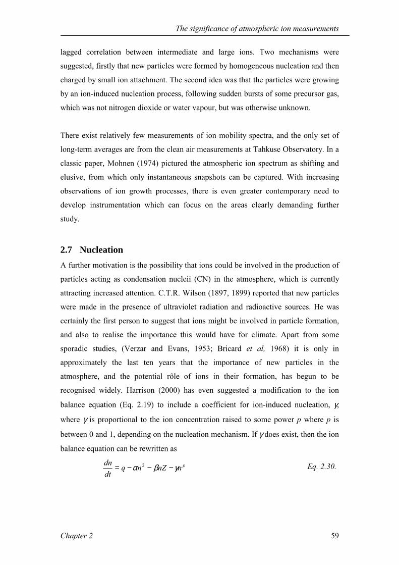
The significance of atmospheric ion measurements
Chapter 2 59
lagged correlation between intermediate and large ions. Two mechanisms were
suggested, firstly that new particles were formed by homogeneous nucleation and then
charged by small ion attachment. The second idea was that the particles were growing
by an ion-induced nucleation process, following sudden bursts of some precursor gas,
which was not nitrogen dioxide or water vapour, but was otherwise unknown.
There exist relatively few measurements of ion mobility spectra, and the only set of
long-term averages are from the clean air measurements at Tahkuse Observatory. In a
classic paper, Mohnen (1974) pictured the atmospheric ion spectrum as shifting and
elusive, from which only instantaneous snapshots can be captured. With increasing
observations of ion growth processes, there is even greater contemporary need to
develop instrumentation which can focus on the areas clearly demanding further
study.
2.7 Nucleation A further motivation is the possibility that ions could be involved in the production of
particles acting as condensation nucleii (CN) in the atmosphere, which is currently
attracting increased attention. C.T.R. Wilson (1897, 1899) reported that new particles
were made in the presence of ultraviolet radiation and radioactive sources. He was
certainly the first person to suggest that ions might be involved in particle formation,
and also to realise the importance this would have for climate. Apart from some
sporadic studies, (Verzar and Evans, 1953; Bricard et al, 1968) it is only in
approximately the last ten years that the importance of new particles in the
atmosphere, and the potential rôle of ions in their formation, has begun to be
recognised widely. Harrison (2000) has even suggested a modification to the ion
balance equation (Eq. 2.19) to include a coefficient for ion-induced nucleation, γ,
where γ is proportional to the ion concentration raised to some power p where p is
between 0 and 1, depending on the nucleation mechanism. If γ does exist, then the ion
balance equation can be rewritten as
pnnZnqdtdn γβα −−−= 2 Eq. 2.30.

The significance of atmospheric ion measurements
Chapter 2 60
The recent surge of interest in this subject could have been provoked by several
factors, for example unexplained observations of bursts of new particles in the
atmosphere (ODowd et al, 1996, Mäkelä et al, 1997). Theories of binary
homogenous nucleation, which is the classically assumed aerosol formation
mechanism (ODowd et al, 1996), also predict rates that are too slow to account for
observed aerosol concentrations (Yu and Turco, 2000; Kulmala et al, 2000). A
number of laboratory studies have shown that particles can be produced in the
presence of ionising radiation, although the findings are not concordant, and the
experiments often involved so much radiation that their results cannot be extrapolated
to atmospheric conditions. Climate models need to include aerosol particle source and
loss terms accurately to parameterise the radiative effects of the atmospheric aerosol
burden. Finally, the controversial theory relating the solar cycle to global cloud cover
suggests that ionisation contributes to particle formation without postulating a
microphysical mechanism (e.g. Svensmark and Friis-Christensen, 1997). Although
this has attracted considerable attention to the topic, in particular to rebutting their
theory, (a particularly recent example is Jorgensen and Hansen (2000)) little effort has
been made to prove or refute the microphysical aspects.
2.7.1 Nucleation onto ions Heterogeneous nucleation is the term used to describe the condensation of some
vapour onto a particle of a different composition to the vapour. When the particle is
an ion, the physics is quantified by the Thomson equation, which describes the
variation in the Gibbs free energy of molecules clustering around a nucleus. When the
Gibbs free energy ∆G is at a saddle point, particle growth becomes energetically
feasible. If r is particle radius, ρ the fluid density, S is supersaturation ratio, M the
mass of the molecule (in SI units), q particle charge, γT the surface tension, kB
Boltzmanns constant, T temperature, εr the relative permittivity and ro the initial
particle radius, the equilibrium condition for this situation can be written as:
−−=
r
T
B rq
rTkMS
εεπγ
ρ11
322ln 4
02
2
Eq. 2.31
which expresses the necessary conditions for nucleation in terms of a supersaturation
S (Mason, 1971). The presence of a charged central particle lowers the supersaturation
needed for condensation to occur. Wilson (1899) used his cloud chamber to measure
the supersaturations required for nucleation in the presence of radioactive sources (i.e.

The significance of atmospheric ion measurements
Chapter 2 61
almost certainly onto ions), which were in the range 250-370%, which is too high to
occur in the atmosphere. However, comparison with the greater supersaturations
needed for homogenous nucleation illustrates the way in which electrical charge can
stabilise cluster growth.
291.434767
0.02264
acid100 r( )
acid10 r( )
acid1 r( )
water100 r( )
water10 r( )
water1 r( )
1 10 6.4.6 10 10. r1 10 10 1 10 9 1 10 8 1 10 7 1 10 6
0.01
0.1
1
10
100
1 103
acid, 100eacid, 10eacid, 1ewater, 100ewater, 10ewater, 1e
radius (m)
supe
rsat
urat
ion
(per
cent
)
Figure 2.12 Equilibrium vapour pressure as a function of particle radius from Eq.
2.31, for droplets of water and sulphuric acid growing onto ions with different
elementary charges (at 300K). The saturation vapour pressure of sulphuric acid is
calculated from the expression in Laaksonen and Kulmala (1991). The surface tension
of sulphuric acid was assumed to be the same as water.
Figure 2.12 shows that increasing the charge stabilises droplets at lower
supersaturations. A water droplet can grow at atmospheric supersaturation levels
when it has a critical radius of about 5 nm and a charge exceeding about ten
elementary charges. This suggests that ions can act as nucleation sites for water
droplet growth, but since few particles in the atmosphere hold the necessary charge,
there is a low probability of this occurring. Ion-assisted nucleation of sulphuric acid is
possibly more likely because of its lower vapour pressure, and Figure 2.12 shows that

The significance of atmospheric ion measurements
Chapter 2 62
for greater than one elementary charge, sulphuric acid can be nucleated at lower
supersaturations than water. Typically, sulphuric acid exists in the atmosphere at
300K with a partial pressure of 10-4 mbar (Warneck, 1987) and in concentrations of
order 0.04 pptv (Kirkby et al, 2000). The saturation vapour pressure of sulphuric acid
at 300K is around 400 mbar, so any supersaturation in these conditions is highly
unlikely.
2.7.2 Laboratory observations of nucleation Bricard et al (1968) measured the number of new particles formed in clean air in a
chamber under the influence of ionising radiation, different trace gases and
illumination. They found the CN concentration could be made to cycle up and down
when regularly adding a short-lived source of α-particles (0.5 Bqm-3)20 on a five-
minute timescale, when the concentration of new aerosol varied by approximately a
factor of two (Figure 2.13). The radii of the new particles were estimated to be 2 nm
in the presence of the radiation, and 12 nm out of it. The smaller particles correspond
to the size of atmospheric small ions, which are produced in abundance by the
radioactive source. However, further measurements showed that only about 10% of
the total particle number was charged, indicating that in the presence of ionising
radiation an excess of neutral particles were produced. This suggests an ion-ion
recombination mechanism; but Bricard et al (1968) hypothesised that the coagulation
rate depended on the sulphur dioxide concentration, in the presence of some other
gaseous impurity.
Bricard et al (1968) also measured ion mobility spectra during the nucleation process,
finding a number of well-defined ion mobilities, which they matched to certain
species. Addition of SO2 caused the mean mobility to decrease, and the characteristics
of the mobility spectrum changed to a continuous shape, indicating ionic growth
processes. Application of Thomsons theory for heterogeneous nucleation gave a
critical radius, (the minimum radius of stable particles) of 0.7 nm if the mobility was
1 cm2V-1s-1 (corresponding to a typical atmospheric small ion of radius 0.5 nm
(Tammet, 1995)). It was suggested that the presence of sulphuric acid in the vicinity
of the droplets promoted nucleation by increasing the supersaturation. The
20 1 Becquerel = 1 decay per second

The significance of atmospheric ion measurements
Chapter 2 63
hypothesised physical growth mechanism (Bricard et al, 1968) was that the particles
grew because neutral nucleii of below the critical radius captured a charged particle to
stabilise and then grow. However, this does not explain Bricard et al's observations
(1968) of production of neutral particles in a radioactive environment.
Figure 2.13 The increase in particle concentration every time 10 rads21 of thoron, a
short-lived radon isotope, is introduced into a reaction chamber containing filtered
urban air likely to be high in sulphur dioxide and other trace pollutant gases (from
Bricard, 1968).
In the 1980s there was a resurgence of interest in the formation of aerosol particles in
the atmosphere. Increasing concentrations of the radioactive gas Krypton-85 from
nuclear fuel reprocessing generally encouraged research into the atmospheric effects
of ionising radiation. Observations of the environmental effects of acidic rainfall, and
21 The rad is defined by Handloser (1959) as the amount of radiation which results in the absorption of 100 ergs/gram of any material. Therefore it represents the energy imparted to the medium by the radioactive source. In SI units, 1 rad = 0.01 J/kg.

The significance of atmospheric ion measurements
Chapter 2 64
the depletion of forests near to nuclear installations, motivated studies of whether
radioactivity could be implicated in the production of sulphuric acid aerosol in
polluted (particularly SO2 laden) environments (Raes et al, 1985).
Consequently there were several laboratory studies attempting to simulate aerosol
production from ionising radiation, usually in air containing SO2, and a radioactive
source. Raes et al (1985) carried out experiments in synthetic air containing typically
0.015 ppm NO2 and 0.5 ppm SO2, with cobalt-60 (a γ-source) and ultra-violet
irradiation. They found that at the higher dose rates, γ-radiation could produce an
extra 105 particles cm-3, but at low dose rates, ultra-violet radiation was needed in
addition to the ionising radiation to produce any new aerosol particles. The threshold
activity was found to be 10-2 µGys-1 22, which is about three orders of magnitude
higher than natural background activity. This study is unrealistic for the atmosphere,
since γ-radiation is poor at ionising air and only contributes slightly to atmospheric
ionisation, and Raes et al (1986) conceded that their results were not applicable to the
atmosphere.
More recent work (Emi et al, 1998) contradicts both Bricard et al (1968) and
Diamond et al (1985) who reported that only neutral particles were produced from
ions. Emi et al (1998) describe results obtained with an ion mobility analyser, with an
americium-241 source in air containing 5 ppm SO2 and 3500 ppm water. They
observed a mobility peak at 0.1 cm-2V-1s-1, which clearly shows the presence of
charged particles of 1 nm radius (Tammet, 1995). This is suggestive of an ion growth
process, but since the particles formed are only intermediate ions (Hõrrak et al,
1998a) this provides no evidence of nucleation to larger aerosol particles. Adachi et al
(1998) measured the charged fraction in a mixture of NO2, ammonia (0.68 ppm),
water (3000 ppm) and air, in the presence of two 3.03 MBq americium-241 sources.
About 103 cm-3 new particles were produced after three minutes in the presence of
small concentrations of NO2, 80% of which were charged. This again suggests ion
growth is occurring, but no information regarding the size of the particles produced
was available.
22 1 Gray =1 J/kg.

The significance of atmospheric ion measurements
Chapter 2 65
Diamond et al (1985) suggest a mechanism whereby ions are not directly involved in
a chemical reaction to make sulphuric acid. Their mechanism involves an excited ion
transferring its energy to assist in SO2 oxidation, which then leads to nucleation.
Although they argue relatively convincingly for this mechanism given their
observations of the chemistry of different energy ions from different sources, they do
not address the fundamental question of whether the precursor ions are likely to meet
the energetic requirements for the reaction. Further research into the basic chemical
properties of air ions is clearly required for this line of enquiry to progress further.
The experiments of Vohra et al (1984) appear to be the only laboratory studies of
particle formation with levels of radioactivity naturally occurring in the atmosphere.
They used a radon source of 100-500 pCi m-3 (atmospheric concentrations are cited
by Vohra et al (1984) as 90-400 pCi m-3)23, and found that 7 x 10⁴ m-3 particles were
formed in their 4:1 nitrogen-oxygen mixture in the presence of SO2, ozone and
ethene, with radon present at the lowest atmospheric concentrations. Since Vohra et al
(1984) did not even mention ions in their discussions, it would be helpful for these
experiments to be repeated in conjunction with detailed ion measurements. A similar
experiment has been proposed at CERN to simulate atmospheric ionisation in a
controlled environment (Kirkby et al, 2000). This will be the first of its kind, since the
ionisation will be similar to that caused by cosmic rays, and may help to explain the
observations of Vohra et al (1984).
It would be useful to have an empirical expression for ion (or particle) production as a
function of radiation based on all these experiments. This is difficult because of the
different radioactive sources and units used. In terms of ionisation, the units of
Roentgen and Becquerel appear favourable to describe radiation, since Roentgens are
defined explicitly in terms of ionisation in air: 1 Roentgen is the dose of X or γ-
radiation such that the emission per 0.001293g of air produces 1 e.s.u. of electric
charge (Handloser, 1959). In modern units, 1 Roentgen is equivalent to 208230 ions
m-3, or 8.7 mGy in air. The Roentgen is rarely used now because of its irrelevance to
health physics, and the ionisation in air is only defined in terms of X and γ-radiation,
which are not the major sources of air ions. The Becquerel is defined as one decay per
23 1 Curie = 3.7 x 10¹⁰ Bq

The significance of atmospheric ion measurements
Chapter 2 66
second; a single radioactive source has a total activity, often defined in Bq, whereas
for a fluid a volume must also be quoted. The experiments described above use a wide
variety of sources, units and chamber volumes, not all of which are quoted to facilitate
the calculations necessary for comparisons.
The majority of ionisation at ground level is from α-radiation, which is effective at
ionisation in air (hence its short range), so all α-decays can be assumed to produce
ions. As the energy required to make an air ion pair is constant, the ion production
rate q should be directly proportional to the activity expressed in Becquerels at ground
level, because of the dominance by α-radiation. However, the relationship is likely to
vary with the type of ionising radiation, since the amount of energy given up by
different radioactive particles to ionisation varies greatly. Mäkelä (1992) discusses a
more generally applicable measure of ionisation, the G-value, which is the number of
ion pairs produced per 100eV of absorbed energy. This varies depending on the
species ionised, because of their varying ionisation energy.
Product G-value (number of pairs/100 eV)
N2+ 2.24
O2+ 2.07
H2O+ 1.99
Table 2.2 Number of ion pairs produced per 100 eV of absorbed energy for common
atmospheric species, from Mäkelä (1992).
A plot of the dose in Grays against q should also be linear, independent of the source,
since it is related the energy used in ionisation. The effectiveness (or not) of the
radioactive species in ionisation is accounted for, because by measuring absorbed
energy in a Geiger tube, this energy must have also been used in ionisation. As about
35.6 eV is required to ionise one molecule of air, an average value of G in air is 2.81
ions/100 eV.
2.7.3 Observations of nucleation in the atmosphere Observations of new particle production in clean air, or air otherwise depleted of CN,
for example in the marine boundary layer, have recently become available. These
typically show bursts of particles in the nanometre size range, which are first observed
in the morning and grow throughout the day. ODowd et al (1996) have observed

The significance of atmospheric ion measurements
Chapter 2 67
sudden increases in the CN concentration, in marine environments in Antarctica and
in the Outer Hebrides. During a particularly sudden nucleation burst in the Weddell
Sea, the CN concentration increased from 550 to 3500 cm-3 in 15 minutes,
corresponding to a nucleation rate of about 3 particles cm-3s-1 (though Antarctic
conditions are fairly unique in meteorological and biological terms). The CN
concentration was reported to decay in 3-4 hours after the bursts due to rapid loss
from mixing, advection and coagulation. This time scale is less than the time scale of
CN growing to CCN (≈ 50 nm). There were also regular observations of nucleation
bursts in the Outer Hebrides, where CN grew from < 8 nm to about 40 nm in
approximately an hour, then decayed rapidly in half that time. ODowd et al (1996)
were unable to suggest a mechanism for these events, but noted that at the Scottish
site, there were large kelp beds near the coast leading to enhanced levels of dimethyl
sulphide (DMS), a compound known to be significant in aerosol formation.
Mäkelä et al (1997) measured particles with radii from 1.5-250 nm with differential
mobility particle sizers at Hyytiälä, in Finnish pine forest. Unlike ODowd et al
(1996), particles were observed growing from 5-6 nm at a few nanometres per hour
continuously until the evening, when they were big enough to be subsumed into the
background aerosol. These events occurred during sunny days in spring and summer
when there was a large temperature difference between the morning and early
afternoon, and the relative humidity decreased consistently. On the days when
nucleation was observed, there was often a reversal of the vertical temperature
gradient when the stable nocturnal boundary layer broke down at 0800-0900. This
suggested that the particle formation events were associated with vertical mixing and
could have been produced at a different height to the measurements, although Mäkelä
et al (1997) were confident that the smallest particles were produced in situ, probably
because of their short lifetime. The origin of the particles could not be ascertained and
was not directly related to any measured soil conditions. Photochemical or biogenic
activity producing trace species was a possible cause, but photosynthesis was
discounted since it does not occur in Finland in early spring.
The significance of atmospheric ion measurements
Chapter 2 68
2.7.4 Models Mäkelä (1992) modelled the production of sulphuric acid aerosol in an irradiated
environment. His first step was to model the formation of ions from radioactivity
(assuming an aerosol-free environment, and that the dose rate distribution is
Gaussian). He expressed the change of ion concentration dn/dt in unit volume as
2)( ntGDdtdn αρ −= Eq. 2.32
where n is the ion concentration, G the number of ion pairs produced per unit of
absorbed energy, D the absorbed dose rate, ρ the gas density and α the self-
recombination coefficient.
y = 132802x + 2E+07R2 = 0.9976
y = 168107.62x0.64
R2 = 0.98
0.E+00
1.E+07
2.E+07
3.E+07
4.E+07
5.E+07
6.E+07
7.E+07
0 1000 2000 3000 4000 5000 6000 7000 8000 9000 10000
dose / µµµµGy
ion
conc
entr
atio
n /c
m-3
0.0E+00
2.0E+08
4.0E+08
6.0E+08
8.0E+08
1.0E+09
1.2E+09
1.4E+09
1.6E+09
ion
prod
uctio
n ra
te (c
m-3
s-1)
Ion pairs
Ion production rate
linear fit to q
power law fit to n
Figure 2.14 Ion concentration (n) (left axis) and ion production rate (q) (right axis)
as a function of dose rate. Shaded points are from Raes et al (1985, 1986), unshaded
points are from Mäkelä (1992).
Figure 2.14 shows the relationship between dose rate and ion concentration and
production rate, from values of n quoted by Raes et al (1985, 1986) and Mäkelä
(1992), which they calculated assuming the recombination limit (Eq. 2.20). The ion
production rate q, also calculated assuming the recombination limit (Eq. 2.20), shows
a good (R2 = 0.998) linear relationship with radioactive dose D. In the recombination
limit, D should be proportional to n2. The best power law fit between D and n gives
D ∝ n0.64, which shows that the recombination limit is a good approximation. The

The significance of atmospheric ion measurements
Chapter 2 69
recombination limit is not a perfect fit to the data, because Raes et al (1985, 1986)
reported aerosol production in their experiments (described in Section 2.7.2) so there
would have been attachment effects. This plot is not applicable to atmospheric air,
since the dose and ionisation rates are much higher than typical atmospheric
ionisation rates (2-10 ion pairs cm-3s-1).
Mäkelä (1992), empirically estimated sulphuric acid aerosol production as a function
of irradiation. From two sets of existing measurements, he was able to state that for a
total dose of 1mGy, if one ion is produced per 100eV this gives 8 x 10¹³ particles m-3.
He then measured the production of ultra-fine aerosol particles in a water-sulphuric
acid system in a chamber irradiated with 241Am. His results are shown in Figure 2.15.
Above a dose of about 0.4 mGy, the number of particles formed varied linearly with
respect to dose rate, with a gradient equivalent to the square root of the dose. This
implies that the particles are behaving as ions under the recombination limit, which
Mäkelä (1992) interprets as ion-induced nucleation of particles provoked by the very
high ion concentration. This hypothesis is supported by his observations of shifts in
the ion mobility spectrum towards larger sizes. The critical dose rate above which
the experimental results become linear is probably when there are enough ions present
for them to condense onto every sulphuric acid particle. Mäkelä (1992) also explains
that at high dose rates, the particle concentration becomes steady because of
attachment. These results are clearly inapplicable to the atmosphere, since the
chamber is so highly ionised that the recombination limit affects even the new
particles that are produced, and in the atmosphere the background aerosol would
modulate the ion production rate, probably to the extent that it never gets high enough
for ion-induced nucleation.

The significance of atmospheric ion measurements
Chapter 2 70
Figure 2.15 Results obtained by Mäkelä (1992). Ni,max (dotted line) is the ion
concentration calculated from the dose using the G-value and assuming the
recombination limit. Jion (filled circles) are model predictions for particles produced
from ion-induced nucleation. Jhom (crosses) are predictions for homogenous
nucleation. EMS (empty squares) are the results of Mäkeläs (1992) experimental
investigations, made at 20 °C, 15 % RH and 10ppm SO2.
A microphysical model of ions and aerosol including detailed electrostatic effects has
been used by Turco et al (1998) and Yu and Turco (2000) to show that ions in
atmospheric concentrations can facilitate production of sulphate aerosol by
nucleation. Sulphate was chosen for use in the model because from observations, it is
the most likely nucleating agent, and its thermodynamics is better characterised than
other potential nucleating agents such as organic compounds (Turco et al, 1998). The
microphysical model had previously been used to accurately predict particle
formation from ions in aircraft plumes (Yu and Turco, 1997). Though under these
conditions ion and sulphate concentrations are much higher than in the atmosphere,
these results indicate that the microphysics of ion-mediated nucleation is an existing
effect, which has been accurately parameterised in the aerosol model. The mechanism
suggested by Yu and Turco (2000) is one whereby the recombination of a hydronium
positive ion and a sulphate negative ion can produce a cluster that is larger than the

The significance of atmospheric ion measurements
Chapter 2 71
critical size for nucleation. This effect is strongly dependent on the sulphuric acid
concentration, with the degree of dependency varying non-linearly with the various
feedback mechanisms. Turco et al (1998) calculate that the nucleation rate Jnuc
depends on the sulphuric acid concentration [H2SO4] raised to some power n, where
the constant of proportionality accounts for the ionisation rate
[ ]nnuc SOHJ 42∝ Eq. 2.33.
The magnitude of n is related to the number of ligands that are required to stabilise a
neutral recombination product, and will vary according to the temperature and relative
humidity. A secondary mechanism is that the electrical charge held by an ion cluster
can also enhance the probability of a collision with a molecule of sulphuric acid by an
order of magnitude (Yu and Turco, 2000).
In Yu and Turco (2000) the model is tested by applying similar code to the initial
conditions for observations of particle formation from air ion mobility spectra at
Tahkuse Observatory (discussed above), and also measurements of ultrafine aerosol
and sulphuric acid made in Colorado. In both cases the model accurately predicts
similar results to the experiments. However, the effects of background aerosol are
ignored which meant that to get ion concentrations comparable with those measured
at Tahkuse, the surface ionisation rate had to be set at a value which is comparable to
the cosmic ray contribution only. Rather than scaling q to 2 cm-3s-1 to arrive at
n = 1000cm-3, it might be better to retain a more typical atmospheric value of q =
10cm-3 s-1 (Chalmers, 1967). In this case, assuming a steady-state variation and using
2
nnqZ
βα−= Eq. 2.34.
(Clement and Harrison, 1992) there should actually be an associated pre-existing
monodisperse aerosol concentration of Z ≈ 1000cm-3, using an ion-aerosol attachment
coefficient β typical of a 0.2 µm radius aerosol. This presence of the background
aerosol particles is particularly important because they can also remove the necessary
condensable vapour, cutting off the nucleation (Harrison and Aplin, 2000b). It is interesting that Yu and Turcos (2000) model should match the Estonian results
so well, since their ion-ion recombination mechanism suggests that neutral particles
should be produced, and in this case there would be no progressive shift in the

The significance of atmospheric ion measurements
Chapter 2 72
mobility spectrum. This implies one of two things; either that the enhanced
coagulation onto charged particles is actually more significant than their model
suggests, or secondly that the sulphuric acid concentrations (which were not measured
at Tahkuse) were selected so as to give results which fitted the observations best. The
second set of results the model was compared are more appropriate since neutral
particles were measured as well as sulphuric acid.
Kulmala et al (2000) propose a different mechanism, which has also had some
success in explaining experimental observations. They have modelled a ternary
nucleation system, of sulphuric acid, ammonia and water, which predicts nucleation
under typical tropospheric sulphuric acid concentrations. Other suggested
mechanisms tend to rely on transiently high supersaturations of sulphuric acid for
nucleation, which are both unproven and difficult to measure. They suggest a model
where there are reservoirs of thermodynamically stable clusters (TSCs) which are too
small to detect (< 1nm), and certain conditions will trigger their growth to resolvable
sizes, which is when a nucleation burst occurs. The detectable TSC concentration is
dependent on the existing aerosol concentration; when this is high the TSCs are lost
by coagulation to larger aerosol particles. The sulphuric acid concentration is also
important and nucleation rates are about a thousand times slower than in binary
nucleation because of the lower concentrations required. If, however, air containing
TSCs is advected over a mass of a source of condensable species (for example,
photochemically produced organics) this can produce a burst of larger particles which
can continue to grow to the sizes detected by Mäkelä et al (1997). In Kulmala et al
(2000), their ternary nucleation model is applied to the preliminary conditions for
nucleation at Hyytiälä in Finland and matches the observations well. It does not
appear to be possible to test this model properly until aerosol instrumentation that can
measure particles in the 1-3 nm size range is available. This nucleation mechanism,
however, does not invoke ions, unlike Yu and Turco (2000) and Hõrrak et al (1998a,
2000), since the TSCs are neutral particles and for there to be charge equilibrium with
the background small ion concentration, only a tiny fraction could be charged.
Kulmala et al (2000) firmly rule out ion-induced nucleation because their ternary
nucleation mechanism (in conjunction with advection of condensable vapour) occurs
at rates of 50-100 cm-3s-1, which considerably exceeds average atmospheric ionisation

The significance of atmospheric ion measurements
Chapter 2 73
rates. However, the ionisation rate can vary considerably (Harrison, 2000) and it is
possible that short-lived transients caused by highly energetic particles could cause
the ionisation rate to peak for long enough to push the TSCs into the detectable size
range.
There is a well-established body of evidence that ionising radiation can result in the
production of fine particles. Additionally, it seems probable that ions are implicated in
this process. However, the paucity of experimental atmospheric observations of ions
and particle formation, and lack of a plausible theoretical basis has meant that
experimentation has not been directed towards investigating ions and atmospheric
nucleation. Only very recently have microphysical simulations suggested nucleation
mechanisms feasible in atmospheric conditions.
2.8 Conclusions The two differing theories of atmospheric aerosol formation, both of which have
successfully explained aspects of existing experimental data, now provide a very
strong motivation to measure air ion mobility spectra. In one of these theories, ions
are crucial, and accurate measurements of the atmospheric ion spectrum are clearly
required to corroborate or refute. There is no reason why both the mechanisms
proposed by Kulmala et al (2000) and Yu and Turco (2000) cannot apply under
different conditions, but further investigations of ultrafine aerosol particles, in
conjunction with meteorological, electrical and chemical measurements will be
required to differentiate between them.
At the moment, the instrumentation required to test the hypothesis that ions are
involved (by whatever mechanism) in CN production is not available. Instruments to
measure ion mobility spectra have been developed and deployed, but there are often
play-offs between mobility and time resolution, and fundamental assumptions about
the nature of the ion spectrum. Instrumentation developed to date has usually had its
time and mobility resolution rigidly fixed at the outset as a consequence of its design,
although suitable operating conditions may only be known after observations have
been made. The classical Gerdien instrumentation also fundamentally lacks a viable
calibration technique, despite the availability of an alternative mode to check self-

The significance of atmospheric ion measurements
Chapter 2 74
consistency. There is a pressing need for a flexible and portable instrument that can be
utilised for a variety of purposes.
A miniaturised Gerdien device
Chapter 3 75
"In order to make it work, you had to spit on the wire in some Friday evening in Lent" Patrick Blackett24
3 A miniaturised Gerdien device
In this chapter, an ion counter based on the classical cylindrical capacitor designed by
Gerdien (1905) is analysed in terms of its separate components. Firstly, some
semantics are required to differentiate the components of the ion counter. The term
Gerdien tube eponymously refers to the part of the instrument which replicates
Gerdiens, i.e. the central and outer cylindrical electrodes. Gerdien condenser is
used to describe the capacitative properties of the Gerdien tube. The instrument
described here differs from the classical Gerdien device in that it includes a third,
screening electrode, and here this configuration is simply called a Gerdien.
Gerdien system refers to the complete instrumentation necessary to measure ions,
which consists of the Gerdien, associated electrometer and bias voltage supply.
The objectives of the chapter are to attain a detailed knowledge of the Gerdien system
components, and to test the instrument in atmospheric air. The physical properties of
the tube and the flow through it, and the measurement systems are all examined in
terms of setting design criteria (Section 3.1), and their direct application to making
measurements in the atmosphere (Section 3.2). Some measurements are made with
the Gerdien system in air in Section 3.3. They are tested against theoretical
predictions, and for self-consistency.
3.1 Design criteria
3.1.1 Tube material and dimensions The critical mobility defines the minimum mobility of ion which contributes to the
measurement (see Eq. 2.11) and is the single most important Gerdien design
specification. The instrument dimensions need to be chosen so that the critical
mobility, given the tube voltage and airflow rate, is an appropriate value for
measuring atmospheric ions. Since typical ion mobilities ≈ 10-4 m2V-1s-1, the critical
mobility needs to be of this order of magnitude for conductivity measurement (see
24 (about the Geiger tube). This quotation was on display at the Science Museum in April 2000.

A miniaturised Gerdien device
Chapter 3 76
Section 2.2.2). If the Gerdien is to be used as an ion mobility spectrometer, the tube
dimensions need to be chosen so that a realistic voltage range will investigate the
desired part of the mobility spectrum. Exact details will depend on the context, for
example the ion size range to be investigated. Limitations to the bias voltage supply
are also significant: large voltages are difficult to switch and control accurately, being
prone to ripple (Harrison, 1997b).
If the critical mobility is low enough so that the vast majority of the air ions are
collected, there is no change in conduction current with voltage. This is the flat region
on Figure 3.1, known as saturation, when the Gerdien only counts the total number of
ions. Outside the saturation region there should be an approximately Ohmic
relationship between bias voltage and measured current, depicted as the straight line
in Figure 3.1. To see a true Ohmic relationship there would need to be a unimodal ion
mobility spectrum; in reality, changes in the mobility spectrum cause slight variations
in the conductivity at different voltages (as mentioned in Section 2.2.2). The best way
to maintain Ohms law is to ensure the Gerdien is sufficiently ventilated, since the
critical mobility is directly proportional to the flow rate (MR, 1998).
Ohmic
Cur
rent
i
Bias voltage V
Saturation
Figure 3.1 Idealised i-V relationship for a Gerdien condenser, showing the two
operating régimes (after Chalmers, 1967).
In Chapter 2, tube material was discussed briefly. The literature suggests no scientific
reasons to prefer one metal in particular, although it seems sensible to start with a
material that has previously been used successfully. Aluminium tubes were used by
Hatakayema et al (1958) and Venkiteshwaran (1958), and for the Gerdien tested in
this chapter, aluminium was initially chosen for the outer electrode because of its
workability. The central electrode was made of stainless steel wire. A second
aluminium cylinder, which was earthed, was used as a screen to reduce

A miniaturised Gerdien device
Chapter 3 77
electromagnetic interference. The outer electrode and screen were insulated from each
other with a PVC separator. The tube dimensions are tabulated below, and Figure 3.2
is a simplified diagram of the system.

A miniaturised Gerdien device
Chapter 3 78
Figure 3.2 Schematic diagram of the Gerdien system in Current Measurement mode.
BNC B supplies the bias voltage. BNC A measures the ion current, and its outer
connection is driven by the current amplifier.
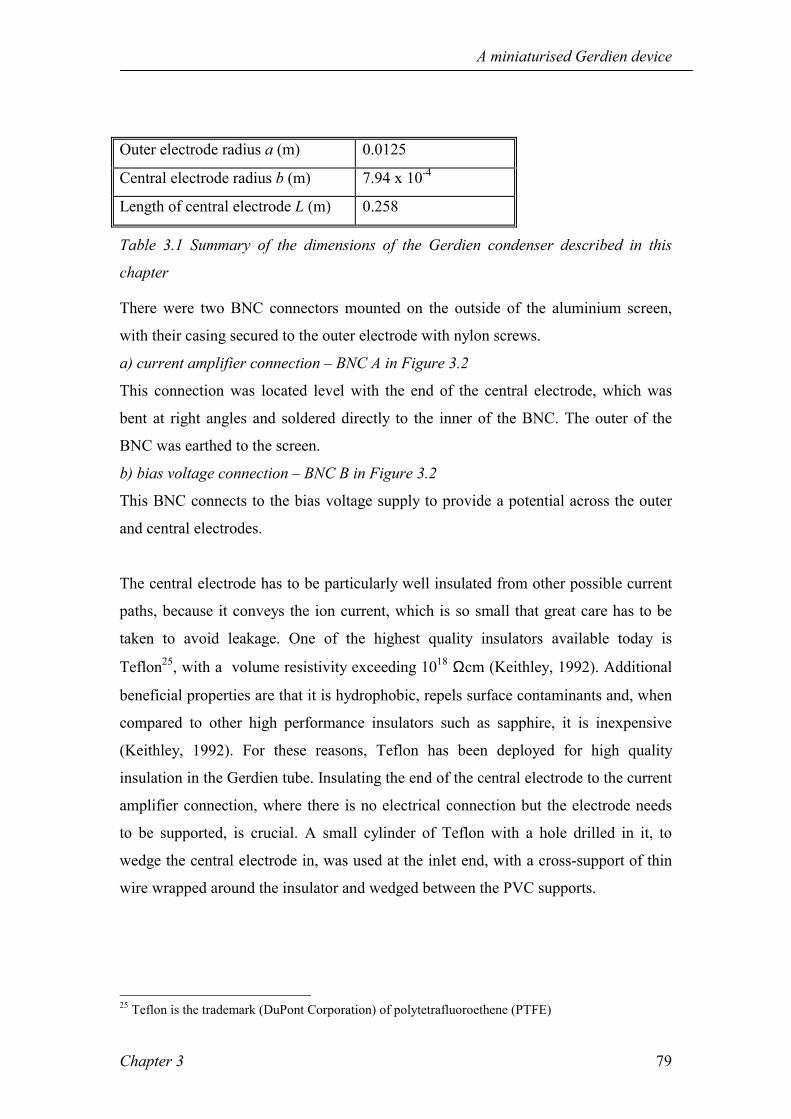
A miniaturised Gerdien device
Chapter 3 79
Outer electrode radius a (m) 0.0125
Central electrode radius b (m) 7.94 x 10⁻⁴
Length of central electrode L (m) 0.258
Table 3.1 Summary of the dimensions of the Gerdien condenser described in this
chapter
There were two BNC connectors mounted on the outside of the aluminium screen,
with their casing secured to the outer electrode with nylon screws.
a) current amplifier connection BNC A in Figure 3.2
This connection was located level with the end of the central electrode, which was
bent at right angles and soldered directly to the inner of the BNC. The outer of the
BNC was earthed to the screen.
b) bias voltage connection BNC B in Figure 3.2
This BNC connects to the bias voltage supply to provide a potential across the outer
and central electrodes.
The central electrode has to be particularly well insulated from other possible current
paths, because it conveys the ion current, which is so small that great care has to be
taken to avoid leakage. One of the highest quality insulators available today is
Teflon25, with a volume resistivity exceeding 1018 Ωcm (Keithley, 1992). Additional
beneficial properties are that it is hydrophobic, repels surface contaminants and, when
compared to other high performance insulators such as sapphire, it is inexpensive
(Keithley, 1992). For these reasons, Teflon has been deployed for high quality
insulation in the Gerdien tube. Insulating the end of the central electrode to the current
amplifier connection, where there is no electrical connection but the electrode needs
to be supported, is crucial. A small cylinder of Teflon with a hole drilled in it, to
wedge the central electrode in, was used at the inlet end, with a cross-support of thin
wire wrapped around the insulator and wedged between the PVC supports.
25 Teflon is the trademark (DuPont Corporation) of polytetrafluoroethene (PTFE)

A miniaturised Gerdien device
Chapter 3 80
The insulated end of the central electrode is at the Gerdien inlet. It is important that
the disturbance to the air entering the tube is minimised to reduce turbulence, whilst
ensuring charge does not accumulate on the insulator and perturb the electric field at
the inlet. For these reasons, an electrically floating metallic cap with rounded edges in
a bullet shape was attached to the insulator at the end of the central electrode to
protect it, whilst keeping the flow into the tube as smooth as possible.
3.1.2 Flow rates The critical mobility (derived in Section 2.2.2) is determined by the ratio of flow rate
u and bias voltage V such that
Vukc =µ Eq. 3.1.
where k is a constant (with dimensions of length) related to the physical dimensions of
the tube: outer electrode radius a, central electrode radius b and tube length L, as
( )L
baba
k2
ln22
−=
Eq. 3.2.
As can be seen from Figure 3.3, the critical mobility varies considerably with V and u.
The flow rate and bias voltage therefore need to be selected in order to measure the
required critical mobilities. It is clear that some source of external ventilation is
required to prevent the tube saturating and operating in the ion counter mode for
periods of low wind speeds, for example during testing in the laboratory. The bias
voltage has to be chosen once the average flow in the tube has been estimated.

A miniaturised Gerdien device
Chapter 3 81
0.0
1.0
2.0
3.0
4.0
5.0
0 20 40 60 80 100 120Bias voltage(V)
µµ µµ c x
10-4
m2 V-1
s-1
u = 3 m/su = 1.5 m/s
Figure 3.3 Critical mobility µc against bias voltage at two flow rates for
k = 0.00178 m, the value used in the Gerdien experiments discussed in this chapter.
For the Gerdien used here, a small electric fan in a cylindrical plastic casing26 was
inserted in one end of the tube to ventilate it. If the polarity is reversed when
connecting it to the supply, air can alternatively be sucked through the tube, passing
through the fan after the electrodes. This is preferable to measurements being made
from air that has already been disturbed by the fan. Previous conductivity
measurement do not always state the direction of ventilation, but since many of them
had the Gerdien located inside a building or at a window, they would have needed to
suck air through the tube (e.g. Higazi and Chalmers, 1966).
The flow rate in the Gerdien was measured with a hot wire anemometer27 inside a
cardboard tube of similar dimensions to the Gerdien, ventilated with the fan. A 12V
supply gave a flow rate of about 2.2 ms-1. The bias voltages were selected based on
this, using a reversible, variable voltage supply constructed from ten 12 V batteries to
provide Gerdien voltages in the range 12-120 V with a ten-way switch. This was
26 12 V dc, ~ 40 mA, RS components part no. 600-904 27 Testo 435 meter, measures to ± 0.1 ms-1

A miniaturised Gerdien device
Chapter 3 82
connected to the outer electrode via a BNC connector on the tube. When smaller
voltages were needed, a battery or millivolt calibrator could be used.
Chalmers (1967) explains the need for Ohms Law to apply in conductivity
measurements, as a way of ensuring that the ion current never totally depletes the ion
concentration in the air near the electrodes. Chalmers (1967) defines a criterion to
maintain Ohms Law: the streamlines of the fluid flow (in this case, the fluid referred
to is ionised air) in a ventilated tube must be parallel to the electrodes, which implies
that the flow must be laminar (Tritton, 1988). Otherwise, Chalmers (1967) believes
the decay of charge from the condenser may not follow the classical exponential
formation in Eq. 2.3, from which the conductivity by the Voltage Decay method and
direct current measurement can be derived28. Perfectly laminar flow will be difficult
to maintain in a Gerdien tube, because of the ventilation requirement. The transition
to turbulent flow (i.e. random and chaotic fluctuations of turbulent eddies in the fluid)
can be defined in terms of the Reynolds number, Re, which is given by
η
ρ suL=Re Eq. 3.3
(e.g. Tritton, 1988) where ρ is the fluid density, η the fluid viscosity, Ls a
characteristic length scale and u the mean flow speed. Since turbulence starts to occur
at Re ∼ 103, then for a Gerdien of comparable dimensions to the one used here (length
25 cm, radius 2 cm), the flow will be turbulent for speeds exceeding about 0.1 ms-1,
which are likely to be insufficient to measure conductivity. Chalmers (1967) criterion
therefore seems approximate.
Consider the motion of ions in the tube; in a perfectly laminar flow they will be
subject to two forces only. An electrical force will act towards the central electrode,
and the mean flow will blow the ions along the tube. In turbulent flow there is a third
effect from the action of turbulent eddies, which introduce a chaotic aspect into the
ionic motion. As long as the mean flow exceeds the scale of the turbulent eddies, the
ionic motion predicted by theory (resulting most importantly in the critical mobility
Eq. 2.11) should still hold. In terms of the design of a Gerdien condenser, the
28 An alternative and perhaps more intuitive derivation is usually used for the Current Method, described in Section 2.2.2

A miniaturised Gerdien device
Chapter 3 83
condition of laminar flow imposed by Chalmers (1967) can be relaxed, as long as it
can be proved that the mean flow exceeds the motion due to turbulent eddies.
3.1.3 Measuring the ion signal Eq. 2.17 gives the relationship between ion current i, Gerdien bias voltage V and
capacitance C as
CV
ioεσ = Eq. 3.4.
If typical values of atmospheric conductivity are 10 fSm-1, the Gerdien bias voltage is
20 V and its capacitance is 10 pF, then substituting into Eq. 2.17 suggests that typical
Gerdien currents from an instrument of that specification will be ~ 200 fA in
magnitude29. The small magnitude of these currents implies that a specialist
electrometer is necessary. Commercially available instruments exist with resolution of
1 fA, such as the Keithley 6512, but these are bulky and expensive calibration devices
unsuited to fieldwork. When measuring such small currents, effects often considered
negligible in other circumstances are comparable to the signal, such as leakage
currents, and also the 50 Hz interference caused by the ac mains supply. Great care
therefore has to be taken to minimise these problems whilst maximising the time
response, by careful design and component selection, as in the current amplifier
developed by Harrison (1997a).
Measurement of the change in voltage across the Gerdien electrodes when the charge
on them decays through air is more straightforward, and a simple follower circuit can
minimise leakage currents if a suitable op-amp is chosen. However, the currents
flowing are clearly no larger than when they are measured directly at the central
electrode, and in the Voltage Decay mode, particular attention has to be paid to the
connections from the tube to the follower input to avoid leakage. This can be avoided
by driving the screen of the input at the output potential, a method known as guarding
(Horowitz and Hill, 1994).
29 Although Gerdiens used in the literature have varied considerably in size, their capacitance is usually of order 10 pF (e.g. Arathoon, 1991; Blakeslee and Krider, 1992). Consequently, the currents are usually dependent on the magnitude of the bias voltage, which is chosen based on critical mobility considerations, indirectly related to the size of the instrument through the constant k defined in Eq. 3.4. Since the Gerdien used here is smaller than average, this results in smaller output currents than measurements with larger Gerdien condensers.

A miniaturised Gerdien device
Chapter 3 84
A current amplifier is an instrument to measure a small current (Keithley, 1992) by
converting it into a voltage, which is usually linearly related to the input current30.
The simplest form of i-to-V converter is a resistor: for example, currents of 1 pA
could be converted into 1 V by passing them through a high value resistor of 1 TΩ.
However, a resistor is not ideal for current measurement because its time response is
limited by the time constant of the resistor and its own capacitance (typically a few
pF). With the high value resistors of order 1 TΩ required to measure small ion
currents, this immediately implies a time response of order seconds.
An alternative approach is to utilise the properties of operational amplifiers. The
output voltage of an op-amp is proportional to the potential difference at the inputs,
with the constant of proportionality given by the gain (Keithley, 1992). In conjunction
with a fixed resistance, operational amplifiers can also be used to convert current to
voltage. There are two configurations in which op-amps can act as i-to-V converters,
shunt and feedback31.
Vo
RF
RA
RBRS
i
i
a) Shunt ammeter b) Feedback ammeter
-+ -
+
Figure 3.4 Ammeters using op-amps, after Keithley (1992). RF and RS are the large
value resistors. i is input current, Vo is output. Note that for the shunt ammeter (a), the
signal joins the non-inverting input, and for the feedback ammeter (b), the inverting
input.
In the shunt ammeter (Figure 3.4a), the output voltage Vo is given by the expression
for a non-inverting amplifier with an input voltage iRs, i.e.: 30 It is also possible to make a logarithmic current amplifier (Keithley, 1992) by using a logarithmic feedback element. They are well suited to measuring currents in a wide range, for example atmospheric point discharge currents in fair weather and thunderstorms.

A miniaturised Gerdien device
Chapter 3 85
)1(
B
Aso R
RiRV += Eq. 3.5.
In the feedback ammeter (Figure 3.4b), the output voltage is related to the current i by
Fo iRV −= Eq. 3.6.
(Keithley, 1992). The shunt ammeter suffers from a similarly limited time response to
the resistor described above because the input capacitance and any stray capacitance
are in parallel with the shunt resistor RS (Arathoon, 1991). The feedback ammeter is
preferable because the op-amp's high gain means that negative feedback keeps the
inverting input as a virtual earth. As the non-inverting input is grounded, the voltage
across the inputs is very small so there is virtually no input capacitance, and the time
constant is only limited by the feedback resistor RF and its stray capacitance.
The feedback current amplifier used in this application was developed by Harrison
(1997a). It was designed specifically for atmospheric current measurements, and
incorporates a 30dB 50 Hz noise-rejection feature which uses a tuned filter to extract
the 50 Hz signal, phase-shift it by 180°, and feed it back to the input to cancel it out. It
also includes several features to minimise leakage currents; the input connection is
soldered directly to the op-amp inverting input. Harrison's (1997a) original current amplifier design had a feedback resistor of 1 GΩ.
Initial measurements showed that the Gerdien currents measured in the laboratory
were smaller than expected, probably due to ion-deficient indoor air. One possible
solution would be to add a further op-amp with gain A to increase the total sensitivity
of the system
)( FiRAV −= Eq. 3.7.
depicted in Figure 3.5. If A = -100, and RF = 1 GΩ, then the output is nominally
1V/pA. Another approach, which has the same overall effect on the gain, would be to
increase the feedback resistor to 1 TΩ, omitting the second gain stage or having A = -
1. "Gain trimming" is the process of adjusting A to get the desired response.
31 The feedback amplifier is sometimes also called the transresistance amplifier.

A miniaturised Gerdien device
Chapter 3 86
A
Vo
RF
IIN-
+
Figure 3.5 Feedback current amplifier including gain stage A
The principal difference between the two options is one of temperature stability. In
practice, there exists an input offset voltage Vos, which is a consequence of the
potential across the terminals of the input amplifier not being exactly zero; Vos is
defined as the voltage required at the input to cancel it at the output (Keithley, 1992).
There is also an input bias current iB which is defined as the average of the input
currents with the inputs shorted together. Physically, the input currents result from the
base leakage currents of the input transistors (Horowitz and Hill, 1994). The effects of
input offset voltage and input bias current are both magnified by the second op-amps
gain A, thus the total response V0 of the system is:
( ) [ ]osFB VRiiAV ++−=0 Eq. 3.8
RF, iB and Vos all have a temperature dependence, with higher value resistors being
more variable with temperature. (Resistor temperature dependencies are shown in
Table 3.2 below, where it can be seen that a 1 TΩ resistor is 70 % more temperature
sensitive than a 1 GΩ resistor.) The change in the output voltage ∆V for a finite
change in temperature ∆T can be written as:
( )
∆∆
+
+
∆∆
=∆∆
TV
iiTR
ATV os
Bf Eq. 3.9
There is thus a compromise between using a 1 GΩ resistor with a larger gain stage
magnifying the input offset voltage, and the 1 TΩ resistor with its greater temperature
dependence but no multiplication of Vos. The change of input bias current with
temperature has exactly the same effect on the output voltage in both cases, which is
discussed separately below. For the MAX406 operational amplifier,

A miniaturised Gerdien device
Chapter 3 87
∆Vos/∆T = 10 µV/ºC. The temperature coefficient of resistance for resistors from 109-
1012 Ω was obtained from the manufacturers information32, shown in Table 3.2.
Rf (ΩΩΩΩ) Temp coeff
of resistance
(/ºC)
∆∆∆∆Rf/∆∆∆∆T (ΩΩΩΩ /ºC) Gain A to
keep output
1V/pA
109 0.0010 106 1000
1010 0.0012 1.2 x 10⁷ 100
1011 0.0015 1.5 x 10⁸ 10
1012 0.0017 1.7x 10⁹ 1
Table 3.2 Resistance values, temperature coefficients and gains
The temperature sensitivity of the output voltage was calculated for different values of
feedback resistance, varying the gain to keep the response nominally 1V/pA, by
substituting data from Table 3.2 into Eq. 3.9 above. Figure 3.6 shows that increasing the value of the feedback resistor decreases the
overall temperature sensitivity of the current amplifier. With the 1 GΩ feedback
resistor, the term where the input offset voltage is multiplied by the gain in Eq. 3.9
dominates, with the error increasing for smaller currents. For larger resistors, the first
term in Eq. 3.9 dominates, improving the overall thermal stability despite the greater
sensitivity of the larger resistors to temperature changes.
32ELTEC Type 104, L.G. Products Limited, Slough (1994). (Now distributed through LGP Electro-optics, Chobham, Surrey.)

A miniaturised Gerdien device
Chapter 3 88
0%
10%
20%
30%
40%
50%
1.E+09 1.E+10 1.E+11 1.E+12RF / Ohms
Perc
enta
ge c
hang
e in
typi
cal s
igna
l per
deg
C 0.02 pA0.20 pA1.00 pA
Figure 3.6 Temperature sensitivity of the output voltage with Rf for typical input
currents from atmospheric ions (shown in pA in the legend), calculated from Eq. 3.9.
Comparisons were made of the temperature stability of a current amplifier using a
1 TΩ feedback resistor with two different electrometer grade op-amps:
• AD549JH (which has the ∆Vos/∆T = 10 µV/ºC as the MAX406), which was used
successfully by Arathoon (1991) in a feedback current amplifier with a 100GΩ
feedback resistor.
• MAX406, used in the Harrison (1997a) current amplifier.
Using the AD549JH compared to the MAX406 would reduce the input bias current at
0 °C by an order of magnitude, but increase it by a factor of two at 30 °C. Since the
two op-amps are otherwise similar, the more consistent value of iB is preferable as it is
easier to quantify. Following the analysis of temperature dependencies of input bias current and input
offset voltage, the MAX406 op-amp was unchanged from the original design
(Harrison, 1997a), but the feedback resistor was changed to a 1 TΩ with the second
stage having a gain of -1.

A miniaturised Gerdien device
Chapter 3 89
The thermal stability of the current amplifier's leakage terms were tested by logging
its output when its input was capped, at the Reading University Meteorology Field
Site. In this configuration, the output is from the combination of the input bias current
and leakage currents from the current amplifier, and shows a clear temperature
dependence which can be seen in Figure 3.7. The predicted effect of changes in
temperature on the input bias current alone is plotted in Figure 3.8. Although the
MAX406 has a small input bias current compared to other op-amps, if typical ion
currents are about 200 fA, then the input bias current introduces an error of about 5 %,
and in indoor tests this will probably be worse because of the higher temperatures and
smaller ion concentration.
-8.0
-7.5
-7.0
-6.5
-6.0
-5.5
-5.0
-4.5
-4.00 2 4 6 8 10 12 14 16 18 20
Mean temperature (deg C)
Mea
n (le
akag
e +
inpu
t bia
s) c
urre
nt (f
A)
Figure 3.7 Daily mean leakage current and temperature for March 1998, calculated
from automatically logged five minute averages of capped current amplifier output (in
volts) and temperature.

A miniaturised Gerdien device
Chapter 3 90
0
2
4
6
8
10
12
14
-10 -5 0 5 10 15 20 25 30
Temperature (deg C)
Inpu
t bia
s cu
rren
t(fA)
Figure 3.8 Variation of the typical MAX406 input bias current with temperature (from
manufacturers data sheet).
Both these effects will vary with the individual op-amp used, and Figure 3.8 in
particular is likely to be the worst case scenario quoted by the manufacturer.
However, it is clear that the temperature dependence of both the input bias current and
the electrometer leakage current are significant effects when measuring at the
femtoampere level. The observed current amplifier resolution of ± 3 fA at 20 ºC 33,
concurs with the trend in the sum of leakage and input bias currents shown in Figure
3.7, but the results suggest the leakage currents will be greater at lower temperatures.
The atmospheric results (measured at 2 12 ºC) support this; because ib is positive,
then the leakage currents in the circuit must be dominant to make the overall response
negative.
3.1.4 Switching devices in electrometry When a switch is required, for example in the Voltage Decay method to control the
bias voltage, great care has again to be taken to avoid leakage currents by choosing
well-insulated components. For this reason, sub-miniature glass encapsulated reed
33 This will be discussed further in section 3.2.3

A miniaturised Gerdien device
Chapter 3 91
switches34 in a activating electromagnetic coil35 were used for low leakage switching
applications. For the Gerdien system, the major applications were shorting out the
current amplifier's feedback resistor, and controlling the voltage which charges the
electrodes. This reed relay, cycling at 0.1 Hz, was used to short out the feedback resistor in the
current amplifier, with its input floating and screened. When the relay opened there
was a voltage transient of about 30 mV (corresponding to a negative charge injection
of ~ 6 fC) into the system. This exhibited a RC decay with a settling time of
approximately 5 s. Brownlee (1973) observed a similar 20 mV transient with the ERG
type MA/GO/J reed relays he was using to switch between connections to his
electrometer. To test whether this effect was a property of the relay he compared the
voltage transients using different capacitor values across the reed relay. From Eq.
(2.5), if q does not vary with time, then doubling the capacitance should halve the
voltage transient. Brownlee (1973) concluded from this that his relays injected a
charge of about 20 fC into the system. This confirms suspicions that the reed has a
small capacitance, and discharges when closed, which can cause transients36. To avoid
this charge injection affecting the current measurements, a suitable decay time should
be allowed to elapse after the relay switching, before making a measurement.
Another test of the reed relay, when connected across the current amplifier feedback
resistor, was to subject it to step changes in input current when it was fixed either on
or off, and observe the effect on its switching capabilities. When the relay was open,
changes in the input current greater than from +1 to 1 pA could cause it to jam in the
off (open) position. A possible explanation for this could be that as the op-amp is
inverting, the feedback voltage is of the opposite sign to the input current, but at the
instant when the sign of the input current is changed, the input and the feedback
potentials on the reeds are the same sign. The repulsion between the reed and its
input means that there is nowhere for the charge on the relay to dissipate to, which
could cause it to stick open. This would probably be an insignificant problem in
atmospheric measurements, because step changes of order 2 pA with a change of sign,
34 RS type 229-3658 35 RS type 349-844 36 An example of this is described in Section 3.3.1.
A miniaturised Gerdien device
Chapter 3 92
caused by ions are extremely unlikely. However, this effect might compromise the
long-term reliability of the relay switching.
3.2 Characterisation of individual components of the Gerdien
system In this section, the individual components of the Gerdien system are investigated.
Some wind tunnel experiments to identify the flow régime in the tube were carried out
and are described in Section 3.2.1. The findings of the flow investigation suggest that
fluctuations in the external ventilation may be important, necessitating further
consideration of its effects on the size of ions contributing to the measurement in
Section 3.2.2. The measurement system has also been studied in detail, and the
findings are presented in Section 3.2.3.
3.2.1 Flow properties of air in the Gerdien tube The aim of the experiments described in this section were to determine some
characteristics of the flow in the Gerdien tube, in particular how the flow in the tube
varied with the nature of the external flow. It is also necessary to confirm that flow in
the tube is approximately laminar, so classical Gerdien theory (Chalmers, 1967)
would apply (as discussed in Section 3.1.2).
The flow properties of the tube were investigated by making measurements with a
Disa type 56C01 hot-wire anemometer in a wind tunnel. The tube used was physically
identical in dimensions and composition to a Gerdien condenser, but lacked the
electrical connections. Measurements were made when the external ventilation was
sucking air through the Gerdien in the same direction as the fan, and also when the
external and induced ventilation (from the fan) were opposed. The probe was inserted
33.5 mm into the Gerdien, to measure the flow adjacent to the central electrode.

A miniaturised Gerdien device
Chapter 3 93
Pitot tube
Centralelectrode
Disa probe,inserted intoGerdien tube
Figure 3.9 Photograph of the Disa probe inserted into the end of the Gerdien, and
showing the Pitot tube which measured the external flow.
The relationship between the flow in the tube and the external ventilation can be used
to empirically determine utube from the measured wind component. Three régimes
were investigated, which are summarised below in Table 3.3. The first case was when
the external ventilation exceeded the fan speed so that it dominated the flow in the
tube, the second when the external ventilation was low so that the fan was the
principal component of the flow, and the third when the flows were approximately
equal and opposite. Only wind speeds in the typical atmospheric range were chosen,
so that the study would be as applicable as possible.

A miniaturised Gerdien device
Chapter 3 94
Case External wind
velocity (ms-1)
Tube flow
speed (ms-1)
Reynolds number
a) Velocities opposed, fan
dominating
0.8 1.9 5000
b) uext ≈≈≈≈ utube 0.8 1.3 3000
c) Velocities aligned,
external ventilation
dominating
2.3 1.6 4000
Table 3.3 Conditions for measurements in the Gerdien in a wind tunnel, and the
Reynolds number estimated from Eq. 3.3. External wind velocity was measured using
a Pitot tube positioned near the Gerdien in the tunnel. The tube flow speed was
measured with the hot-wire probe positioned inside the tube.
0
0.5
1
1.5
2
2.5
0 1 2 3 4 5 6
uext (m/s)
utub
e (m
/s)
utube (aligned)utube (opposed)
Figure 3.10 Relationship between the flow in the tube utube and the external
ventilation uext, for the two cases where the external and fan flow are in the same and
opposite directions.
If curves are fitted to Figure 3.10, they can be used to calculate utube for all uext in the
measured range by interpolation. Two polynomials were fitted for the flow in the tube

A miniaturised Gerdien device
Chapter 3 95
when for the two cases when the external flow is opposed (uo in Eq. 3.10) and aligned
(ua in Eq. 3.11) with the fan flow.
432 034.0325.0873.0771.081.1 ooootube uuuuu +−+−= Eq. 3.10
32 004.0047.0021.025.1 aaatube uuuu −++= Eq. 3.11
To calculate utube for atmospheric air, the external wind component is calculated from
the wind speed and direction. If it is negative, then the flow is opposed to the direction
of the fan flow, and Eq. 3.10 is used to give utube ± 0.1 ms-1. If it is positive then the
aligned wind speed is substituted into Eq. 3.11, with a slight associated error in utube ±
0.04 ms-1.
The Reynolds number Re (Eq. 3.3) was calculated for the length scale of the tube
diameter (0.04 m), since this indicates the scale of motion of the ions when they enter
the tube. Turbulence of this length scale is important, because if it is too vigorous the
motion of the ions towards the central electrode will be significantly perturbed. The
results, in Table 3.3, show that the flow in the tube is at the lower limit for the onset
of turbulence, which starts when Re ≈ 103, depending on the exact geometry and flow
characteristics (Tritton, 1988). This suggests that the flow in the tube is only slightly
turbulent, if at all, so the relaxed Chalmers criterion discussed in section 3.1.2
holds, although some noise may be introduced into the measurements from
fluctuations in the flow. From the values of Re for different flow conditions, it appears
as if the fan is primarily responsible for introducing some more turbulent flow (with
higher Re), but when the fan and external wind are equal and opposite, then this effect
is reduced. The difference, however, is insufficient to justify eliminating data based
on wind speed variations alone.
3.2.2 A simplified relationship between critical mobility and maximum radius It is clear from Figure 3.10 that the flow inside the tube is not linearly related to the
external ventilation. This has consequences for the critical mobility of ion
contributing to the measurement, which is a function of the flow in the tube, as shown
in Eq. 3.1. The non-linear relationship between the external and internal ventilation
implies it is important to calculate the critical mobility in the tube, because small

A miniaturised Gerdien device
Chapter 3 96
changes in the external wind speed or direction may cause dramatic fluctuations in the
critical mobility.
Some flow rates may be inappropriate because the critical mobility is not in a suitable
range for conductivity measurement (see Section 2.2.2). Theoretical predictions
(Dhanorkar and Kamra, 1997) show that if intermediate ions are contributing to the
conductivity, then classical ion-aerosol theory (outlined in Section 2.2.3 and described
in more detail in Clement and Harrison (1992)) does not hold. Ion mobility varies
inversely, but non-linearly with ion mass and radius and intermediate ions are defined
as having radii ~ 1 nm (Hõrrak et al, 1999). Since mobility is not the most intuitive of
quantities to relate to other physical properties of an ion, it is desirable to find a
simple way to convert between ion mass and radius. Tammet (1995) has derived a
complicated expression to relate the two quantities, which has been simplified for use
in this Thesis. Ion size and mobility data (calculated using Tammets (1995)
expression) have been given in Hõrrak et al (1999), and are plotted below. A power
law fit has been applied which gives a simple way to relate ion mobility to radius.
y = 0.4972x-0.5715
R2 = 0.9962
0.1
1
10
100
0.0001 0.001 0.01 0.1 1 10
mobility / cm2 V-1s-1
radi
us /
nm
radiusPower (radius)
Figure 3.11 Relationship between ionic mobility and radius, originally calculated
using Tammets (1995) expression and here reduced to a simple power law.

A miniaturised Gerdien device
Chapter 3 97
Critical mobility is defined as the minimum mobility of ion contributing to the
Gerdien measurement. The inverse relationship between it and radius means that the
maximum radius of ion contributing to the measurement can be known. This permits
easy conversion between ionic mobility and radius, so there can be continual
awareness of more intuitively understood physical properties. It is therefore easier to
select filtering criteria, for example, based on flow considerations, to exclude the
effect of intermediate ions on the conductivity measurement.
3.2.3 Measurement System The current amplifier was calibrated in the laboratory using a resistive method of
generating small currents with a millivolt calibrator37 and a 1 TΩ resistor. From
Figure 3.12 it is clear that for this current amplifier, the dc response is linear to 99%
in the range 2.5 < iin < +3 pA.
y = 1.1946x + 0.018R2 = 0.9991
-4
-3
-2
-1
0
1
2
3
4
-3 -2 -1 0 1 2 3
input current (pA)
volts
Vout(V)Linear (Vout(V))
Figure 3.12 Resistive current amplifier calibration. The input current was generated
using a series 1 TΩ calibration resistor (± 10 %) driven using a dc millivolt
calibrator (± 0.02 %). The output voltage was measured using the Keithley 2000
digital voltmeter (± 35 ppm).
37 The millivolt calibrator used in this Thesis is a Time Electronics 2003S (± 0.02 %)

A miniaturised Gerdien device
Chapter 3 98
The current amplifier resolution was ± 3fA, and a Fourier power spectrum of its
output when connected to a current source showed that the dominant component of
the noise was mains at 50Hz, although attenuation resulted from the 50 Hz reject
feature (Harrison, 1997a). A RC low pass filter with τ = 2 Hz (1 MΩ, 220 nF) across
the output was used to eliminate high frequency variation without attenuating the
mean signal, although when computerised data logging was used in the field,
averaging reduced the need for this filter. Initial atmospheric tests were hindered by an over-range response from the current
amplifier op-amp saturating, probably due to an excessive leakage current. The
saturation periods did not relate to any of the meteorological and other atmospheric
electrical measurements made at the same time. The persistence of this response also
increased with time, indicating a progressively developing problem. Possible causes
were investigated, and are discussed below.
ac effects
The 1TΩ feedback resistor used is at the upper limit of commercially available
resistors, and such a value is infrequently used, except in electrometry. If there is
feedback through the circuit involving a 180° phase shift, the circuit becomes an ac
amplifier, with changes in the values of the capacitors in the circuit affecting the gain.
If this occurs, it could cause an amplification of any resonance, which might
submerge the true ionic conduction current in oscillation.
To investigate this, the equivalent circuit of the Gerdien and current amplifier was
constructed, and is shown in Figure 3.13. The Gerdien condenser was sealed with foil
to act as a capacitor with very high (but unknown) resistance. Its resistance should
remain roughly constant since the only current in the tube would be from cosmic and
gamma background ionisation. Step changes in currents were induced, and the
capacitance across the Gerdien was also varied. Oscillations were clearly visible with
step changes of the orders of magnitude that could be expected from atmospheric ions
(e.g. 100-200 fA). This ringing indicated a resonance and hence an instability. The
experiment was repeated with lower value resistors instead of the Gerdien, and there

A miniaturised Gerdien device
Chapter 3 99
was no ringing. However, the magnitude of the ringing was not large enough to cause
saturation of the op-amp, which occurs at about 3 pA.
CG
RGRF
CF
Figure 3.13 The Gerdien systems analogous electrical circuit. The Gerdien is a
capacitor CG ∼ 8pF, and RG is effectively the resistance of air (of order 1 PΩ). The
op-amp and feedback resistor RF (1 TΩ) are the current amplifier. CF is parasitic
capacitance ∼ 1pF. The cell was a millivolt calibrator, and provides a bias voltage
from ± 0-10 V.
Figure 3.14 Example of the oscillations in the current amplifier output (CG ∼ 8 pF)
when subjected to a step change from 100 to 200 fA. Oscillations are clearly visible
each time a transient is induced. The x-axis scaling is 1 small square = 0.2 s. y-axis
scaling is approximately 4 mV/small square (the total amplitude of the oscillation was
about 10 % of the signal)
The oscillations could be caused by the parasitic capacitance across the op-amp, or
some effect due to the particular (and unusual) combination of low capacitances and
very high resistances in the circuit. Keithley (1992) describes a circuit which can
neutralise the capacitance across the op-amp. It adds another capacitor and resistor to
the feedback loop, so that if their time constant is made to match the time constant of

A miniaturised Gerdien device
Chapter 3 100
the feedback resistor and its capacitance, then the effect is cancelled out. This circuit
(known as a T-network) was added, and removed the instability, appearing stable in
the long term. However, the step changes imposed in the laboratory to cause this
effect are unlikely to occur in practice, because they would require an extremely
sudden and rapid change in the ionic composition of the air. Fluctuations in the ion
production rate may be rapid, but are unlikely to cause a doubling of the ion
concentration because the effects of self-recombination and attachment act to damp
the changes. The ventilation of the Gerdien tube also acts to smooth the effect of ionic
fluctuations. Other ac effects which might have been responsible for the over-range
output were investigated in detail, but this was the most conclusive finding.
Effect of tube material
The Gerdiens were regularly cleaned with isopropanol, but this process was
inadequate at the end of the tube with the fan sealed watertight into it. Accumulation
of dirt on the electrodes and insulators could provide an effective current leakage path
and result in the progressive degradation observed. Aluminium surfaces, like the
Gerdien tubes outer electrode, become permanently coated with a layer of Al2O3 on
exposure to air, so chemical processes occurring on the electrodes are not
inconceivable. Previous aluminium Gerdiens were only used for radiosonde ascents
(Hatakayema et al, 1958; Venkiteshwaran, 1958), which typically last for a few hours,
so it is difficult to compare them to long-term deterioration of Gerdiens running in the
field.
As Wåhlin (1986) suggests that contact potentials cause differences in the offsets of
the Ohmic response plot for Gerdien tubes (discussed in section 2.2.1), the Ohmic
response of several Gerdien tubes of different materials was tested in the laboratory.
The same current amplifier was used throughout.
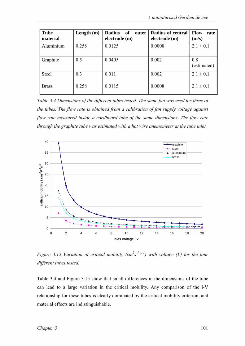
A miniaturised Gerdien device
Chapter 3 101
Tube material
Length (m) Radius of outer electrode (m)
Radius of central electrode (m)
Flow rate (m/s)
Aluminium 0.258 0.0125 0.0008 2.1 ± 0.1
Graphite 0.5 0.0405 0.002 0.8 (estimated)
Steel 0.3 0.011 0.002 2.1 ± 0.1
Brass 0.258 0.0115 0.0008 2.1 ± 0.1
Table 3.4 Dimensions of the different tubes tested. The same fan was used for three of
the tubes. The flow rate is obtained from a calibration of fan supply voltage against
flow rate measured inside a cardboard tube of the same dimensions. The flow rate
through the graphite tube was estimated with a hot wire anemometer at the tube inlet.
0
5
10
15
20
25
30
35
40
0 2 4 6 8 10 12 14 16 18 20
bias voltage / V
criti
cal m
obili
ty /
cm-2
V-1s-1
graphitesteelaluminiumbrass
Figure 3.15 Variation of critical mobility (cm2s-1V-1) with voltage (V) for the four
different tubes tested.
Table 3.4 and Figure 3.15 show that small differences in the dimensions of the tube
can lead to a large variation in the critical mobility. Any comparison of the i-V
relationship for these tubes is clearly dominated by the critical mobility criterion, and
material effects are indistinguishable.
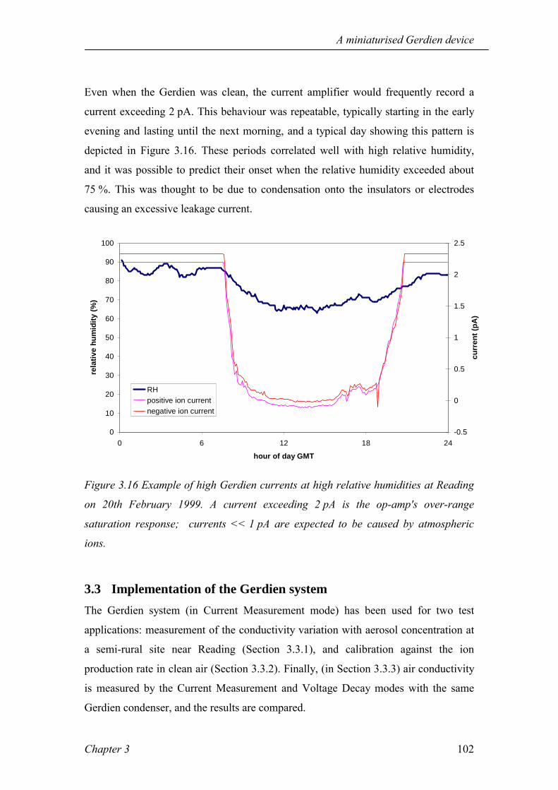
A miniaturised Gerdien device
Chapter 3 102
Even when the Gerdien was clean, the current amplifier would frequently record a
current exceeding 2 pA. This behaviour was repeatable, typically starting in the early
evening and lasting until the next morning, and a typical day showing this pattern is
depicted in Figure 3.16. These periods correlated well with high relative humidity,
and it was possible to predict their onset when the relative humidity exceeded about
75 %. This was thought to be due to condensation onto the insulators or electrodes
causing an excessive leakage current.
0
10
20
30
40
50
60
70
80
90
100
0 6 12 18 24
hour of day GMT
rela
tive
hum
idity
(%)
-0.5
0
0.5
1
1.5
2
2.5
curr
ent (
pA)
RHpositive ion currentnegative ion current
Figure 3.16 Example of high Gerdien currents at high relative humidities at Reading
on 20th February 1999. A current exceeding 2 pA is the op-amp's over-range
saturation response; currents << 1 pA are expected to be caused by atmospheric
ions.
3.3 Implementation of the Gerdien system The Gerdien system (in Current Measurement mode) has been used for two test
applications: measurement of the conductivity variation with aerosol concentration at
a semi-rural site near Reading (Section 3.3.1), and calibration against the ion
production rate in clean air (Section 3.3.2). Finally, (in Section 3.3.3) air conductivity
is measured by the Current Measurement and Voltage Decay modes with the same
Gerdien condenser, and the results are compared.

A miniaturised Gerdien device
Chapter 3 103
3.3.1 Measuring physical properties of ions with the Gerdien system In an aerosol-ion system such as the atmosphere at Reading, the concentration of
atmospheric small ions is related to aerosol concentrations, as discussed in Section
2.2.2. The values of α,β and q in Eq. 2.27 were estimated manually using a least
squares method, to minimise residuals within a sensible range. This enables the
aerosol concentration to be calculated from conductivity measurements. The aerosol
mass concentration was measured using an optical instrument, the TSI 8520
DustTrak38 and converted to a number concentration. The direct conversion of aerosol
mass to number concentration can only be an approximation, since it assumes a
monodisperse aerosol concentration of spherical particles of constant density.
0
1
2
3
4
5
6
7
0 1 2 3 4 5 6 7 8 9
Aerosol number concentration (/1011 m-3)
fS/m
negative conductivityfitted conductivity
Figure 3.17 Five minute averages of negative conductivity and aerosol number
concentration at Sonning-on-Thames, a semi-rural site NE of Reading (described in
detail by Barlow (2000)), on 12th August 1998. The fitted values are indicated in red.
The x-axis error bars are calculated from the error in the DustTrak mass
concentration measurement, converted to aerosol number concentration. Error bars
in the ordinate are ± 20%, from the error in determining the Gerdien capacitance.

A miniaturised Gerdien device
Chapter 3 104
The conductivity curve calculated from Eq. 2.27, (having fitted for α, β and q) is a
tolerable match to the measurements, but the paucity of conductivity data and its large
spread of values indicate that significant improvements to the Gerdien system were
needed. The fitted values of the coefficients were α ≈ 10-14 m3s-1, β ≈ 10-13 m3s-1, and
q ≈ 5 ion pairs cm-3s-1, which are up to two orders of magnitude away from the
textbook values of α ≈ 1.6 x 10⁻¹² m3s-1, β ≈ 1.4 x 10⁻¹² m3s-1 (Clement and Harrison,
1992) and q ≈ 10 ion pairs cm-3s-1 (Chalmers, 1967), again suggesting problematic
measurements. There may be other explanations for the difficulties encountered with
quantifying the σ-Z relationship. For example, the DustTrak is unlikely to give a true
picture of the aerosol concentration because of the approximation required to convert
mass into number concentrations, and its cutoff size (10 nm) may exclude smaller
particles participating in ion-aerosol attachment. There are also suggestions
(Dhanorkar and Kamra, 1997) that aerosol concentrations exceeding 1010 m-3, as seen
here, may invalidate the expected inverse relationship. Other experiments measuring
aerosol and conductivity (Guo et al, 1996) showed a large scatter in the fit, which
may also be expected for this case. However, these effects can not be considered until
the Gerdien data is improved.
3.3.2 Calibration in clean air A further test on the Gerdien system is to compare its readings with the source rate of
ions, which is principally from local radioactivity. The complicating effect of ion
removal by aerosol can be reduced if these measurements are made in clean air, (see
Section 2.2.3, particularly Eq. 2.20) for which reason the measurements were made at
Mace Head, W. Ireland, in summer 1999. In the recombination limit, when the aerosol
concentration is negligible, the ion concentration depends only on the square root of
the ion production rate, q, as in Eq. 2.20. Classical work (Chalmers, 1967) suggests
that alpha-radiation due to Radon isotopes measurable with a Geiger counter,
comprises a significant fraction of q at the surface.
A ZP1410 Geiger tube operated at a bias voltage of 550 ± 5 V, in the plateau of its
sensitivity curve, was located approximately 5 m away from the Gerdien condenser, at
38 This measures aerosol particles with a radius greater than 0.01µm to ± 0.001 µgm-3 or ± 1% (TSI, 1994).

A miniaturised Gerdien device
Chapter 3 105
the same height. The Gerdien system made ten samples, which were subsequently
averaged, at 0.66 Hz on a nominally three-minute cycle. Figure 3.18 shows data from
the early morning of a fine day, where the square root of the Geiger count rate is
correlated with the ion concentration, in broad accordance with theory.
0
500
1000
1500
2000
2500
6.75 7 7.25 7.5 7.75 8Hour of day (BST)
n - (c
m-3
)
0.6
0.65
0.7
0.75
0.8
G0.
5 (Bq0.
5 )
ions
Square root of Geigercounts
Figure 3.18 Negative ion concentration n- (obtained as an average of ten 0.66 Hz
samples made approximately every 3 min on 27 June 1999 at Mace Head, Ireland)
against G0.5 where the Geiger counter output rate is G. The negative ion
concentration is indicated on the left-hand axis; error bars are the standard error of
the 0.66 Hz samples. The Geiger counter output is shown on the right-hand axis,
sampled at 1 Hz and averaged every 5 minutes. The mean wind component into the
Gerdien was 5 ms-1, and the approximate aerosol mass concentration was 1 µgm-3.
The correlation coefficient is 0.38. From Aplin and Harrison (2000).
3.3.3 Measurements in both Voltage Decay and current modes Simultaneous measurements of positive and negative conductivity were made using
the two different Gerdien measurement modes for three weeks. Atmospheric air was
sampled in the laboratory using adjacent Gerdien tubes by an open window at 1.5 m

A miniaturised Gerdien device
Chapter 3 106
measuring conductivity by the two methods. A circuit (shown in Figure 3.19) was set
up to apply a voltage across the electrodes of the Gerdien condenser, turn it off and
measure the Voltage Decay as the charge on them dissipated. A manually operated
reed relay was used for the switching, and the potential was measured with a unity
gain electrometer buffer. The case of the buffer was guarded to the system ground
(the earthed screen) to minimise possible leakage paths. The buffer was connected to
a chart recorder39 to measure the change of voltage with time.
V
Centralelectrode
Guarding
Earthedscreen
Outerelectrode
1MΩ
BNC A
via BNC B
Reedrelay
12V Cell
Measuringvoltmeter
Figure 3.19 Voltage Decay measurement configuration. The 1MΩ resistor in the reed
relay part of the circuit was needed to protect from transients. The cell supplies the
bias voltage to the electrodes, controlled by the relay.
The results shown in Figure 3.19 were calculated by recording the voltage decay on a
chart recorder, calculating σ as an average from V and t values every 30 s during the
decay, which typically becomes unidentifiable after ten minutes. If the exponential
decay approximation is assumed, conductivity σ can be calculated from Eq.s 2.4 and
2.6:
39 Gould BS-272

A miniaturised Gerdien device
Chapter 3 107
tVV
oo
−=
)ln(εσ
Eq. 3.12
where V is the instantaneous measured voltage across the electrodes at a time t after
Vo was applied to charge up the electrodes. Conductivity from the current method was
calculated from Eq. 3.4.
Equal times every day were spent measuring positive and negative conductivity by the
current method, and the daily averages summed to give a total conductivity value for
comparison with measurements made by the alternative method. The daily average
values of conductivity are shown in Figure 3.20, along with the ratio of positive to
negative conductivities. This shows an average value of about 1.4, which is typical for
polluted urban air (Higazi and Chalmers, 1965; Retalis et al, 1991).
0
2
4
6
8
10
12
0 5 10 15 20 25Day in June 1998
Con
duct
ivity
(fS/
m)
0.0
0.5
1.0
1.5
2.0
2.5
+/- c
ondu
ctiv
ity
Time decay
CurrentmeasurementRatio of bipolarconductivities
Figure 3.20 A comparison of daily averages of air conductivity measured by the
Current Measurement and time decay methods (left axis). The ratio of positive to
negative conductivity is also shown (right axis). From Aplin and Harrison (2000).
Results for the air conductivity obtained from both methods are consistent, with a
positive correlation of 0.43. Experimental error in the Current Measurement method is
± 20 %, due to the error in the capacitance determination of the Gerdien condenser.
The error in the Voltage Decay method is more difficult to quantify, because the

A miniaturised Gerdien device
Chapter 3 108
validity of the exponential assumption is not known. The voltage and time values
were obtained manually from the chart recorder trace, which may contribute further
error; therefore the uncertainty is likely to be comparable to or greater than the error
in the Current Measurement results. The conductivities calculated by the two methods
agree to within the errors in the measurements, except when there is a slightly greater
discrepancy between 9 and 12 June 1998. Much of this is probably accounted for by
variations in flow speeds within the tubes, and the effects of wind direction on the
sampling orifice. Average conductivity from the Current Measurement mode was
5 fSm-1, which is in agreement with similar measurements (e.g. Blakeslee and Krider,
1992, see also Table 2.1).
3.4 Conclusions In this chapter each of the Gerdien system components has been analysed. The current
amplifier's response has been optimised for low errors due to leakage, and some
disadvantages of the original tube material were found. Investigation of leakage
currents and thermal stability show some temperature-dependent effects. The Voltage
Decay method as an alternative mode of conductivity measurement has also been
successfully deployed and results from the two methods agreed. Measurements of the
relationship between conductivity and aerosol were successful to an order of
magnitude, and calibration in clean air accords with theoretical predictions. This
suggests the techniques used can be independently validated, but their accuracy and
reliability would benefit from refinement.

A switched mobility Gerdien ion counter
Chapter 4 109
this would have obvious meteorological applications if atmospheric air were ionised to even a very small extent C.T.R. Wilson40
4 A switched mobility Gerdien ion counter In this chapter, a microcontroller is integrated with the Gerdien device described in
Chapter 3. This permits the ion counter to measure currents from ions at two different
critical mobilities. The reasoning behind this particular development strategy is
explained in Section 4.1. An overview of the computer-controlled, bimobility Gerdien
system is described in Section 4.2.
4.1 Justification and strategy One of the conclusions of Chapter 3 was that the Gerdien device can measure ions in
two modes of operation, a configuration which is clearly advantageous for self-
consistency checking. However, the tests were labour-intensive, and required manual
operation with results obtained from a chart recorder trace. Introducing some sort of
computer control would reduce these data logging difficulties, and other benefits of
such a system would greatly improve it. For example, it would be relatively easy to
switch between voltages to measure two mobilities of ion with some binary control
capability. Running the Gerdien switching in this way would also circumvent the
over-range problems, which took some hours to start. Computer control was preferred
because it would allow great flexibility in different modes of operation, for example
running the Gerdien in the voltage decay mode, carrying out basic data processing,
logging to a PC and switching between ion polarities and mobilities. A
microcontroller was chosen because of its low cost, ease of incorporation into
electronic circuits and ability to support serial communication with the PC.
4.2 The microcontrolled system The system used, pictured below in Figure 4.1 is a commercial module, the BASIC
Stamp41 based on the PIC 16C56 processor, with eight I/O pins and an integral
40 From Wilsons notebooks, referring to the cloud chamber (quoted in Galison P. (1997), Image and Logic, Chicago University Press) 41 Parallax Instruments Inc., 3805 Atherton Road, Suite 102, Rocklin, California 95765, USA

A switched mobility Gerdien ion counter
Chapter 4 110
EEPROM for program storage. Once the microcontroller is switched on, and a
program downloaded to the EEPROM via the parallel port of a PC, it runs until the
power is disconnected, and if the power is reconnected, the program will restart. This
makes it ideal for remote logging applications.
PicoammeterAnalogueto digitalconverter
Microcontroller andswitching circuitry
Reversible variablevoltage supply
PC
GERDIENIONS
Figure 4.1 Schematic showing the integrated air ion measurement system, from Aplin
and Harrison (1999)
4.2.1 Analogue to digital converter An analogue to digital converter (ADC) was necessary to convert the output voltage
from the picoammeter into a digital format suitable for serial communication. The
LTC1298 12-bit ADC (IC1 in Figure 4.2) was used in single-ended mode, controlled
by two serial lines from pins 2 and 3 of the microcontroller. A stable 2.5 V voltage
reference (measured at 2.51995 ± 0.00005V) is added to the current amplifier output
voltage before the ADC input, to ensure that bipolar ion currents can be recorded.
The level shift was tested by measuring the picoammeter output voltage accurately
with a Keithley 6512 electrometer before and after the shift stages. It was constant to
± 0.05mV for 2 < iin < +2 pA. For larger positive voltages the level shift decreases
and for smaller negative voltages the level shift increases, such that the ADC input
voltage tends to constant values of approximately +5 V or 75 mV. The computer
logging system records over range values of 4095 or 0 respectively when the ADC
receives these inputs. The ADC was calibrated by supplying it with known voltages
from a millivolt calibrator, and the output counts were serially sent to a PC; the
calibration graph is Figure 4.3 below.

A switched mobility Gerdien ion counter
Chapter 4 111
Figure 4.2 Schematic diagram of the ADC (IC1) and level-shifting circuitry, showing
the power supply and connections to the microcontroller I/O pins. From Aplin and
Harrison (2000).
y = 751.72x + 1934.9R2 = 0.9949
0
500
1000
1500
2000
2500
3000
3500
4000
-3 -2 -1 0 1 2 3
Input voltage
AD
C c
ount
s
Figure 4.3 ADC calibration, with bipolar voltages from a millivolt calibrator. The
linear response range is shown here.
4.2.2 Switching circuitry The simple switching circuit employed essentially comprised two low leakage current
relays, driven by VN10KM MOSFET transistors controlled by digital outputs from

A switched mobility Gerdien ion counter
Chapter 4 112
the microcontroller. One relay (a changeover device) was connected to two batteries
to provide positive (+9 V) and negative (-6 V) bias voltages for the Gerdien
condenser. The other relay was connected across the feedback resistor of the
picoammeter to short out the picoammeter feedback resistor. When activated, this
relay protects the picoammeter from the transients which occur immediately after the
voltage is switched.
4.2.3 Software Programs were written to control and test each component individually before the
system was tested as a whole. The program to control the ADC was from Parallax
(1998) with some modification. The separate programs controlling the ADC, serial
communication and relays were combined to make the overall control program,
GNOCLOCK, the operation of which is outlined in Table 4.1. The source code is
supplied in Appendix C.
Name Actions
Zero Turns reed relay on to protect current amplifier
Sets other relay to “0” to reduce powerconsumption
Waits for 6s
+ Turns reed relay off to allow ion currentmeasurements
Sets other relay to bias voltage 1
Waits 3 minutes
Takes 10 readings of ion current at 1Hz
Sends readings to PC via serial protocol
- Sets relay to bias voltage 2
As + above and repeats forever
Table 4.1 Outlines the actions performed by the program running on the
microcontroller. The delay of three minutes after the change of bias voltage is
required to allow complete recovery from the transient that occurs on switching.
4.2.4 Serial communication Data was sent serially to a PC at 300 baud at the following settings: no parity, eight
data bits, one stop bit, at negative polarity, and with the output mode always driven.

A switched mobility Gerdien ion counter
Chapter 4 113
There was a permanent connection from the microcontroller to the serial port of a
Toshiba 1800 laptop computer, which was mains powered and stored in a waterproof
metal box at the base of the Gerdien mast assembly. A simple data-logging program,
DATAGRAB42 was used to receive data via the serial port and store it as a text file on
the hard drive of the computer. DATAGRAB also added the time of each reading from
the PC clock (which was frequently corrected) to the file.
4.3 Results with the microcontrolled system The dual mobility microcontrolled ion counter was run at Reading University
Meteorology Field Site, with the aim of obtaining measurements of two ion size
categories, and testing the new ADC logging capability. Measurements of negative
ion concentrations at different mobilities were made by using the microcontroller
system to switch the Gerdien between two voltages of the same sign, 6 V and 9 V.
The number concentration of ions with a mobility exceeding the critical mobility,
n(µ > µc) is approximated by
( )c
c en
µσµµ => Eq. 4.1,
where e is the electronic charge and µc the critical mobility. The critical mobility was
calculated using Eq. 2.11. Flow inside the tube, which is needed to calculate critical
mobility, was determined from a fourth-order polynomial fit to the wind tunnel
measurements of flow in the tube against external ventilation (Figure 3.10). During
the measurement period, the wind component into the Gerdien tube was positive, so
the polynomial was fitted to the measurements for the case when the external wind
was aligned with the flow. The results are shown in Figure 4.4.
42 N. Ellis, Department of Meteorology, University of Reading, 1993

A switched mobility Gerdien ion counter
Chapter 4 114
0
100
200
300
400
500
600
700
800
13 14 15 16 17time of day (GMT)
ion
num
ber c
once
ntra
tion
/ cm
-3mu > 5.9 cm2V-1s-1
mu > 3.9 cm2V-1s-1
Figure 4.4 The negative ion number concentration at critical mobilities of 5.9 and 3.9
cm2V-1s-1 for the afternoon of 23rd February 1999.
4.4 Conclusions A simple microcontrolled system has been tested to measure ions by switching
between two critical mobilities and serially output the data to a PC. This is a
considerable improvement on the manual measurements described in Chapter 3, and
means the instrument can be effectively deployed for remote measurements in the
field. Encouraging results also suggest that running the instrument at more than one
critical mobility is advantageous. The success of this initial microcontrolled system
means that it can be applied to the more complex problems of controlling the voltage
decay mode and running both modes on one instrument.

The Programmable Ion Mobility Spectrometer
Chapter 5 115
To make a real, significant impact on Science, you need to invent a new instrument James Lovelock, 15th November 199943
5 The Programmable Ion Mobility Spectrometer Chapter 4 discussed an ion measuring device using an elementary switching
arrangement to select different critical mobilities. This chapter covers the
development and testing of a Programmable Ion Mobility Spectrometer (PIMS), to
permit a greater flexibility in the ion measurements. The major part is the
development of a new multimode electrometer (MME), which in addition to
measuring small currents44, can act as a voltage follower, and compensate its own
error terms in software. This allows the use of Current and Voltage Decay modes in
ion measurements. A further addition to the system described in Chapter 3 is digital-
to-analogue converter circuitry to add a range of programmable critical mobilities, by
changing the bias voltage, in the Current Mode45.
The equations used to calculate conductivity from Gerdien devices in Current and
Voltage measurement modes are:
Current Measurement method
±± =
CVi 0εσ Eq. 5.1
Voltage Decay method
σ
ετ
= 0 Eq. 5.2
for which voltage, current and time measurements are all required, which are
discussed in this chapter. I have adopted a more rigorous approach to improving and
characterising the accuracy and uncertainty in each of the quantities required in Eq.
5.1 and Eq. 5.2. Section 5.3 explains the generation of the programmable critical
mobilities by varying the bias voltage, V in Eq. 5.1. Current and voltage
measurements are discussed in the context of the two measurement modes of the 43 This quotation is paraphrased from a lecture given by James Lovelock at the Department of Meteorology, University of Reading, to a packed audience consisting almost entirely of scientists working with numerical atmospheric models. 44 In this chapter, the mode of the multimode electrometer which measures small currents will be referred to as the picoammeter mode.

The Programmable Ion Mobility Spectrometer
Chapter 5 116
multimode electrometer, in Section 5.4, which raises questions of calibration (Section
5.5). Section 5.6 discusses the two other MME modes, in which it checks its own
error terms. Section 5.7 describes the integration of the Gerdien, electronics and
microcontroller to comprise the PIMS device. Using the integrated system, the
Gerdien condenser capacitance C is measured, using a precision voltage ramp initially
developed to calibrate current measurements, and microcontroller software is
developed. Finally, in section 5.7.4, a preliminary atmospheric test compares σ
measured by the two methods. 5.1 Motivation
5.1.1 Limitations of other systems The microcontrolled Gerdien condenser system described in Chapter 3 has measured
air ion concentrations as predicted by ion-aerosol theory (e.g. Clement and Harrison,
1992), and all its components have been thoroughly tested and investigated. However,
there were clearly some aspects in need of improvement. The system was unreliable at
high relative humidities. The reason for this effect was not identified, but many
possible causes were ruled out. Aluminium as a Gerdien tube material was not
thought to be suitable for extended field measurements due to its chemical reactivity,
and the previous Gerdien design was also difficult to clean. Preliminary investigations
of leakage currents and their characteristics showed that their magnitudes and
temperature dependencies were clearly significant, but could not be tested at the same
time as the ion measurements. A further difficulty, relevant to Gerdien condenser
measurements in general, is that the instrument lacks an absolute calibration
technique. It is difficult to generate sources of ions with a well-defined spectrum and
concentration; for the concentration to be known accurately, they would have to be
confined in some defined volume, which by definition introduces problems of
unknown losses to the walls.
5.2 Objectives The primary objective is to produce a flexible instrument that can measure
atmospheric ions reliably and consistently, by further development of the
microcontrolled system described in Chapter 3. To meet the reliability criterion, there
45 The nomenclature conventions adopted in the introduction to Chapter 3 are continued here.

The Programmable Ion Mobility Spectrometer
Chapter 5 117
needs to be some way to assess the quality of the data. Direct calibration of a Gerdien-
type instrument is impractical with air ions for the reasons outlined in Section 5.1.1
above, therefore the only means of quality assurance is to include some degree of
self-calibration. This is possible with a Gerdien condenser by comparing ion
measurements made in the voltage decay and current measurement modes. Further
tests of the reliability of the data can be made by quantifying, and compensating for,
as many leakage terms as it is possible to determine. Several PIMS instruments will
be made to further improve the accuracy of the measurements.
A secondary objective of developing the programmable ion mobility spectrometer
(PIMS) is to make an instrument that is well-suited to making measurements of ionic
mobility spectra.
5.2.1 New features of the system The new system is fully automated, and controlled by the original 16C56
microcontroller, with more features added in software and hardware. It measures ions
both by either the Voltage Decay or Current Measurement techniques, allowing self-
consistency checks. A programmable range of bipolar bias voltages for spectral
measurements is attained by adding a digital bias voltage generator based on a DAC.
A current amplifier is required in the Current Measurement mode, as before.
However, voltage decay measurements require incorporation of a unity gain
electrometer follower into the signal processing system. Separate op-amps could be
used to measure voltage and current, with the inputs switched by reed relays
controlled by the microcontroller. However, this configuration would further
complicate assessing the errors due to leakage currents, which vary with the op-amp.
A new electrometer was therefore developed which uses Reed Relays to switch
between the voltage follower and picoammeter modes.
A new tube design with a stainless steel outer electrode was intended to improve the
reliability of outdoor measurements. The dimensions of the tube were chosen
specifically to measure small to intermediate ions with µ > 0.2 cm2V-1s-1 (at an
average flow rate of 2 ms-1), given the practical limitations on bias voltage supply.

The Programmable Ion Mobility Spectrometer
Chapter 5 118
This corresponds to a maximum particle radius of ~ 3 nm (Tammet, 1995), which is
approximately equivalent to the lower limit of presently-available neutral particle
detectors such as the Pollak counter (Metnieks and Pollak, 1969).

The Programmable Ion Mobility Spectrometer
Chapter 5 119
New tube design
Figure 5.1 The principal components of the PIMS Gerdien. 1 indicates the fan
position, 2 fan housing, 3 acrylic outer screen, 4 electrical outer screen (conductive
tape), 5 outer electrode, 6 central electrode, 7 central electrode BNC connector, 8
outer electrode BNC connector, 9 outer electrode rear support, 10 outer electrode
front support, 11 central electrode insulator, 12 inlet bullet-shaped cap.
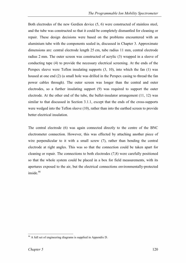
The Programmable Ion Mobility Spectrometer
Chapter 5 120
Both electrodes of the new Gerdien device (5, 6) were constructed of stainless steel,
and the tube was constructed so that it could be completely dismantled for cleaning or
repair. These design decisions were based on the problems encountered with an
aluminium tube with the components sealed in, discussed in Chapter 3. Approximate
dimensions are: central electrode length 25 cm, tube radius 11 mm, central electrode
radius 2 mm. The outer screen was constructed of acrylic (3) wrapped in a sleeve of
conducting tape (4) to provide the necessary electrical screening. At the ends of the
Perspex sleeve were Teflon insulating supports (3, 10), into which the fan (1) was
housed at one end (2) (a small hole was drilled in the Perspex casing to thread the fan
power cables through). The outer screen was longer than the central and outer
electrodes, so a further insulating support (9) was required to support the outer
electrode. At the other end of the tube, the bullet-insulator arrangement (11, 12) was
similar to that discussed in Section 3.1.1, except that the ends of the cross-supports
were wedged into the Teflon sleeve (10), rather than into the earthed screen to provide
better electrical insulation.
The central electrode (6) was again connected directly to the centre of the BNC
electrometer connection. However, this was effected by attaching another piece of
wire perpendicular to it with a small screw (7), rather than bending the central
electrode at right angles. This was so that the connection could be taken apart for
cleaning or repair. The connections to both electrodes (7,8) were carefully positioned
so that the whole system could be placed in a box for field measurements, with its
apertures exposed to the air, but the electrical connections environmentally-protected
inside.46
46 A full set of engineering diagrams is supplied in Appendix D.

The Programmable Ion Mobility Spectrometer
Chapter 5 121
Figure 5.2 Photograph of one end of the partially constructed new Gerdien tube,
before the conducting tape over the acrylic outer screen has been added. (The fan is
in place and can just be seen to the left of the fan housing).
5.3 Programmable bias voltage circuitry Bias voltages for the Gerdien's outer electrode are generated with an 8-bit digital to
analogue converter (DAC), programmable with digital signals from the
microcontroller. Since the full-scale output of the DAC is limited by its external
voltage reference Vref, which in this case is well-regulated by its 5 V power supply, an
additional high voltage op-amp (IC3 in Figure 5.3) and power supply are required to
provide the larger bias voltages necessary for the Gerdien. Power supplies limited the
bias voltage range to ± 30 V. However, since high-voltage op-amps and power
supplies capable of supplying up to 450 V or greater are available (Horowitz and Hill,
1994; Harrison, 1997b), the bias voltages could in principle be at least an order of
magnitude greater, enabling measurements of ions with µ > 0.01 cm2V-1s-1, or up to a
radius of about 16 nm.
BNC connector to central electrode (7)
Outer electrode rear support (9)
Fan housing (2)
Fan 12 V supply leads
Outer electrode (5) (inside transparent acrylic screen)
Acrylic outer screen (3)
~ 5 cm
2 cm

The Programmable Ion Mobility Spectrometer
Chapter 5 122
Figure 5.3 Schematic diagram of the bias voltage generator (from Aplin and
Harrison, 2000). PSU 1 and 2 are transformer-isolated 30 V modules (type
NMA12155) supplying non-inverting amplifier IC3 (OPA 445). A trimmable voltage
offset is applied to IC3 to allow the unipolar generation of the IC2 (MAX 550A) to
generate bipolar bias voltages.
The output voltage of the DAC IC2, V is given by
=256nVV ref Eq. 5.3

The Programmable Ion Mobility Spectrometer
Chapter 5 123
where Vref was measured as 5.061 ± 0.0005 V, and n is the voltage code supplied
serially by the microcontroller. The amplifying stage (IC3) applies a gain of 6.0 to
supply the desired bias range of ± 30 V, and an offset is also applied to its inverting
input to allow the DAC code to generate bipolar bias voltages. The DAC was
calibrated by using the microcontroller to generate a range of voltage codes47, and
measuring the voltage at the output, as shown in Figure 5.4. A least squares fit to the
data was then used to relate the DAC code to the output voltage to ± 2 %.
y = 0.224x - 27.84R2 = 0.9979
-30
-20
-10
0
10
20
30
0 50 100 150 200 250
DACCode
V
Figure 5.4 Bias voltage generator calibration, programming the DAC with the
microcontroller and measuring the output voltage. Using a least squares linear fit to
this data results in an error in the output voltage of ± 2 %, from the standard errors
in the fit.
5.4 The multimode electrometer
5.4.1 Description The multimode electrometer (MME) (Harrison and Aplin, 2000c), shown in summary
schematic form in Figure 5.6 uses five reed relays and logic circuitry to switch
between the modes of voltage follower, picoammeter, Vos check, input bias current
and electrometer leakage measurement, and charging the central electrode. An
overview of the functionality will be given here, and a complete specification is given
47 The code to initialise and control the DAC is given in Appendix C.

The Programmable Ion Mobility Spectrometer
Chapter 5 124
in Appendix A. A photograph of the multimode electrometer can be seen in Figure
5.7.
It is possible to measure the electrometer leakage current (which includes the effect of
the input bias current) and input offset voltage by grounding the non-inverting input,
as shown in Figure 5.5. In the new multimode electrometer, reed relays are used to
measure these quantities.
a) Offset voltage b) Leakage current
-+ -
+
RF
ib
Figure 5.5 Schematics for measurement of a) input offset voltage Vos b) leakage
current. (Power supplies are omitted for clarity)
A voltage reference in the electrometer circuitry, and a fifth reed relay, allows another
operating mode to charge the central electrode to a fixed potential, for subsequent
voltage decay measurements.

The Programmable Ion Mobility Spectrometer
Chapter 5 125
Figure 5.6 Functional diagram of the switching aspects of the multimode
electrometer. IC1a (LMC6042) is switched into voltage follower and current
amplifier configurations by reed relay switches RL1 to RL5 with an inverting gain
stage of IC1b added. Rf is 1012Ω. MOSFET change-over switches IC2 (4053), are
used to guard disconnected reed switch inputs, to minimise leakage. (Square pads on
the schematic are used to denote the MOSFET 'off' position and TP is a test point.)
From Harrison and Aplin (2000c).
Three input control lines are decoded by logic circuitry to drive MOSFET switches
and, where high impedance switches are required, reed relay coils labelled RL1-5 in
Figure 5.6. The reed relay drivers are also connected to LEDs so it is possible to
identify the operating mode visually. Switching on RL4 connects the signal to the
non-inverting input of the first op-amp, and puts the electrometer into the voltage
follower mode. In this mode, the outer screen needs guarding at the input to prevent
leakage. This is driven by MOSFET switch S2 in the off position and S1 in the on
position, which keeps the outer screen at the same potential as the output of IC1a. An
additional leakage-reduction feature uses the guard connection to decrease leakage at
the floating side of the open reed relays, controlled by MOSFET switches S1 and S2.
RL5 charges the central electrode to 2.0 V, via the input connection, before voltage
decay measurements can be made. In all the other measurement modes, RL5 is

The Programmable Ion Mobility Spectrometer
Chapter 5 126
necessarily off, and its open terminal is guarded at the output potential by S1 in the
off position. RL3 shorts out the feedback resistor Rf in the follower and Vos check
modes.
A further inverting, nominally x 33 gain stage, IC1b, is employed to amplify the small
signal in the Vos and (Vos + ibRf) check modes, which is activated by S3. The gain of
this stage is 1 in the measurement mode, as the combination of a high value feedback
resistor and unity gain stage has been shown in Section 3.1.3 to have the optimal
thermal stability in the picoammeter mode. Therefore, S3 in the off (measuring)
position connects a 10 kΩ resistor across IC1b, matching the resistance at the output
of IC1a so there is approximately unit gain with sign inversion.
A fifth mode charges up the central electrode to 2.0 V when RL5 is closed, with a
2.5 V REF25Z voltage reference (IC7) and a potential divider. Used in conjunction
with the bias voltage generated on the outer electrode, this can charge the electrodes
to an effective potential difference of ~ 2.5 ± 30 V for voltage decay measurements.
Figure 5.7 Photograph of the multimode electrometer.
reed relays RL1-5, air wired
Power supply and signal out
Logic in (from microcontroller)
Input connection
Screen/ guard connection
To Gerdien central electrode
PTFE insulation from case

The Programmable Ion Mobility Spectrometer
Chapter 5 127
5.4.2 Calibration of the MME Mode 1: Follower
The follower mode was calibrated by applying a voltage (± 0.05 %) from a millivolt
calibrator at the input, and measuring the voltage at the electrometer output. In this
mode, the first op-amp operates with unity gain, and the inverting second stage has a
gain close to -1. The net effect is therefore a system gain of approximately 1, which
can be derived from Figure 5.8.
y = -1.019x - 0.0006R2 = 1
-2.0
-1.5
-1.0
-0.5
0.0
0.5
1.0
1.5
2.0
-2.0 -1.5 -1.0 -0.5 0.0 0.5 1.0 1.5 2.0
V in (V)
V ou
t (V)
Figure 5.8 Calibration of the voltage follower mode, for Vin applied at the input, and
Vout measured at the electrometer output.
The additional inverting gain stage IC1b was calibrated by disconnecting it from the
preceding op-amp, and applying a signal from a millivolt calibrator directly to the
non-inverting input. The gain was -29.25 with a negligible offset, and typical
laboratory values of Vos ~ 1mV.

The Programmable Ion Mobility Spectrometer
Chapter 5 128
y = -29.252x - 0.2884R2 = 0.9968
-400
-300
-200
-100
0
100
200
300
400
-10 -8 -6 -4 -2 0 2 4 6 8 10
V in (mV)
V ou
t (m
V)
Figure 5.9 Direct calibration of the second gain stage, with Vin applied at the input to
the gain stage (with first op-amp disconnected) and Vout measured at the electrometer
output.
Mode 2: Current Amplifier
The picoammeter mode was initially calibrated as described in Section 3.2.3, by
generating a known current using a millivolt calibrator and a resistor, Rcal, which must
also be calibrated. As in Eq. 3.8, in an i-to-V converter system when there is a
secondary stage of gain G, the response includes the input offset voltage Vos
multiplied by G. So there is a compromise between using a large magnitude
calibration resistor which is difficult to measure directly, or a smaller resistor which
introduces large offsets due to magnification of Vos. In this case both approaches were
tried, and are described in Section 5.5.
5.4.3 Voltage follower mode In the voltage decay mode, the charging potential was applied directly to the central
electrode via the MME input connection. This was the simplest approach, since the
switching could then be controlled directly by the MME. Applying a potential to the
outer electrode would require modifications to both the DAC and microcontroller

The Programmable Ion Mobility Spectrometer
Chapter 5 129
circuitry, and would also be more prone to leakage (the Gerdien condenser central
electrode is designed to have ultra-low leakage).
Although the total voltage across the tube is the sum of the bias voltage and the
central electrode voltage, the follower only measures the voltage between the central
electrode and ground in a maximum range of 2.5 V. It is possible to measure the
voltage decay at either electrode because it occurs at an equal rate from both of them.
The charging potential Vf was set at + 2 V so that the voltage decay of charge was in
the optimal range to be measured. This was achieved by using a 2.5 V reference with
a potential divider. A positive electrode charging voltage was chosen because the op-
amps input bias current is much greater for negative input voltages, therefore forcing
the input voltage to be positive optimises the measurement.
Measurements in the voltage decay mode are unipolar, resulting from the voltage
followers limiting measurement range of 2.5 V to ground. If Vb = +30 V and
Vf = +2 V, then the exchange of charge due to air ions will not cause the voltage to
decay, but will increase it towards 30 V, a change which cannot be detected by the
follower. However if Vb = -30 V, adding Vf = +2 V takes the voltage across the
electrodes to above the system ground, which it will decay from to 0 V. Therefore
with a positive central electrode voltage, only negative ions can be measured.
Electrometer leakage currents are not a function of the bias voltage, therefore it is
preferable to have the highest potential difference possible across the electrodes, in
order to maximise the signal-current to leakage-current ratio.
5.5 Calibration of MME Picoammeter Mode
5.5.1 Resistive calibration techniques Rcal nominally 1GΩ
The exact value of a 1GΩ resistor constructed from 10 x (100 ± 5 %) MΩ resistors in
series was determined, by measuring the ten 100 MΩ resistors individually with the
Keithley 2000 multimeter and summing the values, to be (1.00053 ± 0.00001) GΩ.
The response of the MME picoammeter mode to currents generated with a millivolt
calibrator, and the (1.00053 ± 0.00001) GΩ resistor, is shown in Figure 5.10.

The Programmable Ion Mobility Spectrometer
Chapter 5 130
Finding the value of a 1TΩ ± 20 % calibration resistor
The (1.00053 ± 0.00001) GΩ resistor was used to calibrate another picoammeter
with Rf = 4 GΩ (Ηarrison, 1992 (henceforth H92)), which had a linear (R2 = 1)
response. The picoammeter response is known to be
[ ]GViRV osfout −−= Eq. 5.4
which can be rewritten when there is a resistive current source as
GVR
RV
GV osfcal
inout −= Eq. 5.5
Eq. 5.5 can be applied to find the value of 1TΩ ± 20 % resistor, so that it can be used
for calibration purposes. It shows that the gradient of a calibration graph of the
picoammeter output voltage Vout, against the voltage used to generate a current with
the calibration resistor Rcal gives (G.Rf /Rcal). As the gain can be calculated from the
offset of Eq. 5.5, if one of the resistance values in Eq. 5.5 is well-known, then the
gradient of Eq. 5.5 can be used to find the other resistance. This method was applied
to measure the 1TΩ ± 20 % resistor, by using it as the current-generating resistor Rcal
with the Η92 picoammeter which has Rf = 4 GΩ . The value of the resistor was
deduced to be (0.7720 ± 0.0004) TΩ.
Rcal nominally 1TΩ
The response of the MME in picoammeter mode to currents generated with a millivolt
calibrator using the (0.772 ± 0.0004) TΩ and (1.00053 ± 0.00001) GΩ resistors, was
then measured. The results are shown in Figure 5.10.

The Programmable Ion Mobility Spectrometer
Chapter 5 131
y = 0.8952x + 0.0321R2 = 0.9991
y = 0.9297x - 0.7671R2 = 0.9949
-3.0
-2.0
-1.0
0.0
1.0
2.0
3.0
-3 -2 -1 0 1 2 3
i in (pA)
Vout(V)
772G1.0053GLinear (772G)Linear (1.0053G)
Figure 5.10 Resistive calibration of the MME in picoammeter mode, using calibration
resistors of 772 GΩ and 1 GΩ. The error bars on the abscissa result from the
uncertainty in the magnitude of the calibration resistor.
In Figure 5.10 some inconsistencies can be seen between the two calibration methods.
Calibration with Rcal = 1.00053 GΩ has a significant offset of -750 mV, in contrast
with Rcal = 772 GΩ when the offset was only 3 mV. However, the
Rcal = 772 GΩ calibration was inconsistent with time, and the gain varied by 7 %
when the same instrument, which had not been used in the meantime, was recalibrated
9 days later. In Appendix B the system response is derived, and the analysis suggests
that significant offsets can result from amplification of the input offset voltage when
Rf >> Rcal. This hypothesis was tested by estimating the magnified offset. Vos was
measured with the MME in mode 3 (Table A.1), and found to be ~ 1 mV. It is clear
that since Vos ~ 1 mV, this multiplied by a gain equivalent to Rf /Rcal. accounts for
almost all of the offset in the calibration. It can be concluded that it is unsatisfactory
to use 1 GΩ calibration resistors in conjunction with much larger feedback resistors,
because the multiplied input voltage offset changes with temperature, and over time,
are sufficient to degrade the calibration. This is explicitly given in the overall system
response, which is shown in Appendix B as:

The Programmable Ion Mobility Spectrometer
Chapter 5 132
( )[ ]
++++−=
cal
fosfLbout R
RVRiiiGV 1 Eq. 5.6
The term showing the sum of input, bias ib and leakage currents iL in Eq. 5.6 explains
the unsatisfactory temporal variation of the gain when the 772 GΩ calibration resistor
was used. As explained in Appendix B, both the gain and intercept of the Vout-i
calibration graph will only remain constant if the input bias current, electrometer
leakage currents and input offset voltage are invariant, which is unlikely. In
conclusion, the method described of resistive calibration described above is inherently
unsuitable for picoammeter calibration, because of amplification of the offset voltage
and changes in leakage currents.
5.5.2 A capacitative calibration technique: the femtoampere current reference In response to the problems with resistive calibration explained in Section 5.5.1, a
different calibration technique was developed based on a capacitative principle, which
ensures Rcal is large (Harrison and Aplin, 2000a)48. It generates a slowly varying
voltage ramp (± 52.5 mVs-1, over 32 s) using a crystal oscillator. If this signal is
presented to a 10 pF polystyrene capacitor, it produces a bipolar current of order
± 500 fA, with its sign depending whether the voltage ramp is on the rising or falling
edge. For the calibrator used in this Thesis, the current was measured with the
Keithley 6512 electrometer to be ± 470 ± 2 fA over the temperature range -22 to
21.7 ºC, and was also temporally stable. The femtoampere current reference was used
to calibrate the MME picoammeter mode, which is shown in Figure 5.11.
48 The principles of the capacitative calibrator (Harrison and Aplin, 2000a), are described in Appendix B.

The Programmable Ion Mobility Spectrometer
Chapter 5 133
y = 1.1039x + 0.0231
-0.6
-0.4
-0.2
0
0.2
0.4
0.6
-0.6 -0.4 -0.2 0 0.2 0.4 0.6
i in (pA)
V ou
t
Figure 5.11 MME calibration in picoammeter mode, with currents generated from the
precision voltage ramp connected to a 10 pF capacitor. The offset was measured
when the picoammeter input was connected to the screened 10 pF capacitor, with the
ramp generator disconnected. The picoammeter gain is (1.104 ± 0.004) V/pA, and the
offset is (2.3± 0.1) mV (errors are the standard error in the least squares linear fit).
5.6 Testing of MME measurement modes
5.6.1 Error term modes The input offset voltage was measured at the Reading University Meteorology Field
Site on eight days. Vos was observed to vary slowly with time, so the averages for
each day of measurements were calculated and compared against the average
temperature over the same period in Figure 5.12.

The Programmable Ion Mobility Spectrometer
Chapter 5 134
y = 0.0093x + 2.3685R2 = 0.9131
2.45
2.50
2.55
2.60
0 5 10 15 20 25mean temp (deg C)
mea
n of
fset
vol
tage
Vos
(mV)
Figure 5.12 Variation of mean input offset voltage of the MME with mean
temperature, over eight diurnal cycles.
Figure 5.12 shows that Vos varies linearly with temperature at a rate of 9.3 µVºC-1, and
Vos typically varies in the range 1-10 µVºC-1, (Peyton and Walsh, 1993) with 10 µVºC-
1 quoted by the manufacturers as typical for the LMC 6042 op-amp used in the MME.
The errors introduced due to this source are negligible relative to the ion current,
because after calibration the effect of Vos included in the picoammeter mode output
voltage only represents currents of order atoamperes.
The leakage term iL, found directly using electrometer modes 3 and 4, is composed of
the input bias current plus some leakage currents within the MME. The likely origin
of the measured leakage currents can be assessed from considering which relays
contribute to the leakage in each mode. In mode 4 (leakage current test), RL1, RL3,
RL4 and RL5 are open. RL5 is guarded, and RL4 has no current path, so their
contributions can be neglected and the leakage must be from RL1, RL3 or leakage
across the screen to the input. In mode 3 (current measurement) a similar argument
suggests that the leakage current is primarily from RL3 or the screen. This shows that
the leakage currents in each mode are slightly different, because the nature of any
self-monitoring instrument necessarily requires its configuration to change to measure

The Programmable Ion Mobility Spectrometer
Chapter 5 135
signal and leakage. Though it appears valid to compensate for some of the errors by
this method of switching between modes, it is ultimately unable to completely correct
for all electrometer leakages. However, the results of laboratory tests shown in Figure
5.13 imply substantial compensation for the leakage current measured in MME mode
2 is relevant, since iL was strongly temperature dependent, with a variation of -
9 fΑºC-1. At a bias voltage of 20 V, this would contribute an error of 0.4 fSm-1ºC-1 to
the conductivity measurement, which is a significant drift.
15
16
17
18
19
20
21
32.8 33.3 33.8 34.3day of year
labo
rato
ry te
mpe
ratu
re (d
eg C
)
-90
-85
-80
-75
-70
-65
-60
-55
-50
leak
age
curr
ent (
fA)
Temperatureleakage current
Figure 5.13 Diurnal cycle of laboratory temperature measured with a platinum
resistance thermometer (Harrison and Pedder, 2000) and MME leakage current,
found using modes 3 and 4, which is plotted on the right hand axis.
5.6.2 Compensating for leakage currents in the ion current measurement To justify compensating the ion current measurements for the leakages measured in
mode 2, it must be shown that the leakage currents are small with respect to the ion
currents, and that they vary more slowly than they are sampled. The time series of i/iL,
which shows the relative magnitudes of leakage and signal, was constant with a well-
defined mean up to timescales of about two hours, but there was a slow drift, due to
the temperature dependence of iL. Over a whole day, a linear fit of i against iL had
R2 = 0.41. This suggests that neither i nor iL is fluctuating fast enough to reduce the
effectiveness of the compensation procedure. Short-term fluctuations in iL may

The Programmable Ion Mobility Spectrometer
Chapter 5 136
introduce some uncertainty into the current measurement, because they are both 10 s
(1 Hz) averages made with a 5 s pause between them. If iL is fluctuating rapidly, then
subtracting its average value may not be an adequate compensation. iL was measured
in the laboratory at 1Hz for half an hour and the mean 30 s standard deviation was
calculated, which is the same time-scale as the compensation. It was 0.5 %, which is
comparable to the error in the electrometer calibration.
0.50
0.52
0.54
0.56
0.58
0.60
0.62
0.64
0.66
0.68
0.70
39.6 39.7 39.8 39.9 40 40.1 40.2 40.3 40.4 40.5year day (GMT)
mea
sure
d cu
rren
t (pA
)
30
35
40
45
50
55
60
65
70
75
80
85
90
leak
age
curr
ent (
fA)
ii - leakageleakage
Figure 5.14 Comparison of measured im (thin trace), leakage iL (thick trace) and (im
iL) currents sampled every minute for 18 hours in the laboratory, in response to a
resistively generated current of ∼ 600 fA. iL is shown in the blue (dotted) trace on the
right-hand axis.
Figure 5.14 shows that the leakage current is at most 8 % of the total signal, and
subtracting it from the measured current brings the mean closer to the reference
signal. Here, the reference signal was generated using a 1 TΩ resistor, and is therefore
also subject to temperature fluctuations, but since identical calibration and feedback
resistors were used for all the current measurements, they could be expected to track
together in the same thermal environment. (An absolute calibration technique has
been described in Section 5.5.2). The electrometer leakage current can be seen as a
source of slowly varying offset, shifting the average value of the signal. When it is
compensated for, the average moves but the short-term fluctuations in the signal are

The Programmable Ion Mobility Spectrometer
Chapter 5 137
diminished. In further data analysis, the iL contribution has been subtracted from the
ion current measurements, as a correction to the mean.
5.6.3 Switching transients In Section 3.1.4 it was shown that one reed relay injects typically 6 fC of charge into
the system when closed. It is necessary to allow some time for the system to recover
from each transient, so that it does not affect the measurements. However, the
comparisons between measurements made in different MME modes, such as the
subtraction of Vos measured in mode 3 from the results in mode 4 to calculate
electrometer leakage currents, necessitate making the measurements as immediately
consecutive as possible. The optimal recovery time is the time it takes for the
exponential decay from the transient to become indistinguishable from the real signal.
An empirical investigation to find the optimal recovery time was carried out, by
making measurements with the tube sealed but with the voltage switching on, and
varying the time before starting to measure after the voltage was changed. This was
determined by using the microcontrolled system to start logging with 2 Hz samples
immediately after the voltage was switched, and also with a pause before the start of
logging. The time series were then examined to see if the samples showed decay
characteristics, by fitting a straight line to each set of voltage and time samples and
calculating the gradient. If the mean gradient of all the voltage time series was
negative, this was used as an indicator that the decay from the transient was
continuing to dominate the signal. Recovery times from 0-30 s were tested, and 10 s
was the shortest settling time after which the decay from the transient had finished.
Hence, 10 s was the recovery time chosen for use in the control program between
mode changes.
5.6.4 Electrometer control software Dedicated microcontroller programs were developed for controlling and testing each
electrometer mode separately. Source code is given in Appendix C, and Table 5.1
below summarises the function of each program.

The Programmable Ion Mobility Spectrometer
Chapter 5 138
Program
Name
Function
ICAL Picoammeter (mode 4) calibrator with the femtoampere current
source
DECAY Charges up central electrode to 2.5 V and logs decay in follower
mode (mode 1) at 2 Hz.
IBLOG Alternates between modes 3 and 4 and logs them, with a
header so they can be separated.
Table 5.1 Descriptions of the three programs used to test the MME modes
independently.
5.7 Integrated PIMS system This section describes the integration of the separate components into a complete
PIMS system. The capacitance of the Gerdien condenser is determined using the
femtoampere reference (Harrison and Aplin, 2000a), and the overall control program
is described. Three of these PIMS systems were constructed, and some results from
them will be compared in Section 5.7.4.
5.7.1 Measurement of capacitance of Gerdien condenser Since the femtoampere reference (Harrison and Aplin, 2000a) generates a current by
passing a voltage ramp through a capacitor, using precision components, it is clear
that, alternatively, if the current from a capacitor connected to the voltage ramp is
measured accurately, its capacitance can be determined. This technique was employed
to calculate the capacitance of the Gerdien condenser, which has classically not been
known accurately, as explained in Chapter 2. In the miniature Gerdien condenser
there is also a finite capacitance CS between the outer electrode and screen. This is in
addition to the exposed capacitance (Arathoon, 1991), which is the effective
capacitance of the Gerdien exposed to ions, and is required for conductivity
calculation from Current Mode results (Eq. 2.17). Here the exposed capacitance is
referred to as CG, between the outer and central electrodes, which determines the ionic
charge stored on the electrodes. These capacitances, which are unavoidably present in
series, are schematically represented in Figure 5.15.

The Programmable Ion Mobility Spectrometer
Chapter 5 139
Central electrode
Outer electrode
Screen
CG
Cs
Figure 5.15 Schematic of the capacitances between the Gerdien condenser electrodes
and screen.
The capacitance CS is clearly not associated with ion measurements made with the
Gerdien condenser, since they only involve a flow of charge to or from the central
electrode. It must therefore be discounted in any measurement of capacitance. This
was achieved by shorting the outer electrode to the screen, as shown below in Figure
5.16, so CS cannot contribute to the current measured.
RAMP VOLTAGEGENERATOR
FEMTOAMMETER
C
CS
Outer electrode
Inner electrode
Screen
Figure 5.16 Schematic of the circuit used to measure the Gerdien capacitance.
The mean magnitude of current, measured with the Keithley 6512 electrometer, was
476 ± 1.5 fA (standard error of 6 cycles, 12 current measurements). Hence,

The Programmable Ion Mobility Spectrometer
Chapter 5 140
CG = 9.07 pF, and the standard error of the current above is 0.3 %. Stray capacitance,
for example from the connections probably dominates the errors in the capacitance
determination; therefore the error in the Gerdien condenser capacitance is estimated
as 1 %, 0.09 pF for this Gerdien. This approach has reduced the uncertainty in the
current method of conductivity measurement due to the capacitance term by an order
of magnitude, compared to other capacitance determination methods, e.g. Aplin and
Harrison (1999), Smith (1953).
5.7.2 Complete control program The individual control programs for calibration of individual components described
above (Section 5.6.4) were merged with the ADC control program described in
Chapter 4 to control the whole system. As a variety of measurements were being
made, a more sophisticated logging strategy was needed. The sampling rate is a
compromise between taking enough samples to average and smooth high-frequency
fluctuations, and rapid sampling to improve the voltage decay and current
measurement intercomparisons. In the voltage decay mode, the ion current flowing is
inferred from the rate of change of potential. Hence, time averaging is not relevant in
this case, and the samples should be temporally close to maintain consistency of
atmospheric conditions during the sampling period. Therefore, ten measurements of
the voltage across the tube were made at 2 Hz.
The sampling characteristics for the other three MME modes were chosen to minimise
the standard deviation of the raw measurements, before averaging. This was tested by
calculating the variability of measurements at different frequencies, and for varying
periods, from a sealed Gerdien in the laboratory at zero bias voltage. Under these
conditions, the only variability in the ion concentration should result from background
ionisation, therefore the measurements made can be considered equivalent to a
background noise level. The minimum variability in the background noise level was
found when ten measurements were made at 2 Hz, and these settings were empirically
selected for application in the final control program.

The Programmable Ion Mobility Spectrometer
Chapter 5 141
The final control program was called MMESYS*49, where * represents the PIMS
number it was written for50. Calibrations of the components differed slightly, and in
order to ensure the same ionic mobilities were measured from instrument to
instrument, slightly different variables (and timings, discussed in Section 5.7.3) in the
programs were required. As well as controlling the different mode switching,
MMESYS averages (except in the follower mode) and logs data and sends it serially
to the PC. This format was chosen to ease the compensation procedure and separation
of results from the Current Measurement and Voltage Decay modes, when the text
files are subsequently calibrated using MS Excel. A sample set of lines from the PC
data file is shown below, and is explained in Table 5.2.
YearDay, Time, I, DACcode1, (ib+Vos), Vos, i
YearDay, Time, V, DACcode1, V1…Vn
YearDay, Time, I, DACcode2, (ib+Vos), Vos, i
YearDay, Time, V, DACcode2, V1…Vn
…
YearDay, Time, I, DACcodeN, (ib+Vos), Vos, i
YearDay, Time, V, DACcodeN, V1…Vn
YearDay, Time, I, DACcode1, (ib+Vos), Vos, i
YearDay, Time, V, DACcode1, V1…Vn
49 Source code is in Appendix C. 50 Use of the name MMESYS indicates general properties of the program are under discussion. MMESYS* is used to indicated the aspects in which the individual PIMS programs were different.

The Programmable Ion Mobility Spectrometer
Chapter 5 142
Quantity Description
Yearday Day of year, from the PC clock (0-366)
Time Time from the PC clock, hhmmss (0-235959)
I or V V denotes voltage decay mode, I denotes current measurement/ error
check mode
DACcode DAC code to represent bias voltage, where there are N in total ( where
N ≤ ~15, limited by the microcontroller memory)
ibRf+Vos Output in ADC counts, 10s average (0-4095)
Vos Output in ADC counts, 10 s average (0-4095)
i Output in ADC counts (picoammeter mode), 10 s average (0-4095)
V1…Vn n voltage decay measurements, where n = 10 in MMESYS
Table 5.2 Format of the serial output logged by the PC.
5.7.3 Timing and Synchronisation The time of the measurement is derived from the PC clock, which is frequently set
manually on the laptops used, at the beginning of each line of logged data. The
electrometer leakages and offsets are subsequently subtracted from the current
measurement51, and therefore the three 10 s averages are effectively assumed to be
simultaneous with an observation. Section 5.6.2 explains that the ratio of the leakage
current to the measured current remains constant for timescales much greater than
this.
In the PBASIC microcontroller programming language, timing is controlled by the
PAUSE milliseconds command, where milliseconds is the pause time
expressed in milliseconds ± 1 %. Parallax (1998) explain that the microcontroller
BASIC interpreter takes at least 1 ms longer than the PAUSE instruction to carry out
programming loops including this command. Since the PIMS control programs
typically include several such loops, errors are expected in the timing, which were
observed when using the microcontrolled picoammeter with the voltage ramp derived
current source. This has a precisely-timed ramp time of 32 s (Harrison and Aplin,
2000a), and when trying to make the microcontroller program match this cycle, there
was a 15 % error. Processing the voltage decay data involves least squares fitting to

The Programmable Ion Mobility Spectrometer
Chapter 5 143
voltage as a function of time, and therefore the internal timing of these measurements
does need to be known accurately. The voltage decay sampling frequency was
nominally 2 Hz, but was measured to be a constant 1.98 Hz with a digital stop clock,
on which the timings for data processing were based. (The error in the
microcontrollers internal clock was insignificant on the 5 s timescale). The
inconsistency between different devices was also investigated.
Three PIMS systems were constructed, and inconsistencies between the
microcontrollers internal clocks meant that the measurements were asynchronous,
even when the same program was running on them all. Test programs indicated that
the internal timers were tuned slightly differently, so that the PAUSE command
produced a pause of a length which was a constant factor different from the same
command executed on a different microcontroller. The recovery time between
switching the bias voltage was therefore lengthened slightly by an empirically
determined factor in the PAUSE statement in MMESYS*, so that all the
microcontrollers had the same program time period. Operating the three
microcontrollers from one switchable power supply allowed all the programs to be
started simultaneously.
5.7.4 Testing the integrated PIMS systems An important test of the integrated Gerdien system is to compare results from the two
ion measurement modes of the MME. The complete system was run at the Reading
Meteorology Field Site on 22nd March 2000. For running in atmospheric air, the
PIMSs were housed in watertight plastic boxes (28 x 18 x 8 cm), as shown in Figure
5.17. The Gerdien inlets protruded, and the microcontroller/ADC, MME and
DAC/power supply circuitry were in three small metal boxes, wired inside the plastic
box. There were two Buccaneer connectors on the plastic box, one two-way for power
from a 12 V lead-acid battery, and one six-way carrying serial and parallel
connections to a laptop PC for logging and programming respectively.
51 Data processing will be discussed in detail in Chapter 6.

The Programmable Ion Mobility Spectrometer
Chapter 5
Figure 5.17 Photograph of the PIMS ready for
on box).
First, PIMS no. 3 was run for approximately
both current and voltage modes. After PIMS no
completely different system, was run for a
Meteorological conditions remained effectively
Conductivity was calculated from the standard e
τ calculated from a Microsoft Excel exponential
of current used in Eq. 2.17 was (i-iL).
52 The details of data processing will be discussed in Chap
fan
DAC/ Bias voltage supply
MME
Connection to central electrode
Connection to outer electrode
To PC serial and parallel ports
To 12 V power supply
ADC/ Microcontroller
28 cm
inlet
18 cm
144
atmospheric deployment (without lid
two hours measuring conductivity in
. 3 was disconnected, PIMS no. 2, a
short time at the same location.
constant throughout the test period.
xpressions Eq. 2.17 and Eq. 2.4 with
fit to the voltage decays52. The value
ter 6.

The Programmable Ion Mobility Spectrometer
Chapter 5 145
0
20
40
60
80
100
14.5 15 15.5 16 16.5
hour of day (GMT)
nega
tive
cond
uctiv
ity /
fS/m
System 3, current methodSystem 3, decay methodSystem 2, current methodSystem 2, decay method
Figure 5.18 Comparison of negative conductivity calculated with results from both
methods, and with PIMS 2 and 3 at Reading on 22nd March 2000.
There is a general agreement between the conductivity calculated by the two methods,
although the absolute magnitudes do vary. PIMS 2 shows comparable mean values.
Further analysis is required to explain the disparities in the measurements, but it is
clear that the different instruments and techniques show comparable behaviour. All
the major peaks are detected by both measurement modes, and the mean value is
about 12 fSm-1, which conforms to typical fair weather measurements in urban
locations (e.g. Chalmers, 1967; previous measurements are discussed in Chapter 2).
5.8 Conclusions A programmable ion mobility spectrometer has been designed and tested in this
chapter, incorporating a new multimode electrometer and improved Gerdien design.
The errors in previous conductivity measurements will have been significantly
reduced by determination of the Gerdien capacitance to 1 %, and compensation for
temperature-dependent voltage offsets and some leakages. A further innovative
feature is the ability to check self-consistency from both current and voltage

The Programmable Ion Mobility Spectrometer
Chapter 5 146
measurements, results have agreed from two separate PIMS instruments, and such
self-calibration of the device appears feasible.

PIMS atmospheric calibration and testing
Chapter 6 147
when all conventional physics failed, some property of aerosol could always be invoked to get out of a difficulty, but whether these were cosmetic, or physical in origin is difficult to judge John Green53
6 PIMS atmospheric calibration and testing In this chapter, the testing of the PIMS instrument in the atmosphere is described in
detail. The deployment of three individual PIMS, each with two ion measurement
modes, facilitates self-calibration, and these results are discussed in sections 6.4 and
6.5. The PIMS results are also compared to measurements from two independent
external instruments, a Geiger counter, which responds to ionising radiation, (Section
6.3) and another Gerdien ion counter of more classical design (section 6.6.1). This
chapter also necessarily contains, as a precursor to the results, details of the
experimental configuration and data processing, which are outlined in Sections 6.1
and 6.2.
The structure of the calibration and comparison procedures is explained graphically in
Figure 6.1. Three PIMS instruments were constructed, and the simplest test is of
internal consistency between the two modes on each instrument. The results from
each mode can then be compared to other PIMS measurements. The most rigorous
calibration procedure is to compare the PIMS results to other instruments measuring
ions, a Geiger counter and a Gerdien condenser.
53 Green J. (1999), Atmospheric Dynamics, CUP

PIMS atmospheric calibration and testing
Chapter 6 148
Currentmeasurement
Voltage decay
PIMS 1
Self-consistencychecking between twomeasurement modes-section 6.4
Calibrationagainstindependent ionmeasurements –section 6.6.1
ExternallyconstructedGerdien
Currentmeasurement
Voltage decay
Further self-consistency checkswith three PIMSs–section 6.5
Comparison withion productionrate – section 6.3
Geigercounter
Currentmeasurement
Voltage decay
PIMS 2
PIMS 3
Figure 6.1 Block diagram showing the approaches to PIMS consistency.

PIMS atmospheric calibration and testing
Chapter 6 149
6.1 Description of PIMS atmospheric deployment Measurements were made at Reading University Meteorology Field Site with the
three PIMS instruments mounted next to each other, with the inlets facing south, on a
mast at 1.25 m. A photograph of the mast is shown in Figure 6.2. This was the same
height the Geiger counter had been at for previous long-term monitoring of local
radioactivity at the Field Site. For effective comparison with the Geiger count rate, the
PIMS needed to be mounted at the same height. The orientation was chosen so that
the average wind velocity would be as close as possible to the wind tunnel test speed
of 2 ms-1, for which the bias voltage range was selected. (Mean wind speed at the site
for 1999 was 2.2 ms-1, and direction 197º, so the southerly component is 2.1 ms-1,
which matches the fans ventilation rate almost exactly). The inlets were arranged as
close as possible, but the plastic PIMS housing kept the minimum separation to about
15 cm; this can be seen in Figure 6.3.
ThreePIMSs(inlets facingthe camera)
12V lead-acid battery
Geiger counter(Geiger-Muellertube windowfacing down)
Metal casefor threelogginglaptop PCs
Buccaneerconnectors toPC and battery
Figure 6.2 Photograph of the PIMSs running at Reading University Meteorology
Field Site.

PIMS atmospheric calibration and testing
Chapter 6 150
20 cm
5 cm
Wing-nutsattach thePIMS to themast arm
12V DCconnector tolead-acidbattery
Six-wayconnector toPC serial andparallel ports(behind 12 Vconnector)
PIMS inlets
Figure 6.3 Close-up photograph, taken from the south, showing the PIMS inlets and
connections.
6.2 Calibration of raw data Data is stored in a text file by the logging PC as integer values (ADC counts) from 0
to 4095, representing an output range of ± 2.5 V. Voltage calibration of the ADC
converter was described in section 4.2.1; further calibration is then required,
depending on the MME mode, to convert the voltage into the correct magnitude of ion
current or electrode voltage. The details of this procedure for the two ion
measurement modes, and the calculations performed to obtain conductivity values
from the measurements, are described below.
6.2.1 Current Measurement method In this mode the measured current imeas is calculated by calibrating the ADC output, as
shown in the schematic diagram (Figure 6.4). A voltage offset of 2.5 V has to be
added to the bipolar current measurement because the ADC is only unipolar, (see
section 4.2.1), therefore 2.5 V must be subtracted from the voltage obtained from the
ADC counts before the MME picoammeter calibration can be applied. The
electrometer leakage current iL is calculated separately from the results of the two

PIMS atmospheric calibration and testing
Chapter 6 151
error checking modes, and is subtracted from imeas to give the compensated current, ic
which is used to calculate conductivity in the conventional manner,
CV
icoεσ = Eq. 6.1
for bias voltages V set by the DAC. In Figure 6.4, the entire calibration and
compensation procedure is summarised. It begins with the current and error check
mode measurements in the integer ADC format stored in the PC text file, and follows
the process through to the corrected current used to calculate conductivity ic.

PIMS atmospheric calibration and testing
Chapter 6 152
ADC Counts
(Currentmode voltageoutput) +2.5V
Vos modevoltageoutput
(Vos + iLRf)mode voltageoutput
Current modevoltageoutput
Input offsetvoltage Vos
Leakagecurrent IL
-2.5VVos modecalibration:section 5.4.2
-Vos÷Rf
Picoammetermodecalibration:section 5.5
Measuredcurrent imeas
Leakagecompensatedcurrent ic
-iL
Figure 6.4 Schematic showing the calibration and correction procedures required to
obtain a compensated current measurement. The three modes operate sequentially,
for 10 s each. This procedure is repeated for measurements at each bias voltage.

PIMS atmospheric calibration and testing
Chapter 6 153
6.2.2 Voltage Decay method In this mode, repeated electrode voltage measurements are required. Figure 6.5 below
outlines the procedure used to calculate the voltage between the Gerdien condensers
central and outer electrodes. Since there is a bias on both electrodes, the potential
difference the ions are subject to in the Gerdien is determined by the sum of the bias
voltage Vb (potential difference between outer electrode and ground) and Vf, the
voltage measured by the MME at the central electrode with respect to ground. This
will be referred to here as Vdecay,, where Vf is a function of time.
)()( tVVtV fbdecay += Eq. 6.2.
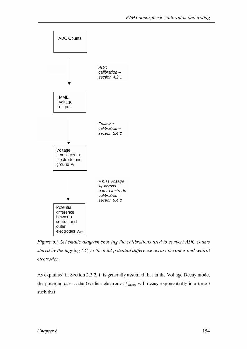
PIMS atmospheric calibration and testing
Chapter 6 154
ADC Counts
Potentialdifferencebetweencentral andouterelectrodes Vdec
ADCcalibration –section 4.2.1
Followercalibration –section 5.4.2
Voltageacross centralelectrode andground Vf
+ bias voltageVb acrossouter electrodecalibration –section 5.4.2
MMEvoltageoutput
Figure 6.5 Schematic diagram showing the calibrations used to convert ADC counts
stored by the logging PC, to the total potential difference across the outer and central
electrodes.
As explained in Section 2.2.2, it is generally assumed that in the Voltage Decay mode,
the potential across the Gerdien electrodes Vdecay will decay exponentially in a time t
such that

PIMS atmospheric calibration and testing
Chapter 6 155
−=τ
tVtVdecay exp)( 0 Eq. 6.3.
Taking logs, this can be rearranged to give
0lnln VtVdecay +−=
τ Eq. 6.4,
and recalling that
τεσ o= Eq. 6.5,
it is clear that the gradient of a graph of ln Vdecay against time is equivalent to -σ/ε0.
This approach was applied to calculate conductivity from the time series of Vdecay. The
time of each voltage reading with respect to the start of the measurement (when the
reed relay which activates the charging of the central electrode is switched off) is
approximately determined using the microcontroller program, and was also calibrated
using a digital stopwatch (see section 5.7.3). Since only negative ions can be
measured at the central electrode during the active decay from 32.5 V to 30V (see
section 5.4.3), all results here refer to negative ion measurements. An MS Excel least
squares linear fitting worksheet function, LINEST, was then applied to the natural
logarithm of the magnitude of each voltage reading, with time as the abscissa, starting
from a first sample at t = 0.505 s.
LINEST was also used to calculate the standard error in fitting the gradient to the
points, which can be used to calculate an error in σ resulting directly from the least
squares regression procedure. The coefficient of determination54 R2, was also
determined using the same function. This is a goodness of fit parameter from 0 to 1.
If R2 = 1, there is no difference between the y-values predicted by the theory and the
actual y-value, and decreasing R2 indicates increasing inappropriateness of fitting the
regression equation to the data (Johnson and Bhattacharrya, 1996). The fitting
procedure described above resulted in a mean R2 = 0.65, which was similar for all the
data sets. To test whether this fraction of exponential decays could occur by chance, a
Monte Carlo simulation was run to generate 1000 random voltage decay traces. This

PIMS atmospheric calibration and testing
Chapter 6 156
simulates the input that would be generated by noise. The same exponential curve
fitting procedure was applied to the randomly generated decays. Only 0.15 % of the
random decay data had R2 > 0.65, which strongly suggests that only a tiny fraction of
the exponential decays seen here could occur by chance. For exponential fitting to voltage decay data, the coefficient of determination is a
useful quantity, because, as suggested in Section 2.2.2, an exponential decay may not
always be an appropriate method to calculate conductivity. The critical mobility
(minimum mobility) of ions contributing to the measurement decreases as the voltage
decays, and therefore the number of ions actually being measured varies with decay
voltage. This is equivalent to the charge on a capacitor decaying across a variable
resistor; thus the theory outlined in Section 2.2.2 leading to Eq. 6.4, may not apply in
some cases. The effectiveness of assuming an exponential decay depends on the
characteristics of the ion mobility spectrum, which provides information about the
number of ions having each mobility55. For these reasons, the standard error of the
exponential fit is not equivalent to the error in the measurement. If the critical
mobility were invariant with voltage, there should always be an ideal exponential
decay and in this limit, the standard error of the fit would be the true error. The
standard error of the exponential fit may therefore be considered as a worst case
estimate of the measurement error.
The raw data does not always follow an approximately exponential decay, in some
cases the voltage across the electrodes increases, and over the 5 s of sampling the
voltage can fluctuate considerably. A sample set of voltage decay time series,
measured over one hour from 12:25 to 13:25 on 27 June 2000 is shown below in
Figure 6.6. The decay characteristics show substantial variation over this relatively
short time, which is common to all the voltage decay measurements. The best and
worst exponential fit lines in the hour of measurements are also shown, and span
R2 = 0.88 to 0.19. If the voltage across the electrodes increases anomalously, the
54 MS Excel defines R2 as the square of the Pearson product moment correlation coefficient, r, a dimensionless index that ranges from -1.0 to 1.0 inclusive and reflects the extent of a linear relationship
between two data sets.( ) ( )( )
( ) ( )[ ][ ]
−−
−=
2222 YYnXXn
YXXYnr
55 Effects of the ion spectrum on voltage decay data will be discussed in more detail in Chapter 8.

PIMS atmospheric calibration and testing
Chapter 6 157
gradient will be a positive number and the calculated conductivity will be negative. It
is consequently inferred that the electrodes are charging up, and the data is rejected. In
Figure 6.6, some data sets show both decay and charging characteristics, for example
at 12:41 there is an exponential decay for the first three seconds which then changes
direction. If an exponential is fitted to the part of the data which is showing decay
characteristics, then it has an R2 value of 0.86, but a fit to the whole time series has
R2 = 0.50. This will also affect the magnitude of the calculated conductivity, which
increases as the gradient of the exponential curve decreases.

PIMS atmospheric calibration and testing
Chapter 6 158
y = 22.30e0.00x
R2 = 0.00
y = 22.3075e-0.0025x
R2 = 0.8398
21.95
22.00
22.05
22.10
22.15
22.20
22.25
22.30
22.35
0 1 2 3 4 5 6time (s)
Cen
tral
ele
ctro
de v
olta
ge w
ith re
spec
t to
the
oute
r ele
ctro
de, V
deca
y
12:25
12:30
12:36
12:41
12:46
12:51
12:56
13:01
13:07
13:12
13:17
13:22
Worst fit(12:30)Best fit(13:12)
Figure 6.6 One hour of voltage decay time series measurements, measured with PIMS
2, 27 June 2000. The times in the legend are the time of the measurement (to the
nearest minute), and time on the x-axis is seconds from the opening of the relay which
charges the central electrode to 2.5 V. Vb = 19.848 V and V0 = 22.35 V.
PIMS atmospheric calibration and testing
Chapter 6 159
There are clearly grounds to reject the data where the voltage increases with time
rather than decaying, on the basis that some other physical process rather than
unipolar ionic conduction is occurring. There are several possible approaches to
filtering the data, for example fitting exponential decays to all sections of the data
where the voltage is decreasing with time, and discarding the rest. With this method,
sometimes only very few points would be involved in the curve fit, and the number of
points would vary. The method of calculation of conductivity would become less
rigorous with fewer points in the regression, and individual values would be of
varying reliability due to the changing number of points in the fit. The most
conservative filtering method would be only to accept data where the voltage
decreases throughout the complete time series (i.e. every voltage is less than the
previous one); however in a 12-hour sample of voltage decay data from 27 June 2000,
this would reject 52 % of all the voltage decays. For these reasons, exponential fitting
to the complete 5 s of data was instead chosen because it offers an average fit based
on results from the whole sampling time. If the average effect is a charging process,
i.e.<∆V/∆t> > 0, the calculated conductivity will be negative, and the data is
rejected. In the selected data set, only 1 % of the voltage decay measurements were
rejected using this criterion, therefore this method optimises the available data but
rejects cases when the central electrode voltage at the end of the sample exceeds its
starting value.
6.3 Comparisons of PIMS data with ion production rate In Chapter 3, ion concentrations measured in clean air correlated with the square root
of the count rate from an adjacent Geiger counter, which is a proxy for the ion
production rate q, depending on the aerosol concentration. This relationship is derived
from ion-aerosol theory (e.g. Clement and Harrison, 1992), explained in Section 2.2.3.
In clean air, the ion concentration n varies as q0.5,
αqn = Eq. 6.6
and for very polluted air when the attachment of ions to aerosol dominates, and the
self-recombination term can be neglected so that n is directly proportional to q:
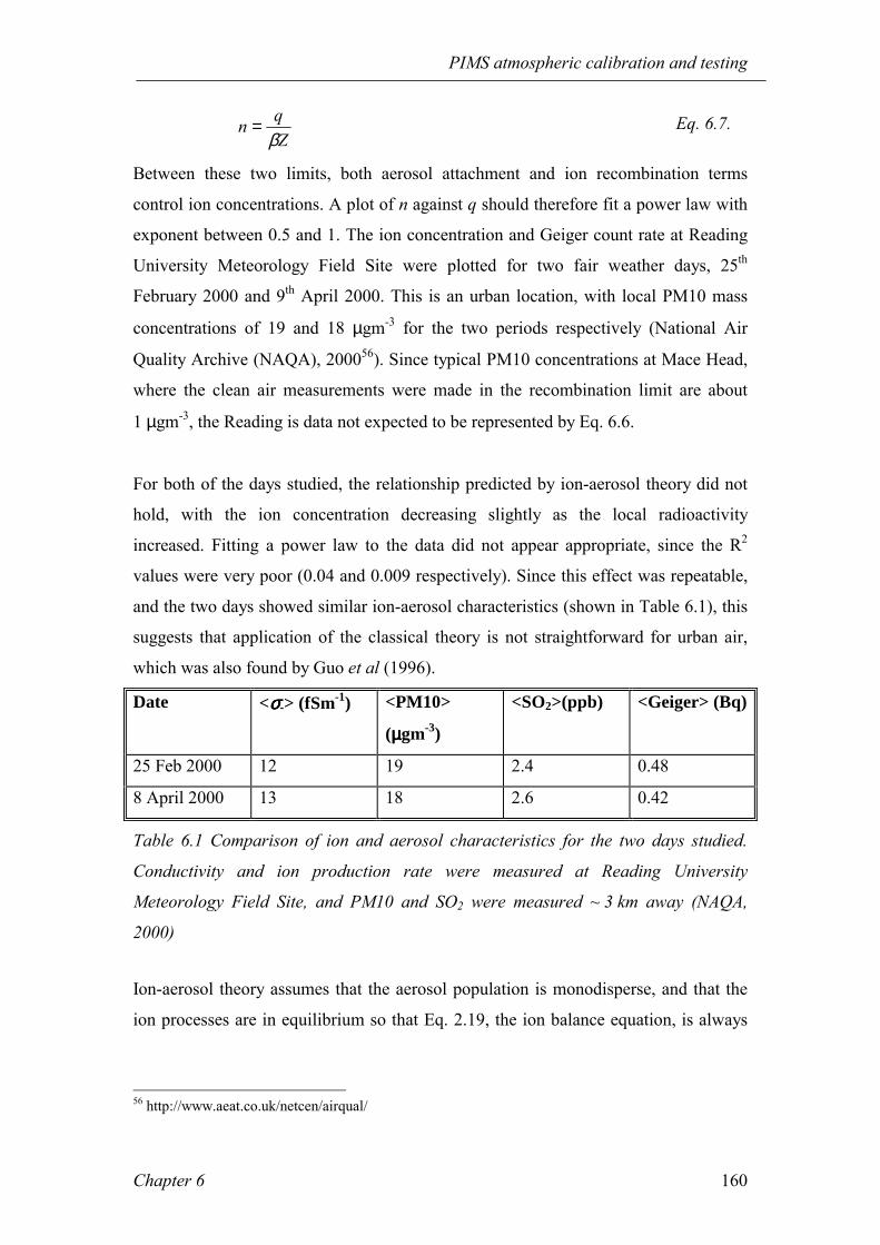
PIMS atmospheric calibration and testing
Chapter 6 160
Zqn
β= Eq. 6.7.
Between these two limits, both aerosol attachment and ion recombination terms
control ion concentrations. A plot of n against q should therefore fit a power law with
exponent between 0.5 and 1. The ion concentration and Geiger count rate at Reading
University Meteorology Field Site were plotted for two fair weather days, 25th
February 2000 and 9th April 2000. This is an urban location, with local PM10 mass
concentrations of 19 and 18 µgm-3 for the two periods respectively (National Air
Quality Archive (NAQA), 200056). Since typical PM10 concentrations at Mace Head,
where the clean air measurements were made in the recombination limit are about
1 µgm-3, the Reading is data not expected to be represented by Eq. 6.6.
For both of the days studied, the relationship predicted by ion-aerosol theory did not
hold, with the ion concentration decreasing slightly as the local radioactivity
increased. Fitting a power law to the data did not appear appropriate, since the R2
values were very poor (0.04 and 0.009 respectively). Since this effect was repeatable,
and the two days showed similar ion-aerosol characteristics (shown in Table 6.1), this
suggests that application of the classical theory is not straightforward for urban air,
which was also found by Guo et al (1996).
Date <σσσσ-> (fSm-1) <PM10>
(µµµµgm-3)
<SO2>(ppb) <Geiger> (Bq)
25 Feb 2000 12 19 2.4 0.48
8 April 2000 13 18 2.6 0.42
Table 6.1 Comparison of ion and aerosol characteristics for the two days studied.
Conductivity and ion production rate were measured at Reading University
Meteorology Field Site, and PM10 and SO2 were measured ~ 3 km away (NAQA,
2000)
Ion-aerosol theory assumes that the aerosol population is monodisperse, and that the
ion processes are in equilibrium so that Eq. 2.19, the ion balance equation, is always
56 http://www.aeat.co.uk/netcen/airqual/

PIMS atmospheric calibration and testing
Chapter 6 161
equal to zero57. However, even a very short 1 Hz Geiger time series, such as Figure
6.7, shows that q is extremely variable, and the classical average of 10 ion pairs cm-3s-
1 (Chalmers, 1967) is presumably a very long term average.
0
0.2
0.4
0.6
0.8
1
1.2
1.4
15 15.017 15.034 15.051 15.068
Time of day (BST)
Gei
ger c
ount
s (s
-1)
Figure 6.7 A four minute time series of 1 Hz Geiger counter data from Reading
University Meteorology Field Site on 8th April 2000, 1500-1504.
The great variability of q (an order of magnitude in a few minutes is normal, as in
Figure 6.7) perturbs the steady-state assumed by the ion balance equation. This makes
it more difficult to use ion-aerosol theory to show that the PIMS is actually
responding to ion variations, but its response to large fluctuations in ionisation can be
instead be used as a test. Long-term averages could also be used, but the Geiger count
rate does not vary in a very wide range, and the ion concentration is also sensitive to
other factors (e.g. aerosol concentration, meteorological effects), so it would be
difficult to distinguish the effect of the ionisation rate alone from the other quantities
influencing the ions. Figure 6.8 shows a comparison between the ionisation rate and
the ion concentration for a time series of one hour. Negative ions were measured with
the PIMS, at a bias voltage of 30 V, and the ion current (which is directly
proportional to the ion number concentration) is plotted with the count rate from an
adjacent Geiger counter at the same height (1.25 m).
57 Applying ion-aerosol theory to PIMS data will be discussed further in Chapter 7.

PIMS atmospheric calibration and testing
Chapter 6 162
0.3
0.35
0.4
0.45
0.5
0.55
0.6
16 16.25 16.5 16.75 17
time (BST)
Gei
ger (
s-1)
-0.35
-0.3
-0.25
-0.2
-0.15
-0.1
-0.05
0
PIM
S ne
gativ
e io
n cu
rren
t (pA
)
Geiger (157 pt moving av)current
Figure 6.8 PIMS 3 response to ionisation fluctuations. This is part of a time series
measured at Reading on 8th April 2000 from 1500-2100. 1600-1700 is shown here.
The thinner dotted trace (RH axis) is the negative ion current, sampled every 157s
and filtered according to the criteria discussed above. The thicker trace is a 157 point
centred moving average of 1 Hz Geiger counter data.
Some of the ion peaks, at about 1630, 1645 and 1700 occur at the same time as a peak
in the Geiger output, which suggests that the PIMS is able to respond to ionisation
fluctuations. The PIMS has now been demonstrated to respond to ionisation transients
in urban air on the timescale of minutes, which supports the clean air calibration
described in Section 3.3.2.
6.4 PIMS ion measurement mode intracomparisons The two PIMS measurement modes were compared by running both modes on one
instrument at the same bias voltage in fair weather conditions, and conductivity
calculated from both methods as described in Section 6.1. The two modes frequently
showed a good agreement, and an example is given below (Figure 6.9), in which the
correlation coefficient of 15-minute averages of the data is 0.51.

PIMS atmospheric calibration and testing
Chapter 6 163
-10
0
10
20
30
40
50
60
70
14 14.5 15 15.5 16 16.5 17
time (BST)
Con
duct
ivity
(fS/
m)
current method
decay method
Figure 6.9 Comparison of the two PIMS measurement modes on 9th April 2000 at
Reading. Results are shown from the PIMS 2 instrument from 1400-1700.
There is generally a correspondence in the trends of the two traces, e.g. from 1410-
1453, 1536-1648. Although there are some periods when the magnitudes of the two
traces agree well, e.g. 1424-1453, 1605-1634, their mean values are significantly
different. In Figure 6.9, the mean negative conductivity from the Current Method, σi,
was 10 fSm-1, but from the Voltage Decay mode, σv, it was 18 fSm-1. Both these
values are acceptable (see review of previous measurements in Section 2.2.3), but the
difference between them implies a variable offset or gain in one or both of the
measurement modes. As the gain of the MME is known to remain constant for times
of order months, and the offset terms show shorter-term variability, for example
temperature effects, this disparity is likely to be caused by leakage currents that have
not been fully compensated for.
6.4.1 Likely origin of conductivity offsets In the Current Measurement mode, it has been shown (Section 5.6.2) appropriate to
apply a correction based on the measured electrometer leakage current iL. In the MME
follower mode (the MME schematic is given in Figure 5.6, and a description of the
modes is in Appendix A) relays RL1, 5 and 2 are open, as shown in Figure 6.10. RL 2
has no current path and RL5 is guarded, therefore the follower mode leakage current

PIMS atmospheric calibration and testing
Chapter 6 164
iF will be the sum of the leakages at the input, from RL2 and the op-amp input bias
current. In the leakage check mode, which monitors op-amp bias and electrometer
leakage currents, the leakage current iL is contributed to by RL1, the op-amp input
bias current and leakages at the input.
RL1
a) Follower b) Leakage current check
-+ -
+
RF
ib
RL3to RL5
INRL2
RL2RL4
RL1
RL3
Figure 6.10 Differences between the MME follower and leakage current measurement
configurations a) and b). In this simplified diagram, an open relay is represented as a
capacitor, as it transiently injects charges when opening, and a closed relay (thick
line) is a direct connection.
As both iF and iL principally originate from leakage across one relay, they are likely to
be similar in magnitude. However, in the Voltage Decay mode, current is not
measured directly, and has to be inferred from the overall rate of decay. It can
therefore be assumed unnecessary to correct for the leakage current in this mode, as
long as the leakage can be considered to have a negligible effect on the rate of decay.
The contribution to the Voltage Decay mode conductivity σv from the electrometer
leakage current iL was calculated, and subtracted from σv. For the data shown in
Figure 6.9, this changed the conductivity by 2 %, indicating that the electrometer
leakage currents are only one-fiftieth the size of the ion signal, which is comparable to
the errors introduced from the bias voltage determination in Section 5.3. This shows
that the electrometer leakage measurement has no distinguishable effect on σv, given
its typical variability. Therefore, no corrections for electrometer leakage currents are
applied to the data from the Voltage Decay mode during processing.
PIMS atmospheric calibration and testing
Chapter 6 165
6.4.2 Negative conductivities A negative voltage repels negative ions flowing through the Gerdien tube towards the
central electrode. When the negative ions reach the central electrode they cause a flow
of electrons, and by convention (e.g. Bleaney and Bleaney, 1985) this leads to a
negative current58. Including the sign of the bias voltage, conductivity calculated from
Eq. 2.2 should always be a positive value. Hence, currents measured at the central
electrode should always be the same sign as the bias voltage, if they are entirely ionic
in origin. Yet Figure 6.9 clearly shows that the conductivity is sometimes negative,
because ic was the opposite sign to the bias voltage. The behaviour of the currents
when of the opposite sign to the bias still conform to the trend and correlate with σv.
This effect is therefore highly likely to be due to an offset imposed by some spurious
source of current. This current source can only originate from three places: the
electrometer, Gerdien tube itself, or some source of charge external to the PIMS
system. Tube leakage currents are caused by insulator degradation, or build-up on the
electrode surfaces. Although they probably do contribute some systematic error to the
measurements, the effect will be the same for both ion measurement modes, and is
unlikely to be the cause of the offset in the current mode. Electrometer leakage is a
possible contributor, but in the leakage checking mode, more relays are open than in
the current mode, which should exceed the leakage currents that are not compensated
for (see Section 5.6.2). To cause the persistent offset in Figure 6.9, the leakage from
one relay alone would have to be comparable to the ion current, so the likelihood of
this originating from the one relay which is not compensated for in the leakage
checking mode is probably small. It is therefore most likely that the offset in the
Current Measurement mode results from some external current source, and of a
similar magnitude to the ion currents.
6.4.3 Temporal inconsistencies Ion measurements in the two modes are made sequentially and are typically a minute
apart. If there are short-term fluctuations in the air passing through the PIMS, the
changes in the air being sampled may be detected by consequent measurements in the
two modes, which will introduce an error. There are significant turbulent fluctuations
58 An electrical current flows from positive to negative, but the flow of electrons is from negative to positive. Therefore a flow of negative charge is in the opposite direction to the current, so the current is negative.

PIMS atmospheric calibration and testing
Chapter 6 166
in the air of timescales from several minutes to milliseconds (Stull, 1997). As the
critical mobility is directly proportional to the wind speed, turbulence will continually
modify the fraction of the ion spectrum contributing to the measurement, and may
cause disparities between consecutive measurements in different modes. An
arbitrarily selected hour of 1 Hz wind data at Reading University Meteorology Field
Site, 1100-1200 on 12th June 2000, showed a maximum fluctuation of a factor of 4 on
a 30 s time-scale. Since the five minute average wind speed for this period was
3.4 ms-1, this corresponds to fluctuations in the range 6.8 1.7 ms-1. At a typical bias
voltage of 20 V, this causes changes in critical mobilities from 1.35 0.33 cm2V-1s-1,
spanning about half of the conventionally accepted small ion spectrum as defined by
Hõrrak et al (1999). This range is for a large fluctuation, but smaller variations in the
wind speed will also have some effect on the measurement. Critical mobility
variations due to the voltage decay itself will affect the radius of ions contributing to
the measurement. However this variation (which is a maximum of 2.5 V) will be
insignificant compared with the effect of turbulent fluctuations of wind speed, which
is the major factor contributing to the differences between the two measurement
modes. Further differences between the modes (as opposed to the differences in
measuring them), and the effect of wind fluctuations on the ion spectrum will be
discussed in Chapter 7.
6.5 PIMS systems intercomparisons Figure 6.11 and Figure 6.12 show the results of conductivity measurements using the
different PIMS devices by the two methods on two different fair weather days at
Reading.

PIMS atmospheric calibration and testing
Chapter 6 167
0
5
10
15
20
25
30
35
40
45
50
14 14.5 15 15.5 16 16.5 17time (BST)
nega
tive
cond
uctiv
ity /
fSm
-1
PIMS3PIMS2
Figure 6.11 Negative conductivity measured by the current method with PIMS 2 and 3
at Vb = -20 V on 9th April 2000 at Reading. Data shown is a filtered59 sample (12 % of
data set discounted) from 1400-1700.
0
5
10
15
20
25
30
35
40
11 11.5 12 12.5 13 13.5 14 14.5 15 15.5 16 16.5 17 17.5 18
time (BST)
fS/m
PIMS2PIMS1
Figure 6.12 Comparison of negative conductivities measured by the Voltage Decay
method with PIMS 1 and 2 at Reading on 18th June 2000. A seven-hour filtered time
series (35 % of data set discarded) is shown.
59 Filtering criteria are explained in Section 6.7.
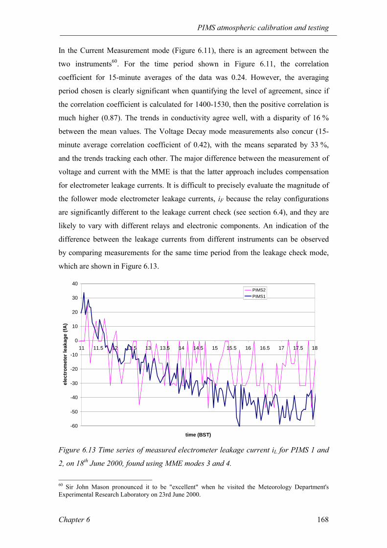
PIMS atmospheric calibration and testing
Chapter 6 168
In the Current Measurement mode (Figure 6.11), there is an agreement between the
two instruments60. For the time period shown in Figure 6.11, the correlation
coefficient for 15-minute averages of the data was 0.24. However, the averaging
period chosen is clearly significant when quantifying the level of agreement, since if
the correlation coefficient is calculated for 1400-1530, then the positive correlation is
much higher (0.87). The trends in conductivity agree well, with a disparity of 16 %
between the mean values. The Voltage Decay mode measurements also concur (15-
minute average correlation coefficient of 0.42), with the means separated by 33 %,
and the trends tracking each other. The major difference between the measurement of
voltage and current with the MME is that the latter approach includes compensation
for electrometer leakage currents. It is difficult to precisely evaluate the magnitude of
the follower mode electrometer leakage currents, iF because the relay configurations
are significantly different to the leakage current check (see section 6.4), and they are
likely to vary with different relays and electronic components. An indication of the
difference between the leakage currents from different instruments can be observed
by comparing measurements for the same time period from the leakage check mode,
which are shown in Figure 6.13.
-60
-50
-40
-30
-20
-10
0
10
20
30
40
11 11.5 12 12.5 13 13.5 14 14.5 15 15.5 16 16.5 17 17.5 18
time (BST)
elec
trom
eter
leak
age
(fA)
PIMS2PIMS1
Figure 6.13 Time series of measured electrometer leakage current iL for PIMS 1 and
2, on 18th June 2000, found using MME modes 3 and 4.
60 Sir John Mason pronounced it to be "excellent" when he visited the Meteorology Department's Experimental Research Laboratory on 23rd June 2000.

PIMS atmospheric calibration and testing
Chapter 6 169
The measured electrometer leakage currents varied significantly; for PIMS 1 the mean
leakage current was 26 fA, and for PIMS 2 it was 16 fA. As mentioned earlier, the
measured follower mode leakage current iF is only contributed to by one of the three
reed relays determining iL, so iF < iL, but iF /iL is probably constant, if it is assumed
that each reed relay contributes a constant amount of current into the system. So it is
not unreasonable to expect voltage decay measurements from two instruments (when
iF is negligible, but not precisely known) to agree less well than current
measurements, where iL is larger, but better-determined and compensated for.
6.5.1 Local variations between the PIMSs As different air, which is constantly fluctuating in turbulent eddies, is sampled by
each instrument, this will introduce some errors between the instruments due to local
variations. The mean eddy size l can be estimated from von Karmans constant, κ, at
the height of the instruments, z (Stull, 1997),
zl κ= Eq. 6.8.
Since κ = 0.4 and z = 1.5 m, then the mean eddy size is of comparable scale to the
instrument separation, suggesting there may be a significant spatial variation in the
wind speed, which may affect the ions sampled by the PIMS.
Leakage across the electrode insulation will vary from instrument to instrument, but
the three PIMS are mechanically very similar. Evidence for this is that the Gerdien
tubes only varied by 2 % in capacitance, which is an extremely sensitive parameter to
changes in dimensions (see Eq. 2.17). The variations in the bias voltage generator
have been included in the software, since each PIMS instrument was controlled by a
dedicated program with calibration differences accounted for (see Section 5.7.2). The
fans ventilating the tubes will also behave slightly differently, but these variations will
be small compared to the spatial effects of wind speed fluctuations. This appears the
most likely cause for the variability between instruments not attributed to leakage
currents.

PIMS atmospheric calibration and testing
Chapter 6 170
6.6 Comparing PIMS data to other ion measurements
6.6.1 Ion measurements made with another design of Gerdien Condenser Conductivity measurements made with the PIMS were compared to similar
measurements made with another Gerdien condenser of more classical design. This
design of instrument has been discussed by Blakeslee (1984) and widely applied, e.g.
by Anderson and Bailey (1991) and Blakeslee and Krider (1992). The instrument used
here was developed at the University of Arizona and will consequently be referred to
as the "Arizona Gerdien".
The PIMS and the Arizona Gerdien were set up adjacent to each other at Reading
University Meteorology Field site on a fair weather day. The response of the Arizona
Gerdien is given as 6.2 fSm-1V-1 at a bias voltage of 20 V(Blakeslee and Krider, 1992)
which (from Eq. 6.1) corresponds to a current amplifier sensitivity of 0.88 pAV-1.
A slight difference in the conductivities is to be expected from the two instruments,
because of their varying critical mobilities. The Arizona Gerdien is significantly
larger than the PIMS (a ~ 5 cm, b ~ 0.5 cm), therefore it is impossible to exactly
match the instruments critical mobilities given the practical limitations to bias
voltages and flow rates. In the absence of an ion mobility spectrum for the
measurement period, the difference between the measurements cannot be predicted.
Primarily for this reason, the Ohmic response of the Arizona Gerdien was measured;
an additional benefit is that this is a standard test that the Gerdien condenser is
responding to atmospheric ions (Chalmers, 1967). If the Gerdien condenser is in the
conductivity measurement régime, the mean conductivity can be calculated from the
gradient of the straight line fit to the Ohmic plot in Figure 6.14, m, which gives the
average output current to bias voltage ratio for the measurement period. Hence, from
Eq. 6.1 the conductivity is given by:
C
m 0εσ = Eq. 6.9.
Manual current measurements were made across the bias voltage range Vb = ± 11-
106 V. The output was logged on a Gould BS-272 chart recorder. Meanwhile, PIMS 3
measured negative conductivity at 0.5 Hz in the Current Mode. At the end of the

PIMS atmospheric calibration and testing
Chapter 6 171
PIMS logging period the Arizona Gerdien Ohmic response to negative voltages was
tested again. Results from the Ohmic response tests are in Figure 6.14.
y = 0.0252x + 0.0628R2 = 0.959
y = 0.0321x - 0.564R2 = 0.9173
y = 0.0508x - 0.5249R2 = 0.9633
-6
-4
-2
0
2
4
6
-120 -80 -40 0 40 80 120
bias voltage (V)
i out
(pA
)
2nd calibration
1st calibration
Calibration (positive)
Linear (2nd calibration)
Linear (1st calibration)
Figure 6.14 Ohmic response of Arizona Gerdien. The two tests at negative voltages
were made approximately an hour apart.
The linear response shows that the Arizona Gerdien was measuring conductivity at
this time. The negative conductivity for the first calibration was 36.0 fSm-1, and for
the second calibration 45.8 fSm-1. The average for the two-hour measurement period
is 40.9 fSm-1. A sample of the Arizona Gerdien chart recorder output is given below.

PIMS atmospheric calibration and testing
Chapter 6 172
0 V
5 V
4 s
Figure 6.15 Sample of the Arizona Gerdien output at Vb = -105 V. The chart recorder
trace is centred at 0 V, and axis scaling is indicated on the trace.
The PIMS output (Figure 6.16) appears similar to the Arizona Gerdien trace (Figure
6.15). This suggests that the noise is independent of the instrument, and atmospheric
ions may be a fundamentally noisy quantity. The main processes affecting the
atmospheric ion concentration: production, attachment and recombination are all
constantly fluctuating in rate because of atmospheric turbulence and the stochastic
nature of ionisation processes. The air sampled by the instruments is also rapidly
changing in its qualities, because of the variability in the ion concentration discussed
above, and turbulent eddies affecting the origin of the air sampled61. However, the
mean conductivities from the two instruments agree well: the PIMS mean
61 Variability in the measurements will be discussed further in Chapter 7.

PIMS atmospheric calibration and testing
Chapter 6 173
conductivity was 41.6 fSm-1, which is less than 2 % higher than the average Arizona
Gerdien conductivity. It can be concluded that the PIMS can measure conductivity to
within 2 % of the conductivity measured by a reference Gerdien condenser.
0
20
40
60
80
100
120
140
15.35 15.4 15.45 15.5 15.55 15.6time (BST)
fSm
-1
Figure 6.16 Sample of PIMS 0.5 Hz negative conductivity trace.
6.7 Average conductivities Ion measurements in the literature are usually presented as average values, although
the amount of data averaged is often reasonably small, which suggests that textbook
values should not necessarily be equated with reliability. In fact there is significantly
more data presented in this Thesis than in much classical work on the subject (e.g.
Chalmers, 1967) 62. To compare the PIMS conductivity data from Reading University
Meteorology Field Site with such historical averages, data from the continuous
measurement campaign from April June 2000 was averaged. Measurements were
only attempted on fair weather days, so that the atmospheric electrical conditions
would be relatively unperturbed by the presence of hydrometeors and aerosol
(Barlow, 2000). The definition of fair weather was based loosely on Reiters
criteria, discussed in Barlow (2000), who concluded that there was a need for 62In the group led by Chalmers at Durham (where I was an undergraduate in the Physics Department, and Atmospheric Electrical work had sadly long since ceased) in the 1960s, two days of consistent atmospheric electrical data was then considered an adequate amount for a PhD. Thesis (Jones, 1999).

PIMS atmospheric calibration and testing
Chapter 6 174
redefinition of the term based on micrometeorological considerations. For the results
presented here, the major consideration for starting a run of measurements was that
there was less than 3/8 cloud cover, which was typically fair weather cumulus.
The conductivity data were hourly averaged (<σ>), and then filtered based on the
following criteria.
• <σ> > 2iL is a pragmatic treatment of the errors introduced by leakage. The
measured leakage current iL is not a full compensation for the electrometer
leakage, because there is one reed relay unaccounted for between the MME
current measurement and leakage check modes. Since iL is mostly leakage from
one relay (see discussion in Section 6.4.1), but its sign is not known, 2iL is
therefore a conservative estimate for the uncompensated leakage current.
• <σ> < 50 fSm-1 excludes measurements that are larger than the theoretical
maximum ion concentration, for q = 10 cm-3s-1. In the recombination limit the
maximum ion concentration can be easily calculated from Eq. 6.6, which gives an
upper limit of 2500 ions cm-3. Since
µσ ne≈ Eq. 6.10,
and the mean mobility of atmospheric small ions is 1.2 cm2V-1s-1 (e.g. Dolezalek,
1974), then σmax ~ 50 fSm-1. This is an absolute maximum upper limit, since it
assumes an aerosol-free atmosphere, and any aerosol present (which there clearly
is in urban Reading air) reduces the ion concentration.
Conductivity values outside these limits are spurious, and caused by non-ionic current
sources dominating the signal. When the conductivity is within the acceptable range,
there may still be offsets contributing to the measurement, but the filtering criteria
described above only include measurements when the offset is small. Averaging the
remaining data will further reduce the error due to random offsets.
Measurements were made with the three PIMS on the mast at 1.25 m (see Figure 6.2)
on 24 days in April, May and June 2000 for 292 hours. The total logging time is an
average across the three PIMS instruments; they ran for similar lengths of time, but Although the acquisition of data is now more straightforward, the frequency of suitable fair weather days is unlikely to have changed by orders of magnitude.

PIMS atmospheric calibration and testing
Chapter 6 175
this varied slightly as individual PIMS were removed for cleaning and repair. The
measurement periods were limited by the weather conditions, for example in April
2000, which was the wettest month since 1756 (Eden, 2000a) fair weather was rare
and the instruments were only run for 85 hours. In May, the first half of the month
offered some good measurement days (Eden, 2000b), though continual (inaccurate)
predictions of thunder meant the logging strategy had to be conservative to avoid
possible lightning damage from transients to the circuitry. It is an unfortunate
vicissitude of the British climate that fair weather days in the spring and summer,
which are favourable for atmospheric electrical measurements, are when the
convective activity which leads to thunderstorms is most likely. The apparent need of
weather forecasters to alert the public to even the slightest risk of thunder presents a
further problem, since instruments designed to measure fair weather quantities (like
the PIMS) may not be able to withstand the dramatic changes associated with
thunderstorms. Measurements were therefore abandoned when thunder was predicted,
which lost considerable logging time during fair weather, as well as the periods when
the instruments were being maintained.
After the filtering criteria described above had been applied to the whole set of hourly
averages, 50 % of the data were retained. The efficiency of the two modes was
different, with 63 % of current mode data retained after filtering and 36 % of the
Voltage Decay mode results. The voltage decay data was generally noisier and gave
conductivities which were greater in magnitude than those from the current mode.
This is summarised in the mean data shown in Table 6.2 below, where the voltage
decay mean and standard deviation are greater than in the current mode. The average
air conductivity in the literature63 lies between the means for the two modes at 13
fSm-1, but is obviously close to the current mode measurements.
63 This is calculated from the values given in Table 2.1

PIMS atmospheric calibration and testing
Chapter 6 176
Measuring
Mode
Mode efficiency
(% data retained) <σσσσ> (fSm-1) <standard
error> (fSm-1)
Current 63 12 3
Voltage 36 19 7
Table 6.2 Summary of conductivity measurements from three PIMS running in two
modes. Conductivities were averaged across all instruments for the periods when
more than two PIMS were running.
0
10
20
30
40
50
0 6 12 18 24
time (UTC)
nega
tive
cond
uctiv
ity (f
S/m
)
Current methodDecay method
Figure 6.17 Average diurnal variation in conductivity calculated by the two methods.
Error bars are the standard error of the mean for each set of hourly averages, for
three instruments.
Figure 6.17 shows the hourly conductivity averages, taken over 292 hours on 24 days
and averaged across the PIMS instruments. The trends in conductivity calculated by
the two methods agree well, though the mean values differ. The pattern of this
diurnal variation is similar to those in the literature, discussed in Section 2.2.3, with a
pre-sunrise peak at 0400-0500, due to a maximum in the ionisation rate caused by
thermal stratification. Throughout the day conductivity then decreases, which is
traditionally explained by the wind increasing after midday and turbulent mixing
dispersing the radioactive gases contributing the majority of the ionisation (Chalmers,
1967). As in Section 2.2.3, studying the trace from a local Geiger counter, which is a

PIMS atmospheric calibration and testing
Chapter 6 177
proxy for the majority of the ionisation rate, can give some insight into this. The
Geiger counter output and the global solar radiation for an example day, 19th October
1999, are shown in Figure 6.18; from midnight to sunrise there is an increasing
ionisation rate, which is at its maximum during sunrise. This is probably caused by
the stable nocturnal surface layer trapping radioactive gases emitted from the soil
(such as radon), which cause most of the ionisation at the surface64.
64 Comparison between the ion production rate and the ion concentration is more complicated during the day, because aerosol concentrations and wind speeds are more variable. This has been discussed in Section 2.2.3.

PIMS atmospheric calibration and testing
Chapter 6 178
0
100
200
300
400
500
0 4 8 12 16 20 24time (UTC)
Sola
r rad
iatio
n / W
m-2
0.3
0.35
0.4
0.45
0.5
Gei
ger c
ount
s / s
-1
Global solar radiationGeiger counter output30 min Geiger running mean
Figure 6.18 Five minute averages of global solar radiation (left hand axis) and
Geiger count rate (right hand axis) for 19th October 1999 at Reading University
Meteorology Field Site. A 30 minute running mean of the Geiger counter trace is also
shown.
0
2
4
6
8
10
12
14
0 4 8 12 16 20 24
time (UTC)
tem
pera
ture
/ de
gree
s C
elsi
us
0
1
2
3
4
5
6
wind speed / m
/s
-1
Td degC Tw degC u (m/s)
Figure 6.19 Five minute averages of wet (Tw) and dry-bulb (Td) temperatures at 1 m,
and wind speed (u) at 10 m for the same example day, 19th October 1999.
PIMS atmospheric calibration and testing
Chapter 6 179
6.8 Conclusions This chapter has shown that the PIMS devices can measure ions consistently in both
the Current Measurement and Voltage Decay modes. The instrument responds to
fluctuations in the ionisation rate, and there is good agreement across both modes with
the same instrument, and between the three PIMSs. Some of the disagreements
between the instruments have been explained in terms of spatial and temporal
inconsistencies in the air being sampled. The conductivity trends also agree with those
recorded by another Gerdien instrument. The average diurnal variation found over 24
days in a three-month period is concomitant with previous measurements, and many
of its variations can be explained in terms of meteorological factors.

Variability in PIMS measurements
Chapter 7 180
the fact that an experiment delivers an unexpected answer means simply that you have not asked the question you assume you have asked C.L. Stong65
7 Variability in PIMS measurements The aim of this chapter is to resolve some uncertainties in the PIMSs data so that a set
of operating conditions can be defined during which the PIMS is measuring small
ions. In Chapter 6, it was suggested that the presence of charged particulates may
have a deleterious effect on the measurements. This is analysed in detail, and other
sources of error are investigated to further refine the operating conditions.
7.1 Effect of fluctuations in the flow
7.1.1 The contribution of intermediate ions to conductivity The critical mobility is directly proportional to the wind speed (Equation 2.11), so at
lower wind speeds the size of ion contributing to the conductivity measurement
increases. It can be hypothesised that greater conductivity is observed at night, when
there is low wind in the stable nocturnal boundary layer (Stull, 1997), simply because
intermediate ions are contributing to the measurement. This was tested using data
from a fair weather day, 3 May 2000 when there was a 24-hour set of hourly averaged
conductivity data, which itself conformed to the diurnal variation frequently cited in
the literature (Section 2.2.3). The maximum radius of ion contributing to the
measurement, rmax, was calculated as in Section 3.2.2. The wind component inside the
tube was calculated from Eq. 3.11 and Eq. 3.12. The diurnal variation of negative
conductivity and rmax are shown in Figure 7.1. It is clear that almost all of the peaks in
conductivity coincide with maxima in rmax, when it is therefore possible that more
ions are contributing to the conductivity. For the day chosen, the conductivity is
principally due to conventional small ions for the whole day, but at lower wind speeds
rmax could easily encroach into the intermediate ion size range of r > ~ 1 nm (Hõrrak
et al, 2000), as also discussed in Section 3.2.2. This is important to recognise, because
a significant contribution of intermediate and large ions to the conductivity has been
theoretically shown to invalidate the traditional conductivity-aerosol relationship (see
Section 2.4) by Dhanorkar and Kamra (1997).
65 The Amateur Scientist, Heinemann, London (1965)

Variability in PIMS measurements
Chapter 7 181
0
0.1
0.2
0.3
0.4
0.5
0.6
0.7
0.8
0.9
1
0 4 8 12 16 20 24
time (BST)
max
imum
ion
radi
us (n
m)
0
5
10
15
20
25
30
35
40
nega
tive
cond
uctiv
ity (f
S/m
)
maximum ion radiusconductivity
Figure 7.1 Diurnal variation of conductivity (hourly averages of both methods, for a
period when their results agreed) and maximum ion radius (calculated from 5 minute
averages of wind component) for 3 May 2000.
If the measured ion size is not considered, as is conventional, the contribution of
larger ions can be misleading. They could make the measurements appear as if they
are conforming to the expected patterns, when in reality they are only reflecting the
fraction of the ion spectrum contributing to the measurement rather than the ion
concentrations. The conventional expression for conductivity (Eq. 2.14) can be
rewritten to take account of this
LLii enenne µµµσ ++≈ Eq. 7.1,
which separates the contribution of the intermediate and large ions. Ideally, in
conductivity measurement, the intermediate and large ions can be ignored when there
are few of them because their mobilities are orders of magnitude lower than small
ions, and their contribution is negligible. Here it is shown that under certain
circumstances, intermediate ions can be measured in such numbers that they do
contribute to the conductivity measurement. Classical ion-aerosol theory only holds
when the conductivity is entirely due to small ions, because intermediate and large
ions are effectively charged aerosol particles (Hõrrak et al, 2000), so the spectral
separation between them becomes indistinct. Hence, for different conductivity

Variability in PIMS measurements
Chapter 7 182
measurements to be comparable, it is necessary to ensure that the conductivity is only
contributed to by small ions.
If rmax is calculated from wind measurements made near to the ion measurement site,
this problem can be alleviated by discarding data where rmax falls into the intermediate
ion range. 1 Hz wind speed and direction measurements are made continually at 10 m
at the Field Site, and five-minute averages from these data were used to rescreen the
ion data presented in Section 6.6.2. A further five hours of data were rejected on
average for each PIMS, which reduced the total amount of data available for analysis
by a further 2 %. The revised diurnal variations are shown in Figure 7.2, where the
conductivity traces from the two methods are in better agreement both in magnitude
and in trends (this is summarised in Table 7.1). The correlation coefficient between
conductivities calculated by the two methods is 0.51, which is improved compared to
the correlation when the contribution of intermediate ions was ignored (0.34).
0
10
20
30
40
50
0 6 12 18 24
time (UTC)
nega
tive
cond
uctiv
ity (f
S/m
)
Current method, rmax filtered
Decay method, rmax filtered
Decay method, chapter 6
Current method, chapter 6
Figure 7.2 Average diurnal variation of negative conductivity, calculated as in
Chapter 6, but with further filtering to remove data where intermediate ions were
contributing to the measurement. The averages calculated without excluding
rmax > 1 nm (as in Chapter 6) are shown as dotted lines.

Variability in PIMS measurements
Chapter 7 183
Mode Mode efficiency
(% data retained) <σσσσ> (fSm-1) <standard
error> (fSm-1)
Current 61 13 4
Voltage 35 19 8
Table 7.1 Mean negative conductivities by the two methods after further filtering to
remove the contribution of intermediate ions.
The majority of changes in the average data compared to Chapter 6 are during the
night, when the wind speeds drop and larger ions are therefore more likely to be
captured. Since the data from the daytime remains largely unmodified, the poorer
agreement between the two modes in the daytime is a consequence of turbulent gusts
of wind affecting the ion concentration between consecutive measurements. As the
atmospheric surface layer is more stable at night, there is better temporal agreement
between measurements made asynchronously. It is clearly possible for intermediate
ions to contribute to the conductivity during still periods, particularly at night. I
believe, therefore, that this filtering procedure needs to be applied to all conductivity
measurements where the Gerdien condenser is susceptible to fluctuations in
ventilation. Some filtering of existing data for rmax may be necessary with this factor
in mind. Reanalysis of historic measurements has been previously shown to be
effective at improving conductivity measurements (Gunn, 1960; Andersen and Bailey,
1991)66.
7.1.2 Effect on the fraction of ions measured Measurement of wind speed and direction, and careful filtering of data should remove
the effect of intermediate ions (r > 1 nm (Hõrrak et al, 1999)) from analysed ion data,
because the times when they are contributing to the measurement can then be
identified. However, any change in wind speed causes a variation in the maximum
radius of ions being measured, and hence a change in the fraction of the ion spectrum
which is being observed. The variation of ion radius with external ventilation is
shown below in Figure 7.3. rmax is derived from the flow rate in the tube, calculated as 66 Gunn (1960) corrected conductivity measurements from the Carnegie cruises in the 1930s for errors due to the inlet pipes. Although inlet ducting will damp the effects of turbulent fluctuations in wind

Variability in PIMS measurements
Chapter 7 184
in Section 3.2.1. The plot is asymmetrical because of the fan sucking air through the
tube, which causes the flow rate in the tube to change depending on the direction of
the external wind.
0
0.5
1
1.5
-5 -4 -3 -2 -1 0 1 2 3 4 5
u component into tube uext / ms-1
r max
(nm
)
Figure 7.3 Maximum radius of measured ions with the external ventilation of the
Gerdien tube, at a typical bias voltage of 20 V. Flow in the tube is calculated from a
polynomial fit to the external flow rate, and radius is calculated from a simple power
law fit to approximate Tammets (1995) expression.
Figure 7.3 immediately shows that measurements made at very low flow rates permit
intermediate ions to contribute to the conductivity, and must be discarded. It also
shows that there is a significant variation in the radius of ion contributing to the
measurement, even when small ions only are being measured. This will cause some
uncertainty, but its magnitude will depend on the characteristics of the ion mobility
spectrum. For example, there is a steep change in the radius of the ions measured
between flows of 0 and -1 ms-1. If there is no variation in the number of ions with
radii between 1.1 and 0.8 nm, there will be no effect. If there is a significant
difference in the number of ions at the different radii, relatively small fluctuations in
the wind speed can cause a large error in the apparent determination of ion
concentrations. This error can be called the spectrum error, and its magnitude can
speed, thus reducing the need for the PIMS correction described here, it reduces the instruments collection efficiency (see Section 2.3).

Variability in PIMS measurements
Chapter 7 185
be estimated from a long-term average negative ion spectrum (Hõrrak et al, 2000),
which is shown in Figure 2.11. Assuming this as a reference spectrum, the errors in
the measurement of negative ion number concentration for 1 ms-1 step changes in
external ventilation are shown below.
0
10
20
30
40
50
-5 to -4 -4 to -3 -3 to -2 -2 to -1 -1 to 0 0 to 1 1 to 2 2 to 3 3 to 4 4 to 5
Change in external ventilation (m/s)
% c
hang
e in
num
ber c
once
ntra
tion
of n
egat
ive
ions
Figure 7.4 Estimated spectrum error at a bias voltage of 20 V, from 1 ms-1 changes in
external ventilation.
Figure 7.4 gives an estimate of the error in the measurement due to the non-uniform
nature of the ion mobility spectrum. At higher wind speeds rmax is lower, but the
PIMS is measuring in a steeper part of the ion mobility distribution so there is a
greater variation in the size of ion measured in a 1 ms-1 range of wind speeds. The
least desirable range of external wind components is from 0 to -1 ms-1, because in this
range the ions measured change from intermediate to small, and rmax is quite sensitive
to wind speed. Although the spectrum is flat from 0 1 ms-1, intermediate ions are
making up the majority of the conductivity so this data should be discounted.
Conductivity measurements when there is high external ventilation (i.e. for the PIMSs
orientation used in this Thesis experiments, strong southerly winds) should be treated
with caution, because errors are introduced as the number of ions being measured
varies sharply with wind speed. The most favourable wind speeds for conductivity

Variability in PIMS measurements
Chapter 7 186
measurement are moderate ones in the range 1-3 ms-1, which permit measurement of
small ions in a relatively smooth part of the spectrum.
7.2 Physical differences between the modes In the Current Mode, some preliminary averaging is carried out by the microcontroller
before the sample is sent to the logging PC. In the Voltage Decay mode, conductivity
is calculated from an exponential fit to 10 2 Hz samples. If a transient occurs, for
example a charged aerosol particle advected onto one of the Gerdien electrodes, this
will cause a perturbation to the electrical charge of the central electrode which is
proportional to the charge of the particle. If this occurs whilst current measurements
are being made, the transient effect is likely to be smoothed out by averaging, and
contributes little to the current. In the Voltage Decay mode, the charge on the central
electrode is logged at twice the speed, for half the time67, so any transient is likely to
be measured and sent serially to the PC where it may cause the fluctuations in the
decay time series shown in Figure 6.6. A fluctuation of 1 V can be estimated to
cause the voltage decay trace, which has a maximum range of 2.5 V, to deviate
considerably from the expected exponential. This is equivalent to a charged aerosol
particle carrying picoCoulombs and impacting on Gerdien electrodes (the Gerdien
condenser typically has a capacitance of 10 pF). Aerosol which is not in steady-state,
or is in a new region of ionisation, for example particles less than a few minutes old
(Harrison, 1992) can be charged highly enough (i.e. 10 pC), to cause such
perturbations. If one decay measurement lasts for 5 s, then a volume of about 5 x
10-3 m3 of air passes through the Gerdien, assuming a flow rate of 2 ms-1. As 60 % of
the voltage time series have a positive <∆V/∆t>, then this corresponds to about one
failure case per 100 m3 of air. This is equivalent to one charged particle per 5 m edge
cube of air, which appears a possible explanation for the observed proportion of non-
exponential decays. In addition to non-equilibriated aerosol particles, there are
numerous other air-borne sources of highly charged particles, for example a bumble-
bee (bombus terrestris) can carry 50 pC (Harrison, 1997b), and highly-charged
particles can be produced by mechanical processes.
67 The logging strategy has been described in detail in Section 5.6.3

Variability in PIMS measurements
Chapter 7 187
7.3 Offset currents measured at zero bias voltage When there is zero bias voltage Vb across the Gerdien electrodes, the ionic current
measured should be negligible, since there is no electric field in the tube. The only
ions which will be measured are those which collide with the electrodes by chance
due to mechanical motions. MacGorman and Rust (1998) refer to the process of
correcting the ion current by subtracting this zero current as dynamic zeroing. They
suggest it is the best way to zero the Gerdien system since it accounts for ionic noise
in the tube. However, this ionic noise signal is likely to be negligible compared to the
contribution also present from larger charged particles. Aerosol particles easily carry
several units of electronic charge (Clement and Harrison, 1992), and can be
influenced by mechanical forces. So the current when Vb = 0 should give an estimate
of the noise levels due to the presence of chance ionic and particulate, impaction onto
the electrodes.
The current at the central electrode when Vb = (0 ± 1) V, which will be referred to
here as iV=0 was measured for 43 hours of fair weather using PIMS 2 at Reading
University Meteorology Field Site from 2 - 4 May 2000. The same instrument also
measured the currents at Vb = + 25.0 and Vb = 19.8 V. The first observation was that
iV=0 was comparable in magnitude with currents measured at the higher voltages (here
called iV=-20 and iV=+25), which suggests that it is possible for particles in the tube to
cause a significant offset in the measurements. iV=0 also showed a close agreement
with both iV=-20 and iV=+25, and a time series of iV=0 and iV=+25 is plotted below to
illustrate this. Since electrical forces seem to have no effect on the current measured,
there must be a mechanical process acting in both cases.

Variability in PIMS measurements
Chapter 7 188
-1.0
-0.5
0.0
0.5
1.0
1.5
2.0
123.7 123.95 124.2 124.45 124.7 124.95 125.2 125.45
year day
curr
ent (
pA)
I (Vb = 0V)I (Vb = 25V)
Figure 7.5 Comparison of the currents measured with PIMS 2 when Vb = 0 and
Vb = 25 V from 1730 2nd May 2000 to 1130 4th May 2000. The x-axis divisions are 6
hours.
One approach which can be adopted is to investigate the distribution of the noise
current. A random source of errors is Gaussian in distribution (Horowitz and Hill,
1994), and if there are other processes affecting iV=0, then the distribution will not be
Gaussian. The distribution of iV=0 for the same data set plotted in Figure 7.5 was
calculated for two contrasting cases. The first case is when iV=0 is clearly dominating
the signal, defined by the presence of a negative current when the PIMS should only
be responding to positive ions. The second case is the average distribution for the
whole time series. The distributions are plotted in Figure 7.6 below. For the whole
time series, the distribution is approximately Gaussian, although there is a slight bias
in the tail towards positive currents. The peak is in the current bin of 0 0.2 pA,
which shows that the iV=0 signal is small for most of the time. The distribution when
iV=0 is large however, is much less symmetrical, with more frequent negative currents,
and less frequent positive currents. The peak is broad and spans larger negative
currents than the average distribution. This asymmetry shows that the noise has a non-
Gaussian distribution (Berthouex and Brown, 1994) when it dominates the signal at
larger bias voltages, compared to the mean distribution of iV=0. This suggests that iV=0

Variability in PIMS measurements
Chapter 7 189
is not random noise but is symptomatic of a more ordered process, bringing in
negative charge.
0
0.05
0.1
0.15
0.2
0.25
0.3
0.35
-0.7 -0.5 -0.3 -0.1 0.1 0.3 0.5 0.7 0.9 1.1 1.3 1.5 1.7 1.9
current bin (0.2 pA width)
N (i
) / fr
actio
n of
tota
l
All dataNoise dominated caseGaussian(all data)Gaussian (noise dominates)
Figure 7.6 Distribution of currents at Vb = 0 for the whole measurement period, and
for the period when iV = 0 is dominating the ion signal. The relative number of
occurrences of each current is plotted against the mean current of the 0.2 pA bin, e.g.
N(i) at 0.5 pA represents the fraction of readings for which a current between 0.2 and
0.4 pA was measured. Gaussian fits to the distribution are also shown. Correlation
coefficients to a Gaussian distribution for the whole data set and the case where noise
dominates were 0.98 and 0.95 respectively.
Having now established that iV=0 can be an important source of noise in the
measurements, the characteristics of the signal were investigated further. In the period
when iV=0 was considered to be dominating the signal, it showed a good agreement
with the wind component into the PIMS, illustrated in Figure 7.7. This strongly
implies that the origin of the dominant negative current is being blown into the tube
by the wind.

Variability in PIMS measurements
Chapter 7 190
-0.9
-0.7
-0.5
-0.3
-0.1
0.1
0.3
0.5
125.2 125.25 125.3 125.35 125.4
year day
curr
ent (
pA)
-4.00
-3.50
-3.00
-2.50
-2.00
-1.50
-1.00
-0.50
0.00
win
d co
mpo
nent
in tu
be (m
/s)
current (0V)wind component
Figure 7.7 A 4 hour 50 minute section of the iV = 0 time series (left hand axis) plotted
against 5 minute averages of the wind component into the tube (right hand axis).
A possible origin for the high currents observed at Vb = 0 is particulate space
charge68 drifting on to the Gerdien condenser electrodes. Space charge was measured
at Reading University Meteorology Field Site with an Obolensky-type device69, on
25th February 2000. Ion measurements with PIMS 1 at a bias voltage of 30.7 V were
also made. A time series of conductivity and the uncalibrated (negative) space charge
meter output, plotted in Figure 7.8 below, indicates a positive relationship between
the two quantities. This shows that the Gerdien condenser can respond to space charge
for at least the measured period. However, the contribution of space charge to the
conductivity measurement cannot be determined, as the exact response of the space
charge instrument is not known. In order to ascertain the magnitude of the
contribution, the partitioning of the space charge between aerosol and ions would also
need to be understood. Since conductivity measurement by definition directly 68 Space charge is a generic term for all the free charge per unit volume carried on particles in the air. It is partitioned between the charge carried by aerosol particles and small ions (Chalmers, 1967). 69 The Obolensky (1925) space charge meter uses a filter to collect the space charge so that the current from it can be measured. Obolensky (1925) used cotton wool, but the instrument fabricated and deployed at Reading uses steel wool as the filter. The tube used was approximately 20 cm long and 2 cm in diameter, ventilated with the same fan as the PIMS at an approximate flow rate of 2 ms-1. The
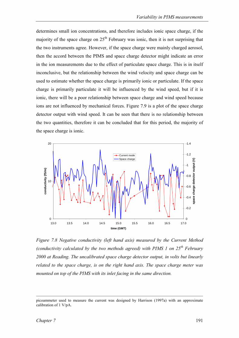
Variability in PIMS measurements
Chapter 7 191
determines small ion concentrations, and therefore includes ionic space charge, if the
majority of the space charge on 25th February was ionic, then it is not surprising that
the two instruments agree. However, if the space charge were mainly charged aerosol,
then the accord between the PIMS and space charge detector might indicate an error
in the ion measurements due to the effect of particulate space charge. This is in itself
inconclusive, but the relationship between the wind velocity and space charge can be
used to estimate whether the space charge is primarily ionic or particulate. If the space
charge is primarily particulate it will be influenced by the wind speed, but if it is
ionic, there will be a poor relationship between space charge and wind speed because
ions are not influenced by mechanical forces. Figure 7.9 is a plot of the space charge
detector output with wind speed. It can be seen that there is no relationship between
the two quantities, therefore it can be concluded that for this period, the majority of
the space charge is ionic.
0
10
20
13.0 13.5 14.0 14.5 15.0 15.5 16.0 16.5 17.0
time (GMT)
cond
uctiv
ity (f
S/m
)
-1.4
-1.2
-1
-0.8
-0.6
-0.4
-0.2
0
spac
e ch
arge
det
ecto
r out
put (
V)
Current modeSpace charge
Figure 7.8 Negative conductivity (left hand axis) measured by the Current Method
(conductivity calculated by the two methods agreed) with PIMS 1 on 25th February
2000 at Reading. The uncalibrated space charge detector output, in volts but linearly
related to the space charge, is on the right hand axis. The space charge meter was
mounted on top of the PIMS with its inlet facing in the same direction.
picoammeter used to measure the current was designed by Harrison (1997a) with an approximate calibration of 1 V/pA.

Variability in PIMS measurements
Chapter 7 192
y = 0.0965x - 1.6907R2 = 0.0758
-2
-1.8
-1.6
-1.4
-1.2
-1
-0.82 2.5 3 3.5 4 4.5
wind component / ms-1
spac
e ch
arge
det
ecto
r vol
tage
/ V
Figure 7.9 Space charge detector voltage as a function of wind component into the
space charge detector, for the same time period as Figure 7.8.
For the measurements made on 2 - 4 May 2000 at Vb = 0, the overall distribution was
close to Gaussian and the magnitude was small. This indicates that iV=0 is randomly
generated noise, the effect of which can therefore be reduced by averaging. However,
the same signal as that recorded at iV=0 sometimes dominates the measured ion signal
at higher bias voltages, and can cause a large enough offset for the measured currents
to be the opposite sign to the bias voltage. For these periods iV=0 shows a close
agreement with the external wind component. It is therefore almost certain that when
the current is the opposite sign to Vb, the source of the noise causing it (measured at
Vb = 0) is carried by the wind. On a different day (25th February 2000), space charge
was also related to the ion signal (correlation between 15-minute averages was 0.23),
in which there were no periods of large offset. Since the space charge was unrelated to
the wind speed on this day (Figure 7.9), then it must have been primarily ionic in
composition. In the example of the noise dominating the ion signal plotted in Figure
7.7, there is evidence that additional negatively charged particles blown in by the
wind are the source of the noise. According to Kamra (1992), negative space charge is
carried by the wind, so the results presented here confirm his hypothesis.

Variability in PIMS measurements
Chapter 7 193
The problem of particulate space charge contributing to the conductivity measurement
is likely to be worst when there are high aerosol concentrations, as there are lower ion
concentrations due to attachment. The combination of a greater proportion of charged
aerosol causing more noise, and the associated reduced ion signal will diminish the
signal-to-noise ratio. Early radiosonde measurements of voltage decays outside the
boundary layer (Hatakayema et al, 1958; Venkiteshwaran, 1958) had a high
proportion of successful decays, unlike the PIMS measurements at ground level. This
supports the concept that the PIMS measurements are perturbed by charged aerosol
particles being blown into the Gerdien tube, as aerosol concentrations fall with height
(Pruppacher and Klett, 1997). The effect of particulate space charge is thought to be
the principal source of noise in the instrument.
In the ion measurements presented above and in Chapter 6, the approach to filtering
was to prevent currents with a large non-ionic offset from being considered as small
ion measurements. The screening procedure used in Section 6.7 was appropriate for
this purpose, because it has excluded measurements when the noise currents were
large. A better criterion for data filtering would be to exclude data where the space
charge was known to be particulate, which would eliminate all ion measurements
containing a contribution from particulate space charge.
7.4 Ionic sources of noise
7.4.1 Atmospheric ion fluctuations The main source of ionic noise is fluctuations in the ion concentration itself - here
called ionisation noise. The ion production rate, measured with a Geiger counter,
shows high short-term variability (see Figure 6.7 for an example time series).
Fluctuations in the ion concentration are damped by self-recombination and
attachment to aerosol, but ion-aerosol timescales to reach steady-state concentrations
are of order 100 s (Harrison, 1992). As it takes about one-eighth of a second for an
ion to be sucked through the Gerdien at typical flow rates, the effects of a local
transient in the ion production rate are likely to be detected before a local steady-state
in the tube has been reached. Further evidence for the sensitivity of the instrument to
ionic fluctuations has been observed directly by sealing the ends of the Gerdien
condenser and measuring the current. On a chart recorder trace, small peaks can be

Variability in PIMS measurements
Chapter 7 194
seen, which must be attributed to individual ionisation events in the tube, because the
sealed tube prevents new ions entering. These fluctuations probably originate from
genuinely stochastic processes such as radioactive decay, and high-energy particles
from cosmic rays. However, the sample high-frequency traces shown in Section 6.6.1,
when the PIMS was compared to another Gerdien condenser, indicate that this
sensitivity is a common feature of all Gerdien-like instruments.
7.4.2 Shot noise Horowitz and Hill (1994) describe the shot noise induced in an electronic system by
the discrete nature of the charge carriers. This could be thought directly relevant to the
PIMS systems, where the current conceptually results from the effect of individual
particles, rather than the continual flow of electrons perceived in higher current
devices. Shot noise is more important at small currents, such as those measured from
the PIMSs, because the fractional effect of the individual charge carriers is greater
when the mean current is low. An expression for the current due to shot noise, ishot,
can be derived from Fourier analysis (Bleaney and Bleaney, 1985)
( ) 2/12eiBishot = Eq. 7.2
where i is the measured direct current, and B is the bandwidth of the measurement.
The average measured PIMSs current is about 300 fA. The bandwidth can be
estimated from the RC time constant τ of the current amplifier
FF CR=τ Eq. 7.3
with RF = 1 TΩ and the parasitic capacitance across the resistor CF ~ 1 pF, Hence
τ ~ 1 s and B ~ 1 Hz. Therefore, ishot ~ 0.3 fA, which is negligible compared to other
errors, such as the input bias current of the op-amp.
7.5 Conclusions The effect of wind fluctuations is significant, because at low wind speeds intermediate
ions contribute directly to the conductivity measurement. Further screening of data
has been shown to remove this effect, improving the agreement between the two
measurement modes so that they match almost exactly at night. The poorer agreement
between the two modes in the afternoons suggests that the wind is fluctuating

Variability in PIMS measurements
Chapter 7 195
sufficiently rapidly for five-minute averages to be an inadequate basis for comparison.
This is supported by the evidence presented here, that the external ventilation varies
significantly on temporal and length scales comparable with the PIMS measurements.
Failure cases have been accounted for by aerosol effects, except for a slight negative
offset in the current measurements. This offset may also help to explain the
differences in the mean values between the two methods.
Additional sources of uncertainty have been investigated, and drift of particulate
space charge onto the Gerdien electrodes appears to be the major source of noise in
the data. Fluctuations in the wind speed causing variability in the fraction of the
spectrum being measured are also significant at higher flow rates. The PIMS
instruments are both self-consistent and reproduce absolute conductivity
measurements made in urban air. However, significant filtering is required to remove
poor data, when intermediate ions are contributing to the conductivity, and when
leakage currents are excessive. Based on the investigations in this chapter, it is now
possible to define a detailed set of operating criteria based on instrumental and
physical considerations. These are summarised in Table 7.2.
Measurement mode Instrumental filtering
criteria
Physical filtering criteria
Current Measurement σ < σmax (calculated from
recombination limit)
σ > 2iL
Voltage Decay 0<
∆∆
tV
σ < σmax (calculated from
recombination limit)
uext > +1 ms-1 or
uext > -0.5 ms-1
Particulate space charge
does not contribute to the
measurement
Favourable uext to avoid
spectrum error: 1-3 ms-1 in
direction opposing fan
flow, or 0 2 ms-1 when
aligned with fan flow
Table 7.2 Summary of filtering criteria for PIMS conductivity data.

Observations of ion spectra and ion-aerosol interactions
Chapter 8 196
It was in the link between laboratory and sky that Wilsons identification of CN with electrical ions ran into trouble. (Galison, on C.T.R Wilsons article Atmospheric Electricity, Nature 68, 102-4,
1903)
8 Observations of ion spectra and ion-aerosol interactions Atmospheric observations made with the PIMS are described in this chapter, with the
aim of showing that the PIMS is a novel instrument capable of obtaining new
atmospheric results. A technique to obtain ion mobility spectra by inverting voltage
decay data is explained in Section 8.2. Spectra are also calculated from both
measurement modes (Sections 8.3.1 and 8.3.2); the two spectra are compared with
each other, and another measured spectrum in Section 8.3.3. Ion measurements are
analysed with respect to aerosol number concentration in Section 8.4.
8.1 Ion spectra An ion mobility spectrum was defined in Chapter 2 as the distribution of ion number
concentration n(µ) across the range of mobilities µ. It can be readily converted into a
size spectrum using the expression derived by Tammet (1995), or by the empirical
power law fit to the ion-mobility data (Hõrrak et al, 1999) which was described in
Chapter 3.
Consider an ion population with a mobility distribution n(µ): the total number of ions
N is given by
µ
µd
ddnN
∞
=0
Eq. 8.1.
The simplest possible mobility distribution is when all ions have the same mobility, in
which case the mobility spectrum is unimodal, as shown in Figure 8.1.

Observations of ion spectra and ion-aerosol interactions
Chapter 8 197
µ
dn/dµ
µ
n(µ)
a) number concentration b) differential form
µm
N
Figure 8.1 a) The simplest ion mobility spectrum: unimodal, when all ions have the
same mobility. b) is the same spectrum expressed in differential form.
The total number of ions N is given by the area under the spectrum. For the unimodal
spectrum, the ionic conductivity is exactly
µσ eN= Eq. 8.2.
However, when the number of ions with each mobility changes, the conductivity has
to be expressed in integral form. As conductivity by definition is related to the
concentration of all atmospheric small ions, the limits of this equation must be chosen
to exclude intermediate ions, and therefore have a lower limit of 0.05 cm2V-1s-1. The
upper limit is infinity because an infinitely small ion will have infinitely large
mobility.
∞
−−
=11205.0
)(sVcm
dne µµσ Eq. 8.3.
The assumption of an invariant ion mobility spectrum, leading to Eq. 8.2 above, has
long been used to estimate ion concentrations from conductivity measurements made
with Gerdiens (e.g. Shimo et al, 1972; Dhanorkar and Kamra, 1993). The assumption
has been more fundamentally deployed in the derivation of conductivity from time
decay measurements from a Gerdien condenser in the Voltage Decay mode. This
expression,
τεσ 0= Eq. 8.4
relies on the precept that the conductivity remains constant throughout the
measurement period.

Observations of ion spectra and ion-aerosol interactions
Chapter 8 198
Methods to measure and calculate ion mobility spectra have been outlined in Chapter
2, but in summary, they are measured by varying the mobility of ions contributing to
the measurement, and then counting the number at the selected mobility. This has
typically been effected by varying the distance the ions have to travel to reach the
detector, or by varying the electric field the ions are moving in so that one mobility
range is selected. Results from these measurements have shown that there is a non-
uniform mobility spectrum (e.g. Misaki, 1964; Mohnen, 1974; Hõrrak et al 2000;
some examples of mobility spectra are given in Chapter 2).
8.2 Effect of ion mobility spectrum on voltage decays In the Voltage Decay mode, the changing voltage across the Gerdien electrodes varies
the electric field strength in the tube, which has the effect of scanning through a range
of mobilities during the measurement. This means that the assumption that a constant
number of ions contribute to the measurement at all times is invalidated when there is
a non-uniform mobility spectrum. In the special case when all ions have the same
mobility, the theory leading to Eq. 8.4 is correct. However, when there is a varying
spectrum, the decay cannot be an ideal exponential; its degree of deviation from the
exponential depends on the characteristics of the spectrum. Therefore, every voltage
decay time series holds spectral information, if it has sufficient resolution, although
there may not be a solution to the inversion problem in general.
This is analogous to the classic Gerdien test, the Ohmic response. It is well-known
that if a Gerdien is responding correctly to the presence of air ions, a plot of output
current against bias voltage will be linear. In reality, varying the bias voltage varies
the critical mobility throughout the spectrum, so that if there are species of ions with
different mobilities, the plot will deviate slightly from a linear one. However, when
the spectrum is unimodal, a Gerdien i-Vb plot should be an ideal straight line. The
conceptualisation of spectral information concealed within the experimental deviation
from the most naïve theoretical predictions has previously been exploited by Nolan
(1920) to calculate ion spectra from the Ohmic response.

Observations of ion spectra and ion-aerosol interactions
Chapter 8 199
8.2.1 Voltage decay for a parameterised mobility spectrum It is possible to derive an expression which slightly modifies the theory of calculating
conductivity from an exponential decay of the voltage across a capacitor (given in
Section 2.2.2) to take account of a non-uniform ion mobility spectrum. This starts
with the exponential assumption applied in Chapter 6 to compute conductivity from
PIMS time series measured in the Voltage Decay mode. Rearrangement of Eq. 6.4
gives the voltage at the central electrode Vt at a time t after the decay is started (by
disconnecting the voltage charging up the electrodes), which is related to the
conductivity σ and the initial voltage V0 by
0
0 lnVV
t t
σε
−= Eq. 8.5.
When the mobility spectrum is non-uniform, Eq. 8.2 can be substituted for σ in Eq.
8.5. The limits of the integral in Eq. 8.3. are equivalent to the mobility range of the
measurement; since critical mobility µc and voltage V are inversely related by
Vku
c =µ Eq. 8.6
(see Section 3.1.2) the maximum and minimum critical mobilities µct and µc0 are
measured at Vt and V0 respectively:
0
0 ln)(
0
VV
dnet t
ct
c
µµ
εµ
µ
−= Eq. 8.7.
If a prescribed spectrum is substituted into Eq. 8.7., the form of the voltage decay may
be determined from it by calculating t for a set of values of Vt. Eq. 8.7. can also be
written as Eq. 8.8
VdV
net
tV
V−=
0
10
µε
Eq. 8.8,
which verifies self-consistency with the existing theory, since if the mobility spectrum
is unimodal, then inserting σ from Eq. 8.2 reduces it to the standard expression for
calculating conductivity from exponential decay (Eq. 8.5.). Hence, it is possible to
predict the shape of the voltage decay, given a prescribed initial ion spectrum by
integrating Eq. 8.7.

Observations of ion spectra and ion-aerosol interactions
Chapter 8 200
To investigate this modification to the exponential theory, a reference ion spectrum
was required to substitute in Eq. 8.7.. A Gaussian spectrum was fitted to an existing
ion spectrum from 1700 hours of Estonian ion data (Tammet et al, 1992). The integral
under the Gaussian curve gave a total ion concentration of N = 127 cm-3, for ions
measured in the mobility range 0.36 2.84 cm2V-1s-1. The decay integral Eq. 8.7. was
solved to give a derived voltage decay time series for the Estonian reference
spectrum, using a Turbo Pascal program, DECINT70. Eq. 8.7. was also solved for a
unimodal mobility spectrum, which gave the ideal exponential decay. The
characteristics of the unimodal spectrum were prescribed with typical concentrations
and mobilities, N = 100 cm-3, and µ = 1 cm2V-1s-1 (e.g. Chalmers, 1967). A sample
voltage range of 10 - 0V was used to simulate the decay. The voltage decay trace
calculated when there is a unimodal mobility spectrum was exponential. Therefore a
unimodal ion spectrum can be inverted to give the expected exponential decay of
potential across the Gerdien electrodes.
y = 10e-0.0001x
R2 = 0.8496
0
1
2
3
4
5
6
7
8
9
10
0 2000 4000 6000 8000 10000
time (s)
volta
ge d
urin
g de
cay
(V)
Gaussian Spectrum
Exponential fit to Gaussian spectrum decay
Figure 8.2 Voltage decay trace derived from Eq. 8.7. assuming a Gaussian spectrum
based on measured positive ion data, compared with the exponential fit which would
be expected from conventional theory.
70 The decay integral program DECINT (written by R.G. Harrison) numerically integrated Eq. 8.7. using Simpson's Rule for an ion mobility spectrum of any form, which has been numerically parameterised. It evaluates the integral between two values of voltage, which is then repeated

Observations of ion spectra and ion-aerosol interactions
Chapter 8 201
As predicted above, the voltage decay trace calculated from a real (modelled by a
Gaussian) ion spectrum is a poorer fit to an exponential decay, though an exponential
explains 85 % of the variance in the trace. This shows that when there is a non-
uniform mobility spectrum, the voltage decay method of calculating conductivity does
not give the ideal exponential. Instead, measurements of voltage against time are
clearly able to generate a quasi-exponential decay. The ideal exponential decay is of
course a special case, which is only expected when all ions have the same mobility
and on which conventional theory depends.
8.2.2 Inversion problem Inverting a set of voltage decay measurements to get an ion spectrum numerically is
in general impossible, but can be approximated by suitable assumptions. If it is
assumed that the characteristics of the ion mobility spectrum vary negligibly in a
small mobility range, i.e. that the ion spectrum is a superposition of many unimodal
distributions, the problem can be simplified. The technique of fitting an exponential
and calculating conductivity from Eq. 8.5., and then deducing ion concentration from
Eq. 8.2 would then be applicable for small segments of each voltage decay time series
(if they are sufficiently small). This piecewise inversion approach can be tested by
applying the technique to the theoretically derived voltage decay shown above in
Figure 8.2; if this assumption is valid, a spectrum calculated in this way should match
the original ion spectrum from which the voltage decay was obtained.
A quasi-exponential decay found using DECINT with a Gaussian input spectrum was
broken down into sets of three consecutive values. If there are ten values of Vt and t
from (V1,t1) to (V10,t10), then the first set of three is (V1-3,t1-3), the second (V2-4,t2-4), and
so on up to (V10,t10). An exponential curve fit was then applied to each set of three
(V,t) points to calculate the conductivity for this part of the decay. The voltage at the
middle of the three points was used to calculate the critical mobility, and from this ion
number concentration. The ion spectrum obtained by this technique was then
compared to the measured Estonian ion spectrum, shown in Figure 8.3.
sequentially. The decay time is found between each pair of voltages and then the values plotted inversely (i.e. as voltage as a function of time).

Observations of ion spectra and ion-aerosol interactions
Chapter 8 202
0
50
100
150
200
250
0.0 0.5 1.0 1.5 2.0 2.5 3.0
critical mobility/cm2V-1s-1
ions
/cm
-3
reconstructed, u=2.3m/s
reconstructed, u=1.4m/s
Estonian referencespectrum
Figure 8.3 Ion mobility spectra reconstructed from voltage decay time series derived
from the reference Estonian ion spectrum. The shape of the reconstructed spectrum
depends on the flow speed chosen; two typical speeds are chosen here which best
represent the measured spectrum in width and height (u would normally be known
from measurements).
The total number of ions N calculated from integrating a Gaussian fit to the data
points was exactly equal between the reconstructed and measured spectra. However,
the form of the decay depended on the flow rate u, which had to be arbitrarily chosen
to calculate the critical mobility and ion concentration. The relationship between
µc, and u (Eq. 8.2) meant that selecting a faster flow resulted in fewer ions at a higher
mobility. In Figure 8.3, spectra at two wind speeds which produced the curve most
closely matching the measured spectrum in magnitude and mobility have been
chosen.
This has shown that the total ion concentration can be reproduced by fitting a series of
exponential decays to small sections of a non-exponential set of measurements of
voltage and time. This can be considered a piecewise inversion of Eq. 8.7. The ion
spectrum can also be derived in the same way; but the parameters depend on the wind
speed. It is also necessary to assume that the ion spectrum changes smoothly and

Observations of ion spectra and ion-aerosol interactions
Chapter 8 203
slowly with µ. In the hypothetical test case above, there is no reason to prefer any
wind speed over another, so a range of values may be used. However, when deriving
ion spectra from real voltage decay data, measured wind speeds will be used so that
the critical mobilities can be determined and facilitate comparisons with spectra
calculated conventionally from Current Mode measurements.
8.3 Measured atmospheric ion spectra A data set from 1000-1700 on 18th June 2000 was chosen from which to calculate an
average ion spectrum by two methods from the two PIMS measurement modes. This
day was selected because of the fair weather, no cloud and moderate wind speeds, so
that the atmospheric electrical conditions would remain approximately constant over
the averaging period. Two PIMS instruments, 1 and 2, were also returning a high
proportion of valid data from both modes for the whole period.
8.3.1 Current Measurement method In the Current Measurement mode, the critical mobility is varied by changing the bias
voltage across the Gerdien (Eq. 8.6). Since a discrete set of measurements at each
mobility is obtained by this method, spectra have to be calculated by differencing the
measurements made at two adjacent bias voltages. There also has to be some delay
between the measurements made at different bias voltages to allow the electrometer
time to recover from the switching-induced transients (see Section 5.6.3). By
necessity therefore, this technique requires some temporal or spatial separation of the
measurements to be differenced, and associated assumptions about temporal or spatial
consistency of the ion spectrum. Differencing measurements made with the same
sampling instrument several minutes apart was thought to be inadvisable, given the
large fluctuations in ion production rate and wind speed that occur on relatively short
timescales (see Chapter 6). Instead, measurements from two PIMSs were used. These
were not exactly simultaneous, (despite the efforts to synchronise the instruments
described in Section 5.7.3) because of non-linear drift in the individual
microcontrollers timing circuits. Data were only selected for differencing when they
were close enough together for the traces of conductivity to be steady to a timescale
longer than the differencing timescale, i.e. when it can be assumed that the ion
spectrum is steady. For this data set, a conservative maximum temporal separation of

Observations of ion spectra and ion-aerosol interactions
Chapter 8 204
2 minutes was selected, as the conductivity trace remained steady on about a 5-minute
timescale. (A closer minimum separation would be preferable, but this would reject
too much of the data to average the spectra.) The small volume flow rate into the
PIMSs (of order 10-4 m3s-1) also justifies this temporal differencing strategy; the mean
electrical conditions in the locality of the PIMSs in fair weather are known not to be
changing rapidly, and each instrument only samples a small amount of the air in the
vicinity (10-3 m3) on the timescales chosen.
n(µ) is calculated by assuming the ion population remains constant over the time scale
of the measurements, so the difference in conductivity between the two measurements
is proportional to the number of ions between the two critical mobilities. Data were
filtered according to the criteria set in Chapter 7, and the mean critical mobility was
calculated from the mean flow in the tube for the measurement period, and the bias
voltage. The bias voltage sequences are shown in Table 8.1. The measurements at
positive bias voltage from PIMS 2 have not been included in calculation of the
spectrum.
PIMS Vb1 Vb2 Vb3 Vb4 Vb5 Vb6
1 -27.6 -19.9 -16.6 -10.2 -8.4 -6.7
2 -19.8 -9.9 +9.9 +19.8 - -
Table 8.1 Sequence of bias voltages used on 18th June 2000, PIMS 1 and 2.
Eq. 8.9 below was used to calculate the number of ions associated with a mean
mobility <µ>, and these points were averaged across the whole measurement period
><
∆≈µσµ
en )( Eq. 8.9.
The mean critical mobility was calculated from Eq. 3.1 using the mean of the two bias
voltages, and the mean wind component in the tube over the averaging period.
Uncertainties were computed as in Section 8.3.2 above, from the standard error of the
mean of the flow and the ion concentration. Results are discussed in Section 8.3.3.
8.3.2 Voltage Decay method The ion concentration at a given critical mobility was calculated by deriving the
conductivity by exponential fitting to adjacent voltage decay data in each decay. The

Observations of ion spectra and ion-aerosol interactions
Chapter 8 205
method was as described above for the reference spectrum, moving sequentially
through the time series and fitting exponentials to three points at a time. Hence, each
voltage decay time series of ten data points yielded eight spectral points. The flow
was calculated using the five-minute averages of measured wind speed and direction,
with the actual flow within the tube derived as described in Section 3.2.1. The critical
mobility was calculated from Eq. 8.6, using the five-minute average flow and the
central voltage of the three points. The voltage across the Gerdien electrodes at the
start of the decay was 22.3 V.
The filtering criteria described at the end of Chapter 7 were applied to each three-
point data set. After these filtering criteria had been applied, n(µ) was calculated from
Eq. 8.2. The mobilities varied depending on the wind speed at the time of the decay,
so they were averaged over the same seven-hour period as well as the ion
concentrations. Uncertainties in the ion concentrations and the average mobility were
calculated from the standard error of the means of both quantities.
8.3.3 Comparison of ion spectra obtained by the two techniques Negative ion mobility spectra calculated by the two methods described in Sections
8.3.1 and 8.3.2, are shown in Figure 8.5 below.

Observations of ion spectra and ion-aerosol interactions
Chapter 8 206
0
50
100
150
200
250
300
0.2 0.3 0.4 0.5 0.6 0.7 0.8 0.9 1 1.1 1.2
µµµµ/cm2V-1s-1
ion
conc
entr
atio
n/cm
-3
current modedecay mode
Figure 8.4 Average negative ion mobility spectra calculated from both current and
voltage measurements for 1000-1700 18th June 2000, at Reading University
Meteorology Field Site. Error bars are the standard error of the mean.
The spectra from the Voltage Decay mode are in a smaller mobility range because
only a 2.5 V change in voltage at the central electrode can be measured. Additionally,
the sampling only lasts for 5 s (for reasons discussed in Chapter 5.7.3), so only a
fraction of the complete decay is observed. In the Current Measurement mode, the
lower mobility limit is controlled by the bias voltage supply, and the minimum
mobility that can be measured ≈ 0.27 cm2V-1s-1. The spectra are derived from
differencing 10 s averages from two instruments separated by up to 2 minutes,
whereas in the Voltage Decay mode the spectrum is an average of instantaneous
measurements from one instrument in 1.5 s. The assumption that the ion spectrum
remains constant over the duration of the measurement may be more difficult to
maintain for the current mode measurements. However, this is a more established
technique for mobility spectra calculation (Phillips et al, 1955; Misaki, 1964;
Dhanorkar and Kamra, 1993; Knudsen and Israelsson, 1994). As such, the
approximate agreement with this spectrum calculated from the Voltage Decay method
is promising.

Observations of ion spectra and ion-aerosol interactions
Chapter 8 207
Conductivity calculated with the average mobility derived from the spectrum is 0.6
± 0.1 fSm-1, which is much lower than expected in urban areas - although it is difficult
to define what is expected given the plethora of assumptions associated with most
conductivity measurements. If conductivity is calculated using a typical value of
mobility, 1.7 cm2V-1s-1, it is 2 ± 0.3 fSm-1, which is believable for urban areas. It is
not appropriate to compare conductivity calculated from the PIMS mobility spectrum
with other PIMS conductivity measurements, because the PIMS conductivity
measurements discussed previously were calculated assuming the ion spectrum was
unimodal.
0
100
200
300
0.2 0.3 0.4 0.5 0.6 0.7 0.8 0.9 1 1.1 1.2µµµµ/cm2V-1s-1
ion
conc
entr
atio
n/cm
-3
Figure 8.5 Average negative ion mobility spectrum, calculated from current
measurements for 1000-1700 18th June 2000, at Reading University Meteorology
Field Site. Error bars are the standard error of the mean.
Although there is arguably insufficient data to fit a curve to the results shown in
Figure 8.5, a Gaussian spectrum was fitted to this data to enable comparisons with the
measured Estonian spectrum. Integrating the area under this Gaussian curve showed
that the total number of ions is 102 ± 16 cm-3, which is a typical value for urban areas
(Chalmers, 1967). The Estonian ion spectrum was measured in a rural area, where
fewer ions are lost by attachment to aerosol, so N would be expected to be larger than

Observations of ion spectra and ion-aerosol interactions
Chapter 8 208
in the air of urban Reading. The spectrum calculated here has an average mobility71 of
about 0.5 cm2V-1s-1, which is at least a factor of two too low for negative ions (e.g.
Mohnen, 1974; Hõrrak et al, 2000). It is not clear why this is, because even at the
edges of the (substantial) error bars the mean mobility would only shift by about
0.2 cm2V-1s-1. The ion spectrum measured at Reading covers a relatively small
mobility range; the small ion spectrum of Hõrrak et al (2000) covered the mobility
range 0.3 to 3 cm2V-1s-1. The Gaussian spectrum assumed here is for comparison
purposes only, there is currently no scientific theory predicting any particular form for
the atmospheric small ion spectrum, and it may be an inappropriate fit to this data.
However it is known to be approximately correct, and has a small number (3) of free
parameters.
The piecewise inversion of Voltage Decay measurements and the differencing
technique for Current Mode measurements have been used to calculate two average
negative ion spectra in different mobility ranges for a fair weather day at Reading.
Spectra from the two techniques agree approximately in the calculated mobility range.
This shows that the piecewise inversion technique is successful in comparison with a
more well-established method to calculate ion mobility spectra. The mean mobility
from the Reading spectrum is too low, which probably results from measuring a
narrower (and smaller in magnitude) range of mobilities than the Estonian reference
spectrum. A Gaussian fit to the Reading spectrum calculates a typical value for the
total number of ions, which is less than the number calculated in the clean air of rural
Estonia, in accordance with ion-aerosol theory.
8.4 Relationship between ions and aerosol in Reading air On 25th February 2000, negative conductivity measurements were made with PIMS 1
at Reading University Meteorology Field Site, at the same time as Condensation
Nucleus (CN) observations made manually every two minutes with a Pollak counter
(Pedder, 1971). The Pollak counter measures all particles of r > 3 nm to 5 % accuracy
when operated at an overpressure of 160 mm Hg (Metnieks and Pollak, 1969). This
day had the longest time series of coincident conductivity and aerosol number
concentration (Z) measurements available. Measurements of ions made with the PIMS 71 In ion mobility spectrum parlance, the average mobility is the most frequently occurring value (i.e.

Observations of ion spectra and ion-aerosol interactions
Chapter 8 209
will be compared to the predictions of classical ion-aerosol theory, in the light of the
uncertainties discussed in Chapter 7.
8.4.1 Theoretical considerations The inverse relationship between ions and aerosol was discussed in Section 2.4, and
the steady-state solution of Eq. 2.19 is
( )
−+=
αβαβ
µσ2
42 ZqZe
Eq. 8.10.
Because ions attach to aerosol, when the aerosol concentration increases, the ion
concentration decreases, and this has led to the concept of using air conductivity as an
urban air pollution indicator (again, this has been discussed in Section 2.4). However,
the magnitude of the effect is variable. The ion-aerosol attachment coefficient β is
size-dependent (Gunn, 1954). To get an estimate of the magnitude of the effect to
look for on the 25th February, Eq. 8.10. has been plotted in Figure 8.6 below for three
typical aerosol radii, in each case assuming a monodisperse aerosol population with
particles of constant density of 1.77 x 10³ kgm-3. Attachment coefficients were
calculated using the relationships of Gunn (1954). The mean Z, for 25th February
(which was very well-defined on this day as can be seen from Figure 8.7), has also
been indicated on Figure 8.6. It can be seen that whatever the mean aerosol radius, the
curve is becoming asymptotic, and the conductivity is insensitive to changes in the
aerosol concentration. There is therefore unlikely to be a detectable inverse
relationship between conductivity and aerosol concentration at these aerosol
concentrations.
what is normally known as the mode). (Mohnen, 1974).

Observations of ion spectra and ion-aerosol interactions
Chapter 8 210
0
50
100
150
0 4000 8000 12000 16000 20000CN number concentration, Z / cm-3
nega
tive
cond
uctiv
ity /
fSm-1
0.05micron 0.2micron1micron
Figure 8.6 Conductivity as a function of CN number concentration, calculated from
Eq. 8.10 for negative ions with attachment coefficients β for three different mean
aerosol radii. The mean aerosol number concentration on 25th February 2000 is
marked with an arrow.
8.4.2 CN and ion measurements In the time series of CN concentrations and conductivity (Figure 8.7), there is no clear
relationship between the two quantities. For some periods there appears to be a
positive correlation between the ion and CN concentrations, and for other periods
there is an anticorrelation, as conventional theory suggests. These have been indicated
with arrows in Figure 8.7 below.

Observations of ion spectra and ion-aerosol interactions
Chapter 8 211
0
5
10
15
20
10 11 12 13 14 15 16 17
time (UT)
cond
uctiv
ity /
fSm
-1
2000
4000
6000
8000
10000
12000
14000
16000
CN
/cm
-3
conductivity (current method)
4 min moving av CN /cm-3
CC A
C
A C C
Figure 8.7 Time series of CN concentration and Current Method filtered negative
conductivity (which agreed with the Voltage Decay method conductivity) on 25th
February 2000 with PIMS 1 at a bias voltage of 30.7 V. CN concentration was
sampled every 2 minutes but a 4 minute centred moving average is shown here to
match the mean sampling time for the filtered current method σ measurements (4.5
minutes). Arrows marked with A and C indicate periods of anticorrelation and
correlation between σ and Z.
The changes in régime in Figure 8.7 could be caused by varying radii of ion
contributing to the measurement; according to classical ion-aerosol theory, only small
ions should be inversely related to the aerosol concentration. If intermediate ions are
being measured by the PIMS, due to low wind speeds decreasing the critical mobility,
then there may be some overlap between the measuring ranges of the Pollak counter
and the PIMS. Accordingly rmax was calculated for the periods of correlation and
anticorrelation, but there was no difference in the mean radius of ion being measured
for the different conditions. This can be seen in Figure 8.8, where the time series of
rmax is not related to the ion concentration, or its relationship with Z in Figure 8.7.

Observations of ion spectra and ion-aerosol interactions
Chapter 8 212
0.4
0.6
0.8
1
1.2
1.4
1.6
10 11 12 13 14 15 16 17
time (UT)
r max
/nm
0
2000
4000
6000
8000
10000
12000
14000
16000
rmax (nm)CN 4 minute centred moving av
A
AC C C C
C
Figure 8.8 Time series of maximum ion radius detected by the PIMS on 25th February
2000. Periods of correlation and anticorrelation have been marked as in Figure 8.7,
and the CN concentration is also indicated on the right-hand axis.
Space charge was also measured on this day, and the time series showed a good
agreement with the conductivity. In Section 7.3, the need to partition the space charge
into ionic and particulate components was also discussed. Space charge ρ can be
expressed in a simplified form as the sum of the charges carried by the total bipolar
ion concentration (n+ + n-) and aerosol particles Z each carrying j elementary charges,
i.e.
ejZnne ++= −+ )(ρ Eq. 8.11.
For 25th February, the mean aerosol concentration was 8300 cm-3, and the negative
ion concentration was about 800 cm-3 (assuming a unimodal spectrum). Given that air
ions only carry a single charge, it is probable that at these CN concentrations, the
space charge was dominated by the particulate fraction. On this day, the space charge
was negative for the whole measurement period; negative space charge is commonly
caused by charged particulates (Crozier, 1964; Knudsen and Israelsson, 1994; Kamra,
1992). The combination of a high mean CN concentration and problems with
applying classical ion-aerosol theory, again suggest that particulate space charge may

Observations of ion spectra and ion-aerosol interactions
Chapter 8 213
be perturbing the ion measurements made with the PIMSs, as suggested in Section
7.3.
The agreement seen between the space charge and ion data on this day (plotted in
Figure 7.8) also supports this hypothesis. Under these conditions, the variation in rmax
is insignificant compared with the effect of larger particulates (which are not being
influenced by electrical forces) contributing to the conductivity measurement. The
conventional relationship between σ and Z (Eq. 8.10.) therefore does not apply, to the
extent that in a scatter plot of σ against Z (Figure 8.9 below), there is a weak positive
correlation (with coefficient 0.1) between σ and Z.
y = 0.0001x + 6.6457
5.0
6.0
7.0
8.0
9.0
10.0
11.0
5000 6000 7000 8000 9000 10000 11000 12000 13000
CN / cm-3
cond
uctiv
ity /
fSm
-1
Figure 8.9 Half-hour averages of negative conductivity and CN concentration on 25th
February 2000 between 1000 and 1700 UTC.
8.4.3 Limitations of conventional ion-aerosol theory According to the theoretically predicted relationship (Figure 8.6) between σ and Z, σ
becimes insensitive to changes in Z at high Z. Z is also remarkably smooth for ~ 60 %
of the time series, so its fluctuations are small and are even less likely to be reflected
in the conductivity.

Observations of ion spectra and ion-aerosol interactions
Chapter 8 214
Dhanorkar and Kamra (1997) predicted that conventional ion-aerosol theory does not
apply at typical urban aerosol concentrations of about 104 106 cm-3, because
intermediate and large ions contribute to the conductivity. The measurements at
Reading suggest there was a large proportion of particulate space charge, (with
aerosol concentrations ~ 104 cm-3) on 25th February, which can mechanically impact
on the Gerdien electrodes and perturb the conductivity measurement (as shown in
Section 7.4). These results therefore appear to verify the hypothesis of Dhanorkar and
Kamra (1997), and show experimentally that particulate space charge can contribute
to the conductivity measurement and invalidate conventional theory.
8.5 Conclusions The major result presented in this chapter is a new method to calculate ion mobility
spectra based on the Voltage Decay mode results. It has been derived from modifying
the classical theory of conductivity calculation from exponential decay of charge from
a capacitor through air. It reproduces the classical predictions when there is a
unimodal ion mobility spectrum, on which assumption the classical theory is based.
The new technique was then applied to calculate an average spectrum for seven hours
of data, and spectra were also calculated for the same period by a better-known
technique from the Current Measurement mode. Results from the two methods are
difficult to compare directly, for reasons outlined in Section 8.3.3, but they are in near
agreement in magnitude. Their combined results produce a realistic value for the total
ion concentration when a reference spectrum is fitted and compared to a long-term
average spectrum. There is some offset in the mean mobility, which may result from
fitting the spectrum to a narrower mobility range than the Estonian average spectrum.
The steady-state solution of the ion balance equation (Eq. 2.19) suggests that the
response of the small ion population to higher aerosol concentrations is slight. Ion,
CN and space charge measurements on 25th February 2000 have shown that this small
variation is submerged by the effects of particulate space charge contributing to the
measurement. This shows that classical ion-aerosol theory may not be appropriate at
typical urban aerosol concentrations, and validates the theoretical predictions of
Dhanorkar and Kamra (1997).

Conclusions
Chapter 9 215
"Pollution in cities produces more and more positive ions" Cosmopolitan magazine, July 2000
9 Conclusions Cosmopolitans authority on the physical nature of the world is readily challenged,
but the quotation serves to illustrate the confusion surrounding the significance of
atmospheric ions. The statement is of course risible to anyone who has some
knowledge of the science of atmospheric ions and aerosol. Yet it has become clear in
this Thesis that in some circumstances, measurements of atmospheric ions are
significantly affected by the presence of aerosol particles. In this context, the
Cosmopolitan quotation appears more relevant, for aerosol particles can certainly
cause a spurious ion signal in a Gerdien condenser.
9.1 An instrument to measure atmospheric ions There is a long tradition of atmospheric ion measurements in the last century's history
of physics. Many of these measurements have been made with a simple instrument,
the Gerdien condenser (Gerdien, 1905), or related variants. Atmospheric ion
measurements are again increasingly relevant to modern atmospheric science due to
the general interest in aerosols with regard to climate and pollution issues, and the
possibility that ions are involved in aerosol particle formation. However, the Gerdien
condenser has undergone surprisingly little development, and issues such as its
absolute calibration have not been satisfactorily answered in the history of the
instrument, with working approximations employed.
Previous measurements of air ions with the Gerdien condenser have been made under
a variety of instrumental operating conditions, and it is probably for this reason that
they have not yielded conclusive results when compared to each other and to classical
ion-aerosol theory. Ion mobility spectrum measurements made with similar
instruments are highly necessary for the understanding of air ions, since mobility
spectra can resolve ionic growth processes. Ion mobility spectra may also be one of
the necessary tools to determine if ions are implicated in ultrafine particle formation.

Conclusions
Chapter 9 216
A miniaturised Gerdien condenser has been designed, in an attempt to avoid many of
the inlet errors associated with previous instruments. It has been used to measure air
conductivity at different mobilities in two measurement modes. The Current
Measurement mode measures an ionic current directly, and the Voltage Decay mode
determines the conductivity from change in voltage across the condenser, as ions
exchange charge. The device has been developed into a Programmable Ion Mobility
Spectrometer, (PIMS) which seems unique in that it can self-calibrate by measuring
ions in both modes. Three of these spectrometers have been constructed and tested in
atmospheric air for self-consistency, and against independent ion measurements.
During the development of the ion mobility spectrometer, issues have arisen which
produce uncertainty in its results and preclude certain operating conditions. These
findings are general ones, which can be applied to all aspiration ion measurement
devices.
9.2 The programmable ion mobility spectrometer The ion spectrometer described in this Thesis is based on the classical Gerdien
condenser, but differs from previous instruments in its mechanical construction. It is
considerably smaller and incorporates a third electrode to provide electrical screening.
Aluminium was found unsatisfactory as a tube material, and stainless steel is
preferred. It is designed to be easily dismantled for cleaning and repair. Its
capacitance has been calibrated to 1 %, which considerably reduces the sources of
uncertainty in conductivity measurement. The ion spectrometer is deployed in situ, to
avoid inlet errors, and natural ventilation is fan-assisted to prevent saturation. The
flow properties inside the tube as a function of the natural ventilation were measured
in a wind tunnel and were non-linear. This suggests that using the external ventilation
rate alone to calculate critical mobilities in a fan-assisted tube, as has been widely
adopted in the past, is inaccurate.
Ions are detected with a multimode electrometer which uses reed relays to switch its
functionality between that of a current amplifier and voltage follower, so one
electrometer can be used to measure the signals generated in both measurement
modes. The multimode electrometer also includes two self-checking modes so that

Conclusions
Chapter 9 217
temperature-dependent offsets, such as the op-amp input bias current and electrometer
leakage currents can be compensated using software.
The approach of using the same ion spectrometer in the Voltage Decay and Current
Measurement modes has been demonstrated to be sound, since results from the two
modes agree. These are thought to be the first measurements using both Gerdien
measurement modes with one sampling instrument. Comparison of the two modes of
the three ion spectrometers constructed was also successful. The three spectrometers
have been tested in atmospheric air against independent instruments; a Geiger
counter, which measures the ion production rate, and another, reference, Gerdien
condenser. In clean air, the ion concentration is associated with the square root of the
Geiger count rate, according to theory. In the polluted air of urban Reading a direct
relationship between the Geiger count rate and the ion concentration cannot be seen
due to the complicating effects of aerosol, but the ion spectrometer still responds to
peaks in the Geiger count rate. The trends in conductivity measured by the ion
spectrometer and the more classically designed Gerdien reference condenser track
each other well, but direct comparisons are difficult owing to the differing sizes of
Gerdien tube. Average conductivities from both modes have been calculated from
measurements made at Reading on 24 fair weather days in April-June 2000, which
reproduce the diurnal variation seen in the literature. This is thought to be the first
systematic set of conductivity measurements using the Voltage Decay method in the
atmospheric surface layer.
The new, smaller design of Gerdien condenser is advantageous because of its
portability and ease of use in the field. For, example operating several such ion
spectrometers in an array would be relatively straightforward. The third screening
electrode reduces the effect of electromagnetic interference on the measurements,
allowing the outer electrode to be operated above ground potential. The smaller
design of the Gerdien is advantageous because it requires smaller bias voltages, which
can be more precisely controlled for increased accuracy in critical mobility
determination. Constructing the ion spectrometer so it can be easily dismantled for
cleaning and repair is certainly a worthwhile effort, as all measurements requiring
high integrity insulation deteriorate in atmospheric conditions. The multimode

Conclusions
Chapter 9 218
electrometer design has enabled the self-calibration hypothesis to be pursued, and its
ability to measure voltage offsets and current leakages has improved the accuracy of
the ion measurements. Results from the Voltage Decay mode are noisier than those
from the Current Measurement mode, perhaps resulting from the effect of highly-
charged aerosol particles reaching the electrodes. The increased confidence in the
instrument achieved by making measurements in both modes certainly outweighs the
heavy filtering which is sometimes required for the Voltage Decay mode data. In
practice, the Current Measurement mode will probably be preferred, with Voltage
Decay samples also taken to check the measurement.
9.3 Experimental findings from the ion spectrometer
9.3.1 Ventilation-modulated ion size selection Varying the flow in the Gerdien tube modifies the critical mobility, which is the
minimum mobility of ion contributing to the conductivity measurement. Mobility is
inversely related to ion radius, (the relationship can be expressed in simplified form
by a power law) so the concept of critical mobility can be equated to a maximum
radius of ion which can be detected by the spectrometer. If the flow is sufficiently
low, intermediate ions can contribute directly to the measurement of conductivity.
This is undesirable because it invalidates the classical indirect theory of ion-aerosol
interactions. It was found that the flow in the tube can sometimes become low enough
for intermediate ions to be measured at low external ventilation rates, even when the
tube is ventilated by a fan. Atmospheric turbulence causes considerable fluctuations in
the wind speed and direction on short timescales. This can frequently bring the ion
spectrometer into the intermediate ion measurement range.
This can be alleviated by measuring the external wind velocity near to the ion
spectrometer, and rejecting the data for the periods when the maximum radius of ion
measured is in the intermediate range. This consideration is relevant for any Gerdien
measurements where the external ventilation influences the flow rate in the tube. The
nature of the flow cannot be confirmed until measurements of the flow in the tube
have been made under controlled conditions e.g. in a wind tunnel. In the absence of
such measurements, any previous measurements where the fan flow rate is
comparable to the external wind velocity must be treated with caution. Experiments

Conclusions
Chapter 9 219
where the instrument was purely ventilated by the wind will almost certainly have
been influenced by this effect, for example Gringel (1978) and Knudsen and
Israelsson (1994). Some re-analysis of existing measurements, if wind data is
available, may be necessary; if adjacent wind measurements were not made, then the
data may be suspect.
9.3.2 The effect of space charge The sum of the charges per unit volume of electrically charged particles in the air
(both ionic and particulate) comprises the atmospheric space charge. Experiments
performed with the ion spectrometer have shown that a significant non-ionic charge
can be detected as well as the ionic contribution. The results suggest that particulate
space charge can directly contribute to the conductivity when it is advected onto the
spectrometer electrodes. However, on other days, only ionic space charge contributes
to the conductivity measurement.
Two régimes have therefore been identified, which it is important to differentiate for
the following reason. When particulate space charge contributes to the conductivity,
charged aerosol particles are measured by the spectrometer as well as small ions.
Classical ion-aerosol theory predicts an inverse relationship between conductivity and
aerosol number concentration, which when aerosol particles are included in the
conductivity measurement, will be invalidated. The particulate space charge can
occasionally dominate the ionic signal, invalidating the measurement. The small ion
measurement case, of principally ionic space charge, represents the conditions under
which ion-aerosol theory should apply.
In the régime when particulate space charge contributes to the conductivity, ion-
aerosol theory will not apply, because the direct effect of aerosol on conductivity
overrides the inverse relationship predicted by theory. The effect is exacerbated by the
insensitivity of the conductivity to changes in the aerosol concentration at high
aerosol concentrations. This is experimental confirmation of the theoretical
predictions made by Dhanorkar and Kamra (1997), of the failure of the inverse
conductivity-aerosol relationship at high aerosol concentrations.

Conclusions
Chapter 9 220
9.3.3 Validity of air conductivity as a pollution indicator Practical implications of the corroboration of Dhanorkar and Kamra's (1997)
predictions are that it is clearly unfeasible to use conductivity as an urban air pollution
indicator, except in relatively clean air, with a low aerosol concentration. Even if the
contribution of particulate space charge to the conductivity measurement is
particularly large with the small instrument used in this Thesis (although there is no
scientific reason to suppose it might be), the insensitivity of the conductivity to
aerosol at high aerosol conditions implies that the combination of these two factors
still synergise in invalidating the inverse relationship. This may help to explain the
large scatter in attempts to observe an inverse conductivity-aerosol relationship (Guo
et al, 1996). The direct use of space charge, rather than ions, as a pollution indicator
may therefore be more appropriate in urban air.
The utility of using conductivity to infer local aerosol concentrations in clean air may
be doubtful, but clean-air conductivity measurements could perhaps still be used to
infer a global change in aerosol levels. The existence of this secular effect is still
unresolved despite oceanic conductivity measurements adding a new point to the plot
of conductivity against time every few years (the most recent being Kamra and
Deshpande (1995)). However, meteorological effects and to a lesser extent ion
variations may cause local variability. Variations in the operating conditions of the
Gerdien, for example the different critical mobilities, may also cause differences
between the conductivity measurements. If clean-air conductivity measurements are
to have any chance of observing secular changes, there need to be several standard
instruments recording conductivity at different clean air locations for some time (e.g.
several months every five years), so that changes in the long-term average can be
detected. 9.4 The importance of the ion mobility spectrum The existence of a spectrum of atmospheric small ions has been known for many
years, e.g. Torreson (1949). However, the effect of the spectrum has usually been
ignored in conductivity measurements; the derivation of conductivity from Voltage
Decay measurements assumes a unimodal spectrum, so that charge on an electrode
decays exponentially at a rate dependent on the air conductivity. This approximation
is probably a consequence of the history of electrometry: in the early years of ion

Conclusions
Chapter 9 221
measurements the only form of electrometer available was a gold-leaf electroscope
(e.g. Zeleny, 1898). This could only be used to determine an overall rate of decay, and
could not make discrete measurements of the change of voltage. A theoretical
background to support ion measurements was being developed concurrently, and
assumed a unimodal ion spectrum because the instruments to measure an ion mobility
spectrum did not yet exist. Even when the existence of the ion spectrum became well-
known, the unimodal theory developed in the early 1900s has been glibly repeated to
the present day, with no modification arising from the improved observations of the
ion mobility spectrum. The theory clearly needs to account for a mobility spectrum,
which, in general, will cause a departure from an exponential decay.
In this Thesis, the consequences of considering the ion mobility spectrum in
conductivity measurement have been investigated. The exponential relationship for
the rate of decay of charge from the Gerdien electrodes through air assumes there is a
unimodal ion mobility spectrum. Several sets of measurements have shown that the
mean spectrum is clearly not unimodal (Torreson, 1949; Misaki, 1964; Hõrrak et al,
2000), and in this case there is a quasi-exponential decay, because the voltage change
during the decay affects the critical mobility of the measurement.
The concept of a change in voltage varying the critical mobility of the measurement is
a simple one, and clear from use of the Current Mode. Swann (1914) described the
Gerdien condenser as an instrument which is designed to be run in the Voltage Decay
mode, but recent publications do not refer to the Voltage Decay mode as an
alternative means of conductivity measurement at all (e.g. MacGorman and Rust,
1998). Only three papers seem to have been published using the Voltage Decay
technique in the last fifty years (Venkiteshwaran, 1958; Hatakayema et al, 1958;
Rosen et al, 1982), and all of these described voltage decay measurements on
radiosonde-borne Gerdiens, which was presumably for simplicity. There do not
appear to be any systematic conductivity measurements by the Voltage Decay method
in the boundary layer. Another, related, explanation is because only measurements in
clean air, out of the boundary layer, appear to have been made. This is virtually
devoid of the trace gases that react to produce different atmospheric ion species. The
free tropospheric ion spectrum might therefore be much more unimodal in nature than
Conclusions
Chapter 9 222
in the surface layer. Voltage Decay measurements in the upper troposphere might be
expected to conform to more ideal exponentials than have been observed in the
surface layer. Venkiteshwaran (1958) shows some sample voltage decay traces, which
are ideal exponential decays, supporting this suggestion.
9.4.1 Derivation of the quasi-exponential decay An expression has been derived for the form of the decay when there is a non-
unimodal spectrum. This is similar to the traditional exponential decay, except that it
includes an integral to include the effect of the changing voltage on the mobilities of
ions being measured. The equation is no longer amenable to analytical solution, and
requires numerical techniques to yield a quasi-exponential voltage decay curve from a
prescribed ion spectrum.
9.4.2 Calculating the ion mobility spectrum from Voltage Decay measurements A further technique was developed to obtain a spectrum by piecewise inversion, from
the Voltage Decay mode time series. This involves approximating small steps of the
voltage decay time series with exponential decays. The technique was applied to a
theoretically derived voltage decay time series generated from a Gaussian ion
spectrum, and successfully inverted the voltage decay series to recover the original
Gaussian spectrum. It was then applied to a set of voltage decay measurements made
with the ion spectrometer to obtain a spectrum is a novel technique, although over a
restricted range. Nolan (1920) classified ion categories from the quasi-linear Ohmic
response resulting from the existence of the mobility spectrum, which is a similar
conceptualisation to the quasi-exponential decay. However, the ion spectrum does not
appear to have been calculated from Voltage Decay measurements before.
9.4.3 Programmable capabilities of the spectrometer The ion mobility spectrometer developed is fully programmable; it is operated by a
microcontroller, which can be programmed in a variant of BASIC from a PC. This
enables it to be run as a spectrometer in the Current Mode by varying the bias voltage,
so that the mobility of ions contributing to the measurement can be changed.

Conclusions
Chapter 9 223
Conductivity measurements from two adjacent PIMS instruments running at different
bias voltages in the Current Mode have been used to calculate ion spectra. The
calculated ion concentrations and mobilities were similar to those obtained for the
same day from the Voltage Decay mode, reinforcing the technique used to calculate
the spectrum from piecewise inversion. The Current Mode ion spectrum agreed with a
reference spectrum obtained from long-term ion measurements.
9.4.4 Relevance of the ion mobility spectrum to conductivity measurements The ion mobility spectrum is highly relevant to conductivity measurement for two
main reasons. The first reason is the calculation of conductivity from the Voltage
Decay mode. The exponential model is inappropriate, except when the mobility
spectrum is unimodal. The most accurate way to calculate conductivity from the
Voltage Decay mode would be to calculate the spectrum for the mobilities scanned
through by the voltage decay. When this is known, the total number of ions can be
found and used to calculate the conductivity within that mobility range.
Conductivity calculated from discrete measurements in both modes is clearly
dependent on the fraction of the mobility spectrum contributing to the measurement
(i.e. the instantaneous flow rate and bias voltage). Ideally therefore, conductivity
should be an integrated measure of the ion number concentration, calculated from the
total number of ions in the mobility spectrum. This requires parallel measurements of
conductivity and ion spectra, which the PIMS is able to provide. In the absence of an
ion mobility spectrometer, the critical mobility at which the measurement is made
should be quoted, with some indication of its variability, since it is inappropriate to
compare conductivity measurements directly if their critical mobilities are
significantly different.
9.5 Atmospheric measurements The PIMS instrument was designed to make fair weather measurements of
conductivity and ion spectra in the surface layer. It is fundamentally unsuited to
measuring in precipitation, as are Gerdien devices in general, because water inside the
tube disturbs the measurement. Perhaps surprisingly, conductivity has not been
reported to vary very much from fair weather conditions in the vicinity of a

Conclusions
Chapter 9 224
thunderstorm (Blakeslee and Krider, 1992; Bailey et al, 1999). The PIMS could
therefore be deployed in disturbed weather, providing it was protected from
precipitation. However, addition of circuitry to protect the control system from
transients would be advisable.
In considering whether the PIMS would be suitable for measurements at altitude, it is
necessary to consider whether the electrometer can measure the higher conductivities
due to increased ionisation by cosmic rays. In the Current Mode the multimode
electrometer can measure conductivities up to 100 fSm-1, and the maximum
conductivity measurable in the Voltage Decay mode is 200 fSm-1. Conductivity
reaches these levels at about 10 km (Woessner et al 1958; Gringel, 1978) so the PIMS
in its present form would be able to measure up to about this height, needing little
modification to be flown on an aeroplane. As it is, the PIMS is too heavy to be
suitable for radiosonde or gondola ascents, and it was designed specifically to send
data serially to a nearby PC. The idea of a microcontrolled spectrometer with
specially-designed circuitry and power supplies would be a novel one, and might be
able to obtain the first ion spectra out of the surface layer.
9.6 Further work Further research is needed into the effect of space charge onto the conductivity
measurements. To predict the occurrence of the régime dominated by particulate
space charge described in Section 9.3.2, the space charge needs to be partitioned into
ionic and particulate components. This is a further motivation for study of the
turbulent transport of space charge, begun by Barlow (2000). A measurement
campaign comprising ion and aerosol number concentration, ion production rate,
meteorological and space charge measurements in clean and polluted air should
provide insight into the conditions in which the PIMS instrument can and cannot be
known to respond solely to small ions. Bipolar ion measurements near the ground
would facilitate investigations of the electrode effect, and such a campaign might also
supply more details about the efficacy of space charge as an urban pollution indicator.
There is a need for more ion mobility spectra, particularly at high time resolution, to
investigate the properties of the spectrum in general, and to attempt to resolve ion

Conclusions
Chapter 9 225
nucleation processes. Shifts in the spectrum towards larger ions have been observed
on timescales of order half a day (Hõrrak et al, 1998a). Ions have been observed to
form particles at high radioactivity, there is strong laboratory evidence that particles
can be formed from ions at natural levels of radiation (Vohra et al, 1984) and
modelling studies have predicted that particles are formed from ion-ion recombination
(Turco et al, 1998; Yu and Turco, 2000). However there are no direct observations of
ion growth leading to ultrafine particles in the atmosphere. To resolve this, ion
mobility spectra associated with ultrafine particle measurements would be required.
The Voltage Decay mode of the PIMS is clearly capable of resolving high time
resolution mobility spectra: 1 spectrum every 5 s, or more. The programmable
capability of the PIMS also allows voltages to be selected over a wider range of
interest, to calculate spectra from the Current Measurement mode.
The piecewise inversion technique could readily be applied to simple Voltage Decay
Gerdien measurements made on radiosondes, to investigate the ion spectrum in the
free troposphere. These new measurements would provide similar information about
the ion population and particle formation as described above, but applied to the
troposphere where cloud formation occurs. They would perhaps give some more
direct atmospheric answers to the microphysical questions raised in the controversial
debate over cosmic ray ionisation and cloud formation.
Some improvements to the instrumentation developed in this Thesis would help to
achieve these aims. Sensing the wind speed within the tube, and electronically
modifying the bias voltage so that it remains constant, thus smoothing the effect of
wind fluctuations is the most obvious next step. Measurements with an array of PIMS
would be useful in determining local variability in ion concentrations. Installing a
more powerful microcontroller (these are readily available) would permit further
sophistication in automation of the measurements. Synchronisation could be improved
by addition of further timing circuitry, which is commercially obtainable. The
microcontroller could be used to sense a mobility range of interest, for example where
the spectrum is changing most rapidly. The bias voltage could then be automatically
changed to concentrate on measuring in the desired mobility range. Additionally, an

Conclusions
Chapter 9 226
investigation of sampling issues, and characterisation of the response spectrum would
be desirable to improve the fraction of data retained from the PIMS in fair weather.

Appendix A: The multimode electrometer
Appendix A 227
Appendix A
The multimode electrometer This appendix provides a complete description of the MME (constructed by S.R.
Tames), which is summarised in Section 5.4. A full circuit diagram is given here
which includes the logic and power supply aspects. The logic table to operate the
MME modes (designed by J.R. Knight) is also provided. A photograph of the MME is
Figure 5.7 in the main text.

Appendix A: The multimode electrometer
Appendix A 228
Figure A.1 Complete schematic of the multimode electrometer. IC1a (LMC6042) is
switched into voltage follower and current amplifier configurations by reed relay
switches RL1 to RL5 with an inverting gain stage of IC1b added. Rf is 1012Ω.
MOSFET change-over switches (IC2 4053), are used to guard floating inputs.
(Square pads on the schematic are used to denote the MOSFET 'off' position in Table
1 and TP is a test point.) IC3 (4572) decodes the control lines to operate the
MOSFET switches, using IC4 (ULA2003) to drive the reed relay activator coils RLA1
to RLA5. The power supply derives +10V, ±5 and +2.5V from a 12V lead-acid battery
using three terminal regulators IC5 (78L10) and IC6 (78L05), voltage reference IC7
(REF25Z) and voltage inverter IC8 (7661).

Appendix A: The multimode electrometer
Appendix A 229
MOSFET SWITCHES
REED SWITCH ACTIVATIONS INPUT CONTROL LINES
OPERATING MODE
Cx Cy CE
RL1 RL2 RL3 RL4 RL5
S1 S2 S3
1 Follower 0 0 0 ON ON ON ON
2 Picoammeter 1 0 0 ON ON ON ON ON
3 system Vos check 0 1 0 ON ON ON ON
4 Vos +ibRf 1 1 0 ON ON ON
5 Charge Electrode 0 0 1 supplies 2.0V to input ON
Table A.1 Relationship between mode setting, input control lines and switching
elements

Appendix B: Calibration of feedback current amplifiers
Appendix B 230
Appendix B
Calibration of feedback current amplifiers The content of this appendix is taken from an internal technical memorandum
(TechNote number 304) produced at the Department of Meteorology, University of
Reading.
B.1 Feedback current amplifiers Electrometer Current Amplifiers allow the measurement of ultra-small currents,
which are typically in the range 10 fA to 10 pA for atmospheric ion measurements. A
feedback current amplifier uses a low input-bias current opamp as the amplifying
element, with negative feedback applied using a large (~GΩ to TΩ) resistor. This is
frequently called a transresistance configuration: it is a current-to-voltage converter.
The high-value resistor is usually only of a nominal value, and therefore a calibration
is required for precise measurement of current to be obtained.
Calibration requires either a known source of small currents, or a scaling argument
based on determining the resistor ratios in bridge circuits using known fixed resistors
to derive the value of the large, unknown feedback resistor. Systems based on scaling
techniques have already been described (Harrison 1995, 1997a), and it is the
calibration based on small current generations which are discussed further here.
B.1.1 Resistive generation of small currents Currents can be generated using a voltage source applied through a series resistor Rcal
to the current amplifier. The feedback current amplifier input is a virtual earth,
therefore the whole potential difference of the voltage source is applied across the
resistor and the current generated can be calculated if the value of the resistor Rcal is
known. Its resistance will have to be measured by a different method, which usually
means direct measurement using a high value ohmmeter, or by fabricating the resistor

Appendix B: Calibration of feedback current amplifiers
Appendix B 231
from series connection of resistors which are either precision values or small enough
to be directly measured.72
Rf
Rcal
Vin
i ib
Vout
GAIN STAGE
G
A1
Vos1
VOLTAGESOURCE
ELECTROMETEROPAMP
feedback resistor
calibrationresistor
Figure B.1 Resistive generation of calibration current i.
The circuit configuration will be some variant of a resistive current source generating
a known current i, a feedback electrometer opamp, and, possibly, a gain stage (as in
Figure A.1). Calibration essentially requires the determination of Rf, as the response is
linear if leakage terms are not significant and any voltage dependence of the
resistance Rf is negligible. The current-to-voltage stage A1 is inverting, so that a
current flowing into the input leads to a negative voltage at the output of the opamp
A1. If there is a subsequent gain stage, it may have an inverting or non-inverting
response. An stage with an adjustable gain of nominally G ~ −1 is useful, as it allows
the response of the overall system to preserve the sign of the input current, and the
gain can be trimmed to give an exact value, e.g. of 1V per pA, when Rf has been
determined by calibration.
Assuming an ideal system (all inputs screened, voltages steady, input-bias current ib
and any additional leakage currents at the input iL), the output voltage will be
72 An alternative is to construct a preliminary feedback current amplifier using the intended current source resistor Rcal as the feedback resistor, but working at larger current range (µA-nA), for which currents are more easily generated with conventional, calibrated components. This is effectively a variation on the scaling method already mentioned.

Appendix B: Calibration of feedback current amplifiers
Appendix B 232
[ ]
++++−=
cal
fosfLbout R
RVRiiiGV 1)( 1 Eq. B.1,
where Vos1 is the offset voltage73 of amplifier A1, typically a few millivolts. This term
is variable and therefore usually unknown: it is subject to thermal and temporal drifts.
Eq. B.1 shows that it is desirable for Rcal to be at least comparable with, or preferably
greater than Rf, so that the right hand square bracket term (amplification of A1's offset
voltage) can be neglected. However this is not always possible given the restricted
range of high-value resistors available for Rf and Rcal74. In that case, an alternative is to
fit a straight line to the response of Vout against Vin, which will have a gradient
cal
f
RR
G− Eq. B.2
This can be determined with essentially any well-defined value of Rcal.
The intercept, however, is given by
[ ]
+++−
cal
fosfLb R
RVRiiG 1)( 1 Eq. B.3,
which will only remain constant from one calibration to the next if ib, iL and Vos1 all
remain constant. This is only likely to be the case for short time intervals, using
exactly the same combination of resistors and connectors, or if it is established that
Vos1 is steady and iL << i.
In practice, use of such a "gradient-only" calibration for atmospheric ion
measurements will not cause significant difficulty, as the source resistance of ion
counters is exceedingly high. The ion counter can be seen as a resistive voltage
source, with Rcal >> Rf and therefore no amplification of the A1 offset voltage occurs.
However it is important to realise that the offset present in the calibration of the
Current Amplifier (if Rcal << Rf ) will not be present in the measurement using the ion
counter.
73 voltage required at A1's input to make its output voltage zero
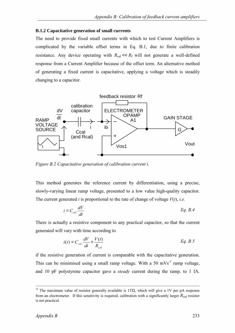
Appendix B: Calibration of feedback current amplifiers
Appendix B 233
B.1.2 Capacitative generation of small currents The need to provide fixed small currents with which to test Current Amplifiers is
complicated by the variable offset terms in Eq. B.1, due to finite calibration
resistance. Any device operating with Rcal << Rf will not generate a well-defined
response from a Current Amplifier because of the offset term. An alternative method
of generating a fixed current is capacitative, applying a voltage which is steadily
changing to a capacitor.
Rf
(and Rcal)
i ib
Vout
GAIN STAGE
G
A1
Vos1
VOLTAGESOURCE
ELECTROMETEROPAMP
feedback resistor
calibrationcapacitor
RAMP
Ccal
dVdt
Figure B.2 Capacitative generation of calibration current i.
This method generates the reference current by differentiation, using a precise,
slowly-varying linear ramp voltage, presented to a low value high-quality capacitor.
The current generated i is proportional to the rate of change of voltage V(t), i.e.
dtdVCi cal= Eq. B.4
There is actually a resistive component to any practical capacitor, so that the current
generated will vary with time according to
calcal R
tVdtdVCti )()( += Eq. B.5
if the resistive generation of current is comparable with the capacitative generation.
This can be minimised using a small ramp voltage. With a 50 mVs-1 ramp voltage,
and 10 pF polystyrene capacitor gave a steady current during the ramp, to 1 fA.
74 The maximum value of resistor generally available is 1TΩ, which will give a 1V per pA response from an electrometer. If this sensitivity is required, calibration with a significantly larger Rcal resistor is not practical.

Appendix B: Calibration of feedback current amplifiers
Appendix B 234
Consequently the resistive contribution to the current is small, and Rcal due to the
capacitor can therefore be estimated as ≥1 PΩ.
The properties and stability of the ramp generator become the important requirements
in the capacitive method, together with any AC response of the electrometer as the
source and feedback impedances which are significant. The source impedance at high
frequencies, Zcal however, will be substantially lower than Rcal75, and therefore this
approach is most ideally used with a 'slow' (low frequency) electrometer to minimise
any noise gain.
B.1.3 Practical implementation of capacitative technique A voltage ramp generator has been described for this application (Harrison and Aplin,
2000a), in which the rising and falling periods of the voltage ramp can be used to
generate symmetrical positive and negative calibration currents, Figure B.3. With a
suitable capacitor connected, it becomes a Current Reference, readily arranged to
generate ± 0.5 pA.
The reference current is generated by differentiation, using a slowly increasing and
decreasing linear ramp voltage, presented to a low value polystyrene capacitor. The
reference current is only available during the duration of the ramp, but symmetrical
bipolar currents can be derived alternately, from the rising and falling edges, allowing
two point calibration. Measurements need to be made a little after the ramp begins, to
avoid transients. The output current can be deduced to reasonable accuracy (~2%)
solely by using precision components, although the accuracy may be improved by
direct measurement of the current using a standardised electrometer.
The circuit operates in the following manner. A stabilised 5.00 V supply is generated
using voltage reference IC1, and a 2.50 V reference derived from it using equal
precision resistors and follower IC4b. A crystal oscillator (IC2) is used to generate a
stable and symmetrical 15.625 mHz square wave at the output of IC3. The MOSFET
output stage of IC3 was found to deliver this square wave with precise amplitudes to
within 1 mV of the 5.00 V supply and ground. The square wave is used as the input to
75 Zcal is the parallel combination of Rcal and Xcal, the capacitative reactance.

Appendix B: Calibration of feedback current amplifiers
Appendix B 235
an integrator based on C1 and IC4a, via R1, with the integrator centred at 2.50 V. If
IC4 is chosen to have a negligible input bias current, the 5.00 V square wave will
cause equal bipolar integrator input currents, and associated rising and falling voltage
ramps at IC4a output. The final output current is generated via the differentiator
comprising C2 (the calibration capacitor Ccal) and the input stage of the Current
Amplifier connected.
The reference current i is given by
11
22 R
VCC
dtdVCi ∆== Eq. B.6,
where ∆V is the integrator input voltage (±2.50 V). C1, C2 and R1 are thermally
stable, close-tolerance components. The choice of C2 is based on a compromise
between a sufficiently large value to minimise the effect of unknown stray
capacitances (with the associated thermal and temporal stability of the connection
geometry) and a small value to maximise the source impedance and reduce the noise
gain of the electrometer at high frequencies. In practise the first constraint was found
to be the more important parameter, as the noise generated on the ramp voltage was
small and the electrometer could be operated in a low frequency mode.
The integrator can be reset using the MOSFET switches in IC5, which are set by
default in the RUN (i.e. current reference operating) condition. In the STOP state the
oscillator and counters are reset, and the output of IC4 is pulled to ground via IC5c.
This effectively eliminates leakage across the output capacitor C2 in the STOP state,
allowing the Current Reference to be permanently connected to a slow response
Current Amplifier, without any additional high impedance switching.
For the component values used, the rate of change of ramp voltage was measured
using a chart recorder to be ±52.5 mVs-1, with the ramp starting and finishing at
2.5 V. Tests using a Keithley 6512 electrometer showed the output current to be of
magnitude 470 ± 2 fA, alternately positive and negative for 32 s each. Measurements
were made 5 s after the ramp transition. The Current Reference was found to be stable
to ± 2 fA for slowly-varying temperatures over the range −22 to 21.7 °C. The bipolar
output currents also remained symmetrical to within the accuracy of measurement

Appendix B: Calibration of feedback current amplifiers
Appendix B 236
over this range, although sudden thermal shocks to the output capacitor C2 during
initial cooling led to some transient asymmetric currents.

Appendix B: Calibration of feedback current amplifiers
Appendix B 237
Figure B.3 Schematic of the 500 fA Current Reference circuit. IC1 REF50Z 5 V
±30ppm/°C voltage reference; IC2 4060 oscillator divider; IC3 4040 binary divider;
IC4 LTC1047 chopper stabilised dual opamp; IC5 4066 quad MOSFET switch; R1
10 MΩ ±1% ±50ppm/°C metal film; C1 4.7 µF ±1% polyester layer ±200ppm/°C; C2
10 pF polystyrene ±80ppm/°C; X 32768 Hz quartz crystal.

Appendix C: Program source code
Appendix C 238
Appendix C
Program source code Listings for the most important microcontroller programs are given below. They are
written in PBASIC (Parallax, 1998), which is a variant of BASIC with extra
commands to control the microcontroller (e.g. setting the I/O pin states).
Source code for a program written in Turbo Pascal, DECINT, which performed the
decay integral in Chapter 8 is also given. C.1 Chapter 4 The program GNOCLOCK interfaces a 12-bit A to D converter, and switches
between two critical mobilities using reed relays to change the bias voltage. ‘GNOCLOCK.BAS‘Karen Aplin 02/02/99dirs=%01100000 ' makes pins 5 and 6 (connected to
relays)outputssymbol CS = 2 ' ADC Chip select (Low True)symbol CLK = 3 ' ADC Clocksymbol Din = pin4 ' Data input pin numbersymbol DatIn = 4 ‘ ADC Data Inputsymbol Dout = pin4 ' Data output pin numbersymbol DatOut= 4 ' ADC Data Outputsymbol ADbits= b1 ' Loop counter used to receive bitssymbol ADRes = w1 ' 12-bit ADC conversion resultsymbol sglDif= 1 ' 1 -> Single-ended, two-channel mode.symbol msbf = 1 ' Output 0s after data transfer is
completesymbol oddSign = bit0 ' Channel number
Init:high CS ' Deactivate the ADC to begin.
switch: ' Main part of programserout 1,N300,(90) ' outputs "Z" to PC serially toidentify serout 1,N300,(10) modeserout 1,N300,(13)pin5=1pin6=1 ' Both relays on (shorts out Rf to
prevent transients)pause 10000 ' waits for 10sgosub logserout 1,N300,(95) ' outputs "-" to PC seriallyserout 1,N300,(10)serout 1,N300,(13)pins=0 ' Both relays off – switches on
negative Vb and turns off shortingrelay

Appendix C: Program source code
Appendix C 239
pause 120000 ' waits for 2 mingosub log ' reading 1pause 6000 ' waits for 1 sgosub log ' reading 2pause 6000 ' waits for 1 sgosub log ' reading 3pause 6000 ' waits for 1 sgosub log ' reading 4pause 6000 ' waits for 1 sgosub log ' reading 5pause 6000 ' waits for 1 sgosub log ' reading 6serout 1,N300,(43) ‘ outputs "+" to PCserout 1,N300,(10)serout 1,N300,(13)pin6=0pin5=1 ' Switches on positive Vbpause 1800000 ' waits for 3 mingosub log ' reading 1pause 6000 ' waits for 1 sgosub log ' reading 2pause 6000 ' waits for 1 sgosub log ' reading 3pause 6000 ' waits for 1 sgosub log ' reading 4pause 6000 ' waits for 1 sgosub log ' reading 5pause 6000 ' waits for 1 sgosub log ' reading 6goto switch ' repeats whole process forever
'*******************************************************************log: ' logging subroutine
oddSign = 0gosub Convertserout 1,N300,(#ADRes) ' outputs ADC reading to PCserout 1,N300,(10)serout 1,N300,(13)return ' returns to switching loop
Convert: ‘ ADC Converter subroutinelow CLK ' Low clock--output on rising edge.high DatOut ' Switch DIO to output high (start
bit).low CS ' Activate the 1298.pulsout CLK,5 ' Send start bit.let Dout = sglDif ' First setup bit.pulsout CLK,5 ' Send bit.let Dout = oddSignpulsout CLK,5 ' Send bit.let pin4 = msbf ' Final setup bit.(total 3 bit input)pulsout CLK,5 ' Send bit.input DatInlet ADRes = 0 ' Clear old ADC result.for ADbits = 1 to 13 ' Get null bit + 12 data bits.let ADRes = ADRes*2+Din ' Shift AD left, add new data bit.pulsout CLK,5 ' Clock next data bit in.next ' Get next data bit.high CS ' Turn off the ADCreturn ' Return to program.

Appendix C: Program source code
Appendix C 240
C.2 Chapter 5 This section contains the programs developed to control the PIMS system. Section
C.2.1 gives the routine written to control the DAC, and the remainder of the programs
control the multimode electrometer. The programs used separately to test the modes
are given first, and followed by MMESYS, the overall PIMS control program. The
MME switching logic is given in Appendix A.
C.2.1 DAC driver The DAC driver routine was written by J.R. Knight. It stores the DAC voltage codes
in the microcontroller memory, and after the DAC is initialised, it reads through the
binary DAC code to send it bit by bit to the DAC. ‘JRK2.BAS'DAC driver routine JRK 25/05/99 simple-data versiondirs=%11111111 ' makes all pins outputssymbol CSDAC = 0 ' DAC Chip Selectsymbol CLK = 3 ' ADC/DAC Clocksymbol Din = pin4symbol stp = b2symbol stp2 = b3symbol data = b4symbol tem = b5symbol mask = b6symbol vsteps = 2 ' (number of voltage steps – 1)
read 255,data ' reads out eeprom space availabledebug data
init: eeprom 0,(0,128,255) ' stores voltage codes in EEPROMhigh csdaclow clk
loop: ‘ main part of DAC driverfor stp = 0 to vsteps ‘ steps through sequence of voltage
codeslow csdacdata = 9 ' control byte needed to initialise DACgosub sendread stp,data ‘ Reads voltage code into memorydebug datagosub sendhigh csdac
pause 5000' Additional functions of the programcan be added here.
nextgoto loop ‘ Starts sequence again

Appendix C: Program source code
Appendix C 241
send: ‘ Produces a control byte to send toDAC
mask=128for stp2= 0 to 7 ‘ Loop which moves along the bits in
the control byte one by onetem=mask & datadin=0if tem=0 then pulsedin=1
pulse: ‘ Sends 1 digital pulse to DACpulsout CLK,500
mask=mask/2 ‘ Moves one step along the binarysequence to be sent to DAC
nextreturn ‘ Returns to program
C.2.2 MME test programs IBLOG switches the MME into leakage check mode and input offset voltage
measurement mode. It then logs the output serially. ' error check mode logging program (IBLOG.BAS)' Karen Aplin 25/01/00dirs=%11110111 'makes all pins except 4 outputssymbol CE = pin7 'MME logic control linessymbol CY = pin5symbol CX = pin6symbol CSADC = 2 ' ADC Chip select (Low True)symbol CLK = 3 ' ADC/DAC Clocksymbol Din = pin4symbol Dout = pin4symbol Dpin = 4symbol ADRes = w1 ' 12-bit ADC conversion resultsymbol sglDif= 0 ‘ ADC in differential modesymbol msbf = 1symbol oddSign= 0symbol ADBits = b4symbol hh = b8 ' variable controlling number ofsamples
main: ‘ main part of program – steps througherror check modes
gosub ibgosub loggosub Vosgosub loggoto main
ib: ‘ MME leakage current modeCE = 0 ‘ Logic control to select modeCY = 1CX = 1serout 1,N300,("ib",44) ‘ Sends character to denote mode to
logging PC seriallypause 1000return

Appendix C: Program source code
Appendix C 242
Vos: ‘ MME input offset voltage modeCE = 0CY = 1CX = 0serout 1,N300,("Vos",44)pause 1000return
log: for hh = 1 to 29 ' logging looppause 5000 ' pause length determines sampling
frequencygosub convertserout 1,N300,(#ADRes,44)' output reading to PCnextpause 5000 ' recovery time before last readinggosub convertserout 1,N300,(#ADRes,13,10)'last reading with carriage returnreturn
convert: ‘ ADC Driverlow CLK ' Low clock--output on rising edge.high Dpin ' Switch DIO to output high (start
bit).low CSADC ' Activate the 1298.pulsout CLK,5 ' Send start bit.let Dout = sglDif ' First setup bit.pulsout CLK,5 ' Send bit.let Dout = oddSignpulsout CLK,5 ' Send bit.let Dout = msbf ' Final setup bit.(total 3 bit input)pulsout CLK,5 ' Send bit.input Dpinlet ADRes = 0 ' Clear old ADC result.for ADbits = 1 to 13 ' Get null bit + 12 data bits.let ADRes = ADRes*2+Din ' Shift AD left, add new data bit.pulsout CLK,50 ' Clock next data bit in.next ' Get next data bit.high CSADC ' Turn off the ADCoutput Dpin ' makes D output againreturn ' Return to program.
ICAL sets the MME into current measurement mode and calculates average currents
which are sent to the PC serially. It is designed to calibrate the MME picoammeter
function with the femtoampere current reference reference (Harrison and Aplin,
2000a).
' ical.BAS' Karen Aplin 25/01/00dirs=%11110111 'makes all pins except 4 outputssymbol CE = pin7 'MME logic controlsymbol CY = pin5symbol CX = pin6symbol CSADC = 2 ' ADC Chip select (Low True)symbol CLK = 3 ' ADC/DAC Clocksymbol Din = pin4

Appendix C: Program source code
Appendix C 243
symbol Dout = pin4symbol Dpin = 4symbol Datasum = w3 'Word variable storing the sum ofsamples
to averagesymbol ADRes = w1 ' 12-bit ADC conversion resultsymbol sglDif= 0 ' ADC in differential modesymbol msbf = 1symbol oddSign = 0symbol ADBits = b4symbol hh = b8 ' no of samples to average oversymbol CSDAC = 0 ' DAC Chip Selectsymbol stp = b2symbol stp2 = b3symbol data = b4symbol tem = b5symbol mask = b6symbol vsteps = 2 ' (voltage steps) - 1
CE = 0 ' sets MME into picoammeter modeCX = 1CY = 0
main: gosub log ' main loopgoto main
log:Datasum = 0 ' Resets sum of samples to zerofor hh = 1 to 5 ' Number of points to average overgosub convertDatasum = Datasum + Adres ' Adds the instantaneous reading to
thetotal
pause 1000 ' sampling frequency (1000 = 1 s)debug DatasumnextDatasum=Datasum/5 ' calculates the average valuedebug "mean",#Datasum ' shows mean on screenserout 1,N300,(#Datasum)' outputs reading serially to PCreturn
convert: ' ADC driverlow CLK ' Low clock--output on rising edge.high Dpin ' Switch DIO to output high (start
bit).low CSADC ' Activate the 1298.pulsout CLK,5 ' Send start bit.let Dout = sglDif ' First setup bit.pulsout CLK,5 ' Send bit.let Dout = oddSignpulsout CLK,5 ' Send bit.let Dout = msbf ' Final setup bit.(total 3 bit input)pulsout CLK,5 ' Send bit.input Dpinlet ADRes = 0 ' Clear old ADC result.for ADbits = 1 to 13 ' Get null bit + 12 data bits.let ADRes = ADRes*2+Din ' Shift AD left, add new data bit.pulsout CLK,50 ' Clock next data bit in.next ' Get next data bit.high CSADC ' Turn off the ADCoutput Dpin ' makes D output again

Appendix C: Program source code
Appendix C 244
return ' Return to program.
DECAY tests the MME follower mode, and the voltage decay of the central electrode.
It charges up the central electrode, switches it off and makes 2 Hz measurements of
the voltage decay in follower mode. The bias voltage can also be varied cyclically.
' Multimode electrometer decay mode test program (decay.BAS)' Karen Aplin 15/02/00dirs=%11110101 ' makes pins 0,2,4-7 outputssymbol CSADC = 2 ' ADC Chip select (Low True)symbol CLK = 3 ' ADC/DAC Clocksymbol Din = pin4symbol Dout = pin4symbol Dpin = 4symbol data = b0symbol ADRes = w1 ' 12-bit ADC conversion resultsymbol sglDif = 0symbol msbf = 1symbol oddSign = 0symbol ADBits = b4symbol hh = b8symbol CE = pin7 ' MME logicsymbol CY = pin5symbol CX = pin6symbol ADComp = w5symbol CSDAC = 0 ' DAC Chip Selectsymbol stp = b2 ' DAC controller variablessymbol stp2 = b3symbol tem = b5symbol mask = b6
let stp = 1eeprom 0,(0,0,0) ' stores voltage codeshigh csdac
low clklow csdacdata = 9 'control bytegosub sendread stp,datadebug datagosub sendhigh csdac
main: ' main part of programCE = 1 ' MME logic to charge up central
electrodeCY = 0CX = 0debug "Charged",cr ' screen messagepause 100CE = 0 ' switches off central electrode
voltage and puts MME into follower modepause 100serout 1,N300,(10,13) ' starts new line in logging filefor hh = 1 to 30 ' defines how many points to be
measured in decay
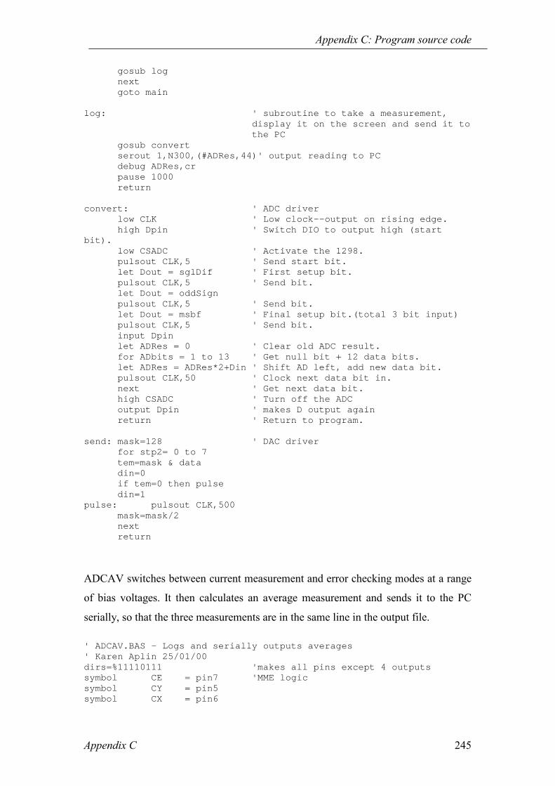
Appendix C: Program source code
Appendix C 245
gosub lognextgoto main
log: ' subroutine to take a measurement,display it on the screen and send it tothe PC
gosub convertserout 1,N300,(#ADRes,44)' output reading to PCdebug ADRes,crpause 1000return
convert: ' ADC driverlow CLK ' Low clock--output on rising edge.high Dpin ' Switch DIO to output high (start
bit).low CSADC ' Activate the 1298.pulsout CLK,5 ' Send start bit.let Dout = sglDif ' First setup bit.pulsout CLK,5 ' Send bit.let Dout = oddSignpulsout CLK,5 ' Send bit.let Dout = msbf ' Final setup bit.(total 3 bit input)pulsout CLK,5 ' Send bit.input Dpinlet ADRes = 0 ' Clear old ADC result.for ADbits = 1 to 13 ' Get null bit + 12 data bits.let ADRes = ADRes*2+Din ' Shift AD left, add new data bit.pulsout CLK,50 ' Clock next data bit in.next ' Get next data bit.high CSADC ' Turn off the ADCoutput Dpin ' makes D output againreturn ' Return to program.
send: mask=128 ' DAC driverfor stp2= 0 to 7tem=mask & datadin=0if tem=0 then pulsedin=1
pulse: pulsout CLK,500mask=mask/2nextreturn
ADCAV switches between current measurement and error checking modes at a range
of bias voltages. It then calculates an average measurement and sends it to the PC
serially, so that the three measurements are in the same line in the output file. ' ADCAV.BAS - Logs and serially outputs averages' Karen Aplin 25/01/00dirs=%11110111 'makes all pins except 4 outputssymbol CE = pin7 'MME logicsymbol CY = pin5symbol CX = pin6

Appendix C: Program source code
Appendix C 246
symbol CSADC = 2 ' ADC Chip select (Low True)symbol CLK = 3 ' ADC/DAC Clocksymbol Din = pin4symbol Dout = pin4symbol Dpin = 4symbol Datasum = w3symbol ADRes = w1 ' 12-bit ADC conversion resultsymbol sglDif= 0 ' ADC in differential modesymbol msbf = 1symbol oddSign= 0symbol ADBits = b4symbol hh = b8 ' used in loop: no of points to average
oversymbol CSDAC = 0 ' DAC Chip Selectsymbol CLK = 3 ' ADC/DAC Clocksymbol Din = pin4symbol stp = b2symbol stp2 = b3symbol data = b4symbol tem = b5symbol mask = b6symbol vsteps = 2 'voltage steps minus one
main: ‘ main loopeeprom 0,(0,128,255) ' reads voltage codes into memoryfor stp = 0 to vstepslow csdacdata = 9 ' DAC control bytegosub sendread stp,datadebug datagosub sendhigh csdaclow clkgosub ib ‘ leakage check modegosub log ‘ logs datagosub Vos ‘ input offset voltage check modegosub loggosub current ‘ current measurement modegosub loggoto main
ib:CE = 0 ‘ switches MME to leakage check modeCY = 1CX = 1debug "ib"serout 1,N300,(44) ‘ sends comma to PC logging filepause 10000 ‘ 10s recovery time from transientreturn
Vos:CE = 0CY = 1CX = 0debug "Vos"serout 1,N300,(44)pause 10000return
current:

Appendix C: Program source code
Appendix C 247
CE = 0CX = 1CY = 0debug "current"serout 1,N300,(10,13) ‘ sends carriage return and line feed
to PC logging filepause 10000return
log: ‘ averaging/logging routineDatasum = 0for hh = 1 to 10gosub convertDatasum = Datasum + ADrespause 1000debug DatasumnextDatasum=Datasum/10debug "mean",#Datasumserout 1,N300,(#Datasum)' output reading to PCreturn
convert: ‘ ADC driverlow CLK ' Low clock--output on rising edge.high Dpin ' Switch DIO to output high (start
bit).low CSADC ' Activate the 1298.pulsout CLK,5 ' Send start bit.let Dout = sglDif ' First setup bit.pulsout CLK,5 ' Send bit.let Dout = oddSignpulsout CLK,5 ' Send bit.let Dout = msbf ' Final setup bit.(total 3 bit input)pulsout CLK,5 ' Send bit.input Dpinlet ADRes = 0 ' Clear old ADC result.for ADbits = 1 to 13 ' Get null bit + 12 data bits.let ADRes = ADRes*2+Din ' Shift AD left, add new data bit.pulsout CLK,50 ' Clock next data bit in.next ' Get next data bit.high CSADC ' Turn off the ADCoutput Dpin ' makes D output againreturn ' Return to program.
send: mask=128 ‘ DAC driverfor stp2= 0 to 7tem=mask & datadin=0if tem=0 then pulsedin=1
pulse: pulsout CLK,500mask=mask/2nextreturn
MMESYS is the final program used to operate the PIMS in all its modes (as given in
Table A.1), and take measurements of voltage decays and current samples.
MMESYS2 is shown here; the only difference between the programs for the different
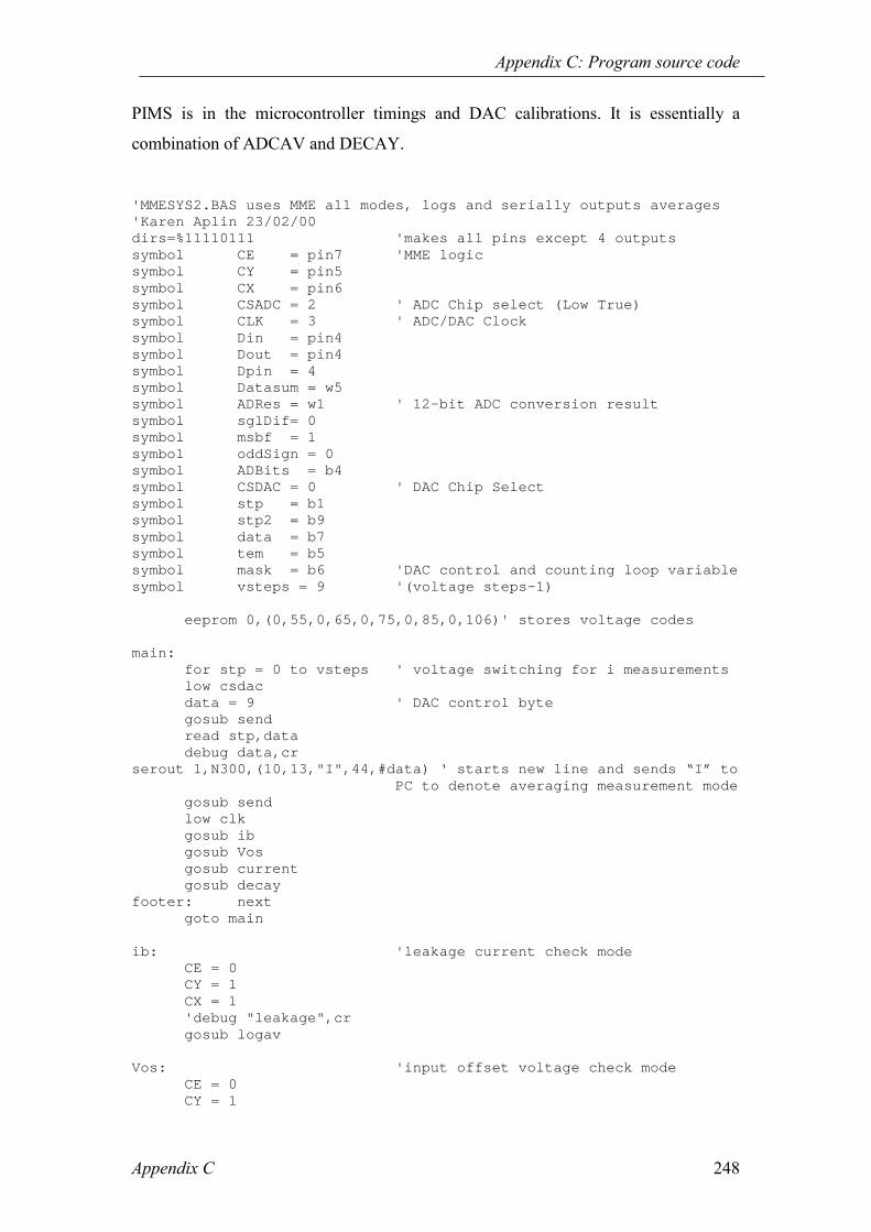
Appendix C: Program source code
Appendix C 248
PIMS is in the microcontroller timings and DAC calibrations. It is essentially a
combination of ADCAV and DECAY.
'MMESYS2.BAS uses MME all modes, logs and serially outputs averages'Karen Aplin 23/02/00dirs=%11110111 'makes all pins except 4 outputssymbol CE = pin7 'MME logicsymbol CY = pin5symbol CX = pin6symbol CSADC = 2 ' ADC Chip select (Low True)symbol CLK = 3 ' ADC/DAC Clocksymbol Din = pin4symbol Dout = pin4symbol Dpin = 4symbol Datasum = w5symbol ADRes = w1 ' 12-bit ADC conversion resultsymbol sglDif= 0symbol msbf = 1symbol oddSign = 0symbol ADBits = b4symbol CSDAC = 0 ' DAC Chip Selectsymbol stp = b1symbol stp2 = b9symbol data = b7symbol tem = b5symbol mask = b6 'DAC control and counting loop variablesymbol vsteps = 9 '(voltage steps-1)
eeprom 0,(0,55,0,65,0,75,0,85,0,106)' stores voltage codes
main:for stp = 0 to vsteps ' voltage switching for i measurementslow csdacdata = 9 ' DAC control bytegosub sendread stp,datadebug data,cr
serout 1,N300,(10,13,"I",44,#data) ‘ starts new line and sends “I” toPC to denote averaging measurement mode
gosub sendlow clkgosub ibgosub Vosgosub currentgosub decay
footer: nextgoto main
ib: 'leakage current check modeCE = 0CY = 1CX = 1'debug "leakage",crgosub logav
Vos: 'input offset voltage check modeCE = 0CY = 1
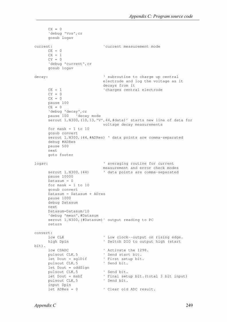
Appendix C: Program source code
Appendix C 249
CX = 0'debug "Vos",crgosub logav
current: 'current measurement modeCE = 0CX = 1CY = 0'debug "current",crgosub logav
decay: ‘ subroutine to charge up centralelectrode and log the voltage as itdecays from it
CE = 1 'charges central electrodeCY = 0CX = 0pause 100CE = 0'debug "decay",crpause 100 'decay modeserout 1,N300,(10,13,"V",44,#data)’ starts new line of data for
voltage decay measurementsfor mask = 1 to 10gosub convertserout 1,N300,(44,#ADRes) ‘ data points are comma-separateddebug #ADRespause 500nextgoto footer
logav: ‘ averaging routine for currentmeasurement and error check modes
serout 1,N300,(44) ‘ data points are comma-separatedpause 10000Datasum = 0for mask = 1 to 10gosub convertDatasum = Datasum + ADrespause 1000debug DatasumnextDatasum=Datasum/10'debug "mean",#Datasumserout 1,N300,(#Datasum)' output reading to PCreturn
convert:low CLK ' Low clock--output on rising edge.high Dpin ' Switch DIO to output high (start
bit).low CSADC ' Activate the 1298.pulsout CLK,5 ' Send start bit.let Dout = sglDif ' First setup bit.pulsout CLK,5 ' Send bit.let Dout = oddSignpulsout CLK,5 ' Send bit.let Dout = msbf ' Final setup bit.(total 3 bit input)pulsout CLK,5 ' Send bit.input Dpinlet ADRes = 0 ' Clear old ADC result.

Appendix C: Program source code
Appendix C 250
for ADbits = 1 to 13 ' Get null bit + 12 data bits.let ADRes = ADRes*2+Din ' Shift AD left, add new data bit.pulsout CLK,50 ' Clock next data bit in.next ' Get next data bit.high CSADC ' Turn off the ADCoutput Dpin ' makes D output againreturn ' Return to program.
send: ‘ DAC drivermask=128for stp2= 0 to 7tem=mask & datadin=0if tem=0 then pulsedin=1
pulse: pulsout CLK,500mask=mask/2nextreturn
C.3 Chapter 8 DECINT was written by R.G. Harrison and performs the numerical integration to
simulate a voltage decay with a predefined spectrum.
Program DECINT; DECayINTegral program to perform numerical integrations to calculate the decayof voltage across electrodes of Gerdien tube(1) in the simplest case (single ion mobility) this is an
exponential(2) with an ion mobility spectrum, the decay deviates from an
exponentialwhich is found by integrating over the mobility spectrum up to the
criticalmobility determined by the instantaneous voltage generated from the
decay(3) mobility spectrum is assumed to be Gaussian (fitting Estonian
data)(4)integration performed using quality-controlled Simpson's rule
Giles Harrison March 2000
type integer=longint;
consttube parametersa=11.0; mmb=2.0; mmL=0.25; mu=2.0; m.s-1epsilon = 8.841941e-12; permittivity of free space [Farads per
metre]Qe =1.6021892e-19; modulus of electronic charge
[Coulombs]
vartimesum,V0,VT,V1,V2,T12,upperMu,lowerMu,MobInt,VoltInt,IonSum:real;TrapzdIt: integer;

Appendix C: Program source code
Appendix C 251
Npoints,i:integer;fout:text;
1. function to compute critical mobility from tube parameters, as afunction of the applied bias voltage Vfunction MuCrit(V:real):real; in cm2.v-1.s-1beginMuCrit:= ((sqr(a)-sqr(b))*1.0e-6*ln(a/b) * u)/(2.0*V*L)/1.0e-4;end;
2. Integrand for ion mobility spectrum, generated by Gaussian fit toEstonian data
FUNCTION func1(X:EXTENDED):EXTENDED;consta=130.22902;b=1.4791917;c=0.39179526;vary:real;BEGIN integral for (positive) ion spectrum
fitted to Gaussian curvey:=100.0* to convert cm-based units to SI
10.0*a * exp( -sqr(x-b)/ (2.0*sqr(c) ) );func1:= y;
END;
implementation of Simpson's rule, as coded in "Numerical Recipes inPascal"which calls the Trapezium rule first
PROCEDURE trapzd1(a,b: real;VAR s: real;
n: integer);VAR
j: integer;x,tnm,sum,del: real;
BEGINIF n = 1 THEN BEGIN
s := 0.5*(b-a)*(func1(a)+func1(b));TrapzdIt := 1
ENDELSE BEGIN
tnm := TrapzdIt;del := (b-a)/tnm;x := a+0.5*del;sum := 0.0;FOR j := 1 TO TrapzdIt DO BEGIN
sum := sum+func1(x);x := x+del
END;s := 0.5*(s+(b-a)*sum/tnm);TrapzdIt := 2*TrapzdIt
ENDEND;
PROCEDURE qsimp1(a,b: real;VAR s: real);
LABEL 99;CONST
eps = 1.0e-3;

Appendix C: Program source code
Appendix C 252
jmax = 20;VAR
j: integer;st,ost,os: real;
BEGINost := -1.0e30;os := -1.0e30;FOR j := 1 TO jmax DO BEGIN
trapzd1(a,b,st,j);s := (4.0*st-ost)/3.0;IF abs(s-os) < eps*abs(os) THEN GOTO 99;os := s;ost := st
END;writeln ('pause in QSIMP1- too many steps');readln;
99:END;
3. find time taken for the voltage decay (which requires theintegration overthe mobility spectrum up to the critical mobility at each voltage) function decaytime(V0,VT:real):real;beginupperMu:=MuCrit(VT);lowerMu:=MuCrit(V0);writeln(lowerMu,' ', upperMu);qsimp1(lowerMu,upperMu,MobInt); mobility spectrumVoltInt:=ln(VT/V0);decaytime:=-(epsilon/Qe)* (VoltInt/MobInt) ;end;
BEGIN main program
open output file file, comma-separated for Excelassign(fout,'c:\temp\decay.csv');rewrite(fout);writeln(fout,'volts,timediff,time');
compute time taken T12 for decay from V1 to V2 ultimately, byevaluating thedecay integral from V1 down to VT over ion mobility spectrum-evaluated at 10 points in the decayV1:=10; V2:=1;Npoints:=10;writeln(V1:3:2,',0');writeln(fout,V1:3:2,',0');timesum:=0;for i:=Npoints downto 1 do
beginVT:=i*( (V1-V2)/Npoints);V0:=((i+1)*(V1-V2))/Npoints;
writeln(V0:3:2,' ',VT:3:2);T12:=decaytime(V0,VT);timesum:=timesum+T12;writeln(VT:3:2,',',T12:16,',',timesum:16);writeln(fout,VT:3:2,',',T12:16,',',timesum:16);end;

Appendix C: Program source code
Appendix C 253
close(fout); close output fileEND.

Appendix D: Engineering Diagrams
Appendix D 254
Appendix D
Gerdien Engineering Diagrams
This appendix contains the engineering diagrams for the new design of stainless steel
Gerdien described in Chapter 5. The Gerdien and diagrams were designed and
prepared by S. D. Gill and A.G. Lomas. The diagrams are supplied in a folder in the
inside back cover of the Thesis. A summary of their content is given in Table D.1
below. (Figure 5.2 is a photograph of the Gerdien in construction.)
Drawing Title Description
Gerdien tube Outside of the tube showing BNCs and end
of central electrode
Gerdien tube assembly full detail As above but shows internal components as
dotted lines
Gerdien tube sectioned Shows two cross-sections of the tube
AA: longitudinal, showing central
electrode detail
BB: transect through central electrode
connector
Gerdien tube part sectioned As Gerdien tube but shows central
electrode inside the tube.
Gerdien tube components Shows individual components. Modified
and given in main text as Figure 5.1.

Appendix E: Historical discussion
Appendix E 255
Appendix E
The development of an integrated scientific perception of atmospheric particulates during the twentieth century E.1 Introduction Interest in the electrical properties of the air is not new and probably began as a result
of curiosity about spectacular natural phenomena like the aurorae and lightning. Yet
successful measurements and understanding of air-borne particles, which contribute to
these phenomena, are clearly products of the science of the twentieth century. The
reasons for the surge of interest in the field from 1898 onwards are examined and
suggest that a complex combination of scientific circumstances played a crucial rôle,
motivating and facilitating research into air ions and their electrical properties. The
development of the subject is followed, towards the modern approach of the present
day, with air ions generally considered as part of the continuum of atmospheric
aerosol particles. Finally, a case study of the relationship between atmospheric small
ion and aerosol concentration acts as a supporting example, and relates historical
scientific discoveries to contemporary work (e.g. Guo et al., 1996).
E.1.1 Air ions in context Today the study of air ions is based primarily upon the idea of their continual
interaction with other parts of the atmospheric aerosol spectrum, but their special
contribution to atmospheric electricity is also recognised. This article traces the rôle
of air ions and their relevance to different aspects of twentieth century physics, within
a broad historical context.
The route to our current perception of air ion behaviour can be characterised by the
development of two focal areas. Firstly, there was a need for a semantic framework to
describe and answer problems effectively. The unification of the initially separate
studies of dust and air ions was also a crucial step in the progression towards the
contemporary approach.

Appendix E: Historical discussion
Appendix E 256
E.1.2 Background: The discovery of the electron The first publication directly related to air ions seems to be by Zeleny in 1897 and
research into the subject became very popular in the early years of this century. In a
thorough and well-researched article, Flagan (1998) suggests that the problem of
charge dissipation in the atmosphere was enough to motivate the plethora of papers
published from 1898-1930. This problem had been known for many years, and could
ostensibly only be investigated after the discovery of the electron in 1897 by J.J.
Thomson explained the true nature of the ion. Yet it seems unlikely that this would be
a pressing enough problem for so many workers to become involved, especially when
there was so much new work to do in physics at the turn of the century. In addition,
much of the research into air ions clearly evolved from experiments initially unrelated
to atmospheric science, see for example Rutherford (1897) and McClelland (1898).
Ions were first identified by Faraday in his 19th century work on electrochemistry, and
were known to be produced by some sort of breakdown of molecules in an electric
field. Helmholtz developed this work to define the electric charge on the atom as the
finite quantity of electricity carried by all ions. Stoney then used the word electron
for the first time to describe a fundamental amount of electricity (Robotti, 1995). It is
well known that J.J. Thomson identified the constituents of cathode rays as the first
sub-atomic particles, which he called corpuscles, in 1897. As the idea of the atom
breaking up in any way had been inconceivable since Democritus, who first used the
term, Thomson lacked sufficient evidence to immediately identify the corpuscle with
a fundamental unit of both electricity and matter. Robotti discusses Thomsons
attempts to measure the charge of the corpuscles independently. It was only when this
measurement had been completed, that the corpuscle could be recognised as the
electron. According to Robotti, Thomson based the whole research programme at the
Cavendish Laboratory around this aim. It is fortunate for physics, and meteorology in
particular, that he did so. Ernest Rutherford and C.T.R. Wilson were taken on as
research students in the 1890s. Although they became famous for work outside this
field, (Wilsons being particularly important to meteorology) both men produced
valuable work related to ions in the air during this period at the Cavendish
Laboratory.

Appendix E: Historical discussion
Appendix E 257
One of the areas investigated by Thomson was the conduction of electricity through
gases. Coulomb in 1795 was the first person to notice that the atmosphere is slightly
electrically conductive, finding that an insulated gold leaf electrometer would
discharge slowly in air. Roentgens timely discovery of X-rays (in 1896) was another
circumstance that abetted research into ions in gases. It was quickly found that
Roentgen rays made gases electrically conductive by ionisation. This probably
appealed to Thomson because of the potential for measuring the charge of the
corpuscles that were produced. The Concise Dictionary of Scientific Biography76
(1981) explains that Thomson took a new approach to the problem of conduction of
electricity through gases, describing ions in terms of experimentally defined
parameters (such as mobility) when previously, only the dynamics of molecular
collisions were considered (proving inadequate to explain the problem). This could
well derive from his desire to measure the charge on the corpuscle without reference
to pre-existing particles. The arrival of the experimentalist C.T.R. Wilson at the
laboratory permitted further progress with some theoretical work of Thomsons from
1893, relating to the effect of charged particles on condensation. Roentgen rays were
found to increase the condensation rate in a saturated chamber, and these results,
combined with Thomsons relating to ionisation increasing the electrical conductivity
of gases, led them to surmise that ions acted as cloud condensation nucleii in
supersaturated conditions not found in the atmosphere (Robotti, 1995).
This work did not lead to the direct measurement of the charge of the corpuscle, but it
provided a method for e to be measured using the photoelectric effect. Thomson could
then present his revolutionary idea, that the electron was fundamental, both as a unit
of electrical charge and within the atom. Robotti summarises, Thomsons
measurement of the charge of the corpuscle meant that all electrical phenomena
would have to be re-examined. This is absolutely fundamental to the history of air
ion measurements. Thomsons preliminary work had provided a conceptual and
experimental framework within which atmospheric electricity could be considered,
and his eventual result provided motivation for further work in all aspects of
electricity.
76 Concise Dictionary of Scientific Biography (1981), Scribner

Appendix E: Historical discussion
Appendix E 258
E.2 Development of the study of air ions One way to define science is as a progressive activity which moves from one theory
to another (e.g. Kuhn, 1967), with later theories generally thought of as closer
approximations to the truth. One does not have to subscribe to any particular
philosophical approach to scientific progress to appreciate that every new framework
of scientific thought brings with it a new terminology. The acknowledgement and
ultimately, application of the new language by scientists working in similar fields
signifies the true acceptance of the exemplar. Thomsons work on gaseous ions was
hardly revolutionary on the same scale as the discovery of the electron, more a new
approach which had evolved from his efforts to solve a different problem. Yet it did
require a new terminology, and the development of the 20th century approach to ion
measurements can be traced by the introduction of Thomsons new terms into the
scientific vernacular.
Consider the concept of electrical mobility as defined by Thomson in his book The
Conduction of Electricity Through Gases, which was first published in 1903.
Evd=µ Eq. E.1
Mobility, µ, was a powerful parameter to describe the motion of ions in an electric
field because it relates the drift velocity attained by the charged particle, vd to E, the
magnitude of the electric field. This assumes the Stokes régime, which is when the
electrostatic forces acting on the particle balance the drag forces. After the work of
Wellisch (1909) and Cunningham (1910) electrical mobility could also be related to
particle radius and mass.
Zeleny (1898) discovered that negative ions needed a larger potential difference to be
deflected by the same amount as the positive ions. This implies that the negative ions
have a higher velocity (and hence mobility) than positive ions. Zeleny reported these
results apparently without appreciating the concept of mobility as defined by
Thomson. In his papers from 1898 and 1900, he refers continually to the velocity of
ions in an electrical field, and his tables of results are headed with, velocity of ions in
an electric field of 1 Vm-1. According to Flagan (1998), Zeleny was responsible for
the definition of critical mobility in the cylindrical condenser, that is, the minimum
mobility of ion that would hit the plate T and contribute to the electrometer deflection.

Appendix E: Historical discussion
Appendix E 259
With hindsight this is true, but Zeleny only defined a critical ionic velocity, indicating
that by 1900 the importance of mobility as a parameter had not been directly
recognised.
In 1900 C.T.R. Wilson described some experiments by Elster and Geitel related to the
rate of discharge of an electrified body in air. Using Thomsons value for the charge
on the ions, the ionisation rate was calculated at 20 ions cm-3s-1 for each sign.
Wilsons terminology in this paper is interesting. He was still working at the
Cavendish Laboratory at this time and had begun his scientific career under Thomson,
so Wilson, if anybody, would use the rhetoric developed by his supervisor. Yet he is
still referring to the charge on the ion, and not explicitly equating it to what is now
called the charge on the electron. However, as Thomson himself continued to refer to
the electron as the corpuscle occasionally until the 1920s, this is possibly
understandable. It appears that the concept of mobility was not outlined clearly until
Conduction of Electricity through Gases, which was published in 1903. This is
supported by the terminology used by Thomsons students; Rutherford (1897) only
refers to ionic velocity and not mobility. The concept of mobility (if not a full
understanding) seems to have been recognised by 1909, as Wellisch referred to it
continually in a paper entitled, On the mobilities of ions produced by Rontgen rays in
gases and vapours. Even though Wellisch first derived the relationship between
mobility µ and mass m,
m1∝µ Eq. E.2
he incorrectly used the units of velocity when referring to mobility. By 1914 Swann
was aware of the critical mobility of a cylindrical condenser, but still discussed
mobility indirectly, as a mass-velocity relationship. Pollack (1915) used the new term
explicitly when presenting results pointing to the existence of a larger, low mobility
ion in the air.
E.3 From “dust” to “aerosol” Aitken (1880) was one of the first scientists to study atmospheric aerosol, covering
many of the most important issues in aerosol science today in one short paper. He
suggested that infinitesimally small and invisible particles were necessary to create

Appendix E: Historical discussion
Appendix E 260
droplets in clouds, because burned sulphur had been shown to be a good fog
producer. Aitken also proposed the following sources of fine atmospheric dust: dried
spray from the ocean (salt was invoked separately), meteoric matter and combustion
products. In the 1890s Thomson and Wilson showed ions could also act as cloud
condensation nucleii. The first direct link between dust and ions is credited to
Rutherford (1897), who explained that dust particles reduced the conductivity of the
air because of the small ions attaching to them. In 1923 Nolan presented the results of
experiments showing that ions were surrounded by water molecules. This must have
provoked analogies between the smallest (ions) and largest particles (cloud droplets)
then known to exist in the atmosphere. Langevin (in Flagan, 1998) also furthered the
relationship between small ions and aerosol by discovering large ions. The large ion
concentration was found to correlate with the aerosol concentration, and was
anticorrelated with ionic variations, perhaps placing large ions between aerosol and
smaller ions in some broad spectrum. The third edition of Thomsons book (1928)
summarises contemporary work on ions in gases and their relationship to aerosol. He
interprets some very low mobility ions found by Langevin in Paris in 1908 as
charged particles of dust and relates them obliquely to pollution: the number of
them [is] much greater in large towns than in the open country.
The above summary of aerosol science in the first quarter of the century shows the
basis of the continuum view of atmospheric aerosol, and the growing perception of
aerosol as a product of anthropogenic activity. Yet nobody had directly referred to
particulates as pollutants. Aitken (1880) even suggested that sulphurs combustion
products might somehow deodorise Londons polluted streets. By the 1940s and
1950s scientists were becoming more aware of the magnitude and variety of
particulate matter emissions. The relevance and potential harmfulness of small
particles suspended in the air, which were becoming known as aerosol had also
been noted (Hewson, 1951). The emergence of this perception of aerosol pollution
was concurrent with the massive and uncontrolled growth of industrialisation and car
usage in the Western world (Elsom, 1992).
E.4 Small ions and particulate pollution A useful way to follow the progressive integration of initially discrete studies of

Appendix E: Historical discussion
Appendix E 261
small ions and atmospheric particulate matter is to consider the direct relationship
between them. The direct effect that particulates have on the air is to reduce its
electrical conductivity. The number of small ions, which cause the air to be slightly
conductive, decreases as the aerosol number concentration increases. This is because
of attachment of the ions to the much larger aerosol particles. This effect was first
noticed in the atmosphere by Wait (1946) following conductivity measurements over
the oceans on the cruises of the research ship Carnegie (Chalmers, 1967) from 1912
onwards. Rutherford (1897) had been the first to publish the idea that larger particles
reduce the number of small ions, but it took many years for this idea to be formalised
from its first inception (Rutherford, 1897). The relationship between aerosol
concentration and air conductivity has only recently been experimentally investigated
with the aim of improving aerosol measurements (Aplin et al., 1998). The progression
of separate measurements of air ions (e.g. Rutherford, 1897) and aerosol (Aitken,
1890) of the late 19th century towards their integration in the late 20th century (e.g.
Guo et al., 1996) is a useful indicator of the change in perceptions of atmospheric
particles.
Rutherfords initial attempts to describe ionic equilibrium in the air did not include
any effects from ions recombining with aerosol, although he clearly understood the
physical processes involved:
Since the dust-particles are very large compared with the ions, an ion is
more likely to strike against the dust-particle, and give up its charge to it or
to adhere to the surface and the rate of loss of conductivity is much more
rapid than if the loss of conductivity were due to collisions between the ions
themselves.
No attempt was made to express the attachment of small ions to larger particles
mathematically until Nolan et al. (1925). It is unclear why the Cambridge physicists
all neglected this effect in their equations, though they were well aware of it. (It is
possible that their outlook was so focussed upon investigating ions in the laboratory,
that they thought attachment to particles in the air was unimportant or unnecessary.)
In considering the equilibrium case, where the ion production rate equals the

Appendix E: Historical discussion
Appendix E 262
recombination rate, the only loss term expressed in the equation described self-
attachment (ions recombining with others of the opposite sign). The equation used by
Thomson, Rutherford and Wilson in many papers on this topic was:
2nq α= Eq. E.3
Here, q is the rate of ion production, n is the ion number concentration and α is an
self-attachment coefficient. Nolan et al. (1925) added an extra term to account for
ions combining with ions and larger particles. The rate of attachment is proportional
to the number of ions and the number of aerosol particles. The equation here is given
in the form used today (Nolan et al. used a slightly different notation).
nZnq βα += 2 Eq. E.4
In Eq. E.4, Z is the monodisperse aerosol number concentration and β is an
attachment coefficient. It took some time for this coefficient to be described
theoretically, possibly because of the complexity of the physics underlying the
attraction between a small charged particle and a larger uncharged one. Various
attempts were made to find β experimentally, but they varied over an order of
magnitude (Wait and Parkinson, 1951). β is dependent on the size of the ions and
aerosol particles measured, so further measurements made in different locations and
using different techniques added to the confusion. Bricard (1949) appears to have
developed the first working method for calculating β. After Bricard, a number of
other workers approached the problem; some of this is reviewed in Harrison (1992).
Acceptance of the idea of using the properties of the smallest particles in the air to
monitor the largest ones appears to have required the simultaneous development of
three branches of this field. Air conductivity measurements had to be carried out in a
variety of locations before it was realised that the urban areas showed much lower
conductivity than the rural ones. Long term clean air measurements of atmospheric
electrical parameters in the remote oceans led to the perception that clean air
conductivity could be used as a secular pollution indicator (Wait, 1946). An
awareness of increasing particulate pollution levels, combined with a rigorous
approach to aerosol attachment processes completed the knowledge needed to bring
the relationship between atmospheric electrical processes and aerosol to the state they
are in today.

Appendix E: Historical discussion
Appendix E 263
E.5 Conclusions There has been a kind of paradigm shift (Kuhn, 1967) in the science of atmospheric
particles during the twentieth century. Aitken started to investigate aerosol particles in
the 1880s, but understanding of the smallest particles lacked motivation or a
theoretical basis. Discovery of the electron provided justification for the existence of
the atmospheric ion, plus terminological and experimental frameworks to understand
the ions and their properties. Following this, measurements of air ions combined with
an increase in pollution necessitated development of theories explaining the
interaction of these particles. This established the methodology for the integrated way
scientists have studied atmospheric particulates in the second half of this century.
Without the progression elucidated above, there would not be the understanding of the
atmospheric aerosol continuum and its contemporary relevance for climate change,
pollution issues and atmospheric electricity.

References
References 264
References
Adachi M., Ishida T., Kim T.O., Okuyama K. (1996), Experimental evaluation of ion-
induced nucleation in nanometre-aerosol formation by α-radiolysis of SO2/H2O/N2
mixtures, Colloids and Surfaces A 109, 39-48
Aitken J. (1880), On dust, fogs and clouds, Nature, 22, 195
Aitken J., (1890), On the number of dust particles in the atmosphere, Trans. Roy. Soc.
Edin., 35, 1-19
Anderson R. V. and Bailey J.C. (1991), Errors in the Gerdien measurement of
atmospheric electrical conductivity, Meteorol. Atm. Phys, 46, 101-112
Aplin K.L. and Harrison R.G. (1999), The interaction between air ions and aerosol
particles in the atmosphere, In: Taylor D.M. (ed.), Proceedings of 10th International
Electrostatics Conference, Cambridge, 28th-31st March 1999, Institute of Physics
Conference Series 163, 411-414
Aplin K.L. and Harrison R.G. (2000), A computer-controlled Gerdien atmospheric
ion counter, Rev. Sci. Instrum., 71, 8, 3037-3041
Aplin K.L., Harrison R.G. and Wilkinson S. (1998), An electrical method of urban
pollution measurement, J. Aerosol Sci., 29, S1, 869-870
Arathoon J. (1991), Atmospheric Electricity Investigations: the Measurement of
Atmospheric Conductivity, BSc. Dissertation, University of Lancaster
Atkins P.W. (1989), Physical Chemistry, 4th edition, Oxford University Press
Bailey J.C., Blakeslee R.J., and Driscoll K.T. (1999), Evidence for the absence of
conductivity variations above thunderstorms, In: Christian H.J. (ed.), Proceedings
11th International Conference on Atmospheric Electricity, Guntersville, Alabama 7th-
11th June 1999 (NASA/CP-1999-209261), 646-649
Barlow J.F. (2000), Turbulent transfer of space charge in the atmospheric surface
layer, PhD Thesis, University of Reading.
Berthouex, P.M. and Brown, L.C. (1994), Statistics for Environmental Engineers,
CRC Press, Boca Raton

References
References 265
Blakeslee R.J. (1984), The electric current densities beneath thunderstorms, PhD
Thesis, University of Arizona
Blakeslee R.J. and Krider E.P. (1992), Ground level measurements of air
conductivities under Florida thunderstorms, J. Geophys. Res., 97, D12, 12947-12951
Bleaney B.I. and Bleaney, B. (1985), Electricity and magnetism, 3rd edition, Oxford
University Press
Bricard P.J. (1949), L'equilibre ionique de la basse atmosphere, J. Geophys. Res., 54,
39-52
Bricard J., Billard F. and Madelaine G. (1968), Formation and evolution of nuclei of
condensation that appear in air initially free of aerosols, J.Geophys Res 73, 14, 4487-
4496
Brownlee J.N. (1973), A fast mobility spectrometer for atmospheric ions, PhD Thesis,
University of Auckland
Brownlee J.N. (1975a), A new approach to atmospheric-ion mobility spectrometry, J.
Terr. Atm. Phys, 37, 1139-1144
Brownlee J.N. (1975b), Some measurements of atmospheric ion mobility spectra and
conductivity at Auckland, J. Terr. Atm. Phys, 37, 1145-1149
Castleman A.G. (1982), In: Schryer D.R., Heterogeneous atmospheric chemistry,
AGU, Washington
Chalmers J.A. (1967), Atmospheric Electricity, 2nd edition, Pergamon Press, Oxford
Clement C.F. and Harrison R.G. (1992), The charging of radioactive aerosols, J.
Aerosol Sci 23, 5, 481-504
Coulomb C.A. (1795), Premier mémoire sur lelectricité et le magnetisme, Histoire de
lAcadémie Royale des Sciences, Paris
Crozier W.D. (1964), The electric field of a New Mexico dust devil, J. Geophys Res.,
69, 5427-5429
Cunningham E. (1910), On the velocity of steady fall of spherical particles through
fluid medium, Proc. Roy. Soc. A., 83, 357-365

References
References 266
Dhanorkar S. and Kamra A.K. (1992), Relation between electrical conductivity and
presence of intermediate and large ions in the lower atmosphere, J. Geophys. Res., 97,
20345-20360
Dhanorkar S. and Kamra A.K (1993), Diurnal variations of the mobility spectrum of
ions and size distributions of aerosol in the atmosphere, J. Geophys. Res., 98, D2,
2639-2650
Dhanorkar S. and Kamra A.K. (1997), Calculation of electrical conductivity from ion-
aerosol balance equations, J. Geophys Res 102, D25, 30147-30159
Diamond G.L., Iribarne J.V., Corr D.J. (1985), Ion-induced nucleation from sulphur
dioxide, J. Aerosol Sci., 16, 1, 43-55
Dolezalek H. (ed.) (1974), Electrical processes in atmospheres, Springer Verlag,
Darmstadt
Duffin W.J. (1980), Electricity and magnetism, 3rd edition, McGraw Hill, London
Eden P. (2000a), Weather Log, Weather, 55, 6
Eden P. (2000b), Weather Log, Weather, 55, 7
Eisele F.L. (1988), First tandem mass spectrometric measurements of tropospheric
ions, J. Geophys. Res., 93, 716
Eisele F.L. (1989), Natural and transmission line produced positive ions, J. Geophys.
Res., 94, 6309
Elsom D.M. (1992), Atmospheric Pollution, 2nd edition, Blackwell, Oxford
Emi H., Shintani E., Namiki N. and Otani Y. (1998), Measurement of the ion mobility
distribution at a new mobility analyser with separation in axial direction to the flow
J.Aerosol Sci. 29, S1, S1247-S1248
Flagan R.C. (1998), History of electrical aerosol measurements, Aerosol Science and
Technology, 28, 301-380
Gerdien H. (1905), Demonstration eines Apparates zur absoluten Messung der
elektrischen Leitfähigkeit der Luft, Phys. Zeitung, 6, 800-801

References
References 267
Gringel W. (1978), Untersuchungen zur elektrischen Luftleitfähigkeit unter
Berücksichtigung der Sonnenaktivität und der Aerosolteilchenkonzentration bis 35km
Höhe, PhD Thesis, University of Tübingen
Gringel W., Rosen J.M., Hofman D.J. (1983), Electrical structure from 0 to 30
kilometers, In: Krider E.P. and Roble R.G. (eds), The Earths Electrical Environment,
National Academy Press, Washington D.C.
Gunn R. (1960), The electrical conductivity and electric field intensity over the North
Atlantic and its bearing on changes in the world-wide pollution of the free
atmosphere, In: The American University, Washington DC., 49-55
Guo Y., Barthakur N., Bhartendu (1996), Using atmospheric electrical conductivity as
an urban air pollution indicator, J. Geophys. Res., 101, 9197-9203
Handloser J.S. (1959), Health physics instrumentation, Pergamon Press, Oxford
Harrison R.G. (1992), Aerosol charging and radioactivity, PhD. Thesis, University of
London
Harrison R.G. (1995), A portable picoammeter for atmospheric electrical use In:
Cunningham S.A.(ed.), Proceedings of 9th International Electrostatics Conference,
York, April 1995, Institute of Physics Conference series 143, 223-226
Harrison R.G. (1997a), A noise-rejecting current amplifier for surface atmospheric
ion flux measurements, Rev. Sci. Instrum., 68, 9, 563-3565
Harrison R.G. (1997b), An antenna electrometer system for atmospheric electrical
measurements, Rev. Sci. Instrum., 68, 3, 1599-1603
Harrison R.G. (2000), Cloud formation and the possible significance of charge for
atmospheric condensation and ice nuclei, (in press, Space Science Reviews)
Harrison R.G. and Aplin K.L. (2000a), Femtoampere current reference stable over
atmospheric temperatures, Rev. Sci. Instrum., 71, 8, 3231-3232
Harrison R.G. and Aplin K.L. (2000b) (On Yu F. and Turco R.P., Ultrafine aerosol
formation via ion-mediated nucleation Geophys. Res. Lett., 27, 883-886, 2000),
Geophys. Res. Lett. 27, 13, July 1st 2000
Harrison R.G. and Aplin K.L. (2000c), A multimode electrometer for atmospheric ion
measurements, accepted for publication in Rev. Sci. Instrum.

References
References 268
Harrison R.G. and Aplin K.L. (2001), Atmospheric electricity, In: MacCracken M.,
Munn E., Perry J. (eds), Encyclopaedia of Global Environmental Change, Wiley,
Chichester (to appear)
Harrison R.G. and Pedder M.A. (2000), A fine wire thermometer for
micrometeorology (submitted to Rev. Sci. Instrum.)
Hatakeyama H., Kobayashi J., Kitaoka T., Uchikawa K. (1958), A radiosonde
instrument for the measurement of atmospheric electricity and its flight results, In:
Smith L.G. (ed.), Recent advances in atmospheric electricity, Pergamon Press, Oxford
Hewson E. (1951), Atmospheric Pollution In: Malone T.F. (ed.), Compendium of
Meteorology, American Meteorological Society
Higazi K.A. and Chalmers J.A. (1966), Measurements of atmospheric electrical
conductivity near the ground, J. Atm. Terr. Phys., 25, 327-330
Hogg A.R. (1939), The conduction of electricity in the lowest levels of the
atmosphere, Mem. Commonw. Solar. Obs. Australia, 7
Horowitz P. and Hill W. (1994), The art of electronics, 2nd edition, Cambridge
University Press
Hõrrak U., Salm. J., Tammet. H. (1998a), Bursts of intermediate ions in atmospheric
air, J. Geophys. Res, 103, 13909-13915
Hõrrak U., Mirme S., Salm J., Tamm E., Tammet H. (1998b), , Air ion measurements
as a source of information about atmospheric aerosols, Atmospheric Research, 46,
233-242
Hõrrak U., Salm J., Tammet H. (1999), Classification of natural air ions near the
ground, In: Christian H.J. (ed), Proc. 11th Int. Conf. on Atmospheric Electricity,
(NASA/CP-1999-209261), Alabama, 7th-11th June 1999, 618-621
Israël H. (1971), Atmospheric Electricity, 2nd edition, Israeli Program for Scientific
Translations, Jerusalem
Johnson R.A and Bhattacharrya G.K. (1996), Statistics: principles and methods, 3rd
edition, Wiley, Chichester
Jones C. D. (1999), Personal communication

References
References 269
Jorgensen T. B. and Hansen A.W. (2000), Comments on "Variation of cosmic ray
flux and global cloud coverage-a missing link in solar-climate relationships", J.
Atmos. Solar-Terrestrial Phys., 62, 73-77
Kamra A.K. (1982), Fair weather space charge distribution in the lowest 2 m of the
atmosphere, J. Geophys. Res., 87, C6, 4257-4263
Kamra A.K. and Deshpande C.G (1995), Possible secular change and land-to-ocean
extension of air pollution from measurements of atmospheric electrical conductivity
over the Bay of Bengal, J. Geophys. Res., 100, 7105-7110
Keesee R.G. and Castleman A.W. (1985), Ions and cluster ions, experimental studies
and atmospheric observations, J. Geophys. Res, 90, 5885-5890
Keithley (1992), Low Level Measurements, 4th edition, Keithley Instruments Ltd.
Kirkby J. et al (2000), A study of the link between cosmic rays and clouds with a
cloud chamber at the CERN PS, European Centre for Nuclear Research (CERN)
internal document, proposal SPSC/P317, SPSC 2000-021
Knudsen E. and Israelsson S. (1994), Mobility spectra of ions in the electrode effect
layer, J. Geophys Res., 99, D5, 10709-10712
Kuhn T.S. (1967), The structure of scientific revolutions, 2nd edition, Chicago
University Press
Kulmala M., Pirjola L., and Mäkelä J. M. (2000), Stable sulphate clusters as a source
of new atmospheric particles, Nature, 404, 66-68
Laaksonen A. and Kulmala M. (1991), Homogeneous heteromolecular nucleation of
sulphuric acid and water vapours in the stratospheric conditions: a theoretical study of
the effect of hydrate interaction, Journal of Aerosol Science, 22, 6, 779-787
MacGorman D.R. and Rust W.D. (1998), The electrical nature of storms, Oxford
University Press
Mäkelä J.M., Aalto P., Jokinen V., Pohja T., Nissinen A., Palmroth S., Markkanen
T., Seitsonen K., Lihavainen H., Kulmala M. (1997), Observations of ultrafine aerosol
particle formation and growth in boreal forest, Geophys. Res. Lett., 24, 10, 1219-1222
Mäkelä J.M. (1992), Studies on irradiation induced aerosol particle formation
processes in air containing sulphur dioxide, PhD. Thesis, University of Helsinki

References
References 270
Mason B.J., Physics of clouds, Pergamon, Oxford (1971)
Matisen R. Miller F., Tammet H., and Salm J., Air ion counters and spectrometers
designed in Tartu University, In: Air ions and electrical aerosol analysis, University
of Tartu, Estonia (1992)
McClelland J.A. (1898), On the conductivity of the hot gases from flames, Phil. Mag.,
46, 29-42
Metnieks, A.L. and Pollak, L.W. (1969), Instructions for use of photo-electric
condensation nucleus counters. Communications of the Dublin Institute for Advance
Studies, Series D, Geophysical Bulletin No 16. Dublin
Misaki M. (1964), Mobility spectrums [sic] of large ions in the New Mexico
semidesert, J. Geophys. Res., 69, 16, 3309-3318
Mohnen V.A. (1974), Formation, nature and mobility of ions of atmospheric
importance In: Dolezalek H. (ed.), Electrical processes in atmospheres, Springer
Verlag, Darmstadt
Moody N.F. (1981), Measurement of ion-induced noise in atmospheric counting
chambers, and a novel chamber for its elimination, Int. J. Biometeor., 25, 331-339.
Moody N.F. (1984), Design and construction of an improved, portable air-ion counter,
Int. J. Biometeor., 28, 169-184
Moore C.B. and Vonnegut B. (1988), Measurements of the electrical conductivities of
air over hot water, J. Atmos. Sci., 45, 5, 885-890
Nagato K. and Ogawa T. (1998), Evolution of tropospheric ions observed by an ion
mobility spectrometer with a drift tube, J. Geophys. Res, 103, 13917-13925
Ney E.P. (1959), Cosmic radiation and the weather, Nature, 183, 451-452
Nolan J.J. (1920), Ions produced in air by radio-active bodies, Proc. Roy. Irish Acad.
A., 35, 38-45
Nolan J.J. (1923), Ionic mobilities in air and hydrogen, Proc. Roy. Irish Acad. A., 36,
74-92
Nolan J.J., Boylan R.K. and de Sachy G.P. (1925), The equilibrium of ionisation in
the atmosphere, Proc. Roy. Irish Acad. A., 37,1-12

References
References 271
O'Dowd C.D, Smith M.H., Lowe J.A., Harrison R.M., Davison B., Hewitt C.N.
(1996), New particle formation in the marine environment In: Kulmala M. and
Wagner P.E., Proc. 14th Int. Conf. on Nucleation and Atmospheric Aerosols, 925-928
Obolensky W.N. (1925), Über elektrische Ladung in der Atmosphäre, Ann. Phys.
Lpz., 77, 644-666
Parallax Inc. (1998), BASIC Stamp Manual, Version 1.9
Pauletti D., Schirripa Spagnolo G. (1989), Atmospheric electricity in a rural site and
its possible correlation with pollution: a preliminary study, Atmospheric Environment,
23, 1607-1611
Pedder M.A. (1971), Measurement of size and diffusion characteristics of aerosols
with particle sizes less then 0.01µm using the Pollak condensation nucleus counter, J
Phys. D. 4, 531-538
Peyton A.J. and Walsh V. (1993), Analog electronics with op-amps, Cambridge
University Press
Phillips B.B., Allee P.A., Pales J.C., Woessner R.H. (1955), An experimental analysis
of the effect of air pollution on the conductivity and ion balance of the atmosphere, J.
Geophys. Res., 60, 3, 289-296
Pollack J.A. (1915), A new type of ion in the air, Phil. Mag., 29, 636-646
Pruppacher H.R. and Klett J.D. (1997), Microphysics of Clouds and Precipitation, 2nd
edition, Kluwer Academic Press, Dordrecht
Pudovkin M.I. and Veretenko S.V. (1995), Cloudiness decreases associated with
Forbush-decreases of galactic cosmic rays, J. Atmos. Terr. Phys., 75, 1349-1355
Raes. F., Janssens A. and Eggermont G. (1985), A synergism between ultraviolet and
gamma radiation in producing aerosol particles from SO2-H2SO4 laden atmospheres,
Atmos. Env., 19, 7, 1069-1073
Raes F., Janssens A. and Van Dingenen R. (1986), The role of ion-induced aerosol
formation in the lower atmosphere, J. Aerosol Sci. 17, 3, 466-470
Retalis D., Pitta A and Psallidas P. (1991), The conductivity of the air and other
electrical parameters in relation to meteorological elements and air pollution in
Athens, Meteorol. Atmos. Phys., 46, 197-204

References
References 272
Robotti S. (1995), J.J. Thomson at the Cavendish Laboratory: the history of an
electric charge measurement, Annals of Science, 52, 265-284
Rosen J.M. et al., (1982), Results of an international workshop on atmospheric
electrical measurements, J. Geophys. Res. 87, 1219-1227
Rutherford E. (1897), The velocity and rate of recombination of the ions in gases
exposed to Rontgen radiation, Phil. Mag., 44, 422-440
Schonland B.F.J. (1953), Atmospheric electricity, 2nd edition, Methuen, London
Shimo M., Ikebe Y., Nakayama T., Kawano M. (1972), Measurement of small ions
and condensation nuclei over the sea near the land, Pure and Applied Geophysics,
100, 109-122
Smith L.G. (1953), On the Calibration of Conductivity Meters, Rev. Sci. Inst., 24, 998
Stull R.B. (1997), An introduction to boundary layer meteorology, Kluwer Academic
Press, Dordrecht
Svensmark H. and Friis-Christensen E. (1997), Variations of cosmic ray flux and
global cloud coverage a missing link in solar-climate relationships J Atmos Solar-
Terrestrial Phys, 59, 1225-1232
Swann W.F.G. (1914), The theory of electrical dispersion into the free atmosphere,
with a discussion of the theory of the Gerdien conductivity apparatus, and of the
theory of the collection of radioactive deposit by a charged conductor, J. Terr. Mag.
Atmos. Elect., 19, 81-92
Tammet H. (1995), Size and mobility of atmospheric particles, clusters and ions J.
Aerosol Sci., 26, 3, 459-475
Tammet H. (1992), Comparison of model distributions of aerosol particles sizes, In:
Air ions and electrical aerosol analysis, University of Tartu, Estonia
Tammet H., Iher H. and Salm J. (1992), Spectrum of atmospheric ions in the mobility
range 0.32-3.2 cm2/(V.s), In: Air ions and electrical aerosol analysis, University of
Tartu, Estonia, 35-49
Thomson J.J. (1928), Conduction of electricity through gases, 3rd edition, Cambridge
University Press

References
References 273
Thuillard M. (1995), Electric mobility measurements of small ions in the temperature
range 20 - -40°C at constant relative humidity of 87%, J. Aerosol Sci, 26, 219-225
Torreson O.W. (1949), Instruments used in observations of atmospheric electricity,
In: Fleming J.A. (ed.), Terrestrial Magnetism and Electricity, 2nd edition, Dover, New
York
Tritton D. (1988), Physical fluid dynamics, Oxford University Press
TSI Incorporated (1994), Model 8250 DustTrak Aerosol Monitor Operation and
Service Manual, TSI Inc., St. Paul
Turco R.P., Zhao Jing-Xia, and Yu F. (1998), A new source of tropospheric aerosols:
Ion-ion recombination Geophys. Re.s Lett, 25, 5, 635-638
Van der Hage J.C.H. and de Bruin T.F (1999), The atmospheric electric fog effect, In:
Christian H.J. (ed.), Proceedings 11th International Conference on Atmospheric
Electricity, Guntersville, Alabama 7th-11th June 1999 (NASA/CP-1999-209261),
595-597
Verzar F. and Evans (1953), Arch. Meterol. Geophys., 5, 372
Venkiteshwaran S.P. (1958), Measurement of the electrical potential gradient and
conductivity by radiosonde at Poona, India, In: Smith L.G. (ed.), Recent advances in
atmospheric electricity, Pergamon Press, Oxford
Vohra K.G., Subba Ramu M.C. and Muraleedharan T.S. (1984), An experimental
study of the role of radon and its daughters in the conversion of sulphur dioxide into
aerosol particles in the atmosphere, Atmos. Env., 18, 8, 1653-1656
Wåhlin L. (1986), Atmospheric electrostatics, Research Studies Press, Letchworth
Wait G.R. (1946), Some experiments relating to the electrical conductivity of the
lower atmosphere, J. Washington. Acad. Sci., 36, 321-343
Wait G.R., Parkinson W.D. (1951), Ions in the atmosphere, In: Compendium of
Meteorology, Malone T.F. (ed.), American Meteorological Society
Warneck P. (1987), Chemistry of the natural atmosphere, Academic Press, London
Wellisch E.M. (1909), On the mobilities of ions produced by Rontgen rays in gases
and vapours, Phil. Trans. A, 209, 249-279

References
References 274
Wilson C.T.R. (1897), Proc. Camb. Phil. Soc., 9, 333-336
Wilson C.T.R. (1899), On the condensation nuclei produced in gases by the action of
Rontgen rays, Uranium rays, Ultra-violet light, and other agents, Phil. Trans. A., 403-
453
Wilson C.T.R. (1900), On the leakage of electricity through dust-free air, Proc.
Camb. Phil. Soc., 11, 32
Wilson C.T.R. (1901), On the ionisation of atmospheric air, Proc. Roy. Soc., 68, 151
Woessner R.H., Cobb W.E., Gunn H. (1958), Simultaneous measurements of the
positive and negative light-ion conductivities to 26 km, J. Geophys. Res., 63, 171-180
Yu F., Turco R.P. (1997), The role of ions in the formation and evolution of particles
in aircraft plumes, Geophys. Res. Lett., 24, 15, 1927-1930
Yu F. and Turco R.P. (2000), Ultrafine aerosol formation via ion-mediated nucleation,
Geophys. Res. Lett., 27, 883-886
Zeleny J. (1898), On the ratio of the velocities of the two ions produced in gases by
Rontgen radiation and on some related phenomena, Phil. Mag., 46, 120-154
Zeleny J. (1900), The velocity of ions produced in gases by Rontgen rays, Phil. Trans.
A., 195, 193-234