Embed Size (px)
Citation preview
1
Insurance AnalyticsActuarial Tools for Financial Risk Management
Paul EmbrechtsETH Zürich and London School of Economics
Plenary talk at the XXXIV ASTIN Colloquium in Berlin,August 25, 2003.
2
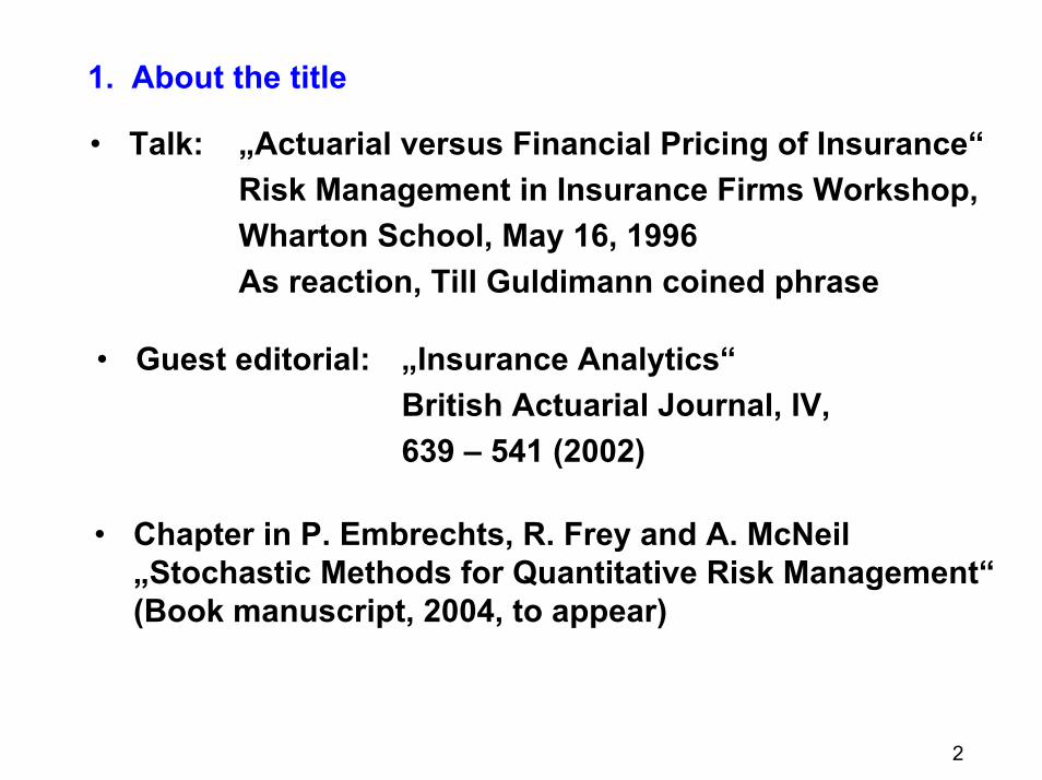
1. About the title
• Talk: „Actuarial versus Financial Pricing of Insurance“Risk Management in Insurance Firms Workshop,Wharton School, May 16, 1996As reaction, Till Guldimann coined phrase
• Guest editorial: „Insurance Analytics“British Actuarial Journal, IV,639 – 541 (2002)
• Chapter in P. Embrechts, R. Frey and A. McNeil„Stochastic Methods for Quantitative Risk Management“ (Book manuscript, 2004, to appear)
3
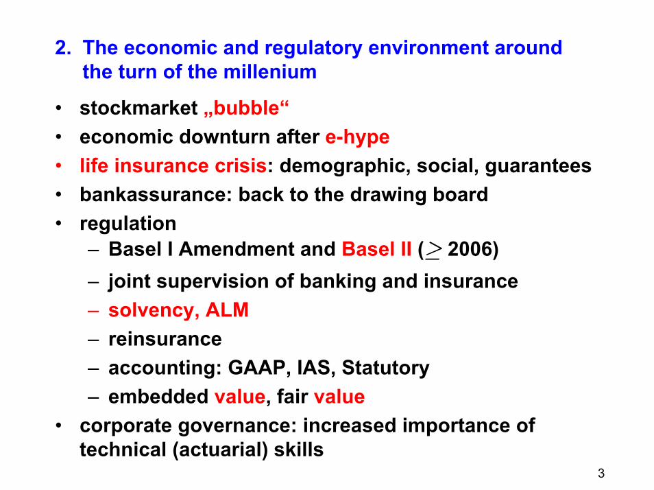
2. The economic and regulatory environment around the turn of the millenium
• stockmarket „bubble“• economic downturn after e-hype• life insurance crisis: demographic, social, guarantees• bankassurance: back to the drawing board• regulation
– Basel I Amendment and Basel II (≥ 2006)– joint supervision of banking and insurance– solvency, ALM– reinsurance– accounting: GAAP, IAS, Statutory– embedded value, fair value
• corporate governance: increased importance oftechnical (actuarial) skills
4
3. Question: where does that leave the actuary?
The Actuarial Profession:making financial sense of the future.
• Actuaries are respected professionals whose inno-vative approach to making business successful is motivated by a responsibility to the public interest.Actuaries identify solutions to financial problems.They manage assets and liabilities by analysing past events, assessing the present risks involved andmodelling what could happen in the future.
www.actuaries.org.uk
• Do we live up to this definition?
5
4. Insurance analytics: an incomplete list!
• incomplete markets• premium principles and risk measures• credibility theory• tail fitting
– analytic (models beyond normality)– algorithmic (Panjer, FFT)– asymptotic (Extreme Value Theory)
• scoring• dependence beyond correlation• stress testing techniques• dynamic solvency testing (ruin, DFA, ...)• long-term-horizon models
6
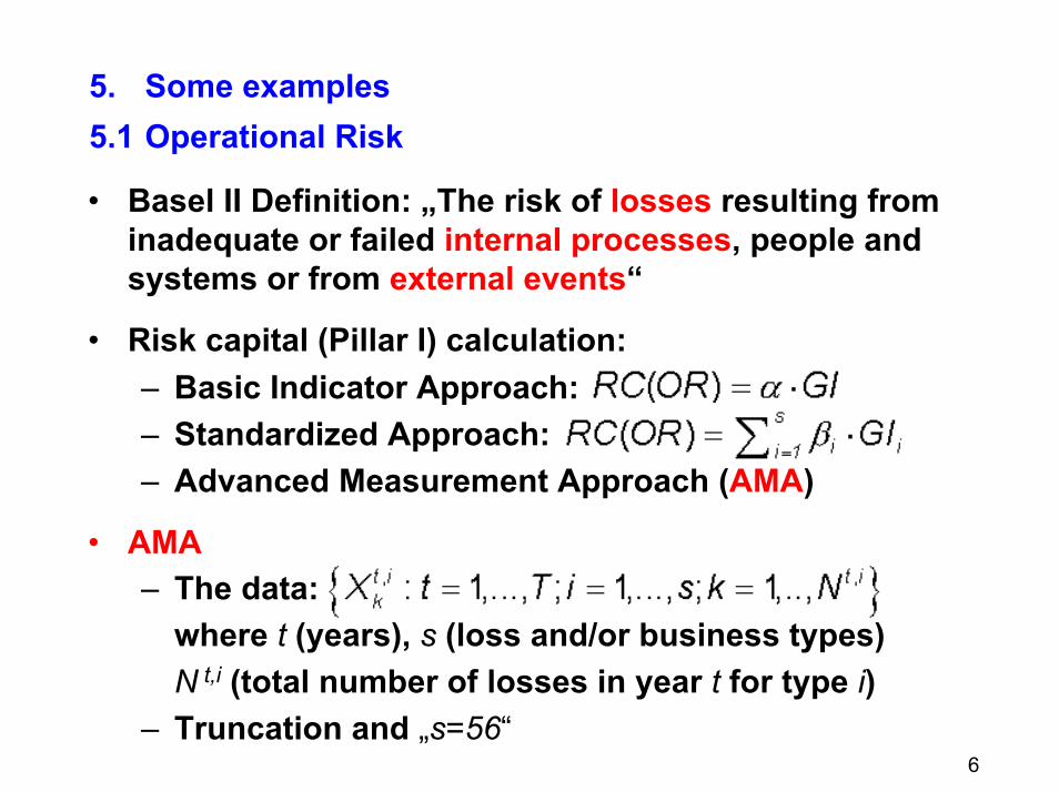
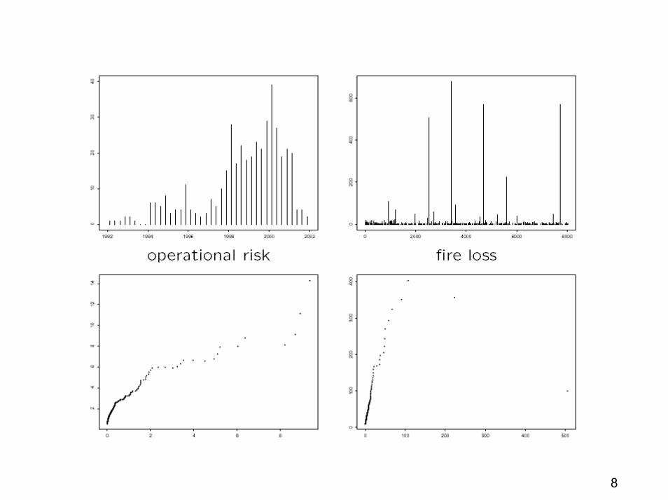
5. Some examples5.1 Operational Risk
• Basel II Definition: „The risk of losses resulting from inadequate or failed internal processes, people and systems or from external events“
• Risk capital (Pillar I) calculation:– Basic Indicator Approach:– Standardized Approach:– Advanced Measurement Approach (AMA)
• AMA– The data:
where t (years), s (loss and/or business types)N t,i (total number of losses in year t for type i)
– Truncation and „s=56“
7
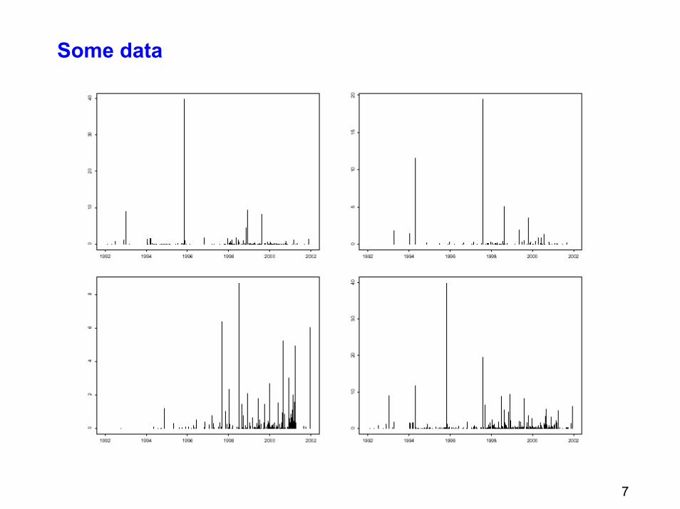
Some data
8
9
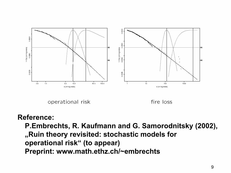
Reference: P.Embrechts, R. Kaufmann and G. Samorodnitsky (2002), „Ruin theory revisited: stochastic models foroperational risk“ (to appear)Preprint: www.math.ethz.ch/~embrechts
10
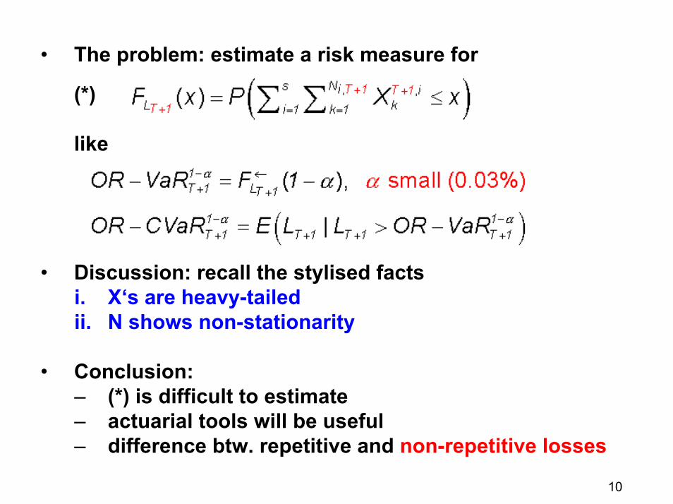
• The problem: estimate a risk measure for
(*)
like
• Discussion: recall the stylised factsi. X‘s are heavy-tailedii. N shows non-stationarity
• Conclusion:– (*) is difficult to estimate– actuarial tools will be useful– difference btw. repetitive and non-repetitive losses
11
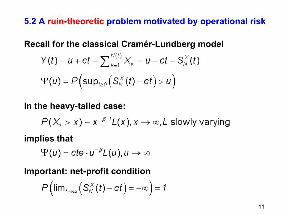
5.2 A ruin-theoretic problem motivated by operational risk
Recall for the classical Cramér-Lundberg model
In the heavy-tailed case:
implies that
Important: net-profit condition
12
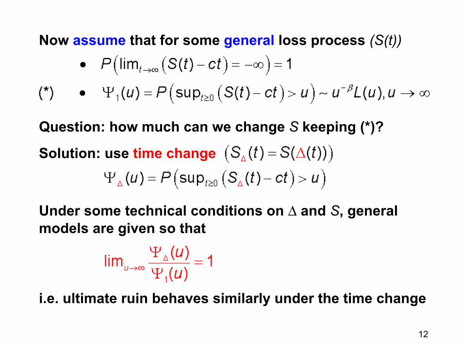
Now assume that for some general loss process (S(t))
Question: how much can we change S keeping (*)?
Solution: use time change
Under some technical conditions on D and S, generalmodels are given so that
i.e. ultimate ruin behaves similarly under the time change
13
Discussion
• time change:
• example:– start from the homogeneous Poisson case
(classical Cramér-Lundberg, heavy-tailed case)– use D to transform to changes in intensities
motivated by operational riskReference:
P. Embrechts and G. Samorodnitsky (2003) „Ruin problem and how fast stochastic processes mix“ Ann. Appl. Probab. (13), 1-36
– Lundberg-Cramér (1930‘s)– W. Doeblin (1940): Itô‘s lemma– Olsen q-time (1990‘s)– Geman et al. (1990‘s)– Monroe‘s theorem (1978)
14
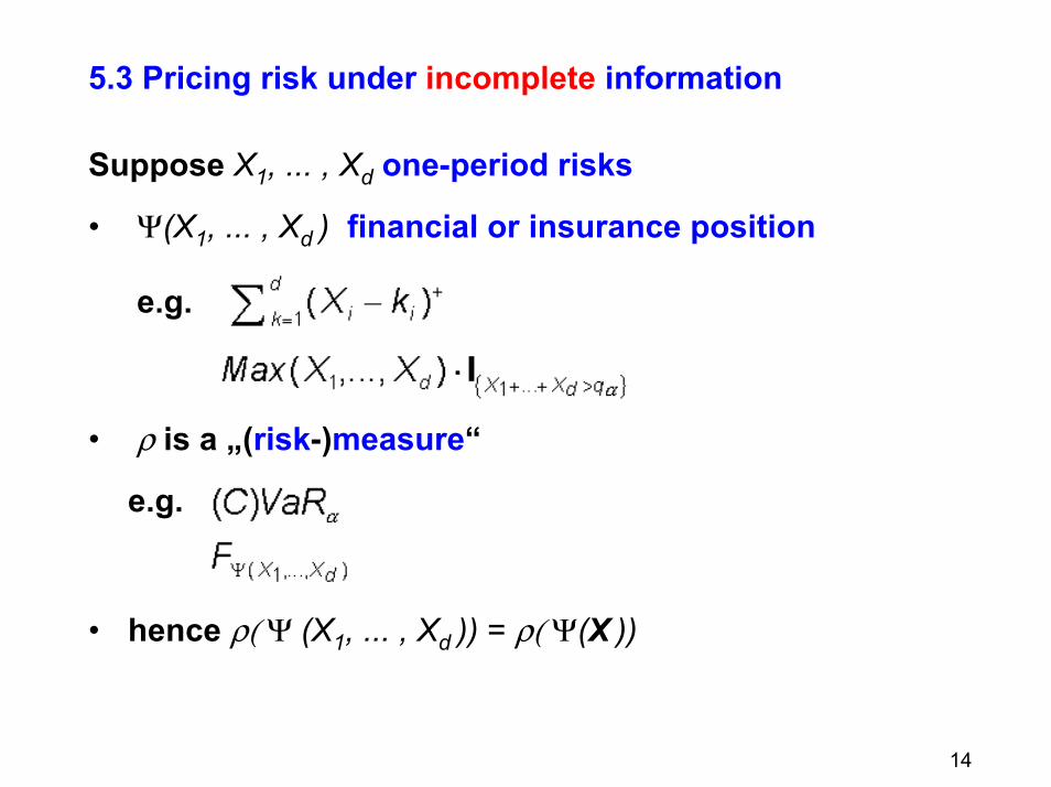
5.3 Pricing risk under incomplete information
Suppose X1, ... , Xd one-period risks
• Y(X1, ... , Xd ) financial or insurance position
e.g.
• r is a „(risk-)measure“
e.g.
• hence r( Y (X1, ... , Xd )) = r( Y(X ))
15
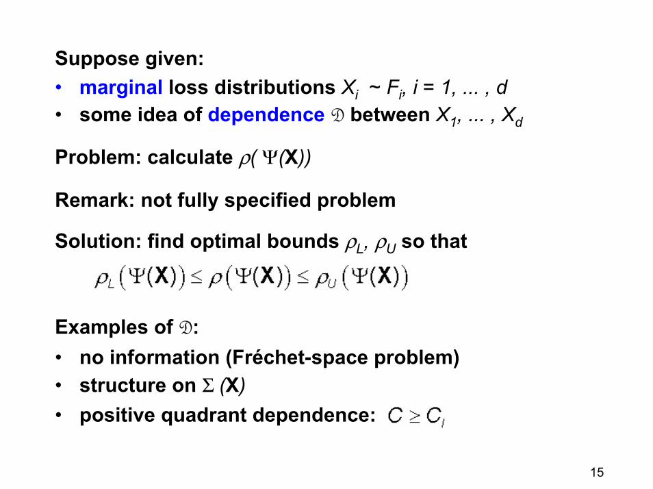
Suppose given:• marginal loss distributions Xi ~ Fi, i = 1, ... , d• some idea of dependence D between X1, ... , Xd
Problem: calculate r( Y(X))
Remark: not fully specified problem
Solution: find optimal bounds rL, rU so that
Examples of D:• no information (Fréchet-space problem)• structure on S (X)• positive quadrant dependence:
16
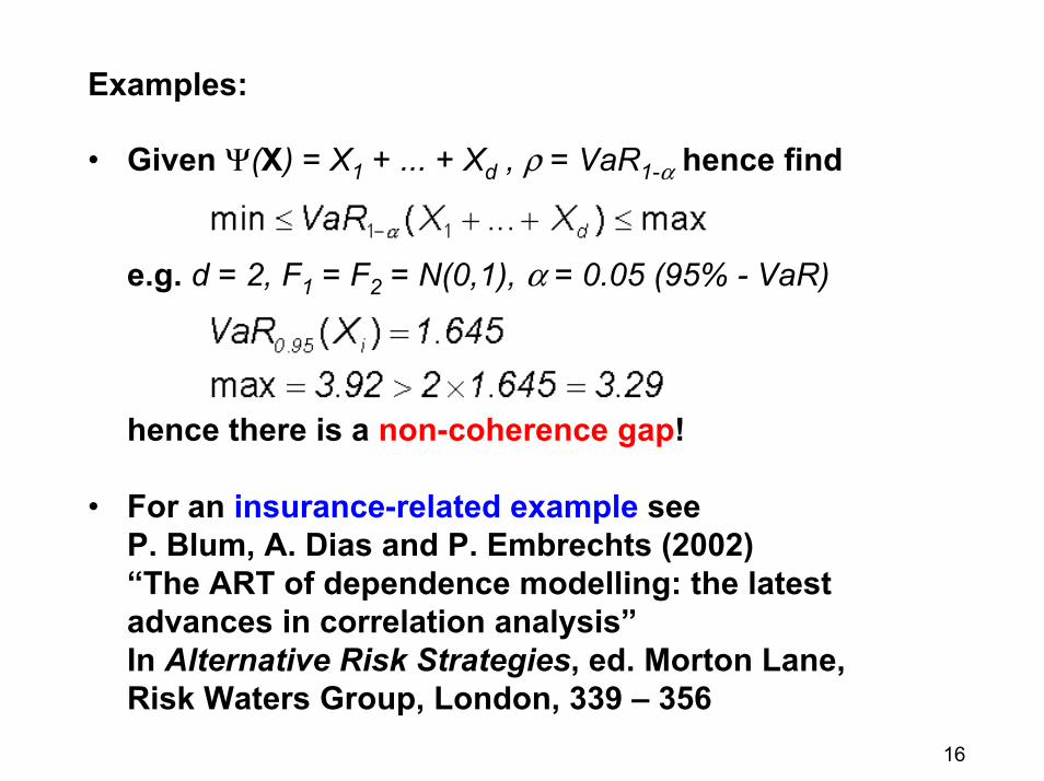
Examples:
• Given Y(X) = X1 + ... + Xd , r = VaR1-a hence find
e.g. d = 2, F1 = F2 = N(0,1), a = 0.05 (95% - VaR)
hence there is a non-coherence gap!
• For an insurance-related example seeP. Blum, A. Dias and P. Embrechts (2002)“The ART of dependence modelling: the latest advances in correlation analysis” In Alternative Risk Strategies, ed. Morton Lane, Risk Waters Group, London, 339 – 356
17
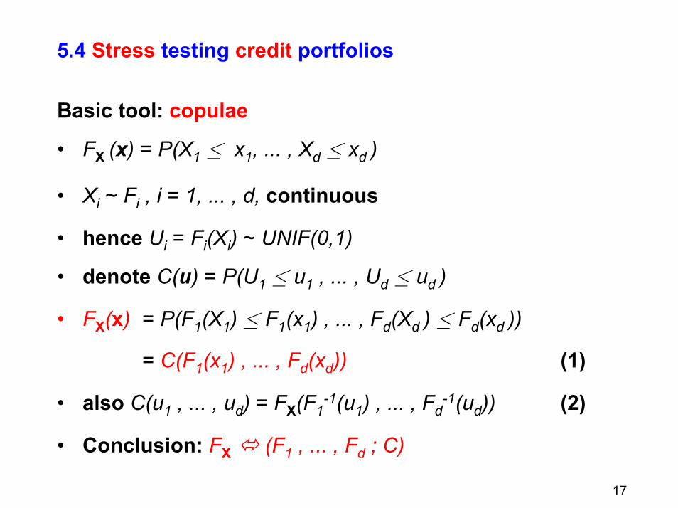
5.4 Stress testing credit portfolios
Basic tool: copulae
• FX (x) = P(X1 ≤ x1, ... , Xd ≤ xd )
• Xi ~ Fi , i = 1, ... , d, continuous
• hence Ui = Fi(Xi) ~ UNIF(0,1)
• denote C(u) = P(U1 ≤ u1 , ... , Ud ≤ ud )
• FX(x) = P(F1(X1) ≤ F1(x1) , ... , Fd(Xd ) ≤ Fd(xd ))
= C(F1(x1) , ... , Fd(xd)) (1)
• also C(u1 , ... , ud) = FX(F1-1(u1) , ... , Fd
-1(ud)) (2)
• Conclusion: FX (F1 , ... , Fd ; C)
18
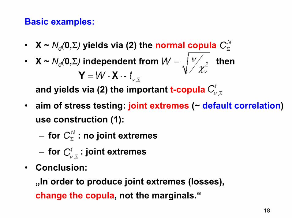
Basic examples:
• X ~ Nd(0,S) yields via (2) the normal copula
• X ~ Nd(0,S) independent from then
and yields via (2) the important t-copula
• aim of stress testing: joint extremes (~ default correlation)use construction (1):
– for : no joint extremes
– for : joint extremes
• Conclusion:„In order to produce joint extremes (losses),change the copula, not the marginals.“

19
Copula examples
20
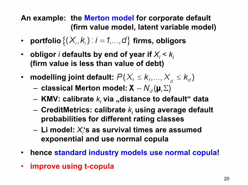
An example: the Merton model for corporate default(firm value model, latent variable model)
• portfolio firms, obligors
• obligor i defaults by end of year if Xi < ki(firm value is less than value of debt)
• modelling joint default:– classical Merton model: – KMV: calibrate ki via „distance to default“ data– CreditMetrics: calibrate ki using average default
probabilities for different rating classes– Li model: Xi‘s as survival times are assumed
exponential and use normal copula
• hence standard industry models use normal copula!
• improve using t-copula
21
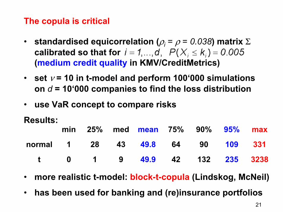
The copula is critical
• standardised equicorrelation (ri = r = 0.038) matrix Scalibrated so that for(medium credit quality in KMV/CreditMetrics)
• set n = 10 in t-model and perform 100‘000 simulationson d = 10‘000 companies to find the loss distribution
• use VaR concept to compare risks
Results:
32382351324249.9910t
331109906449.843281normal
max95%90%75%meanmed25%min
• more realistic t-model: block-t-copula (Lindskog, McNeil)
• has been used for banking and (re)insurance portfolios
22
Conclusion:
• actuaries have intersting tools to offer:insurance analytics
• stress testing (insurance and finance) portfolios is crucial
• think beyond normal distribution and normal dependence
• questions lead to important applications, and
• yield interesting academic research
• increased importance of integrated risk management
• many ... many more important issues exist: future ASTINs
References• check www.math.ethz.ch/finance