Intake epis food(): An R Function for Fitting a Bivariate

JSS Journal of Statistical SoftwareMarch 2012, Volume 46, Code Snippet 3. http://www.jstatsoft.org/

Intake_epis_food(): An R Function for Fitting a

Bivariate Nonlinear Measurement Error Model to

Estimate Usual and Energy Intake for Episodically

Consumed Foods

Adriana PerezThe University of Texas

Saijuan ZhangTexas A&M University

Victor KipnisNational Cancer Institute

Laurence S. FreedmanGertner Institute for Epidemiology

and Health Policy Research

Raymond J. CarrollTexas A&M University

Abstract

We consider a Bayesian analysis using WinBUGS to estimate the distribution of usualintake for episodically consumed foods and energy (calories). The model uses measuresof nutrition and energy intakes via a food frequency questionnaire along with repeated 24hour recalls and adjusting covariates. In order to estimate the usual intake of the food,we phrase usual intake in terms of person-specific random effects, along with day-to-dayvariability in food and energy consumption. Three levels are incorporated in the model.The first level incorporates information about whether an individual reported consumptionof a particular food item. The second level incorporates the amount of food consumptionequalling to zero if not consumed, and the third level incorporates the amount of energyintake. Estimates of posterior means of parameters and distributions of usual intakes areobtained by using Markov chain Monte Carlo calculations which can be thought as meanestimates for frequentists. This R function reports to users point estimates and credibleintervals for parameters in the model, samples from their posterior distribution, samplesfrom the distribution of usual intake and usual energy intake, trace plots of parametersand summary statistics of usual intake, usual energy intake and energy adjusted usualintake.

Keywords: excess zero models, MCMC, nonlinear mixed models, R, R2WinBUGS, zero-inflation.

http://www.jstatsoft.org/

2 Intake_epis_food(): A Bivariate Nonlinear Measurement Error Model in R

1. Introduction

There are many statistical challenges when modeling food intakes reported on two or more24 hours (24h) recalls. Some of the challenges involve the presence of measurement errorbecause estimating the distribution of usual intake of nutrients and foods in the populationinvolves monitoring and measuring such intakes over time and their associated recall biases.In addition, many consumers report episodically consumed foods, foods that are not typicallyconsumed every day. For example, fish may be reported in a particular day with a positiveintake, but on a different day fish intake may equal zero. Consequently, it is difficult toestimate nutrition intake with recall surveys when one of these recalls incorporate excess zeromeasurements. Data of this nature is often modeled with measurement error models withzero inflated data.

Recently, in nutritional surveillance (Tooze et al. 2006) and nutritional epidemiology (Kipniset al. 2009) two-part methods had been developed for analyzing episodically consumed foods.In the first part of the model, the probability of an episodically consumed food is estimatedusing logistic regression with a person-specific random effect. Then, in the second part ofthe model the amount of that episodically consumed food per day is modeled using linearregression on a transformed scale with also a person-specific effect. These two parts are linkedallowing that the two person-specific effects are correlated as well as by allowing commoncovariates in both parts of the model. This method is known as the “NCI method” (availableat http://riskfactor.cancer.gov/diet/usualintakes/) and described by Tooze et al.(2006) and Kipnis et al. (2009).

An extension into a three-part method that also incorporates the estimation of the amount ofenergy intake consumed per day is described in detail by Kipnis et al. (2011). These authorsestimated this three-part method using nonlinear mixed effects models with likelihoods com-puted by adaptive Gaussian quadrature in SAS software. However, computationally it wasfound to have serious convergence issues within the context of nutritional epidemiology andnutritional surveillance as indicated by Kipnis et al. (2011) and Zhang et al. (2011).

The goal of this article is to present a function for the implementation of this nonlinear mixedeffects model. The function Intake_epis_food() allows readers to input their data in R(R Development Core Team 2010) to generate and run the script of the three part model inWinBUGS (Spiegelhalter et al. 1999) and to run and obtain output simulations to R usingthe package R2WinBUGS (Sturtz et al. 2005). While the most important functions of thepackage R2WinBUGS are illustrated, we do not provide comprehensive documentation here;instead the reader is referred to the manual and online documentation with that package avail-able from the Comprehensive R Archive Network at http://CRAN.R-project.org/package=R2WinBUGS. In the next sections, the function and corresponding algorithms are explainedand an example is provided.

2. Method and parameter inference

The computational details of the Bayesian approach to fit the three-part model for an episod-ically consumed food and energy model (Kipnis et al. 2011) through Markov chain MonteCarlo (MCMC) techniques are provided by Zhang et al. (2011) with a brief summary givenhere. Our model takes into consideration measures of nutrition and energy intakes via a foodfrequency questionnaire (FFQ) along with two repeated 24h recalls and adjustment covari-

http://riskfactor.cancer.gov/diet/usualintakes/

http://CRAN.R-project.org/package=R2WinBUGS

http://CRAN.R-project.org/package=R2WinBUGS

Journal of Statistical Software – Code Snippets 3

ates. These two repeated 24h recalls provide information on the amounts of food and energyconsumed by each individual. Consequently, an indicator variable of whether the food wasconsumed can be generated from the reported amount of food consumed. In addition, be-cause two or more 24h recalls require distinguishing between and within person random error(Eckert et al. 1997), a type of classical measurement error is needed. Generally nutritionaldata are skewed, which may require transformations to reach normality and standardiza-tion. For person i = 1, . . . , n, and for the k = 1, 2 repeats of the 24h recall, the data areYik = (Yi1k, . . . , Yi3k)

>, where

Yi1k = Indicator of whether the food is consumed.

Yi2k = Amount of the food consumed as reported by the 24h recalls, which equals zeroif the food is not consumed.

Yi3k = Amount of energy consumed as reported by the 24h recalls.

We will use a Box-Cox transformation to account for the skewness in the data. The Box-Coxtransformation with transformation parameter λ, is h(y, λ) = (yλ−1)/λ if λ 6= 0, and h(y, λ)=log(y) if λ = 0. We will allow for the user to specify different transformation parameters λFand λE for food and energy intake, respectively.

After Box-Cox transformation, we further standardize and center these transformed variablesto have a mean of zero and variance of one. This is useful for making the prior distributionspecifications given below to be sensible and allows rapid convergence of the posterior samples.Specifically, let µλF and σλF be the mean and standard deviation of the transformed non-zero food data h(Yi2k, λF ), and let µλE and σλE be the mean and standard deviation of thetransformed energy data h(Yi3k, λE). Then, our analysis is performed using the followingtransformations:

Qi1k = Yi1k; (1)

Qi2k =√

2 Yi1k h(Yi2k, λF )− µλF /σλF ; (2)

Qi3k =√

2 h(Yi3k, λE)− µλE /σλE = htr(Yi3k, λE , µλE , σλE ); (3)

There are also covariates such as age category, ethnic status and, in many cases the results ofreported intakes from a food frequency questionnaire. In principle, the covariates can differbased on the three types of data, so we denote them as Vi1, Vi2, Vi3, which are vector-valued.To improve linearity and homoscedasticity of the model, we follow the recommendations of(i) implementing Box-Cox transformations on all or some covariates like intakes from a foodfrequency questionnaire (Kipnis et al. 2009), (ii) centering and (iii) scaling on all covariates.Without loss of generality, let λc represent a vector containing the Box-Cox transformationparameter used for covariates. Let µλc and σλc be the vector means and standard deviationsof the transformed covariates. Then, these transformed, center and scaled covariates aredenoted by:

Xi1 = h(Vi1, λc)− µλc/σλc (4)



Let (Ui1, Ui2, Ui3) = Normal(0,Σu) be random effects associated with consumption, amount(if the food is consumed), and energy. Similarly, for k = 1, 2, (εi1k, εi2k, εi3k) = Normal(0,Σε)


accounts for day-to-day variation. The model for whether there is consumption can be statedas:

P(Qi1k = 1|Xi1, Ui1, Ui2, Ui3) = Φ(α1 +X>i1β1 + Ui1), (7)

where Φ(·) is the standard normal distribution function and (Wi1k,Wi2k,Wi3k) represent theircorresponding latent variables as follows. A food being consumed at visit k is equivalent to

Qi1k = 1 ⇐⇒ Wi1k = α1 +X>i1β1 + Ui1 + εi1k > 0. (8)

The food when consumed and energy intake are modeled as

[Qi2k|Qi1k > 0] = Wi2k = α2 +X>i2β2 + Ui2 + εi2k (9)

[Qi3k] = Wi3k = α3 +X>i3β3 + Ui3 + εi3k. (10)

The prior distribution of parameters β1, β2, β3 is assumed to be multivariate Normal withvector mean 0 and variance covariance Σu. An inverse Wishart denoted as IW(Ωu,mu) priorwas specified for Σu. We set Ωu to have an exchangeable correlation structure with startingvalues with diagonal entries all equal to 1 and correlations 0.5. We have two necessaryrestrictions on Σε: (i) εi1k and εi2k are independent; and (ii) var(εi1k) = 1, so that β1 isidentifiable, along with the distribution of Ui1. Furthermore, we constrained this covariancematrix using a polar coordinate representation with γ ∈ (−1, 1) and θ ∈ (−π, π). With theseconsiderations Σε can be written as:

Σε =

1 0 p1s1/233

0 s22 p2(s22s33)1/2

p1s1/233 p2(s22s33)

1/2 s33

, (11)

where p1 = γcos(θ) and p2 = γsin (θ). The recommended prior distributions for s22 and s33are Uniform(0, 3), for γ is Uniform(−1, 1) and for θ is Uniform(−π, π) (Zhang et al. 2011).The corresponding inverse of Σu is a Wishart distribution denoted as Σ−1u =W(Ω−1u ,mu), andthe inverse of Σε can be written as:

Σ−1ε =

1 + wp12s33 wp1p2s33s

−1/222 −wp1s1/233

wp1p2s33s−1/222 s−122 + wp22s33s

−122 −wp2s1/233 s

−1/222

−wp1s1/233 −wp2s1/233 s−1/222 w

, (12)

where w = s33(1− p21 − p22)−1.

Usual intake analysis

Besides the parameters and the random effects (Ui1, Ui2, Ui3) in this context it is vital to alsohave the posterior samples of usual intake TFi, usual energy intake TEi, and energy adjustedusual intake 1000TFi/TEi, all on the original scale. We used the best-power method (Doddet al. 2006) for estimating both usual energy intake and usual intake for person i. We firstconsider energy:

TEi = Eh−1tr (α3 +X>i3β3 + Ui3 + εi3, λE , µλE , σλE )|Xi3, Ui3

(13)

≈ h∗tr

α3 +X>i3β3 + Ui3, λE , µλE , σλE ,Σε(3, 3)

. (14)


where

h∗trv, λ, µ, σ,Σ = h−1tr (v, λ, µ, σ) +Σ

2

∂2h−1tr (v, λ, µ, σ)

∂v2.

Similarly, a person’s usual intake of the dietary component on the original scale is defined as

TFi = Φ(α1 +X>i1β1 + Ui1)h∗tr

α2 +X>i2β2 + Ui2, λF , µλF , σλF ,Σε(2, 2)

. (15)

When λ = 0, the back-transformation and second derivative are:

h−1tr (v, 0, µ, σ) = exp(µ+ σv/√

2);

∂2h−1tr (v, 0, µ, σ)/∂v2 = σ2h−1tr (v, 0, µ, σ)/2.

Similarly, when λ 6= 0, the back-transformation and second derivative are:

h−1tr (v, λ, µ, σ) = (1 + λµ+ λσv/√

2)1/λ;

∂2h−1tr (v, λ, µ, σ)/∂v2 =σ2

2(1− λ)(1 + λµ+ λσv/

√2)−2+1/λ.

3. Using the Intake_epis_food() function in R

Users must install the R2WinBUGS (Sturtz et al. 2005) package in R and WinBUGS (Spiegel-halter et al. 1999) before running Intake_epis_food() function. This function assumes thatthere are no missing observations. Intake_epis_food() loads the packages R2WinBUGS,stats, and timeSeries (Wurtz and Chalabi 2011) automatically.

The Intake_epis_food() function incorporates this three-part model, with truncated nor-mal random variables for generating the latent Wi1k, and Metropolis-Hastings computationsfor α1, α2, α3, β1, β2, β3, the elements of Σu, and Σε. This function generates and runs thescript of this model in WinBUGS and returns a MCMC computation. We emphasize thatthe MCMC computation can either be thought of as a strictly Bayesian computation withordinary Bayesian inference, or as a means of developing frequentist estimators of the crucialparameters. This MCMC computation produces estimates which are known to be asymp-totically equivalent to maximum likelihood estimators, which are difficult to obtain (Zhanget al. 2011). In Bayesian terms we used the posterior means of the model. Users are notonly interested in estimates of usual energy intake (Equation 14) and usual intake for personi (Equation 15) but also in the energy-adjusted usual intake 1000TFi/TEi.

The Intake_epis_food() function produces seven output files. The first output file containsparameter estimates (posterior means) of: α1 and β1 from Equation 8; α2 and β2 fromEquation 9; and α3 and β3 from Equation 10. Also, the first output file contains parameterestimates for Σµ, Σ−1µ , Σε, and Σ−1ε . The second output file contains summary statisticsof Bayesian estimates of Equation 14, Equation 15, and the energy-adjusted usual intake1000TFi/TEi. The third output file contains the iterations from the MCMC computations.The fourth output file contains summary statistics of Bayesian estimates for Ui1, Ui2, Ui3. Thefifth output file contains trace plots of the intercept and coefficients in Equation 8, Equation 9,and Equation 10. The sixth output file contains trace plots of the variance-covariances Σµ,Σ−1µ , Σε and Σ−1ε . The seventh output file contains density plots of Equation 15 and theenergy adjusted usual intake 1000TFi/TEi.

The defaults for the Intake_epis_food() function in R are:


Intake_epis_food(data.file.name = "data.file.name",

numcov = 4, df = 5, lambdaf = 0.32, lambdae = 0.23, lvar1 = 999,

lvar2 = 999, lvar3 = 0.33, lvar4 = 0, n.iter = 11000, n.chains = 1,

n.burnin = 1000, n.thin = 10, bugs.seed = 123456,

working.directory = "working.directory", file.estimates = "estimates.csv",

file.istats = "estimates_intake.csv", file.iterations = "iterations.csv",

file.uis = "uis.csv", file.tracep = "trace_plots.pdf",

file.tpvarcov = "trace_plot_var_cov_matrices.pdf",

file.densityp = "density_plots.pdf",

bugs.directory = "c:/Program Files/WinBUGS14/")

with the following arguments:

Data.file.name: Name of the file containing the data (default: "data.file.name") in thefollowing order:

The first variable identifies individuals, e.g., an ID number.

The next two variables are the 24h recalls variables of food intake, in order.

The next two variables are the 24h recalls variables of energy intake, in order.

The next variables are the covariates, and cannot have a column of ones. We haveset the number of covariates to four, given that each covariate may have a differentBox-Cox transformation parameter.

numcov: Number of covariates in user’s dataset (default: 4).

df: Number of the degrees of freedom of mu (default: 5).

lambdaf: Value of λF to be used for transformation of food intake (default: 1 indicating notransformation done).

lambdae: Value of λE to be used for transformation of energy intake (default: 1 indicatingno transformation done).

lvar1: Value of λc to be used for Box-Cox transformation of first covariable (default: 999

indicating no transformation done).

lvar2: Value of λc to be used for Box-Cox transformation of second covariable (default: 999indicating no transformation done).

lvar3: Value of λc to be used for Box-Cox transformation of third covariable (default: 999

indicating no transformation done).

lvar4: Value of λc to be used for Box-Cox transformation of fourth covariable (default: 999indicating no transformation done).

n.iter: Number of iterations of the MCMC. Please include the number of burning iterationsalso (default: 11000).

n.chains: Number of chains (default: 1).

n.burnin: Number of burn-in iterations of the MCMC (default: 1000).


n.thin: Thinning rate of the MCMC (default: 10).

bugs.seed: Random seed to be used for the MCMC (default: 123456).

working.directory: Drive and folder location for output files from WinBUGS (default:"C:").

file.estimates: Name of the file to save posterior summary statistics including mean, stan-dard deviation as well as percentiles: 2.5th, 25th, 50th, 75th and 97.5th (default:"estimates.csv"), of α1, α2, α3, β1, β2, β3 from Equation 8, Equation 9, and Equa-tion 10 as well as Σµ, Σ−1µ , Σε, and Σ−1ε .

file.istats: Name of the file to save summary statistics of usual food intake, Equation 15,usual energy intake, Equation 14, and usual food intake per 1000 calories (1000TFi/TEi)(default: "estimates_intake.csv").

file.iterations: Name of the file to save iterations (default: "iterations.csv"). Thenumber of iterations saved corresponds to (n.iter - n.burnin)/n.thin.

file.uis: Name of the file to save summary statistics of Bayesian estimates (default:"uis.csv") for Ui1, Ui2, Ui3 including mean, standard deviation as well as percentiles:2.5th, 25th, 50th, 75th and 97.5th for person i = 1, . . . , n. The first variable given in thedataset that identifies individuals is included as the first variable in this file for linkingpurposes to users.

file.tracep: Name of the file to save trace plots of parameters (default:"trace_plots.pdf").

file.tpvarcov: Name of the file to save trace plots of variance-covariances Σµ, Σ−1µ , Σε andΣ−1ε (default: "trace_plot_var_cov_matrices.pdf").

file.densityp: Name of the file to save density plots of usual food intake and usual foodintake per 1000 calories. Each one is generated individually and an overlayed plot isgenerated as well (default: "density_plots.pdf").

bugs.directory: Drive and folder location of WinBUGS (default: "c:/Program Files/

WinBUGS14/").

Once the data is input, Intake_epis_food() invokes WinBUGS from R. WinBUGS requiresa file describing the model in Equation 8, Equation 9, Equation 10 in Section 2. This model isincluded as file intake_program.txt and is loaded in R using its bugs() argument. Althoughthe default priors of the constrained variance-covariance matrix of random errors are gearedto the pre-standardization of the data as described in Section 2, the user may change thoseprior entries within the file intake_program.txt, possibly changing any code described inTable 1.

Also, users may change any of the default values of Intake_epis_food() function whenthe function is called to run by replacing those arguments in the last sentence of the fileaccompanied by this paper. The MCMC posterior means of α1, α2, α3, β1, β2, β3, the elementsof Σu, Σε, Σ−1u and Σ−1ε are displayed on the screen of R by Intake_epis_food() andsaved automatically in numeral matrices on file names previously listed. See Section 4 for anexample.


Matrix notation Default distribution and range Code in intake_program.txt

s22 Uniform(0, 3) tau.e1 ~ dunif(0, 3)

s33 Uniform(0, 3) tau.e2 ~ dunif(0, 3)

γ Uniform (−1, 1) a.e1 ~ dunif(-0.99, 0.99)

θ Uniform (−1, 1) a.e2 ~ dunif(-3.11, 3.11)

Table 1: Constrained variance-covariance matrix of random errors.

4. Application of the Intake_epis_food() function

We simulated data using parameter values identified from the calibration sub-study of theNational Institutes of Health (NIH) and the American Association of Retired Persons (AARP)Diet and Health Study (Schatzkin et al. 2001). The NIH-AARP study is a cohort composedof people who resided in one of six states: California, Florida, Pennsylvania, New Jersey,North Carolina, and Louisiana or in two metropolitan areas: Atlanta, Georgia and Detroit,Michigan. From 1995 through 1996, 3.5 million questionnaires were mailed to members ofthe AARP, aged 50–71 years. The questionnaire included a dietary section as well as somelifestyle questions. Over 500,000 people returned the questionnaire after three mailing waves.This, then, is the largest study of diet and health ever conducted in the USA. In 1996–1997, these participants received a risk-factor questionnaire which asked additional questionsabout lifestyle and behavior, and in 2004–2006 these participants received another follow-upquestionnaire (available at http://dietandhealth.cancer.gov/resource/).

Participants for the calibration study were randomly selected from the 46,970 subjects whohad responded to the first wave as of January 1996. Two thousand participants was thetargeted sample size to attempt recruitment calls for a baseline and 24h follow up. The sampleavailable to us included 920 men. Because the data are not publicly available, we simulated920 food intakes that are similar in distribution to the men in the NIH-AARP calibrationstudy. We used as X>ik four covariates: Age, body mass index (BMI), consumption of servingsof whole grains from the FFQ, and energy intake from the FFQ. Therefore, Σ−1u requires toestimate 3x3 = 9 parameters, after subtracting four covariates estimated, then the degreesof freedom of the inverse Wishart were setup as mu = 5. The latter two covariates weretransformed by the cube root and the logarithm, respectively.

We present results from Intake_epis_food() for this simulated data example with a sam-ple size of 920 men, modeling whole grains consumption. We used a burn-in of 1, 000 stepsfollowed by 10, 000 MCMC iterations. These values were the same arbitrary values used em-pirically in our MATLAB code (Zhang et al. 2011). Our Intake_epis_food() function tookapproximately 6 hours and 16 minutes (Pentium computer D CPU 3.5GHz and 1.99GB ofRAM). We used only every 10th value of the chain. The first output file contains the av-erage over 10,000 MCMC of posterior mean, posterior standard deviation, posteriors: 2.5thpercentile, 25th percentile, 50th percentile, 75th percentile and 97.5th percentile. The inter-cepts of the model are α1, α2, α3 corresponding to each level of the three-part model. Also,estimates of regression parameters for each covariate appear for each level of the model. Thisis the notation used for the output:

alpha_1: Represents the intercept in Equation 8.


http://dietandhealth.cancer.gov/resource/



beta_1_j: Represents the estimated coefficient of the jth covariate in Equation 8,j = 1, . . . , numcov.



tau_j_p: Represents the (j, p) entry estimate of Σ−1u , j = p = 1, 2, 3.

sigma2_j_p: Represents the (j, p) entry estimate of Σu, j = p = 1, 2, 3.

a.e1: Represents the estimate of γ.

a.e2: Represents the estimate of θ.

sigmaemat_j_p: Represents the (j, p) entry estimate of Σε, j = p = 1, 2, 3, with Σε11=1 andΣε12=Σε21=0.

tauemat_j_p: Represents the the (j, p) entry estimate of Σ−1ε , j = p = 1, 2, 3.

We used λF = 0.32 as the Box-Cox transformation parameter of food intake λE = 0.23 asthe Box-Cox transformation of energy intake. We setup our working directory in R with thecommand setwd("C:") and using Intake_epis_food() function:

R> Intake_epis_food(data.file.name = "Sim_AARP_wg_Men.csv",

+ numcov = 4, df = 5, lambdaf = 0.32, lambdae = 0.23, lvar1 = 999,

+ lvar2 = 999, lvar3 = 0.33, lvar4 = 0, n.iter = 11000, n.chains = 1,

+ n.burnin = 1000, n.thin = 10, bugs.seed = 123456,

+ working.directory = "C:/", file.estimates = "estimates.csv",

+ file.istats = "estimates_intake.csv",

+ file.iterations = "iterations.csv", file.uis = "uis.csv",

+ file.tracep = "trace_plots.pdf",

+ file.tpvarcov = "trace_plot_var_cov_matrices.pdf",

+ file.densityp = "density_plots.pdf",

+ bugs.directory = "c:/Program Files/WinBUGS14/")

After calculations, estimates of α1, α2, α3, β1, β2, β3, Σµ, Σ−1µ , Σε, and Σ−1ε , are shown as wellas summary statistics using a Bayesian approach for three variables are provided immediatelyin the console screen (a) food usual intake, (b) usual food intake per 1000 calories, and(c) energy usual intake. The following shows the results for whole grains.

Inference for Bugs model at ' Intake_program.txt ', fit using WinBUGS,

1 chains, each with 11000 iterations (first 1000 discarded)

n.thin= 10 n.sims= 1000 iterations saved

mean sd 2.5% 25% 50% 75% 97.5%

alpha_1 0.89 0.06 0.79 0.85 0.89 0.92 1.00


alpha_2 -0.04 0.05 -0.13 -0.07 -0.04 -0.01 0.05

alpha_3 0.00 0.04 -0.07 -0.03 0.00 0.02 0.07

beta_1_1 0.16 0.05 0.07 0.13 0.16 0.19 0.25

beta_1_2 -0.08 0.05 -0.18 -0.12 -0.08 -0.05 0.00

beta_1_3 0.57 0.05 0.47 0.54 0.57 0.61 0.67

beta_1_4 -0.29 0.05 -0.38 -0.32 -0.29 -0.26 -0.19

beta_2_1 -0.07 0.04 -0.15 -0.09 -0.06 -0.04 0.01

beta_2_2 -0.08 0.04 -0.16 -0.11 -0.08 -0.06 -0.01

beta_2_3 0.42 0.04 0.34 0.40 0.42 0.45 0.50

beta_2_4 -0.11 0.04 -0.18 -0.13 -0.11 -0.08 -0.03

beta_3_1 -0.07 0.04 -0.15 -0.10 -0.07 -0.05 0.00

beta_3_2 -0.06 0.04 -0.14 -0.09 -0.06 -0.04 0.00

beta_3_3 0.00 0.04 -0.07 -0.03 0.00 0.03 0.08

beta_3_4 0.34 0.04 0.27 0.32 0.34 0.37 0.42

tau_1_1 2.05 0.57 1.26 1.66 1.94 2.31 3.50

tau_1_2 -0.33 0.60 -1.64 -0.66 -0.31 0.04 0.82

tau_1_3 -0.11 0.19 -0.47 -0.23 -0.11 0.01 0.29

tau_2_1 -0.33 0.60 -1.64 -0.66 -0.31 0.04 0.82

tau_2_2 3.29 0.79 2.21 2.77 3.13 3.62 5.31

tau_2_3 -0.57 0.28 -1.21 -0.73 -0.54 -0.38 -0.09

tau_3_1 -0.11 0.19 -0.47 -0.23 -0.11 0.01 0.29

tau_3_2 -0.57 0.28 -1.21 -0.73 -0.54 -0.38 -0.09

tau_3_3 1.53 0.16 1.26 1.42 1.51 1.63 1.89

sigma2_1_1 0.56 0.13 0.33 0.47 0.55 0.64 0.83

sigma2_1_2 0.06 0.09 -0.12 0.00 0.06 0.12 0.22

sigma2_1_3 0.06 0.06 -0.06 0.02 0.06 0.10 0.18

sigma2_2_1 0.06 0.09 -0.12 0.00 0.06 0.12 0.22

sigma2_2_2 0.37 0.07 0.23 0.32 0.36 0.41 0.51

sigma2_2_3 0.13 0.05 0.03 0.10 0.13 0.16 0.23

sigma2_3_1 0.06 0.06 -0.06 0.02 0.06 0.10 0.18

sigma2_3_2 0.13 0.05 0.03 0.10 0.13 0.16 0.23

sigma2_3_3 0.72 0.07 0.60 0.68 0.72 0.77 0.86

a.e1 0.17 0.05 0.09 0.14 0.17 0.20 0.26

a.e2 0.81 0.29 0.28 0.62 0.80 0.99 1.37

sigmaemat_1_3 0.12 0.05 0.03 0.09 0.12 0.16 0.23

sigmaemat_2_2 1.26 0.08 1.11 1.21 1.26 1.31 1.42

sigmaemat_2_3 0.14 0.05 0.04 0.11 0.14 0.18 0.24

sigmaemat_3_1 0.12 0.05 0.03 0.09 0.12 0.16 0.23

sigmaemat_3_2 0.14 0.05 0.04 0.11 0.14 0.18 0.24

sigmaemat_3_3 1.16 0.06 1.06 1.12 1.16 1.19 1.27

tauemat_1_1 1.02 0.01 1.00 1.01 1.01 1.02 1.05

tauemat_1_2 0.01 0.01 0.00 0.01 0.01 0.02 0.03

tauemat_1_3 -0.11 0.05 -0.21 -0.14 -0.11 -0.08 -0.03

tauemat_2_1 0.01 0.01 0.00 0.01 0.01 0.02 0.03

tauemat_2_2 0.81 0.05 0.72 0.78 0.81 0.84 0.91

tauemat_2_3 -0.10 0.04 -0.17 -0.13 -0.10 -0.08 -0.03

tauemat_3_1 -0.11 0.05 -0.21 -0.14 -0.11 -0.08 -0.03


0.0 0.5 1.0 1.5 2.0

0.0

0.5

1.0

1.5

Den

sity

Figure 1: The solid line is the posterior density estimate of the mean for whole grains usualintake from 1000 MCMC. The dashed line is the posterior density estimate of the mean forwhole grains usual intake per 1000 calories.

tauemat_3_2 -0.10 0.04 -0.17 -0.13 -0.10 -0.08 -0.03

tauemat_3_3 0.89 0.04 0.81 0.87 0.89 0.92 0.98

Usual food intake Usual food intake per 1000 calories Energy usual intake

Mean 0.9359701 0.4072328 2298.3852

S.d. 0.6947905 0.2849965 446.3253

5th 0.1887330 0.0823138 1636.7102

10th 0.2632069 0.1156591 1755.9317

25th 0.4359173 0.1992969 1982.9681

50th 0.7421419 0.3408097 2267.2364

75th 1.2117088 0.5350990 2568.3280

90th 1.9042402 0.7920862 2891.3676

95th 2.3828280 0.9484864 3088.9744

This is the only output presented in the console screen. However, these results are saved infile.estimates and file.istats respectively. Five additional output files are stored asmentioned before, but examples of these files are not presented here. Instead, we present theposterior density of the mean of usual whole grains intake plot and the posterior density of themean of usual whole grains intake per 1000 calories in Figure 1 (file.densityp). We presenttrace plots of the intercept and coefficients in Equation 8, Equation 9, and Equation 10 inFigure 2 (file.tracep). We present trace plots of entry estimates saved in file.tpvarcov

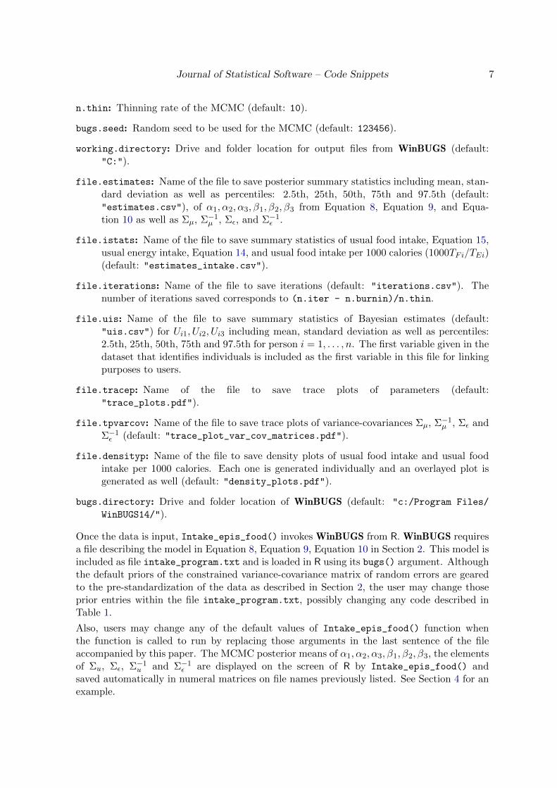
of variance-covariance matrices (i) for Σµ in Figure 3 (first three rows), (ii) for Σ−1µ in Figure 3(last three rows), (iii) for Σε in Figure 4 and (iv) for Σ−1ε in Figure 5.


Figure 2: First column shows trace plots of parameters for the intercept, age, body mass index,consumption of whole grains and energy intake from whole grains in Equation 8. Secondcolumn shows trace plots of parameters for the intercept, age, body mass index, consumptionof whole grains and energy intake from whole grains in Equation 9. Third column shows traceplots of parameters for the intercept, age, body mass index, consumption of whole grains andenergy intake from whole grains in Equation 10. Trace plot were computed from 1000 MCMCof intercepts and estimated coefficients.


Figure 3: Trace plot of variance-covariance matrix estimates of Σµ (first three rows) and Σ−1µ(last three rows), j = p = 1, 2, 3, generated from 1000 MCMC for each entry.


Figure 4: Trace plot of variance-covariance matrix estimates Σε j=p=1,2,3, generated from1000 MCMC for each entry. The following parameters are neither estimated nor plottedbecause they are fixed: Σε11=1 and Σε12=Σε21=0.

5. Discussion

This paper was motivated by the AARP calibration sub-study in nutritional epidemiology.Our main aim when implementing this function was to help users to estimate this recentnonlinear mixed three-part model of measurement error for an episodically food consumed ina Bayesian manner. Readers can evaluate if any of the parameters are different from zero byusing the credible intervals reported. Similarly, not only posterior means are provided as wellas medians and difference percentiles to facilitate interpretations of results for the users. Thisfunction has some limitations. This R function is implemented in its applicability to data withonly two 24h recalls and four covariates. If users have more than 24h recalls and/or a differentnumber of variates than four, users will need to modify not only the R code but also the Win-BUGS model provided, accordingly. Although, our example was setup to run only one chain,due to the amount of time the program requires to run, users can use multiple chains. Wecaution users who work under Windows 7 operating system to make sure to read the instruc-tions on how to make WinBUGS to run under it (available at http://windows.microsoft.com/en-US/windows-vista/Make-older-programs-run-in-this-version-of-Windows).

Acknowledgments

This research was supported by a grant from the National Cancer Institute (R37-CA-057030).

http://windows.microsoft.com/en-US/windows-vista/Make-older-programs-run-in-this-version-of-Windows

http://windows.microsoft.com/en-US/windows-vista/Make-older-programs-run-in-this-version-of-Windows


Figure 5: Trace plot of variance-covariance matrix estimates Σ−1ε j = p = 1, 2, 3, generatedfrom 1000 MCMC each entry.

Dr. Perez was also supported by a grant from the Michael and Susan Dell Foundation duringthe writing of this paper. We thank Laura Bellamy and Raja I. Malkani for proofreading thismanuscript.

References

Dodd KW, Guenther PM, Freedman LS, Subar AF, Kipnis V, Midthune D, Tooze JA, Krebs-Smith SM (2006). “Statistical Methods for Estimating Usual Intake of Nutrients and Foods:A Review of the Theory.” Journal of the American Dietetic Association, 106(10), 1640–1650.

Eckert RS, Carroll RJ, Wang N (1997). “Transformations to Additivity in Measurement ErrorModels.” Biometrics, 53, 262–272.

Kipnis V, Freedman LS, Carroll RJ, Midthune D (2011). “A Measurement Error Model forEpisodically Consumed Foods and Energy.” Preprint.

Kipnis V, Midthune D, Buckman DW, Dodd KW, Guenther PM, Krebs-Smith SM, SubarAF, Tooze JA, Carroll RJ, Freedman, S L (2009). “Modeling Data with Excess Zerosand Measurement Error: Application to Evaluating Relationships between EpisodicallyConsumed Foods and Health Outcomes.” Biometrics, 65(4), 1003–1010.


R Development Core Team (2010). R: A Language and Environment for Statistical Computing.R Foundation for Statistical Computing, Vienna, Austria. ISBN 3-900051-07-0, URL http:

//www.R-project.org/.

Schatzkin A, Subar AF, Thompson FE, Harlan LC, Tangrea J, Hollenbeck AR, HurwitzPE, Coyle L, Schussler N, Michaud DS, Freedman LS, Brown CC, Midthune D, Kipnis V(2001). “Design and Serendipity in Establishing a Large Cohort with Wide Dietary IntakeDistributions: The National Institutes of Health-AARP Diet and Health Study.” AmericanJournal of Epidemiology, 154, 1159–1125.

Spiegelhalter DJ, Thomas A, Best NG (1999). WinBUGS Version 1.2 User Manual. MRCBiostatistics Unit, Cambridge, UK. URL http://www.mrc-bsu.cam.ac.uk/bugs/.

Sturtz S, Ligges U, Gelman A (2005). “R2WinBUGS: A Package for Running WinBUGSfrom R.” Journal of Statistical Software, 12(3), 1–16. URL http://www.jstatsoft.org/

v12/i03/.

Tooze JA, Midthune D, Dodd KW, Freedman LS, Krebs-Smith SM, Subar AF, Guenther PM,Carroll RJ, Kipnis V (2006). “A New Statistical Method for Estimating the Usual Intakeof Episodically Consumed Foods with Application to Their Distribution.” Journal of theAmerican Dietetic Association, 106(10), 1575–1587.

Wurtz D, Chalabi Y (2011). timeSeries: Rmetrics – Financial Time Series Objects.R package version 2130.92, URL http://CRAN.R-project.org/package=timeSeries.

Zhang S, Krebs-Smith S, Midthune D, Perez A, Buckman DW, Kipnis V, Freedman LS, DoddKW, Carroll RJ (2011). “Fitting a Bivariate Measurement Error Model for EpisodicallyConsumed Dietary Components.”The International Journal of Biostatistics, 7(1), Article 1.

Affiliation:

Adriana PerezDivision of Biostatistics and Michael & Susan Dell Center for Healthy LivingThe University of Texas Health Science Center at Houston, School of Public Health1616 Guadalupe Street, Suite 6.340Austin, TX 78705, United States of AmericaTelephone: +1-(512)-391-2524Fax: +1-(512)-482-6185E-mail: [email protected]

http://www.R-project.org/

http://www.R-project.org/

http://www.mrc-bsu.cam.ac.uk/bugs/

http://www.jstatsoft.org/v12/i03/

http://www.jstatsoft.org/v12/i03/

http://CRAN.R-project.org/package=timeSeries

mailto:[email protected]


Saijuan Zhang, Raymond J. CarrollDepartment of StatisticsBlocker Building, RoomTexas A&M University3143 TAMU, College Station TX 77843-3143, United States of AmericaTelephone: +1-979-845-3141Fax: +1-979-845-3144E-mail: [email protected], [email protected]

Victor KipnisDivision of Cancer PreventionNational Cancer Institute6130 Executive BoulevardBethesda, Maryland 20892-7354, United States of AmericaTelephone: +1-301-496-7464Fax: +1-301-496-7463E-mail: [email protected]

Laurence S. FreedmanGertner Institute for Epidemiology and Health Policy ResearchBiostatistics Unit, Sheba Medical CenterTel Hashomer 52161, IsraelTelephone: +972-3-530-5390Fax: +972-3-534-9607E-mail: [email protected]

Journal of Statistical Software http://www.jstatsoft.org/

published by the American Statistical Association http://www.amstat.org/

Volume 46, Code Snippet 3 Submitted: 2010-07-02March 2012 Accepted: 2011-12-15





http://www.jstatsoft.org/

http://www.amstat.org/

Documents

Intake epis food(): An R Function for Fitting a Bivariate