Embed Size (px)
Citation preview

Global Water Partnership Central and Eastern Europe (GWP CEE), Regional Secretariat
Slovak Hydrometeorological Institute, Jeseniova 17, 833 15 Bratislava, Slovakia
Phone: +421 2 5941 5224, Fax: +421 2 5941 5273, e-mail: [email protected]
Integrated Drought Management
Programme
in Central and Eastern Europe Activity 5.4. Drought Risk Management
Scheme: a decision support system
Milestone no. 2.1.
DEVELOPING METHODOLOGY
FOR DROUGHT HAZARD MAPPING
WITH THE USE OF MEASURES FOR
DROUGHT SUSCEPTIBILITY ASSESSMENT
Integrated Drought Management Programme
w w w . g w p c e e f o r u m . o r g i
Name of the
milestone: 2.1. DEVELOPING METHODOLOGY FOR DROUGHT HAZARD
MAPPING WITH THE USE OF MEASURES FOR DROUGHT
SUSCEPTIBILITY ASSESSMENT WP:
Activity: 5.4. Drought Risk Management Scheme: a decision support system
Activity
leader:
Tamara TOKARCZYK (PL)
Participating
partners:
Tamara Tokarczyk a)
Wiwiana Szalińska a)
Leszek Łabędzki b)
Bogdan Bąk b)
Edvinas Stonevicius c)
Gintautas Stankunavicius c)
Elena Mateescu d)
Daniel Aleksandru d)
Gheorghe Stancalie d) a) Institute of Meteorology and Water Management, National Research Institute,
Wroclaw Branch(IMGW-PIB), b) Institute of Technology and Life Sciences (ITP)
Poland: c) Vilnius University, Department of Hydrology and Climatology (VU)
Romania: d) National Meteorological Administration (NMA)
Table of
contents
1. Introduction 1 2. Drought indices for hazard assessment 1 2.1. Relevance of drought indices for agricultural sector 2
2.1.1. Detecting agricultural drought in Lithuania 2 2.1.2. Detecting agricultural drought in Romania 5
2.2. Relevance of drought indices for water resources sector 7
2.2.1. Detecting hydrological drought in Lithuania 7 2.2.2. Detecting hydrological drought in Poland 11
3. Drought hazard assessment 12 4. Drought hazard mapping 15 5. Conclusions 18 6. References 18

Integrated Drought Management Programme
w w w . g w p c e e f o r u m . o r g 1
1. Introduction The presented report contributes to Output 2 of the Activity 5.4. The overall goal of the Output 2
is to develop a concept of drought hazard and vulnerability mapping as a tool for drought risk
management for selected regional contexts. The aim of the Milestone 1.2 was to compile a
methodology for drought hazard mapping that can be applied in the participating countries. The
inventory of the methods for droughts and their impact assessments for the key sectors vulnerable
to drought in the participating countries: Poland, Lithuania and Romania was done within the
framework of Output 1 Activity 5.4..
The following report presents drought hazard assessment methodology based upon the indices
applicable to the participating countries for the need of drought hazard map generation. Resulting
maps should present temporal and spatial variation of drought hazard in order to identify drought-
prone regions.
The report is organized into 3 major sections concerning: 1) applicability of the selected drought
indices for the sectors vulnerable to drought, 2) development of drought hazard assessment method
with the use of selected drought indices, 3) building drought hazard maps based on hazard
assessment methods.
Drought hazard assessment and mapping exercise was performed for the study basin - the Odra
River.
2. Drought indices for hazard assessment The performed inventory of national measures of drought hazard and impact assessment
(Milestone 1 Activity 5.4) are summarized in the Tab.1. The main sectors that were found to be
under the risk of drought in the participating countries were: agriculture, water resources and
forestry. Each sector vulnerable to drought may suffer from different categories of impact:
economic, social and environmental. These categories may also overlap and reinforce the total
drought damages.
Tab.1. Indices for drought hazard assessment for the respective sectors vulnerable to drought.
sector hazard assessment method category of impact
agriculture SPI, EDI, HTC, PET, PDSI, CWB, Aridity Index, NDWI, fAPAR, NDVI, CWSI, LAI
Economic (losses in crops, decline in relevant food production)
water resources
SRI, FI (from FDC), NDWI Social (public safety, health, conflicts between water users, reduced quality of life)
forestry Forest fire risk index, temperature, precipitation, relative humidity, moisture of forest litter
Environmental (increased incidence of fires, damage to animal and plant species)
Applied methods for drought assessment were varying among the countries exempt from the
Standardized Precipitation Index (SPI) used in all analyzed countries and Standardized Runoff Index
(SRI), Effective Drought Index (EDI) and Flow Index developed from FDC (FI) which were used in both
Poland and Lithuania. From the set of identified indices, these four were selected for further
analysis. The selected indices were investigated in terms of providing information on drought hazard
for agriculture and water resources sectors within different regional context. The following regional
contexts were investigated:

Integrated Drought Management Programme
w w w . g w p c e e f o r u m . o r g 2
- SPI and EDI indices with respect to detection of agricultural drought in Lithuania
- SPI with respect to detection of agricultural drought in Romania
- SPI, SRI, EDI and FI with respect to detection of hydrological drought in Lithuania
- SPI, SRI with respect to detection of hydrological drought in Poland.
2.1. Relevance of drought indices for agricultural sector
2.1.1. Detecting agricultural drought in Lithuania
Crop productivity in many agricultural areas in Lithuania suffers from the shortage of soil
moisture, particularly in the initial crop development phases. Such period usually lasts from late April
to mid-June. Therefore the most hazardous agricultural droughts are in spring and early summer
seasons. About 20 % of all growing seasons (May-September) are identified as dry and very dry. Also
crop resistance to the drought depends on land use, soil type (texture and genetic types), soil acidity
etc.
Soil moisture observations are divided into the standard and regular (gravimetrical or volumetric
methods in agrometeorological or meteorological stations), targeted in situ measurements using up-
to-date portable sensors (indirect methods, tensiometers) and using remote sensing data and its
derived products (NDVI, SMI, fAPAR etc).
According to WMO SPI index for drought monitoring appears useful for agricultural purposes for
timescales from 1 to 3 months (SPI1, SPI3). For longer timescales SPI indices become informative
only if the droughts are linked cyclically regenerate in warm seasons in few consecutive years. A
comparative analysis between soil moisture content (tensiometer) and SPI1 drought index revealed
that strongest relationship exists in heavy clay loam and glaciofluvial sand soils while weakest
correlation are in moderate to heavy gravelly clay loam soils.
As rule the shortest droughts are identified by SPI1 and the short lived largest soil moisture
shortages are well represented by SPI1 lowest (less than -2.0) values in the Central and Northern
Lithuania (May 2008, June – July 2006, summer months in 2002, September – October 2000, August
1997, July 1994, summer months in 1992, August 1983) while in other regions – coastal area,
Zemaiciu upland, eastern and southern Lithuania, the correspondence between low soil moisture
content and SPI1 “dry” values is much weaker. Such relationships could be explained by more
diverse picture of landscapes, land use and soil types as well as precipitation patterns (upland
regions) or distinctive atmosphere circulation regime (coastal area) comparing to plain areas. Longer
droughts (more often observed in transitional season) with slow drought onset were better reflected
with the use of SPI 3 (September-October 2000, June-October 2002, June-July 2006). Summer
variability of anomalous atmospheric circulation that occurs largely at monthly and submonthy time
scales [Schubert et al., 2011] induce short living droughts with fast onset. They are usually precede
by heat waves or are simultaneous with dry spells. These drought are better reflected by SPI1. The
most severe periods in Lithuania according dryness were summer 1992 and July 1994 (Buitkuvienė,
1998) and their genesis was quite different: set of drought favorable weather patterns (1992) and
the long lasting heat wave (1994) however both droughts can identified only using SPI1 and the
longer timescale SPI were able to represent only drought of 1992 (Valiukas, 2011; Jakimavičiūtė and
Stankūnavičius, 2008). SPI timescale intervals longer than 6 months (12, 24, 48) revealed the
recurrent extreme dry periods regime in warm seasons in 1960s and 1970s when warm and dry
summers followed the harsh winters (Jakimavičiūtė and Stankūnavičius, 2008).

Integrated Drought Management Programme
w w w . g w p c e e f o r u m . o r g 3
Application of the Effective Drought index for the drought identification and monitoring
appears to be very useful for Lithuanian conditions particularly while combining different time
scales. According Kim et al (2009) with the use of EDI it is possible to determine the exact start and
end of a drought period. Also EDI is better indicator for inter-seasonal as well as intra-seasonal
timescales than SPI. Fig. 1 shows the EDI course in the 8 different meteorological stations for warm
season of 2006. With the use of EDI30 it was able to identify three extreme dry periods during this
season: spring, mid-summer and late autumn (Fig. 1a). Increasing gradually timescale for EDI
estimation (from 30 to 365) reveals prolonged extreme dry period (almost all season) for 3 stations
while other stations like in EDI30 show 2-3 separate extreme periods interrupted with normal and
wetter conditions (Fig. 1 b-d). Longest drought in 2006 according EDI was identified in stations with
mostly heavy soils and had good agreement with normalized soil moisture anomaly (SMA) (Fig. 3d)
at the end of the season.
In 2002 EDI shows very good correspondence between stations for the end of the season –
permanent index decrease despite different rainfall amounts at the beginning of summer however
extremity of the season decreases with the increasing EDI estimation timescale (Fig. 2).
The results obtained with the use of EDI for two drought events in 2002 and 2006 were
compared to the fraction of absorbed photosynthetic active radiation (fAPAR) and normalized soil
moisture anomaly (SMA) parameters developed with temporal resolution of 10-days.
Fraction of absorbed photosynthetic active radiation (fAPAR) has strong seasonal cycle with
highest values during abundant vegetation season – it lasts from the end of May to the beginning of
September or end of August in Lithuania. However drought is able to distort such seasonal course.
Such reaction of fAPAR was observed during last long lasting and well documented drought in
summer 2006 that forced the crops wilting already in the middle of June and then until the autumn
fAPAR remained lower than normal (Fig. 3c). On the other hand the SMA for the same period at the
same locations shows quite different behavior. It remained near normal or even higher than normal
almost until August, than SMA shows negative anomaly in places with heavy soils (loam, clay) while
places with sandy soils seem do not suffer from the drought (Fig. 3d). Another long lasting drought
was in summer 2002. The fAPAR parameter shows permanent decrease in all stations from the
beginning of June with small differences between stations (Fig. 3b) while SMA with small exceptions
remained positive during all season. Moreover at the end of the season (September-October) SMA
shows significant positive anomaly in all analyzed stations however that contradicts with
observations in situ and special observed phenomena. According environmentalists reports the
peatlands and wetlands were driest during last few decades and this statement can be confirmed by
widespread peatland fires across the country during September and in some places also in October:
total number of peatland fires – 215, covered area – 721.4 ha (Lithuanian Ministry…, 2002). On
average for vegetation season in Lithuania fAPAR and SMA have weak correlations except few years
and few analyzed stations: linear and inverse relationship available, however in wet and wetter than
normal seasons all correlation coefficients are statistically significant.
It can be concluded that the agricultural droughts that last longer than one month can be
monitored by EDI index with different estimation timescale, however intra-monthly and intra-
seasonal variability of droughts can be captured only with EDI30, 60 or 90.

Integrated Drought Management Programme
w w w . g w p c e e f o r u m . o r g 4
a) b)
-2
-1
0
1
2
3
4
06.0
4.0
1
06.0
4.0
8
06.0
4.1
5
06.0
4.2
2
06.0
4.2
9
06.0
5.0
6
06.0
5.1
3
06.0
5.2
0
06.0
5.2
7
06.0
6.0
3
06.0
6.1
0
06.0
6.1
7
06.0
6.2
4
06.0
7.0
1
06.0
7.0
8
06.0
7.1
5
06.0
7.2
2
06.0
7.2
9
06.0
8.0
5
06.0
8.1
2
06.0
8.1
9
06.0
8.2
6
06.0
9.0
2
06.0
9.0
9
06.0
9.1
6
06.0
9.2
3
06.0
9.3
0
06.1
0.0
7
06.1
0.1
4
06.1
0.2
1
06.1
0.2
8
BIRŽA I
KYBA RTA I
LA UKUV A
LA ZDIJA I
ŠILUTĖ
TELŠIA I
UTENA
VARĖNA
Mod. drought threshold
-2
-1
0
1
2
3
4
06.0
4.0
1
06.0
4.0
8
06.0
4.1
5
06.0
4.2
2
06.0
4.2
9
06.0
5.0
6
06.0
5.1
3
06.0
5.2
0
06.0
5.2
7
06.0
6.0
3
06.0
6.1
0
06.0
6.1
7
06.0
6.2
4
06.0
7.0
1
06.0
7.0
8
06.0
7.1
5
06.0
7.2
2
06.0
7.2
9
06.0
8.0
5
06.0
8.1
2
06.0
8.1
9
06.0
8.2
6
06.0
9.0
2
06.0
9.0
9
06.0
9.1
6
06.0
9.2
3
06.0
9.3
0
06.1
0.0
7
06.1
0.1
4
06.1
0.2
1
06.1
0.2
8
BIRŽA I
KYBA RTA I
LA UKUV A
LA ZDIJA I
ŠILUTĖ
TELŠIA I
UTENA
V ARĖNA
Mod. drought threshold
-3
-2
-1
1
2
3
4
06.0
4.0
1
06.0
4.0
8
06.0
4.1
5
06.0
4.2
2
06.0
4.2
9
06.0
5.0
6
06.0
5.1
3
06.0
5.2
0
06.0
5.2
7
06.0
6.0
3
06.0
6.1
0
06.0
6.1
7
06.0
6.2
4
06.0
7.0
1
06.0
7.0
8
06.0
7.1
5
06.0
7.2
2
06.0
7.2
9
06.0
8.0
5
06.0
8.1
2
06.0
8.1
9
06.0
8.2
6
06.0
9.0
2
06.0
9.0
9
06.0
9.1
6
06.0
9.2
3
06.0
9.3
0
06.1
0.0
7
06.1
0.1
4
06.1
0.2
1
06.1
0.2
8
BIRŽA I
KYBA RTA I
LA UKUV A
LA ZDIJA I
ŠILUTĖ
TELŠIA I
UTENA
VARĖNA
Mod. drought threshold
-3
-2
-1
0
1
2
3
06.0
4.0
1
06.0
4.0
8
06.0
4.1
5
06.0
4.2
2
06.0
4.2
9
06.0
5.0
6
06.0
5.1
3
06.0
5.2
0
06.0
5.2
7
06.0
6.0
3
06.0
6.1
0
06.0
6.1
7
06.0
6.2
4
06.0
7.0
1
06.0
7.0
8
06.0
7.1
5
06.0
7.2
2
06.0
7.2
9
06.0
8.0
5
06.0
8.1
2
06.0
8.1
9
06.0
8.2
6
06.0
9.0
2
06.0
9.0
9
06.0
9.1
6
06.0
9.2
3
06.0
9.3
0
06.1
0.0
7
06.1
0.1
4
06.1
0.2
1
06.1
0.2
8
BIRŽA I
KYBA RTA I
LA UKUV A
LA ZDIJA I
ŠILUTĖ
TELŠIA I
UTENA
VARĖNA
Mod. drought threshold
-2
-1
0
1
2
3
4
06.0
4.0
1
06.0
4.0
8
06.0
4.1
5
06.0
4.2
2
06.0
4.2
9
06.0
5.0
6
06.0
5.1
3
06.0
5.2
0
06.0
5.2
7
06.0
6.0
3
06.0
6.1
0
06.0
6.1
7
06.0
6.2
4
06.0
7.0
1
06.0
7.0
8
06.0
7.1
5
06.0
7.2
2
06.0
7.2
9
06.0
8.0
5
06.0
8.1
2
06.0
8.1
9
06.0
8.2
6
06.0
9.0
2
06.0
9.0
9
06.0
9.1
6
06.0
9.2
3
06.0
9.3
0
06.1
0.0
7
06.1
0.1
4
06.1
0.2
1
06.1
0.2
8
BIRŽA I
KYBA RTA I
LA UKUV A
LA ZDIJA I
ŠILUTĖ
TELŠIA I
UTENA
V ARĖNA
Mod. drought threshold
-3
-2
-1
1
2
3
4
06.0
4.0
1
06.0
4.0
8
06.0
4.1
5
06.0
4.2
2
06.0
4.2
9
06.0
5.0
6
06.0
5.1
3
06.0
5.2
0
06.0
5.2
7
06.0
6.0
3
06.0
6.1
0
06.0
6.1
7
06.0
6.2
4
06.0
7.0
1
06.0
7.0
8
06.0
7.1
5
06.0
7.2
2
06.0
7.2
9
06.0
8.0
5
06.0
8.1
2
06.0
8.1
9
06.0
8.2
6
06.0
9.0
2
06.0
9.0
9
06.0
9.1
6
06.0
9.2
3
06.0
9.3
0
06.1
0.0
7
06.1
0.1
4
06.1
0.2
1
06.1
0.2
8
BIRŽA I
KYBA RTA I
LA UKUV A
LA ZDIJA I
ŠILUTĖ
TELŠIA I
UTENA
VARĖNA
Mod. drought threshold
-3
-2
-1
0
1
2
3
06.0
4.0
1
06.0
4.0
8
06.0
4.1
5
06.0
4.2
2
06.0
4.2
9
06.0
5.0
6
06.0
5.1
3
06.0
5.2
0
06.0
5.2
7
06.0
6.0
3
06.0
6.1
0
06.0
6.1
7
06.0
6.2
4
06.0
7.0
1
06.0
7.0
8
06.0
7.1
5
06.0
7.2
2
06.0
7.2
9
06.0
8.0
5
06.0
8.1
2
06.0
8.1
9
06.0
8.2
6
06.0
9.0
2
06.0
9.0
9
06.0
9.1
6
06.0
9.2
3
06.0
9.3
0
06.1
0.0
7
06.1
0.1
4
06.1
0.2
1
06.1
0.2
8
BIRŽA I
KYBA RTA I
LA UKUV A
LA ZDIJA I
ŠILUTĖ
TELŠIA I
UTENA
VARĖNA
Mod. drought threshold
c) d)
-2
-1
0
1
2
3
4
06.0
4.0
1
06.0
4.0
8
06.0
4.1
5
06.0
4.2
2
06.0
4.2
9
06.0
5.0
6
06.0
5.1
3
06.0
5.2
0
06.0
5.2
7
06.0
6.0
3
06.0
6.1
0
06.0
6.1
7
06.0
6.2
4
06.0
7.0
1
06.0
7.0
8
06.0
7.1
5
06.0
7.2
2
06.0
7.2
9
06.0
8.0
5
06.0
8.1
2
06.0
8.1
9
06.0
8.2
6
06.0
9.0
2
06.0
9.0
9
06.0
9.1
6
06.0
9.2
3
06.0
9.3
0
06.1
0.0
7
06.1
0.1
4
06.1
0.2
1
06.1
0.2
8
BIRŽA I
KYBA RTA I
LA UKUV A
LA ZDIJA I
ŠILUTĖ
TELŠIA I
UTENA
VARĖNA
Mod. drought threshold
-2
-1
0
1
2
3
4
06.0
4.0
1
06.0
4.0
8
06.0
4.1
5
06.0
4.2
2
06.0
4.2
9
06.0
5.0
6
06.0
5.1
3
06.0
5.2
0
06.0
5.2
7
06.0
6.0
3
06.0
6.1
0
06.0
6.1
7
06.0
6.2
4
06.0
7.0
1
06.0
7.0
8
06.0
7.1
5
06.0
7.2
2
06.0
7.2
9
06.0
8.0
5
06.0
8.1
2
06.0
8.1
9
06.0
8.2
6
06.0
9.0
2
06.0
9.0
9
06.0
9.1
6
06.0
9.2
3
06.0
9.3
0
06.1
0.0
7
06.1
0.1
4
06.1
0.2
1
06.1
0.2
8
BIRŽA I
KYBA RTA I
LA UKUV A
LA ZDIJA I
ŠILUTĖ
TELŠIA I
UTENA
V ARĖNA
Mod. drought threshold
-3
-2
-1
1
2
3
4
06.0
4.0
1
06.0
4.0
8
06.0
4.1
5
06.0
4.2
2
06.0
4.2
9
06.0
5.0
6
06.0
5.1
3
06.0
5.2
0
06.0
5.2
7
06.0
6.0
3
06.0
6.1
0
06.0
6.1
7
06.0
6.2
4
06.0
7.0
1
06.0
7.0
8
06.0
7.1
5
06.0
7.2
2
06.0
7.2
9
06.0
8.0
5
06.0
8.1
2
06.0
8.1
9
06.0
8.2
6
06.0
9.0
2
06.0
9.0
9
06.0
9.1
6
06.0
9.2
3
06.0
9.3
0
06.1
0.0
7
06.1
0.1
4
06.1
0.2
1
06.1
0.2
8
BIRŽA I
KYBA RTA I
LA UKUV A
LA ZDIJA I
ŠILUTĖ
TELŠIA I
UTENA
VARĖNA
Mod. drought threshold
-3
-2
-1
0
1
2
3
06.0
4.0
1
06.0
4.0
8
06.0
4.1
5
06.0
4.2
2
06.0
4.2
9
06.0
5.0
6
06.0
5.1
3
06.0
5.2
0
06.0
5.2
7
06.0
6.0
3
06.0
6.1
0
06.0
6.1
7
06.0
6.2
4
06.0
7.0
1
06.0
7.0
8
06.0
7.1
5
06.0
7.2
2
06.0
7.2
9
06.0
8.0
5
06.0
8.1
2
06.0
8.1
9
06.0
8.2
6
06.0
9.0
2
06.0
9.0
9
06.0
9.1
6
06.0
9.2
3
06.0
9.3
0
06.1
0.0
7
06.1
0.1
4
06.1
0.2
1
06.1
0.2
8
BIRŽA I
KYBA RTA I
LA UKUV A
LA ZDIJA I
ŠILUTĖ
TELŠIA I
UTENA
VARĖNA
Mod. drought threshold
-2
-1
0
1
2
3
4
06.0
4.0
1
06.0
4.0
8
06.0
4.1
5
06.0
4.2
2
06.0
4.2
9
06.0
5.0
6
06.0
5.1
3
06.0
5.2
0
06.0
5.2
7
06.0
6.0
3
06.0
6.1
0
06.0
6.1
7
06.0
6.2
4
06.0
7.0
1
06.0
7.0
8
06.0
7.1
5
06.0
7.2
2
06.0
7.2
9
06.0
8.0
5
06.0
8.1
2
06.0
8.1
9
06.0
8.2
6
06.0
9.0
2
06.0
9.0
9
06.0
9.1
6
06.0
9.2
3
06.0
9.3
0
06.1
0.0
7
06.1
0.1
4
06.1
0.2
1
06.1
0.2
8
BIRŽA I
KYBA RTA I
LA UKUV A
LA ZDIJA I
ŠILUTĖ
TELŠIA I
UTENA
V ARĖNA
Mod. drought threshold
-3
-2
-1
1
2
3
4
06.0
4.0
1
06.0
4.0
8
06.0
4.1
5
06.0
4.2
2
06.0
4.2
9
06.0
5.0
6
06.0
5.1
3
06.0
5.2
0
06.0
5.2
7
06.0
6.0
3
06.0
6.1
0
06.0
6.1
7
06.0
6.2
4
06.0
7.0
1
06.0
7.0
8
06.0
7.1
5
06.0
7.2
2
06.0
7.2
9
06.0
8.0
5
06.0
8.1
2
06.0
8.1
9
06.0
8.2
6
06.0
9.0
2
06.0
9.0
9
06.0
9.1
6
06.0
9.2
3
06.0
9.3
0
06.1
0.0
7
06.1
0.1
4
06.1
0.2
1
06.1
0.2
8
BIRŽA I
KYBA RTA I
LA UKUV A
LA ZDIJA I
ŠILUTĖ
TELŠIA I
UTENA
VARĖNA
Mod. drought threshold
-3
-2
-1
0
1
2
3
06.0
4.0
1
06.0
4.0
8
06.0
4.1
5
06.0
4.2
2
06.0
4.2
9
06.0
5.0
6
06.0
5.1
3
06.0
5.2
0
06.0
5.2
7
06.0
6.0
3
06.0
6.1
0
06.0
6.1
7
06.0
6.2
4
06.0
7.0
1
06.0
7.0
8
06.0
7.1
5
06.0
7.2
2
06.0
7.2
9
06.0
8.0
5
06.0
8.1
2
06.0
8.1
9
06.0
8.2
6
06.0
9.0
2
06.0
9.0
9
06.0
9.1
6
06.0
9.2
3
06.0
9.3
0
06.1
0.0
7
06.1
0.1
4
06.1
0.2
1
06.1
0.2
8
BIRŽA I
KYBA RTA I
LA UKUV A
LA ZDIJA I
ŠILUTĖ
TELŠIA I
UTENA
VARĖNA
Mod. drought threshold
Fig. 1. An Effective Drought Index (EDI) course estimated for 8 Lithuanian meteorological stations in warm season (Apr 1 – Oct 31) of 2006 as: EDI30 (a), EDI90 (b), EDI120 (c), EDI365 (d).
a)
-3
-2
-1
0
1
2
3
4
5
2002.0
4.0
1
2002.0
4.0
8
2002.0
4.1
5
2002.0
4.2
2
2002.0
4.2
9
2002.0
5.0
6
2002.0
5.1
3
2002.0
5.2
0
2002.0
5.2
7
2002.0
6.0
3
2002.0
6.1
0
2002.0
6.1
7
2002.0
6.2
4
2002.0
7.0
1
2002.0
7.0
8
2002.0
7.1
5
2002.0
7.2
2
2002.0
7.2
9
2002.0
8.0
5
2002.0
8.1
2
2002.0
8.1
9
2002.0
8.2
6
2002.0
9.0
2
2002.0
9.0
9
2002.0
9.1
6
2002.0
9.2
3
2002.0
9.3
0
2002.1
0.0
7
2002.1
0.1
4
2002.1
0.2
1
2002.1
0.2
8
BIRŽAI
KAUNAS
TELŠIAI
VARĖNA
c)
-2
-1
0
1
2
3
4
2002.0
4.0
1
2002.0
4.0
8
2002.0
4.1
5
2002.0
4.2
2
2002.0
4.2
9
2002.0
5.0
6
2002.0
5.1
3
2002.0
5.2
0
2002.0
5.2
7
2002.0
6.0
3
2002.0
6.1
0
2002.0
6.1
7
2002.0
6.2
4
2002.0
7.0
1
2002.0
7.0
8
2002.0
7.1
5
2002.0
7.2
2
2002.0
7.2
9
2002.0
8.0
5
2002.0
8.1
2
2002.0
8.1
9
2002.0
8.2
6
2002.0
9.0
2
2002.0
9.0
9
2002.0
9.1
6
2002.0
9.2
3
2002.0
9.3
0
2002.1
0.0
7
2002.1
0.1
4
2002.1
0.2
1
2002.1
0.2
8
BIRŽAI
KAUNAS
TELŠIAI
VARĖNA
b)
-2
-1
0
1
2
3
4
2002.0
4.0
1
2002.0
4.0
8
2002.0
4.1
5
2002.0
4.2
2
2002.0
4.2
9
2002.0
5.0
6
2002.0
5.1
3
2002.0
5.2
0
2002.0
5.2
7
2002.0
6.0
3
2002.0
6.1
0
2002.0
6.1
7
2002.0
6.2
4
2002.0
7.0
1
2002.0
7.0
8
2002.0
7.1
5
2002.0
7.2
2
2002.0
7.2
9
2002.0
8.0
5
2002.0
8.1
2
2002.0
8.1
9
2002.0
8.2
6
2002.0
9.0
2
2002.0
9.0
9
2002.0
9.1
6
2002.0
9.2
3
2002.0
9.3
0
2002.1
0.0
7
2002.1
0.1
4
2002.1
0.2
1
2002.1
0.2
8
BIRŽAI
KAUNAS
TELŠIAI
VARĖNA
Fig. 2. An Effective drought index (EDI) course estimated for 4 Lithuanian meteorological stations in warm season (Apr 1 – Oct 31) of 2002 as: EDI60 (a), EDI120 (b), EDI365 (c).
a) fAPAR in summer season 2002 b) SMA in summer season 2002
0
0,1
0,2
0,3
0,4
0,5
0,6
0,7
0,8
2002
-03-
III
2002
-04-
I
2002
-04-
II
2002
-04-
III
2002
-05-
I
2002
-05-
II
2002
-05-
III
2002
-06-
I
2002
-06-
II
2002
-06-
III
2002
-07-
I
2002
-07-
II
2002
-07-
III
2002
-08-
I
2002
-08-
II
2002
-08-
III
2002
-09-
I
2002
-09-
II
2002
-09-
III
2002
-10-
I
2002
-10-
II
2002
-10-
III
fAPARJoniškis
Biržai
Prienai
Molėtai
Varėna
Šilutė
Telšiai
Dotnuva
-1,0
-0,5
0,0
0,5
1,0
1,5
2,0
2,5
3,0
3,5
4,0
2002
-03-
III
2002
-04-
I
2002
-04-
II
2002
-04-
III
2002
-05-
I
2002
-05-
II
2002
-05-
III
2002
-06-
I
2002
-06-
II
2002
-06-
III
2002
-07-
I
2002
-07-
II
2002
-07-
III
2002
-08-
I
2002
-08-
II
2002
-08-
III
2002
-09-
I
2002
-09-
II
2002
-09-
III
2002
-10-
I
2002
-10-
II
2002
-10-
III
Soil moisture
anomalyJoniškis
Biržai
Prienai
Molėtai
Varėna
Šilutė
Telšiai
Dotnuva

Integrated Drought Management Programme
w w w . g w p c e e f o r u m . o r g 5
c) fAPAR in summer season 2006 d) SMA in summer season 2006
0
0,1
0,2
0,3
0,4
0,5
0,6
0,7
0,8
2006
-03-
III
2006
-04-
I
2006
-04-
II
2006
-04-
III
2006
-05-
I
2006
-05-
II
2006
-05-
III
2006
-06-
I
2006
-06-
II
2006
-06-
III
2006
-07-
I
2006
-07-
II
2006
-07-
III
2006
-08-
I
2006
-08-
II
2006
-08-
III
2006
-09-
I
2006
-09-
II
2006
-09-
III
2006
-10-
I
2006
-10-
II
2006
-10-
III
fAPARJoniškis
Biržai
Prienai
Molėtai
Varėna
Šilutė
Telšiai
Dotnuva
-2,0
-1,5
-1,0
-0,5
0,0
0,5
1,0
1,5
2,0
2,5
3,0
3,5
2006
-03-
III
2006
-04-
I
2006
-04-
II
2006
-04-
III
2006
-05-
I
2006
-05-
II
2006
-05-
III
2006
-06-
I
2006
-06-
II
2006
-06-
III
2006
-07-
I
2006
-07-
II
2006
-07-
III
2006
-08-
I
2006
-08-
II
2006
-08-
III
2006
-09-
I
2006
-09-
II
2006
-09-
III
2006
-10-
I
2006
-10-
II
2006
-10-
III
Soil moisture
anomalyJoniškis
Biržai
Prienai
Molėtai
Varėna
Šilutė
Telšiai
Dotnuva
Fig. 3. Fraction of absorbed photosynthetic active radiation (fAPAR) and normalized soil moisture anomaly (SMA) parameters for warm season of 2002 and 2006.
2.1.2. Detecting agricultural drought in Romania
A 3-month SPI (SPI3) was evaluated in terms of capturing precipitation trends during the
important vegetation phases (reproductive and early grain-filling stages, the growing season etc.) for
the observed drought events in Romania. In Romania year 2000 was an extremely droughty year,
unfavorable for winter wheat crop in all most of the cultivated surface, especially in the South and
South-East of the country, where the combined effect of thermal and water stress determined
complete loss of the production, Also, 2003 an extremely droughty year, with high water stress for
plants; in most agricultural regions of the country the conditions were unfavorable for winter wheat.
Year 2007 - extremely droughty year, with high thermal and water stress for plants; in most
agricultural regions of the country, the conditions were unfavorable for winter wheat. The
excessively droughty agricultural years 2011-2012 strongly impacted about 5.9 million hectares, the
level of losses varying over different area and culture. The magnitude of the losses range is from -
18.6%, for wheat yields to -80.2% for rape, passing through -46.1% below the average for corn
yields.
Fig. 4a (left panel) presents SPI3 values show highlighting and expanding rainfall deficit
intensity in the analyzed extreme droughty agricultural years (2000, 2003, 2007, 2012) especially
during the months with high requirements for water crops (such as June- August which is the critical
period for grain filling or November corresponding to the emergence period). The obtained results
were compared with the maps of soil moisture reserves (m3/ha) for the maize crops. Maps of
pedological drought phenomena during the observed drought events (2000, 2003, 2007 and 2012)
are represented in the Fig. 4b (right panel).
Zoning of the soil moisture reserves shows good correspondence with the 3-months SPI
spatial distributions for all analyzed periods. Identified extremely dry areas according to SPI indicator
were corresponding to extreme pedological drought estimated from soil moisture reserves. Areas
that were found to be near normal according to SPI were overlapping with the satisfactory supply of
soil moisture reserves.

Integrated Drought Management Programme
w w w . g w p c e e f o r u m . o r g 6
a) 3 – month SPI values b) soil moisture for maize crop over 0-100 cm
Fig. 4. The 3 – month SPI values (left panel) versus soil water reserve in the critical period for maize crop over 0-100 cm during analyzed drought events.

Integrated Drought Management Programme
w w w . g w p c e e f o r u m . o r g 7
2.2. Relevance of drought indices for water resources sector
2.2.1. Detecting hydrological drought in Lithuania
In this study the interconnection of meteorological and hydrological drought indexes were
analyzed in four Lithuanian river catchments (Tab. 2). All catchments have different properties and
as a result the hydrological regime of these rivers is different.
Tab.2 Physical features and runoff characteristics of the river catchments. River Hydrological
station Physical characteristics of river basins upstream
hydrological stations Average flow for the
1960-2009 period, m³/s Catchment
area, km² Lakes, % Forests, % Sandy
soils, %
Minija Kartena 1230 1.4 20 12 16.4
Merkys Puvociai 4300 0.9 46 67 31.7
Žeimena Pabrade 2595 7.0 37 76 20.3
Nemunas Smalininkai 81200 1.5 21 - 499
In Lithuania the hydrological drought is associated with the runoff values lower than 95%
probability of occurance. The hydrological droughts are usually precede by the meteorological ones.
The investigations of SPI and SRI correspondence proves relatively high and statistically significant
correlation in all investigated rivers. The correlation is highest in Minija river catchment (Fig. 5). The
correlation is better for the indexes calculated on longer time steps. The best correlation of SPI and
SRI in the rivers with high water accumulation capacity is when the SPI leads SRI by 1-4 months (Tab.
3). The lead time increases with the length of calculation time step. Only in the Minija river which
catchment is known for fast response to precipitation the lead time of SPI reaches one month for
indexes calculated on 12 and 24 month time steps (Tab. 3). The largest lead time of SPI is in Žeimena
river catchment in which the water accumulation capacity is the largest.
Fig. 5. The multiannual correlation coefficients between different time step SPI and SRI.
Tab.3. The lead time (months) of SPI which corresponds to the best correlation between different time step SPI and SRI.
River SPI1-SRI1 SPI2-SRI2 SPI3-SRI3 SPI6-SRI6 SPI12-SRI12 SPI24-SRI24
Minija 0 0 0 0 1 1
Merkys 0 1 1 2 3 4
Žeimena 1 1 2 3 4 4
Nemunas 1 1 1 2 3 4
Integrated Drought Management Programme
w w w . g w p c e e f o r u m . o r g 8
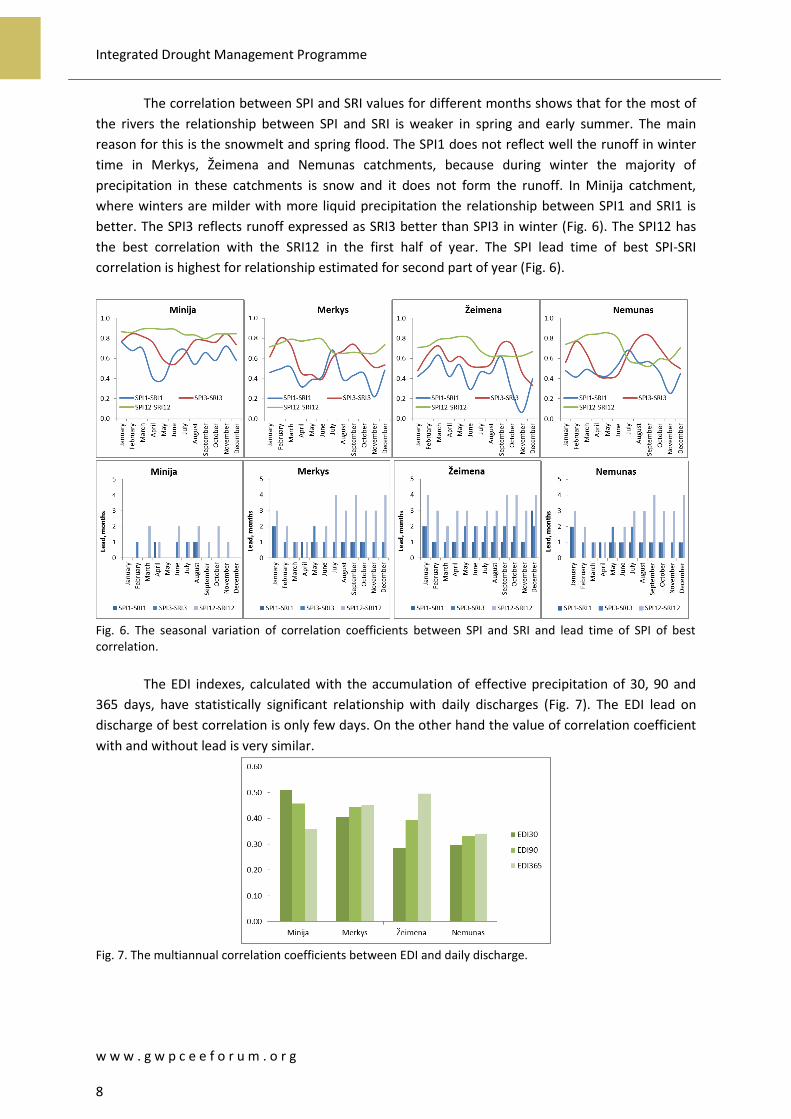
The correlation between SPI and SRI values for different months shows that for the most of
the rivers the relationship between SPI and SRI is weaker in spring and early summer. The main
reason for this is the snowmelt and spring flood. The SPI1 does not reflect well the runoff in winter
time in Merkys, Žeimena and Nemunas catchments, because during winter the majority of
precipitation in these catchments is snow and it does not form the runoff. In Minija catchment,
where winters are milder with more liquid precipitation the relationship between SPI1 and SRI1 is
better. The SPI3 reflects runoff expressed as SRI3 better than SPI3 in winter (Fig. 6). The SPI12 has
the best correlation with the SRI12 in the first half of year. The SPI lead time of best SPI-SRI
correlation is highest for relationship estimated for second part of year (Fig. 6).
Fig. 6. The seasonal variation of correlation coefficients between SPI and SRI and lead time of SPI of best correlation.
The EDI indexes, calculated with the accumulation of effective precipitation of 30, 90 and
365 days, have statistically significant relationship with daily discharges (Fig. 7). The EDI lead on
discharge of best correlation is only few days. On the other hand the value of correlation coefficient
with and without lead is very similar.
Fig. 7. The multiannual correlation coefficients between EDI and daily discharge.
Integrated Drought Management Programme
w w w . g w p c e e f o r u m . o r g 9
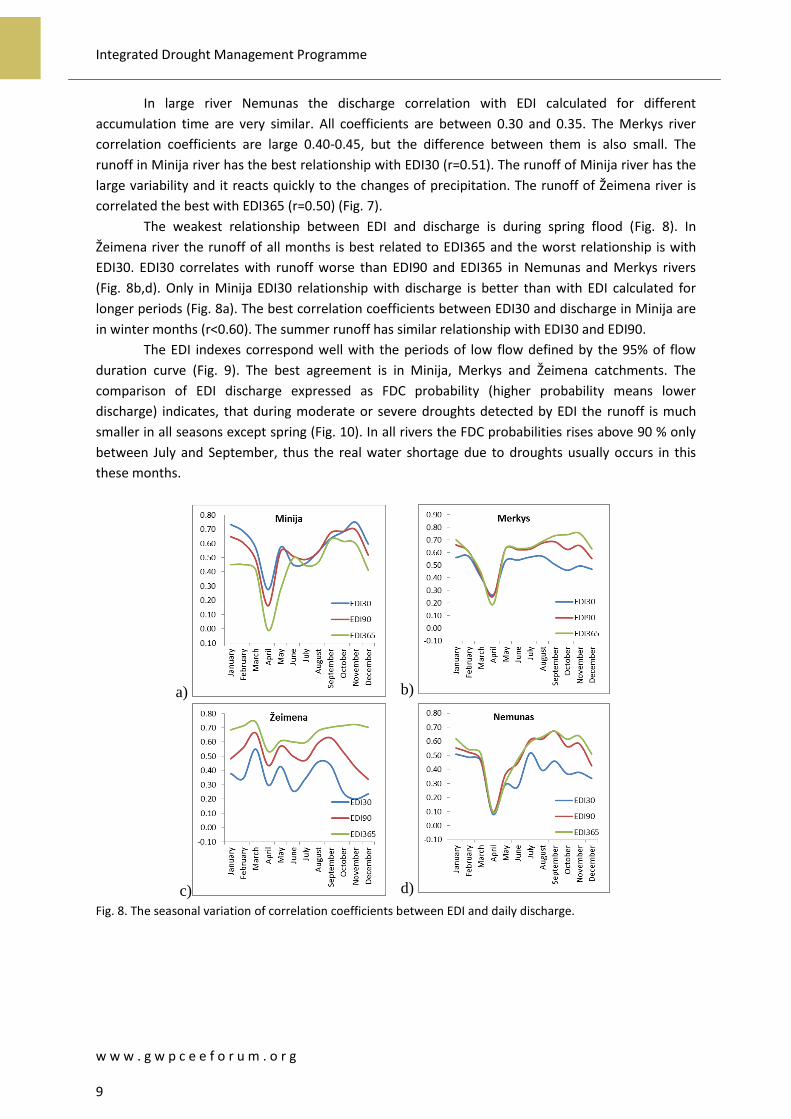
In large river Nemunas the discharge correlation with EDI calculated for different
accumulation time are very similar. All coefficients are between 0.30 and 0.35. The Merkys river
correlation coefficients are large 0.40-0.45, but the difference between them is also small. The
runoff in Minija river has the best relationship with EDI30 (r=0.51). The runoff of Minija river has the
large variability and it reacts quickly to the changes of precipitation. The runoff of Žeimena river is
correlated the best with EDI365 (r=0.50) (Fig. 7).
The weakest relationship between EDI and discharge is during spring flood (Fig. 8). In
Žeimena river the runoff of all months is best related to EDI365 and the worst relationship is with
EDI30. EDI30 correlates with runoff worse than EDI90 and EDI365 in Nemunas and Merkys rivers
(Fig. 8b,d). Only in Minija EDI30 relationship with discharge is better than with EDI calculated for
longer periods (Fig. 8a). The best correlation coefficients between EDI30 and discharge in Minija are
in winter months (r<0.60). The summer runoff has similar relationship with EDI30 and EDI90.
The EDI indexes correspond well with the periods of low flow defined by the 95% of flow
duration curve (Fig. 9). The best agreement is in Minija, Merkys and Žeimena catchments. The
comparison of EDI discharge expressed as FDC probability (higher probability means lower
discharge) indicates, that during moderate or severe droughts detected by EDI the runoff is much
smaller in all seasons except spring (Fig. 10). In all rivers the FDC probabilities rises above 90 % only
between July and September, thus the real water shortage due to droughts usually occurs in this
these months.
a) b)
c) d)
Fig. 8. The seasonal variation of correlation coefficients between EDI and daily discharge.

Integrated Drought Management Programme
w w w . g w p c e e f o r u m . o r g 10
Fig. 9. The dynamics of EDI indexes and periods with runoff lower than 95% FDC (red).
Fig. 10. Average discharge expressed as FDC probability (higher probability means lower discharge) during periods with EDI smaller than -1 (moderate and severe drought) and large then -1.
It can be concluded that:
The meteorological drought indexes SPI and EDI have statistically significant relationship with
hydrological drought indexes SRI and FI. The correlation between SPI and SRI is better with
indexes calculated using longer time steps. The correlation during spring is weakest due to runoff
formation from snowmelt.
The relationship between meteorological and hydrological drought indexes depends on the
properties of river catchment and climate. SPI and indexes calculated for shorter time steps
better represents the hydrological response in catchments where the water accumulation
capacity is smaller and where the part of surface and fast subsurface runoff in total river runoff is
large.
Moderate and severe drought periods identified by EDI usually coincide with the reduction off
runoff, but only during July-September the meteorological droughts may be related to water
resources shortage.

Integrated Drought Management Programme
w w w . g w p c e e f o r u m . o r g 11
2.2.2. Detecting hydrological drought in Poland
Values of SPI to SRI indices were used to developed a two-dimensional variable for drought
hazard assessment (Tokarczyk, Szalinska 2013). The proposed approach allows establishing five
classes of combined SPI-SRI variable which represents (Fig. 11): class 0 – normal meteorological and
hydrological conditions, class 1 – wet both meteorological and hydrological conditions, class 2 – dry
meteorological conditions and wet hydrological conditions, class 3 – dry both meteorological and
hydrological conditions, class 4 – wet meteorological conditions and dry hydrological conditions.
-4
-3
-2
-1
0
1
2
3
4
-4 -3 -2 -1 0 1 2 3 4
SRI
SPI
Międzylesie-Międzylesie
class 0 class 1 class 2 class 3 class 4 Fig.11. The SPI vs. SRI correlation plots for the coupled meteorological and hydrological stations for a) Nysa Klodzka and b) Prosna study basin.
With regard to drought formation, these classes can be interpreted in the following way.
Class 2 represents conditions in the first stage of drought - meteorological drought. Further shortage
of precipitation leads to a reduction in water resources and formation of hydrological drought (class
3). Restoring precipitation deficit may not be enough to instantly restore water resource. Therefore,
class 4 corresponds to the hydrological drought while meteorological conditions are at least back to
normal.
The obtained classification of hydro-meteorological conditions according to SPI-SRI indicator
was verified with the use of information derived from Nizowka model (Jakubowski&Radczuk, 2003,
Tallaksen, 2003). In the study Nizowka model was used to identify hydrological drought events
during the period 1966-2006 in Nysa Klodzka basin and provide their parameters i.e. drought
duration and deficit volume. These parameters were used to divide the identified hydrological
drought events into four categories: 1) droughts of low deficit volume and lasting less than 30 days,
2) droughts of low deficit volume and lasting more than 30 days, 3) droughts of big deficit volume
and lasting less than 30 days, 4) droughts of big deficit volume and lasting more than 30 days. This
discrimination between low and big deficit volume was done in reference to the median drought
deficit volume during the analyzed period. Each month was attributed with the SPI-SRI class and in
parallel with the category obtained with the use of Nizowka model. Category of the particular
drought event was assigned for all the months corresponding to the drought event. The coincidence
of a given SPI-SRI class and the adopted drought categorization was investigated by developing the
frequency distribution of a number of months belonging to each SPI-SRI class (0, 1, 2, 3, 4) from the
population of months categorized according to Nizowka model outputs. This verification procedure
was done for the subcatchment of the Odra River: Nysa Klodzka basin (Fig. 12).
The results indicate that for the months categorized as non-drought months according to
Nizowka model, the great majority (~70% - 90%) was in coincidence with SPI-SRI class 0, 1 or 2.

Integrated Drought Management Programme
w w w . g w p c e e f o r u m . o r g 12
Short drought periods (T<30 days) with low deficit volume were in coincidence with SPI-SRI class 0, 1
or 2 in 50% to 70%. Months with droughts of big deficit volume but short time duration were in
coincidence with SPI-SRI class 4 in 60% of the cases for Klodzko and Ladek Zdroj and in 33% in
Miedzylesie. In the latter locations there were many cases of droughts starting in the middle of
month what strongly influenced the results. Severe and long lasting droughts were mainly connected
with the months classified as SPI-SRI class 3. This was recognized for close to 50% of the cases for
Miedzylesie and more than 60 % of the cases for Klodzko and Ladek Zdroj.
0
10
20
30
40
50
60
70
80
90
100
class 0 class 1 class 2 class 3 class 4
fre
qu
ency
dis
trib
uti
on
[%]
NIZOWKA: lack of drought
Miedzylesie Klodzko Ladek Zdroj
0
10
20
30
40
50
60
70
80
90
100
class 0 class 1 class 2 class 3 class 4fr
eq
uen
cy d
istr
ibu
tio
n [%
]
NIZOWKA: low deficit volume and long duration
Miedzylesie Klodzko Ladek Zdroj
0
10
20
30
40
50
60
70
80
90
100
class 0 class 1 class 2 class 3 class 4
fre
qu
ency
dis
trib
uti
on
[%]
NIZOWKA: low deficit volume and short duration
Miedzylesie Klodzko Ladek Zdroj
0
10
20
30
40
50
60
70
80
90
100
class 0 class 1 class 2 class 3 class 4
fre
qu
ency
dis
trib
uti
on
[%]
NIZOWKA: big deficit volume and short duration
Miedzylesie Klodzko Ladek Zdroj
0
10
20
30
40
50
60
70
80
90
100
class 0 class 1 class 2 class 3 class 4
fre
qu
ency
dis
trib
uti
on
[%]
NIZOWKA: big deficit volume and long duration
Miedzylesie Klodzko Ladek Zdroj
Fig. 12 Frequency distribution of the % of months belonging to each SPI-SRI class from the population of months categorized according to NIZOWKA model outputs.
3. Drought hazard assessment The proposed methodology for drought hazard assessment is based on the probabilistic
assessment of the severity, duration and return time of drought estimated with the use of selected
drought indices. This assessment was done with the application of Markov chain models for the
study area of the Odra River (Poland). The detailed analysis were performed for three subbasins of
the Odra River: Nysa Klodzka, Bobr and Prosna (Tab. 4)
Tab.4 The physical-geographical characteristics of the investigated basins
River Gauging station
Basin area [km2]
Length of basin [km]
Max altitude
[m a.s.l.]
Min altitude
[m a.s.l.]
Net river density
[km/km2]
Afforestations [%]
Urbanization degree
[%]

Integrated Drought Management Programme
w w w . g w p c e e f o r u m . o r g 13
Nysa Klodzka
Bardo 1744 70,3 975 350 0,53 32 2,9
Bobr Jelenia Gora 5876
Prosna Bogusław 4280 185,0 280 97 0,38 20 2,7
Markov chain models (Cinlar, 1975) have been used for stochastic characterization of drought.
Gabriel and Neumann (1962) were among the first to apply Markov models for dry spell analysis.
Markov chains Lohani et al. (1998) forecasted drought conditions for future months, based on the
current drought class described by the Palmer index. Fernandez and Salas (1999) presented a
method for estimating the return period of droughts when underlying hydrological series (annual
streamflows) are autocorrelated. They assumed that the binary process consisting of dry years (D: Xt
< x0) and wet years (W: Xt ≥ x0) follows a simple (first order) Markov chain with two states (dry and
wet). Using the first-order Bayazit and Onoz (2005) analyzed the probability distribution and return
periods of joint droughts of a number of sites assuming that streamflows are cross-correlated first-
order Markov processes. Sharma and Panu (2012) applied Markov chain models as a simple tools for
predicting the T-year drought lengths based on annual, monthly and weekly SHI (standardized
hydrological index) sequences. They reported that that Markovchain-2 model was found satisfactory
on monthly and weekly time scale, as the river flows under consideration were strongly auto-
correlated.
Statistical characteristics of Markov chain provides information that can be used for drought
hazard assessment:
- probabilities of transition from one drought class to another, that represents proneness to
drought formation;
- return period of drought class which represent the probabilities of occurrence of the various
drought classes;
- expected residence time in drought class, which is the average time the process stays in a
particular drought class before migrating to another class and represents the duration of
that drought class;
- the expected first passage time from one class to another that represents the average time
period taken by the process to reach for the first time the given drought class starting from
some other class.
These characteristics (conditional probabilities, steady state probabilities, excepted residence
time and first passage time) were developed for the time series of long term SPI-SRI classes. The
stochastic process took one from the 5 possible stages in each month.
Tab.5 summarizes the obtained transition probabilities values for 3 subbasins of the Odra
River: Nysa Klodzka, Bobr and Prosna. Dominant transition probabilities (around 0.3) were
recognized for moving from normal, wet or meteorologically dry conditions (class 0, 1 and 2) to wet
conditions. The observed hydrological dry conditions (class 3 and class 4) result in a probability of its
continuation up to 44% - 48%. On the other hand, it is very unlikely to move from meteorological
and hydrological dry conditions (class 3) to normal, wet or only meteorological dry conditions in the
next month. Similarly, there is very low probability to move from these conditions (class 0, 1 or 3) to
solely hydrological dry conditions (class 4).
Tab.5. The empirical transition probabilities of moving from state i to j in next month for the selected subbasins of the Odra River

Integrated Drought Management Programme
w w w . g w p c e e f o r u m . o r g 14
Nysa Klodzka class 0 class 1 class 2 class 3 class 4
Current conditions
class 0 0.21 0.29 0.07 0.24 0.18
class 1 0.18 0.36 0.29 0.08 0.09
class 2 0.16 0.29 0.03 0.36 0.16
class 3 0.11 0.11 0.06 0.44 0.29
class 4 0.21 0.22 0.08 0.32 0.18
Bobr class 0 class 1 class 2 class 3 class 4
Current conditions
class 0 0.21 0.42 0.10 0.23 0.04
class 1 0.15 0.35 0.30 0.15 0.05
class 2 0.19 0.25 0.12 0.25 0.18
class 3 0.08 0.16 0.04 0.44 0.28
class 4 0.16 0.21 0.11 0.31 0.21
Prosna class 0 class 1 class 2 class 3 class 4
Current conditions
class 0 0.27 0.36 0.04 0.21 0.12
class 1 0.14 0.44 0.24 0.13 0.05
class 2 0.22 0.33 0.18 0.20 0.06
class 3 0.07 0.15 0.02 0.48 0.28
class 4 0.17 0.09 0.03 0.41 0.29
The values of steady-state probabilities were presented as a return period of each class
expressed in months (Fig. 13a). Class 3 and class 1 was found to be the most frequent one (every 3
and 4 months respectively), in all subbasins. It conforms that the same hydrological and
meteorological conditions are likely to occur within the same month.
The expected residence time represented the anticipated duration of belonging to each
class. The longest duration time (around 1.8 months) was established for class 3. Among analyzed
subbasins Prosna was found to have the longest residence time in each class (Fig. 13b).
a) b)
0
2
4
6
8
10
12
class 0 class 1 class 2 class 3 class 4
mo
nth
s
RETURN PERIOD
Bobr Nysa Klodzka Prosna
0 0.5 1 1.5 2
class 0
class 1
class 2
class 3
class 4
month
RESIDENCE TIME
Prosna Nysa Klodzka Bobr
Fig. 13 The return period [months] of each class developed for the locations in Nysa Klodzka and Prosna river basins Tab.6. The expected residence time of a given SPI-SRI class developed for the locations in Nysa Klodzka and Prosna river basins
The obtained values of the expected first passage of time were interpreted in terms of
seasonal variations of drought hazards formation, evolution and persistence. Drought hazard was
estimated from average time period (expressed in months) needed to move from one state to
another (Fig. 14a). Drought hazard formation was evaluated in terms of meteorological drought
hazard formation as the expected number of months required to move from wet conditions to
meteorological dry (1→2) and hydrological drought hazard formation as the expected number of
months required to move from normal conditions to ones (0→3). Hazard of drought evolution was
assessed as the expected number of months required to move from the state of exclusively

Integrated Drought Management Programme
w w w . g w p c e e f o r u m . o r g 15
meteorological dry conditions to hydrological dry conditions (2→3) and as the number of months
required to evolve to solely hydrological drought (3→4). Hazard of drought persistence was
evaluated as the expected number of months to pass from hydrological dry to normal or wet
conditions (3 or 4 → 0 or 1). All of the analyzed first passages of times were presented in the form of
radar plots summarizing the analyzed hazards. In order to keep the consistency of hazards direction,
the drought persistence of hazard was presented inversely.
The obtained results indicate that in Nysa Klodzka and Bobr there is a bigger hazard of
meteorological drought formation than in Prosna basin. Also in Nysa Klodzka and Bobr subbasin
there is a slightly bigger hazard of remaining in hydrological drought phase once the meteorological
drought is finished. On the other hand for Prosna River, it takes longer to move back from solely dry
conditions to normal or wet ones (Fig. 14b).
a)
0.0
2.0
4.0
6.0
8.0
10.0
12.0
t(1→2)
t(0→3)
t(2→3)
t(3→4)
12-t(3→0v1)
12-t(4→0v1)
low hazard: slow drought formation and evolution and short period of return to normal conditions
high hazard: fast drought formation and evolution and long period of return to normal conditions
haz
ard
of
dro
ugh
t p
ers
iste
nce
b)
0123456789
101112
t(1→2)
t(0→3)
t(2→3)
t(3→4)
12-t(3→0v1)
12-t(4→0v1)
Bobr Nysa Klodzka Prosna
Fig. 14. The interpretation of the developed first passage of times in terms of hazard of drought formation, evolution and persistence The radar plots of drought hazard developed for selected subbasins of the Odra River.
4. Drought hazard mapping Drought hazard can be defined by the frequency of occurrence of drought at various levels of
intensity and duration. The return period of a drought is related to the severity of the impacts
therefore provide vital information for drought risk management. Drought hazard mapping cater for
information on drought prone areas. It enables identification of the elements at the risk and
introduce mitigation measures adjusted to vulnerable areas.
Presentation of spatial distribution of drought hazard refers to the first phase of drought
formation caused by the lack of precipitation. Long-term datasets of one month SPI values
developed for the set of 87 meteorological stations located on the territory of Poland were used to
present various characteristics of drought hazard estimated with the application of Markov chain
model.
The behavior of SPI time series in selected sites was analyzed with Markovian model focusing
the transitions between drought categories (Paulo et al.2005). Markov chains were used in order to
estimate: (a) transition probabilities of different drought severity classes, (b) the expected time in
each class of severity, (c) the recurrence time to a particular drought class. Three drought severity
states, were considered: Non-drought (N), Moderate drought (1), Severe drought (2) and Extreme
Integrated Drought Management Programme
w w w . g w p c e e f o r u m . o r g 16
drought (3). The respective thresholds are those used by U.S. National Climatic Data Center, NOAA
(Tab.6).
Tab.6. Drought severity classes Cathegory of drought severity symbol SPI values
non-drought N > -0,5
moderate drought 1 [-0,5 ÷ -1,5)
severe drought 2 [-1,5 ÷ -2)
extreme drought 3 ≤ -2
For mapping of spatial extent of meteorological from point data, a Cressman interpolation
method was used. Cressman weights depend on the distance between the location where the value
of the field should be estimated and the location of the observation. This is a very simple and
numerically efficient method, however other interpolation techniques should be considered in order
to elaborate optimal interpolation method.
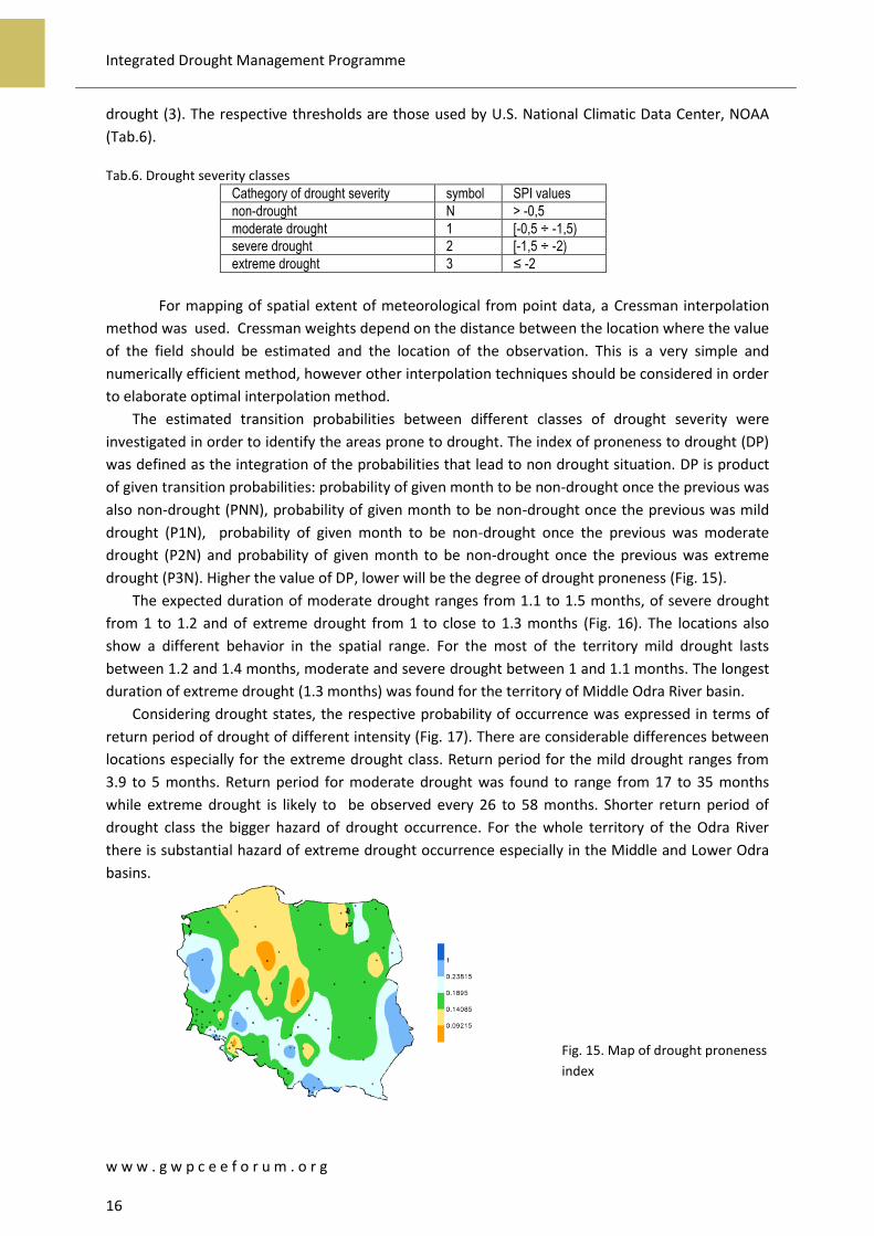
The estimated transition probabilities between different classes of drought severity were
investigated in order to identify the areas prone to drought. The index of proneness to drought (DP)
was defined as the integration of the probabilities that lead to non drought situation. DP is product
of given transition probabilities: probability of given month to be non-drought once the previous was
also non-drought (PNN), probability of given month to be non-drought once the previous was mild
drought (P1N), probability of given month to be non-drought once the previous was moderate
drought (P2N) and probability of given month to be non-drought once the previous was extreme
drought (P3N). Higher the value of DP, lower will be the degree of drought proneness (Fig. 15).
The expected duration of moderate drought ranges from 1.1 to 1.5 months, of severe drought
from 1 to 1.2 and of extreme drought from 1 to close to 1.3 months (Fig. 16). The locations also
show a different behavior in the spatial range. For the most of the territory mild drought lasts
between 1.2 and 1.4 months, moderate and severe drought between 1 and 1.1 months. The longest
duration of extreme drought (1.3 months) was found for the territory of Middle Odra River basin.
Considering drought states, the respective probability of occurrence was expressed in terms of
return period of drought of different intensity (Fig. 17). There are considerable differences between
locations especially for the extreme drought class. Return period for the mild drought ranges from
3.9 to 5 months. Return period for moderate drought was found to range from 17 to 35 months
while extreme drought is likely to be observed every 26 to 58 months. Shorter return period of
drought class the bigger hazard of drought occurrence. For the whole territory of the Odra River
there is substantial hazard of extreme drought occurrence especially in the Middle and Lower Odra
basins.
Fig. 15. Map of drought proneness
index

Integrated Drought Management Programme
w w w . g w p c e e f o r u m . o r g 17
a) expected residence time in moderate drought b) expected residence time in severe drought
c) expected residence time in extreme drought
Fig. 16. Map of expected residence time in given
drought severity
a) expected return period of moderate drought b) expected return period of severe drought
c) expected return period of extreme drought
Fig. 17. Map of expected return period for given
drought severity

Integrated Drought Management Programme
w w w . g w p c e e f o r u m . o r g 18
5. Conclusions Drought hazard assessment is the decisive information for effective management of risk.
Methodology for drought hazard mapping was developed with the use of selected drought indices.
The selection was done with the aim of their applicability in the country participating in the activity
5.4 (PO, LT, RO) as well as their relevance to the drought assessment in the sectors recognized as the
most vulnerable to drought: agriculture and water resources. The methodology concerned the
following issues:
Application scope. Development of hydro-information system that aimed to provide drought risk
information on operational basis requires operative drought indicators that uses the measurements
from standard monitoring network. Another challenge to support decision making in is the
development of the tools to combine multiple sources of information on drought and produce a
single marker of drought situation in relation to the geographical location. Real-time applications
promotes methods based on easily accessible meteorological and hydrological information. These
rationale can be meet with the use of indices. The relevance of given drought index for the particular
sector affected by drought have to be primary verified.
Temporal scale. Drought hazard assessment for different sectors vulnerable to drought may requires
different temporal resolution of drought indices. Therefore there is a need to look for a set of indices
that are capable to be run for the diverse periods in order to capture the significant variations of
meteorological and hydrological conditions.
Spatial scale. Drought risk have to be primary managed in the regional and local context. The local
scale is critical issue due to the heterogeneity in spatio-temporal hydro-meteorological variability
(Mishra and Singh, 2010). The applied methodology uses point data based on rain and stream
gauges in attempts to account for this heterogeneity. The hydrological variable represents the
behavior of a bigger territory (basin or subbasin) while meteorological variable is more local.
Standardized form of drought hazard assessment method allows for generation of maps across
different region.
Frequency analysis. Time series of the drought indices classes were investigated as a discrete-state,
discrete-time homogenous Markov chain. The analysis of the properties of Markov chain aimed to
evaluate the probability of transition between different classes, frequency of each class, residence
time in each class, time required to move from one class to another. These statistical characteristics,
derived for a basin scale, can be applicable to support decision making in the drought risk
management. The information on the proneness of a basin to drought formation, evolution and
persistence can be applied for drought risk mapping.
6. References Buitkuvienė M. S. (1998). Droughts in Lithuania. Scientific Report. Vilnius: LHMT, 403–427. (in Lithuanian, summary in English)
Dirsė A., Taparauskienė L. (2010). Humidity fluctuations in plant vegetation periods and a comparison of its assessment methods. Žemės ūkio mokslai, 17 (1-2), 9-17.
Gabriel, K.R., Neumann, J., 1962. A Markov chain model for daily rainfall occurrences at Tel Aviv. Quart. J. Roy. Meteorol. Soc. 88, 90–95.
Jakimavičiūtė N., Stankūnavičius G. (2008). An analysis of dry spells in Lithuania using different precipitation indices and classification techniques. Geografija. 44, 50–57. (in Lithuanian, summary in English)

Integrated Drought Management Programme
w w w . g w p c e e f o r u m . o r g 19
Jakubowski W., 2003. Guide and computer program NIZOWKA. Mathematic Division, Agricultural University, Wroclaw.Jakubowski W., Radczuk L., 2003, Estimation of Hydrological Drought Characteristics NIZOWKA 2003, http://www.geo.uio.no/edc/software/NIZOWKA/Software_Manual_NIZOWKA.pdf
Kim D.W., Byun H.R., and Choi K.S. (2009). Evaluation, modification and application of the Effective Drought Index to 200-year drought climatology of Seoul, Korea. Journal of Hydrology, 378, 1 – 12.
Lithuanian Ministry of Environment (2002). Annual Report 2002. Vilnius
Lohani, V.K., Loganathan, G.V., 1997. An early warning system for drought management using the palmer drought index. J. Am. Water Resour. Assoc. 33 (6), 1375–1386.
M. Bayazit & B.Önöz (2005): Probabilities and return periods of multisite droughts, Hydrological Sciences Journal, 50:4, -615
Paulo, A.A., Ferreira, E., Coelho, C., Pereira, L.S., 2005. Drought class transition analysis through Markov and Loglinear models, an approach to early warning. Agric. Water Manage. 77, 59–81.
Paulo, A.A., Pereira, L.S., 2007. Prediction of SPI drought class transitions using Markov chains. Water Resour. Manage. doi:10.1007/s11269-006-9129-9.
Schubert S., Wang H., Suarez M. (2011). Warm season subseasonal variability and climate extremes in the Northern Hemisphere: The role of stationary Rossby waves. J. Climate, 24, 4773–4792.
Sharma T.C., Panu U.S., 2012, Prediction of hydrological droughts based on Markov chains: case of the Canadian prairies, Hydrological Sciences Journal, 57:4, 705-722
Vasiliades, L., A. Loukas, and N. Liberis, 2010: A water balance derived drought index for Pinios River Basin, Greece. Water Resources Management, 25, 1087-1101
Tallaksen L.M., 2003: Background Information NIZOWKA, http://www.geo.uio.no/edc/software/NIZOWKA/Background_Information_NIZOWKA.pdf
Taparauskienė L., Lukševičiūtė A., Maziliauskas A. (2013). Comparison of Standardized precipitation and Selyaninov hydrothermal drought indices. In Rural Development 2013 (Ed. In chief Atkočiūnienė V.) Proceedings of the sixth international scientific conference. vol. 6 (3), 486-489.
Tokarczyk T., Szalińska W., 2010. Operacyjny system oceny zagrożenia suszą, W: Hydrologia w Inżynierii i Gospodarce Wodnej, t. I. pod red. B. Więzika. Wyd. PAN Komitet Inżynierii Środowiska, Seria: Monografie Nr 68, Warszawa, s. 285-294.
Tokarczyk T., Szalińska W., 2013 a. Combined analysis of precipitation and water deficit for drought hazard assessment. Hydrological Sciences Journal, DOI: 10.1080/02626667.2013.862335.
Tokarczyk T., Szalińska W., 2013 b. The operational drought hazard assessment scheme – performance and preliminary results. Archives of Environmental Protection. in press, ISSN (Online) 2083-4810, ISSN (Print) 2083-4772
Valiukas D. (2011). Dry periods in Vilnius in 1891-2010. Geografija. 1, 9-18. (in Lithuanian, summary in English)