Embed Size (px)
Citation preview
Silvya Dewi Rahmawati
Integrated Field Modeling and Optimization Thesis for the degree of philosophiae doctor Trondheim, March 2012 Norwegian University of Science and Technology Faculty of Information Technology, Mathematics and Electrical Engineering Department of Engineering Cybernetics
ii
Summary
Oil and gas continue to be widely used worldwide as energy resources, because new sources of safe energy have not yet been well developed. These conditions have motivated researchers in the area of oil and gas production to investigate new approaches to the application of optimization methods to maximize gas or oil production rates and to minimize production costs.
This PhD research investigates production optimization of conventional and unconventional reservoirs by considering compositional and black-oil reservoir fluid properties and presents economic evaluation in terms of a net present value (NPV) formulation. In general, unconventional reservoirs are characterized by large volumes that are difficult to develop since the permeability is low (<0.1 mD). A new approach to NPV calculation is introduced in which NPV is taken as the maximum cumulative NPV and not always the value at the end of the simulation. The maximum cumulative NPV has correlation with optimum field operation time using current production and/or injection strategy. The proposed method provides an advantage in determining when a new production strategy and/or management decision should be applied after the optimum field operation time is reached.
Three new approaches related to oil and gas production performance will be presented in this thesis: (i) a cyclic shut-in strategy for liquid-loading gas wells, (ii) production optimization using an integrated model from subsurface to surface facilities, which is then linked to an economic analysis, and (iii) an optimal injection strategy for oil reservoirs when water and gas injection are available. A framework for decision support tools, based on available software, is implemented and a derivative-free optimization method, the Nelder-Mead Simplex, is applied.
A cyclic shut-in strategy for liquid-loading gas wells in unconventional gas reservoirs has been studied. An unconventional reservoir is a potential future energy resource offered by new methods of exploration and production. One of the characteristics of an unconventional gas reservoir is low permeability, in which a gas well producing reservoir fluids usually experiences a liquid-loading condition during production. This condition is caused by accumulation of liquid at the bottom of the well, where an increasing liquid column in the well results in hydrostatic back-pressure to the reservoir, destabilizing the multiphase flow in the well, decreasing the gas production rate, and finally killing the well. A cyclic shut-in strategy is introduced to reduce the loss of gas production by increasing the reservoir pressure and gas production thereby will able to push the liquid column up to the surface. The simulation results show consistently that ultimate recovery increases, for both vertical and horizontal fractured wells.
iii
An integrated field model and optimization may play an important role during production because an integrated model may produce comprehensive operational recommendations. An integrated field model combined with optimization presents many technological challenges in terms efficient algorithms to couple models, as well as models with optimization, and sufficient hardware capability to run the complex model. A benchmark case which consists of three different reservoirs that are linked to a surface facility model has been developed. The surface process model interacts with the three reservoir models through the distribution of available produced gas for reinjection into the three reservoirs. The reservoir and surface process variables are optimized in terms of maximizing asset value. The integrated model and corresponding optimization results provide a benchmark that contributes to academic and industrial knowledge on the potential value of joint optimization of the upstream and downstream parts of the production chain. The benchmark should be valuable as a tool for assessing future alternative methods for production chain optimization.
An optimal injection strategy for miscible water alternating gas injection is presented as a mixed-integer non-linear problem formulation. A heuristic approach is chosen to solve the problem. The injection strategies include gas injection, water injection, WAG, and a combination of the above injection strategies. The injection strategies are optimized to find the best injection strategy for a particular reservoir. The optimization was conducted for two production strategies: artificial lift and natural flow. The study concluded that a gas-water injection strategy with long-time gas injection and artificial lift was the best scenario for the example used in this study. The artificial lift economic value was significantly better than natural flow optimization scenarios, with an NPV increase of 8 − 31%. Moreover, the injection optimization method presented in this study should have significance potential for other miscible oil reservoirs.
iv
Acknowledgments
A study of optimization in oil and gas production conducted in collaboration between the Cybernetics Engineering Department and the Department of Petroleum Engineering and Applied Geophysics, NTNU, Trondheim, Norway, is reported in this PhD thesis. Many people participated in various ways to ensure that my research succeeded, and I am thankful to all of them. Unfortunately, not everyone could be mentioned here, but I would like to use this opportunity to express my deepest gratitude for those who deserve special recognition.
First, I would like to thank my supervisor, Professor Bjarne A. Foss, for the opportunity given to me as his student. He has contributed valuable comments, interesting discussions, and comprehensive feedback during this study.
I would like to thank my co-supervisor, Professor Curtis Hays Whitson, for bringing me into the deep and detailed field of petroleum research. His research ideas, patience, and courage made it possible to complete this thesis. I am thankful for other assistance he provided such as introducing me to other petroleum researchers in PERA/Petrostreamz Company and Norman, Oklahoma.
My appreciation also goes to Professor Michael Golan, Professor Ken Starling, and Mr. Bob Hubard for valuable discussions during my stay in Norman, Oklahoma, USA, while working on the integrated modeling and optimization. I would like to acknowledge the IO Center, NTNU, Trondheim, Norway, for the financial support.
I also would like to thank PERA/Petrostreamz employees Arif Kuntadi, Faizul Hoda, and Aleksander Juell for offering an efficient way to learn about oil and gas simulators and for valuable discussions and software assistance.
Further, I would like to thank to all of my colleagues at the Cybernetics Engineering Department; Hardy B. Siahaan, Milan Milovanovic, Eka Suwartadi, Vidar Gunnerud, Brage Knudsen, Agus Hasan and Lei Zhou for a friendly and lively work environment and discussions about my research; and Tove Johnsen, Bente Lindquist, and Eva Amdahl for the useful information and assistance about courses and travel. Special thanks go to the Indonesian community in Trondheim for the activities and creativities that make me feel like home during my stay in Trondheim.
Finally, I am eternally indebted to my family and my husband, Ardiyan Harimawan, for their unconditional love and understanding, which enabled me to complete my research. A special thank you goes to my mother, Suntari Munir, and my father, Syamsul Munir, for always supporting me in every way.
Trondheim, November 2011 Silvya Dewi Rahmawati
v
Table of Contents Summary ....................................................................................................................................... ii
Acknowledgments ...................................................................................................................... iv
Table of Contents .......................................................................................................................... v
Abbreviations ............................................................................................................................. viii
Chapter 1 General Introduction ................................................................................................. 9
1.1 Background ................................................................................................................... 9
1.2 Motivations and Problem Formulations ................................................................. 10
1.3 Software Simulation Overview ................................................................................ 12
1.4 Contributions .............................................................................................................. 14
1.5 Thesis Outline ............................................................................................................. 16
1.6 List of publications ..................................................................................................... 16
1.7 List of presentations ................................................................................................... 17
Chapter 2 Cyclic Shut-In Strategy for Liquid-Loading Gas Wells ...................................... 18
2.1. Introduction ..................................................................................................................... 18
2.2. Model Observations ........................................................................................................ 20
2.3. Cyclic Shut-in Strategy for Vertical Wells .................................................................... 22
2.4. Cyclic Shut-in Strategy for Horizontal Wells .............................................................. 27
2.5. Discussion and Conclusion ............................................................................................ 34
Chapter 3 Integrated Field Modeling and Optimization Benchmark ................................. 38
3.1. Introduction ..................................................................................................................... 38
3.1.1. Background ............................................................................................................... 38
3.1.2. Motivation ................................................................................................................. 40
3.2. Model Overview .............................................................................................................. 41
3.2.1. Reservoir Model ....................................................................................................... 41
3.2.2. Well Vertical-Flow Models ..................................................................................... 45
3.2.3. Surface-Pipeline Models .......................................................................................... 48
3.2.4. Surface Process Model ............................................................................................. 50
3.2.5 Thermodynamic Model ............................................................................................ 52
3.2.6. Economic Model ....................................................................................................... 53
vi
3.3. Model Integration and Software Applications ............................................................ 55
3.3.1. Model Integration ..................................................................................................... 55
3.3.2. Software Application ............................................................................................... 56
3.4. Base-Case Description .................................................................................................... 60
3.5 Sensitivity Analysis .......................................................................................................... 62
3.5.1. Sensitivity Analysis for Project Time Step ............................................................ 63
3.5.2. Sensitivity Analysis for Operational Parameters ................................................. 69
3.6. Optimization .................................................................................................................... 75
3.7. Conclusion ........................................................................................................................ 77
Chapter 4 A Mixed-Integer Non Linear Problem Formulation for Miscible WAG Injection ....................................................................................................................................... 79
4.1. Introduction ..................................................................................................................... 79
4.2. Problem Formulation ...................................................................................................... 81
4.2.1. Injection Scenarios .................................................................................................... 81
4.2.2. Economic Model ....................................................................................................... 82
4.2.3. Reservoir Description .............................................................................................. 83
4.2.4. Optimization Problem ............................................................................................. 83
4.2.5. Solution Approach ................................................................................................... 86
4.3. Study Case ........................................................................................................................ 87
4.3.1. Single-Well Producer and Injector Case ................................................................ 88
4.3.2. Multi-Well Producers and Injectors Case ............................................................. 88
4.4. Optimization Results ...................................................................................................... 90
4.4.1. Single-Well Case with Natural Flow Production Method .................................. 90
4.4.2. Single-Well Case with Artificial Lift Production Method .................................. 97
4.4.3. Multi-Well Case with Natural Flow Production Method ................................. 104
4.4.4. Multi-Well Case with Artificial Lift Production Method ................................. 114
4.4.5 Simulation Summary .............................................................................................. 125
4.5 Discussion ........................................................................................................................ 126
4.5.1 Oil Recovery Analysis ............................................................................................. 126
4.5.2 Geological Uncertainty Analysis ........................................................................... 133
4.5.3 WAG and GAW Analysis ...................................................................................... 137
4.6 Conclusion ....................................................................................................................... 141

vii
Chapter 5 Summary and Suggestions for Future Work ..................................................... 143
Nomenclature ........................................................................................................................... 146
References .................................................................................................................................. 150
Appendix A ............................................................................................................................... 156
viii
Abbreviations
BHP Bottomhole Pressure.
CM Case Matrix
DPC Dew Point Controller.
EOS Equation of State.
GAW Gas Alternating Water
GI Gas Injection
GOR Gas Oil Ratio.
GLR Gas Liquid Ratio.
OGR Oil Gas Ratio.
OLE Object Linking and Embedding.
OPEX Operational Expenses.
LGR Liquid Gas Ratio.
MFHW Multi-Fracture Horizontal Well
MINLP Mixed-Integer Non Linear Programming.
NGL Natural Gas Liquids.
NPV Net Present Value.
PTS Project Time Step.
PVT Pressure/Volume/Temperature
THP Tubing Head Pressure.
WAG Water Alternating Gas.
WI Water Injection
WOR Water Oil Ratio.
9
Chapter 1
General Introduction
This thesis begins with a description of the research background, motivation, and problem formulation for this PhD project. Software tools and optimization methods are explained in subsection 3, followed by a description of the project contributions to the petroleum research. An outline of the thesis, a list of publications and presentations are presented at the end of this chapter.
1.1 Background
The optimization of petroleum production is an interesting approach to meet increasing world energy demands and reduce production costs. According to Hart Energy, the U.S. Energy information administration, and the International Energy Agency, worldwide oil demand in 2011 was 89 million barrels per day. A worldwide demand for 99 million barrels of oil per day is expected by 2035 and a 44% increase in the demand for natural gas is predicted from the year 2008 till 20351
Fig. 1-1. Historically, most
oil and gas production is from conventional reservoirs (resource triangle, ). Conventional oil or gas reservoir is typically “free gas or free oil” trapped in porous zones in various natural rock formations such as carbonates, sandstones, and siltstones. Production of oil and gas from these reservoirs is easy, but their volumes are limited.
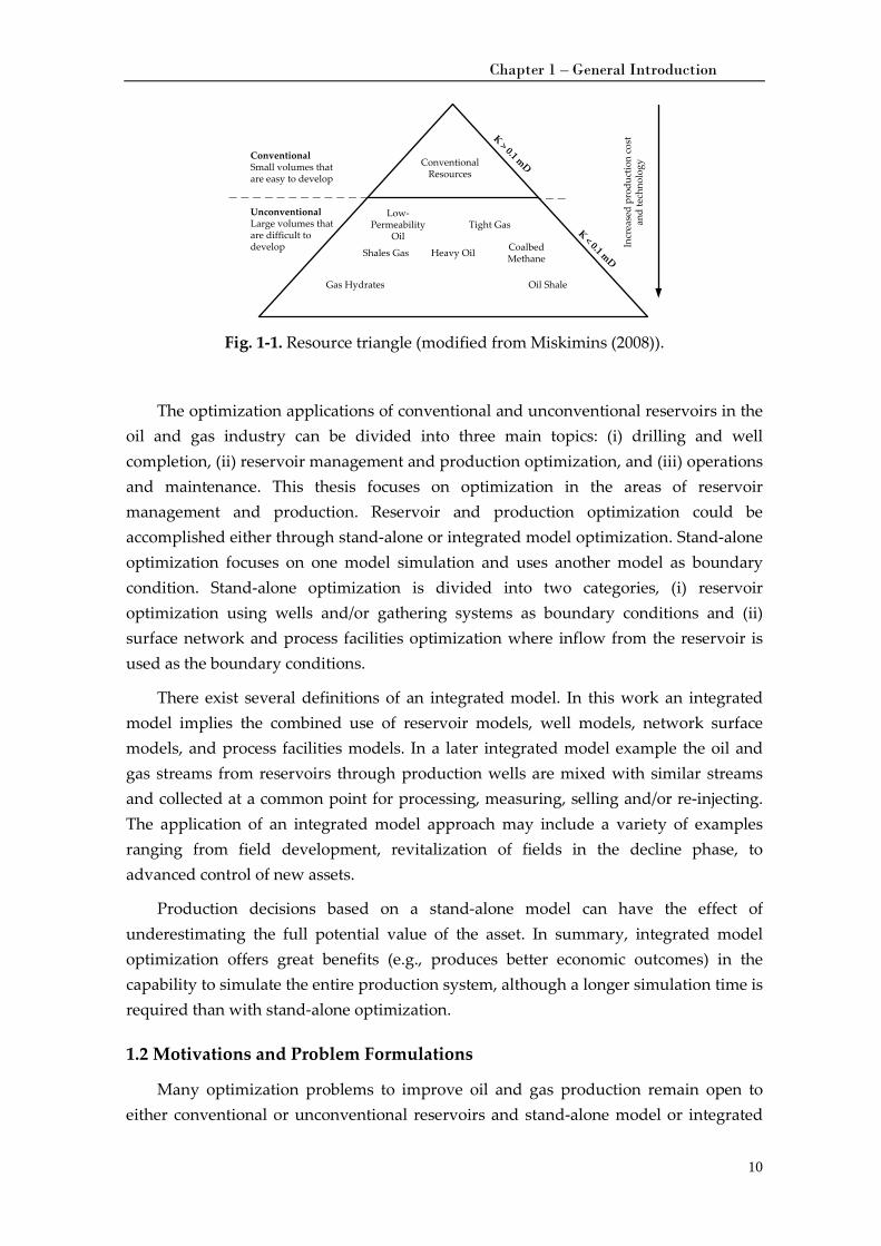
Currently, interest is shifting to the exploration and production of unconventional reservoirs. Those reservoirs have larger volumes, but are more challenging for the production of oil and gas. Unconventional reservoirs have been defined as formations that cannot be produced at economic flow rates or that do not produce economic volumes of oil and gas without stimulation treatments or special recovery processes and technologies (Miskimins (2008)). The technological improvements in horizontal drilling and fracturing have made unconventional resources commercially viable and have revolutionized worldwide oil and natural gas supply. Examples of unconventional reservoirs include heavy oil (extra heavy oil), oil sands, oil shales, tight gas and gas shales.
1 Source was taken from TIME magazine April 11, 2011
Chapter 1 – General Introduction
10
Fig. 1-1. Resource triangle (modified from Miskimins (2008)).
The optimization applications of conventional and unconventional reservoirs in the oil and gas industry can be divided into three main topics: (i) drilling and well completion, (ii) reservoir management and production optimization, and (iii) operations and maintenance. This thesis focuses on optimization in the areas of reservoir management and production. Reservoir and production optimization could be accomplished either through stand-alone or integrated model optimization. Stand-alone optimization focuses on one model simulation and uses another model as boundary condition. Stand-alone optimization is divided into two categories, (i) reservoir optimization using wells and/or gathering systems as boundary conditions and (ii) surface network and process facilities optimization where inflow from the reservoir is used as the boundary conditions.
There exist several definitions of an integrated model. In this work an integrated model implies the combined use of reservoir models, well models, network surface models, and process facilities models. In a later integrated model example the oil and gas streams from reservoirs through production wells are mixed with similar streams and collected at a common point for processing, measuring, selling and/or re-injecting. The application of an integrated model approach may include a variety of examples ranging from field development, revitalization of fields in the decline phase, to advanced control of new assets.
Production decisions based on a stand-alone model can have the effect of underestimating the full potential value of the asset. In summary, integrated model optimization offers great benefits (e.g., produces better economic outcomes) in the capability to simulate the entire production system, although a longer simulation time is required than with stand-alone optimization.
1.2 Motivations and Problem Formulations
Many optimization problems to improve oil and gas production remain open to either conventional or unconventional reservoirs and stand-alone model or integrated
Conventional Resources
Low-Permeability
OilTight Gas
Shales Gas Heavy Oil Coalbed Methane
Gas Hydrates Oil Shale
ConventionalSmall volumes that are easy to develop
UnconventionalLarge volumes that are difficult to develop
K < 0.1 mD
K > 0.1 mD
Incr
ease
d pr
oduc
tion
cost
an
d te
chno
logy
Chapter 1 – General Introduction
11
models. The motivations and problem formulations for this PhD study are categorized into three topics: (i) a cyclic shut-in strategy for liquid-loading gas wells, (ii) integrated field modeling and optimization, and (iii) optimal injection strategy for oil reservoirs when water and gas injection are available in the surface. Descriptions of these topics are as follows:
(i) Cyclic shut-in strategy for liquid-loading gas wells.
A common problem during gas production is that the occurrence of liquid-loading, especially for unconventional (low-permeability) gas reservoirs, has a huge impact on gas production. Liquid-loading occurs as a result of the gas velocity is not high enough to carry the liquid or water to the surface. Lea and Nickens (2004) summarized several technologies to solve the liquid-loading problem that are commonly used by industry: (i) sizing production strings (a properly designed smaller tubing or velocity string), (ii) installing a compressor, (iii) plunger lift, (iv) pumping (beam pumping and hydraulic pumping), (v) foaming, and (vi) gas lift. All of the currently available technologies to solve liquid-loading use external or additional sources and therefore add to operating cost. A new idea is introduced in this study to increase gas velocity immediately after the onset of liquid-loading by using the reservoir capability (reservoir pressure) that does not require external technology that would add economic cost.
(ii) Integrated Field Modeling and Optimization.
Integrated field modeling and optimization has a significant potential in the petroleum industry, particularly for field development and continuous asset-management evaluation. The interdependence between reservoir, surface pipeline network, process facilities, and economic analyses are observed simultaneously. The integrated field model helps to determine some specific problems that are undetectable using stand-alone model simulation (e.g., flow-assurance problem during CO2 injection (Galic et al. (2009))). This topic suggests an approach to understanding the oil and gas production dynamics from the reservoir to the surface processes in terms of an integrated model and optimization. The case study is developed from three reservoirs (i.e. lean-gas condensate, rich-gas condensate, and oil reservoirs), a surface facility process, and a simplified economic model. The model is tightly coupled due to gas injection distributions from the surface facility to the three reservoirs. Optimization is conducted to maximize field economics.
(iii) Optimal Injection Strategy for Oil Reservoirs.
An optimal injection strategy has been studied intensively for oil reservoirs when water and gas injection are available. Research results on optimal water alternating gas (WAG) injection strategies have been implemented in many oil
Chapter 1 – General Introduction
12
and gas fields around the world, but there is still much room for improvements by applying optimization methodology. Christensen et al. (2001) have reviewed about 60 fields under WAG and WAG optimization around the world. In this PhD study, the motivation was to develop an optimization formulation for oil reservoirs when there is water and gas injection available that allows the water-gas cyclic injection process for convergence to several operational solutions far from “traditional” short-cycle WAG strategies.
1.3 Software Simulation Overview
The main tools used in this research are presented as software platforms. Reservoir simulations are conducted using SENSOR®, surface process simulation using HYSYS®, and pressure drop calculation using PROSPER®. All simulations are run through the software platform, Pipe-It®. All of the optimization problems are solved using derivative-free optimization based on a constrained Nelder-Mead Simplex algorithm Pipe-It’s default solver. General descriptions of the software simulations are given below.
SENSOR Reservoir Simulator®
The SENSOR reservoir simulator was developed by Coats Engineering, Inc., and is applicable for compositional and black oil fluid types (Sensor Reference Manual (2009)). Compositional and black oil reservoir simulations were presented in this thesis. The compositional simulations were conducted in two chapters; an integrated model and optimization (Chapter 3) and optimal injection strategy for oil reservoirs (Chapter 4). A black oil fluid type simulation was presented in the liquid-loading gas wells (Chapter 2). The SENSOR reservoir simulator was the preferable choice to perform those simulations because it provides benefits in terms of speed, accuracy, stability, and reliability.
Aspen HYSYS®
The HYSYS simulator, developed by Aspen Technology, Inc., was used to simulate the surface facilities (Aspen HYSYS User Guide (2004)). HYSYS is considered to be one of the leading software packages of integrated simulation environments available to the downstream process industries. HYSYS supports several integration techniques and is completely Object Linking and Embedding (OLE) compliant.
Petex - PROSPER®
The PROSPER simulator, developed by Petroleum Experts, is a well performance design program for modeling tubing and pipeline in oil and gas fields (Petroleum Experts (IPM Tutorials) (2004)). PROSPER provides the ability to predict tubing and pipeline hydraulics and temperatures with accuracy and speed. The following well
Chapter 1 – General Introduction
13
types can be simulated using PROSPER: (i) gas, oil, water, and condensate production wells, (ii) water and steam injection wells, (iii) naturally flowing, (iv) artificial lifted, (iv) multi-layer and multi-lateral, and (v) deviated and horizontal wells.
Petrostreamz Pipe-It®
Petrostreamz Pipe-It is used as a software platform and optimizer for all issues addressed in this thesis. Manual data transfer between simulators, as conventionally practiced, was avoided. Pipe-it has the ability to maintain a detailed, quantitative upstream-to-downstream accounting of the individual models that constitute petroleum resources information. This software bridges the work of reservoir engineers, who speak in terms of volumetric rates, with process engineers, who often speak in terms of component molar rates, and ultimately with managers, who speak in terms of currency, revenue, net present value (NPV) and profit (Pipe-It Online Documentation, 2006). Pipe-It allows access to measured data provided by online metering and spot testing stored in databases. Pipe-it includes the Streamz “engine”, which allows translation of measured and calculated streams from one characterization to others, as needed by downstream model in an integrated system. Streamz can also be used as a surface separation process simulation similar to HYSYS, but without heat and energy balance. Pipe-It is linked to an optimization routine based on the constrained Nelder-Mead Simplex algorithm.
Nelder-Mead Simplex Algorithm Because of the nonlinearity of the system, petroleum production optimization
problems are characterized by a non-convex objective function. Derivative information may be expensive to obtain or nonexistent. The suitable optimization method for this type of problem is therefore a derivative-free method. Among the derivative-free optimization methods, Nelder-Mead Simplex (Nelder and Mead (1965) and Lagarias et al. (1998)) is chosen to search for the optimum solution in the optimization problems discussed in this study because the application of this method in the three topics is still new and because its performance in handling problems is acceptable.
Nocedal and Wright (2006) explain how this algorithm seeks to remove the vertex in the decision space with the worst objective function value and replace it with another point with a better value. The new point is obtained by reflecting, expanding or contracting the simplex along the line that joins the worst vertex with the centroid of the remaining vertices. If the algorithm cannot find a better point in this manner, the algorithm retains only the vertex with the best function evaluation, and the algorithm then shrinks the simplex by moving all other vertices toward this value. The convergence criteria used in the optimization method are related to the improvement of the objective function and the change in the decision variable from one iteration point to the next.
Chapter 1 – General Introduction
14
1.4 Contributions
The contributions of this thesis are divided into three categories based on topics addressed: (i) a cyclic shut-in strategy for liquid-loading gas wells, (ii) integrated field modeling and optimization, and (iii) optimal injection strategy for oil reservoirs. In general, topic (i) is focused on finding new technology or approaches to solve the liquid-loading problem, and topics (ii) and (iii) are focused on optimization, that is maximizes the economic model (NPV) for different cases and implementations. The NPV approach used in this study is unique in that the NPV value is the maximum of the cumulative NPV and not the NPV at the end of the simulation time. The time when cumulative NPV reaches maximum value provides important information for the field operation. This value means that beginning from day 1 until the maximum cumulative NPV is reached, it is profitable to implement the existing production and injection strategy. After the maximum cumulative NPV has been reached, another field policy, including production and injection strategies, should be changed to obtain higher field revenue and lower production cost. The description of the research contributions for each addressed topic are presented next.
(i) Cyclic Shut-in Strategy for Liquid-Loading Gas Wells
The goal for this research is to show that using reservoir pressure increments can increase gas velocity during liquid-loading problems in gas wells. The reservoir pressure is increased using a cyclic shut-in method, which is applied immediately after the onset of liquid-loading. The implementation is tested for fractured vertical and horizontal well models for different permeability values. The cyclic shut-in strategy shows improvement in ultimate gas recovery.
(ii) Integrated Field Modeling and Optimization
The integrated field modeling study has produced a benchmark case that can be used to show how potential reservoir production sharing occurs as a result of changes that may happen during production such as the introduction of a new production strategy. The integrated model consists of reservoir models including well models, a surface process facility including surface pipeline models and an economic model. The simulators of the different models use different data structures, time scales, standards, and the transfer of information between the simulators compromises the quality of information has been shown to be maintained. Transfer of data is dynamically linked between all of the model components.
This research project provides studies of reservoir and surface commercial software coupled to develop and implement an integrated field model simulation and optimization. No proxy models were used. The production system is essentially a flow system fed by the reservoir at one end and the exit of product streams at the other end. There is a feedback flow from the surface facility to the reservoirs in terms of gas
Chapter 1 – General Introduction
15
injection distribution. The surface process model is a steady state model, while the reservoirs are dynamic models. The starting point of this work was a gas-cycling benchmark presented by Juell et al. (2010).
The production performance from the three reservoirs are evaluated and optimized. The optimization has been conducted on the field level, from the reservoir to the process facility system. Conceptual field development studies require the assessment of large numbers of design parameters that constitute a field development plan. Identifying, screening, assessing and ranking crucial field optimization variables were chosen by performing sensitivity analyses for the global system to evaluate which variables have the greatest influence on the system. The objective of the optimization problem is maximizing NPV and the optimization method used is the Nelder-Mead Simplex. The complete benchmark description is available through a portal at the IO center web-pages (http://www.ipt.ntnu.no/~io-opt/wiki/doku.php).
(iii) Optimal Injection Strategy for Oil Reservoirs
The goal for this study is to develop a systematic formulation to determine the best injection strategy when water and gas injection is available. The injection strategy varies among single-cycle water-gas injection, multi-cycle water alternating gas injection, continuous water or gas injection, or a combination of all of these strategies. Decision variables play an important role such as, injection volumes, injection pressures and the time to change from one optimization strategy to another. The optimization has the objective to maximize NPV and the optimization results are produced by the Nelder-Mead Simplex method.
Single-well and multi-well production and injection cases with two different production strategies (natural flow and artificial lift) are used to test the optimization problem. Different initial values are tested to find the best injection strategy and the best injection operating conditions. The simulation results show that the optimum NPV indeed depends on the initial value. Optimization for multi-well cases is conducted in two steps: (i) the injection wells are assumed to have the same injection operating conditions, and (ii) the injection wells are assumed to have different operating conditions. The optimization using the same injection operating conditions provides “good” initial values for the optimization using different operating conditions, and the strategy helps to achieve convergence faster, reduce the CPU time, and define the robustness in terms of initial value. Geological uncertainty analyses are included only for the single-well model with an artificial lift production strategy in the discussion to verify the best injection strategy.
Moreover, optimization implementation in those three topics is a research activity and can therefore both benefit from and contribute to the ongoing research in the field of derivative-free optimization and petroleum production.
Chapter 1 – General Introduction
16
1.5 Thesis Outline
The remainder of the thesis is presented in four chapters, as described below: • Chapter 2: Cyclic Shut-in Strategy for Liquid-Loading Gas Wells. A cyclic
shut-in strategy is implemented for liquid-loading gas wells. The liquid-loading is assumed to occur when the gas production is below a certain value. The shut-in strategy is implemented for fractured vertical and horizontal wells with different shut-in times. In each vertical and horizontal well case there are three production strategies that are compared. First is a production strategy where shut-in method is applied to the well immediately after liquid-loading occurs. Second is a production strategy where the well never has a liquid-loading problem, and third is a strategy where the well has a liquid-loading problem but continues to produce with the average metastable rate.
• Chapter 3: Integrated Field modeling and Optimization Benchmark. A stable integrated model benchmark case is developed from reservoir through surface process facility models, including an economic model. Key parameters in the integrated system are examined through sensitivity analyses, and optimization is performed using the Nelder-Mead Simplex method.
• Chapter 4: A Mixed-Integer Non Linear Problem Formulation for Miscible WAG Injection. A systematic optimization approach to determine the best injection strategy and the best injection operating conditions is formulated. The optimization problem is tested for the cases of single-well and multi-well production and injection wells. Two production strategies are used, natural flow and artificial lift. Geological uncertainty is analyzed with the example of single-well production and injection wells under artificial lift. The optimization method is the Nelder-Mead Simplex method.
• Chapter 5: Summary and Suggestions for Future Work.
1.6 List of publications
• Rahmawati, S.D., Whitson, C.H., Foss, B. and Kuntadi, A. “Multi-Filed Asset Integrated Optimization Benchmark”. Paper SPE 130768 presented at the SPE EUROPEC/EAGE Annual Conference and Exhibition, Barcelona, Spain, 14-17 June 2010.
• Rahmawati, S.D., Whitson, C.H., Foss, B. and Kuntadi, A. “Integrated Field Operation and Optimization”. Accepted to Journal of Petroleum Science & Engineering. doi: 10.1016/j.petrol.2011.12.027
• Rahmawati, S.D., Whitson, C.H. and Foss, B. “A Mixed-Integer Non Linear Problem Formulation for Miscible WAG Injection”. Submitted to Journal of Petroleum Science & Engineering.
• Whitson, C.H., Rahmawati, S.D. and Juell, A. “Cyclic Shut-in Strategy for Liquid-loading Gas Wells”. Paper SPE 153073 to be presented at the SPE/EAGE
Chapter 1 – General Introduction
17
European Unconventional Resources Conference and Exhibition, Vienna, Austria, 20-22 March 2012.
1.7 List of presentations
• “Optimal Production Strategy for Stranded Tight-Gas Reservoirs”, Presented at Stranded Gas Seminar Including Low Permeability Reservoirs and Mercury Issues, Indonesia, Yogyakarta, May 2009.
• “Multi-Field Asset Integrated Optimization Benchmark”, Guest lecture at Field Development Class (TPG 4230), IPT – NTNU, Trondheim, Norway, February 2010.
• “Multi-Field Asset Integrated Optimization Benchmark”, Presented at IO Center Technical Committee meeting, Trondheim, Norway, April 2010.
• “Value Chain Optimization”, Presented at IO Center Technical Committee meeting, Trondheim, Norway, May 2011.
18
Chapter 2
Cyclic Shut-in Strategy for Liquid-Loading Gas Wells
This section presents a study of how to minimize production loss caused by liquid-loading in gas production wells using a cyclic shut-in strategy. The reservoir models include conventional and unconventional reservoirs, as defined by the permeability value. Unconventional gas reservoirs with a low permeability value (𝐾 < 0.1 mD) show more benefit from a cyclic shut-in strategy implementation than do conventional gas reservoirs (𝐾 > 0.1 mD). The cyclic shut-in strategy is implemented for vertical and horizontal wells under hydraulic fracture. The comparisons are made for a gas well producing without liquid-loading, a gas well producing with liquid-loading without the use of a cyclic shut-in strategy, and a gas well producing with liquid-loading with the use of cyclic shut-in strategy with the aim of demonstrating the efficiency of the cyclic shut-in strategy. The simulation results indicate that a cyclic shut-in application started at the onset of liquid-loading improves ultimate recovery compared to a liquid-loading gas well without a shut-in application, and provides ultimate recoveries close to a “perfect” well producing continuously in the absence of any liquid-loading. This section was written based on the paper Whitson et al. (2012).
2.1. Introduction
Liquid-loading is a common problem for gas wells. The water and/or condensate can be produced from water formation below the gas formation, from hydraulic fracturing or from condensate that develops in the tubing when the gas pressure and temperature decreases. The presence of increases amounts of liquid in the tubing will create problems. If the gas rate is low, the gas fails to bring the liquid to the surface; then, as a result of gravity, the liquid falls back and accumulates at the bottom of the well. The phenomenon is called “liquid-loading”. Liquid-loading is more detrimental in low permeability gas wells than in higher permeability gas wells, where it has less impact.
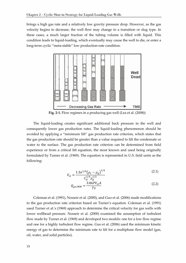
The flow regimes are largely classified as bubble flow, slug flow, slug-annular transition flow, or annular-mist flow, and are determined by the velocity of the gas and liquid phases and the relative amounts of gas and liquid at any given point in the flow stream. Gas well production from initial production to a liquid-loading condition is illustrated in Fig. 2-1. Initially, the well may show an annular-mist flow regime, which
Chapter 2 – Cyclic Shut-in Strategy for Liquid-Loading Gas Wells
19
brings a high gas rate and a relatively low gravity pressure drop. However, as the gas velocity begins to decrease, the well flow may change to a transition or slug type. In these cases, a much larger fraction of the tubing volume is filled with liquid. This condition leads to liquid-loading, which eventually may cause the well to die, or enter a long-term cyclic “meta-stable” low production-rate condition.
Fig. 2-1. Flow regimes in a producing gas well (Lea et al. (2008))
The liquid-loading creates significant additional back pressure in the well and
consequently lower gas production rates. The liquid-loading phenomenon should be avoided by applying a “minimum lift” gas production rate criterion, which states that the gas production rate should be greater than a value required to lift the condensate or water to the surface. The gas production rate criterion can be determined from field experience or from a critical lift equation, the most known and used being originally formulated by Turner et al. (1969). The equation is represented in U.S. field units as the following:
𝑉𝑠𝑙 =1.3𝜎1/4�𝜌𝐿 − 𝜌𝑔�
1/4
𝐶𝑑1/4𝜌𝑔
1/2 (2.1)
𝑄𝑔𝑠/𝑀𝑀 =3.06𝑃𝑃𝑉𝑠𝑙𝐴
𝑇𝑇𝑧 (2.2)
Coleman et al. (1991), Nosseir et al. (2000), and Guo et al. (2006) made modifications
to the gas production rate criterion based on Turner’s equation. Coleman et al. (1991) used Turner et al.'s (1969) approach to determine the critical velocity for gas wells with lower wellhead pressure. Nosseir et al. (2000) examined the assumption of turbulent flow made by Turner et al. (1969) and developed two models: one for a low flow regime and one for a highly turbulent flow regime. Guo et al. (2006) used the minimum kinetic energy of gas to determine the minimum rate to lift for a multiphase flow model (gas, oil, water, and solid particles).
Chapter 2 – Cyclic Shut-in Strategy for Liquid-Loading Gas Wells
20
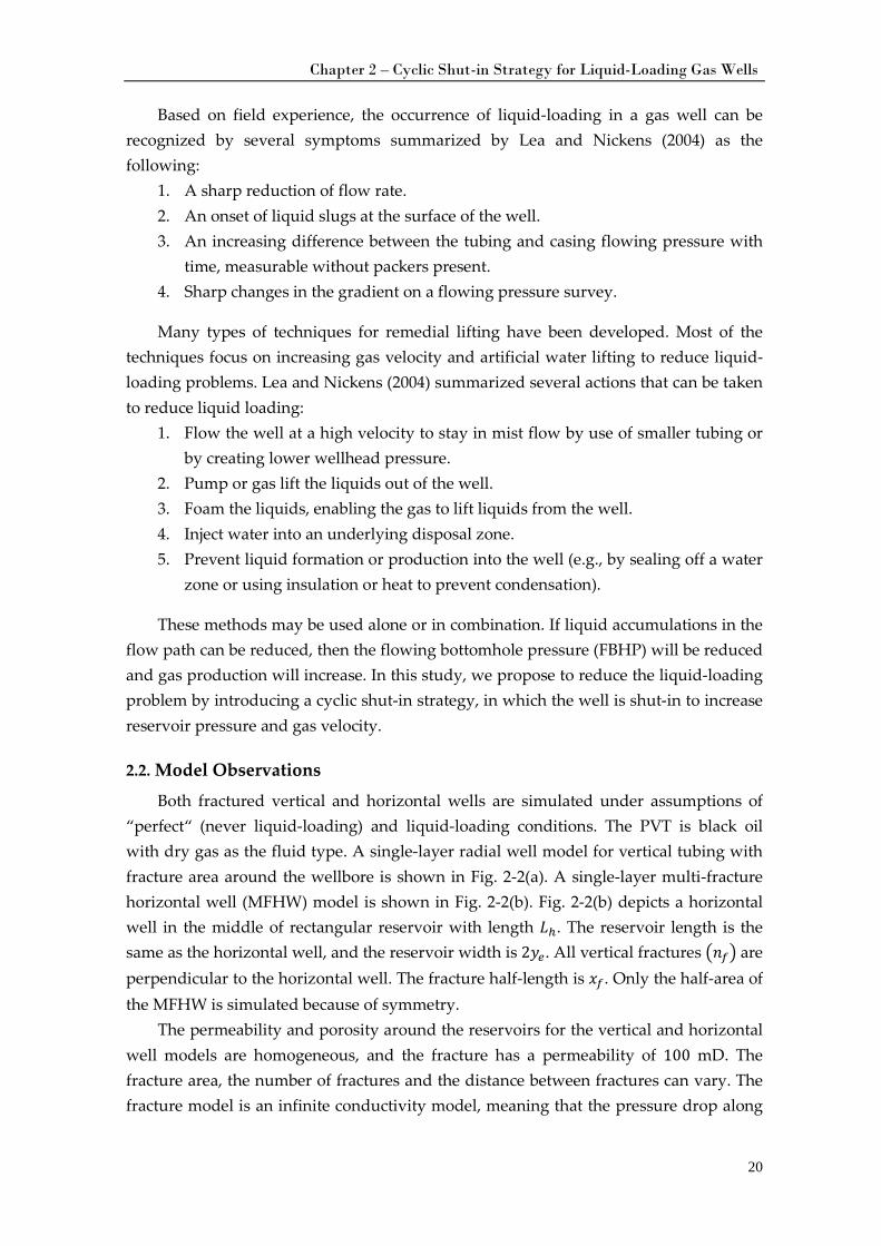
Based on field experience, the occurrence of liquid-loading in a gas well can be recognized by several symptoms summarized by Lea and Nickens (2004) as the following:
1. A sharp reduction of flow rate. 2. An onset of liquid slugs at the surface of the well. 3. An increasing difference between the tubing and casing flowing pressure with
time, measurable without packers present. 4. Sharp changes in the gradient on a flowing pressure survey.
Many types of techniques for remedial lifting have been developed. Most of the techniques focus on increasing gas velocity and artificial water lifting to reduce liquid-loading problems. Lea and Nickens (2004) summarized several actions that can be taken to reduce liquid loading:
1. Flow the well at a high velocity to stay in mist flow by use of smaller tubing or by creating lower wellhead pressure.
2. Pump or gas lift the liquids out of the well. 3. Foam the liquids, enabling the gas to lift liquids from the well. 4. Inject water into an underlying disposal zone. 5. Prevent liquid formation or production into the well (e.g., by sealing off a water
zone or using insulation or heat to prevent condensation).
These methods may be used alone or in combination. If liquid accumulations in the flow path can be reduced, then the flowing bottomhole pressure (FBHP) will be reduced and gas production will increase. In this study, we propose to reduce the liquid-loading problem by introducing a cyclic shut-in strategy, in which the well is shut-in to increase reservoir pressure and gas velocity.
2.2. Model Observations
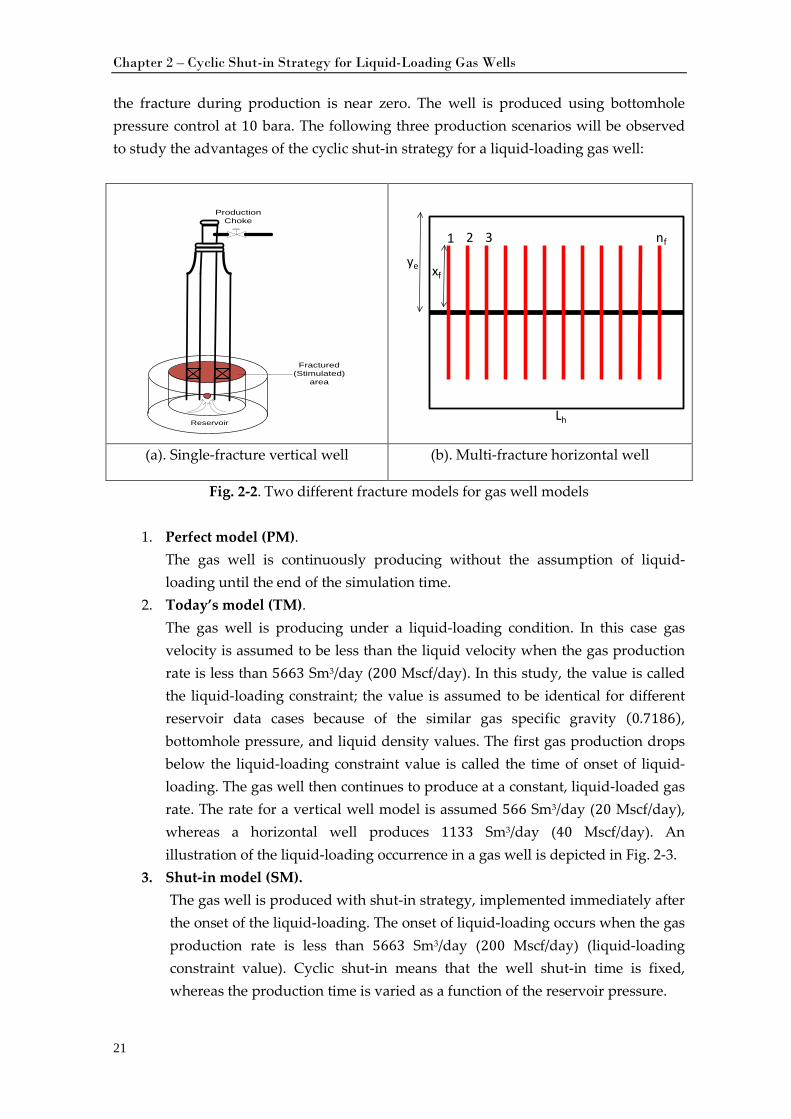
Both fractured vertical and horizontal wells are simulated under assumptions of “perfect“ (never liquid-loading) and liquid-loading conditions. The PVT is black oil with dry gas as the fluid type. A single-layer radial well model for vertical tubing with fracture area around the wellbore is shown in Fig. 2-2(a). A single-layer multi-fracture horizontal well (MFHW) model is shown in Fig. 2-2(b). Fig. 2-2(b) depicts a horizontal well in the middle of rectangular reservoir with length 𝐿𝐿ℎ. The reservoir length is the same as the horizontal well, and the reservoir width is 2𝑦𝑒. All vertical fractures �𝑛𝑓� are perpendicular to the horizontal well. The fracture half-length is 𝑥𝑓. Only the half-area of the MFHW is simulated because of symmetry.
The permeability and porosity around the reservoirs for the vertical and horizontal well models are homogeneous, and the fracture has a permeability of 100 mD. The fracture area, the number of fractures and the distance between fractures can vary. The fracture model is an infinite conductivity model, meaning that the pressure drop along
Chapter 2 – Cyclic Shut-in Strategy for Liquid-Loading Gas Wells
21
the fracture during production is near zero. The well is produced using bottomhole pressure control at 10 bara. The following three production scenarios will be observed to study the advantages of the cyclic shut-in strategy for a liquid-loading gas well:
(a). Single-fracture vertical well (b). Multi-fracture horizontal well
Fig. 2-2. Two different fracture models for gas well models
1. Perfect model (PM). The gas well is continuously producing without the assumption of liquid-loading until the end of the simulation time.
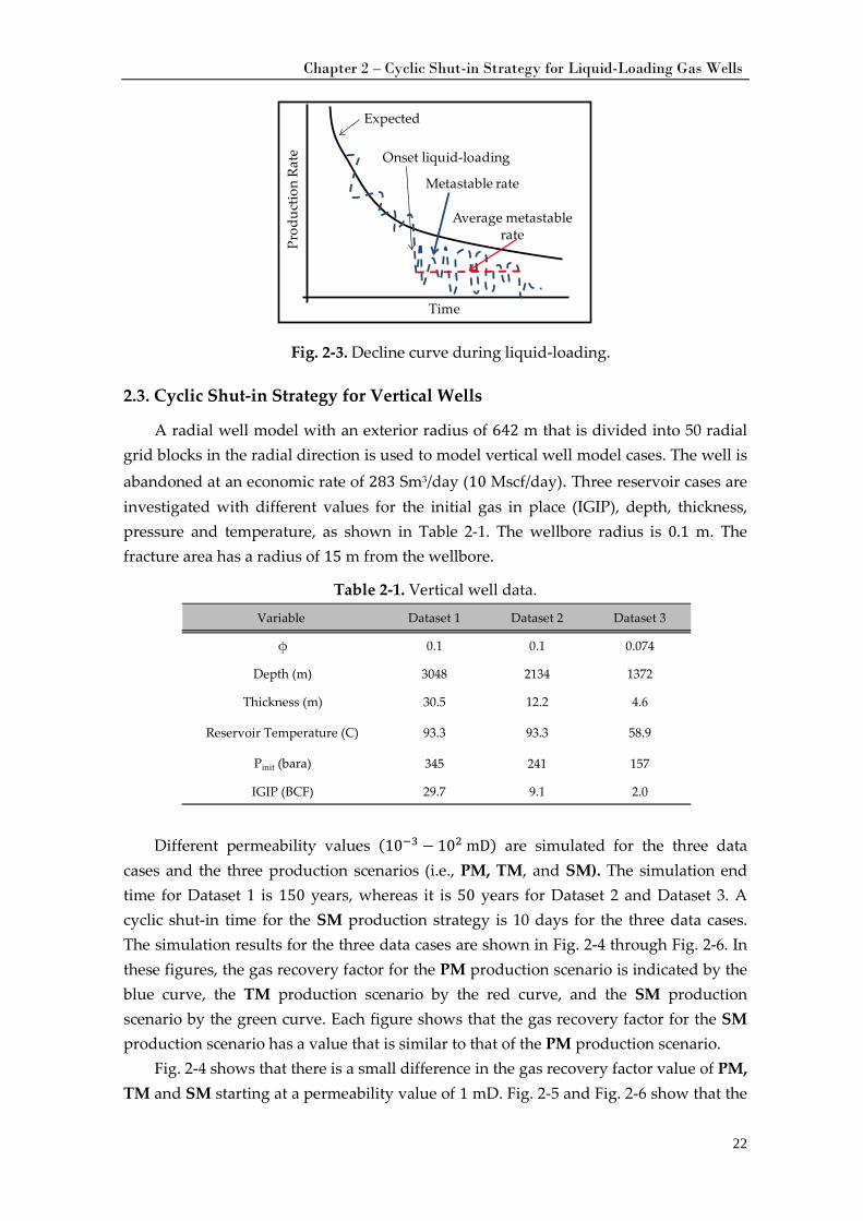
2. Today’s model (TM). The gas well is producing under a liquid-loading condition. In this case gas velocity is assumed to be less than the liquid velocity when the gas production rate is less than 5663 Sm3/day (200 Mscf/day). In this study, the value is called the liquid-loading constraint; the value is assumed to be identical for different reservoir data cases because of the similar gas specific gravity (0.7186), bottomhole pressure, and liquid density values. The first gas production drops below the liquid-loading constraint value is called the time of onset of liquid-loading. The gas well then continues to produce at a constant, liquid-loaded gas rate. The rate for a vertical well model is assumed 566 Sm3/day (20 Mscf/day), whereas a horizontal well produces 1133 Sm3/day (40 Mscf/day). An illustration of the liquid-loading occurrence in a gas well is depicted in Fig. 2-3.
3. Shut-in model (SM). The gas well is produced with shut-in strategy, implemented immediately after the onset of the liquid-loading. The onset of liquid-loading occurs when the gas production rate is less than 5663 Sm3/day (200 Mscf/day) (liquid-loading constraint value). Cyclic shut-in means that the well shut-in time is fixed, whereas the production time is varied as a function of the reservoir pressure.
ProductionChoke
Fractured (Stimulated)
area
Reservoir
ye
Lh
xf
1 2 3 nf
Chapter 2 – Cyclic Shut-in Strategy for Liquid-Loading Gas Wells
22
Fig. 2-3. Decline curve during liquid-loading.
2.3. Cyclic Shut-in Strategy for Vertical Wells
A radial well model with an exterior radius of 642 m that is divided into 50 radial grid blocks in the radial direction is used to model vertical well model cases. The well is abandoned at an economic rate of 283 Sm3/day (10 Mscf/day). Three reservoir cases are investigated with different values for the initial gas in place (IGIP), depth, thickness, pressure and temperature, as shown in Table 2-1. The wellbore radius is 0.1 m. The fracture area has a radius of 15 m from the wellbore.
Table 2-1. Vertical well data.
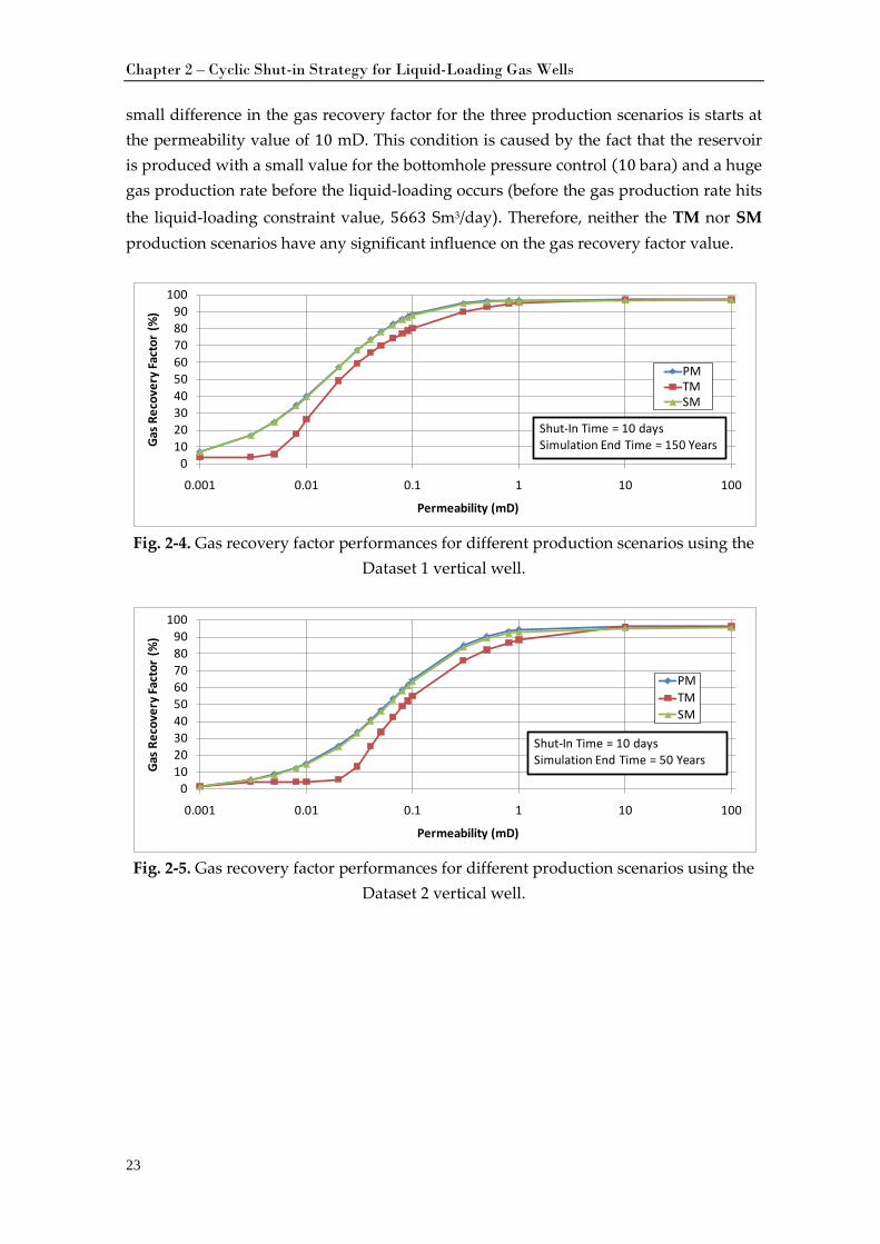
Different permeability values (10−3 − 102 mD) are simulated for the three data cases and the three production scenarios (i.e., PM, TM, and SM). The simulation end time for Dataset 1 is 150 years, whereas it is 50 years for Dataset 2 and Dataset 3. A cyclic shut-in time for the SM production strategy is 10 days for the three data cases. The simulation results for the three data cases are shown in Fig. 2-4 through Fig. 2-6. In these figures, the gas recovery factor for the PM production scenario is indicated by the blue curve, the TM production scenario by the red curve, and the SM production scenario by the green curve. Each figure shows that the gas recovery factor for the SM production scenario has a value that is similar to that of the PM production scenario.
Fig. 2-4 shows that there is a small difference in the gas recovery factor value of PM, TM and SM starting at a permeability value of 1 mD. Fig. 2-5 and Fig. 2-6 show that the
Prod
uctio
n Ra
teTime
Expected
Onset liquid-loading
Metastable rate
Average metastable rate
Variable Dataset 1 Dataset 2 Dataset 3
φ 0.1 0.1 0.074
Depth (m) 3048 2134 1372
Thickness (m) 30.5 12.2 4.6
Reservoir Temperature (C) 93.3 93.3 58.9
Pinit (bara) 345 241 157
IGIP (BCF) 29.7 9.1 2.0
Chapter 2 – Cyclic Shut-in Strategy for Liquid-Loading Gas Wells
23
small difference in the gas recovery factor for the three production scenarios is starts at the permeability value of 10 mD. This condition is caused by the fact that the reservoir is produced with a small value for the bottomhole pressure control (10 bara) and a huge gas production rate before the liquid-loading occurs (before the gas production rate hits the liquid-loading constraint value, 5663 Sm3/day). Therefore, neither the TM nor SM production scenarios have any significant influence on the gas recovery factor value.
Fig. 2-4. Gas recovery factor performances for different production scenarios using the
Dataset 1 vertical well.
Fig. 2-5. Gas recovery factor performances for different production scenarios using the
Dataset 2 vertical well.
0102030405060708090
100
0.001 0.01 0.1 1 10 100
Gas R
ecov
ery
Fact
or (%
)
Permeability (mD)
PMTMSM
Shut-In Time = 10 daysSimulation End Time = 150 Years
0102030405060708090
100
0.001 0.01 0.1 1 10 100
Gas R
ecov
ery
Fact
or (%
)
Permeability (mD)
PMTMSM
Shut-In Time = 10 daysSimulation End Time = 50 Years
Chapter 2 – Cyclic Shut-in Strategy for Liquid-Loading Gas Wells
24
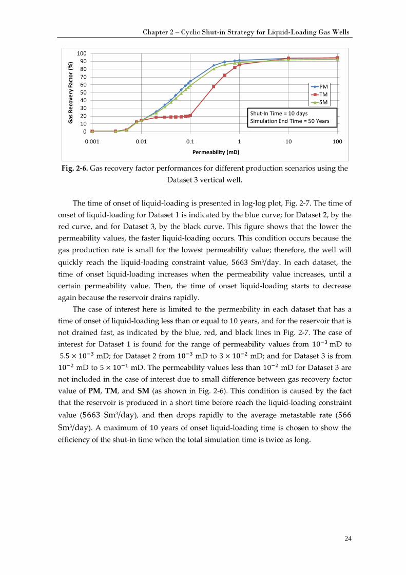
Fig. 2-6. Gas recovery factor performances for different production scenarios using the
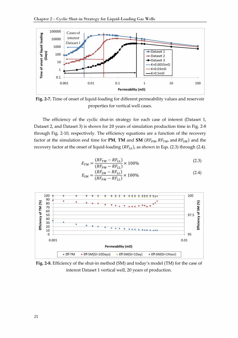
Dataset 3 vertical well. The time of onset of liquid-loading is presented in log-log plot, Fig. 2-7. The time of
onset of liquid-loading for Dataset 1 is indicated by the blue curve; for Dataset 2, by the red curve, and for Dataset 3, by the black curve. This figure shows that the lower the permeability values, the faster liquid-loading occurs. This condition occurs because the gas production rate is small for the lowest permeability value; therefore, the well will quickly reach the liquid-loading constraint value, 5663 Sm3/day. In each dataset, the time of onset liquid-loading increases when the permeability value increases, until a certain permeability value. Then, the time of onset liquid-loading starts to decrease again because the reservoir drains rapidly.
The case of interest here is limited to the permeability in each dataset that has a time of onset of liquid-loading less than or equal to 10 years, and for the reservoir that is not drained fast, as indicated by the blue, red, and black lines in Fig. 2-7. The case of interest for Dataset 1 is found for the range of permeability values from 10−3 mD to 5.5 × 10⁻³ mD; for Dataset 2 from 10−3 mD to 3 × 10⁻² mD; and for Dataset 3 is from 10−2 mD to 5 × 10⁻¹ mD. The permeability values less than 10−2 mD for Dataset 3 are not included in the case of interest due to small difference between gas recovery factor value of PM, TM, and SM (as shown in Fig. 2-6). This condition is caused by the fact that the reservoir is produced in a short time before reach the liquid-loading constraint value (5663 Sm3/day), and then drops rapidly to the average metastable rate (566 Sm3/day). A maximum of 10 years of onset liquid-loading time is chosen to show the efficiency of the shut-in time when the total simulation time is twice as long.
0102030405060708090
100
0.001 0.01 0.1 1 10 100
Gas R
ecov
ery
Fact
or (%
)
Permeability (mD)
PMTMSM
Shut-In Time = 10 daysSimulation End Time = 50 Years
Chapter 2 – Cyclic Shut-in Strategy for Liquid-Loading Gas Wells
25
Fig. 2-7. Time of onset of liquid-loading for different permeability values and reservoir
properties for vertical well cases.
The efficiency of the cyclic shut-in strategy for each case of interest (Dataset 1, Dataset 2, and Dataset 3) is shown for 20 years of simulation production time in Fig. 2-8 through Fig. 2-10, respectively. The efficiency equations are a function of the recovery factor at the simulation end time for PM, TM and SM (𝑅𝐹𝑃𝑀 ,𝑅𝐹𝑇𝑀, and 𝑅𝐹𝑆𝑀) and the recovery factor at the onset of liquid-loading (𝑅𝐹𝐿𝐿), as shown in Eqs. (2.3) through (2.4).
𝐸𝑇𝑀 =(𝑅𝐹𝑇𝑀 − 𝑅𝐹𝐿𝐿)(𝑅𝐹𝑃𝑀 − 𝑅𝐹𝐿𝐿) × 100% (2.3)
𝐸𝑆𝑀 =(𝑅𝐹𝑆𝑀 − 𝑅𝐹𝐿𝐿)(𝑅𝐹𝑃𝑀 − 𝑅𝐹𝐿𝐿) × 100% (2.4)
Fig. 2-8. Efficiency of the shut-in method (SM) and today’s model (TM) for the case of
interest Dataset 1 vertical well, 20 years of production.
0.1
1
10
100
1000
10000
100000
0.001 0.01 0.1 1 10 100
Tim
e of
ons
et o
f liq
uid
load
ing
(Day
s)
Permeability (mD)
Dataset 1Dataset 2Dataset 3K=0.0055mDK=0.03mDK=0.5mD
Cases of interest
Dataset 1
95
97.5
100
0102030405060708090
100
0.001 0.01
Effic
ienc
y of
SM
(%)
Effic
ienc
y of
TM
(%)
Permeability (mD)
Eff-TM Eff-SM(SI=10Days) Eff-SM(SI=1Day) Eff-SM(SI=1Hour)
Chapter 2 – Cyclic Shut-in Strategy for Liquid-Loading Gas Wells
26
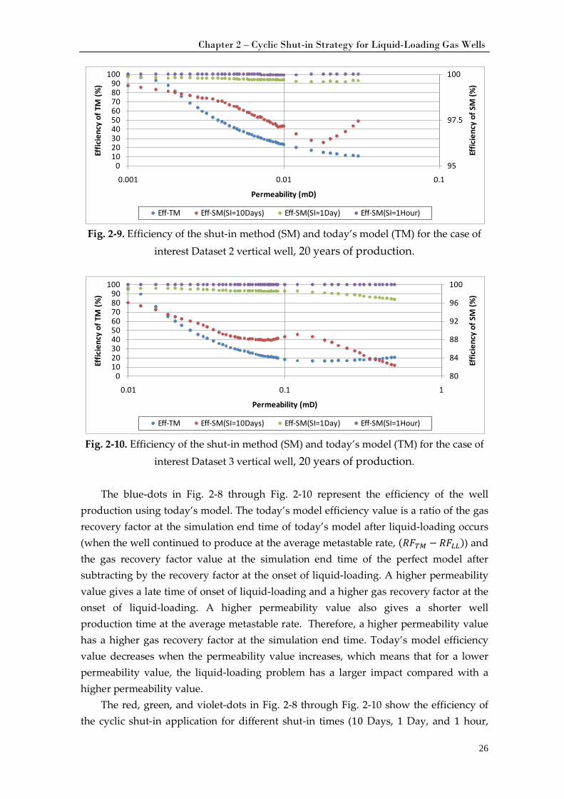
Fig. 2-9. Efficiency of the shut-in method (SM) and today’s model (TM) for the case of
interest Dataset 2 vertical well, 20 years of production.
Fig. 2-10. Efficiency of the shut-in method (SM) and today’s model (TM) for the case of
interest Dataset 3 vertical well, 20 years of production.
The blue-dots in Fig. 2-8 through Fig. 2-10 represent the efficiency of the well production using today’s model. The today’s model efficiency value is a ratio of the gas recovery factor at the simulation end time of today’s model after liquid-loading occurs (when the well continued to produce at the average metastable rate, (𝑅𝐹𝑇𝑀 − 𝑅𝐹𝐿𝐿)) and the gas recovery factor value at the simulation end time of the perfect model after subtracting by the recovery factor at the onset of liquid-loading. A higher permeability value gives a late time of onset of liquid-loading and a higher gas recovery factor at the onset of liquid-loading. A higher permeability value also gives a shorter well production time at the average metastable rate. Therefore, a higher permeability value has a higher gas recovery factor at the simulation end time. Today’s model efficiency value decreases when the permeability value increases, which means that for a lower permeability value, the liquid-loading problem has a larger impact compared with a higher permeability value.
The red, green, and violet-dots in Fig. 2-8 through Fig. 2-10 show the efficiency of the cyclic shut-in application for different shut-in times (10 Days, 1 Day, and 1 hour,
95
97.5
100
0102030405060708090
100
0.001 0.01 0.1
Effic
ienc
y of
SM
(%)
Effic
ienc
y of
TM
(%)
Permeability (mD)
Eff-TM Eff-SM(SI=10Days) Eff-SM(SI=1Day) Eff-SM(SI=1Hour)
80
84
88
92
96
100
0102030405060708090
100
0.01 0.1 1
Effic
ienc
y of
SM
(%)
Effic
ienc
y of
TM
(%)
Permeability (mD)
Eff-TM Eff-SM(SI=10Days) Eff-SM(SI=1Day) Eff-SM(SI=1Hour)
Chapter 2 – Cyclic Shut-in Strategy for Liquid-Loading Gas Wells
27
respectively). The shorter the cyclic shut-in time, the higher the gas recovery that can be achieved. This figure also shows that cyclic shut-in application is effective in reducing the gas production loss due to the occurrence of liquid-loading.
2.4. Cyclic Shut-in Strategy for Horizontal Wells
The scope of work for horizontal well model is broader than that for the vertical well model because an additional aspect is included, i.e., gridding sensitivity studies. A gridding study for a fractured horizontal well in a low permeability reservoir is reasonable to secure sufficient accuracy. Because of the homogeneity of the reservoir conditions, the study will be conducted for a single fracture horizontal well and a half reservoir area.
A heuristic method is used in this study by developing a systematic algorithm to find the “optimal” or “best” number of grid blocks in 𝑥 and 𝑦 directions. This algorithm is tested for a dry gas case, but it can also be used for liquids-rich gas producers.
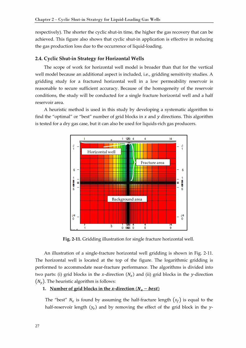
Fig. 2-11. Gridding illustration for single fracture horizontal well.
An illustration of a single-fracture horizontal well gridding is shown in Fig. 2-11. The horizontal well is located at the top of the figure. The logarithmic gridding is performed to accommodate near-fracture performance. The algorithms is divided into two parts: (i) grid blocks in the 𝑥-direction (𝑁𝑁𝑥) and (ii) grid blocks in the 𝑦-direction �𝑁𝑁𝑦�. The heuristic algorithm is follows:
1.
The “best” 𝑁𝑁𝑥 is found by assuming the half-fracture length �𝑥𝑓� is equal to the half-reservoir length (𝑦𝑒) and by removing the effect of the grid block in the 𝑦-
Number of grid blocks in the 𝒙-direction (𝑵𝒙 − 𝒃𝒆𝒔𝒕)
Horizontal well
Fracture area
Background area
Chapter 2 – Cyclic Shut-in Strategy for Liquid-Loading Gas Wells
28
direction. These assumptions are used to eliminate the gridding effect in the 𝑦-direction.
2.
Assumptions:
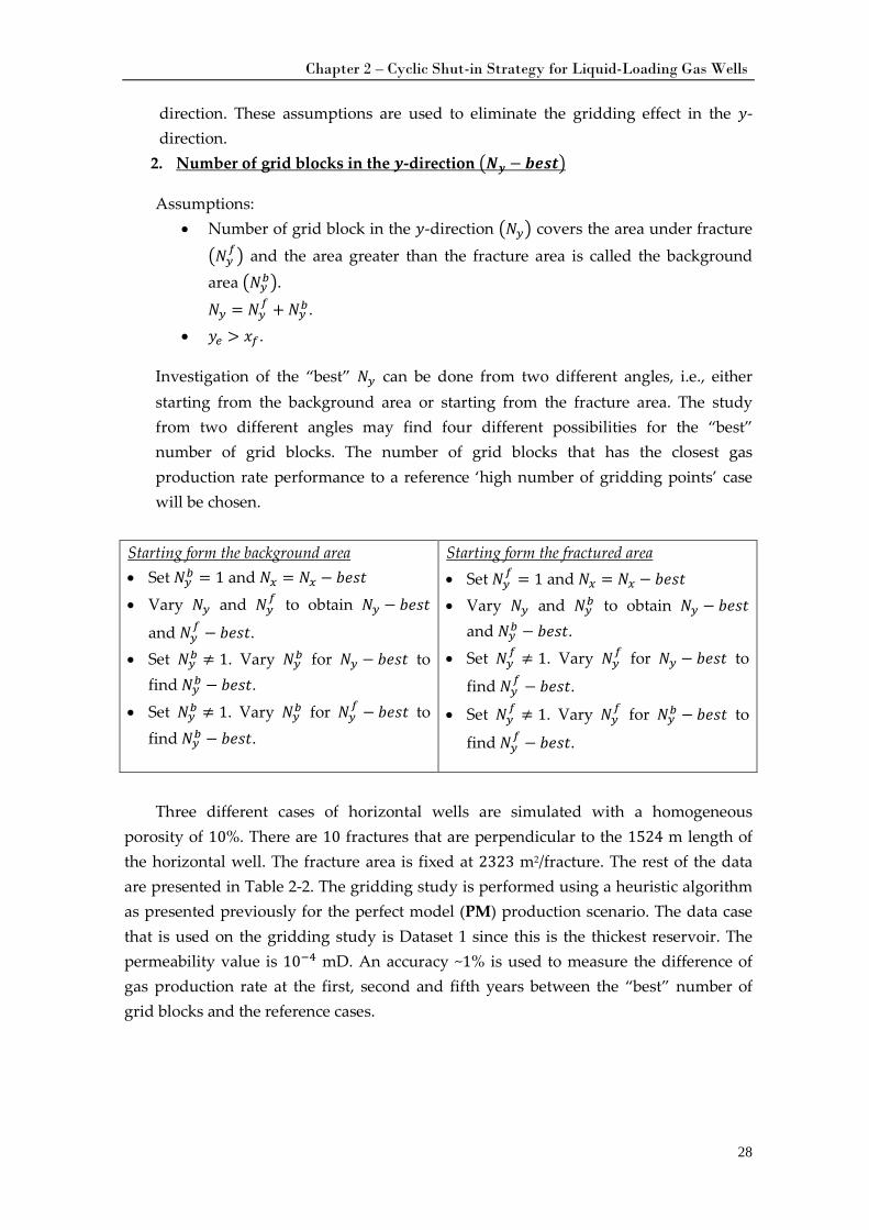
Number of grid blocks in the 𝒚-direction �𝑵𝒚 − 𝒃𝒆𝒔𝒕�
• Number of grid block in the 𝑦-direction �𝑁𝑁𝑦� covers the area under fracture
�𝑁𝑁𝑦𝑓� and the area greater than the fracture area is called the background
area �𝑁𝑁𝑦𝑏�.
𝑁𝑁𝑦 = 𝑁𝑁𝑦𝑓 + 𝑁𝑁𝑦𝑏.
• 𝑦𝑒 > 𝑥𝑓.
Investigation of the “best” 𝑁𝑁𝑦 can be done from two different angles, i.e., either starting from the background area or starting from the fracture area. The study from two different angles may find four different possibilities for the “best” number of grid blocks. The number of grid blocks that has the closest gas production rate performance to a reference ‘high number of gridding points’ case will be chosen.
• Set 𝑁𝑁𝑦𝑏 = 1 and 𝑁𝑁𝑥 = 𝑁𝑁𝑥 − 𝑏𝑠𝑠𝑠𝑠𝑡 Starting form the background area
• Vary 𝑁𝑁𝑦 and 𝑁𝑁𝑦𝑓 to obtain 𝑁𝑁𝑦 − 𝑏𝑠𝑠𝑠𝑠𝑡
and 𝑁𝑁𝑦𝑓 − 𝑏𝑠𝑠𝑠𝑠𝑡.
• Set 𝑁𝑁𝑦𝑏 ≠ 1. Vary 𝑁𝑁𝑦𝑏 for 𝑁𝑁𝑦 − 𝑏𝑠𝑠𝑠𝑠𝑡 to find 𝑁𝑁𝑦𝑏 − 𝑏𝑠𝑠𝑠𝑠𝑡.
• Set 𝑁𝑁𝑦𝑏 ≠ 1. Vary 𝑁𝑁𝑦𝑏 for 𝑁𝑁𝑦𝑓 − 𝑏𝑠𝑠𝑠𝑠𝑡 to
find 𝑁𝑁𝑦𝑏 − 𝑏𝑠𝑠𝑠𝑠𝑡.
• Set 𝑁𝑁𝑦𝑓 = 1 and 𝑁𝑁𝑥 = 𝑁𝑁𝑥 − 𝑏𝑠𝑠𝑠𝑠𝑡
Starting form the fractured area
• Vary 𝑁𝑁𝑦 and 𝑁𝑁𝑦𝑏 to obtain 𝑁𝑁𝑦 − 𝑏𝑠𝑠𝑠𝑠𝑡 and 𝑁𝑁𝑦𝑏 − 𝑏𝑠𝑠𝑠𝑠𝑡.
• Set 𝑁𝑁𝑦𝑓 ≠ 1. Vary 𝑁𝑁𝑦
𝑓 for 𝑁𝑁𝑦 − 𝑏𝑠𝑠𝑠𝑠𝑡 to
find 𝑁𝑁𝑦𝑓 − 𝑏𝑠𝑠𝑠𝑠𝑡.
• Set 𝑁𝑁𝑦𝑓 ≠ 1. Vary 𝑁𝑁𝑦
𝑓 for 𝑁𝑁𝑦𝑏 − 𝑏𝑠𝑠𝑠𝑠𝑡 to
find 𝑁𝑁𝑦𝑓 − 𝑏𝑠𝑠𝑠𝑠𝑡.
Three different cases of horizontal wells are simulated with a homogeneous
porosity of 10%. There are 10 fractures that are perpendicular to the 1524 m length of the horizontal well. The fracture area is fixed at 2323 m2/fracture. The rest of the data are presented in Table 2-2. The gridding study is performed using a heuristic algorithm as presented previously for the perfect model (PM) production scenario. The data case that is used on the gridding study is Dataset 1 since this is the thickest reservoir. The permeability value is 10−4 mD. An accuracy ~1% is used to measure the difference of gas production rate at the first, second and fifth years between the “best” number of grid blocks and the reference cases.
Chapter 2 – Cyclic Shut-in Strategy for Liquid-Loading Gas Wells
29
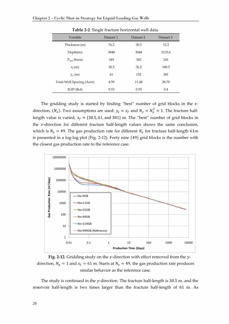
Table 2-2. Single fracture horizontal well data.
The gridding study is started by finding “best” number of grid blocks in the 𝑥-
direction, (𝑁𝑁𝑥). Two assumptions are used: 𝑦𝑒 = 𝑥𝑓 and 𝑁𝑁𝑦 = 𝑁𝑁𝑦𝑓 = 1. The fracture half-
length value is varied, 𝑥𝑓 = {30.5, 61, and 381} m. The “best” number of grid blocks in the 𝑥-direction for different fracture half-length values shows the same conclusion, which is 𝑁𝑁𝑥 = 49. The gas production rate for different 𝑁𝑁𝑥 for fracture half-length 61m is presented in a log-log plot (Fig. 2-12). Forty nine (49) grid blocks is the number with the closest gas production rate to the reference case.
Fig. 2-12. Gridding study on the 𝑥-direction with effect removed from the 𝑦-
direction, 𝑁𝑁𝑦 = 1 and 𝑥𝑓 = 61 m. Starts at 𝑁𝑁𝑥 = 49, the gas production rate produces similar behavior as the reference case.
The study is continued in the 𝑦-direction. The fracture half-length is 30.5 m, and the reservoir half-length is two times larger than the fracture half-length of 61 m. As
Variable Dataset 1 Dataset 2 Dataset 3
Thickness (m) 76.2 30.5 12.2
Depth(m) 3048 3048 2133.6
Pinit (bara) 345 345 241
xf (m) 30.5 76.2 190.5
ye (m) 61 152 381
Total Well Spacing (Acre) 4.59 11.48 28.70
IGIP (Bcf) 0.53 0.53 0.4
1
10
100
1000
10000
100000
1000000
10000000
0.01 0.1 1 10 100 1000 10000
Gas P
rodu
ctio
n Ra
te (m
3 /da
y)
Production Time (Days)
Nx=9GB
Nx=11GB
Nx=25GB
Nx=49GB
Nx=159GB
Nx=999GB (Reference)
Chapter 2 – Cyclic Shut-in Strategy for Liquid-Loading Gas Wells
30
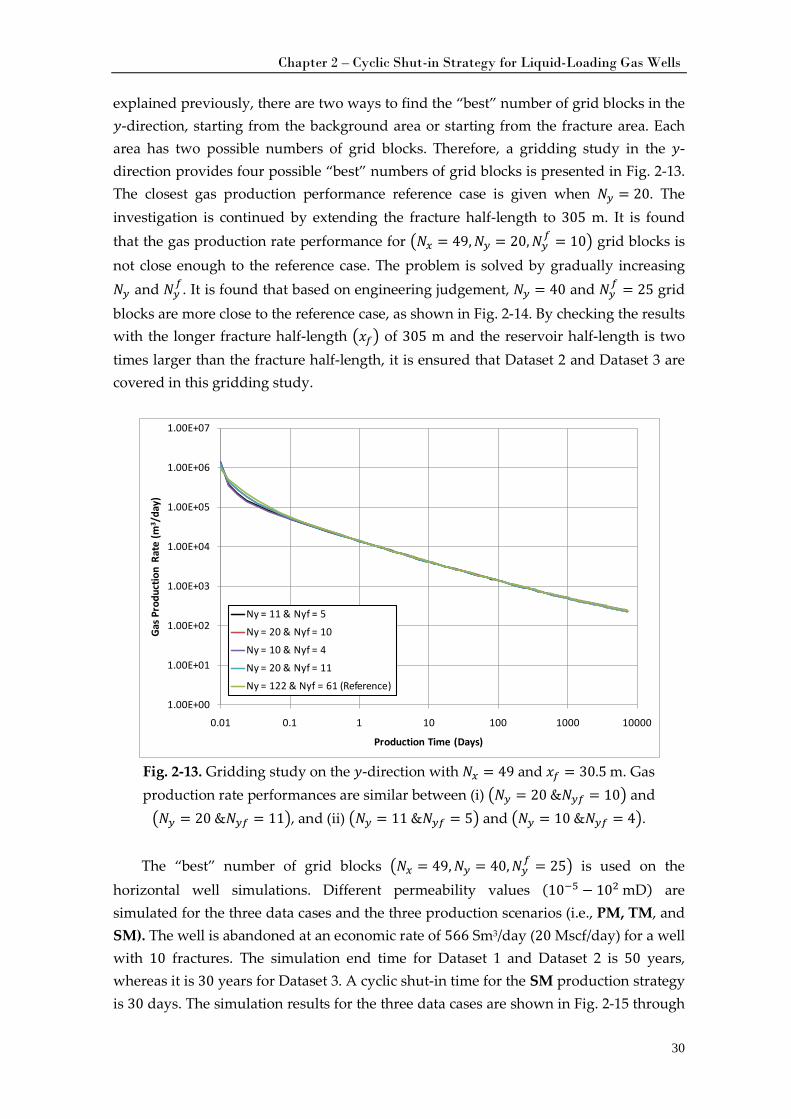
explained previously, there are two ways to find the “best” number of grid blocks in the 𝑦-direction, starting from the background area or starting from the fracture area. Each area has two possible numbers of grid blocks. Therefore, a gridding study in the 𝑦-direction provides four possible “best” numbers of grid blocks is presented in Fig. 2-13. The closest gas production performance reference case is given when 𝑁𝑁𝑦 = 20. The investigation is continued by extending the fracture half-length to 305 m. It is found that the gas production rate performance for �𝑁𝑁𝑥 = 49,𝑁𝑁𝑦 = 20,𝑁𝑁𝑦
𝑓 = 10� grid blocks is not close enough to the reference case. The problem is solved by gradually increasing 𝑁𝑁𝑦 and 𝑁𝑁𝑦
𝑓. It is found that based on engineering judgement, 𝑁𝑁𝑦 = 40 and 𝑁𝑁𝑦𝑓 = 25 grid
blocks are more close to the reference case, as shown in Fig. 2-14. By checking the results with the longer fracture half-length �𝑥𝑓� of 305 m and the reservoir half-length is two times larger than the fracture half-length, it is ensured that Dataset 2 and Dataset 3 are covered in this gridding study.
Fig. 2-13. Gridding study on the 𝑦-direction with 𝑁𝑁𝑥 = 49 and 𝑥𝑓 = 30.5 m. Gas production rate performances are similar between (i) �𝑁𝑁𝑦 = 20 &𝑁𝑁𝑦𝑓 = 10� and �𝑁𝑁𝑦 = 20 &𝑁𝑁𝑦𝑓 = 11�, and (ii) �𝑁𝑁𝑦 = 11 &𝑁𝑁𝑦𝑓 = 5� and �𝑁𝑁𝑦 = 10 &𝑁𝑁𝑦𝑓 = 4�.
The “best” number of grid blocks �𝑁𝑁𝑥 = 49,𝑁𝑁𝑦 = 40,𝑁𝑁𝑦
𝑓 = 25� is used on the horizontal well simulations. Different permeability values (10−5 − 102 mD) are simulated for the three data cases and the three production scenarios (i.e., PM, TM, and SM). The well is abandoned at an economic rate of 566 Sm3/day (20 Mscf/day) for a well with 10 fractures. The simulation end time for Dataset 1 and Dataset 2 is 50 years, whereas it is 30 years for Dataset 3. A cyclic shut-in time for the SM production strategy is 30 days. The simulation results for the three data cases are shown in Fig. 2-15 through
1.00E+00
1.00E+01
1.00E+02
1.00E+03
1.00E+04
1.00E+05
1.00E+06
1.00E+07
0.01 0.1 1 10 100 1000 10000
Gas P
rodu
ctio
n Ra
te (m
3 /da
y)
Production Time (Days)
Ny = 11 & Nyf = 5
Ny = 20 & Nyf = 10
Ny = 10 & Nyf = 4
Ny = 20 & Nyf = 11
Ny = 122 & Nyf = 61 (Reference)
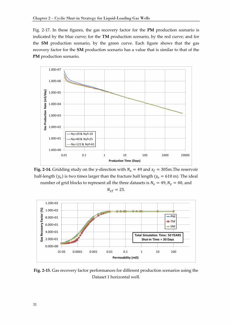
Chapter 2 – Cyclic Shut-in Strategy for Liquid-Loading Gas Wells
31
Fig. 2-17. In these figures, the gas recovery factor for the PM production scenario is indicated by the blue curve; for the TM production scenario, by the red curve; and for the SM production scenario, by the green curve. Each figure shows that the gas recovery factor for the SM production scenario has a value that is similar to that of the PM production scenario.
Fig. 2-14. Gridding study on the 𝑦-direction with 𝑁𝑁𝑥 = 49 and 𝑥𝑓 = 305m.The reservoir half-length (𝑦𝑒) is two times larger than the fracture half length (𝑦𝑒 = 610 m). The ideal
number of grid blocks to represent all the three datasets is 𝑁𝑁𝑥 = 49,𝑁𝑁𝑦 = 40, and 𝑁𝑁𝑦𝑓 = 25.
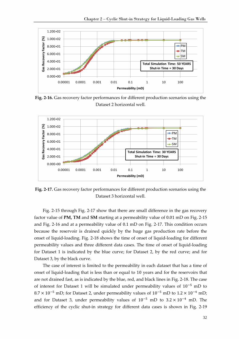
Fig. 2-15. Gas recovery factor performances for different production scenarios using the Dataset 1 horizontal well.
1.00E+00
1.00E+01
1.00E+02
1.00E+03
1.00E+04
1.00E+05
1.00E+06
1.00E+07
0.01 0.1 1 10 100 1000 10000
Gas P
rodu
ctio
n Ra
te (m
3/da
y)
Production Time (Days)
Ny=20 & Nyf=10
Ny=40 & Nyf=25
Ny=122 & Nyf=61
0.00E+00
2.00E+01
4.00E+01
6.00E+01
8.00E+01
1.00E+02
1.20E+02
1E-05 0.0001 0.001 0.01 0.1 1 10 100
Gas R
ecov
ery
Fact
or (%
)
Permeability (mD)
PMTMSM
Total Simulation Time: 50 YEARSShut-in Time = 30 Days
Chapter 2 – Cyclic Shut-in Strategy for Liquid-Loading Gas Wells
32
Fig. 2-16. Gas recovery factor performances for different production scenarios using the
Dataset 2 horizontal well.
Fig. 2-17. Gas recovery factor performances for different production scenarios using the Dataset 3 horizontal well.
Fig. 2-15 through Fig. 2-17 show that there are small difference in the gas recovery
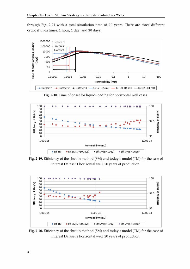
factor value of PM, TM and SM starting at a permeability value of 0.01 mD on Fig. 2-15 and Fig. 2-16 and at a permeability value of 0.1 mD on Fig. 2-17. This condition occurs because the reservoir is drained quickly by the huge gas production rate before the onset of liquid-loading. Fig. 2-18 shows the time of onset of liquid-loading for different permeability values and three different data cases. The time of onset of liquid-loading for Dataset 1 is indicated by the blue curve; for Dataset 2, by the red curve; and for Dataset 3, by the black curve.
The case of interest is limited to the permeability in each dataset that has a time of onset of liquid-loading that is less than or equal to 10 years and for the reservoirs that are not drained fast, as is indicated by the blue, red, and black lines in Fig. 2-18. The case of interest for Dataset 1 will be simulated under permeability values of 10−5 mD to 8.7 × 10⁻⁵ mD; for Dataset 2, under permeability values of 10−5 mD to 1.2 × 10⁻⁴ mD; and for Dataset 3, under permeability values of 10−5 mD to 3.2 × 10⁻⁴ mD. The efficiency of the cyclic shut-in strategy for different data cases is shown in Fig. 2-19
0.00E+00
2.00E+01
4.00E+01
6.00E+01
8.00E+01
1.00E+02
1.20E+02
0.00001 0.0001 0.001 0.01 0.1 1 10 100
Gas R
ecov
ery
Fact
or (%
)
Permeability (mD)
PMTMSM
Total Simulation Time: 50 YEARSShut-in Time = 30 Days
0.00E+00
2.00E+01
4.00E+01
6.00E+01
8.00E+01
1.00E+02
1.20E+02
0.00001 0.0001 0.001 0.01 0.1 1 10 100
Gas R
ecov
ery
Fact
or (%
)
Permeability (mD)
PMTMSM
Total Simulation Time: 30 YEARSShut-in Time = 30 Days
Chapter 2 – Cyclic Shut-in Strategy for Liquid-Loading Gas Wells
33
through Fig. 2-21 with a total simulation time of 20 years. There are three different cyclic shut-in times: 1 hour, 1 day, and 30 days.
Fig. 2-18. Time of onset for liquid-loading for horizontal well cases.
Fig. 2-19. Efficiency of the shut-in method (SM) and today’s model (TM) for the case of
interest Dataset 1 horizontal well, 20 years of production.
Fig. 2-20. Efficiency of the shut-in method (SM) and today’s model (TM) for the case of
interest Dataset 2 horizontal well, 20 years of production.
1
10
100
1000
10000
100000
1000000
0.00001 0.0001 0.001 0.01 0.1 1 10 100Tim
e of
ons
et o
f liq
uid-
load
ing
(Day
s)
Permeability (mD)
Dataset 1 Dataset 2 Dataset 3 K=8.7E-05 mD K=1.2E-04 mD K=3.2E-04 mD
Cases of interest
Dataset 1
95
97.5
100
0102030405060708090
100
1.00E-05 1.00E-04
Effic
ienc
y of
SM
(%)
Effic
ienc
y of
TM
(%)
Permeability (mD)
Eff-TM Eff-SM(SI=30Days) Eff-SM(SI=1Day) Eff-SM(SI=1Hour)
95
97.5
100
0102030405060708090
100
1.00E-05 1.00E-04 1.00E-03
Effic
ienc
y of
SM
(%)
Effic
ienc
y of
TM
(%)
Permeability (mD)
Eff-TM Eff-SM(SI=30Days) Eff-SM(SI=1Day) Eff-SM(SI=1Hour)
Chapter 2 – Cyclic Shut-in Strategy for Liquid-Loading Gas Wells
34
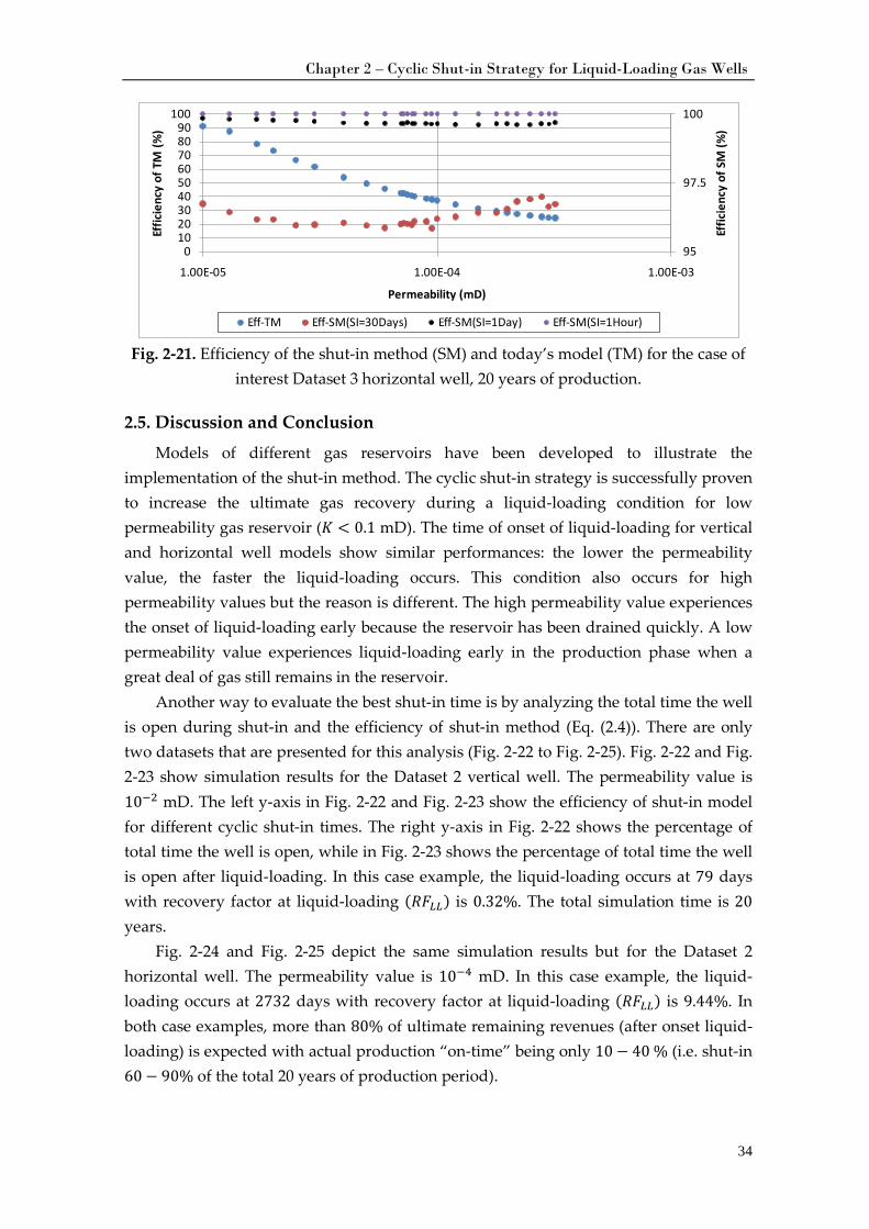
Fig. 2-21. Efficiency of the shut-in method (SM) and today’s model (TM) for the case of
interest Dataset 3 horizontal well, 20 years of production.
2.5. Discussion and Conclusion
Models of different gas reservoirs have been developed to illustrate the implementation of the shut-in method. The cyclic shut-in strategy is successfully proven to increase the ultimate gas recovery during a liquid-loading condition for low permeability gas reservoir (𝐾 < 0.1 mD). The time of onset of liquid-loading for vertical and horizontal well models show similar performances: the lower the permeability value, the faster the liquid-loading occurs. This condition also occurs for high permeability values but the reason is different. The high permeability value experiences the onset of liquid-loading early because the reservoir has been drained quickly. A low permeability value experiences liquid-loading early in the production phase when a great deal of gas still remains in the reservoir.
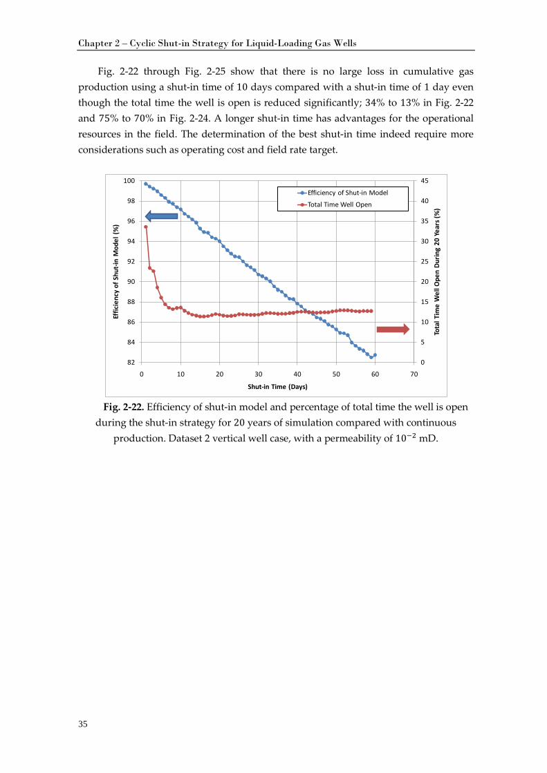
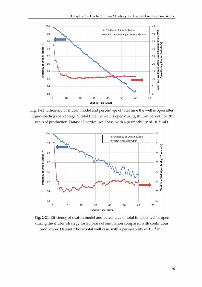
Another way to evaluate the best shut-in time is by analyzing the total time the well is open during shut-in and the efficiency of shut-in method (Eq. (2.4)). There are only two datasets that are presented for this analysis (Fig. 2-22 to Fig. 2-25). Fig. 2-22 and Fig. 2-23 show simulation results for the Dataset 2 vertical well. The permeability value is 10−2 mD. The left y-axis in Fig. 2-22 and Fig. 2-23 show the efficiency of shut-in model for different cyclic shut-in times. The right y-axis in Fig. 2-22 shows the percentage of total time the well is open, while in Fig. 2-23 shows the percentage of total time the well is open after liquid-loading. In this case example, the liquid-loading occurs at 79 days with recovery factor at liquid-loading (𝑅𝐹𝐿𝐿) is 0.32%. The total simulation time is 20 years.
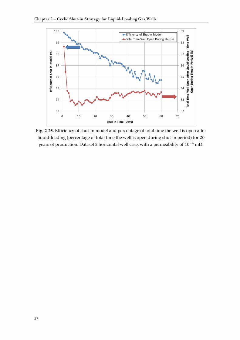
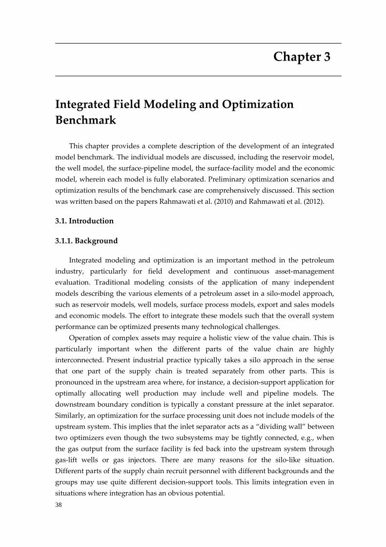
Fig. 2-24 and Fig. 2-25 depict the same simulation results but for the Dataset 2 horizontal well. The permeability value is 10−4 mD. In this case example, the liquid-loading occurs at 2732 days with recovery factor at liquid-loading (𝑅𝐹𝐿𝐿) is 9.44%. In both case examples, more than 80% of ultimate remaining revenues (after onset liquid-loading) is expected with actual production “on-time” being only 10 − 40 % (i.e. shut-in 60 − 90% of the total 20 years of production period).
95
97.5
100
0102030405060708090
100
1.00E-05 1.00E-04 1.00E-03
Effic
ienc
y of
SM
(%)
Effic
ienc
y of
TM
(%)
Permeability (mD)
Eff-TM Eff-SM(SI=30Days) Eff-SM(SI=1Day) Eff-SM(SI=1Hour)
Chapter 2 – Cyclic Shut-in Strategy for Liquid-Loading Gas Wells
35
Fig. 2-22 through Fig. 2-25 show that there is no large loss in cumulative gas production using a shut-in time of 10 days compared with a shut-in time of 1 day even though the total time the well is open is reduced significantly; 34% to 13% in Fig. 2-22 and 75% to 70% in Fig. 2-24. A longer shut-in time has advantages for the operational resources in the field. The determination of the best shut-in time indeed require more considerations such as operating cost and field rate target.
Fig. 2-22. Efficiency of shut-in model and percentage of total time the well is open
during the shut-in strategy for 20 years of simulation compared with continuous production. Dataset 2 vertical well case, with a permeability of 10−2 mD.
0
5
10
15
20
25
30
35
40
45
82
84
86
88
90
92
94
96
98
100
0 10 20 30 40 50 60 70
Tota
l Tim
e W
ell O
pen
Durin
g 20
Yea
rs (%
)
Effic
ienc
y of
Shu
t-in
Mod
el (
%)
Shut-in Time (Days)
Efficiency of Shut-in Model
Total Time Well Open
Chapter 2 – Cyclic Shut-in Strategy for Liquid-Loading Gas Wells
36
Fig. 2-23. Efficiency of shut-in model and percentage of total time the well is open after liquid-loading (percentage of total time the well is open during shut-in period) for 20
years of production. Dataset 2 vertical well case, with a permeability of 10−2 mD.
Fig. 2-24. Efficiency of shut-in model and percentage of total time the well is open during the shut-in strategy for 20 years of simulation compared with continuous
production. Dataset 2 horizontal well case, with a permeability of 10−4 mD.
0
5
10
15
20
25
30
35
40
45
82
84
86
88
90
92
94
96
98
100
0 10 20 30 40 50 60 70
Tota
l Tim
e W
ell O
pen
Afte
r Liq
uid -
Load
ing
(Tim
e W
ell
Ope
n Du
ring
Shut
-in P
erio
d) (%
)
Effic
ienc
y of
Shu
t-in
Mod
el (
%)
Shut-in Time (Days)
Efficiency of Shut-in Model
Total Time Well Open During Shut-in
69
70
71
72
73
74
75
76
93
94
95
96
97
98
99
100
0 10 20 30 40 50 60 70
Tota
l tim
e W
ell O
pen
Durin
g 20
Yea
rs (%
)
Effic
ienc
y of
Shu
t-in
Mod
el (
%)
Shut-in Time (Days)
Efficiency of Shut-in ModelTotal Time Well Open
Chapter 2 – Cyclic Shut-in Strategy for Liquid-Loading Gas Wells
37
Fig. 2-25. Efficiency of shut-in model and percentage of total time the well is open after liquid-loading (percentage of total time the well is open during shut-in period) for 20 years of production. Dataset 2 horizontal well case, with a permeability of 10−4 mD.
32
33
34
35
36
37
38
39
93
94
95
96
97
98
99
100
0 10 20 30 40 50 60 70
Tota
l Tim
e W
ell O
pen
Afte
r Liq
uid -
Load
ing
(Tim
e W
ell
Ope
n Du
ring
Shut
-in P
erio
d) (%
)
Effic
ienc
y of
Shu
t-in
Mod
el (
%)
Shut-in Time (Days)
Efficiency of Shut-in ModelTotal Time Well Open During Shut-in
38
Chapter 3
Integrated Field Modeling and Optimization Benchmark
This chapter provides a complete description of the development of an integrated model benchmark. The individual models are discussed, including the reservoir model, the well model, the surface-pipeline model, the surface-facility model and the economic model, wherein each model is fully elaborated. Preliminary optimization scenarios and optimization results of the benchmark case are comprehensively discussed. This section was written based on the papers Rahmawati et al. (2010) and Rahmawati et al. (2012).
3.1. Introduction
3.1.1. Background
Integrated modeling and optimization is an important method in the petroleum industry, particularly for field development and continuous asset-management evaluation. Traditional modeling consists of the application of many independent models describing the various elements of a petroleum asset in a silo-model approach, such as reservoir models, well models, surface process models, export and sales models and economic models. The effort to integrate these models such that the overall system performance can be optimized presents many technological challenges.
Operation of complex assets may require a holistic view of the value chain. This is particularly important when the different parts of the value chain are highly interconnected. Present industrial practice typically takes a silo approach in the sense that one part of the supply chain is treated separately from other parts. This is pronounced in the upstream area where, for instance, a decision-support application for optimally allocating well production may include well and pipeline models. The downstream boundary condition is typically a constant pressure at the inlet separator. Similarly, an optimization for the surface processing unit does not include models of the upstream system. This implies that the inlet separator acts as a “dividing wall” between two optimizers even though the two subsystems may be tightly connected, e.g., when the gas output from the surface facility is fed back into the upstream system through gas-lift wells or gas injectors. There are many reasons for the silo-like situation. Different parts of the supply chain recruit personnel with different backgrounds and the groups may use quite different decision-support tools. This limits integration even in situations where integration has an obvious potential.
Chapter 3 – Integrated Field Modeling and Optimization Benchmark
39
Many researchers have conducted studies on various integration topics. Cullick et al. (2003), Bailey et al. (2005), Ogunyomi et al. (2011), and Litvak et al. (2011) discussed complex petroleum field projects applying uncertainty analysis, but the complexity of surface process facility was not considered. Nazarian (2002) integrated ECLIPSE® and HYSYS® simulators to calculate integrated field operation in a deepwater oil field. These simulators were coupled with an Automation and Parallel Virtual Machine approach and with application of a genetic algorithm for the optimization. Hepguler et al. (1997) and Hepguler et al. (1997a) discussed an integrated application for reservoir-production strategies and field-development management. In this case, the ECLIPSE reservoir simulator was coupled with the surface and production-network simulator and the optimizer (Netopt). Run time can be a challenge in integrated applications, especially when high-fidelity models are closely linked.
Barroux et al. (2000) presented an integrated model consists of a reservoir simulator and a steady-state network simulator. The paper is intended to contribute to a better communication between reservoir, production, surface and process engineers. Using the same interface, Trick (1998) applied a somewhat different procedure than Hepguler et al. (1997). In this case, an ECLIPSE black-oil reservoir simulator was coupled to a surface gas deliverability forecasting model, FORGAS. The use of integrated optimization in the day-to-day operations setting of the LNG value chain was studied by Foss and Halvorsen (2009). To reduce computation time, they chose simple models for all system components. A sizable reduction was obtained by integrating all the models into one decision-support application as opposed to dividing them into two applications; one for the upstream part and the other for the LNG plant. Tomasgard et al. (2007) presented a natural gas value-chain model and integration applying an upstream perspective and a stochastic portfolio optimization.
Galic et al. (2009) applied integrated asset modeling (IAM) in planning CO2 injection into depleted reservoirs. By implementing IAM, the flow-assurance problem during CO2 injection could be recognized and a plateau-injection rate maintained. The toolkit used here included REVEAL for reservoir simulation, PROSPER for wells and network simulation, GAP for the surface network, the RESOLVE simulator for maintaining dynamic simulation from the reservoir to the surface processing and PVTP for PVT simulation. Kosmala et al. (2003) integrated reservoir and network models for two fields. One field undergoes a Water Alternating Gas (WAG) process and the other field undergoes gas lift. Integrated model implementation provided advantageous for improving oil production by optimizing injection rate allocation for these two scenarios. Couët et al. (2010) optimized gas lift allocation by implementing an adaptive proxy on the integrated asset modeling approach to reduce computational time.
Applications of integrated models have been developed at several companies such as BG, Madray et al. (2008). An integrated model has been implemented at Miskar Field, Tunisia. The objectives were to optimize the production, monitor the gas blend sent to the beach and capture the well rate. Another leading company in the application of
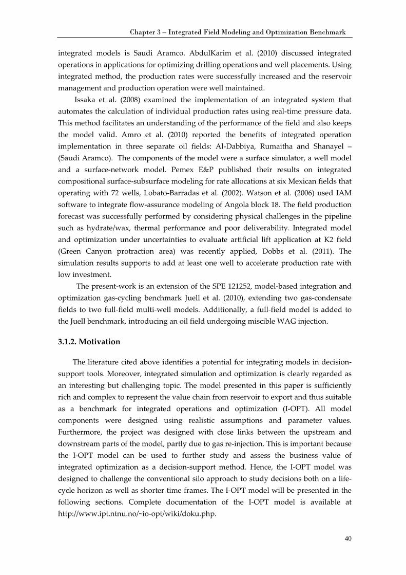
Chapter 3 – Integrated Field Modeling and Optimization Benchmark
40
integrated models is Saudi Aramco. AbdulKarim et al. (2010) discussed integrated operations in applications for optimizing drilling operations and well placements. Using integrated method, the production rates were successfully increased and the reservoir management and production operation were well maintained.
Issaka et al. (2008) examined the implementation of an integrated system that automates the calculation of individual production rates using real-time pressure data. This method facilitates an understanding of the performance of the field and also keeps the model valid. Amro et al. (2010) reported the benefits of integrated operation implementation in three separate oil fields: Al-Dabbiya, Rumaitha and Shanayel – (Saudi Aramco). The components of the model were a surface simulator, a well model and a surface-network model. Pemex E&P published their results on integrated compositional surface-subsurface modeling for rate allocations at six Mexican fields that operating with 72 wells, Lobato-Barradas et al. (2002). Watson et al. (2006) used IAM software to integrate flow-assurance modeling of Angola block 18. The field production forecast was successfully performed by considering physical challenges in the pipeline such as hydrate/wax, thermal performance and poor deliverability. Integrated model and optimization under uncertainties to evaluate artificial lift application at K2 field (Green Canyon protraction area) was recently applied, Dobbs et al. (2011). The simulation results supports to add at least one well to accelerate production rate with low investment.
The present-work is an extension of the SPE 121252, model-based integration and optimization gas-cycling benchmark Juell et al. (2010), extending two gas-condensate fields to two full-field multi-well models. Additionally, a full-field model is added to the Juell benchmark, introducing an oil field undergoing miscible WAG injection.
3.1.2. Motivation
The literature cited above identifies a potential for integrating models in decision-support tools. Moreover, integrated simulation and optimization is clearly regarded as an interesting but challenging topic. The model presented in this paper is sufficiently rich and complex to represent the value chain from reservoir to export and thus suitable as a benchmark for integrated operations and optimization (I-OPT). All model components were designed using realistic assumptions and parameter values. Furthermore, the project was designed with close links between the upstream and downstream parts of the model, partly due to gas re-injection. This is important because the I-OPT model can be used to further study and assess the business value of integrated optimization as a decision-support method. Hence, the I-OPT model was designed to challenge the conventional silo approach to study decisions both on a life-cycle horizon as well as shorter time frames. The I-OPT model will be presented in the following sections. Complete documentation of the I-OPT model is available at http://www.ipt.ntnu.no/~io-opt/wiki/doku.php.
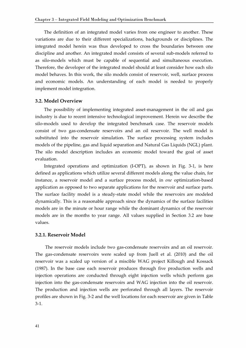
Chapter 3 – Integrated Field Modeling and Optimization Benchmark
41
The definition of an integrated model varies from one engineer to another. These variations are due to their different specializations, backgrounds or disciplines. The integrated model herein was thus developed to cross the boundaries between one discipline and another. An integrated model consists of several sub-models referred to as silo-models which must be capable of sequential and simultaneous execution. Therefore, the developer of the integrated model should at least consider how each silo model behaves. In this work, the silo models consist of reservoir, well, surface process and economic models. An understanding of each model is needed to properly implement model integration.
3.2. Model Overview
The possibility of implementing integrated asset-management in the oil and gas industry is due to recent intensive technological improvement. Herein we describe the silo-models used to develop the integrated benchmark case. The reservoir models consist of two gas-condensate reservoirs and an oil reservoir. The well model is substituted into the reservoir simulation. The surface processing system includes models of the pipeline, gas and liquid separation and Natural Gas Liquids (NGL) plant. The silo model description includes an economic model toward the goal of asset evaluation.
Integrated operations and optimization (I-OPT), as shown in Fig. 3-1, is here defined as applications which utilize several different models along the value chain, for instance, a reservoir model and a surface process model, in one optimization-based application as opposed to two separate applications for the reservoir and surface parts. The surface facility model is a steady-state model while the reservoirs are modeled dynamically. This is a reasonable approach since the dynamics of the surface facilities models are in the minute or hour range while the dominant dynamics of the reservoir models are in the months to year range. All values supplied in Section 3.2 are base values.
3.2.1. Reservoir Model
The reservoir models include two gas-condensate reservoirs and an oil reservoir. The gas-condensate reservoirs were scaled up from Juell et al. (2010) and the oil reservoir was a scaled up version of a miscible WAG project Killough and Kossack (1987). In the base case each reservoir produces through five production wells and injection operations are conducted through eight injection wells which perform gas injection into the gas-condensate reservoirs and WAG injection into the oil reservoir. The production and injection wells are perforated through all layers. The reservoir profiles are shown in Fig. 3-2 and the well locations for each reservoir are given in Table 3-1.
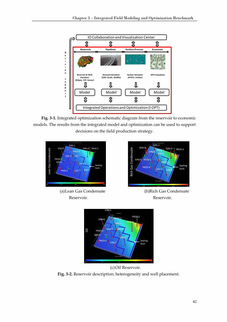
Chapter 3 – Integrated Field Modeling and Optimization Benchmark
42
Fig. 3-1. Integrated optimization schematic diagram from the reservoir to economic
models. The results from the integrated model and optimization can be used to support decisions on the field production strategy.
(a) Lean Gas Condensate
Reservoir. (b)Rich Gas Condensate
Reservoir.
(c) Oil Reservoir.
Fig. 3-2. Reservoir description; heterogeneity and well placement.
Reservoir Pipelines Surface Process Economic
Reservoir & Well Simulator
(Eclipse, VIP, Sensor)
Network Simulator(GAP, OLGA, Wellflo)
Surface Simulator(HYSYS, UniSim)
NPV Calculation
Model Model Model Model
Decision
support
IO Collaboration and Visualization Center
Integrated Operations and Optimization (I-OPT)
Lean
Gas
Con
dens
ate
Sealing fault
PROD 3GINJ 4
GINJ 3
PROD 1
GINJ 1
PROD 2
GINJ 2
GINJ 7PROD 4
GINJ 6PROD 5
GINJ 8
GINJ 5
Rich
Gas
Con
dens
ate
Sealing fault
PROD 3GINJ 4
GINJ 3
PROD 1
GINJ 1PROD 2
GINJ 2
GINJ 7PROD 4
GINJ 6 PROD 5
GINJ 8
GINJ 5
Sealing faultGINJ 7
GINJ 6
GINJ 8
GINJ 5
GINJ 3
GINJ 1
GINJ 2
GINJ 4
PROD 3
PROD 1
PROD 2
PROD 4
PROD 5Oil
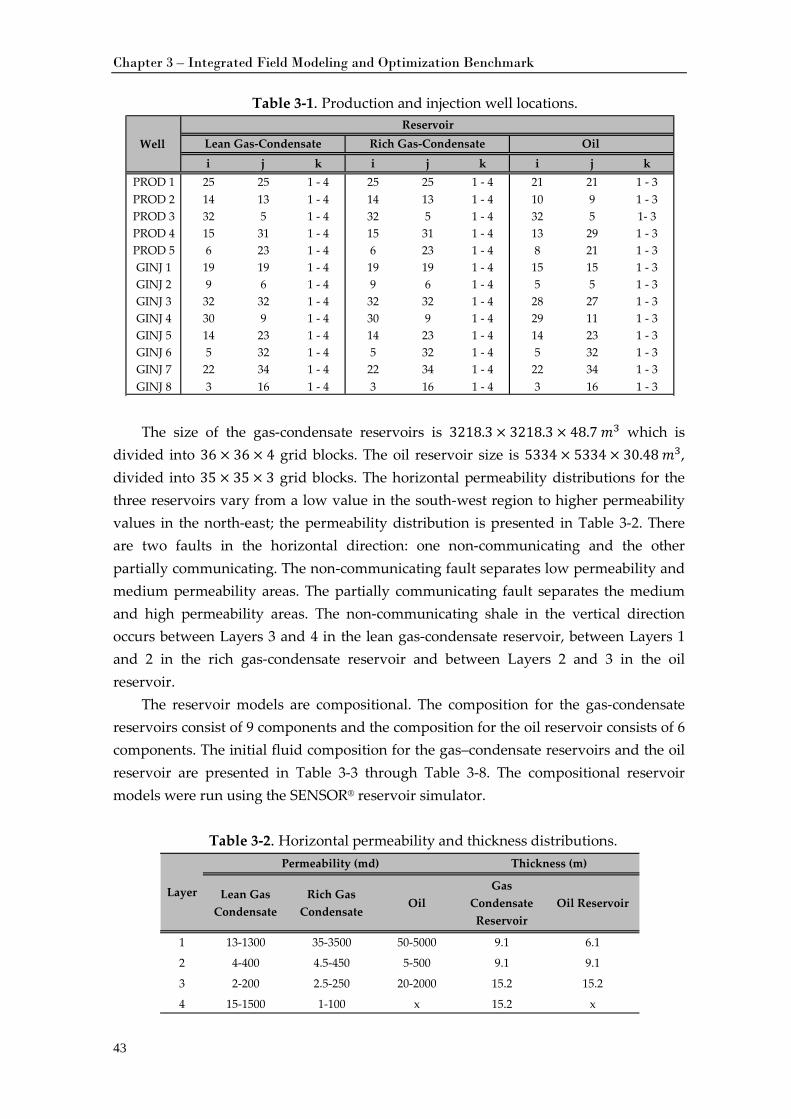
Chapter 3 – Integrated Field Modeling and Optimization Benchmark
43
Table 3-1. Production and injection well locations.
The size of the gas-condensate reservoirs is 3218.3 × 3218.3 × 48.7 𝑚3 which is
divided into 36 × 36 × 4 grid blocks. The oil reservoir size is 5334 × 5334 × 30.48 𝑚3, divided into 35 × 35 × 3 grid blocks. The horizontal permeability distributions for the three reservoirs vary from a low value in the south-west region to higher permeability values in the north-east; the permeability distribution is presented in Table 3-2. There are two faults in the horizontal direction: one non-communicating and the other partially communicating. The non-communicating fault separates low permeability and medium permeability areas. The partially communicating fault separates the medium and high permeability areas. The non-communicating shale in the vertical direction occurs between Layers 3 and 4 in the lean gas-condensate reservoir, between Layers 1 and 2 in the rich gas-condensate reservoir and between Layers 2 and 3 in the oil reservoir.
The reservoir models are compositional. The composition for the gas-condensate reservoirs consist of 9 components and the composition for the oil reservoir consists of 6 components. The initial fluid composition for the gas–condensate reservoirs and the oil reservoir are presented in Table 3-3 through Table 3-8. The compositional reservoir models were run using the SENSOR® reservoir simulator.
Table 3-2. Horizontal permeability and thickness distributions.
i j k i j k i j kPROD 1 25 25 1 - 4 25 25 1 - 4 21 21 1 - 3PROD 2 14 13 1 - 4 14 13 1 - 4 10 9 1 - 3PROD 3 32 5 1 - 4 32 5 1 - 4 32 5 1- 3PROD 4 15 31 1 - 4 15 31 1 - 4 13 29 1 - 3PROD 5 6 23 1 - 4 6 23 1 - 4 8 21 1 - 3GINJ 1 19 19 1 - 4 19 19 1 - 4 15 15 1 - 3GINJ 2 9 6 1 - 4 9 6 1 - 4 5 5 1 - 3GINJ 3 32 32 1 - 4 32 32 1 - 4 28 27 1 - 3GINJ 4 30 9 1 - 4 30 9 1 - 4 29 11 1 - 3GINJ 5 14 23 1 - 4 14 23 1 - 4 14 23 1 - 3GINJ 6 5 32 1 - 4 5 32 1 - 4 5 32 1 - 3GINJ 7 22 34 1 - 4 22 34 1 - 4 22 34 1 - 3GINJ 8 3 16 1 - 4 3 16 1 - 4 3 16 1 - 3
Well Reservoir
Lean Gas-Condensate Rich Gas-Condensate Oil
Lean Gas Condensate
Rich Gas Condensate
OilGas
Condensate Reservoir
Oil Reservoir
1 13-1300 35-3500 50-5000 9.1 6.1
2 4-400 4.5-450 5-500 9.1 9.1
3 2-200 2.5-250 20-2000 15.2 15.2
4 15-1500 1-100 x 15.2 x
Layer
Permeability (md) Thickness (m)
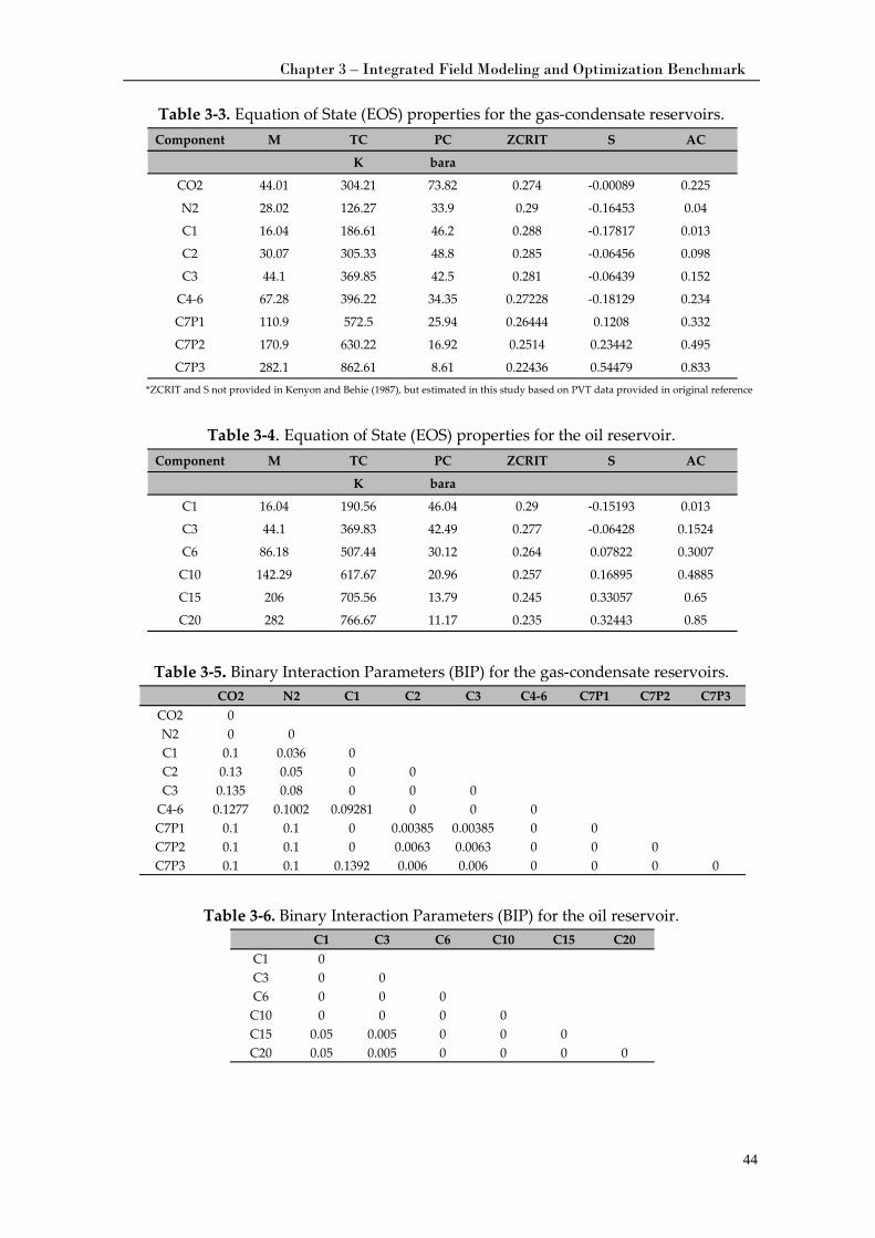
Chapter 3 – Integrated Field Modeling and Optimization Benchmark
44
Table 3-3. Equation of State (EOS) properties for the gas-condensate reservoirs.
*ZCRIT and S not provided in Kenyon and Behie (1987), but estimated in this study based on PVT data provided in original reference
Table 3-4. Equation of State (EOS) properties for the oil reservoir.
Table 3-5. Binary Interaction Parameters (BIP) for the gas-condensate reservoirs.
Table 3-6. Binary Interaction Parameters (BIP) for the oil reservoir.
Component M TC PC ZCRIT S AC
K bara
CO2 44.01 304.21 73.82 0.274 -0.00089 0.225
N2 28.02 126.27 33.9 0.29 -0.16453 0.04
C1 16.04 186.61 46.2 0.288 -0.17817 0.013
C2 30.07 305.33 48.8 0.285 -0.06456 0.098
C3 44.1 369.85 42.5 0.281 -0.06439 0.152
C4-6 67.28 396.22 34.35 0.27228 -0.18129 0.234
C7P1 110.9 572.5 25.94 0.26444 0.1208 0.332
C7P2 170.9 630.22 16.92 0.2514 0.23442 0.495
C7P3 282.1 862.61 8.61 0.22436 0.54479 0.833
Component M TC PC ZCRIT S AC
K bara
C1 16.04 190.56 46.04 0.29 -0.15193 0.013
C3 44.1 369.83 42.49 0.277 -0.06428 0.1524
C6 86.18 507.44 30.12 0.264 0.07822 0.3007
C10 142.29 617.67 20.96 0.257 0.16895 0.4885
C15 206 705.56 13.79 0.245 0.33057 0.65
C20 282 766.67 11.17 0.235 0.32443 0.85
CO2 N2 C1 C2 C3 C4-6 C7P1 C7P2 C7P3CO2 0N2 0 0C1 0.1 0.036 0C2 0.13 0.05 0 0C3 0.135 0.08 0 0 0
C4-6 0.1277 0.1002 0.09281 0 0 0C7P1 0.1 0.1 0 0.00385 0.00385 0 0C7P2 0.1 0.1 0 0.0063 0.0063 0 0 0C7P3 0.1 0.1 0.1392 0.006 0.006 0 0 0 0
C1 C3 C6 C10 C15 C20C1 0C3 0 0C6 0 0 0C10 0 0 0 0C15 0.05 0.005 0 0 0C20 0.05 0.005 0 0 0 0
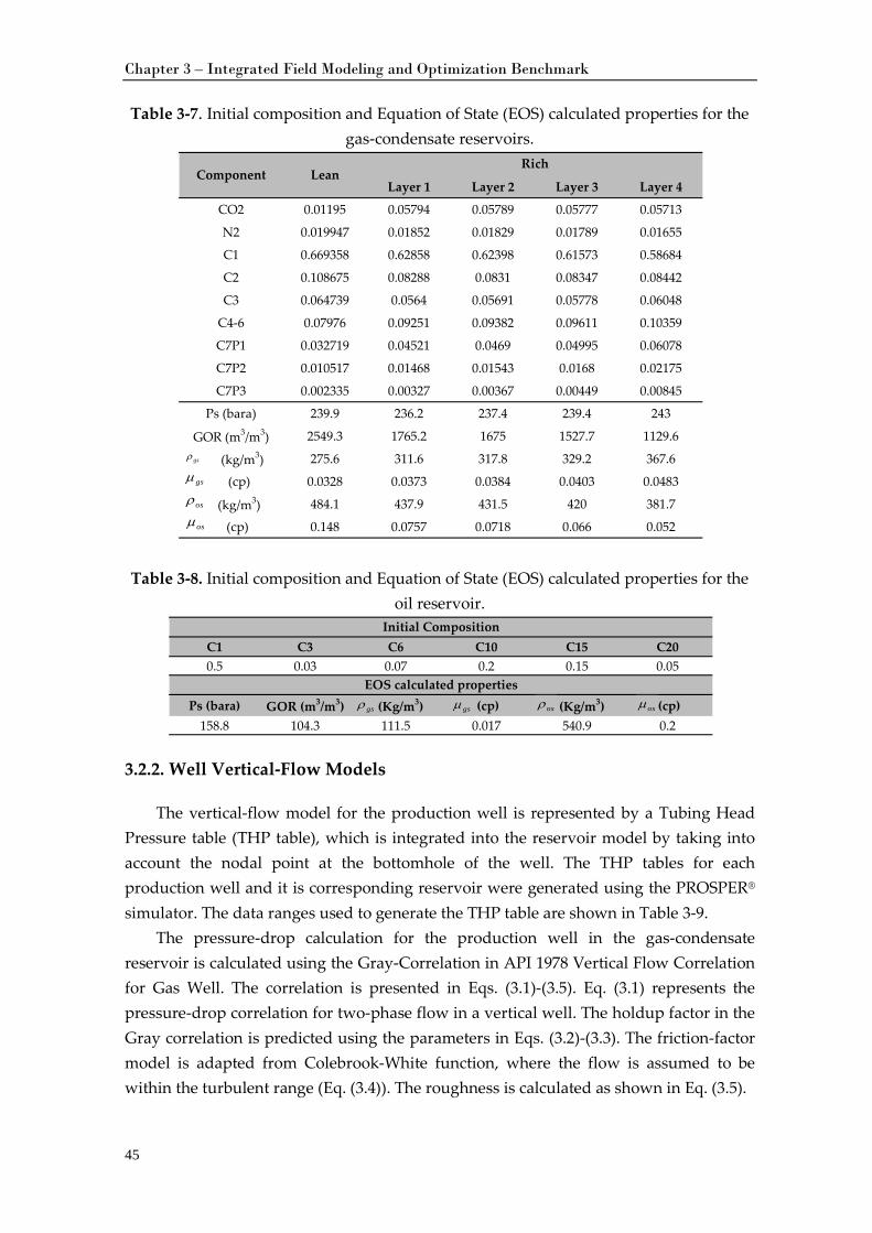
Chapter 3 – Integrated Field Modeling and Optimization Benchmark
45
Table 3-7. Initial composition and Equation of State (EOS) calculated properties for the gas-condensate reservoirs.
Table 3-8. Initial composition and Equation of State (EOS) calculated properties for the oil reservoir.
3.2.2. Well Vertical-Flow Models
The vertical-flow model for the production well is represented by a Tubing Head Pressure table (THP table), which is integrated into the reservoir model by taking into account the nodal point at the bottomhole of the well. The THP tables for each production well and it is corresponding reservoir were generated using the PROSPER® simulator. The data ranges used to generate the THP table are shown in Table 3-9.
The pressure-drop calculation for the production well in the gas-condensate reservoir is calculated using the Gray-Correlation in API 1978 Vertical Flow Correlation for Gas Well. The correlation is presented in Eqs. (3.1)-(3.5). Eq. (3.1) represents the pressure-drop correlation for two-phase flow in a vertical well. The holdup factor in the Gray correlation is predicted using the parameters in Eqs. (3.2)-(3.3). The friction-factor model is adapted from Colebrook-White function, where the flow is assumed to be within the turbulent range (Eq. (3.4)). The roughness is calculated as shown in Eq. (3.5).
Layer 1 Layer 2 Layer 3 Layer 4
CO2 0.01195 0.05794 0.05789 0.05777 0.05713
N2 0.019947 0.01852 0.01829 0.01789 0.01655
C1 0.669358 0.62858 0.62398 0.61573 0.58684
C2 0.108675 0.08288 0.0831 0.08347 0.08442
C3 0.064739 0.0564 0.05691 0.05778 0.06048
C4-6 0.07976 0.09251 0.09382 0.09611 0.10359
C7P1 0.032719 0.04521 0.0469 0.04995 0.06078
C7P2 0.010517 0.01468 0.01543 0.0168 0.02175
C7P3 0.002335 0.00327 0.00367 0.00449 0.00845
Ps (bara) 239.9 236.2 237.4 239.4 243
GOR (m3/m3) 2549.3 1765.2 1675 1527.7 1129.6
(kg/m3) 275.6 311.6 317.8 329.2 367.6
(cp) 0.0328 0.0373 0.0384 0.0403 0.0483
(kg/m3) 484.1 437.9 431.5 420 381.7
(cp) 0.148 0.0757 0.0718 0.066 0.052
Component LeanRich
gsρ
osρgsµ
osµ
C1 C3 C6 C10 C15 C200.5 0.03 0.07 0.2 0.15 0.05
Ps (bara) GOR (m3/m3) (Kg/m3) (cp) (Kg/m3) (cp)158.8 104.3 111.5 0.017 540.9 0.2
Initial Composition
EOS calculated properties
gsρ gsµ osρ osµ
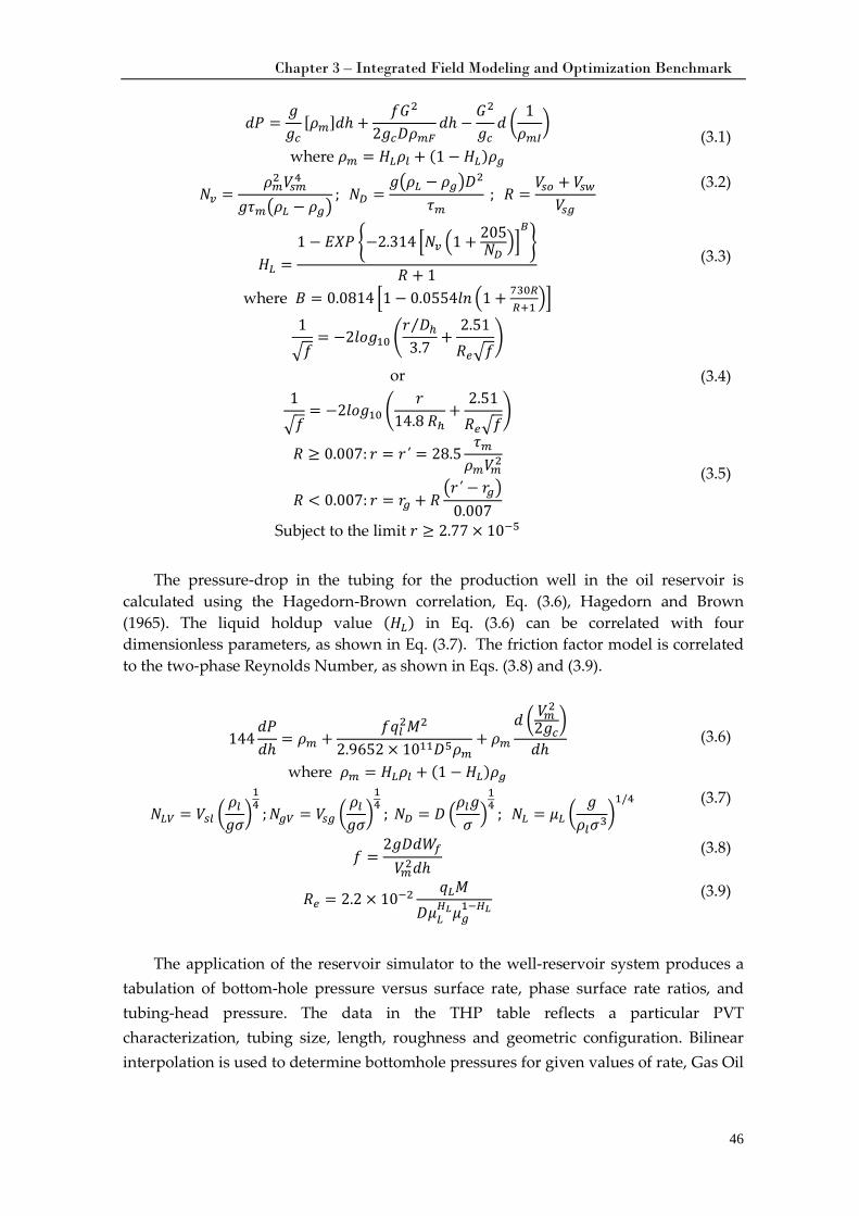
Chapter 3 – Integrated Field Modeling and Optimization Benchmark
46
𝑑𝑑𝑃𝑃 =𝑔𝑔𝑔𝑔𝑐
[𝜌𝑚]𝑑𝑑ℎ +𝑓𝐺2
2𝑔𝑔𝑐𝐷𝐷𝜌𝑚𝐹𝑑𝑑ℎ −
𝐺2
𝑔𝑔𝑐𝑑𝑑 �
1𝜌𝑚𝐼
�
where 𝜌𝑚 = 𝐻𝐿𝜌𝑙 + (1 −𝐻𝐿)𝜌𝑔
(3.1)
𝑁𝑁𝑣 =𝜌𝑚2 𝑉𝑠𝑚4
𝑔𝑔𝜏𝑚�𝜌𝐿 − 𝜌𝑔�; 𝑁𝑁𝐷 =
𝑔𝑔�𝜌𝐿 − 𝜌𝑔�𝐷𝐷2
𝜏𝑚 ; 𝑅 =
𝑉𝑠𝑜 + 𝑉𝑠𝑤𝑉𝑠𝑔
(3.2)
𝐻𝐿 =1 − 𝐸𝑋𝑃𝑃 �−2.314 �𝑁𝑁𝑣 �1 + 205
𝑁𝑁𝐷��𝐵�
𝑅 + 1
where 𝐵 = 0.0814 �1− 0.0554𝑙𝑙𝑛 �1 + 730𝑅𝑅+1
��
(3.3)
1
�𝑓= −2𝑙𝑙𝑜𝑜𝑔𝑔10 �
𝑟𝑟 𝐷𝐷ℎ⁄3.7
+2.51𝑅𝑒�𝑓
�
or 1
�𝑓= −2𝑙𝑙𝑜𝑜𝑔𝑔10 �
𝑟𝑟14.8 𝑅ℎ
+2.51𝑅𝑒�𝑓
�
(3.4)
𝑅 ≥ 0.007: 𝑟𝑟 = 𝑟𝑟′ = 28.5𝜏𝑚𝜌𝑚𝑉𝑚2
𝑅 < 0.007: 𝑟𝑟 = 𝑟𝑟𝑔 + 𝑅�𝑟𝑟′− 𝑟𝑟𝑔�
0.007
Subject to the limit 𝑟𝑟 ≥ 2.77 × 10⁻⁵
(3.5)
The pressure-drop in the tubing for the production well in the oil reservoir is
calculated using the Hagedorn-Brown correlation, Eq. (3.6), Hagedorn and Brown (1965). The liquid holdup value (𝐻𝐿) in Eq. (3.6) can be correlated with four dimensionless parameters, as shown in Eq. (3.7). The friction factor model is correlated to the two-phase Reynolds Number, as shown in Eqs. (3.8) and (3.9).
144𝑑𝑑𝑃𝑃𝑑𝑑ℎ
= 𝜌𝑚 +𝑓𝑞𝑞𝑙2𝑀2
2.9652 × 10¹¹𝐷𝐷5𝜌𝑚+ 𝜌𝑚
𝑑𝑑 � 𝑉𝑚2
2𝑔𝑔𝑐�
𝑑𝑑ℎ
where 𝜌𝑚 = 𝐻𝐿𝜌𝑙 + (1 −𝐻𝐿)𝜌𝑔
(3.6)
𝑁𝑁𝐿𝑉 = 𝑉𝑠𝑙 �𝜌𝑙𝑔𝑔𝜎�14
;𝑁𝑁𝑔𝑉 = 𝑉𝑠𝑔 �𝜌𝑙𝑔𝑔𝜎�14
; 𝑁𝑁𝐷 = 𝐷𝐷 �𝜌𝑙𝑔𝑔𝜎�14 ; 𝑁𝑁𝐿 = 𝜇𝐿 �
𝑔𝑔𝜌𝑙𝜎3
�1/4
(3.7)
𝑓 =2𝑔𝑔𝐷𝐷𝑑𝑑𝑊𝑓
𝑉𝑚2𝑑𝑑ℎ (3.8)
𝑅𝑒 = 2.2 × 10⁻²𝑞𝑞𝐿𝑀
𝐷𝐷𝜇𝐿𝐻𝐿𝜇𝑔
1−𝐻𝐿 (3.9)
The application of the reservoir simulator to the well-reservoir system produces a
tabulation of bottom-hole pressure versus surface rate, phase surface rate ratios, and tubing-head pressure. The data in the THP table reflects a particular PVT characterization, tubing size, length, roughness and geometric configuration. Bilinear interpolation is used to determine bottomhole pressures for given values of rate, Gas Oil
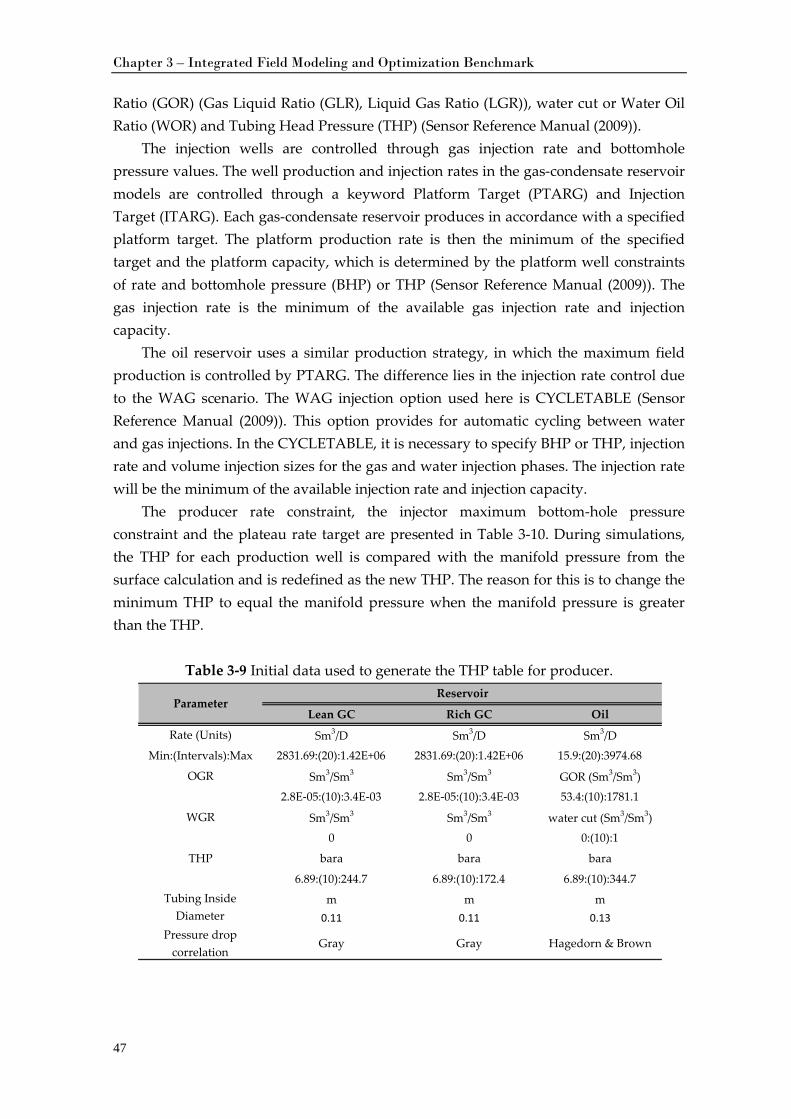
Chapter 3 – Integrated Field Modeling and Optimization Benchmark
47
Ratio (GOR) (Gas Liquid Ratio (GLR), Liquid Gas Ratio (LGR)), water cut or Water Oil Ratio (WOR) and Tubing Head Pressure (THP) (Sensor Reference Manual (2009)).
The injection wells are controlled through gas injection rate and bottomhole pressure values. The well production and injection rates in the gas-condensate reservoir models are controlled through a keyword Platform Target (PTARG) and Injection Target (ITARG). Each gas-condensate reservoir produces in accordance with a specified platform target. The platform production rate is then the minimum of the specified target and the platform capacity, which is determined by the platform well constraints of rate and bottomhole pressure (BHP) or THP (Sensor Reference Manual (2009)). The gas injection rate is the minimum of the available gas injection rate and injection capacity.
The oil reservoir uses a similar production strategy, in which the maximum field production is controlled by PTARG. The difference lies in the injection rate control due to the WAG scenario. The WAG injection option used here is CYCLETABLE (Sensor Reference Manual (2009)). This option provides for automatic cycling between water and gas injections. In the CYCLETABLE, it is necessary to specify BHP or THP, injection rate and volume injection sizes for the gas and water injection phases. The injection rate will be the minimum of the available injection rate and injection capacity.
The producer rate constraint, the injector maximum bottom-hole pressure constraint and the plateau rate target are presented in Table 3-10. During simulations, the THP for each production well is compared with the manifold pressure from the surface calculation and is redefined as the new THP. The reason for this is to change the minimum THP to equal the manifold pressure when the manifold pressure is greater than the THP.
Table 3-9 Initial data used to generate the THP table for producer.
Lean GC Rich GC Oil
Rate (Units) Sm3/D Sm3/D Sm3/D
Min:(Intervals):Max 2831.69:(20):1.42E+06 2831.69:(20):1.42E+06 15.9:(20):3974.68
OGR Sm3/Sm3 Sm3/Sm3 GOR (Sm3/Sm3)
2.8E-05:(10):3.4E-03 2.8E-05:(10):3.4E-03 53.4:(10):1781.1
WGR Sm3/Sm3 Sm3/Sm3 water cut (Sm3/Sm3)
0 0 0:(10):1
THP bara bara bara
6.89:(10):244.7 6.89:(10):172.4 6.89:(10):344.7
m m m0.11 0.11 0.13
Pressure drop correlation
Gray Gray Hagedorn & Brown
Tubing Inside Diameter
ParameterReservoir
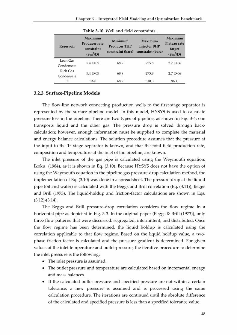
Chapter 3 – Integrated Field Modeling and Optimization Benchmark
48
Table 3-10. Well and field constraints.
3.2.3. Surface-Pipeline Models
The flow-line network connecting production wells to the first-stage separator is represented by the surface-pipeline model. In this model, HYSYS is used to calculate pressure loss in the pipeline. There are two types of pipeline, as shown in Fig. 3-4: one transports liquid and the other gas. The pressure drop is solved through back-calculation; however, enough information must be supplied to complete the material and energy balance calculations. The solution procedure assumes that the pressure at the input to the 1st stage separator is known, and that the total field production rate, composition and temperature at the inlet of the pipeline, are known.
The inlet pressure of the gas pipe is calculated using the Weymouth equation, Ikoku (1984), as it is shown in Eq. (3.10). Because HYSYS does not have the option of using the Waymouth equation in the pipeline gas pressure-drop calculation method, the implementation of Eq. (3.10) was done in a spreadsheet. The pressure-drop at the liquid pipe (oil and water) is calculated with the Beggs and Brill correlation (Eq. (3.11)), Beggs and Brill (1973). The liquid-holdup and friction-factor calculations are shown in Eqs. (3.12)-(3.14).
The Beggs and Brill pressure-drop correlation considers the flow regime in a horizontal pipe as depicted in Fig. 3-3. In the original paper (Beggs & Brill (1973)), only three flow patterns that were discussed: segregated, intermittent, and distributed. Once the flow regime has been determined, the liquid holdup is calculated using the correlation applicable to that flow regime. Based on the liquid holdup value, a two-phase friction factor is calculated and the pressure gradient is determined. For given values of the inlet temperature and outlet pressure, the iterative procedure to determine the inlet pressure is the following:
• The inlet pressure is assumed. • The outlet pressure and temperature are calculated based on incremental energy
and mass balances. • If the calculated outlet pressure and specified pressure are not within a certain
tolerance, a new pressure is assumed and is processed using the same calculation procedure. The iterations are continued until the absolute difference of the calculated and specified pressure is less than a specified tolerance value.
Reservoir
Maximum Producer rate
constraint (Sm3/D)
Minimum Producer THP
constraint (bara)
Maximum Injector BHP
constraint (bara)
Maximum Plateau rate
target (Sm3/D)
Lean Gas Condensate
5.4 E+05 68.9 275.8 2.7 E+06
Rich Gas Condensate
5.4 E+05 68.9 275.8 2.7 E+06
Oil 1920 68.9 310.3 9600
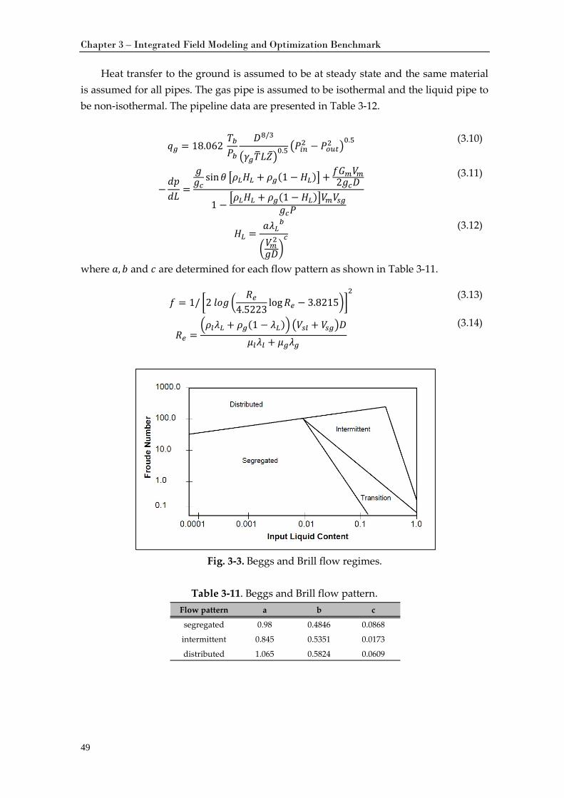
Chapter 3 – Integrated Field Modeling and Optimization Benchmark
49
Heat transfer to the ground is assumed to be at steady state and the same material is assumed for all pipes. The gas pipe is assumed to be isothermal and the liquid pipe to be non-isothermal. The pipeline data are presented in Table 3-12.
𝑞𝑞𝑔 = 18.062 𝑇𝑇𝑏𝑃𝑃𝑏
𝐷𝐷8/3
�𝛾𝑔𝑇𝑇�𝐿𝐿�̅��0.5 �𝑃𝑃𝑖𝑛
2 − 𝑃𝑃𝑜𝑢𝑡2 �0.5 (3.10)
−𝑑𝑑𝑠𝑠𝑑𝑑𝐿𝐿
=
𝑔𝑔𝑔𝑔𝑐
sin𝜃 �𝜌𝐿𝐻𝐿 + 𝜌𝑔(1 −𝐻𝐿)�+ 𝑓𝐺𝑚𝑉𝑚2𝑔𝑔𝑐𝐷𝐷
1 −�𝜌𝐿𝐻𝐿 + 𝜌𝑔(1 −𝐻𝐿)�𝑉𝑚𝑉𝑠𝑔
𝑔𝑔𝑐𝑃𝑃
(3.11)
𝐻𝐿 =𝑎𝜆𝐿
𝑏
�𝑉𝑚2
𝑔𝑔𝐷𝐷�𝑐
(3.12)
where 𝑎, 𝑏 and 𝑐 are determined for each flow pattern as shown in Table 3-11.
𝑓 = 1/ �2 𝑙𝑙𝑜𝑜𝑔𝑔 �𝑅𝑒
4.5223log𝑅𝑒 − 3.8215��
2
(3.13)
𝑅𝑒 =�𝜌𝑙𝜆𝐿 + 𝜌𝑔(1 − 𝜆𝐿)� �𝑉𝑠𝑙 + 𝑉𝑠𝑔�𝐷𝐷
𝜇𝑙𝜆𝑙 + 𝜇𝑔𝜆𝑔
(3.14)
Fig. 3-3. Beggs and Brill flow regimes.
Table 3-11. Beggs and Brill flow pattern.
Flow pattern a b c
segregated 0.98 0.4846 0.0868
intermittent 0.845 0.5351 0.0173
distributed 1.065 0.5824 0.0609
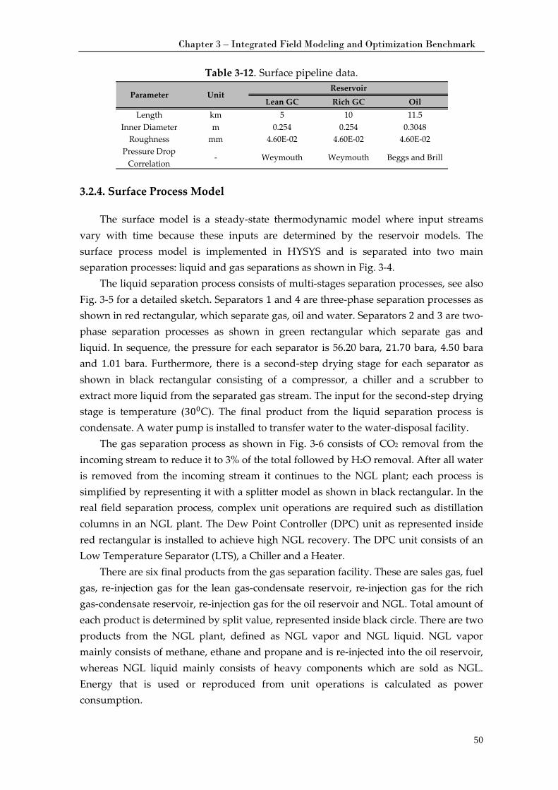
Chapter 3 – Integrated Field Modeling and Optimization Benchmark
50
Table 3-12. Surface pipeline data.
3.2.4. Surface Process Model
The surface model is a steady-state thermodynamic model where input streams vary with time because these inputs are determined by the reservoir models. The surface process model is implemented in HYSYS and is separated into two main separation processes: liquid and gas separations as shown in Fig. 3-4.
The liquid separation process consists of multi-stages separation processes, see also Fig. 3-5 for a detailed sketch. Separators 1 and 4 are three-phase separation processes as shown in red rectangular, which separate gas, oil and water. Separators 2 and 3 are two-phase separation processes as shown in green rectangular which separate gas and liquid. In sequence, the pressure for each separator is 56.20 bara, 21.70 bara, 4.50 bara and 1.01 bara. Furthermore, there is a second-step drying stage for each separator as shown in black rectangular consisting of a compressor, a chiller and a scrubber to extract more liquid from the separated gas stream. The input for the second-step drying stage is temperature (300C). The final product from the liquid separation process is condensate. A water pump is installed to transfer water to the water-disposal facility.
The gas separation process as shown in Fig. 3-6 consists of CO2 removal from the incoming stream to reduce it to 3% of the total followed by H2O removal. After all water is removed from the incoming stream it continues to the NGL plant; each process is simplified by representing it with a splitter model as shown in black rectangular. In the real field separation process, complex unit operations are required such as distillation columns in an NGL plant. The Dew Point Controller (DPC) unit as represented inside red rectangular is installed to achieve high NGL recovery. The DPC unit consists of an Low Temperature Separator (LTS), a Chiller and a Heater.
There are six final products from the gas separation facility. These are sales gas, fuel gas, re-injection gas for the lean gas-condensate reservoir, re-injection gas for the rich gas-condensate reservoir, re-injection gas for the oil reservoir and NGL. Total amount of each product is determined by split value, represented inside black circle. There are two products from the NGL plant, defined as NGL vapor and NGL liquid. NGL vapor mainly consists of methane, ethane and propane and is re-injected into the oil reservoir, whereas NGL liquid mainly consists of heavy components which are sold as NGL. Energy that is used or reproduced from unit operations is calculated as power consumption.
Lean GC Rich GC OilLength km 5 10 11.5
Inner Diameter m 0.254 0.254 0.3048Roughness mm 4.60E-02 4.60E-02 4.60E-02
Pressure Drop Correlation
- Weymouth Weymouth Beggs and Brill
Parameter UnitReservoir
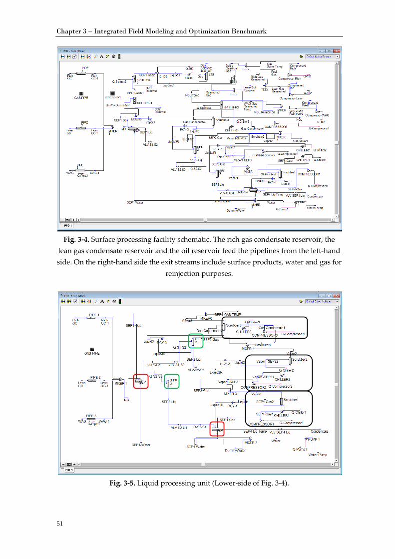
Chapter 3 – Integrated Field Modeling and Optimization Benchmark
51
Fig. 3-4. Surface processing facility schematic. The rich gas condensate reservoir, the
lean gas condensate reservoir and the oil reservoir feed the pipelines from the left-hand side. On the right-hand side the exit streams include surface products, water and gas for
reinjection purposes.
Fig. 3-5. Liquid processing unit (Lower-side of Fig. 3-4).
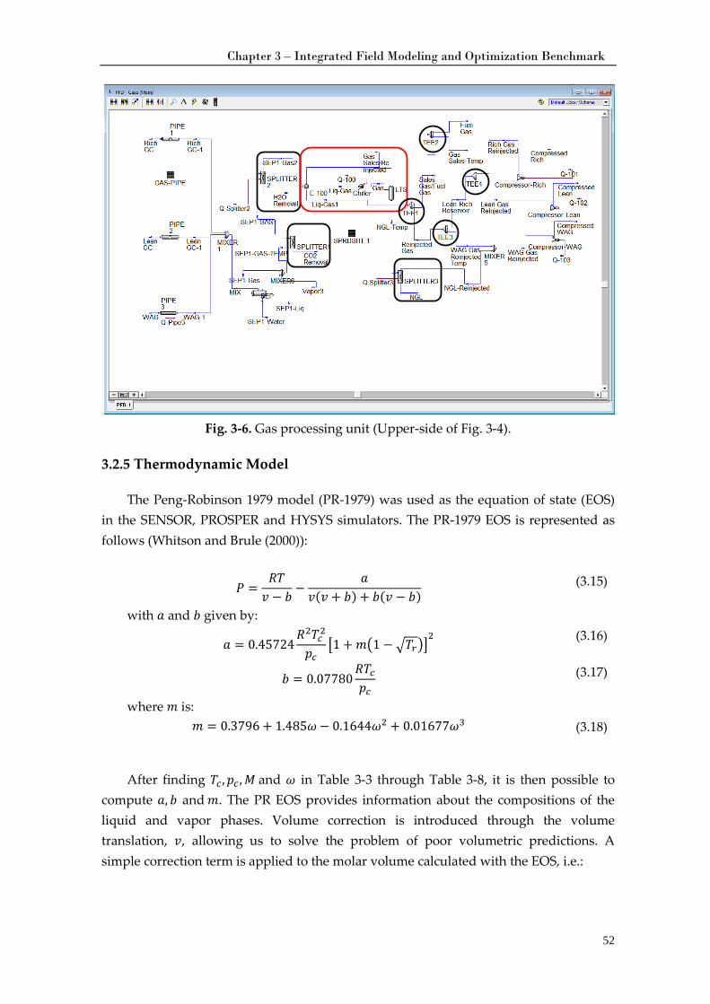
Chapter 3 – Integrated Field Modeling and Optimization Benchmark
52
Fig. 3-6. Gas processing unit (Upper-side of Fig. 3-4).
3.2.5 Thermodynamic Model
The Peng-Robinson 1979 model (PR-1979) was used as the equation of state (EOS) in the SENSOR, PROSPER and HYSYS simulators. The PR-1979 EOS is represented as follows (Whitson and Brule (2000)):
𝑃𝑃 =𝑅𝑇𝑇𝑣 − 𝑏
−𝑎
𝑣(𝑣 + 𝑏) + 𝑏(𝑣 − 𝑏) (3.15)
with 𝑎 and 𝑏 given by:
𝑎 = 0.45724𝑅2𝑇𝑇𝑐2
𝑠𝑠𝑐�1 + 𝑚�1 −�𝑇𝑇𝑟��
2
(3.16)
𝑏 = 0.07780𝑅𝑇𝑇𝑐𝑠𝑠𝑐
(3.17)
where 𝑚 is: 𝑚 = 0.3796 + 1.485𝜔− 0.1644𝜔2 + 0.01677𝜔3 (3.18)
After finding 𝑇𝑇𝑐 ,𝑠𝑠𝑐 ,𝑀 and 𝜔 in Table 3-3 through Table 3-8, it is then possible to
compute 𝑎, 𝑏 and 𝑚. The PR EOS provides information about the compositions of the liquid and vapor phases. Volume correction is introduced through the volume translation, 𝑣, allowing us to solve the problem of poor volumetric predictions. A simple correction term is applied to the molar volume calculated with the EOS, i.e.:
Chapter 3 – Integrated Field Modeling and Optimization Benchmark
53
𝑣𝑙 = 𝑣𝑙𝐸𝑂𝑆 −�𝑥𝑐𝑐𝑐
𝑁
𝑐=1
(3.19)
𝑣𝑔 = 𝑣𝑔𝐸𝑂𝑆 −�𝑦𝑐𝑐𝑐
𝑁
𝑐=1
(3.20)
PhazeComp® as a PVT simulator was used to generate PVT information and
compared with HYSYS. The only difference in EOS input parameters was the volume shift factors where HYSYS (incorrectly) requires the negative of the actual value.
3.2.6. Economic Model
The goal of the integrated model is to study field asset value as represented by an economic model. This model is based on Net Present Value (NPV), which is calculated in the usual manner by introducing a discount factor. The operational expenses (OPEX) are defined by a fixed amount. The OPEX covers the pipeline and well operating costs and was estimated at around one million USD per day for the base case.
The field revenue is obtained from gas, NGL and condensate sales. The daily cost is summed from the volume of water production and injection, CO2 removal and power consumption. For the base case the initial condensate and NGL prices used were 503 USD/m3 (80 USD/bbl), the initial gas price was 0.21 USD/m3 (6 USD/Mcf), the initial water production and injection cost was 18.4 USD/m3 (2.93 USD/bbl), the initial CO2
removal cost was 15.4 USD/MT, and the initial power cost was 5 cents/kWh. Previously, NPV was calculated as a function of project time step (PTS), ∆𝑡𝑝, as
shown in Eqs. (3.21)-(3.22). 𝑅𝑐(𝑡) is average cash flow per PTS and 𝑁𝑁 is total simulation time divided by PTS. We found that the calculation was incorrect, as shown in Fig. 3-7. The NPV kept increasing as PTS was decreased. An error was found in the NPV calculation basis, as shown in Fig. 3-8. The red line in the figure shows the revenue in USD per day for a PTS 1095 days (3 years). The gray line represents an NPV calculation for each PTS while the black line is the NPV calculation on an annual basis. The different ways of calculating NPV resulted in significantly different final NPV results.
The NPV calculation was thus corrected using Eqs. (3.23)-(3.24). Here, 𝑅𝑐(Δ𝑡𝑁𝑃𝑉)�������������� is the average annual cash flow, where ∆𝑡𝑁𝑃𝑉 is always 365 days (1 Year) and 𝑁𝑁 = 20. The total simulation is 20 years. In the new formulation, the NPV is calculated on an annual basis and 𝐽𝑁𝑃𝑉 does not depend on the PTS. The new formulation gave better results for different PTS values as shown in Fig. 3-7. The NPV here approaches the actual value as the PTS is decreased.
𝑅𝑐(𝑡) = �𝑞𝑞𝑔(𝑡)𝑟𝑟𝑔 + 𝑞𝑞𝑐(𝑡)𝑟𝑟𝑐 + 𝑞𝑞𝑁𝐺𝐿(𝑡)𝑟𝑟𝑁𝐺𝐿 − �𝑞𝑞𝑤𝑖(𝑡) + 𝑞𝑞𝑤𝑝(𝑡)� 𝑟𝑟𝑤 − 𝑠𝑠(𝑡)𝑟𝑟𝑝
− 𝑀𝐶𝑂2(𝑡)𝑟𝑟𝐶𝑂2�
(3.21)
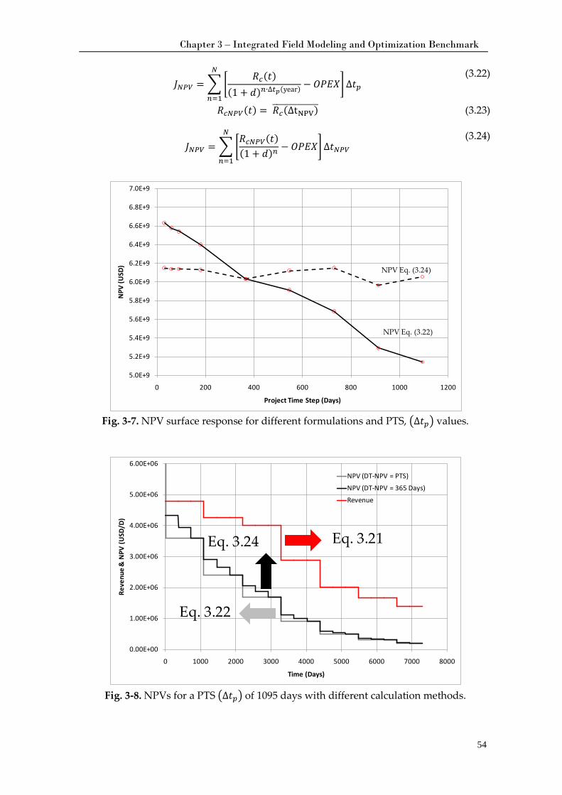
Chapter 3 – Integrated Field Modeling and Optimization Benchmark
54
𝐽𝑁𝑃𝑉 = ��𝑅𝑐(𝑡)
(1 + 𝑑𝑑)𝑛∙∆𝑡𝑝(year) − 𝑂𝑃𝑃𝐸𝑋� ∆𝑡𝑝
𝑁
𝑛=1
(3.22)
𝑅𝑐𝑁𝑃𝑉(𝑡) = 𝑅𝑐(∆tNPV)������������� (3.23)
𝐽𝑁𝑃𝑉 = ��𝑅𝑐𝑁𝑃𝑉(𝑡)(1 + 𝑑𝑑)𝑛 − 𝑂𝑃𝑃𝐸𝑋� ∆𝑡𝑁𝑃𝑉
𝑁
𝑛=1
(3.24)
Fig. 3-7. NPV surface response for different formulations and PTS, �∆𝑡𝑝� values.
Fig. 3-8. NPVs for a PTS �∆𝑡𝑝� of 1095 days with different calculation methods.
5.0E+9
5.2E+9
5.4E+9
5.6E+9
5.8E+9
6.0E+9
6.2E+9
6.4E+9
6.6E+9
6.8E+9
7.0E+9
0 200 400 600 800 1000 1200
NPV
(USD
)
Project Time Step (Days)
NPV Eq. (3.22)
NPV Eq. (3.24)
0.00E+00
1.00E+06
2.00E+06
3.00E+06
4.00E+06
5.00E+06
6.00E+06
0 1000 2000 3000 4000 5000 6000 7000 8000
Reve
nue
& N
PV (U
SD/D
)
Time (Days)
NPV (DT-NPV = PTS)
NPV (DT-NPV = 365 Days)
Revenue
Eq. 3.21Eq. 3.24
Eq. 3.22
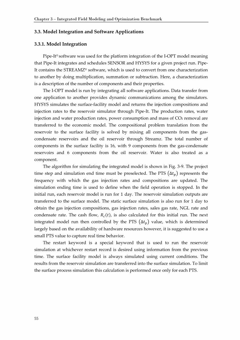
Chapter 3 – Integrated Field Modeling and Optimization Benchmark
55
3.3. Model Integration and Software Applications
3.3.1. Model Integration
Pipe-It® software was used for the platform integration of the I-OPT model meaning that Pipe-It integrates and schedules SENSOR and HYSYS for a given project run. Pipe-It contains the STREAMZ® software, which is used to convert from one characterization to another by doing multiplication, summation or subtraction. Here, a characterization is a description of the number of components and their properties.
The I-OPT model is run by integrating all software applications. Data transfer from one application to another provides dynamic communications among the simulators. HYSYS simulates the surface-facility model and returns the injection compositions and injection rates to the reservoir simulator through Pipe-It. The production rates, water injection and water production rates, power consumption and mass of CO2 removal are transferred to the economic model. The compositional problem translation from the reservoir to the surface facility is solved by mixing all components from the gas-condensate reservoirs and the oil reservoir through Streamz. The total number of components in the surface facility is 16, with 9 components from the gas-condensate reservoirs and 6 components from the oil reservoir. Water is also treated as a component.
The algorithm for simulating the integrated model is shown in Fig. 3-9. The project time step and simulation end time must be preselected. The PTS �∆𝑡𝑝� represents the frequency with which the gas injection rates and compositions are updated. The simulation ending time is used to define when the field operation is stopped. In the initial run, each reservoir model is run for 1 day. The reservoir simulation outputs are transferred to the surface model. The static surface simulation is also run for 1 day to obtain the gas injection compositions, gas injection rates, sales gas rate, NGL rate and condensate rate. The cash flow, 𝑅𝑐(𝑡), is also calculated for this initial run. The next integrated model run then controlled by the PTS �∆𝑡𝑝� value, which is determined largely based on the availability of hardware resources however, it is suggested to use a small PTS value to capture real time behavior.
The restart keyword is a special keyword that is used to run the reservoir simulation at whichever restart record is desired using information from the previous time. The surface facility model is always simulated using current conditions. The results from the reservoir simulation are transferred into the surface simulation. To limit the surface process simulation this calculation is performed once only for each PTS.
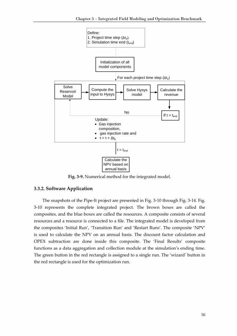
Chapter 3 – Integrated Field Modeling and Optimization Benchmark
56
Fig. 3-9. Numerical method for the integrated model.
3.3.2. Software Application
The snapshots of the Pipe-It project are presented in Fig. 3-10 through Fig. 3-14. Fig. 3-10 represents the complete integrated project. The brown boxes are called the composites, and the blue boxes are called the resources. A composite consists of several resources and a resource is connected to a file. The integrated model is developed from the composites ‘Initial Run’, ‘Transition Run’ and ‘Restart Runs’. The composite ‘NPV’ is used to calculate the NPV on an annual basis. The discount factor calculation and OPEX subtraction are done inside this composite. The ‘Final Results’ composite functions as a data aggregation and collection module at the simulation’s ending time. The green button in the red rectangle is assigned to a single run. The ‘wizard’ button in the red rectangle is used for the optimization run.
Initialization of all model components
Calculate the NPV based on annual basis
Define:1. Project time step (∆tp).2. Simulation time end (tend)
Solve Reservoir
Model
Compute the input to Hysys
If t = tendNo
Solve Hysys model
Update:• Gas injection
composition,• gas injection rate and• t = t + Δtp
Calculate the revenue
For each project time step (∆tp)
t = tend
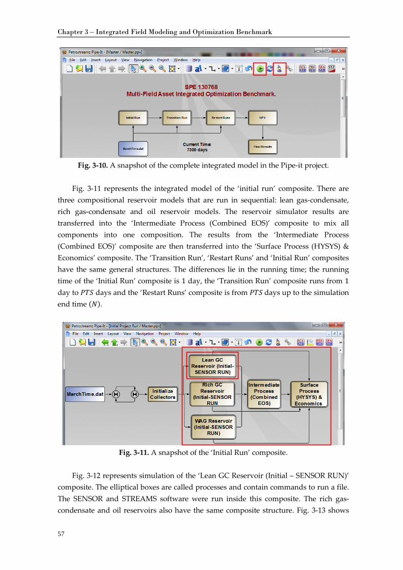
Chapter 3 – Integrated Field Modeling and Optimization Benchmark
57
Fig. 3-10. A snapshot of the complete integrated model in the Pipe-it project.
Fig. 3-11 represents the integrated model of the ‘initial run’ composite. There are
three compositional reservoir models that are run in sequential: lean gas-condensate, rich gas-condensate and oil reservoir models. The reservoir simulator results are transferred into the ‘Intermediate Process (Combined EOS)’ composite to mix all components into one composition. The results from the ‘Intermediate Process (Combined EOS)’ composite are then transferred into the ‘Surface Process (HYSYS) & Economics’ composite. The ‘Transition Run’, ‘Restart Runs’ and ‘Initial Run’ composites have the same general structures. The differences lie in the running time; the running time of the ‘Initial Run’ composite is 1 day, the ‘Transition Run’ composite runs from 1 day to 𝑃𝑃𝑇𝑇𝑆 days and the ‘Restart Runs’ composite is from 𝑃𝑃𝑇𝑇𝑆 days up to the simulation end time (𝑁𝑁).
Fig. 3-11. A snapshot of the ‘Initial Run’ composite.
Fig. 3-12 represents simulation of the ‘Lean GC Reservoir (Initial – SENSOR RUN)’
composite. The elliptical boxes are called processes and contain commands to run a file. The SENSOR and STREAMS software were run inside this composite. The rich gas-condensate and oil reservoirs also have the same composite structure. Fig. 3-13 shows
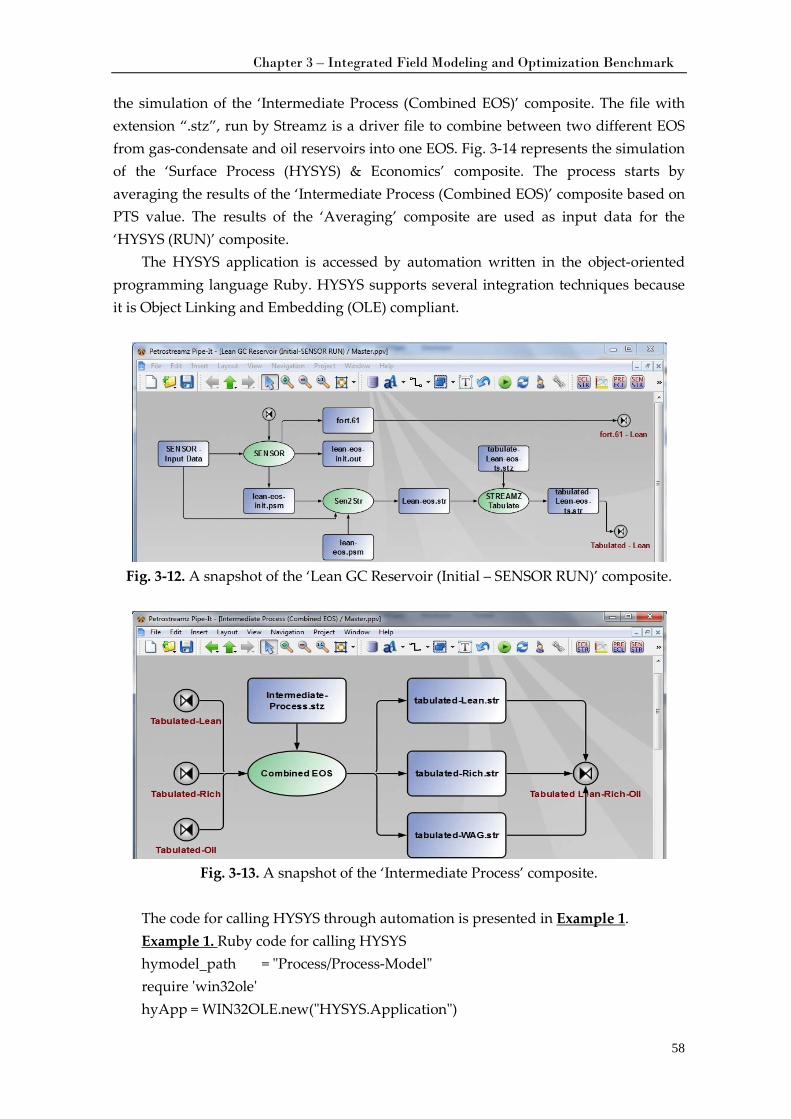
Chapter 3 – Integrated Field Modeling and Optimization Benchmark
58
the simulation of the ‘Intermediate Process (Combined EOS)’ composite. The file with extension “.stz”, run by Streamz is a driver file to combine between two different EOS from gas-condensate and oil reservoirs into one EOS. Fig. 3-14 represents the simulation of the ‘Surface Process (HYSYS) & Economics’ composite. The process starts by averaging the results of the ‘Intermediate Process (Combined EOS)’ composite based on PTS value. The results of the ‘Averaging’ composite are used as input data for the ‘HYSYS (RUN)’ composite.
The HYSYS application is accessed by automation written in the object-oriented programming language Ruby. HYSYS supports several integration techniques because it is Object Linking and Embedding (OLE) compliant.
Fig. 3-12. A snapshot of the ‘Lean GC Reservoir (Initial – SENSOR RUN)’ composite.
Fig. 3-13. A snapshot of the ‘Intermediate Process’ composite.
The code for calling HYSYS through automation is presented in Example 1. Example 1. hymodel_path = "Process/Process-Model"
Ruby code for calling HYSYS
require 'win32ole' hyApp = WIN32OLE.new("HYSYS.Application")
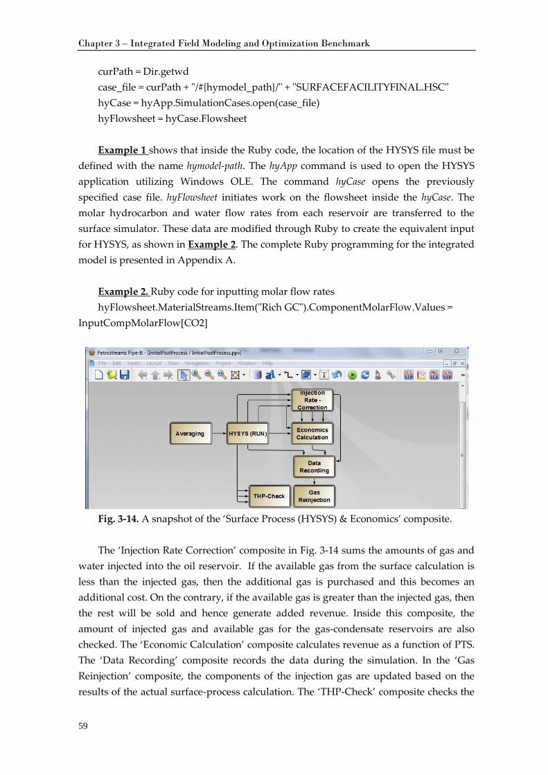
Chapter 3 – Integrated Field Modeling and Optimization Benchmark
59
curPath = Dir.getwd case_file = curPath + "/#{hymodel_path}/" + "SURFACEFACILITYFINAL.HSC" hyCase = hyApp.SimulationCases.open(case_file) hyFlowsheet = hyCase.Flowsheet Example 1 shows that inside the Ruby code, the location of the HYSYS file must be
defined with the name hymodel-path. The hyApp command is used to open the HYSYS application utilizing Windows OLE. The command hyCase opens the previously specified case file. hyFlowsheet initiates work on the flowsheet inside the hyCase. The molar hydrocarbon and water flow rates from each reservoir are transferred to the surface simulator. These data are modified through Ruby to create the equivalent input for HYSYS, as shown in Example 2
. The complete Ruby programming for the integrated model is presented in Appendix A.
Example 2. hyFlowsheet.MaterialStreams.Item("Rich GC").ComponentMolarFlow.Values =
InputCompMolarFlow[CO2]
Ruby code for inputting molar flow rates
Fig. 3-14. A snapshot of the ‘Surface Process (HYSYS) & Economics’ composite. The ‘Injection Rate Correction’ composite in Fig. 3-14 sums the amounts of gas and
water injected into the oil reservoir. If the available gas from the surface calculation is less than the injected gas, then the additional gas is purchased and this becomes an additional cost. On the contrary, if the available gas is greater than the injected gas, then the rest will be sold and hence generate added revenue. Inside this composite, the amount of injected gas and available gas for the gas-condensate reservoirs are also checked. The ‘Economic Calculation’ composite calculates revenue as a function of PTS. The ‘Data Recording’ composite records the data during the simulation. In the ‘Gas Reinjection’ composite, the components of the injection gas are updated based on the results of the actual surface-process calculation. The ‘THP-Check’ composite checks the
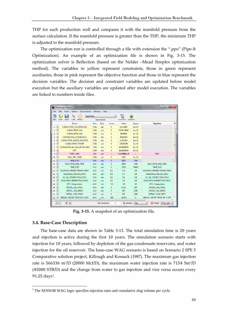
Chapter 3 – Integrated Field Modeling and Optimization Benchmark
60
THP for each production well and compares it with the manifold pressure from the surface calculation. If the manifold pressure is greater than the THP, the minimum THP is adjusted to the manifold pressure.
The optimization run is controlled through a file with extension the “.ppo” (Pipe-It Optimization). An example of an optimization file is shown in Fig. 3-15. The optimization solver is Reflection (based on the Nelder –Mead Simplex optimization method). The variables in yellow represent constraints, those in green represent auxiliaries, those in pink represent the objective function and those in blue represent the decision variables. The decision and constraint variables are updated before model execution but the auxiliary variables are updated after model execution. The variables are linked to numbers inside files.
Fig. 3-15. A snapshot of an optimization file.
3.4. Base-Case Description
The base-case data are shown in Table 3-13. The total simulation time is 20 years and injection is active during the first 10 years. The simulation scenario starts with injection for 10 years, followed by depletion of the gas-condensate reservoirs, and water injection for the oil reservoir. The base-case WAG scenario is based on Scenario 2 SPE 5 Comparative solution project, Killough and Kossack (1987). The maximum gas injection rate is 566336 m3/D (20000 Mcf/D), the maximum water injection rate is 7154 Sm3/D (45000 STB/D) and the change from water to gas injection and vice versa occurs every 91.25 days2
2 The SENSOR WAG logic specifies injection rates and cumulative slug volume per cycle.
.
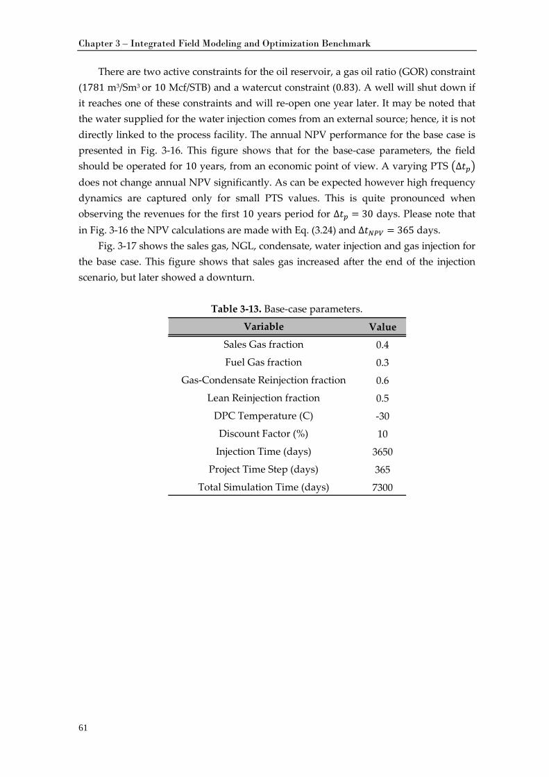
Chapter 3 – Integrated Field Modeling and Optimization Benchmark
61
There are two active constraints for the oil reservoir, a gas oil ratio (GOR) constraint (1781 m3/Sm3 or 10 Mcf/STB) and a watercut constraint (0.83). A well will shut down if it reaches one of these constraints and will re-open one year later. It may be noted that the water supplied for the water injection comes from an external source; hence, it is not directly linked to the process facility. The annual NPV performance for the base case is presented in Fig. 3-16. This figure shows that for the base-case parameters, the field should be operated for 10 years, from an economic point of view. A varying PTS �∆𝑡𝑝� does not change annual NPV significantly. As can be expected however high frequency dynamics are captured only for small PTS values. This is quite pronounced when observing the revenues for the first 10 years period for ∆𝑡𝑝 = 30 days. Please note that in Fig. 3-16 the NPV calculations are made with Eq. (3.24) and ∆𝑡𝑁𝑃𝑉 = 365 days.
Fig. 3-17 shows the sales gas, NGL, condensate, water injection and gas injection for the base case. This figure shows that sales gas increased after the end of the injection scenario, but later showed a downturn.
Table 3-13. Base-case parameters.
Value
0.4
0.3
0.6
0.5
-30
10
3650
365
7300
Discount Factor (%)
Injection Time (days)
Project Time Step (days)
Total Simulation Time (days)
Variable
Sales Gas fraction
Fuel Gas fraction
Gas-Condensate Reinjection fraction
Lean Reinjection fraction
DPC Temperature (C)
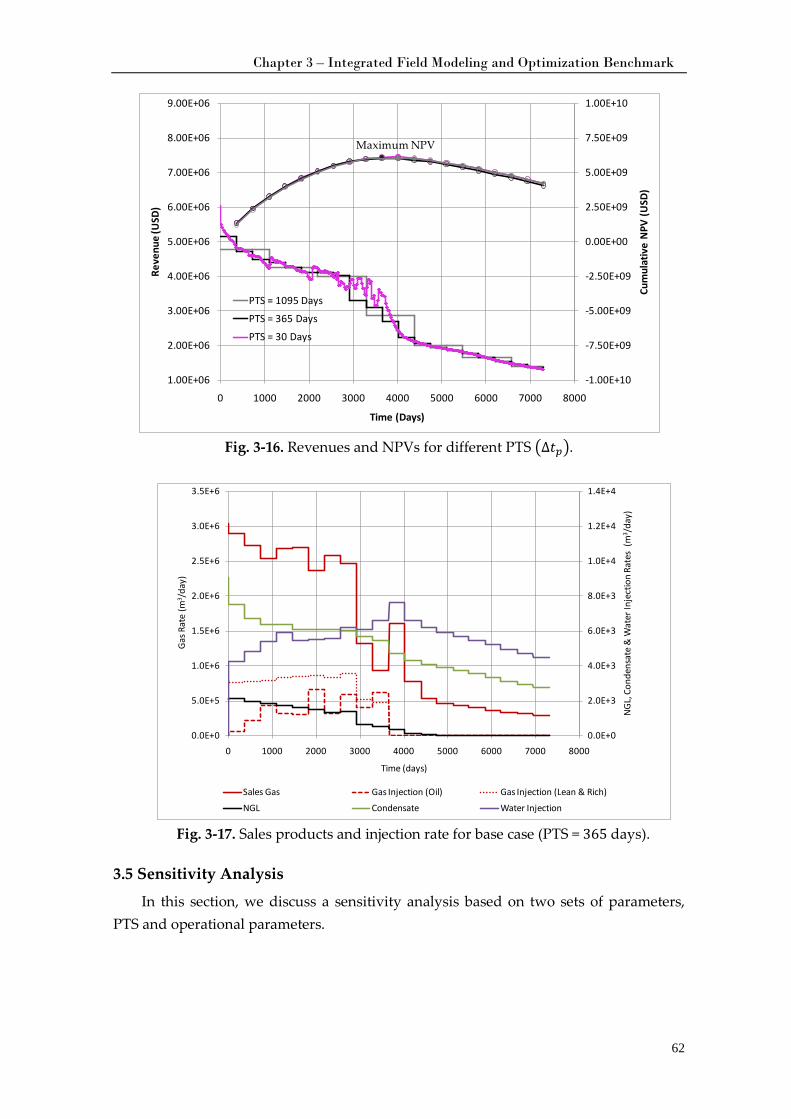
Chapter 3 – Integrated Field Modeling and Optimization Benchmark
62
Fig. 3-16. Revenues and NPVs for different PTS �∆𝑡𝑝�.
Fig. 3-17. Sales products and injection rate for base case (PTS = 365 days).
3.5 Sensitivity Analysis
In this section, we discuss a sensitivity analysis based on two sets of parameters, PTS and operational parameters.
-1.00E+10
-7.50E+09
-5.00E+09
-2.50E+09
0.00E+00
2.50E+09
5.00E+09
7.50E+09
1.00E+10
1.00E+06
2.00E+06
3.00E+06
4.00E+06
5.00E+06
6.00E+06
7.00E+06
8.00E+06
9.00E+06
0 1000 2000 3000 4000 5000 6000 7000 8000
Cum
ulat
ive
NPV
(USD
)
Reve
nue
(USD
)
Time (Days)
PTS = 1095 Days
PTS = 365 Days
PTS = 30 Days
Maximum NPV
0.0E+0
2.0E+3
4.0E+3
6.0E+3
8.0E+3
1.0E+4
1.2E+4
1.4E+4
0.0E+0
5.0E+5
1.0E+6
1.5E+6
2.0E+6
2.5E+6
3.0E+6
3.5E+6
0 1000 2000 3000 4000 5000 6000 7000 8000
NG
L, C
onde
nsat
e &
Wat
er In
ject
ion
Rate
s (m
3 /da
y)
Gas
Rat
e (m
3 /da
y)
Time (days)
Sales Gas Gas Injection (Oil) Gas Injection (Lean & Rich)
NGL Condensate Water Injection
Chapter 3 – Integrated Field Modeling and Optimization Benchmark
63
3.5.1. Sensitivity Analysis for Project Time Step
Fig. 3-16 shows that the selection of PTS influences revenue performance. Hence, silo-model dynamics deserves further investigation. The study of the silo-models is an interesting topic in investigating the dynamic behavior of the system. Here, we used four items to characterize silo-model performance:
• Comparison of reservoir output • Comparison of surface input • Comparison of surface output simulations • Comparison of injection composition and rates
Comparison of reservoir outputs. Fig. 3-18 shows the average value from each reservoir output for different PTS as an input for the surface process simulation. The comparison of reservoir outputs is made on the basis of the mole fraction of 𝐶3+ divided by 𝐶2− (𝐶3+/𝐶2−) excluding the 𝐻2𝑂, 𝐶𝑂2 and 𝑁𝑁2 components. The component 𝐶3+ consists of the sum of components 𝐶3, 𝐶4−6, 𝐶7𝑃1, 𝐶7𝑃2 and 𝐶7𝑃3 from the gas-condensate reservoirs and 𝐶3, 𝐶6, 𝐶10, 𝐶15 and 𝐶20 from the oil reservoir. Component 𝐶2− consists of the sum of 𝐶1 and 𝐶2.
Fig. 3-18 illustrates that the oil reservoir produces heavier components (𝐶3+) than the two gas-condensate reservoirs. Here, the rich gas-condensate reservoir produces more (𝐶3+) than the lean gas-condensate reservoir. There are some reservoirs that stop producing before 20 years, especially among gas-condensate reservoirs. The problem is caused by the reservoir pressure being too low to lift the liquid to the surface. Using a PTS of 30 days clearly shows dynamic reservoir output behavior caused by the composition changes inside the reservoir due to production and injection.
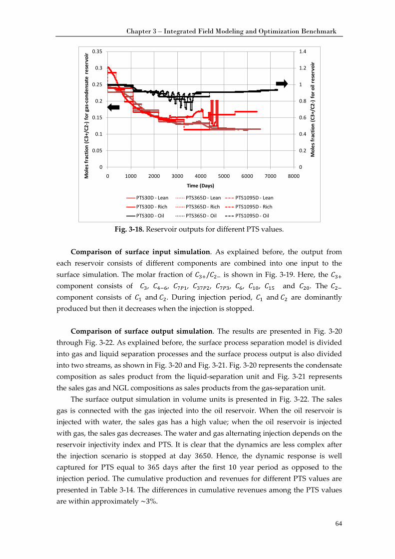
Chapter 3 – Integrated Field Modeling and Optimization Benchmark
64
Fig. 3-18. Reservoir outputs for different PTS values.
Comparison of surface input simulation. As explained before, the output from
each reservoir consists of different components are combined into one input to the surface simulation. The molar fraction of 𝐶3+/𝐶2− is shown in Fig. 3-19. Here, the 𝐶3+ component consists of 𝐶3, 𝐶4−6, 𝐶7𝑃1, 𝐶37𝑃2, 𝐶7𝑃3, 𝐶6, 𝐶10, 𝐶15 and 𝐶20. The 𝐶2− component consists of 𝐶1 and 𝐶2. During injection period, 𝐶1 and 𝐶2 are dominantly produced but then it decreases when the injection is stopped.
Comparison of surface output simulation. The results are presented in Fig. 3-20
through Fig. 3-22. As explained before, the surface process separation model is divided into gas and liquid separation processes and the surface process output is also divided into two streams, as shown in Fig. 3-20 and Fig. 3-21. Fig. 3-20 represents the condensate composition as sales product from the liquid-separation unit and Fig. 3-21 represents the sales gas and NGL compositions as sales products from the gas-separation unit.
The surface output simulation in volume units is presented in Fig. 3-22. The sales gas is connected with the gas injected into the oil reservoir. When the oil reservoir is injected with water, the sales gas has a high value; when the oil reservoir is injected with gas, the sales gas decreases. The water and gas alternating injection depends on the reservoir injectivity index and PTS. It is clear that the dynamics are less complex after the injection scenario is stopped at day 3650. Hence, the dynamic response is well captured for PTS equal to 365 days after the first 10 year period as opposed to the injection period. The cumulative production and revenues for different PTS values are presented in Table 3-14. The differences in cumulative revenues among the PTS values are within approximately ~3%.
0
0.2
0.4
0.6
0.8
1
1.2
1.4
0
0.05
0.1
0.15
0.2
0.25
0.3
0.35
0 1000 2000 3000 4000 5000 6000 7000 8000
Mol
es fr
actio
n (C
3+/C
2-) f
or o
il re
serv
oir
Mol
es fr
actio
n (C
3+/C
2-) f
or g
as-c
onde
nsat
e re
serv
oir
Time (Days)
PTS30D - Lean PTS365D - Lean PTS1095D - Lean
PTS30D - Rich PTS365D - Rich PTS1095D - Rich
PTS30D - Oil PTS365D - Oil PTS1095D - Oil
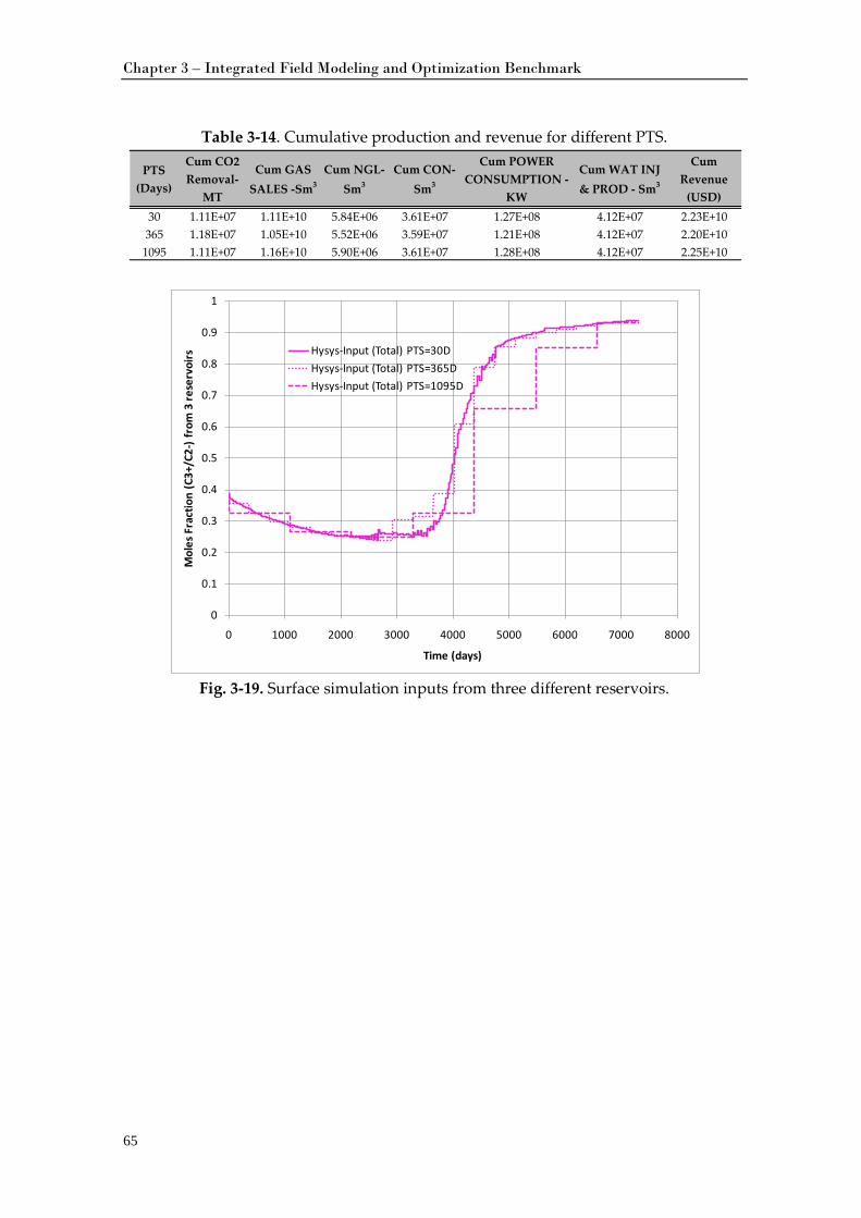
Chapter 3 – Integrated Field Modeling and Optimization Benchmark
65
Table 3-14. Cumulative production and revenue for different PTS.
Fig. 3-19. Surface simulation inputs from three different reservoirs.
PTS (Days)
Cum CO2 Removal-
MT
Cum GAS SALES -Sm3
Cum NGL-Sm3
Cum CON-Sm3
Cum POWER CONSUMPTION -
KW
Cum WAT INJ & PROD - Sm3
Cum Revenue
(USD)30 1.11E+07 1.11E+10 5.84E+06 3.61E+07 1.27E+08 4.12E+07 2.23E+10365 1.18E+07 1.05E+10 5.52E+06 3.59E+07 1.21E+08 4.12E+07 2.20E+101095 1.11E+07 1.16E+10 5.90E+06 3.61E+07 1.28E+08 4.12E+07 2.25E+10
0
0.1
0.2
0.3
0.4
0.5
0.6
0.7
0.8
0.9
1
0 1000 2000 3000 4000 5000 6000 7000 8000
Mol
es F
ract
ion
(C3+
/C2-
) fro
m 3
rese
rvoi
rs
Time (days)
Hysys-Input (Total) PTS=30DHysys-Input (Total) PTS=365DHysys-Input (Total) PTS=1095D
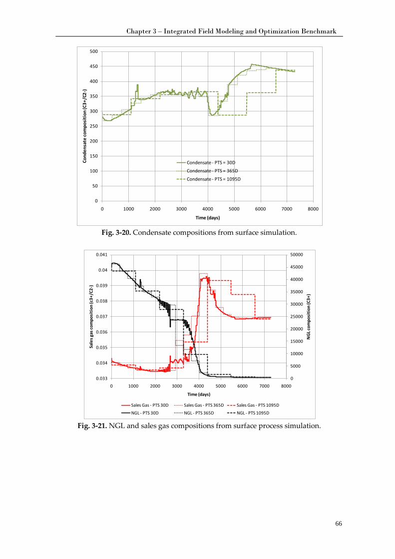
Chapter 3 – Integrated Field Modeling and Optimization Benchmark
66
Fig. 3-20. Condensate compositions from surface simulation.
Fig. 3-21. NGL and sales gas compositions from surface process simulation.
0
50
100
150
200
250
300
350
400
450
500
0 1000 2000 3000 4000 5000 6000 7000 8000
Cond
ensa
te co
mpo
siti
on (C
3+/C
2-)
Time (days)
Condensate - PTS = 30D
Condensate - PTS = 365D
Condensate - PTS = 1095D
0
5000
10000
15000
20000
25000
30000
35000
40000
45000
50000
0.033
0.034
0.035
0.036
0.037
0.038
0.039
0.04
0.041
0 1000 2000 3000 4000 5000 6000 7000 8000
NG
L com
posi
tion
(C3+
)
Sale
s gas
com
posi
tion
(c3+
/C2-
)
Time (days)
Sales Gas - PTS 30D Sales Gas - PTS 365D Sales Gas - PTS 1095D
NGL - PTS 30D NGL - PTS 365D NGL - PTS 1095D
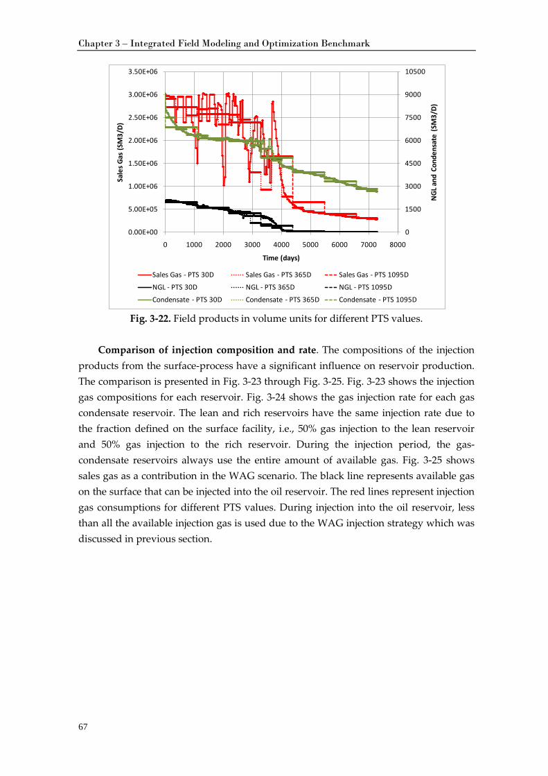
Chapter 3 – Integrated Field Modeling and Optimization Benchmark
67
Fig. 3-22. Field products in volume units for different PTS values.
Comparison of injection composition and rate. The compositions of the injection
products from the surface-process have a significant influence on reservoir production. The comparison is presented in Fig. 3-23 through Fig. 3-25. Fig. 3-23 shows the injection gas compositions for each reservoir. Fig. 3-24 shows the gas injection rate for each gas condensate reservoir. The lean and rich reservoirs have the same injection rate due to the fraction defined on the surface facility, i.e., 50% gas injection to the lean reservoir and 50% gas injection to the rich reservoir. During the injection period, the gas-condensate reservoirs always use the entire amount of available gas. Fig. 3-25 shows sales gas as a contribution in the WAG scenario. The black line represents available gas on the surface that can be injected into the oil reservoir. The red lines represent injection gas consumptions for different PTS values. During injection into the oil reservoir, less than all the available injection gas is used due to the WAG injection strategy which was discussed in previous section.
0
1500
3000
4500
6000
7500
9000
10500
0.00E+00
5.00E+05
1.00E+06
1.50E+06
2.00E+06
2.50E+06
3.00E+06
3.50E+06
0 1000 2000 3000 4000 5000 6000 7000 8000
NGL
and
Con
dens
ate
(SM
3/D)
Sale
s Gas
(SM
3/D)
Time (days)
Sales Gas - PTS 30D Sales Gas - PTS 365D Sales Gas - PTS 1095D
NGL - PTS 30D NGL - PTS 365D NGL - PTS 1095D
Condensate - PTS 30D Condensate - PTS 365D Condensate - PTS 1095D
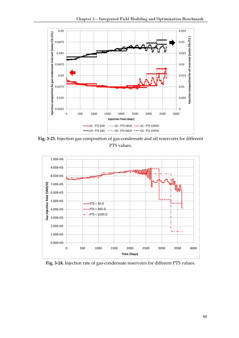
Chapter 3 – Integrated Field Modeling and Optimization Benchmark
68
Fig. 3-23. Injection gas composition of gas-condensate and oil reservoirs for different
PTS values.
Fig. 3-24. Injection rate of gas-condensate reservoirs for different PTS values.
0
0.005
0.01
0.015
0.02
0.025
0.03
0.035
0.0325
0.035
0.0375
0.04
0.0425
0.045
0.0475
0.05
0 500 1000 1500 2000 2500 3000 3500 4000
Inje
ctio
n co
mpo
sitio
n fo
r oil
rese
rvoi
r (m
oles
S3+
/C2-
)
Inje
ctio
n co
mpo
sitio
n fo
r gas
cond
ensa
te re
serv
oir (
mol
es C
3+/C
2-)
Injection Time (days)
GC - PTS 30D GC - PTS 365D GC - PTS 1095D
Oil - PTS 30D Oil - PTS 365D Oil - PTS 1095D
0.00E+00
1.00E+05
2.00E+05
3.00E+05
4.00E+05
5.00E+05
6.00E+05
7.00E+05
8.00E+05
9.00E+05
1.00E+06
0 500 1000 1500 2000 2500 3000 3500 4000
Gas I
njec
tion
Rate
(SM
3/D)
Time (Days)
PTS = 30 D
PTS = 365 D
PTS = 1095 D
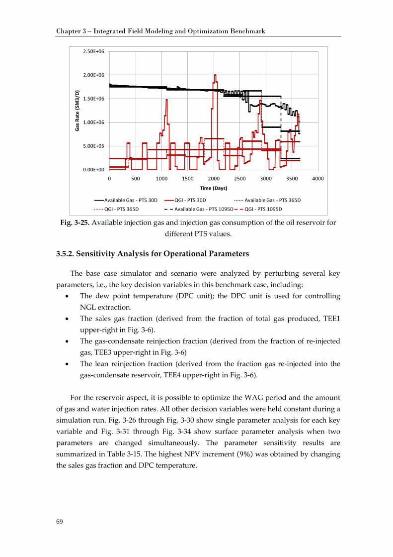
Chapter 3 – Integrated Field Modeling and Optimization Benchmark
69
Fig. 3-25. Available injection gas and injection gas consumption of the oil reservoir for
different PTS values.
3.5.2. Sensitivity Analysis for Operational Parameters
The base case simulator and scenario were analyzed by perturbing several key parameters, i.e., the key decision variables in this benchmark case, including:
• The dew point temperature (DPC unit); the DPC unit is used for controlling NGL extraction.
• The sales gas fraction (derived from the fraction of total gas produced, TEE1 upper-right in Fig. 3-6).
• The gas-condensate reinjection fraction (derived from the fraction of re-injected gas, TEE3 upper-right in Fig. 3-6)
• The lean reinjection fraction (derived from the fraction gas re-injected into the gas-condensate reservoir, TEE4 upper-right in Fig. 3-6).
For the reservoir aspect, it is possible to optimize the WAG period and the amount
of gas and water injection rates. All other decision variables were held constant during a simulation run. Fig. 3-26 through Fig. 3-30 show single parameter analysis for each key variable and Fig. 3-31 through Fig. 3-34 show surface parameter analysis when two parameters are changed simultaneously. The parameter sensitivity results are summarized in Table 3-15. The highest NPV increment (9%) was obtained by changing the sales gas fraction and DPC temperature.
0.00E+00
5.00E+05
1.00E+06
1.50E+06
2.00E+06
2.50E+06
0 500 1000 1500 2000 2500 3000 3500 4000
Gas R
ate
(SM
3/D)
Time (Days)
Available Gas - PTS 30D QGI - PTS 30D Available Gas - PTS 365D
QGI - PTS 365D Available Gas - PTS 1095D QGI - PTS 1095D
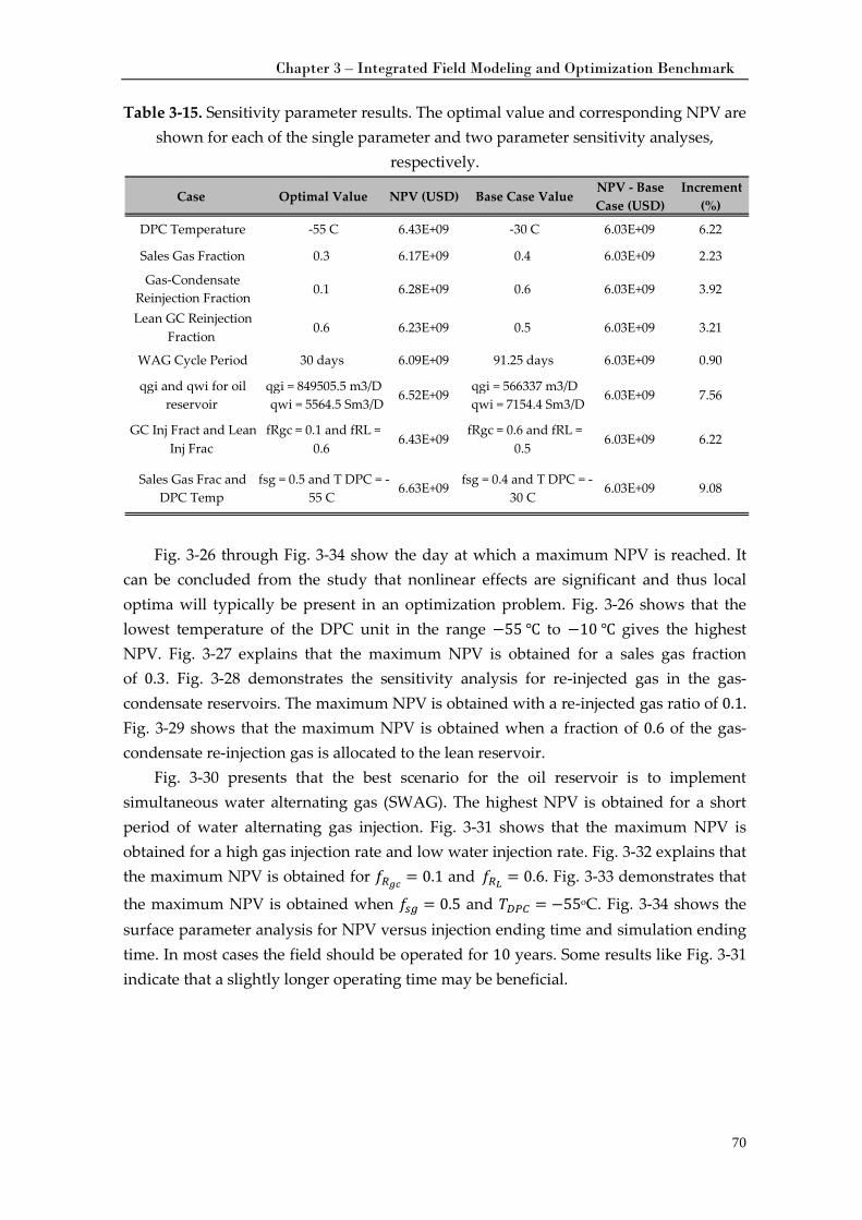
Chapter 3 – Integrated Field Modeling and Optimization Benchmark
70
Table 3-15. Sensitivity parameter results. The optimal value and corresponding NPV are shown for each of the single parameter and two parameter sensitivity analyses,
respectively.
Fig. 3-26 through Fig. 3-34 show the day at which a maximum NPV is reached. It can be concluded from the study that nonlinear effects are significant and thus local optima will typically be present in an optimization problem. Fig. 3-26 shows that the lowest temperature of the DPC unit in the range −55 ℃ to −10 ℃ gives the highest NPV. Fig. 3-27 explains that the maximum NPV is obtained for a sales gas fraction of 0.3. Fig. 3-28 demonstrates the sensitivity analysis for re-injected gas in the gas-condensate reservoirs. The maximum NPV is obtained with a re-injected gas ratio of 0.1. Fig. 3-29 shows that the maximum NPV is obtained when a fraction of 0.6 of the gas-condensate re-injection gas is allocated to the lean reservoir.
Fig. 3-30 presents that the best scenario for the oil reservoir is to implement simultaneous water alternating gas (SWAG). The highest NPV is obtained for a short period of water alternating gas injection. Fig. 3-31 shows that the maximum NPV is obtained for a high gas injection rate and low water injection rate. Fig. 3-32 explains that the maximum NPV is obtained for 𝑓𝑅𝑔𝑐 = 0.1 and 𝑓𝑅𝐿 = 0.6. Fig. 3-33 demonstrates that
the maximum NPV is obtained when 𝑓𝑠𝑔 = 0.5 and 𝑇𝑇𝐷𝑃𝐶 = −55oC. Fig. 3-34 shows the surface parameter analysis for NPV versus injection ending time and simulation ending time. In most cases the field should be operated for 10 years. Some results like Fig. 3-31 indicate that a slightly longer operating time may be beneficial.
Case Optimal Value NPV (USD) Base Case Value NPV - Base Case (USD)
Increment (%)
DPC Temperature -55 C 6.43E+09 -30 C 6.03E+09 6.22 Sales Gas Fraction 0.3 6.17E+09 0.4 6.03E+09 2.23 Gas-Condensate
Reinjection Fraction 0.1 6.28E+09 0.6 6.03E+09 3.92
Lean GC Reinjection Fraction 0.6 6.23E+09 0.5 6.03E+09 3.21
WAG Cycle Period 30 days 6.09E+09 91.25 days 6.03E+09 0.90 qgi and qwi for oil
reservoir qgi = 849505.5 m3/D qwi = 5564.5 Sm3/D 6.52E+09 qgi = 566337 m3/D
qwi = 7154.4 Sm3/D 6.03E+09 7.56
GC Inj Fract and Lean Inj Frac
fRgc = 0.1 and fRL = 0.6 6.43E+09 fRgc = 0.6 and fRL =
0.5 6.03E+09 6.22
Sales Gas Frac and DPC Temp
fsg = 0.5 and T DPC = - 55 C 6.63E+09 fsg = 0.4 and T DPC = -
30 C 6.03E+09 9.08
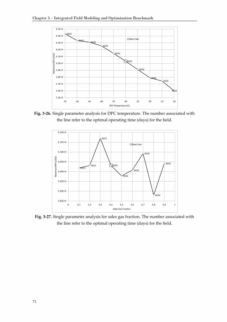
Chapter 3 – Integrated Field Modeling and Optimization Benchmark
71
Fig. 3-26. Single parameter analysis for DPC temperature. The number associated with
the line refer to the optimal operating time (days) for the field.
Fig. 3-27. Single parameter analysis for sales gas fraction. The number associated with
the line refer to the optimal operating time (days) for the field.
3650
36503650
3650
3650
3650
3650
36503650
3650
5.5E+9
5.6E+9
5.7E+9
5.8E+9
5.9E+9
6.0E+9
6.1E+9
6.2E+9
6.3E+9
6.4E+9
6.5E+9
-55 -50 -45 -40 -35 -30 -25 -20 -15 -10
Max
imum
NPV
(USD
)
DPC Temperature (C)
Base Case
40154015
4015
3650
3650
3650
3650
3650
3650
5.85E+9
5.90E+9
5.95E+9
6.00E+9
6.05E+9
6.10E+9
6.15E+9
6.20E+9
0 0.1 0.2 0.3 0.4 0.5 0.6 0.7 0.8 0.9 1
Max
imum
NPV
(USD
)
Sales Gas Fraction
Base Case
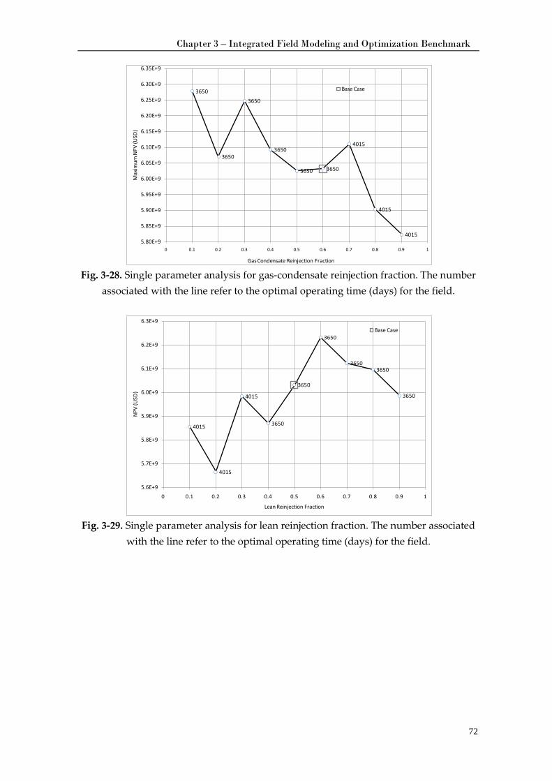
Chapter 3 – Integrated Field Modeling and Optimization Benchmark
72
Fig. 3-28. Single parameter analysis for gas-condensate reinjection fraction. The number
associated with the line refer to the optimal operating time (days) for the field.
Fig. 3-29. Single parameter analysis for lean reinjection fraction. The number associated
with the line refer to the optimal operating time (days) for the field.
3650
3650
3650
3650
3650 3650
4015
4015
40155.80E+9
5.85E+9
5.90E+9
5.95E+9
6.00E+9
6.05E+9
6.10E+9
6.15E+9
6.20E+9
6.25E+9
6.30E+9
6.35E+9
0 0.1 0.2 0.3 0.4 0.5 0.6 0.7 0.8 0.9 1
Max
imum
NPV
(USD
)
Gas Condensate Reinjection Fraction
Base Case
4015
4015
4015
3650
3650
3650
36503650
3650
5.6E+9
5.7E+9
5.8E+9
5.9E+9
6.0E+9
6.1E+9
6.2E+9
6.3E+9
0 0.1 0.2 0.3 0.4 0.5 0.6 0.7 0.8 0.9 1
NPV
(USD
)
Lean Reinjection Fraction
Base Case
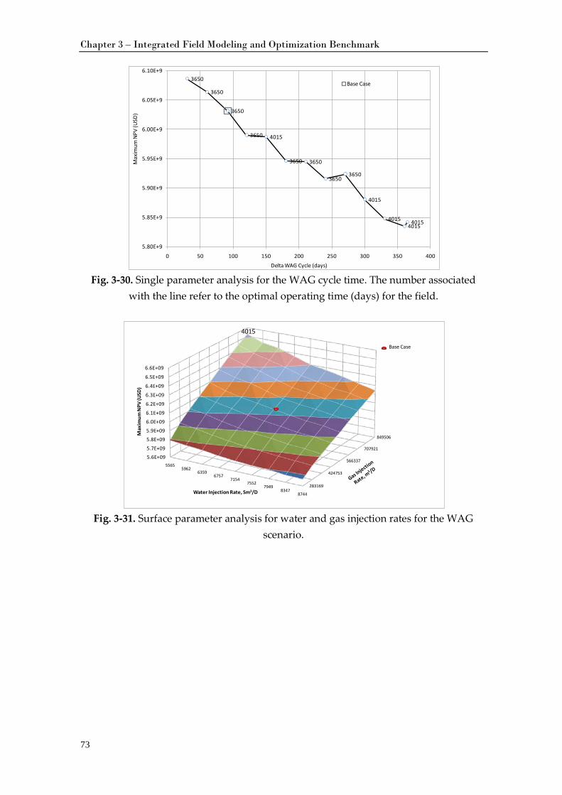
Chapter 3 – Integrated Field Modeling and Optimization Benchmark
73
Fig. 3-30. Single parameter analysis for the WAG cycle time. The number associated
with the line refer to the optimal operating time (days) for the field.
Fig. 3-31. Surface parameter analysis for water and gas injection rates for the WAG
scenario.
3650
3650
3650
3650 4015
3650 3650
36503650
4015
40154015
4015
5.80E+9
5.85E+9
5.90E+9
5.95E+9
6.00E+9
6.05E+9
6.10E+9
0 50 100 150 200 250 300 350 400
Max
imum
NPV
(USD
)
Delta WAG Cycle (days)
Base Case
283169
424753
566337
707921
849506
5.6E+095.7E+09
5.8E+09
5.9E+09
6.0E+09
6.1E+09
6.2E+09
6.3E+09
6.4E+09
6.5E+09
6.6E+09
55655962
63596757
71547552
79498347
8744
Max
imum
NPV
(USD
)
Water Injection Rate, Sm3/D
4015
Base Case
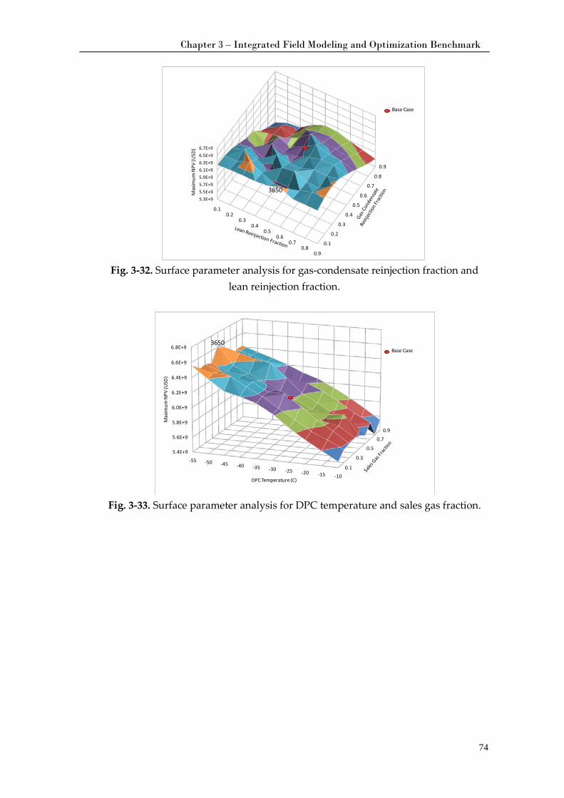
Chapter 3 – Integrated Field Modeling and Optimization Benchmark
74
Fig. 3-32. Surface parameter analysis for gas-condensate reinjection fraction and
lean reinjection fraction.
Fig. 3-33. Surface parameter analysis for DPC temperature and sales gas fraction.
0.1
0.2
0.3
0.4
0.5
0.6
0.7
0.8
0.9
5.3E+95.5E+95.7E+95.9E+96.1E+96.3E+96.5E+96.7E+9
0.10.2
0.30.4
0.50.6
0.70.8
0.9
Max
imum
NPV
(USD
)3650
Base Case
0.1
0.3
0.5
0.7
0.9
5.4E+9
5.6E+9
5.8E+9
6.0E+9
6.2E+9
6.4E+9
6.6E+9
6.8E+9
-55 -50 -45 -40 -35 -30 -25 -20 -15 -10
Max
imum
NPV
(USD
)
DPC Temperature (C)
3650Base Case
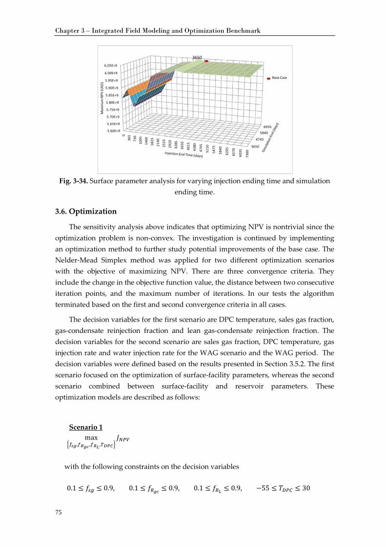
Chapter 3 – Integrated Field Modeling and Optimization Benchmark
75
Fig. 3-34. Surface parameter analysis for varying injection ending time and simulation
ending time.
3.6. Optimization
The sensitivity analysis above indicates that optimizing NPV is nontrivial since the optimization problem is non-convex. The investigation is continued by implementing an optimization method to further study potential improvements of the base case. The Nelder-Mead Simplex method was applied for two different optimization scenarios with the objective of maximizing NPV. There are three convergence criteria. They include the change in the objective function value, the distance between two consecutive iteration points, and the maximum number of iterations. In our tests the algorithm terminated based on the first and second convergence criteria in all cases.
The decision variables for the first scenario are DPC temperature, sales gas fraction, gas-condensate reinjection fraction and lean gas-condensate reinjection fraction. The decision variables for the second scenario are sales gas fraction, DPC temperature, gas injection rate and water injection rate for the WAG scenario and the WAG period. The decision variables were defined based on the results presented in Section 3.5.2. The first scenario focused on the optimization of surface-facility parameters, whereas the second scenario combined between surface-facility and reservoir parameters. These optimization models are described as follows:
max�𝑓𝑠𝑔,𝑓𝑅𝑔𝑐 ,𝑓𝑅𝐿 ,𝑇𝐷𝑃𝐶�
𝐽𝑁𝑃𝑉 Scenario 1
with the following constraints on the decision variables
0.1 ≤ 𝑓𝑠𝑔 ≤ 0.9, 0.1 ≤ 𝑓𝑅𝑔𝑐 ≤ 0.9, 0.1 ≤ 𝑓𝑅𝐿 ≤ 0.9, −55 ≤ 𝑇𝑇𝐷𝑃𝐶 ≤ 30
3650
4745
58406935
5.60E+9
5.65E+9
5.70E+9
5.75E+9
5.80E+9
5.85E+9
5.90E+9
5.95E+9
6.00E+9
6.05E+9
036
573
010
9514
6018
2521
9025
55
2920
3285
3650
4015
4380
4745
5110
5475
5840
6205
6570
6935
7300
Max
imum
NPV
(USD
)
3650
Base Case
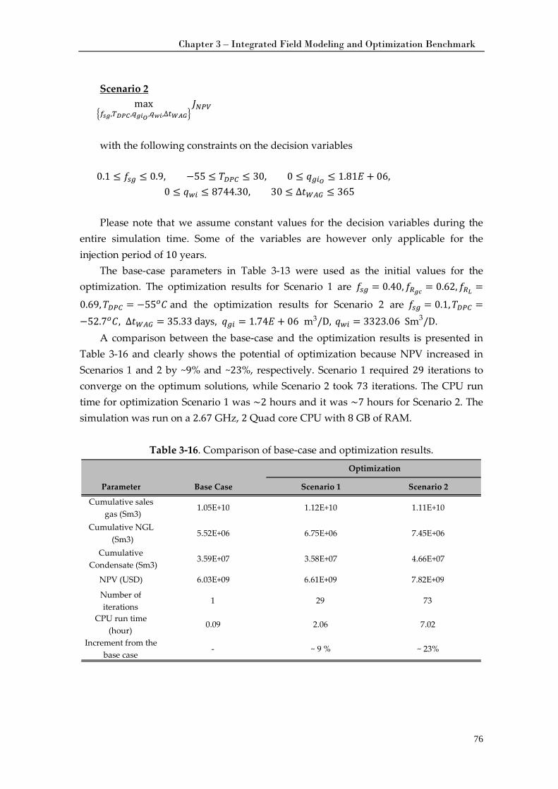
Chapter 3 – Integrated Field Modeling and Optimization Benchmark
76
max�𝑓𝑠𝑔,𝑇𝐷𝑃𝐶 ,𝑞𝑔𝑖𝑂 ,𝑞𝑤𝑖,∆𝑡𝑊𝐴𝐺�
𝐽𝑁𝑃𝑉 Scenario 2
with the following constraints on the decision variables
0.1 ≤ 𝑓𝑠𝑔 ≤ 0.9, −55 ≤ 𝑇𝑇𝐷𝑃𝐶 ≤ 30, 0 ≤ 𝑞𝑞𝑔𝑖𝑂 ≤ 1.81𝐸 + 06,0 ≤ 𝑞𝑞𝑤𝑖 ≤ 8744.30, 30 ≤ ∆𝑡𝑊𝐴𝐺 ≤ 365
Please note that we assume constant values for the decision variables during the
entire simulation time. Some of the variables are however only applicable for the injection period of 10 years.
The base-case parameters in Table 3-13 were used as the initial values for the optimization. The optimization results for Scenario 1 are 𝑓𝑠𝑔 = 0.40,𝑓𝑅𝑔𝑐 = 0.62,𝑓𝑅𝐿 =
0.69,𝑇𝑇𝐷𝑃𝐶 = −55𝑜𝐶 and the optimization results for Scenario 2 are 𝑓𝑠𝑔 = 0.1,𝑇𝑇𝐷𝑃𝐶 =−52.7𝑜𝐶, ∆𝑡𝑊𝐴𝐺 = 35.33 days, 𝑞𝑞𝑔𝑖 = 1.74𝐸 + 06 m3/D, 𝑞𝑞𝑤𝑖 = 3323.06 Sm3/D.
A comparison between the base-case and the optimization results is presented in Table 3-16 and clearly shows the potential of optimization because NPV increased in Scenarios 1 and 2 by ~9% and ~23%, respectively. Scenario 1 required 29 iterations to converge on the optimum solutions, while Scenario 2 took 73 iterations. The CPU run time for optimization Scenario 1 was ~2 hours and it was ~7 hours for Scenario 2. The simulation was run on a 2.67 GHz, 2 Quad core CPU with 8 GB of RAM.
Table 3-16. Comparison of base-case and optimization results.
Parameter Base Case Scenario 1 Scenario 2 Cumulative sales
gas (Sm3) 1.05E+10 1.12E+10 1.11E+10
Cumulative NGL (Sm3) 5.52E+06 6.75E+06 7.45E+06
Cumulative Condensate (Sm3) 3.59E+07 3.58E+07 4.66E+07
NPV (USD) 6.03E+09 6.61E+09 7.82E+09 Number of iterations 1 29 73
CPU run time (hour) 0.09 2.06 7.02
Increment from the base case - ~ 9 % ~ 23%
Optimization
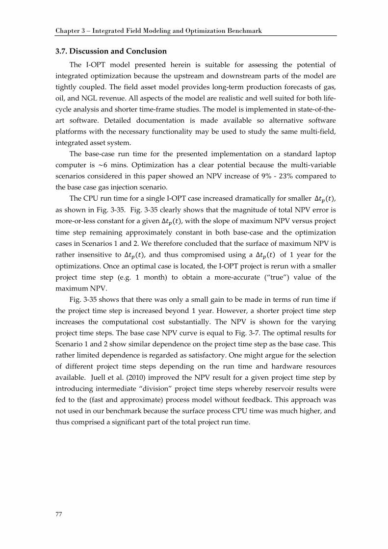
Chapter 3 – Integrated Field Modeling and Optimization Benchmark
77
3.7. Discussion and Conclusion
The I-OPT model presented herein is suitable for assessing the potential of integrated optimization because the upstream and downstream parts of the model are tightly coupled. The field asset model provides long-term production forecasts of gas, oil, and NGL revenue. All aspects of the model are realistic and well suited for both life-cycle analysis and shorter time-frame studies. The model is implemented in state-of-the-art software. Detailed documentation is made available so alternative software platforms with the necessary functionality may be used to study the same multi-field, integrated asset system.
The base-case run time for the presented implementation on a standard laptop computer is ~6 mins. Optimization has a clear potential because the multi-variable scenarios considered in this paper showed an NPV increase of 9% - 23% compared to the base case gas injection scenario.
The CPU run time for a single I-OPT case increased dramatically for smaller ∆𝑡𝑝(𝑡), as shown in Fig. 3-35. Fig. 3-35 clearly shows that the magnitude of total NPV error is more-or-less constant for a given ∆𝑡𝑝(𝑡), with the slope of maximum NPV versus project time step remaining approximately constant in both base-case and the optimization cases in Scenarios 1 and 2. We therefore concluded that the surface of maximum NPV is rather insensitive to ∆𝑡𝑝(𝑡), and thus compromised using a ∆𝑡𝑝(𝑡) of 1 year for the optimizations. Once an optimal case is located, the I-OPT project is rerun with a smaller project time step (e.g. 1 month) to obtain a more-accurate (“true”) value of the maximum NPV.
Fig. 3-35 shows that there was only a small gain to be made in terms of run time if the project time step is increased beyond 1 year. However, a shorter project time step increases the computational cost substantially. The NPV is shown for the varying project time steps. The base case NPV curve is equal to Fig. 3-7. The optimal results for Scenario 1 and 2 show similar dependence on the project time step as the base case. This rather limited dependence is regarded as satisfactory. One might argue for the selection of different project time steps depending on the run time and hardware resources available. Juell et al. (2010) improved the NPV result for a given project time step by introducing intermediate “division” project time steps whereby reservoir results were fed to the (fast and approximate) process model without feedback. This approach was not used in our benchmark because the surface process CPU time was much higher, and thus comprised a significant part of the total project run time.
Chapter 3 – Integrated Field Modeling and Optimization Benchmark
78
Fig. 3-35. CPU time and NPV for different project time steps.
4.0E+9
4.5E+9
5.0E+9
5.5E+9
6.0E+9
6.5E+9
7.0E+9
7.5E+9
8.0E+9
0
5
10
15
20
25
30
35
40
0 200 400 600 800 1000 1200 1400
Max
imum
NPV
(USD
)
CPU
tim
e (r
elat
ive
to th
e ba
se c
ase
time)
Project time step (days)
Scenario 2 Optimum
Scenario 1Optimum
Base Case
79
Chapter 4
A Mixed-Integer Non Linear Problem Formulation for Miscible WAG Injection
This chapter presents a mixed-integer problem formulation to evaluate optimal injection scenarios in an oil reservoir undergoing miscible water alternating gas (WAG) injection. The formulated injection scenarios consist of (i) gas injection (GI), (ii) water injection (WI), (iii) water alternating gas (WAG), and (iv) combination injection scenarios. Automated optimization of water-gas cyclic injection processes must allow for convergence to several operational solutions which are far removed from “traditional” short-cycle WAG scenario. Study cases are taken from a well-known single-well WAG problem, published in the SPE 5th comparative simulation study, Killough and Kossack (1987), Miscible WAG, and from a multi-well oil reservoir, the benchmark case described in Chapter 3 .
The economics of injection scenario are evaluated applying an optimization framework. The decision variables were tubing-head injection pressures for gas and water, gas and water injection volume targets, and the time when cyclic injection (WAG or WG) ends and is followed by WI, or GI, or depletion. A constrained Nelder-Mead Simplex method is used to optimize the aforementioned decision variables, wherein different initial values are tested to find an optimal solution. The field operating time may also be included as a decision variable. All injection scenarios were optimized for both natural-flow and artificial-lift production strategies. The study concluded that the artificial lift proposition was significantly better than natural-flow optimized strategies, since Net Present Value (NPV) increased by 8 − 31% on the particular system which was studied.
The proposed methodology is applicable to any oil reservoir where both surface water and gas injection is available. This work contributes to the literature by establishing a general mixed-integer problem formulation for water and gas injection and providing an efficient heuristic method for solving the problem. This section was written based on the paper Rahmawati et al. (2011).
4.1. Introduction
During the production lifetime of an oil field, reservoir production can potentially be divided into three distinct stages – (1) low cost depletion, (2) higher-cost enhanced oil recovery (EOR) with gas and/or water injection, and (3) a reduced-cost, end-life “tail”-production period. Two well control methods are used in oil production: natural flow
Chapter 4 – A MINLP Formulation for Miscible WAG Injection
80
and artificial lift. Natural flow is the simplest, least-expensive approach using individual-well choke control. Artificial lift consists of installing additional technology such as gas lift or pumps in a production well to enhance the rate of oil production by lowering the constraining bottomhole pressure (BHP).
After several years of production, an oil reservoir may not be able to maintain a sufficiently high economic production of oil due to a decrease in reservoir pressure, despite the fact that significant oil reserves remain in the reservoir. When this condition occurs, the reservoir typically enters the secondary recovery stage. Production may be improved by injecting gas and/or water to extract the remaining oil. At the end of secondary recovery, the oil production rate declines again, and a new production strategy may be introduced to increase recovery further.
The water alternating gas (WAG) injection technology was introduced by Caudle and Dyes (1958) in an effort to improve the macroscopic (areal and vertical) sweep efficiency by injecting water and microscopic pore-level sweep efficiency by injecting gas. WAG scenario have been studied extensively; Daoyong et al. (2000) applied optimization using Genetic Algorithms (GA) in China’s Pubei oil field. Kulkarni and Rao (2004) compared the WAG process to the gas injection (GI) process by conducting tertiary mode miscible and immiscible core-floods. The WAG mode of injection proved better than GI when “overall performance” was considered.
Gharbi (2004) tested WAG injection, Simultaneous Water Alternating Gas (SWAG) injection, and gas injection at the bottom of the reservoir with water injection at the top of the reservoir. The injectors use horizontal wells and the producers are vertical wells. The simulation results show that to simultaneously inject water at the reservoir top and gas at the reservoir bottom produced a better sweep efficiency and, therefore, the oil recovery was improved. Panda et al. (2009) optimized the Eileen West End Area in Greater Prudhoe Bay, operated by BP, using WAG. The key parameters evaluated were injection volume, injection rate, WAG ratios and WAG sequencing or WAG cycle number.
However, there are still significant areas in WAG optimization to be explored, such as the optimization of WAG by combining WAG with other injection scenario. Thus far, WAG has been implemented in several fields on the Norwegian Continental Shelf such as Snorre, Brae South, Statfjord, Brage, Gullfaks and Ekofisk; see also Christensen et al. (2001), Crogh et al. (2002), Awan et al. (2008), Talukdar and Instefjord (2008), Jensen et al. (2000), and Lien (1998).
Mathematical optimization has some merit in long term production optimization. In secondary recovery using water flooding injection, Nævdal et al. (2006), Van Essen et al. (2006), and Saputelli et al. (2009) have applied various optimization methods to improve oil recovery. A comprehensive overview is given in Jansen et al. (2008).
The goal for this research is to investigate injection scenarios for the purpose of optimizing oil production. A general mathematical formulation is introduced by assuming that surface water and injection gas are available. In this chapter, the problem
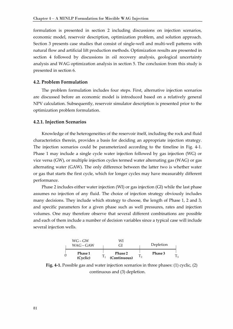
Chapter 4 – A MINLP Formulation for Miscible WAG Injection
81
formulation is presented in section 2 including discussions on injection scenarios, economic model, reservoir description, optimization problem, and solution approach. Section 3 presents case studies that consist of single-well and multi-well patterns with natural flow and artificial lift production methods. Optimization results are presented in section 4 followed by discussions in oil recovery analysis, geological uncertainty analysis and WAG optimization analysis in section 5. The conclusion from this study is presented in section 6.
4.2. Problem Formulation
The problem formulation includes four steps. First, alternative injection scenarios are discussed before an economic model is introduced based on a relatively general NPV calculation. Subsequently, reservoir simulator description is presented prior to the optimization problem formulation.
4.2.1. Injection Scenarios
Knowledge of the heterogeneities of the reservoir itself, including the rock and fluid characteristics therein, provides a basis for deciding an appropriate injection strategy. The injection scenarios could be parameterized according to the timeline in Fig. 4-1. Phase 1 may include a single cycle water injection followed by gas injection (WG) or vice versa (GW), or multiple injection cycles termed water alternating gas (WAG) or gas alternating water (GAW). The only difference between the latter two is whether water or gas that starts the first cycle, which for longer cycles may have measurably different performance.
Phase 2 includes either water injection (WI) or gas injection (GI) while the last phase assumes no injection of any fluid. The choice of injection strategy obviously includes many decisions. They include which strategy to choose, the length of Phase 1, 2 and 3, and specific parameters for a given phase such as well pressures, rates and injection volumes. One may therefore observe that several different combinations are possible and each of them include a number of decision variables since a typical case will include several injection wells.
Fig. 4-1. Possible gas and water injection scenarios in three phases: (1) cyclic, (2)
continuous and (3) depletion.
WG – GWWAG – GAW
WIGI Depletion
0 T1 T2 T3Phase 1(Cyclic)
Phase 2(Continuous)
Phase 3
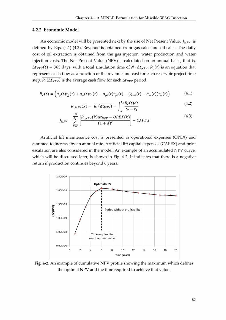
Chapter 4 – A MINLP Formulation for Miscible WAG Injection
82
4.2.2. Economic Model
An economic model will be presented next by the use of Net Present Value. 𝐽𝑁𝑃𝑉, is defined by Eqs. (4.1)-(4.3). Revenue is obtained from gas sales and oil sales. The daily cost of oil extraction is obtained from the gas injection, water production and water injection costs. The Net Present Value (NPV) is calculated on an annual basis, that is, ∆𝑡𝑁𝑃𝑉(𝑡) = 365 days, with a total simulation time of 𝑁𝑁 ∙ ∆𝑡𝑁𝑃𝑉. 𝑅𝑐(𝑡) is an equation that represents cash flow as a function of the revenue and cost for each reservoir project time step. 𝑅𝑐(∆𝑡𝑁𝑃𝑉)������������� is the average cash flow for each ∆𝑡𝑁𝑃𝑉 period.
𝑅𝑐(𝑡) = �𝑞𝑞𝑔(𝑡)𝑟𝑟𝑔(𝑡) + 𝑞𝑞𝑜(𝑡)𝑟𝑟𝑜(𝑡) − 𝑞𝑞𝑔𝑖(𝑡)𝑟𝑟𝑔𝑖(𝑡) − �𝑞𝑞𝑤𝑖(𝑡) + 𝑞𝑞𝑤(𝑡)�𝑟𝑟𝑤(𝑡)� (4.1)
𝑅𝑐𝑁𝑃𝑉(𝑘) = 𝑅𝑐(∆tNPV)������������� = �𝑅𝑐(𝑡)𝑑𝑑𝑡𝑡2 − 𝑡1
𝑡2
𝑡1 (4.2)
𝐽𝑁𝑃𝑉 = ��𝑅𝑐𝑁𝑃𝑉(𝑘)∆𝑡𝑁𝑃𝑉 − 𝑂𝑃𝑃𝐸𝑋(𝑘)
(1 + 𝑑𝑑)𝑘 � − 𝐶𝐴𝑃𝑃𝐸𝑋𝑁
𝑘=1
(4.3)
Artificial lift maintenance cost is presented as operational expenses (OPEX) and
assumed to increase by an annual rate. Artificial lift capital expenses (CAPEX) and price escalation are also considered in the model. An example of an accumulated NPV curve, which will be discussed later, is shown in Fig. 4-2. It indicates that there is a negative return if production continues beyond 6 years.
Fig. 4-2. An example of cumulative NPV profile showing the maximum which defines
the optimal NPV and the time required to achieve that value.
0.00E+00
5.00E+08
1.00E+09
1.50E+09
2.00E+09
2.50E+09
0 2 4 6 8 10 12 14 16 18 20
NPV
(USD
)
Time (Years)
Total NPVOptimal NPV
Period without profitability
Time required to reach optimal value
Chapter 4 – A MINLP Formulation for Miscible WAG Injection
83
4.2.3. Reservoir Description
A compositional reservoir simulator including well models will be used to provide information regarding the water injection rates (𝑞𝑞𝑤𝑖), gas injection rates �𝑞𝑞𝑔𝑖�, oil production rates (𝑞𝑞𝑜), water production rates (𝑞𝑞𝑤) and gas production rates �𝑞𝑞𝑔�. The compositional model consists of 𝑐 components (𝑁𝑁𝑐), which are divided into 𝑐 oil phase mole fractions (𝑥𝑐) and 𝑐 gas phase mole fractions (𝑦𝑐) at certain separator pressure and temperature conditions, �𝑃𝑃𝑠𝑒𝑝 and 𝑇𝑇𝑠𝑒𝑝�. In this study, the SENSOR® reservoir simulator is used for the reservoir model.
The water injection (𝑞𝑞𝑤𝑖) and gas injection �𝑞𝑞𝑔𝑖� rates are presented in a general form in Eq. (4.4) and Eq. (4.5), respectively. These rates are obtained as a function of reservoir properties and well model variables including tubing head pressure (THP) for water and gas injection (THP-WI and THP-GI), upper bound of water and gas injection rates �𝑞𝑞𝑔𝑖𝑚𝑎𝑥 and 𝑞𝑞𝑤𝑖𝑚𝑎𝑥�, and injection composition (𝑖𝑖𝑐). The differences lie in the pressure drop correlation. When gas is injected, gas flow tubing correlation is used to calculate the pressure drop, Fetkovich (1975). When water is injected, the Fetkovich equation is replaced by the Hagdorn-Brown correlation, Hagedorn and Brown (1965). A well tubing diameter (𝐷𝐷) for producer and injector is chosen and the THP table for water injection and production wells are generated using PROSPER software®.
Oil (𝑞𝑞𝑜), water (𝑞𝑞𝑤) and gas �𝑞𝑞𝑔� production rates are presented in Eq. (4.6), and they are a function of the reservoir properties, minimum BHP value �𝑃𝑃𝑤𝑓� or minimum THP value (𝑃𝑃𝑤ℎ) and liquid production rate target �𝑞𝑞𝑙𝑈�. The well model is included in the reservoir simulator only when production well is operated under natural flow method. The model integration is run in Pipe-It® software.
𝑞𝑞𝑤𝑖 = 𝑓�𝑠𝑠𝑤,𝐾𝑟𝑤 ,𝜇𝑤 ,𝐵𝑤 ,𝜌𝑙 ,𝜌𝑔,𝑃𝑃𝑟,𝑇𝑇𝐻𝑃𝑃 −𝑊𝐼, 𝑞𝑞𝑤𝑖𝑚𝑎𝑥,ℎ,ℎ𝑟,𝐷𝐷,𝐺𝑊𝑅, 𝑥𝑐 ,𝑦𝑐 , 𝑖𝑖𝑐� (4.4)
𝑞𝑞𝑔𝑖 = 𝑔𝑔�𝑠𝑠𝑔,𝐾𝑟𝑔, 𝜇𝑔 ,𝐵𝑔, 𝛾𝑔,𝑇𝑇� , �̅�,𝑃𝑃𝑟 ,𝑇𝑇𝐻𝑃𝑃 − 𝐺𝐼, 𝑞𝑞𝑔𝑖𝑚𝑎𝑥,ℎ,ℎ𝑟,𝐷𝐷,𝐺𝑊𝑅, 𝑥𝑐 ,𝑦𝑐 , 𝑖𝑖𝑐� (4.5)
𝑞𝑞𝑚
= ℎ �𝑠𝑠𝑔, 𝑠𝑠𝑜, 𝑠𝑠𝑤,𝐾𝑟𝑔,𝐾𝑟𝑜,𝐾𝑟𝑤 ,𝜇𝑔, 𝜇𝑜, 𝜇𝑤 ,𝐵𝑔,𝐵𝑤 ,𝐵𝑜,𝜌𝑜,𝜌𝑤 ,𝜌𝑔,𝑃𝑃𝑟,𝑃𝑃𝑤𝑓 ,
𝑃𝑃𝑤ℎ ,𝑞𝑞𝑙𝑈,ℎ,ℎ𝑟,𝐷𝐷,𝐺𝑂𝑅,𝑊𝐿𝐿𝑅, 𝑥𝑐 ,𝑦𝑐 , 𝑖𝑖𝑐 ,𝑇𝑇𝑠𝑒𝑝,𝑠𝑠𝑠𝑒𝑝 �
𝑚 = {𝑜𝑜,𝑤𝑤,𝑔𝑔}
(4.6)
4.2.4. Optimization Problem
The optimization problem is formulated next starting with the well specific variables and parameters.
𝑤𝑤𝑖 = �𝑤𝑤1𝑖 ,𝑤𝑤2𝑖 ,𝑤𝑤3𝑖 ,𝑤𝑤4𝑖�𝑇
𝑖𝑖 ∈ 𝐼 𝐼 = {1,2,⋯ ,𝑁𝑁𝑖}
Well specific continuous decision variables
𝑤𝑤1𝑖 gas injection volume (GIV) target constraint for phase 1 for injection well 𝑖𝑖, Mcf [m3].
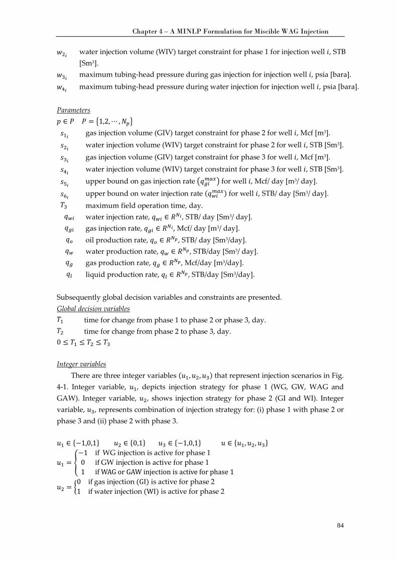
Chapter 4 – A MINLP Formulation for Miscible WAG Injection
84
𝑤𝑤2𝑖 water injection volume (WIV) target constraint for phase 1 for injection well 𝑖𝑖, STB [Sm3].
𝑤𝑤3𝑖 maximum tubing-head pressure during gas injection for injection well 𝑖𝑖, psia [bara].
𝑤𝑤4𝑖 maximum tubing-head pressure during water injection for injection well 𝑖𝑖, psia [bara].
𝑠𝑠 ∈ 𝑃𝑃 𝑃𝑃 = �1,2,⋯ ,𝑁𝑁𝑝� Parameters
𝑠𝑠1𝑖 gas injection volume (GIV) target constraint for phase 2 for well 𝑖𝑖, Mcf [m3].
𝑠𝑠2𝑖 water injection volume (WIV) target constraint for phase 2 for well 𝑖𝑖, STB [Sm3].
𝑠𝑠3𝑖 gas injection volume (GIV) target constraint for phase 3 for well 𝑖𝑖, Mcf [m3]. 𝑠𝑠4𝑖 water injection volume (WIV) target constraint for phase 3 for well 𝑖𝑖, STB [Sm3].
𝑠𝑠5𝑖 upper bound on gas injection rate �𝑞𝑞𝑔𝑖𝑚𝑎𝑥� for well 𝑖𝑖, Mcf/ day [m3/ day].
𝑠𝑠6𝑖 upper bound on water injection rate (𝑞𝑞𝑤𝑖𝑚𝑎𝑥) for well 𝑖𝑖, STB/ day [Sm3/ day]. 𝑇𝑇3 maximum field operation time, day. 𝑞𝑞𝑤𝑖 water injection rate, 𝑞𝑞𝑤𝑖 ∈ 𝑅𝑁𝑖, STB/ day [Sm3/ day]. 𝑞𝑞𝑔𝑖 gas injection rate, 𝑞𝑞𝑔𝑖 ∈ 𝑅𝑁𝑖, Mcf/ day [m3/ day]. 𝑞𝑞𝑜 oil production rate, 𝑞𝑞𝑜 ∈ 𝑅𝑁𝑝, STB/ day [Sm3/day]. 𝑞𝑞𝑤 water production rate, 𝑞𝑞𝑤 ∈ 𝑅𝑁𝑝, STB/day [Sm3/ day]. 𝑞𝑞𝑔 gas production rate, 𝑞𝑞𝑔 ∈ 𝑅𝑁𝑝, Mcf/day [m3/day]. 𝑞𝑞𝑙 liquid production rate, 𝑞𝑞𝑙 ∈ 𝑅𝑁𝑝, STB/day [Sm3/day].
Subsequently global decision variables and constraints are presented.
𝑇𝑇1 Global decision variables
time for change from phase 1 to phase 2 or phase 3, day. 𝑇𝑇2 time for change from phase 2 to phase 3, day. 0 ≤ 𝑇𝑇1 ≤ 𝑇𝑇2 ≤ 𝑇𝑇3
There are three integer variables (𝑢1,𝑢2,𝑢3) that represent injection scenarios in Integer variables
Fig. 4-1. Integer variable, 𝑢1, depicts injection strategy for phase 1 (WG, GW, WAG and GAW). Integer variable, 𝑢2, shows injection strategy for phase 2 (GI and WI). Integer variable, 𝑢3, represents combination of injection strategy for: (i) phase 1 with phase 2 or phase 3 and (ii) phase 2 with phase 3.
𝑢1 ∈ {−1,0,1} 𝑢2 ∈ {0,1} 𝑢3 ∈ {−1,0,1} 𝑢 ∈ {𝑢1,𝑢2,𝑢3}
𝑢1 = �−1 if WG injection is active for phase 10 if GW injection is active for phase 1 1 if WAG or GAW injection is active for phase 1
�
𝑢2 = �0 if gas injection (GI) is active for phase 2 1 if water injection (WI) is active for phase 2
�
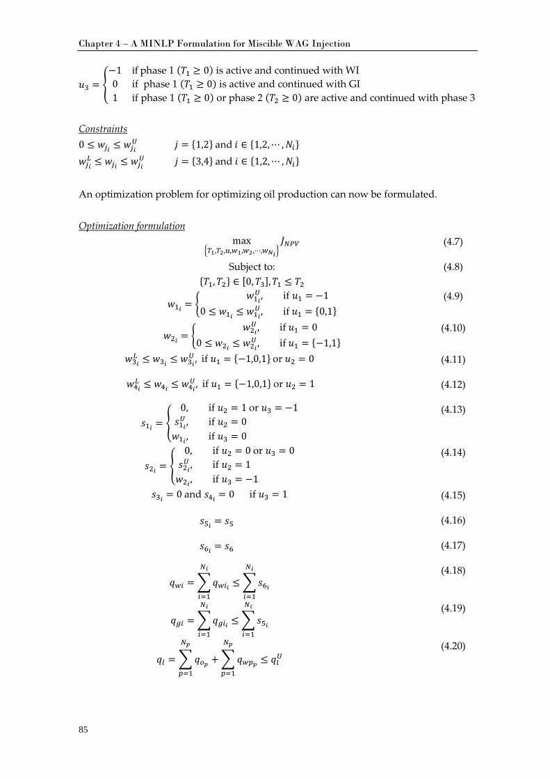
Chapter 4 – A MINLP Formulation for Miscible WAG Injection
85
𝑢3 = �−1 if phase 1 (𝑇𝑇1 ≥ 0) is active and continued with WI 0 if phase 1 (𝑇𝑇1 ≥ 0) is active and continued with GI1 if phase 1 (𝑇𝑇1 ≥ 0) or phase 2 (𝑇𝑇2 ≥ 0) are active and continued with phase 3
�
0 ≤ 𝑤𝑤𝑗𝑖 ≤ 𝑤𝑤𝑗𝑖𝑈 𝑗 = {1,2} and 𝑖𝑖 ∈ {1,2,⋯ ,𝑁𝑁𝑖}
Constraints
𝑤𝑤𝑗𝑖𝐿 ≤ 𝑤𝑤𝑗𝑖 ≤ 𝑤𝑤𝑗𝑖
𝑈 𝑗 = {3,4} and 𝑖𝑖 ∈ {1,2,⋯ ,𝑁𝑁𝑖} An optimization problem for optimizing oil production can now be formulated.
max�𝑇1,𝑇2,𝑢,𝑤1,𝑤2,⋯,𝑤𝑁𝑖�
𝐽𝑁𝑃𝑉 Optimization formulation
(4.7)
Subject to: {𝑇𝑇1,𝑇𝑇2} ∈ [0,𝑇𝑇3],𝑇𝑇1 ≤ 𝑇𝑇2
(4.8)
𝑤𝑤1𝑖 = �𝑤𝑤1𝑖𝑈 , if 𝑢1 = −1
0 ≤ 𝑤𝑤1𝑖 ≤ 𝑤𝑤1𝑖𝑈 , if 𝑢1 = {0,1}
� (4.9)
𝑤𝑤2𝑖 = �𝑤𝑤2𝑖𝑈 , if 𝑢1 = 0
0 ≤ 𝑤𝑤2𝑖 ≤ 𝑤𝑤2𝑖𝑈 , if 𝑢1 = {−1,1}
� (4.10)
𝑤𝑤3𝑖𝐿 ≤ 𝑤𝑤3𝑖 ≤ 𝑤𝑤3𝑖
𝑈 , if 𝑢1 = {−1,0,1} or 𝑢2 = 0 (4.11)
𝑤𝑤4𝑖𝐿 ≤ 𝑤𝑤4𝑖 ≤ 𝑤𝑤4𝑖
𝑈, if 𝑢1 = {−1,0,1} or 𝑢2 = 1 (4.12)
𝑠𝑠1𝑖 = �0, if 𝑢2 = 1 or 𝑢3 = −1𝑠𝑠1𝑖𝑈 , if 𝑢2 = 0
𝑤𝑤1𝑖 , if 𝑢3 = 0�
(4.13)
𝑠𝑠2𝑖 = �0, if 𝑢2 = 0 or 𝑢3 = 0𝑠𝑠2𝑖𝑈 , if 𝑢2 = 1
𝑤𝑤2𝑖 , if 𝑢3 = −1�
(4.14)
𝑠𝑠3𝑖 = 0 and 𝑠𝑠4𝑖 = 0 if 𝑢3 = 1 (4.15)
𝑠𝑠5𝑖 = 𝑠𝑠5 (4.16)
𝑠𝑠6𝑖 = 𝑠𝑠6 (4.17)
𝑞𝑞𝑤𝑖 = �𝑞𝑞𝑤𝑖𝑖
𝑁𝑖
𝑖=1
≤�𝑠𝑠6𝑖
𝑁𝑖
𝑖=1
(4.18)
𝑞𝑞𝑔𝑖 = �𝑞𝑞𝑔𝑖𝑖
𝑁𝑖
𝑖=1
≤�𝑠𝑠5𝑖
𝑁𝑖
𝑖=1
(4.19)
𝑞𝑞𝑙 = �𝑞𝑞𝑜𝑝
𝑁𝑝
𝑝=1
+ �𝑞𝑞𝑤𝑝𝑝
𝑁𝑝
𝑝=1
≤ 𝑞𝑞𝑙𝑈 (4.20)
Chapter 4 – A MINLP Formulation for Miscible WAG Injection
86
𝑞𝑞𝑔 = �𝑞𝑞𝑔𝑝
𝑁𝑝
𝑝=1
≤ 𝑞𝑞𝑔𝑈 (4.21)
Eqs. (4.4)-(4.6)
4.2.5. Solution Approach
The optimization problem presented in the previous subsection is a mixed integer nonlinear problem (MINLP). Several researchers have conducted research on various MINLP problems. Kosmidis et al. (2005) discussed well scheduling problem and solved MINLP problem following an outer approximation (OA) type of algorithm. Camponogara and Plucenio (2008) developed a column generation formulation that renders a compressor scheduling problem as a MINLP problem. Rashid et al. (2011) treated choke control on gas-lift well optimization as a MINLP and the Bonmin solver was utilized for this purpose. The MINLP optimization problem is challenging to solve and a heuristic approach is chosen in this case by trying for each integer value and/or combination to solve the problem so as to find the highest NPV and the best injection strategy. The approach is presented in Fig. 4-3. The procedure consists of four steps.
The first step (continuous injection strategy) consists of performing a case matrix (CM) for water injection and gas injection scenarios independently. The tubing head pressure for water injection (𝑤𝑤4) is gridded between a lower and an upper value, and NPV is calculated for each of these values. The same procedure is run for gas injection. The pressures which gave the maximum values in the two cases are used for the second step. The second step (cyclic injection strategy), a CM method is again used to find the injection volume ranges for the WG and GW scenarios. The Nelder-Mead Simplex method is used for optimization in the second and third steps by performing the simulation using different initial values. There are two types of optimization for steps 2 and 3 using different decision variables:
• The optimization of single-cycle WG and GW injection scenarios using decision variables that include THP (𝑤𝑤3 and 𝑤𝑤4), and GIV target (𝑤𝑤1) for GW injection or THP (𝑤𝑤3 and 𝑤𝑤4), and WIV target (𝑤𝑤2) for the WG strategy.
• The optimization of multi-cycle WAG and GAW injection scenarios using THP (𝑤𝑤3 and 𝑤𝑤4), GIV target (𝑤𝑤1), and WIV target (𝑤𝑤2) as decision variables for both injection scenarios.
Fig. 4-3 is applicable either for single-well or multi-well cases. Single-well injection optimization strategy uses the diagram inside the thick line, while the multi-well optimization case uses the whole diagram. However, when performing optimization for the multi-well case, the problem formulation includes optimization for wells under the same operating conditions (diagram inside thick line) and optimization for wells under different operating conditions (diagram inside dash line). Optimization for the multi-
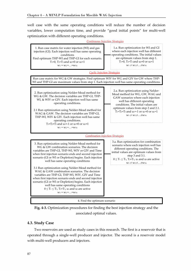
Chapter 4 – A MINLP Formulation for Miscible WAG Injection
87
well case with the same operating conditions will reduce the number of decision variables, lower computation time, and provide “good initial points” for multi-well optimization with different operating conditions.
Fig. 4-3. Optimization procedures for finding the best injection strategy and the
associated optimal values.
4.3. Study Case
Two reservoirs are used as study cases in this research. The first is a reservoir that is operated through a single-well producer and injector. The second is a reservoir model with multi-well producers and injectors.
1. Run case matrix for water injection (WI) and gas injection (GI). Each injection well has same operating
conditionsFind optimum THP-WI and THP-GI for each scenario.
T1=0, T2=T3 and u2=0 or u2=1w1 = w2 =…=wNi
1.a. Run optimization for WI and GI where each injection well has different operating conditions. The initial values
are optimum values from step 1. T1=0, T2=T3 and u2=0 or u2=1
w1 ≠ w2 ≠…≠wNi
Run case matrix for WG & GW strategies. Find optimum WIV for WG and GIV for GW where THP-WI and THP-GI are maximum values from step 1. Each injection well has same operating conditions.
2. Run optimization using Nelder-Mead method for WG & GW. The decision variables are THP-GI, THP-
WI, & WIV or GIV. Each injection well has same operating conditions.
2.1 Run optimization using Nelder-Mead method for WAG & GAW. The decision variables are THP-GI, THP-WI, WIV & GIV. Each injection well has same
operating conditions.T1=T2=T3 and u1=-1 or u1=0 or u1=1
w1 = w2 =…=wNi
2.a. Run optimization using Nelder-Mead method for WG, GW, WAG and GAW scenarios where each injection
well has different operating conditions. The initial values are
optimum values from step 2 and 2.1.T1=T2=T3 and u1=-1 or u1=0 or u1=1
w1 ≠ w2 ≠…≠wNi
3. Run optimization using Nelder-Mead method for WG & GW combination scenarios. The decision
variables are THP-GI, THP-WI, WIV or GIV and Time when first injection scenario ends and second injection scenario (GI or WI or Depletion) begins. Each injection
well has same operating conditions
3.1 Run optimization using Nelder-Mead method for WAG & GAW combination scenarios. The decision variables are THP-GI, THP-WI, WIV, GIV and Time
when first injection scenario ends and second injection scenario (GI or WI or Depletion) begins. Each injection
well has same operating conditions 0 ≤ T1 ≤ T3, T2=T3, u1 and u3 are active
w1 = w2 =…=wNi
4. Find the optimum scenario
3.a. Run optimization for combination scenario where each injection well has
different operating conditions. The initial values are optimum values from
step 3 and 3.1.0 ≤ T1 ≤ T3, T2=T3, u1 and u3 are active
w1 ≠ w2 ≠…≠wNi
Continuous Injection Strategies
Cyclic Injection Strategies
Combination Injection Strategies
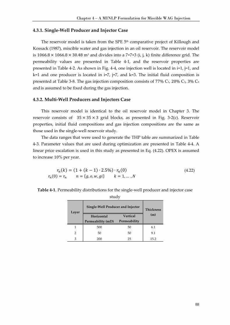
Chapter 4 – A MINLP Formulation for Miscible WAG Injection
88
4.3.1. Single-Well Producer and Injector Case
The reservoir model is taken from the SPE 5th comparative project of Killough and Kossack (1987), miscible water and gas injection in an oil reservoir. The reservoir model is 1066.8 × 1066.8 × 30.48 m3 and divides into a 7×7×3 (i, j, k) finite difference grid. The permeability values are presented in Table 4-1, and the reservoir properties are presented in Table 4-2. As shown in Fig. 4-4, one injection well is located in i=1, j=1, and k=1 and one producer is located in i=7, j=7, and k=3. The initial fluid composition is presented at Table 3-8. The gas injection composition consists of 77% C1, 20% C3, 3% C6
and is assumed to be fixed during the gas injection.
4.3.2. Multi-Well Producers and Injectors Case
This reservoir model is identical to the oil reservoir model in Chapter 3. The reservoir consists of 35 × 35 × 3 grid blocks, as presented in Fig. 3-2(c). Reservoir properties, initial fluid compositions and gas injection compositions are the same as those used in the single-well reservoir study.
The data ranges that were used to generate the THP table are summarized in Table 4-3. Parameter values that are used during optimization are presented in Table 4-4. A linear price escalation is used in this study as presented in Eq. (4.22). OPEX is assumed to increase 10% per year.
𝑟𝑟𝑛(𝑘) = (1 + (𝑘 − 1) ∙ 2.5%) ∙ 𝑟𝑟𝑛(0)
𝑟𝑟𝑛(0) = 𝑟𝑟𝑛 𝑛 = {𝑔𝑔, 𝑜𝑜,𝑤𝑤,𝑔𝑔𝑖𝑖} 𝑘 = 1, … ,𝑁𝑁 (4.22)
Table 4-1. Permeability distributions for the single-well producer and injector case
study
Horizontal Permeability (mD)
Vertical Permeability
1 500 50 6.1
2 50 50 9.1
3 200 25 15.2
Single-Well Producer and InjectorThickness
(m)Layer
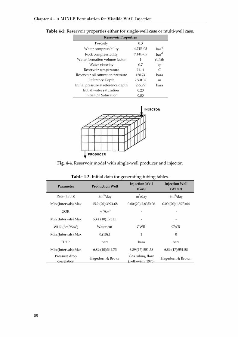
Chapter 4 – A MINLP Formulation for Miscible WAG Injection
89
Table 4-2. Reservoir properties either for single-well case or multi-well case.
Fig. 4-4. Reservoir model with single-well producer and injector.
Table 4-3. Initial data for generating tubing tables.
0.34.71E-05 bar-1
7.14E-05 bar-1
1 rb/stb0.7 cp
71.11 C158.74 bara
2560.32 m275.79 bara0.200.80
Reference DepthInitial pressure @ reference depth
Initial water saturation Initial Oil Saturation
Reservoir Properties
Rock compressibility
PorosityWater compressibility
Water formation volume factorWater viscosity
Reservoir temperatureReservoir oil saturation pressure
Rate (Units) Sm3/day m3/day Sm3/day
Min:(Intervals):Max 15.9:(20):3974.68 0.00:(20):2.83E+06 0.00:(20):1.59E+04
GOR m3/Sm3 - -
Min:(Intervals):Max 53.4:(10):1781.1 - -
WLR (Sm3/Sm3) Water cut GWR GWR
Min:(Intervals):Max 0:(10):1 1 0
THP bara bara bara
Min:(Intervals):Max 6.89:(10):344.73 6.89:(17):551.58 6.89:(17):551.58
Pressure drop correlation
Hagedorn & Brown Gas tubing flow (Fetkovich, 1975)
Hagedorn & Brown
Parameter Production WellInjection Well
(Gas)Injection Well
(Water)
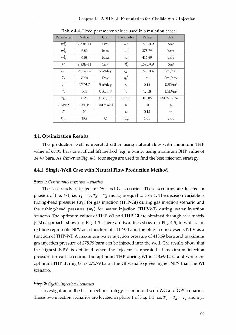
Chapter 4 – A MINLP Formulation for Miscible WAG Injection
90
Table 4-4. Fixed parameter values used in simulation cases.
4.4. Optimization Results
The production well is operated either using natural flow with minimum THP value of 68.95 bara or artificial lift method, e.g. a pump, using minimum BHP value of 34.47 bara. As shown in Fig. 4-3, four steps are used to find the best injection strategy.
4.4.1. Single-Well Case with Natural Flow Production Method
Step 1: Continuous injection scenariosThe case study is tested for WI and GI scenarios. These scenarios are located in
phase 2 of
Fig. 4-1, i.e. 𝑇𝑇1 = 0, 𝑇𝑇2 = 𝑇𝑇3 and 𝑢2 is equal to 0 or 1. The decision variable is tubing-head pressure (𝑤𝑤3) for gas injection (THP-GI) during gas injection scenario and the tubing-head pressure (𝑤𝑤4) for water injection (THP-WI) during water injection scenario. The optimum values of THP-WI and THP-GI are obtained through case matrix (CM) approach, shown in Fig. 4-5. There are two lines shown in Fig. 4-5, in which, the red line represents NPV as a function of THP-GI and the blue line represents NPV as a function of THP-WI. A maximum water injection pressure of 413.69 bara and maximum gas injection pressure of 275.79 bara can be injected into the well. CM results show that the highest NPV is obtained when the injector is operated at maximum injection pressure for each scenario. The optimum THP during WI is 413.69 bara and while the optimum THP during GI is 275.79 bara. The GI scenario gives higher NPV than the WI scenario.
Step 2: Cyclic Injection Scenarios
Investigation of the best injection strategy is continued with WG and GW scenarios. These two injection scenarios are located in phase 1 of
Fig. 4-1, i.e. 𝑇𝑇1 = 𝑇𝑇2 = 𝑇𝑇3 and 𝑢1is
Parameter Value Unit Parameter Value Unit
𝑤𝑤1𝑖𝑖𝑈𝑈 2.83E+11 Sm3 𝑤𝑤2𝑖𝑖
𝑈𝑈 1.59E+09 Sm3
𝑤𝑤3𝑖𝑖𝐿𝐿 6.89 bara 𝑤𝑤3𝑖𝑖
𝑈𝑈 275.79 bara
𝑤𝑤4𝑖𝑖𝐿𝐿 6.89 bara 𝑤𝑤4𝑖𝑖
𝑈𝑈 413.69 bara
𝑠𝑠1𝑖𝑖𝑈𝑈 2.83E+11 Sm3 𝑠𝑠2𝑖𝑖
𝑈𝑈 1.59E+09 Sm3
𝑠𝑠5 2.83e+06 Sm3/day 𝑠𝑠6 1.59E+04 Sm3/day
𝑇𝑇3 7300 Day 𝑞𝑞𝑔𝑔𝑈𝑈 ∞ Sm3/day
𝑞𝑞𝑙𝑙𝑈𝑈 3974.7 Sm3/day 𝑟𝑟𝑔𝑔 0.18 USD/m3
𝑟𝑟𝑜𝑜 503 USD/m3 𝑟𝑟𝑤𝑤 12.58 USD/m3
𝑟𝑟𝑔𝑔𝑖𝑖 0.25 USD/m3 OPEX 1E+06 USD/year/well
CAPEX 3E+06 USD/ well
𝑑𝑑 10 %
𝑁𝑁 20 𝐷𝐷 0.13 m
𝑇𝑇𝑠𝑠𝑠𝑠𝑠𝑠 15.6 C 𝑃𝑃𝑠𝑠𝑠𝑠𝑠𝑠 1.01 bara
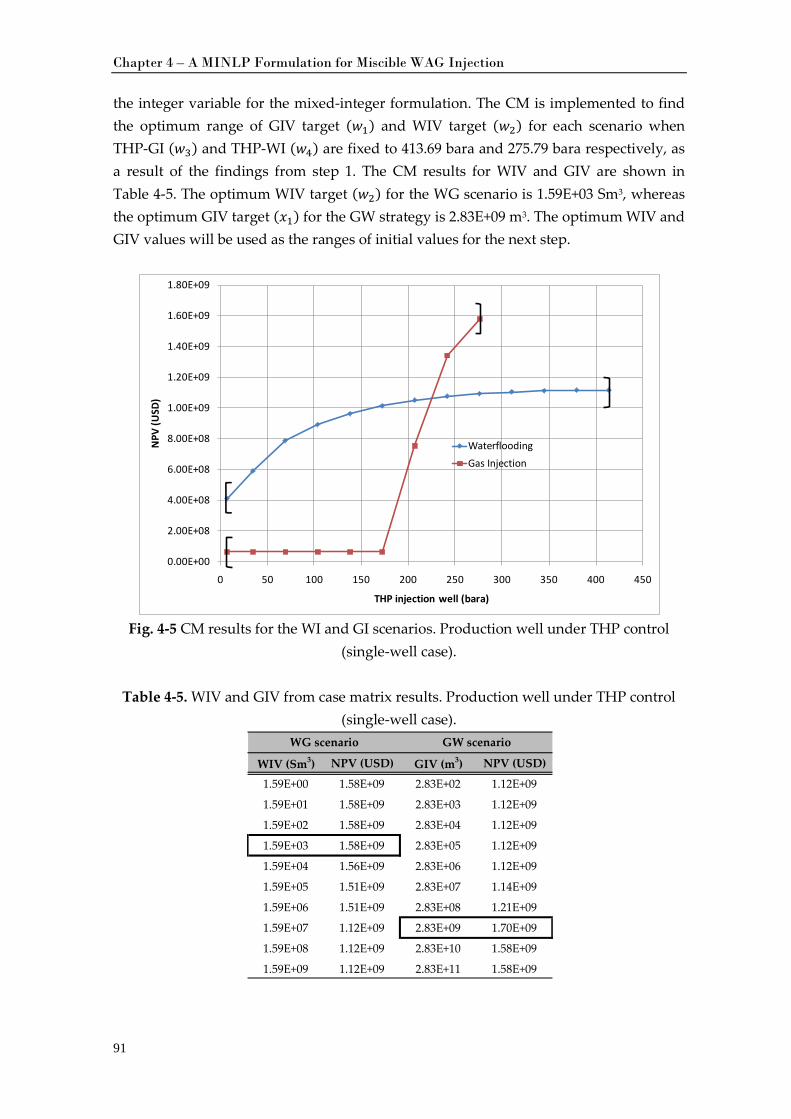
Chapter 4 – A MINLP Formulation for Miscible WAG Injection
91
the integer variable for the mixed-integer formulation. The CM is implemented to find the optimum range of GIV target (𝑤𝑤1) and WIV target (𝑤𝑤2) for each scenario when THP-GI (𝑤𝑤3) and THP-WI (𝑤𝑤4) are fixed to 413.69 bara and 275.79 bara respectively, as a result of the findings from step 1. The CM results for WIV and GIV are shown in Table 4-5. The optimum WIV target (𝑤𝑤2) for the WG scenario is 1.59E+03 Sm3, whereas the optimum GIV target (𝑥1) for the GW strategy is 2.83E+09 m3. The optimum WIV and GIV values will be used as the ranges of initial values for the next step.
Fig. 4-5 CM results for the WI and GI scenarios. Production well under THP control
(single-well case).
Table 4-5. WIV and GIV from case matrix results. Production well under THP control (single-well case).
0.00E+00
2.00E+08
4.00E+08
6.00E+08
8.00E+08
1.00E+09
1.20E+09
1.40E+09
1.60E+09
1.80E+09
0 50 100 150 200 250 300 350 400 450
NPV
(USD
)
THP injection well (bara)
WaterfloodingGas Injection
WIV (Sm3) NPV (USD) GIV (m3) NPV (USD)
1.59E+00 1.58E+09 2.83E+02 1.12E+09
1.59E+01 1.58E+09 2.83E+03 1.12E+09
1.59E+02 1.58E+09 2.83E+04 1.12E+09
1.59E+03 1.58E+09 2.83E+05 1.12E+09
1.59E+04 1.56E+09 2.83E+06 1.12E+09
1.59E+05 1.51E+09 2.83E+07 1.14E+09
1.59E+06 1.51E+09 2.83E+08 1.21E+09
1.59E+07 1.12E+09 2.83E+09 1.70E+09
1.59E+08 1.12E+09 2.83E+10 1.58E+09
1.59E+09 1.12E+09 2.83E+11 1.58E+09
WG scenario GW scenario
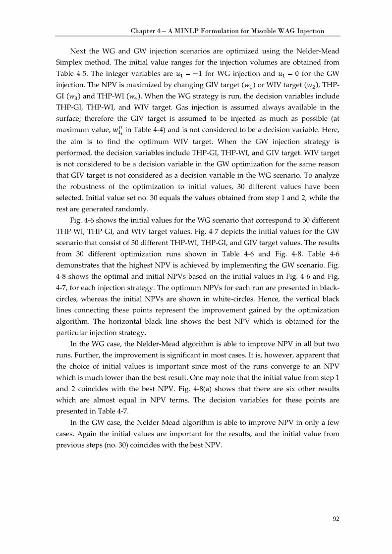
Chapter 4 – A MINLP Formulation for Miscible WAG Injection
92
Next the WG and GW injection scenarios are optimized using the Nelder-Mead Simplex method. The initial value ranges for the injection volumes are obtained from Table 4-5. The integer variables are 𝑢1 = −1 for WG injection and 𝑢1 = 0 for the GW injection. The NPV is maximized by changing GIV target (𝑤𝑤1) or WIV target (𝑤𝑤2), THP-GI (𝑤𝑤3) and THP-WI (𝑤𝑤4). When the WG strategy is run, the decision variables include THP-GI, THP-WI, and WIV target. Gas injection is assumed always available in the surface; therefore the GIV target is assumed to be injected as much as possible (at maximum value, 𝑤𝑤1𝑖
𝑈 in Table 4-4) and is not considered to be a decision variable. Here, the aim is to find the optimum WIV target. When the GW injection strategy is performed, the decision variables include THP-GI, THP-WI, and GIV target. WIV target is not considered to be a decision variable in the GW optimization for the same reason that GIV target is not considered as a decision variable in the WG scenario. To analyze the robustness of the optimization to initial values, 30 different values have been selected. Initial value set no. 30 equals the values obtained from step 1 and 2, while the rest are generated randomly.
Fig. 4-6 shows the initial values for the WG scenario that correspond to 30 different THP-WI, THP-GI, and WIV target values. Fig. 4-7 depicts the initial values for the GW scenario that consist of 30 different THP-WI, THP-GI, and GIV target values. The results from 30 different optimization runs shown in Table 4-6 and Fig. 4-8. Table 4-6 demonstrates that the highest NPV is achieved by implementing the GW scenario. Fig. 4-8 shows the optimal and initial NPVs based on the initial values in Fig. 4-6 and Fig. 4-7, for each injection strategy. The optimum NPVs for each run are presented in black-circles, whereas the initial NPVs are shown in white-circles. Hence, the vertical black lines connecting these points represent the improvement gained by the optimization algorithm. The horizontal black line shows the best NPV which is obtained for the particular injection strategy.
In the WG case, the Nelder-Mead algorithm is able to improve NPV in all but two runs. Further, the improvement is significant in most cases. It is, however, apparent that the choice of initial values is important since most of the runs converge to an NPV which is much lower than the best result. One may note that the initial value from step 1 and 2 coincides with the best NPV. Fig. 4-8(a) shows that there are six other results which are almost equal in NPV terms. The decision variables for these points are presented in Table 4-7.
In the GW case, the Nelder-Mead algorithm is able to improve NPV in only a few cases. Again the initial values are important for the results, and the initial value from previous steps (no. 30) coincides with the best NPV.
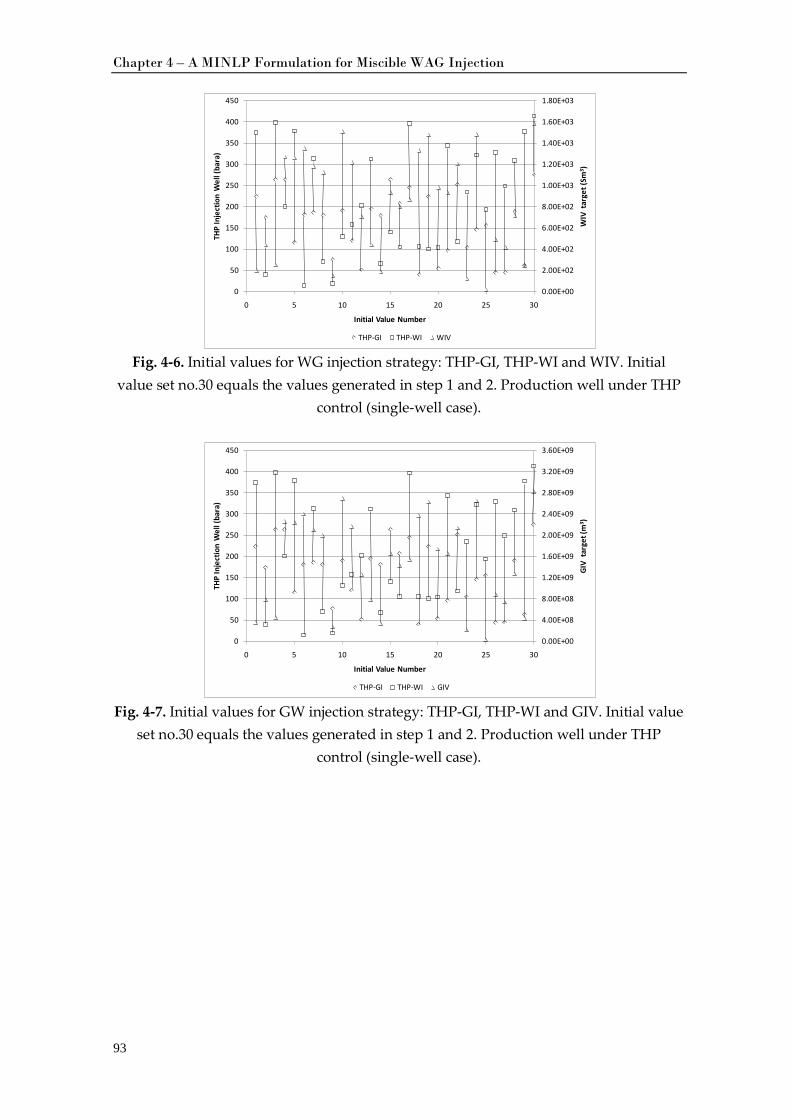
Chapter 4 – A MINLP Formulation for Miscible WAG Injection
93
Fig. 4-6. Initial values for WG injection strategy: THP-GI, THP-WI and WIV. Initial
value set no.30 equals the values generated in step 1 and 2. Production well under THP control (single-well case).
Fig. 4-7. Initial values for GW injection strategy: THP-GI, THP-WI and GIV. Initial value
set no.30 equals the values generated in step 1 and 2. Production well under THP control (single-well case).
0.00E+00
2.00E+02
4.00E+02
6.00E+02
8.00E+02
1.00E+03
1.20E+03
1.40E+03
1.60E+03
1.80E+03
0
50
100
150
200
250
300
350
400
450
0 5 10 15 20 25 30
WIV
tar
get (
Sm3 )
THP
Inje
ctio
n W
ell (
bara
)
Initial Value Number
THP-GI THP-WI WIV
0.00E+00
4.00E+08
8.00E+08
1.20E+09
1.60E+09
2.00E+09
2.40E+09
2.80E+09
3.20E+09
3.60E+09
0
50
100
150
200
250
300
350
400
450
0 5 10 15 20 25 30
GIV
targ
et (m
3 )
THP
Inje
ctio
n W
ell (
bara
)
Initial Value Number
THP-GI THP-WI GIV
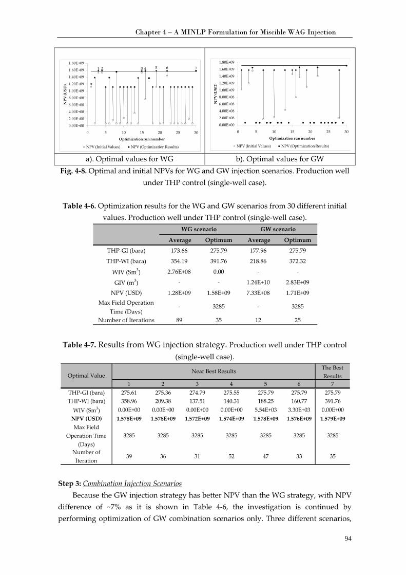
Chapter 4 – A MINLP Formulation for Miscible WAG Injection
94
a). Optimal values for WG b). Optimal values for GW
Fig. 4-8. Optimal and initial NPVs for WG and GW injection scenarios. Production well under THP control (single-well case).
Table 4-6. Optimization results for the WG and GW scenarios from 30 different initial
values. Production well under THP control (single-well case).
Table 4-7. Results from WG injection strategy. Production well under THP control (single-well case).
Step 3: Combination Injection ScenariosBecause the GW injection strategy has better NPV than the WG strategy, with NPV
difference of ~7% as it is shown in
Table 4-6, the investigation is continued by performing optimization of GW combination scenarios only. Three different scenarios,
0.00E+00
2.00E+08
4.00E+08
6.00E+08
8.00E+08
1.00E+09
1.20E+09
1.40E+09
1.60E+09
1.80E+09
0 5 10 15 20 25 30
NPV
(USD
)
Optimization run number
NPV (Initial Values) NPV (Optimization Results)
1 2 3 4 5 6 7
0.00E+00
2.00E+08
4.00E+08
6.00E+08
8.00E+08
1.00E+09
1.20E+09
1.40E+09
1.60E+09
1.80E+09
0 5 10 15 20 25 30
NPV
(USD
)
Optimization run number
NPV (Initial Values) NPV (Optimization Results)
Average Optimum Average Optimum
THP-GI (bara) 173.66 275.79 177.96 275.79
THP-WI (bara) 354.19 391.76 218.86 372.32
WIV (Sm3) 2.76E+08 0.00 - -
GIV (m3) - - 1.24E+10 2.83E+09
NPV (USD) 1.28E+09 1.58E+09 7.33E+08 1.71E+09Max Field Operation
Time (Days)- 3285 - 3285
Number of Iterations 89 35 12 25
WG scenario GW scenario
The Best Results
1 2 3 4 5 6 7THP-GI (bara) 275.61 275.36 274.79 275.55 275.79 275.79 275.79THP-WI (bara) 358.96 209.38 137.51 140.31 188.25 160.77 391.76
WIV (Sm3) 0.00E+00 0.00E+00 0.00E+00 0.00E+00 5.54E+03 3.30E+03 0.00E+00NPV (USD) 1.578E+09 1.578E+09 1.572E+09 1.574E+09 1.578E+09 1.576E+09 1.579E+09Max Field
Operation Time (Days)
3285 3285 3285 3285 3285 3285 3285
Number of Iteration
39 36 31 52 47 33 35
Optimal ValueNear Best Results
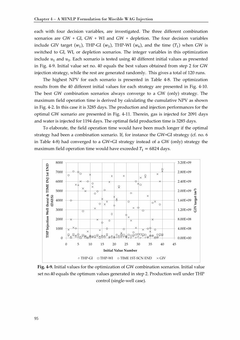
Chapter 4 – A MINLP Formulation for Miscible WAG Injection
95
each with four decision variables, are investigated. The three different combination scenarios are GW + GI, GW + WI and GW + depletion. The four decision variables include GIV target (𝑤𝑤1), THP-GI (𝑤𝑤3), THP-WI (𝑤𝑤4), and the time (𝑇𝑇1) when GW is switched to GI, WI, or depletion scenarios. The integer variables in this optimization include 𝑢1 and 𝑢3. Each scenario is tested using 40 different initial values as presented in Fig. 4-9. Initial value set no. 40 equals the best values obtained from step 2 for GW injection strategy, while the rest are generated randomly. This gives a total of 120 runs.
The highest NPV for each scenario is presented in Table 4-8. The optimization results from the 40 different initial values for each strategy are presented in Fig. 4-10. The best GW combination scenarios always converge to a GW (only) strategy. The maximum field operation time is derived by calculating the cumulative NPV as shown in Fig. 4-2. In this case it is 3285 days. The production and injection performances for the optimal GW scenario are presented in Fig. 4-11. Therein, gas is injected for 2091 days and water is injected for 1194 days. The optimal field production time is 3285 days.
To elaborate, the field operation time would have been much longer if the optimal strategy had been a combination scenario. If, for instance the GW+GI strategy (cf. no. 6 in Table 4-8) had converged to a GW+GI strategy instead of a GW (only) strategy the maximum field operation time would have exceeded 𝑇𝑇1 = 6824 days.
Fig. 4-9. Initial values for the optimization of GW combination scenarios. Initial value set no.40 equals the optimum values generated in step 2. Production well under THP
control (single-well case).
0.00E+00
4.00E+08
8.00E+08
1.20E+09
1.60E+09
2.00E+09
2.40E+09
2.80E+09
3.20E+09
0
1000
2000
3000
4000
5000
6000
7000
8000
0 5 10 15 20 25 30 35 40 45
GIV
targ
et (m
3 )
THP
Inje
ctio
n W
ell (
bara
) & T
IME
INJ 1
st E
ND
(D
AYS)
Initial Value Number
THP-GI THP-WI TIME 1ST-SCN END GIV
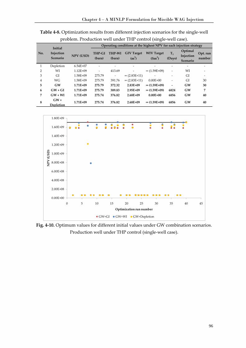
Chapter 4 – A MINLP Formulation for Miscible WAG Injection
96
Table 4-8. Optimization results from different injection scenarios for the single-well problem. Production well under THP control (single-well case).
Fig. 4-10. Optimum values for different initial values under GW combination scenarios.
Production well under THP control (single-well case).
NPV (USD)THP-GI
(bara)THP-WI
(bara)GIV Target
(m3)WIV Target
(Sm3)T1
(Days)
Optimal Injection Scenario
Opt. run number
1 Depletion 6.54E+07 - - - - - - -2 WI 1.12E+09 - 413.69 - ∞ (1.59E+09) - WI -3 GI 1.58E+09 275.79 - ∞ (2.83E+11) - - GI -4 WG 1.58E+09 275.79 391.76 ∞ (2.83E+11) 0.00E+00 - GI 305 GW 1.71E+09 275.79 372.32 2.83E+09 ∞ (1.59E+09) - GW 306 GW + GI 1.71E+09 275.79 389.83 2.95E+09 ∞ (1.59E+09) 6824 GW 77 GW + WI 1.71E+09 275.74 376.82 2.68E+09 0.00E+00 6856 GW 40
8 GW + Depletion
1.71E+09 275.74 376.82 2.68E+09 ∞ (1.59E+09) 6856 GW 40
Operating conditions at the highest NPV for each injection strategy
No.Initial
Injection Scenario
0.00E+00
2.00E+08
4.00E+08
6.00E+08
8.00E+08
1.00E+09
1.20E+09
1.40E+09
1.60E+09
1.80E+09
0 5 10 15 20 25 30 35 40 45
NPV
(USD
)
Optimization run number
GW+GI GW+WI GW+Depletion
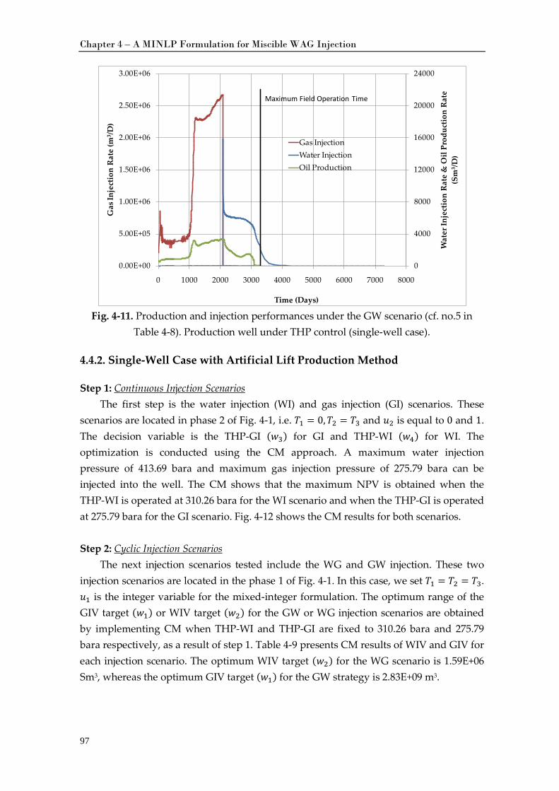
Chapter 4 – A MINLP Formulation for Miscible WAG Injection
97
Fig. 4-11. Production and injection performances under the GW scenario (cf. no.5 in
Table 4-8). Production well under THP control (single-well case).
4.4.2. Single-Well Case with Artificial Lift Production Method
Step 1: Continuous Injection ScenariosThe first step is the water injection (WI) and gas injection (GI) scenarios. These
scenarios are located in phase 2 of
Fig. 4-1, i.e. 𝑇𝑇1 = 0,𝑇𝑇2 = 𝑇𝑇3 and 𝑢2 is equal to 0 and 1. The decision variable is the THP-GI (𝑤𝑤3) for GI and THP-WI (𝑤𝑤4) for WI. The optimization is conducted using the CM approach. A maximum water injection pressure of 413.69 bara and maximum gas injection pressure of 275.79 bara can be injected into the well. The CM shows that the maximum NPV is obtained when the THP-WI is operated at 310.26 bara for the WI scenario and when the THP-GI is operated at 275.79 bara for the GI scenario. Fig. 4-12 shows the CM results for both scenarios. Step 2: Cyclic Injection Scenarios
The next injection scenarios tested include the WG and GW injection. These two injection scenarios are located in the phase 1 of
Fig. 4-1. In this case, we set 𝑇𝑇1 = 𝑇𝑇2 = 𝑇𝑇3. 𝑢1 is the integer variable for the mixed-integer formulation. The optimum range of the GIV target (𝑤𝑤1) or WIV target (𝑤𝑤2) for the GW or WG injection scenarios are obtained by implementing CM when THP-WI and THP-GI are fixed to 310.26 bara and 275.79 bara respectively, as a result of step 1. Table 4-9 presents CM results of WIV and GIV for each injection scenario. The optimum WIV target (𝑤𝑤2) for the WG scenario is 1.59E+06 Sm3, whereas the optimum GIV target (𝑤𝑤1) for the GW strategy is 2.83E+09 m3.
0
4000
8000
12000
16000
20000
24000
0.00E+00
5.00E+05
1.00E+06
1.50E+06
2.00E+06
2.50E+06
3.00E+06
0 1000 2000 3000 4000 5000 6000 7000 8000
Wat
er In
ject
ion
Rat
e &
Oil
Prod
uctio
n R
ate
(Sm
3 /D)
Gas
Inje
ctio
n R
ate
(m3 /D
)
Time (Days)
Gas InjectionWater InjectionOil Production
Maximum Field Operation Time
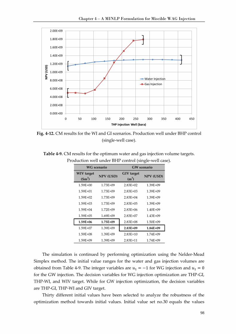
Chapter 4 – A MINLP Formulation for Miscible WAG Injection
98
Fig. 4-12. CM results for the WI and GI scenarios. Production well under BHP control
(single-well case). Table 4-9. CM results for the optimum water and gas injection volume targets.
Production well under BHP control (single-well case).
The simulation is continued by performing optimization using the Nelder-Mead Simplex method. The initial value ranges for the water and gas injection volumes are obtained from Table 4-9. The integer variables are 𝑢1 = −1 for WG injection and 𝑢1 = 0 for the GW injection. The decision variables for WG injection optimization are THP-GI, THP-WI, and WIV target. While for GW injection optimization, the decision variables are THP-GI, THP-WI and GIV target.
Thirty different initial values have been selected to analyze the robustness of the optimization method towards initial values. Initial value set no.30 equals the values
0.00E+00
2.00E+08
4.00E+08
6.00E+08
8.00E+08
1.00E+09
1.20E+09
1.40E+09
1.60E+09
1.80E+09
2.00E+09
0 50 100 150 200 250 300 350 400 450
NPV
(USD
)
THP Injection Well (bara)
Water InjectionGas Injection
WIV target (Sm3)
NPV (USD)GIV target
(m3)NPV (USD)
1.59E+00 1.73E+09 2.83E+02 1.39E+09
1.59E+01 1.73E+09 2.83E+03 1.39E+09
1.59E+02 1.73E+09 2.83E+04 1.39E+09
1.59E+03 1.73E+09 2.83E+05 1.39E+09
1.59E+04 1.72E+09 2.83E+06 1.40E+09
1.59E+05 1.69E+09 2.83E+07 1.43E+09
1.59E+06 1.75E+09 2.83E+08 1.50E+09
1.59E+07 1.39E+09 2.83E+09 1.84E+09
1.59E+08 1.39E+09 2.83E+10 1.74E+09
1.59E+09 1.39E+09 2.83E+11 1.74E+09
WG scenario GW scenario
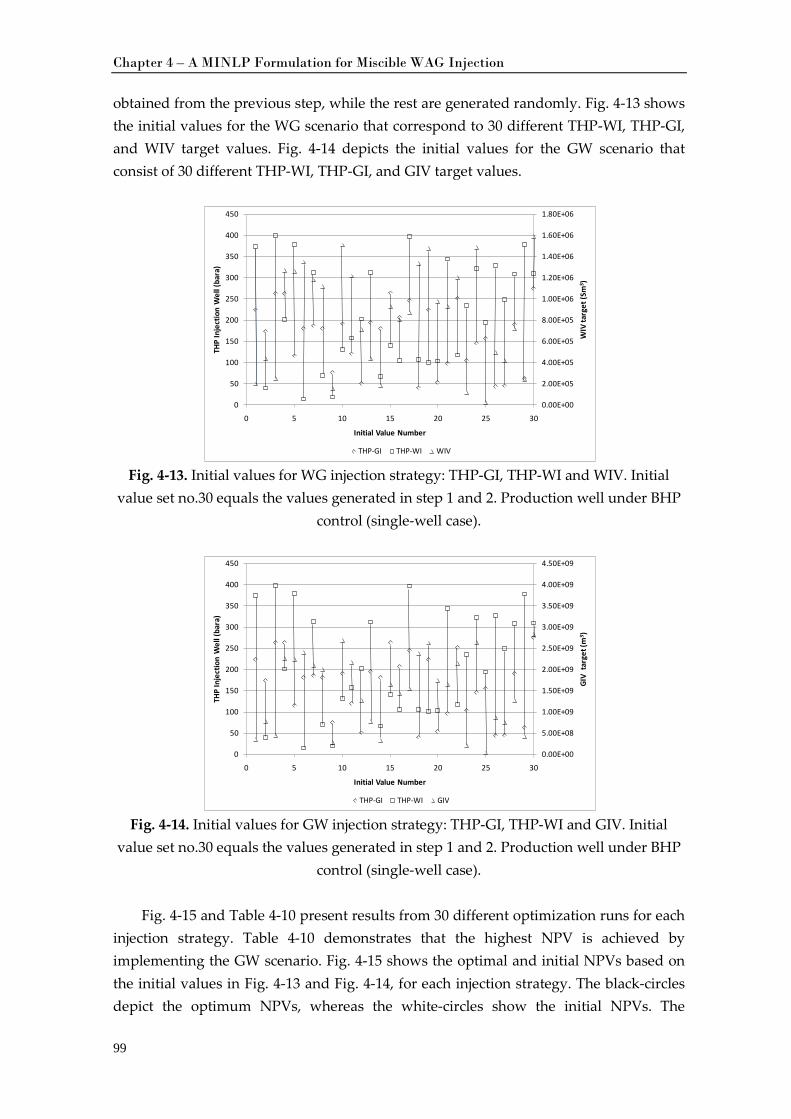
Chapter 4 – A MINLP Formulation for Miscible WAG Injection
99
obtained from the previous step, while the rest are generated randomly. Fig. 4-13 shows the initial values for the WG scenario that correspond to 30 different THP-WI, THP-GI, and WIV target values. Fig. 4-14 depicts the initial values for the GW scenario that consist of 30 different THP-WI, THP-GI, and GIV target values.
Fig. 4-13. Initial values for WG injection strategy: THP-GI, THP-WI and WIV. Initial
value set no.30 equals the values generated in step 1 and 2. Production well under BHP control (single-well case).
Fig. 4-14. Initial values for GW injection strategy: THP-GI, THP-WI and GIV. Initial
value set no.30 equals the values generated in step 1 and 2. Production well under BHP control (single-well case).
Fig. 4-15 and Table 4-10 present results from 30 different optimization runs for each
injection strategy. Table 4-10 demonstrates that the highest NPV is achieved by implementing the GW scenario. Fig. 4-15 shows the optimal and initial NPVs based on the initial values in Fig. 4-13 and Fig. 4-14, for each injection strategy. The black-circles depict the optimum NPVs, whereas the white-circles show the initial NPVs. The
0.00E+00
2.00E+05
4.00E+05
6.00E+05
8.00E+05
1.00E+06
1.20E+06
1.40E+06
1.60E+06
1.80E+06
0
50
100
150
200
250
300
350
400
450
0 5 10 15 20 25 30
WIV
targ
et (S
m3 )
THP
Inje
ctio
n W
ell (
bara
)
Initial Value Number
THP-GI THP-WI WIV
0.00E+00
5.00E+08
1.00E+09
1.50E+09
2.00E+09
2.50E+09
3.00E+09
3.50E+09
4.00E+09
4.50E+09
0
50
100
150
200
250
300
350
400
450
0 5 10 15 20 25 30
GIV
targ
et (m
3 )
THP
Inje
ctio
n W
ell (
bara
)
Initial Value Number
THP-GI THP-WI GIV
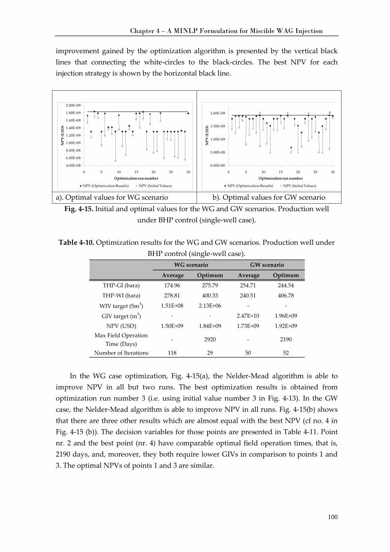
Chapter 4 – A MINLP Formulation for Miscible WAG Injection
100
improvement gained by the optimization algorithm is presented by the vertical black lines that connecting the white-circles to the black-circles. The best NPV for each injection strategy is shown by the horizontal black line.
a). Optimal values for WG scenario b). Optimal values for GW scenario
Fig. 4-15. Initial and optimal values for the WG and GW scenarios. Production well under BHP control (single-well case).
Table 4-10. Optimization results for the WG and GW scenarios. Production well under
BHP control (single-well case).
In the WG case optimization, Fig. 4-15(a), the Nelder-Mead algorithm is able to
improve NPV in all but two runs. The best optimization results is obtained from optimization run number 3 (i.e. using initial value number 3 in Fig. 4-13). In the GW case, the Nelder-Mead algorithm is able to improve NPV in all runs. Fig. 4-15(b) shows that there are three other results which are almost equal with the best NPV (cf no. 4 in Fig. 4-15 (b)). The decision variables for those points are presented in Table 4-11. Point nr. 2 and the best point (nr. 4) have comparable optimal field operation times, that is, 2190 days, and, moreover, they both require lower GIVs in comparison to points 1 and 3. The optimal NPVs of points 1 and 3 are similar.
4.00E+08
6.00E+08
8.00E+08
1.00E+09
1.20E+09
1.40E+09
1.60E+09
1.80E+09
2.00E+09
0 5 10 15 20 25 30
NPV
(USD
)
Optimization run number
NPV (Optimization Results) NPV (Initial Values)
1 4
0.00E+00
5.00E+08
1.00E+09
1.50E+09
2.00E+09
0 5 10 15 20 25 30
NPV
(USD
)
Optimization run number
NPV (Optimization Results) NPV (Initial Values)
2 3
Average Optimum Average Optimum
THP-GI (bara) 174.96 275.79 254.71 244.54
THP-WI (bara) 278.81 400.33 240.51 406.78
WIV target (Sm3) 1.51E+08 2.13E+06 - -
GIV target (m3) - - 2.47E+10 1.96E+09
NPV (USD) 1.50E+09 1.84E+09 1.73E+09 1.92E+09Max Field Operation
Time (Days)- 2920 - 2190
Number of Iterations 118 29 50 52
WG scenario GW scenario
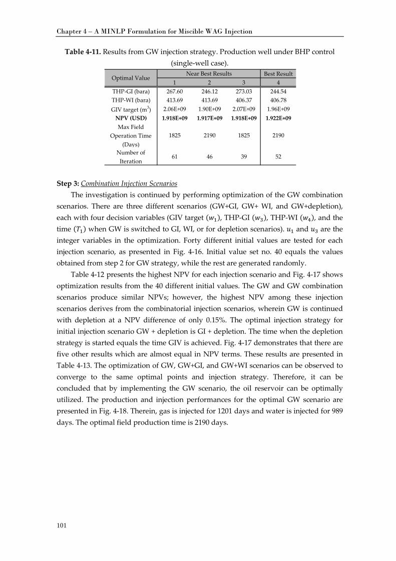
Chapter 4 – A MINLP Formulation for Miscible WAG Injection
101
Table 4-11. Results from GW injection strategy. Production well under BHP control (single-well case).
Step 3: Combination Injection ScenariosThe investigation is continued by performing optimization of the GW combination
scenarios. There are three different scenarios (GW+GI, GW+ WI, and GW+depletion), each with four decision variables (GIV target (𝑤𝑤1), THP-GI (𝑤𝑤3), THP-WI (𝑤𝑤4), and the time (𝑇𝑇1) when GW is switched to GI, WI, or for depletion scenarios). 𝑢1 and 𝑢3 are the integer variables in the optimization. Forty different initial values are tested for each injection scenario, as presented in
Fig. 4-16. Initial value set no. 40 equals the values obtained from step 2 for GW strategy, while the rest are generated randomly.
Table 4-12 presents the highest NPV for each injection scenario and Fig. 4-17 shows optimization results from the 40 different initial values. The GW and GW combination scenarios produce similar NPVs; however, the highest NPV among these injection scenarios derives from the combinatorial injection scenarios, wherein GW is continued with depletion at a NPV difference of only 0.15%. The optimal injection strategy for initial injection scenario GW + depletion is GI + depletion. The time when the depletion strategy is started equals the time GIV is achieved. Fig. 4-17 demonstrates that there are five other results which are almost equal in NPV terms. These results are presented in Table 4-13. The optimization of GW, GW+GI, and GW+WI scenarios can be observed to converge to the same optimal points and injection strategy. Therefore, it can be concluded that by implementing the GW scenario, the oil reservoir can be optimally utilized. The production and injection performances for the optimal GW scenario are presented in Fig. 4-18. Therein, gas is injected for 1201 days and water is injected for 989 days. The optimal field production time is 2190 days.
Best Result1 2 3 4
THP-GI (bara) 267.60 246.12 273.03 244.54THP-WI (bara) 413.69 413.69 406.37 406.78GIV target (m3) 2.06E+09 1.90E+09 2.07E+09 1.96E+09
NPV (USD) 1.918E+09 1.917E+09 1.918E+09 1.922E+09Max Field
Operation Time (Days)
1825 2190 1825 2190
Number of Iteration
61 46 39 52
Optimal ValueNear Best Results
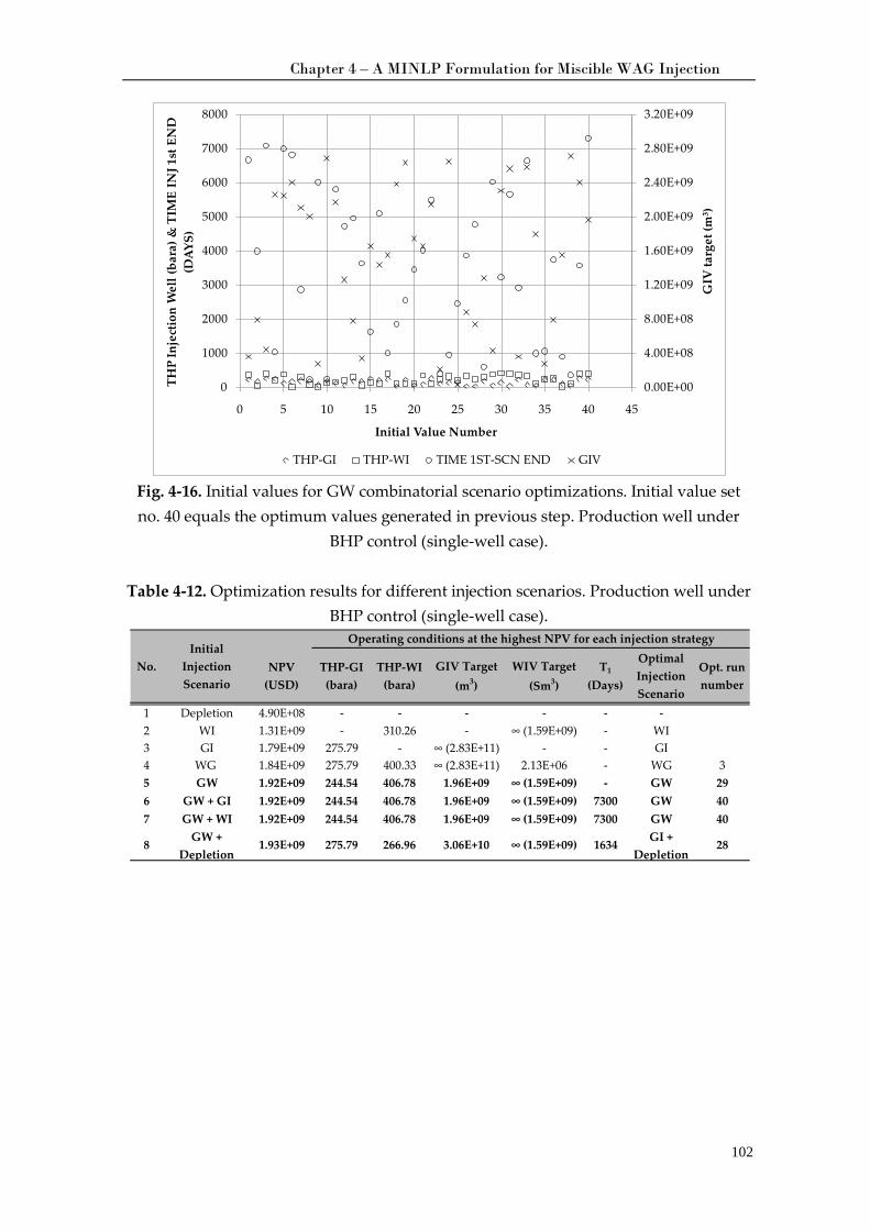
Chapter 4 – A MINLP Formulation for Miscible WAG Injection
102
Fig. 4-16. Initial values for GW combinatorial scenario optimizations. Initial value set no. 40 equals the optimum values generated in previous step. Production well under
BHP control (single-well case).
Table 4-12. Optimization results for different injection scenarios. Production well under BHP control (single-well case).
0.00E+00
4.00E+08
8.00E+08
1.20E+09
1.60E+09
2.00E+09
2.40E+09
2.80E+09
3.20E+09
0
1000
2000
3000
4000
5000
6000
7000
8000
0 5 10 15 20 25 30 35 40 45
GIV
targ
et (m
3 )
THP
Inje
ctio
n W
ell (
bara
) & T
IME
INJ 1
st E
ND
(D
AYS)
Initial Value Number
THP-GI THP-WI TIME 1ST-SCN END GIV
NPV (USD)
THP-GI (bara)
THP-WI (bara)
GIV Target (m3)
WIV Target (Sm3)
T1
(Days)
Optimal Injection Scenario
Opt. run number
1 Depletion 4.90E+08 - - - - - -2 WI 1.31E+09 - 310.26 - ∞ (1.59E+09) - WI3 GI 1.79E+09 275.79 - ∞ (2.83E+11) - - GI4 WG 1.84E+09 275.79 400.33 ∞ (2.83E+11) 2.13E+06 - WG 35 GW 1.92E+09 244.54 406.78 1.96E+09 ∞ (1.59E+09) - GW 296 GW + GI 1.92E+09 244.54 406.78 1.96E+09 ∞ (1.59E+09) 7300 GW 407 GW + WI 1.92E+09 244.54 406.78 1.96E+09 ∞ (1.59E+09) 7300 GW 40
8 GW + Depletion
1.93E+09 275.79 266.96 3.06E+10 ∞ (1.59E+09) 1634 GI + Depletion
28
Operating conditions at the highest NPV for each injection strategy
No.Initial
Injection Scenario
Chapter 4 – A MINLP Formulation for Miscible WAG Injection
103
Fig. 4-17. Optimum values for the GW combinatorial scenarios for a single-well case.
Production well under BHP control (single-well case).
Table 4-13. Optimum results at the highest NPV point and near the highest NPV points for GW+depletion injection scenario. Production well under BHP control (single-well
case).
4.00E+08
6.00E+08
8.00E+08
1.00E+09
1.20E+09
1.40E+09
1.60E+09
1.80E+09
2.00E+09
2.20E+09
0 5 10 15 20 25 30 35 40 45
NPV
(USD
)
Optimization run number
GW+GI GW+WI GW+Depletion
1 2 3 4 56
Best Point1 2 3 4 5 6
THP-GI (bara) 275.79 245.70 275.79 275.79 244.54 275.79THP-WI (bara) 150.66 396.84 126.10 242.81 406.78 266.96GIV Target (m3) 4.00E+10 1.55E+09 1.43E+11 3.14E+10 1.96E+09 3.06E+10Time 1st Inj Scn
End (days)1729 1742 1706 1677 7300 1634
NPV (USD) 1.923E+09 1.924E+09 1.924E+09 1.925E+09 1.922E+09 1.925E+09Max Field
Operation Time (Days)
3285 4745 3285 3285 2190 3285
Number of Iteration
28 27 41 35 38 29
Optimal ValueNear Best Point
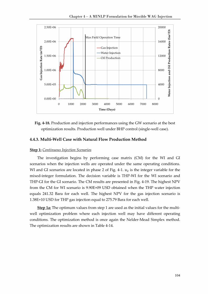
Chapter 4 – A MINLP Formulation for Miscible WAG Injection
104
Fig. 4-18. Production and injection performances using the GW scenario at the best optimization results. Production well under BHP control (single-well case).
4.4.3. Multi-Well Case with Natural Flow Production Method
Step 1:
The investigation begins by performing case matrix (CM) for the WI and GI scenarios when the injection wells are operated under the same operating conditions. WI and GI scenarios are located in phase 2 of
Continuous Injection Scenarios
Fig. 4-1. 𝑢2 is the integer variable for the mixed-integer formulation. The decision variable is THP-WI for the WI scenario and THP-GI for the GI scenario. The CM results are presented in Fig. 4-19. The highest NPV from the CM for WI scenario is 9.90E+09 USD obtained when the THP water injection equals 241.32 Bara for each well. The highest NPV for the gas injection scenario is 1.38E+10 USD for THP gas injection equal to 275.79 Bara for each well.
Step 1a:
Table 4-14
The optimum values from step 1 are used as the initial values for the multi-well optimization problem where each injection well may have different operating conditions. The optimization method is once again the Nelder-Mead Simplex method. The optimization results are shown in .
0
4000
8000
12000
16000
20000
0.00E+00
5.00E+05
1.00E+06
1.50E+06
2.00E+06
2.50E+06
0 1000 2000 3000 4000 5000 6000 7000 8000
Wat
er In
ject
ion
and
Oil
Prod
uctio
n R
ates
(Sm
3 /D)
Gas
Inje
ctio
n R
ate
(m3 /D
)
Time (Days)
Gas Injection
Water Injection
Oil Production
Max Field Operation Time
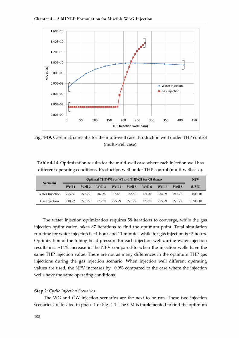
Chapter 4 – A MINLP Formulation for Miscible WAG Injection
105
Fig. 4-19. Case matrix results for the multi-well case. Production well under THP control
(multi-well case).
Table 4-14. Optimization results for the multi-well case where each injection well has different operating conditions. Production well under THP control (multi-well case).
The water injection optimization requires 58 iterations to converge, while the gas injection optimization takes 87 iterations to find the optimum point. Total simulation run time for water injection is ~1 hour and 11 minutes while for gas injection is ~5 hours. Optimization of the tubing head pressure for each injection well during water injection results in a ~14% increase in the NPV compared to when the injection wells have the same THP injection value. There are not as many differences in the optimum THP gas injections during the gas injection scenario. When injection well different operating values are used, the NPV increases by ~0.9% compared to the case where the injection wells have the same operating conditions.
Step 2:
The WG and GW injection scenarios are the next to be run. These two injection scenarios are located in phase 1 of
Cyclic Injection Scenarios
Fig. 4-1. The CM is implemented to find the optimum
0.00E+00
2.00E+09
4.00E+09
6.00E+09
8.00E+09
1.00E+10
1.20E+10
1.40E+10
1.60E+10
0 50 100 150 200 250 300 350 400 450
NPV
(USD
)
THP Injection Well (bara)
Water InjectionGas Injection
NPV
Well 1 Well 2 Well 3 Well 4 Well 5 Well 6 Well 7 Well 8 (USD)
Water Injection 295.86 275.79 282.25 37.48 163.50 274.30 324.69 242.28 1.15E+10
Gas Injection 248.22 275.79 275.79 275.79 275.79 275.79 275.79 275.79 1.39E+10
ScenarioOptimal THP-WI for WI and THP-GI for GI (bara)
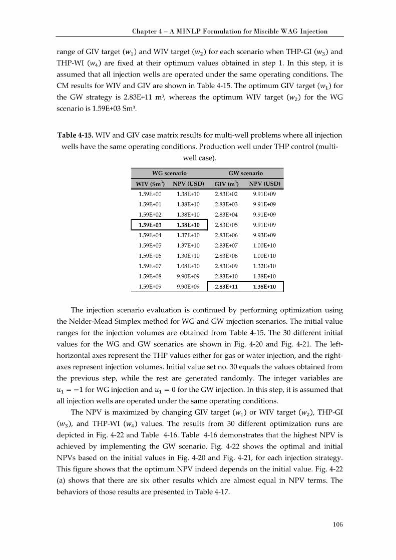
Chapter 4 – A MINLP Formulation for Miscible WAG Injection
106
range of GIV target (𝑤𝑤1) and WIV target (𝑤𝑤2) for each scenario when THP-GI (𝑤𝑤3) and THP-WI (𝑤𝑤4) are fixed at their optimum values obtained in step 1. In this step, it is assumed that all injection wells are operated under the same operating conditions. The CM results for WIV and GIV are shown in Table 4-15. The optimum GIV target (𝑤𝑤1) for the GW strategy is 2.83E+11 m3, whereas the optimum WIV target (𝑤𝑤2) for the WG scenario is 1.59E+03 Sm3.
Table 4-15. WIV and GIV case matrix results for multi-well problems where all injection wells have the same operating conditions. Production well under THP control (multi-
well case).
The injection scenario evaluation is continued by performing optimization using
the Nelder-Mead Simplex method for WG and GW injection scenarios. The initial value ranges for the injection volumes are obtained from Table 4-15. The 30 different initial values for the WG and GW scenarios are shown in Fig. 4-20 and Fig. 4-21. The left-horizontal axes represent the THP values either for gas or water injection, and the right-axes represent injection volumes. Initial value set no. 30 equals the values obtained from the previous step, while the rest are generated randomly. The integer variables are 𝑢1 = −1 for WG injection and 𝑢1 = 0 for the GW injection. In this step, it is assumed that all injection wells are operated under the same operating conditions.
The NPV is maximized by changing GIV target (𝑤𝑤1) or WIV target (𝑤𝑤2), THP-GI (𝑤𝑤3), and THP-WI (𝑤𝑤4) values. The results from 30 different optimization runs are depicted in Fig. 4-22 and Table 4-16. Table 4-16 demonstrates that the highest NPV is achieved by implementing the GW scenario. Fig. 4-22 shows the optimal and initial NPVs based on the initial values in Fig. 4-20 and Fig. 4-21, for each injection strategy. This figure shows that the optimum NPV indeed depends on the initial value. Fig. 4-22 (a) shows that there are six other results which are almost equal in NPV terms. The behaviors of those results are presented in Table 4-17.
WIV (Sm3) NPV (USD) GIV (m3) NPV (USD)
1.59E+00 1.38E+10 2.83E+02 9.91E+09
1.59E+01 1.38E+10 2.83E+03 9.91E+09
1.59E+02 1.38E+10 2.83E+04 9.91E+09
1.59E+03 1.38E+10 2.83E+05 9.91E+09
1.59E+04 1.37E+10 2.83E+06 9.93E+09
1.59E+05 1.37E+10 2.83E+07 1.00E+10
1.59E+06 1.30E+10 2.83E+08 1.00E+10
1.59E+07 1.08E+10 2.83E+09 1.32E+10
1.59E+08 9.90E+09 2.83E+10 1.38E+10
1.59E+09 9.90E+09 2.83E+11 1.38E+10
WG scenario GW scenario
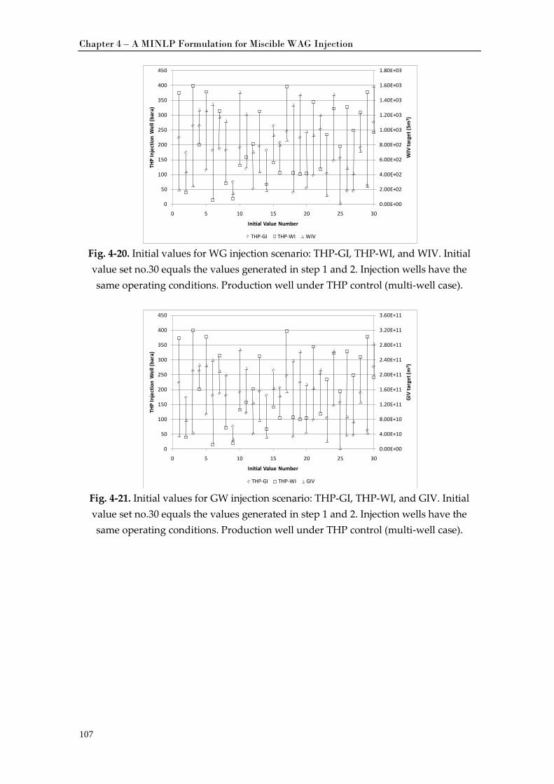
Chapter 4 – A MINLP Formulation for Miscible WAG Injection
107
Fig. 4-20. Initial values for WG injection scenario: THP-GI, THP-WI, and WIV. Initial value set no.30 equals the values generated in step 1 and 2. Injection wells have the same operating conditions. Production well under THP control (multi-well case).
Fig. 4-21. Initial values for GW injection scenario: THP-GI, THP-WI, and GIV. Initial value set no.30 equals the values generated in step 1 and 2. Injection wells have the same operating conditions. Production well under THP control (multi-well case).
0.00E+00
2.00E+02
4.00E+02
6.00E+02
8.00E+02
1.00E+03
1.20E+03
1.40E+03
1.60E+03
1.80E+03
0
50
100
150
200
250
300
350
400
450
0 5 10 15 20 25 30
WIV
targ
et (S
m3 )
THP
Inje
ctio
n W
ell (
bara
)
Initial Value Number
THP-GI THP-WI WIV
0.00E+00
4.00E+10
8.00E+10
1.20E+11
1.60E+11
2.00E+11
2.40E+11
2.80E+11
3.20E+11
3.60E+11
0
50
100
150
200
250
300
350
400
450
0 5 10 15 20 25 30
GIV
targ
et (m
3 )
THP
Inje
ctio
n W
ell (
bara
)
Initial Value Number
THP-GI THP-WI GIV
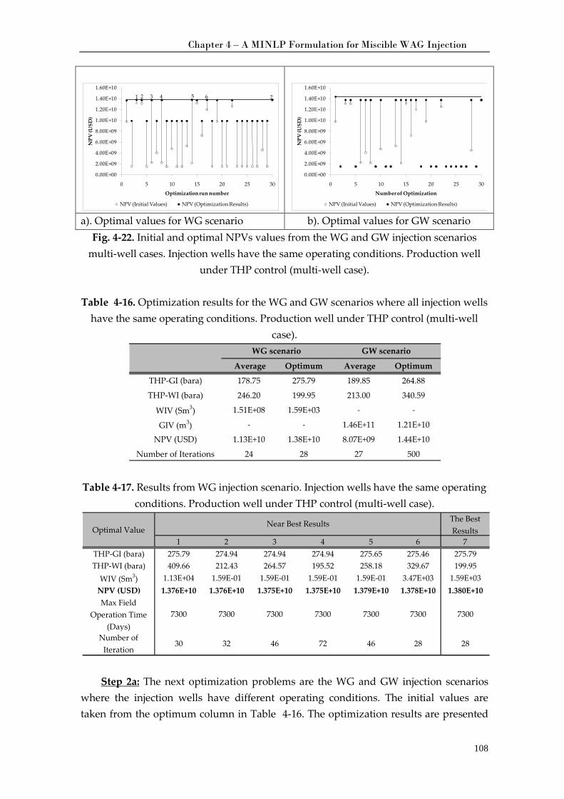
Chapter 4 – A MINLP Formulation for Miscible WAG Injection
108
a). Optimal values for WG scenario b). Optimal values for GW scenario
Fig. 4-22. Initial and optimal NPVs values from the WG and GW injection scenarios multi-well cases. Injection wells have the same operating conditions. Production well
under THP control (multi-well case).
Table 4-16. Optimization results for the WG and GW scenarios where all injection wells have the same operating conditions. Production well under THP control (multi-well
case).
Table 4-17. Results from WG injection scenario. Injection wells have the same operating conditions. Production well under THP control (multi-well case).
Step 2a:
Table 4-16
The next optimization problems are the WG and GW injection scenarios where the injection wells have different operating conditions. The initial values are taken from the optimum column in . The optimization results are presented
0.00E+00
2.00E+09
4.00E+09
6.00E+09
8.00E+09
1.00E+10
1.20E+10
1.40E+10
1.60E+10
0 5 10 15 20 25 30
NPV
(USD
)
Optimization run number
NPV (Initial Values) NPV (Optimization Results)
1 2 3 4 5 6 7
0.00E+00
2.00E+09
4.00E+09
6.00E+09
8.00E+09
1.00E+10
1.20E+10
1.40E+10
1.60E+10
0 5 10 15 20 25 30
NPV
(USD
)
Number of Optimization
NPV (Initial Values) NPV (Optimization Results)
Average Optimum Average Optimum
THP-GI (bara) 178.75 275.79 189.85 264.88
THP-WI (bara) 246.20 199.95 213.00 340.59
WIV (Sm3) 1.51E+08 1.59E+03 - -
GIV (m3) - - 1.46E+11 1.21E+10
NPV (USD) 1.13E+10 1.38E+10 8.07E+09 1.44E+10
Number of Iterations 24 28 27 500
WG scenario GW scenario
The Best Results
1 2 3 4 5 6 7THP-GI (bara) 275.79 274.94 274.94 274.94 275.65 275.46 275.79THP-WI (bara) 409.66 212.43 264.57 195.52 258.18 329.67 199.95
WIV (Sm3) 1.13E+04 1.59E-01 1.59E-01 1.59E-01 1.59E-01 3.47E+03 1.59E+03NPV (USD) 1.376E+10 1.376E+10 1.375E+10 1.375E+10 1.379E+10 1.378E+10 1.380E+10Max Field
Operation Time (Days)
7300 7300 7300 7300 7300 7300 7300
Number of Iteration
30 32 46 72 46 28 28
Optimal ValueNear Best Results
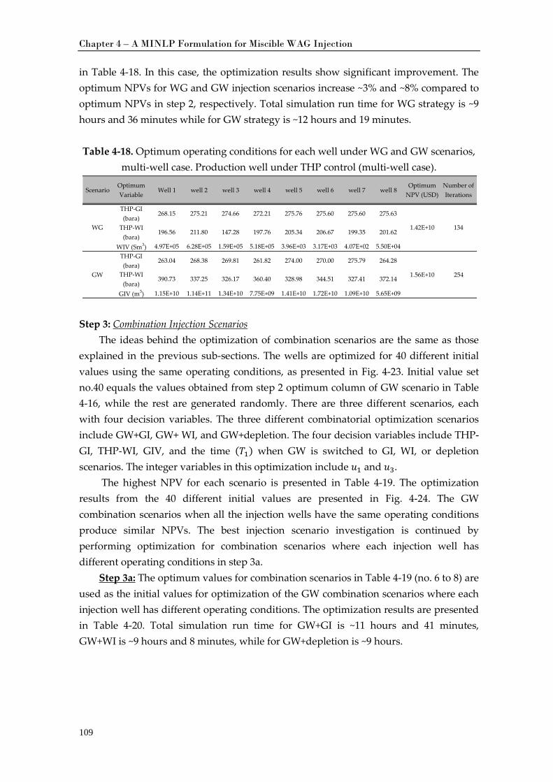
Chapter 4 – A MINLP Formulation for Miscible WAG Injection
109
in Table 4-18. In this case, the optimization results show significant improvement. The optimum NPVs for WG and GW injection scenarios increase ~3% and ~8% compared to optimum NPVs in step 2, respectively. Total simulation run time for WG strategy is ~9 hours and 36 minutes while for GW strategy is ~12 hours and 19 minutes.
Table 4-18. Optimum operating conditions for each well under WG and GW scenarios,
multi-well case. Production well under THP control (multi-well case).
Step 3: The ideas behind the optimization of combination scenarios are the same as those
explained in the previous sub-sections. The wells are optimized for 40 different initial values using the same operating conditions, as presented in
Combination Injection Scenarios
Fig. 4-23. Initial value set no.40 equals the values obtained from step 2 optimum column of GW scenario in Table 4-16, while the rest are generated randomly. There are three different scenarios, each with four decision variables. The three different combinatorial optimization scenarios include GW+GI, GW+ WI, and GW+depletion. The four decision variables include THP-GI, THP-WI, GIV, and the time (𝑇𝑇1) when GW is switched to GI, WI, or depletion scenarios. The integer variables in this optimization include 𝑢1 and 𝑢3.
The highest NPV for each scenario is presented in Table 4-19. The optimization results from the 40 different initial values are presented in Fig. 4-24. The GW combination scenarios when all the injection wells have the same operating conditions produce similar NPVs. The best injection scenario investigation is continued by performing optimization for combination scenarios where each injection well has different operating conditions in step 3a.
Step 3a: Table 4-19 The optimum values for combination scenarios in (no. 6 to 8) are used as the initial values for optimization of the GW combination scenarios where each injection well has different operating conditions. The optimization results are presented in Table 4-20. Total simulation run time for GW+GI is ~11 hours and 41 minutes, GW+WI is ~9 hours and 8 minutes, while for GW+depletion is ~9 hours.
ScenarioOptimum Variable
Well 1 well 2 well 3 well 4 well 5 well 6 well 7 well 8Optimum
NPV (USD)Number of Iterations
THP-GI (bara)
268.15 275.21 274.66 272.21 275.76 275.60 275.60 275.63
THP-WI (bara)
196.56 211.80 147.28 197.76 205.34 206.67 199.35 201.62
WIV (Sm3) 4.97E+05 6.28E+05 1.59E+05 5.18E+05 3.96E+03 3.17E+03 4.07E+02 5.50E+04THP-GI (bara)
263.04 268.38 269.81 261.82 274.00 270.00 275.79 264.28
THP-WI (bara)
390.73 337.25 326.17 360.40 328.98 344.51 327.41 372.14
GIV (m3) 1.15E+10 1.14E+11 1.34E+10 7.75E+09 1.41E+10 1.72E+10 1.09E+10 5.65E+09
WG 1.42E+10 134
GW 1.56E+10 254
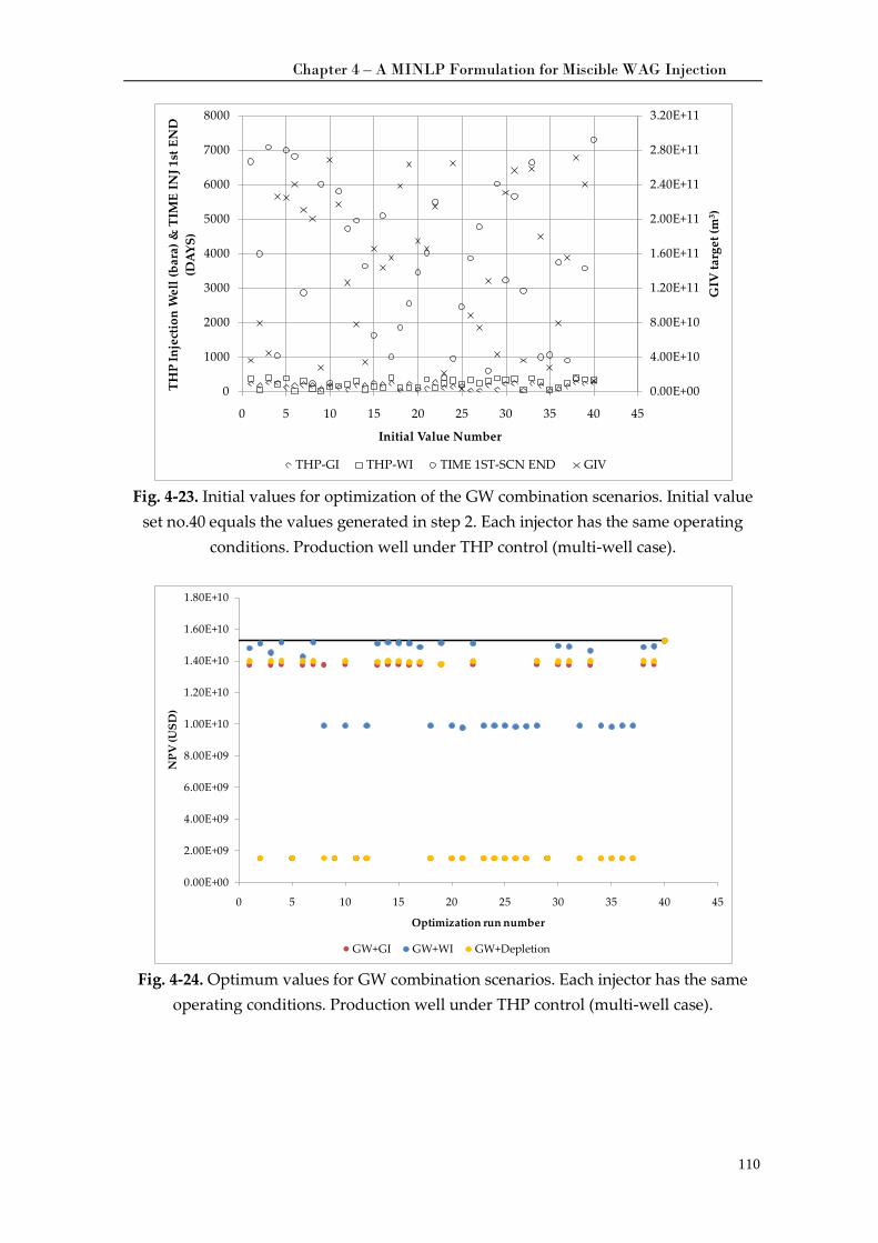
Chapter 4 – A MINLP Formulation for Miscible WAG Injection
110
Fig. 4-23. Initial values for optimization of the GW combination scenarios. Initial value
set no.40 equals the values generated in step 2. Each injector has the same operating conditions. Production well under THP control (multi-well case).
Fig. 4-24. Optimum values for GW combination scenarios. Each injector has the same
operating conditions. Production well under THP control (multi-well case).
0.00E+00
4.00E+10
8.00E+10
1.20E+11
1.60E+11
2.00E+11
2.40E+11
2.80E+11
3.20E+11
0
1000
2000
3000
4000
5000
6000
7000
8000
0 5 10 15 20 25 30 35 40 45
GIV
targ
et (m
3 )
THP
Inje
ctio
n W
ell (
bara
) & T
IME
INJ 1
st E
ND
(D
AYS)
Initial Value Number
THP-GI THP-WI TIME 1ST-SCN END GIV
0.00E+00
2.00E+09
4.00E+09
6.00E+09
8.00E+09
1.00E+10
1.20E+10
1.40E+10
1.60E+10
1.80E+10
0 5 10 15 20 25 30 35 40 45
NPV
(USD
)
Optimization run number
GW+GI GW+WI GW+Depletion
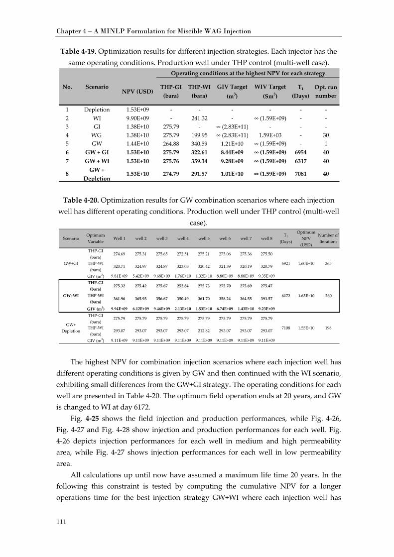
Chapter 4 – A MINLP Formulation for Miscible WAG Injection
111
Table 4-19. Optimization results for different injection strategies. Each injector has the same operating conditions. Production well under THP control (multi-well case).
Table 4-20. Optimization results for GW combination scenarios where each injection well has different operating conditions. Production well under THP control (multi-well
case).
The highest NPV for combination injection scenarios where each injection well has different operating conditions is given by GW and then continued with the WI scenario, exhibiting small differences from the GW+GI strategy. The operating conditions for each well are presented in Table 4-20. The optimum field operation ends at 20 years, and GW is changed to WI at day 6172.
Fig. 4-25 shows the field injection and production performances, while Fig. 4-26, Fig. 4-27 and Fig. 4-28 show injection and production performances for each well. Fig. 4-26 depicts injection performances for each well in medium and high permeability area, while Fig. 4-27 shows injection performances for each well in low permeability area.
All calculations up until now have assumed a maximum life time 20 years. In the following this constraint is tested by computing the cumulative NPV for a longer operations time for the best injection strategy GW+WI where each injection well has
NPV (USD)THP-GI (bara)
THP-WI (bara)
GIV Target (m3)
WIV Target (Sm3)
T1
(Days)Opt. run number
1 Depletion 1.53E+09 - - - - - -2 WI 9.90E+09 - 241.32 - ∞ (1.59E+09) - -3 GI 1.38E+10 275.79 - ∞ (2.83E+11) - - -4 WG 1.38E+10 275.79 199.95 ∞ (2.83E+11) 1.59E+03 - 305 GW 1.44E+10 264.88 340.59 1.21E+10 ∞ (1.59E+09) - 16 GW + GI 1.53E+10 275.79 322.61 8.44E+09 ∞ (1.59E+09) 6954 407 GW + WI 1.53E+10 275.76 359.34 9.28E+09 ∞ (1.59E+09) 6317 40
8 GW + Depletion
1.53E+10 274.79 291.57 1.01E+10 ∞ (1.59E+09) 7081 40
Operating conditions at the highest NPV for each strategy
No. Scenario
ScenarioOptimum Variable
Well 1 well 2 well 3 well 4 well 5 well 6 well 7 well 8T1
(Days)
Optimum NPV
(USD)
Number of Iterations
THP-GI (bara)
274.69 275.31 275.65 272.51 275.21 275.06 275.36 275.50
THP-WI (bara)
320.71 324.97 324.87 323.03 320.42 321.39 320.19 320.79
GIV (m3) 9.81E+09 5.42E+09 9.68E+09 1.76E+10 1.32E+10 8.80E+09 8.88E+09 9.35E+09THP-GI (bara)
275.32 275.42 275.67 252.84 275.73 275.70 275.69 275.47
THP-WI (bara)
361.96 365.93 356.67 350.49 361.70 358.24 364.55 391.57
GIV (m3) 9.94E+09 6.12E+09 9.46E+09 2.13E+10 1.53E+10 6.74E+09 1.43E+10 9.23E+09THP-GI (bara)
275.79 275.79 275.79 275.79 275.79 275.79 275.79 275.79
THP-WI (bara)
293.07 293.07 293.07 293.07 212.82 293.07 293.07 293.07
GIV (m3) 9.11E+09 9.11E+09 9.11E+09 9.11E+09 9.11E+09 9.11E+09 9.11E+09 9.11E+09
GW+ Depletion
1.55E+10 198
6921
6172
7108
GW+GI 1.60E+10 365
GW+WI 1.63E+10 260
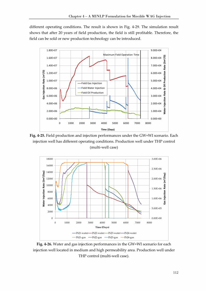
Chapter 4 – A MINLP Formulation for Miscible WAG Injection
112
different operating conditions. The result is shown in Fig. 4-29. The simulation result shows that after 20 years of field production, the field is still profitable. Therefore, the field can be sold or new production technology can be introduced.
Fig. 4-25. Field production and injection performances under the GW+WI scenario. Each
injection well has different operating conditions. Production well under THP control (multi-well case)
Fig. 4-26. Water and gas injection performances in the GW+WI scenario for each
injection well located in medium and high permeability area. Production well under THP control (multi-well case).
0.00E+00
1.00E+04
2.00E+04
3.00E+04
4.00E+04
5.00E+04
6.00E+04
7.00E+04
8.00E+04
9.00E+04
0.00E+00
2.00E+06
4.00E+06
6.00E+06
8.00E+06
1.00E+07
1.20E+07
1.40E+07
1.60E+07
1.80E+07
0 1000 2000 3000 4000 5000 6000 7000 8000
Wat
er In
ject
ion
Rate
& O
Il Pr
oduc
tion
Rate
(Sm
3 /D)
Gas I
njec
tion
Rate
(m3 /
D)
Time (Days)
Field Gas Injection
Field Water Injection
Field Oil Production
Maximum Field Operation Time
0.00E+00
5.00E+05
1.00E+06
1.50E+06
2.00E+06
2.50E+06
3.00E+06
0
2000
4000
6000
8000
10000
12000
14000
16000
18000
0 1000 2000 3000 4000 5000 6000 7000 8000
Gas I
njec
tion
Rate
(m3 /
Day)
Wat
er In
ject
ion
Rate
(Sm
3 /Da
y)
Time (Days)
INJ1-water INJ2-water INJ3-water INJ4-water
INJ1-gas INJ2-gas INJ3-gas INJ4-gas
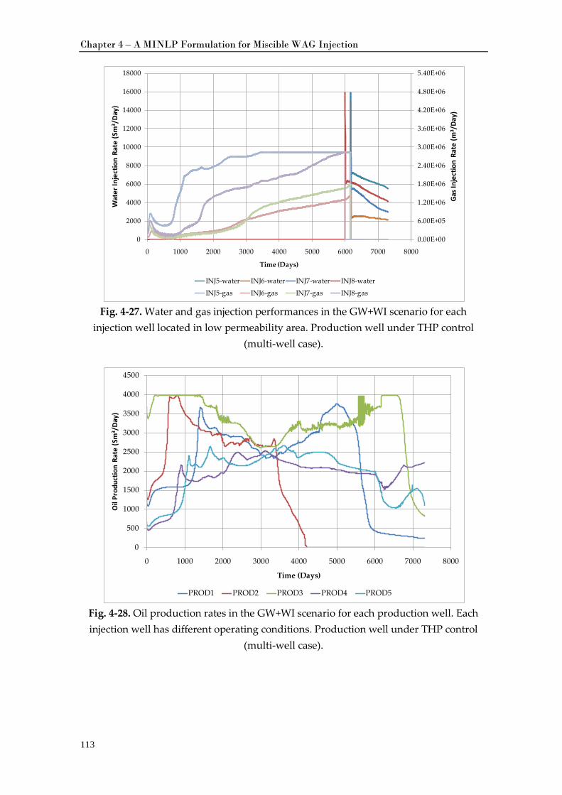
Chapter 4 – A MINLP Formulation for Miscible WAG Injection
113
Fig. 4-27. Water and gas injection performances in the GW+WI scenario for each
injection well located in low permeability area. Production well under THP control (multi-well case).
Fig. 4-28. Oil production rates in the GW+WI scenario for each production well. Each injection well has different operating conditions. Production well under THP control
(multi-well case).
0.00E+00
6.00E+05
1.20E+06
1.80E+06
2.40E+06
3.00E+06
3.60E+06
4.20E+06
4.80E+06
5.40E+06
0
2000
4000
6000
8000
10000
12000
14000
16000
18000
0 1000 2000 3000 4000 5000 6000 7000 8000
Gas I
njec
tion
Rate
(m3 /
Day)
Wat
er In
ject
ion
Rate
(Sm
3 /Da
y)
Time (Days)
INJ5-water INJ6-water INJ7-water INJ8-water
INJ5-gas INJ6-gas INJ7-gas INJ8-gas
0
500
1000
1500
2000
2500
3000
3500
4000
4500
0 1000 2000 3000 4000 5000 6000 7000 8000
Oil
Prod
uctio
n Ra
te (S
m3 /
Day)
Time (Days)
PROD1 PROD2 PROD3 PROD4 PROD5
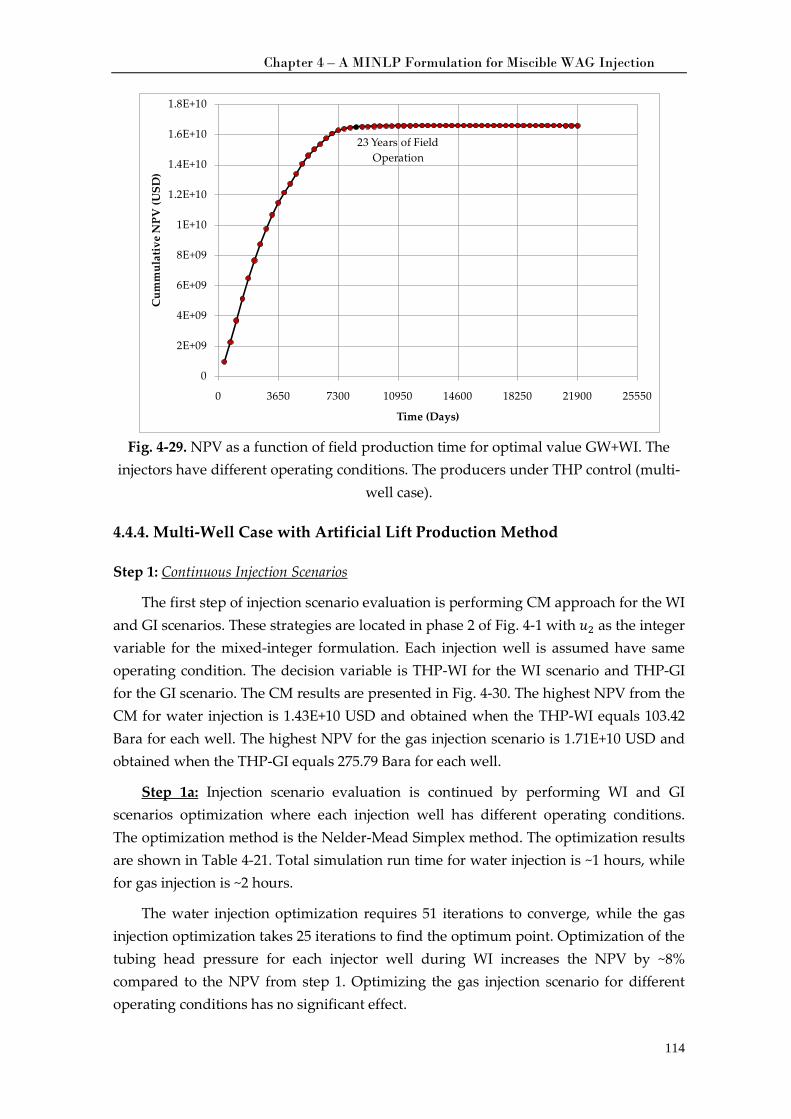
Chapter 4 – A MINLP Formulation for Miscible WAG Injection
114
Fig. 4-29. NPV as a function of field production time for optimal value GW+WI. The
injectors have different operating conditions. The producers under THP control (multi-well case).
4.4.4. Multi-Well Case with Artificial Lift Production Method
Step 1: Continuous Injection Scenarios
The first step of injection scenario evaluation is performing CM approach for the WI and GI scenarios. These strategies are located in phase 2 of
Fig. 4-1 with 𝑢2 as the integer variable for the mixed-integer formulation. Each injection well is assumed have same operating condition. The decision variable is THP-WI for the WI scenario and THP-GI for the GI scenario. The CM results are presented in Fig. 4-30. The highest NPV from the CM for water injection is 1.43E+10 USD and obtained when the THP-WI equals 103.42 Bara for each well. The highest NPV for the gas injection scenario is 1.71E+10 USD and obtained when the THP-GI equals 275.79 Bara for each well.
Step 1a:
Table 4-21
Injection scenario evaluation is continued by performing WI and GI scenarios optimization where each injection well has different operating conditions. The optimization method is the Nelder-Mead Simplex method. The optimization results are shown in . Total simulation run time for water injection is ~1 hours, while for gas injection is ~2 hours.
The water injection optimization requires 51 iterations to converge, while the gas injection optimization takes 25 iterations to find the optimum point. Optimization of the tubing head pressure for each injector well during WI increases the NPV by ~8% compared to the NPV from step 1. Optimizing the gas injection scenario for different operating conditions has no significant effect.
23 Years of Field Operation
0
2E+09
4E+09
6E+09
8E+09
1E+10
1.2E+10
1.4E+10
1.6E+10
1.8E+10
0 3650 7300 10950 14600 18250 21900 25550
Cum
mul
ativ
e N
PV (U
SD)
Time (Days)
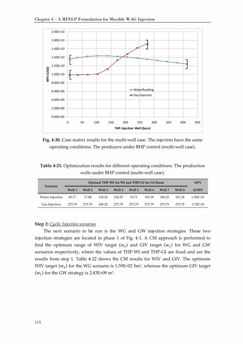
Chapter 4 – A MINLP Formulation for Miscible WAG Injection
115
Fig. 4-30. Case matrix results for the multi-well case. The injectors have the same
operating conditions. The producers under BHP control (multi-well case).
Table 4-21. Optimization results for different operating conditions. The production wells under BHP control (multi-well case).
Step 2: Cyclic Injection scenariosThe next scenario to be run is the WG and GW injection strategies. These two
injection strategies are located in phase 1 of
Fig. 4-1. A CM approach is performed to find the optimum range of WIV target (𝑤𝑤2) and GIV target (𝑤𝑤1) for WG and GW scenarios respectively, where the values of THP-WI and THP-GI are fixed and are the results from step 1. Table 4-22 shows the CM results for WIV and GIV. The optimum WIV target (𝑤𝑤2) for the WG scenario is 1.59E+02 Sm3, whereas the optimum GIV target (𝑤𝑤1) for the GW strategy is 2.83E+09 m3.
0.00E+00
2.00E+09
4.00E+09
6.00E+09
8.00E+09
1.00E+10
1.20E+10
1.40E+10
1.60E+10
1.80E+10
2.00E+10
0 50 100 150 200 250 300 350 400 450
NPV
(USD
)
THP Injection Well (bara)
WaterfloodingGas Injection
NPV
Well 1 Well 2 Well 3 Well 4 Well 5 Well 6 Well 7 Well 8 (USD)
Water Injection 60.77 17.88 130.26 234.55 53.71 195.39 186.25 101.34 1.56E+10
Gas Injection 275.79 275.79 248.22 275.79 275.79 275.79 275.79 275.79 1.72E+10
ScenarioOptimal THP-WI for WI and THP-GI for GI (bara)
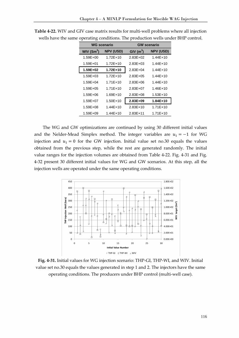
Chapter 4 – A MINLP Formulation for Miscible WAG Injection
116
Table 4-22. WIV and GIV case matrix results for multi-well problems where all injection wells have the same operating conditions. The production wells under BHP control.
The WG and GW optimizations are continued by using 30 different initial values and the Nelder-Mead Simplex method. The integer variables are 𝑢1 = −1 for WG injection and 𝑢1 = 0 for the GW injection. Initial value set no.30 equals the values obtained from the previous step, while the rest are generated randomly. The initial value ranges for the injection volumes are obtained from Table 4-22. Fig. 4-31 and Fig. 4-32 present 30 different initial values for WG and GW scenarios. At this step, all the injection wells are operated under the same operating conditions.
Fig. 4-31. Initial values for WG injection scenario: THP-GI, THP-WI, and WIV. Initial
value set no.30 equals the values generated in step 1 and 2. The injectors have the same operating conditions. The producers under BHP control (multi-well case).
WIV (Sm3) NPV (USD) GIV (m3) NPV (USD)1.59E+00 1.72E+10 2.83E+02 1.44E+10
1.59E+01 1.72E+10 2.83E+03 1.44E+10
1.59E+02 1.72E+10 2.83E+04 1.44E+10
1.59E+03 1.72E+10 2.83E+05 1.44E+10
1.59E+04 1.71E+10 2.83E+06 1.44E+10
1.59E+05 1.71E+10 2.83E+07 1.46E+10
1.59E+06 1.69E+10 2.83E+08 1.53E+10
1.59E+07 1.50E+10 2.83E+09 1.84E+101.59E+08 1.44E+10 2.83E+10 1.71E+10
1.59E+09 1.44E+10 2.83E+11 1.71E+10
WG scenario GW scenario
0.00E+00
2.00E+01
4.00E+01
6.00E+01
8.00E+01
1.00E+02
1.20E+02
1.40E+02
1.60E+02
1.80E+02
0
50
100
150
200
250
300
350
400
450
0 5 10 15 20 25 30
WIV
tar
get (
Sm3 )
THP
Inje
ctio
n W
ell (
bara
)
Initial Value Number
THP-GI THP-WI WIV
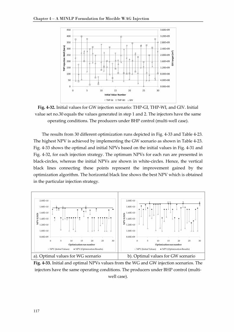
Chapter 4 – A MINLP Formulation for Miscible WAG Injection
117
Fig. 4-32. Initial values for GW injection scenario: THP-GI, THP-WI, and GIV. Initial
value set no.30 equals the values generated in step 1 and 2. The injectors have the same operating conditions. The producers under BHP control (multi-well case).
The results from 30 different optimization runs depicted in Fig. 4-33 and Table 4-23.
The highest NPV is achieved by implementing the GW scenario as shown in Table 4-23. Fig. 4-33 shows the optimal and initial NPVs based on the initial values in Fig. 4-31 and Fig. 4-32, for each injection strategy. The optimum NPVs for each run are presented in black-circles, whereas the initial NPVs are shown in white-circles. Hence, the vertical black lines connecting these points represent the improvement gained by the optimization algorithm. The horizontal black line shows the best NPV which is obtained in the particular injection strategy.
a). Optimal values for WG scenario b). Optimal values for GW scenario Fig. 4-33. Initial and optimal NPVs values from the WG and GW injection scenarios. The injectors have the same operating conditions. The producers under BHP control (multi-
well case).
0.00E+00
4.00E+08
8.00E+08
1.20E+09
1.60E+09
2.00E+09
2.40E+09
2.80E+09
3.20E+09
3.60E+09
0
50
100
150
200
250
300
350
400
450
0 5 10 15 20 25 30
GIV
targ
et (m
3 )
THP
Inje
ctio
n W
ell (
bara
)
Initial Value Number
THP-GI THP-WI GIV
8.00E+09
1.00E+10
1.20E+10
1.40E+10
1.60E+10
1.80E+10
2.00E+10
0 5 10 15 20 25 30
NPV
(USD
)
Optimization run number
NPV (Initial Values) NPV (Optimization Results)
1 23
8.00E+09
1.00E+10
1.20E+10
1.40E+10
1.60E+10
1.80E+10
2.00E+10
0 5 10 15 20 25 30
NPV
(USD
)
Optimization run number
NPV (Initial Values) NPV (Optimization Results)
51 2 3 4
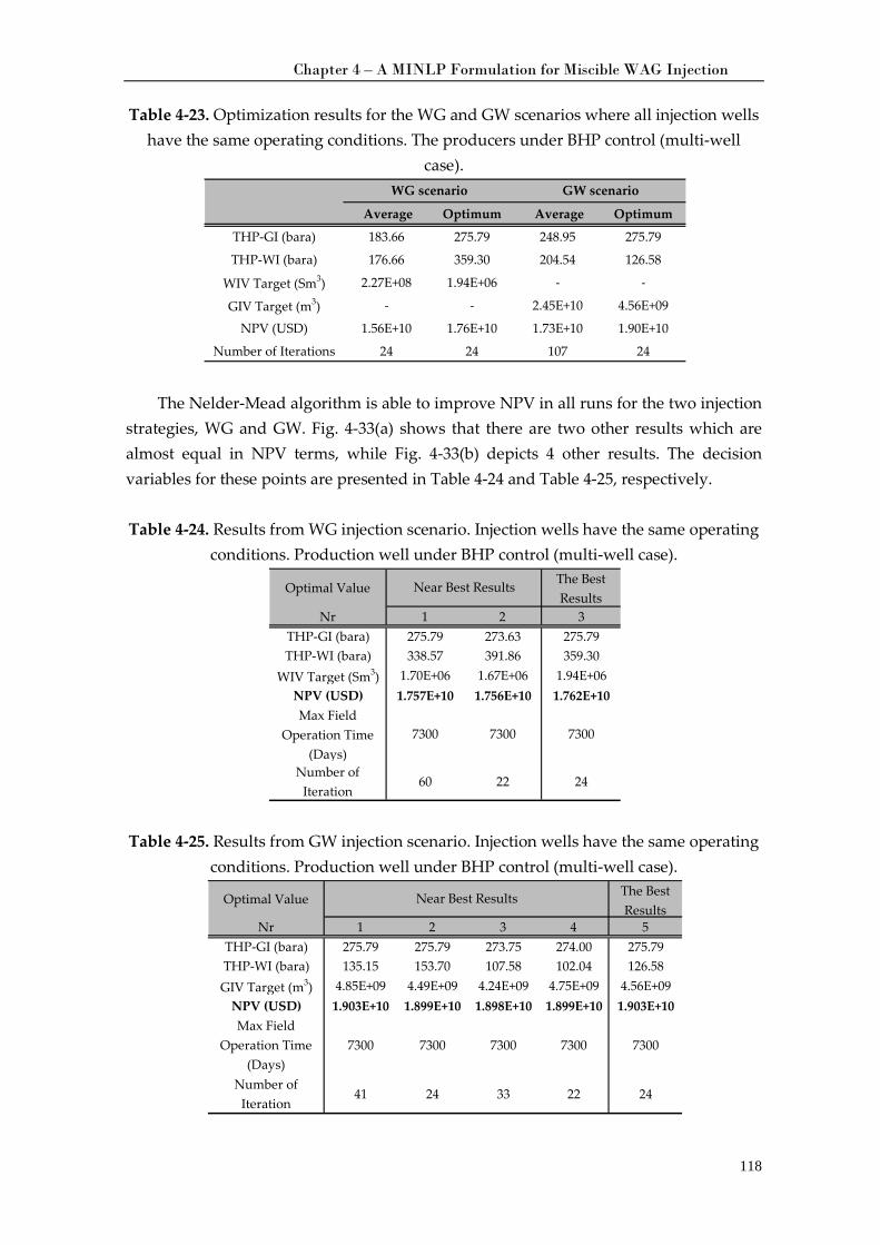
Chapter 4 – A MINLP Formulation for Miscible WAG Injection
118
Table 4-23. Optimization results for the WG and GW scenarios where all injection wells have the same operating conditions. The producers under BHP control (multi-well
case).
The Nelder-Mead algorithm is able to improve NPV in all runs for the two injection
strategies, WG and GW. Fig. 4-33(a) shows that there are two other results which are almost equal in NPV terms, while Fig. 4-33(b) depicts 4 other results. The decision variables for these points are presented in Table 4-24 and Table 4-25, respectively.
Table 4-24. Results from WG injection scenario. Injection wells have the same operating
conditions. Production well under BHP control (multi-well case).
Table 4-25. Results from GW injection scenario. Injection wells have the same operating conditions. Production well under BHP control (multi-well case).
Average Optimum Average Optimum
THP-GI (bara) 183.66 275.79 248.95 275.79
THP-WI (bara) 176.66 359.30 204.54 126.58
WIV Target (Sm3) 2.27E+08 1.94E+06 - -
GIV Target (m3) - - 2.45E+10 4.56E+09
NPV (USD) 1.56E+10 1.76E+10 1.73E+10 1.90E+10
Number of Iterations 24 24 107 24
WG scenario GW scenario
Optimal ValueThe Best Results
Nr 1 2 3THP-GI (bara) 275.79 273.63 275.79THP-WI (bara) 338.57 391.86 359.30
WIV Target (Sm3) 1.70E+06 1.67E+06 1.94E+06NPV (USD) 1.757E+10 1.756E+10 1.762E+10Max Field
Operation Time (Days)
7300 7300 7300
Number of Iteration
60 22 24
Near Best Results
Optimal Value The Best Results
Nr 1 2 3 4 5THP-GI (bara) 275.79 275.79 273.75 274.00 275.79THP-WI (bara) 135.15 153.70 107.58 102.04 126.58GIV Target (m3) 4.85E+09 4.49E+09 4.24E+09 4.75E+09 4.56E+09
NPV (USD) 1.903E+10 1.899E+10 1.898E+10 1.899E+10 1.903E+10Max Field
Operation Time (Days)
7300 7300 7300 7300 7300
Number of Iteration
41 24 33 22 24
Near Best Results
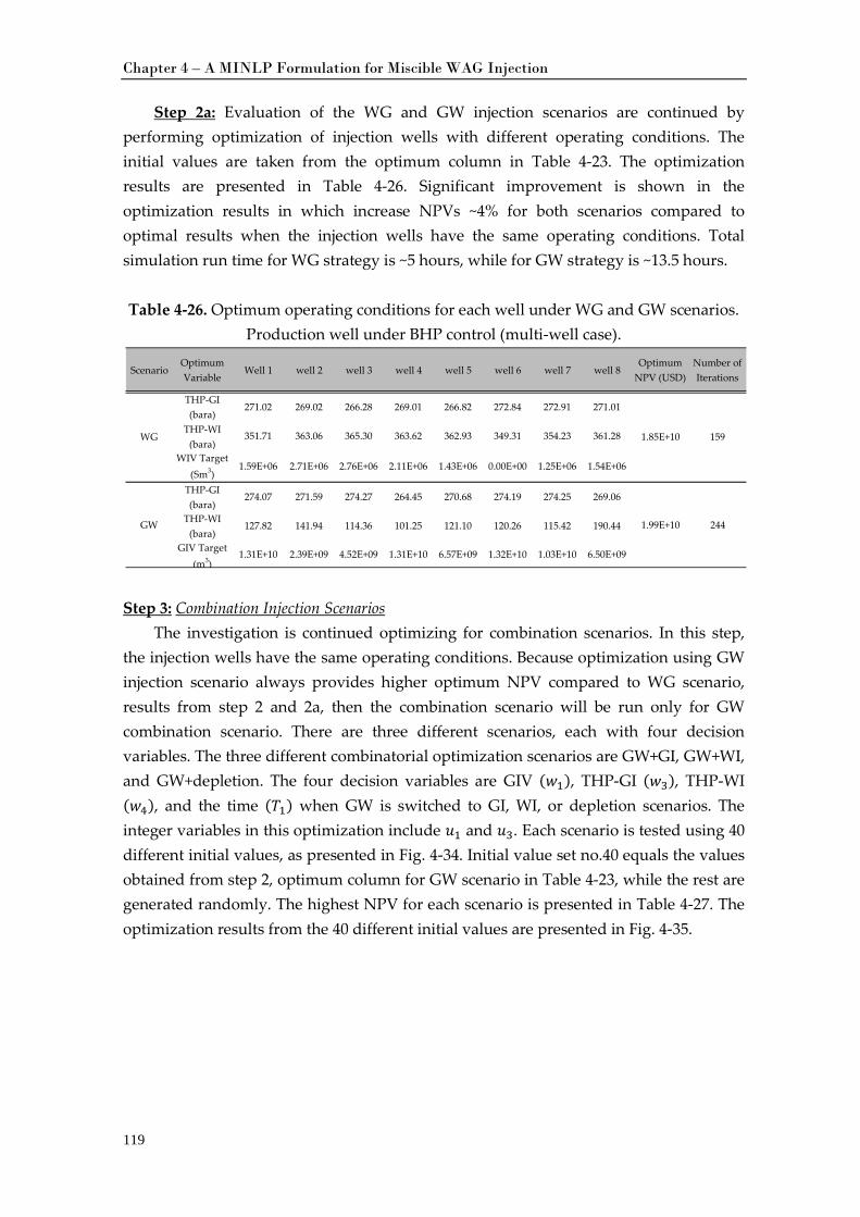
Chapter 4 – A MINLP Formulation for Miscible WAG Injection
119
Step 2a:
Table 4-23
Evaluation of the WG and GW injection scenarios are continued by performing optimization of injection wells with different operating conditions. The initial values are taken from the optimum column in . The optimization results are presented in Table 4-26. Significant improvement is shown in the optimization results in which increase NPVs ~4% for both scenarios compared to optimal results when the injection wells have the same operating conditions. Total simulation run time for WG strategy is ~5 hours, while for GW strategy is ~13.5 hours.
Table 4-26. Optimum operating conditions for each well under WG and GW scenarios.
Production well under BHP control (multi-well case).
Step 3: The investigation is continued optimizing for combination scenarios. In this step,
the injection wells have the same operating conditions. Because optimization using GW injection scenario always provides higher optimum NPV compared to WG scenario, results from step 2 and 2a, then the combination scenario will be run only for GW combination scenario. There are three different scenarios, each with four decision variables. The three different combinatorial optimization scenarios are GW+GI, GW+WI, and GW+depletion. The four decision variables are GIV (𝑤𝑤1), THP-GI (𝑤𝑤3), THP-WI (𝑤𝑤4), and the time (𝑇𝑇1) when GW is switched to GI, WI, or depletion scenarios. The integer variables in this optimization include 𝑢1 and 𝑢3. Each scenario is tested using 40 different initial values, as presented in
Combination Injection Scenarios
Fig. 4-34. Initial value set no.40 equals the values obtained from step 2, optimum column for GW scenario in Table 4-23, while the rest are generated randomly. The highest NPV for each scenario is presented in Table 4-27. The optimization results from the 40 different initial values are presented in Fig. 4-35.
ScenarioOptimum Variable
Well 1 well 2 well 3 well 4 well 5 well 6 well 7 well 8Optimum
NPV (USD)Number of Iterations
THP-GI (bara)
271.02 269.02 266.28 269.01 266.82 272.84 272.91 271.01
THP-WI (bara)
351.71 363.06 365.30 363.62 362.93 349.31 354.23 361.28
WIV Target (Sm3)
1.59E+06 2.71E+06 2.76E+06 2.11E+06 1.43E+06 0.00E+00 1.25E+06 1.54E+06
THP-GI (bara)
274.07 271.59 274.27 264.45 270.68 274.19 274.25 269.06
THP-WI (bara)
127.82 141.94 114.36 101.25 121.10 120.26 115.42 190.44
GIV Target (m3)
1.31E+10 2.39E+09 4.52E+09 1.31E+10 6.57E+09 1.32E+10 1.03E+10 6.50E+09
WG 1.85E+10 159
GW 1.99E+10 244
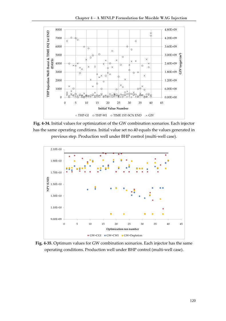
Chapter 4 – A MINLP Formulation for Miscible WAG Injection
120
Fig. 4-34. Initial values for optimization of the GW combination scenarios. Each injector has the same operating conditions. Initial value set no.40 equals the values generated in
previous step. Production well under BHP control (multi-well case).
Fig. 4-35. Optimum values for GW combination scenarios. Each injector has the same
operating conditions. Production well under BHP control (multi-well case).
0.00E+00
6.00E+08
1.20E+09
1.80E+09
2.40E+09
3.00E+09
3.60E+09
4.20E+09
4.80E+09
0
1000
2000
3000
4000
5000
6000
7000
8000
0 5 10 15 20 25 30 35 40 45
GIV
targ
et (m
3 )
THP
Inje
ctio
n W
ell (
bara
) & T
IME
INJ 1
st E
ND
(D
AYS)
Initial Value Number
THP-GI THP-WI TIME 1ST-SCN END GIV
9.00E+09
1.10E+10
1.30E+10
1.50E+10
1.70E+10
1.90E+10
2.10E+10
0 5 10 15 20 25 30 35 40 45
NPV
(USD
)
Optimization run number
GW+CGI GW+CWI GW+Depletion
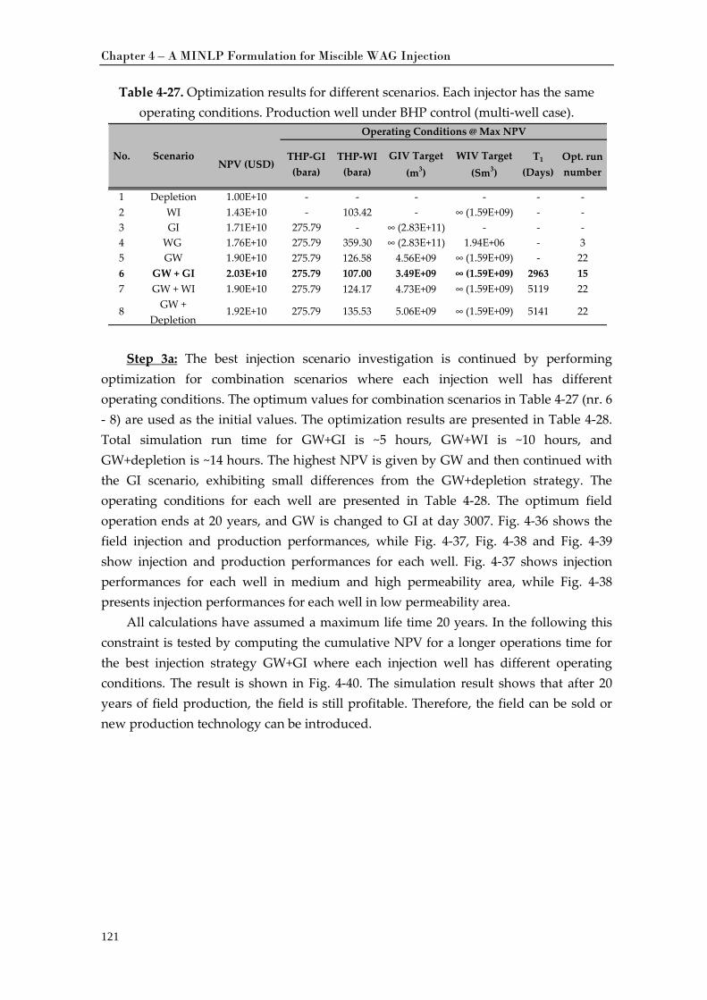
Chapter 4 – A MINLP Formulation for Miscible WAG Injection
121
Table 4-27. Optimization results for different scenarios. Each injector has the same operating conditions. Production well under BHP control (multi-well case).
Step 3a:
Table 4-27
The best injection scenario investigation is continued by performing optimization for combination scenarios where each injection well has different operating conditions. The optimum values for combination scenarios in (nr. 6 - 8) are used as the initial values. The optimization results are presented in Table 4-28. Total simulation run time for GW+GI is ~5 hours, GW+WI is ~10 hours, and GW+depletion is ~14 hours. The highest NPV is given by GW and then continued with the GI scenario, exhibiting small differences from the GW+depletion strategy. The operating conditions for each well are presented in Table 4-28. The optimum field operation ends at 20 years, and GW is changed to GI at day 3007. Fig. 4-36 shows the field injection and production performances, while Fig. 4-37, Fig. 4-38 and Fig. 4-39 show injection and production performances for each well. Fig. 4-37 shows injection performances for each well in medium and high permeability area, while Fig. 4-38 presents injection performances for each well in low permeability area.
All calculations have assumed a maximum life time 20 years. In the following this constraint is tested by computing the cumulative NPV for a longer operations time for the best injection strategy GW+GI where each injection well has different operating conditions. The result is shown in Fig. 4-40. The simulation result shows that after 20 years of field production, the field is still profitable. Therefore, the field can be sold or new production technology can be introduced.
NPV (USD)THP-GI (bara)
THP-WI (bara)
GIV Target (m3)
WIV Target (Sm3)
T1
(Days)Opt. run number
1 Depletion 1.00E+10 - - - - - -2 WI 1.43E+10 - 103.42 - ∞ (1.59E+09) - -3 GI 1.71E+10 275.79 - ∞ (2.83E+11) - - -4 WG 1.76E+10 275.79 359.30 ∞ (2.83E+11) 1.94E+06 - 35 GW 1.90E+10 275.79 126.58 4.56E+09 ∞ (1.59E+09) - 226 GW + GI 2.03E+10 275.79 107.00 3.49E+09 ∞ (1.59E+09) 2963 157 GW + WI 1.90E+10 275.79 124.17 4.73E+09 ∞ (1.59E+09) 5119 22
8 GW + Depletion
1.92E+10 275.79 135.53 5.06E+09 ∞ (1.59E+09) 5141 22
Operating Conditions @ Max NPV
No. Scenario
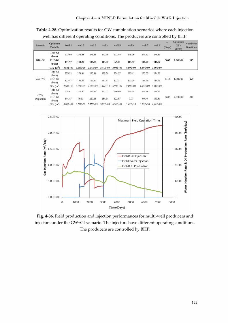
Chapter 4 – A MINLP Formulation for Miscible WAG Injection
122
Table 4-28. Optimization results for GW combination scenarios where each injection well has different operating conditions. The producers are controlled by BHP.
Fig. 4-36. Field production and injection performances for multi-well producers and
injectors under the GW+GI scenario. The injectors have different operating conditions. The producers are controlled by BHP.
ScenarioOptimum Variable
Well 1 well 2 well 3 well 4 well 5 well 6 well 7 well 8T1
(Days)
Optimum NPV
(USD)
Number of Iterations
THP-GI (bara)
273.96 272.48 273.65 272.48 272.48 275.26 274.92 274.63
THP-WI (bara)
111.97 111.97 114.78 111.97 67.30 111.97 111.97 111.97
GIV (m3) 3.53E+09 3.69E+09 3.34E+09 3.44E+09 3.90E+09 6.89E+09 6.89E+09 3.99E+09THP-GI (bara)
275.32 274.84 275.18 275.28 274.37 275.41 275.55 274.73
THP-WI (bara)
123.47 133.33 123.17 111.51 122.71 123.29 116.99 114.96
GIV (m3) 2.58E+10 3.55E+09 4.97E+09 1.66E+10 5.99E+09 7.09E+09 6.75E+09 5.08E+09THP-GI (bara)
274.61 272.50 273.16 272.02 246.89 275.34 275.58 274.51
THP-WI (bara)
144.47 79.53 220.18 284.54 122.87 0.07 90.36 133.81
GIV (m3) 8.81E+09 6.30E+09 5.77E+09 3.92E+09 6.31E+09 1.62E+10 1.29E+10 6.44E+09
GW+ Depletion
5637 2.03E+10 310
GW+GI 3007 2.04E+10 115
GW+WI 5113 1.98E+10 229
0
12000
24000
36000
48000
60000
0.00E+00
5.00E+06
1.00E+07
1.50E+07
2.00E+07
2.50E+07
0 1000 2000 3000 4000 5000 6000 7000 8000
Wat
er In
ject
ion
Rate
& O
il Pr
oduc
tion
Rate
(Sm
3 /da
y)
Gas I
njec
tion
Rate
(m3 /
day)
Time (Days)
Field Gas Injection
Field Water Injection
Field Oil Production
Maximum Field Operation Time
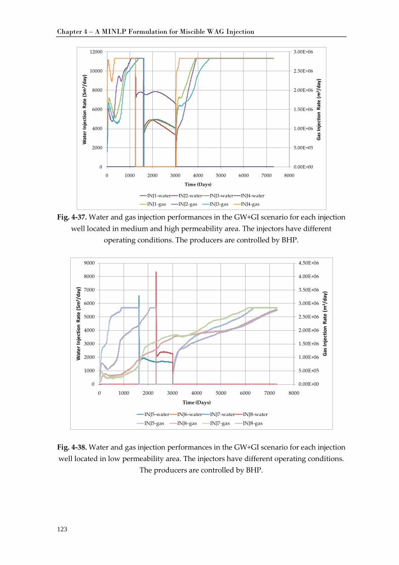
Chapter 4 – A MINLP Formulation for Miscible WAG Injection
123
Fig. 4-37. Water and gas injection performances in the GW+GI scenario for each injection
well located in medium and high permeability area. The injectors have different operating conditions. The producers are controlled by BHP.
Fig. 4-38. Water and gas injection performances in the GW+GI scenario for each injection well located in low permeability area. The injectors have different operating conditions.
The producers are controlled by BHP.
0.00E+00
5.00E+05
1.00E+06
1.50E+06
2.00E+06
2.50E+06
3.00E+06
0
2000
4000
6000
8000
10000
12000
0 1000 2000 3000 4000 5000 6000 7000 8000
Gas I
njec
tion
Rate
(m3 /
day)
Wat
er In
ject
ion
Rate
(Sm
3 /da
y)
Time (Days)
INJ1-water INJ2-water INJ3-water INJ4-water
INJ1-gas INJ2-gas INJ3-gas INJ4-gas
0.00E+00
5.00E+05
1.00E+06
1.50E+06
2.00E+06
2.50E+06
3.00E+06
3.50E+06
4.00E+06
4.50E+06
0
1000
2000
3000
4000
5000
6000
7000
8000
9000
0 1000 2000 3000 4000 5000 6000 7000 8000
Gas I
njec
tion
Rate
(m3 /
day)
Wat
er In
ject
ion
Rate
(Sm
3 /da
y)
Time (Days)
INJ5-water INJ6-water INJ7-water INJ8-water
INJ5-gas INJ6-gas INJ7-gas INJ8-gas
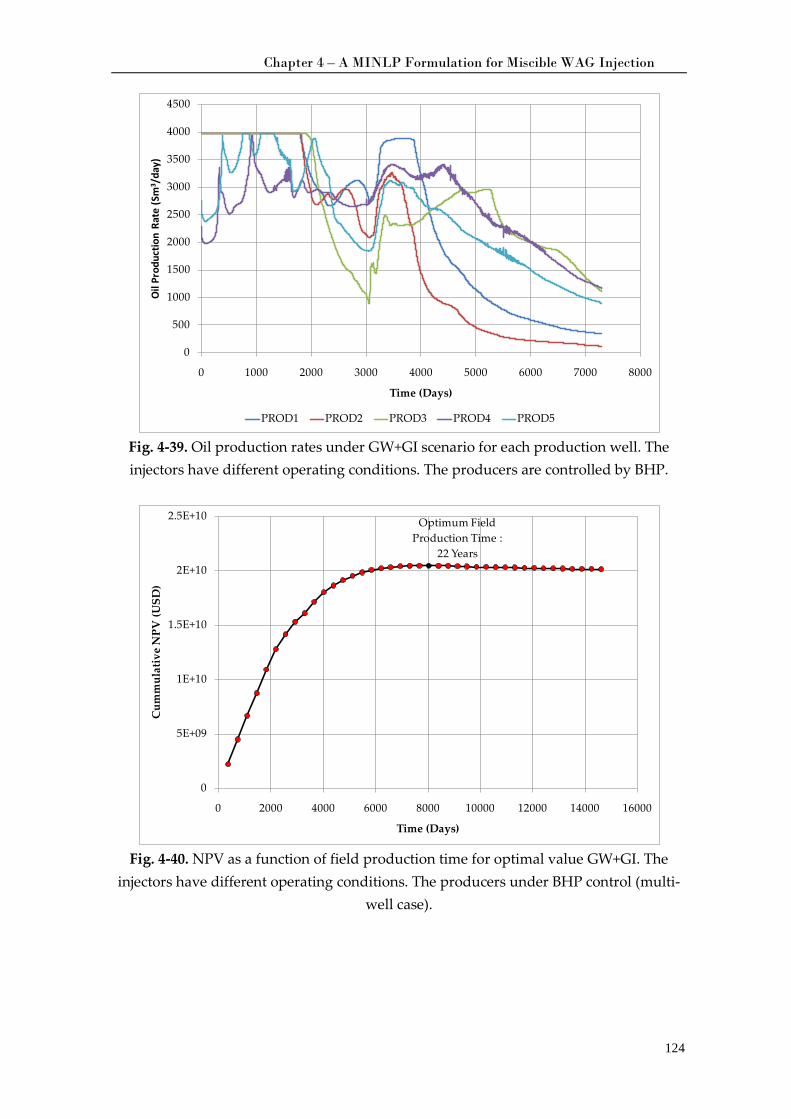
Chapter 4 – A MINLP Formulation for Miscible WAG Injection
124
Fig. 4-39. Oil production rates under GW+GI scenario for each production well. The injectors have different operating conditions. The producers are controlled by BHP.
Fig. 4-40. NPV as a function of field production time for optimal value GW+GI. The
injectors have different operating conditions. The producers under BHP control (multi-well case).
0
500
1000
1500
2000
2500
3000
3500
4000
4500
0 1000 2000 3000 4000 5000 6000 7000 8000
Oil
Prod
uctio
n Ra
te (S
m3 /
day)
Time (Days)
PROD1 PROD2 PROD3 PROD4 PROD5
Optimum Field Production Time :
22 Years
0
5E+09
1E+10
1.5E+10
2E+10
2.5E+10
0 2000 4000 6000 8000 10000 12000 14000 16000
Cum
mul
ativ
e N
PV (U
SD)
Time (Days)
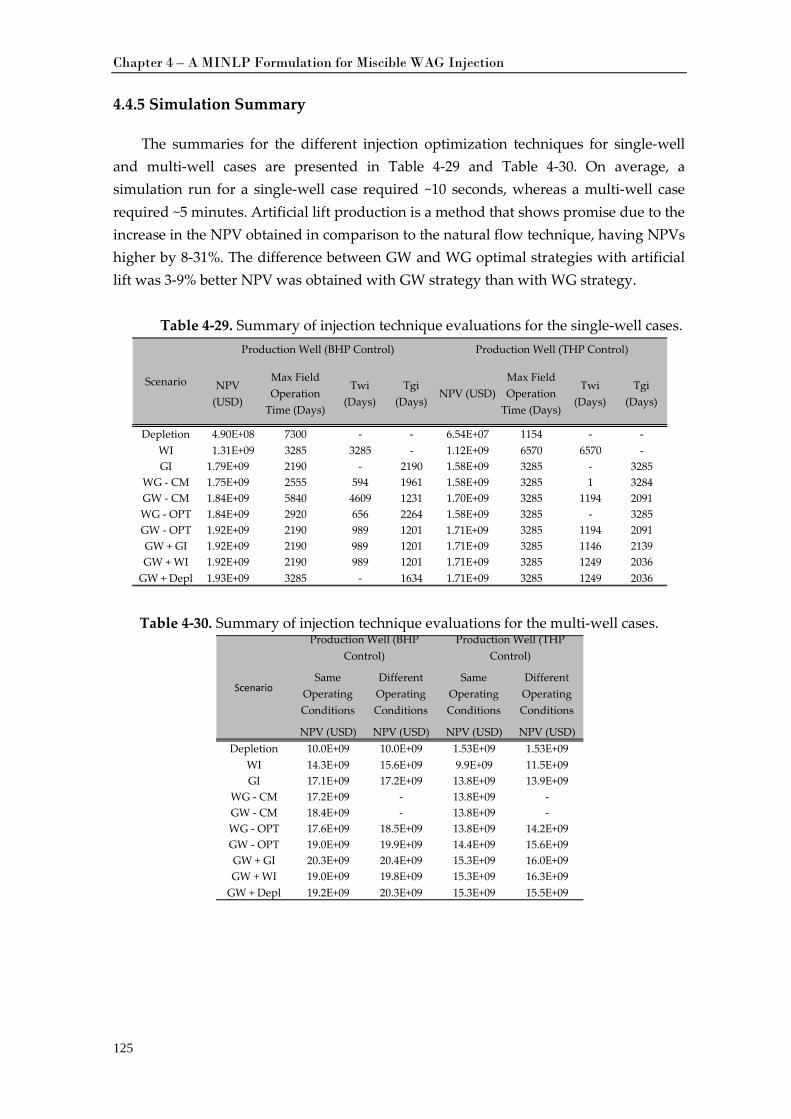
Chapter 4 – A MINLP Formulation for Miscible WAG Injection
125
4.4.5 Simulation Summary
The summaries for the different injection optimization techniques for single-well and multi-well cases are presented in Table 4-29 and Table 4-30. On average, a simulation run for a single-well case required ~10 seconds, whereas a multi-well case required ~5 minutes. Artificial lift production is a method that shows promise due to the increase in the NPV obtained in comparison to the natural flow technique, having NPVs higher by 8-31%. The difference between GW and WG optimal strategies with artificial lift was 3-9% better NPV was obtained with GW strategy than with WG strategy.
Table 4-29. Summary of injection technique evaluations for the single-well cases.
Table 4-30. Summary of injection technique evaluations for the multi-well cases.
NPV (USD)
Max Field Operation
Time (Days)
Twi (Days)
Tgi (Days)
NPV (USD)Max Field Operation
Time (Days)
Twi (Days)
Tgi (Days)
Depletion 4.90E+08 7300 - - 6.54E+07 1154 - -WI 1.31E+09 3285 3285 - 1.12E+09 6570 6570 -GI 1.79E+09 2190 - 2190 1.58E+09 3285 - 3285
WG - CM 1.75E+09 2555 594 1961 1.58E+09 3285 1 3284GW - CM 1.84E+09 5840 4609 1231 1.70E+09 3285 1194 2091WG - OPT 1.84E+09 2920 656 2264 1.58E+09 3285 - 3285GW - OPT 1.92E+09 2190 989 1201 1.71E+09 3285 1194 2091GW + GI 1.92E+09 2190 989 1201 1.71E+09 3285 1146 2139GW + WI 1.92E+09 2190 989 1201 1.71E+09 3285 1249 2036
GW + Depl 1.93E+09 3285 - 1634 1.71E+09 3285 1249 2036
Scenario
Production Well (BHP Control) Production Well (THP Control)
Same Operating Conditions
Different Operating Conditions
Same Operating Conditions
Different Operating Conditions
NPV (USD) NPV (USD) NPV (USD) NPV (USD)Depletion 10.0E+09 10.0E+09 1.53E+09 1.53E+09
WI 14.3E+09 15.6E+09 9.9E+09 11.5E+09GI 17.1E+09 17.2E+09 13.8E+09 13.9E+09
WG - CM 17.2E+09 - 13.8E+09 -GW - CM 18.4E+09 - 13.8E+09 -WG - OPT 17.6E+09 18.5E+09 13.8E+09 14.2E+09GW - OPT 19.0E+09 19.9E+09 14.4E+09 15.6E+09GW + GI 20.3E+09 20.4E+09 15.3E+09 16.0E+09GW + WI 19.0E+09 19.8E+09 15.3E+09 16.3E+09
GW + Depl 19.2E+09 20.3E+09 15.3E+09 15.5E+09
Scenario
Production Well (BHP Control)
Production Well (THP Control)
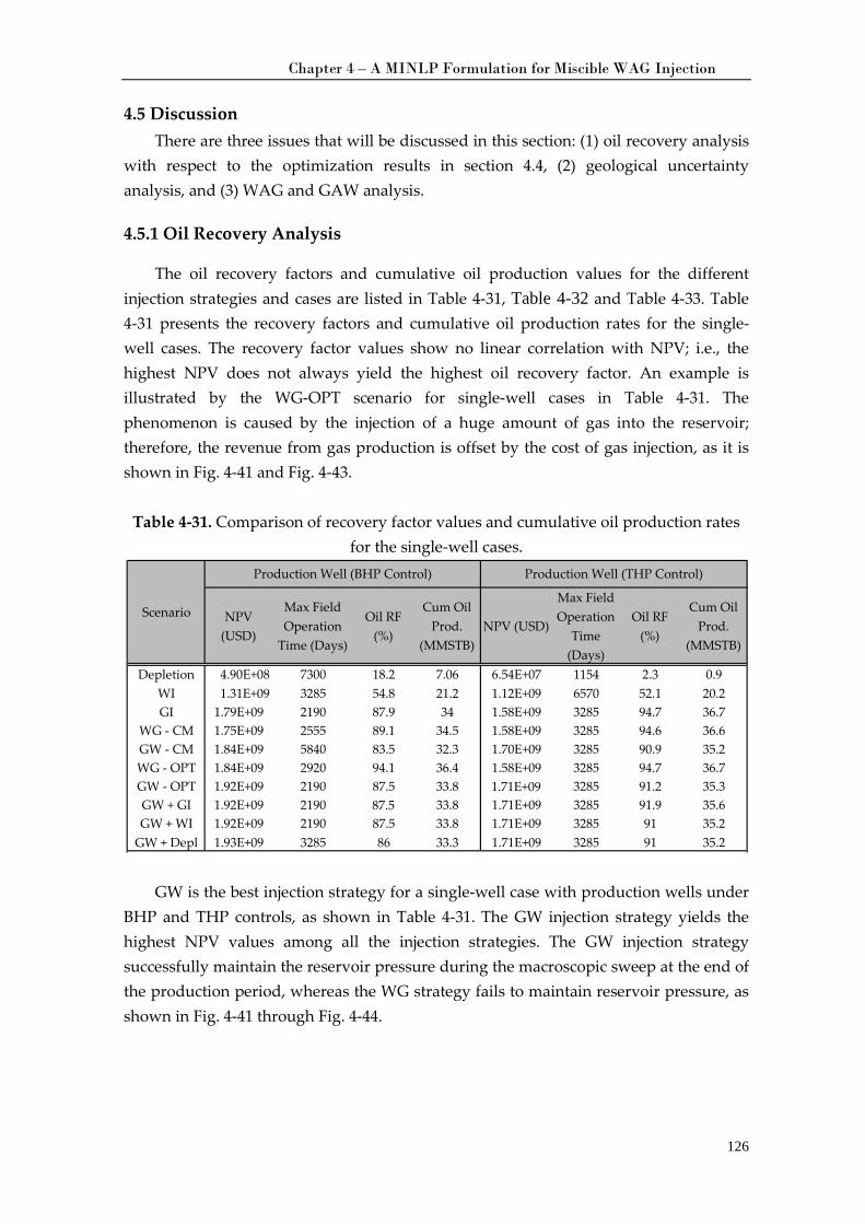
Chapter 4 – A MINLP Formulation for Miscible WAG Injection
126
4.5 Discussion There are three issues that will be discussed in this section: (1) oil recovery analysis
with respect to the optimization results in section 4.4, (2) geological uncertainty analysis, and (3) WAG and GAW analysis.
4.5.1 Oil Recovery Analysis
The oil recovery factors and cumulative oil production values for the different injection strategies and cases are listed in Table 4-31, Table 4-32 and Table 4-33. Table 4-31 presents the recovery factors and cumulative oil production rates for the single-well cases. The recovery factor values show no linear correlation with NPV; i.e., the highest NPV does not always yield the highest oil recovery factor. An example is illustrated by the WG-OPT scenario for single-well cases in Table 4-31. The phenomenon is caused by the injection of a huge amount of gas into the reservoir; therefore, the revenue from gas production is offset by the cost of gas injection, as it is shown in Fig. 4-41 and Fig. 4-43.
Table 4-31. Comparison of recovery factor values and cumulative oil production rates
for the single-well cases.
GW is the best injection strategy for a single-well case with production wells under BHP and THP controls, as shown in Table 4-31. The GW injection strategy yields the highest NPV values among all the injection strategies. The GW injection strategy successfully maintain the reservoir pressure during the macroscopic sweep at the end of the production period, whereas the WG strategy fails to maintain reservoir pressure, as shown in Fig. 4-41 through Fig. 4-44.
NPV (USD)
Max Field Operation
Time (Days)
Oil RF (%)
Cum Oil Prod.
(MMSTB)NPV (USD)
Max Field Operation
Time (Days)
Oil RF (%)
Cum Oil Prod.
(MMSTB)
Depletion 4.90E+08 7300 18.2 7.06 6.54E+07 1154 2.3 0.9WI 1.31E+09 3285 54.8 21.2 1.12E+09 6570 52.1 20.2GI 1.79E+09 2190 87.9 34 1.58E+09 3285 94.7 36.7
WG - CM 1.75E+09 2555 89.1 34.5 1.58E+09 3285 94.6 36.6GW - CM 1.84E+09 5840 83.5 32.3 1.70E+09 3285 90.9 35.2WG - OPT 1.84E+09 2920 94.1 36.4 1.58E+09 3285 94.7 36.7GW - OPT 1.92E+09 2190 87.5 33.8 1.71E+09 3285 91.2 35.3GW + GI 1.92E+09 2190 87.5 33.8 1.71E+09 3285 91.9 35.6GW + WI 1.92E+09 2190 87.5 33.8 1.71E+09 3285 91 35.2
GW + Depl 1.93E+09 3285 86 33.3 1.71E+09 3285 91 35.2
Scenario
Production Well (BHP Control) Production Well (THP Control)
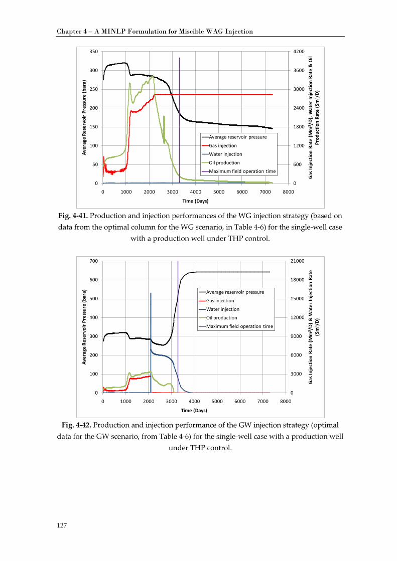
Chapter 4 – A MINLP Formulation for Miscible WAG Injection
127
Fig. 4-41. Production and injection performances of the WG injection strategy (based on data from the optimal column for the WG scenario, in Table 4-6) for the single-well case
with a production well under THP control.
Fig. 4-42. Production and injection performance of the GW injection strategy (optimal
data for the GW scenario, from Table 4-6) for the single-well case with a production well under THP control.
0
600
1200
1800
2400
3000
3600
4200
0
50
100
150
200
250
300
350
0 1000 2000 3000 4000 5000 6000 7000 8000
Gas I
njec
tion
Rate
(Mm
3 /D)
, Wat
er In
ject
ion
Rate
& O
il Pr
oduc
tion
Rate
(Sm
3 /D)
Aver
age
Rese
rvoi
r Pre
ssur
e (b
ara)
Time (Days)
Average reservoir pressure
Gas injection
Water injection
Oil production
Maximum field operation time
0
3000
6000
9000
12000
15000
18000
21000
0
100
200
300
400
500
600
700
0 1000 2000 3000 4000 5000 6000 7000 8000
Gas I
njec
tion
Rate
(Mm
3 /D)
& W
ater
Inje
ctio
n Ra
te
(Sm
3 /D)
Aver
age
Rese
rvoi
r Pre
ssur
e (b
ara)
Time (Days)
Average reservoir pressure
Gas injection
Water injection
Oil production
Maximum field operation time
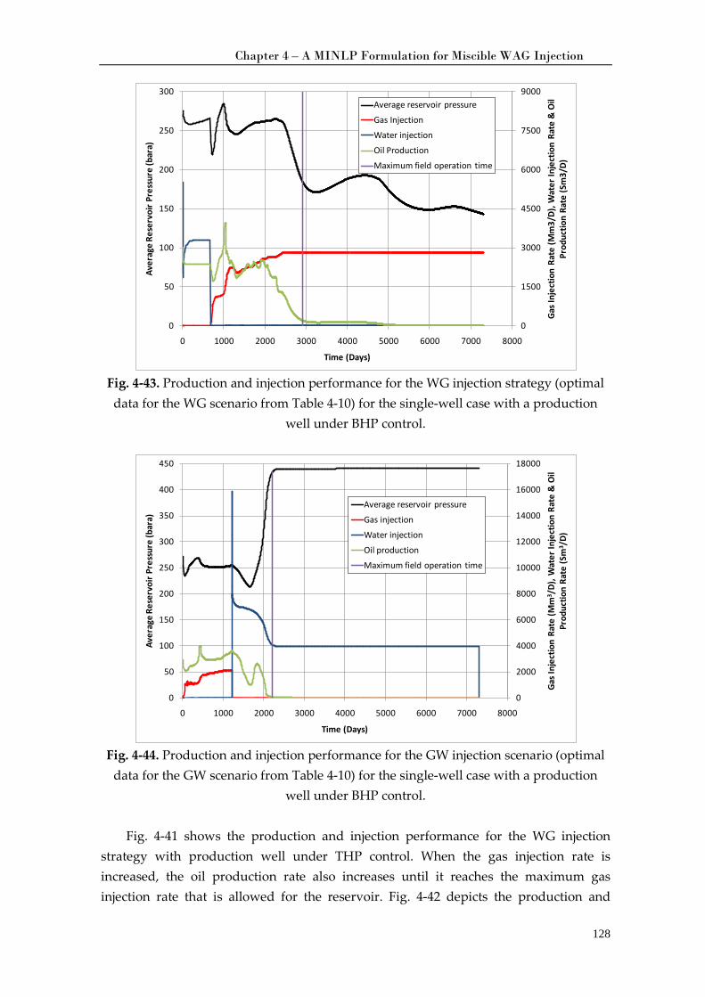
Chapter 4 – A MINLP Formulation for Miscible WAG Injection
128
Fig. 4-43. Production and injection performance for the WG injection strategy (optimal data for the WG scenario from Table 4-10) for the single-well case with a production
well under BHP control.
Fig. 4-44. Production and injection performance for the GW injection scenario (optimal
data for the GW scenario from Table 4-10) for the single-well case with a production well under BHP control.
Fig. 4-41 shows the production and injection performance for the WG injection
strategy with production well under THP control. When the gas injection rate is increased, the oil production rate also increases until it reaches the maximum gas injection rate that is allowed for the reservoir. Fig. 4-42 depicts the production and
0
1500
3000
4500
6000
7500
9000
0
50
100
150
200
250
300
0 1000 2000 3000 4000 5000 6000 7000 8000
Gas I
njec
tion
Rate
(Mm
3/D)
, Wat
er In
ject
ion
Rate
& O
il Pr
oduc
tion
Rate
(Sm
3/D)
Aver
age
Rese
rvoi
r Pre
ssur
e (b
ara)
Time (Days)
Average reservoir pressure
Gas Injection
Water injection
Oil Production
Maximum field operation time
0
2000
4000
6000
8000
10000
12000
14000
16000
18000
0
50
100
150
200
250
300
350
400
450
0 1000 2000 3000 4000 5000 6000 7000 8000
Gas I
njec
tion
Rate
(Mm
3 /D)
, Wat
er In
ject
ion
Rate
& O
il Pr
oduc
tion
Rate
(Sm
3 /D)
Aver
age
Rese
rvoi
r Pre
ssur
e (b
ara)
Time (Days)
Average reservoir pressure
Gas injection
Water injection
Oil production
Maximum field operation time
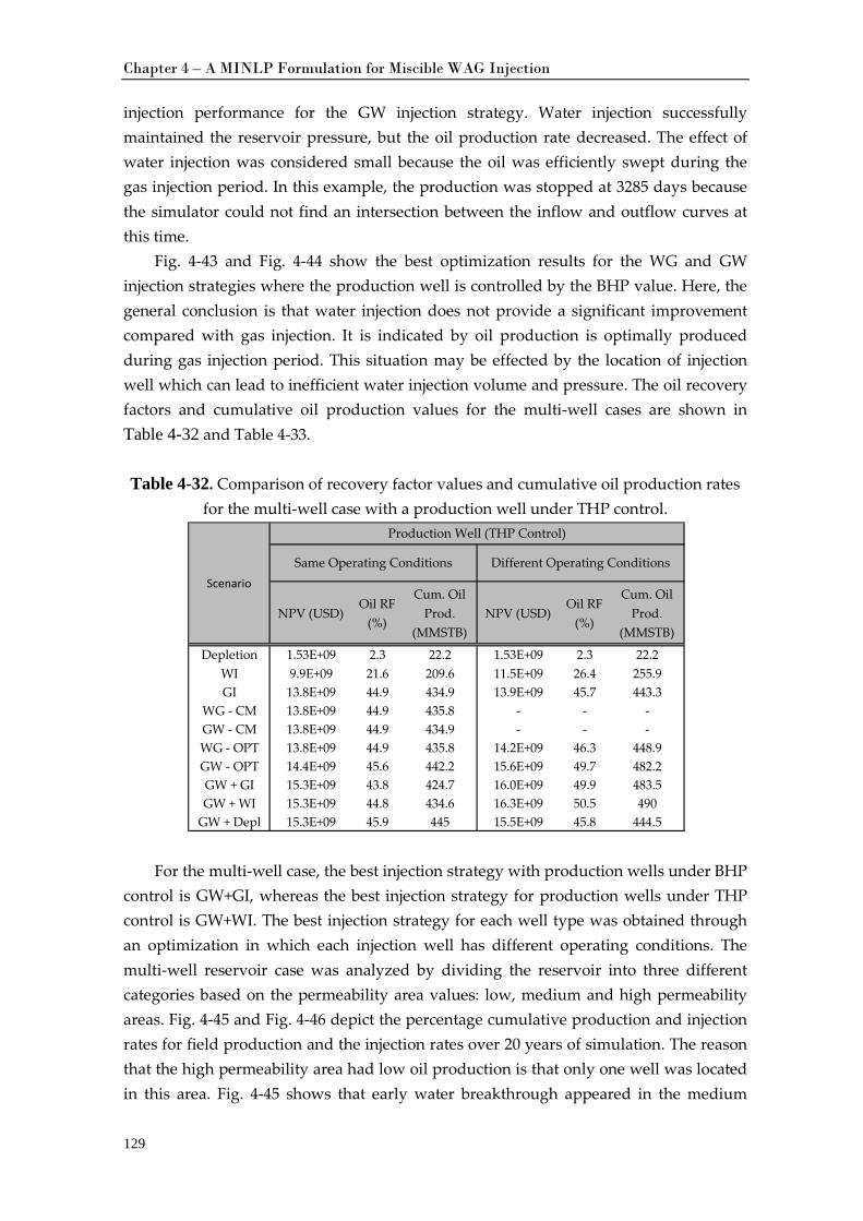
Chapter 4 – A MINLP Formulation for Miscible WAG Injection
129
injection performance for the GW injection strategy. Water injection successfully maintained the reservoir pressure, but the oil production rate decreased. The effect of water injection was considered small because the oil was efficiently swept during the gas injection period. In this example, the production was stopped at 3285 days because the simulator could not find an intersection between the inflow and outflow curves at this time.
Fig. 4-43 and Fig. 4-44 show the best optimization results for the WG and GW injection strategies where the production well is controlled by the BHP value. Here, the general conclusion is that water injection does not provide a significant improvement compared with gas injection. It is indicated by oil production is optimally produced during gas injection period. This situation may be effected by the location of injection well which can lead to inefficient water injection volume and pressure. The oil recovery factors and cumulative oil production values for the multi-well cases are shown in Table 4-32 and Table 4-33.
Table 4-32. Comparison of recovery factor values and cumulative oil production rates
for the multi-well case with a production well under THP control.
For the multi-well case, the best injection strategy with production wells under BHP control is GW+GI, whereas the best injection strategy for production wells under THP control is GW+WI. The best injection strategy for each well type was obtained through an optimization in which each injection well has different operating conditions. The multi-well reservoir case was analyzed by dividing the reservoir into three different categories based on the permeability area values: low, medium and high permeability areas. Fig. 4-45 and Fig. 4-46 depict the percentage cumulative production and injection rates for field production and the injection rates over 20 years of simulation. The reason that the high permeability area had low oil production is that only one well was located in this area. Fig. 4-45 shows that early water breakthrough appeared in the medium
NPV (USD)Oil RF
(%)
Cum. Oil Prod.
(MMSTB)NPV (USD)
Oil RF (%)
Cum. Oil Prod.
(MMSTB)
Depletion 1.53E+09 2.3 22.2 1.53E+09 2.3 22.2WI 9.9E+09 21.6 209.6 11.5E+09 26.4 255.9GI 13.8E+09 44.9 434.9 13.9E+09 45.7 443.3
WG - CM 13.8E+09 44.9 435.8 - - -GW - CM 13.8E+09 44.9 434.9 - - -WG - OPT 13.8E+09 44.9 435.8 14.2E+09 46.3 448.9GW - OPT 14.4E+09 45.6 442.2 15.6E+09 49.7 482.2GW + GI 15.3E+09 43.8 424.7 16.0E+09 49.9 483.5GW + WI 15.3E+09 44.8 434.6 16.3E+09 50.5 490
GW + Depl 15.3E+09 45.9 445 15.5E+09 45.8 444.5
Scenario
Production Well (THP Control)
Same Operating Conditions Different Operating Conditions
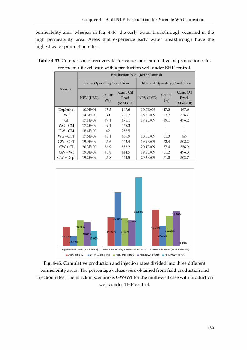
Chapter 4 – A MINLP Formulation for Miscible WAG Injection
130
permeability area, whereas in Fig. 4-46, the early water breakthrough occurred in the high permeability area. Areas that experience early water breakthrough have the highest water production rates.
Table 4-33. Comparison of recovery factor values and cumulative oil production rates
for the multi-well case with a production well under BHP control.
Fig. 4-45. Cumulative production and injection rates divided into three different
permeability areas. The percentage values were obtained from field production and injection rates. The injection scenario is GW+WI for the multi-well case with production
wells under THP control.
NPV (USD)Oil RF
(%)
Cum. Oil Prod.
(MMSTB)NPV (USD)
Oil RF (%)
Cum. Oil Prod.
(MMSTB)
Depletion 10.0E+09 17.3 167.6 10.0E+09 17.3 167.6WI 14.3E+09 30 290.7 15.6E+09 33.7 326.7GI 17.1E+09 49.1 476.1 17.2E+09 49.1 476.2
WG - CM 17.2E+09 49.1 476.3 - - -GW - CM 18.4E+09 42 258.5 - - -WG - OPT 17.6E+09 48.1 465.9 18.5E+09 51.3 497GW - OPT 19.0E+09 45.6 442.4 19.9E+09 52.4 508.2GW + GI 20.3E+09 56.9 552.2 20.4E+09 57.4 556.9GW + WI 19.0E+09 45.8 444.5 19.8E+09 51.2 496.3
GW + Depl 19.2E+09 45.8 444.5 20.3E+09 51.8 502.7
Scenario
Production Well (BHP Control)
Same Operating Conditions Different Operating Conditions
22.63%
34.01%43.36%
11.74%
64.01%
24.25%
30.58%33.40% 36.02%
28.00%
30.56%
41.40%
17.95%
81.85%
0.19%
High Permeability Area (INJ4 & PROD3) Medium Permeability Area (INJ1-3 & PROD1-2) Low Permeability Area (INJ5-8 & PROD4-5)
CUM GAS INJ CUM WATER INJ CUM OIL PROD CUM GAS PROD CUM WAT PROD
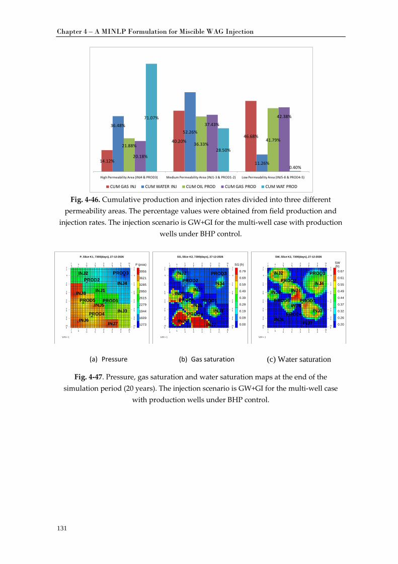
Chapter 4 – A MINLP Formulation for Miscible WAG Injection
131
PROD1
PROD2PROD3
PROD4
PROD5
INJ1
INJ2
INJ3
INJ4
INJ5
INJ6INJ7
INJ8
I1
J1
5 10
15
20
25
30
I35
J1
5 5
10
10
15
15
20
20
25
25
30
30
I1
J35
5 10
15
20
25
30
I35
J35
V/H = 1
P (psia)
3956
3621
3285
2950
2615
2279
1944
1609
1273
P, Slice K1, 7300(days), 27-12-2026
PROD1
PROD2PROD3
PROD4
PROD5
INJ1
INJ2
INJ3
INJ4
INJ5
INJ6INJ7
INJ8
I1
J1
5 10
15
20
25
30
I35
J1
5 5
10
10
15
15
20
20
25
25
30
30
I1
J35
5 10
15
20
25
30
I35
J35
V/H = 1
SG (fr)
0.79
0.69
0.59
0.49
0.39
0.29
0.19
0.09
0.00
SG, Slice K2, 7300(days), 27-12-2026
PROD1
PROD2PROD3
PROD4
PROD5
INJ1
INJ2
INJ3
INJ4
INJ5
INJ6INJ7
INJ8
I1
J1
5 10
15
20
25
30
I35
J1
5 5
10
10
15
15
20
20
25
25
30
30
I1
J35
5 10
15
20
25
30
I35
J35
V/H = 1
SW (fr)
0.67
0.61
0.55
0.49
0.44
0.37
0.32
0.26
0.20
SW, Slice K2, 7300(days), 27-12-2026
Fig. 4-46. Cumulative production and injection rates divided into three different
permeability areas. The percentage values were obtained from field production and injection rates. The injection scenario is GW+GI for the multi-well case with production
wells under BHP control.
(a) Pressure (b) Gas saturation (c) Water saturation
Fig. 4-47. Pressure, gas saturation and water saturation maps at the end of the simulation period (20 years). The injection scenario is GW+GI for the multi-well case
with production wells under BHP control.
14.12%
40.20%46.68%
36.48%52.26%
11.26%
21.88% 36.33%41.79%
20.18%
37.43%
42.38%71.07%
28.50%
0.40%
High Permeability Area (INJ4 & PROD3) Medium Permeability Area (INJ1-3 & PROD1-2) Low Permeability Area (INJ5-8 & PROD4-5)
CUM GAS INJ CUM WATER INJ CUM OIL PROD CUM GAS PROD CUM WAT PROD
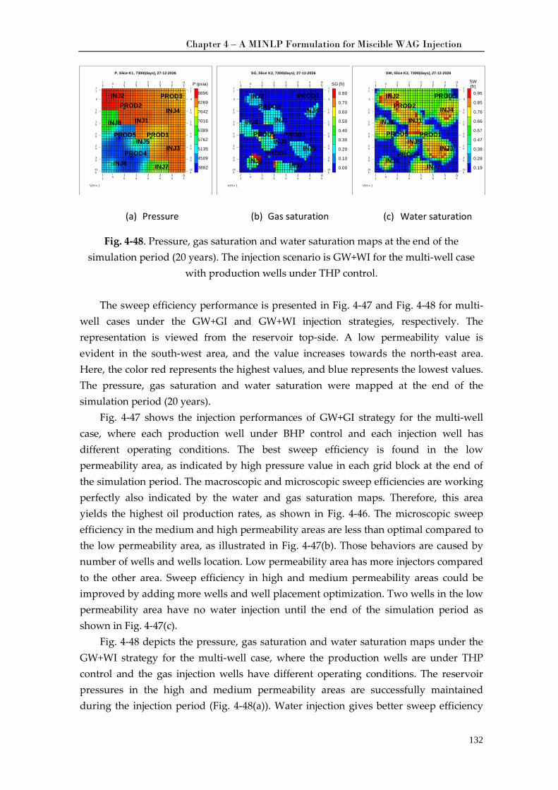
Chapter 4 – A MINLP Formulation for Miscible WAG Injection
132
PROD1
PROD3
PROD4
PROD5
INJ1
INJ2
INJ3
INJ4
INJ5
INJ6 INJ7
INJ8
I1
J1
5 10
15
20
25
30
I35
J1
5 5
10
10
15
15
20
20
25
25
30
30
I1
J35
5 10
15
20
25
30
I35
J35
V/H = 1
P (psia)
8896
8269
7642
7016
6389
5762
5135
4509
3882
P, Slice K1, 7300(days), 27-12-2026
PROD2
PROD1
PROD3
PROD4
PROD5
INJ1
INJ2
INJ3
INJ4
INJ5
INJ6INJ7
INJ8
I1
J1
5 10
15
20
25
30
I35
J1
5 5
10
10
15
15
20
20
25
25
30
30
I1
J35
5 10
15
20
25
30
I35
J35
V/H = 1
SG (fr)
0.80
0.70
0.60
0.50
0.40
0.30
0.20
0.10
0.00
SG, Slice K2, 7300(days), 27-12-2026
PROD2
PROD1
PROD3
PROD4
PROD5
INJ1
INJ2
INJ3
INJ4
INJ5
INJ6INJ7
INJ8
I1
J1
5 10
15
20
25
30
I35
J1
5 5
10
10
15
15
20
20
25
25
30
30
I1
J35
5 10
15
20
25
30
I35
J35
V/H = 1
SW (fr)
0.95
0.85
0.76
0.66
0.57
0.47
0.38
0.28
0.19
SW, Slice K2, 7300(days), 27-12-2026
PROD2
(a) Pressure (b) Gas saturation (c) Water saturation
Fig. 4-48. Pressure, gas saturation and water saturation maps at the end of the simulation period (20 years). The injection scenario is GW+WI for the multi-well case
with production wells under THP control. The sweep efficiency performance is presented in Fig. 4-47 and Fig. 4-48 for multi-
well cases under the GW+GI and GW+WI injection strategies, respectively. The representation is viewed from the reservoir top-side. A low permeability value is evident in the south-west area, and the value increases towards the north-east area. Here, the color red represents the highest values, and blue represents the lowest values. The pressure, gas saturation and water saturation were mapped at the end of the simulation period (20 years).
Fig. 4-47 shows the injection performances of GW+GI strategy for the multi-well case, where each production well under BHP control and each injection well has different operating conditions. The best sweep efficiency is found in the low permeability area, as indicated by high pressure value in each grid block at the end of the simulation period. The macroscopic and microscopic sweep efficiencies are working perfectly also indicated by the water and gas saturation maps. Therefore, this area yields the highest oil production rates, as shown in Fig. 4-46. The microscopic sweep efficiency in the medium and high permeability areas are less than optimal compared to the low permeability area, as illustrated in Fig. 4-47(b). Those behaviors are caused by number of wells and wells location. Low permeability area has more injectors compared to the other area. Sweep efficiency in high and medium permeability areas could be improved by adding more wells and well placement optimization. Two wells in the low permeability area have no water injection until the end of the simulation period as shown in Fig. 4-47(c).
Fig. 4-48 depicts the pressure, gas saturation and water saturation maps under the GW+WI strategy for the multi-well case, where the production wells are under THP control and the gas injection wells have different operating conditions. The reservoir pressures in the high and medium permeability areas are successfully maintained during the injection period (Fig. 4-48(a)). Water injection gives better sweep efficiency
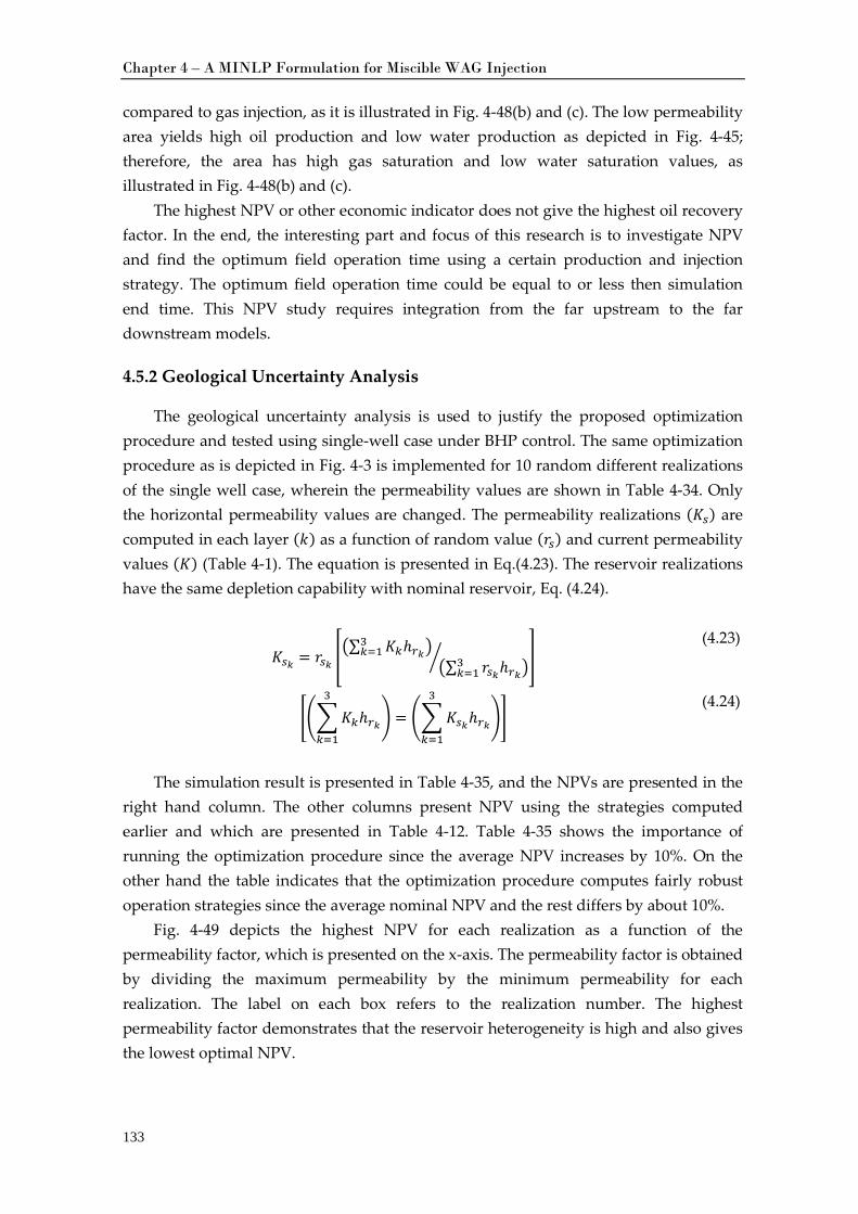
Chapter 4 – A MINLP Formulation for Miscible WAG Injection
133
compared to gas injection, as it is illustrated in Fig. 4-48(b) and (c). The low permeability area yields high oil production and low water production as depicted in Fig. 4-45; therefore, the area has high gas saturation and low water saturation values, as illustrated in Fig. 4-48(b) and (c).
The highest NPV or other economic indicator does not give the highest oil recovery factor. In the end, the interesting part and focus of this research is to investigate NPV and find the optimum field operation time using a certain production and injection strategy. The optimum field operation time could be equal to or less then simulation end time. This NPV study requires integration from the far upstream to the far downstream models.
4.5.2 Geological Uncertainty Analysis
The geological uncertainty analysis is used to justify the proposed optimization procedure and tested using single-well case under BHP control. The same optimization procedure as is depicted in Fig. 4-3 is implemented for 10 random different realizations of the single well case, wherein the permeability values are shown in Table 4-34. Only the horizontal permeability values are changed. The permeability realizations (𝐾𝑠) are computed in each layer (𝑘) as a function of random value (𝑟𝑟𝑠) and current permeability values (𝐾) (Table 4-1). The equation is presented in Eq.(4.23). The reservoir realizations have the same depletion capability with nominal reservoir, Eq. (4.24).
𝐾𝑠𝑘 = 𝑟𝑟𝑠𝑘 ��∑ 𝐾𝑘ℎ𝑟𝑘
3𝑘=1 �
�∑ 𝑟𝑟𝑠𝑘ℎ𝑟𝑘3𝑘=1 �� �
(4.23)
���𝐾𝑘ℎ𝑟𝑘
3
𝑘=1
� = ��𝐾𝑠𝑘ℎ𝑟𝑘
3
𝑘=1
�� (4.24)
The simulation result is presented in Table 4-35, and the NPVs are presented in the
right hand column. The other columns present NPV using the strategies computed earlier and which are presented in Table 4-12. Table 4-35 shows the importance of running the optimization procedure since the average NPV increases by 10%. On the other hand the table indicates that the optimization procedure computes fairly robust operation strategies since the average nominal NPV and the rest differs by about 10%.
Fig. 4-49 depicts the highest NPV for each realization as a function of the permeability factor, which is presented on the x-axis. The permeability factor is obtained by dividing the maximum permeability by the minimum permeability for each realization. The label on each box refers to the realization number. The highest permeability factor demonstrates that the reservoir heterogeneity is high and also gives the lowest optimal NPV.
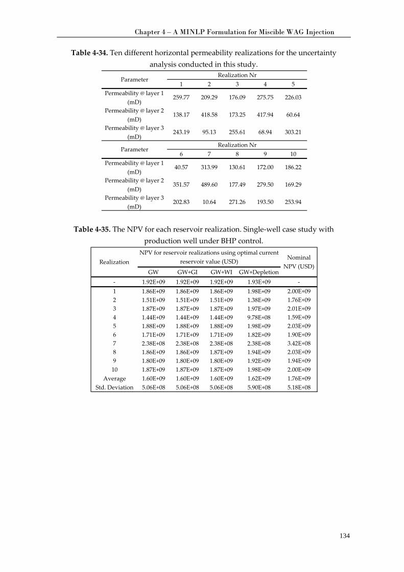
Chapter 4 – A MINLP Formulation for Miscible WAG Injection
134
Table 4-34. Ten different horizontal permeability realizations for the uncertainty analysis conducted in this study.
Table 4-35. The NPV for each reservoir realization. Single-well case study with
production well under BHP control.
1 2 3 4 5Permeability @ layer 1
(mD)259.77 209.29 176.09 275.75 226.03
Permeability @ layer 2 (mD)
138.17 418.58 173.25 417.94 60.64
Permeability @ layer 3 (mD)
243.19 95.13 255.61 68.94 303.21
6 7 8 9 10Permeability @ layer 1
(mD)40.57 313.99 130.61 172.00 186.22
Permeability @ layer 2 (mD)
351.57 489.60 177.49 279.50 169.29
Permeability @ layer 3 (mD)
202.83 10.64 271.26 193.50 253.94
Realization NrParameter
Realization NrParameter
GW GW+GI GW+WI GW+Depletion- 1.92E+09 1.92E+09 1.92E+09 1.93E+09 -1 1.86E+09 1.86E+09 1.86E+09 1.98E+09 2.00E+092 1.51E+09 1.51E+09 1.51E+09 1.38E+09 1.76E+093 1.87E+09 1.87E+09 1.87E+09 1.97E+09 2.01E+094 1.44E+09 1.44E+09 1.44E+09 9.78E+08 1.59E+095 1.88E+09 1.88E+09 1.88E+09 1.98E+09 2.03E+096 1.71E+09 1.71E+09 1.71E+09 1.82E+09 1.90E+097 2.38E+08 2.38E+08 2.38E+08 2.38E+08 3.42E+088 1.86E+09 1.86E+09 1.87E+09 1.94E+09 2.03E+099 1.80E+09 1.80E+09 1.80E+09 1.92E+09 1.94E+0910 1.87E+09 1.87E+09 1.87E+09 1.98E+09 2.00E+09
Average 1.60E+09 1.60E+09 1.60E+09 1.62E+09 1.76E+09Std. Deviation 5.06E+08 5.06E+08 5.06E+08 5.90E+08 5.18E+08
Nominal NPV (USD)
RealizationNPV for reservoir realizations using optimal current
reservoir value (USD)
Chapter 4 – A MINLP Formulation for Miscible WAG Injection
135
Fig. 4-49. Optimal NPV for each realization using solution approach depicted in Fig. 4-3.
Single-well case study with production well under BHP control.
To perform a more extensive uncertainty analysis 90 different realizations have been generated by adding to the 10 realizations discussed above. The ten best operating strategies computed earlier, corresponding to the nominal NPVs in Table 4-35, are tested on 99 different realizations, i.e. all realizations except for the nominal one.
The results are presented in Fig. 4-50 and Fig. 4-51. In Fig. 4-50 and Fig. 4-51, the lowest NPV is represented by the lowest dashed line in the boxplot figure, whereas the highest NPV is represented by the highest dashed line in the boxplot figure. The boxplot itself represents quartiles 1, 2 and 3 for each set of data. The brown circle (points) represent the average NPV while the red circle points in Fig. 4-50 represent the optimal NPV for the corresponding realization on the x-axis. Fig. 4-50 demonstrates that the optimum operating conditions for realizations 9, 7, 6, 4, and 2 involve unpromising injection strategies because they provide the lowest maximum NPVs in comparison to the other optimal operating conditions that are associated with realizations 1, 3, 5, 8, and 10. Fig. 4-51 demonstrates the best injection strategy based on geological uncertainty analysis using 10 realizations. The best injection strategy is arguable depending on the preferences of the reader, however, based on the authors’ point of view, the best injection strategy is GW+GI because this injection strategy provides the highest NPV. Other readers may insist that GW, GW+WI, or GW+depletion is the best injection strategy.
The final opinion regarding the best injection strategy is left to the reader; however, one conclusion that can be made that is the best injection strategy always begins with gas injection. Water injection and WG combinatorial strategies are not promising strategies. The results that were obtained from the uncertainty analysis depict the same conclusion, that is, the best injection strategy is GW+GI, as represented by realizations 1,
1
2
3
4
56
7
89 10
0.00E+00
5.00E+08
1.00E+09
1.50E+09
2.00E+09
2.50E+09
1.9 4.4 1.5 6.1 5.0 8.7 46.0 2.1 1.6 1.5
Opt
imum
NPV
(USD
)
Permeability Factor
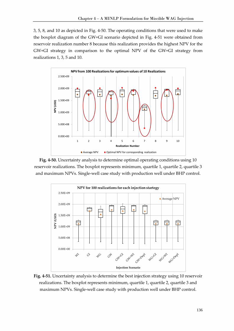
Chapter 4 – A MINLP Formulation for Miscible WAG Injection
136
3, 5, 8, and 10 as depicted in Fig. 4-50. The operating conditions that were used to make the boxplot diagram of the GW+GI scenario depicted in Fig. 4-51 were obtained from reservoir realization number 8 because this realization provides the highest NPV for the GW+GI strategy in comparison to the optimal NPV of the GW+GI strategy from realizations 1, 3, 5 and 10.
Fig. 4-50. Uncertainty analysis to determine optimal operating conditions using 10
reservoir realizations. The boxplot represents minimum, quartile 1, quartile 2, quartile 3 and maximum NPVs. Single-well case study with production well under BHP control.
Fig. 4-51. Uncertainty analysis to determine the best injection strategy using 10 reservoir
realizations. The boxplot represents minimum, quartile 1, quartile 2, quartile 3 and maximum NPVs. Single-well case study with production well under BHP control.
0.00E+00
5.00E+08
1.00E+09
1.50E+09
2.00E+09
2.50E+09
1 2 3 4 5 6 7 8 9 10
NPV
(USD
)
Realization Number
NPV from 100 Realizations for optimum values of 10 Realizations
Average NPV Optimal NPV for corresponding realization
0.00E+00
5.00E+08
1.00E+09
1.50E+09
2.00E+09
2.50E+09
NPV
(USD
)
Injection Scenario
NPV for 100 realizations for each injection startegy
Average NPV
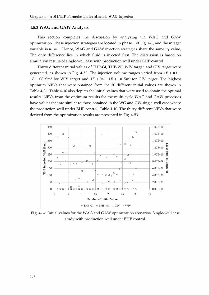
Chapter 4 – A MINLP Formulation for Miscible WAG Injection
137
4.5.3 WAG and GAW Analysis
This section completes the discussion by analyzing via WAG and GAW optimization. These injection strategies are located in phase 1 of Fig. 4-1, and the integer variable is 𝑢1 = 1. Hence, WAG and GAW injection strategies share the same 𝑢1 value, The only difference lies in which fluid is injected first. The discussion is based on simulation results of single-well case with production well under BHP control.
Thirty different initial values of THP-GI, THP-WI, WIV target, and GIV target were generated, as shown in Fig. 4-52. The injection volume ranges varied from 1𝐸 + 03 −1𝐸 + 08 Sm3 for WIV target and 1𝐸 + 04 − 1𝐸 + 10 Sm3 for GIV target. The highest optimum NPVs that were obtained from the 30 different initial values are shown in Table 4-36. Table 4-36 also depicts the initial values that were used to obtain the optimal results. NPVs from the optimum results for the multi-cycle WAG and GAW processes have values that are similar to those obtained in the WG and GW single-well case where the production well under BHP control, Table 4-10. The thirty different NPVs that were derived from the optimization results are presented in Fig. 4-53.
Fig. 4-52. Initial values for the WAG and GAW optimization scenarios. Single-well case
study with production well under BHP control.
0.00E+00
2.00E+09
4.00E+09
6.00E+09
8.00E+09
1.00E+10
1.20E+10
1.40E+10
1.60E+10
1.80E+10
0
50
100
150
200
250
300
350
400
450
0 5 10 15 20 25 30 35
Inje
ctio
n Vo
lum
e (S
m3 )
THP
Inje
ctio
n W
ell (
bara
)
Number of Initial Value
THP-GI THP-WI GIV WIV
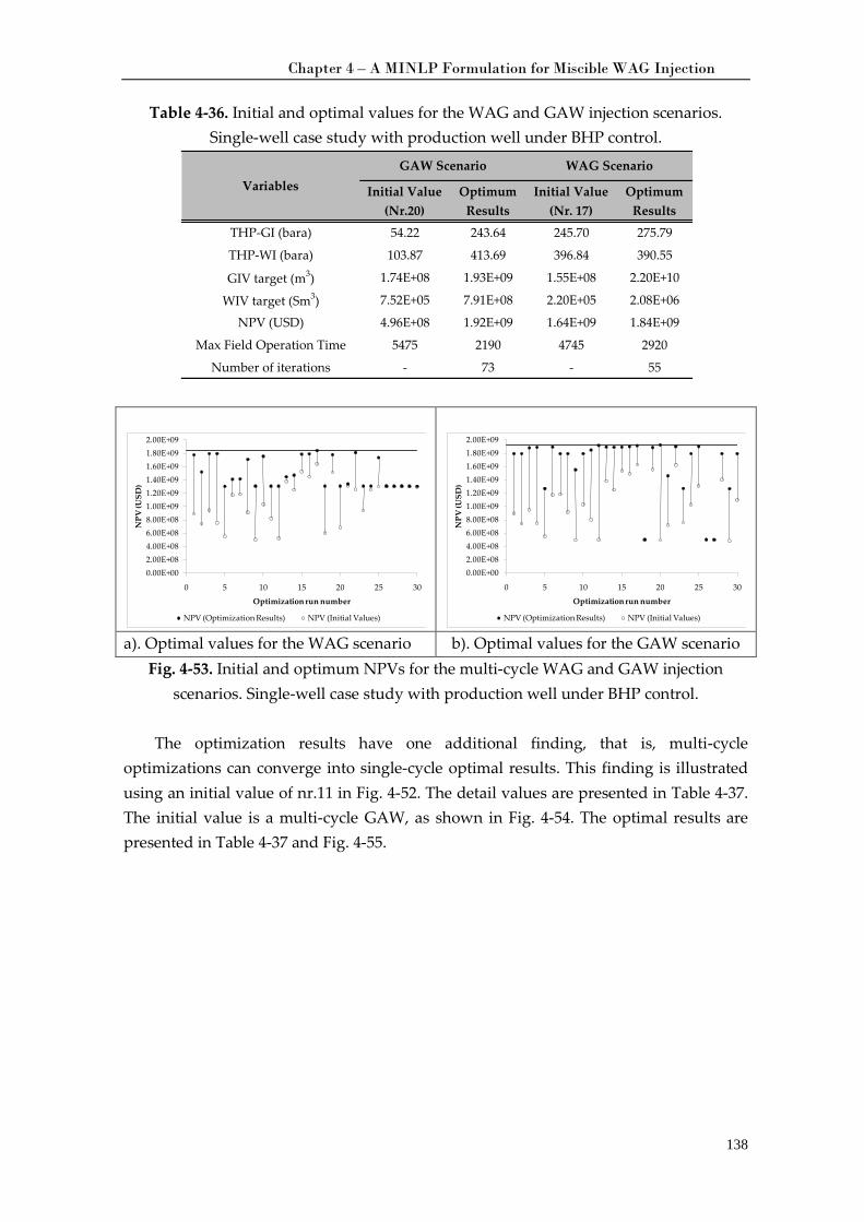
Chapter 4 – A MINLP Formulation for Miscible WAG Injection
138
Table 4-36. Initial and optimal values for the WAG and GAW injection scenarios. Single-well case study with production well under BHP control.
a). Optimal values for the WAG scenario b). Optimal values for the GAW scenario
Fig. 4-53. Initial and optimum NPVs for the multi-cycle WAG and GAW injection scenarios. Single-well case study with production well under BHP control.
The optimization results have one additional finding, that is, multi-cycle
optimizations can converge into single-cycle optimal results. This finding is illustrated using an initial value of nr.11 in Fig. 4-52. The detail values are presented in Table 4-37. The initial value is a multi-cycle GAW, as shown in Fig. 4-54. The optimal results are presented in Table 4-37 and Fig. 4-55.
Initial Value (Nr.20)
Optimum Results
Initial Value (Nr. 17)
Optimum Results
THP-GI (bara) 54.22 243.64 245.70 275.79
THP-WI (bara) 103.87 413.69 396.84 390.55
GIV target (m3) 1.74E+08 1.93E+09 1.55E+08 2.20E+10
WIV target (Sm3) 7.52E+05 7.91E+08 2.20E+05 2.08E+06
NPV (USD) 4.96E+08 1.92E+09 1.64E+09 1.84E+09
Max Field Operation Time 5475 2190 4745 2920
Number of iterations - 73 - 55
VariablesGAW Scenario WAG Scenario
0.00E+002.00E+084.00E+086.00E+088.00E+081.00E+091.20E+091.40E+091.60E+091.80E+092.00E+09
0 5 10 15 20 25 30
NPV
(USD
)
Optimization run number
NPV (Optimization Results) NPV (Initial Values)
0.00E+002.00E+084.00E+086.00E+088.00E+081.00E+091.20E+091.40E+091.60E+091.80E+092.00E+09
0 5 10 15 20 25 30
NPV
(USD
)
Optimization run number
NPV (Optimization Results) NPV (Initial Values)
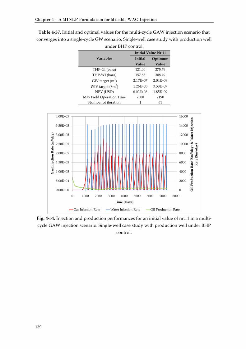
Chapter 4 – A MINLP Formulation for Miscible WAG Injection
139
Table 4-37. Initial and optimal values for the multi-cycle GAW injection scenario that converges into a single-cycle GW scenario. Single-well case study with production well
under BHP control.
Fig. 4-54. Injection and production performances for an initial value of nr.11 in a multi-cycle GAW injection scenario. Single-well case study with production well under BHP
control.
Initial Value
Optimum Value
THP-GI (bara) 121.00 275.79THP-WI (bara) 157.85 308.49GIV target (m3) 2.17E+07 2.04E+09
WIV target (Sm3) 1.26E+05 3.58E+07NPV (USD) 8.03E+08 1.85E+09
Max Field Operation Time 7300 2190Number of iteration 1 61
VariablesInitial Value Nr 11
0
2000
4000
6000
8000
10000
12000
14000
16000
0.00E+00
5.00E+04
1.00E+05
1.50E+05
2.00E+05
2.50E+05
3.00E+05
3.50E+05
4.00E+05
0 1000 2000 3000 4000 5000 6000 7000 8000O
il Pr
oduc
tion
Rat
e (S
m3 /d
ay) &
Wat
er In
ject
ion
Rat
e (S
m3 /d
ay)
Gas
Inje
ctio
n R
ate
(m3 /d
ay)
Time (Days)
Gas Injection Rate Water Injection Rate Oil Production Rate
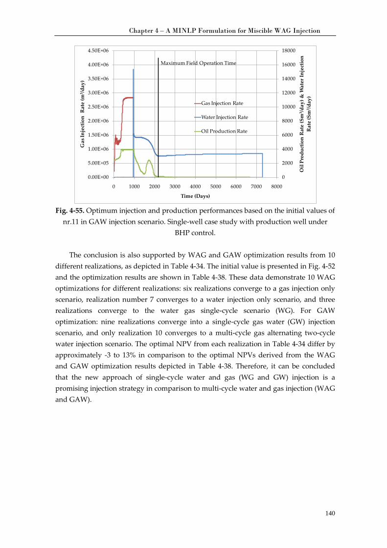
Chapter 4 – A MINLP Formulation for Miscible WAG Injection
140
Fig. 4-55. Optimum injection and production performances based on the initial values of
nr.11 in GAW injection scenario. Single-well case study with production well under BHP control.
The conclusion is also supported by WAG and GAW optimization results from 10
different realizations, as depicted in Table 4-34. The initial value is presented in Fig. 4-52 and the optimization results are shown in Table 4-38. These data demonstrate 10 WAG optimizations for different realizations: six realizations converge to a gas injection only scenario, realization number 7 converges to a water injection only scenario, and three realizations converge to the water gas single-cycle scenario (WG). For GAW optimization: nine realizations converge into a single-cycle gas water (GW) injection scenario, and only realization 10 converges to a multi-cycle gas alternating two-cycle water injection scenario. The optimal NPV from each realization in Table 4-34 differ by approximately -3 to 13% in comparison to the optimal NPVs derived from the WAG and GAW optimization results depicted in Table 4-38. Therefore, it can be concluded that the new approach of single-cycle water and gas (WG and GW) injection is a promising injection strategy in comparison to multi-cycle water and gas injection (WAG and GAW).
0
2000
4000
6000
8000
10000
12000
14000
16000
18000
0.00E+00
5.00E+05
1.00E+06
1.50E+06
2.00E+06
2.50E+06
3.00E+06
3.50E+06
4.00E+06
4.50E+06
0 1000 2000 3000 4000 5000 6000 7000 8000
Oil
Prod
uctio
n R
ate
(Sm
3 /day
) & W
ater
Inje
ctio
n R
ate
(Sm
3 /day
)
Gas
Inje
ctio
n R
ate
(m3 /d
ay)
Time (Days)
Gas Injection Rate
Water Injection Rate
Oil Production Rate
Maximum Field Operation Time
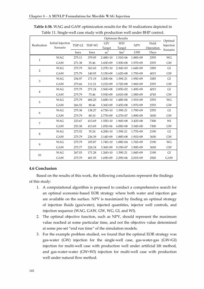
Chapter 4 – A MINLP Formulation for Miscible WAG Injection
141
Table 4-38. WAG and GAW optimization results for the 10 realizations depicted in Table 11. Single-well case study with production well under BHP control.
4.6 Conclusion
Based on the results of this work, the following conclusions represent the findings of this study:
1. A computational algorithm is proposed to conduct a comprehensive search for an optimal economic-based EOR strategy where both water and injection gas are available on the surface. NPV is maximized by finding an optimal strategy of injection fluids (gas/water), injected quantities, injector well controls, and injection sequence (WAG, GAW, GW, WG, GI, and WI).
2. The optimal objective function, such as NPV, should represent the maximum value reached at some particular time, and not the objective value determined at some pre-set “end run time” of the simulation models.
3. For the example problem studied, we found that the optimal EOR strategy was gas-water (GW) injection for the single-well case, gas-water-gas (GW+GI) injection for multi-well case with production well under artificial lift method, and gas-water-water (GW+WI) injection for multi-well case with production well under natural flow method.
THP-GI THP-WI GIV Target
WIV Target
NPV Field Operation
bara bara m3 Sm3 USD Days
WAG 275.11 379.95 2.48E+10 1.51E+06 1.88E+09 2555 WG
GAW 271.38 35.46 3.43E+09 3.50E+08 1.97E+09 2555 GW
WAG 275.79 363.43 2.27E+10 2.36E+03 1.64E+09 3285 GI
GAW 275.79 140.95 5.15E+09 1.62E+08 1.75E+09 4015 GW
WAG 254.97 171.19 3.20E+06 1.59E-21 1.95E+09 3285 GI
GAW 275.66 111.21 3.21E+09 3.72E+08 1.96E+09 2555 GW
WAG 275.79 271.24 3.56E+08 2.85E+02 1.49E+09 4015 GI
GAW 275.79 75.46 5.93E+09 4.81E+08 1.58E+09 4745 GW
WAG 275.79 406.20 3.68E+10 1.48E+06 1.91E+09 2555 WG
GAW 266.52 88.46 3.36E+09 3.45E+08 1.97E+09 2555 GW
WAG 275.38 138.27 4.73E+10 1.59E-21 1.79E+09 2555 GI
GAW 275.79 80.10 2.77E+09 6.27E+07 1.89E+09 3650 GW
WAG 223.67 413.69 1.55E+10 1.96E+08 3.42E+08 7300 WI
GAW 253.38 413.69 1.05E+06 4.08E+08 3.54E+08 7300 GW
WAG 273.52 35.24 4.20E+10 1.59E-21 1.77E+09 2190 GI
GAW 275.79 236.39 3.14E+09 1.88E+08 1.91E+09 3650 GW
WAG 275.79 105.87 1.74E+10 1.08E+04 1.76E+09 2190 WG
GAW 275.77 224.18 3.36E+09 9.19E+07 1.90E+09 3650 GW
WAG 267.03 171.28 1.26E+10 1.59E-21 1.84E+09 2190 GI
GAW 275.79 401.95 1.69E+09 2.29E+06 2.01E+09 2920 GAW
Realization
5
6
7
8
9
10
4
Initial Injection Scenario
Optimum ResultsOptimal Injection Scenario
1
2
3

Chapter 4 – A MINLP Formulation for Miscible WAG Injection
142
4. Geological uncertainty analysis to determine the best injection strategy using 10 reservoir realizations has been conducted for the single-well case study with production well under BHP control. The best injection strategy is arguable between GW, GW+GI, GW+WI, or GW+depletion due to all the scenarios have almost similar maximum NPV.
5. For single- and multi-well cases studied, the higher-cost artificial lift strategy was preferable as compared to natural flow.
6. This study shows that optimization for multi-cycle (WAG/GAW) injection strategy can converge to single-cycle (WG/GW) injection strategy.
143
Chapter 5
Summary and Suggestions for Future Work
New concepts for the improvement of oil and gas production introduced in this research show positive results. Different areas of research were covered, including unconventional gas reservoirs as well as conventional oil and gas reservoirs. The fluid flow is represented with either black-oil or compositional models. A derivative-free optimization method, the Nelder-Mead Simplex, is the only optimization algorithm that is used to solve optimization problems, (see chapters 3 and 4). The two test cases show that the Nelder-Mead Simplex method is sufficient to solve the optimization problems. The case examples presented in chapters 2, 3 and 4 use hypothetical data but represent realistic field cases. Below is a summary highlighting the major results and possibilities for improvement:
Chapter 2:
1. Reservoir model. Layered (no-cross flow) reservoir is an interesting topic to investigate in order to examine each layer performances during shut-in.
Production improvement for unconventional liquid-loading gas wells has been achieved by introducing a shut-in cycle strategy. Dry gas (black-oil) was used as the fluid model. The onset of liquid-loading was assumed when gas production was below a certain value, and the cycle shut-in was applied immediately after that. The simulation results show that the cyclic shut-in application successfully increased ultimate recovery compared with the liquid-loading case without any treatment. Simulations of cyclic shut-in have been made for a wide range of reservoirs including vertical wells with lower permeability, and horizontal multi-fractured wells. The proposed methodology has the greatest potential and is applicable to any low permeability gas reservoir, e.g., shale-gas and tight-gas reservoirs. Suggestions for future work are the following:
2. Economic model. An economic model has not yet been formulated. The economic model is of course tightly connected to the present model and can be used to obtain an economic measure for sensitivity analysis and optimization.
3. Optimization. The optimization problem can be seen as maximizing gas production or Net Present Value (NPV) with decision variables consisting of cyclic shut-in time, the number of fractures, the fracture half-length, the fracture area and well spacing. A heterogeneous reservoir area and a multi-well study will add interest to the problem.
Chapter 5 – Summary and Suggestions for Future Work
144
4. Integrated Model. As mentioned before, in this study, the occurrence of liquid-loading is assumed when the gas production rate is less than a certain value. An integrated model, including at least reservoir and well models, is needed to find actual liquid-loading occurrences. Different fluid properties, e.g., multi-phase fluid properties, may be introduced and may possibly result in different performance on the cyclic shut-in strategy application.
Chapter 3:
The major model consists of three reservoir models that meet in one surface process model and an economic model. Some researchers prefer to have a proxy or surrogate model to represent the integrated model, but high quality of fitting is necessary to obtain correct surrogate models. The integrated model needed special attention regarding the simulation time. The reservoir and surface process models have different simulation times. The reservoir is usually simulated over a longer time than the surface process. The gap is bridged by the average rate (in this study is called as project time step), and it is assumed that the rate is constant for several days and that the surface process input is the average of the reservoir output. The simulation for each reservoir time step is possible but was not necessary unless the reservoir output exhibits large variations from the previous time step caused by changing injection and production strategies, fluid composition, or surface variables (i.e., wellhead pressure or choke opening).
Chapter 3 proposed an integrated model and an optimization formulation for a complex benchmark case. The integrated model in this research was defined from downstream to upstream, including reservoir, well, pipeline, and surface process, and ended with an economic calculation. The main objective of this study was to demonstrate that an integrated simulation system can be readily developed using available commercial software technology and that integrated simulation is a feasible and interesting approach to petroleum production. The integrated simulation system in this case is easy to use, maintain and upgrade.
The automated data transfers and calculations in dynamically linked systems are a necessary condition to conduct studies that involve repeated calculations of one or several subsystems. The characteristic of an integrated system extensively models the maintenance, modification, and upgrading of the system, provided that such changes are performed in a way that communication protocols are not violated. Based on these experiences, improvements can be made as follow:
1. Uncertainty study. Introducing geological uncertainty and price forecasting have additional advantages for demonstrating the robustness of the optimization method.
2. Optimization. The core idea of this study is to maximize the sweep efficiency through gas injection for gas condensate reservoirs and water alternating gas (WAG) injection for oil reservoirs, and therefore alternative drilling optimization problems such as the number of wells and well location may be introduced. The
Chapter 5 – Summary and Suggestions for Future Work
145
current number of wells and well locations were determined based on engineering judgments. Another interesting optimization problem for this integrated model is field in-phasing with field gas production rate as constraints.
3. Fluid characterization. The fluid characterization in this integrated model can be transformed into Black-oil with BOz delumping instead of EOS to reduce CPU time.
4. Closed-loop optimization approach. The optimization presented in this study is an open-loop approach, and the results may be improved by introducing a closed-loop optimization approach (e.g. Model Predictive Control). A proxy model needs to be introduced and involved in a closed-loop approach to reduce simulation time.
Chapter 4:
1. Optimization. The current optimization problem focuses on the variables in the injector, and improvement can be made by optimizing the producer with the decision variables such as pressure or rate. The optimization method that was used could be replaced by a Branch & Bound MINLP solver. Another interesting optimization problem is optimization of the number of wells and well location.
The optimization for different injection and production scenarios in oil reservoirs were discussed, and a problem formulation was systematically developed for single-cycle injection (water-gas and gas-water), multi-cycle injection (water alternating gas and gas alternating water), continuous injection (gas injection and water injection), and combination scenarios. Two production strategies were simulated, i.e., natural flow and artificial lift. The objective function was to maximize the economic model (NPV). The problem was formulated as an MINLP problem and solved with a heuristic method. The results show that with the optimization formulation, multi-cycle injection may for instance converge to single-cycle injection. The proposed methodology is applicable to any oil reservoir where gas and water injection is available. Suggestions for future research are as follows:
2. Integrated field model and optimization. The problem could be included in an integrated model and optimization problem. Complexity would increase but, the problem would also be represented more accurately because the problem involves the re-injection of gas and water.
3. Real case implementation. Take an existing reservoir model, then setup an automated strategy (e.g. in Pipe-It) to test alternative multi-cycle WAG, single-cycle WG, and continuous (water or gas) injection scenarios for (i). a given set of fixed well locations, and (ii). with some well location flexibility
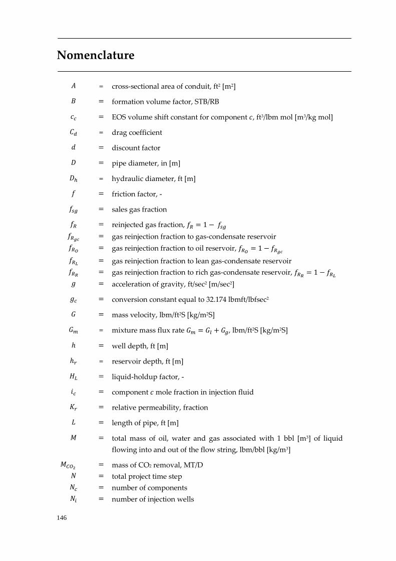
146
Nomenclature
𝐴 = cross-sectional area of conduit, ft2 [m2]
𝐵 = formation volume factor, STB/RB
𝑐𝑐 = EOS volume shift constant for component 𝑐, ft3/lbm mol [m3/kg mol]
𝐶𝑑 = drag coefficient
𝑑𝑑 = discount factor
𝐷𝐷 = pipe diameter, in [m]
𝐷𝐷ℎ = hydraulic diameter, ft [m]
𝑓 = friction factor, -
𝑓𝑠𝑔 = sales gas fraction
𝑓𝑅 = reinjected gas fraction, 𝑓𝑅 = 1 − 𝑓𝑠𝑔 𝑓𝑅𝑔𝑐 = gas reinjection fraction to gas-condensate reservoir 𝑓𝑅𝑂 = gas reinjection fraction to oil reservoir, 𝑓𝑅𝑂 = 1 − 𝑓𝑅𝑔𝑐 𝑓𝑅𝐿 = gas reinjection fraction to lean gas-condensate reservoir 𝑓𝑅𝑅 = gas reinjection fraction to rich gas-condensate reservoir, 𝑓𝑅𝑅 = 1 − 𝑓𝑅𝐿 𝑔𝑔 = acceleration of gravity, ft/sec2 [m/sec2]
𝑔𝑔𝑐 = conversion constant equal to 32.174 lbmft/lbfsec2
𝐺 = mass velocity, lbm/ft2S [kg/m2S]
𝐺𝑚 = mixture mass flux rate 𝐺𝑚 = 𝐺𝑙 + 𝐺𝑔, lbm/ft2S [kg/m2S]
ℎ = well depth, ft [m]
ℎ𝑟 = reservoir depth, ft [m]
𝐻𝐿 = liquid-holdup factor, -
𝑖𝑖𝑐 = component 𝑐 mole fraction in injection fluid
𝐾𝑟 = relative permeability, fraction
𝐿𝐿 = length of pipe, ft [m]
𝑀 = total mass of oil, water and gas associated with 1 bbl [m3] of liquid flowing into and out of the flow string, lbm/bbl [kg/m3]
𝑀𝐶𝑂2 = mass of CO2 removal, MT/D 𝑁𝑁 = total project time step 𝑁𝑁𝑐 = number of components 𝑁𝑁𝑖 = number of injection wells
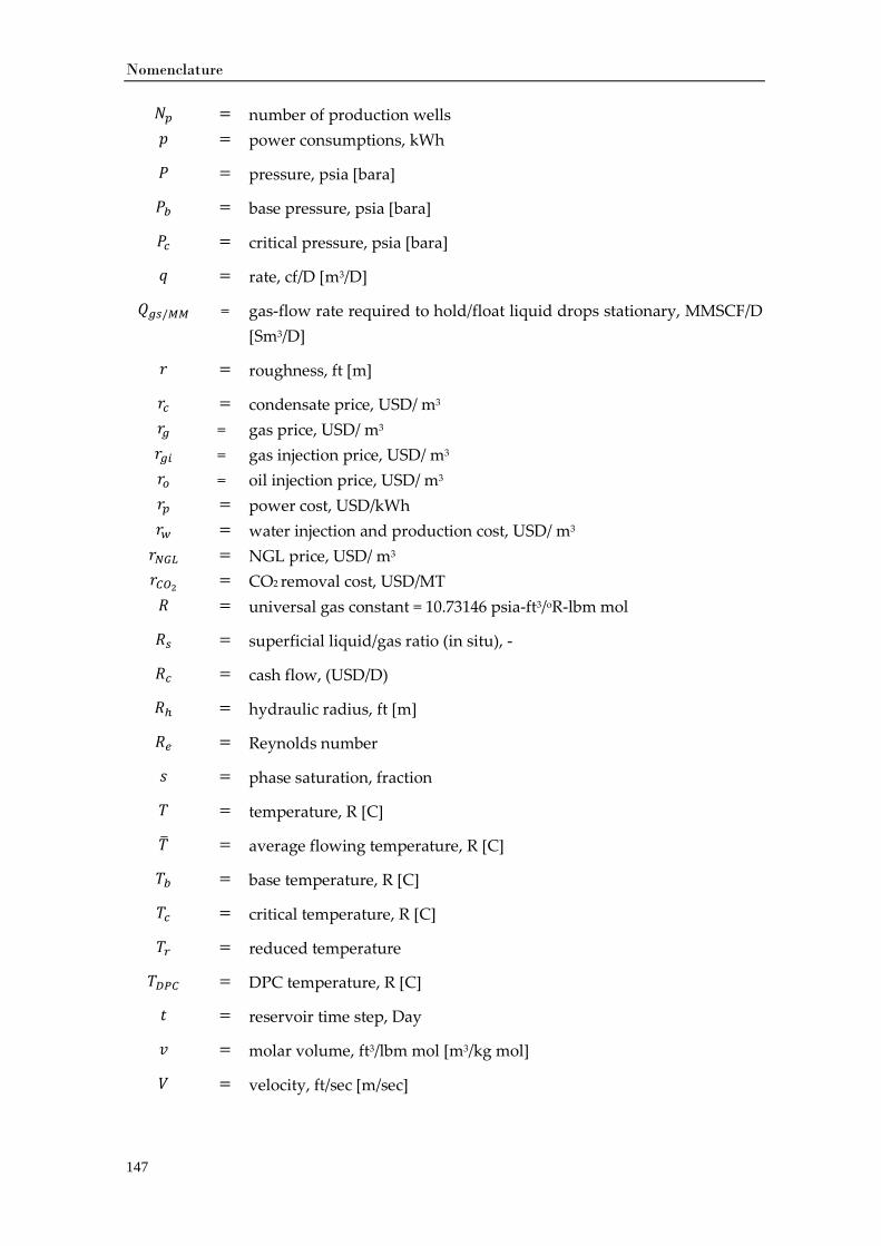
Nomenclature
147
𝑁𝑁𝑝 = number of production wells 𝑠𝑠 = power consumptions, kWh
𝑃𝑃 = pressure, psia [bara]
𝑃𝑃𝑏 = base pressure, psia [bara]
𝑃𝑃𝑐 = critical pressure, psia [bara]
𝑞𝑞 = rate, cf/D [m3/D]
𝑄𝑔𝑠/𝑀𝑀 = gas-flow rate required to hold/float liquid drops stationary, MMSCF/D [Sm3/D]
𝑟𝑟 = roughness, ft [m]
𝑟𝑟𝑐 = condensate price, USD/ m3 𝑟𝑟𝑔 = gas price, USD/ m3 𝑟𝑟𝑔𝑖 = gas injection price, USD/ m3 𝑟𝑟𝑜 = oil injection price, USD/ m3 𝑟𝑟𝑝 = power cost, USD/kWh 𝑟𝑟𝑤 = water injection and production cost, USD/ m3 𝑟𝑟𝑁𝐺𝐿 = NGL price, USD/ m3 𝑟𝑟𝐶𝑂2 = CO2 removal cost, USD/MT 𝑅 = universal gas constant = 10.73146 psia-ft3/oR-lbm mol
𝑅𝑠 = superficial liquid/gas ratio (in situ), -
𝑅𝑐 = cash flow, (USD/D)
𝑅ℎ = hydraulic radius, ft [m]
𝑅𝑒 = Reynolds number
𝑠𝑠 = phase saturation, fraction
𝑇𝑇 = temperature, R [C]
𝑇𝑇� = average flowing temperature, R [C]
𝑇𝑇𝑏 = base temperature, R [C]
𝑇𝑇𝑐 = critical temperature, R [C]
𝑇𝑇𝑟 = reduced temperature
𝑇𝑇𝐷𝑃𝐶 = DPC temperature, R [C]
𝑡 = reservoir time step, Day
𝑣 = molar volume, ft3/lbm mol [m3/kg mol]
𝑉 = velocity, ft/sec [m/sec]
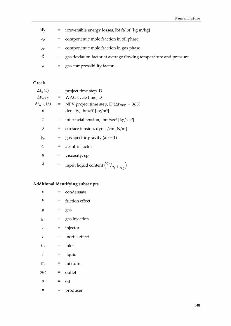
Nomenclature
148
𝑊𝑓 = irreversible energy losses, lbf ft/lbf [kg m/kg]
𝑥𝑐 = component 𝑐 mole fraction in oil phase
𝑦𝑐 = component 𝑐 mole fraction in gas phase
�̅� = gas deviation factor at average flowing temperature and pressure
𝑧 = gas compressibility factor
Greek
∆𝑡𝑝(𝑡) = project time step, D ∆𝑡𝑊𝐴𝐺 = WAG cycle time, D ∆𝑡𝑁𝑃𝑉(𝑡) = NPV project time step, D (∆𝑡𝑁𝑃𝑉 = 365)
𝜌 = density, lbm/ft3 [kg/m3]
𝜏 = interfacial tension, lbm/sec2 [kg/sec2]
𝜎 = surface tension, dynes/cm [N/m]
𝛾𝑔 = gas specific gravity (air = 1)
𝜔 = acentric factor
𝜇 = viscosity, cp
𝜆 = input liquid content �𝑞𝑞𝑙 𝑞𝑞𝑙 + 𝑞𝑞𝑔� �
Additional identifying subscripts
𝑐 = condensate
𝐹 = friction effect
𝑔𝑔 = gas
𝑔𝑔𝑖 = gas injection
𝑖𝑖 = injector
𝐼 = Inertia effect
𝑖𝑖𝑛 = inlet
𝑙𝑙 = liquid
𝑚 = mixture
𝑜𝑜𝑢𝑡 = outlet
𝑜𝑜 = oil
𝑠𝑠 = producer
Nomenclature
149
𝑟𝑟 = reservoir
𝑠𝑠 = superficial value
𝑠𝑠𝑠𝑠𝑠𝑠 = separator
𝑠𝑠𝑙𝑙 = Terminal settling
𝑤𝑤 = water
𝑤𝑤𝑖 = water injection
𝑤𝑤𝑝 = water production
𝑤𝑤𝑓 = bottomhole production well
𝑤𝑤ℎ = well-head production well
150
References
AbdulKarim, A., Al-Dhubaib, T., Elrafie, E., & ALamoudi, M. (2010). Overview of Saudi Aramco’s Intelligent Field Program. Paper SPE 129706. Presented at SPE Intelligent Energy Conference and Exhibition, 23-25 March 2010, Utrecht, The Netherlands. Society of Petroleum Engineers. doi:10.2118/129706-MS
Amro, A. A. B., Sakaria, D., Lestariono, Y., McAlonan, N., & Shere, A. J. (2010). Benefits From Implementing an Integrated Asset Operations Modelling System. Paper SPE 127893. Presented at SPE Intelligent Energy Conference and Exhibition, 23-25 March 2010, Utrecht, The Netherlands.
Aspen HYSYS User Guide. (2004). Aspen Technology, Inc.
Awan, A., Teigland, R., & Kleppe, J. (2008). A Survey of North Sea Enhanced-Oil-Recovery Projects Initiated During the Years 1975 to 2005. Paper SPE 99546. SPE Reservoir Evaluation & Engineering, 11(3), 497-512. doi:10.2118/99546-PA
Bailey, W. J., Couët, Benoît, & Wilkinson, David. (2005). Framework for Field Optimization To Maximize Asset Value. Paper SPE 87026. SPE Reservoir Evaluation & Engineering, (Issue December 2004).
Barroux, C. C., Duchet-Suchaux, P., Samier, P., & Nabil, R. (2000). Linking Reservoir and Surface Simulators : How to Improve the Coupled Solutions. Paper SPE 65159. Presented at SPE European Petroleum Conference, 24-25 October 2000, Paris, France. Society of Petroleum Engineers. doi:10.2523/65159-MS
Beggs, D. H., & Brill, J. P. (1973). A Study of Two-Phase Flow in Inclined Pipes. Journal of Petroleum Technology, 25(5). doi:10.2118/4007-PA
Camponogara, E., & Plucenio, A. (2008). Column Generation for Solving a Compressor Scheduling Problem. 2008 IEEE International Conference on Automation Science and Engineering (pp. 796-801). IEEE. doi:10.1109/COASE.2008.4626473
Caudle, B. H., & Dyes, A. B. (1958). Improving Miscible Displacement by Gas-Water Injection. Trans., AIME, 213, 281-284.
Christensen, J. R., Stenby, E. H., & Skauge, A. (2001). Review of WAG Field Experience. Paper SPE 71203. SPE Reservoir Evaluation & Engineering, (April).
References
151
Coleman, S. B. et al. (1991). A New Look at Predicting Gas-Well Loading-Up. Journal of Petroleum Technology, 43(3).
Couët, B., Djikpesse, H., Tonkin, T., & Wilkinson, D. (2010). Production Enhancement Through Integrated Asset Modeling Optimization. Paper SPE 135901. Presented at SPE Production And Operations Conference, 8-10 June 2010, Tunis, Tunisia.
Crogh, N., Karen, E., & Morterud, S. (2002). WAG Injection at the Statfjord Field, A Success Story. Paper SPE 78348. Presented at European Petroleum Conference, 29-31 October 2002, Aberdeen, Scotland, U.K. Society of Petroleum Engineers. doi:10.2523/78348-MS
Cullick, A. S., David, H., Keshav, N., Jay, A., & James, K. (2003). Optimizing Multiple-Field Scheduling and Production Strategy with Reduced Risk. Paper SPE 84239. Presented at SPE Annual Technical Conference and Exhibition, 5-8 October 2003, Denver, Colorado, U.S.A. Society of Petroleum Engineers. doi:10.2523/84239-MS
Daoyong, Y., Qi, Z., Huanwen, C., Hu, F., & Luhua, L. (2000). Optimization of Multivariate Production-Injection System for Water-Alternating-Gas Miscible Flooding in Pubei Oil Field. Paper SPE 62856. Presented at SPE/AAPG Western Regional Meeting, 19-23 June 2000, Long-Beach, California, U.S.A. Society of Petroleum Engineers. doi:10.2523/62856-MS
Dobbs, W., Browning, B., Killough, J., & Kumar, A. (2011). Coupled Surface / Subsurface Simulation of an Offshore K2 Field. Paper SPE 145070. Presented at SPE Annual Technical Conference and Exhibition, 30 October - 2 November 2011, Denver, Colorado, U.S.A.
Fetkovich, M. J. (1975). Multipoint Testing of Gas Wells. SPE Mid-Continental Section, Continuing Education Course, Well Testing Analysis, March 17, 1975.
Foss, B. A., & Halvorsen, I. J. (2009). Dynamic Optimization of the LNG Value Chain. Proceedings of the 1st Annual Gas Processing Symposium.
Galic, H., Cawley, S., Bishop, S., Todman, S., & Gas, F. (2009). CO2 Injection Into Depleted Gas Reservoirs. Paper SPE 123788. Presented at SPE Offshore Europe Oil & Gas Conference, 8-11 September 2009, Aberdeen, UK.
Gharbi, R. (2004). Use of Reservoir Simulation for Optimizing Recovery Performance. Journal of Petroleum Science and Engineering, 42(2-4), 183-194. doi:10.1016/j.petrol.2003.12.010
Guo, B., Ghalambor, A., & Xu, C. (2006). A Systematic Approach to Predicting Liquid Loading in Gas Wells. Paper SPE 94081. SPE Production & Operations, 21(1), 81-88. doi:10.2118/94081-PA
References
152
Hagedorn, A. R., & Brown, K. E. (1965). Experimental Study of Pressure Gradients Occuring During Continuous Two-Phase Flow in Small-Diameter Vertical Conduits. Journal of Petroleum Technology, 17(4), 475-484.
Hepguler, G., Barua, S., & Bard, W. (1997). Integration of A Field Surface and Production Network With A Reservoir Simulator. Paper SPE 38937. SPE Computer Applications, (June). doi:10.2118/38937-PA
Hepguler, G., Dutta-Roy, Kunal, & Bard, W. A. (1997). Application of A Field Surface and Production Network Simulator Integrated With A Reservooir Simulator. Paper SPE 38007. Presented at SPE Reservoir Simulation Symposium, 8-11 June 1997, Dallas, Texas, U.S.A. Society of Petroleum Engineers. doi:10.2523/38007-MS
Ikoku, C. U. (1984). Natural Gas Reservoir Engineering. New York: Wiley.
Issaka, M., Dahan, M., Alburaikan, M., & Verjan, E. (2008). Real-Time Integrated Field Management at the Desktop. Paper SPE 112071. Presented at SPE Intelligent Energy Conference and Exhibition, 25-27 February 2010, Amsterdam, The Netherlands. Society of Petroleum Engineers. doi:10.2118/112071-MS
Jansen, J.D, Bosgra, O. H., & Van den hof, P. M. J. (2008). Model-Based Control of Multiphase Flow in Subsurface Oil Reservoirs. Journal of Process Control, 18(9), 846-855. doi:10.1016/j.jprocont.2008.06.011
Jensen, T. B., Harpole, K. J., & Østhus, A. (2000). EOR Screening for Ekofisk. Paper SPE 65124. Presented at European Petroleum Conference, 24-25 October 2000, Paris, France.
Juell, A., Whitson, C. H., & Hoda, M. F. (2010). Model-Based Integration and Optimization--Gas-Cycling Benchmark. SPE Journal, 15(2). doi:10.2118/121252-PA
Kenyon, D. E., & Behie, G. A. (1987). Third SPE Comparative Solution Project: Gas Cycling of Retrograde Condensate Reservoirs. Paper SPE 12278. Journal of Petroleum Technology, 39(8), 981-997. doi:10.2118/12278-PA
Killough, J. E., & Kossack, C. A. (1987). Fifth SPE Comparative Solution Project: Evaluation of Miscible Flood Simulators. Paper SPE 16000. Presented at The Ninth SPE Symposium on Reservoir Simulation, 1-4 February 1987, San Antonio, Texas, U.S.A.
Kosmala, A., Sigurd, A., Gajraj, A., Biran, V., Brusdal, K., Stokkenes, A., & Torrens, R. (2003). Coupling of A Surface Network With Reservoir Simulation. Paper SPE 84220. Presented at SPE Annual Technical Conference and Exhibition, 5-8 October 2003, Denver, Colorado, U.S.A. Society of Petroleum Engineers. doi:10.2523/84220-MS
References
153
Kosmidis, V. D., Perkins, J. D., & Pistikopoulos, E. N. (2005). A Mixed Integer Optimization Formulation for The Well Scheduling Problem on Petroleum Fields. Computers & Chemical Engineering, 29(7), 1523-1541. doi:10.1016/j.compchemeng.2004.12.003
Kulkarni, M. M., & Rao, D. N. (2004). Experimental Investigation of Various Methods of Tertiary Gas Injection. Paper SPE 90589. Presented at SPE Annual Technical Conference and Exhibition, 26-29 September 2004, Houston, Texas, U.S.A. Society of Petroleum Engineers. doi:10.2523/90589-MS
Lagarias, J. C., Reeds, J. A., Wright, M. H., & Wright, P. E. (1998). Convergence Properties of the Nelder-Mead Simplex Method in Low Dimensions. SIAM Journal on Optimization, 9(1), 112. doi:10.1137/S1052623496303470
Lea, J. F., & Nickens, H. V. (2004). Solving Gas-Well Liquid-Loading Problems. Journal of Petroleum Technology (JPT), (April).
Lea, J. F., Nickens, H. V., & Wells, M. R. (2008). Gas Well Deliquification 2nd Edition. Elsevier Inc.
Lien, S. C., Lie, S. E., Fjellbirkeland, H., & Larsen, S. V. (1998). Brage Field, Lessons Learned After 5 Years of Production. Paper SPE 50641. Presented at SPE European Petroleum Conference, 20-22 October 1998, The Hague, The Netherlands. Society of Petroleum Engineers. doi:10.2523/50641-MS
Litvak, M., Onwunalu, J., & Baxter, J. (2011). Field Development Optimization with Subsurface Uncertainties. Paper SPE 146512. Presented at SPE Annual Technical Conference and Exhibition, 30 October - 2 November 2011, Denver, Colorado, U.S.A.
Lobato-Barradas, G., Dutta-Roy, K., Agustin, M.-R., Ozgen, C., & Firincioglu, T. (2002). Integrated Compositional Surface-Subsurface Modeling for Rate Allocation Calculations. Paper SPE 74382. Presented at SPE International Petroleum Conference and Exhibition, 10-12 February 2002, Villahermosa, Mexico. Society of Petroleum Engineers. doi:10.2523/74382-MS
Madray, R., Coll, C., Veitch, G., Chiboub, C., Butter, M., Azouzi, S., Bahri, S., et al. (2008). Integrated Field Modelling of the Miskar Field. Paper SPE 113873. Presented at SPE EUROPEC/EAGE Conference, 9-12 June 2008, Rome, Italy.
Miskimins, J. (2008). Design and Life Cycle Considerations for Unconventional Reservoir Wells. Paper SPE 114170. Presented at the SPE Unconventional Reservoirs Conference, 10-12 February, Keystone, Colorado, U.S.A. Society of Petroleum Engineers. doi:10.2118/114170-MS
References
154
Nazarian, B. (2002). Integrated field modeling. PhD Thesis, The Norwegian University of Science and Technology (NTNU), Norway.
Nelder, J. A., & Mead, R. (1965). A simplex method for function minimization. The Computer Journal, 8, 308-331.
Nocedal, J., & Wright, S. J. (2006). Numerical Optimization 2nd Edition. Springer.
Nosseir, M., Darwich, T., Sayyouh, M., & Sallaly, M. (2000). A New Approach for Accurate Prediction of Loading in Gas Wells Under Different Flowing Conditions. Paper SPE 66540. SPE Production & Facilities, 15(4), 241-246. doi:10.2118/66540-PA
Nævdal, G., Brouwer, D. R., & Jansen, J.-D. (2006). Waterflooding using closed-loop control. Computational Geosciences, 10(1), 37-60. doi:10.1007/s10596-005-9010-6
Ogunyomi, B. A., Jablonowski, C. J., & Lake, L. W. (2011). Field Development Optimization Under Uncertainty : Screening-Models for Decision Making Reservoir model. Paper SPE 146788. Presented at SPE Annual Technical Conference and Exhibition, 30 October - 2 November 2011, Denver, Colorado, U.S.A.
Panda, M., Ambrose, J., Beuhler, G., & McGguire, P. (2009). Optimized EOR Design for the Eileen West End Area, Greater Prudhoe Bay. Paper SPE 123030. SPE Reservoir Evaluation & Engineering, 12(1), 25-32. doi:10.2118/123030-PA
Petroleum Experts (IPM Tutorials). (2004). Petroleum Experts.
Pipe-It Online Documentation. (2006). Petrostreamz AS.
Rashid, K., Demirel, S., & Couët, B. (2011). Gas-Lift Optimization with Choke Control using a Mixed-Integer Nonlinear Formulation. Industrial & Engineering Chemistry Research, 50, 2971-2980. doi:dx.doi.org/10.1021/ie101205x
Rahmawati, S.D., Whitson, C.H., Foss, B., & Kuntadi, A. (2010). Multi-Field Asset Integrated Optimization Benchmark. Paper SPE 130768. Presented at SPE EUROPEC/EAGE Annual Conference and Exhibition, 14-17 June 2010, Barcelona, Spain.
Rahmawati, S.D., Whitson, C.H., & Foss, B. (2011). A Mixed-Integer Non Linear Problem Formulation for Miscible WAG Injection. Submitted to Journal of Petroleum Science & Engineering.
Rahmawati, S.D., Whitson, C.H., Foss, B., & Kuntadi, A. (2012). Integrated Field Operation and Optimization. Accepted to Journal of Petroleum Science & Engineering. doi: 10.1016/j-petrol.2011.12.027
References
155
Saputelli, L., Ramirez, K., Chegin, J., & Cullick, S. (2009). Waterflood Recovery Optimization Using Intelligent Wells and Decision Analysis. Paper SPE 120509. Presented at SPE Latin American and Caribbean Conference, 31 May - 3 June 2009, Cartagena, Colombia.
Sensor Reference Manual. (2009). Coats Engineering, Inc.
Talukdar, S., & Instefjord, R. (2008). Reservoir Management of the Gullfaks Main Field. Paper SPE 113260. Presented at SPE EUROPEC/EAGE Conference, 9-12 June 2008, Rome, Italy.
Tomasgard, A., Rømo, F., Fodstad, M., & Midthun, K. (2007). Optimization Models for the Natural Gas Value Chain. In Geometric Modeling, Numerical Simulation, and Optimization (pp. 521-558). Springer Verlag.
Trick, M. D. (1998). A Different Approach to Coupling A Reservoir Simulator With A Surface Facilities Model. Paper SPE 40001. Presented at SPE Gas Technology Symposium, 15-18 March 1998, Calgary, Alberta, Canada. Society of Petroleum Engineers. doi:10.2523/40001-MS
Turner, R. G., Hubbard, M. G., & Dukler, A. E. (1969). Analysis and Prediction of Minimum Flow Rate for the Continuous Removal of Liquid Loadings from Gas Wells. Journal of Petroleum Technology, 21(11). doi:10.2118/2198-PA
Users Manual for API 14B, SSCSV Sizing Computer Program, Second edition, Appendix B. (1978). (p. 38).
Van Essen, G. m, Zandvliet, M. J., Van Den Hof, P. m j, Bosgra, O. H., & Jansen, J.D. (2006, October). Robust Optimization of Oil Reservoir Flooding. Proceeding of 2006 IEEE International Conference on Control Applications. doi:10.1109/CCA.2006.285954
Watson, M. J., Hawkes, N. J., Pickering, P. F., Elliott, J., & Studd, L. W. (2006). Integrated Flow Assurance Modeling of Angola Block 18 Western Area Development. Paper SPE 101826. Presented at SPE Annual Technical Conference and Exhibition, 24-27 September 2006, San Antonio, Texas, U.S.A.
Whitson, C. H., & Brule, M. R. (2000). SPE Phase Behavior Monograph. Physical Review E (Vol. 20). Richardson, Texas: Society of Petroleum Engineers, Inc.
Whitson, C.H., Rahmawati, S.D., & Juell, A. (2012). Cyclic Shut-in Strategy for Liquid-loading Gas Wells. Paper SPE 153073. To be presented at the SPE/EAGE European Unconventional Resources Conference and Exhibition, 20-22 March 2012, Vienna, Austria.
156
Appendix A
HYSYS Automation
This appendix will elaborate on the HYSYS automation technique that was written in the Ruby language. Other programming languages such as: Visual Basic, VBScript, C++, or JAVA are able to interact with HYSYS since an access to automation application is language-independent. The explanation is started from opening HYSYS to saving a current HYSYS case at the end of the simulation.
Automation is defined as the ability to drive one application from another. For example, the developers of Product A have decided in their design phase that it would make their product more usable if they exposed Product A’s objects, thereby making it accessible to Automation. Since Products B, C and D all have the ability to connect to applications that have exposed objects; each can programmatically interact with Product A. In Automation terminology, the functions of an object are called methods and the variables are called properties.
Example A.1require 'win32ole'
Open HYSYS file
hymodel_path = "Process/Process-Model" hyApp = WIN32OLE.new("HYSYS.Application") curPath = Dir.getwd case_file = curPath + "/#{hymodel_path}/" + hy_file hyCase = hyApp.SimulationCases.open(case_file) hyFlowsheet = hyCase.Flowsheet
Example A.1 has been discussed previously in section 3.3.2. HYSYS is accessed through Object Link Embedding (OLE) provided by Windows; therefore win32ole needs to be called in the beginning on accessing the HYSYS file. The location of the HYSYS file must be defined with the name hymodel-path. The hyApp command is used to open HYSYS application. hyCase command opens the previously specified case that is defined in case_file. The hyFlowsheet initiates work on the flowsheet inside the hyCase.
The dot operator represents the path that is followed to get to a specific property. The path and structure of objects are referred to as the object hierarchy. The object hierarchy is an important and fundamental concept for utilizing automation. A particular property can only be accessed by following specific object hierarchy. In HYSYS the path is always begun with the SimulationCase and Application objects.
Appendix A – HYSYS Automation
157
Example A.2hyFlowsheet.MaterialStreams.Item("LeanGC").ComponentMolarFlow.Values = InputCompMolarFlow[CO2]
Enter HYSYS input values
hyFlowsheet.MaterialStreams.Item("Gas").Temperature.Value=TempGas hyFlowsheet.Operations("TeeOp").Item("TEE1").SplitsValue = SF_TEE1
In order to begin communication between user and HYSYS simulator, an initial link to the server application must be established. In HYSYS, this is accomplished through the starting objects: SimulationCase or Application. Those objects have been saved in the hyFlowsheet command, as shown in Example A.1. The link that is discussed here is the input values link.
Example A.2 provides three different HYSYS inputs. The first and second codes are linked to MaterialStreams and the last code is connected with Operations unit. The item property is specified after the MaterialStreams and Operations commands and taking a name or index value or integer number as the argument and returns a reference to the object. The last specified term is called attribute. In MaterialStreamz, we can access pressure or temperature or molar volume or etc., while in Operations, we can specify fraction value or split value or etc. The other attributes can be seen in the type library.
Example A.3hyCase.Solver.CanSolve = true
Run HYSYS simulation
hyBasis =hyCase.BasisManager hyFluidPackage = hyBasis.FluidPackages.Item(0)
The Solver is accessed from the SimulationCase object. The Solver object can be used to
turn the calculation on and off. When accessing HYSYS through Automation it is important to note that HYSYS does not allow communication while it is solving. If information is sent to HYSYS from a client application, HYSYS will not return control to the calling program until calculations are complete. If it is necessary to pass an amount of information to HYSYS it is best to turn the Solver off first and then turn it on once the information is sent.
The Basis objects refer predominantly to objects handled by the HYSYS BasisManager. The BasisManager object in HYSYS is responsible for handling the global aspects of a HYSYS simulation case. These objects include reactions, components, and property packages. The Basis Manager object is accessed through the SimulationCase object. From the BasisManager object, the FluidPackages and HypoGroups objects can be accessed. Changing the objects accesed directly or indirectly through the BasisManager such as FluidPackages, PropertyPackage, Components, and Hypotheticals requires notification to the HYSYS simulation environment.
The FluidPackages object returned by the BasisManager object is a collection object containing all FluidPackage objects in a case. Each FluidPackage object can have its own PropertyPackage object and Components object. When the Fluid Package is accessed in this way, changes can be made to the Property Package and the list of components.
Appendix A – HYSYS Automation
158
When obtaining a reference to the FluidPackage object from the Flowsheet object, the one Fluid Package associated with the Flowsheet is being accessed. The property package or component list of the Fluid Package object may be viewed, however no changes may be made.
Example A.4hyProduct_stream_MassRate = hyFlowsheet.MaterialStreams.Item("Lean GC").MassFlowValue
Get HYSYS simulation results
hyProduct_stream_MolarRate = hyFlowsheet.MaterialStreams.Item("Lean GC").MolarFlowValue
The HYSYS simulation result is taken in the same way as simulation input. The
difference lies on the command position. The command has to be on the right-side of equal sign to get simulation result value.
Example A.5hyCase.Save
HYSYS simulation save
Example A.5 is used to save the current results of HYSYS simulation.