Integrated Instrumentation Plan for

Assessing the Seismic Response of Structures­

A Review of the Current USGS Program

Integrated Instrumentation Plan for

Assessing the Seismic Response of Structures­

A Review of the Current USGS Program

By Mehmet Celebi, Erdal Safak, A. Gerald Brady, Richard Maley, and Vahid Sotoudeh

U.S. GEOLOGICAL SURVEY CIRCULAR 947

7987

Department of the Interior

DONALD PAUL HODEL, Secretary

U.S. Geological Survey

Dallas L. Peck, Director

Library of Congress Cataloging-in-Publication Data

Main entry under title: Integrated instrumentation plan for assessing the seismic response of

structures.

(U.S. Geological Survey Circular 947) Bibliography Supt. of Docs. no.: I 19.4/2:947 1. Structural dynamics. 2. Earthquake engineering Instruments. I. Celebi,

Mehmet. II. Geological Survey (U.S.) III. Series.

TA654.6.I56 1985 624.1'762 85-600306

Free on application to the Books and Open-File Reports Section, U.S. Geological Survey, Federal Center, Box 25425, Denver, CO 80225

Page Introduction----------------------- 1 Objectives-------------------------- 1 Current programs for instrumenta-

tion of structures---------------- 2 San Francisco Bay Area instru­

mentation program----------------- 2 Steps in instrumenting a structure- 4

Site visit---------------------- 5 Ambient-vibration tests--------- 6 Forced-vibration test----------- 6 Dynamic analysis---------------- 6 Installation of instruments----- 6 Maintenance--------------------- 6 Instrumentation for structural

response studies-------------- 7 Data processing----------------- 7

Examples of structural instru­mentation schemes----------------- 8

Pacific Park Plaza, Emeryville- 8 Transamerica Building, San

Francisco--------------------- 8 Great Western Savings Building,

Berkeley--------------------- 10 Computer analysis---------- 10 Ambient-vibration test----- 10 Instrumentation------------ 14

Case studies of data from instru­mented structures---------------- 14

Imperial County Services Building--------------------- 14

Meloland Road-Interstate Highway 8 overcrossing------- 15

Future instrumentation needs------- 16 Conclusions------------------------ 19 References cited------------------- 19

CONTENTS

Page Appendix A--Measurement of

structural motion---------------- 20 Introduction------------------- 20 Motion of a rigid body--------- 20

Large rotations------------ 20 Small rotations------------ 22

Plane motion------------------- 23 Large rotation------------- 23 Small rotation------------- 24

Flexible structures------------ 24 Application to vibration of

buildings-------------------- 25 Rigid floors--------------- 25 Flexible floors------------ 26

Appendix B--Analysis of ambient­vibration data------------------- 27

Natural frequencies and damping---------------------- 27

Modal amplitudes--------------- 27 Phases------------------------- 27 Example------------------------ 27 Reference---------------------- 29

Appendix C--Forced-vibration testing-------------------------- 29

References cited--------------- 30 Appendix D--Draft scheme for

instrumenting the Bay Bridge----- 31 Introduction------------------- 31 Proposed scheme---------------- 31

East suspension span------- 31 Main truss span------------ 34 Total instrumentation------ 34

Appendix E--Instrumentation related to soil-structure interaction---------------------- 35

References cited--------------- 36

ILLUSTRATIONS

Figure 1. 2.

3.

4. 5.

Page

Organizational flow chart of USGS instrumentation program-------------- 5 Typical plan view and cross section used to determine instrumentation

scheme, Pacific Park Plaza, Emeryville, California----------------- 8 Mode shapes and frequencies from vibration testing, Pacific Park

Plaza, Emeryville, California-------------------------------------- 9 Instrumentation scheme, Pacific Park Plaza, Emeryville, California----- 10 Typical elevation sections and floor plans showing locations and

types of instrumentation, Transamerica Building, San Francisco, California--------------------------------------------------------- 11

m

Figure 6.

7. a.

9.

10.

11.

12.

13.

Al-A6.

A7-A8.

Bl-B2.

B3. Dl-02.

El.

E2.

Page

Mode shapes and frequencies from vibration, testing, Transamerica Building, San Francisco, California-------------------------------- 12

Floor plan of Great Western Savings Building, Berkeley, California----- 12 Transducer locations for ambient-vibration testing, Great Western

Savings Building, Berkeley, California----------------------------- 13 Photograph of Imperial County Services Building, El Centro,

California, showing structural damage suffered during the 1979 Imperial Valley earthquake----------------------------------------- 14

Plan view showing deployment of FBA accelerometers and SMA-1 accelerograph at Imperial County Services Building, El Centro, California, and adjacent free-field site--------------------------- 15

Part of CRA-1 strong-motion accelerogram recorded on October 15, 1979, in Imperial County Services Building, El Centro, California-------- 16

Plan view showing deployment of FBA accelerometers at Meloland Road-Interstate Highway 8 overcrossing----------------------------- 17

Part of October 15, 1979, strong-motion accelerogram recorded at Meloland Road-Interstate Highway 8 overcrossing-------------------- 18

Sketches showing: Al. Motion of a rigid body in space----------------------------------- 20 A2. Rotational components of motion----------------------------------- 21 A3. Measurements for motion in space---------------------------------- 22 A4. Measurements for motion in plane---------------------------------- 23 AS. Measurements for flexible structures------------------------------ 25 A6. Measurements for structure flexible only in x-z and y-z planes---- 25 Instrumentation plans for: A7. A rigid floor of a building--------------------------------------- 26 AS. A floor rigid in y and ey directions, and flexible in

remaining directions---------------------------------------------- 27 Examples of: Bl. Acceleration versus time history of ambient-vibration data-------- 28 B2. Autocovariance of function of unsealed acceleration time history-- 28 Power spectral density plot of acceleration time history--------------- 29 Diagrams showing: Dl. General layout of San Francisco-Oakland Bay Bridge---------------- 32 D2. Elevations of San Francisco-Oakland Bay Bridge used to

determine instrumentation scheme---------------------------------- 33 Vertical cross section of an integrated instrumentation scheme and

plan view of horizontal free-field array-------------------------- 37 Qualitative description of instrumentation around boundary and

below foundation of a building------------------------------------ 38

TABLES

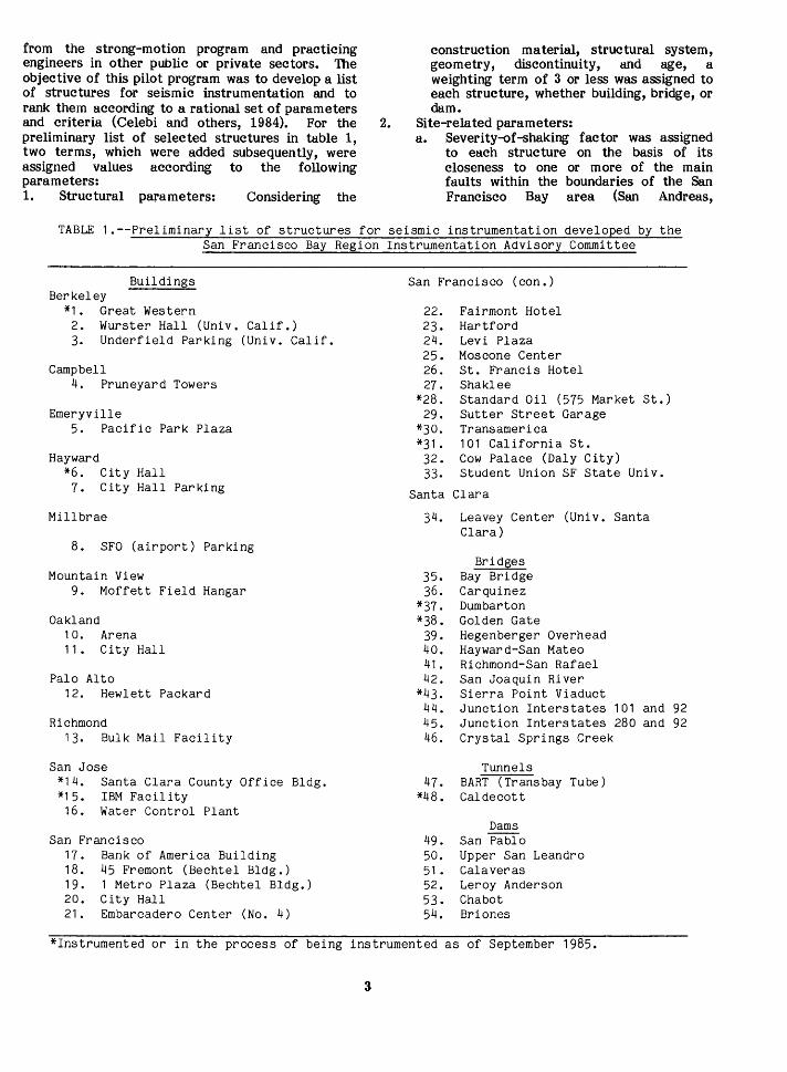
Page Table 1. Preliminary list of structures for seismic instrumentation developed

by the San Francisco Bay Region Instrumentation Advisory Committee--- 3 2. Frequencies of vibrational modes, Great Western Savings Building,

Berkeley, California-------------------------------------------------14 Dl. Suggested instrumentation for suspension span between Yerba Buena

Island and San Francisco---------------------------------------------34 D2. Suggested instrumentation for cantilevered truss span between

Yerba Buena Island and Oakland---------------------------------------35

Any use of trade names and trademarks in this publication is for descriptive purposes only and does not constitute endorsement by the

U.S. Geological Survey.

IV

Integrated Instrumentation Plan for Assessing the Seismic Response of Structures-

A Review of the Current USGS Program

By Mehmet Celebi, Erdal Safak, A. Gerald Brady, Richard Maley, and Vahid Sotoudeh

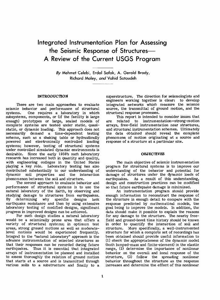
INTRODUCTION

There are two main approaches to evaluate seismic behavior and performance of structural systems. One requires a laboratory in which subsystems, components, or (if the facility is large enough) prototypes or large, scaled models of complete systems are tested under static, quasi­static, or dynamic loading. This approach does not necessarily demand a time-dependent testing scheme, such as a shaking table or hydraulically powered and electronically controlled loading systems; however, testing of structural systems under controlled simulated dynamic environments is desirable. Since the early 1950's such laboratory research has increased both in quantity and quality, with engineering colleges in the United States playing a key role. Laboratory testing has also contributed substantially to our understanding of dynamic soil properties and the interaction phenomenon between the soil and structure.

The second approach to evaluate behavior and performance of structural systems is to use the natural laboratory of the Earth, by observing and studying damage to structures from earthquakes. By determining why specific designs lack earthquake resistance and then by using extensive laboratory testing of modified designs, significant progress in improved designs can be achieved.

For such design studies a natural laboratory would be a seismically prone area that offers a variety of structural systems; in optimum test areas, strong ground motions as well as moderate­level motions would be experienced frequently. Integral to the "natural labor a tory" approach is the advance instrumentation of selected structures so that their responses can be recorded during future earthquakes. Thus it is essential that integrated arrays of instrumentation be planned and installed to assess thoroughly the relation of ground motion that starts at a source and is transmitted through various soils to a substructure and finally to a

1

superstructure. The direction for seismologists and engineers working together is clear: to develop integrated networks which measure the seismic source, the transmittal of ground motion, and the structural response processes.

This report is intended to consider issues that are related to instrumentation-strong-motion arrays, free-field instrumentation near structures, and structural instrumentation schemes. Ultimately the data obtained should reveal the complete phenomena of motion originating at a source and response of a structure at a particular site.

OBJECTIVES

The main objective of seismic instrumentation program for structural systems is to improve our understanding of the behavior and potential for damage of structures under the dynamic loads of earthquakes. As a result of this understanding, design and construction practices can be modified so that future earthquake damage is minimized.

An instrumentation program should provide enough information to reconstruct the response of the structure in enough detail to compare with the response predicted by mathematical models, the goal being to improve the models. In addition, the data should make it possible to explain the reasons for any damage to the structure. The nearby free­field and ground-level time history should be known in order to quantify the interaction of soil and structure. More specifically, a well-instrumented structure for which a complete set of recordings has been obtained should provide useful information to (1) check the appropriateness of the dynamic model (both lumped-mass and finite-element) in the elastic range, (2) determine the importance of nonlinear behavior on the overall and local response of the structure, (3) follow the spreading nonlinear behavior throughout the structure as the response increases and determine the effect of this nonlinear

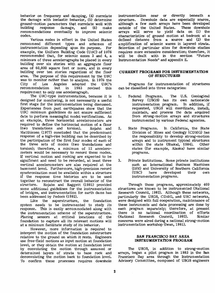
behavior on frequency and damping, (4) correlate the damage with inelastic behavior, (5) determine ground-motion parameters th~t correlate well with building response damage, and (6) make recommendations eventually to improve seismic codes.

Various codes in effect in the United States recommend different types and schemes of instrumentation depending upon its purpose. For example, the Uniform Building Code (UBC) of 1976 recommended that, for seismic zones 3 and 4, a minimum of three accelerographs be placed in every building over six stories with an aggregate floor area of 60,000 square feet or more, and in every building over ten stories regardless of the floor area. The purpose of this requirement by the UBC was to monitor rather than to analyze. In 1976 the City of Los Angeles adopted the UBC's recommendation but in 1983 revised this requirement to only one accelerograph.

The UBC-type instrumentation, because it is designed for monitoring, is not necessarily a useful first stage for the instrumentation being discussed. Experiences from past earthquakes show that the UBC minimum guidelines do not ensure sufficient data to perform meaningful model verifications. As an example, three horizontal accelerometers are required to define the horizontal motion of a floor (two translations and torsion). Rojahn and Matthiesen (1977) concluded that the predominant response of a high-rise building can be described by the participation of the first four modes of each of the three sets of modes (two translations and torsion); therefore, a minimum of 12 accelero­meters would be necessary to record these modes. If vertical motion and rocking are expected to be significant and need to be recorded, at least three vertical accelerometers are also required at the basement level. Furthermore, high-precision record synchronization must be available within a structure if the response time histories are to be used together to reconstruct the overall behavior of the structure. Rojahn and Raggett (1981) provided some additional guidelines for the instrumentation of bridges, and instrumentation for earth dams has been addressed by Fedock (1982).

Like the superstructure, the foundation system needs to be instrumented to study its response. This is easily accommodated along with the instrumentation scheme of the superstructure. Placing sensors at critical locations of the foundation to capture all its relevant motions will at a minimum facilitate study of its behavior.

However, more information is required to interpret the motion of the foundation substructure relative to the ground on which it rests. Engineers use free-field motions as input motion at foundation level, or they obtain the motion at foundation level by convoluting the motion through assumed or determined layers of strata to base rock and deconvoluting the motion back to foundation level. To confirm these processes requires downhole

2

instrumentation near or directly beneath a structure. Downhole data are especially scarce, although a few such arrays have been developed outside of the United States. These downhole arrays will serve to yield data on (1) the characteristics of ground motion at bedrock at a defined distance from a source and (2) the amplification of seismic waves in layered strata. Selection of particular sites for downhole studies requires more extensive consideration; therefore, it will be dealt with in the section "Future Instrumentation Needs" and appendix E.

CURRENT PROGRAMS FOR INSfRUMENTATION OF SfRUCTURF.S

Programs for instrumentation of structures can be classified into three categories:

1. Federal Programs. The U.S. Geological Survey (USGS) has its own nationwide instrumentation program. In addition, if requested, USGS will coordinate, install, maintain, and process the data acquired from strong-motion arrays and structures instrumented by various Federal agencies.

2. State Programs. In California, the State Division of Mines and Geology (CDMG) has the responsibility to develop strong-motion arrays and to instrument typical structures within the state (Shakal, 1984). Other states (for example, Alaska) have similar programs.

3. Private Institutions. Some private institutions such as International Business Machines (IBM) and University of Southern California (USC) have developed their own instrumentation programs.

Through these programs, approximately 400 structures are known to be instrumented (National Research Council, 1982). Although these networks, particularly the USGS, CDMG, and USC networks, were designed with full cooperation, maintenance of these instruments and data processing are done by each program separately; therefore, at present there is no national coordination of efforts (National Research Council, 1982). Similar concerns were aired during a national strong-motion instrumentation workshop (Iwan, 1981).

SAN FRANCISCO BAY AREA INSfRUMENTATION PROGRAM

The USGS, in addition to strong-motion arrays, began a pilot program in 1983 in the San Francisco Bay area through the Instrumentation Advisory Committee, composed of USGS engineers

from the strong-motion program and practicing engineers in other public or private sectors. The objective of this pilot program was to develop a list of structures for seismic instrumentation and to rank them according to a rational set of parameters and criteria (Celebi and others, 1984). For the preliminary list of selected structures in table 1, two terms, which were added subsequently, were assigned values according to the following parameters: 1. Structural parameters: Considering the

2.

construction material, structural system, geometry, discontinuity, and age, a weighting term of 3 or less was assigned to each structure, whether building, bridge, or dam.

Site-related parameters: a. Severity-of-shaking factor was assigned

to each structure on the basis of its closeness to one or more of the main faults within the boundaries of the San Francisco Bay area (San Andreas,

TABLE 1.--Preliminary list of structures for seismic instrumentation developed by the San Francisco Bay Region Instrumentation Advisory Committee

Buildings Berkeley

*1. Great Western 2. Wurster Hall (Univ. Calif.) 3. Underfield Parking (Univ. Calif.

Campbell 4. Pruneyard Towers

Emeryville 5. Pacific Park Plaza

Hayward *6. City Hall

7. City Hall Parking

Millbrae

8. SFO (airport) Parking

Mountain View 9. Moffett Field Hangar

Oakland 1 o. 11.

Arena City Hall

Palo Alto 12. Hewlett Packard

Richmond 13. Bulk Mail Facility

San Jose *14. Santa Clara County Office Bldg. *15. IBM Facility

16. Water Control Plant

San Francisco 17. Bank of America Building 18. 45 Fremont (Bechtel Bldg.) 19. 1 Metro Plaza (Bechtel Bldg.) 20. City Hall 21. Embarcadero Center (No. 4)

San Francisco (con.)

22. Fairmont Hotel 23. Hartford 24. Levi Plaza 25. Moscone Center 26. St. Francis Hotel 27. Shaklee

*28. Standard Oil (575 Market St.) 29. Sutter Street Garage

*30. Transamerica *31. 101 California St. 32. Cow Palace (Daly City) 33. Student Union SF State Univ.

Santa Clara

34. Leavey Center (Univ. Santa Clara)

35. 36.

*37. *38.

39. 40. 41. 42.

*43. 44. 45. 46.

47. *48.

49. 50. 51. 52. 53. 54.

Bridges Bay Bridge Carquinez Dum barton Golden Gate Hegenberger Overhead Hayward-San Mateo Richmond-San Rafael San Joaquin River Sierra Point Viaduct Junction Interstates 101 and 92 Junction Interstates 280 and 92 Crystal Springs Creek

Tunnels BART (Trans bay Tube) Caldecott

Dams San Pablo Upper San Leandro Calaveras Leroy Anderson Chabot Briones

*Instrumented or in the process of being instrumented as of September 1985.

3

Hayward, and Calaveras faults). A map prepared for this purpose was used to obtain these factors (Borcherdt and others, 1975).

b. Probability of a large earthquake (M = 6.5 or 7) occurring on the fault(s) within the next 30 years was obtained. A study made for this purpose (Lindh, 1983) was used to obtain the probabilities.

c. Expected value of strong shaking at the site was then determined as the product of a and b. This product was then multiplied by a factor to upgrade the maximum expected value of strong­shaking factor to 3, which was the maximum value used for the structural parameter. Thus the structural parameter and site-related parameters are given equal weights.

The final product of the developed methodology is provided in table 1, which presents different structures in different regions of the San Francisco Bay area according to their priority for instrumentation. Some of the structures have already been or are in the process of being in­strumented.

The activities associated with the USGS strong-motion instrumentation program are supervised by the Chief of the Branch of Engineering Seismology and Geology (ESG), a unit within the Office of Earthquakes, Volcanoes, and Engineering. Associated with the branch is the Instrumentation Advisory Committee (lAC). After the lAC formulates its recommendations, they are transmitted to the Branch Chief and to the engineering staff of ESG through technical and planning reports for implementation (fig. 1). The engineering staff in turn obtains instrumentation permits for selected structures, gathers information relative to the project including structural plans and design and model information, and directs structural evaluation and if necessary performs ambient response studies. This integrated set of data is then used as a basis for determining transducer locations that will adequately define the response of the structure during a strong earthquake. The actual selection of measurement points in the structure is carried out with the members of the strong-motion section installation team. Mter the sensor loca­tions have been agreed upon by the engineering staff, the installation team, a representative of the owner of the structure, and an electrical contractor are called in to plan placement of the data cable. The installation team works with the contractor during this phase and subsequently calibrates and installs sensors and recording systems. A final step is a complete documentation of each transducer location and orientation, characteristics of total system response, and any peculiarities of the instrumentation or access to required sites. A

4

summary description of the completed system is then available to members of ESG and to other interested engineers and scientists. These steps are described in more detail in the following section.

STEPS IN INSTRUMEN'ftNG A STRUCTURE

Once it is decided to instrument a structure, a series of studies, deductions, and decisions follow. It is important to optimize the instrumentation schemes from the points of view of both cost and required data. Too few instruments do not yield sufficient data to record the performance of a structure during an earthquake. This has been the case for many buildings in the past. As mentioned above, even now the Uniform Building Code recom­mends only three accelerographs for buildings meeting certain qualifying characteristics, although the UBC does not intend that a detailed structural analysis be possible from its recommended instrumentation. Rojahn and Matthiesen (1977) and Hart and Rojahn (1979) have made studies related to instrumentation needs of a structure. A detailed study of how to determine the quantity and locations of sensors to obtain necessary data of structural performance during earthquakes is pre sen ted in appendix A, which is directly from Erdal Safak (written commun., 1985).

In order to optimize the instrumentation it is important to study the expected dynamic behavior of the structure. The preliminary studies include the following steps:

(1) study of available design and analysis information after permission for instrumenting is granted by the owner,

(2) site visit, and (3) required analytical studies and tests.

It is not automatic for an owner of a structure to grant permission for an outside agency to install instruments. Some owners willingly cooperate; others fear that there may be some hidden objectives that will cause them financial losses. In general, however, per mission is granted once the objectives of the program are explained fully. This in turn makes it possible to obtain structural information. Ideally, the following information, if available, will be required: relevant blueprints and design calculations, dynamic analysis (mode shapes and frequencies), forced-vibration test results, and ambient-vibration test results.

Seldom is all this information available for any structure. For the structure to be instrumented, a minimum requirement is that ambient-vibration tests be performed to obtain mode shapes and frequencies. If forced-vibration tests have been performed to obtain the mode shapes and frequencies, ambient vibration tests are not normally needed.

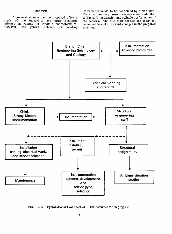
Site Visit

A general scheme can be prepared after a study of the blueprints and other available information related to dynamic characteristics. However, the general scheme for locating

instruments needs to be confirmed by a site visit. The structure may present various constraints that affect safe installation and reliable performance of the sensors. The site visit enables the technical personnel to make relevant changes in the prepared schemes.

Branch Chief, Engineering Seismology

and Geology ..

Technical planning and reports

Instrumentation Advisory Committee

Chief, Strong Motion

Instrumentation ---•1 Documentation 1•---

Structural engineering

staff

1•--------- r---lnst-rume-nt ~•------- -1 lnsta llation

cabling, electrical work, and sensor selection

1 Maintenance

installation permit

l Instrumentation

scheme, development, and

sensor (type) selection

Structural design study

1 Ambient -vibration

studies

FIGURE 1.-0rganizational flow chart of USGS instrumentation program.

5

Ambient-Vibration Tests

Preliminary analytical studies usually give a fairly accurate view of the structure's expected dynamic behavior. Using this information, the next step is to per form an ambient-vibration test on the structure. The test is done fairly quickly using portable recorders at three to five locations that are expected (from analytical studies or other information) to have maximum amplitudes during lower vibrational modes.

The ambient-vibration data are processed using the procedure given in appendix B. The structural parameters (natural frequencies, damping, and mode shapes) are calculated through a random-vibration approach.

The importance of ambient-vibration analysis is that it gives the elastic properties of the structure. During a strong earthquake the structure may experience nonlinear behavior; thus, if the parameters of linear behavior are known beforehand, it is easier to analyze the nonlinear behavior.

Forced-Vibration Test

A forced-vibration test is more difficult than an ambient-vibration test. The required equipment (vibration generator with control consoles, weights, recorders, accelerometers, and cables) is heavier, and the test takes longer than the ambient-vibration test. Furthermore, state-of-the-art vibration generators do not necessarily have the capability to excite to resonance all significant modes of all structures. A general description and some of the many references on forced-vibration testing is provided in appendix C.

Dynamic Analysis

If a dynamic analysis was not prepared by the designers of a structure or the information is unavailable, then a simplified finite-element model is developed to obtain the elastic dynamic characteristics. This is performed with any one of the several tested computer programs available (such as SAP, STARDYNE, ANSYS, and STRUDL).

Installation of Instruments

After approximate sensor locations are chosen, a USGS technician and the owner's representative review each site to determine exact sensor locations satisfactory to both parties. In general, final criteria must consider long-term accessibility, potential interference with the occupant's space, placement of data cable runs, and aesthetic requirements of the owner.

Next the USGS technician inspects the entire structural scheme with an electrical contractor who

6

will install the data cable and terminal boxes at each sensor site. Actual cabling by the contractor is monitored by the USGS and the owner's representative to be sure the cable is installed as desired and that all building code regulations are followed.

The cable-termination box is prepared in the USGS shop and includes data and calibration circuits, batteries, battery chargers, radio circuit board or time-code generator, digital-event counter, and electronic test points. This box, normally mounted on the wall above the recorder, contains external connectors for all data channels so that signals may be amplified and used to record the ambient response of the structure at any time. The recorder location is selected on the basis of security, typically in a telephone or electrical switch room, and in some circumstances is enclosed with separate fencing in an open area.

The instrumentation undergoes a preliminary calibration in the strong-motion laboratory and is then installed in the structure with appropriate test procedures including a static tilt sensitivity test for each component and determination of direction of motion for upward trace deflection on the record. These data are permanently stored on film as part of the system description. Other documentation includes precise sensor location, period and damping of each unit, location of cable runs, access information, and circuit diagrams.

Maintenance

It is essential to have periodic and consistent maintenance of instruments in order to have a successful program. Therefore, routine maintenance is conducted every 3 months initially and may be extended to every 12 months if circumstances and experience so allow. This maintenance includes the following:

1. Remote calibration of period and damping. 2. Inspection of battery terminals, load voltage,

and charge rate (batteries are replaced every 3 years).

3. Check of lamp intensity and voltage and the trace positions on the recording film.

4. Measurement of threshold of triggering system and length of recording cycle.

5. Check of film take-up and supply (the film is replaced each year).

6. Inspection for operation and synchronization of the WWVB radio receiver or time-code generator.

As a final maintenance procedure, a calibration record is returned for developing and then examined for the desired characteristics. All inspection procedures are recorded in duplicate with one copy left at the recorder site and the second in the permanent station file at the laboratory.

Instrumentation for Structural Response Studies

Instrumentation intended for strong-motion structural-response studies can be broadly classified under two categories according to recording techniques: (1) analog recording on 7-in. and 70-mm film, recording 12 and 3 channels, respectively, of data, and (2) digital recording on magnetic tape cassette at 100 or 200 samples per second, recording data in multiples of three channels per unit.

The use of digital recording systems in structures, begun by the USGS in 1975, has proved somewhat less than satisfactory, although new digital recorders are considerably improved. The development over many years of highly reliable, less costly analog recorders has led to their installation in most instrumented structures. Since this discussion refers only to the recording mode and not to the sensors or manner of data transmission, the collection of data in an analog mode is not necessarily a permanent feature in structural studies; if digital recorders achieve the same high reliability and competitive prices, they will be installed in new structures and could replace any outdated recorders presently in use.

The analog recorder usually installed for structural-response studies is the Kinemetrics CRA-1 capable of recording 12 or 13 channels of data on a single 7-in. film. In this system, incoming signals are directly transmitted to 150-Hz galvanometers, which in turn deflect a light beam across the moving film strip. The instrument, triggered by a vertical starter with a nominal threshold of 0.01 .[ between 1 and 10 Hz, has a total recording time of 25 minutes. The recorder continues to operate for approximately 20 seconds (shop adjustable) after the last occurrence of vertical ground motion exceeding the triggering threshold, in order to record the earthquake fully. An internal clock impresses half­second time marks on the edge of the film. A second timing system, installed as an optional feature by the USGS, puts real time on the opposite edge of the film from an internal time-code generator or by using a WWVB radio code signal. In the latter case the instrument must operate for a minimum of 60 seconds in order to accommodate the entire WWVB code. Power is supplied by float­charged batteries located in a nearby battery box. A rotary key switch provides for periodic testing of natural frequency and damping of the remotely located sensors.

Sensors usually installed in the USGS program are 5Q-Hz, 0. 7 critically damped Kinemetrics force­balance accelerometer models FBA-11 and FBA-13 (respectively uniaxial and triaxial transducers). The accelerometers are bolted to the building frame or floor, and sensed data are transmitted to the central recording location by shielded cable. In some applications Terra Technology SA-102 servo

7

accelerometers with similar response character­istics have been used.

Triaxial self -contained accelerographs are often installed in conjunction with the remote­sensor system either to record free-field ground motions or to supplement the structural instrumentation when more than 12 chtJ.nnels are required. This instrument, generally a Kinemetrics SMA-1, records data optically onto 70-mm film from 25-Hz flexure-type accelerometers. The SMA-1 has the same trigger system, recording capability, and real time options as described for the CRA-1. Some Teledyne RFT-250 accelerographs, with characteristics similar to the SMA-1, are used at free-field sites after extensive modification by the USGS.

The approximate cost of instrumenting a typical building (defined as a 25-story structure) with a 12 channel CRA-1, a free field SMA-1, and all previously described options is approximately $40,000 excluding USGS salary costs. The use of digital recording would increase this figure by $14,000.

Data Processing

Records are processed according to the descriptions in the computer program AG RAM developed by Converse (1984). Briefly, the steps are as follows: 1. The film records are digitized at a commercial

firm on a trace-following, computer-controlled laser scanner. Unequal time spacing, at an average of 600 samples per second, is used.

2. The separately digitized, 10-second frames are reassembled using specially inserted vertical lines; each vertical line is digitized twice, once in each adjacent frame.

3. The uncorrected data are prepared by subtracting out the reference traces, using the time marks for the x-coordinates, and subtracting the average value. Plots of the uncorrected data are prepared.

4. The data from both film and digital recordings are then passed through a correction algorithm that applies a high-frequency filter (50 Hz), instrument corrections, and decimation to 200 samples per second. A low-frequency high-pass Butterworth filter removes all periods longer than a predetermined period from the data. This period is chosen after consideration of the strong-motion duration of the records, any distortion during pre-event memory on the digitals, displacements calculated at specific sites, and displacements of adjacent film and digital recordings at specific sites. Plots of the corrected acceleration, velocity, and displacements for the three components of each recording are prepared.

5. Response spectra are calculated for periods up to the long-period limit. Linear plots of relative-velocity response spectra and the log-

log tripartite plots of pseudo-velocity response are prepared.

6. Fourier amplitude spectra, calculated by fast Fourier transform, are presented on linear axes and log-log axes.

EXAMPLES OF STRUCTURAL INSTRUMENTA'llON SCHEMES

Pacific Park Plaza, Emeryville

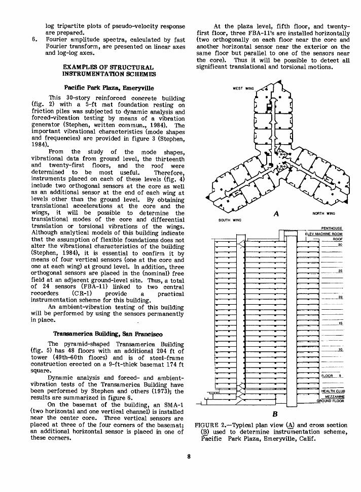
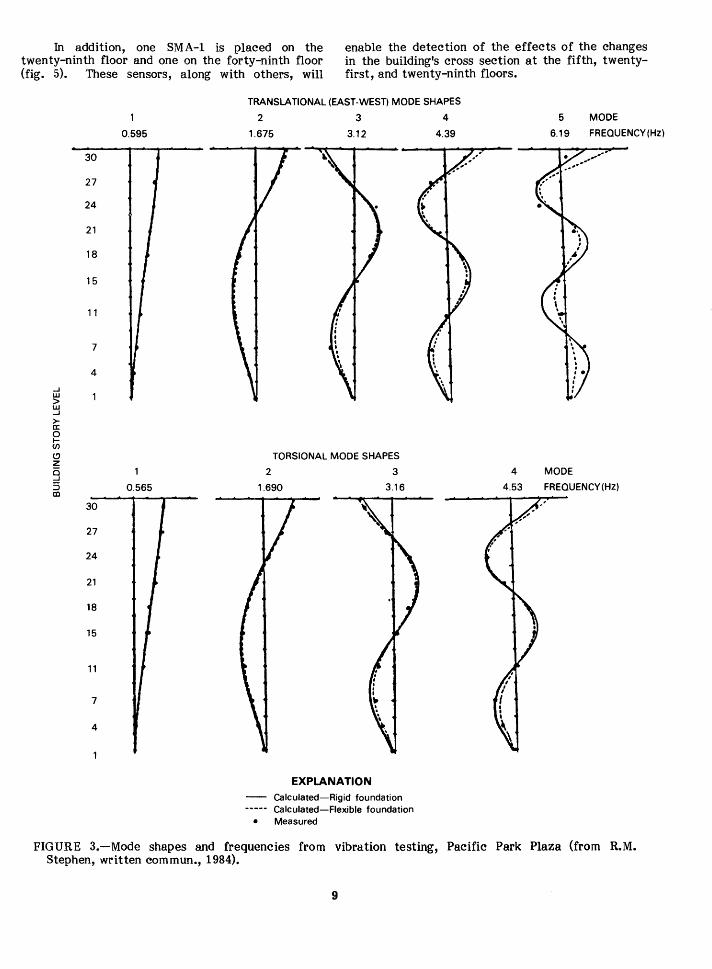
This 30-story reinforced concrete building (fig. 2) with a 5-ft mat foundation resting on friction piles was subjected to dynamic analysis and forced-vibration testing by means of a vibration generator (Stephen, written commun., 1984). The important vibrational characteristics (mode shapes and frequencies) are provided in figure 3 (Stephen, 1984).

From the study of the mode shapes, vibrational data from ground level, the thirteenth and twenty-first floors, and the roof were determined to be most useful. Therefore instruments placed on each of these levels (fig. 4) include two orthogonal sensors at the core as well as an additional sensor at the end of each wing at levels other than the ground level. By obtaining translational accelerations at the core and the wings, it will be possible to determine the translational modes of the core and differential translation or torsional vibrations of the wings. Although analytical models of this building indicate that the assumption of flexible foundations does not alter the vibrational characteristics of the building (Stephen, 1984), it is essential to confirm it by means of four vertical sensors (one at the core and one at each wing) at ground level. In addition, three orthogonal sensors are placed in the (nominal) free field at an adjacent ground-level site. Thus, a total of 24 sensors (FBA-11) linked to two central recorders (CR-1) provide a practical instrumentation scheme for this building.

An ambient-vibration testing of this building will be performed by using the sensors permanently in place.

Transamerica Building, San Francisco

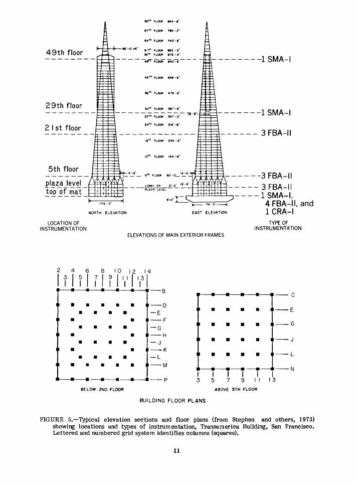
The pyramid-shaped Transamerica Building (fig. 5) has 48 floors with an additional 204 ft of tower (49th-60th floors) and is of steel-frame construction erected on a 9-ft-thick basemat 174ft square.

Dynamic analysis and forced- and ambient­vibration tests of the Transamerica Building have been performed by Stephen and others (1973); the results are summarized in figure 6.

On the basemat of the building, an SMA-1 (two horizontal and one vertical channel) is installed near the center core. Three vertical sensors are placed at three of the four corners of the basemat; an additional horizontal sensor is placed in one of these corners.

8

At the plaza level, fifth floor, and twenty­first floor, three FBA-11's are installed horizontally (two orthogonally on each floor near the core and another horizontal sensor near the exterior on the same floor but parallel to one of the sensors near the core). Thus it will be possible to detect all significant translational and torsional motions.

SOUTH WING

r--

r<

-

1- -

,- - -,- - -

- -K

-=L r-.., I

r - -<- --Ll L_-·

I fr--

-- --

- -

----

I J.-- .....__

B

ELEV MA

I -

--

--

PENTHOUSE

CHINE ROOM

~ 30

--~

___ 1.§._

__ _!Q_

FLOOR ___ 5 __

GA

HEALTH CLUB

MEZZANINE OUNO FLOOR

FIGURE 2.-Typical plan view (A) and cross section (B) used to determine instrumentation scheme, Pacific Park Plaza, Emeryville, Calif.

In addition, one SMA-1 is placed on the twenty-ninth floor and one on the forty-ninth floor (fig. 5). These sensors, along with others, will

enable the detection of the effects of the changes in the building's cross section at the fifth, twenty­first, and twenty-ninth floors.

0.595

30

27

24

21

18

15

11

7

4

_J w > w _J

>-a: 0 t-en (!) z i5 _J

5 0.565 CD

30

27

24

21

18

15

11

7

4

TRANSLATIONAL (EAST-WEST) MODE SHAPES

2 3 4

1.675 3.12 4.39

TORSIONAL MODE SHAPES

2 3

1.690 3.16

EXPLANATION Calculated-Rigid foundation Calculated-Flexible foundation

• Measured

4

4.53

5 MODE

6.19 FREQUENCY (Hz)

MODE

FREQUENCY (HZ)

FIGURE 3.-Mode shapes and frequencies from vibration testing, Pacific Park Plaza (from R.M. Stephen, written commun., 1984).

9

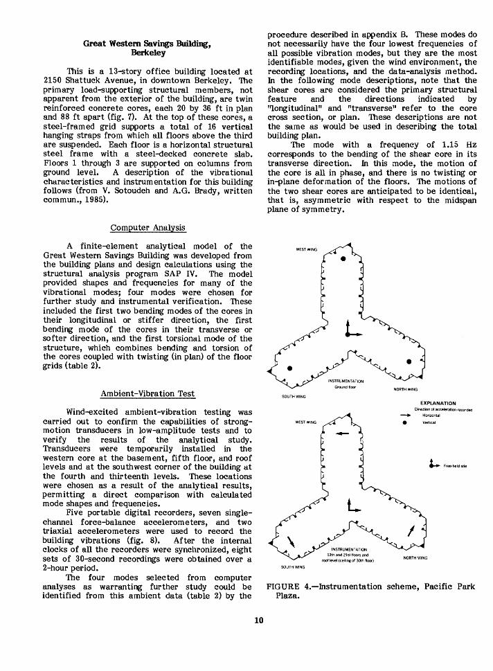
Great Westem Savings Building, Berkeley

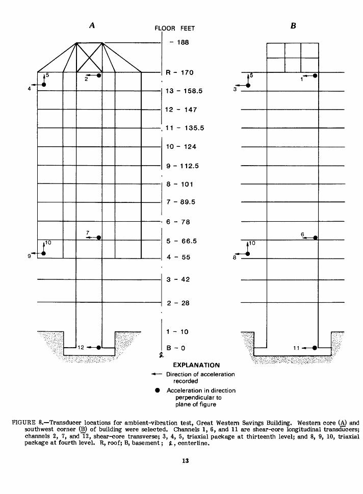
This is a 13-story office building located at 2150 Shattuck Avenue, in downtown Berkeley. The primary load-supporting structural members, not apparent from the exterior of the building, are twin reinforced concrete cores, each 20 by 36 ft in plan and 88 ft apart (fig. 7). At the top of these cores, a steel-framed grid supports a total of 16 vertical hanging straps from which all floors above the third are suspended. Each floor is a horizontal structural steel frame with a steel-decked concrete slab. Floors 1 through 3 are supported on columns from ground level. A description of the vibrational characteristics and instrumentation for this building follows (from V. Sotoudeh and A. G. Brady, written commun., 1985).

Computer Analysis

A finite-element analytical model of the Great Western Savings Building was developed from the building plans and design calculations using the structural analysis program SAP IV. The model provided shapes and frequencies for many of the vibrational modes; four modes were chosen for further study and instrumental verification. These included the first two bending modes of the cores in their longitudinal or stiffer direction, the first bending mode of the cores in their transverse or softer direction, and the first torsional mode of the structure, which combines bending and torsion of the cores coupled with twisting (in plan) of the floor grids (table 2).

Ambient-Vibration Test

Wind-excited ambient-vibration testing was carried out to confirm the capabilities of strong­motion transducers in low-amplitude tests and to verify the results of the analytical study. Transducers were temporarily installed in the western core at the basement, fifth floor, and roof levels and at the southwest corner of the building at the fourth and thirteenth levels. These locations were chosen as a result of the analytical results, permitting a direct comparison with calculated mode shapes and frequencies.

Five portable digital recorders, seven single­channel force-balance accelerometers, and two triaxial accelerometers were used to record the building vibrations (fig. 8). After the internal clocks of all the recorders were synchronized, eight sets of 30-second recordings were obtained over a 2-hour period.

The four modes selected from computer analyses as warranting further study could be identified from this ambient data (table 2) by the

10

procedure described in appendix B. These modes do not necessarily have the four lowest frequencies of all possible vibration modes, but they are the most identifiable modes, given the wind environment, the recording locations, and the data-analysis method. In the following mode descriptions, note that the shear cores are considered the primary structural feature and the directions indicated by "longitudinal" and "transverse" refer to the core cross section, or plan. These descriptions are not the same as would be used in describing the total building plan.

The mode with a frequency of 1.15 Hz corresponds to the bending of the shear core in its transverse direction. In this mode, the motion of the core is all in phase, and there is no twisting or in-plane deformation of the floors. The motions of the two shear cores are anticipated to be identical, that is, asymmetric with respect to the midspan plane of symmetry.

SOUTH WING

EXPLANATION Direction of acceleratiOn recorded

1... Free-f1eld site

SOUTH WING

FIGURE 4.-Instrumentation scheme, Pacific Park Plaza.

49th floor II t 11 FLOOR •t3' • 2" !101h FLOOR .-T&'- 4"

- - - - --..-'" 'Loci! .-.o-:a··- - - - - - - - - - - -1 SMA -I

29th floor

2 I st floor --------~~------------ 8§~------ 3 FBA-11

J:i::: 11 1 ~ FLOOII 25!>'-15" a=

LOCATION OF INSTRUMENTATION

NORTH ELEVATION

2 4 6 8 10

EAST ELEVATION

ELEVATIONS OF MAIN EXTERIOR FRAMES

12 14

TYPE OF INSTRUMENTATION

I T I I I I I i 1111

1113

1 -s --c

• • • • -D

• • • • -E • • • • --E

• -F

• • • • • • • --G • -G

• -H

• • • • -J • • • • --J

• -K

• • • • -L • • • • --L

• • • • -M -----.---------. --N I I I I I I ---- • • -P 3 5 7 9 I I 13

BELOW 2ND FLOOR ABOVE 5TH FLOOR

BUILDING FLOOR PLANS

FIGURE 5.-Typical elevation sections and floor plans (from Stephen and others, 1973) showing locations and types of instrumentation, Transamerica Building, San Francisco. Lettered and numbered grid system identifies columns (squares).

11

FLOOR

60 57 54

42

36

30

24

18

12

NORTH-SOUTH EAST-WEST

First mode: f = 0.345 Hz

FLOOR FLOOR

•

NORTH-SOUTH EAST-WEST

Second mode: f = 0.635 Hz

EXPLANATION Calculated Forced-vibration test

• Ambient-vibration test

NORTH-SOUTH EAST-WEST

Third mode: f = 1.17 Hz (N-S) f = 1.13 Hz (E-W)

FIGURE 6.-Mode shapes and frequencies from vibration testing, Transamerica Building (from Stephen and others, 1973). Horizontal lines correspond to floor levels in figure 5.

~B .. u1ldmg North north

I

~ _L __ j_l_-L ___ J ............ ~~ f I I I I [ I I I lb"o"o 1 i ,--r-----r- ---------r-------r--:--1------l- "='" oore l------1-~ ~ -h J

~ ----+- +----+-l-+--- ~~~~ l Core I ,,_ __ 3 __ ~ Hanging straps ....£-___ ....,.

longitudinal I direction I

FIGURE 7.-Floor plan of Great Western Savings Building, Berkeley, Calif. Grid system identifies vertical hanging straps from which all floors above the third are suspended.

12

A

/1 X ~ 4

us re -

~

.-9 ~r

... :ryiEw~ ::::}~h· ., .•..

;--~\~~ ~ 12--------:-.

. :: <:_{ o;;:c·;·<·~;:~:::}.::::'':·,· .\-;. >

FLOOR FEET B

- 188

R- 170

13- 158.5

l5 1----3_j

12- 147

11 - 135.5

10- 124

9- 112.5

8 - 101

7- 89.5

6- 78

5 - 66.5

4- 55

~ 10

a_j

3- 42

2- 28

1 - 10

~ :::.' 11 ------=:;/ B-0

1 EXPLANATION

~;~::;_{\ .:·~· ~ ;::;:F:~~::\_:·.~· ,. :::.::::;•;:;.;:._,.,:· .. ·.:-; .. , .. _,.,, ..•..

...-- Direction of acceleration recorded

e Acceleration in direction perpendicular to plane of figure

~ r.f:_;(

n ,::).'~{:•.

FIGURE B.-Transducer locations for ambient-vibration test, Great Western Savings Building. Western core (A) and southwest corner (B) of building were selected. Channels 1, 6, and 11 are shear-core longitudinal transducers; channels 2, 7, and 12, shear-core transverse; 3, 4, 5, triaxial package at thirteenth level; and 8, 9, 10, triaxial package at fourth level. R, roof; B, basement; t, centerline.

13

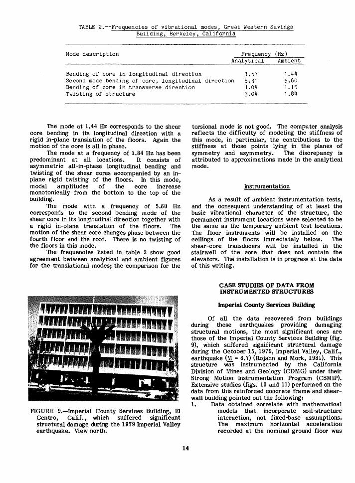
TABLE 2.--Frequencies of vibrational modes, Great Western Savings Building, Berkeley, California

Mode description Frequency (Hz) Analytical Ambient

Bending of core in longitudinal direction 1. 57 5.31 1.04 3.04

1. 44 5.60 1. 15 1.84

Second mode bending of core, longitudinal direction Bending of core in transverse direction Twisting of structure

The mode at 1.44 Hz corresponds to the shear core bending in its longitudinal direction with a rigid in-plane translation of the floors. Again the motion of the core is all in phase.

The mode at a frequency of 1.84 Hz has been predominant at all locations. It consists of asymmetric ail-in-phase longitudinal bending and twisting of the shear cores accompanied by an in­plane rigid twisting of the floors. In this mode, modal amplitudes of the core increase monotonically from the bottom to the top of the building.

The mode with a frequency of 5.60 Hz corresponds to the second bending mode of the shear core in its longitudinal direction together with a rigid in-plane translation of the floors. The motion of the shear core changes phase between the fourth floor and the roof. There is no twisting of the floors in this mode.

The frequencies listed in table 2 show good agreement between analytical and ambient figures for the translational modes; the comparison for the

FIGURE 9.-lmperial County Services Building, El Centro, Calif., which suffered significant structural damage during the 1979 Imperial Valley earthquake. View north.

14

torsional mode is not good. The computer analysis reflects the difficulty of modeling the stiffness of this mode, in particular, the contributions to the stiffness at those points lying in the planes of symmetry and asymmetry. The discrepancy is attributed to approximations made in the analytical mode.

Instrumentation

As a result of ambient instrumentation tests, and the consequent understanding of at least the basic vibrational character of the structure, the permanent instrument locations were selected to be the same as the temporary ambient test locations. The floor instruments will be installed on the ceilings of the floors immediately below. The shear-core transducers will be installed in the stairwell of the core that does not contain the elevators. The installation is in progress at the date of this writing.

CASE STUDIES OF DATA FROM INSTRUMENTED STRUCTURES

Imperial County Services Building

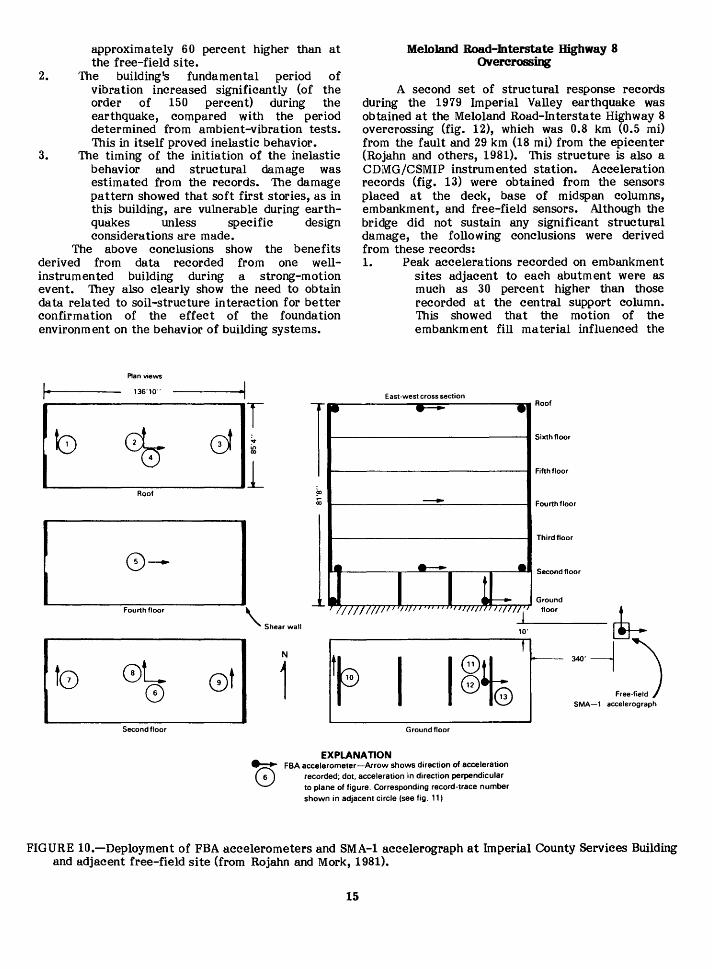
Of all the data recovered from buildings during those earthquakes providing damaging. structural motions, the most significant ones are those of the Imperial County Services Building (fig. 9), which suffered significant structural damage during the October 15, 1979, Imperial Valley, Calif., earthquake (M = 6. 7) (Rojahn and Mork, 1981). This structure was instrumented by the California Division of Mines and Geology (CDMG) under their Strong Motion Instrumentation Program (CSMIP). Extensive studies (figs. 10 and 11) performed on the data from this reinforced concrete frame and shear­wall building pointed out the following: 1. Data obtained correlate with mathematical

models that incorporate soil-structure interaction, not fixed-base assumptions. The maximum horizontal acceleration recorded at the nominal ground floor was

approximately 60 percent higher than at the free-field site.

2. The building's fundamental period of vibration increased significantly (of the order of 150 percent) during the earthquake, compared with the period determined from ambient-vibration tests. This in itself proved inelastic behavior.

3. The timing of the initiation of the inelastic behavior and structural damage was estimated from the records. The damage pattern showed that soft first stories, as in this building, are vulnerable during earth­quakes unless specific design considerations are made.

The above conclusions show the benefits derived from data recorded from one well­instrumented building during a strong-motion event. They also clearly show the need to obtain data related to soil-structure interaction for better confirmation of the effect of the foundation environment on the behavior of building systems.

Plan views

136'10" ·I

lb T 1 ~ C2J ~ ll'l

I co

l Roof iD

a;

8---I

Fourth floor

\.Shear wall

I I

0L ' f0 I 0

N

1 Second floor

Melo1and Road-Interstate llighway 8 Overcrossing

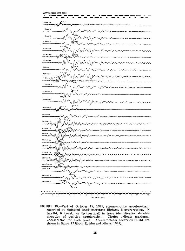
A second set of structural response records during the 1979 Imperial Valley earthquake was obtained at the Meloland Road-Interstate Highway 8 overcrossing (fig. 12), which was 0.8 km (0.5 mi) from the fault and 29 km (18 mi) from the epicenter (Rojahn and others, 1981). This structure is also a CDMG/CSMIP instrumented station. Acceleration records (fig. 13) were obtained from the sensors placed at the deck, base of midspan columns, embankment, and free-field sensors. Although the bridge did not sustain any significant structural damage, the following conclusions were derived from these records: 1. Peak accelerations recorded on embankment

sites adjacent to each abutment were as much as 30 percent higher than those recorded at the central support column. This showed that the motion of the embankment fill material influenced the

East-west cross section Roof

Sixth floor

Fifth floor

--- Fourth floor

Third floor

SMA-1 accelerograph

Ground floor

EXPLANATION FBA accelerometer-Arrow shows direction of acceleration

recorded; dot, acceleration in direction perpendicular to plane of figure. Corresponding record-trace number shown in adjacent circle (see fig. 11)

FIGURE 10.-Deployment of FBA accelerometers and SMA-1 accelerograph at Imperial County Services Building and adjacent free-field site (from Rojahn and Mork, 1981).

15

motion of the abutment. Also there was evidence of relative motion between the abutments and the surrounding fill material.

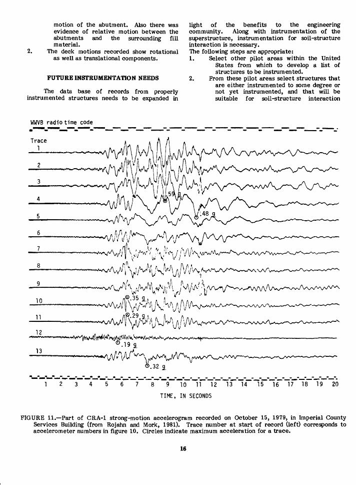
2. The deck motions recorded show rotational as well as translational components.

FUTURE INSTRUMENTATION NEEDS

The data base of records from properly instrumented structures needs to be expanded in

WWVB radio time code

light of the benefits to the engineering community. Along with instrumentation of the superstructure, instrumentation for soil-structure interaction is necessary. The following steps are appropriate: 1. Select other pilot areas within the United

States from which to develop a list of structures to be instrumented.

2. From these pilot areas select structures that are either instrumented to some degree or not yet instrumented, and that will be suitable for soil-structure interaction

_ __. --- - - - ---- __ _. ____ - - --· . - - ~ - - - -. -- - - - - - - -- -Trace

1

2

3

4

5

12

------.....·----------· . - . - - - - - - - - . - - - - - - - - - - - - - - - - - - - -, 2 3 4--s--6--7--s--9-1a111213141s161718192o

TIME, IN SECONDS

FIGURE 11.-Part of CRA-1 strong-motion accelerogram recorded on October 15, 1979, in Imperial County Services Building (from Rojahn and Mork, 1981). Trace number at start of record (left) corresponds to accelerometer numbers in figure 10. Circles indicate maximum acceleration for a trace.

16

II II

104'-0" 208'-0"

----Abu;-;e~,-·~-----.,===~-:::::-1~~--t....----===,;

Embankment toe

SECTION A-A'

(I) c ~ "0 c ::I 0 -e <ll (I)

w

EAST ELEVATION

® 20'-8" L

GG

PLAN

II II

--!~---

Abutment 3

EXPLANATION

FBA accelerometer-Arrow shows direction of accel­eration recorded; dot, acceleration in direction perpendicular to plane of figure. Corresponding record-trace number shown in adjacent circle (see fig. 13)

Note. Accelerometers 1, 2, and 4 mounted on footmg m ground vault; 10-12, 14-15, and 23-26 located m ground vault beneath ground surface; and 3, 5-9, 13, and 16-22 mounted on s1de of box g1rder supportmg roadway deck

FIGURE 12.-Deployment of FBA accelerometers at Meloland Road-Interstate Highway 8 overcossing, which is 29 km (18 mi) from epicenter of 1979 Imperial Valley earthquake (from Rojahn and others, 1981).

17

WWVB radio time code --- _ ....... ___ ._, - .. --- ----- ~ -. ~-.._.. __ TlBasel Up_ _ • -~7 ~g • • .••.

~-~·~~~~-------------------------------------2 IBaseiW

3 IDeckl W

4 (Base) N

11 ISEmbiW

12 IS Embl N

• "'~"'~ 1'\.../\r~

13(0eckiW

028

~9

---<JV'\}

141FrFidl U_:> • .J J.f~ 23 g O

48 g

~·yu.,""..t~~ ... ~----,.......--~---------------

. . . . . . . . . . . . . - - - - - - . - - - - - - - - - - - - - - - - - - - . -------~-----~-----~---~---------------0 1 2 3 4 5 6 7 8 9 10 11 12 13 14 15 16 17 18 19

TIME. IN SECONDS

FIGURE 13.-Part of October 15, 1979, strong-motion accelerogram recorded at Meloland Road-Interstate Highway 8 overcrossing. N (north), W (west), or Up (vertical) in trace identification denotes direction of positive acceleration. Circles indicate maximum acceleration for each trace. Accelerometer locations (1-26) are shown in figure 12 (from Rojahn and others, 1981).

18

studies. These ·studies would use horizontal and vertical spatially varying arrays that may include additional specific instruments for special purposes.

3. Plan in advance for instrumentation of a future building to be erected at a suitable site.

These sites should be near existing or planned ground-level arrays in seismically active regions so that data from an integrated scheme that includes the source, site soil-structure interaction, and superstructure will enable complete studies.

At present, in addition to the San Francisco Bay area, other regions with strong shaking potential, such as San Bernardino County (California), Anchorage (Alaska), and Charleston (South Carolina) are being surveyed as separate pilot areas. Still other regions (New Madrid area, Missouri) are to be surveyed in the near future. A detailed description of instrumentation needs related to soil-structure interaction is provided in appendix E.

CONCLUSIONS

This report presents the current methods and status of instrumenting structures and. discusses the benefits derived from instrumenting a structure as well as the extent to which a structure should be instrumented. It also reviews some lessons derived from well-instrumented structures in earthquakes. Our main conclusions are two:

1. It is better to instrument fewer structures with extensive instruments so that their performance can be fully recorded than to instrument many structures with minimum instruments.

2. Soil-structure interaction has to be accounted for in the mathematical models of the structures.

In line with these conclusions, a needed improvement is to provide borehole instrumentation near well-instrumented structures to obtain data on the vertical and horizontal spatial variation of earthquake motion along the immediate periphery of the buildings. The information derived certainly should answer questions related to soil-structure interaction, horizontal and spatial variation of earthquake motions, and building-to-building interaction where applicable.

REFERENCES CITED

Borcherdt, R.D., Gibbs, J.F., and Lajoie, K.R., 1975, Maximum earthquake intensity predicted for large earthquakes: U.S. Geological Survey Miscellaneous Field Studies Map MF-709, scale 1:125,000, 3 sheets.

19

Celebi, M., and others, 1984, Report on recommended list of structures for seismic instrumentation in the San Francisco Bay Region: U.S. Geological Survey Open-File Report 84-488.

Converse, A.M., 1984, AGRAM: A series of computer programs for processing digitized strong-motion accelerograms: U.S. Geological Survey Open-File Report 84-525.

Fedock, J.J., 1982, Strong-motion instrumentation of earth-dams: U.S. Geological Survey Open­File Report 82-469.

Hart, G., and Rojahn, C., 1979, A decision-theory methodology for the selection of buildings for strong-motion instrumentation: Earthquake Engineering and Structural Dynamics, v. 7, p. 579-586.

Iwan, W.D., ed., 1981, U.S. strong-motion earthquake instrumentation: U.S. National Workshop on Strong-Motion Earthquake Instrumentation: Santa Barbara, Calif., Proceedings, California Institute of Technology, 69 p.

Lindh, A.G., 1983, Preliminary assessment of long­trem probabilities for large earthquakes along selected fault segments of the San Andreas fault system in California: U.S. Geological Survey Open-File Report 83-63.

National Research Council, 1982, Earthquake engineering research-1982: Overview and recommendations: Washington, D.C., National Research Council.

Rojahn, C., and Matthiesen, R.B., 1977, Earthquake response and instrumentation of buildings: Journal of the Technical Councils, American Society of Civil Engineers, v. 103, no. TCI, Proceedings Paper 13393, p. 1-12.

Rojahn, C., and Mork, P.N., 1981, An analysis of strong-motion data from a severely damaged structure, the Imperial County Services Building, El Centro, California: U.S. Geological Survey Open-File Report 81-194.

Rojahn, C., and Ragget, R.D., 1981, Guidelines for strong-motion instrumentation of highway bridges: Federal Highway Administration Report FHWA/RD-82/016.

Rojahn, C., Ragsdale, S.T., Raggett, J.D., and Gates, J.H., 1981, Main-shock strong-motion records from the Meloland Road-Interstate Highway 8 overcrossing: U.S. Geological Survey Open-File Report 81-194.

Shakal, A.F ., 1984, The California strong-motion instrumentation program; Status and goals: Earthquake Engineering Research Institute Seminar Proceedings, Pasadena, Calif.

Stephen, R.M., Hollings, J.P., and Bouwkamp, J.G., 1973, Dynamic behavior of multistory pyramid­shaped building: Berkeley, Earthquake Engineering Research Center Report EERC 73-17, 97 p.

Uniform Building Code, 1976: Whittier, Calif., International Conference of Building Officials.

APPENDIX A--MEASUREMENT OF STRUCTURAL MOTION

Introduction

Instrumentation of structures to measure their motion under various loading conditions is a widely used practice in engineering. The uncertainties in excitations and in structural parameters make the results of analytical models somewhat doubtful; the surest way of determining the exact errors involved is through measurements. Rapid developments in technology and computer science have resulted in more precise and easy-to-use instruments, and much faster and cheaper data processing, thus making instrumentation even more attractive for engineers.

This section gives guidelines for the numbers and the locations of the instruments. Analytical expressions to describe the motion of the structure from the measured values are derived, both for three- and two-dimensional motions. Next, the application of the results to flexible structures, and to building vibrations, is presented.

Motion of a Rigid Body

Large Rotations

Consider a rigid body R in a fixed Cartesian coordinate system as shown in figure A1. Let P be a point on the body with coordinates x, y, and z. Assume the following notations:

Cartesian coordinates of point i.

Displacements of point i in x, y, z directions, respectively.

Rigid-body rotations with respect to x, y, z, respectively.

Rigid-body translations in x, y, z directions, respectively.

Let R1 denote the new configuration of the body after the motion. The new coordinates of point P now are P (x + Ux, y + U , z + U

2). The new configuration R1 can be separated into

its translational (UxO' UyO' u 20~ and rotational (8 , 8 , 8 ) components as shown in figure A.1. Thus, the displacements Ux, UY, U

2 of point Pxcanybe ~ritten as the sum of the

X

z R

0 ~-------- y

z' I I I I

ezq) I I I

/

,, \.. \'-\ .......

\

'

R'

I I I I I I I I / )_ - - - - - - - -{7 - - y'

/o·<u u u > e Ox 0/ xo' yo' zo y

x'/

FIGURE A1.--Motion of a rigid body in space.

20

contributions due to the rigid-body translations and the rigid-body rotations. These contributions will be shown by uxt' uyt' uzt due to translations and uxri' uyri' uzri due to rotation with respect to i (i = x,y,z).

The contributions due to Uxo• UyO' Uzo• since they reflect a rigid-body translation, have the same effect at point P. Thus

Uxt Uxo uyt = uyo Uzt = Uzo

( 1 a) ( 1 b) ( 1 c)

To evaluate contributions due to ex, note from figure A2A that cos a y/ OP and sin a = z/ OP ; thus

X X 0

OP cos (a + e ) OP cos a y cos ex - z sin ex-y X X X

uzrx OPx sin (a+ ex) OPx sin a z cos ex+ y sin ex- z

Similarly, contributions due to ey' from figure A2~, are

uxry X COS e + z sin e - X y y uyry 0

uzry z cos e -x sin e - z y y

(2a)

(2b)

(2c)

(3a)

(3b)

(3c)

and contributions due to ez, from figure A2f, are

ux

uy

uz

Uxrz x cos ez- y sin ez- x (4a)

Uyrz Y COS ez + X Sin ez - y (4b)

Uzrz 0 (4c)

Adding these together, the displacement components of point P become

uxo + X (cos e + cos e -2) - y sin e + z sin e y z z y uyo + X sin e + y (cos e + cos e -2) -z sin e z X z X

uzo - X sin e + y sin e + z (cos e + cos e -2) y X X y

(5a)

(5b)

(5c)

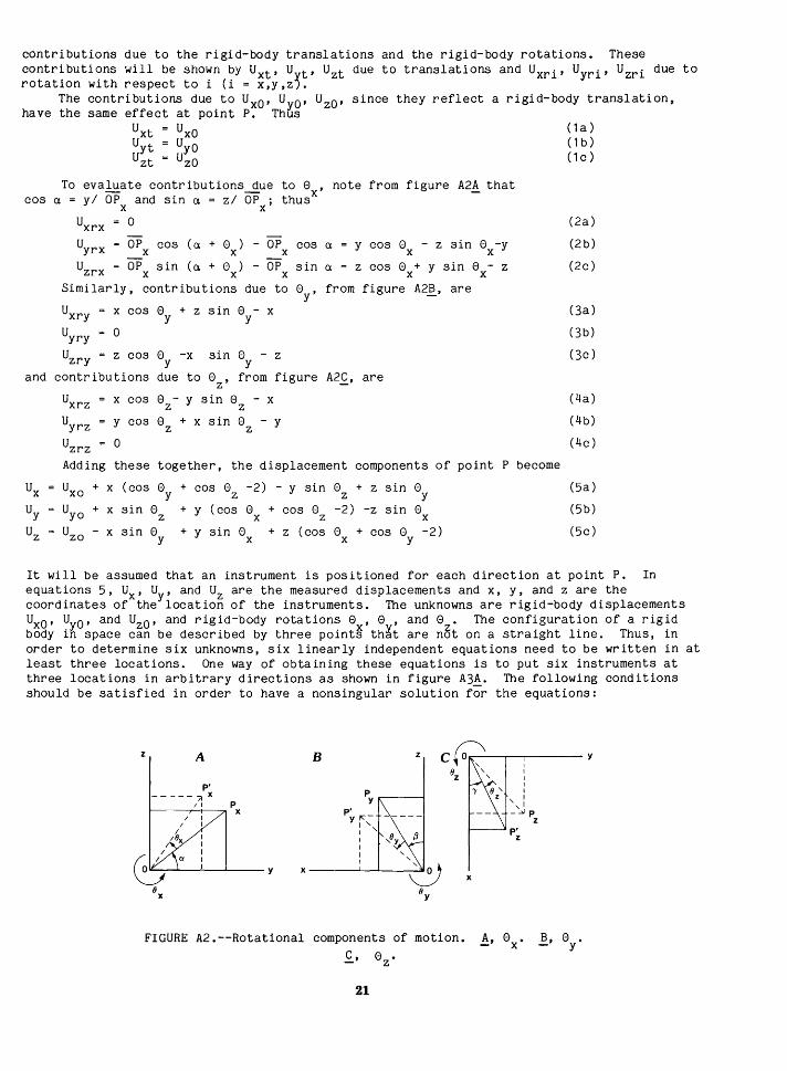
It will be assumed that an instrument is positioned for each direction at point P. In equations 5, Ux, Uy, and Uz are the measured displacements and x, y, and z are the coordinates of the location of the instruments. The unknowns are rigid-body displacements Uxo• Uyo• and Uzo• and rigid-body rotations e , e , and e . The configuration of a rigid body in space can be described by three point~ th~t are n~t on a straight line. Thus, in order to determine six unknowns, six linearly independent equations need to be written in at least three locations. One way of obtaining these equations is to put six instruments at three locations in arbitrary directions as shown in figure A3!· The following conditions should be satisfied in order to have a nonsingular solution for the equations:

z A B z c Q--r----r-1 ---- y

P' -----~~X

1-------r/---11_"71 p X

/ I

I

/IJX

~~-~~~---y IJX

P' y ~;

I ' I I I ',

x----~~--L---~

IJY

IJZ ', :

X

I I

' I ,, _->f p

z P' z

FIGURE A2.--Rotational components of motion. !• ex. .£, ez.

21

~. e . y

1. The three locations should not lie on a straight line. If they do, the rotations with respect to that line cannot be detected by the instruments.

2. Directions of instruments should not be all parallel. Otherwise, the in-plane motions perpendicular to the direction cannot be measured.

3. All directions should not intersect at one point, so that the rotations around a line through the intersection point, which is perpendicular to the plane formed by three instrumented points, can be detected.

Records from each of these instruments would provide three equations in x, y, and z directions, thus giving us 18 equations for 6 unknowns. Note that these 18 equations are not linearly independent. There are only six independent equations. Any combination of six equations written at three or more locations can be used for a solution. Another scheme of instrumentation is shown in figure A3B. In this case there are only 6 equations and measurements, all in the principal directions. They also satisfy the conditions described above; however, these equations are nonlinear and require numerical methods for solution.

Small Rotations

Nonlinear equations of motion given in equations 5a, b, and c can be linearized if the rotations e , e , and e are small. This is usually the case for many engineering problems. xThetefore, zapproximating that sine= 0 and cos 8 = 1, equations 5 become

ux uxo - y ez + z ey (6a)

Uy = Uyo + X 8z - Z 8X (6b)

u z = u - x e + y e ( 6c ) ZO y X

Now it is possible to calculate the closed-form solution. Assume, as shown in figure A3~, that ux 1 , uy 1, uz 1 were measured at point 1; uy 2 , uz 2 were measured at point 2; and uz 3 was measured at point 3. For each measurement we can write the corresponding equation from 6. Thus, we obtain six equations for six unknowns. With these equations, the rigid body translations and rotations can be calculated explicitly as given below:

u xo

u yo

u zo

e X

e y

e z

C1 y1Ux2 - y2Ux1 + (y2z1 - y1z2) · C2

y1 - y2

A

X X

FIGURE A3.--Measurements for motion in space. A, Arbitrary directions. ~' Cartesian coordinates.

22

(7a)

(7b)

( 7c)

( 8c)

where

C1

C2

C3

Uz1 (y3 - y2) + Uz2 (y1 - Y3) + Uz3 (y2 - Y1)

x1 (y2- Y3) + x2 (y3- Y1) + x3 (y1- Y2)

uz1 (x3 - x2) + uz2 ex, - x3) + uz3 (x2 - x,)

Plane Motion

Large Rotation

(9a)

(9b)

( 9c)

Sometimes the motion in one direction is zero or very small in comparison to the other two orthogonal directions because of the constraints on the structure or because of the loading and structural parameters. In this case, the motion takes place in a plane rather than in space. This simplifies the equations given above significantly.

Assume that the motion is only in the x-y plane. Making Uzo = 8 = 8 = 0 in equations 5, the equations for a plane motion can be obtained ~s y

u X

u y u

z

U + x (cos 8 - 1)- y sin 8 xO z z UyO +X sin 8z + y (cos 8z- 1)

0

( 1 Oa)

(1 Ob)

( 1 Oc)

These equations have only three unknowns, UxO' UyO' and 8 • The configuration of plane motion of a rigid body can be described by two points. Tftus, we need three measurements from at least two locations in the plane of the motion to determine the unknowns. These measurements can be in three arbitrary directions as shown in figure A4A or they can be in orthogonal directions as shown in figure A4B. The directions of instruments should satisfy the following conditions: they should not be parallel, and they should not intersect at one point.

Equations 10 can be written for each direction of each point. Any combination of three equations is sufficient to solve the unknowns; however, the equations are lengthy. A simple solution can be obtained if four measurements instead of three are made. For instance, in figure A4B, if we measure the displacements at point 1 and point 2 in both directions, using equations-10, we can write

ux1

ux2

uy,

uy2

Uxo + x, (cos 8 1) - y1 sin 8 z z

Uxo

uyo

uyo

+ x2 (cos 8 1) - y2 sin 8 z z + x1 sin 8 + y1 z

(cos 8 z 1)

+ x2 sin 8 + y 2 (cos 8 1) z z

A B y

FIGURE A4.--Measurements for motion in plane. !' Arbitrary directions. ~' Cartesian coordinates.

23

(11 a)

( 11 b)

( 11 c)

(11 d)

Note that there are only three linearly independent equations in 11. The fourth one is used for simplicity. Subtracting 11a from 11b and 11c from 11d, then eliminating (cos e - 1) in the resulting equations, one can obtain z

e z . -1 (x2- x1) (Uy2- uy1)- (y2- y1) (Ux2- Ux1) J

s1n [ 2 2

(x2- x1) + (y2- y1) ( 12a)

Once e is obtained, Uxo and Uyo can easily be calculated from equations 11a (or 11b) and 11 c (o~ 11 d). Thus

ux1 - x1 (cos ez - 1) + y1 sin ez

uy1 - x1 sin ez - y 1 (cos ez - 1)

Small Rotation

(12b)

( 12c)

When the rotation ez is small, the equations 10 can be linearized as given below:

( 13a) (13b)

We again need three equations in order to find three unknowns, UxO' UyO' and ez. Using the directions given in figure A4~, for example, one can obtain

0xo ux1 y1 <uy2 - uy1)

+ x2 - x1

( 14a)

uyo x2 uy1 - x1 uy2

X - x1 2 ( 1 4b)

uy2 - u y1 e z X - x1 2 ( 14c)

Flexible Structures

When the structure is not rigid, the instrumentation scheme given above is not sufficient to describe the motion. Flexible structures are basically structures with infinite degrees of freedom. Thus, the more instruments that are used, the better the response approximation. One practical way of instrumenting flexible structures is suggested below.

Assume that the flexible structures can be divided into imaginary small segments which are approximately rigid, as shown in figure A5A; that is, model the flexible structure as a sum of finite rigid segments. Then, instrument each segment by following the guidelines given earlier for rigid structures. In order to provide compatibility and to minimize the number of instruments, place all the instruments on the common boundaries of the segments as shown in figure A5A, so that one measurement can be used for as many segments as possible. Next, for each segment, calculate the rigid-body translations and rotations by using the equations derived earlier with respect to a coordinate system, which is located at the center of the segment and which is parallel to the global axis system. Therefore, the calculated UxO' U 0 , Uzo displacements and e , e , e rotations for each segment are the discrete values ot the overall motion at that pa~tic~lar point. Now, consider the structure as an ensemble of beam elements connecting the centers of the segments, as shown in figure A5B. Since we already know the values for the six degrees of freedom at the ends of the beams, we can calculate the values for any intermediate point through simple interpolation. A better but more expensive way of doing this would be to make a finite­element model of the structure after the measurements of each segment are obtained. Then,

24

by using the measured values as the input, the displacements and rotations can be obtained at every location.

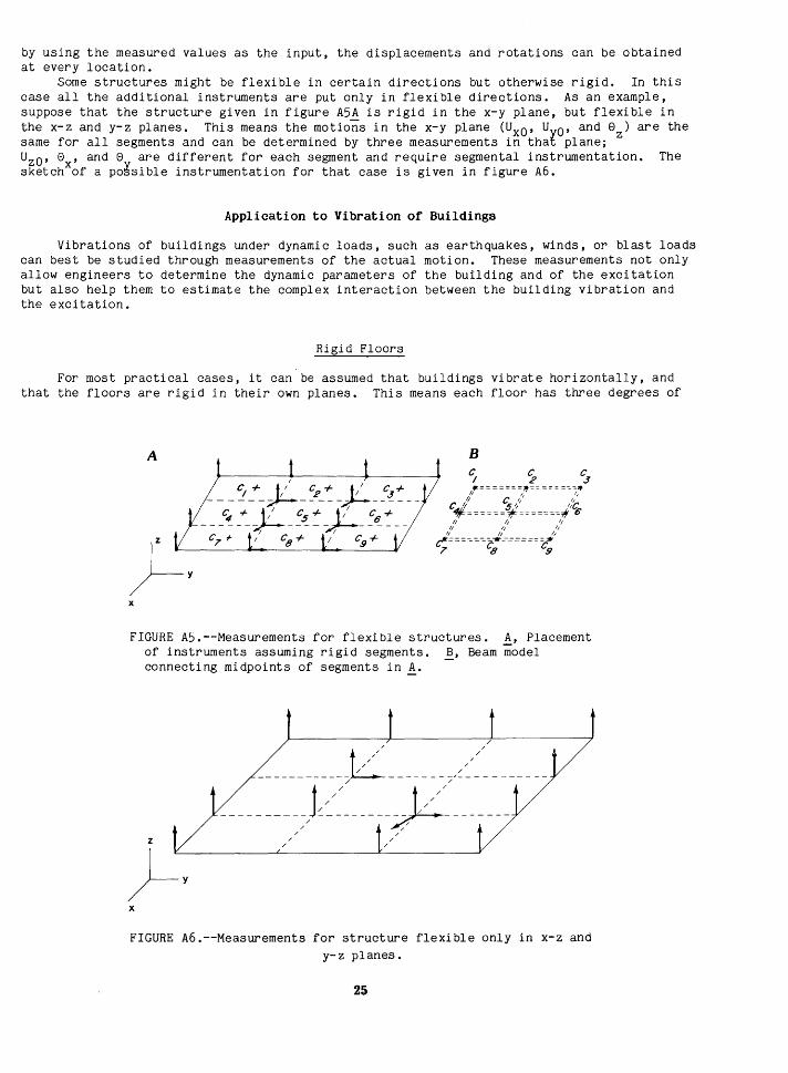
Some structures might be flexible in certain directions but otherwise rigid. In this case all the additional instruments are put only in flexible directions. As an example, suppose that the structure given in figure A5A is rigid in the x-y plane, but flexible in the x-z and y-z planes. This means the motions in the x-y plane (UxO' UYO' and 8 ) are the same for all segments and can be determined by three measurements in that plane; z U20 , e , and e are different for each segment and require segmental instrumentation. The sketchxof a po~sible instrumentation for that case is given in figure A6.

Application to Vibration of Buildings

Vibrations of buildings under dynamic loads, such as earthquakes, winds, or blast loads can best be studied through measurements of the actual motion. These measurements not only allow engineers to determine the dynamic parameters of the building and of the excitation but also help them to estimate the complex interaction between the building vibration and the excitation.

Rigid Floors

For most practical cases, it can be assumed that buildings vibrate horizontally, and that the floors are rigid in their own planes. This means each floor has three degrees of

X

FIGURE A5.--Measurements for flexible structures. A, Placement of instruments assuming rigid segments. ~' Beam model connecting midpoints of segments in A.

z

X

/ /

/

/

L/ //

---- ~~~~---_T?~--- ---JL----,~~,-~~----------~-----/ /

/ / / /

/ / / /

FIGURE A6.--Measurements for structure flexible only in x-z and y-z planes.

25

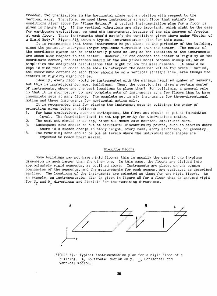
freedom; two translations in the horizontal plane and a rotation with respect to the vertical axis. Therefore, we need three instruments at each floor that satisfy the conditions given above for "Plane Motion." A typical instrumentation plan for a floor is given in figure A7A. If the vertical vibrations are also important, which might be the case for earthquake excitations, we need six instruments, because of the six degrees of freedom at each floor. These instruments should satisfy the conditions given above under "Motion of a Rigid Body." Figure A7B shows a typical instrumentation plan for this case.

It is recommended that these instruments be put close to the perimeter of the building, since the perimeter undergoes larger amplitude vibrations than the center. The center of the coordinate system can be arbitrarily placed as long as the locations of the instruments are known with respect to the center. However, if one chooses the center of rigidity as the coordinate center, the stiffness matrix of the analytical model becomes uncoupled, which simplifies the analytical calculations that might follow the measurements. It should be kept in mind that in order to be able to interpret the measured values for overall motion, the coordinate centers of each floor should be on a vertical straight line, even though the centers of rigidity might not be.

Ideally, every floor would be instrumented with the minimum required number of sensors, but this is impractical for most buildings. Thus, the question is: given a certain number of instruments, where are the best locations to place them? For buildings, a general rule is that it is much better to have complete sets of instruments at a few floors than to have incomplete sets at many floors. The complete set is six instruments for three-directional motion and three instruments for horizontal motion only.

It is recommended that for placing the instrument sets in buildings the order of priorities given below be followed: 1. For base excitations, such as earthquakes, the first set should be put at foundation

level. The foundation level is not top priority for wind-excited motion. 2. The next set should be at top, since all modes have non-zero amplitudes here. 3. Subsequent sets should be put at structural discontinuity points, such as stories where

there is a sudden change in story height, story mass, story stiffness, or geometry. 4. The remaining sets should be put at levels where the individual mode shapes are

expected to reach their maxima.

Flexible Floors

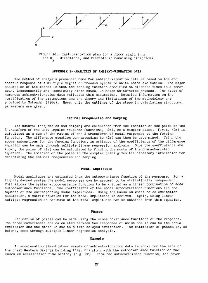
Some buildings may not have rigid floors; this is usually the case if one in-plane dimension is much larger than the other one. In this case, the floors are divided into approximately rigid segments, as outlined above. Instruments are placed on the common boundaries of the segments, and the measurements for each segment are evaluated as described earlier. The locations of the instruments are selected as those for the rigid floors. As an example, an instrumentation plan is given in figure A8 for a floor that is assumed rigid for UY and ey directions and flexible for the remaining directions.

A B

1

X

FIGURE A7.--Typical instrumentation plan for a rigid floor of a building. A, Horizontal motion only. ~, Horizontal and vertical motion.

X

FIGURE A8.--Instrumentation plan for a floor rigid in y and e directions, and flexible in remaining directions. y

APPENDIX B--ANALYSIS OF AMBIENT-VIBRATION DATA

The method of analysis presented here for ambient-vibration data is based on the sto­chastic response of a multiple-degree-of-freedom system to white-noise excitation. The major assumption of the method is that the forcing function specified at discrete times is a zero­mean, independently and identically distributed, Gaussian white-noise process. The study of numerous ambient-vibration data validates this assumption. Detailed information on the justification of the assumptions and the theory and limitations of the methodology are provided by Sotoudeh (1986). Here, only the outlines of the steps in calculating structural parameters are given.

Natura~ Frequencies and Damping

The natural frequencies and damping are calculated from the location of the poles of the Z transform of the unit impulse response functions, H(z), on a complex plane. First, H(z) is calculated as a sum of the ratios of the Z transforms of modal responses to the forcing function. The difference equation corresponding to H(z) can then be determined. Using the above assumptions for the forcing function, an estimate of the coefficients of the difference equation can be made through multiple linear regression analysis. Once the coefficients are known, the poles of H(z) can be calculated by finding the roots of the characteristic equation. The location of the poles in the complex plane gives the necessary information for determining the natural frequencies and damping.

Modal Amplitudes

Modal amplitudes are estimated from the autocovariance function of the response. For a lightly damped system the modal responses can be assumed to be statistically independent. This allows the system autocovariance function to be written as a linear combination of modal autocovariance functions. The coefficients of the modal autocovariance functions are the squares of the corresponding modal amplitudes. Using the Gaussian white noise excitation assumption, a matrix equation for the modal amplitudes is derived. Again, using linear multiple regression an estimate of the modal amplitudes can be obtained from this equation.

Phases

Estimation of phases can be made using the cross-covariance functions of the response. The cross covariances are calculated between two responses of which one is due to the actual excitation and the other is due to a time delayed excitation. The estimation of phases is, as before, done through multiple linear regression analysis.

Example

An acceleration time-history sample of ambient-vibration data is shown for the site of the Great Western Savings Building (fig. 81) along with the autocovariance function of the unsealed acceleration time history (fig. 82). From the autocovariance function, the power

27

4b

30

(/) 1-z 20 :;)

>-a: < a: 10 1-iii a: <{

~ 0

z

! 0 i= 10 <{ a: w ...J w u 20 u <{

30

40 0 100 200 300 400

TIME, IN SECONDS

FIGURE B1.--Acceleration versus time history of ambient­vibration data (units of acceleration not adjusted in accordance with recorder dynamic range, amplifier gain, and sensor sensitivity).

200

z 100 0 i= u z :;) LL

w u ~ 0 a: ~ 0 u 0 1-::> <{ 100

200oL-------------~s--------------1~o------------~15------------~2o

TIME LAG, IN SECONDS

FIGURE B2.--Autocovariance of function of unsealed acceleration time history.

28

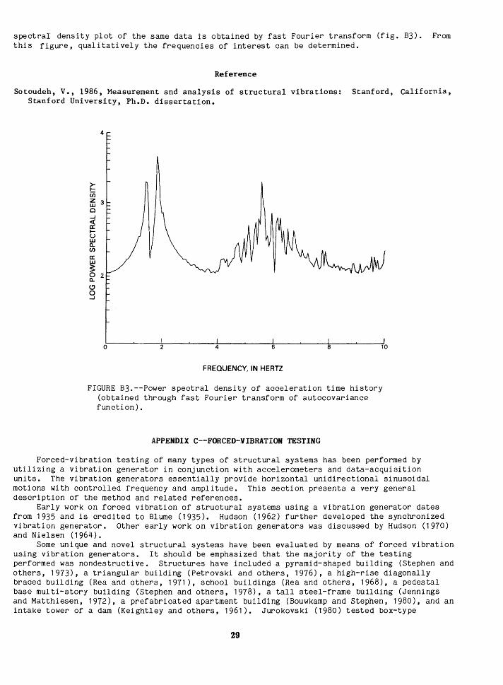
spectral density plot of the same data is obtained by fast Fourier transform (fig. B3). From this figure, qualitatively the frequencies of interest can be determined.

Reference

Sotoudeh, V., 1986, Measurement and analysis of structural vibrations: Stanford, California, Stanford University, Ph.D. dissertation.

~ (j)

4

~ 3 c ..J < a: ~ u w a.. en a: w ~ 0 2 a.. (!) 0 ..J

0 2 4 6 8 10

FREQUENCY, IN HERTZ

FIGURE B3.--Power spectral density of acceleration time history (obtained through fast Fourier transform of autocovariance function).

APPENDIX C--FORCED-VIBRATION TESTING

Forced-vibration testing of many types of structural systems has been performed by utilizing a vibration generator in conjunction with accelerometers and data-acquisition units. The vibration generators essentially provide horizontal unidirectional sinusoidal motions with controlled frequency and amplitude. This section presents a very general description of the method and related references.

Early work on forced vibration of structural systems using a vibration generator dates from 1935 and is credited to Blume (1935). Hudson (1962) further developed the synchronized vibration generator. Other early work on vibration generators was discussed by Hudson (1970) and Nielsen (1964).

Some unique and novel structural systems have been evaluated by means of forced vibration using vibration generators. It should be emphasized that the majority of the testing performed was nondestructive. Structures have included a pyramid-shaped building (Stephen and others, 1973), a triangular building (Petrovski and others, 1976), a high-rise diagonally braced building (Rea and others, 1971), school buildings (Rea and others, 1968), a pedestal base multi-story building (Stephen and others, 1978), a tall steel-frame building (Jennings and Matthiesen, 1972), a prefabricated apartment building (Bouwkamp and Stephen, 1980), and an intake tower of a dam (Keightley and others, 1961). Jurokovski (1980) tested box-type

29

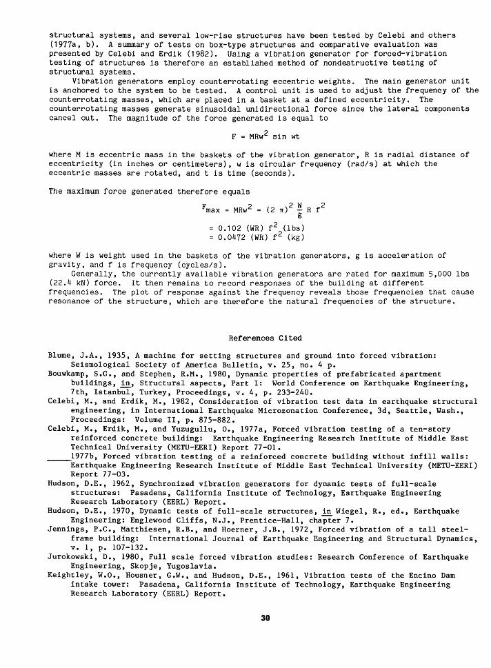
structural systems, and several low-rise structures have been tested by Celebi and others (1977a, b). A summary of tests on box-type structures and comparative evaluation was presented by Celebi and Erdik (1982). Using a vibration generator for forced-vibration testing of structures is therefore an established method of nondestructive testing of structural systems.

Vibration generators employ counterrotating eccentric weights. The main generator unit is anchored to the system to be tested. A control unit is used to adjust the frequency of the counterrotating masses, which are placed in a basket at a defined eccentricity. The counterrotating masses generate sinusoidal unidirectional force since the lateral components cancel out. The magnitude of the force generated is equal to

F = MRw2 sin wt

where M is eccentric mass in the baskets of the vibration generator, R is radial distance of eccentricity (in inches or centimeters), w is circular frequency (rad/s) at which the eccentric masses are rotated, and t is time (seconds).

The maximum force generated therefore equals

Fmax = MRw2 = (2 n) 2 ~ R f 2 g

0.102 (WR) f 2 (lbs) 0.0472 (WR) f 2 (kg)

where W is weight used in the baskets of the vibration generators, g is acceleration of gravity, and f is frequency (cycles/s).

Generally, the currently available vibration generators are rated for maximum 5,000 lbs (22.4 kN) force. It then remains to record responses of the building at different frequencies. The plot of response against the frequency reveals those frequencies that cause resonance of the structure, which are therefore the natural frequencies of the structure.

References Cited

Blume, J.A., 1935, A machine for setting structures and ground into forced vibration: Seismological Society of America Bulletin, v. 25, no. 4 p.

Bouwkamp, S.G., and Stephen, R.M., 1980, Dynamic properties of prefabricated apartment buildings, in, Structural aspects, Part I: World Conference on Earthquake Engineering, 7th, Istanbul, Turkey, Proceedings, v. 4, p. 233-240.

Celebi, M., and Erdik, M., 1982, Consideration of vibration test data in earthquake structural engineering, in International Earthquake Microzonation Conference, 3d, Seattle, Wash., Proceedings: Volume II, p. 875-882.

Celebi, M., Erdik, M., and Yuzugullu, 0., 1977a, Forced vibration testing of a ten-story reinforced concrete building: Earthquake Engineering Research Institute of Middle East Technical University (METU-EERI) Report 77-01.

_____ 1977b, Forced vibration testing of a reinforced concrete building without infill walls: Earthquake Engineering Research Institute of Middle East Technical University (METU-EERI) Report 77-03.

Hudson, D.E., 1962, Synchronized vibration generators for dynamic tests of full-scale structures: Pasadena, California Institute of Technology, Earthquake Engineering Research Laboratory (EERL) Report.

Hudson, D.E., 1970, Dynamic tests of full-scale structures, in Wiegel, R., ed., Earthquake Engineering: Englewood Cliffs, N.J., Prentice-Hall, chapter 7.

Jennings, P.C., Matthiesen, R.B., and Hoerner, J.B., 1972, Forced vibration of a tall steel­frame building: International Journal of Earthquake Engineering and Structural Dynamics, v. 1, p. 107-132.

Jurokowski, D., 1980, Full scale forced vibration studies: Research Conference of Earthquake Engineering, Skopje, Yugoslavia.

Keightley, W.O., Housner, G.W., and Hudson, D.E., 1961, Vibration tests of the Encino Dam intake tower: Pasadena, California Institute of Technology, Earthquake Engineering Research Laboratory (EERL) Report.

30

Nielsen, N. N., 1964, Dynamic response of multi-story buildings: Pasadena, California Institute of Technology, Earthquake Engineering Research Laboratory Report.

Petrovski, J., Stephen, R.M., Gartenbaum, E., and Bouwkamp, J.G., 1976, Dynamic behavior of a multistory triangular-shaped building: Berkeley, Earthquake Engineering Research Center, Report EERC 76-3, 126 p.

Rea, D., Shah, A.A., and Bouwkamp, J.G., 1971, Dynamic behavior of a high-rise diagonally braced steel building: Berkeley, Earthquake Engineering Research Center Report, EERC 71-5, 101 P•

Rea, D., Bouwkamp, J.G., and Clough, R.W., 1968, Dynamic properties of Mckinley School buildings: Berkeley, Earthquake Engineering Research Center EERC 68-4, 134 P•

Stephen, R.M., Hollings, J.P., and Bouwkamp, J.G., 1973, Dynamic behavior of a multistory pyramid shaped building, U.C. Berkeley, Earthquake Engineering Research Center Report EERC 73-17, 97 p.

Stephen, R.M., Wilson, E.L., Bouwkamp, J.G., and Button, M., 1978, Dynamic behavior of a pedestal-base multistory building: Berkeley, Earthquake Engineering Research Center, Report UCB/EERC 78-13, 145 p.

APPENDIX D--DRAFT SCHEME FOR INSTRUMENTING THE BAY BRIDGE

Introduction

An overall layout and elevation of the San Francisco-Oakland Bay Bridge is provided in figure 01. The Bay Bridge has two typical and identical suspension bridge spans (west span and east span) between San Francisco and Yerba Buena Island (fig. D2A); on the other side, between Yerba Buena Island and Oakland, there is a 1,400-ft main truss-bridge span (the cantilevered section) extending to Yerba Buena Island on the west and connected to five smaller (approximately 500 ft) truss-bridge spans on the east (fig. D2B).

In instrumenting structures of large span like the Bay Bridge, it-would ideally be of interest to develop a scheme to cover all spans. However, the return of response data from such heavy instrumentation may not necessarily justify the expenditure. This appendix provides a preliminary study; a detailed analysis and testing project is not complete, there­fore the described scheme does not follow the usual routine of analysis and testing.

Proposed Scheme

Regarding the longitudinal spacing of the instrumentation packages, it makes sense to instrument only the east suspension span and the longest truss span, located immediately west and east, respectively, of Yerba Buena Island. The central recorders could be located on Yerba Buena Island and be activated by the first of·two triggers, located at the two extremities of the instrumented sections, or by one trigger only. This would also optimize the cable layout. The only disadvantage is that the access·to data will be available only at Yerba Buena Island; however, that should not constitute a major problem.

East Suspension Span

Given the fact that for the suspension bridge (east span) the two towers, the Yerba Buena anchorage, and the center anchorage (fig. D2C) clearly have to be instrumented, one·of the remaining longitudinal locations of instruments is the center of the main span. Other locations include both third points of the main span, although if a choice is made to instrument only one third point, then it is preferable to instrument the one closer to the center anchorage as a larger response is expected there (see fig. D2C).

Each of these longitudinal locations will have a minimum of three sensors. The two towers and center anchorage will have sufficient sensors to obtain data on the-response of caissons, the deck level, and the top of the towers. Two horizontal and a vertical sensor will be required at the caisson and deck level. Additional sensors will be needed to record torsion of the double deck cross section about a longitudinal axis as well as torsion of the tower structure about a vertical axis. The main-span center locations will have sensors to monitor horizontal, vertical, and torsional motion of the deck.

31

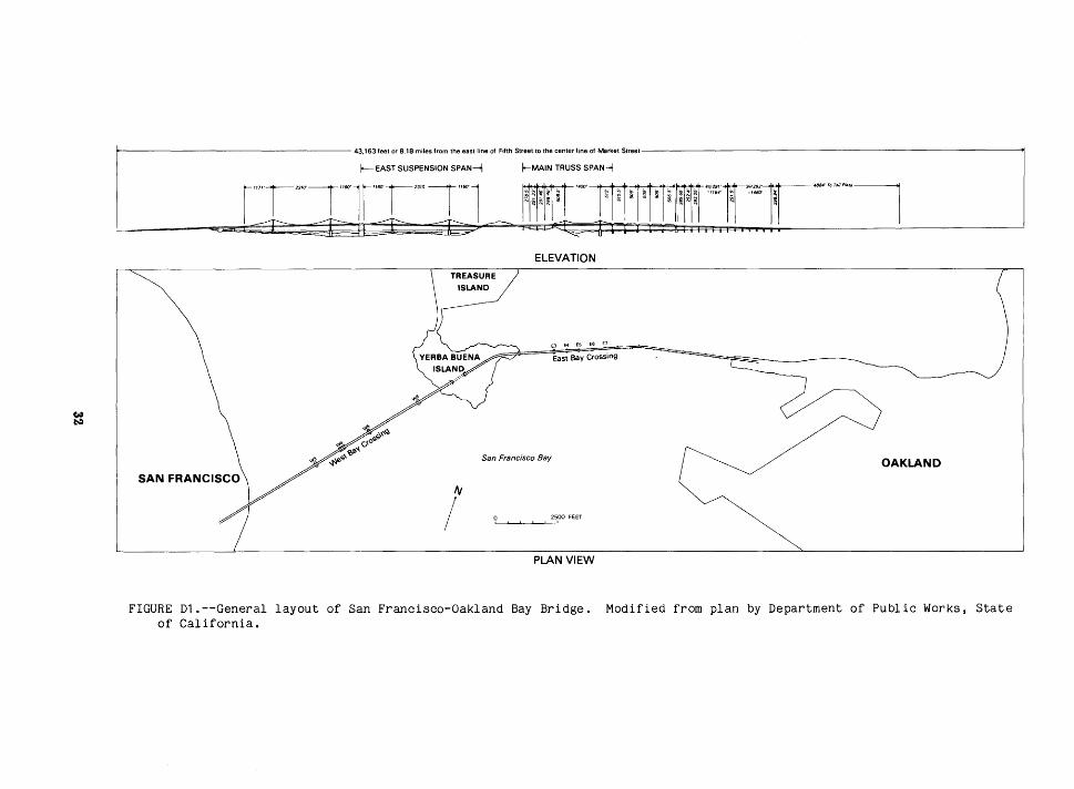
w ~

1>---------------------43,163 feet or 8.18 miles from the east line of Fofth Street to the center line of Market Street-----------------------------------ol

~EAST SUSPENSION SPAN-<\ !--MAIN TRUSS SPAN--!

rii71'123IO'III60'll"60'12310'1"60'l Err'400'~~-·@291'll3@292'--m--488.ToToi/Pim~

I I I I I I l?l;lil il I' I! I! I I IiI i 111111il "" 1'1 ~·- 111 I

4iJi ::12: ;;1?9 71=: 4?: <==:-~~ ! I I b :a I I • I I • I 6 d I I a I

TREASURE

ISLAND

ELEVATION

E3 E4 E5 E6 E7

East Bay Crossing

San Francisco Bay

/ 0 2500 FEET

PLAN VIEW

OAKLAND

FIGURE 01.--General layout of San Francisco-Oakland Bay Bridge. Modified from plan by Department of Public Works, State of California.

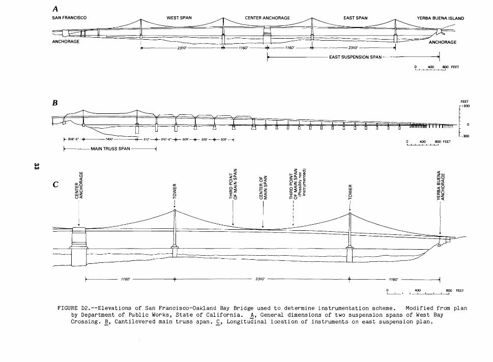
w w

A

:;; i E ::::t:::= ;;T;fNTERANCHOR======ASTSPAN:::J?z?:~ND ANCHORAGE I ==-====~ a ~ ~ANCHORAGE

-~ 2310' 1160' 1160' 2310' -----~

14------------- EAST SUSPENSION SPAN--------~

0 400 800 FEET

8 ~==== FEET +500

~ ~ ~ A ~\ l I I y ~ A A ;;::=JJ, A A A A A A A A d&i:Uillaini I I I I hi IIIII 0

io-508'-6" 1400' 512'--+-510'-6"--+- 509'-+-- 509'--+-509'---oj -300

0 400 800 FEET I I I I I I I I

it----- MAIN TRUSS SPAN -----oi

z z :0 <{w w t-~ ~~gE (!)

~(/) u.Z ~(!) <{ 0~ 0~~~ ::J<{ c ffi~ :r~ ma:: a: ffi(/) a..~,e :l a: <{0 w o<l: @~~t;; w r-::I: s a:~ t-Z s m::I: zU

:Iu. ~~ - Q.. c: a::U wz 0 :~:u._._ 0 wZ u<l: t- t-0 u~ t-0 t- >-<{

l j

I

l I I I I I ~

1160' --------------~--------------------------- 2310' 1160'

0 400 890 FEET

FIGURE 02.--Elevations of San Francisco-Oakland Bay Bridge used to determine instrumentation scheme. Modified from plan by Department of Public Works, State of California. A, General dimensions of two suspension spans of West Bay Crossing. ~, Cantilevered main truss span. £, Longitudinal location of instruments on east suspension plan.

Main Truss Span

Caisson and deck-level instrumentation of the truss span will be as in the suspension span. Abutment instruments will be located near the support on Yerba Buena Island. At midspan and third point of the truss span, horizontal and vertical sensors, as well as sensors to measure torsion of the double about the longitudinal axis motion, will be placed.

Total Instrumentation

Tables D1 and D2 show the tentative required instrumentation for suspension and truss spans, respectively. A total of approximately 41 instruments for the suspension bridge, and 30 for the cantilevered section, will be required. This means six sets of CR-1 's with 12 sensors to each set.

Additional instrumentation could be placed within some of the caissons or additional spans of the truss part of the bridge between Yerba Buena Island and toll plaza depending on the resources.

Ambient-Vibration tests could be performed before (using temporary instrumentation) or after permanent instrumentation is in place.

TABLE Dl.--Suggested instrumentation for suspension span between Yerba Buena Island and San Francisco

Location

Center anchorage At base of caisson

At deck level

Yerba Buena anchorage

Pier 5 At caisson base

At deck level At tower top

Pier 6 (same as Pier 5)

2 1 3

2 1

2 1 3 4 2

Instruments required

horizontal (1 long., vertical horizontal (1 long.,

horizontal (1 long., vertical

horizontal (1 long., vertical horizontal (1 long., horizontal (2 long., vertical

Center of main suspension span

1 transverse)

2 transverse)

1 transverse)

1 transverse)

2 transverse) 2 transverse)

1 horizontal (transverse only) 2 vertical

Third point of main suspension span

TOTAL

Additional instrumentation:

1 horizontal (transverse only) 2 vertical

Additional third point of main suspension span Midpoint of side span between Piers 4 and 5 Midpoint of side span between Pier 6 and Yerba

Buena anchorage

TOTAL

34

Total

3

3

3

3

3

6

12

3

3

41

(3) (3)

(3)

(50)

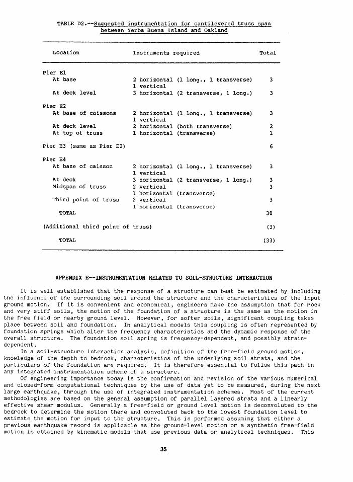
TABLE D2.--Suggested instrumentation for cantilevered truss span between Yerba Buena Island and Oakland

Location Instruments required

Pier El At base

At deck level

Pier E2 At base of caissons

At deck level At top of truss

Pier E3 (same as Pier E2)

Pier E4 At base of caisson

At deck Midspan of truss

Third point of truss

TOTAL

2 horizontal 1 vertical 3 horizontal

2 horizontal 1 vertical 2 horizontal 1 horizontal

2 horizontal 1 vertical 3 horizontal 2 vertical 1 horizontal 2 vertical 1 horizontal

(Additional third point of truss)

TOTAL

(1 long., 1 transverse)

(2 transverse, 1 long.)

(1 long., 1 transverse)

(both transverse) (transverse)

(1 long., 1 transverse)

(2 transverse, 1 long.)

(transverse)

( transverse)

Total

3

3

3

2 1

6

3

3 3

3

30

(3)

(33)

APPENDIX E--INSTRUMENTATION RELATED TO SOIL-STRUCTURE INTERACTION

It is well established that the response of a structure can best be estimated by including the influence of the surrounding soil around the structure and the characteristics of the input ground motion. If it is convenient and economical, engineers make the assumption that for rock and very stiff soils, the motion of the foundation of a structure is the same as the motion in the free field or nearby ground level. However, for softer soils, significant coupling takes place between soil and foundation. In analytical models this coupling is often represented by foundation springs which alter the frequency characteristics and the dynamic response of the overall structure. The foundation soil spring is frequency-dependent, and possibly strain­dependent.

In a soil-structure interaction analysis, definition of the free-field ground motion, knowledge of the depth to bedrock, characteristics of the underlying soil strata, and the particulars of the foundation are required. It is therefore essential to follow this path in any integrated instrumentation scheme of a structure.

Of engineering importance today is the confirmation and revision of the various numerical and closed-form computational techniques by the use of data yet to be measured, during the next large earthquake, through the use of integrated instrumentation schemes. Most of the current methodologies are based on the general assumption of parallel layered strata and a linearly effective shear modulus. Generally a free-field or ground level motion is deconvoluted to the bedrock to determine the motion there and convoluted back to the lowest foundation level to estimate the motion for input to the structure. This is performed assuming that either a previous earthquake record is applicable as the ground-level motion or a synthetic free-field motion is obtained by kinematic models that use previous data or analytical techniques. This

35

experiment will provide measurements of free-field, bedrock, and foundation motions at a single site to confirm or show inadequacies in present analyses.

The importance of developing horizontal and vertical spatial arrays to determine and confirm the change in characteristics of the media and the motion in underlying strata of a foundation has been repeatedly emphasized (Lee and others, 1978; Lysmer, 1978; and Clough, 1983). Researchers have recommended installation of arrays that will provide data on horizontal and vertical spatial variation of motion in underlying soil strata around foundations (Johnson, 1981). Instrumentation related to soil-structure interaction was a main recommendation of a recent U.S. National Workshop on Strong Motion Instrumentation (Iwan, 1981). Yet, to date, there is no such array in the United States. The only relevant arrays are the USGS Imperial Valley liquefaction array, installed to look into liquefaction problems in an area of high seismicity (Bennett and others, 1984), the USGS array near Menlo Park (Joyner and others, 1976), and some arrays in Japan (Omote and others, 1980, 1984). Ideally, the following studies will be required to answer some of the questions that have been raised:

1. Study by instrumentation with boreholes the effect on ground level motion of varying depths of different underlying soil layers under near-source and far-source conditions. Sites should be found where there are distinct layers of the following foundation soils:

granular or alluvial silty clay soft clay hard soil (stiff soil) rock

The sites should be near a fault with high probability of occurrence of earthquakes. Preferably, there should be a structure within 5-10 km of the fault (near-source studies) and another within 50 km of the fault.

2. Study by subsurface instrumentation with boreholes the horizontal and vertical spatial variation of seismic waves for varying underlying soil strata. This scheme should include (1) instrumentation on a vertical array directly under a foundation; (2) instrumentation around the perimeter of a foundation to look into separation of the foundation from soil; and (3) instrumentation on a horizontal array near a building to capture the horizontal variation of free-field motion. Preferably the last one can be done in two orthogonal directions to study the idealization of three-dimensional motion into two-dimensional motion.

3. Study by instrumentation the effect of different types of foundation. Possible foundation types to be looked into include deeply embedded mat foundation, mat foundation, mat or footing foundations with piles, and footings and spread footings.

4. Study dynamic properties of soil layers within the above instrumentation schemes.

5. Study by instrumentation the influence of strain softening of soil by liquefaction or weakening of sensitive clay on structural response. One area where this phenomenon has occurred is Anchorage, Alaska.

6. Development of specific instrumentation if necessary and instrumentation schemes to detect the motion of layered strata, as well as separation between foundation and soil.

A general schematic of the "integrated" array systems is shown in figures E1 and E2.

References Cited

Bennett, M.J., McLaughlin, P.V., Sarmiento, J.S., and Youd, T.L., 1984, Geotechnical investigation of liquefaction sites, Imperial Valley, California: U.S. Geological Survey Open-File Report 84-252.

Clough, G.W., editor, 1983, A report of the Workshop on Research Needs in Experimental Soil Engineering: Blacksburg, Virginia Polytechnic Institute.

Iwan, W.D., editor, 1981, U.S. strong-motion earthquake instrumentation:, U.S. National Workshop on Strong-Motion Earthquake Instrumentation, April 1981, Santa Barbara, California, Proceedings, California Institute of Technology, 69 p.

36

Johnson, J.J., 1981, Soil structure interaction: The status of current analysis methods and research: Washington, D.C., Nuclear Regulatory Commission, Report NUREG-CR-1780.

Joyner, W.B., Warrick, R.E., and Oliver, A.A., 1976, Analysis of seismograms from a downhole array in sediments near San Francisco Bay: Seismological Society of America Bulletin, v. 66, no. 3, p. 957-958.

Lee, K.L., and others, 1978, Workshop on Research needs and priorities for Geotechnical Earthquake Engineering Applications: Arlington, University of Texas.

Lysmer, J., 1978, Analytical procedures in soil dynamics: Geotechnical Engineering Specialty Conference on Earthquake Engineering and Soil Dynamics, Pasadena, Calif., Report PB-298455.

Omote, S., Ohmatsuzawa, K., and Ohta, T., 1980, Recently developed strong motion earthquake instruments array in Japan, in Geoscience aspects, Part II: World Conference on Earthquake Engineering, 7th, Istanbul, Turkey Proceedings, v. 2, p. 41-48.

Omote, S., and others, 1984, Observation of earthquake strong-motion with deep boreholes--An introductory note for Iwaki and Tomioka observation station in Japan, in Ground motion and seismicity: World Conference on Earthquake Engineering, 8th, San Francisco, Calif., Proceedings. v. II, p. 247-254.

~~~~~~~~~~0-is_~_n_c_e_t_o_e_P_~_e_n_~_r~~~~~~~~~~ BUILDINGINSTRUMEN~TION Instrumentation nth floor

A

Strong-motion

around perimeter r-r..-../-... (translation, torsion) of foundation

Horizontal free- \ field arrays

Mid-floors (translation, torsion)

Foundation

dense arrays )

_~5!._0 .2.0_50~------~~ ~-cWnf.c

0 0 0 I

0 I

(translation, torsion, rocking) Ground level

1::<: /~~ Source of

earthquake

* B

Strata thickness and sensors for vertical

spatial variation

Horizontal array

Horizontal array ,,_,-_ __...,......_..._ _____ \ 0 0 0 0

I

0 I

I 0

~ Planof ~ foundation

Height

FIGURE E1 .--Qualitative description of an integrated instrumentation scheme. A' Vertical cross section. ~' Plan view of horizontal free-field array.

37

Free field •

Strata thickness ---- ----- -----and sensors

for vertical spatial variation __ _

0

• 0

Building

with

specific

instrumentation

• • 0 • • 0

EXPLANATION

• 0

Vertical accelerometer

Three-dimensional accelerometer

Pressure gauge

-- Horizontal accelerometer

Ground level ,0-- ~

~

--45 --·----~4 Height

• h3

-------f • h2

-------f • •

y // ""' ---"77" "'-"' / ~ ""' "" Bedrock

FIGURE E2.--Qualitative description of instrumentation around boundary and below foundation of a building.

38

GPO 785-048/48040