Embed Size (px)
Citation preview
Integrated Thermal and Energy Management of
Plug-in Hybrid Electric Vehicles
By
Mojtaba Shams-Zahraei (M.Sc.)
Submitted in fulfilment of the requirements for the degree of
Doctor of Philosophy
Deakin University
August 2012


To my beautiful wife, Tina

I
ACKNOWLEDGMENTS
First and foremost, I would like to acknowledge respectfully, the help and
support I have received from my supervisor, Assoc. Prof. Abbas Kouzani, who
has been an enduring mentor, a great teacher, and a patient friend at all stages of
my PhD candidature. I would also like to thank my co-supervisor Assoc. Prof.
Hieu Trinh and of course all my friends and colleagues at Deakin University. The
help and support I received from the lovely staff of School of Engineering and
Higher Degree by Research is highly appreciated.
I would like express my gratitude to Prof. Bernard Baker for his support both
financially and academically during my research stay at Institute of Automotive
Technology Dresden/ Germany (IAD). I am grateful to all of my friends and
colleagues at IAD for their help, discussion, and all the good times we shared.
Especially I thank Steffen Kutter who facilitates the great research stay in Germany.
I would also like to thank my dear family, as their moral support has never
ceased in my life and is always keeping me motivated and strong.

II
ABSTRACT
Plug-in hybrid electric vehicles (PHEVs) benefit from the features of both
conventional hybrid electric vehicles (HEVs) and electric vehicles (EVs) by
having a large battery which can be recharged when plugged into an electric
power source. PHEVs are creating much interests due to their significant potential
to improve fuel efficiency and reduce emissions particularly for daily commuters
with short daily trips. PHEVs would be the next generation of vehicles in the
market before full electrification of vehicles becomes mature. The aim of this
research is to find the most efficient energy management strategy (EMS) to
control the energy flow in the powertrain components of PHEVs. The simulations
are conducted on a serial drivetrain model; however, the presented approach for
EMS of PHEV in this thesis is equally applicable for other available hybrid
architectures. The thesis also gives a review of control approaches that are
exclusively applicable for the EMS of PHEVs.
The implementation of globally optimal energy management strategies is only
feasible when an accurate prediction of driving scenario is available. There are
many noise factors which affect both the drivetrain power demand and the vehicle
performance even in identical drive-cycles. In this research, the effect of each
noise factor is investigated by introducing the concept of power-cycle instead of
III
drive-cycle for a journey. A practical solution for developing a power-cycle
library is introduced to improve the accuracy of power-cycle prediction.
PHEVs employ a rechargeable battery as an energy source alongside a fuel
source. Consequently, in PHEVs the engine temperature declines due to the
reduced engine load as well as the extended engine off period. It is proven that the
engine efficiency and emissions depend on the engine temperature. Moreover,
temperature, as one of the noise factors, has direct influence on the vehicle air-
conditioner and the cabin heater loads. Particularly, while the engine is cold, the
power demand of the cabin heater needs to be provided by the battery instead of
the waste heat of the engine coolant. Existing studies on EMS of PHEVs mostly
focus on the improvement of fuel efficiency based on the hot engine
characteristics neglecting the effect of temperature on the engine performance and
the vehicle power demand. This thesis presents two new EMSs which consider the
temperature noise factor to maximise the performance and the efficiency of
PHEVs for a predefined journey. First, a rule-based approach to find the best
charge depleting regime of battery is introduced. The rule-based approach is a
sub-optimal solution for the control problem but is easily implementable, as it
requires limited computation effort. The second approach incorporates an engine
thermal management method, which formulates the globally optimal battery
charge depleting trajectories based on the Bellman’s principle of optimality. A
dynamic programming-based algorithm is developed and applied to enforce the
charge depleting boundaries while optimizing a fuel consumption cost function by
controlling the engine power as an input variable. The optimal control problem
formulates the cost function based on two major state variables: battery charge

IV
and internal temperature. The algorithm also considers a minimum duration for
which the engine is allowed to switch from on to off modes preventing the
concerns associated with the engine transient operation. It is demonstrated that the
temperature and the cabin heater/air-conditioner power demand, even in an
identical drive-cycle, can significantly influence the optimal solution for the EMS,
and accordingly the fuel efficiency and the emissions of PHEVs.

V
List of Publications
M. Shams-Zahraei, A. Z. Kouzani, S. Kutter, and B. Bäker, "Integrated thermal
and energy management of Plug-in hybrid electric vehicles," Journal of Power
Sources, vol. 216, pp. 237-248, will be published in 15 October 2012.
M. Shams-Zahraei, A. Z. Kouzani, and B. Ganji, “Effect of noise factors in
energy management of series plug-in hybrid electric vehicles," International
Review of Electrical Engineering, vol. 6, pp. 1715-1726, 2011.
M. Shams-Zahraei and A. Z. Kouzani, “Effect of temperature noise factor in
energy management of series plug-in hybrid electric vehicles” presented at Energy
Efficient Vehicle Technology, Dresden, Germany, 2011.
M. Shams-Zahraei and A. Z. Kouzani, "Power-cycle-library-based control
strategy for plug-in hybrid electric vehicles," presented at the IEEE Vehicle Power
and Propulsion Conference Lille, France, 2010.
M. Shams-Zahraei and A. Kouzani, "A study on plug-in hybrid electric
vehicles," presented at the TENCON IEEE Conference, Singapore, 2009.
B. Ganji, A. Kouzani, Kh.S. Yang, and M. Shams-Zahraei, "Adaptive cruise
control of hybrid electric vehicle based on sliding mode control" under review.

VI
Table of content
Acknowledgement .......................................................................................... I
Abstract ........................................................................................................ II
List of publication ......................................................................................... V
Table of content .......................................................................................... VI
List of figures ................................................................................................ X
List of tables ............................................................................................... XII
Chapter 1. Introduction .................................................................................1
1.1 Motivation ................................................................................................1
1.2 Hybrid electric vehicles ............................................................................3
1.3 Plug-in hybrid Electric Vehicles ..............................................................5
1.3.1 Extended-Range Electric Vehicle ..................................................................... 7
1.3.2 Definition of operating modes for PHEVs and EREV ....................................... 7
1.3.3 HEV and PHEV powertrain architecture ........................................................... 8
1.3.4 Drivetrain compatibility for PHEV applications .............................................. 12
1.4 Pathway for better fuel Economy .......................................................... 17
1.4.1 Efficiency of PHEV components .................................................................... 19
1.4.2 Auxiliary loads .............................................................................................. 24
1.4.3 Energy management strategy .......................................................................... 25
1.5 Research aim, objectives and Contributions ......................................... 26
1.6 Outline of the thesis ................................................................................ 28
Chapter 2. Review on energy management strategies for HEVs and
PHEVs ........................................................................................................... 30
VII
2.1 Introduction............................................................................................ 30
2.2 Power, energy, and charge management strategy ................................. 31
2.2.1 PHEV operation modes .................................................................................. 32
2.3 classification of Energy management strategies .................................... 33
2.3.1 Rule-based controllers .................................................................................... 34
2.3.2 Optimization based controllers ....................................................................... 35
2.4 EMSs exclusively Developed for PHEVs ............................................... 39
2.5 conclusion ............................................................................................... 42
Chapter 3. Vehicle modelling ...................................................................... 43
3.1 Introduction............................................................................................ 43
3.2 Longitudinal dynamics of vehicles ......................................................... 44
3.3 Methods of modelling ............................................................................. 45
3.3.1 The average operating point approach ............................................................ 45
3.3.2 The quasi-static approach ............................................................................... 46
3.3.3 Dynamic approach ......................................................................................... 47
3.4 Forward and backward modelling approaches ..................................... 47
3.4.1 Backward approach ........................................................................................ 47
3.4.2 Forward approach .......................................................................................... 48
3.5 Simulation tools ...................................................................................... 49
3.6 Modelling approach used in this work................................................... 50
3.6.1 Drivetrain architecture and sizing of the sub-models ....................................... 51
3.6.2 Internal combustion engine ............................................................................ 54
3.6.3 Battery model ................................................................................................ 62
3.6.4 Electric motor/generator ................................................................................. 68
3.6.5 Transmission and final drive .......................................................................... 69
VIII
3.6.6 Wheel and axel .............................................................................................. 69
3.6.7 Vehicle model ................................................................................................ 70
3.7 Conclusion .............................................................................................. 72
Chapter 4. Noise factors and power cycle prediction ................................. 73
4.1 Introduction............................................................................................ 73
4.2 Power-cycle and Noise Factors .............................................................. 75
4.2.1 Power-cycle library ........................................................................................ 76
4.2.2 Noise factors .................................................................................................. 78
4.3 conclusion ............................................................................................... 87
Chapter 5. Energy management of PHEVs: A Rule based approach ....... 89
5.1 Introduction............................................................................................ 89
5.2 AER-CS energy management ................................................................ 90
5.2.1 Confined optimal operation line ..................................................................... 92
5.2.2 Driving scenario............................................................................................. 93
5.3 Proposed Rule based blended mode EMS ............................................. 94
5.3.1 Step 1: Hot engine efficiency cycle, CD1 strategy ........................................... 96
5.3.2 Step 2: Engine warmth conservation, CD2 strategy ....................................... 101
5.3.3 Step 3: Engine cold start investigation, CD3 strategy .................................... 102
5.3.4 EMS for the cold weather ............................................................................. 105
5.4 Results .................................................................................................. 106
5.5 Conclusion ............................................................................................ 111
Chapter 6. Optimal integrated thermal and energy management of PHEVs
......................................................................................................................... 113
6.1 Introduction.......................................................................................... 113
6.2 Optimal control and dynamic programming ...................................... 114
IX
6.2.1 Mathematical modelling for dynamic approach ............................................. 115
6.2.2 The performance measure or the cost function .............................................. 116
6.2.3 The principle of optimality ........................................................................... 116
6.3 EMS of PHEVs and dynamic Programming ....................................... 117
6.3.1 Vehicle model .............................................................................................. 118
6.3.2 Initialization of DP approach ........................................................................ 123
6.3.3 Cost-to-go matrix ......................................................................................... 124
6.3.4 Forward DP instead of backward DP ............................................................ 132
6.4 Simulation Results ................................................................................ 132
6.4.1 Driving scenario........................................................................................... 133
6.5 Real-time Implementation ................................................................... 143
6.6 Conclusion ............................................................................................ 145
Chapter 7. Conclusion and future work ................................................... 147
7.1 Conclusion ............................................................................................ 147
7.2 Future work .......................................................................................... 151
Bibliography .............................................................................................. 153
Appendix A. Nomenclature ....................................................................... 165
X
List of figures
Figure 1.1.Cumulative distribution of daily driving distances in Australian cities ......................... 6
Figure 1.2. (A) Series drivetrain. (B) Parallel drivetrain. (C) Series-parallel drivetrain ............... 9
Figure 1.3. BSFC and efficiency map of two typical engines ....................................................... 21
Figure 1.4. Toyota Prius Gen.1 traction motor efficiency map .................................................... 22
Figure 1.5. Equivalent circuit for a battery ................................................................................ 23
Figure 2.1. PHEV operation modes ........................................................................................... 33
Figure 2.2. Control problem formulation tree for the EMS of PHEVs ......................................... 34
Figure 3.1. Vehicle loads and environmental parameters which affect
the longitudinal dynamics of a vehicle. ...................................................................................... 45
Figure 3.2. Schematic of the serial EREV components with a
combined electric/engine-coolant cabin heater .......................................................................... 53
Figure 3.3. Block diagram of the series HEV architecture .......................................................... 54
Figure 3.4. Engine efficiency map .............................................................................................. 55
Figure 3.5. Schematic illustration of the engine thermal model................................................... 57
Figure 3.6. Battery characteristics (25 series, 10 parallel battery cells)...................................... 64
Figure 3.7. Schematic of the battery thermal model .................................................................... 66
Figure 3.8. Electric motor efficiency map .................................................................................. 68
Figure 4.1. Required inputs for developing the power-cycle library ............................................ 77
Figure 5.1. Schematic representation of power follower rules .................................................... 90
Figure 5.2. Confined optimal operation line ............................................................................... 93
Figure 5.3. Three-step rule-based blended mode EMS................................................................ 96
Figure 5.4. Schematic illustration of Step 1 ................................................................................ 99
Figure 5.5. Flowchart of the process to find the position of the efficiency line in CD1............... 100
Figure 5.6. (a) Defined mirrored drive-cycle and elevation. (b) Power and equivalent efficiency
cycle and efficiency line in CD1. (c) Engine coolant temperature and cold-factor for CD2. (d)
Power and equivalent efficiency cycle modified by cold-factor and efficiency line in CD2. (e)
XI
Power and equivalent efficiency cycle and efficiency line in CD3. (f) Coolant temperature in CD1,
CD2, and CD3 ........................................................................................................................ 104
Figure 5.7. Engine operation points in the efficiency map. (a) AER/CS strategy. (b) CD3 strategy
............................................................................................................................................... 107
Figure 5.8. Battery SOC history, current, and temperature in both the AER-CS and the CD3.... 110
Figure 6.1. Graphical representation of cost-to-go matrix ........................................................ 127
Figure 6.2. Schematic calculation of cost-to-go for each node .................................................. 130
Figure 6.3. Flowchart of the developed dynamic programming code ........................................ 131
Figure 6.4. Simulation results for a warm day with 1.5 kW constant AC power demand and cool-
down period at t=3500 (A) drive-cycle and elevation profile, (B) power-cycle, (C) engine power
trajectory of AER-CS EMS, (D) engine power trajectory of blended mode EMS by DP without
cold-factor, (E) engine power trajectory of blended mode EMS by DP with cold-factor, (F) battery
SOC trajectories, (G) engine coolant temperature trajectories, and (H) fuel consumption
trajectories .............................................................................................................................. 137
Figure 6.5. Simulation results for a chilly day with 3 kW constant heater power demand without a
cool-down period (A) drive-cycle and elevation profile, (B) engine power of AER-CS EMS of a
vehicle with all electric heater (C) engine power of AER-CS EMS, heater power demand is
supplied by engine waste heat if ˚C (D) engine power of CD EMS with cold-factor and
heater power demand, heater power demand is supplied by engine waste heat if ˚C (F)
coolant temperature trajectories (G) fuel consumption trajectories .......................................... 141
Figure 6.6. A superimposed selected section of Figure 6.4(B) and (D) ...................................... 143
Figure 6.7. (A) Comparison of the coolant temperature trajectories in ADVISOR and DP with
cold-factor simulations for (A) Warm day (B) Chilly day .......................................................... 145

XII
List of tables
Table 3-1 Powertrain model specifications ................................................................................ 53
Table 3-2. Definition of parameters used for engine thermal model ............................................ 61
Table 5-1. Performance comparison of the AER-CS and the rule-based blended strategies ....... 109
Table 6-1. DP and ADVISOR simulation results for warm day ................................................. 138
Table 6-2. DP and ADVISOR simulation results for chilly day ................................................. 142
1
CHAPTER 1
INTRODUCTION
1.1 MOTIVATION
Living in the era of increasing environmental sensibility and rise in fuel price
makes it necessary to develop new vehicles that are more fuel efficient and
environmental friendly. The oil price has risen almost fourfold since 10 years ago
and is likely to continue to increase in the future because of shrinking oil supplies
and surge in demand. Increasing concerns about environmental issues, such as
global warming and greenhouse gas emissions, boost the feasibility of new
technologies of green vehicles. Implementation of fuel-economy regulations and
Chapter 1
2
ever-tightening emission standards are major technology challenges that all
automotive manufacturers currently face.
Electrification of vehicle drivetrains has been a major breakthrough to realise
the reduction of fuel consumption and emission ambitions without sacrificing
performance. An electric vehicle (EV) was once considered as a promising
alternative for a conventional vehicle due to good overall efficiency, low audible
noise, and zero on-board emissions. Nevertheless, technological and financial
barriers regarding electrical storage devices such as batteries and super-capacitors
delayed fully commercialization of electric vehicles. Still, available EVs in the
market suffer from high cost and rang-anxiety issues. Hybrid electric vehicles as
the second option (HEVs) have been available in the market since 1997, and their
market share has improved since then. Plug-in hybrid electric vehicles (PHEVs)
benefit from the features of both conventional HEVs and EVs. PHEVs have a
large battery which can be recharged when plugged into an electric power source
alongside an engine to replenish the battery for long journeys. The features of
PHEVs are appealing for daily commuters since the larger battery could supply
energy demand of short journeys and the combustion engine could realise the
range extension. PHEVs could be a short-term solution before the technological
barriers for full electrification of vehicles are overcome.
The highest level of powertrain control in HEVs or PHEVs is an energy
management strategy (EMS) that interprets the driver power demand for
drivetrain components. The EMS decides how to distribute the vehicle power
demand between the electric power path and the conventional mechanical power
path efficiently. The extra available energy source, the battery charge of PHEVs,
Chapter 1
3
adds an extra dimension to the complexity of the EMS control problem compared
to HEVs in which the engine is the sole source of energy. Therefore, to achieve
full benefit out of having an extra energy source on-board, a charge management
strategy should be incorporated into the EMS. The extra energy source also results
in a decline in the engine temperature due to reduced engine load as well as
extended engine off periods. It is well known that engine efficiency and emissions
depend on the engine temperature. Moreover, temperature has direct influence on
the vehicle air-conditioner and the cabin heater loads. Particularly, while the
engine is cold, the power demand of the cabin heater needs to be provided by the
battery instead of the waste heat of the engine coolant. This thesis addresses the
sensitivity of PHEVs’ drivetrain performance with regard to the temperature
noise-factor. This research proposes methodologies based on a rule-based as well
as an optimal control theory method to derive an optimal charge depleting
trajectory for the PHEV battery. The significance of temperature on the optimal
EMS of PHEVs is also demonstrated. The resulted charge management coincides
with the optimal thermal management of the engine for minimum fuel
consumption, while maximizing the use of the engine waste heat for the cabin
warming in place of the battery electricity in cold weather.
1.2 HYBRID ELECTRIC VEHICLES
Hybrid vehicles benefit from an efficient combination of at least two power
sources to propel the vehicle. Generally, one or more electric motors alongside an
Internal Combustion Engine (ICE) or a fuel cell, as a primary energy source,
operates the propulsion system of HEVs. A battery or a super-capacitor as a
Chapter 1
4
bidirectional energy source provides power to the drivetrain, also recuperates part
of the braking energy dissipated in conventional ICE vehicles. Usually the term
HEV is used for a vehicle combining an engine with an electric motor. Hybrid-
Inertia, Hybrid-Hydraulic, and fuel cell propulsion systems are also considered as
members of the HEVs family.
The main advantages of the HEV drivetrain are as follows:
ICE downsizing: Since the peak power demand could be provided by a
combination of the ICE and the battery, the ICE could be sized for average
power demand of the vehicle. This reduces the weight and improves the
efficiency of the ICE when operating at the same load of a larger engine.
Regenerative braking: The on-board battery or super-capacitor of HEV can
be recharged while the electric motor operates in the generator mode
providing braking force instead of friction brake.
Engine on/off functionality: The engine can be turned off when the vehicle
is at standstill or the vehicle power demand is low. This prevents
unnecessary engine idling or its operation at low power which is generally
inefficient.
Control flexibility: The additional degree of freedom to provide the
vehicle power demand from either of the power sources gives the
flexibility to operate the powertrain components in a more efficient
manner.
Chapter 1
5
A more extensive introduction to HEVs and modern vehicle propulsion
systems can be found in the literature [1-5].
1.3 PLUG-IN HYBRID ELECTRIC VEHICLES
Plug-in hybrid electric vehicles (PHEVs) benefit from the features of both
conventional HEVs and electric vehicles (EVs) by having a large battery which
can be recharged when plugged into an electric power source. A PHEV is a viable
solution to replace some part of the energy used in vehicular transportation with
electricity, before full electrification of vehicles becomes mature [6]. Moreover,
PHEVs can eliminate concerns about EVs’ recharging time and range anxiety.
PHEVs have considerable influence on the shift from fossil fuels to electric
energy sources for significant part of daily commutes. Hence, according to an
investigation conducted by Toyota, the accumulative daily travel of around 75%,
80%, and 95% of vehicles in North America, Europe, and Japan are lower than 60
km, respectively [7]. The cumulative daily travel in Australian cities is depicted in
Figure 1.1.
Chapter 1
6
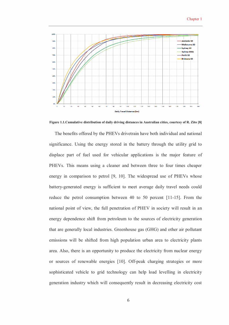
Figure 1.1.Cumulative distribution of daily driving distances in Australian cities, courtesy of R. Zito [8]
The benefits offered by the PHEVs drivetrain have both individual and national
significance. Using the energy stored in the battery through the utility grid to
displace part of fuel used for vehicular applications is the major feature of
PHEVs. This means using a cleaner and between three to four times cheaper
energy in comparison to petrol [9, 10]. The widespread use of PHEVs whose
battery-generated energy is sufficient to meet average daily travel needs could
reduce the petrol consumption between 40 to 50 percent [11-15]. From the
national point of view, the full penetration of PHEV in society will result in an
energy dependence shift from petroleum to the sources of electricity generation
that are generally local industries. Greenhouse gas (GHG) and other air pollutant
emissions will be shifted from high population urban area to electricity plants
area. Also, there is an opportunity to produce the electricity from nuclear energy
or sources of renewable energies [10]. Off-peak charging strategies or more
sophisticated vehicle to grid technology can help load levelling in electricity
generation industry which will consequently result in decreasing electricity cost

Chapter 1
7
because of reduction in power plant start-up, operation, and maintenance costs
[12]. However, the battery charging strategies significantly affect the electricity
consumption from the power generation point of view [16].
1.3.1 Extended-Range Electric Vehicle
Extended-range electric vehicles (EREVs) are PHEVs that can operate on a
pure electric vehicle (EV) mode. Both the battery and the tractive motor of
PHEVs are capable of providing maximum tractive and auxiliary power demand
for the powertrain. The maximum range that can be covered on the EV mode for a
standard power-cycle is called all electric range (AER) for the specific cycle. The
market of EREVs is focused on daily commuters who prefer the benefits of
driving on the EV mode for daily routine travels while enjoying the driving
without the range-anxiety for longer journeys.
1.3.2 Definition of operating modes for PHEVs and EREV
Charge Depleting and EV mode
Charge depleting (CD) refers to a PHEV operation mode in which the
vehicle drains energy from the charged battery. However, sometimes
because of the drivetrain restrictions, the engine operation is inevitable.
The EV mode is a special case of the charge depleting. During the EV
mode, the engine is turned off and the vehicle only relies on the battery
energy to cover both the tractive and ancillary loads.
Charge sustaining (CS) mode

Chapter 1
8
Similar to HEVs, the battery charge is sustained around a predefined
range. Generally, the CS mode happens when the battery is completely
depleted to the minimum applicable threshold for the battery state of
charge (SOC). That is, the PHEV operates like a conventional HEV when
the SOC reaches the minimum applicable SOC defined for the battery.
Blended mode
In the blended mode, both the engine and the battery provide the
required power demand for the vehicle. Generally, the control strategy of
PHEV selects the ratio of the engine to the battery power in a more
efficient fashion. That is, in comparison the simple CD, a blended mode
possesses a more intelligent charge management strategy.
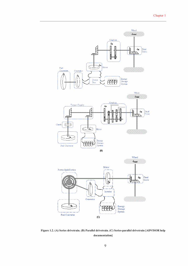
1.3.3 HEV and PHEV powertrain architecture
The combinations of connections between components of the propulsion
system define the architecture of HEVs. Conventionally, HEVs are categorized
into three basic drivetrain architectures: series, parallel, and series-parallel. A
schematic representation of these three basic architectures is given in Figure 1.2.
Detailed descriptions of the characteristics of each drivetrain can be found in the
literature [1-4]. This introduction focuses on the characteristics that distinguish
between these powertrain architectures for PHEV applications.
Chapter 1
9
Figure 1.2. (A) Series drivetrain. (B) Parallel drivetrain. (C) Series-parallel drivetrain [ADVISOR help
documentation]

Chapter 1
10
The series configuration is commonly recognized as an electric vehicle that has
an engine and a generator to recharge the battery so it is easier to upgrade it to a
PHEV. The series architecture is a common drivetrain for diesel-electric
locomotives and ships. The series architecture drivetrain has a sized electric motor
to coupe the designed vehicle maximum traction power. The increase in power
capacity of the battery enables the AER and the zero emission operation of the
series architecture. Since there is no mechanical coupling between the wheels and
the engine in this architecture, the engine can operate independently around its
most efficient torque-speed region. However, the well-known drawback of the
series drivetrain is the conversion of the engine mechanical power to electrical
and then back to mechanical form in the electric motor. This efficiency chain
reduces the overall efficiency of the drivetrain. For example, GM Volt is a 64 km
EREV with a base platform of series drivetrain. Volt benefits from a mode
changing architecture by employing a planetary-gear-set and two brakes. The
mechanism enables the vehicle to shift from the series to the series-parallel
architecture to solve the above-mentioned drawback. In this mode, the engine
could mechanically transfer power to the final-drive in higher vehicle speeds and
power demands. Also, it has two different EV modes in which the EV mode is
shifted from one electric motor drive to two electric motor drives in order to
reduce the losses associated with high speed operation of the electric motors,
particularly during cruise operation [17]
In parallel drivetrain, both the engine and the electric motor can propel the
wheels directly (see Figure 1.2 (B)). Properly sized electric motor and battery are
necessary to upgrade a parallel drivetrain to an EREV. In the pre-transmission

Chapter 1
11
parallel architecture similar to that of Honda Insight, Civic, and Accord HEVs, a
small electric motor is located between the engine and the transmission replacing
the flywheel [18]. It is also possible for a parallel HEV to use its engine to drive
one of the vehicle axles, while its electric motor drives the other axle. Daimler
Chrysler PHEV Sprinter has this powertrain configuration. A direct mechanical
connection between the wheels and the engine eliminates the conversion losses
from which the series architecture suffers. On the other hand, it reduces the degree
of freedom of the engine speed control to the transmission ratio selection.
The series-parallel or power split architecture, the most commonly used
drivetrain for HEVs, is illustrated in Figure 1.2 (C). Toyota Prius, the most sold
HEV, Toyota Camry and Highlander hybrids, Lexus RX 400h, and Ford Escape
and Mariner hybrids benefit from the features of this architecture. The series-
parallel architecture first introduced by Toyota Hybrid System (THS) [19-23].
The series-parallel hybrid powertrain combines the series with the parallel hybrid
architecture to achieve the maximum advantages of both systems. In this
powertrain, the mechanical energy passes through the power split in two series
and parallel paths. In the series path, the engine power output is converted to
electrical energy by means of a generator. In the parallel path, on the other hand,
there is no energy conversion and the mechanical energy of the engine is directly
transferred to the final-drive through the power split, a planetary gear system
[24]. Generally, similar to the parallel drivetrain, the series-parallel architecture
does not have a sized electric motor for the maximum traction power demand of
the vehicle. The pure EV mode is possible for the series-parallel drivetrain;
however, in addition to the electric motor power capability, there is a mechanical
Chapter 1
12
constraint which arises from the planetary gear set dynamics. There is no clutch to
release the electric motor form the planetary gear-set in the series-parallel
architecture. Therefore, during the EV mode, the generator speed increases
sharply proportional to the motor speed with ring to sun gear teeth number ratio.
One of the generator rolls in the series-parallel drivetrain is engine cranking.
Therefore, both high speed and torque capability of the generator to start the
engine is important for high speed EV driving. Toyota Prius PHEV can operate on
the EV mode up to speed of 100 km/hr [24, 25].
Another design for the power split HEV is the Allison Hybrid System also
known as AHSII [26]. This system is a dual mode system with two planetary gear
set that is designed by GM and currently is employed for several mid-sized SUVs
and pick-up trucks.
1.3.4 Drivetrain compatibility for PHEV applications
Each HEV architecture, as discussed in Section 1.3.3, has its own benefits and
drawbacks. The characteristics of each powertrain should be reassessed when the
battery capacity and the electric motor power are increased in PHEVs. Li et al.
have compared the series and the parallel drivetrains of simulated mid-sized
SUVs with completely same-sized components in ADVISOR [27]. Two
simulations with two different battery capacities resulted in different outcomes in
term of the overall powertrain efficiency. The first simulation with a 60 Ah
Nickel-Metal Hydride battery resulted in 11.2% better overall drivetrain
efficiency for a parallel architecture. This was caused by better efficiency of the
electric motor operation in propelling and regenerative braking modes of the
Chapter 1
13
parallel drivetrain. Another simulation with an upgraded battery to 80 Ah power
showed that the series powertrain passed all the simulated power-cycle in the
AER. While the upgraded overall efficiency of the parallel configuration did not
improve with an upgraded battery, the series powertrain showed 30.5% better
overall efficiency in comparison to the parallel drivetrain. The series powertrain
had less pollutant operation while had sluggish acceleration performance due to
the electric motor and the battery power limitations. The study concluded that
with limited on-board electric energy, the parallel PHEV overall efficiency and
the acceleration performance are more than the series drivetrain. However, by
increasing the battery capacity the series drivetrain is completely preferable [27].
Jenkins et al. have investigated the correlation between the motor and the
battery weight/power and the fuel economy of Prius series-parallel HEV in
ADVISOR [28]. The aim of the investigation was to check the compatibility of
the series-parallel drivetrain to be changed to a PHEV. Jenkins et al. simulations
showed that there is a slight fuel economy improvement if the motor is upgraded
to 75 kW, the motor mass is increased up to 60 kg, while the battery is remained
unchanged. With an upgraded battery, fuel efficiency improved up to 80%. The
improvement in the fuel economy of a Prius PHEV, which was recently released,
is consistent with Jenkins et al. research result in [28].
Two retrofitted Hymotion Prius and EnergyCS Prius PHEVs were tested in the
Advanced Powertrain Research Facilities (APRF) at Argonne National Laboratory
(ANL) in Urban Dynamometer Driving Schedule (UDDS) and Highway Fuel
Economy Test (HWFET) [29]. Hymotion Prius utilizes a Lithium polymer battery
parallel to the Prius NiMH battery and EnergyCS replaces the Prius battery with a

Chapter 1
14
higher capacity Li-ion battery. The engine in both tests is ignited in higher vehicle
speeds and remained on less frequently compared with the conventional Prius.
The operation of Prius PHEV is similar to OEM Prius when the battery is
depleted. About two third and half of the fuel consumption is replaced by
electricity in UDDS and HWFET, respectively. Due to the reduction of engine
load, its efficiency for Prius PHEV were 20% and 24.5% for cold and hot starts,
respectively. The engine efficiency were 30.8% and 34.1%, respectively for the
conventional Prius in simulation over the same drive-cycle. The temperature of
the engine has significant effect on its combustion efficiency and emission. In
addition, the continual flow of combustion results gases from the exhaust system
maintaining the catalyst at its operational temperature.
Freyermuth et al. have compared three PHEV configurations in PSAT [30].
The components of a midsize sedan sized to meet the following performance
criteria:
0-60 mph < 9 s
Gradeability 6% at 65 mph
Maximum speed > 100 mph
Two different 16 km and 64 km AERs were assumed for sizing of the battery
for all three architectures. Consequently, sizing of the components was different
for each architecture to meet the above-mentioned performance criteria. In urban
driving condition, the series-parallel showed the best fuel economy in comparison
with the series and the parallel configurations. The parallel drivetrain had
completely better efficiency for the vehicle with the battery sized for 16 km AER
Chapter 1
15
in comparison with the series one, whereas for the vehicle with the battery sized
for 64 km AER, the parallel and the series performances were almost similar. In a
highway driving condition, the series-parallel and the parallel architectures
showed better efficiency in comparison to the series architecture. This is caused
by the power recirculation described as the drawback of the series architecture. On
the other hand, the engine efficiency of the series PHEV was the highest, since the
engine operation is independent of the wheels speed. The series-parallel had better
engine efficiency in comparison with the parallel architecture. However, because
of the power recirculation particularly in high vehicle speed, the series-parallel
drivetrain presents similar overall efficiency to the parallel configuration.
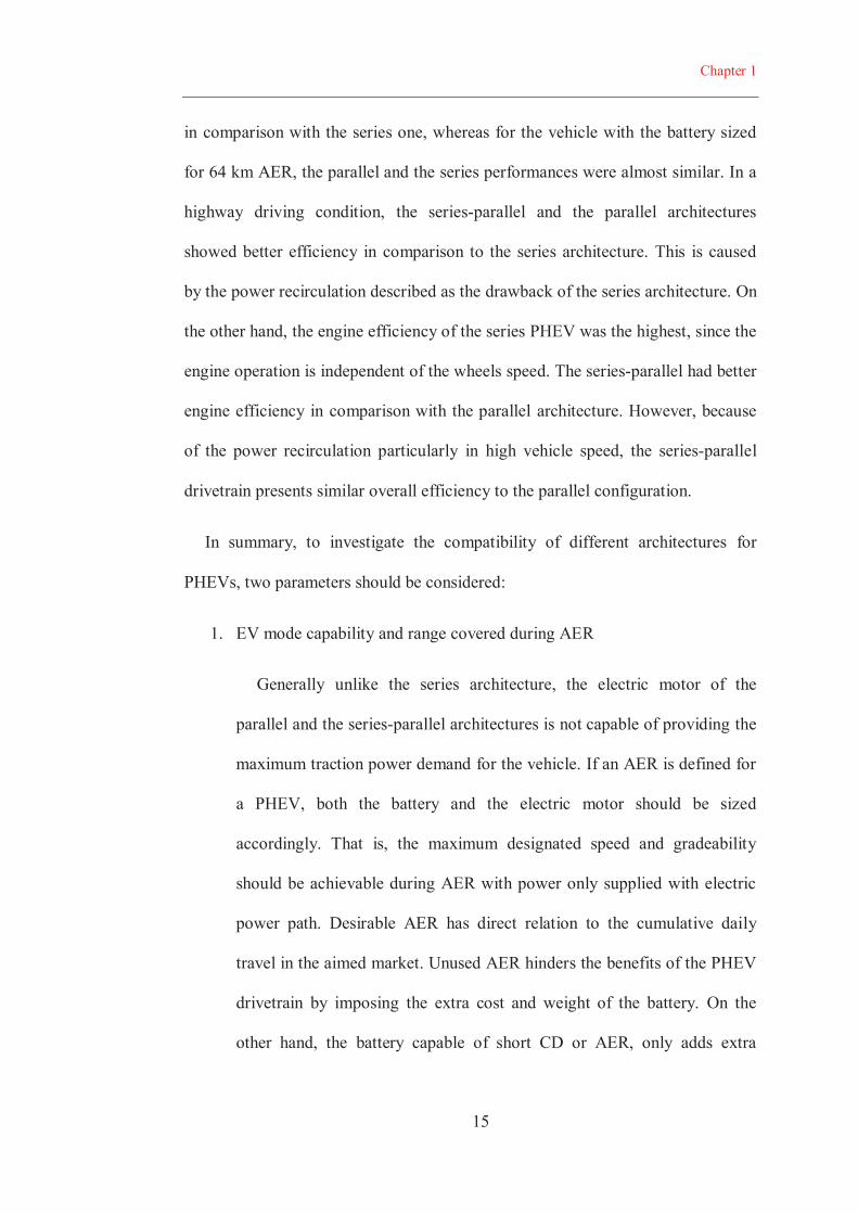
In summary, to investigate the compatibility of different architectures for
PHEVs, two parameters should be considered:
1. EV mode capability and range covered during AER
Generally unlike the series architecture, the electric motor of the
parallel and the series-parallel architectures is not capable of providing the
maximum traction power demand for the vehicle. If an AER is defined for
a PHEV, both the battery and the electric motor should be sized
accordingly. That is, the maximum designated speed and gradeability
should be achievable during AER with power only supplied with electric
power path. Desirable AER has direct relation to the cumulative daily
travel in the aimed market. Unused AER hinders the benefits of the PHEV
drivetrain by imposing the extra cost and weight of the battery. On the
other hand, the battery capable of short CD or AER, only adds extra
Chapter 1
16
weight for a long CS mode operation of the vehicle during longer
journeys.
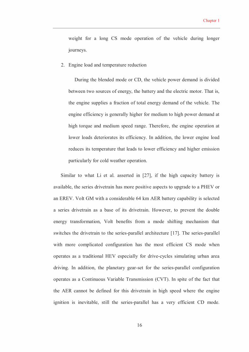
2. Engine load and temperature reduction
During the blended mode or CD, the vehicle power demand is divided
between two sources of energy, the battery and the electric motor. That is,
the engine supplies a fraction of total energy demand of the vehicle. The
engine efficiency is generally higher for medium to high power demand at
high torque and medium speed range. Therefore, the engine operation at
lower loads deteriorates its efficiency. In addition, the lower engine load
reduces its temperature that leads to lower efficiency and higher emission
particularly for cold weather operation.
Similar to what Li et al. asserted in [27], if the high capacity battery is
available, the series drivetrain has more positive aspects to upgrade to a PHEV or
an EREV. Volt GM with a considerable 64 km AER battery capability is selected
a series drivetrain as a base of its drivetrain. However, to prevent the double
energy transformation, Volt benefits from a mode shifting mechanism that
switches the drivetrain to the series-parallel architecture [17]. The series-parallel
with more complicated configuration has the most efficient CS mode when
operates as a traditional HEV especially for drive-cycles simulating urban area
driving. In addition, the planetary gear-set for the series-parallel configuration
operates as a Continuous Variable Transmission (CVT). In spite of the fact that
the AER cannot be defined for this drivetrain in high speed where the engine
ignition is inevitable, still the series-parallel has a very efficient CD mode.
Chapter 1
17
Therefore, it can be concluded that for PHEVs with a smaller battery similar to
Prius PHEV, the series-parallel architecture is a suitable choice.
The overall performance of PHEVs dramatically depends on the driving style
and conditions when compared to the conventional HEVs. This is due to the
added weight of a large battery, when depleted during the AER or CD modes, is
just an extra weight. Also, the reduced load of the engine leads to its lower
efficiency when compared to conventional HEVs [25].
1.4 PATHWAY FOR BETTER FUEL ECONOMY
Improvements in: (i) well-to-tank, (ii) wheel-to-miles, and (iii) tank-to-wheel
efficiencies are three possible approaches to reduce the fuel consumption of
vehicles [1, 2].
Available techniques to improve the tank-to-wheel efficiency of vehicles are
listed below:
1) Hybridization
2) Engine efficiency improvement
Turbocharging and supercharging
Direct injection
Low friction lubrication
Variable valve timing, variable compression ratio
Electric accessories (water pump, oil pump, air-condition
compressor)
3) Transmission
Chapter 1
18
Manual transmission
Continuous variable transmission (CVT)
Electronic continuous variable transmission (ECVT)
4) Vehicle
Aerodynamic improvement
Low rolling resistance tires
High strength/ low weight alloy and carbon fibre structure
The engine size has significant effect on the fuel economy of the vehicle. For
the same power demand from the engine, the efficiency of smaller engines is
generally higher. The reason is that the oversized engines are chosen for getting
the maximum power demand of conventional vehicles. Drivability, acceleration,
gradeability, and towing capacity design targets define the maximum power
demand of vehicles. For HEVs or especially for PHEVs in which a powerful
battery and an electric motor are available in the powertrain, depending to the
architecture, the maximum power demand of the vehicle is supplied with an
electric energy path in addition of the engine path. A downsized engine only
provides the average power demand of the vehicle that is significantly lower than
the designated maximum power capability of the drivetrain. The maximum power
of the engine is sized equal to the power demand of the vehicle for cruising at
designed maximum speed.
This research focuses on the improvement of the tank-to-wheel efficiency,
assuming a predefined component selection for the propulsion system. The
opportunities offered by a chosen drivetrain is realised by developing an
appropriate EMS. In the following notes, the concept of the fuel consumption of
Chapter 1
19
the vehicle is reviewed and the important parameters for the efficiency of PHEVs
are highlighted.
1.4.1 Efficiency of PHEV components
The fuel economy and the maximum AER covered by a fully charged battery
are dependent to the efficiency of each of the PHEV individual components. As
mentioned before, it is assumed that the components of PHEVs are chosen and the
aim of this research is to develop an appropriate EMS to maximise the total
efficiency of the vehicle. This requires a comprehensive understanding of the
components efficiency to avoid their low efficiency operation region by means of
the degree of freedom that the hybrid system offers for selection of different
energy paths.
Engine efficiency
The internal combustion (IC) engine is the most popular main source of power
for vehicles. The term engine in this research mainly refers to the Spark Ignited
(SI) engines. However, the developed methods in this research are similarly
applicable to other types of engines like Compression Ignition (CI), two-stroke,
Wankel rotary, and Stirling engines. Brake Specific Fuel Consumption (BSFC) is
the term defined to show how efficiently an engine transforms fuel energy to the
usable mechanical power at the crankshaft. BSFC is defined as the fuel flow rate
per useful power output and generally is in unit.
Chapter 1
20
is the fuel flow rate and is the engine useful power output. The
efficiency of the engine is defined as the ratio of the engine power to the amount
of fuel energy supplied.
where is the fuel lower heating value.
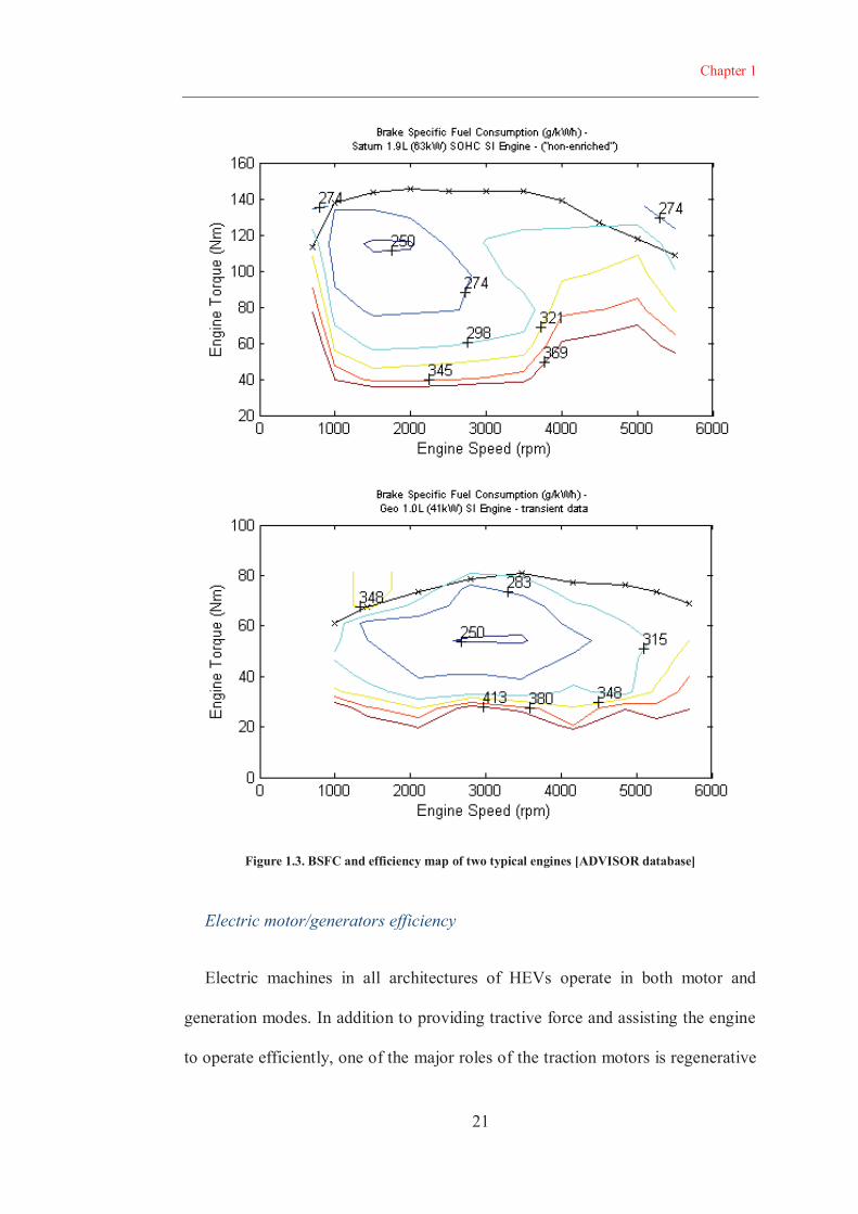
The efficiency of engine varies widely with its speed and torque. Among all
applicable operation points of an engine, the most efficient region of engine
operation is generally located at the middle range speed and high torque. BSFC
and efficiency map of a typical engine is depicted in Figure 1.3. Avoiding low
efficiency regions of the engine is almost part of all HEVs and PHEVs EMSs. The
EV mode at low vehicle speed and power-boost with electric motor when high
power required from the drivetrain are well-known approaches to avoid the low
efficiency operation of the engine for HEVs.
Chapter 1
21
Figure 1.3. BSFC and efficiency map of two typical engines [ADVISOR database]
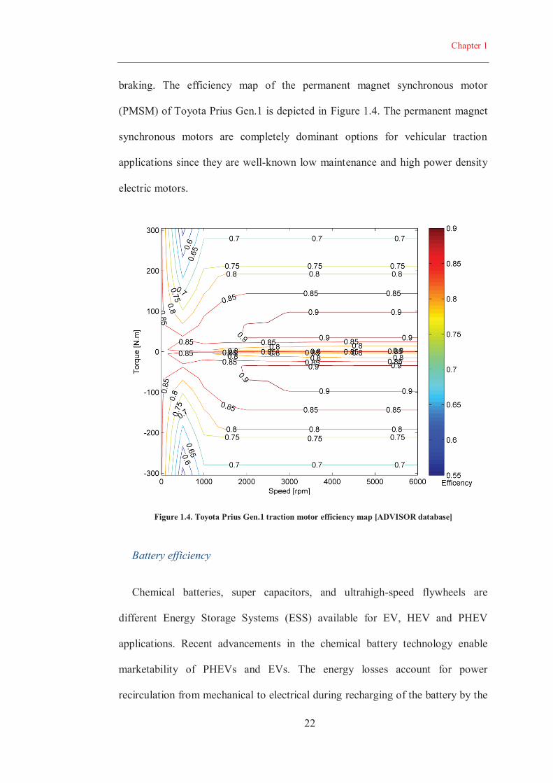
Electric motor/generators efficiency
Electric machines in all architectures of HEVs operate in both motor and
generation modes. In addition to providing tractive force and assisting the engine
to operate efficiently, one of the major roles of the traction motors is regenerative
Chapter 1
22
braking. The efficiency map of the permanent magnet synchronous motor
(PMSM) of Toyota Prius Gen.1 is depicted in Figure 1.4. The permanent magnet
synchronous motors are completely dominant options for vehicular traction
applications since they are well-known low maintenance and high power density
electric motors.
Figure 1.4. Toyota Prius Gen.1 traction motor efficiency map [ADVISOR database]
Battery efficiency
Chemical batteries, super capacitors, and ultrahigh-speed flywheels are
different Energy Storage Systems (ESS) available for EV, HEV and PHEV
applications. Recent advancements in the chemical battery technology enable
marketability of PHEVs and EVs. The energy losses account for power
recirculation from mechanical to electrical during recharging of the battery by the
Chapter 1
23
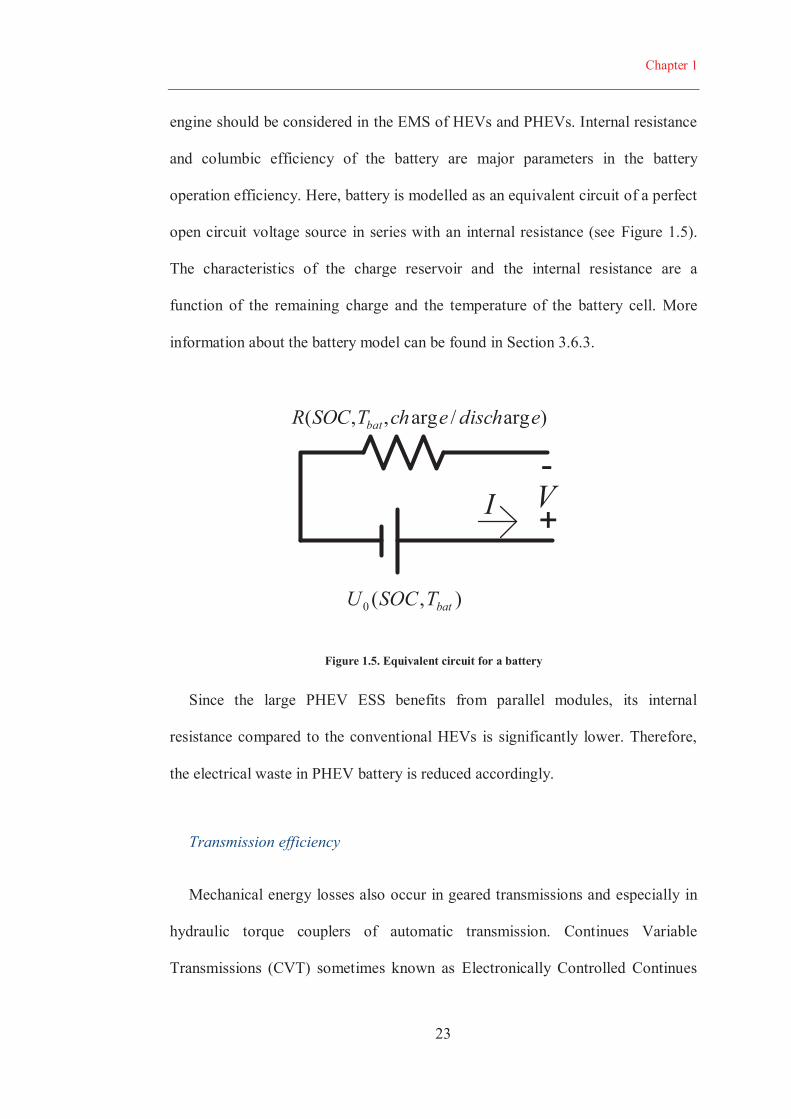
engine should be considered in the EMS of HEVs and PHEVs. Internal resistance
and columbic efficiency of the battery are major parameters in the battery
operation efficiency. Here, battery is modelled as an equivalent circuit of a perfect
open circuit voltage source in series with an internal resistance (see Figure 1.5).
The characteristics of the charge reservoir and the internal resistance are a
function of the remaining charge and the temperature of the battery cell. More
information about the battery model can be found in Section 3.6.3.
),(0 batTSOCU
)arg/arg,,( edischechTSOCR bat
I-+V
Figure 1.5. Equivalent circuit for a battery
Since the large PHEV ESS benefits from parallel modules, its internal
resistance compared to the conventional HEVs is significantly lower. Therefore,
the electrical waste in PHEV battery is reduced accordingly.
Transmission efficiency
Mechanical energy losses also occur in geared transmissions and especially in
hydraulic torque couplers of automatic transmission. Continues Variable
Transmissions (CVT) sometimes known as Electronically Controlled Continues
Chapter 1
24
Variable Transmissions (ECVT) is dominant in power-split type hybrid systems.
Most of the commercialized HEVs and PHEVs benefit from a planetary-gear-set
power split system. Geared transmissions generally have very high efficiency.
Gear ratio is the only controllable parameter affecting the vehicle performance by
changing the engine or electric machines operation points. This can be controlled
by part of EMS responsible for selection of the optimum engine to wheel speed
ratio.
Power electronics efficiency
The efficiency of the power electronics has important role particularly for
PHEVs in which a significant share of the required traction energy is provided
electrically. In terms of the energy management strategy of PHEVs, there is no
meaningful control over the power electronics efficiency. The detail of power
electronics of PHEVs’ converters and inverters is out of the scope of this research.
1.4.2 Auxiliary loads
Auxiliary loads have a significant role on energy consumption of vehicles. For
instance, the air conditioning (AC) required power even outweighs the losses
accounted for aerodynamic, rolling resistances, or driveline losses. The power
required for the AC equals the amount of power required to run the vehicle at
steady state speed of 56 km/hr [31]. Tests show that the AC contributes 37% of
the emission of the vehicle over the US Supplemental Federal Test Procedure
[32].
Chapter 1
25
The effect of the auxiliary load is even higher for more fuel-efficient vehicles
like HEVs and PHEVs. For instance, the Honda Insight fuel consumption is
increased by 46% when the AC is used. The study by Johnson showed that the US
uses 27 billion litres of gasoline every year for the AC in vehicles, equivalent to
6% of the domestic petrol consumption or 10% of US imported crude oil. [31].
Since it is completely likely for HEVs and PHEVs that the engine turns off for
a long period, many auxiliary loads should be provided electrically by the battery.
Therefore, the mechanical connection between the engine and the auxiliaries is
replaced by electrically powered components. Electric water pump, oil pump,
hydraulic steering fluid pump, brake booster vacuum pump, and AC compressor
electric motor are some examples. There is a large difference between the HEVs
and PHEVs auxiliary loads that arises from the very long engine-off mode or the
AER capability of PHEVs. The engine in HEVs is the sole energy source assuring
that hot water is always available for cabin heating for cold seasons. However, the
electric cabin heaters must be employed to satisfy passengers comfort. This adds
an extra auxiliary load which is conventionally supplied free of cost from the
engine coolant.
1.4.3 Energy management strategy
An energy management strategy is a control rule that is pre-set in the vehicle
controller and commands the operation of the drivetrain components. The vehicle
controller receives the operation commands from the driver and the feedback from
the drivetrain and all the components, and then makes decisions to use proper
operation point for the drivetrain components. Obviously, the performance of the
Chapter 1
26
drivetrain relies mainly on the control quality in which the energy management
strategy plays a crucial role. This thesis focuses directly on the optimization of
EMS of PHEVs. Therefore, a complete chapter is dedicated to describe the
important concepts in the EMS of HEVs and PHEVs. The full literature review on
the EMSs is outlined in Chapter 2.
1.5 RESEARCH AIM, OBJECTIVES AND CONTRIBUTIONS
The main aim of this research is to improve PHEVs’ fuel consumption by
developing an optimal energy management strategy (EMS) for the vehicles.
Emissions reduction and saving the state of the health of the battery are also two
secondary objectives of the research. It is assumed that the architecture and sizing
of the vehicle components are already chosen. The EMS tries to harness the
maximum benefit of the drivetrain potentials and specially the extra energy source
that the grid-charged battery provides. Therefore, a charge management strategy is
incorporated into the EMS.
As described in Section 1.4, the pathway for better fuel economy, a
comprehensive knowledge of different environmental and vehicle internal
characteristics is required to fulfil the aim of this study. The knowledge of future
driving patterns for the journey is crucial to benefit optimally from the extra
energy source available in the battery. The blended mode EMSs are only feasible
when the driving pattern is known. The driving pattern consists of the drive-cycle
and a comprehensive knowledge of the environmental impact on the power
demand and the performance of the vehicle components. Particularly, PHEVs are
more sensitive to the temperature noise-factor. Temperature alters the power
Chapter 1
27
demand of the vehicle when the AC or the cabin heater operation is required.
Besides, the performance of the vehicle components is influenced by temperature.
Therefore, the integration of thermal management and the EMS of PHEVs is
required to address the aim of the research.
The main contributions of this thesis are outlined as follows:
The effects of noise factors on the drivetrain power demand and the
performance are investigated by introducing the concept of the power-
cycle in place of the drive-cycle for a journey.
An applicable solution for developing a library of power-cycles inside the
vehicle is introduced to potentially make the noise factors predictable. By
considering the noise factors and the power-cycle library, the future
power-cycle is predictable more accurately.
The effect of temperature on the performance of PHEV components and
its significance on optimal energy management strategies are identified
and discussed.
An easily implementable semi-optimised rule-based EMS for a known
power-cycle is proposed. The effect of the temperature noise factor on the
engine performance is also considered for the rule-based EMS.
A globally optimised EMS based on the theory of dynamic programming
(DP) is developed. It investigates the effect of temperature on the optimal
charge depleting trajectory of PHEVs for a predefined journey. The
optimal charge trajectory coincides with an engine temperature trajectory
which guarantees the optimal engine operation and maximum availability
Chapter 1
28
of engine hot water for cabin heating while satisfying the complete charge
depleting constraint.
A practical approach to employ the optimal charge trajectory for
calibrating a real-time rule based EMS is proposed.
1.6 OUTLINE OF THE THESIS
This thesis is organized as follows:
Chapter 2 provides a comprehensive literature review on energy management
strategies of HEVs and exclusively PHEVs.
Chapter 3 describes the modelling of the vehicle and presents a thermal model
of the engine required for evaluation of PHEVs performance considering the
temperature noise factor.
Chapter 4 introduces different noise factors which influence both the power
demand of the vehicle and the operation performance of the powertrain
components. Particularly, the temperature noise factor is highlighted since the
PHEVs performance is more sensitive to temperature compared to the
conventional HEVs. In addition, a library based prediction of the future power-
cycle, necessary for optimal charge management of PHEV, is characterized.
Chapter 5 presents a new rule-based EMS for a known power-cycle. The EMS
also considers the effect of the temperature noise factor on engine cold-factor
penalty.

Chapter 1
29
Chapter 6 describes the numerical optimization method used to implement the
optimal EMS. A new EMS with the dynamic modelling approach based on the
theory of dynamic programming (DP) is introduced.
Finally, Chapter 7 provides the concluding remarks and suggests the future
works.
30
CHAPTER 2
REVIEW ON ENERGY MANAGEMENT STRATEGIES FOR HEVS AND PHEVS
2.1 INTRODUCTION
In all type of HEVs or PHEVs, an energy management strategy (EMS) must
determine how to fulfil the power demand of the driver in an efficient manner
from different energy paths available in the hybrid system. The main objective of
the energy management strategies is generally the reduction of fuel/electricity
consumption and emission while considering drivability requirement and
components operation restrictions and characteristics. This chapter provides a
Chapter 2
31
review on classification of energy management strategies employed for HEVs and
PHEVs, with an emphasis on the recent literature on the EMS of PHEVs.
2.2 POWER, ENERGY, AND CHARGE MANAGEMENT STRATEGY
As described in Chapter 1, an EMS is a control rule that is pre-set in the
vehicle controller, and that commands the operation of drivetrain components [1].
The terms “energy management strategy”, “power management strategy”, and
“supervisory control strategy” are commonly used in similar context in HEV and
PHEV literature. Nevertheless, in this thesis two terms “energy management
strategy” and “power management strategy” are distinguished. In power
management strategy of conventional HEVs, the controller goal is to maintain
optimal operation of the powertrain for supplying a specific power demand as
well as sustaining the battery state of charge (SOC) [33]. In PHEVs, however, the
large battery has the role of both load levelling and energy source. Therefore, it is
acceptable if the battery SOC reaches the minimum applicable range. The
difference between the concepts of energy management and power management
are more distinguished in PHEVs control strategies as both the engine and the
battery are the sources of energy unlike HEVs in which the battery energy is also
supplied by the engine [34]. The available charge in PHEVs’ battery, generally a
battery, adds more flexibility to the EMS of PHEVs in distributing load between
the engine and the battery compared to conventional HEVs. A charge
management strategy should be incorporated into the EMS of PHEVs. The charge
management strategy in PHEVs defines how to share the available ESS energy
during a journey to optimally utilize it for improving the performance of the
Chapter 2
32
vehicle [35]. On the other hand, power management is generally concerned with
how to split the drivetrain power demand between the two power sources to
achieve the best performance in a real-time fashion.
2.2.1 PHEV operation modes
Brief description of PHEV operation modes is outlined in Section 1.3.2. The
charge management of a PHEV is incorporated into the EMS of PHEV, and
defines the vehicle operation mode. The simplest energy management of PHEVs
is to run the vehicle on the CD or if possible on the EV mode until the battery
depletes to a minimum applicable SOC. This stage is referred to as electric vehicle
(EV) mode and the range covered is named all electric range (AER).
Subsequently, the vehicle operates like a conventional HEV in the charge
sustaining (CS) mode to stabilize the SOC. The advantage of the AER followed
by the CS strategy is the maximum consumption of stored electric energy which is
relatively cheaper before the vehicle reaches its destination with available
recharging facilities.
Another energy management strategy, which is known as blended mode, uses
both the battery and the engine simultaneously for vehicle propulsion to achieve
higher efficiency as the available energy in the battery could help provide more
efficient load levelling in the hybrid system. Different researchers have developed
different blended mode EMS strategies, since they are considerably related to the
architecture and the components sizing of a specific PHEV. Specially, in the
parallel and the series-parallel architectures, the blended mode is inevitable
because of the drivetrain mechanical restrictions and components sizing [13, 36-

Chapter 2
33
39]. An appropriate powertrain load split between the battery and the engine
energy sources is therefore an important issue in developing the blended mode
strategies, as reaching the destination with surplus electric energy sacrifices the
benefit of availability of large and expensive battery on-board of PHEVs. The
schematic illustration of the PHEVs operation modes is depicted in Figure 2.1.
SOC
Time
CD- Blended ModeAER- EV Mode
CS Mode
Figure 2.1. PHEV operation modes
2.3 CLASSIFICATION OF ENERGY MANAGEMENT STRATEGIES
The full classification of the control problem of the EMS for HEVs and PHEVs
has been outlined in the literature [12, 33, 40-42]. The literature provides a
number of approaches for the EMS of HEVs, many equally applicable to both
plug-in and conventional (i.e., non plug-in) HEVs. The number of publications
about the EMS of PHEVs is relatively lower than that of the HEVs. The control
problem for the EMS of HEVs and PHEVs is generally grouped into two
categories: (i) rule-based controllers and (ii) optimization-based controllers [41].
Chapter 2
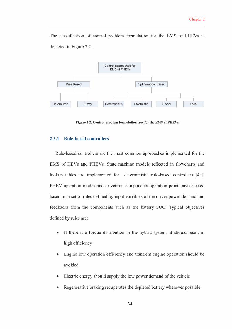
34
The classification of control problem formulation for the EMS of PHEVs is
depicted in Figure 2.2.
Control approaches forEMS of PHEVs
Rule Based Optimization Based
Determined Fuzzy LocalGlobalStochasticDeterministic
Figure 2.2. Control problem formulation tree for the EMS of PHEVs
2.3.1 Rule-based controllers
Rule-based controllers are the most common approaches implemented for the
EMS of HEVs and PHEVs. State machine models reflected in flowcharts and
lookup tables are implemented for deterministic rule-based controllers [43].
PHEV operation modes and drivetrain components operation points are selected
based on a set of rules defined by input variables of the driver power demand and
feedbacks from the components such as the battery SOC. Typical objectives
defined by rules are:
If there is a torque distribution in the hybrid system, it should result in
high efficiency
Engine low operation efficiency and transient engine operation should be
avoided
Electric energy should supply the low power demand of the vehicle
Regenerative braking recuperates the depleted battery whenever possible
Chapter 2
35
Charge sustaining limits for HEVs and charge depleting limits for PHEVs
are enforced with the controller
Fuzzy controllers are also another rule-based approach for designing the EMS,
and are more efficient compared to deterministic rule-based controllers [44-46].
The main advantage of the rule-based controllers is that they are based on
engineering intuition and physical tests and are generally easily implementable.
Unfortunately, the behaviour of the rule-based controllers extremely depends on
the selected thresholds for change of states or in case of the fuzzy controllers the
definition of membership functions. The driving condition and the driver
behaviour could substantially alter the optimal defined thresholds and
membership functions. A blend of pattern recognition and fuzzy logic was
proposed by Langari and Won for a HEV [47, 48].
2.3.2 Optimization based controllers
Optimization based controllers are identified based on the mathematical
modelling approach selected to formulate the HEV or PHEV energy management
control problem. Optimization based controllers can be classified into two
branches: local vs. global optimization and deterministic vs. stochastic
optimization (see Figure 2.2)
Local vs. global optimization
Performance and fuel economy of a PHEV depend on its efficiency in all
segments of a journey. Local optimization approaches have a major drawback that
Chapter 2
36
is they cannot find the global optimum solution resulting in non-optimal operation
of HEVs or PHEVs for the whole journey [2, 25, 33-35, 41]. Particularly for the
EMS of PHEVs, the optimal charge management requires insight about the
driving pattern of the vehicle from the beginning to the end of journey. It is
mathematically possible to find the optimal solution for the EMS of PHEVs if
accurate information about the trip like drive-cycle and accessories power demand
is available in advance to formulate the optimal control problem. Indeed, a correct
formulation of the vehicle model is the perquisite to solve the optimal control
problem. Using historic driving patterns, GPS, vehicle-to-vehicle, and
vehicle-to-infrastructure communication facilitate more accurate prediction of
driving scenario [34, 49-52]. In the absence of any information about the vehicle
trip, the local optimization approaches are the only viable solutions.
Global optimization based controller for EMS
Dynamic programming (DP) is one of the most well-known and powerful
optimization tools to solve complex control problems. Dynamic programming is
known as both a globally optimised and a deterministic energy management
strategy. Dynamic programing is a globally optimal approach which can find the
best charge depleting profile, also can act as the benchmark for other EMSs of
PHEVs. It gives the best possible solution for the control problem with respect to
the used discretization of time, state space, and inputs. Dynamic programming
suffers from the curse of dimensionality, which means that the computational time
increases exponentially with an increase in state variables. Its key disadvantage is
the high computational effort which is opposed to its real-time implementation for
online control of a vehicle [49, 53-60]. Since charge management is only
Chapter 2
37
applicable when the whole journey is considered over optimization horizon, it is
thus necessary to predict the driving pattern of the vehicle in advance to formulate
the optimal control problem of the EMS of PHEVs.
Local optimization based controller for EMS
Local optimization methods are somewhat similar to the rule-based controllers
as only the current operation of the hybrid system is optimised. Since the EMS of
PHEV should incorporate a charge management strategy alongside an online
power management strategy, the local optimization based controllers are not
appropriate to achieve the maximum benefit of having a large battery on board. A
well-known locally optimised controller approach adopted for on-line control of
HEVs is equivalent consumption minimization strategy (ECMS) [2, 61-64]. For
the ECMS, the electricity consumption is converted to an equivalent amount of
fuel consumption, and then the EMS tries to minimise the equivalent fuel
consumption in an on-line fashion. The ECMS is a deterministic approach that
can be derived based on Pontryagin’s minimum principle introduced in [65]. The
equivalence based control algorithms evaluate which combination of the traction
sources is more appropriate for the current power demand. Generally, ECMS is
developed for parallel hybrid architecture in the literature. The combined
equivalent power is defined by Eq. 2-1.
where is equivalence factor and is a penalty defined to prevent frequent
change of condition like gear shifting or rapid changes of engine velocity. If
Chapter 2
38
increases the cost of providing power demand of the vehicle from electric energy
path rises proportionally compared to the engine energy path. The term
equivalence factor , , comes from the fact that in HEVs all energy comes
ultimately from the fuel, the battery charge or discharge are translated respectively
into equivalent fuel consumption or equivalent fuel savings. The knowledge of
power-cycle is required to tune the equivalence factor, based on the past and
future driving condition to satisfy the battery charge trajectory and boundary
limitations [55, 66]. Another approach is to use a PI controller which changes
aiming for a given target battery charge. This adapting process of is also known
as A-ECMS [67]. The disadvantage of A-ECMS is its sub-optimality compared to
the global optimal approaches. As the cost function based on the equivalent
power, is developed locally, consideration of the slow dynamic phenomena
like temperature are not practically implementable for this approach.
Deterministic vs. stochastic optimization
Deterministic systems consistently provide a similar output to a set of input
variables. As mentioned before, DP is a deterministic optimization approach to
find a globally optimised EMS. Stochastic dynamic programming, however, deals
with the optimization problems which involve some uncertainty and random
elements. Stochastic dynamic programming (SDP) is appealing for optimization
of EMSs over a probabilistic distribution of power-cycles, rather than a single
cycle [68-74]. Unlike deterministic DP, the optimization process is performed on
a class of trajectories from an underlying Markov chain power-cycle generator
rather than a single predefined power-cycle. If this stochastic process is able to
Chapter 2
39
well define the journey characteristics, the optimal EMS could be developed
based on it. Since the process of Markov chain is time invariant, the assumption is
that the vehicle will continue to drive forever which is not appealing for charge
management of PHEVs. As described before, charge management has an
important role in the EMS of long electric range PHEVs. Therefore, SDP suits
better for HEVs or PHEVs in which the battery and motor are incapable of the
AER or the EV mode.
2.4 EMSS EXCLUSIVELY DEVELOPED FOR PHEVS
In comparison to the literature of the HEVs’ control strategies, there are a
limited number of publications which investigate the EMS of PHEVs. In the
following notes, some of the approaches that exclusively address the EMS of
PHEVs are outlined.
Gao et al. suggested two different rule-based EV-CS and blended EMSs for a
PHEV with the parallel architecture [13, 36]. They also suggested a manual
shifting option between the EV and the CS for driver. In this rule-based strategy,
the engine is constrained to operate around its efficient region defined by two
minimum and maximum torque boundaries in the engine efficiency map. The
engine is controlled as that no surplus energy remains to charge the battery to
prevent charging and discharging power recirculation wastes. When the required
torque is higher than the top torque boundary, the remaining power demand is
supplied by the electric motor. The engine solely propels the wheel if the
demanded torque from the engine is between the boundaries of the defined
efficient region. The engine is turned off when the torque demand is below the
Chapter 2
40
bottom torque boundary and the vehicle runs in purely in the EV mode. In this
approach, it is assumed that there is no information available about the trip
duration and length. Therefore, when vehicle operates in the blended mode, it is
possible to reach destination with surplus in battery energy for short trips.
Whereas, the EV-CS EMS uses relatively cheaper battery energy in place to petrol
for the same trip. Therefore, this approach does not provide higher fuel economy
for all situations.
Sharer et al. in [38] simulated and compared four different blended rule-based
EMSs for a series-parallel PHEV with 16 km AER battery in PSAT for a vehicle
with similar component sizing of the Freyermuth et al. model explained in
reference [30]. The four EMSs are named as:
Electric vehicle/charge sustaining (EV/CS)
Differential engine power
Full engine power
Optimal engine power
In “EV/CS” EMS, the engine only turns on when the power demand is higher
than the available power of the battery until the battery depletes to its minimum
applicable SOC. “Differential engine power” EMS is similar to the EV/CS but
the engine-turn-on threshold is defined lower than the maximum applicable power
of the battery. In “full engine power” EMS, if the engine turns on it will supply all
the power demand of the vehicle and no power will be drained from the battery.
The aim of this strategy is to force the engine to operate at higher loads and
consequently with higher efficiency. In “optimal engine power” EMS, the engine
Chapter 2
41
is restricted to operate close to the peak efficiency point of the engine. For
different predetermined journey distances, the engine-start threshold can be
derived and calibrated by simulation. In other words, for longer journeys to
continue further in the CD mode before entering the CS mode, the engine-turn-on
threshold should be reduced. The concept behind this EMS is to force the engine
to operate and ignite in higher average efficiencies during the journey as much as
possible by saving electric energy for low power demand sections of drive-cycles.
The simulation results prove that the “differential engine power” EMS has a
similar overall efficiency with respect to “EV/CS” EMS since the engine
operation in low loads deteriorates the vehicle overall fuel economy. “Full engine
power” EMS resulted in the best fuel economy with about 9% improvement even
more than the “optimal engine power” EMS. Although the engine operates more
efficiently in the “optimal engine power” EMS, the overall efficiency is reduced
due to the effect of power recirculation and efficiency chain. The interesting result
was that the “optimum engine power” EMS produced no significant improvement
and even sometimes deteriorated the efficiency for some trip distances compared
to the EV/CS EMS [38].
The deterministic dynamic programming (DP) approach was employed by
Gong et al. to force the battery to get fully depleted exactly at the end of journey.
The global optimization by means of the DP algorithm offered significant
efficiency improvement in comparison with the EV/CS EMS. As the DP is a
deterministic approach, the trip information as a priori is required. Therefore, trip
simulation with GPS and GIS information is introduced in this paper [49].
Chapter 2
42
A stochastic optimal approach for the power management of PHEVs was
suggested by Moura et al. to optimise a series-parallel drivetrain for a
probabilistic distribution of many power-cycles, rather than a single one [69]. By
using a discrete-time Markov chain, the model of power-cycle was predicted.
Both fuel and electricity costs are considered in the defined cost function.
Consequently, the benefits of controlled charge depleting were explored.
As mentioned before, the number of available published works in the field of
EMS of PHEVs is quite limited. The effect of different noise factors on the EMS
of PHEVs still has many aspects to explore (see Chapter 4).
2.5 CONCLUSION
Among all the existing EMS approaches described in this chapter, two
different methods, (i) a rule-based/deterministic and (ii) an optimization-based
/deterministic, are selected in this research. The deterministic approaches are
selected because one of the major objectives of this research is the optimal charge
management of PHEVs. Hence, the prediction of power demand pattern during
the journey is a prerequisite for developing the deterministic methods. In addition,
to explore the effect of slow dynamic phenomena like temperature on the
performance of vehicle, deterministic methods are only feasible options. The rule-
based approaches are easily implementable while the optimization-
based/deterministic approaches provide the global optimal solution. The rule-
based/deterministic approach is presented in Chapter 5 and the optimization-
based/deterministic approach is introduced in Chapter 6.

43
CHAPTER 3
VEHICLE MODELLING
3.1 INTRODUCTION
In this thesis, vehicle modelling deals with mathematical representation of
physical reality of longitudinal dynamics of the vehicle. This chapter discusses the
modelling approach for the vehicle and its powertrain components. The level of
acceptable approximation in modelling process defines the efficiency of the
model. The more detailed is the mathematical modelling of the physical
dynamics, the more complex and timely is the simulation process. The models in
Chapter 3
44
this research are defined with the aim of solving the optimal control problem for
the energy management strategy of PHEVs to improve fuel efficiency and reduce
emissions. Therefore, the dynamic phenomena that are not related to the energy
efficiency of the vehicle are neglected.
In order to evaluate the fuel economy of the vehicle, it is necessary to
understand the energy flow in different powertrain components of the vehicle. In
this chapter, first the basics of the longitudinal dynamics of the vehicle is
introduced, then the characteristics of modelling and sizing of the powertrain
components are outlined.
3.2 LONGITUDINAL DYNAMICS OF VEHICLES
The loads and parameters that affect the longitudinal dynamics of a vehicle and
its load demand are depicted in Figure 3.1. The dynamic equation of the vehicle
along the longitudinal direction is as follows:
where is tractive effort, is mass of vehicle, is linear acceleration of
vehicle along longitudinal direction, are rolling, drag, and grading
resistances, respectively. The required traction power, , is derived from Eq. 3-1
as follows:
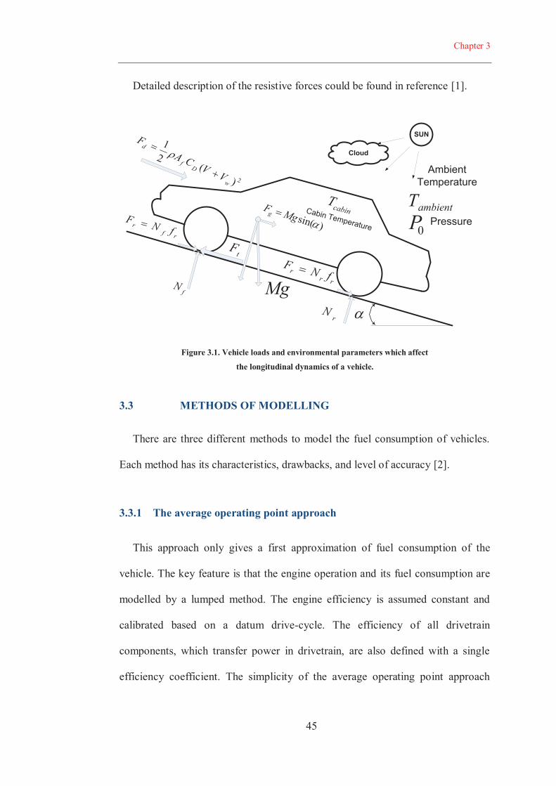
Chapter 3
45
Detailed description of the resistive forces could be found in reference [1].
Mg
)sin(
MgF
g
2)(
21
w
Df
d
VV
CAF
rfr fNF
rrr fNF
fN
rN
tF
SUN
ambientT0P
AmbientTemperature
Pressure
Cloud
cabinT
Cabin Temperature
Figure 3.1. Vehicle loads and environmental parameters which affect
the longitudinal dynamics of a vehicle.
3.3 METHODS OF MODELLING
There are three different methods to model the fuel consumption of vehicles.
Each method has its characteristics, drawbacks, and level of accuracy [2].
3.3.1 The average operating point approach
This approach only gives a first approximation of fuel consumption of the
vehicle. The key feature is that the engine operation and its fuel consumption are
modelled by a lumped method. The engine efficiency is assumed constant and
calibrated based on a datum drive-cycle. The efficiency of all drivetrain
components, which transfer power in drivetrain, are also defined with a single
efficiency coefficient. The simplicity of the average operating point approach
Chapter 3
46
makes it suitable for preliminary steps of finding fuel consumption and
performance investigation of vehicles. On the other hand, it has limited capability
for developing EMS for complex drivetrains like PHEVs in which the efficiency
of the components is significantly altered during different operation modes.
3.3.2 The quasi-static approach
In this approach, each simulation over a drive-cycle is divided into many time-
steps during which it is assumed that the vehicle velocity, acceleration, and any
other effective input variables remain constant. These time-steps should be short
enough to satisfy the quasi-static assumption. In this approach, to find the
efficiency of each component consisting of the engine, the electric
motor/generators, the battery, and the transmission components, instead of a
single efficiency coefficient an efficiency map is employed to reach more accurate
physical modelling. That is, based on the amount and components of power
(torque and angular velocity for mechanical parts or voltage and current for
electrical parts) are transferred from each powertrain nodes, the efficiency of each
component is derived from the efficiency maps for each time-step.
The quasi-static method is a powerful tool for development and analysis of the
EMS for all vehicular drivetrains under different levels of complexity with limited
numerical efforts. The main feature of the quasi-static modelling is its backward
formulation which requires the knowledge of the driving scenario in advance.
Therefore, this approach is not appropriate for feedback control or state events
simulation. In Section 3.4, descriptive characteristics of the forward and the
backward modelling approaches are explained.
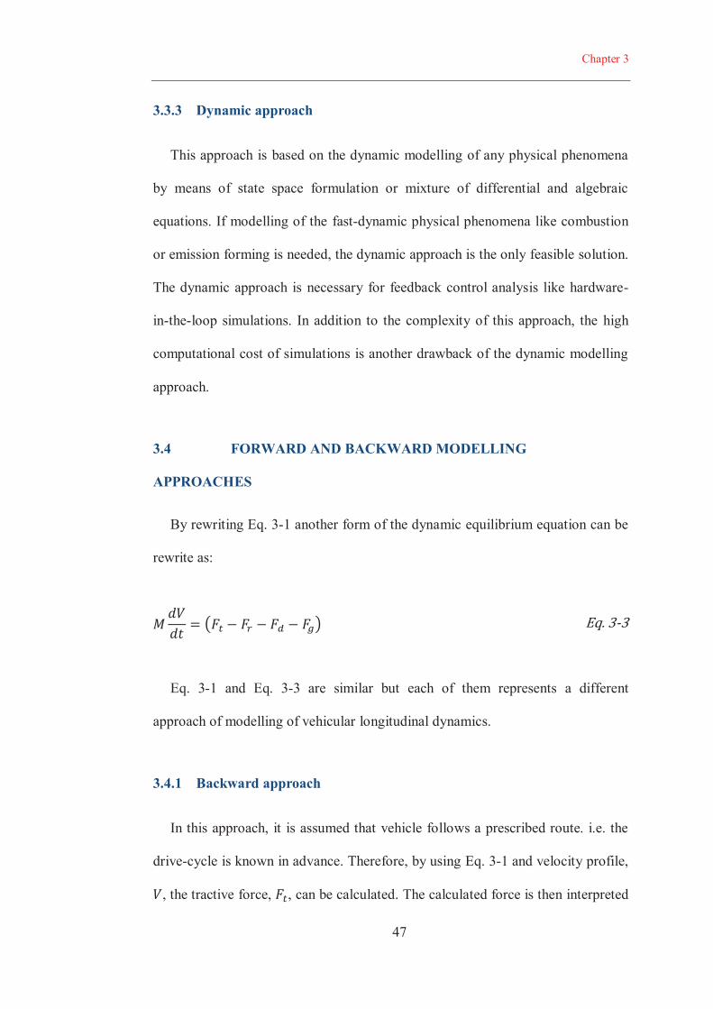
Chapter 3
47
3.3.3 Dynamic approach
This approach is based on the dynamic modelling of any physical phenomena
by means of state space formulation or mixture of differential and algebraic
equations. If modelling of the fast-dynamic physical phenomena like combustion
or emission forming is needed, the dynamic approach is the only feasible solution.
The dynamic approach is necessary for feedback control analysis like hardware-
in-the-loop simulations. In addition to the complexity of this approach, the high
computational cost of simulations is another drawback of the dynamic modelling
approach.
3.4 FORWARD AND BACKWARD MODELLING
APPROACHES
By rewriting Eq. 3-1 another form of the dynamic equilibrium equation can be
rewrite as:
Eq. 3-1 and Eq. 3-3 are similar but each of them represents a different
approach of modelling of vehicular longitudinal dynamics.
3.4.1 Backward approach
In this approach, it is assumed that vehicle follows a prescribed route. i.e. the
drive-cycle is known in advance. Therefore, by using Eq. 3-1 and velocity profile,
, the tractive force, , can be calculated. The calculated force is then interpreted
Chapter 3
48
to torque and angular velocity over the electric motor and the engine considering
the transmission ratios and wastes. As the calculation flows from force on the
wheel to downstream components in each time-step, the method is named as
backward approach. A combination of a quasi-static and backward approach is
generally a powerful tool for fuel-consumption prediction and development of
EMSs. Since the backward approach assures exact following of a prescribed
route, it is useful when the performance of the vehicle over benchmark drive-
cycles defined by authorities is the point of interest.
Since the backward quasi-static approaches are based on the static steady-state
efficiency maps, the transient behaviour of the components is neglected in this
approach.
3.4.2 Forward approach
In this approach, on the other hand, simulations start from a driver model.
Generally, a PID controller as a driver compares the actual and the required
vehicle speeds and provides the required control input commands. This input
command is then interpreted by EMS for the powertrain components of the
vehicle to minimise the error signal. The input commands transforms to torque
output from the engine and the electric motor. Then, the model based on the
dynamic Eq. 3-3 derives the real acceleration and velocity. The structure of the
forward approach makes it suitable for dynamic simulations.
Chapter 3
49
3.5 SIMULATION TOOLS
Fierce competition among automotive manufacturing entities puts significant
pressure on the companies to introduce new vehicle models to the market as soon
as possible. Almost all major automotive manufacturers have developed their own
simulation tools which mostly are unavailable to the public [75]. Mathematical
modelling has replaced many physical tests required for investigation of vehicle
performance and fuel consumption. Particularly, when performance comparison
and component sizing of newly developed HEVs and PHEVs is required,
simulations based on the mathematical modelling approaches are desirable.
The Mathworks products, Matlab and Simulink are the most popular platforms
for modelling of HEVs and PHEVs. Modelica also provides a causal modelling
language based of which the commercialized Dynasim Dymola modelling
platform has been developed. Some researches use it for their vehicular simulation
and modelling [76-78].
Advance Vehicle Simulator (ADVISOR) developed in National Renewable
Energy Laboratory, and Powertrain System Analysis Toolkit (PSAT) developed
in Argonne National Laboratory are two dominant simulation tools specifically
developed for advanced vehicles [79, 80]. Both ADVISOR and PSAT are
developed in Matlab/Simulink. ADVISOR is an empirical map-based simulation
tool that combines the vehicle dynamics model with the efficiency map of each
component to predict the vehicle performance. ADVISOR is a unique
combination of backward and forward simulation tool which calculates each
component operation parameters for a known drive-cycle based on the quasi-static
Chapter 3
50
assumption [79]. In contrast to ADVISOR, PSAT is a look-forward simulation
tool that calculates the powertrain states based on the driver input.
In addition to the commercial simulation and modelling tools, many
researchers have developed their own modelling tools to incorporate their
suggested control strategy into the simulation platforms [24, 81-84]. The major
reason is that the level of complexity of available commercial simulation tools
like ADVISOR or PSAT makes it hard to incorporate new models or controller
into them. Comprehensive understanding of the relationship between sub-models
and significant number of parameters is essential if one needs to incorporate some
new sub-models or controllers into the commercial simulation tools. In addition,
the developers of the commercial tools might intentionally restrict access to the
codes or sub-models. Nevertheless, this level of detailed modelling improves the
accuracy of simulation as the models are generally verified with physical test
conducted in well-equipped test facilities.
3.6 MODELLING APPROACH USED IN THIS WORK
Two different modelling approaches have been taken for this research. First,
the vehicle components are sized and modelled in a backward quasi-static
approach. As explained in the previous section, the backward quasi-static
modelling approach has beneficial characteristics for investigation of EMSs and
specially charge management to check the performance of the vehicle for a
complete journey. To verify the simulations and modelling approach in this
research, ADVISOR powertrain simulation tool is employed. ADVISOR
developed by National Renewable Energy Laboratory (NREL) [79]. In 2003
Chapter 3
51
(NREL) transferred a license to commercialize ADVISOR to AVL Powertrain
Engineering, Inc. [85]. ADVISOR provides a trusted, verified, and detail model of
the vehicle that assures accurate and close to reality simulation results.
The second modelling method that would be described in details in Chapter 6
is a dynamic approach based on the theory of dynamic programming. An inverse
powertrain model analogous to the quasi-static model of a PHEV is formulated as
an optimal control problem in dynamic programming to find the optimal charge
depleting trajectory and the EMS of the PHEV.
3.6.1 Drivetrain architecture and sizing of the sub-models
A model of EREV is developed for the serial powertrain architecture. The
basic characteristics of the considered vehicle are given in Table 3-1. The main
components of the vehicle are illustrated schematically in Figure 3.2. We have
tried to keep the sizing of the components similar to the published characteristics
of GM Volt. GM Volt is a 64 km EREV benefiting from a mode changing
architecture by means of a planetary gear set which can shift the vehicle
architecture from serial to series-parallel. In this mode, the engine could
mechanically transfer power to the final drive in higher speeds and power
demands. Also, it has two different EV modes in which the EV mode is shifted
from one electric motor drive to two electric motor drives in order to reduce the
losses in higher speeds and cruise operation [17]. This mode shifting capability is
not considered in the model of the vehicle used in this thesis, because the aim of
this research is merely the investigation of the effect of temperature on charge
Chapter 3
52
management of PHEVs which can be applied to all PHEVs regardless of their
drivetrain architecture.
The reason that an EREV with the series drivetrain is selected for this research
is that the influence of the temperature noise factor becomes more significant for
PHEVs with a large battery than those with a small battery. A large battery can
provide a larger portion of the total energy demand of the vehicle compared with a
small battery. When more electric energy is used instead of fuel to support the
wheel power demand, the engine would undesirably run cooler. Also, long EV
modes are major characteristics of EREVs which leads to the long cool-down
periods. Therefore, sensitivity of EREV to temperature noise factor is the worst
case scenario affected by temperature noise factor if a blended mode EMS is
operating the vehicle. Accordingly, this research focuses on the serial EREVs
having a large battery.
Moreover, the operation of the power split hybrid vehicles is highly influenced
by the dynamic of the planetary gear set. Therefore, this constraint leads to a
lower degree of freedom for the engine operation associated with the wheel power
demand. For instance, due to the dynamic restriction, the Prius PHEV cannot
operate in the EV mode at speeds higher than 100 km/hr. Also, it is necessary to
turn the engine on even at lower speeds if the maximum traction power, which is a
combination of electric motor and engine power, is required.
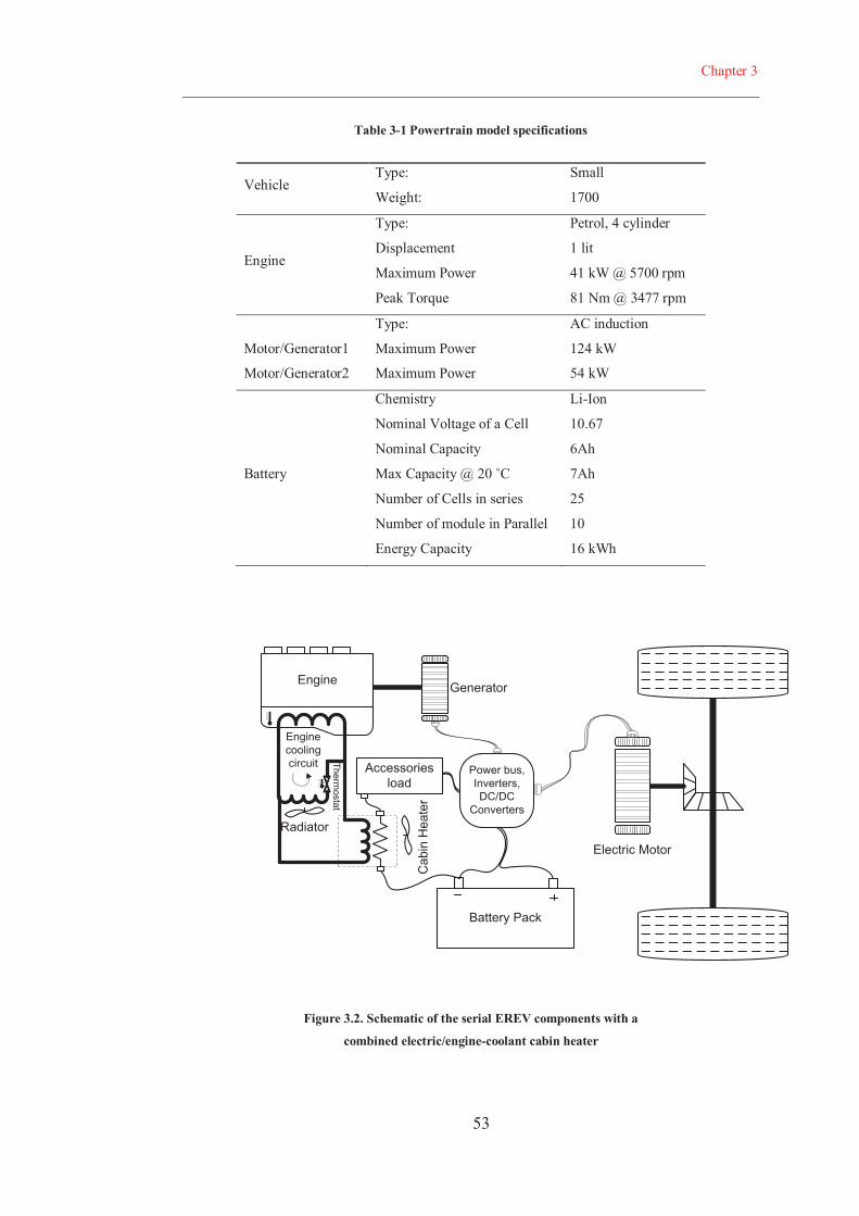
Chapter 3
53
Table 3-1 Powertrain model specifications
Vehicle Type:
Weight:
Small
1700
Engine
Type:
Displacement
Maximum Power
Peak Torque
Petrol, 4 cylinder
1 lit
41 kW @ 5700 rpm
81 Nm @ 3477 rpm
Motor/Generator1
Motor/Generator2
Type:
Maximum Power
Maximum Power
AC induction
124 kW
54 kW
Battery
Chemistry
Nominal Voltage of a Cell
Nominal Capacity
Max Capacity @ 20 ˚C
Number of Cells in series
Number of module in Parallel
Energy Capacity
Li-Ion
10.67
6Ah
7Ah
25
10
16 kWh
Electric Motor
Power bus,Inverters,DC/DC
Converters
Battery Pack
Engine Generator
Radiator
Enginecoolingcircuit Therm
ostat
Cab
inH
eate
r
Accessoriesload
Figure 3.2. Schematic of the serial EREV components with a
combined electric/engine-coolant cabin heater
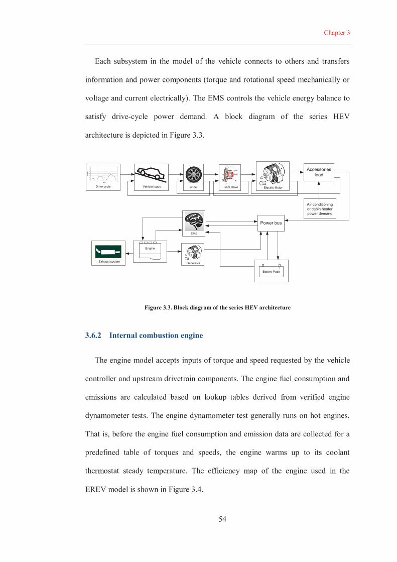
Chapter 3
54
Each subsystem in the model of the vehicle connects to others and transfers
information and power components (torque and rotational speed mechanically or
voltage and current electrically). The EMS controls the vehicle energy balance to
satisfy drive-cycle power demand. A block diagram of the series HEV
architecture is depicted in Figure 3.3.
Engine
zBattery Pack
Accessoriesload
Power bus
GeneratorExhaust system
EMS
Electric MotorFinal DrivewheelVehicle loadsDrive cycle
Air conditioningor cabin heaterpower demand
Figure 3.3. Block diagram of the series HEV architecture
3.6.2 Internal combustion engine
The engine model accepts inputs of torque and speed requested by the vehicle
controller and upstream drivetrain components. The engine fuel consumption and
emissions are calculated based on lookup tables derived from verified engine
dynamometer tests. The engine dynamometer test generally runs on hot engines.
That is, before the engine fuel consumption and emission data are collected for a
predefined table of torques and speeds, the engine warms up to its coolant
thermostat steady temperature. The efficiency map of the engine used in the
EREV model is shown in Figure 3.4.
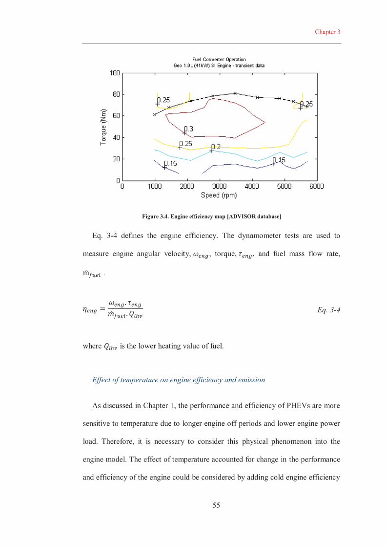
Chapter 3
55
Figure 3.4. Engine efficiency map [ADVISOR database]
Eq. 3-4 defines the engine efficiency. The dynamometer tests are used to
measure engine angular velocity, , torque, , and fuel mass flow rate,
.
Eq. 3-4
where is the lower heating value of fuel.
Effect of temperature on engine efficiency and emission
As discussed in Chapter 1, the performance and efficiency of PHEVs are more
sensitive to temperature due to longer engine off periods and lower engine power
load. Therefore, it is necessary to consider this physical phenomenon into the
engine model. The effect of temperature accounted for change in the performance
and efficiency of the engine could be considered by adding cold engine efficiency
Chapter 3
56
maps to engine model or mathematically formulating the cold-factor efficiency
penalty. The first option requires forced cold operation of the engine during
dynamometer tests and repeating them for adequate range of operation
temperatures. This option is more accurate as the engine efficiency is a dependent
function of its temperature, torque, and speed. However, this requires repeating
expensive tests to fully define the engine temperature correction factors.
In a mathematical modelling approach, the cold-to-hot engine fuel and
emissions penalties for SI engines have been investigated by Murrell et al. [86].
The correction factor is incorporated based on normalised engine temperature
factor, , which is related to the engine cooling system thermostat set point,
, and the coolant temperature, :
Eq. 3-5
where temperature is in centigrade degrees. The fuel and emissions are then
computed as follows based on, γ, and the engine performance in hot operation:
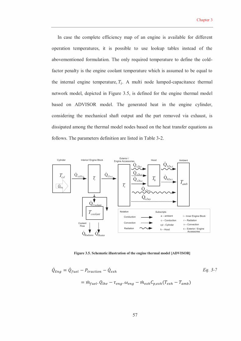
Chapter 3
57
In case the complete efficiency map of an engine is available for different
operation temperatures, it is possible to use lookup tables instead of the
abovementioned formulation. The only required temperature to define the cold-
factor penalty is the engine coolant temperature which is assumed to be equal to
the internal engine temperature, . A multi node lumped-capacitance thermal
network model, depicted in Figure 3.5, is defined for the engine thermal model
based on ADVISOR model. The generated heat in the engine cylinder,
considering the mechanical shaft output and the part removed via exhaust, is
dissipated among the thermal model nodes based on the heat transfer equations as
follows. The parameters definition are listed in Table 3-2.
`
Cylinder Interior/ Engine BlockExterior /
Engine Accessories Hood Ambient
cylTiT
xThT
ambT
coolantT
CoolantFlow
cyl2i,cQ i2x,cQx2h,cQ
CoolantQ
vx2h,Qrx2h,Q
rx2a,Q
vx2a,Q
vh2a,Q
rh2a,Q
Notation
Conduction
Convection
Radiation
Subscripts
cyl - Cylinder
i – Inner Engine Block
x – Exterior / EngineAccessories
h – Hood
a – ambient
RadiatorQ HeaterQ
c – Conduction
v – Convection
r – Radiation
EngQ
Figure 3.5. Schematic illustration of the engine thermal model [ADVISOR]
Eq. 3-7
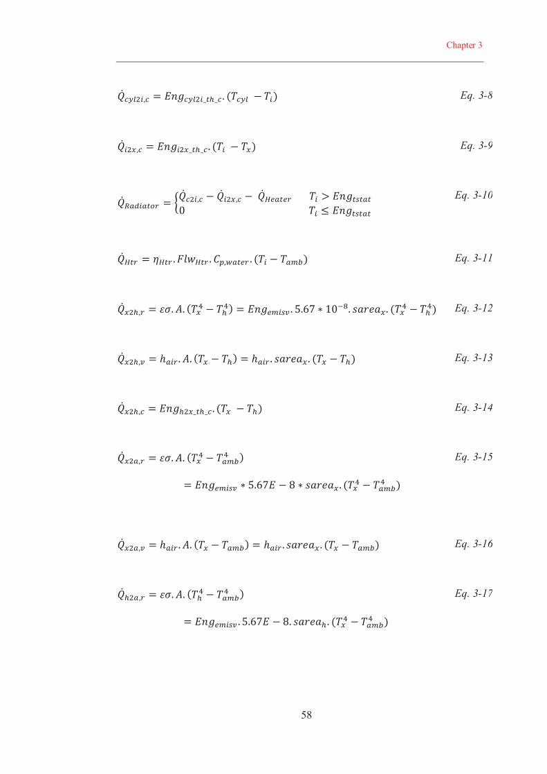
Chapter 3
58
Eq. 3-8
Eq. 3-9
Eq. 3-10
Eq. 3-11
Eq. 3-12
Eq. 3-13
Eq. 3-14
Eq. 3-15
Eq. 3-16
Eq. 3-17

Chapter 3
59
Eq. 3-18
Eq. 3-19
Eq. 3-20
Eq. 3-21
Eq. 3-22
Eq. 3-23
The exhaust mass flow rate, , and temperature, , are also derived from
the lookup tables available from engine dynamometer tests. The exhaust
temperature and mass flow rate, similar to the engine efficiency map, are
tabulated for each engine speed, , and torque, . The accuracy of heat
transfer modelling is quite dependent on how different constants are defined for a
specific engine. Therefore, empirical approaches are employed to accurately fine
tune these constants. In this thesis, the required coefficients are derived from
ADVISOR database.
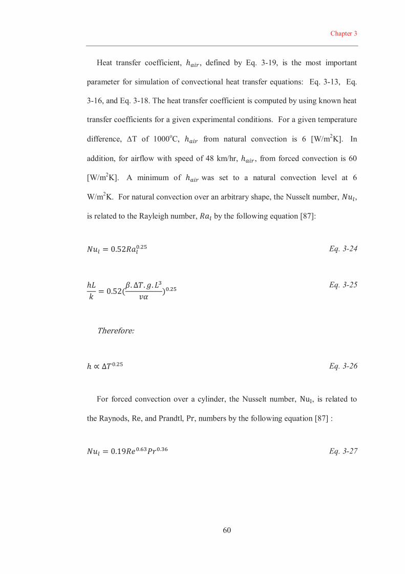
Chapter 3
60
Heat transfer coefficient, , defined by Eq. 3-19, is the most important
parameter for simulation of convectional heat transfer equations: Eq. 3-13, Eq.
3-16, and Eq. 3-18. The heat transfer coefficient is computed by using known heat
transfer coefficients for a given experimental conditions. For a given temperature
difference, T of 1000oC, from natural convection is 6 [W/m2K]. In
addition, for airflow with speed of 48 km/hr, , from forced convection is 60
[W/m2K]. A minimum of was set to a natural convection level at 6
W/m2K. For natural convection over an arbitrary shape, the Nusselt number, ,
is related to the Rayleigh number, by the following equation [87]:
Eq. 3-24
Eq. 3-25
Eq. 3-26
For forced convection over a cylinder, the Nusselt number, , is related to
the Raynods, , and Prandtl, , numbers by the following equation [87] :
Eq. 3-27
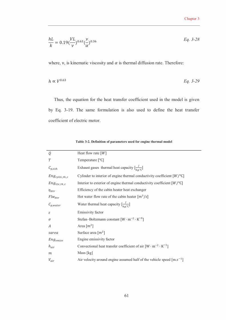
Chapter 3
61
Eq. 3-28
where, , is kinematic viscosity and is thermal diffusion rate. Therefore:
Eq. 3-29
Thus, the equation for the heat transfer coefficient used in the model is given
by Eq. 3-19. The same formulation is also used to define the heat transfer
coefficient of electric motor.
Table 3-2. Definition of parameters used for engine thermal model
Heat flow rate
Temperature
Exhaust gases thermal heat capacity
Cylinder to interior of engine thermal conductivity coefficient
Interior to exterior of engine thermal conductivity coefficient
Efficiency of the cabin heater heat exchanger
Hot water flow rate of the cabin heater
Water thermal heat capacity
Emissivity factor
Stefan–Boltzmann constant
Area
Surface area
Engine emissivity factor
Convectional heat transfer coefficient of air
Mass [kg]
Air velocity around engine assumed half of the vehicle speed [m.
Chapter 3
62
3.6.3 Battery model
The battery model accepts a power request, usually from the power bus, and
returns the available/actual power output of the battery, the battery voltage and
current, and the battery State of Charge (SOC). The battery is modelled with an
equivalent circuit with a perfect open circuit voltage in series with a resistor (see
Figure 1.5). The battery open circuit voltage is a function of the SOC and the
temperature of the battery. The battery resistance is a function of temperature,
charge, and direction of current in charging/discharging modes. The dependency
relationships could be devised empirically in battery test facilities. In this
research, the data from a 6 Ah SAFT Li-ion battery is used from within the
ADVISOR library (see Table 3-1).
The amount of charge that battery can store is considered to be constant, and
the battery voltage exposure is subject to a minimum voltage limit. The
coulombic efficiency of the battery, which is also a function of temperature,
defines the amount of charge that is required to replenish the battery after
discharge. Charging of the battery is limited by a maximum battery voltage limit.
The characteristics of the battery which consists of 10 parallel modules of 25
serial SAFT battery cells are shown in Figure 3.6. The enormous instantaneous
power capability of the battery shows the sizing of the battery is mainly affected
by the energy capacity of the battery rather than its power capacity. The energy
capacity of the battery is designed to let the vehicle cover 64 km of all electric
range when depleting from 90% to 35% SOC (similar to the GM volt 65% SOC
swing window) over the repeated UDDS drive-cycle. The number of parallel
modules also significantly reduces the internal resistance of the battery which

Chapter 3
63
increases the efficiency of the battery accordingly. As the maximum power of the
electric motor is 124 kW, and the battery nominal voltage is 267 V, it is
practically impossible to increase the battery current roughly over 500 A. Hence,
the efficiency of the battery never goes lower than 90%.
As described above, the battery model calculates the battery SOC in response
to the requirements of the power bus. The power loss is computed as losses
plus losses due to Coulombic efficiency. The Coulombic efficiency of the battery
is 96.8%, 99%, and 99.2% for 0˚C, 20˚C, and 41̊C, respectively. The coulombic
efficiency can be calculated for other temperatures by using interpolation.
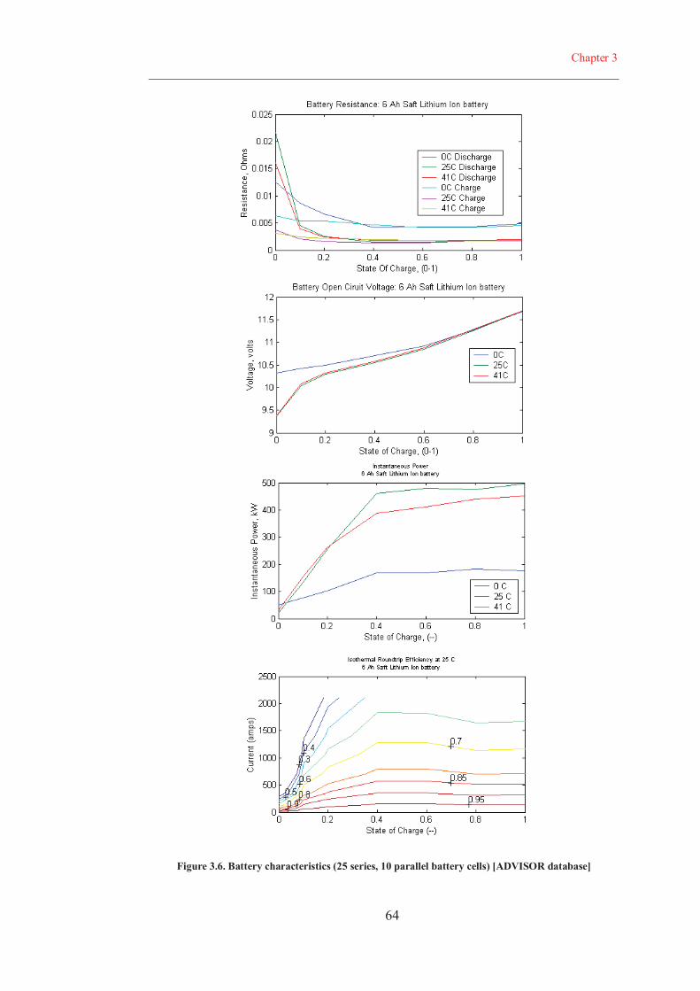
Chapter 3
64
Figure 3.6. Battery characteristics (25 series, 10 parallel battery cells) [ADVISOR database]
Chapter 3
65
Current calculation
Calculation of current is required for each power demand from the battery to
update the charge of the battery in each simulation time-step. The output/input
power of the battery are:
Eq. 3-30
By using Kirchhoff's voltage law:
Eq. 3-31
Using Eq. 3-30 and Eq. 3-31 :
Eq. 3-32
The power is assumed positive when the battery discharges power to the
drivetrain. Rewriting Eq. 3-32, a quadratic equation is derived for the battery
current based on known parameters:
Eq. 3-33
There are two solutions to find the current for this equation, but the larger
solution is not considered because it would require larger current, and thus a lower
terminal voltage, to produce the same power.
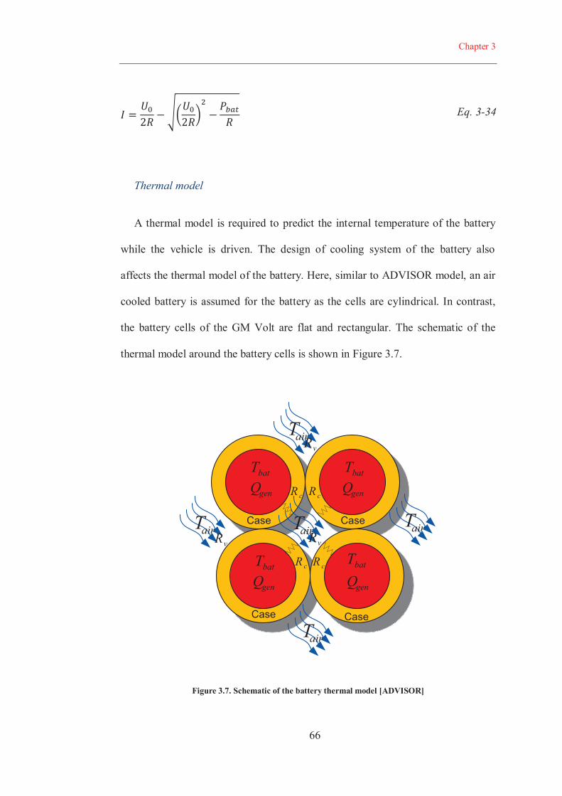
Chapter 3
66
Eq. 3-34
Thermal model
A thermal model is required to predict the internal temperature of the battery
while the vehicle is driven. The design of cooling system of the battery also
affects the thermal model of the battery. Here, similar to ADVISOR model, an air
cooled battery is assumed for the battery as the cells are cylindrical. In contrast,
the battery cells of the GM Volt are flat and rectangular. The schematic of the
thermal model around the battery cells is shown in Figure 3.7.
batT batT
batT batT
airT
genQ genQ
genQ genQ
airT
airT airT
airT
cR
cRcR
cR
vR
vR
vR
Case Case
Case Case
Figure 3.7. Schematic of the battery thermal model [ADVISOR]
Chapter 3
67
The effective thermal resistance is calculated from two parts of conductive
resistance, , and convectional resistance, .
Eq. 3-35
Eq. 3-36
where
Eq. 3-37
Therefore, the heat flow rate to the case of the battery is:
Eq. 3-38
Then the battery core temperature, which is necessary to define internal
resistance, open circuit voltage, and columbic efficiency of the battery can be
derived from Eq. 3-39:
Eq. 3-39
The thermal model of the battery is also required to check the effect of EMS on
its core temperature which accounts for battery aging.
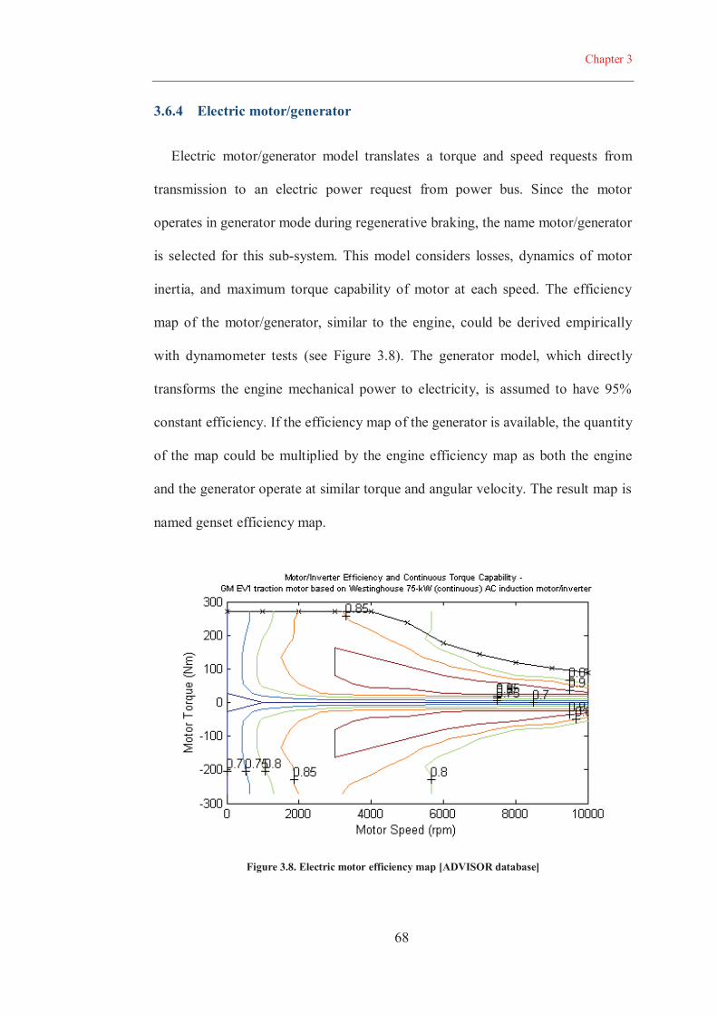
Chapter 3
68
3.6.4 Electric motor/generator
Electric motor/generator model translates a torque and speed requests from
transmission to an electric power request from power bus. Since the motor
operates in generator mode during regenerative braking, the name motor/generator
is selected for this sub-system. This model considers losses, dynamics of motor
inertia, and maximum torque capability of motor at each speed. The efficiency
map of the motor/generator, similar to the engine, could be derived empirically
with dynamometer tests (see Figure 3.8). The generator model, which directly
transforms the engine mechanical power to electricity, is assumed to have 95%
constant efficiency. If the efficiency map of the generator is available, the quantity
of the map could be multiplied by the engine efficiency map as both the engine
and the generator operate at similar torque and angular velocity. The result map is
named genset efficiency map.
Figure 3.8. Electric motor efficiency map [ADVISOR database]
Chapter 3
69
The electric motor power request from the power bus can be calculated with
Eq. 3-40:
Eq. 3-40
In a backward approach, the motor torque, , and speed, , are inputs of the
model to define the required power from the power bus. In the power bus, the
scalar summation of motor and accessories power demand and power available
from the generator is requested from the battery model.
3.6.5 Transmission and final drive
Generally, the role of transmission is more important for conventional or
parallel hybrid electric vehicles. For the series powertrain, a single ratio
transmission is employed to transfer the electric motor torque to the final drive
and wheels. The effects of inertia and gear surface losses could also be considered
in the model. These effects are also modelled empirically via lookup tables that
are mapped for each input torque and speed. In this model, gearbox ratio is 6.67
and the effect of losses is neglected.
3.6.6 Wheel and axel
The wheel and axel model transmits torque and angular velocity requested by
the vehicle model to the final drive model. Friction wastes in the bearing and
inertia of the wheel and axel are also considered in the model. Tyre slip model
defined with lookup-tables based on maximum tractive force that tyres can
Chapter 3
70
transform. The acceleration and deceleration rates defined in drive-cycle modelled
in this research are limited. Therefore, slip never happens in our research
simulations.
3.6.7 Vehicle model
The vehicle model calculates the resistive forces along the longitudinal
direction, rolling, drag, and grading resistances respectively. The
tractive force is calculated using Eq. 3-1. The average speed of the beginning and
the end of each time step is used for the calculations.
Rolling resistance
Rolling resistance is a function of rolling resistance coefficient, , the
normal load of the wheel, , and the road slope, α .
Eq. 3-41
The surface condition of the road also affects the rolling resistance coefficient.
Here,
Eq. 3-42
Road grade
The road grade force is simply calculated with the following equation:
Chapter 3
71
Aerodynamic load
The effect of both aerodynamic load components, shape drag and skin friction,
is formulated into a single drag coefficient, . The drag coefficient could be
found empirically in wind tunnels for each vehicle. The drag force, , is related
to air density, , and vehicle velocity, V:
Acceleration load
The acceleration load is calculated from the following equation:
where, , is the duration of time step and, and , are speeds at the end and
beginning of the time-step, respectively.
Chapter 3
72
3.7 CONCLUSION
In this chapter, different modelling and simulation approaches available in the
literature were introduced. The modelling method selected for this research was
also outlined and different vehicle components model are discussed. Two
different modelling approaches: (i) backward quasi-static and (ii) dynamic
approach based on the theory of dynamic programming are selected to simulate
the performance and efficiency of the vehicle. Specifically, the effect of
temperature on the performance of the engine is modelled as a cold-factor penalty.
This helps simulate the effect of temperature noise factor on the efficiency of
PHEV. The second dynamic modelling approach would be discussed in details in
Chapter 6. The vehicle components are sized to simulate an EREV with 64 km
AER capability.
73
CHAPTER 4
NOISE-FACTORS AND POWER-CYCLE PREDICTION
4.1 INTRODUCTION
Since the knowledge of driving scenario as a priori has been proven essential
for the globally optimal energy management approaches, drive-cycle simulations
have been carried out in several existing works. Especially, for the PHEV blended
mode energy management strategies, the knowledge of driving scenario helps the
charge management of the battery during the journey. The knowledge of travel
Chapter 4
74
distance or preferably drive-cycle would change the way the stored electric energy
in the battery is allocated during the journey to optimise the fuel consumption.
Gao et al. suggested a manual shifting mode between the EV and CS modes to
somehow affect the knowledge of future driving pattern [13]. That is, the driver
can shift to the EV mode for low speed in congested city driving and return back
to the CS or a moderate CD modes for high speed in highway driving. Having the
journey distance information, Sharer et al. calibrated engine-ignition power
thresholds for different journey distances and concluded that the basic information
on trip distance can decrease the fuel consumption [38]. Gong et al. suggested that
it is possible to improve the control strategy of PHEV and implement a
deterministic DP EMS, if the trip information is determined as a priori by means
of recent advancements in intelligent transportation system (ITS) based on the use
of global positioning system (GPS) and geographical information system (GIS)
[49]. A model predictive control approach was used in test vehicles equipped with
telemetric system [88, 89]. The controller of a HEV calibrates the ratio of the
charge/discharge of the battery by means of the traffic information and road grade
in a method suggested by Deguchi [90].
This chapter introduces an applicable solution to predict the driving scenario
before the journey starts. Additionally, the noise factors affecting the power
demand of the vehicle are categorised. A comprehensive knowledge of the noise
factors guarantees accurate prediction of the driving pattern.
Chapter 4
75
4.2 POWER-CYCLE AND NOISE FACTORS
As explained above, development of the optimal EMSs requires power-cycle
information in advance, especially for the charge management of PHEVs in a
blended mode operation. However, the drive-cycles are inadequate to predict the
realistic power demand of the vehicle. The reason is that apart from the vehicle
velocity profile, several other noise factors can affect the vehicle power demand.
Therefore, a control strategy only based on the drive-cycle cannot provide a
correct solution and might even deteriorate the performance of the vehicle. The
benefit of having a large battery on-board could be sacrificed by reaching the
destination with surplus electric energy. That is, a blended mode EMS could
deteriorate the performance of a PHEV when compared with a simple AER-CS, if
defined based on an inaccurate driving scenario prediction. Consequently, it is
necessary to accurately define a power-cycle that can predict the vehicle required
power consisting of both the traction and accessories power demand.
Noise factors affecting the power demand and performance of different
components of a PHEV, as well as the velocity trajectory need to be taken into
account to predict a realistic power trajectory. These noise factors consist of (i)
traffic diversity and aggressive driving, (ii) road grade, (iii) wind, (iv) battery
aging, and (v) ambient temperature. These noise factors can significantly alter the
power demand even in identical journeys and drive-cycles. Besides, the
performance of the vehicle components might be altered in different ambient
temperatures and by aging. Especially with aging of the vehicle, the battery
degradation reduces the available electric energy on-board of a PHEV. These
noise factors are non-negligible parameters which have been completely neglected
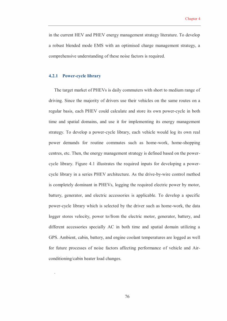
Chapter 4
76
in the current HEV and PHEV energy management strategy literature. To develop
a robust blended mode EMS with an optimised charge management strategy, a
comprehensive understanding of these noise factors is required.
4.2.1 Power-cycle library
The target market of PHEVs is daily commuters with short to medium range of
driving. Since the majority of drivers use their vehicles on the same routes on a
regular basis, each PHEV could calculate and store its own power-cycle in both
time and spatial domains, and use it for implementing its energy management
strategy. To develop a power-cycle library, each vehicle would log its own real
power demands for routine commutes such as home-work, home-shopping
centres, etc. Then, the energy management strategy is defined based on the power-
cycle library. Figure 4.1 illustrates the required inputs for developing a power-
cycle library in a series PHEV architecture. As the drive-by-wire control method
is completely dominant in PHEVs, logging the required electric power by motor,
battery, generator, and electric accessories is applicable. To develop a specific
power-cycle library which is selected by the driver such as home-work, the data
logger stores velocity, power to/from the electric motor, generator, battery, and
different accessories specially AC in both time and spatial domain utilizing a
GPS. Ambient, cabin, battery, and engine coolant temperatures are logged as well
for future processes of noise factors affecting performance of vehicle and Air-
conditioning/cabin heater load changes.
.
Chapter 4
77
Power to/from Motor
Power to/from Battery
Driver Route Selection
Cabin/Engine temperature
GPS
Time
Power CycleLibrary
Power CyclePrediction
SoC
Auxiliary Power
Series Powertrain Similar to GM Volt
Temperature and Humidity
Figure 4.1. Required inputs for developing the power-cycle library
PHEVs employ an in-built control strategy defined by OEM, normally an
AER-CS similar to what has been designed for GM Volt. However, for the known
power-cycles, which would be defined later on by each vehicle owner, a more
sophisticated energy management strategy would be implemented. The power
demand information can be repeatedly stored in the low cost memory devices and
updated whenever necessary to account for stochastic factors over time. The
logged power-cycle based on the real commute history can be used to reasonably
predict many stochastic factors. Still, good understanding of the noise factors is
essential to predict a realistic power-cycle based on the vehicle power-cycle
library and update it on-line even during the journey.
Chapter 4
78
4.2.2 Noise factors
The noise factors can potentially modify the power demand and alter the
performance of a PHEV. The proposed power-cycle library method that could
help in the prediction of the noise factors is explained in the following.
Effect of traffic diversity and aggressiveness factor on velocity
According to Eq. 3-2, vehicle velocity is the most important factor for
prediction of different traction power components. One of the major advantages of
power-cycle library over the drive-cycle prediction methods is that the prediction
of velocity is more accurate considering driver behaviour and various road traffic
conditions in a specific journey. In particular, for daily commutes such as home-
work which mostly occur during the rush hours, the drive-cycle modelling based
on maximum speed limits, employed in references [49, 91], would be far from
reality. The chance of stopping when the vehicle reaches traffic lights also alters
the power-cycle during deceleration and acceleration or by the accessories’ power
demand during stop time.
The power-cycle library inherently considers the aggressiveness factor of
different drivers that affect the power demand during accelerating or braking. This
means that the power-cycle library could save driver’s name and define an
aggressiveness factor for each driver. The term in Eq. 3-2 is the
power required for acceleration or braking.
Chapter 4
79
Road grade
The road grade considerably alters the power demand of the vehicle. In
reciprocal journeys, any downhill part would be uphill in return. Correct
allocation of electric energy for downhill or uphill parts of the journey would
improve the efficiency and the battery health in mountainous areas. By means of
using a GPS which provides elevation information, it is possible to predict road
grade power for a journey in advance.
Wind
The crosswind speed against the vehicle movement raises the power demand of
the vehicle especially in high speed driving at highways; hence, the drag force
increases with the square of velocity. For instance, the drag force at 100 km/hr is
around 30% higher with 20 km/hr crosswind.
Eq. 4-1 represents the drag force which is a function of both vehicle and wind
speeds, , vehicle frontal area, , drag coefficient, , and air density, .
Based on the daily wind speed and direction forecasts and the journey speed
and direction saved in the power-cycle library, Eq. 4-1 can predict the effect of
daily wind velocity on vehicle power demand.
Chapter 4
80
Temperature and change in aerodynamic force
Even change in air density can cause discrepancy for the power demand
prediction as it changes around 25% between temperatures and .
This change is proportional to the same drag force change according to Eq. 4-1 .
Temperature and engine and catalyst converter operation
It is well known that cold engine operation increases fuel consumption and
pollution of the vehicle [92, 93]. For instance, the hydrocarbon and carbon
monoxide emissions increases by 650% and 800% respectively at ,
compared to the standard certification values at . The low ambient
temperature raises lubricating oil viscosity and thus results in higher mechanical
losses during engine cold start. In addition, combustion is affected due to lower
ignitability of the fuel mixture. The low ambient temperature can also delay the
three-way catalyst (TWC) activation, which is one of the most important reasons
accounted for high emissions at cold start. The full operational temperature of
TWC is around . The research on EURO4 emission compliant vehicle
shows that for similar and even more aggressive than ECE 15 urban driving cycle,
the lubricating oil temperature increases form the ambient temperature of
to the full warmed up value in about 15 minutes, and it takes
100 seconds for upstream and 200 seconds for downstream of TWC to reach
[93]. The issue of cold start and warm-up period is even more significant
for HEVs and PHEVs. When the vehicle is controlled by a blended mode charge
management strategy, the engine on/off shifting occurs more frequently, and the
Chapter 4
81
engine cools down when vehicle operates in the EV mode. The all electric range
followed by the charge sustaining mode EMS for EREVs intrinsically solves this
issue as the operation of EREV is similar to that of a HEV during the CS mode.
Cold engine operation, however, should be investigated when dealing with the
blended mode EMS. The cold engine fuel consumption penalty, cold-factor, is
formulated in Section 3.6.2.
Temperature and battery performance
Battery thermal management is the current state of the art in battery designing.
Temperature affects both performance and aging process of the battery. Battery
have minimum operational temperature since their performance is degraded
significantly in low temperatures. A plugged in battery is kept warm enough so
that it can be used immediately. However, if the battery temperature goes below
the minimum operational temperature, the engine should run until the battery
warms up even if the battery is fully charged. On the other hand, high temperature
significantly accelerates the aging and the degrading of battery, and the battery
cooling system causes parasitic loads. From the energy management point of
view, the effect of temperature on battery performance is significant when the
operation is compared for summer or winter extreme temperatures. However, the
power-cycle library based energy management provides the performance
characteristics of battery in the specific time of the year. An important benefit of
the library control approach is the flexibility to define effective energy
management strategy regardless of different environmental and geographic
condition.
Chapter 4
82
Temperature and air-conditioning/cabin heating power demand
Unlike conventional vehicles in which the compressor of the air conditioning
system is connected mechanically to the engine, a separate electric motor propels
the compressor in PHEVs and most of HEVs. The AC can be considered as the
most significant auxiliary load in a vehicle. As an example, the power demand of
the AC compressor is equivalent to the vehicle when driving steadily at 56 kph
[31]. The fuel economy of a vehicle drops substantially when the AC compressor
load is added. This effect is even larger for high fuel economy vehicles. AER
would be considerably reduced in PHEVs since the compressor is powered by the
battery. A 3 kW accessory load will decrease AER on a repeated EPA Urban
Dynamometer Driving Schedule (UDDS) by 38% [94]. During hot soaking which
means parking in the open on a sunny and warm day, the interior temperature
could easily exceeds 70°C. Through the initial surge cooling interval, the
compressor of compact and mid-sized vehicles consumes around 2.9 kW to 3.4
kW respectively [95]. However, to avoid initial surge if the PHEV is connected to
the grid, it is possible to use external electricity to start the AC or heater system in
appropriate times before the journey starts. This opportunity simultaneously
provides comfort and saves valuable battery energy.
The required power for the cabin heater and safety related demister is another
issue in PHEVs when there is no hot water available from the engine coolant
during the EV mode. It is necessary to devise a parallel electric heating system to
warm up the cabin similar to electric vehicles. Using electric energy for heating is
huge waste in comparison with engine coolant free energy. Heat pumps are not
applicable for automotive heating applications because of the evaporator heat
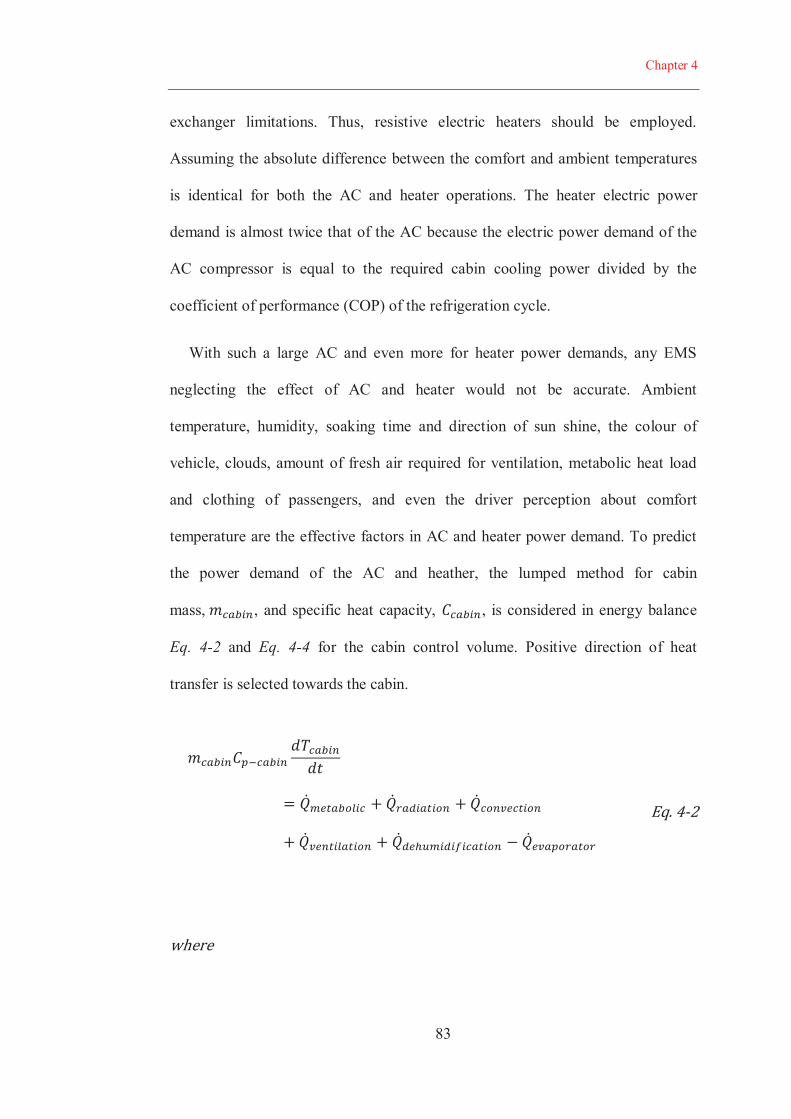
Chapter 4
83
exchanger limitations. Thus, resistive electric heaters should be employed.
Assuming the absolute difference between the comfort and ambient temperatures
is identical for both the AC and heater operations. The heater electric power
demand is almost twice that of the AC because the electric power demand of the
AC compressor is equal to the required cabin cooling power divided by the
coefficient of performance (COP) of the refrigeration cycle.
With such a large AC and even more for heater power demands, any EMS
neglecting the effect of AC and heater would not be accurate. Ambient
temperature, humidity, soaking time and direction of sun shine, the colour of
vehicle, clouds, amount of fresh air required for ventilation, metabolic heat load
and clothing of passengers, and even the driver perception about comfort
temperature are the effective factors in AC and heater power demand. To predict
the power demand of the AC and heather, the lumped method for cabin
mass, , and specific heat capacity, , is considered in energy balance
Eq. 4-2 and Eq. 4-4 for the cabin control volume. Positive direction of heat
transfer is selected towards the cabin.
Chapter 4
84
and
where the passengers’ metabolic heat load, , is affected by the number
of passengers. Solar radiation load, , is related to sun radiation heat
flux, , and the incidence surface, S. For convectional heat transfer, ,
heat transfer coefficient, h, behaviour is very complex and varying regarding
vehicle and wind speed. A is effective area of convection heat transfer. Fresh air
mass flow rate, , causes ventilation heat load, , which is related to
the air specific heat capacity, , consisting both air and its water content [96,
97]. If dehumidification is necessary, the dehumidification load, ,
is related to condensed water mass rate, , water latent heat vaporization,
, and water specific heat capacity, . COP is coefficient of performance of
Chapter 4
85
the AC. Eq. 4-2 can be simplified to Eq. 4-4 when a warming function is
required.
Prediction of all the parameters that can affect the AC power demand in a
drive-cycle is complex, particularly when the passenger perception plays an
important role. The power-cycle library could capture the general trend of the AC
or heater operation requirements of a specific driver for a specific commute.
Having access to a library of AC power demand for a routine commute, the AC
power demand would be easier to derive based on lookup tables and simpler but
more accurate equations.
For a routine commute, we can assume that for Eq. 4-2 and Eq. 4-4,
remain unchanged, as we can assume that the driver perception about
the comfort temperature is unchanged. Although S, A, h change with the vehicle
speed and the direction of route against the sun, but we can assume these
parameters change in a repeatable manner for a specific journey. For a desired
cabin temperature, to predict the everyday AC power demand, the only remaining
variables are ambient temperature, humidity, and sun radiation heat flux for the
specific day. With a developed library of AC or heater power demand by means
of interpolation methods, the trend of required power demand of the AC or heater
Chapter 4
86
are predictable with enough accuracy as required for the charge management of
PHEVs.
Battery aging
State of health of the battery determines the amount of on-board available
electric energy that PHEV could allocate for a specific power-cycle. The PHEV
battery duty cycle is one of the most aggressive one that battery may encounter
[98]. The battery life is dependent upon both storage and cycling. Capacity
degradation and resistance growth have been shown to be dependent on a number
of operational parameters. The following equation shows how the cycling, and the
storage time affect resistance [99]:
where t is storage time, and is number of cycles. Coefficients
and are a function of the given state of charge swing, ,
battery cell temperature, , and voltage exposure, .
There are two mechanisms described for the capacity fade. Lithium loss is the
dominant mechanism during storage, and isolation of the active sites is dominant
during cycling [99]. Lithium capacity, , and active sites capacities, , are
defined by the following equations. The minimum of them would be the actual
capacity, . are constant values derived from experiments.
Chapter 4
87
The impedance growth and the capacity fade due to the elevated voltage and
temperature are inevitable. For instance, a battery stored in 35°C would have
around 6% higher Lithium capacity loss in comparison to the same battery stored
at 20°C after 5 years [99]. Since a PHEV may be used under different
geographical locations with various climates, and depending on the
aggressiveness of the driving pattern, the state of health of each battery would be
different during the effective life of a PHEV. The EV mode followed by the CS
mode EMS would not be affected by this noise factor. The only difference that the
driver would notice is that the shift from the EV to CS modes occurs earlier
compared to an ordinary vehicle for identical journeys. However, for the blended
mode EMS, the real available battery energy is one of the initial input data for the
controller. The power-cycle library could save the available energy of battery each
time it is used. As a result, the slow dynamics of the battery aging is intrinsically
considered inside the controller based on the power-cycle libraries.
4.3 CONCLUSION
The blended mode energy management strategies are efficient choices for
energy management of plug-in hybrid electric vehicles (PHEVs). Development of

Chapter 4
88
an optimal energy management strategy including an appropriate battery charge
management requires the knowledge of the vehicle power demand trajectory in
advance. Other than the speed-time profile, i.e. drive-cycle, there are many noise
factors which affect both the drivetrain power demand and the vehicle
performance. Therefore, the term power-cycle was defined in this chapter. In
addition, the noise factors that could potentially alter the power demand of the
vehicle even in identical journeys were discussed. These noise factors consist of
driver aggressiveness factor, traffic, road grade and environmental conditions like
temperature, humidity, wind, and sun radiation heat flux.
Due to the nature of noise factors, power-cycle prediction and their interaction
with the performance of the vehicle, the effect of these factors for each PHEV
should be investigated individually. The power-cycle library concept proposed in
this chapter helps achieve more accurate power-cycle prediction for repetitive
commutes of PHEVs owners. The library of power-cycles provides a basic
knowledge of power trajectory in both time and spatial domains. This helps
prediction of the velocity and grade trajectory of any selected route with
acceptable precision. Then, it is necessary to update the power-cycle before each
journey for changes accounted for environmental disturbances like temperature,
humidity, sun radiation, and wind.
89
CHAPTER 5
ENERGY MANAGEMENT OF PHEVS: A RULE-BASED APPROACH
5.1 INTRODUCTION
It has been demonstrated that the blended mode or the controlled charge
management strategies are efficient choices for energy management of plug-in
hybrid electric vehicles [13, 36-39]. In this chapter, a rule-based EMS is
introduced to demonstrate the benefits of having access to the proposed power-
cycle library described in Chapter 4. The EMS also considers the effect of the
temperature noise factor on engine cold-factor penalty. The model of a series
EREV capable of 64 km AER, described in Chapter 3, is employed to investigate
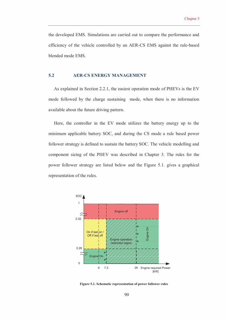
Chapter 5
90
the developed EMS. Simulations are carried out to compare the performance and
efficiency of the vehicle controlled by an AER-CS EMS against the rule-based
blended mode EMS.
5.2 AER-CS ENERGY MANAGEMENT
As explained in Section 2.2.1, the easiest operation mode of PHEVs is the EV
mode followed by the charge sustaining mode, when there is no information
available about the future driving pattern.
Here, the controller in the EV mode utilizes the battery energy up to the
minimum applicable battery SOC, and during the CS mode a rule based power
follower strategy is defined to sustain the battery SOC. The vehicle modelling and
component sizing of the PHEV was described in Chapter 3. The rules for the
power follower strategy are listed below and the Figure 5.1. gives a graphical
representation of the rules.
Engine off
On if last on /Off if last off
Eng
ine
On
Engine On
Engine operationrestricted region
n
SOC
1
0.32
0.28
0Engine required Power
[kW]6 267.2
Figure 5.1. Schematic representation of power follower rules
Chapter 5
91
The rules employed for this controller are:
Engine is kept off until the battery charge reaches minimum applicable
SOC (AER rule).
Engine may be turned off if the battery SOC reaches the defined high
limit (here 32%).
Engine may be turned on again if the power required by the vehicle gets
high enough (here 7.2 kW).
Engine may be turned off again if the power required by the vehicle gets
low enough (here 6 kW).
Engine may be turned on if the battery SOC gets to a defined low limit
(here 28%).
When the engine is on, its power output tends to follow the power
required by the vehicle, accounting for the losses in the generator so that
the generator power output matches the vehicle power requirement. As
the wheel and engine speeds are independent, the engine torque and
speed are selected based on the designed curve or confined optimal
operation line (see Section 5.2.1).
The engine output power may be adjusted by the SOC bringing the SOC
back to the centre of its operating range.
The engine output power may be kept above a minimum value (here 6
kW).
The engine output power may be kept below a maximum value (which is
enforced unless the SOC gets too low) (here 26 kW).
Chapter 5
92
The engine output power may be allowed to change no faster than a
prescribed rate (+2 and -3 kW/s).
If engine turns on, it is kept on for at least a prescribed time,
(here 60 s).
During engine-on, the battery only provides the power shortage required by the
vehicle when the engine inertia or the power follower rate limiter rules cause a
difference between the powertrain required power and the engine available power.
Also, when very high power demand (more than 26 kW) is required, the battery
compensates the power deficit. The battery SOC range between 0.28 to 0.32,
defined in the Figure 5.1, are adequate for the vehicle operation like a
conventional HEV when the battery is depleted to minimum SOC of 0.3. The
engine power output range between 6 kW to 26 kW is defined as if the engine
efficiency is constrained into the 0.3 contour depicted in the engine efficiency
map of Figure 3.4. The 1.2 kW difference between, 6 kW and 7.2 kW, vehicle
power demand thresholds to switch the engine on/off, engine power change rate
limiter, and minimum engine on time are defined to prevent unsteady and
transient operation of the engine.
5.2.1 Confined optimal operation line
The engine-generator operation is independent of the vehicle speed in the
series architecture. Therefore, the engine-generator can operate over its optimal
operation point for any required power. The combination of these optimal
operation points defines a line in the engine-generator brake specific fuel
consumption (BSFC) map called confined optimal operation line (COOL). (see
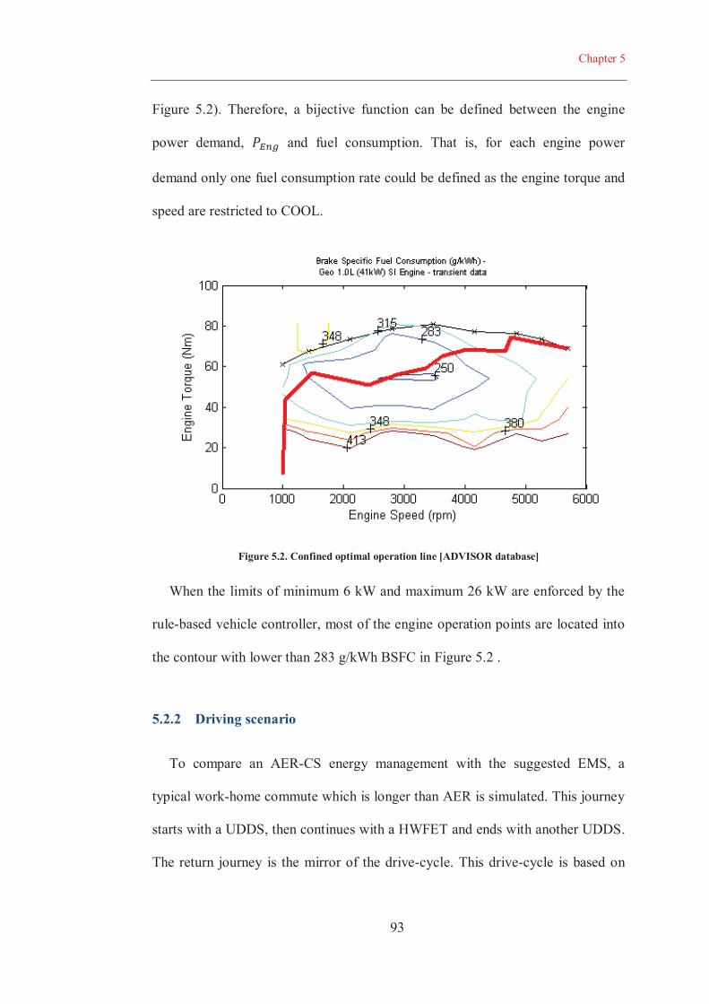
Chapter 5
93
Figure 5.2). Therefore, a bijective function can be defined between the engine
power demand, and fuel consumption. That is, for each engine power
demand only one fuel consumption rate could be defined as the engine torque and
speed are restricted to COOL.
Figure 5.2. Confined optimal operation line [ADVISOR database]
When the limits of minimum 6 kW and maximum 26 kW are enforced by the
rule-based vehicle controller, most of the engine operation points are located into
the contour with lower than 283 g/kWh BSFC in Figure 5.2 .
5.2.2 Driving scenario
To compare an AER-CS energy management with the suggested EMS, a
typical work-home commute which is longer than AER is simulated. This journey
starts with a UDDS, then continues with a HWFET and ends with another UDDS.
The return journey is the mirror of the drive-cycle. This drive-cycle is based on
Chapter 5
94
the idea that the driver starts the car in a suburban area and after driving on a
highway arrives to a downtown urban area where the destination elevation is
around 400 meters higher than the start point. Then, the vehicle returns back to
complete the 80 km journey. Figure 5.6 (a) shows the speed and elevation of the
vehicle in the defined cycle. The power-cycle in Figure 5.6 (b) consists of both
traction and accessories such as air conditioner power demand.
5.3 PROPOSED RULE BASED BLENDED MODE EMS
The difference between the total energy demand in the power-cycle and the
available battery energy is equal to the required energy from the engine/generator
or the energy share provided by fuel. The series drivetrain has the advantage of
blending both the battery and the engine power independent of the powertrain
required load and the vehicle speed. It is possible to use the engine as a power
source anywhere in a journey to provide its share in total energy demand of a
power-cycle. However, the amount of engine energy share should be anticipated
in advance by means of the power-cycle prediction method described in Chapter
4. Fuel consumption in the series PHEV architecture with an AER-CS strategy
only depends on the engine/generator performance during the end of power-cycle
when the vehicle operates in the CS mode. With the knowledge of the power-
cycle, it is possible to find efficient sections to get the engine energy share. These
sections should be long enough to prevent complications associated with the
transient operation. In the following, a three-step procedure to define a controlled
charge management strategy is described. This procedure considers the engine
temperature as one of the most important noise factors on the engine performance.
Chapter 5
95
Intentionally, to have a fair comparison between the AER-CS and the proposed
blended mode energy management, the power follower strategy for the vehicle
controller, and also the regenerative braking rules are kept unchanged. The only
difference is more efficient charge management that is defined with the proposed
EMS compared to the AER-CS.
The suggested EMS is developed in a three steps (i) step 1: Hot engine
efficiency cycle, CD1 strategy, (ii) step 2: Engine warmth conservation, CD2
strategy and (iii) step 3: Engine cold start investigation, CD3 strategy (see Figure
5.3). Since a deterministic approach is chosen for the rule-based EMS, the first
perquisite to implement the method is the knowledge of the power-cycle and
available charge in the battery. In the first step, it is assumed that temperature
noise factor does not affect the performance of the vehicle. As a result, the hot
engine efficiency map is used to develop the charge management strategy. In the
second step, however, the engine thermal model is employed to explore the effect
of the temperature noise factor. Finally, the last step investigates the possibility of
elimination of excessive cold start-warm up in the reciprocal commutes if it
secures more efficient operation of the vehicle.
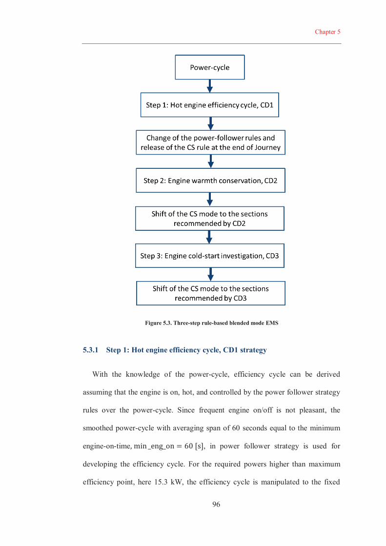
Chapter 5
96
Figure 5.3. Three-step rule-based blended mode EMS
5.3.1 Step 1: Hot engine efficiency cycle, CD1 strategy
With the knowledge of the power-cycle, efficiency cycle can be derived
assuming that the engine is on, hot, and controlled by the power follower strategy
rules over the power-cycle. Since frequent engine on/off is not pleasant, the
smoothed power-cycle with averaging span of 60 seconds equal to the minimum
engine-on-time , in power follower strategy is used for
developing the efficiency cycle. For the required powers higher than maximum
efficiency point, here 15.3 kW, the efficiency cycle is manipulated to the fixed
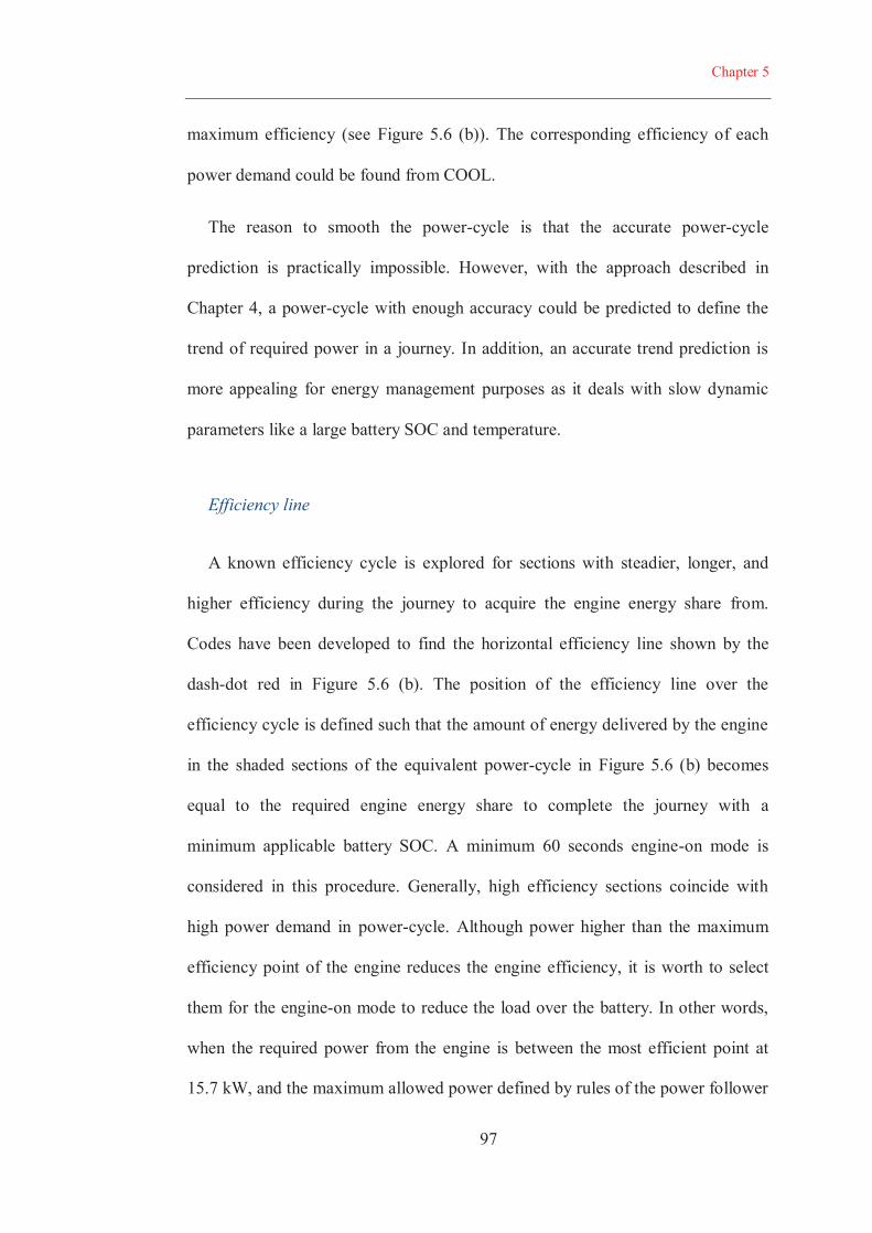
Chapter 5
97
maximum efficiency (see Figure 5.6 (b)). The corresponding efficiency of each
power demand could be found from COOL.
The reason to smooth the power-cycle is that the accurate power-cycle
prediction is practically impossible. However, with the approach described in
Chapter 4, a power-cycle with enough accuracy could be predicted to define the
trend of required power in a journey. In addition, an accurate trend prediction is
more appealing for energy management purposes as it deals with slow dynamic
parameters like a large battery SOC and temperature.
Efficiency line
A known efficiency cycle is explored for sections with steadier, longer, and
higher efficiency during the journey to acquire the engine energy share from.
Codes have been developed to find the horizontal efficiency line shown by the
dash-dot red in Figure 5.6 (b). The position of the efficiency line over the
efficiency cycle is defined such that the amount of energy delivered by the engine
in the shaded sections of the equivalent power-cycle in Figure 5.6 (b) becomes
equal to the required engine energy share to complete the journey with a
minimum applicable battery SOC. A minimum 60 seconds engine-on mode is
considered in this procedure. Generally, high efficiency sections coincide with
high power demand in power-cycle. Although power higher than the maximum
efficiency point of the engine reduces the engine efficiency, it is worth to select
them for the engine-on mode to reduce the load over the battery. In other words,
when the required power from the engine is between the most efficient point at
15.7 kW, and the maximum allowed power defined by rules of the power follower

Chapter 5
98
controller at 26 kW, logically these sections are acceptable for the engine
operation. The shift of the engine operation from the end (CS mode) to the high
power demand sections of the journey reduces the maximum power required from
the battery that is beneficial for its state of health. The first step is named Charge
Depleting 1 (CD1). The schematic illustration of the step one is depicted in Figure
5.4 and the flowchart of the finding the efficacy line is given in Figure 5.5.
The CD1 over the defined power-cycle mostly selects the first section of the
journey for the engine operation while the drive-cycle is similar in both go and
return journeys. The reason is the slope of the road which significantly increases
the power demand of the vehicle (see Figure 5.6 (b)). Logically, the engine energy
share is allocated in high speed sections of each side of the cycle. There is one
section, around t=4900, where the efficiency is higher than the efficiency line but
is not selected for the engine operation. The reason is that the section is shorter
than minimum engine on time threshold, 60 sec.
When the engine-on sections are defined with CD1, to implement it in the
vehicle controller, the rules of power follower are manipulated. The rule “Engine
is kept off until the battery charge reaches minimum applicable SOC (AER rule)
is eliminated, as this rule enforces the AER-CS EMS for the PHEV. The rules
which enforce charge sustaining at minimum applicable SOC are also
manipulated to keep the battery SOC constant during the engine-on sections
( , , …) defined by CD1. Therefore, the vehicle operation in the CS
mode moves to the engine-on sections instead of concentrating at the end of
journey.
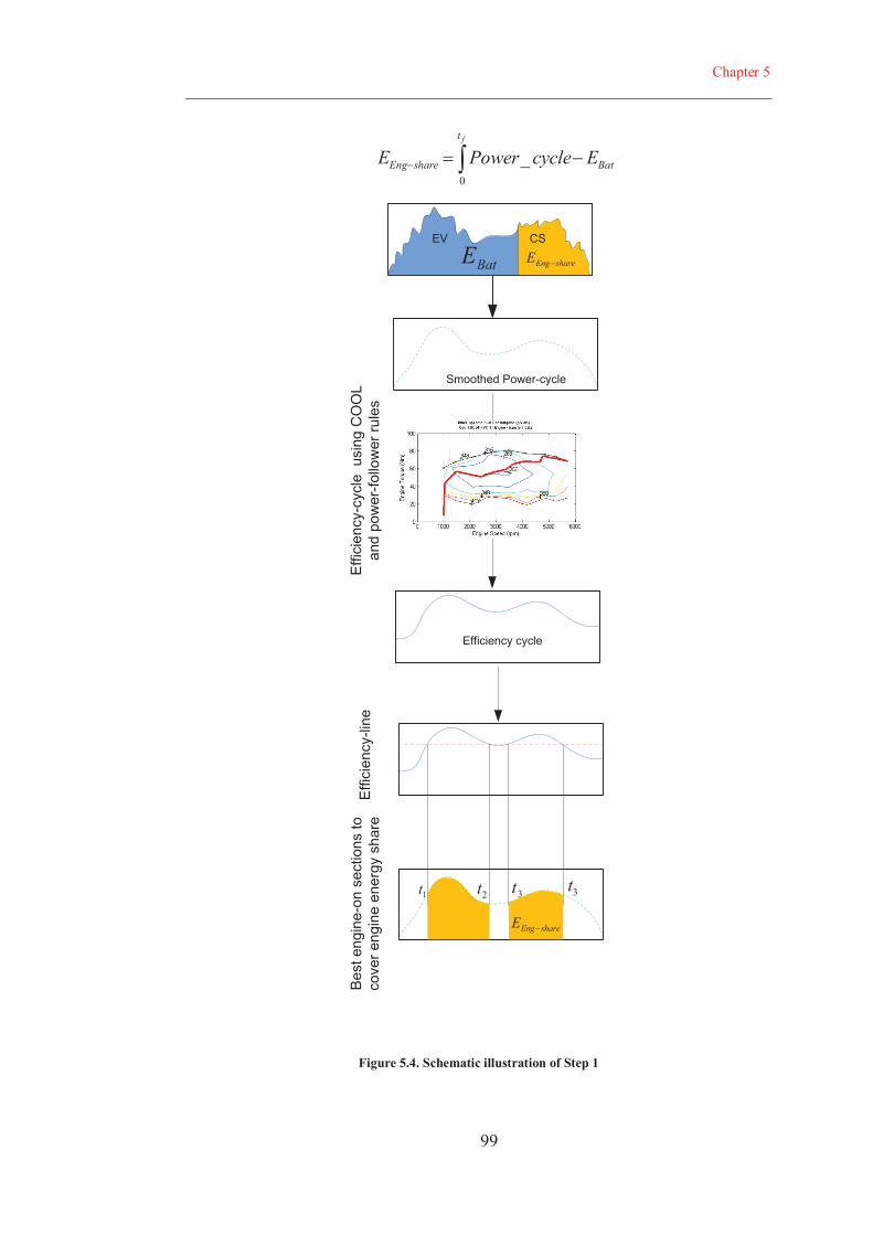
Chapter 5
99
Bat
t
shareEng EcyclePowerEf
0
_
EV
shareEngECS
BatE
Effi
cien
cy-c
ycle
usin
gC
OO
Lan
dpo
wer
-follo
wer
rule
sSmoothed Power-cycle
Efficiency cycle
shareEngE
1t 3t2t 3t
Effi
cien
cy-li
neB
est e
ngin
e-on
sect
ions
toco
ver e
ngin
een
ergy
shar
e
Figure 5.4. Schematic illustration of Step 1
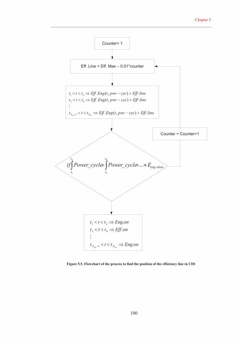
Chapter 5
100
Eff. Line = Eff. Max – 0.01*counter
Counter= 1
shareeng
t
t
t
t
EcyclePowercyclePowerif ...__4
3
2
1
lineEffcycpwrtEngEffttt
lineEffcycpwrtEngEfftttlineEffcycpwrtEngEffttt
onon NN .),(.
.),(..),(.
1
43
21
onEngttt
onEfftttonEngttt
onon NN .
..
1
43
21
Counter = Counter+1
Figure 5.5. Flowchart of the process to find the position of the efficiency line in CD1
Chapter 5
101
5.3.2 Step 2: Engine warmth conservation, CD2 strategy
Since the efficiency cycle in Step 1 is formulated based on the hot engine
efficiency map, it does not consider the effect of temperature on the engine
performance. Cold engine operation during the shifting between the EV and the
engine-on modes at CD1 is a point of concern. The engine thermal model is a
prerequisite to determine the effect of the cold engine operation. The engine
thermal model, described in Section 3.6.2, is employed to investigate the effect of
temperature on the engine performance.
The first question that needs to be answered when considering the effect of the
engine temperature on the performance is to investigate whether it is more
efficient to select the engine-on sections only based on the hot engine efficiency
cycle, or to choose these sections more concentrated to conserve the engine
warmth. To answer this question, the longest engine-on sections selected in CD1
are chosen in each side of the go and return journeys as there is a cool-down
period at the middle of the journey. The nearby sections with less than 60 seconds
engine-off interval are also added to the two longest sections at each side. It is
obvious that these longest sections would be selected for engine operation even
when the engine temperature noise factor comes to account. In other words, the
engine-on sections might concentrate around the longest sections if it is more
efficient to run the engine in lower efficiency cycle region (derived from hot
engine assumption) but in higher temperatures. It is assumed that temperature is
constant and equal to the thermostat set temperature during the chosen sections.
That is, the cold-factor from Eq. 3-6 for the longest section of the engine-on is
one. Applying the engine temperature code, coolant temperature and consequently
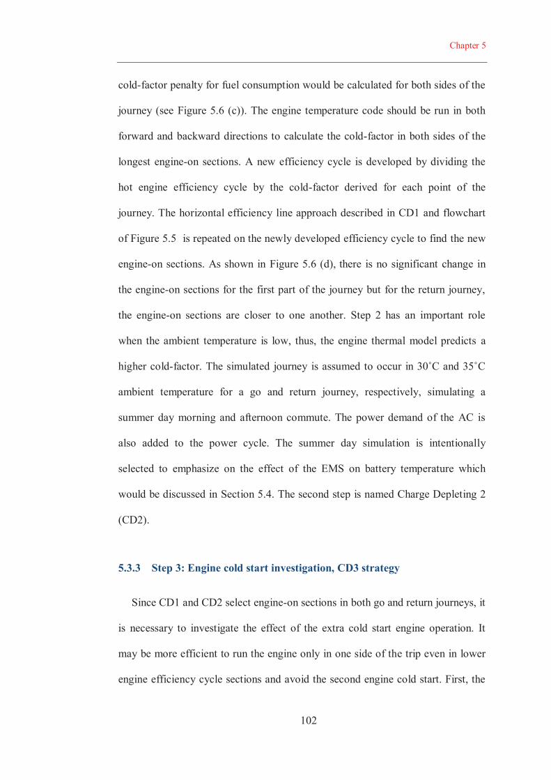
Chapter 5
102
cold-factor penalty for fuel consumption would be calculated for both sides of the
journey (see Figure 5.6 (c)). The engine temperature code should be run in both
forward and backward directions to calculate the cold-factor in both sides of the
longest engine-on sections. A new efficiency cycle is developed by dividing the
hot engine efficiency cycle by the cold-factor derived for each point of the
journey. The horizontal efficiency line approach described in CD1 and flowchart
of Figure 5.5 is repeated on the newly developed efficiency cycle to find the new
engine-on sections. As shown in Figure 5.6 (d), there is no significant change in
the engine-on sections for the first part of the journey but for the return journey,
the engine-on sections are closer to one another. Step 2 has an important role
when the ambient temperature is low, thus, the engine thermal model predicts a
higher cold-factor. The simulated journey is assumed to occur in 30˚C and 35˚C
ambient temperature for a go and return journey, respectively, simulating a
summer day morning and afternoon commute. The power demand of the AC is
also added to the power cycle. The summer day simulation is intentionally
selected to emphasize on the effect of the EMS on battery temperature which
would be discussed in Section 5.4. The second step is named Charge Depleting 2
(CD2).
5.3.3 Step 3: Engine cold start investigation, CD3 strategy
Since CD1 and CD2 select engine-on sections in both go and return journeys, it
is necessary to investigate the effect of the extra cold start engine operation. It
may be more efficient to run the engine only in one side of the trip even in lower
engine efficiency cycle sections and avoid the second engine cold start. First, the

Chapter 5
103
side with the higher engine-on sections from CD2 is selected which logically
provides larger share in the engine energy demand. Similar to the Step 1, the
aforementioned efficiency line procedure is repeated to cover all the engine
energy demand from only one side of the journey assuming that the vehicle
operates in the EV mode for the return journey. The hot engine operation
efficiency of the newly added sections, with darker colour in Figure 5.6 (e), is
compared with the other side CD2 engine efficiency while the cold-factor penalty
is considered. It is assumed that the efficiency of the newly added sections is
equal to that of the hot engine because at least one cold start is inevitable. The
engine thermal model code is again used to derive the cold-factor for the second
part of the journey with extra cold start operation. If the hot efficiency of the
newly added sections is higher than the cold start engine operation of the other
side, the engine-on sections in CD3 will be set in the energy management strategy
otherwise the CD2 sections remain unchanged. In the simulated power-cycle,
CD3 is more efficient. The coolant temperatures of the engine in all three steps are
depicted in Figure 5.6 (f). The summation of the shaded area in all three steps is
equal to the engine energy share. That is, the charge management defined by each
three steps, CD1, CD2, and CD3 only decides where to allocate the secondary
energy source of EREV, battery energy. Here unlike the AER-CS, the battery
energy is allocated for the return journey instead of the beginning of the journey.
104
Figure 5.6. (a)
Defined mirrored
drive-cycle and
elevation. (b) Power
and equivalent
efficiency cycle and
efficiency line in CD1.
(c) Engine coolant
temperature and
cold-factor for CD2.
(d) Power and
equivalent efficiency
cycle modified by
cold-factor and
efficiency line in CD2.
(e) Power and
equivalent efficiency
cycle and efficiency
line in CD3. (f)
Coolant temperature
in CD1, CD2, and
CD3
Chapter 5
105
5.3.4 EMS for the cold weather
The power demand of the cabin heater in cold weather during AER is a
significant electric load when there is no hot water available from the engine
coolant. For a similar difference between the comfort and ambient temperatures,
the heater power demand is even higher than that of the AC because the AC
power demand in compressor is divided by the COP of the AC refrigeration cycle.
In the AER-CS energy management strategy, the hot water is only available
during the CS mode. However, with the knowledge of power-cycle and prediction
of the heater power demand, it is possible to define an appropriate blended mode
EMS that keeps the engine hot for much longer sections or even the whole
journey. That is, it might be globally more efficient to run the engine more
frequently in lower power, and consequently in lower efficiencies but use its
coolant as the energy source for the cabin heater. As an illustration, for the
minimum engine power, 6 kW, defined by power follower controller, the engine
efficiency is 0.27. If the typical 2.5 kW required heater power is provided by
coolant instead of battery, the engine efficiency increases up to 0.38 which is even
higher than the maximum efficiency of the engine. With the knowledge of the
power-cycle, the engine required energy, and the heater power demand during a
specific cycle, it is possible to find an appropriate amount of power demand from
the engine, and select the engine-on positions to reach maximum efficiency. To
address this question, an optimization-based EMS is proposed in Chapter 6.
Chapter 5
106
5.4 RESULTS
Table 5-1 compares the vehicle performance in three steps of the suggested
blended mode EMS strategies against that of the AER-CS energy management
strategy. The fuel consumption is reduced by around 4.7% in the specific defined
power-cycle. The engine operation points are shown in Figure 5.7. It is clear that
in the CD3 EMS, the engine operates more efficiently in higher loads without any
manipulation in power management rules. The variations of engine performance
and fuel economy in CD1, CD2, and CD3 show the significance of the engine
temperature noise factor. This effect could be even more significant when the
ambient temperature is low.
The other major benefit of the proposed blended mode approach is the 9.6%
and 126% reduction in the amount of energy that flows from and to the battery,
respectively. Reduction in power recirculation eliminates the battery
charging/discharging losses and slows down the aging of the battery which is the
most valuable part of the PHEVs. The power recirculation occurs in the low
drivetrain power demand when the surplus of the minimum engine power (here 6
kW) is stored in the battery. The battery current and accordingly its temperature
are declined when the engine propels the vehicle in the most vigorous part of a
power-cycle. It has been proven that the temperature is one of the major
parameters which deteriorates the battery state of health (see Section 4.2.2). The
SOC history, the battery temperature, and the average current in both the AER-CS
and CD3 EMSs are compared in Figure 5.8. When the performance of the battery
in AER-CS and CD3 is compared, it can be observed that the waste of energy in
the battery is reduced by 43%. This reduction is caused by the decrease in the
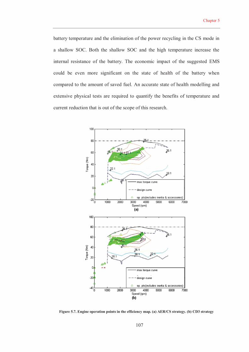
Chapter 5
107
battery temperature and the elimination of the power recycling in the CS mode in
a shallow SOC. Both the shallow SOC and the high temperature increase the
internal resistance of the battery. The economic impact of the suggested EMS
could be even more significant on the state of health of the battery when
compared to the amount of saved fuel. An accurate state of health modelling and
extensive physical tests are required to quantify the benefits of temperature and
current reduction that is out of the scope of this research.
Figure 5.7. Engine operation points in the efficiency map. (a) AER/CS strategy. (b) CD3 strategy
Chapter 5
108
As mentioned before, to have a fare comparison, the power-follower rules in both
suggested EMS and AER-CS strategies are similar. That is, the fuel reduction
recorded in Table 5-1 is only achieved by the charge management. The simplicity
of the suggested approach makes it a completely applicable EMS for vehicles
such as GM Volt, since the power management strategy is not changed by this
approach. The only input to the vehicle is when to shift from the EV mode to the
CS mode during a journey with a simple GPS feedback. Even the driver can make
the decision of shifting from the EV mode to the CS mode like the input button
designed for the GM Volt sister vehicle, Opel Ampera.
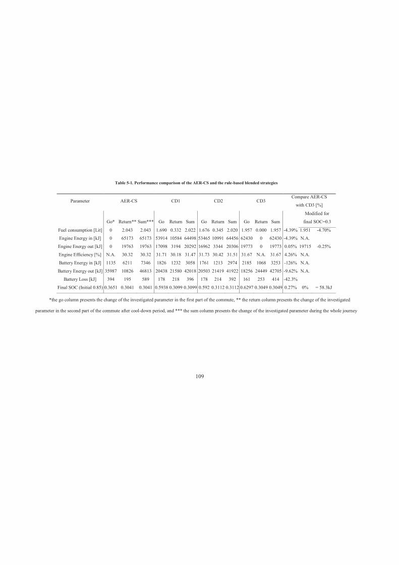
109
Table 5-1. Performance comparison of the AER-CS and the rule-based blended strategies
Parameter AER-CS CD1 CD2 CD3 Compare AER-CS
with CD3 [%]
Go* Return** Sum*** Go Return Sum Go Return Sum Go Return Sum
Modified for
final SOC=0.3
Fuel consumption [Lit] 0 2.043 2.043 1.690 0.332 2.022 1.676 0.345 2.020 1.957 0.000 1.957 -4.39% 1.951 -4.70%
Engine Energy in [kJ] 0 65173 65173 53914 10584 64498 53465 10991 64456 62430 0 62430 -4.39% N.A.
Engine Energy out [kJ] 0 19763 19763 17098 3194 20292 16962 3344 20306 19773 0 19773 0.05% 19715 -0.25%
Engine Efficiency [%] N.A. 30.32 30.32 31.71 30.18 31.47 31.73 30.42 31.51 31.67 N.A. 31.67 4.26% N.A.
Battery Energy in [kJ] 1135 6211 7346 1826 1232 3058 1761 1213 2974 2185 1068 3253 -126% N.A.
Battery Energy out [kJ] 35987 10826 46813 20438 21580 42018 20503 21419 41922 18256 24449 42705 -9.62% N.A.
Battery Loss [kJ] 394 195 589 178 218 396 178 214 392 161 253 414 -42.3%
Final SOC (Initial 0.85) 0.3651 0.3041 0.3041 0.5938 0.3099 0.3099 0.592 0.3112 0.3112 0.6297 0.3049 0.3049 0.27% 0% = 58.3kJ
*the go column presents the change of the investigated parameter in the first part of the commute, ** the return column presents the change of the investigated
parameter in the second part of the commute after cool-down period, and *** the sum column presents the change of the investigated parameter during the whole journey
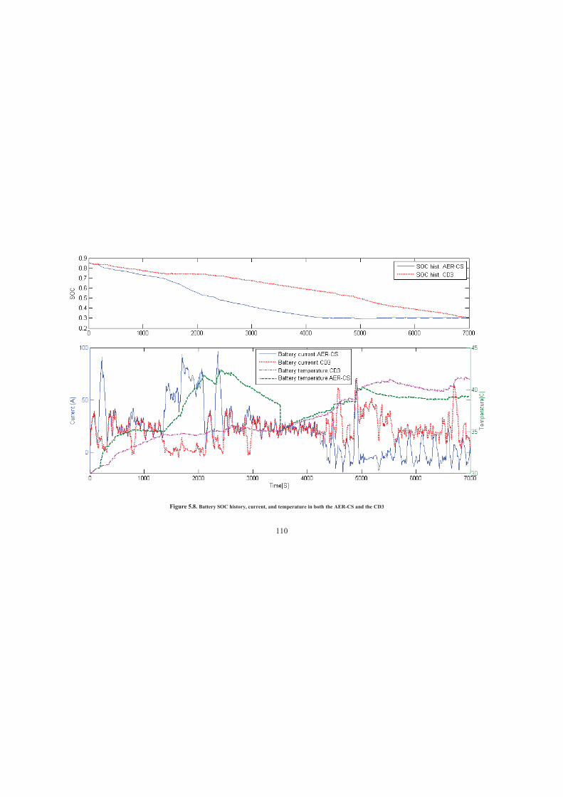
110
Figure 5.8. Battery SOC history, current, and temperature in both the AER-CS and the CD3
111
5.5 CONCLUSION
The blended mode energy management strategies are more efficient for the
EMS of PHEVs. When the blended mode EMS is defined for a PHEV, shifting
between the engine-on and off modes is frequent. Therefore, engine temperature
plummets while the engine is turned off. When the engine is running at
temperature lower than designated thermostatic temperature, its performance and
efficiency deteriorates.
A power-follower rule-based EMS operates the vehicle in an AER-CS EMS for
a simulated power-cycle. The same control rules also employed to operate the
vehicle in the developed blended mode EMS to have a fair comparison. In other
words, any reported improvement in the fuel economy of the vehicle is only the
result of the more efficient charge management of the vehicle rather than the
power management strategy. Based on the power-cycle of the simulated driving
scenario, an efficiency cycle was developed by assuming that the vehicle operates
based on the power follower rules, and the engine operates on confined optimal
operation line (COOL). To define a blended mode EMS, the efficiency cycle was
investigated in a three-step procedure to find the best sections to provide the
required engine energy share. The cold-factor calculation by means of the engine
thermal model was employed during the evolution of the efficiency cycle in the
last two steps of the strategy, CD2 and CD3. The effect of the second cold-start of
the vehicle for journeys with long cool-down periods was also investigated in the
last step of the EMS, CD3.

112
The simulation results for the modelled series PHEV, which has similar
specifications to GM Volt, show that the suggested CD energy management
strategy improves both the vehicle fuel economy and the battery health by
eliminating the significant power recirculation, reducing the battery load, and
accordingly its temperature.

113
CHAPTER 6
OPTIMAL INTEGRATED THERMAL AND ENERGY MANAGEMENT OF PHEVS
6.1 INTRODUCTION
The rule-based controller for EREV that considers the cold-factor fuel
consumption penalty and the cold start of the engine in the blended mode EMS
was introduced in Chapter 5. The rule-based controllers are practical, simple to
implement, and as explained in Section 5.4, the benefit of them is notable. In this
chapter, a new EMS with the dynamic modelling approach based on the theory of
dynamic programming (DP) is introduced to address three important aspects of
EMS of PHEVs. First, the method, based on DP, establishes a mathematical
Chapter 6
114
optimal solution of the modelled control problem. That is, if the modelling
process is in accordance to the physical reality of the control problem, the result
of the process could be accounted as the optimal benchmark for all other control
approaches. In practice, it is impossible to reach the limit found by the optimal
control theory; however, it is worth to access the benchmark solution. Second, the
DP method is appealing because the result is a global rather than a local optimal
solution. This is ideal for the charge management of PHEVs for known power-
cycles. The last but not the least reason is by adding a temperature as a state
variable into the optimal control problem formulation, it is possible to address the
optimal solution for the engine thermal management, and the battery charge
management, synchronously. This solution finds the best engine thermal
management to maximise the engine hot operation as well as the availability of
hot water from the engine coolant for the cabin heating propose.
In this chapter, first an introduction to the basics of the theory of dynamic
programing is given. Then, the formulation of the control problem and the
required cost function for the optimization process are discussed. Finally, the
results of a warm and a chilly day simulation, employing the suggested blended
mode EMS, are compared with those the conventional AER-CS strategy.
6.2 OPTIMAL CONTROL AND DYNAMIC PROGRAMMING
The objective of optimal control is to determine the control signals that satisfy
the physical constraints and also minimise (or maximise) a performance criterion
[100].

Chapter 6
115
6.2.1 Mathematical modelling for dynamic approach
The basic part of any control problem is to mathematically model the process.
The main objective of modelling is to find the simplest mathematical description
of the process which sufficiently describes dynamics of the system to all possible
inputs. A system is described by ordinary differential equations in state variable
form, where:
are state variables and
are control inputs, and the system could be described with n first order differential
equations:
By defining the state vector and input control vector the state
equation can be written [100]:
Eq. 6-1
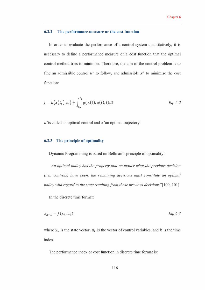
Chapter 6
116
6.2.2 The performance measure or the cost function
In order to evaluate the performance of a control system quantitatively, it is
necessary to define a performance measure or a cost function that the optimal
control method tries to minimize. Therefore, the aim of the control problem is to
find an admissible control to follow, and admissible to minimise the cost
function:
Eq. 6-2
is called an optimal control and an optimal trajectory.
6.2.3 The principle of optimality
Dynamic Programming is based on Bellman’s principle of optimality:
“An optimal policy has the property that no matter what the previous decision
(i.e., controls) have been, the remaining decisions must constitute an optimal
policy with regard to the state resulting from those previous decisions”[100, 101]
In the discrete time format:
Eq. 6-3
where is the state vector, is the vector of control variables, and is the time
index.
The performance index or cost function in discrete time format is:
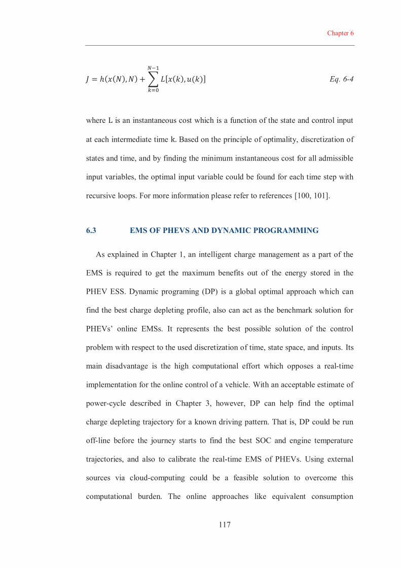
Chapter 6
117
Eq. 6-4
where is an instantaneous cost which is a function of the state and control input
at each intermediate time Based on the principle of optimality, discretization of
states and time, and by finding the minimum instantaneous cost for all admissible
input variables, the optimal input variable could be found for each time step with
recursive loops. For more information please refer to references [100, 101].
6.3 EMS OF PHEVS AND DYNAMIC PROGRAMMING
As explained in Chapter 1, an intelligent charge management as a part of the
EMS is required to get the maximum benefits out of the energy stored in the
PHEV ESS. Dynamic programing (DP) is a global optimal approach which can
find the best charge depleting profile, also can act as the benchmark solution for
PHEVs’ online EMSs. It represents the best possible solution of the control
problem with respect to the used discretization of time, state space, and inputs. Its
main disadvantage is the high computational effort which opposes a real-time
implementation for the online control of a vehicle. With an acceptable estimate of
power-cycle described in Chapter 3, however, DP can help find the optimal
charge depleting trajectory for a known driving pattern. That is, DP could be run
off-line before the journey starts to find the best SOC and engine temperature
trajectories, and also to calibrate the real-time EMS of PHEVs. Using external
sources via cloud-computing could be a feasible solution to overcome this
computational burden. The online approaches like equivalent consumption
Chapter 6
118
minimization strategies (ECMS), model predictive control, stochastic dynamic
programming, and heuristic strategies are locally optimal approaches which
cannot predict the optimal charge depleting strategy and engine thermal
management, accordingly.
6.3.1 Vehicle model
An inverse powertrain model analogous to the PHEV model described in
Chapter 3 is formulated as an optimal control problem in dynamic programming
to find the optimal charge depleting trajectory and EMS of the PHEV. Based on
the principle of optimality suggested by Bellman, the optimal path from any of its
intermediate steps to the final states corresponds to the terminal part of the entire
optimal solution [2, 49, 100, 102, 103]. For the series powertrain architecture, the
states are the battery charge, , and the engine internal temperature, , and
duration of engine operation since last start, , and the control vector is the
engine power, . In the discrete time format and using Eq. 6-3 :
Eq. 6-5
Eq. 6-6
Eq. 6-7
Electric power equilibrium at the power bus, depicted in Figure 3.2, could be
expressed in the form of Eq. 6-8. Power-cycle, the right side of Eq. 6-8, consists
Chapter 6
119
of the electric motor power, , and accessories loads, , and the heater
power demand, . When the engine is warm enough, , the heater
power demand, , could be supplied by the engine waste heat. As a
prerequisite of DP modelling, it is assumed that the power-cycle is predicted
based on the approach described in Chapter 3.
Eq. 6-8
where , , are ESS power, generator efficiency, and engine power
respectively.
There are some simplification assumptions for the battery subsystem of the DP
model of the vehicle compared to the model discussed in Chapter 3. First, it is
assumed that the resistance of the battery is independent of the SOC of the
battery. Moreover, the effect of temperature on the battery resistance is neglected.
Therefore, the battery thermal model is not considered. Dynamic programming
suffers from the curse of dimensionality. That is, adding each state variable
increases the computational load exponentially. Therefore, clever simplification
could limit the required computational effort to make the process reasonably
accurate and implementable in practice. Assuming that the ESS model is a perfect
open circuit voltage source in series with an internal resistance, and using Eq. 6-8
and Eq. 3-34 the relation between the state, , and the input variable, , is
described by Eq. 6-9. The motor power demand, , the accessories excluding
cabin heater power demand, , and the cabin heater power demand, ,
are fed into the DP model from the simulation results of the quasi-static model
Chapter 6
120
over the same power-cycle. In a series drivetrain, as the electric motor is the sole
vehicle traction provider, the control strategy does not affect the motor power
demand of the vehicle. Therefore, the results could be used in a dynamic approach
as well. The battery nominal voltage, , and resistance, , are kept similar to
quasi-static simulation.
Eq. 6-9
Using Eq. 6-5 and Eq. 6-9, the relation between the state, , and the input
variable, , in discrete format is:
Eq. 6-10
In this modelling, the simulation time step, , is assumed to be 1 second.
The internal engine temperature state, (k), is dependent on the input variable,
, with the heat transfer equations described in the engine thermal model.
Chapter 6
121
Similar equations that were described in Section 3.6.2., in discrete time format are
employed in the coding environment of Matlab instead of Simulink. Therefore,
temperatures at each nodes of the engine thermal model of Figure 3.5 can be
represented by following equations:
Eq. 6-11
Eq. 6-12
Eq. 6-13
Eq. 6-14
The last state variable, , which is the duration of the engine operation
before the last start is defined to prevent the frequent transitions between the
engine on and off modes. There is a threshold designed for minimum
duration, , that engine is kept operating. A lock inside the code prevents
Chapter 6
122
the engine to turn off before the minimum engine on time threshold. In this study,
the threshold is defined as 10 second.
Eq. 6-15
The optimization problem in discrete format is to find the control input, , to
minimize a cost function which represents the fuel consumption from the initial
time, , and states, , to the final time, , and states, .
From Eq. 6-4 in which the , the fuel cost function can be
defined as:
Eq. 6-16
where L is an instantaneous cost which is hereby defined as fuel consumption. It
is possible to add emission and its correspondent weighting factor to the cost
function. and are admissible PHEV states and control inputs, respectively,
which are defined based on the operational restrictions of the battery and the
engine-generator. could be defined as non-zero when the final SOC is
a soft constraint. The soft constraint means that the final SOC is acceptable in a
range rather than a fixed predefined SOC. Hence, a penalty to compensate the
Chapter 6
123
charge deviation should be considered. For HEVs with smaller battery, and for
short drive-cycle simulation, this might be useful which is not the case here.
6.3.2 Initialization of DP approach
As described in Section 5.2.1, the engine-generator operation is independent of
the vehicle speed in the series HEVs’ architecture. Therefore, the engine-
generator could operate over confined optimal operation line (COOL). (see Figure
5.2). Therefore, a bijective function can be defined between any engine power
demand, and fuel consumption.
In the dynamic programming initialization phase, the heater power demand can
be supplied by either the engine waste heat or electricity. Accordingly, two
corresponding change of charge against fuel consumption,
, are calculated for each time step by using COOL, Eq. 6-10,
and power-cycle. and define instantaneous
cost for any possible change in the state variable, , regardless of second
state variable, . In other words, and
define a one-to-one correspondence function between fuel consumption and
change of charge for each point of power-cycle for two cases of heater power
demand provided electrically or from engine waste heat respectively. Obviously,
for implementation purposes in Matlab, coding environment
and are saved in vector format for each time-step.
Chapter 6
124
6.3.3 Cost-to-go matrix
By implementing a forward DP approach, a cost-to-go matrix, J, is defined
recursively from the initial time-step via discretising the charge of battery and
time defined by the duration of drive-cycle. Any node on the cost-to-go matrix
represents the minimum cost to reach that specific charge and time from the
beginning of the journey. The time discretisation is , and the charge
discretisation in this simulation is . With the selected sizing of the
battery, the total charge capacity is:
Eq. 6-17
Eq. 6-18
The initial and final charges, as well as the maximum and minimum change of
charge in each time-step are used to determine the possible maximum and
Chapter 6
125
minimum charges of each time-step. This reduces dimensions of the recursive
loops for calculation of the cost-to-go matrix to the irregular hexagon shown in
schematic cost-to-go matrix in Figure 6.1. When the initial and final charges are
known, there are limited possible paths available in the cost-to-go matrix which
connects them. Indeed, maximum and minimum applicable charges of the battery
define the extremum horizontal boundaries. Two forward and backward
calculations are required to find the other four inclined boundaries. In forward
calculation, both maximum and minimum charge start from initial predefined
charge for the first column. For the next step, maximum and minimum possible
charge correspond to the charge of the battery if the engine operates at maximum
power or turns off, respectively. On the other hand, in the backward approach,
both maximum and minimum charge starts from final predefined charge for the
last column. For the next step backward, maximum and minimum possible charge
correspond to the charge of battery if engine turns off or operates at maximum
power, respectively. Eq. 6-20 and Eq. 6-21 represent forward and backward
calculation of the maximum and minimum charges in each step. The boundaries
of the possible charges in irregular hexagon in Figure 6.1. are defined by Eq. 6-22.

Chapter 6
126
In summary, only all possible paths from the initial to the final SOC are
investigated instead of finding the cost-to-go matrix for all the discretised charges
and times. This could significantly reduce the calculation time for large battery
and for drive-cycles longer than the AER of PHEVs.

Chapter 6
127
`
ForwardCalculation
Time (t)
Cha
rge
Ch
Initial Charge
Final Charge
Max. allowedCharge
Min. AllowedCharge
uN
uch
u1
ch=1...N
Max. applicable charge intime step
Min. applicable charge intime step
),(),(
),(),(
ChkPathChkt
ChkTChkJ
index
onEng
i
Min. CostInternal Engine Temp.Duration of the Eng. Operation Since Last RestartOptimal Path Index From Previous Step
Optimal path
Figure 6.1. Graphical representation of cost-to-go matrix
Based on the Bellman’s recursive equation approach, the cost function, Eq.
6-23 is solved by an interpolation method to find the minimum cost to reach a
specific node from all possible charges of the previous time step considering both
minimum engine-on-time and cold-factor. Cold-factor relates the cost function to
the second state variable, , using Eq. 6-25. Also, minimum engine-on-time
defines the minimum duration that the engine is permitted to turn off again after it
starts. This prevents excessive transient operation of the engine which is generally
associated with low efficiency and high emission. All possible charges, , costs,
, and fuel consumptions, and , are shown in vector format
in Eq. 6-23. The engine on-time, , defining duration of the engine

Chapter 6
128
operation, and the engine internal temperature, , derived from the thermal model
of the engine, are also calculated and saved for each node. Two inequality
functions in Eq. 6-23 define the condition for supplying the heater power demand
by the engine waste heat and prevent the engine to turn off before a minimum
engine-on-time threshold. For each node of the cost-to-go matrix, the index of the
ascendant node defining the optimal path to the specific node is also saved. This is
required to identify the initial conditions for cost, , thermal model,
, engine on time, for forward cost-to-go calculations and
also to find the SOC trajectory in the backward phase of DP. The schematic
calculation of cost-to-go for each node is depicted in Figure 6.2.
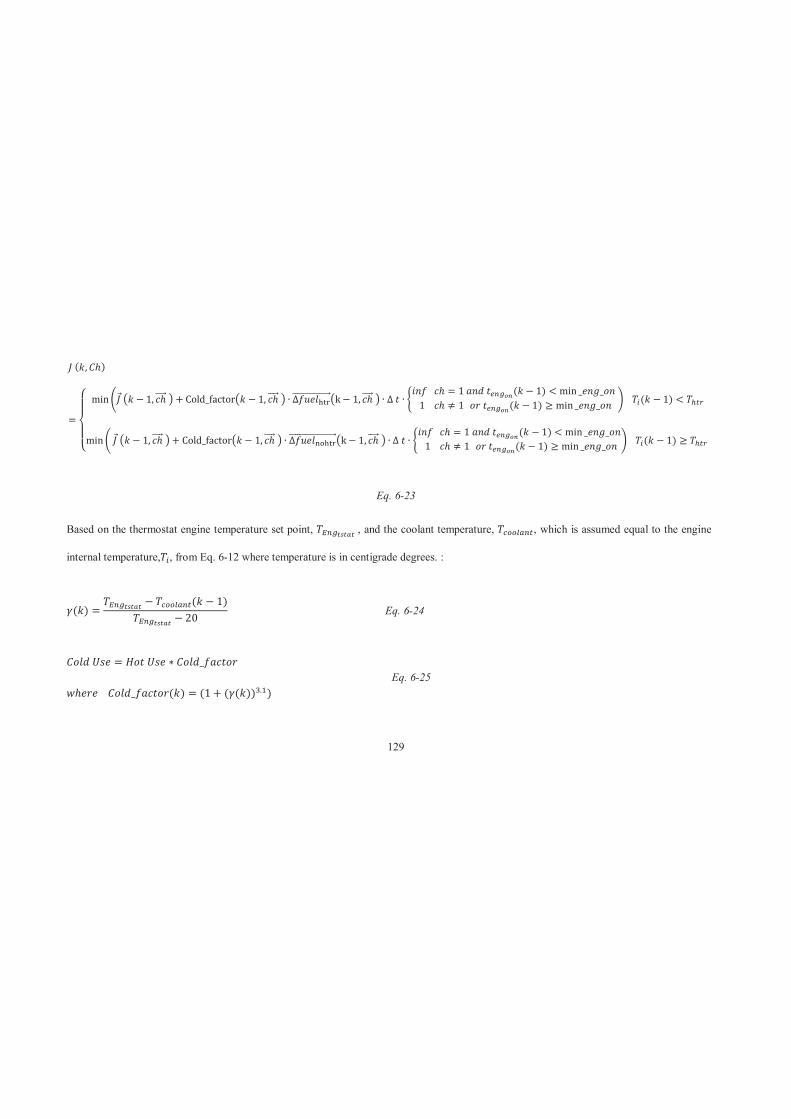
129
Eq. 6-23
Based on the thermostat engine temperature set point, , and the coolant temperature, , which is assumed equal to the engine
internal temperature, , from Eq. 6-12 where temperature is in centigrade degrees. :
Eq. 6-24
Eq. 6-25
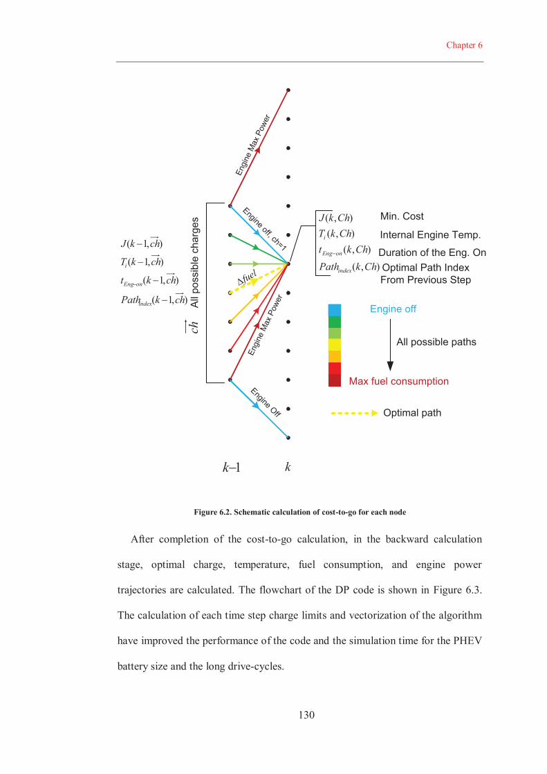
Chapter 6
130
Engine Off
Engine off, ch=1En
gine
Max
Powe
r
Engi
neM
axPo
wer
1k k
),(),(
),(),(
ChkPathChkt
ChkTChkJ
index
onEng
i
Min. Cost
Internal Engine Temp.
Duration of the Eng. OnOptimal Path IndexFrom Previous Step
chAl
lpos
sibl
ech
arge
s
),1(
),1(
),1(
),1(
chkPath
chkt
chkT
chkJ
index
onEng
i
fuel
Engine off
Max fuel consumption
Optimal path
All possible paths
Figure 6.2. Schematic calculation of cost-to-go for each node
After completion of the cost-to-go calculation, in the backward calculation
stage, optimal charge, temperature, fuel consumption, and engine power
trajectories are calculated. The flowchart of the DP code is shown in Figure 6.3.
The calculation of each time step charge limits and vectorization of the algorithm
have improved the performance of the code and the simulation time for the PHEV
battery size and the long drive-cycles.
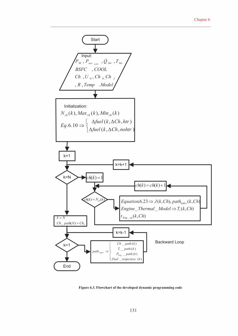
Chapter 6
131
Start
ModelTempR
ChChUChCOOLBSFC
TQPP
f
htrhtraccM nohtr
.,,
,,,
,,,
,00
Input:
Initialization:
),,(),,(
10.6.
)(),(),(
nohtrChkfuelhtrChkfuel
Eq
kMinkMaxkN chchch
k=1
k=N
)()( kNkch ch
1)(kch
k=k+1
1)()( kchkch
),(),(__
),(),,(23.6.
_ ChktChkTModelThermalEngine
ChkpathChkJEquation
onEng
i
index
k=k-1
k=1
fChNpathChNk
)(_
)(_)(_
)(_)(_
ktrajectoryFuelkpathP
kpathTkpathCh
pathEng
iindex
End
Backward Loop
Figure 6.3. Flowchart of the developed dynamic programming code

Chapter 6
132
6.3.4 Forward DP instead of backward DP
Generally, dynamic programming is known as a backward approach. That is, in
case of energy management strategy of HEVs and PHEVs, the calculation of cost-
to-go matrix starts from the end of journey back to the initial point. There are two
main reasons that make it necessary to use forward instead of backward DP. First,
the initial conditions at the end of the journey are unknown, thus the thermal
model equations cannot be solved in a backward manner. In the engine thermal
model, the engine mass is lumped to four temperatures, cylinder, , engine
interior, , engine exterior, , and hood temperature, . If a backward
approach is selected, the initial conditions of the heat transfer equations are
unknown at the end of the journey. In addition, when the coolant reaches the
thermostat temperature, the radiator heat transfer rate, , as an extra
unknown, is added if the thermal model is to be solved backward. Therefore, it is
impossible to form the cost-to-go matrix with backward approach if the
temperature as a state variable is considered.
6.4 SIMULATION RESULTS
To prove the significance of temperature on the optimal EMS of PHEVs, two
80 km driving scenarios simulating warm and chilly days are defined. Simulations
conducted to find the optimal battery charge and engine power trajectories using
the developed DP code. The results are compared against those of the AER-CS
and DP EMS methods which neglect the cold-factor, engine cold start, and
heater/AC power demands. The name “DP with cold-factor” is selected for the
developed dynamic programming-based method proposed in Section 6.3. The
Chapter 6
133
formulation of “DP without cold-factor” is similar, but does not consider the
engine temperature as a state variable in the control problem. Therefore, for the
“DP without cold-factor”, the cost function in Eq. 6-23 is defined without
considering the cold-factor and the heater power demand inequality function. To
show the real fuel consumption, the cold-factor multiplied by the cost. The cold-
factor is not considered in the minimization function (see Eq. 6-26) of “DP
without cold-factor”.
Eq. 6-26
6.4.1 Driving scenario
The drive-cycle represents a typical work-home commute which starts in a
suburban area, characterized by UDDS, then continues on a highway, simulated
by HWFET, and finally arrives to downtown urban area, UDDS. Destination
elevation is around 400 meters higher than the starting point. For the warm day
driving scenario, vehicle stops during working hours and the engine cools down to
the ambient temperature. The return journey is the mirror of the defined driving
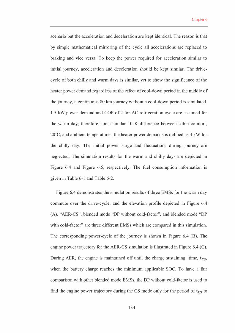
Chapter 6
134
scenario but the acceleration and deceleration are kept identical. The reason is that
by simple mathematical mirroring of the cycle all accelerations are replaced to
braking and vice versa. To keep the power required for acceleration similar to
initial journey, acceleration and deceleration should be kept similar. The drive-
cycle of both chilly and warm days is similar, yet to show the significance of the
heater power demand regardless of the effect of cool-down period in the middle of
the journey, a continuous 80 km journey without a cool-down period is simulated.
1.5 kW power demand and COP of 2 for AC refrigeration cycle are assumed for
the warm day; therefore, for a similar 10 K difference between cabin comfort,
20˚C, and ambient temperatures, the heater power demands is defined as 3 kW for
the chilly day. The initial power surge and fluctuations during journey are
neglected. The simulation results for the warm and chilly days are depicted in
Figure 6.4 and Figure 6.5, respectively. The fuel consumption information is
given in Table 6-1 and Table 6-2.
Figure 6.4 demonstrates the simulation results of three EMSs for the warm day
commute over the drive-cycle, and the elevation profile depicted in Figure 6.4
(A). “AER-CS”, blended mode “DP without cold-factor”, and blended mode “DP
with cold-factor” are three different EMSs which are compared in this simulation.
The corresponding power-cycle of the journey is shown in Figure 6.4 (B). The
engine power trajectory for the AER-CS simulation is illustrated in Figure 6.4 (C).
During AER, the engine is maintained off until the charge sustaining time, ,
when the battery charge reaches the minimum applicable SOC. To have a fair
comparison with other blended mode EMSs, the DP without cold-factor is used to
find the engine power trajectory during the CS mode only for the period of to
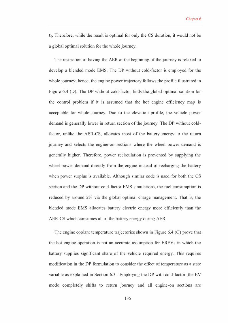
Chapter 6
135
. Therefore, while the result is optimal for only the CS duration, it would not be
a global optimal solution for the whole journey.
The restriction of having the AER at the beginning of the journey is relaxed to
develop a blended mode EMS. The DP without cold-factor is employed for the
whole journey; hence, the engine power trajectory follows the profile illustrated in
Figure 6.4 (D). The DP without cold-factor finds the global optimal solution for
the control problem if it is assumed that the hot engine efficiency map is
acceptable for whole journey. Due to the elevation profile, the vehicle power
demand is generally lower in return section of the journey. The DP without cold-
factor, unlike the AER-CS, allocates most of the battery energy to the return
journey and selects the engine-on sections where the wheel power demand is
generally higher. Therefore, power recirculation is prevented by supplying the
wheel power demand directly from the engine instead of recharging the battery
when power surplus is available. Although similar code is used for both the CS
section and the DP without cold-factor EMS simulations, the fuel consumption is
reduced by around 2% via the global optimal charge management. That is, the
blended mode EMS allocates battery electric energy more efficiently than the
AER-CS which consumes all of the battery energy during AER.
The engine coolant temperature trajectories shown in Figure 6.4 (G) prove that
the hot engine operation is not an accurate assumption for EREVs in which the
battery supplies significant share of the vehicle required energy. This requires
modification in the DP formulation to consider the effect of temperature as a state
variable as explained in Section 6.3. Employing the DP with cold-factor, the EV
mode completely shifts to return journey and all engine-on sections are

Chapter 6
136
concentrated before the cool-down period. This eliminates the second cold start
warm-up procedure which leads to cold engine operation and consequently the
cold-factor penalty. The DP with cold-factor selects the first section of the
commute for the blended mode operation, as the battery energy is adequate to run
the downhill return journey in the EV mode. The overall engine efficiency for the
whole journey is higher when one extra engine warm-up is eliminated. That is, the
effect of warmer engine operation overcompensate the reduction of the vehicle
efficiency because of the engine operation in the lower power demand when
compared with the DP without cold-factor. Our proposed “DP with cold-factor”
approach improves the fuel economy of the vehicle by 3.2% compared with the
AER-CS EMS. Therefore, it improves the performance of the DP without cold-
factor by 1.2%. This result simulates inaccuracy of relying on the DP without
cold-factor for PHEVs with large battery as the optimal EMS benchmark. In
addition, as described in the introduction section, the cold operation of the engine
and catalyst converter has a major role in the emission of the vehicle. Therefore,
the environmental impact of the emission reduction by elimination of the second
cold-start may outweigh the amount of fuel saved. According to the simulation
conducted in ADVISOR, the HC, CO, and NOx emissions are reduced by almost
27%, 11%, and 17% respectively compared to the AER-CS simulation (see Table
6-1).
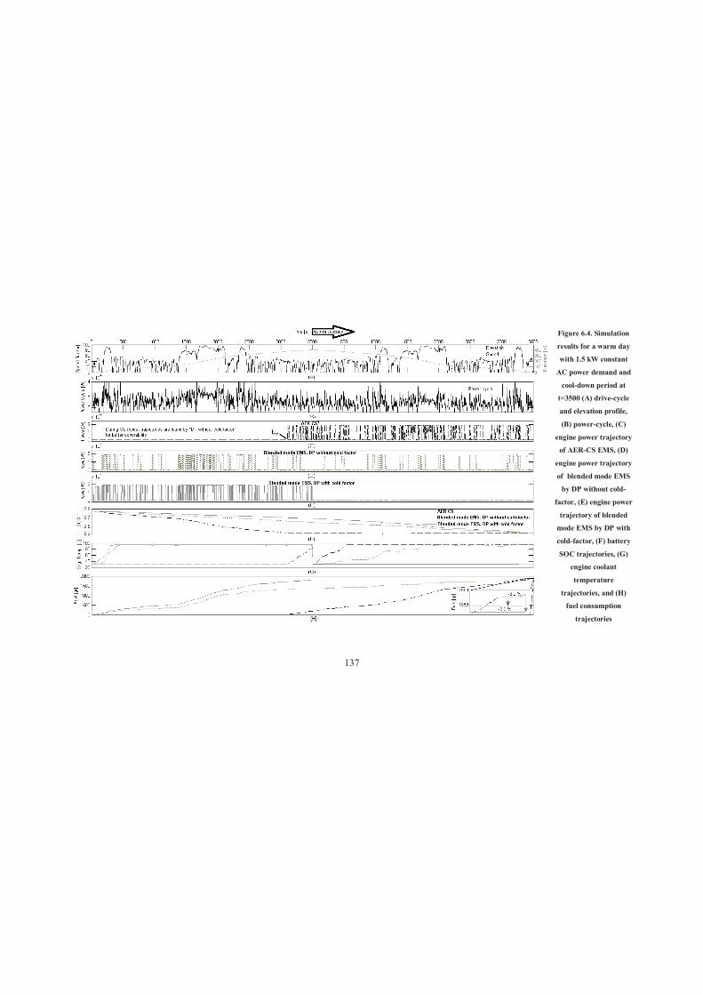
137
Figure 6.4. Simulation
results for a warm day
with 1.5 kW constant
AC power demand and
cool-down period at
t=3500 (A) drive-cycle
and elevation profile,
(B) power-cycle, (C)
engine power trajectory
of AER-CS EMS, (D)
engine power trajectory
of blended mode EMS
by DP without cold-
factor, (E) engine power
trajectory of blended
mode EMS by DP with
cold-factor, (F) battery
SOC trajectories, (G)
engine coolant
temperature
trajectories, and (H)
fuel consumption
trajectories
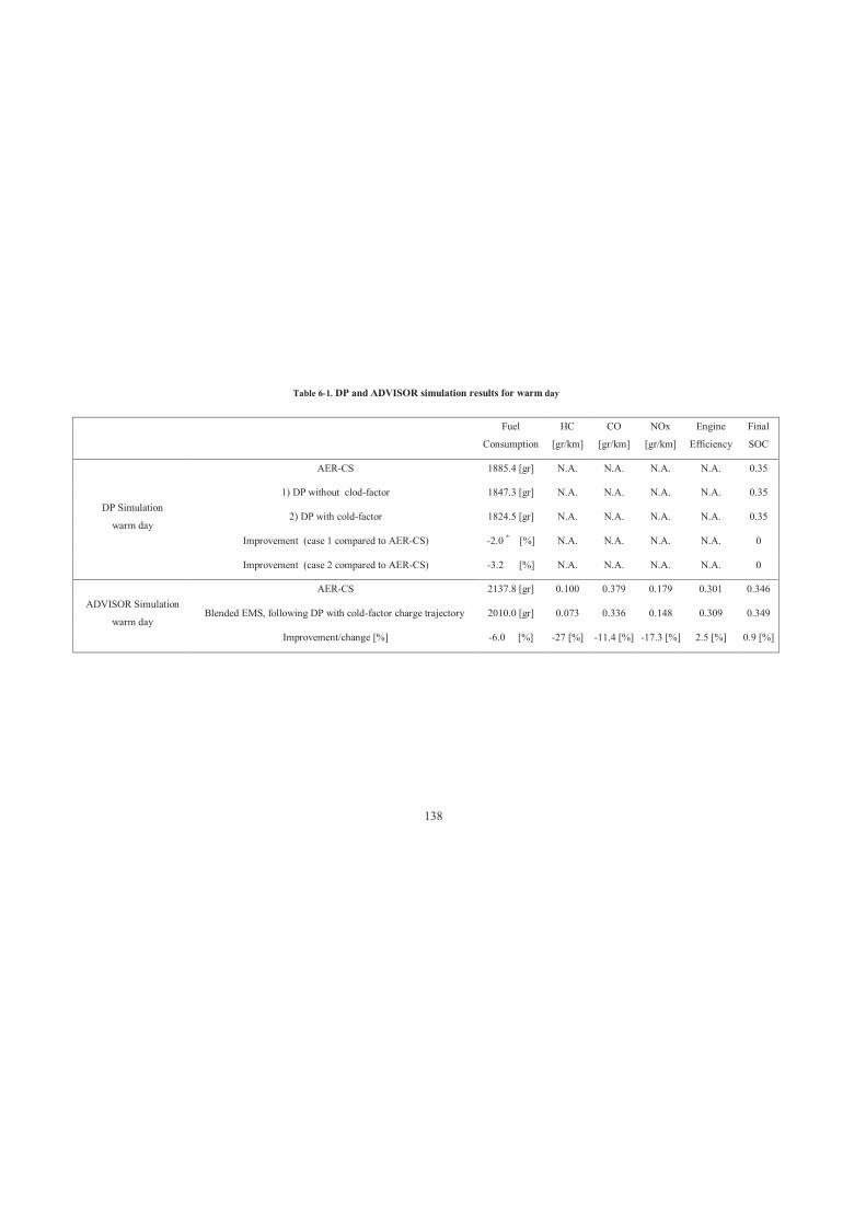
138
Table 6-1. DP and ADVISOR simulation results for warm day
Fuel
Consumption
HC
[gr/km]
CO
[gr/km]
NOx
[gr/km]
Engine
Efficiency
Final
SOC
DP Simulation
warm day
AER-CS 1885.4 [gr] N.A. N.A. N.A. N.A. 0.35
1) DP without clod-factor 1847.3 [gr] N.A. N.A. N.A. N.A. 0.35
2) DP with cold-factor 1824.5 [gr] N.A. N.A. N.A. N.A. 0.35
Improvement (case 1 compared to AER-CS) -2.0 * [%] N.A. N.A. N.A. N.A. 0
Improvement (case 2 compared to AER-CS) -3.2 [%] N.A. N.A. N.A. N.A. 0
ADVISOR Simulation
warm day
AER-CS 2137.8 [gr] 0.100 0.379 0.179 0.301 0.346
Blended EMS, following DP with cold-factor charge trajectory 2010.0 [gr] 0.073 0.336 0.148 0.309 0.349
Improvement/change [%] -6.0 [%] -27 [%] -11.4 [%] -17.3 [%] 2.5 [%] 0.9 [%]

Chapter 6
139
The engine operation trajectories of the AER-CS EMS of a full electric cabin
heater vehicle and a vehicle in which the heater power is supplied by both the
battery and the engine waste heat are compared in Figure 6.5 (B-C). The
significant 34% improvement in the fuel economy could be realised by employing
the waste heat of the engine like conventional vehicles. Based on the author’s
knowledge gained at 2011 Frankfurt motor show, the GM Volt cabin heater is an
all-electric, while Opel has solved the issue for the Ampera models. The engine
power path shown in Figure 6.5 (D) is derived based on the DP EMS with cold-
factor for a vehicle with both engine coolant and electric heater. Figure 6.5 (F)
illustrates how the optimal EMS found by the DP with cold-factor tends to keep
the engine warm for longer duration to provide the cabin heater power demand
free of cost. Indeed, holding the temperature not exactly at the thermostat
temperature comes at a cost of a reduction in engine efficiency defined by the
cold-factor. The optimal EMS based on DP compromises between maximum
availability of the hot water from the engine by distributing engine-on sections
during the journey and the effect of cold-factor on the engine efficiency. Referring
to Table 6-2, for ADVISOR simulation, 14% improvement in the fuel economy is
achieved, while the engine efficiency is reduced by 3% because of the operation at
temperatures below thermostat set-point. That is, the amount of fuel saved by
keeping the engine warm outweighs the drawback of its operation at not exactly
the thermostat temperature set-point. When heater operation is required for cold
weather, the DP with cold-factor method finds the optimal trajectory of state
variables, ESS charge and accordingly the engine internal temperature, to
minimise the fuel consumption cost function. It is interesting how the optimal
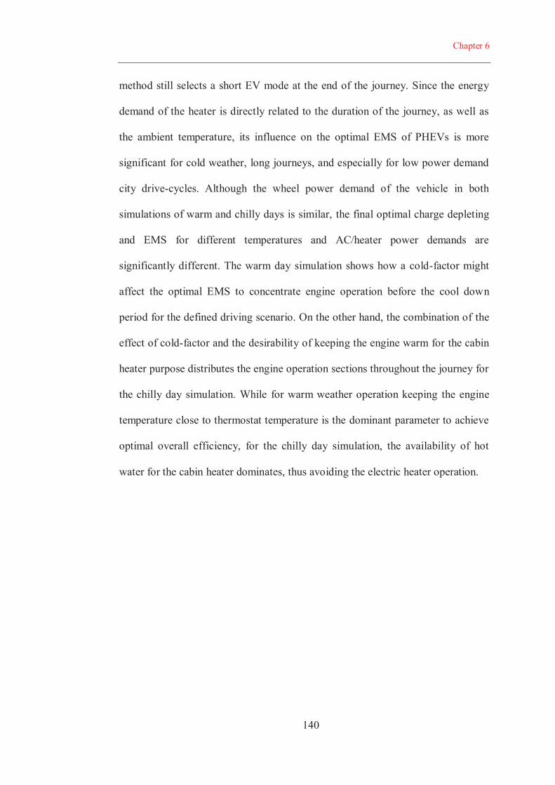
Chapter 6
140
method still selects a short EV mode at the end of the journey. Since the energy
demand of the heater is directly related to the duration of the journey, as well as
the ambient temperature, its influence on the optimal EMS of PHEVs is more
significant for cold weather, long journeys, and especially for low power demand
city drive-cycles. Although the wheel power demand of the vehicle in both
simulations of warm and chilly days is similar, the final optimal charge depleting
and EMS for different temperatures and AC/heater power demands are
significantly different. The warm day simulation shows how a cold-factor might
affect the optimal EMS to concentrate engine operation before the cool down
period for the defined driving scenario. On the other hand, the combination of the
effect of cold-factor and the desirability of keeping the engine warm for the cabin
heater purpose distributes the engine operation sections throughout the journey for
the chilly day simulation. While for warm weather operation keeping the engine
temperature close to thermostat temperature is the dominant parameter to achieve
optimal overall efficiency, for the chilly day simulation, the availability of hot
water for the cabin heater dominates, thus avoiding the electric heater operation.
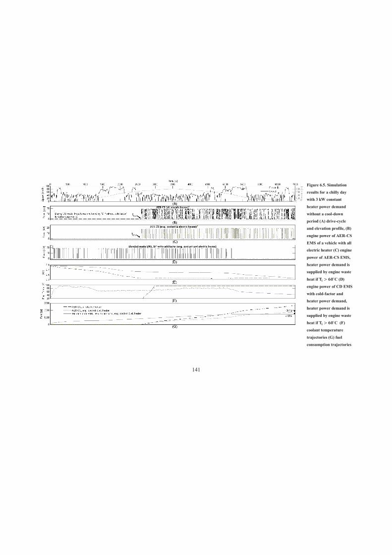
141
Figure 6.5. Simulation
results for a chilly day
with 3 kW constant
heater power demand
without a cool-down
period (A) drive-cycle
and elevation profile, (B)
engine power of AER-CS
EMS of a vehicle with all
electric heater (C) engine
power of AER-CS EMS,
heater power demand is
supplied by engine waste
heat if ˚C (D)
engine power of CD EMS
with cold-factor and
heater power demand,
heater power demand is
supplied by engine waste
heat if ˚C (F)
coolant temperature
trajectories (G) fuel
consumption trajectories
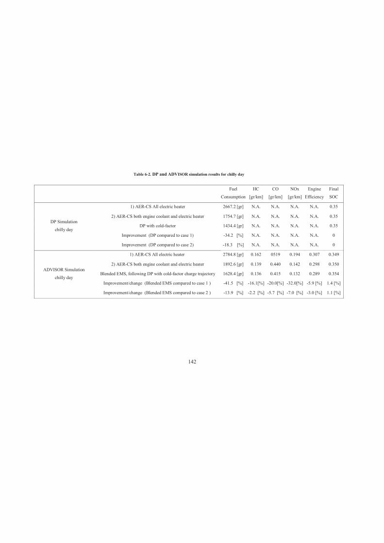
142
Table 6-2. DP and ADVISOR simulation results for chilly day
Fuel
Consumption
HC
[gr/km]
CO
[gr/km]
NOx
[gr/km]
Engine
Efficiency
Final
SOC
DP Simulation
chilly day
1) AER-CS All electric heater 2667.2 [gr] N.A. N.A. N.A. N.A. 0.35
2) AER-CS both engine coolant and electric heater 1754.7 [gr] N.A. N.A. N.A. N.A. 0.35
DP with cold-factor 1434.4 [gr] N.A. N.A. N.A. N.A. 0.35
Improvement (DP compared to case 1) -34.2 [%] N.A. N.A. N.A. N.A. 0
Improvement (DP compared to case 2) -18.3 [%] N.A. N.A. N.A. N.A. 0
ADVISOR Simulation
chilly day
1) AER-CS All electric heater 2784.8 [gr] 0.162 0519 0.194 0.307 0.349
2) AER-CS both engine coolant and electric heater 1892.6 [gr] 0.139 0.440 0.142 0.298 0.350
Blended EMS, following DP with cold-factor charge trajectory 1628.4 [gr] 0.136 0.415 0.132 0.289 0.354
Improvement/change (Blended EMS compared to case 1 ) -41.5 [%] -16.1[%] -20.0[%] -32.0[%] -5.9 [%] 1.4 [%]
Improvement/change (Blended EMS compared to case 2 ) -13.9 [%] -2.2 [%] -5.7 [%] -7.0 [%] -3.0 [%] 1.1 [%]
143
Simulations also show another interesting result that is the engine power has
limited fluctuations around the most efficient engine operation point regardless of
the changes in the power demand (see Figure 6.6). This implies that the optimal
operation of the vehicle dominantly depends on the engine efficient operation.
Since the large PHEV ESS benefits from parallel modules, its internal resistance
compared to the conventional HEVs is significantly lower. Therefore, the
electrical waste in PHEV ESS is reduced accordingly.
Figure 6.6. A superimposed selected section of Figure 6.4(B) and (D)
6.5 REAL-TIME IMPLEMENTATION
Although the DP approach could not be implemented in a real-time control of a
vehicle, the optimal charge depleting trajectory for a known driving scenario
could help calibrate the EMS in an online fashion. That is, the real-time EMS tries
to implement the same optimal charge management by following the charge
trajectory found by the DP approach. Particularly, the DP approach can suggest
the best sections of the journey to run on the pure EV mode for EREV. The
144
charge trajectory should be followed based on a position feedback from the
vehicle in a journey instead of the time domain using a GPS. In the following, it is
described how effectively only the knowledge of optimal charge trajectory
regardless of the type of real-time EMS could significantly improve the
performance of PHEV.
The rule based power follower described in Section 5.3 controls the vehicle in
ADVISOR simulation tool for the same driving scenario explained in the previous
section. The ADVISOR model is manipulated to simulate the heater and AC loads
and the effect of heater cool-down on engine thermal model. Also, the vehicle
control unit is redesigned to sustain the ESS SOC around charge depleting
trajectory derived from the DP approach by using a feedback control. The results
are shown in Figure 6.7, Table 6-1, and Table 6-2. By following the charge
trajectory found by DP with cold-factor, however, the battery to engine energy
ratio during the journey is remained similar to the DP optimal trend. This results
in almost a similar engine temperature trajectory. The slight deviation between the
temperature trajectories of DP with cold-factor and the simulations is a result of
the difference between the engine operation trajectories and the difference
between the heater cooling effect on engine thermal model of the DP and
ADVISOR. Due to discretization, the heater power demand is defined step-wise
for the DP model which shifts at a defined threshold. Yet, the heater cooling effect
on engine thermal model of ADVISOR is defined by a linear equation so the
cooling effect continues for all temperatures.
The amount of fuel saved for the chilly day simulation proves the significant
drawback of using only electric heater. Improvement in fuel efficiency of vehicle

145
could be even considerably increased for extreme low temperatures. Besides, the
emission reduction is another positive aspect of an EMS considering temperature
noise factor; particularly, when an unnecessary cold-start/warm-up of the engine
and catalytic converter is eliminated.
Figure 6.7. (A) Comparison of the coolant temperature trajectories in ADVISOR and DP with cold-
factor simulations for (A) Warm day (B) Chilly day
6.6 CONCLUSION
The influence of the temperature noise factor on the optimal energy
management strategy of PHEVs was demonstrated in this Chapter via developing
a Dynamic Programming-based approach. DP based on Bellman’s principle of
optimality derives the optimal charge depleting trajectory of the battery. This
coincides with the optimal thermal management of the engine for minimum fuel
consumption, while maximizing employing engine waste heat for cabin warming
instead of the battery electricity. The simulation results prove that temperature
considerably changes the optimal EMS and accordingly fuel consumption and
emission of PHEVs even for identical drive-cycles. A practical approach to

146
implement the result of the optimal EMS for calibrating a real-time EMS that
addresses the realistic disturbances of real world driving was also proposed.
147
CHAPTER 7
CONCLUSION AND FUTURE WORK
7.1 CONCLUSION
This thesis focused on optimisation of energy management strategy for plug-in
hybrid electric vehicles. The energy management strategy tries to control the
energy flow in the powertrain components of PHEVs to find the most efficient
energy path to provide the vehicle power demand. Unlike HEVs in which the
engine is the sole source of energy, grid charged battery alongside the engine adds
an extra energy path to provide vehicle power demand in PHEVs. Therefore, a
Chapter 7
148
battery charge management strategy is incorporated into the EMS of PHEVs to
fully harness the benefits of the extra energy source.
All available approaches, implementable for the EMS of PHEVs, were
categorised in Chapter 2. Among them, two different methods: (i) a rule-
based/deterministic, and (ii) an optimization-based/deterministic were selected to
be investigated in this research. The deterministic methods tackle the control
problem globally (i.e. for the whole journey). Hence, they are suitable choices for
addressing the optimal battery charge management. The rule-based approaches are
easily implementable while the optimization-based approaches can be used as
optimal solutions.
Different modelling and simulation methods available in the literature were
introduced in Chapter 3. The method selected for this research was also outlined
and different vehicle components models were discussed. The vehicle components
were sized to simulate an EREV with 64 km AER capability similar to GM Volt.
The battery energy source reduces the engine load and during the EV mode engine
is turned off for long periods. Therefore, the engine is more likely to operate cold
compared with conventional HEVs. This leads to lower engine efficiency and
higher emission. In addition, while the engine is cold, the power demand of the
cabin heater needs to be supplied by battery. An engine thermal model and a cold-
factor fuel consumption penalty were incorporated into the vehicle model to
investigate these phenomena. Existing studies on the EMS of PHEVs mostly
focus on the improvement of fuel efficiency based on hot engine characteristics
neglecting the effect of temperature on the engine performance and vehicle power
demand.
Chapter 7
149
The implementation of globally optimal energy management strategies based
on the deterministic approaches is only feasible when an accurate prediction of
power-cycle is available. Many noise factors affect both drivetrain power demand
and vehicle performance even in identical drive-cycles. In Chapter 4, the effect of
each noise factor was investigated and the power-cycle library was proposed to
improve the accuracy of the power-cycle prediction. A library of power-cycles
provides the required information about the journey in both time and spatial
domains, which helps to predict the power-cycle affected by the environmental
noise-factors before a journey starts. PHEVs employ an in-built control strategy
defined by OEM, normally an AER-CS similar to what has been designed for GM
Volt or Toyota Prius PHEV. However, for known power-cycles, defined later by
each vehicle owner, a more sophisticated energy management strategy would be
implemented.
Chapter 5 introduced a blended mode rule-based EMS for the modelled
vehicle. A driving scenario was simulated and fuel economy of the vehicle with a
conventional AER-CS EMS was compared against that of the suggested rule-
based EMS. Based on the power-cycle of the simulated driving scenario, an
efficiency cycle was developed. The efficiency cycle was investigated in a three-
step procedure to find the best sections to provide the required engine energy
share. One of the characteristics of the blended mode EMS is frequent shifting
between the engine-on and off modes. Therefore, the effect of the engine cooler
operation on its performance should be investigated. The cold-factor calculation
by means of the engine thermal model was employed to modify the efficiency
cycle in the last two steps of the EMS. Moreover, the effect of the second cold-
Chapter 7
150
start of the vehicle for journeys with long cool-down periods was also
investigated. The result of the EMS was a sub-optimal solution that defines the
best section of the journey to shift from the EV to CS mode. The rule-based
approach is a practical and easily implementable approach due to the limited
computational effort required.
In Chapter 6, optimal EMS control problem was formulated by using the
dynamic programming method. One input variable, engine power, and three state
variables, battery charge, engine internal temperature, and engine operation time
were employed for formulating of the control problem. The cost function of the
dynamic programming method correlates fuel economy of the vehicle to all these
three state variables. The optimal battery charge depleting and the engine
temperature trajectories secure globally optimal fuel economy for a prescribed
journey with specific environmental conditions. The proposed approach also
maximises the usage of the engine waste heat for cabin warming instead of the
battery electricity in cold weather conditions. The simulation results proved that
temperature considerably changes the optimal EMS, and accordingly the fuel
consumption and emissions of PHEVs even for identical drive-cycles. A practical
approach to implement the result of the optimal EMS for calibrating a real-time
EMS was also proposed.
The simulations show significant improvement in the fuel efficiency of PHEVs
with integration of the engine thermal management and EMS. Around 4.7%
improvement in the fuel economy is achieved by the rule-based EMS, described
in Chapter 5, according to the simulation of a warm day commute. The power
recirculation, one of the major reasons for the battery degradation, is also reduced

Chapter 7
151
significantly so that the amount of battery charging energy is declined by 126%
during the commute simulation. Since the suggested EMS forces the engine to
provide the required power of the drivetrain in the most vigorous part of the
journey, the battery energy is consumed during a longer period and logically at
lower power. Therefore, the maximum current and battery temperature, one the
major reasons for battery degradation, are also declined accordingly. The
deterministic optimal method, described in Chapter 6, provides even better results
compared to the rule-based EMS. 6% and 13.9% improvement in the fuel
economy of the vehicle in warm and chilly day simulations are recorded
respectively.
7.2 FUTURE WORK
Some potential future directions that merit further study are listed as follows:
As described in Section 3.6.2, the cold-factor fuel consumption is
formulated mathematically based on the internal combustion engine
coolant temperature. Sensibility of the engine efficiency to its internal
temperature is not uniform at all speeds and torques. Therefore, the best
way to formulate the engine efficiency at each specific speed, torque, and
temperature is via engine dynamometry tests. In other words, it is more
accurate to rely on the efficiency maps of the engine at different
temperatures rather than using a single variable cold-factor function. This
helps avoid specific torque-speed operation points that are more sensitive
to cold engine operation during the transitional warm-up procedure.
Chapter 7
152
Prediction procedure of power-cycle with the aim of the power-cycle
library was described in Chapter 4. As discussed, power-cycle can be
predicted individually for each vehicle. In case of availability of a PHEV,
it is possible to equip it with required sensors, schematically shown in
Figure 4.1. As control by wire is completely dominant in PHEVs, there is
not any expensive equipment required for this purpose. This helps
evaluate sensitivity and accuracy of the power-cycle prediction process in
real-world operation condition.
In case of availability of a PHEV like GM Volt, Opel Ampera, or Prius
PHEV, the performance of the suggested rule-based EMS can be
evaluated easily. As explained in Chapter 5, the rule-based EMS defines
the best sections to operate in the EV or CS modes for a journey. Since a
manual EV mode selection is available in these vehicles, it is possible to
manually select the EV mode sections based on the rule-based EMS
suggestions.
Here the optimization procedure cost function is only defined based on
fuel consumption. However the cost function could be defined based on
both fuel economy and emission. Since fuel consumption and emission
do not follow similar dynamic, reduction of fuel consumption could
result in an increase in emission and vice versa. The thermal dynamic of
the catalytic converter is also should be modelled in optimisation process.
The appropriate weighting factors should be defined to compromise
between emission and fuel consumption.

Bibliography
153
BIBLIOGRAPHY
[1] M. Ehsani, Y. Gao, S. E. Gay, and A. Emadi, Modern electric, hybrid
electric, and fuel cell vehicles : fundamentals, theory, and design: CRC,
2005.
[2] L. Guzzella and A. Sciarretta, Vehicle propulsion systems: introduction to
modeling and optimization, Second ed.: Springer, 2007.
[3] C. Mi, M. Abul Masrur, and D. W. Gao, Hybrid electric vehicles: principles
and applications with practical perspectives: John Wiley & Sons, 2011.
[4] I. Husain, Electric and Hybrid Vehicles: Design Fundamentals, Second ed.:
CRC Press 2010.
[5] J. Barnes, M. v. Walwijk, and C. Saricks, Hybrid and electric vehicles: The
electric drive gains momentum : Progress towards sustainable
transportation: International Energy Agency, 2007.

Bibliography
154
[6] J. Tollefson, "Charging up the future," Nature, vol. 456, pp. 436–440, Nov.
2008.
[7] M. Yamamoto, "Development of a Toyota plug-in hybrid vehicle," in SAE
World Congress & Exhibition, Detroit, MI, USA, 2010.
[8] R. Zito, "EVs and Travel Behavior change," Institute for Sustainable
Systems and Technologies -Transport Systems, Adelaide 2010.
[9] IEEE-USA Board of Directors. Position Statement: Plug-in Electric Hybrid
Vehicle [Online]. Available:
http://www.ieeeusa.org/policy/positions/PHEV0607.pdf
[10] X. Yu, "Impacts assessment of PHEV charge profiles on generation
expansion using national energy modeling system," in IEEE Power and
Energy Society General Meeting - Conversion and Delivery of Electrical
Energy in the 21st Century, 2008, pp. 1-5.
[11] IEEE-USA Policy Position Statement. National Energy Policy
Recommendation [Online]. Available:
http://www.ieeeusa.org/policy/energyplan/files/2009.pdf
[12] S. G. Wirasingha, N. Schofield, and A. Emadi, "Plug-in hybrid electric
vehicle developments in the US: Trends, barriers, and economic feasibility,"
in IEEE Vehicle Power and Propulsion Conference 2008, pp. 1-8.
[13] Y. Gao and M. Ehsani, "Design and control methodology of plug-in hybrid
electric vehicles," presented at the IEEE Vehicle Power and Propulsion
Conference, 2008.
[14] IEEE-USA Board of Directors. (15 June 2007, 15/09/2009). Position
statement: plug-in hybrid electric vehicle Available:
http://www.ieeeusa.org/policy/positions/PHEV0607.pdf
[15] IEEE-USA Policy Position Statement. National energy policy
recommendation [Online]. Available:
http://www.ieeeusa.org/policy/energyplan/files/2009.pdf
Bibliography
155
[16] Y. Li, "Scenario-based analysis on the impacts of plug-in hybrid electric
vehicles' (PHEV) penetration into the transportation sector," in IEEE
International Symposium onTechnology and Society, 2007, pp. 1-6.
[17] M. Miller, A. Holmes, B. Conlon, and P. Savagian, "The GM "Voltec"
4ET50 multi-mode electric transaxle " presented at the SAE World
Congress & Exhibition, Detroit, MI, USA, 2011.
[18] H. Ogawa, M. Matsuki, and T. Eguchi, "Development of a power train for
the hybrid automobile - the Civic hybrid," presented at the SAE World
Congress & Exhibition, Detroit, MI, USA, 2003.
[19] S. Sasaki, "Toyota's newly developed hybrid powertrain," in Proceedings of
the 10th International Symposium on Power Semiconductor Devices and
ICs 1998, pp. 17-22.
[20] D. Hermance, "Toyota hybrid system," presented at the SAE TOPTEC
Conference, Albany, NY, USA, 1999.
[21] J. Liu, "Modelling, configuration and control optimization of power-split
hybrid vehicles," Doctor of Philosophy Mechanical Engineering, University
of Michigan, 2007.
[22] Toyota. (22/08/2012). Toyota hybrid synergy drive Available:
http://www.toyota.com.au/hybrid-synergy-drive#how-hybrid-works
[23] Ford. (22/08/2012). Ford hybrid electric vehicle Available:
http://www.ford.com/technology/electric/howevswork/?tab=HybridEV
[24] M. Shams-Zahraei, S. A. Jazayeri, M. Shahbakhti, and M. Sharifirad, "Look-
forward longitudinal dynamic modelling for a series-parallel hybrid electric
vehicle," International Journal of Electric and Hybrid Vehicles, vol. 1, pp.
342-363, 2008.
[25] M. Shams-Zahraei and A. Kouzani, "A study on plug-in hybrid electric
vehicles " presented at the TENCON IEEE Conference, Singapore, 2009.
Bibliography
156
[26] A. G. Holmes, Klemen, D., Schmidt, M. R., "Electrically variable
transmission with selective input split, compound split, neutral and reverse
Modes," US Patent 6,527,658 B2, issued Mar. 4, 2003.
[27] X. Li and S. S. Williamson, "Efficiency and suitability analyses of varied
drive train architectures for plug-in hybrid electric vehicle (PHEV)
applications," presented at the IEEE Vehicle Power and Propulsion
Conference, Harbin, China, 2008.
[28] S. Jenkins and M. Ferdowsi, "HEV to PHEV conversion compatibility," in
Vehicle Power and Propulsion Conference, 2008, pp. 1-4.
[29] J. Wu, A. Emadi, M. J. Duoba, and T. P. Bohn, "Plug-in hybrid electric
vehicles: testing, simulations, and analysis," in Vehicle Power and
Propulsion Conference, 2007. VPPC 2007. IEEE, 2007, pp. 469-476.
[30] V. Freyermuth, E. Fallas, and A. Rousseau, "Comparison of production
powertrain configuration options for plug-in HEVs from fuel economy
perspective," presented at the SAE World Congress & Exhibition, Detroit,
MI, USA, 2008.
[31] V. H. Johnson, "Fuel used for vehicle air conditioning: A state-by-state
thermal comfort-based approach," presented at the SAE World Congress &
Exhibition, Detroit, MI, USA, 2002.
[32] J. Rugh, Howard, R., Farrington, R., Cuddy, M, "Innovative Techniques for
Decreasing Advanced Vehicle Auxiliary Loads," in Future Car Congress,
Crystal City, VA, USA, 2000.
[33] F. R. Salmasi, "Control Strategies for Hybrid Electric Vehicles: Evolution,
Classification, Comparison, and Future Trends," IEEE Transactions on
Vehicular Technology vol. 56, pp. 2393-2404, 2007.
[34] M. Shams-Zahraei, A. Z. Kouzani, and B. Ganji, " Effect of noise factors in
energy management of series plug-in hybrid electric vehicles," International
Review of Electrical Engineering, vol. 6, pp. 1715-1726, 2011.
Bibliography
157
[35] M. Shams-Zahraei, A. Z. Kouzani, S. Kutter, and B. Bäker, "Integrated
thermal and energy management of Plug-in hybrid electric vehicles,"
Journal of Power Sources, vol. 216, pp. 237-248, 15 October 2012.
[36] Y. Gao and M. Ehsani, "Design and Control Methodology of Plug-in Hybrid
Electric Vehicles," IEEE Transactions on Industrial Electronics, vol. 57, pp.
633-640, 2010.
[37] J. Gonder and T. Markel, "Energy management strategies for plug-in
Hybrid Electric Vehicles," presented at the SAE World Congress &
Exhibition, Detroit, MI, USA, 2007.
[38] P. B. Sharer, A. P. Rousseau, D. Karbowski, and S. Pagerit, "Plug-in hybrid
electric vehicle control strategy: comparison between EV and charge
depleting options," presented at the SAE World Congress & Exhibition,
Detroit, MI, USA, 2008.
[39] Z. Bingzhan, C. C. Mi, and Z. Mengyang, "Charge-depleting control
strategies and fuel optimization of blended-mode plug-in hybrid electric
vehicles," IEEE Transactions on Vehicular Technology, vol. 60, pp. 1516-
1525, 2011.
[40] P. Pisu and G. Rizzoni, "A comparative study of supervisory control
strategies for hybrid electric vehicles," IEEE Transactions on Control
Systems Technology, vol. 15, pp. 506-518, 2007.
[41] S. G. Wirasingha and A. Emadi, "Classification and review of control
strategies for plug-In hybrid electric vehicles," IEEE Transactions on
Vehicular Technology, vol. 60, pp. 111-122, 2011.
[42] S. G. Wirasingha and A. Emadi, "Classification and review of control
strategies for plug-in hybrid electric vehicles," presented at the IEEE
Vehicle Power and Propulsion Conference, 2009.
[43] H. Banvait, S. Anwar, and C. Yaobin, "A Rule-based energy management
strategy for plug-in hybrid electric vehicle (PHEV)," in American Control
Conference, 2009, pp. 3938-3943.
Bibliography
158
[44] H.-D. Lee and S.-K. Sul, "Fuzzy-logic-based torque control strategy for
parallel-type hybrid electric vehicle," IEEE Transactions on Industrial
Electronics, vol. 45, pp. 625-632, 1998.
[45] N. J. Schouten, M. A. Salman, and N. A. Kheir, "Fuzzy logic control for
parallel hybrid vehicles," IEEE Transactions on Control Systems
Technology vol. 10, pp. 460-468, 2002.
[46] B. M. Baumann, G. Washington, B. C. Glenn, and G. Rizzoni, "Mechatronic
design and control of hybrid electric vehicles," Transactions on
Mechatronics, IEEE/ASME vol. 5, pp. 58-72, 2000.
[47] R. Langari and J.-S. Won, "Intelligent energy management agent for a
parallel hybrid vehicle-part I: system architecture and design of the driving
situation identification process," IEEE Transactions on Vehicular
Technology, vol. 54, pp. 925-934, 2005.
[48] J.-S. Won and R. Langari, "Intelligent energy management agent for a
parallel hybrid vehicle-part II: torque distribution, charge sustenance
strategies, and performance results," IEEE Transactions on Vehicular
Technology, vol. 54, pp. 935-953, 2005.
[49] Q. Gong, Y. Li, and Z.-R. Peng, "Trip-based optimal power management of
plug-in hybrid electric vehicles," IEEE Transactions on Vehicular
Technology, vol. 57, pp. 3393-3401, 2008.
[50] M. Shams-Zahraei and A. Z. Kouzani, "Power-cycle-library-based Control
Strategy for plug-in hybrid electric vehicles," presented at the IEEE Vehicle
Power and Propulsion Conference Lille, France 2010.
[51] Q. Gong, Y. Li, and Z.-R. Peng, "Optimal power management of plug-in
HEV with intelligent transportation system," presented at the IEEE/ASME
International Conference on Advanced Intelligent Mechatronics 2007.
[52] Q. Gong, Y. Li, and Z.-R. Peng, "Trip based optimal power management of
plug-in hybrid electric vehicles using gas-kinetic traffic flow model,"
presented at the American Control Conference, 2008.
Bibliography
159
[53] A. Brahma, Y. Guezennec, and G. Rizzoni, "Optimal energy management in
series hybrid electric vehicles," presented at the American Control
Conference, 2000.
[54] C.-C. Lin, H. Peng, J. W. Grizzle, and J.-M. Kang, "Power management
strategy for a parallel hybrid electric truck," IEEE Transactions on Control
Systems Technology vol. 11, pp. 839-849, 2003.
[55] S. Kutter and B. Baker, "Predictive online control for hybrids: Resolving the
conflict between global optimality, robustness and real-time capability,"
presented at the IEEE Vehicle Power and Propulsion Conference 2010.
[56] U. Zoelch and D. Schroeder, "Dynamic optimization method for design and
rating of the components of a hybrid vehicle," International Journal of
Vehicle Design, vol. 19, pp. 1–13, 1998.
[57] L. V. Perez, G. R. Bossio, D. Moitre, and G. O. Garcia, "Optimization of
power management in an hybrid electric vehicle using dynamic
programming," Mathematics and Computers in Simulation, vol. 73, pp.
244–254, 2006.
[58] L. Johannesson and B. Egardt, "A novel algorithm for predictive control of
parallel hybrid powertrains based on dynamic programming," in Fifth IFAC
Symposium on Advances in Automotive Control, Monterey, USA, 2007.
[59] L. Johannesson and B. Egardt, "Approximate dynamic programming
applied to parallel hybrid powertrains," in Proceedings of the 17th IFAC
World Congress, Seul, Korea, 2008.
[60] S. Kutter and B. Baker, "An iterative algorithm for the global optimal
predictive control of hybrid electric vehicles," in Vehicle Power and
Propulsion Conference (VPPC), 2011 IEEE, 2011, pp. 1-6.
[61] G. Paganelli, S. Delprat, T. M. Guerra, J. Rimaux, and J. J. Santin,
"Equivalent consumption minimization strategy for parallel hybrid
powertrains," in IEEE 55th Vehicular Technology Conference, 2002, pp.
2076-2081 vol.4.
Bibliography
160
[62] A. Sciarretta, M. Back, and L. Guzzella, "Optimal control of parallel hybrid
electric vehicles," IEEE Transactions on Control Systems Technology, vol.
12, pp. 352-363, 2004.
[63] C. Musardo, G. Rizzoni, and B. Staccia, "A-ECMS: an adaptive agorithm
for hybrid electric vehicle energy management," in 44th IEEE Conference
on Decision and Control and 2005 European Control Conference. CDC-
ECC '05., 2005, pp. 1816-1823.
[64] M. Koot, J. T. B. A. Kessels, B. de Jager, W. P. M. H. Heemels, P. P. J. van
den Bosch, and M. Steinbuch, "Energy management strategies for vehicular
electric power systems," IEEE Transactions on Vehicular Technology, vol.
54, pp. 771-782, 2005.
[65] L. S. Pontryagin, The mathematical theory of optimal processes: Wiley
1962.
[66] L. Serrao, S. Onori, and G. Rizzoni, "ECMS as a realization of Pontryagin's
minimum principle for HEV control," in American Control Conference,
2009, pp. 3964-3969.
[67] C. Musardo, G. Rizzoni, and B. Staccia, "A-ECMS: An Adaptive Algorithm
for Hybrid Electric Vehicle Energy Management," in IEEE Conference on
Decision and Control, Seville, Spain, 2005.
[68] S. J. Moura, H. K. Fathy, D. S. Callaway, and J. L. Stein, "A stochastic
optimal control approach for power management in plug-In hybrid electric
vehicles," in Proceedings of the 2008 ASME Dynamic Systems and Control
Conference, 2008.
[69] S. J. Moura, H. K. Fathy, D. S. Callaway, and J. L. Stein, "A stochastic
optimal control approach for power management in plug-in hybrid electric
vehicles," IEEE Transactions on Control Systems Technology, vol. 19, pp.
1-11, 2010.
[70] I. Kolmanovsky, I. Siverguina, and B. Lygoe, "Optimization of powertrain
operating policy for feasibility assessment and calibration: stochastic
Bibliography
161
dynamic programming approach," in Proceedings of the American Control
Conference, 2002, pp. 1425-1430 vol.2.
[71] J. Liu and H. Peng, "Modeling and control of a power-split hybrid vehicle,"
IEEE Transactions on Control Systems Technology, vol. 16, pp. 1242-1251,
2008.
[72] C.-C. Lin, H. Peng, and G. J. W. , "A stochastic control strategy for hybrid
electric vehicles," in American Control Conference, 2004, pp. 4710-4715
vol.5.
[73] L. Johannesson, "Predictive control of hybrid electric vehicles on
prescribed routes," Doctor of Philosophy Department of Signals and
Systems, CHALMERS UNIVERSITY OF TECHNOLOGY, 2009.
[74] L. Johannesson, M. Asbogard, and B. Egardt, "Assessing the potential of
predictive control for hybrid vehicle powertrains using stochastic dynamic
programming," IEEE Transactions on Intelligent Transportation Systems,
vol. 8, pp. 71-83, 2007.
[75] P. Struss and C. Price. (2003) model-based systems in the automotive
industry. AI Magazine. 17-34.
[76] M. Tiller, Introduction to Physical Modeling with Modelica: Springer, 2001.
[77] Modelica Association. (2000, 1/08/2012). Modelica - A unified object-
oriented language for physical systems modeling. Available:
https://modelica.org/documents/ModelicaTutorial14.pdf
[78] L. Glielmo, O. R. Natale, and S. Santini, "Integrated simulations of vehicle
dynamics and control tasks execution by Modelica," in IEEE/ASME
International Conference on Advanced Intelligent Mechatronics 2003, pp.
395-400 vol.1.
[79] T. Markel, A. Brooker, T. Hendricks, V. Johnson, K. Kelly, B. Kramer, M.
O’Keefe, S. Sprik, and K. Wipke, "ADVISOR: a systems analysis tool for
advanced vehicle modeling," Journal of Power Sources, vol. 110, pp. 255-
266, 2002.
Bibliography
162
[80] Argonne National Laboratory. PSAT. Available:
http://www.transportation.anl.gov/modeling_simulation/PSAT/
[81] W. Gao, S. Neema, J. Gray, J. Picone, S. Porandla, S. Musunuri, and J.
Mathews, "Hybrid powertrain design using a domain-specific modeling
environment," in Vehicle Power and Propulsion Conference 2005, pp. 423-
429.
[82] B. K. Powell, K. E. Bailey, and S. R. Cikanek, "Dynamic modeling and
control of hybrid electric vehicle powertrain systems," IEEE Control
Systems, vol. 18, pp. 17-33, 1998.
[83] K. L. Butler, M. Ehsani, and P. Kamath, "A Matlab-based modeling and
simulation package for electric and hybrid electric vehicle design," IEEE
Transactions on Vehicular Technology, vol. 48, pp. 1770-1778, 1999.
[84] G. Rizzoni, L. Guzzella, and B. M. Baumann, "Unified modeling of hybrid
electric vehicle drivetrains," IEEE/ASME Transactions on Mechatronics,
vol. 4, pp. 246-257, 1999.
[85] NREL. Transferring NREL's advanced vehicle simulator to industry.
Available: http://www.nrel.gov/vehiclesandfuels/success_advisor.html
[86] J. D. Murrell, "Emission simulations: GM Lumina, Ford Taurus, GM
Impact, and Chrysler TEVan," J. Dill Murrell and Associates, LLC., Saline,
MI1996.
[87] A. F. Mills, Basic heat and mass transfer: Irwin, 1995.
[88] E. Finkeldei and M. Back, "Implementing a mpc algorithm in a vehicle with
a hybrid powertrain using telematics as a sensor for powertrain control," in
IFAC Symposium on Advances in Automotive Control, University of
Salerno, Italy, 2004.
[89] M. Back, S. Terwen, and V. Krebs, "Predictive powertrain control for hybrid
electric vehicles," in IFAC Symposium on Advances in Automotive Control,
University of Salerno, Italy, 2004.

Bibliography
163
[90] Y. Deguchi, K. Kuroda, M. Shouji, and T. Kawabe, "HEV charge/discharge
control system based on car navigation information," in JSAE Spring
Conference, Yokohama, Japan, 2003.
[91] Y. Bin, Y. Li, Q. Gong, and Z.-R. Peng, "Multi-information integrated trip
specific optimal power management for plug-in hybrid electric vehicles,"
presented at the American Control Conference, 2009.
[92] G. W. Taylor and S. Stewart, "Cold start impact on vehicle energy use,"
presented at the SAE World Congress & Exhibition, Detroit, MI, USA, 2001.
[93] H. Li, G. E. Andrews, D. Savvidis, B. Daham, K. Ropkins, M. Bell, and J.
Tate, "Study of thermal characteristics and emissions during cold start
using an on-board measuring method for modern SI car real world urban
driving," SAE International Journal of Engines, vol. 1, pp. 804-819, 2008.
[94] R. Farrington and J. Rugh, "Impact of vehicle air-conditioning on fuel
economy, tailpipe emissions, and electric vehicle range," presented at the
Earth Technologies Forum, Washington, D.C., 2000.
[95] M. A. Lambert and B. J. Jones, "Automotive adsorption air conditioner
powered by exhaust heat. Part 1: conceptual and embodiment design,"
Proceedings of the Institution of Mechanical Engineers, Part D: Journal of
Automobile Engineering, vol. 220, pp. 959-972, 2006.
[96] H. Khayyam, A. Z. Kouzani, and E. J. Hu, "Reducing energy consumption of
vehicle air conditioning system by an energy management system,"
presented at the IEEE Intelligent Vehicles Symposium, 2009.
[97] H. Khayyam, A. Z. Kouzani, E. J. Hu, and S. Nahavandi, "Coordinated
energy management of vehicle air conditioning system," Applied Thermal
Engineering, vol. 31, pp. 750-764, 2010.
[98] T. Markel, K. Smith, and A. Pesaran, "Improving petroleum displacement
potential of PHEVs using enhanced charging scenarios," presented at the
EVS-24 International Battery, Hybrid and Fuel Cell Electric Vehicle
Symposium, Stavanger, Norway, 2009.
Bibliography
164
[99] K. Smith, T. Markel, and A. Pesaran, "PHEV battery trade-off study and
standby thermal control," presented at the 26th International Battery
Seminar & Exhibit, Fort Lauderdale, FL, 2009.
[100] D. Kirk, Optimal Control Theory An Introduction Mineola, New York:
Dover Publications, 2004.
[101] F. L. Lewis, D. Vrabie, and V. L. Syrmos, Optimal Control, 3 ed.: Wiley,
2012.
[102] L. Serrao, "A comperative analyses of energy management strategies for
hybrid electric vehicles," Doctor of Philosophy The Ohio State University,
2009.
[103] S. Bradley , A. Hax , and T. Magnanti, Applied mathematical
programming: Addison-Wesley Pub. Co., 1977
Appendices
165
APPENDIX A.
NOMENCLATURE
Effective area of convection heat transfer
Vehicle frontal area
AC Air condition
AER All electric range
BSFC Brake specific fuel consumption
Battery charge
COOL Confined optimal operation line
COP Coefficient of performance
CD Charge depleting

Appendices
166
CS Charge sustaining mode
Number of battery cycles
Battery actual capacity
Air specific heat capacity
Lumped cabin specific heat capacity
Coefficient of drag
Battery defined lithium capacity
Thermal heat capacity
Battery active sites capacities
Water latent heat vaporization
Water specific heat capacity
DP Dynamic programming
Experimental constant values for battery aging
formulation
ECMS Equivalent consumption minimization strategies
Eng Engine
EMS Energy management strategy
EREV Extended range electric vehicle
ESS Energy storage system
EV Electric vehicle
Experimental constant values for battery aging
formulation
Fuel
Flow rate
Appendices
167
Drag force resistance
Grading resistance
Rolling resistance
Coefficient of rolling resistance
Traction force of vehicle
Fuel converter (engine) cooling system thermostat
set point
GIS Geographical information system
GPS Global positioning system
Heat transfer coefficient
HEV Hybrid Electric Vehicle
HWFET Highway fuel economy test
Battery current
Sun radiation heat flux
Infinity
Cost function
Index for time discretization
Instantaneous cost
Fuel lower heating value
Mass
Vehicle mass
Mass flow rate
Minimum engine on time
Appendices
168
Lumped cabin mass
Fresh air mass flow rate
Condensed water mass rate
Number of possible change of charge in each
time-step
Normal load on front wheels
normal load on rear wheels
Nusselt number
PHEV Plug in hybrid electric vehicle
Engine power
Prandtl number
Ambient pressure
Air-conditioning compressor power demand
Traction power of vehicle
Rate of thermal energy
Air-conditioning convection heat load
h Air-conditioning dehumidification heat load
Rate of heat absorption by evaporator
h Cabin heater heat rate
Air-conditioning metabolic heat load
Air-conditioning radiation heat load
Air-conditioning ventilation heat load
Battery internal resistance

Appendices
169
Rayleigh number
Raynods number
S Incident surface for radiation heat transfer
Surface area
SOC State of charge
t Time
Appendices
170

Appendices
171
Thermal radiation
Radiator
Thermal conduction coefficient
Thermostat set point
Engine exterior
Initial time