State of Ohio Wetland Ecology GroupEnvironmental Protection Agency Division of Surface Water

INTEGRATED WETLAND ASSESSMENT PROGRAM.Part 5: Biogeochemical and Hydrological Investigations

of Natural and Mitigation WetlandsOhio EPA Technical Report WET/2004-5

Bob Taft, Governor Joseph P. Koncelik, DirectorState of Ohio Environmental Protection Agency

P.O. Box 1049, Lazarus Government Center, 122 S. Front Street, Columbus, Ohio 43216-1049 -----------------------------------------------------------------------------------------------------------------------------------------------------------

ii

Appropriate Citation:

Fennessy, M. Siobhan, John J. Mack, Abby Rokosch, Martin Knapp, and Mick Micacchion. 2004. Integrated Wetland Assessment Program. Part 5: Biogeochemical and HydrologicalInvestigations of Natural and Mitigation Wetlands. Ohio EPA Technical Report WET/2004-5. Ohio Environmental Protection Agency, Wetland Ecology Group, Division of Surface Water,Columbus, Ohio.

This entire document can be downloaded from the website of the Ohio EPA, Division of SurfaceWater:

http://www.epa.state.oh.us/dsw/wetlands/WetlandEcologySection.html

iii

ACKNOWLEDGMENTS

This study would not have been possible without the dedicated help of research interns from KenyonCollege and Ohio EPA including Michael Brady, Cynthia Caldwell, Amanda Nahlik, and Eric Ward. PatHeithaus (Kenyon College) generously worked long hours in the field on the decomposition andhydrologic portions of this study. This project was funded in part by Wetland Program DevelopmentGrant No. CD975350, Region 5, U.S Environmental Protection Agency, with the support of Lula Spruill,Sue Elston, and Cathy Garra (Region 5) and Rich Sumner (EMAP).

iv

TABLE OF CONTENTS

ACKNOWLEDGMENTS . . . . . . . . . . . . . . . . . . . . . . . . . . . . . . . . . . . . . . . . . . . . . . . . . . . . . . . . . . . . . iii

TABLE OF CONTENTS . . . . . . . . . . . . . . . . . . . . . . . . . . . . . . . . . . . . . . . . . . . . . . . . . . . . . . . . . . . . . . iv

LIST OF TABLES . . . . . . . . . . . . . . . . . . . . . . . . . . . . . . . . . . . . . . . . . . . . . . . . . . . . . . . . . . . . . . . . . . vi

LIST OF FIGURES . . . . . . . . . . . . . . . . . . . . . . . . . . . . . . . . . . . . . . . . . . . . . . . . . . . . . . . . . . . . . . . . . vii

ABSTRACT . . . . . . . . . . . . . . . . . . . . . . . . . . . . . . . . . . . . . . . . . . . . . . . . . . . . . . . . . . . . . . . . . . . . . . . . ix

INTRODUCTION . . . . . . . . . . . . . . . . . . . . . . . . . . . . . . . . . . . . . . . . . . . . . . . . . . . . . . . . . . . . . . . . . . . 1Wetland Definitions . . . . . . . . . . . . . . . . . . . . . . . . . . . . . . . . . . . . . . . . . . . . . . . . . . . . . . . . . . . 2Hydrology . . . . . . . . . . . . . . . . . . . . . . . . . . . . . . . . . . . . . . . . . . . . . . . . . . . . . . . . . . . . . . . . . . . 2Soils . . . . . . . . . . . . . . . . . . . . . . . . . . . . . . . . . . . . . . . . . . . . . . . . . . . . . . . . . . . . . . . . . . . . . . . 3Vegetation . . . . . . . . . . . . . . . . . . . . . . . . . . . . . . . . . . . . . . . . . . . . . . . . . . . . . . . . . . . . . . . . . . . 4Faunal communities: Amphibians and Macroinvertebrates . . . . . . . . . . . . . . . . . . . . . . . . . . . . 5Wetland Ecosystem Processes . . . . . . . . . . . . . . . . . . . . . . . . . . . . . . . . . . . . . . . . . . . . . . . . . . . 5Decomposition . . . . . . . . . . . . . . . . . . . . . . . . . . . . . . . . . . . . . . . . . . . . . . . . . . . . . . . . . . . . . . . 6Plant community Structure and Ecosystem Function . . . . . . . . . . . . . . . . . . . . . . . . . . . . . . . . . . 6

METHODS . . . . . . . . . . . . . . . . . . . . . . . . . . . . . . . . . . . . . . . . . . . . . . . . . . . . . . . . . . . . . . . . . . . . . . . . 7Site selection . . . . . . . . . . . . . . . . . . . . . . . . . . . . . . . . . . . . . . . . . . . . . . . . . . . . . . . . . . . . . . . . . 7Hydrology . . . . . . . . . . . . . . . . . . . . . . . . . . . . . . . . . . . . . . . . . . . . . . . . . . . . . . . . . . . . . . . . . . . 8Soil and Water Analysis . . . . . . . . . . . . . . . . . . . . . . . . . . . . . . . . . . . . . . . . . . . . . . . . . . . . . . . . 8Vegetation Survey . . . . . . . . . . . . . . . . . . . . . . . . . . . . . . . . . . . . . . . . . . . . . . . . . . . . . . . . . . . . . 9Standing Biomass . . . . . . . . . . . . . . . . . . . . . . . . . . . . . . . . . . . . . . . . . . . . . . . . . . . . . . . . . . . . . 9Vegetation-Based Indicators . . . . . . . . . . . . . . . . . . . . . . . . . . . . . . . . . . . . . . . . . . . . . . . . . . . . . 9Macroinvertebrate and Amphibian Sampling . . . . . . . . . . . . . . . . . . . . . . . . . . . . . . . . . . . . . . . 10Macroinvertebrate and Amphibian Indicators . . . . . . . . . . . . . . . . . . . . . . . . . . . . . . . . . . . . . . 10Decomposition (Litter bag) Study . . . . . . . . . . . . . . . . . . . . . . . . . . . . . . . . . . . . . . . . . . . . . . . 11Data Analysis . . . . . . . . . . . . . . . . . . . . . . . . . . . . . . . . . . . . . . . . . . . . . . . . . . . . . . . . . . . . . . . 12

RESULTS . . . . . . . . . . . . . . . . . . . . . . . . . . . . . . . . . . . . . . . . . . . . . . . . . . . . . . . . . . . . . . . . . . . . . . . . 12Hydrology . . . . . . . . . . . . . . . . . . . . . . . . . . . . . . . . . . . . . . . . . . . . . . . . . . . . . . . . . . . . . . . . . . 12Water Chemistry . . . . . . . . . . . . . . . . . . . . . . . . . . . . . . . . . . . . . . . . . . . . . . . . . . . . . . . . . . . . 14Soils . . . . . . . . . . . . . . . . . . . . . . . . . . . . . . . . . . . . . . . . . . . . . . . . . . . . . . . . . . . . . . . . . . . . . . 15Vegetation . . . . . . . . . . . . . . . . . . . . . . . . . . . . . . . . . . . . . . . . . . . . . . . . . . . . . . . . . . . . . . . . . . 16Macroinvertebrates . . . . . . . . . . . . . . . . . . . . . . . . . . . . . . . . . . . . . . . . . . . . . . . . . . . . . . . . . . . 17Amphibians . . . . . . . . . . . . . . . . . . . . . . . . . . . . . . . . . . . . . . . . . . . . . . . . . . . . . . . . . . . . . . . . . 18Decomposition . . . . . . . . . . . . . . . . . . . . . . . . . . . . . . . . . . . . . . . . . . . . . . . . . . . . . . . . . . . . . . 19Plant Litter Nutrient Analysis . . . . . . . . . . . . . . . . . . . . . . . . . . . . . . . . . . . . . . . . . . . . . . . . . . . 19Standing Stocks of Nitrogen and Phosphorus . . . . . . . . . . . . . . . . . . . . . . . . . . . . . . . . . . . . . . . 20Links between Plant Community Structure and Ecosystem Processes . . . . . . . . . . . . . . . . . . . 20

v

DISCUSSION . . . . . . . . . . . . . . . . . . . . . . . . . . . . . . . . . . . . . . . . . . . . . . . . . . . . . . . . . . . . . . . . . . . . . 21Hydrology . . . . . . . . . . . . . . . . . . . . . . . . . . . . . . . . . . . . . . . . . . . . . . . . . . . . . . . . . . . . . . . . . . 21Soil . . . . . . . . . . . . . . . . . . . . . . . . . . . . . . . . . . . . . . . . . . . . . . . . . . . . . . . . . . . . . . . . . . . . . . . 22Vegetation . . . . . . . . . . . . . . . . . . . . . . . . . . . . . . . . . . . . . . . . . . . . . . . . . . . . . . . . . . . . . . . . . . 24Macroinvertebrates . . . . . . . . . . . . . . . . . . . . . . . . . . . . . . . . . . . . . . . . . . . . . . . . . . . . . . . . . . . 25Amphibians . . . . . . . . . . . . . . . . . . . . . . . . . . . . . . . . . . . . . . . . . . . . . . . . . . . . . . . . . . . . . . . . . 26Decomposition . . . . . . . . . . . . . . . . . . . . . . . . . . . . . . . . . . . . . . . . . . . . . . . . . . . . . . . . . . . . . . 27Plant litter nutrient analysis . . . . . . . . . . . . . . . . . . . . . . . . . . . . . . . . . . . . . . . . . . . . . . . . . . . . 28Multivariate Analyses . . . . . . . . . . . . . . . . . . . . . . . . . . . . . . . . . . . . . . . . . . . . . . . . . . . . . . . . . 29

CONCLUSIONS . . . . . . . . . . . . . . . . . . . . . . . . . . . . . . . . . . . . . . . . . . . . . . . . . . . . . . . . . . . . . . . . . . . 30

LITERATURE CITED . . . . . . . . . . . . . . . . . . . . . . . . . . . . . . . . . . . . . . . . . . . . . . . . . . . . . . . . . . . . . . 32

vi

LIST OF TABLES

Table 1. Site description of each wetland . . . . . . . . . . . . . . . . . . . . . . . . . . . . . . . . . . . . . . . . . . . . . . . . 41Table 2. Description of metrics used in the VIBI-Emergent . . . . . . . . . . . . . . . . . . . . . . . . . . . . . . . . . 42Table 3. Incubation time for litter bags at each wetland site for each incubation period . . . . . . . . . . . 43Table 4. Hydrological attributes of natural and mitigation wetlands . . . . . . . . . . . . . . . . . . . . . . . . . . . 44Table 5. Flashiness index results for mitigation and natural sites . . . . . . . . . . . . . . . . . . . . . . . . . . . . . 45Table 6. Water chemistry parameters for natural and of the mitigation wetlands . . . . . . . . . . . . . . . . . 46Table 6. Water chemistry parameters for natural and of the mitigation wetlands . . . . . . . . . . . . . . . . . 46Table 7. Comparison of median water chemistry of wetlands from Ohio EPA reference data set . . . . 47Table 8a. Standard agronomic soil chemistry parameters for natural and mitigation wetlands . . . . . . . 48Table 8b. Additional soil chemistry parameters of natural and mitigation wetlands . . . . . . . . . . . . . . . 49Table 9. Summary of mean soil parameters of natural and mitigation wetlands . . . . . . . . . . . . . . . . . . 50Table 10. Comparison of median soil chemistry of wetlands from Ohio EPA reference data set . . . . . 51Table 11. Vegetation community attributes of natural and mitigation wetlands . . . . . . . . . . . . . . . . . . 52Table 12. Summary of mean vegetation attributes of natural and mitigation wetlands . . . . . . . . . . . . . 52Table 13. Mean amount of ON-SITE litter lost for each wetland at all collection periods . . . . . . . . . . 53Table 14. Summary of mean on-site litter lost and the k-value of natural and mitigation wetlands . . . 53Table 15. Mean amount of CONTROL litter lost for each wetland at all collection periods . . . . . . . . 54Table 16. Summary of mean control litter lost and the k-values for natural and mitigation wetlands . . 54

vii

LIST OF FIGURES

Figure 1. A schematic of the recommended procedure for wetland mitigation . . . . . . . . . . . . . . . . . . . 55Figure 2. Conceptual model of the ecosystem components included in this study . . . . . . . . . . . . . . . . 56Figure 3. Sampling scheme used to collect soil samples at all wetlands . . . . . . . . . . . . . . . . . . . . . . . . 57Figure 4. Standard 2 x 5 (20m x 50m) plot with ten modules . . . . . . . . . . . . . . . . . . . . . . . . . . . . . . . . 58Figure 5a. Box plots of hydrological parameters for mitigation versus natural wetlands in 2001 . . . . . 59Figure 5b. Box plots of hydrological parameters for mitigation versus natural wetlands in 2002 . . . . . 60Figure 6. Mean surface and ground water depth and the percent time in the root zone . . . . . . . . . . . . 61Figure 7. Hydrographs for Baker Swamp, Ballfield, and Big Island Area D sites . . . . . . . . . . . . . . . . 62Figure 8. Hydrographs for Bluebird, Calamus, and Dever sites . . . . . . . . . . . . . . . . . . . . . . . . . . . . . . . 63Figure 9. Hydrographs for Eagle Creek Beaver, Eagle Creek Marsh, and JMB sites . . . . . . . . . . . . . . 64Figure 10. Hydrographs for Lake Abrams, Lodi North, and Medallion #20 sites . . . . . . . . . . . . . . . . . 65Figure 11. Hydrographs for Rickenbacker, Pizzutti, and Prairie Lane sites . . . . . . . . . . . . . . . . . . . . . . 66Figure 12. Hydrographs for Slate Run Bank SE and Trotwood sites . . . . . . . . . . . . . . . . . . . . . . . . . . 67Figure 13. Mean soil parameters for natural and mitigation wetlands . . . . . . . . . . . . . . . . . . . . . . . . . 68Figure 14. Mean soil parameters for natural and mitigation wetlands . . . . . . . . . . . . . . . . . . . . . . . . . . 68Figure 15. Cluster analysis using soil characteristics (nitrogen and carbon) of wetland ecosystems . . 69Figure 16. Comparison of the number of hydrophyte and upland species . . . . . . . . . . . . . . . . . . . . . . 70Figure 17. Landscape Development Index scores (LDI) versus VIBI scores from natural wetlands . . 71Figure 18. Landscape Development Intensity Index (LDI) score versus wetland regulatory category . 71Figure 19. Principal components analysis of VIBI-EMERGENT metrics . . . . . . . . . . . . . . . . . . . . . . 72Figure 20. Detrended correspondence analysis of inland marsh wetland vegetation data . . . . . . . . . . 73Figure 21. Box and whisker plots of a) Carex metric, b) Dicot metric and c) A/P metric . . . . . . . . . . 74Figure 22. Box and whisker plots of a) shrub metric, b) biomass metric, and c) %unvegetated metric 75Figure 23. Box and whisker plots of a) hydrophyte, b) FQAI, and c) %invasive graminoids metrics . 76Figure 24. Box and whisker plots of a) %tolerant metric and b) %sensitive metric . . . . . . . . . . . . . . . 77Figure 25. Vegetation Index of Biotic Integrity scores (VIBI) . . . . . . . . . . . . . . . . . . . . . . . . . . . . . . . 78Figure 26. Box and Whisker plots of Vegetation IBI score by wetland class . . . . . . . . . . . . . . . . . . . . 79Figure 27. Comparison of total taxa and Chironomid taxa between natural and mitigation wetlands . . 80Figure 28. Percent of total organisms for Chironomids, Corixids, and tolerant snail species . . . . . . . . 80Figure 29. Wetland Invertebrate Community Index (WICI) scores . . . . . . . . . . . . . . . . . . . . . . . . . . . . 81Figure 30. Comparison of wetland trophic relationships . . . . . . . . . . . . . . . . . . . . . . . . . . . . . . . . . . . . 82Figure 31. Box and whisker plots of Amphibian IBI scores . . . . . . . . . . . . . . . . . . . . . . . . . . . . . . . . . 83Figure 32. Principal components analysis of AmphIBI metrics . . . . . . . . . . . . . . . . . . . . . . . . . . . . . . . 84Figure 33. Detrended correspondence analysis of amphibian presence and abundance . . . . . . . . . . . . 85Figure 34. Detrended correspondence analysis of 8 natural and 10 mitigation wetlands . . . . . . . . . . . 86Figure 35. Percent mass remaining of on-site Typha over the study period . . . . . . . . . . . . . . . . . . . . . 87Figure 36. Percent mass remaining of control Typha over the study period . . . . . . . . . . . . . . . . . . . . . 87Figure 37. Nitrogen concentrations in the on-site Typha litter in each decomposition periods . . . . . . . 88Figure 38. Phosphorus concentrations in the on-site Typha litter in each decomposition periods . . . . . 89Figure 39. Nitrogen concentrations in the control Typha litter in each decomposition periods . . . . . . 90Figure 40. Phosphorus concentrations in the control Typha litter in each decomposition periods . . . . 91Figure 41. Initial litter concentrations of N and P at peak biomass and standing stocks of N and P . . . 92Figure 42. The relationship between disturbance categories and biomass production . . . . . . . . . . . . . 93Figure 43. The relationship between FQAI scores and biomass production . . . . . . . . . . . . . . . . . . . . . 94Figure 44. Decomposition rates for on-site litter by disturbance categories and wetland type . . . . . . . 95

viii

Figure 45. Total organic carbon in the water column and decomposition rates . . . . . . . . . . . . . . . . . . 96Figure 46. Organic carbon in the soil and decomposition rates . . . . . . . . . . . . . . . . . . . . . . . . . . . . . . 96Figure 47. Regression showing lack of relationship between soil N and OC and mitigation age . . . . . 97Figure 48. Differences in decomposition rates as a function of water presence . . . . . . . . . . . . . . . . . . 98Figure 49. On-site litter mass lost (g) at 3, 6, and 9 months versus initial litter N content . . . . . . . . . . 99Figure 50. Flow chart of nutrient dynamics in mitigation wetlands relative to natural ecosystems . . 100Figure 51. Cluster analysis using a combination of vegetation (FQAI score) and soil characteristics 101Figure 52. Cluster analysis using the physiochemical variables and plant litter N concentration . . . . 102Figure 53. Detrended correspondence analysis of natural and mitigation wetlands . . . . . . . . . . . . . . 103

1 Present address: Department of Biology, Kenyon College, Gambier, Ohio,fennessym@kenyon.edu.

2 Present address: Wetland Ecology Group, Division of Surface Water, Ohio EnvironmentalProtection Agency, 4675 Homer-Ohio Lane, Groveport, Ohio 43125, john.mack@epa.state.oh.us,mick.micacchion@epa.state.oh.us, marty.knapp@epa.state.oh.us.

3 Present address: College of Food, Agriculture and Environmental Science, The Ohio StateUniversity, Kottman Hall, 2021Coffey Rd., Columbus, Ohio 43210, rokosch.1@osu.edu.

ix

INTEGRATED WETLAND ASSESSMENT PROGRAM. PART 5: Biogeochemical and Hydrological Investigations of Natural and Mitigation Wetlands

M. Siobhan Fennessy1

John J. Mack2

Abby Rokosch3

Marty Knapp2

Mick Micacchion2

ABSTRACT

We performed a comprehensive investigation of the biota (structure) and biogeochemical cycles (processesor functions) of a population of natural (n = 9) and mitigation wetlands (n = 10). Intensive data werecollected on various wetland ecosystem components including: hydrology, soil and water chemistry,characteristics of the plant, macroinvertebrate and amphibian communities, biomass production,decomposition, and nutrient cycles. The goals of the project were as follows: 1) to demonstrate the efficacyof floral and faunal community-based indicators in order to assess the performance of mitigation wetlands,2) determine the links between floral and faunal community structural attributes and ecosystem processesin natural and mitigation wetlands, 3) compare the biological and physical characteristics, as well as patternsof biogeochemical cycling in natural and mitigation wetlands in order to assess their relative condition, and4) identify simple, cost-effective biogeochemical indicators for use in mitigation monitoring and asperformance standards. The biological and biogeochemical characteristics of the natural and mitigationwetlands were substantially different. The mitigation wetlands were generally “dryer” than the natural sitesbased on measures of ground water. Mean depth to ground water averaged -53.8 + 11.1 cm and -25.0 + 6.1cm in the mitigation and natural sites, respectively in 2001 (p = 0.04) and -44.5 + 9.1 and -25.4 + 4.9 in 2002(p = 0.09). Concentrations of soil organic carbon (%OC), %N, and plant available P (µg P g-1 soil) were4.8 times, 4.3 times, and 1.6 times higher in the natural compared to the mitigation sites. Mean values forsoil bulk density and percent solids were significantly higher in the mitigation wetlands (p = 0.001). Thesemeasures quantify the extremely heavy soils found in the mitigation sites that may lead to reduced rootgrowth and limit carbon accumulation. The Vegetation Index of Biotic Integrity (IBI) scores for natural sitesranged from 9 to 82, reflecting the fact that the natural wetlands were selected along a gradient of humandisturbance. The range of scores for mitigation wetlands was narrower, ranging from 16 to 50. This

x

compression of scores is due in part to the fact that the community composition of the mitigation sites issimilar, with a dominance of ubiquitous, tolerant plant species. Mean VIBI scores were more than twice ashigh at natural wetlands (p = 0.005). Aboveground biomass production was also significantly higher in thenatural sites ( p = 0.04) where production averaged 34.7 g 0.1 m-2 compared to 20.9 g 0.1 m-2. Theinvertebrate data showed major differences in the numbers of taxa, abundance of tolerant and sensitivespecies, and the community metrics in the Wetland Invertebrate Community Index scores between themitigation sites and natural sites. Taxa richness averaged 46 in natural sites compared to 34 at mitigationsites. Amphibian communities of the mitigation wetlands differed markedly from natural forest and shrubdominated wetlands. However, amphibian communities of natural emergent wetlands and the mitigation siteswere similar and factors like permanence of hydrology and presence of predatory fish appeared to be moreimportant in determining amphibian community composition. Despite this, average Amphibian Index ofBiotic Integrity scores were 0.3 for the mitigation sites in this study and 6.5 for the natural emergent sites.Both decomposition rates and litter nutrient concentrations were higher in the natural wetlands. The soil andwater data demonstrate the low levels of organic carbon contained in the mitigation sites. Low organiccarbon levels can limit the activity of decomposers (heterotrophic microbes and invertebrates), limitingdiversity and leading to slower rates of decomposition. Multivariate analyses show that the natural andmitigation sites group as two separate populations, indicating that wetland mitigation is currently creatinga new subclass of wetlands on the landscape. Based on the results of this study, several indicators couldserve as measures of mitigation performance relative to natural wetlands: 1) soil chemical and physicalcharacteristics especially soil organic carbon and soil nitrogen content and percent solids in the soil or bulkdensity; 2) hydrological characteristics including mean depth to ground water and percent time water is foundin the root zone; and 3) multimetric indices developed from natural reference wetland data sets.

1

INTRODUCTION

In response to Sections 401 and 404 of theClean Water Act, freshwater wetlands are beingcreated and restored at great frequency in theUnited States as “replacement” or “mitigation”wetlands that are meant to compensate forwetland loss (Zedler 1996, Race and Fonseca,1996, Fernandez and Karp 1998, Zedler 2000,NRC 2001). A persistent question has beenwhether or not these created or restored wetlandsare structurally or functionally equivalent to thosethey replace. In other words, is wetland creationa fair trade? The creation of wetland ecosystemsto replace natural ones has been referred to as alarge-scale ecological experiment because of theuncertainty about the success of this practice.

Despite the recognized importance ofwetland functions for providing services such aswater quality improvement, flood control, andaquatic life habitat, there are limited data showingthe links between ecosystem structure (whichregulations or permits often specify as mitigationgoals) and ecosystem functions (which regulationsoften specify as what should be maintainedthrough the mitigation process). Whereperformance standards exist, they are typicallybased on measures that were neither derived nortested with empirical data relating them toecosystem processes or to natural, referencewetlands. For example, macrophyte cover andspecies richness are often used as determinants oflegal and ecological success (Figure 1), but thesestandards are not usually evaluated againstreference wetland data sets or related to ecologicalfunction (Zedler and Callaway 1999; Mitsch et al.1998; NRC 2001; Cole 2002). Ecologically soundperformance standards are a critical component ofan effective wetlands program.

Mitigation projects may be classified ascreation, restoration or enhancement projects.Wetland creation is the conversion of an uplandwhereas restoration is defined as the return of aprevious wetland from a disturbed or alteredcondition. Enhancement involves “improving”the condition of an existing wetland (Mitsch andGosselink 2000). When replacing wetlands,

restoration projects have generally been judged asmore successful than creation efforts because ofthe higher probability that remnant seed banks,natural hydrology, and hydric soils will be present(Kusler and Kentula 1990). Wetlands included inthis project include creation and restorationprojects; we refer to both as “mitigations” or“mitigation wetlands” throughout this report.

An intensive review and assessment ofwetland mitigation projects was recentlypublished by the Committee on MitigatingWetland Losses conducted by the NationalAcademy of Sciences National Research Council(NRC 2001). The committee concluded that“...the goal of no net loss of wetlands is not beingmet for wetland functions by the mitigationprogram, despite progress in the last 20 years”(NRC 2001). It is apparent that the methods ofwetland mitigation need to be improved, and thesemethods applied to projects on the ground. TheNational Research Council (NRC 2001) madeseveral recommendations in order to improve theoutcome of wetland restoration and creationprojects: (1) consider both the structure andfunction of wetland ecosystems, and understandbetter the relationships between them; (2)reference wetlands should be used as a model forthe dynamics of created or restored sites; (3) thescience and technology of wetland restoration andcreation must be broadened to include sites thatdiffer in degree of disturbance and restorationeffort in order to improve the predictability of theoutcomes; (4) mitigation wetlands should be self-sustaining; (5) hydrological variability isimportant in the structure and function of createdand restored wetlands; (6) a broader range offunctions should be both required and measuredfor mitigation projects (7) the destruction ofwetlands that are particularly hard to restore (e.g.very high quality wetlands) should be avoided.

The goal of this study was to do acomprehensive investigation of the biota(structure) and biogeochemical cycles (processesor functions) of a population of natural andmitigation wetlands using a study design thatincorporates five of the recommendations in NRC(2001) (1, 2, 3, 5, and 6):

2

1. To demonstrate the efficacy of usingfloral and faunal community-basedindicators to assess the performance ofmitigation wetlands;

2. To investigate the linkages between floraand faunal community structuralattributes and ecosystem processes innatural and mitigation wetlands;

3. To investigate the biologicalcharacteristics and biogeochemical cyclesof the wetlands in order to assess thecondition of mitigation sites as comparedto natural sites;

4. To investigate the hydrology of thewetlands in order to assess thehydroregimes of the mitigation sites ascompared to the natural sites;

5. To identify simple, cost-effectivebiogeochemical indicators for use inmitigation monitoring. These measureswill then be translated to performancestandards.

Intensive fieldwork was conducted at natural andmitigation wetlands in order to collect data onvarious wetland ecosystem components (e.g.hydrology, soil, plant community composition andproductivity, macroinvertebrate and amphibiancommunity composition, decomposition, andnutrient cycling). The data from this large-scalefield study provides us with informationpertaining to the biological and physicalcharacteristics and biogeochemical cycles of eachwetland so that we may assess the condition ofmitigation sites as compared to natural sites. Ifmitigation wetlands are found to be substantiallydifferent from natural sites, then characterizingthese differences will help diagnose possiblecauses for the lack of success at mitigationwetlands, and establish ecologically relevantperformance goals. The results of this work havebeen translated into standardized monitoring,design and performance protocols for mitigation

wetlands (Part 6 of this series) (Mack et al. 2004).

Wetland DefinitionsWetlands are usually defined by the

presence of three parameters: periodic orcontinuous soil inundation or saturation (wetlandhydrology); soils that have developed underanaerobic conditions (hydric soils); and,vegetation that is adapted to anaerobic conditions(hydrophytic vegetation) (Environmental Labor-atory 1987). The wetland hydrology criteriarequires that the water table is within 30 cm of thesoil surface for a continuous period for more thanfive percent of the growing season(Environmental Laboratory 1987). Hydrophytic(wetland vegetation) occurs when, under normalcircumstances, more than 50 percent of thecomposition of the dominant species from allstrata are obligate wetland (OBL), facultativewetland (FACW), and/or facultative (FAC)species (Environmental Laboratory 1987, Reed1988). Last, a soil is considered “hydric” when itis formed under conditions of saturation, flooding,or ponding, long enough during the growingseason to develop anaerobic conditions in theupper part (Environmental Laboratory 1987).

HydrologyHydrology is considered the master

variable of wetland ecosystems, driving thedevelopment of wetland soils and leading to thedevelopment of the biotic communities (Mitschand Gosselink 2000). It can determine plantspecies composition as well as the distribution ofspecies within a wetland (for example, vegetationzonation with depth in freshwater wetlands), theirproductivity and capacity for nutrient uptake(Cronk and Fennessy 2001). Despite this fact,quantitative hydrologic data is not often collectedas part of mitigation monitoring.

Hydroperiod (the pattern of water levelsover time) has been called the most importantpredictor of future wetland success (Mitsch andJorgensen 2004). Hydrological modifications (atnatural or mitigation sites) can drastically alterecosystem processes such as primary productivity

3

(Mitsch 1988) and species composition. Somestudies have argued that mitigation wetlands cannever achieve parity with natural wetlands if thehydrology is not correct (Magee et al. 1999, Coleand Brooks 2000, Craft et al. 2002). Other studieshave found that even if hydrologic parity isachieved, restored wetlands may not develop plantcommunities similar to natural wetlands(Galatowitsch and van der Valk 1996a, b, c;Mulhouse and Galatowitsch 2003). In addition,inadequate hydrologic restoration or hydrologicdisturbance often leads to colonization by invasivespecies. For example, Owen (1999) discoveredthat as the result of landscape development andthe hydrological changes that occurred, Carexspp. (native wetland sedges) were replaced withPhalaris arundinacea (reed canary grass), Typhaangustifolia (narrow-leaved cattail), T. latifolia(common cattail), and T. x glauca (hybrid cattail).

A wetland’s hydrogeologic setting is theposition of the wetland within the landscape inconjunction with geological characteristics suchas topography, slope, thickness and permeabilityof soils, and the resulting flows of surface andground water. Hydrogeologic settings have beendescribed as the “templates” for wetlanddevelopment (Winter 1988, 1992; Bedford 1996;Bedford 1999). The diversity of wetland templatesincluding their type, abundance and spatialdistribution) can be summarized in a wetlandlandscape profile. Templates are the result ofhydrologic variables operating at the landscapescale that generate and maintain different wetlandtypes (classes). In this way regional hydro-geologic and hydrogeomorphic settings determinewetland types and locations (i.e., the profile) thatare sustainable in a particular landscape.Attempts to restore wetlands that are equivalent tothose that were destroyed involves a greaterunderstanding of the landscape and the ways thelandscape may affect wetland function (Bedford1996). Despite the importance of wetlandhydrology and its relationship to the surroundinglandscape, there is still uncertainty about howwatershed position and wetland placement affectsthe success of restoration efforts (Zedler 2000).

SoilsHydric soil serves as the physical

foundation that can influence the development andmaintenance of both ecosystem processes and thecomposition of the biological communities (Stoltet al. 2000). Many factors affect hydric soildevelopment including hydrology, organisms,topography, climate, parent material, vegetationand time (Mitsch and Gosselink 2000). Waterdrives the formation of hydric soils, addingmaterial through deposition of eroded sediment,removing solids and dissolved materials, andinfluencing the breakdown of plant litter intoorganic matter (Stolt et al. 2000). Wetland soilsare formed as the result of periodic to continuousinundation; soil saturation leads to anaerobic soilconditions and reduced decomposition, whichresults in the build up of organic matter (Craft2000). As organic matter content in a soil in-creases, bulk density decreases due to reducedparticle density of the organic material comparedto mineral soil (Craft 2000). Organic matter playsan important role in plant community dynamics byreducing wind and water erosion, supplyingnutrients, retaining moisture and reducing waterevaporation.

Currently, there are no methods orindicators that have been proven useful todetermine if the soil in newly constructedwetlands will develop characteristics similar tonatural wetlands. If hydric soils do not develop,plants suitable or characteristic of wetlandenvironments may not successfully colonize orpersist. For example, a San Diego Bay mitigationsite that was constructed in order to providehabitat for the endangered light-footed clapper rail(Rallus longirostris subsp. levipes) failed becausesoils in the created marsh had a higher percentageof sand compared to natural marshes in the region(Zedler et al. 2001). Because of its physical pro-perties, the soil did not retain or supply sufficientlevels of nitrogen for plant growth, nor did itcontain the normal level of soil organic matterfound in natural marshes. As a result, the createdmarsh did not develop structural (plant height) orfunctional (habitat for the endangered clapper rail)properties similar to the natural marsh it replaced.

4

VegetationThe assemblage of plant communities

within a wetland is determined by the initialconditions of the site (i.e. presence or absence ofwetland seeds and propagules) and associatedenvironmental factors (i.e. flooding, temperature,nutrient availability) (Mitsch and Gosselink2000). Plant community dynamics have beendescribed by the individualistic model of speciesdistribution, where community composition isregulated primarily by physical (allogenic)processes to which each species respondsaccording to its individual life history (Mitsch andGosselink 2000, van der Valk 1981). This model,based on H.A. Gleason’s theoretical definition ofsuccession, states that each individual organism ina community is present due to its uniquecombination of adaptations to the environment(Cronk and Fennessy 2001, Middleton 1999, vander Valk 1981).

Establishing vegetation in mitigationwetlands is a complex process, involving a basicunderstanding of each site’s underlying ecologicalprocesses. One long-standing debate concerns thebest technique for establishing vegetation(Middleton 1999; Streever and Zedler 2000).Proponents of the “self-design” theory espouse theidea that over time a wetland will restructure itselfaround the forcing functions that have been put inplace (Mitsch et al.1998, Mitsch and Jorgensen2004). Others support the “designer” theorywhich suggests that it is not a matter of time butof intervention that determines the outcome ofcreation projects (Middleton 1999).Unfortunately, neither theory has been thoroughlyevaluated and both fail to address the fundamentalissue of how you define success. For example, inMitsch et al. (1998), two created wetland basinswere established to test the self-design theory.One basin was planted (13 species at a density of~1 plant per 2 m2); the other basin was unplanted.Plant communities converged relatively quickly atboth sites with the majority of the species beingwetland annuals or tolerant perennials thatrecruited naturally. Evaluations of bothapproaches would be well-served by comparisonof created sites to biological and biogeochemical

characteristics of reference wetland data sets. Our knowledge of successful revegetation

techniques is lacking because many projects arestill relatively “young” (constructed over the last5 to 10 years), studies of mitigation wetlands areoften limited to a few sites and types of wetlands,and there are often incomplete monitoringrecords. Stauffer and Brooks (1997) determinedthat in some circumstances, planting orconstructing wetlands using remnant seed banksor salvaged marsh surfaces, could accelerate theprocess of vegetation or at least soil development.Reinartz and Warne (1993) concluded thatseeding creation projects can limit the invasion ofnon-native or invasive species. Brown andBedford (1997) found that soil transplants wereeffective at improving the establishment of plantcommunities and preventing the establishment ofinvasive species (e.g. Typha spp.). However, aclose review of the species lists in these studiesgenerally reveals that the increases in “diversity”are due to the establishment of upland weeds,wetland annuals, and tolerant wetland perennials.Again, comparison to the biological andbiogeochemical characteristics of referencewetland data sets would provide an objectiveyardstick with which to evaluate the speciesassemblages established from this practice.

Long-term studies of plant communityassembly and succession are essential if we are tounderstand management options and improvemitigation success. Plants often respond bothquickly and visibly to environmental stressorssuch as an alteration in hydrology, land use, highnutrient input, sediment loads, or herbivory. Awetland’s ability to support certain plant speciescan serve as an indicator of its capability tosustain specific functions and biological processes(Lopez and Fennessy 2002; Cronk and Fennessy2001; Fennessy et al. 2001). This is the basis forindices such as the Floristic Quality AssessmentIndex (FQAI; Wilhelm and Ladd 1988) and theVegetation Index of Biotic Integrity (VIBI)developed by the Ohio EPA (Mack et al. 2000,Mack 2001b, Mack 2004b) and other vegetation-based wetland IBIs (e.g. Gernes and Helgen 1999,Carlisle et al. 2000, Simon and Rothrock 2001).

5

Faunal Communities: Amphibians andMacroinvertebrates

Amphibians are keystone species thatprey on insects, invertebrates, other amphibiansand detritus. They also serve as a food source forpredacious invertebrates, other amphibians,reptiles, birds, mammals and fish. Additionally,amphibians are well recognized as sensitiveindicators of environmental conditions, and manyamphibian species are dependent on wetlands toprovide habitat for some or all of their life stages(Wyman 1990, Wake 1991, Griffiths and Beebe1992). The composition of surrounding uplandhabitats are often just as important to amphibianspecies as the wetlands themselves (Semlitsch1998, Porej et al. 2004).

Macroinvertebrates are also importantwetland species for many reasons. They areclosely tied to wetland habitat, depending onwetland pools for recruitment. Macroinvertebratesare herbivores, detritivors, and predators and areinvolved with multiple wetland ecosystemprocesses. Their community composition isresponsive to minor disturbances in theecosystem, making them effective bioindicators(Hecnar and M’Closkey 1996, Adamus et al.2001, Sparling et al. 2001, Helgen 2002, Lillie etal. 2002).

Despite their importance, there arerelatively few studies focusing on the ability ofmitigation wetlands to support healthyamphibian and macroinvertebrate communities.The National Research Council (NRC) pointedout the lack of data on most animals in naturalwetlands and stated “...biological dynamics mustbe evaluated in terms of the animal [amphibianand macroinvertebrate] populations present andthe ecological requirements of the species” (NRC2001) In this study we addressed the questionswhether amphibian and macroinvertebratepopulations in mitigation wetlands differ fromnatural wetland populations and whether faunalbioindicators (Micacchion 2002, 2004) can beused to evaluate mitigation success.

Wetland Ecosystem ProcessesDetails on the structural components of

wetland ecosystems are covered in great depth inrecent texts (e.g. Mitsch and Gosselink 2000;Keddy 2000). Underlying biogeochemical pro-cesses (‘functions’) also play an important role inthe development and maintenance of thesestructural components. Our study was designedspecifically to quantify the processes of biomassproduction, decomposition rates, and nutrientdynamics in order to link structural and functionalvariables.

Biomass production is a common measureof primary productivity (the conversion of solarenergy into chemical energy per unit area pertime). It is a useful measure of ecosystemfunction because it integrates many environmentalvariables such as vegetation composition, soilnutrient composition, climate, and hydrology(Brinson et al. 1981, Cronk and Fennessy, 2001,Fennessy et al. 2001). The effects of hydrologyon primary productivity (i.e. biomass production)have been extensively studied among differentwetland types. Water level affects biomassproduction through changes in the depth,frequency of flooding, duration of flooding, andregularity of inundation (Cruz 1978). In general,wetlands exposed to flow-through conditions havehigher levels of primary productivity thanwetlands with stagnant conditions (Brinson et al.1981, Middleton 1999, Craft 2001). Inpermanently inundated wetlands, compared towetlands that experience a dry-down period (aperiod in which there is little to no standingwater), the levels of biomass production aretypically much lower (Conner and Day 1976,Mitsch 1988).

Cole (1992) studied the biomass produc-tion of four wetlands developing on a reclaimedcoal-surface mine. The biomass of these createdwetlands was low, between 30.6 g m-2 and 108.4g m-2. The highest biomass production occurredin a site dominated by T. latifolia. Cole (1992)suggested that low biomass production was theresult of low organic matter content and soilmoisture. Other studies have hypothesized thatsoil structure and the availability of soil nutrientsinfluences the biomass production of wetlandecosystems (Cruz 1978). When soils are

6

inadequate, the vegetation community is slow toform, which may lead to low biomass productionand the slow recycling of nutrients and organicmatter within the system.

DecompositionDecomposition is a complex biological

process, its dynamics are poorly understood(Mitsch and Gosselink 2000). Plant litterdecomposition, or the breakdown of vascularplants and woody debris, is one of the leaststudied functions of wetlands but is vital tobiogeochemical cycles. Decomposition representsa crucial feedback loop that recycles and transfersnutrients and mediates the accumulation oforganic matter. Three main stages characterizethe decomposition of leaf litter into organicmatter: an initial rapid loss due to leaching, aperiod of microbial mineralization, and a period ofmechanical and invertebrate fragmentation(Webster and Benfield 1986).

Decomposition is affected by manyvariables including soil composition, plantnutrient composition (C:N ratio of the litter),frequency of flooding, dissolved oxygenconcentration, pH, and temperature (Brinson et al.1981, Webster and Benfield 1986, Vargo et al.1998, Battle and Golladay 2001). Biogeo-chemical properties of plant litter, particularly itsnitrogen content or C:N ratio, are known toinfluence decomposition rates (Day 1982, Valielaet al. 1984; Lee and Bukaveckas 2002). Watercolumn nutrient availability has also been shownto be a significant predictor of decompositionrates (Verhoeven et al. 1996, Lee and Bukaveckas2002). For instance, Peterson et al. (1993)documented increases in decomposition in wholeecosystem experiments upon the addition ofnitrogen and phosphorus.

Flooded or saturated conditions lead tolow oxygen availability, thus low redox potentialsthat slow the process of decomposition, leading toorganic matter accumulation (Brinson et al. 1981,Webster and Benfield 1986). The slowbreakdown of plant material that is characteristicof anaerobic conditions is also attributed to lowlevels of microbial activity (Arp et al. 1999). Mi-

crobial activity is promoted by aeration of the soil;pulsing conditions are optimal for microbeswhereas permanently anaerobic conditions ofteninhibit microbial activity. Battle and Golladay(2001) found that exposure to anaerobicconditions significantly decreased decompositionin permanently saturated conditions compared torates under multiple flooding events. Because ofdifferences in wetland structure and the frequencyand extent of flooding among wetland ecosystems,generalizations about decomposition in wetlandsare difficult to make (Day 1982). The majority ofwetland decomposition studies have focused onthe decay rates of leaf litter in natural systems solittle is know about the decomposition process ofmitigation wetlands (Atkinson and Cairns 2001).

The decomposition of plant litter returnsnutrients previously bound in organic form to thesoil or water column. Plant primary productivityin many ecosystems is largely dependent on thisnutrient recycling, particularly if other pathwaysof nutrient input are low (Aber and Melillo 1991,Gartner and Cardon 2004). Nutrients releasedthrough decomposition are also important for useby detritivors whose nutrient requirements(expressed as C:N ratios for example) are higherthan plant litter can supply. In the decompositionprocess nutrients are initially leached due tomechanical breakdown by invertebrates and otherorganisms, followed by mineralization oforganically bound nutrients by microbial activity.Upon release, some proportion of the availableinorganic nutrients are absorbed by the remaininglitter (nutrient immobilization); this is one usefulmeasure of nutrient availability and microbialactivity within a particular wetland ecosystem(Benfield and Webster 1986). To a large extent,net primary productivity and decompositioncontrol nutrient uptake and retention in anyecosystem.

Plant community structure and ecosystem functionMajor approaches to wetland assessment

like the IBI (index of biotic integrity) and HGM(hydrogeomorphic) methods, assume that ifmeasurable community “structural” attributesdeviate little from “reference” conditions, then the

7

functions supporting that structure are alsooperating at reference levels (Stevenson andHauer 2003). However, holistic studies on thelinks between wetland plant community structureand ecosystem function are rare. A notableexception is a series of papers on restoration ofprairie pothole wetlands (Galatowitsch and vander Valk 1996a, b, c; Mulhouse and Galatowitsch2003). While hydrologic conditions (hydroperiod,basin surface area) similar to natural prairiepothole wetlands were usually restored, thesurface water of the restored potholes had higherpH and lower alkalinity, conductivity, andcalcium and magnesium concentrations thannatural reference wetlands; carbon content of soilswas lower and bulk density higher in the restoredversus natural prairie potholes Galatowitsch andvan der Valk 1996c). While initial recolonizationby wetland species happened relatively quickly atmost sites, species and plant communities (notablysedge meadows) characteristic of prairie potholesdid not develop after 3 years Galatowitsch andvan der Valk 1996a, b), and 12 years post-restoration, most sites had diverged even furtherfrom reference conditions and were oftendominated by invasive perennials like Phalarisarundinacea (Mulhouse and Galatowitsch 2003).Studies on terrestrial ecosystems have suggestedthat increasing species richness is correlated withthe rates of ecosystem function (Kareiva 1996,Tilman et al. 1996, Schlapfer and Schmid 1999),however, others have criticized these findings byattributing differences to variations inexperimental design or questionable datainterpretation (Grime 1997, Doak 1998, Allison1999).

Nutrient cycling, productivity, anddecomposition rates have been implicated asresponding to plant diversity. Chapin et al. (1997)hypothesized that the relationship betweendiversity and ecosystem processes is due to thefunctional traits of the species present whichaccrue into ecosystem level processes, which inturn feed into regional processes. For example, inwetland systems that have been altered by humandisturbance, species composition may shifttowards invasive, monoclonal species such as

cattails or reed canary grass with concomitantincreases in productivity and altered nutrientcycles (Windham and Ehrenfeld 2003). Naeemet al. (1996) provide an example of the importanceof species composition in a study of grasslands,finding that the most productive species were 25times more productive than the least productivespecies.

Decomposition is also predicted torespond to changes in diversity. For example,higher plant diversity is also expected to lead tohigher quality litter caused by the high nutrientretention in plant litter (Hooper and Vitousek1998), which in turn should support faster rates ofdecomposition. Odum (1985) proposed generaltrends that can be expected in stressed ecosystemsincluding an increase in the relative abundance oftolerant species, a decrease in the size of plantspecies, shortening of food chains due to reducedenergy flow at higher trophic levels, a decrease inthe lifespan of organisms, and a decline indiversity and associated dominance by a fewspecies. Based on this, we hypothesize that bothprimary productivity and decomposition will varywith wetland condition. Specifically we expectproductivity to decline and decomposition toincrease as ecological condition improves.

METHODS

Site selectionNine natural wetlands and 10 mitigation

wetlands located throughout Ohio were selectedfor this study (Table 1). In the selection of naturalsites we considered: the relative degree ofdisturbance, landscape position, dominantvegetation, and site access. All of the study siteswere emergent wetlands that can be classified as“mixed emergent marshes” or “cattail marshes”(Mack 2004a). Natural wetlands were intention-ally selected to include highly disturbed,somewhat disturbed, and relatively undisturbed(reference standard condition) sites. The ninenatural sites included 3 highly disturbed“nonreference” sites (Dever, Lake Abrams andLodi North) and six “reference” sites (BakerSwamp, Ballfield, Calamus, Eagle Creek Beaver,

8

Eagle Creek Marsh, and Rickenbacker) ranging incondition from moderately good to excellent.

Nine of the mitigation wetlands wereprojects constructed pursuant to individualSection 401/404 permits and were selected torepresent a range of ages (Table 1). One site(Sacks) was voluntarily constructed as part of theWetland Reserve Program. The mitigationwetlands ranged in size from 0.15 ha (0.37 a.) to10.4 ha (25.7 a). Seven of the 10 mitigationwetlands were regularly to permanentlyinundated, 6 of 10 had large areas of unvegetatedopen water, and 5 of the 10 had populations ofpredatory fish.

In order to more extensively test theperformance of the mitigation wetlands includedin this study, we took advantage of a much largerdata set collected at natural wetlands, includingemergent marshes, in Ohio over the period 1996– 2002 (Fennessy et al. 1998, Mack et al. 2000,Mack 2001b, Mack 2004b). This data was col-lected as part of the development of wetlandbiological assessment tools for the state of Ohio,and includes data from natural emergent marshesthat span the full range of disturbance.

We took an ecosystem level approach inthis study, including measures of the componentsand processes that were most likely to (1)illustrate any differences between the two popu-lations of wetlands, (2) provide us with possiblediagnostic capabilities to make recommendationson improving mitigation project success, and (3)derive indicators from this data for use asperformance standards.

HydrologyShallow ground water level monitoring

wells were installed at each site (Model WL-40,Remote Data Systems, Inc.). The WL-40 waterlevel recorder has a built in data logger attached toa 101.6 cm (40 in) long copper wire that isinserted into a slotted well screen. Water level inthe well is measured by sending a small electricalpulse down the copper wire. The data loggerrecords the level of water around the wire. Wellswere usually placed just up gradient of the areasof standing water at the edge of the wetland pools

in locations where inundation of the data loggerwas unlikely and away from public view to avoidvandalism.

Wells were installed by auguring a holewith a posthole digger, backfilling the hole with afew inches of sand, inserting the well into the holeand backfilling the bore hole with 20/40 sand, andgrouting the top of the hole with clay. Afterinstallation, the distance between ground surfaceand the calibration point was measured. Wellswere not usually installed as far as the calibrationpoint. Well holes were only excavated untilimpermeable clay layers were reached in the B orC horizons. Wells were programmed with theHewlett-Packard HP 48G calculator to recordground water readings every 12 hours (8 a.m. and8 p.m.). Data was downloaded periodically andtransferred into Microsoft Excel™. The meanground water level and the percent time water wasfound within the root zone were calculated. Theroot zone is defined as the top 30 cm of thesurface soil layer and is the primary zone forwater and nutrient uptake by macrophytes (Mitschand Gosselink 2000). Hydrographs wereconstructed and analyzed for each site.

Soil and Water AnalysisFive soil samples were collected at each

wetland site using a small stainless steel shovel.Samples were taken to a depth of approximately10 cm from the surface. The location of eachsample depended on wetland morphology andsize. Samples were taken in a Y-shaped pattern inorder to obtain a representative sample of thewetlands soil characteristics (Figure 3). Soilsamples were placed into clean plastic bags,packed in ice, and returned to the lab for analysis.Soil samples were oven dried at 100 °C. Bulkdensity measurements were taken by collectingsoil cores using PVC pipe (77cm3). Two sampleswere collected at each site and the contents weredried and weighed to calculate soil bulk density.

Soil samples were sent to MidwestLaboratories, Inc., Omaha, Nebraska for chemicalanalysis including pH, percent organic matter(Walkly-Black), and exchangeable ions (calcium,magnesium, potassium, sodium), cation exchange

9

capacity, and weak and strong Bray4 extractablephosphorus using standard agronomic soil testingmethods (NCR 1998). Soil subsamples were alsosent to The Ohio State University for total organiccarbon (TOC) and total nitrogen analysis on a CEInstruments CHN-Analyzer (Model nc-2100). Thesoil was first tested for inorganic carbon using 4MHCl (Nelson and Sommers 1982). If inorganiccarbon was detected, the soil was treated with 5%H2SO4.

A Soil sample was also collected fromeach vegetation plot from the top 10 cm of soilusing a 8.25x25cm stainless steel bucket auger(AMS Soil Recovery Sampler) and sent foranalysis to the Ohio EPA laboratory. Sampleswere placed in the butyrate plastic liner that wasinserted into the auger. Samples sent to the OhioEPA laboratory were analyzed for pH, particlesize, ammonia-N, total phosphorus, total organiccarbon and metals (aluminum, barium, calcium,chromium, copper, iron, magnesium, manganese,lead, nickel, potassium, sodium, strontium, zinc)using standard agency methods.

Grab samples of surface water werecollected and preserved in the field, and held at 4°C for transport to the Ohio EnvironmentalProtection Agency laboratory for analysisaccording to standard agency procedures for thefollowing parameters: pH, ammonia-N, totalKjeldhal N, Nitrate-Nitrite-N, total phosphorus,total organic carbon, total suspended solids, totalsolids, chloride and metals (aluminum, barium,calcium, chromium, copper, iron, magnesium,manganese, lead, nickel, potassium, sodium,strontium, zinc).

Vegetation SurveyVegetation surveys were conducted at

each study site in July and August 2001. A 0.1 hasample plot (20m x 50m), was established usingthe methods described in Mack (2004c). The

vegetation sampling procedures were adaptedfrom methods developed for the North CarolinaVegetation Survey as described in Peet et al.(1998). Ohio EPA has sampled over 250 plotsbetween 1999-2004, including reference wetlands,mitigation banks, and individual mitigationwetlands using this method. The most typicalapplication of the method employs a set of 10modules in a 20m x 50m layout (Figure 4). Atleast four 10m x 10m modules are intensivelysampled with a series of nested quadrats. Withinthese "intensive" modules, species cover classvalues are estimated for the 0.01ha (100m2) areaof the each intensive module. Species locatedoutside of the intensive modules (the "residual"modules) are also recorded and percent cover isestimated over the residual area (typically 0.06haor 600m2) of the non-intensive (residual) modules.

Standing BiomassStanding biomass was sampled by

harvesting vegetation to ground level using 0.1m2

clip plots. Clip plots were located in the cornersof the intensive modules of the vegetation plot(Figure 4) for a total of eight clip plots per site(Mack 2004c). Harvested vegetation was placedin paper bags. Samples were oven dried at 105°Cfor 24 hours and weighed

Vegetation-Based Indicators Vegetation community data were used to

calculate various plant community attributes andindicators. The Vegetation Index of Biotic Inte-grity for Emergent wetlands (VIBI-E) was calcu-lated (Mack et al. 2000; Mack 2001b, 2004b).The VIBI is a multimetric index (Table 2) used todescribe the condition of the wetland based onplant community characteristics that respondpredictably to human disturbance (Mack et al2000; Mack 2001, 2004b). The VIBI is calculatedby converting metric values to standard scores of0, 3, 7, and 10 and then summing the metricscores to obtain the VIBI score which ranges from0 to 100 (Mack 2004b).

The Floristic Quality Assessment Indexscore (FQAI) (Andreas et al. 2004), a metricincorporated into the VIBI, was also calculated.

4 The standard Bray extraction (P1 orweak Bray) is with dilute acid; the strong Bray extraction(P2) has 4 times the acid concentration of the weak Bray. In agronomic situations, the difference between strong andweak Bray is often considered to be the active reserve of Pwhich becomes available as soils warm up in the spring.

10

The FQAI is a variant of the weighted averagingordination technique where species abundances orpresence are multiplied by an ecologicalweighting factor (the coefficient of conservatism,Andreas et al. 2004). The FQAI has been shownto correlate with disturbance (Fennessy et al.1998, Fennessy et al. 2002, Fennessy and Lopez2002, Andreas et al. 2004).

A floristic quality index is developed byassigning a numeric score (the coefficient ofconservatism or C of C) from 0 to 10 to each plantspecies growing in a region (Swink and Wilhelm1979, Wilhelm and Ladd 1988, Andreas et al.2004). The C of C is an ordinal weighting factorof the degree of conservatism (or fidelity)displayed by that species in relation to all otherspecies of the region. Each C of C is anexpression of the taxon’s autecology as it relatesto narrow or broad habitat requirements withrespect to all other taxa in the flora (Andreas et al.2004). The FQAI metric was calculated by usingEquation 7 in Andreas et al. (2004):

I = 3 (CCi )/%(Nall species)

where I = the FQAI score, CCi = the coefficientof conservatism of plant species I, and Nall species =the total number of species both native and non-native.

Macroinvertebrate and Amphibian SamplingFunnel traps were used to sample

macroinvertebrate and amphibian communities atthe study sites. Funnel traps were constructed ofaluminum window screen cylinders withfiberglass window screen funnels at each end. Thefunnel traps were similar in shape to commerciallyavailable minnow traps but with a smaller mesh-size. The aluminum screen cylinders were 45.7cm (18 in) long and 20.3 cm (8 in) diameter andheld together with wire staples. The bases of thefiberglass screen funnels were 22.8 (9 in) diameterand attached with wire staples to both ends of thecylinder such that the funnels point inward. Thefunnels had a circular opening in the middle 4.5cm (1.75 in) diameter.

Each wetland was sampled three times

between mid-March and early July spacedapproximately six weeks apart. Ten funnel trapswere placed evenly around the perimeter of thewetland and the location was marked withflagging tape and numbered sequentially. Trapswere set at the same location throughout themonitoring period. The late winter/early spring(mid-March to early April) sample allowsmonitoring of adult ambystomatid salamanders,e a r l y b r e e d i n g f r o g s p e c i e s a n dmacroinvertebrates such as fairy shrimp, caddisfly larvae, some microcrustaceans and other earlyseason taxa which are often present for a limitedtime. A middle spring sample (late April-midMay) was conducted in order to collect some adultfrog species entering the wetland to breed, tosample larvae of early-breeding amphibian speciesand to sample for macroinvertebrates. A latespring/early summer (early June-early July)sampling was performed to collectmacroinvertebrates and relatively well developedamphibian larvae.

Activity traps were unbaited and left inthe wetland for twenty-four hours in order toensure unbiased sampling for species with diurnaland nocturnal activity patterns. Upon retrieval,the traps were emptied by everting one funnel andshaking the contents into a white collection andsorting pan. Organisms that could be readilyidentified in the field (especially adult amphibiansand larger and easily identified fish) were countedand released. The remaining organisms weretransferred to wide-mouth one liter plastic bottlesand preserved with 95% ethanol in the field.Laboratory analysis of the funnel trap macro-invertebrate and fish samples followed standardOhio EPA procedures (Ohio EPA 1989).Salamanders and their larvae were identified usingkeys in Pfingsten and Downs (1989) and Petranka(1998). Frogs, toads and tadpoles were identifiedusing keys in Walker (1946).

Macroinvertebrate and Amphibian IndicatorsMacroinvertebrate and amphibian

community data were used to calculate variousfaunal community attributes and indicators. TheAmphibian Index of Biotic Integrity (AmphIBI)

11

and the Wetland Invertebrate Community Index(WICI) (Micacchion 2004, Knapp 2004) werecalculated. Both are multimetric indices used todescribe the condition of the wetland based onfaunal community characteristics that respondpredictably to human disturbance (Micacchion etal. 2000; Micacchion 2002; Micacchion 2004;Knapp 2004). They are calculated by convertingmetric values to standard scores of 0, 3, 7, and 10,and then summing the metric scores to obtain theindex score which ranges from 0 to 50 for theAmphIBI and 0 to 60 for the WICI.

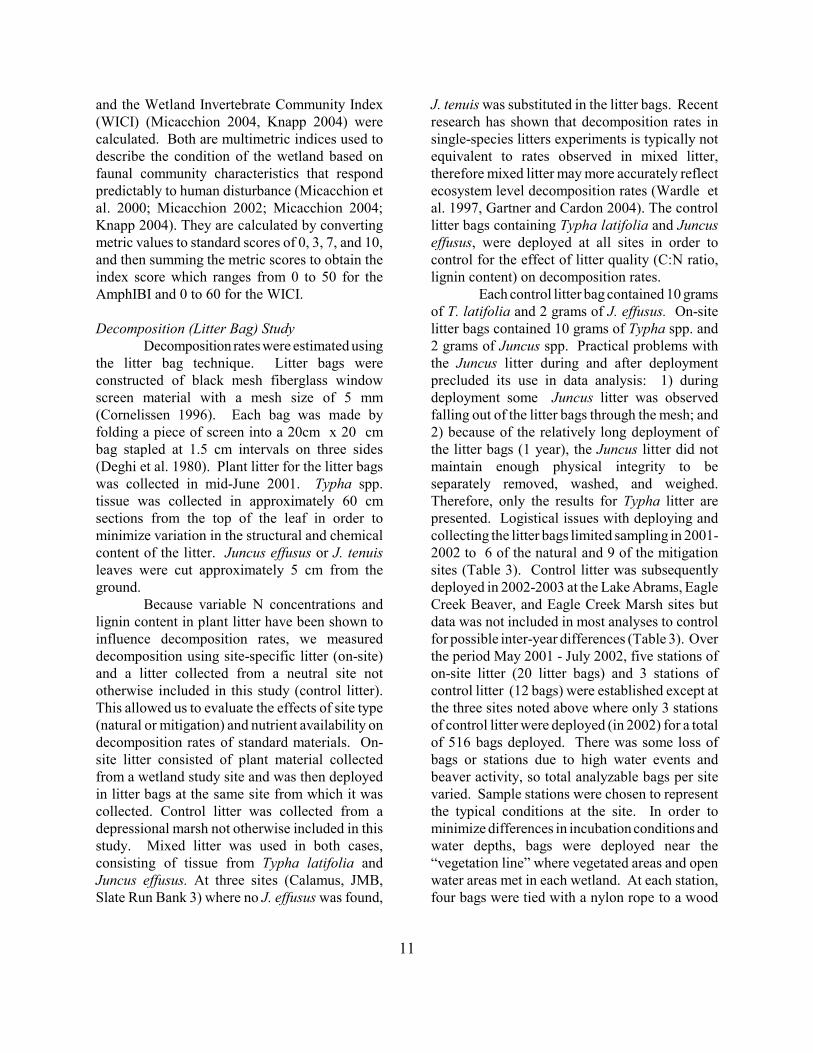
Decomposition (Litter Bag) Study Decomposition rates were estimated using

the litter bag technique. Litter bags wereconstructed of black mesh fiberglass windowscreen material with a mesh size of 5 mm(Cornelissen 1996). Each bag was made byfolding a piece of screen into a 20cm x 20 cmbag stapled at 1.5 cm intervals on three sides(Deghi et al. 1980). Plant litter for the litter bagswas collected in mid-June 2001. Typha spp.tissue was collected in approximately 60 cmsections from the top of the leaf in order tominimize variation in the structural and chemicalcontent of the litter. Juncus effusus or J. tenuisleaves were cut approximately 5 cm from theground.

Because variable N concentrations andlignin content in plant litter have been shown toinfluence decomposition rates, we measureddecomposition using site-specific litter (on-site)and a litter collected from a neutral site nototherwise included in this study (control litter).This allowed us to evaluate the effects of site type(natural or mitigation) and nutrient availability ondecomposition rates of standard materials. On-site litter consisted of plant material collectedfrom a wetland study site and was then deployedin litter bags at the same site from which it wascollected. Control litter was collected from adepressional marsh not otherwise included in thisstudy. Mixed litter was used in both cases,consisting of tissue from Typha latifolia andJuncus effusus. At three sites (Calamus, JMB,Slate Run Bank 3) where no J. effusus was found,

J. tenuis was substituted in the litter bags. Recentresearch has shown that decomposition rates insingle-species litters experiments is typically notequivalent to rates observed in mixed litter,therefore mixed litter may more accurately reflectecosystem level decomposition rates (Wardle etal. 1997, Gartner and Cardon 2004). The controllitter bags containing Typha latifolia and Juncuseffusus, were deployed at all sites in order tocontrol for the effect of litter quality (C:N ratio,lignin content) on decomposition rates.

Each control litter bag contained 10 gramsof T. latifolia and 2 grams of J. effusus. On-sitelitter bags contained 10 grams of Typha spp. and2 grams of Juncus spp. Practical problems withthe Juncus litter during and after deploymentprecluded its use in data analysis: 1) duringdeployment some Juncus litter was observedfalling out of the litter bags through the mesh; and2) because of the relatively long deployment ofthe litter bags (1 year), the Juncus litter did notmaintain enough physical integrity to beseparately removed, washed, and weighed.Therefore, only the results for Typha litter arepresented. Logistical issues with deploying andcollecting the litter bags limited sampling in 2001-2002 to 6 of the natural and 9 of the mitigationsites (Table 3). Control litter was subsequentlydeployed in 2002-2003 at the Lake Abrams, EagleCreek Beaver, and Eagle Creek Marsh sites butdata was not included in most analyses to controlfor possible inter-year differences (Table 3). Overthe period May 2001 - July 2002, five stations ofon-site litter (20 litter bags) and 3 stations ofcontrol litter (12 bags) were established except atthe three sites noted above where only 3 stationsof control litter were deployed (in 2002) for a totalof 516 bags deployed. There was some loss ofbags or stations due to high water events andbeaver activity, so total analyzable bags per sitevaried. Sample stations were chosen to representthe typical conditions at the site. In order tominimize differences in incubation conditions andwater depths, bags were deployed near the“vegetation line” where vegetated areas and openwater areas met in each wetland. At each station,four bags were tied with a nylon rope to a wood

12

stake to prevent movement of the bags. At each collection period, replicate bags

were retrieved from each site (for a total of 5 on-site bags and 3 control bags) and stored on ice fortransport. At the lab, litter remaining in each bagwas removed, briefly washed to remove dirt anddebris, separated by species (Typha and Juncus),and oven dried at 90°C to a constant weight. Theplant litter used in the litter bags was analyzed fornitrogen, phosphorus, calcium, magnesium, andpotassium content prior to deployment. These arereferred to as initial litter nutrient concentrations.Nutrient concentrations were also determined fora total of four on-site plant litter samples (2Typha, 2 Juncus), and three control plant samples(2 Typha, 1 Juncus) from each site. Each timelitter bags were collected from the field, threesamples of on-site litter and 2 of control litterfrom each site were selected at random foranalysis of the same parameters.

Litter samples were analyzed usingstandard methods (AOAC 1990). Followingmicrowave nitric acid digestion, elementalanalysis (except for %N) was done usingInductively Coupled Plasma Spectroscopy(Method 985.01, AOAC 1990 ). Nitrogen content(%) was determined using the Dumas Methodusing a LECO FP-428 Nitrogen Analyzer(Method 968.06 AOAC 1990). Litter sampleanalysis was done at Midwest Laboratories, Inc.,Omaha, Nebraska.

After each collection period, the percentmass lost was calculated in order to determinehow much litter was lost during each period.These data were also plotted in terms of percentmass remaining in order to track decompositionover time. Decomposition rates were calculated bydetermining k, a standard measure ofdecomposition (Molles 1999). The k-value wasdetermined as follows:

M t = M o e (-kt)

where M t = mass of litter present at time t, Mo =initial of litter, t = time in days, and k = dailyrate of mass loss (Molles 1999). The duration(days) of each incubation period is shown in

Table 3. Incubation times vary slightly becausefield logistics precluded us from deploying orcollecting litter bags from all sites on the sameday.

By quantifying the nutrient concentrationin the decaying litter following each collectionperiod, we were able to determine if differencesexisted in the nutrient dynamics of natural andmitigation wetlands. Nitrogen immobilization wascalculated based on changes in litter Nconcentrations between each collection date(Windham and Ehrenfeld 2003).

Data AnalysisMinitab statistical software v. 12.0 and

StatView v. 5.0 were used for all analyses exceptmacroinvertebrate data analysis where Systat v.9.0 was used and for multivariate analyses(Detrended Correspondence Analysis (DCA),Principal Components Analysis (PCA), ClusterAnalysis) where PC-ORD was used (McCune andMefford 1999). Descriptive statistics, box andwhisker plots, regression analysis, analysis ofvariance, multiple comparison tests, and t testswere used. Detrended Correspondence Analysis(Hill and Gauch 1980; Gouch 1982) and ClusterAnalysis (Sneath and Sokol 1973) were used toevaluate species presence and relative abundancedata. Principal Components Analysis was used toevaluate IBI metric performance. For the DCA,Euclidean distance was calculated and rarespecies were down weighted. For ClusterAnalysis, Sorensen similarity and Ward’s linkagemethod were used.

RESULTS

HydrologySeveral hydrological parameters (Table 4)

were calculated using data collected from May 1to September 30, 2001 and from April 1 toSeptember 30, 2002 (records were more completein the 2002 growing season): including thepercentage of time that water remained in the rootzone (defined as the top 30 cm of soil); mean andmedian ground water levels (shown in centimetersbelow the ground surface); and, the maximum and

13

minimum water levels recorded at each site.Positive values indicate that ground water levelswere above the ground surface. A “flashiness”index was developed by averaging the absolutevalue of the differences between each groundwater measurement from the measurement justpreceding it (Table 5).

Natural wetlands had water in the rootzone ranging from 100 to 23 percent of the timewhile mitigation wetlands ranged from 96 to 0percent of the time. On average, water remainedin the root zone of natural wetlands 50.7% longerthan in mitigation wetlands, although thisdifference was not significant (p = 0.21). Meanground water levels ranged from -58.2 to 4.2 cmat the natural sites and -12.2 to -0.7 cm at themitigation wetlands. The mitigation wetlandswere generally “dryer” than the natural sites basedon measures of ground water. Maximum groundwater depths recorded by the wells (note this isoften the lowest reading the well can record, notnecessarily the lowest water level actuallyoccurring) was -88.3 cm for the natural wetlands(Lodi) and -106.4 cm for the mitigation sites(Trotwood). Minimum depths recorded were 33.1cm for the natural sites (Baker Swamp) and 11.7cm for the mitigation sites (Medallion No. 20).

Box and whisker plots were constructedto compare mean hydrological parameters for thenatural and mitigation wetlands in both years, andunpaired t-tests were used to test for differencesbetween means (Figures 5a and 5b). Water waspresent in the root zone for nearly twice as long inthe natural sites during the 2001 growing season,and this difference was significant (31.9 + 11.3percent for mitigation versus 63.9 + 9.4 percentfor natural; p = 0.04). Similar data werecollected in 2002 when water was present in theroot zone for 37.2 +12.1 and 66.0 + 7.0 percent ofthe time for mitigation and natural sites,respectively (p = 0.059). Mean depth to groundwater reflects this, averaging -53.8 + 11.1 cm inthe mitigation sites and -25.0 + 6.1 cm in thenatural sites in 2001 (p = 0.04), and -44.5 + 9.1and -25.4 + 4.9 in 2002 (p = 0.09).

A comparison of mean surface waterlevels, mean ground water levels, and the

percentage of time that ground water was in theroot zone (Figure 6), shows that natural andmitigation wetlands have significant hydrologicaldifferences. Mitigation wetlands had both deepersurface water and greater mean depth to groundwater, leaving a substantial unsaturated zone inthe upper soil for most of the growing season.This indicates a ‘disconnect’ between surface andground waters at the mitigation wetlands. Theheavy clay soils that characterize many of themitigation sites appear to limit the verticalmovement of water through the root zone, makingthe mitigation sites less hydrologically dynamic(see Table 9) for data on bulk density and percentsolids). The combination of deeper surface waterand drier soils (lower ground water) hasimplications for plant growth (water available forroot uptake) and biogeochemical processes suchas denitrification because the relative lack ofwater flux also limits the movement ofcompounds such as nitrate and dissolved organiccarbon needed by microbial communities. Thefunctional consequences of this are not known,but appear to create substantial differences in thebiogeochemistry of the two types of wetlands.

Hydrologic “flashiness” ranged from 1.0to 4.6; maximum single day change in water levelsranged from 16.0 cm to 79.2 cm (Table 5). EagleCreek Beaver had the lowest score due to themoderating influence of ground water on its dailywater levels; Lake Abrams, Lodi North, andTrotwood had the highest scores due to highstormwater inputs (Table 5). Sites with verystrong depressional hydrology (vertical hydrologicpathway driven by precipitation andevapotranspiration had flashiness scores of 1.0 to~2.0. Index scores of between 2 and 3 occurred atsites with some riverine association or small tomoderate stormwater inputs. Scores greater than3 were indicative of high stormwater inputsdisrupting the natural hydroperiod.

Hydrographs for all wetlands included inthis study were constructed (Figures 7 to 12). Ingeneral, ground water levels in the mitigation sitesdeclined earlier in the growing season than in thenatural sites (for those sites that did dry down),and had less daily variation in water levels.

14

Several hydrologic signatures can be recognizedin each group. In the natural sites there are twobasic patterns evident, one in which ground wateris a significant influence that maintains relativelyconstant water levels throughout the growingseason (i.e. permanently inundated/saturated sitesincluding Baker Swamp, Ballfield, Eagle CreekBeaver), and one in which there is a dry downthrough the early summer to some low level laterin the growing season. Seasonally floodedwetlands include Calamus, Dever, Eagle CreekMarsh, Lake Abrams, Lodi, and Rickenbacker.Seasonally flooded wetlands are common in Ohiowith standing water in the spring and earlysummer and dry soils in the late summer and earlyautumn, however in nearly all cases, ground waterlevels are within the upper portion of the soil thatis measurable by the well (greater than ~ 80cm).Only Rickenbacker and Eagle Creek Marsh showlong periods (> 1 week) where water levels fellbelow the bottom of the well.

Several sites (Eagle Creek Marsh,Rickenbacker) show a rewetting during July, 2001in response to rainfall events. Both sites began todry down again almost immediately, withRickenbacker only taking a few days for waterlevels to drop again below the level of the well.For all sites, water levels at the well locations(near the edge of the wetlands) were very nearlyat or above the ground surface early in thegrowing season.

There are three basic hydrologicsignatures observed for the mitigation wetlands(Table 5, Figures 7 to 12): permanently flooded,seasonally flooded, and “dry,” where groundwater levels are very low (defined here aspermanently below the root zone at 30cm) andremain so throughout the growing season. Themajority of the mitigation sites show a seasonallyflooded hydrologic signature (Big Island Area D,JMB, New Albany HS, Prairie Lane, Slate RunBank SE). However, unlike the natural wetlands,these still underwent dry down to the extent thatground water levels drop below the level of thewell (noted by a flat line where levels are lowest).The dry down curves are generally steeper for themitigation sites, resulting in water levels that

bottom out by June. In some cases, mid-summerprecipitation caused ground water levels to rise; inthe case of New Albany water levels remain highfor the remainder of the growing season, for theothers (e.g., Prairie Lane) water levels rise andthen fall again below the bottom of the well. Bycontrast, Medallion and Pizzutti have apermanently flooded ground water signaturewhere ground water levels remain high throughoutthe growing season. These sites had surface waterpresent throughout the growing season as well.

Bluebird and Trotwood have what can beconsidered a “dry” ground water signature, onewhere ground water levels are low throughout thegrowing season. At Trotwood this “dry” groundwater signature occurred even though the site ispermanently inundated year round with surfacewater. Trotwood was also the flashiest of themitigation sites (Table 5) due to massivestormwater inputs from surrounding shoppingcenters and suburban development. The surfaceand ground water at this site appear to becompletely disconnected. The hydrograph forBluebird shows more fluctuation over time, butthe soils remain unsaturated above 50 cm for theduration of the growing season.

Water Chemistry Water chemistry parameters for the

natural and mitigation wetlands revealed nosignificant differences in the availability ofnutrients (e.g. ammonia, total P, TKN), cations(Ca2+, Mg2+), or physical measurements (pH, TSS)(Table 6). Mean concentrations of these para-meters are typical of those found in freshwatermarshes (Mitsch and Gosselink 2000), althoughfor several parameters, average concentrationswere higher in the natural sites including TotalOrganic Carbon (TOC).

Water chemistry of a larger referencewetland data set was also examined in order toplace the sites included in this study in the contextof wetland types across Ohio. Water chemistryparameters are summarized in Table 7. Mitiga-tion wetlands have median values in the range ofconcentrations typical of natural depressional andriverine marshes for TOC, Ca, Fe, Mg, Chloride,

15

Ammonia, and total P (Table 7); however, totalsuspended solids (TSS) at mitigation wetlandswas high (33 mg l-1) and similar to values found inriverine mainstem marshes (47 mg l-1), forests (25mg l-1), and shrub swamps (38 mg l-1), riverineheadwater marshes (27 mg l-1), and coastalmarshes (77 mg l-1) (Table 7).

Comparing water chemistry of mitigationsites to other wetlands types reveals differencesfor other parameters. As expected bogs havehigher median values for TOC (45-59% higher),as did Lake Plains sand prairies (35%), vernalpools (17-29%), wet woods (39%), and mainstemforests and shrub swamps (25% and 38%) (Table7). Median Ca concentrations are lower at bogs(3-16 mg l-1) and much higher at ground waterdriven systems like fens (up to 59 mg l-1) andcoastal marshes (58 mg l-1) (Table 7). Chloride,Ammonia, and P concentrations can increasesubstantially at natural wetlands receiving stormwater inputs. The 75th percentile for theseparameters at natural marshes can be as a high as176 mg l-1, 0.24 mg l-1 and 0.51 mg l-1,respectively (Table 7).

SoilsOf the 21 common soil parameters shown

in Table 8, 19 parameters were significantlydifferent (p < 0.10) when average values ofnatural and mitigation wetlands were compared.Average concentrations of organic carbon(%OC), %N, and plant available P (µg P g-1 soil)were 6.2 times, 4.6 times and 1.6 times higher,respectively, in the natural sites compared to themitigation ones. The average nitrogen content (as%N) in natural wetlands was 1.12% compared toa very low 0.24% in the mitigation systems (Table8; Figure 13). Organic carbon averaged 15.1% innatural wetlands compared to 2.45% in mitigationsystems, and the average concentration of plantavailable P in the natural wetlands was 11.96 µgg-1 and 43.4 µg g-1 com-pared to 7.38 µg g-1 and30.0 µg g-1 in the mitigation systems for weak andstrong Bray analyses, respectively. Total P, whichis a measure of all P held in the soil (includingthat which is not readily available), showed asimilar pattern with levels of 1156 µg g-1 in the

natural soils, nearly twice as high as in mitigationsoils, which averaged 669 µg g-1. Soil ammoniawas more than three times higher in natural soils,averaging 62.4 µg g-1 and 20.5 µg g-1 in thenatural and mitigation sites.

Exchangeable cations provide animportant index of fertility and plant growth.Total and exchangeable K and Mg were higher inmitigation wetlands; total Ca was higher inmitigation wetlands but the proportion ofexchangeable Ca was lower. The ratio of Ca2+ toMg2+ differed in the two groups, ranging from 6.7in the natural to 4.4 in the mitigation sites,indicating a relative lack of available Ca2+.Overall, cation exchange capacity was nearly 1.5times higher at the natural wetlands.

Mean values for soil bulk density,%solids, particle size of midrange (2 - 50 µm)and large (>50 µm) particles, and pH betweennatural and mitigation wetlands were alsosignificantly different (Figure 14). The pH ofnatural sites was significantly lower than themitigation sites, averaging 5.58 and 6.19,respectively. The average bulk density of naturalwetland soil was 0.62 g cm-3 compared to 1.75 gcm-3 in the mitigation wetlands. Values for percentsolids also differ accordingly, averaging 42.5% innatural and 73.5% in mitigation sites. Averagesize of soil particles was lower (31.5%) formidrange particles and higher for larger particles(53.8%) for natural wetlands than for mitigationwetlands (41.9% midrange, 39.7% large). Thesemeasures quantify the extremely heavy soils foundin the mitigation sites that may lead to reducedroot growth and limit carbon accumulation(Tables 8 and 9). In a cluster analysis based onthe average nitrogen and carbon content of bothnatural and mitigation wetlands 9 of the 10mitigation wetlands grouped together, i.e.mitigation wetlands had soil characteristics uniquefrom the natural sites (Figure 15). The distinctseparation of the two groups indicates that thereare two ecologically distinct wetland populationsbased on soils.

Soil chemistry of a larger referencewetland data set was also examined in order toplace the sites included in this study in the context

16

of wetland types across Ohio. These values aresummarized in Table 10. Median values for Al,Ca, Fe, Mg, K, and P total were similar to medianconcentrations and ranges found in other naturalmarshes. Median ammonia concentrations atmitigation wetlands was at the lower end ofnatural wetland values (24 mg kg-1) and was muchlower than depressional marshes (39 mg kg-1),mainstem marshes (54 mg kg-1), or headwatermarshes (77 mg kg-1), and was more similar tonutrient poor bogs and fens (Table 10). Strikingdifferences were observed when comparing%solids and TOC of soils in mitigation wetlandsto all natural wetlands: mitigation wetlands hadthe highest median %solids (73.3%) and lowestmedian TOC (2.0%) of all soil samples analyzed(Table 10).

VegetationBecause individual plant species are

differentially sensitive to environmental stressors,and vegetation is always present in wetlands, it isthe most common assemblage used to assess thecondition and development of wetland ecosystems(Fennessy et al. 2002; Cronk and Fennessy 2002).In order to determine if differences between thevegetation communities of natural and mitigationwetlands existed, plant-based attributes includingthe Vegetation IBI and its component metrics(Mack 2004b), plant species richness, the FQAI,and the level of aboveground biomass productionwere calculated for each site (Tables 11 and 12).

Scores for the VIBI–Emergent (Mack2004b) were calculated for all sites. Scores fornatural sites ranged from 9 to 82, reflecting thefact that the natural wetlands were chosen along agradient of human disturbance (Table 11). Thisrange encompasses nearly the entire range ofscores for emergent wetlands in Ohio. Scores formitigation wetlands were much more consistent,ranging from 16 to 50. This compression ofscores is due in part to the fact that the communitycomposition of the mitigation sites is similar, witha dominance of ubiquitous, tolerant species.Mean VIBI scores were more than twice as high atnatural as for mitigation sites, and this differenceis highly significant (p = 0.005) (Table 12).

There was no significant difference between thespecies richness of natural and mitigation sites, anaverage of 31.0 species were recorded in the plotsat natural sites while an average of 25.6 werefound in the mitigation sites (p = 0.22) (Table 12).

In contrast FQAI scores were significantlydifferent in the two wetland populations, with anaverage score of 21.6 for the natural sites and 14.2for the mitigation sites (p = 0.004) (Table 12).The range of FQAI scores in the natural wetlandswas 15.8 to 31.0 (reflecting the humandisturbance gradient), whereas scores for themitigation wetlands ranged from 8.8 to 18.1.Despite the fact that the natural sites span agradient of disturbance, the range of scores for thetwo populations overlaps only marginally(between 15.8 and 18.1) (Table 11).

Aboveground biomass, a measure ofwetland primary productivity, was significantlyhigher in natural sites which produced an average34.7 g 0.1 m-2 (equivalent to 347 g m-2) whilemitigation sites produced an average of 20.9 g 0.1m-2 (209 g m-2) (Table 12). Thus production rateswere an average of 1.7 times higher in naturalwetlands (unpaired t-test, p = 0.04). However,when average standing biomass of mitigationwetlands was compared to natural wetlands inthree disturbance categories, mitigation wetlandshad standing biomass similar to least disturbednatural sites (Figure 22b). This was due to largeareas of unvegetated water or bare ground or soilnutrient limitations at many of the mitigationwetlands.

Finally, all vascular plants recorded ineach wetland were categorized according to theirwetland indicator status, a measure of theirfidelity to wetland habitats (Reed 1988). Naturalwetlands contained significantly greater numbersof obligate species (those found in wetlands 99%of the time), and had higher means of FACW andFAC species. This may in part be due to therelatively dry soils found at the mitigation sites(Figure 16).

The VIBI has been shown to respondpredictably to human disturbance and hasundergone two major evaluations withindependent data sets to validate its usefulness as

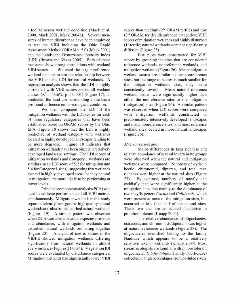
17

a tool to assess wetland condition (Mack et al.2000, Mack 2001, Mack 2004b). Several mea-sures of human disturbance have been employedto test the VIBI including the Ohio RapidAssessment Method (ORAM v. 5.0) (Mack 2001)and the Landscape Disturbance Intensity Index(LDI) (Brown and Vivas 2005). Both of thesemeasures show strong correlations with wetlandVIBI scores. We used the larger referencewetland data set to test the relationship betweenthe VIBI and the LDI for natural wetlands. Aregression analysis shows that the LDI is highlycorrelated with VIBI scores across all wetlandclasses (R2 = 43.6%, p < 0.001) (Figure 17); aspredicted, the land use surrounding a site has aprofound influence on its ecological condition.

We then compared the LDI of themitigation wetlands with the LDI scores for eachof three regulatory categories that have beenestablished based on ORAM scores by the OhioEPA. Figure 18 shows that the LDI is highlypredictive of wetland category with wetlandslocated in highly developed landscapes tending tobe more degraded. Figure 18 indicates thatmitigation wetlands have been placed in relativelydeveloped landscape settings. The LDI scores ofmitigation wetlands and Category 1 wetlands aresimilar (mean LDI score of 5.2 for mitigation and5.4 for Category 1 sites), suggesting that wetlandslocated in highly developed areas, be they naturalor mitigation, are more likely to be performing atlower levels..

Principal components analysis (PCA) wasused to evaluate performance of all VIBI metricssimultaneously. Mitigation wetlands in this studyseparated clearly from good to high quality naturalwetlands and also from disturbed natural wetlands(Figure 19). A similar pattern was observedwhen DCA was used to evaluate species presenceand abundance, with mitigation wetlands anddisturbed natural wetlands ordinating together(Figure 20). Analysis of metric values in theVIBI-E showed mitigation wetlands differingsignificantly from natural wetlands in almostevery instance (Figures 21 to 24). Vegetation IBIscores were evaluated by disturbance categories.Mitigation wetlands had significantly lower VIBI

scores than medium (2nd ORAM tertile) and low(3rd ORAM tertile) disturbance categories; VIBIscores of mitigation wetlands and highly disturbed(1st tertile) natural wetlands were not significantlydifferent (Figure 25).

Box plots were constructed for VIBIscores by grouping the sites that are consideredreference wetlands, nonreference wetlands, andmitigation wetlands (Figure 26). Mean mitigationwetland scores are similar to the nonreferencesites, but the range of scores is much smaller forthe mitigation wetlands (i.e., they scoreconsistently lower). Mean natural referencewetland scores were significantly higher thaneither the nonreference sites or the mitigation(mitigation) sites (Figure 26). A similar patternwas observed when LDI scores were comparedwith mitigation wetlands constructed inpredominately intensively developed landscapesand many nonreference sites, and most referencewetland sites located in more natural landscapes(Figure 26).

MacroinvertebratesMajor differences in taxa richness and

relative abundance of several invertebrate groupswere observed when the natural and mitigationwetlands were compared. Numbers of dytiscidbeetle, chironomid, dipteran, and total taxarichness were higher at the natural sites (Figure27). By contrast, numbers of mayfly andcaddisfly taxa were significantly higher at themitigation sites due mainly to the dominance oftwo mayfly genera Caenis and Callibaetis, whichwere present at most of the mitigation sites, butoccurred at less than half of the natural sites.These two taxa are considered facultative topollution tolerant (Knapp 2004).

The relative abundance of oligochaetes,ostracods, and chironomids/dipterans was higherat natural reference wetlands (Figure 28). Theoligochaetes identified belong to the familyNaididae which appears to be a relativelysensitive taxa in wetlands (Knapp 2004). Moststream ecologists are familiar with a more tolerantoligochaete, Tubifex tubifex (Family Tubificidae)collected in high percentages from polluted rivers

18

and streams. Ostracods also appear to be relativelysensitive taxa in wetlands. Some varieties ofostracods are sensitive to herbicides andpesticides (Thorp and Covich 2001).

Relative abundance of tolerant beetles,corixids, and tolerant snails were higher in themitigation sites. The adult beetle genera,Haliplus, Peltodytes, and Tropisternus areherbivores. They are commonly found in densemats of aquatic vegetation or algae mats. At thenatural sites, there were higher numbers ofdytiscid beetle taxa. The adult dytiscid beetles arepredacious. Corixidae abundance was higher atthe mitigation sites, especially the generaRamphocorixa, Sigrara, and Trichocorixa. In thereference sites only the corixid genusHesperocorixa was collected in moderatenumbers. The tolerant snail genera Physella andGyraulus were more abundant at the mitigationsites.

Box plots of a wetland invertebratecommunity index (WICI) scores for mitigation,nonreference, and reference sites are shown inFigure 29. Mitigation sites had significantlylower WICI scores (mean of 13) due to highrelative abundance of tolerant taxa (with fewersensitive taxa) than nonreference (mean of 27)and reference (43) wetlands. The observed macro-invertebrate trophic structure differed substan-tially in the two types of wetlands (Figure 30).

AmphibiansAmphibian community data were used to

calculate various faunal community attributes andindicators including the Amphibian Index ofBiotic Integrity (AmphIBI) score (Micacchion2004). Ordinations of the species composition ofnatural and constructed wetlands were examined.For the amphibian analysis information from alarger natural reference wetland data set was alsoincluded.

Nine of the 10 mitigation wetlands hadAmphIBI scores of 0 (mean score = 0.3). SlateRun Bank SE was the only mitigation site with ascore greater than 0 (AmphIBI score = 3) due tothe presence of tiger salamanders (Ambystomatigrinum). This site was built at the edge of an

existing forested area that had a breedingpopulation of tiger salamanders. The 9 naturalemergent wetlands had AmphIBI scores thatranged from 0 to 17 (mean score = 6.55). Thedifferences in mean AmphIBI scores betweennatural and mitigation wetlands were significant(p < 0.05).

Data collected between 1996-2002 in alarger reference wetland data set (n = 101) wasincluded in the ordination with the 10 mitigationwetlands sampled for this study. Mean AmphIBIscores between reference (least-impacted),nonreference (moderate to severe disturbance)natural wetlands and the mitigation wetlands weresignificantly different (Figure 31). A PCA ofindividual AmphIBI metrics showed mitigationsites in a very tight cluster surrounded by othernatural emergent wetlands (Figure 32). Bothmitigation wetlands and natural emergentwetlands were separated from wetland forests andshrub swamps (Figure 32).

Ordination of species presence andrelative abundance using DCA revealed cleardifferences between natural emergent, forest, andshrub wetlands and the mitigation wetlandsstudied here (Figure 33). Most good to highquality shrub and forest wetlands groupedtogether on the far right side of the graph. Themitigation sites formed a group with some naturalemergent wetlands and a few of the lower qualityshrub and forested wetlands (Figure 33). Thesegroupings were due to the presence andabundance of sensitive, forest dependentamphibian species like wood frog (Ranasylvatica) and spotted salamander (Ambystomamaculatum) at the good to high quality shrub andforest sites (Figure 33).

When only the mitigation and naturalemergent sites included in this study wereordinated, there was no strong separation ofnatural and mitigation sites. Rather, the sitesordinate more on the basis of the permanency ofhydrology and the corresponding presence ofpredatory fish (data not shown). Those wetlandswith the more permanent surface water andpresence of predatory fish cluster in the upperright portion of the graph and those with seasonal

19

hydrology and no predatory fish cluster in lowerleft portion of the graph. Two sites with high toad(Bufo spp.)5 dominance (Prairie Lane, Big IslandArea D) are far removed from the other sites inthe upper left corner of the graph (Figure 34).

DecompositionAfter the first incubation period (~37

days), a significant difference was found in Typhadecomposition rates in which natural sites lost anaverage of 4.53 g (or 45.3%) of on-site litter fromeach bag and mitigation wetlands sites lost anaverage of 3.92 g (39.2%) (p = 0.067) (Tables 13and 14). The k-values calculated for the naturaland mitigation sites did not differ significantly,but natural wetlands had a faster average rate ofdecay as compared to mitigation wetlands (0.0167and 0.0139) (Tables 13 and 14).

Initial difference in the decompositionrates persisted throughout the study. Mass lostwas higher at natural than mitigation sites at thesecond pick up (~87 days), with a mean loss of5.86 g and 4.49 g, respectively (p = 0.05). At thethird pick up, mean differences were 6.26 gcompared to 5.11 g lost (p = 0.05). Figure 35shows this data graphically as the percent massremaining at each collection period. The dataindicate that there are distinct differences in boththe short-term (approximately 1 month) andlonger term (approximately 1 year) decayprocesses of the on-site litter between natural andmitigation wetlands.

We used control litter of uniform C:Nratio to help isolate differences in decompositionrates and short term nutrient flux in natural andmitigation wetlands other than differencesresulting from the chemical composition of theplant material itself. As with on-site litter, meandecomposition rates for control litter were fasterin natural wetlands. Differences were significantat the second and third pick-up (Tables 15 and16). At the third pick-up an average of 7.14 g (or71.4%) had been lost from natural sites, while

only 5.34 g (53.4%) had been lost at themitigation sites. Thus the natural sites lost nearly1.3 times more litter than the mitigation sitesindicating significantly higher levels of microbialactivity and higher rates of nutrient flux (see nextsection). K values show a similar pattern withhighly significant differences at the third-pick up.At the end of nearly one year, natural sites had29% of the original litter remaining whilemitigation sites had nearly half (47%) of theprevious year’s litter left in the system. Bio-geochemical transformations appear to behappening much more slowly in the mitigationwetlands (Figure 36).

Plant Litter Nutrient AnalysisInitial concentrations of both nitrogen and

phosphorus in on-site plant litter was significantlyhigher in natural wetlands. Litter nitrogen levelsaveraged 0.4 percent higher at natural sites (p =0.09) (Figure 37). The initial phosphorus contentat natural sites averaged 0.29 µg P g-1 litter whilemitigation sites had a mean concentration of 0.25µg P g-1 litter (p = 0.01) (Figure 38). Plant nutri-ent concentrations show a general pattern ofdecline due to initial leaching, followed by anincrease at the second and third measurements asmicrobial colonization of the litter progresses(Figures 37 and 38). Despite differences in initialconcentrations, N concentrations at the time offirst pick-up (~37 d) were essentially equal (2.7 %N and 2.6 % N by weight, respectively (Figure37), indicating that N was leached more rapidly atthe natural sites. Leaching is common in the earlystages of decomposition and represents a flush ofnutrients that is then available for microbialgrowth and plant uptake. The amount of Nleached at the mitigation sites amounted to lessthan half that lost at the natural wetlands. At thesecond pickup (87 d), litter N concentrations hadincreased rapidly in the natural wetlands(increasing by nearly 20%) while N levels stayedconstant in the mitigation sites. This resulted insignificantly higher mean concentrations of 3.18%, compared to 2.66 % in the mitigation sites (p= 0.07). N concentrations converged slightly asdecomposition progressed as levels increased

5 American toad (Bufo americanus)and Fowlers toad (Bufo fowleri) tadpoles cannot bedifferentiated and results are aggregated.

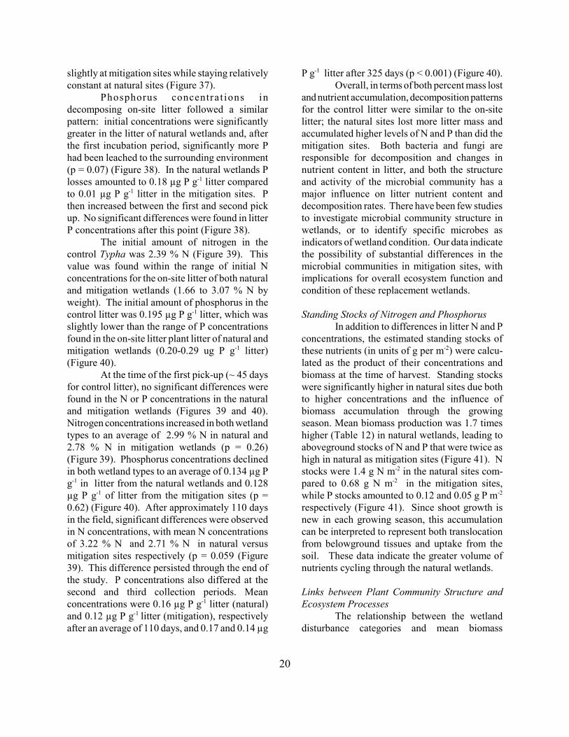
20

slightly at mitigation sites while staying relativelyconstant at natural sites (Figure 37).

Phosphorus concentrat ions indecomposing on-site litter followed a similarpattern: initial concentrations were significantlygreater in the litter of natural wetlands and, afterthe first incubation period, significantly more Phad been leached to the surrounding environment(p = 0.07) (Figure 38). In the natural wetlands Plosses amounted to 0.18 µg P g-1 litter comparedto 0.01 µg P g-1 litter in the mitigation sites. Pthen increased between the first and second pickup. No significant differences were found in litterP concentrations after this point (Figure 38).

The initial amount of nitrogen in thecontrol Typha was 2.39 % N (Figure 39). Thisvalue was found within the range of initial Nconcentrations for the on-site litter of both naturaland mitigation wetlands (1.66 to 3.07 % N byweight). The initial amount of phosphorus in thecontrol litter was 0.195 µg P g-1 litter, which wasslightly lower than the range of P concentrationsfound in the on-site litter plant litter of natural andmitigation wetlands (0.20-0.29 ug P g-1 litter)(Figure 40).

At the time of the first pick-up (~ 45 daysfor control litter), no significant differences werefound in the N or P concentrations in the naturaland mitigation wetlands (Figures 39 and 40).Nitrogen concentrations increased in both wetlandtypes to an average of 2.99 % N in natural and2.78 % N in mitigation wetlands (p = 0.26)(Figure 39). Phosphorus concentrations declinedin both wetland types to an average of 0.134 µg Pg-1 in litter from the natural wetlands and 0.128µg P g-1 of litter from the mitigation sites (p =0.62) (Figure 40). After approximately 110 daysin the field, significant differences were observedin N concentrations, with mean N concentrationsof 3.22 % N and 2.71 % N in natural versusmitigation sites respectively (p = 0.059 (Figure39). This difference persisted through the end ofthe study. P concentrations also differed at thesecond and third collection periods. Meanconcentrations were 0.16 µg P g-1 litter (natural)and 0.12 µg P g-1 litter (mitigation), respectivelyafter an average of 110 days, and 0.17 and 0.14 µg

P g-1 litter after 325 days (p < 0.001) (Figure 40).Overall, in terms of both percent mass lost

and nutrient accumulation, decomposition patternsfor the control litter were similar to the on-sitelitter; the natural sites lost more litter mass andaccumulated higher levels of N and P than did themitigation sites. Both bacteria and fungi areresponsible for decomposition and changes innutrient content in litter, and both the structureand activity of the microbial community has amajor influence on litter nutrient content anddecomposition rates. There have been few studiesto investigate microbial community structure inwetlands, or to identify specific microbes asindicators of wetland condition. Our data indicatethe possibility of substantial differences in themicrobial communities in mitigation sites, withimplications for overall ecosystem function andcondition of these replacement wetlands.

Standing Stocks of Nitrogen and PhosphorusIn addition to differences in litter N and P

concentrations, the estimated standing stocks ofthese nutrients (in units of g per m-2) were calcu-lated as the product of their concentrations andbiomass at the time of harvest. Standing stockswere significantly higher in natural sites due bothto higher concentrations and the influence ofbiomass accumulation through the growingseason. Mean biomass production was 1.7 timeshigher (Table 12) in natural wetlands, leading toaboveground stocks of N and P that were twice ashigh in natural as mitigation sites (Figure 41). Nstocks were 1.4 g N m-2 in the natural sites com-pared to 0.68 g N m-2 in the mitigation sites,while P stocks amounted to 0.12 and 0.05 g P m-2

respectively (Figure 41). Since shoot growth isnew in each growing season, this accumulationcan be interpreted to represent both translocationfrom belowground tissues and uptake from thesoil. These data indicate the greater volume ofnutrients cycling through the natural wetlands.

Links between Plant Community Structure andEcosystem Processes

The relationship between the wetlanddisturbance categories and mean biomass

21

production (g 0.1 m-2) was investigated using thelarger data set available for emergent marshes inOhio (Figure 42). Biomass production is nega-tively correlated with VIBI scores (by disturbancecategory), supporting our hypothesis that pro-ductivity will increase as VIBI scores decline.This is an ecologically predicable relationship forwetlands since as a site becomes disturbed byhuman activities, invasive, highly productivespecies tend to become dominant. Because theVIBI integrates information about the relativetolerance levels, species composition and, as oneof its metrics, biomass production, these twomeasures are not completely independent. Inorder to further explore this relationship, aregression of biomass production versus FQAIscores was plotted for the sites included in thisstudy (Figure 43). The slopes of the regressionlines for the two wetland populations were verydifferent so each is plotted individually. Bothshow the same trend: biomass production de-clines as FQAI scores increase (again an eco-logically predictable relationship (Keddy 1993),however the slope of the line for the mitigationsites is much steeper than for the natural wetlands,and intercepts the x-axis at a lower value. Atnearly all points along the line, for sites with thesame FQAI score, the models predict that thenatural wetlands will have greater biomass.

A box plot showing the mean decomposi-tion rates for wetlands by disturbance categoryshows a trend (insufficient data for statisticaltesting by category) of increasing rates as afunction of ecological condition (Figure 44). Inorder to test this relationship more fully, and totest decomposition rates as a potential indicator ofcondition, a more extensive data set will benecessary. As described above, mean rates werelowest overall for the mitigation sites anddisturbed natural wetlands. This lends support tothe hypothesis that impaired wetlands have slowerdecomposition rates.

The soil and water data presented earlierin this report demonstrate the low levels oforganic carbon contained in the mitigationwetlands. Wetland food webs tend to bedominated by heterotrophs, making the

availability of organic carbon an important driverof ecosystem processes. Low organic carbonlevels can limit the activity of decomposers(heterotrophic microbes and invertebrates) andlead to lower rates of decomposition in thesystem. In order to more explore this link, weperformed regression analyses of decompositionrates across the range of organic matter availablein the natural wetlands (since carbon levels wereconsistently low in the mitigation sites). Bothwater and soil organic carbon are highlycorrelated with decomposition rates (Figures 45and 46).

DISCUSSION

The biological and biogeochemicalcharacteristics of the natural and mitigationwetlands in this study were substantially different.The natural wetlands had faster rates ofdecomposition, higher IBI scores, biomassproduction, soil nutrient concentrations, and plantlitter nutrient concentrations. Significantdifferences in hydrological patterns were alsoobserved.

HydrologyThe hydrodynamics of the two groups of

wetlands were significantly different. Whileground water levels were significantly lower inthe mitigation sites, mean surface water levelswere higher. We predicted that mitigationwetlands would have higher ground water levelsdue to the presence of high, often permanent,surface water levels. Our data indicate ahydrological "disconnect" between the surfaceand ground water in the mitigation wetlandswhere soils in the root zone are “dry” even thoughthe site is inundated with large areas of openwater. For example, on June 6, 2001, the surfacewater depth was 90 cm at the edge of the pool atthe Bluebird mitigation wetland while the groundwater reading at this location was –22.4 cm. Thehigh bulk density of the soils is one probablecause of this hydrological disconnection. Heavy,non-porous soils prevent water movement throughthe soil. Soils in the mitigation wetlands appear to

22

be acting as a clay pan, keeping surface watersperched. This contributed to other hydrologicaldifferences such as the significantly shorterduration of water in the root zone at mitigationsites. This may present limitations to macrophytegrowth and reproduction since the majority ofvascular wetland plants obtain water and nutrientsthrough their roots.

Cole and Brooks (2000) studied twomitigation wetlands and found that surface waterwas present for longer periods than in two naturalsites; but they also report water in the root zonefor longer periods. They suggest that hydrologicaldifferences are the result of permit requirements.Mitigation wetlands usually have a hydrologicalstandard that must me met. In order to ensuremitigation wetlands achieve “wetland hydrology”they are often deliberately made overly deep as atype of insurance that water will be present (Coleand Brooks 2000). This results in "wetlands" thatare basically shallow ponds with distinct hydro-logical differences from typical natural wetlands.

Contrary to Cole and Brooks (2000), wefound that the depth to ground water was greaterand the duration of water in the root zone wassignificantly shorter in the mitigation sites.Improper hydrology will limit the successivedevelopment towards a more natural ecosystem(in terms of both vegetation and animalcommunities). Natural wetlands had higheraverage ground water levels during the growingseason and many of them experienced a dry downperiod in which very little or no surface water waspresent. Dry down periods are important for therejuvenation of the vegetation community by thedispersal and germination of seeds (Cronk andFennessy 2001). Wetlands that maintain perma-nently saturated conditions typically have lowerspecies diversity than those that have fluctuatingwater levels. A fluctuating hydroperiod also tendsto enhance productivity, organic matter accu-mulation, and nutrient cycling by creating a morespecies rich environment (Mitsch and Gosselink2000).

Soil The soil composition of the mitigation

wetlands were confirms the results of otherstudies: the soil constituents measured weremarkedly different from natural wetlands soils(Tables 9 and 10). Phosphorus, nitrogen, andcarbon were significantly lower in the mitigationsites. Low organic matter content and nutrientavailability have been shown to limit thedevelopment of wetland creation projects (Gibsonet al. 1994, Bishel-Machung 1996, Shaffer andErnst 1999, Stolt et al. 2000). Bishel-Machung etal. (1996) found that soil organic matter levels(SOM) in natural palustrine wetlands were 6.6%to 16.1% higher than in mitigation sites.Similarly, Shaffer and Ernst (1999) measuredSOM in 95 palustrine mitigation wetlands inPortland, Oregon and found that natural wetlandsoils contained an average of 59.1% more SOMthan mitigation sites. Stolt et al. (2000) found thatreference palustrine wetlands had 5 to 10 timesmore organic carbon compared to mitigationsystems. In our study, total carbon levels wereover 6 times higher in the natural sites. At 9 outof 10 of the mitigation sites, soil carbon(measured as both %OC, %OM) was lower thanthe minimum value found at any of the naturalsites. The New Albany HS mitigation wetland,which was built partially on the site of a formerwetland, was the only project with soils withorganic matter content approaching the minimumvalues of natural sites. The low levels of organicmatter are reflected in the bulk density and thepercent solids of the mitigation wetland soils.Average bulk density of the natural soils was 0.62g cm-3, significantly lower (p < 0.01) than the 1.75g cm-3 in the mitigation soils. Mean percent solidsvaried similarly.

The soils of the mitigation wetlandsincluded in our study were also deficient incritical plant nutrients including nitrogen,phosphorus and calcium. Nitrogen levels inmitigation and natural wetlands averaged 0.24%and 1.12% N, respectively. Bishel-Machung et al.(1996) and Stolt et al. (2000) also found higherlevels of total nitrogen in natural wetlands. Bishel-Machung et al. (1996) report median N values of0.29% in natural versus 0.11% in mitigationwetlands (p = 0.04). In our study, all 10

23

mitigation wetlands had lower nitrogen levels thanthe minimum concentration measured at any ofthe natural wetlands.

Several studies have documented Nlimitations in restored and created salt marshes(Zedler et al. 2001, Craft 2000, Langis et al.1991), but this has not been demonstrated infreshwater systems. Nitrogen availability has aninfluence on many ecosystem processes such asprimary production, biomass, diversity,reproductive potential, and plant tissue N content(Langis et al. 1991), therefore the low N suppliesin created sites may limit ecosystem function.Furthermore, there is no evidence that N levels areincreasing with time, nor do we understand thereasons for such low nutrient retention (Zedler etal. 2001). More studies are needed to determinethe mechanism(s) behind nitrogen and organicmatter accumulation in mitigation and naturalwetlands, and the time that might be required formitigation soils to develop characteristics ofnatural wetlands with and without any designinterventions, e.g. using donor soils from theimpact site or providing soil supplements tomitigation wetlands.

We investigated the relationship betweensite age and percent carbon and nitrogen, using aregression analysis. A positive relationship wouldprovide evidence that mitigation wetlands weredeveloping structural (and hence functional)equivalence. When the mitigation sites includedin this study were arrayed as a chronosequence,there was no relationship between site age and thecarbon or nitrogen content of the wetland soil(Figure 47). The soil data collected here does notsupport the assumption that soil indicators likecarbon or nitrogen are increasing over time.

The reasons behind low organic matteraccumulation (and low organic C content) in miti-gation sites has not been extensively studied.Bishel-Machung et al. (1996) were not able toexplain the differences between the organic matteraccumulation in natural and created wetlandswith measures such as landscape cover orvegetation. Interestingly, Cole et al. (2001) foundno relationship between biomass production andthe accumulation of SOM in created wetlands.

Shaffer and Ernst (1999) did find a relationshipbetween soil organic matter accumulation and theextent of inundation: wetlands that had lower soilorganic matter concentrations were saturated forlonger periods of time. This is an interestingrelationship because saturated conditionsgenerally slow the rates of decomposition andtherefore should increase the build-up of organicmatter.

The addition of soil amendments fromremnant or near-by wetlands is one method thatcould “jump start” the formation of nutrient richsoil (Brown and Bedford 1997). Stauffer andBrooks (1997) used additions of both leaf litterand soil organic matter in an attempt to acceleratethe development of newly created wetland plots.The researchers found that after two years, leaflitter plots contained an average of 8.2% organicmatter, which more closely resembles organicmatter levels found in of natural wetlands. Theuse of soil amendments appears to be a methodthat could be applied to nutrient-deficientmitigation wetlands.

One factor that appears to affect soilproperties is the method of wetland construction.Construction techniques have been shown tonegatively influence the structure anddevelopment of wetland soil. Mitigation marshesare often constructed by some or all of the soil’sA-horizon with heavy machinery. The A-horizonis typically high in organic matter and plantmaterials that are rich in nutrient content (Sposito1989). When the top layer of soil is removed theunderlying soil layer (B-horizon) is exposed. TheB-horizon often consists of thick clay materials(Sposito 1989). Stolt et al. (2000) for example,found that when the soil was excavated down tothe B-horizon, soil microrelief and plant diversitywere reduced. Many of the wetland sites in thisstudy were excavated down to the B-horizon andvisibly lacked any build up of organic sediments;time was not correlated with soil improvement.Better design and construction, along with arequirement that replacement wetlands are trulyrestoration projects (as opposed to createdwetlands built in upland locations) are needed toovercome this limitation.

24

Soil composition can serve as a measureof ecological integrity in order to gauge thedevelopment or progress of wetland mitigationprojects. The NRC (2000) recently described soilorganic matter content (or soil organic carbon) asthe “best” indicator of soil quality because itresponds to environmental disturbance andinfluences other functions within an ecosystem(NRC 2000). For example, soil characteristicshave been shown to influence the vegetationcomposition and the susceptibility of a wetland toinvasion by non-native species (Bishel-Machung1996, Shaffer and Ernst 1999, Brown and Bedford1997). Recent work has even equated soilcharacteristics, particularly organic carbon levelsto wetland condition and surrounding land use(Cohen et al. in press). For these reasons as wellas their ease of measurement, we propose thatboth SOM and N be used as indicators ofecosystem condition and as performancestandards.

VegetationThe vegetation-based bioassessment tools

that have been developed for use in monitoringand assessment provided clearly distinguishabledifferences in the two populations of wetlands.Mean VIBI scores were more than twice as highin the natural wetlands, despite the fact that thenatural wetlands were arranged along a gradientof disturbance. The Dever site was the lowestscoring natural wetland with a VIBI score of 9. Itis a remnant isolated wetland in a row crop field,receiving agricultural runoff and is dominated byTypha and other tolerant species common toagricultural wetlands. Big Island Area D was thehighest scoring mitigation site, with a VIBI of 50.This site is a 10.4 ha area that is part of a muchlarger mitigation bank (105 ha) that wasextensively planted and partially located on hydricsoils of a former wet prairie complex.

The composition of the communitiesvaried significantly. Mitigation sites consistentlydiffered from good to high quality naturalemergent marshes on most VIBI metrics (Figures21 to 24) and had similar average VIBI scores tohighly disturbed natural marshes (Figure 25).

Ordinations of plant species presence andabundance and individual metric performancesuggests that the mitigation wetlands studied areforming a distinct population of wetlands fromnatural wetlands. Mitigation wetlands had ahigher relative abundance of tolerant species,fewer intolerant species, and fewer species ofimportant wetland plant genera, e.g. Carex. Theirscores on the FQAI were significantly lower(14.2) than the natural sites (21.6) reflecting thedominance of generalist species favored in earlysuccessional or disturbed conditions (Table 12)and this pattern continued when FQAI scores wereevaluated against the larger reference data set(Figure 23), where mitigation scores wereequivalent to the scores of sites in the 1st ORAMtertile. Lopez and Fennessy (2002), using a tran-sect sampling method, characterized a group ofnatural wetlands (n = 20) ranging from highlydisturbed to relatively pristine and found FQAIscores ranged from 12 to 27. The low FQAIscores found reflect the low plant diversity andthe generalist nature of the species present.

Aboveground biomass production variedsignificantly with natural wetlands producingmore biomass compared to the mitigation sites,averaging 34.7 g 0.1 m-2 (equivalent to 347 g m-2)and 20.9 g 0.1 m-2 (209 g m-2), respectively.These values are low compared to values reportedin other studies. Mitsch and Gosselink (2000)describe the range of biomass for freshwatermarshes anywhere between 500 - 5500 g m-2.The low values of biomass recorded in our studycould be a result of several factors, including siteselection in previous studies, and the choices ofsampling methods. It should be noted that averagebiomass of highly disturbed natural wetlands (1st

ORAM tertile) was approximately 900 g m-2

(Figure 22). Because the soils of mitigationwetlands were extremely deficient in nutrients, wesuggest that low nutrient availability has a directeffect on aboveground biomass production. Manyof the mitigation wetlands had permanently highwater levels. The lack of a distinct dry-downperiod during the growing season can prohibitseed germination (Cronk and Fennessy 2001, vander Valk et al. 1994), limit species diversity and

25

inhibit the production of above ground biomass. Only one other study that we are aware of

has compared biomass production in natural andcreated wetlands. In that study, Cole et al. (2001)found that created wetlands had a higher amountof aboveground biomass production compared tonatural sites (1548 - 5164 g m-2 and 1296 - 4352 gm-2, respectively). They attributed the high rangeof biomass in the created sites to speciescomposition. Typha sp. and Phalaris arundinaceadominated the created sites whereas the naturalsites were composed of a mixed vegetativecommunity. The mitigation sites in our studyoften had very low plant cover, low nutrientavailability, and large areas of open water, whichresulted in low overall biomass production.

Species richness also varied in the twowetland populations although differences were notstatistically different. Natural sites had anaverage of 31.0 species in the sample plotswhereas mitigation sites averaged 25.6 species.Species richness has often been used as a measureof wetland mitigation success. Our study suggeststhat measures such as the VIBI are a moresensitive measure of ecological integrity, in partbecause simple species richness does not take intoaccount successional state, overall plantcommunity attributes or the type of speciesinhabiting a wetland, i.e. tolerant versus sensitivespecies, invasive versus native species, etc. TheVIBI has been proven as a useful biologicalindicator for natural wetlands (Mack et al. 2000,Mack 2001, Mack 2004c). As a multimetric indexit includes metrics that cross ecosystem levelsfrom species richness, to community composition,to productivity. The NRC (2001) recommendedthat mitigation performance and monitoringinclude measures which evaluate multiple wetlandcharacteristics. Our results show that measureslike the VIBI are effective tools for evaluating thecondition of mitigation wetlands, especially whencoupled with key supplemental biogeochemicalindicators like carbon, nitrogen, and hydrology.To the extent that the mitigation wetlands in thisstudy are characteristic of the larger population ofmitigation wetlands in Ohio, the structural (VIBI,FQAI) and functional (decomposition, nutrient

concentrations, etc.) data collected here makeclear that replacement wetlands are not meetingthe goal of no net loss of wetland structure, nor, asother data presented here show, fundamentalecosystem processes.

MacroinvertebratesThe invertebrate data showed substantial

differences in the numbers and type of taxa,abundance of tolerant and sensitive species, andthe metrics and scores of the WICI between themitigation sites and natural sites in this study. Inthe reference condition (i.e. relativelyundisturbed) wetlands, the trophic structure wasdominated with the more sensitive invertebrateherbivores and detritovores (oligochaetes,cladocerans, ostracods, limnephilid caddisflies)feeding directly on the microbial organisms(primary producers, Figure 30). Theseinvertebrates are in turn fed upon by dytiscidbeetle larvae and adults. Some of the moresensitive invertebrate taxa have specific wetlandplant association requirements and may not bepresent at degraded sites with limited vegetationdiversity.

Studies comparing invertebratecommunities in natural and mitigation wetlandsneed to define the reference condition they candetermine if the invertebrate community inmitigation wetland(s) studied is equivalent tonatural wetlands of the same type (the same canbe said for many (most) other studies of the floraland faunal communities of mitigation wetlands).

Disturbed (nonreference) natural wetlandsand the mitigation wetlands in this study exhibitedan altered trophic structure (Figure 30). Soilswith deficient carbon or nutrient stacks and leakynutrient processes may reduce or alter themicrobial community and encourage blooms offilamentous algae. In response, the invertebratecommunity shifts in composition to tolerant formsof herbivorous corixids, hydrophilid and haliplidbeetles, the tolerant forms of detritivore snailsPhysella spp. and Gyraulus parvus, and fish andfrogs as the dominant predators (Figure 30).

26

AmphibiansThe National Research Council (2001)

pointed out the lack of design and evaluationcriteria for animals, except for waterfowl and afew other bird species in the wetland mitigationprojects they reviewed. They also observed thatno consideration is given to the terrestrialrequirements of wetland animals. For amphibianspecies, which generally can only migraterelatively short distances, the lack of nearbyterrestrial and aquatic habitats with existingpopulations would be a critical limiting factor tothe colonization of mitigation wetlands. Forexample, in the highly agricultural landscape ofcentral and western Ohio, the range of the woodfrog has been greatly reduced (Davis and Menze2000). Historically, this frog species was presentover the entire state. However, the intensive landclearing and farming activities in the 19th Centuryleft only remnant woodlots and eliminated thewood frog from much of central Ohio and nearlyall of western Ohio. Even though significanttracts of forest have been reestablished in someareas and the wood frog is one of the furthestranging pond breeding amphibian species, it hasnot been able to recolonize these areas.

Porej (2004) and Porej et al. (2004)developed predictive models based on landscape(%forest cover) and wetland characteristics(amount of shallow zones in wetland, presence ofpredatory fish) for Ohio amphibian species usingOhio EPA’s existing reference wetland data set(Micacchion 2002) and data collected from 48mitigation sites. Porej (2004) and Porej et al.(2004) found that the “Amount of forest coverwithin the core zone [200m of the wetland] wasincluded in the most parsimonious models foroverall salamander diversity, and individualmodels for presence of spotted salamanders,Jefferson salamander complex (Ambystomajeffersonianum), smallmouth salamanders(Ambystoma texanum) and wood frogs” (Porej2004, p. 41). Land use beyond 200m (e.g.%forest, road density, etc.) was also important foroverall salamander diversity, red-spotted newts,tiger salamanders, and wood frogs (Porej et al.2004).

In addition to land use factors, Porej(2004) also found that the absence of “littoral”shallows in the wetland and the presence ofpredacious fish species altered amphibianpopulations in natural and mitigation wetlands.Overall amphibian diversity was significantlyhigher for wetlands with shallows and withoutpredacious fish than for wetlands that hadpredacious fish, lacked shallows or had somecombination of these factors (Porej 2004). Theamphibian community structure was also differentwith certain species thriving, e.g. bullfrog (Ranacatesbeiana), green frog (Rana clamitans), andtoads, and others highly reduced or lackingaltogether, e.g. spring peeper (Pseudacriscrucifer), western chorus frog (Pseudacristriseriata), and most salamanders. This makessense since most pond breeding amphibian taxaare adapted to forested wetlands (or wetlandslocated in an upland forest matrix) that have anisolated surface water and/or ground water source,dry up seasonally and therefore do not providehabitat for predacious fish (Hecnar andM’Closkey 1997, Kats et al. 1988, Micacchion2002).

When wetlands are constructed tomitigate for impacts to seasonally inundateddepressions, replacement of amphibian breedinghabitat requires equivalent landscape features andhydrology. Porej (2003, 2004) surveyed 111mitigation projects permitted by Ohio EPA. Eventhough almost 50% of permitted wetland impactsin Ohio are to forested wetlands, virtually allmitigations attempted were emergentcommunities. Porej (2003, 2004) also found thatonly 54% of small mitigation wetlands (<1 ha)had shallows and lacked predatory fish and only23% of larger mitigation wetlands (> 1 ha) hadshallows and lacked predatory fish. Habitatfeatures like vegetation type and abundance areknown to strongly influence amphibian richnessand the availability of breeding sites (Richter andAzous 1995) and Pechmann et al. (2001) foundthat amphibian populations in mitigation andnatural wetlands varied as a function ofhydrology, substrate conditions, and vegetation.

Prior research in Ohio wetlands has

27

shown clear differences in the composition ofamphibian communities between emergent andforested wetlands (Micacchion 2002, Micacchion2004, Porej 2004, Porej et al. 2004). In Ohio,most sensitive amphibian species are adapted toliving and breeding in forested wetlands. Evenintact natural emergent wetlands scoresignificantly lower on the AmphIBI than forestedwetlands (Micacchion 2002, Micacchion 2004)for several reasons: 1) the majority of pondbreeding amphibians in Ohio are adapted to alandscape that was 95% forested prior toEuropean settlement; 2) emergent wetlands areoften surrounded by nonforested uplands; and 3)many emergent wetlands are located in riverinelandscape positions and have predatory fish.Emergent wetlands also do not have deciduoustree leaf litter serving as an important base of thefood chain (Calhoun 2004). Many pond breedingamphibians are dependent on this food sourcedirectly, as is the case with anuran larvae, orindirectly through utilizing as prey thoseorganisms that do. All of these factors and otherslimit the suite of amphibian species that can beexpected in wetlands dominated by emergentvegetation.

Figure 33 illustrates the similaritiesbetween the amphibian communities in both thenatural and mitigation emergent wetlands and theclear differences between those communities andwetland forests and shrub swamps. The naturalemergent sites and the mitigation sites aredominated by three taxa: bullfrogs, green frogs,and toads. The high quality forest and shrub sitesdiffer in the species that comprise their amphibiancommunities. A significant part of theircommunities are made up of species usually notencountered at natural emergent sites. Thesespecies include wood frog, spotted salamander,marbled salamander (Ambystoma opacum) andJefferson salamander, and to a lesser degree thetiger salamander and smallmouth salamander.

The ordinations show the strong similarityin amphibian community composition betweennatural and mitigation emergent vegetationwetlands suggesting that it should be possible toreproduce amphibian communities similar to those

at natural emergent sites. But, the naturalwetlands in this study still scored significantlyhigher (6.5) on the AmphIBI than the mitigationwetlands (0.3) indicating a lack of functionalparity. But, this is still in stark contrast to thealmost complete inability of mitigation wetlands,like the ones studied here, to replicate theamphibian communities of natural forest andshrub wetlands. Porej (2004) found equivalentlevels of amphibian richness but clear tradeoffs inamphibian assemblages, with the 48 mitigationwetlands he studied virtually lacking in forestdependent amphibian species. Failure to includeinformation from the amphibian communities ofnatural forest and shrub wetlands in the analysisleads to an incomplete, if not erroneous, picture ofmitigation wetland performance.

DecompositionDecomposition rates are typically fastest

in the period immediately following leafsenescence, due primarily to the rapid breakdownof vascular plant material and the loss of solubleorganic and inorganic materials shortly afterexposure to saturated conditions (Webster andBenfield 1986, Battle and Golladay 2001). In ourstudy more mass was lost during the firstcollection period for both control and on-site litterin the natural and mitigation wetlands. Afterapproximately 37 days, the natural and mitigationwetlands lost 45.3% and 39.2% of the on-siteTypha. After approximately 45 days, the naturaland mitigation wetlands lost 57.5% and 51.5% ofthe control Typha. Over the next two incubationperiods, the amount of mass lost for both naturaland mitigation were substantially lower (rangingbetween losses of 0 to 31%). This points out thatin order to more fully capture the initial rates ofdecomposition (exponential decay), litter bagsshould be removed with more frequency early inthe study (for example, at 2, 4, 6 and 8 weeks andthen monthly thereafter for a maximumdeployment of 6 to 9 months). We founddeterioration of the physical integrity of the litteras well as plant growth on and through the meshbag made data from samples removed after 9months highly variable.

28

Decomposition rates of both on-site andcontrol litter were significantly lower in themitigation wetlands. Decomposition rates areknown to vary for many reasons includinghydrological conditions and nutrient availability.To investigate whether hydrology was correlatedwith differences, we compared the mass loss tothe hydrological conditions present at the time ofcollection. On the day of collection, bags wereclassified as either dry (no standing water),submerged (bag under standing water), wet(saturated soil but no standing water), or buried(no standing waters but the bags were coveredwith sediment and/or seedlings). Bags that weresubmerged initially lost litter significantly fasterthan dry or buried bags (p = 0.001). However,submerged bags were found in both natural andmitigation sites and mean decomposition rateswere higher in submerged bags in the natural sites.Therefore hydrology alone does not fully accountfor differences in decomposition between wetlandpopulations (Figure 48). Several other factorsincluding the activity of the microbial communityand litter quality (e.g. nutrient content) can affectthe decomposition process. Decomposition ratesare typically faster when nutrient availability ishigher, either in water, or in the plant litter itself(Lee and Bukaveckas 2002, Peterson et al. 1993,Webster and Benfield 1986). We found a weakbut significant correlation between decompositionrates and initial litter nitrogen concentrations ofthe on-site leaf litter at 6 and 9 months (Figure49). This provides one explanation for the fasterrates in natural systems where N concentrations inplant litter was significantly higher.

Other studies in wetland ecosystems haveshown that the nutrient availability within awetland affects decomposition rates (Arp et al.1999). Aerts and de Caluwe (1997) found thatplant litter in fens decomposed at faster ratesbecause of the high nutrient concentrationspresent in these wetlands. In our study, thenatural wetlands, which had higher litter and soilnitrogen concentration, lost more mass comparedto the mitigation sites. The lower nutrient statusof the mitigation sites appears to limitdecomposition. We are aware of only one other

study investigating decomposition in createdwetlands (Atkinson and Cairns 2001). In thatstudy, the authors found that rates were higher in20 year old sites (average of 72% Typha latifoliamass remaining) compared to 2 year old sites(80% mass remaining), and rates overall wereslower in the created wetlands as compared tonatural sites (Atkinson and Cairns 2001). Our dataconfirms their findings, showing that, with respectto decomposition, functional equivalence betweennatural and mitigation wetlands has not beenachieved.

In spite of the dramatic differences in thiskey ecosystem process, we feel that there islimited potential for measures of decomposition toserve as an ecological indicator of wetlandecosystem condition. A good ecological indicatoris one that is relatively easy to measure (Keddy etal. 1993, Dale and Beyeler 2001). This is not thecase for decomposition, which is a time and laborintensive parameter to quantify. Decompositionrates also vary as a function of manyenvironmental variables (e.g. hydrology,temperature, sedimentation), making the resultspotentially highly variable. Our data does addinsight however, into the ecosystem effects of lownutrient availability in mitigation wetlands. Whilenot amenable for every-day use in mitigationmonitoring, further studies in other wetland typesshould be undertaken to quantify this importantecosystem process.

Plant Litter Nutrient AnalysisAfter approximately 3 months of

incubation, the mean nitrogen concentration of theon-site plant litter was significantly higher in thenatural wetlands, averaging 3.19 mg N g-1 littercompared to 2.67 mg N g-1 litter, in mitigationsites (Figure 37). To control for differences in thequality of litter, control litter was also deployed.Despite the fact that the initial litter quality wasthe same in all sites, N concentrations in thedecomposing plant litter were higher at the naturalsites at all collection periods (Figure 39). Forexample, control plant litter averaged 3.44 mg Ng-1 litter at natural sites and 2.81 mg N g-1 litter atthe mitigation sites after 330 days, providing

29

evidence that the low nutrient availability in themitigation wetlands is limiting key ecosystemprocesses. For example, nitrogen accumulation indecomposing litter is generally attributed to themicrobial colonization of litter as it breaks down(Mitsch and Gosselink 2000). Higher nitrogenconcentrations tend to be found in samples with ahigher density of microbes. We suggest thatbecause there are fewer available nutrients in thesoil of the mitigation sites, it is more difficult fora wetland to support an abundant microbialcommunity.

Phosphorus concentrations in the on-siteand control litter follow very similar patterns.Initial concentrations are higher in the naturalwetlands litter, and much more is leachedfollowing the first incubation period. Phosphoruslevels then increase and stabilize in the naturalwetland’s litter, while there is essentially nochange in P levels in the litter from mitigationsites (Figures 38 and 40). Changes in P concen-trations in the control litter show that followingthe initial loss of P to the surroundings, P levelsclimb in the natural sites and show no change inthe mitigation sites (Figure 37). P immobilization(calculated as the amount of P increase indecomposing litter) following the first incubationperiod therefore, is close to zero in the mitigationsites, amounting to approximately 0.07 mg P m-2.

y-1. Over the whole study period, Pimmobilization was negative, i.e. there was a netrelease of P to the water column by litter in themitigation sites, while net immobilization wasessentially zero in the natural wetlands.

Nitrogen immobilization by the controllitter in natural wetlands was approximately 1.7 gN m-2 y-1 greater than in mitigation sites (total netimmobilization equal to 3.4 g N m-2 y-1 in the na-tural sites). Windham and Ehrenfeld (2003) foundlitter immobilization rates of 12.0 g N m-2 y-1 forPhragmites australis litter and 2.0 g N m-2 y-1 forSpartina patens litter using similar techniques ina study of tidal salt marshes (no comparable datais presented for P in their study). The potentialeffects of higher N concentrations (greaterimmobilization) include a greater magnitude ofinternal N cycling, greater soil biota activity

(which in turn help drive carbon and nutrientdynamics) and better quality litter which serves asthe base of the heterotrophic food web (Windhamand Ehrenfeld 2003). Blair et al. (1990) foundthat increasing plant diversity was correlated withhigher initial nitrogen release from litter, and adecrease in subsequent immobilization.Recognizing that the natural wetlands in this studyhad higher levels of diversity, our data lendssupport to their first finding, but not for thesecond. More diverse floral and faunalcommunities increase the likelihood that awetland will contain species that affect ecosystemprocesses such as the ability to capture and usenutrients (Chapin et al. 1997). This is onemechanism by which diversity exerts control overecosystem function.

A conceptual diagram was constructed toillustrate the potential ecosystem effects of lownitrogen levels in mitigation wetlands (Figure 50)using the patterns observed in this studyincluding, low nitrogen and carbon in soils, lowerbiomass accumulation, low nitrogen in thedecomposing litter, and slower decompositionrates. These data offer quantitative evidence ofthe innate differences between the natural andmitigation wetlands in this study, and the negativefeedback loops that perpetuate and propagatenitrogen deficiency throughout the mitigationwetland ecosystem.

Multivariate Analyses Experimental data from our field study

has shown that the mitigation sites were notsimilar to the natural sites in terms of plantcommunity composition, biomass production, soilcharacteristics, decomposition rates and nutrientfluxes. In order to answer our original question,i.e., where along a gradient of natural wetlandcondition the mitigation sites fall, variables suchas soil and vegetation were combined to gauge thesimilarity between these two populations. Toassure that this comparison was not biased byrecognizing the constraints of the landscape inOhio that is highly altered by human activities, wesampled natural sites ranging from highlydisturbed to relatively unimpacted. A cluster

30

analysis was done combining measures ofvegetation (FQAI score) and soil C and N content(Figure 51). There is a distinct division betweennatural and mitigation wetlands in which thenatural sites are found on the left side of the figureand the mitigation wetlands (9 out of 10) arefound on the right, indicating that not only are themitigation and natural wetlands different in termsof individual components (e.g. soil, vegetation),their entire ecosystem structure is different. Theimaginary line that can be drawn between thenatural and mitigation wetlands is representativeof the reoccurring problem in wetland mitigation.

It is important to note that the order inwhich these wetlands are shown on the figuredoes not reflect the actual condition of thewetland (i.e. because Calamus is listed as the firstwetland on the graph, it is not the “best” naturalwetland). The mitigation site (New Albany HS#13) that is included among the natural wetlands)has relatively high levels of soil C and N. Ifmitigation wetlands were performing up to thestandard of even the most degraded naturalwetlands, these two populations would beinterspersed along the x-axis.

A second cluster analysis was run basedsolely on physiochemical aspects such as soilcharacteristics (carbon, nitrogen, and phosphoruscontent) and the Typha litter nutrient concen-trations during decomposition (using data after thesecond collection period) (Figure 52). This alsoshows mitigation and natural wetlands groupingseparately. However, in this analysis two miti-gation sites were grouped among the naturalwetlands, New Albany (7) and Sacks (1), due totheir relatively high soil nutrient concentrations.

Finally, plant community data (presence,relative cover) and associated environmental vari-ables were evaluated using DCA (Figure 53). Theordination shows a strong separation of natural,high quality wetlands, located to the right of themitigation sites. Only one natural site is locatedto the left of the mitigation sites (Dever, theremnant wetland located in a crop field and themost disturbed by human activities of any of thenatural sites). The biplot indicates the distributionof sites relative to key environmental variables,

confirming that soil fertility (%C and %N) andsoil density (% solids) are key variabledifferentiating the sites.

CONCLUSIONS

Noted ecologist A.D. Bradshaw (1987)described restoration ecology the “acid test” ofour understanding of natural ecosystems. If thegoal of restoration is to return an ecosystem to amore natural, self-regulating and self-sustainingcondition (NRC 1992, Mitsch and Gosselink2000), wetland mitigation has not yet met thisgoal. The mitigation wetlands in this study, interms of their structure and function, group as aseparate population from the natural sites,indicating the creation of a new subclass ofwetlands on the landscape. Major differencesincluded 1) deeper surface water at the mitigationsites; 2) greater depth to ground water at themitigation sites; 3) substantially reduced soilnutrient pools at mitigation sites; 4) significantlydifferent movement of nutrients, both in terms ofrates and quantities between ecosystemcomponents; and, 5) reduced nutrient availabilitythat propagates throughout the mitigation systemsand appears to set a limit on ecosystemdevelopment. The use of ecological indicatorsto measure the condition of wetland ecosystemshas proved effective in their ability to reflectecological condition and will aid in our ability tomonitor the outcomes of mitigation projects,helping to improve their success. Based on theresults of this study, several indicators could serveas measures of mitigation performance relative tonatural wetlands: 1. Soil chemical and physical characteristics

especially soil organic carbon and soilnitrogen content and percent solids in thesoil or bulk density;

2. Hydrological characteristics includingmean depth to ground water and percenttime water is found in the root zone (i.e.greater than -30cm) (as compared to anatural reference ecosystem of similar

31

hydrogeomorphic class); and

3. Multimetric indices developed fromnatural reference wetland data sets.

A full treatment of performance standards is pre-sented in part 6 of this series (Mack et al. 2004).

After the intensive fieldwork that wasconducted for this project and the large quantityof data that were produced, we can makerecommendations that might increase thelikelihood of “successful” mitigation projects.We understand that creating wetlands that aresimilar to natural wetlands (in both structure andfunction) may take time as well as a moresophisticated understanding of individual wetlandcomponents and their interactions. However,steps can be taken to employ the knowledge thatwe do have in order to increase success:

1. The methods of construction seem to be akey factor in the soil characteristics andsoil development of newly createdwetlands. Excavating the top layer of soildoes not appear to serve any benefits forinitial wetland development thereforeshould be avoided whenever possible. Ifthe top layer of soil is excavated it shouldbe replaced The amount of impact to thewetland soil during construction shouldbe minimal. Soil sampling of in situ soilsprior to site selection or constructionwould aid in determining whether soilamendments are needed

2. Recreating the hydrology (also related tothe landscape position) is essential to theoverall development of mitigationwetlands. Research needs to be doneprior to site selection on the necessarylevel and depth of excavation. Mitigationwetlands generally have standing waterfor longer periods of time as compared tonatural wetlands. This could potentiallybe avoided if the wetland was situated incontext to its surrounding landscape.

3. Because soil nutrient availability withinmitigation wetlands was so poor, wesuggest that measures be taken to enrichthese systems after initial construction,particularly if extensive excavation isdone. It is apparent that more researchneeds to be done in this area. A supply oforganic matter appears to help vegetationestablishment and successional patternsin mitigation projects. We suggest thatstudies investigating the effects of carbonand nitrogen amendments are needed inorder to better understand the mechanismbehind C and N dynamics in mitigationwetlands.

4. Wetland placement within the landscapeis very important; the majority of themi t iga t ion wet l ands d id no thydrologically or topographically fitwithin their surrounding landscape. Asimple solution to this would be to use thegeneral HGM guidelines proposed byBrinson (1993), Smith et al. (1995) andBedford (1996) and the Ohio-specificclassification outlined in Mack (2004a)when determining the location of theproject as well as consideration ofsurrounding human land uses.

The results of our multivariate analysesconfirm with empirical data what other studieshave been suggesting for several years, we havenot yet shown that we can create wetlandscomparable to natural ones. The laws that governwetland preservation are still operating under theassumption that it is scientifically possible torecreate, in both structure and function, a wetlandwith full ecological integrity (NRC 2001). Thishas not yet been demonstrated in the mitigationwetlands evaluated in this study.

32

LITERATURE CITED

Aber, J.D. and Melillo, J.M. 1991. TerrestrialEcosystems. Saunders College Publishing,Philadelphia, PA.

Adamus, P., T .J. Danielson, and A. Gonyaw.2001. Indicators for monitoring biologicalintegrity of inland, freshwater wetlands. U.S.Environmental Protection Agency, Office ofWetlands, Oceans, and Watersheds, WashingtonDC, USA. EPA 843-R-01.

Aerts R. and H. de Caluwe. 1997. Initial litterrespiration as indicator for long-term leaf litterdecomposition of Carex species. Oikos 80: 353-361.

Allison, G.W. 1999. The implications ofexperimental design for biodiversitymanipulations. The American Naturalist 153: 26-45.

AOAC. 1990. Official Methods of Analysis,15th ed., 1990. Association of Official AnalyticalChemists.

Andreas, B.A., J.J. Mack, and J.S. McCormac.2004. Floristic Quality Assessment Index forVascular Plants and Mosses for the State of Ohio.Wetland Ecology Group, Division of SurfaceWater, Ohio Environmental Protection Agency,Columbus, Ohio. 153p.

Arp C.D. , D.J. Cooper, and J.D. Stednick. 1999.The effects of acid rock drainage on Carexaquatilis leaf litter decomposition in RockyMountain fens. Wetlands 19: 665-674.

Atkinson, R.B. and J.J. Cairns. 2001. Plantdecomposition and litter accumulation indepressional wetlands: Functional performance oftwo wetland age classes that were created viaexcavation. Wetlands 21:354-362.

Battle, J.M. and S.W. Golladay. 2001. Hydro-period influence on breakdown of leaf litter inCypress-gum wetlands. American MidlandNaturalist 146:128-145.

Bedford, B.L. 1996. The need to define hydro-logic equivalence at the landscape scale forfreshwater wetland mitigation. EcologicalApplications 6:57-68.

Bedford, B.L. 1999. Cumulative effects onwetland landscapes: links to wetland restoration inthe United States and Southern Canada. Wetlands19:775-788.

Bishel-Machung, L., R.P. Brooks, S.S. Yates, andK.L. Hoover. 1996. Soil properties of referencewetlands and wetland creation projects inPennyslvania. Wetlands 16:532-541.

Blair, J. M., R. W. Parmelee, and M. H. Beare.1990. Decay rates, nitrogen fluxes, anddecomposer communities of single and mixed-species litter. Ecology 71: 1976-1985.

Bradshaw, A. D. 1987. Restoration Ecology: anacid test for ecology. In Restoration Ecology: Asynthetic approach to ecological research, W. R.I. Jordan, E. Gilpin and J. D. Aber, eds. NewYork: Cambridge University Press.

Brinson, M.M. 1993. A hydrogeomorphicclassification for wetlands. U.S. Army Corps ofEngineers Waterways Experiment Station.Wetlands Research Program Technical ReportWRP-DE-4. Vicksburg, MS.

Brinson, M., A.E. Lugo, and S. Brown. 1981.Primary Productivity, Decomposition andConsumer Activity in Freshwater Wetlands.Annual Review Ecology and Systematics 12:123-161.

33

Brinson, M. M. and R. Rheinhardt. 1996. Therole of reference wetlands in functionalassessment and mitigation. EcologicalApplications 6:69-76.

Brown, M. T., and M. B. Vivas. 2005. Alandscape development index. EnvironmentalManagement and Assessment.

Brown, S.C. and B.L. Bedford. 1997. Restorationof wetland vegetation with transplanted wetlandsoil: an experimental study. Wetlands 17:424-437.

Calhoun, E.A. 2004. Vernal Pools: NaturalHistory and Conservation. The McDonald andWoodward Publishing Company, Blacksburg, VA.

Carlisle, B.K., A.L. Hicks, J.P. Smith, S.R.Garcia, and B.G. Largay. 1999. Plants andaquatic invertebrates as indicators of wetlandbiological integrity in Waquoit Bay watershed,Cape Code. Environment Cape Code 2:30-60.

Chapin, F.S., B.H. Walker, R.J. Hobbs, D.U.Hooper, J.H. Lawton, O.E. Sala, D. Tilman. 1997.Biotic control over the functioning of ecosystems.Science 277:500-504.

Cohen, M.J., J. P. Prenger, and W.F. DeBusk. inpress. Visible-near infrared reflectance spectr-oscopy for rapid, non-destructive assessment ofwetlands soil quality.

Cole, C.A. 1992. Wetland vegetation ecology ona reclaimed coal surface mine in southeasternIllinois. Wetland Ecology and Management 2:235 - 142.

Cole, C.A. 2002. The assessment of berbaceousplant cover in wetlands as an indicator offunction. Ecological Indicators 2: 287 - 293.

Cole, C.A. and R.P. Brooks. 2000. A comparisonof the hydrological characteristics of natural andcreated mainstem floodplain wetlands inPennyslvania. Ecological Engineering 14:221-231.

Cole, C. A., R.P. Brooks, and D.H.Wardrop. 2001.Assessing the relationship between biomass andsoil organic matter in created wetlands of centralPennsylvania, USA. Ecological Engineering 7:423- 428.

Conner, W. H. and J. W. Day, Jr. 1976.Productivity and composition of a bald cypress-water tupelo site and a bottomland hardwood sitein a Louisiana swamp. American Journal ofBotany 63: 1354-1364.

Craft, C. 2000. Co-development of wetland soilsand benthic invertebrate communities followingsalt marsh creation. Wetlands Ecology andManagement: 8: 197-207.

Craft, C. B. 2001. Biology of wetlands soils.Pages 107-135 In Richardson, J. L. and M. J.Vepraskas, Eds., Wetland Soils: Their Genesis,Hydrology, Landscape and Separation into Hydricand Nonhydric Soils. CRC Press, Boca Raton, FL.

Craft, C., S. Broom, and C. Campbell. 2002.Fifteen years of vegetation and soil developmentafter brackish-water marsh creation. RestorationEcology 10: 248-258.

Cronk, J. K. and M.S. Fennessy. 2001. WetlandPlants: Biology and Ecology. Lewis Publishers,Boca Rotan, FL.

34

de la Cruz, A. A. 1978. Primary productionprocesses: summary and recommendations. Pages79 - 86 In R.E. Good, D. Whigham, and R. L.Simpson (eds). Freshwater Wetlands: EcologicalProcesses and Management Potential. AcademicPress, NY.

Dale, V.H. and S.C. Beyeler. 2001. Challenges inthe development and use of ecological indicators.Ecological Indicators 1:3-10.

Davis, J.G. and S.A. Menze. 2000. Ohio Frogand Toad Atlas. Ohio Biological SurveyMiscellaneous Contributions Number 6. iv + 20p.+ mini poster + form.

Day, F.P., Jr. 1982. Litter decomposition rates inthe seasonally flooded Great Dismal Swamp.Ecology 63:670-678.

Deghi, G.S., K. C. Ewel, and W.J. Mitsch. 1980.Effects of sewage effluent application on litterfalland litter decomposition in cypress swamps.Journal of Applied Ecology 17:397-408.

Doak, D.F., D. Bigger, E.K. Harding, M.A.Marvier, R.E. O’ Malley, D. Thompson. 1998.The statistical inevitability of stability-diversityrelationships in community ecology. TheAmerican Naturalist 151:264-276.

Environmental Laboratory. 1987. Corps ofEngineers Wetlands Delineation Manual.Technical Report Y-87-1. U.S. Army Corps ofEngineer Waterways Experiment Station,Vicksburg, Mississippi.

Fennessy, M.S., M.A. Gray, and R.D. Lopez.1998. An Ecological Assessment of WetlandsUsing Reference Sites Volume 1: Final Report,Volume 2: Appendices. Final Report to U.S.Environmental Protection Agency. Wetlands

Unit, Division of Surface Water. GrantCD995761-01.

Fennessy, M.S., M. Gernes, J. Mack, and D.Heller-Wardrop. 2001. Using vegetation to assessenvironmental conditions in wetlands. In Methodsfor evaluating wetland condition. EPA 822-R-02-020. U.S. Environmental Protection Agency;Office of Water, Washington, DC.

Fernandez, L. and L. Karp. 1998. Restoringwetlands through mitigation banks. Environmentaland Resource Economics 12:323-344.

Galatowitsch, S.M and A. van der Valk. 1996a.Characteristics of newly restored prairie potholes.Wetlands 16:75-83.

Galatowitsch, S.M and A. van der Valk. 1996b.The vegetation of restored and natural prairiewetlands. Ecological Applications 6:102-112.

Galatowitsch, S.M and A. van der Valk. 1996c.Vegetation and environmental conditions inrecently restored wetlands in the prairie potholeregion of the USA. Vegetatio 126:89-99.

Gartner, T.B. and A. Cardon. 2004. Decom-position dynamics in a mixed-species leaf litter.Oikos 104:230-246.

Gernes, M.C. and J.C. Helgen, 1999. Indexes ofbiotic integrity (IBI) for wetlands: vegetation andinvertebrate IBI's. Final Report to U.S. EPA,Grant No. CD995525. Minnesota PollutionControl Agency, Environmental OutcomesDivision, St. Paul, MN.

Gibson, K.D., J.B. Zedler, and R. Langis. 1994.Limited response of cordgrass (Spartina foliosa)

35

to soil amendments in a constructed marsh.Ecological Applications 4: 757-767.

Godshalk, G.L. and R. Wetzel. 1978.Decomposition of aquatic angiosperms II:Particulate components. Aquatic Botany 5:301-327.

Gouch, H.G., Jr., 1982. Multivariate Analysis inCommunity Ecology. Cambridge UniversityPress. 298 p.

Griffiths, R.A. and T.J.C. Beebee. 1992. Declineand Fall of Amphibians. New Scientist 27:25-29.

Grime, J.P. 1997. Biodiversity and ecosystemfunction: the debate deepens. Science 277:1260-1261.

Hecnar, S.J. and R.T. M’Closkey. 1997. TheEffects of Predatory Fish on Amphibian SpeciesRichness and Distribution. BiologicalConservation 79:123-131.

Hecnar, S. J. and R.T. M’Closkey. 1996. Regionaldynamics and the status of amphibians. Ecology77:2091-2097.

Helgen, J. 2002. Developing an invertebrateindex of biological integrity for wetlands. InMethods for evaluating wetland condtion. EPA-822-R-02-019. U.S. Environmental ProtectionAgency; Office of Water, Washington, DC.

Hill, M.O. and H.G. Gauch, 1980. Detrendedcorrespondence analysis, an improved ordinationtechnique. Vegetatio 42:47-58.

Hooper, D.U. and D. Vitousek. 1998. Effects ofplant composition and diversity on nutrientcycling. Ecological Monographs 68:121-149.

Kareiva, P.M. 1994. Diversity begets productivity.Nature 368:686-687.

Kats, L.B., J.W. Petranka, and A. Sih. 1988.Antipredator defenses and the persistence ofamphibian larvae with fishes. Ecology 69:1865-1870.

Keddy, P.A. 2000. Wetland Ecology: Principlesand conservation. Cambridge University Press,Cambridge, UK. 614 p.

Keddy, P.A., H.T. Lee, and I.C. Wisheu. 1993.Choosing indicators of ecosystem integrity:wetlands as a model system. S. Woodley, J. Kay,and G. Francis, eds. In Ecological Integrity andthe Management of Ecosystems. St. Lucie Press,Ottawa.

Knapp, M. 2004. Integrated wetland assessmentprogram. Part 8: wetland invertebrate communityindex (WICI). Ohio EPA Technical ReportWET/2004-8. Ohio Environmental ProtectionAgency, Division of Surface Water, EcologicalAssessment Section, Columbus, Ohio.

Kusler, J. and M.E. Kentula. 1990. WetlandCreation and Restoration: the status of thescience. Island Press, Covelo , CA.

Langis, R., M. Zalejko, and J.B. Zedler. 1991.Nitrogen assessments in a constructed and anatural salt marsh of San Diego Bay. EcologicalApplications 1:40-51.

Lee, A.A. and P.A. Bukaveckas. 2002. Surfacewater nutrient concentrations and litterdecomposition rates in wetlands impacted byagriculture and mining activities. Aquatic Botany74: 273-285.

36

Lillie, R.A., P. Garrison, S.I. Dodson, R.A. Bautz,and G. LaLiberte. 2002. Refinement andexpansion of wetland biological indices forWisconsin. Final Report to the U.S.Environmental Protection Agency Region V.Wisconsin Department of Natural Resources,Madison, WI.

Lopez, R. and M. S. Fennessy. 2002. Testing theFloristic Quality Assessment Index as an indicatorof wetland condition along gradients of humaninfluence. Ecological Applications 12:487-497.

Mack, J.J., M. Micacchion, L.D. Augusta, andG.R. Sablak. 2000. Vegetation Indices of BioticIntegrity (VIBI) for Wetlands and Calibration ofthe Ohio Rapid Assessment Method for Wetlandsv. 5.0. Final Report to U.S. EPA Grant No.CD985276, Interim Report to U.S. EPA Grant No.CD985875, Volume 1. Ohio EnvironmentalProtection Agency, Division of Surface Water,Wetland Ecology Unit, Columbus, Ohio.

Mack, J.J. 2001a. Ohio Rapid AssessmentMethod for Wetlands, Manual for Using Version5.0. Ohio EPA Technical Bulletin WET2001-1.Ohio Environmental Protection Agency, Divisionof Surface Water, 401 Wetland Ecology Unit,Columbus, Ohio.

Mack, J.J. 2001b. Vegetation index of bioticintegrity (VIBI) for wetlands: ecoregional,hydrogeomorphic, and plant communitycomparisons with preliminary wetland aquatic lifeuse designations. Final Report to U.S. EPA GrantNo. CD985875. Ohio Environmental ProtectionAgency, Division of Surface Water, WetlandEcology Group, Columbus, Ohio.

Mack, J.J. 2004a. Integrated wetland assessmentprogram. Part 2: an ordination and classificationof wetlands in the Till and Lake Plains andAllegheny Plateau regions. Ohio EPA TechnicalReport WET/2004-2. Ohio Environmental

Protection Agency, Division of Surface Water,Wetland Ecology Group, Columbus, Ohio.

Mack, J.J. 2004b. Integrated wetland assessmentprogram. Part 4: vegetation index of bioticintegrity (VIBI) for Ohio wetlands. Ohio EPATechnical Report WET/2004-4. OhioEnvironmental Protection Agency, Division ofSurface Water, Wetland Ecology Group,Columbus, Ohio.

Mack, J.J. 2004c. Integrated wetland assessmentprogram. Part 9: field manual for the vegetationindex of biotic integrity for wetlands v. 1.3. OhioEPA Technical Report WET/2004-9. OhioEnvironmental Protection Agency, Division ofSurface Water, Wetland Ecology Group,Columbus, Ohio.

Mack, J.J., M. Micacchion, M. Knapp, and M.S.Fennessy. 2004. Integrated wetland assessmentprogram. Part 6: standardized monitoringprotocols, data analysis and reportingrequirements for mitigation wetlands in Ohio, v.1.0. Ohio EPA Technical Report WET/2004-6.Ohio Environmental Protection Agency, Divisionof Surface Water, Wetland Ecology Group,Columbus, Ohio.

McCune B. and J. Mefford. 1999. MultivariateAnalysis of Ecological Data. V. 4.0. MjMSoftware. Glenenden Beach, Oregon. USA.

Micacchion, M. 2002. Amphibian Index ofBiotic Integrity (AmphIBI) for Wetlands. Finalreport U.S. EPA Grant No. CD985875-01 OhioEnvironmental Protection Agency, Division ofSurface Water, Wetland Ecology Unit, Columbus,Ohio.

Micacchion, M. 2004. Integrated wetlandassessment program. Part 7: amphibian index ofbiotic integrity for Ohio wetlands. Ohio EPA

37

Technical Report WET/2004-7. OhioEnvironmental Protection Agency, Division ofSurface Water, Wetland Ecology Group,Columbus, Ohio.

Micacchion, M., M.A. Gray, and J.J. Mack. 2000.Amphibian and macroinvertebrate attributes forOhio wetlands. Environmental Protection Agency,Ecological Assessment Section and WetlandEcology Unit, Columbus, OH, USA. EPACD985276.

Middleton, B. 1999. Wetland Restoration: FloodPulsing and Disturbance Dynamics. John Wileyand Sons, Inc., New York, NY.

Mitsch, W. J. 1988. Productivity – hydrology –nutrient models of forested wetlands. Pages 115-132 In: W. J. Mitsch, M. Straskraba, and S. E.Jorgensen, eds., Wetland Modelling. Elsevier,Amsterdam.

Mitsch, W.J., X. Wu, R.W. Nairn, P.E. Weihe, N.Wang, R. Deal, and C.E. Boucher. 1998. Creatingand restoring wetlands: A whole-ecosystemexperiment in self-design. Bioscience 48:1019-1030.

Mitsch, W. J. and J.G. Gosselink. 2000.Wetlands, 3rd Ed. John Wiley and Sons, Inc.,New York, NY.

W. J. Mitsch, and S. E. Jorgensen. 2004. Ecological Engineering and EcosystemRestoration. John Wiley and Sons, Inc. NewYork, NY.

Molles, M. 1999. Ecology: Concepts andApplications. McGraw-Hill, New York, NY.

Mulhouse, J.M. and S.M. Galatowitsch. 2003. Revegetation of prairie pothole wetlands in the

mid-continental US: twelve years post-reflooding. Plant Ecology 169:143-159.

Naeem, S., L. J. Thompson, S. P. Lawler, J. H.Lawton, and R. M. Woodfin. 1995. Empiricalevidence that declining species diversity mayalter the performance of terrestrial ecosystems. Phil. Trans. R. Soc. Lond. 347B: 249-262.

National Research Council. 1992. Restoration ofAquatic Systems: Science, Technology, andPublic Policy. National Academy Press,Washington, D.C.

National Research Council. 2000. EcologicalIndicators for the Nation. National AcademyPress, Washington, D.C.

National Research Council. 2001. Compen-sating for Wetland Losses Under the CleanWater Act. National Academy Press,Washington, D.C.

NCR. 1998. Recommended soil test proceduresfor the North Central Region. North CentralRegional Research Publication No. 221(revised). Missouri Agricultural ExperimentStation SB 1001. Revised January 1998.

Nelson, D. and L. Sommers. 1982. Total carbon,organic carbon and organic matter. In A. Page,R. Miller and D. Keeney, eds. Methods of SoilAnalysis, part 2, pp. 539-580. American Societyof Agronomy, Soil Science Society of America,Madison, Wisconsin.

Odum, E. P. 1985. Trends expected in stressedecosystems. Bioscience 25:419-422.

Owen, C. R. 1999. Hydrology and history: landuse changes and ecological responses in anurban wetland. Wetlands Ecology andManagement 6:209-219.

Pechmann, J.H.K., R.A. Estes, D.E. Scott, andJ.W. Gibbons. 2001. Amphibian Colonization

38

and use of ponds created for trial mitigation ofwetland loss. Wetlands 21:93-111.

Peet, R. K., T. R. Wentworth, P.S. White. 1998.A flexible, multipurpose method for recordingvegetation composition and structure. Castanea63:262-274.

Peterson, B.J., L. Deegan, J. Helfrich, J.E.Hobbie, M. Hullar, B. Moller; T.E. Ford; A.Hershey, A. Hiltner; G. Kipphut;,M. A. Lock,D.M. Fiebig, V. McKinley, M.C. Miller; J.Vestal, R. Ventullo, G. Volk. 1993. Biologicalresponses of a tundra river to fertilization.Ecology 74: 653-672.

Petranka, J.W. 1998. Salamanders of the UnitedStates and Canada. The Smithsonian InstitutionPress. Washington, D.C. and London.

Pfingsten, R.A. and F.L. Downs. 1989. Salamanders of Ohio. Bulletin of the OhioBiological Survey. Volume 7, No. 2. Columbus, OH.

Porej, D. 2003. An Inventory of OhioCompensatory Wetland Mitigation. Report toU.S. EPA Grant No. CD97576201-0. OhioEnvironmental Protection Agency, Division ofSurface Water, Wetland Ecology Unit,Columbus, OH.

Porej, D. 2004. Faunal Aspects of WetlandCreation and Restorarion. Dissertation. TheOhio State University. 120p.

Porej, D., M. Micacchion and T.E. Hether-ington. 2004. Core Terrestrial Habitat for Con-servation of Local Populations of Salamandersand Wood Frogs in Agricultural Landscapes. Biological Conservation120:399-410.

Race, M. S. and M.S. Fonseca. 1996. FixingCompensatory Mitigation: What Will it Take?Ecological Applications 6:94-101.

Reed, P.B. 1988. National List of Plant Speciesthat Occur in Wetlands. U.S. Department of theInterior, Fish and Wildlife Service, Researchand Development, Washington, D.C.

Reinartz JA, Warne EL. 1993. Development ofvegetation in small created wetlands insoutheastern Wisconsin. Wetlands 13:153-164.

Richter, K. O. and A. L. Azous. 1995. Amphibianoccurrence and wetland characteristics in thePuget Sound Basin. Wetlands 15:305-312.

Schlapfer, F. and B. Schmid. 1999. Ecosystemeffects of biodiversity: a classification ofhypotheses and exploration of empirical results.Ecological Applications 9:893-912.

Semlitsch, Raymond D. 1998. Biologicaldelineation of terrestial buffer zones for pond-breeding salamanders. Conservation Biology12:1113-1119.

Shaffer, P.W. and T.L. Ernst. Distribution of soilorganic matter in freshwater emergent/open waterwetlands in the Portland, Oregon metropolitanarea. Wetlands 19:505-516

Simon, T.P, P.M. Stewart, and P.E. Rothrock,2001. Development of multimetric indices ofbiotic integrity for riverine and palustrine wetlandplant communities along Southern Lake Michigan.Aquatic Ecosystem Health and Management4:293-309.

Sparling, D. W., K. O. Richter, A. Calhoun, M.Micacchion. 2001. Using amphibians inbioassessments of wetlands. In Methods forevaluating wetland condition. EPA 822-R-01-0071. U.S. Environmental Protection Agency,Office of Water, Washington, DC, USA.

Smith, R.D., A. Ammann, C. Bartoldus, and M.M.Brinson. 1995. An approach for assessingwetland functions using hydrogeomorphicclassification, reference wetlands, and functionalindices. Technical Report WRP-DE-9.

39

Waterways Experiment Station, U.S. Army Corpsof Engineers, Vicksburg, Mississippi.

Sneath, P.H.A. and R.R. Sokol 1973. Numericaltaxonomy: the principles and practice ofnumerical classification. W.H. Freeman and Co.,San Francisco, CA. 573 p.

Sposito, G. 1989. The Chemistry of Soils. OxfordUniversity Press. New York, NY.

Stauffer, A. L. and R.P. Brooks, R. P. 1997. Plantand soil responses to salvaged marsh surface andorganic matter amendments at a created wetlandin central Pennsylvania. Wetlands 17:90-105.

Stevenson, R.J. and F.R. Hauer. 2002.Integrating hydrogeomorphic and index of bioticintegrity approaches for environmental assessmentof wetlands. Journal of the North AmericanBenthological Society 21:502-513.

Stolt, M.H., M.H. Genthner, W.L. Daniels, V.A.Groover, S. Nagle, and K.C. Harling. 2000.Comparison of soil and other environmentalconditions in constructed and adjacent palustrinereference wetlands. Wetlands 20:671-683.

Streever, W. and J. Zedler. 2000. To plant or notto plant. BioScience 50: 188 - 189.

Swink, F. and G. Wilhelm. 1979. Plants of theChicago Region. 3rd Ed. Morton Arboretum, Lisle,Ill.

Thorp, J.H., and Covich, A.P. 2001. Ecology andClassification of North American FreshwaterInvertebrates. Second Edition. Academic Press.

Tilman, D., D. Wedin, and J. Knops. 1996.Productivity and sustainability influenced bybiodiversity in grassland ecosystems. Nature379:718-720.

Van der Valk, A.. 1981. Succession in wetlands:a Gleasonian approach. Ecology 62: 688 - 696.

Verhoeven, J.T.A., W. Koerselman, and A.F.Meuleman. 1996. Nitrogen or phosphorus-limitedgrowth in berbaceous, wet vegetation: relationswith atmospheric inputs and managementsregimes. Trends in Ecology and Evolution 11:493-497.

Wake, D. B. 1991. Declining AmphibianPopulations. Science 253:860

Walker, C.F. 1946. The Amphibians of Ohio, Part1, The Frogs and Toads. Columbus: Ohio StateMuseum Science Bulletin Volume 1, No. 3.

Wardle, D.A., K.I. Bonner and K.S. Nicholson.1997. Biodiversity and plant litter: experimentalevidence which does not support the view thatenhanced species richness improves ecosystemfunction. Oikos 79:247-258.

Webster, J.R. and E. F. Benfield. 1986. Vascularplant breakdown in Freshwater Ecosystems.Annual Review of Ecology and Systematics 17:567- 594.

Wilhem, G. and D. Ladd. 1998. Natural AreaAssessment in the Chicago Region. Trans. 53rd

North American Wildlife and Natural ResourcesConference. pp.363-365. Chicago, IL.

Windham, L. and J. G. Eherenfeld. 2003. Netimpact of a plant invasion on nitrogen-cyclingprocesses within a brackish tidal marsh.Ecological Applications 13: 883-897.

Winter, T.C. 1988. Conceptual framework forassessment of cumulative impacts on thehydrology of non-tidal wetlands. EnvironmentalManagement 12: 605-620.

Winter, T.C. 1992. A physiographic and climaticframework for hydrological studies of wetlands,pp. 127-148 In R.D. Robarts and M.L. Bothwell,(eds.) Aquatic Ecosystems in Semi-arid Regions:Implications for Resource Management. N.H.R.I.Symposium Series 7. Environment Canada,Saskatoon, Saskatchewan, Canada.

40

Wyman, R. L. 1990. What’s happening toamphibians. Conservation Biology 4:350 - 352.

Zedler, J. B. 2000. Progress in wetlandrestoration. Tree 15: 402-407.

Zedler, J. B. 1996. Ecological Issues in WetlandMitigation: An Introduction to the Forum.Ecological Applications 6: 33-37.

Zedler, J. B. and J.C. Callaway, J. C. 1999.Tracking wetland restoration: do mitigation sitesfollow desired trajectories? Restoration Ecology7:69-73.

Zedler, J. B., J.C. Callaway, and G. Sullivan.2001. Declining biodiversity: Why species matterand how their functions might be restored inCalifornia tidal marshes. Bioscience 51:1005-1017.

41

Table 1. Site description of each wetland including name, type(natural (n) or mitigation (m), location, and age for mitigationwetlands. Mitigation sites are sorted by age.

site type age county coordinatesBaker Swamp N na Jackson 38° 51' 03" N, 82° 36' 58" WBallfield N na Knox 40° 16' 08" N, 82° 16' 59" WCalamus N na Pickaway 39° 35' 02" N, 82° 59' 53" WDever N na Franklin 39° 59' 10" N, 83° 10' 28" WEagle Creek Beaver N na Portage 41° 17’ 30” N, 81° 03’ 13”WEagle Creek Marsh N na Portage 41° 17' 13" N, 81° 03' 48" WLake Abrams N na Cuyahoga 41° 22' 52" N, 81° 50' 13" WLodi North N na Medina 41° 02' 08" N, 82° 01' 49" WRickenbacker N na Franklin 39° 50' 14" N, 82° 54' 42" WBluebird M 1 Delaware 40° 11' 38" N, 82° 52' 10” WSlate Run Bank SE M 2 Pickaway 39° 45' 15" N, 82° 52' 01" WNew Albany HS M 3 Franklin 40° 05' 13" N, 83° 49' 08" WSacks M 3 Knox 40° 20' 59" N, 82° 19' 33" WJMB M 5 Franklin 39° 52' 34" N, 82° 53' 31" WBig Island Area D M 6 Marion 40° 34' 17" N, 83° 17' 11" WTrotwood M 6 Montgomery 39° 48' 57" N, 84° 17' 09" WPrairie Lane M 6 Wayne 40° 44' 02" N, 81 °57' 23" WMedallion No. 20 M 7 Delaware 40° 09' 46" N, 82° 53' 15" WPizzutti M 9 Delaware 40° 08' 18" N, 83° 01' 14" W

42

Table 2. Description of metrics used in the VIBI-Emergent (from Mack 2004b).

metric code type

metricincrease or decrease w/disturbance description

number of Carex spp. Carex richness decrease Number of species in the genus Carex

number of native dicot spp. dicot richness decrease Number of native dicot (dicotyledon)species

number of native, wetlandshrubs

shrub richness decrease Number of shrub species that are nativeand wetland (FACW, OBL) species

number of hydrophyte spp. hydrophyte richness decrease Number of vascular plant species with aFacultative Wet (FACW) or Obligate(OBL) wetland indicator status (Reed1988; Andreas et al. 2004).

ratio of annual to perennialspp.

A/P richnessratio

decrease Ratio of number of nonwoody specieswith annual life cycles to number ofnonwoody species with perennial lifecycles. Biennial species excluded fromcalculation

FQAI score FQAI weightedrichness

index

decrease The Floristic Quality Assessment Indexscore calculated using Eqn. 7 and thecoefficients in Andreas et al. (2004)

relative cover of sensitiveplant spp.

%sensitive dominanceratio

decrease Percent coverage of plants in herb andshrub stratums with a Coefficient ofConservatism ( C of C ) of 6,7,8,9 and 10(Andreas et al. 2004) divided by totalpercent coverage of all plants

relative cover tolerant plantspp.

%tolerant dominanceratio

increase Percent coverage of plants in herb andshrub stratums with a C of C of 0, 1, and2 (Andreas et al. 2004) divided by totalpercent coverage of all plants

relative cover of invasivegraminoid spp.

%invgram dominanceratio

increase Percent coverage of Typha spp., Phalarisarundinacea, and Phragmites australisdivided by total percent coverage of allplants

sum of relative cover ofannual spp. and cover ofunvegetated areas

%unvegetated dominanceratio

increase The sum of the relative cover of annualplant species (percent annual spp. coverdivided by total spp. cover) and thepercent cover of unvegetated areas.

mean standing biomass biomass primaryproduction

increase The average grams per square meter ofclip plot samples collected at eachemergent wetland

43

Table 3. Incubation time for litter bags at each wetland site for each incubationperiod (days) for ON-SITE and CONTROL litter.

Wetland 1st pickupON-SITE

1st pickupCONTROL

2nd pickupON-SITE

2nd pickupCONTROL

3rd pickupON-SITE

3rd pickupCONTROL

Natural

Baker 37 58 89 108 344 364

Ballfield 36 55 87 106 307 326

Calamus 37 58 89 109 339 359

Dever 33 53 85 105 296 316

Eagle Creek Beaver (2002) na 108 na 269 na 290

Eagle Creek Marsh (2002) na 108 na 269 na 290

Lake Abrams (2002) na 108 na 269 na 290

Lodi 41 60 87 107 301 321

Rickenbacker 36 58 89 103 299 321

Created

Big Island 41 60 87 107 301 321

Bluebird 41 55 86 103 na na

JMB 36 56 84 111 295 322

Medallion 36 56 82 102 298 318

New Albany 42 55 89 103 303 317

Pizzutti 33 53 85 105 294 314

Prairie Lane 41 60 87 106 301 320

Sacks 36 55 87 106 na 359

Slate Run 37 58 89 109 301 321

44

Table 4. Hydrological attributes of natural and mitigation wetlands included in the study for the 2001 and2002 growing seasons. The mean percent time water was found in the root zone (30 cm), mean depth toground water, and the maximum and minimum ground water levels recorded for each site are shown. Twoground water readings were recorded at each site per day except at Slate Run where only one ground waterreading was taken per day.

site name yeardate of

readings% time>30cm

Mean depth(cm)

Median depth(cm)

maximum depthto water (cm)

minimum depthto water (cm)

Natural Sites

Baker Swamp 2001 8/16 - 9/30 99 4.7 5.7 -2.9 33.1

Baker Swamp 2002 4/1 - 8/29 97 -4.5 -1.9 -46.4 22.6

Ballfield 2001 4/1 - 9/30 100 -6.1 -5.2 -32.9 -1.9

Calamus 2001 5/9 - 9/30 57 -19.7 -25.9 -76.5 20.3

Calamus 2002 4/2 - 9/30 53 -32.9 -27.2 -58.0 -0.6

Dever 2001 5/24 - 9/30 23 -53.2 -58.0 -85.4 0.5

Dever 2002 4/1 - 9/30 51 -40.9 -25.8 -86.4 0.5

Eagle Cr Beaver 2001 5/30 - 9/30 96 -12.8 -13.1 -37.0 2.1

Eagle Cr Beaver 2002 4/1 - 9/30 96 -4.1 1.4 -35.2 16.4

Eagle Cr Marsh 2001 5/30 - 9/30 57 -33.9 -26.0 -74.5 -5.9

Eagle Cr Marsh 2002 4/1 - 9/30 54 -37.5 -20.4 -68.7 -10.2

Lake Abrams 2001 5/24 - 9/30 58 -28.6 -24.1 -78.0 25.1

Lake Abrams 2002 5/8 - 9/30 70 -23.4 -13.0 -88.1 26.2

Lodi North 2001 5/17 - 9/30 49 -30.9 -31.9 -65.2 -7.8

Lodi North 2002 4/6 - 9/30 56 -29.3 -22.8 -88.3 -1.0

Rickenbacker 2001 5/14 - 9/30 36 -44.4 -74.0 -78.6 20.2

Rickenbacker 2002 4/1 - 9/30 51 -31.0 -23.8 -79.6 23.5

Mitigation sites

Big Island Area D 2001 5/27 - 9/30 22 -58.3 -74.9 -81 -0.7

Big Island Area D 2002 4/5 - 9/30 73 -31.1 -21.6 -75.4 11.5

Bluebird 2001 6/5 - 9/30 0 -93.1 -99.3 -102.6 -51.3

Bluebird 2002 4/6 - 9/30 0 -60.0 -48.8 -94.0 -31.8

JMB 2001 5/20 - 9/30 21 -59.3 -76.4 -82.0 3.4

JMB 2002 4/1 - 9/30 47 -42.1 -39.3 -76.9 34.1

Medallion No. 20 2001 5/10 - 9/30 96 -0.7 3.9 -43.9 11.7

Medallion No. 20 2002 4/1 - 9/30 89 -7.3 -1.2 -61.4 3.1

New Albany HS 2001 6/6 - 8/31 69 -28 -12.8 -74.5 -3.4

New Albany HS 2002 5/9 - 9/30 1 -51.7 -73.7 -77.0 -6.1

Pizzutti 2001 5/10 - 9/30 56 -19.3 -22.8 -51.5 11.2

Pizzutti 2002 4/6 - 9/30 45 -26.9 -40.1 -52.3 5.6

Prairie Lane (2001) 2001 5/26 - 9/30 17 -55.8 -65.2 -81.5 -2.0

Prairie Lane (2002) 2002 4/6 - 9/30 43 -42.8 -64.7 -76.4 24.4

Slate Run Bank SE 2001 5/26 - 9/30 6 -67.7 -81.6 -85.4 3.0

Trotwood 2001 6/6 - 8/3 0 -102.2 -103.6 -106.4 -34.5Trotwood 2002 4/1 - 9/30 0 -93.9 -102.6 -106.4 7.1

45

Table 5. Flashiness index results for mitigation and natural sites. The flashiness index calculated byaveraging the absolute value of the difference between a later ground water measurement from the precedingground water measurement.

site type N

mean inter-readingchange (cm)

(flashiness index)std

deviation

maximumsingle day

change (cm)

Natural Sites

Baker Swamp riverine headwater wetland, with somebeaver activity, permanently inundated

464 2.8 4.2 25.7

Ballfield riverine mainstem with seasonal flooding andgroundwater

299 1.9 2.8 16

Calamus depression 1145 1.6 2.7 41.9

Dever depression 786 1.5 3 51.8

Eagle Cr Beaver riverine headwater with seasonal inundationand groundwater

1007 1 1.6 15.7

Eagle Cr Marsh beaver impoundment on floodplain withseasonal inundation

1009 1.6 3.4 60.2

Lake Abrams riverine headwater with massive stormwaterinputs from surrounding urbanization

821 4.2 6.9 79.2

Lodi North depression with stormwater inputs 792 3.8 4 51.1

Rickenbacker depression 1124 2 4.4 65.5

Mitigation Sites

Big Island Area D impoundment on former hydric soils 753 1.5 3.3 42.4

Bluebird depression on nonhydric soils 1109 2 4.5 45.2

JMB depression on nonhydric soils with somestormwater

792 2.4 6 75.7

Medallion No. 20 depression on nonhydric soils, permanentlyinundated

1171 1.4 2.9 35.1

New Albany HS depression on nonhydic soils 953 1.9 5.2 71.4

Pizzutti impoundment on nonhydric soils with somestormwater input, permanently inundated

992 2.8 4.9 50

Prairie Lane impoundment on hydric soils of low gradientfloodplain with seasonal flooding from stream

768 2 5.4 70.9

Slate Run Bank SE impoundment on nonhydric soils 232 2 6.9 60.7

Trotwood impoundment on nonhydric soils withmassive stormwater inputs

803 4.6 13.1 112

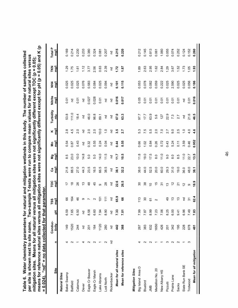
46

Tabl

e 6.

Wat

er c

hem

istr

y pa

ram

eter

s fo

r nat

ural

and

miti

gatio

n w

etla

nds

in th

is s

tudy

. Th

e nu

mbe

r of s

ampl

es c

olle

cted

per s

ite is

sho

wn

next

to s

ite n

ame.

Tw

o-sa

mpl

e T-

test

s w

ere

run

to c

ompa

re m

ean

valu

es fo

r the

nat

ural

site

s ve

rsus

miti

gatio

n si

tes.

Mea

ns fo

r all

natu

ral v

ersu

s al

l miti

gatio

n si

tes

wer

e no

t sig

nific

antly

diff

eren

t exc

ept T

OC

(p =

0.0

5);

mea

ns fo

r ref

eren

ce n

atur

al s

ites

vers

us a

ll m

itiga

tion

site

s w

ere

not s

igni

fican

tly d

iffer

ent e

xcep

t for

pH

(p =

0.0

5) a

nd K

(p=

0.02

4).

“nd”

= n

o da

ta c

olle

cted

for t

hat p

aram

eter

.

Site

nC

ondu

c-tiv

itypH

TSS

mg/

lTO

Cm

g/l

Ca

mg/

lM

gm

g/l

Mn

mg/

lK mg/

lTu

rbid

itynt

uN

itrite

mg/

lN

H4

mg/

lTK

Nm

g/l

Tota

l Pm

g/l

Nat

ural

Site

s

Bake

r Sw

amp

414

96.

5966

1721

.88.

50.

542.

853

.80.

010.

025

1.29

0.16

9Ba

llfie

ld2

1520

7.65

164

1888

.523

.00.

87

4.5

111.

0nd

0.02

51.

75

0.21

4

Cal

amus

124

46.

5046

2627

.010

.00.

432.

018

.40.

010.

025

1.61

0.23

0

Dev

er4

ndnd

913

44.3

14.8

ndnd

ndnd

0.07

61.

120.

233

Eagl

e C

r Bea

ver

220

18.

587

4823

.55.

00.

32

2.0

46.0

0.02

70.

583

3.77

0.38

0

Eagl

e C

r Mar

sh

216

46.

602

4516

.55.

00.

552.

096

.80.

028

0.08

42.

56

0.32

4

Lake

Abr

ams

111

207.

9410

19

66

.514

.00.

2410

.0

89.1

0.01

0.02

50.

630.

081

Lodi

Nor

th2

280

8.90

111

2838

.511

.50.

041.

0nd

nd0.

094

2.39

0.20

7

Ric

kenb

acke

rnd

ndnd

ndnd

ndnd

ndnd

ndnd

ndnd

nd

Mea

n fo

r all

natu

ral s

ites

442

7.33

65.9

22.6

38.1

11.7

0.44

3.

567

.00.

016

0.10

11.

72

0.21

5

Mea

n fo

r ref

eren

ce s

ites

368

7.01

6626

.532

.210

.50.

552.

763

.30.

017

0.11

51.

870.

220

Miti

gatio

n Si

tes

Big

Isla

nd A

rea

D4

267

7.99

113

30

38.0

11.8

0.66

5.

397

.70.

050.

053

1.89

0.

212

Blue

bird

238

37.

8730

3844

.019

.01.

02

7.5

17.7

0.01

0.07

82.

630.

145

JMB

263

28.

9961

10

52

.517

.50.

845.

563

.90.

010.

082

2.95

0.81

3

Med

allio

n N

o. 2

01

1650

7.23

2

1520

.08.

00.

26

2.0

5.6

0.01

0.05

91.

620.

061

New

Alb

any

HS

142

67.

0631

60.0

11.0

0.72

7.0

127

0.01

0.22

22.

841.

060

Pizz

utti

320

18.

2549

13

29.3

9.0

0.43

2.

722

.90.

010.

025

1.29

0.

055

Prai

rie L

ane

234

26.

0013

1231

.08.

05.

249.

07.

30.

012.

590

3.67

0.07

4

Sack

s2

195

9.41

1321

19.0

8.5

0.11

2.5

2.7

0.01

0.02

51.

520.

252

Slat

e R

un B

ank

SE1

228

6.96

nd12

36

.0

11.0

3.59

1.0

ndnd

0.02

51.

730.

124

Trot

woo

d3

678

7.49

319

48

.022

.70.

46

4.0

21.6

0.01

0.05

61.

05

0.15

2M

ean

for a

ll m

itiga

tion

481

7.83

62.4

18.9

38.1

13.5

0.95

24.

646

.50.

016

0.18

61.

930.

260

Table 7. Comparison of median (25th - 75th percentile) water chemistry of wetlands (n ~ 200 water samples depending on parameter) from Ohio EPAreference wetland data set, 1996-2003. Impoundments included in riverine mainstem or riverine headwater. Notable values underlined. Note chemicalsimilarities of slope systems, coastal marshes, and Lake Plains sand prairies. Note differences in bog systems from other types.

Description HGM class pH TSS mg/l TOC(%) Ca mg/l Fe mg/l Mg mg/l Cl - mg/l NH4 mg/l P total mg/l

Bogs weaklyombrotrophic

--- 41.8(---) 59.0(---) 15.5(---) 17.1(---) 4.5(---) 4.3(---) 0.13(---) 0.59(---)

Bogs moderate tostronglyombrotrophic

--- 18.0(3-45) 45.0(16-71) 3.0(2-7) 1.4(0.5-3.7) 1.0(0.5-2.0) <2.5 0.025(0.025-0.09 0.07(0.025-0.18)

Depressionalmarshes

depression 6.5(5.3-6.9) 9.5(7-42) 14.0(11-22) 35.0(24-45) 1.2(1.0-2.0) 12.0(7-14) 9.8(3-125) 0.025(0.025-0.12) 0.17(0.09-0.29)

Mainstemmarshes

riverinemainstem

7.7(7.0-7.8) 47.0(20-177) 11.5(8-17) 43.0(36-73) 2.2(1.5-9.6) 11.0(9-21) 17.0(12-176) 0.055(0.025-0.241) 0.12(0.07-0.24)

Headwatermarshes

riverineheadwater

6.9(6.6-7.3) 27.0(17-68) 18.0(8-41) 24.0(17-51) 3.6(1.5-7.4) 6.0(5-17) 9.0(3-24) 0.025(0.025-0.054) 0.19(0.09-0.51)

Mitigationmarshes

mostlyimpoundments

7.6(7.1-8.7) 33.0(12-96) 15.5(12-20) 31.0(20-43) 2.1(1.3-5.4) 10.0(7-14) 10.0(3-17) 0.025(0.025-0.088) 0.14(0.07-0.27)

Coastalmarshes

Lake ErieCoastal

8.2(7.8-8.3) 77.0(13-98) 9.5(6-14) 58.0(39-65) 3.2(0.3-4.2) 15.0(12-21) 26.9(17-93) 0.051(0.025-0.074) 0.16(0.05-0.17)

Calcareousfens

slope 7.9(---) 2.5(2.5-2.5) 7.4(3-12) 59.0(46-91) 0.94(0.95-2.0) 30.0(28-38) 19.8(17-45) <0.025 0.25(0.03-0.51)

Fen meadows slope --- 18.8(---) 13.6(---) 48.0(---) 3.9(---) 11.5(---) 32.8(---) 0.042(---) 0.12(---)

Forest seeps slope --- --- --- --- --- --- --- --- ---

Wet meadows all except slope --- --- --- --- --- --- --- --- ---

Lake PlainsSand Prairies

mostlydepressions

7.1(7.0-7.3) 7.0(6-152) 35.0(35-44) 19.0(19-57) 2.2(0.6-2.6) 6.0(5-10) <2.5 0.025(0.025-0.13) 0.08(0.07-0.15)

Forest vernalpools

depression 7.0(5.4-7.4) 14.5(3-49) 16.5(6-23) 36.5(18-66) 0.80(0.5-1.5) 11.0(3-14) <2.5 0.08(0.025-0.17) 0.14(0.09-0.28)

Shrub vernalpools

depression 6.8(6.5-7.2) 11.0(5-24) 29.0(15-35) 29.0(16-43) 0.95(0.7-1.9) 8.0(5-14) 2.5(2.5-6) 0.085(0.025-0.20) 0.25(0.10-0.52)

Wet woods depression 7.4(---) 11.0(8-125) 39.0(33-41) 22.0(5-51) 2.3(1.6-3.1) 5.0(2-8) 2.5(2.5-19) 0.05(0.025-0.286) 0.12(0.09-0.42)

Mainstemswamp forests

riverinemainstem

7.0(6.2-7.2) 25.0(14-59) 18.0(16-23) 42.5(15-61) 1.9(1.4-4.4) 11.0(4-16) 2.5(2.5-42) 0.19(0.07-1.27) 0.48(0.22-0.76)

Mainstemshrub swamps

riverinemainstem

6.8(6.1-6.8) 38.0(27-73) 14.0(10-14) 3.1(2.1-8.8) 5.0(4-8) 2.5(2.5-7.6) 0.025(0.025-0.132) 0.12(0.08-0.23)

Table 8a. Standard agronomic soil chemistry parameters for natural and mitigation wetlands (n = 5). %OM determined by Walkly-Black Method, %OCdetermined by CHN Analyzer (See methods section). * = low %OM values due to underestimation of %OM by Walkly-Black method in high carbon soils.

site %OM %OC %Nweak P

ppmstrong P

ppm K ppm Mg ppm Ca ppm Na ppm pH CEC

Natural sites

Baker Swamp 4.1 + 0.36 5.36 + 1.0 0.49 + 0.07 17.2 + 3.2 71.4 + 6.6 225 + 91 264 + 21 1267 + 251 0 5.20 + 0.37 15.2 + 1.6

Ballfield 7.3 + 0.86 12.0 + 2.0 0.87 + 0.15 8.6 + 1.4 19.0 + 3.7 61 + 14 377 + 69 2229 + 267 61.2 + 37.5 6.40 + 0.24 15.9 + 1.3

Calamus 8.6 + 0.61* 27.7 + 4.2 2.36 + 0.50 12.0 + 4.2 24.0 + 9.1 79 + 24 568 + 144 2164 + 268 0 6.04 + 0.25 18.2 + 2.1

Dever 6.8 + 0.44 9.8 + 1.9 0.80 + 0.14 15.4 + 2.5 44.2 + 6.4 108 + 7 547 + 60 2249 + 147 0 5.66 + 0.32 21.3 + 0.5

Eagle Cr Beaver 8.5 + 0.70* 28.2 + 5.5 2.12 + 0.44 12.8 + 2.9 30.4 + 10.8 44 + 9 263 + 39 2022 + 252 0 5.06 + 0.10 20.2 + 1.9

Eagle Cr Marsh 5.6 + 0.19 6.7 + 0.6 0.54 + 0.04 10.6 + 2.5 37.0 + 6.8 70 + 9 145 + 12 1039 + 115 0 4.86 + 0.05 12.0 + 1.1

Lake Abrams 6.2 + 0.34 11.4 + 2.5 0.78 + 0.22 11.4 + 2.9 86.6 + 22.3 60 + 11 277 + 27 2147 + 192 417.4 + 82.1 5.88 + 0.30 18.7 + 1.4

Lodi North 10.9 + 0.21* 27.4 + 3.1 1.66 + 0.14 10.4 + 1.4 33.0 + 4.4 38 + 10 371 + 26 3052 + 360 0 5.72 + 0.19 23.7 + 2.1

Rickenbacker 5.3 + 0.44 7.4 + 1.7 0.53 + 0.09 9.2 + 1.2 43.8 + 5.3 164 + 18 338 + 38 1734 + 96 0 5.38 + 0.10 16.9 + 1.2

Mitigation sites

Big Island Area D 3.0 + 0.29 2.5 + 0.3 0.28 + 0.02 4.0 + 0.6 18.8 + 3.1 171 + 23 372 + 31 1653 + 118 0 5.90 + 0.18 14.3 + 0.8

Bluebird 2.2 + 0.36 2.2 + 0.4 0.23 + 0.04 3.0 + 0.5 15.8 + 2.0 106 + 6 317 + 19 1144 + 33 0 5.96 + 0.17 10.4 + 0.2

JMB 2.0 + 0.27 2.5 + 0.3 0.26 + 0.02 9.0 + 0.9 41.2 + 6.2 101 + 7 345 + 28 2046 + 115 30.0 + 30.0 7.10 + 0.10 13.5 + 0.8

Medallion No. 20 1.7 + 0.17 1.9 + 0.2 0.22 + 0.02 1.6 + 0.4 12.6 + 0.8 108 + 2 295 + 36 1208 + 52 0 5.66 + 0.18 11.5 + 0.8

New Albany HS 5.8 + 0.72 4.3 + 0.9 0.32 + 0.02 24.0 + 3.6 62.0 + 8.1 134 + 9 325 + 36 2353 + 266 0 7.38 + 0.10 14.8 + 1.4

Pizzutti 1.6 + 0.21 1.3 + 0.2 0.17 + 0.02 2.0 + 0.4 7.4 + 0.8 64 + 2 199 + 33 984 + 91 0 6.12 + 0.07 7.8 + 0.8

Prairie Lane 2.7 + 0.19 2.4 + 0.2 0.24 + 0.02 5.8 + 0.2 21.6 + 4.2 92 + 14 212 + 12 1395 + 65 0 5.78 + 0.12 11.2 + 0.3

Sacks 3.4 + 0.24 3.6 + 0.5 0.32 + 0.04 14.8 + 3.8 75.2 + 6.8 137 + 14 337 + 26 1617 + 123 0 5.66 + 0.05 14.4 + 0.9

Slate Run Bank SE 2.3 + 0.09 2.1 + 0.3 0.20 + 0.01 2.2 + 0.4 15.0 + 1.6 101 + 14 266 + 23 1398 + 162 0 6.18 + 0.28 10.9 + 0.7

Trotwood nd nd nd nd nd nd nd nd nd nd nd

Table 8b. Additional soil chemistry parameters for natural and mitigation wetlands (n = 1) and exchangeable ions (%K, %Ca, %Mg, %H)(n = 5). Data on TOC determined by U.S. EPA 415.1.

site TOC (%) %solidsAmmonia

mg/kgexchangeable

K (%)exchangeable

Ca (%)exchangeable

Mg (%)particle size>50um (%)

particle size2-50 um (%)

particle size<2 um (%)

Natural sites

Baker Swamp 5 58.6 110 4.1 + 1.9 43.0 + 9.1 15.0 + 2.0 23.7 43 11.2

Ballfield 9 48 22 0.9 + 0.2 69.3 + 4.0 19.4 + 2.4 59.2 37 1.8

Calamus 39 15.4 120 1.0 + 0.3 59.2 + 0.8 24.6 + 3.3 61.3 22.1 0

Dever 12 40 27 1.3 + 0.1 53.0 + 3.9 21.5 + 2.6 58 27 3.6

Eagle Cr Beaver 42 16.2 110 0.6 + 0.1 49.9 + 3.0 10.7 + 0.6 83.6 8.2 0

Eagle Cr Marsh 3 69.7 93 1.5 + 0.1 43.0 + 1.7 10.2 + 0.3 52.3 37.5 2.8

Lake Abrams 13 46.6 16 0.8 + 0.2 57.9 + 5.3 12.5 + 1.3 33.1 46.4 5.8

Lodi North 20 37.9 57 0.4 + 0.1 64.5 + 4.6 13.2 + 0.3 60.7 28.9 4.2

Rickenbacker 11 50.1 7 2.5 + 0.2 51.8 + 2.1 16.5 + 1.1 52.5 33.2 4.2

Mitigation sites

Big Island Area D 2 73.8 20 3.0 + 0.3 57.6 + 2.6 21.5 + 1.0 29.8 43.7 9.5

Bluebird 1 79.5 35 2.6 + 0.2 55.2 + 2.0 25.5 + 1.7 52.7 30.4 5.7

JMB 2 71.8 5 1.9 + 0.1 75.9 + 1.4 21.3 + 1.0 31.3 48.8 6.6

Medallion No. 20 1 70.6 15 2.5 + 0.2 53.2 + 3.0 21.3 + 2.1 33.5 41.2 4

New Albany HS 2 66.7 32 2.4 + 0.3 79.1 + 1.9 18.5 + 1.7 41 44.8 4.1

Pizzutti 1 74.3 24 2.2 + 0.2 63.6 + 1.7 20.9 + 1.1 48.9 40.2 5.5

Prairie Lane 2 69.2 21 2.1 + 0.3 62.1 + 2.0 15.7 + 0.6 31.2 47 10.2

Sacks 2 70.8 30 2.5 + 0.3 56.1 + 1.1 19.4 + 0.3 37.6 46.4 5.4

Slate Run Bank SE 1 82.2 5 2.4 + 0.3 63.7 + 3.5 20.3 + 0.9 32.6 48.8 5.7

Trotwood 2 76 19 nd nd nd 58.5 27.7 1.3

50

Table 9. Summary of mean soil parameters of natural and mitigation wetlands. Valuesare average of 9 natural sites and 10 mitigation sites listed in Table 8a and 8b. p-values are results of two sample t-test. SE = standard error of the mean. ns =nonsignificant, i.e. p > 0.1

parameter unitsmean (SE)

natural sitesmean (SE)

mitigation sites p

pH na 5.58 + 0.10 6.19 + 0.10 < 0.0001

Organic Matter (Walkly-Black) % 7.03 + 0.33 2.76 + 0.21 < 0.0001

Organic Carbon (CHN analyzer) % 15.1 + 1.6 2.45 + 0.16 < 0.0001

TOC (EPA Method 415.1) % 17.1 + 4.7 1.60 + 0.16 0.011

%solids % 42.5 + 6.0 73.5 + 1.5 0.0007

Nitrogen, total % 1.12 + 0.13 0.24 + 0.01 < 0.0001

Ammonia ug/g 62.4 + 15.0 20.6 + 3.3 0.028

P, weak (Bray 1) ug/g 11.96 + 0.89 7.38 + 1.20 0.003

P, strong (Bray 2) ug/g 43.4 + 4.3 30.0 + 3.7 0.021

P, total ug/g 1156 + 252 669 + 91 0.099

K ug/g 94.5 + 13.0 112.5 + 5.7 ns

Mg ug/g 296.4 + 12.0 350.0 + 27.0 0.074

Ca ug/g 1989 + 109 1533 + 74 0.0009

Na ug/g 53 + 22 3.3 + 3.3 0.027

CEC na 18.0 + 0.7 12.1 + 0.4 < 0.0001

exchangeable K % 1.47 + 0.25 2.40 + 0.09 0.0011

exchangeable Mg % 15.97 + 0.90 20.50 + 0.54 0.0001

exchangeable Ca % 54.6 + 1.9 62.9 + 1.5 0.0007

particle size >50µm % 53.8 + 3.2 39.7 + 5.7 0.054

particle size 2µm - 50µm % 31.5 + 3.9 41.9 + 2.3 0.038

particle size <2µm % 3.7 + 1.1 5.8 + 0.8 ns

51

Tabl

e 10

. C

ompa

rison

of m

edia

n (2

5th -

75th

per

cent

ile) s

oil c

hem

istr

y of

wet

land

s (n

~ 2

50 s

oil s

ampl

es d

epen

ding

on

para

met

er) f

rom

Ohi

o EP

A re

fere

nce

wet

land

dat

a se

t, 19

96-2

003.

Im

poun

dmen

ts in

clud

ed in

rive

rine

mai

nste

m o

r riv

erin

e he

adw

ater

dep

endi

ng o

n th

eir l

ands

cape

pos

ition

. N

otab

le v

alue

sun

derli

ned.

Not

e si

mila

ritie

s in

soi

l che

mis

try

of s

lope

sys

tem

s, c

oast

al m

arsh

es, a

nd L

ake

Plai

ns s

and

prai

ries.

Des

crip

tion

HG

M c

lass

%so

lids

TOC

%Al

g/k

gC

a g/

kgFe

g/k

gM

g g/

kgK

g/k

gN

H4

mg/

kgP

tota

l g

/kg

Bogs

bog

18.9

(15-

27)

41.7

(25-

43)

5.9(

3-51

)4.

7(4-

12)

5.2(

4-11

)2.

1(0.

8-4.

1)2.

6(2-

5)18

.5(8

-128

)10

70(3

83-1

840)

Dep

ress

iona

l mar

shes

depr

essi

on62

.4(4

7-68

)3.

6(3-

7)27

.2(1

2-36

)3.

7(5-

13)

17.1

(11-

21)

5.1(

4-6)

5.4(

2-6)

39.0

(22-

60)

1270

(784

-192

5)

Mai

nste

m m

arsh

esriv

erin

e m

ains

tem

46.6

(40-

59)

3.9(

2-8)

37.2

(23-

51)

3.2(

2-9)

28.4

(16-

36)

3.3(

3-6)

6.1(

4-10

)54

.0(2

6-91

)79

0(64

0-11

35)

Hea

dwat

er m

arsh

esriv

erin

e he

adw

ater

46.6

(41-

59)

4.1(

2-15

)30

.7(1

8-60

)3.

1(1-

6)17

.9(1

3-31

)2.

5(2-

6)4.

9(3-

11)

77.5

(22-

118)

673(

436-

1142

)

Miti

gatio

n m

arsh

esm

ostly

impo

undm

ents

73.3

(70-

76)

2.0(

1-2)

33.8

(26-

41)

3.0(

2-5)

25.7

(20-

31)

4.2(

3-5)

7.2(

5-9)

24.0

(8-4

0)59

2(47

5-80

2)

Coa

stal

mar

shes

Lake

Erie

Coa

stal

54.9

(42-

62)

4.1(

3-6)

32.6

(25-

43)

12.8

(7-3

2)21

.6(1

9-29

)5.

9(5-

9)8.

6(5-

11)

30.0

(23-

65)

826(

556-

1315

)

Cal

care

ous

fens

slop

e30

.0(2

4-41

)24

.5(7

-27)

3.9(

0.6-

6.9)

45.6

(31-

140)

7.5(

1-24

)5.

1(2-

7)14

.6(1

0-25

)52

.0(4

4-21

0)61

8(34

6-13

40)

Fen

mea

dow

ssl

ope

48.0

(13-

57)

9.0(

6-34

)13

.5(6

-31)

3.9(

3-29

)13

.9(1

0-19

)2.

7(2-

4)2.

9(2.

6-3.

2)22

.0(1

6-98

)97

1(95

7-12

60)

Fore

st s

eeps

slop

e38

.0(3

1-43

)9.

3(6-

20)

40.0

(13-

49)

6.6(

3-14

)27

.2(1

3-44

)3.

4(2-

5)5.

0(2-

9)21

.3(8

-63)

784(

568-

1054

)

Wet

mea

dow

sal

l exc

ept s

lope

55.9

.0(--

-)3.

1(---

)43

.9(--

-)4.

3(---

)37

.6(--

-)4.

3(---

)7.

0(---

)26

.0(--

-)90

8(---

)

Lake

Pla

ins

Sand

Pra

iries

mos

tly d

epre

ssio

ns61

.0(3

9-71

)9.

5(5-

14)

11.4

(8-1

9)7.

8(4-

28)

9.5(

7-14

)1.

6(1-

3)0.

76(0

.51-

1.6)

34.0

(21-

63)

337(

202-

555)

Fore

st v

erna

l poo

lsde

pres

sion

58.1

(38-

68)

5.4(

2.9-

11.1

)30

.0(9

-41)

6.5(

4-13

)12

.8(8

-34)

3.7(

3-6)

5.1(

1-7)

49.0

(27-

95)

1060

(593

-218

0)

Shru

b ve

rnal

poo

lsde

pres

sion

41.9

(32-

54)

10.1

(6-1

6)37

.3(1

1-51

)7.

1(4-

10)

13.6

(6-1

9)3.

7(2-

6)3.

5(1-

6)57

.2(2

9-10

1)14

90(7

41-1

955)

Wet

woo

dsde

pres

sion

57.4

(48-

71)

6.6(

4-9)

27.2

(9-4

64.

8(4-

12)

15.0

(6-2

0)2.

6(1-

6)3.

2(1-

12)

39.5

(7-3

9)84

1(40

1-12

15)

Mai

nste

m s

wam

p fo

rest

sriv

erin

e m

ains

tem

66.1

(59-

70)

2.9(

2-4)

36.5

(20-

49)

3.2(

0.8-

7.5)

24.8

(3-3

0)3.

3(3-

5)6.

5(4-

10)

36.0

(21-

67)

626(

511-

988)

Mai

nste

m s

hrub

sw

amps

river

ine

mai

nste

m62

.1(5

2-70

)3.

7(3-

5)36

.0(1

8-46

)3.

0(0.

6-6.

7)20

.8(8

-28)

4.2(

3-9)

5.8(

3-8)

56.6

(21-

79)

904(

632-

1460

)

52

Table 11. Vegetation community attributes of natural and mitigationwetlands including species richness, Vegetation Index of BioticIntegrity scores (VIBI), Floristic Quality Assessment Index scores(FQAI), and biomass production (mean of 8 samples per site).Wetland Type Species VIBI FQAI Biomass

Natural sites

Baker N 31 71 24.7 23.7

Ballfield N 61 73 31 na

Beaver Pond N 25 82 25.0 31.9

Calamus N 24 57 21.5 39.4

Dever N 26 9 15.8 44.2

Eagle Creek N 42 81 22.9 52.4

Lake Abrams N 20 33 17 41.4

Lodi N 19 45 15.8 33.1

Rickenbacker N 31 67 17.7 11.7

Mitigation Sites

Big Island C 34 50 14.7 30.6

Bluebird C 33 20 14.4 16.4

JMB C 29 16 14.5 7.1

Medallion C 39 46 18.1 5.2

New Albany C 23 16 12.0 58.6

Pizzutti C 17 30 14.7 21.2

Prairie Lane C 28 43 15.0 26.5

Sacks C 13 19 9.8 20.9

Slate Run C 27 16 15.4 naTrotwood C 13 16 13.6 1.9

Table 12. Summary of mean vegetation attributes of naturaland mitigation wetlands. Values recoded are an average ofthe 9 natural sites and 10 mitigation sites cited above (Table6a). Error recorded is the standard error. (*Ballfield and SlateRun omitted as a statistical outliers).

Vegetation attributes Natural Mitigation P-value

Species richness 31.0 ± 4.4 25.6± 2.8 0.22

VIBI score 57.6 ± 8.1 27.2 ± 4.6 0.005

FQAI score 21.6 ± 1.7 14.2± 0.7 0.004

Biomass Production (g/0.1m2) 34.7 ± 3.5 20.9 ± 5.7* 0.04

53

Table 13. Mean amount of ON-SITE litter lost for each wetland at all collection periods. Valuesrecorded are an average of 5 stations (n = 6 natural and n =9 created wetlands). K values arecalculated based on the average mass lost for each wetland.

Wetland Mass lost (g) 1st

(g lost.day-1)Mass lost (g) 2nd

(g lost.day-1)Mass lost (g) 3rd

(g lost.day-1)k-value 1st k-value 2nd k-value 3rd

Natural sites

Baker Swamp 5.42 (0.143) 6.06 (0.068) 6.13 (0.017) 0.0205 0.0103 0.00276

Ballfield 4.24 (0.118) 6.64 (0.076) 5.96 (0.019) 0.0153 0.0125 0.00295

Calamus 4.92 (0.129) 6.00 (0.067) 6.56 (0.019) 0.0178 0.0103 0.00315

Dever 3.46 (0.105) 5.12 (0.06) 6.40 (0.022) 0.0129 0.0084 0.00345

Lodi 6.30 (0.154) 7.10 (0.082) 6.83 (0.019) 0.0243 0.0142 0.00382

Rickenbacker 2.84 (0.079) 4.24 (0.048) 5.68 (0.019) 0.0093 0.0062 0.00281

Mitigation sites

Big Island Area D 2.94 (0.072) 2.04 (0.023) 3.38 (0.011) 0.0085 0.0026 0.00137

Bluebird 5.36 (0.141) 5.76 (0.065) na 0.0202 0.0096 na

JMB 3.18 (0.088) 4.38 (0.053) 5.62 (0.019) 0.0106 0.0069 0.00280

Medallion No. 20 4.82 (0.134) 5.00 (0.061) 6.38 (0.021) 0.0183 0.0085 0.00341

New Albany HS 4.90 (0.129) 6.22 (0.070) 6.30 (0.021) 0.0177 0.0109 0.00328

Pizzutti 5.12 (0.155) 4.92 (0.058) 5.10 (0.017) 0.0217 0.0080 0.00243

Prairie Lane 2.68 (0.065) 2.40 (0.028) 3.67 (0.012) 0.0076 0.0032 0.00152

Sacks 2.60 (0.072) 4.80 (0.055) na 0.0084 0.0075 naSlate Run Bank SE 3.72 (0.098) 4.90 (0.050) 5.34 (0.018) 0.0122 0.0076 0.00254

Table 14. Summary of both the mean amount of on-site litter lost and the k-value of natural and mitigation wetlands. Values recorded are an average ofthe 6 natural sites and 9 created sites cited above (mean ± standard error).

Natural Created P-value

Mass lost (g) 1st 4.53± 0.52 3.92± 0.37 0.07

Mass lost (g) 2nd 5.86± 0.42 4.49± 0.47 0.05

Mass lost (g) 3rd 6.26± 0.17 5.11± 0.48 0.05

Mass lost, g.day-1 1st 0.121+ 0.01 0.106+0.01 0.35

Mass lost, g.day-1 2nd 0.067+0.005 0.051+0.005 0.06

Mass lost, g.day-1 3rd 0.019+0.001 0.017+0.001 0.23

k-value 1st 0.0167±0.002 0.0139± 0.001 0.32

k-value 2nd 0.0094± 0.0001 0.0078± 0.001 0.36k-value 3rd 0.0030± 0.001 0.0025±0.001 0.08

54

Table 15. Mean amount of CONTROL litter lost for each wetland at all collection periods. Values recorded are an average of 3 stations. Values recorded are an average of 3stations except for values marked with * where n = 1 (n = 9 natural and n = 9 mitigationwetlands; 6 natural sites sampled in 2001 and 3 in 2002). K values are calculated basedon the average mass lost for each wetland.

WetlandMean masslost (g) 1st

Mean masslost (g) 2nd

Mean masslost (g) 3rd k-value 1st k-value 2nd k-value 3rd

Natural

Baker Swamp 6.07 (0.105) 6.63 (0.061) 7.10 (0.020) 0.0161 0.0101 0.0034

Ballfield 4.73 (0.086) 6.80 (0.064) 7.3 (0.022) 0.0116 0.0107 0.0039

Calamus 7.10 (0.122) 8.00 (0.073) 8.13 (0.023) 0.0213 0.0148 0.00467

Dever 5.30 (0.010) 5.90 (0.056) 7.1 (0.022) 0.0142 0.0085 0.00392

Lodi North 7.13 (0.119) 7.70 (0.072) 7.20 (0.018) 0.0208 0.0137 0.00397

Eagle Cr Beaver 4.80 0.044)* 6.20 0.023) 6.43 0.022) 0.0061 0.0036 0.0035

Eagle Cr Marsh 5.35(0.050) 6.38(0.024) 5.95(0.021) 0.0071 0.0038 0.0031

Lake Abrams 4.70(0.044) 4.20(0.016)* 4.80(0.017)* 0.0059 0.0020 0.0023

Rickenbacker 4.17 (0.072) 5.83 (0.053) 6.00 (0.019) 0.0093 0.0079 0.00285

Mitigation

Big Island Area D 5.73 (0.094) 7.07 (0.066) 5.90 (0.018) 0.0142 0.0115 0.00278

Prairie Lane 4.20 (0.070) 3.43 (0.032) 3.90 (0.012) 0.0091 0.0040 0.00154

Sacks 3.53 (0.064) 6.57 (0.062) 5.05 (0.015) 0.0079 0.0101 0.00208

JMB 3.97 (0.063) 4.93 (0.044) 5.80 (0.018) 0.0090 0.0061 0.00269

Slate Run Bank SE 4.47 (0.077) 4.07 (0.037) 4.37 (0.014) 0.0102 0.0048 0.00179

Pizzutti 5.47 (0.103) 6.37 (0.061) 6.00 (0.019) 0.0149 0.0097 0.00292

New Albany HS 5.85 (0.113) 6.20 (0.060) 5.45 (0.017) 0.0160 0.0094 0.00248

Bluebird 6.60 (0.127) 6.93 (0.064) na 0.0196 0.0115 naMedallion No. 20 6.00 (0.107) 6.05 (0.059) 6.25 (0.020) 0.0164 0.0091 0.00308

Table 16. Summary of both the mean amount of control litter lost andthe k-values for natural and Mitigation wetlands. Values recoded arean average of the 6 natural sites and 9 created sites cited above (mean± standard error).

Natural Created P-value

Mass lost (g) 1st 5.75± 0.32 5.14± 0.26 0.15

Mass lost (g) 2nd 6.81± 0.22 5.93± 0.29 0.02

Mass lost (g) 3rd 7.14 ± 0.28 5.34 ± 0.29 0.001

Mass lost g.day-1 1st 0.100+.008 0.091+0.008 0.39

Mass lost g.day-1 2st 0.063+0.003 0.098+0.043 0.44

Mass lost g.day-1 3st 0.021+0.001 0.017+0.001 0.008

k–value 1st 0.0156± 0.002 0.0130± 0.001 0.32

k-value 2nd 0.0102± 0.001 0.0090± 0.001 0.44k–value 3rd 0.004 ± 0.0003 0.002 ± 0.0001 0.001

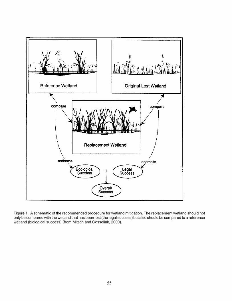
55

Figure 1. A schematic of the recommended procedure for wetland mitigation. The replacement wetland should notonly be compared with the wetland that has been lost (the legal success) but also should be compared to a referencewetland (biological success) (from Mitsch and Gosselink, 2000).

56

Decomposition

Nutrient leaching rate

Aboveground biomass

Soil composition

Detritus

Plant community composition

Water Chemistry

Nutrient uptake

Organic matterproduction

VIBI

Biogeochemical indicators

Soil

Figure 2. Conceptual model of the ecosystem components included in this study including structural components,processes, and indicators that are empirically derived to indicate ecosystem condition.

57

x4 x5 Samples 4 and 5: taken half way between the center and the far edge, \ / at a 45 degree angle from initial line (i.e., line made by samples 1 - 3). \ /

x3 Sample 3: taken and the approximate center of the wetland |x2 Sample 2: taken half way between 1 and the approximate center of the wetland |x1 Sample 1: taken approximately 10 m from wetland boundary, near well

Figure 3. Sampling scheme used to collect soil samples at all wetlands.

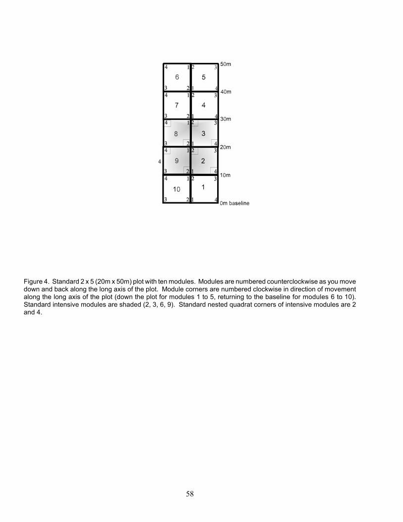
58

Figure 4. Standard 2 x 5 (20m x 50m) plot with ten modules. Modules are numbered counterclockwise as you movedown and back along the long axis of the plot. Module corners are numbered clockwise in direction of movementalong the long axis of the plot (down the plot for modules 1 to 5, returning to the baseline for modules 6 to 10).Standard intensive modules are shaded (2, 3, 6, 9). Standard nested quadrat corners of intensive modules are 2and 4.

59

-120

-100

-80

-60

-40

-20

0

M N

Figure 5a. Box plots for four hydrological parameters for mitigation versus natural wetlands in the 2001 fieldseason. Parameters are a) percent time groundwater was in the root zone (top 30 cm of soil profile); b)mean depth to groundwater (cm); c) mean maximum depth (cm); and d) mean minimum depth togroundwater (cm). Positive values in b – d indicate groundwater levels were above the soil surface. Meanswere evaluated using unpaired t-tests (p values shown to indicate means that are significantly different).

p = 0.04

nsd

p = 0.04

p=0.08

a) b)

d)c)

60

-20

0

20

40

60

80

100

M N-100

-90-80-70-60-50-40-30-20-10

0

M N

-110

-100

-90

-80

-70

-60

-50

-40

-30

M N

Figure 5b. Box plots for four hydrological parameters for mitigation versus natural wetlands in the 2002 fieldseason. Parameters are a) percent time groundwater was in the root zone (top 30 cm of soil profile); b)mean depth to groundwater (cm); c) mean maximum depth (cm); and d) mean minimum depth togroundwater (cm). Positive values in b – d indicate groundwater levels were above the soil surface. Meanswere evaluated using unpaired t-tests (p values shown to indicate means that are significantly different).nsd = nonsignificant difference.

p = 0.06 p = 0.087

nsd nsd

a) b)

d) c)

61

������������������������������������������������������������������������������������������������������������������������������������������������������������������������������������������������������

������������������������������������������������������������������������������������������������������������������������������������������������������������������������������������������������������������������������������������������������������������������������������������������������

������������������������������������������������������������������������������������������������������������������������������������������������������������������������������������������������������������������������������������������������������������������������������������������������������������������������������������

���������������������������������������������������������������������������������������������������������������������������������������������������������������������������������������������������������������������������������������������������������������

������������������������������������������������������������������������������������������������������������������������������������������������������������������������������������

������������������������������������������������������������������������������������������������������������������������������������������������������������������������������������������������������

0

10

20

30

40

50

60

70

surface water groundwater % time in root zone

Wat

er le

vel (

cm) o

r %�������� Natural sites�������� Mitigation sites

Figure 6. Mean surface water levels, depth to groundwater and the percent time water was found in the rootzone for natural and mitigation wetlands in the 2001 growing season (mean + standard deviation). Meansurface water levels were shallower at natural wetlands, mean depth to groundwater was shallower atnatural wetlands, and percent time water was in the root zone was longer at natural wetlands.

62

16-Aug 24-Nov 4-Mar 12-Jun 20-Sep

-100

-50

0

dept

h (c

m)

Big Island Area D

Index = 1.5.spring 2002. FlashinessWell failure fall 2001 towith summer drawdown.Strong season signatureprecipitation and sheet flow.Impoundment. Hydrology:Mitigation Wetland.

16-Aug 24-Nov 4-Mar 12-Jun 20-Sep

-100

-50

0

dept

h (c

m)

Ballfield

Flashiness Index = 1.9.collected in 2000 shows "flat" hydrograph year round.water, precipitation. Well failure after fall 2001. Datainto slope wetland. Hydrology: flood events, groundNatural Wetland. Riverine Depression grading upslope

17-Aug 25-Nov 5-Mar 13-Jun 21-Sep

-100

-50

0

dept

h (c

m)

Baker Swamp

fall 2001 to spring 2002. Flashiness Index = 2.8.headwater streams. Seasonal signature. Well failurebeaver activity. Hydrology = precipitation, sheet flow,Natural Wetland. Headwater Depression with some

Figure 7. Hydrographs for Baker Swamp (natural), Ballfield (natural), and Big Island Area D (mitigation) sitesfrom June 1, 2001 to October 1, 2002. Gap in hydrograph for Baker Swamp due to vandalization of well.Gaps in hydrographs at Ballfield and Big Island Area D due to failure of well caused by a manufacturingdefect.

63

20-Sep12-Jun4-Mar24-Nov16-Aug

0

-50

-100

dept

h (c

m)

Bluebird Mitigation Wetland. Depression. Hydrology =precipitation, sheet flow. Site inundated formuch of year. Disconnect between surfaceand ground water. Flashiness index = 2.0.

16-Aug 24-Nov 4-Mar 12-Jun 20-Sep

-100

-50

0

dept

h (c

m)

Dever

Index = 1.5.spring 2002. FlashinessWell failure fall 2001 toStrong seasonal signature.and possible tile discharges.Hydrology = precipitation,located in ag field.Natural Wetland. Depression

16-Aug 24-Nov 4-Mar 12-Jun 20-Sep

-100

-50

0

dept

h (c

m)

Calamus

superimposed. Flashiness Index = 1.6.stormwater inputs. Seasonal signature with rain eventsHydrology = precipitation, sheet flow, and minorNatural Wetland. Depression with deep peat soils.

Figure 8. Hydrographs for Bluebird (mitigation), Calamus (natural), and Dever (natural) sites from June 1,2001 to October 1, 2002. Gap in hydrograph for Dever due to failure of well caused by a manufacturingdefect.

64

16-Aug 24-Nov 4-Mar 12-Jun 20-Sep

-100

-50

0

dept

h (c

m)

JMB

some flashiness from storm events. Flashiness Index = 2.4.Well failure fall 2001-spring 2002. Abrupt summer dry down withwith some possible stormwater inflows as source of hydrology.Mitigation Wetland. Depression. Precipitation and Sheet flow

16-Aug 24-Nov 4-Mar 12-Jun 20-Sep

-100

-50

0

dept

h (c

m)

Eagle Creek Marsh

refilling of pool during summer 2001. Flashiness Index = 1.5.occasional flood events. Strong seasonal signature. Note abruptHydrology: precipitation, inflows from upgradient wetlands,Natural Wetland. Beaver impoundment on floodplain.

16-Aug 24-Nov 4-Mar 12-Jun 20-Sep

-100

-50

0

dept

h (c

m)

Eagle Creek Beaver

inputs. Flashiness Index = 1.0.Amelioration of seasonal signature by groundwaterwater discharge at toe of kame on one side of wetland.above floodplain. Hydrology = precipitation, groundNatural Wetland. Headwater Depression on terrace

Figure 9. Hydrographs for Eagle Creek Beaver (natural), Eagle Creek Marsh (natural), and JMB (mitigation)sites from June 1, 2001 to October 1, 2002. Gap in hydrograph for JMB due to failure of well caused by amanufacturing defect.

65

16-Aug 24-Nov 4-Mar 12-Jun 20-Sep

-100

-50

0

dept

h (c

m)

Medallion #20

drawdown. Flashiness index = 1.4.inundated with a brief summer, partialPrecipitation, sheet flow. PermanentlyMitigation Wetland. Depression .

16-Aug 24-Nov 4-Mar 12-Jun 20-Sep

-100

-50

0

dept

h (c

m)

Lodi North

events. Flashiness Index = 3.8.summer drawdown partially masked by flashy stormas source of hydrology. Seasonal signature withbog?). Precipitation, sheet flow and some stormwaterNatural wetland. Depression with muck soils (former

16-Aug 24-Nov 4-Mar 12-Jun 20-Sep

-100

-50

0

dept

h (c

m)

Lake Abrams

= 4.2.failure winter 2002. Flashiness indexoutfalls from suburban areas. Wellhydrology due to multiple stormwatersignature masked by very flashy"lake" near well location. SeasonalDepression. Permanently inundatedNatural wetland. Headwater

Figure 10. Hydrographs for Lake Abrams (natural), Lodi North (natural), and Medallion #20 (mitigation) sitesfrom June 1, 2001 to October 1, 2002. Gap in hydrograph for Lake Abrams due to a battery failure duringextremely cold winter weather. Gap in hydrograph at Lodi North due to failure of well caused by amanufacturing defect.

66

16-Aug 24-Nov 4-Mar 12-Jun 20-Sep

-100

-50

0

dept

h (c

m)

Prairie Lane

Flashiness Index = 2.0.2001 to spring 2002.from river. Well failure fallnatural overbank floodingseasonal signature withprecipitation. StrongHydrology = flood events,mainstem floodplain.Impoundment onMitigation Wetland.

16-Aug 24-Nov 4-Mar 12-Jun 20-Sep

-100

-50

0

dept

h (c

m)

Pizzutti

groundwater. Flashiness Index = 2.8 seasonal fluctuation. Disconnect between surface andto hydrograph. Permanently inundated but withsheet flow source of hydrology although some flashinessMitigation Wetland. Impoundment. Precipitation and

20-Sep12-Jun4-Mar24-Nov16-Aug

0

-50

-100

dept

h (c

m)

Rickenbacker

Natural Wetland. Depression. Precipitation andsheet flow as source of hydrology. Strong, seasonallyinundated signature, with abrupt summer drydown.Flashiness Index = 2.0

Figure 11. Hydrographs for Rickenbacker (natural), Pizzutti (mitigation), and Prairie Lane (mitigation) sitesfrom June 1, 2001 to October 1, 2002. Gap in hydrograph for Prairie Lane and Pizzutti due to failure of wellcaused by a manufacturing defect.

67

16-Aug 24-Nov 4-Mar 12-Jun 20-Sep

-100

-50

0

dept

h (c

m)

Trotwood

Index = 4.6and groundwater. FlashinessDisconnect between surfaceas source of hydrology.impoundment with stormwaterMitigation Wetland,

20-Sep12-Jun4-Mar24-Nov16-Aug

0

-50

-100

dept

h (c

m)

Slate Run Bank SE

Flashiness Index = 1.98Well failure in Nov. 2001.with summer drydown.Seasonally inundatedas source of hydrology.Precipitation, sheet flowImpoundment.Mitigation Wetland.

Figure 12. Hydrographs for Slate Run Bank SE (mitigation) and Trotwood (mitigation) sites from June 1,2001 to October 1, 2002. Gap in hydrograph for Slate Run Bank SE due to failure of well caused by amanufacturing defect.

68

������������������

����������������������������������������������������������������������������

������������������������������������������������������������������������������������������������������������������������������������������������

0

2

4

6

8

10

12

14

16

18

20

Nitrogen Organic Carbon Phosphorus

Soil parameters

% N

itrog

en, T

otal

Car

bon

mg/

kg P

hosp

horu

s

Natural������ Created

* p= 0.008

*p= 0.007

*p= 0.079

������������������������������������������������������������������������������������������������������������������������������������������������������������������������

����������������������������������������������������������������������������������������������������������������������������������������������������������������������������������������������������������������������������������������������������������������������������������������������������������������������������������������������������������������������������������������������������������������������������������������������������������������������������������������������������������������������������������������������������

0

1

2

3

4

5

6

7

Bulk Density pHSoil parameters

Bul

k D

ensi

ty a

nd p

H

Natural���Created

*p< 0.001

*p = 0.006

Figure 13. Mean soil parameters for natural and mitigation wetlands. Error bars represent the standarderror.

Figure 14. Mean soil bulk density (g cm-3) and soil pH for natural and mitigation wetlands. Error barsrepresent the standard error.

69

100.00

80.62

61.25

41.87

Similarity

Wetland Sites

Figure 15. Cluster analysis using soil characteristics (nitrogen and carbon) of wetland ecosystems.Numbers for natural wetlands are underlined (n = 9 natural wetlands and n = 10 mitigation wetlands). Keyfor wetland sites: 1 = Sacks, 2 = Calamus, 3 = Rickenbacker, 4 = Lodi North, 5 = Eagle Cr Beaver, 6= Slate Run Bank SE, 7 = Medallion No. 20, 8 = Ballfield, 9 = Dever, 10 = Bluebird, 11 = Baker Swamp12 = Lake Abrams, 13 = New Albany HS, 14 = Prairie Lane, 15 = Big Island Area D, 16 = Eagle Cr Marsh,17 = JMB, 18 = Pizzutti, 19 = Trotwood.

70

������������������������������������������������������������������������������������������������������������������������������������������������������������������������������������������������������������������

����������������������������������������������������������������������������������������������������������������

������������������������������������������������������������

������������������������������������������������������������

0

5

10

15

20

25

OBL FACW FAC FACU

������ Created

Natural

*

Figure 16. Comparison of the number of obligate (OBL), facultative wet (FACW), facultative (FAC), andfacultative upland (FACU) species in the natural and mitigation sites (from Reed 1988). Two sample t-testshows that the number of OBL species is significantly higher in natural sites (p = 0.01), all others nsd).

71

depression impoundmitigation riverine slope

7654321

10090

80

70

6050

40

30

2010

0

LDI 1km radius

VIBI

-EM

ERG

ENT

mitigationwetlands

32or321or21

8

7

6

5

4

3

2

1

0

LDI s

core

Wetland category based on ORAM v. 5.0 score

Figure 17. Landscape Development Index scores (LDI) based land use from a 1 km radius circle from apoint located in the center of the wetland versus VIBI scores using data from natural emergent marshwetlands collected from 1996 – 2002 (R2 = 54.5%, p < 0.001).

Figure 18. Landscape Development Intensity Index (LDI) score using land use from 1 km radii circle frompoint in center of the wetland versus wetland regulatory category. Mean LDI scores for Category 1, 2, and3 wetlands significantly different after analysis of variance followed by Tukey’s multiple comparison test (p< 0.05). Note that mitigation wetlands tend to be placed in intensively developed landscape positions similarto Category 1 (low quality) natural wetlands. ORAM v. 5.0 scoring categories (Mack 2001a) are Category1 = 0 - 29.9, Cateogory 1 or 2 = 30.0 - 34.9, Category 2 = 35.0 - 59.9, Category 2 or 3 = 60.0 - 64.9,Category 3 = 65.0 - 100. Category 1 wetlands are low quality with minimal functions, Category 2 wetlandsare of moderate quality with moderate functions, and Category 3 wetlands are of high quality with highfunctions (Ohio Administrative Code Rule 3745-1-54).

72

Figure 19. Principal components analysis of VIBI-EMERGENT metrics. Percent variance explained by firstthree eigenvalues 51.1, 13.8, and 10.0, respectively. Headwater = riverine, headwater; mainstem = riverine,mainstem.

73

Figure 20. Detrended correspondence analysis of inland marsh (including mitigation marshes) wetlandvegetation data from 1999-2002 (n = 47 plots, 213 species). Total inertia (variance) in species data = 10.49;eigenvalues = 0.653, 0.560, 0.409 axes 1, 2, and 3, respectively.

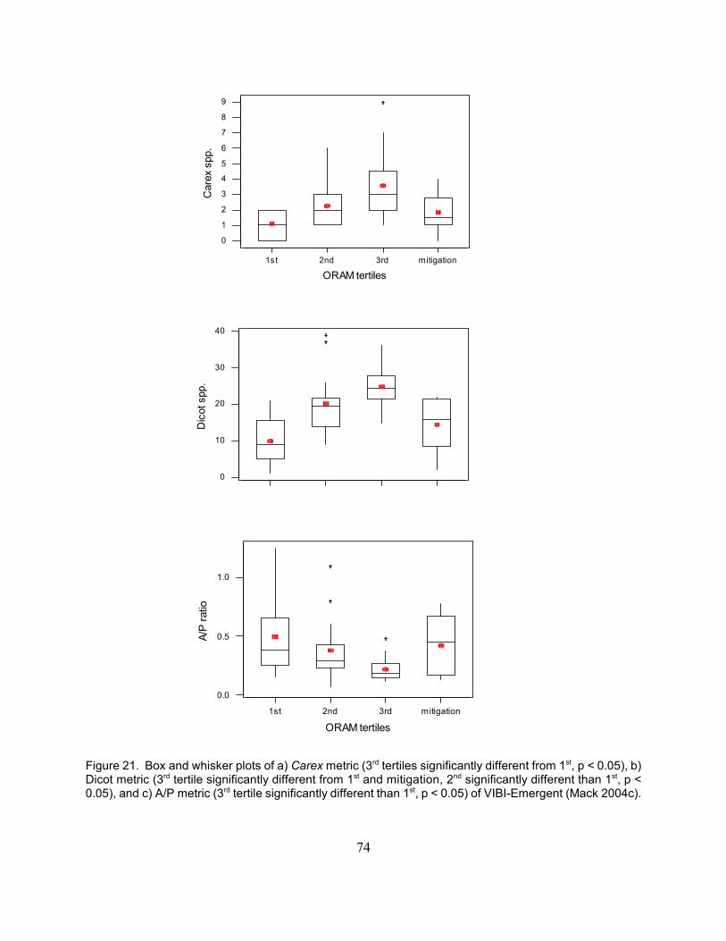
74

mitigation3rd2nd1st

40

30

20

10

0

ORAM tertiles

Dic

ot s

pp.

mitigation3rd2nd1st

1.0

0.5

0.0

ORAM tertiles

A/P

ratio

m itigation3rd2nd1st

9

8

7

6

5

4

3

2

1

0

ORAM tertiles

Car

ex s

pp.

Figure 21. Box and whisker plots of a) Carex metric (3rd tertiles significantly different from 1st, p < 0.05), b)Dicot metric (3rd tertile significantly different from 1st and mitigation, 2nd significantly different than 1st, p <0.05), and c) A/P metric (3rd tertile significantly different than 1st, p < 0.05) of VIBI-Emergent (Mack 2004c).

75

1st 2nd 3rd mitigation

0.00.1

0.20.30.40.5

0.60.70.8

0.91.0

ORAM tertiles

%un

vege

tate

d

mitigation3rd2nd1st

1500

1000

500

0

ORAM tertiles

avg

biom

ass

g/m

2

mitigation3rd2nd1st

8

7

6

5

4

3

2

1

0

ORAM tertiles

nativ

e w

etla

nd s

hrub

spp

.

Figure 22. Box and whisker plots of a) shrub metric (3rd tertile significantly different from 1st, 2nd, andmitigation, 2nd significantly different from mitigation, p < 0.05), b) average biomass metric (1st tertilesignificantly different from 3rd and mitigation, and c) %unvegetated metric (mitigation marginally significantlydifferent than natural wetlands, p < 0.06) of VIBI-Emergent (Mack 2004c).

76

mitigation3rd2nd1st

1.00.90.80.70.6

0.50.40.30.20.1

0.0

ORAM tertiles

%in

vasi

ve g

ram

inoi

ds

1st 2nd 3rd mitigation

0

10

20

30

ORAM tertiles

FQAI

sco

re

1st 2nd 3rd mitigation

0

10

20

30

40

50

ORAM tertiles

Hydr

ophy

te s

pp.

Figure 23. Box and whisker plots of a) hydrophyte metric (3rd tertiles significantly different from 1st , 2nd, andmitigation, 2nd different from 1st, p < 0.05), b) FQAI metric (all means significantly different, p < 0.05), andc) %invasive graminoids metric (1st tertile significantly different than 2nd, 3rd, and mitigation, p < 0.05) of VIBI-Emergent (Mack 2004c).

77

1st 2nd 3rd mitigation

0.0

0.1

0.2

0.3

0.4

0.5

0.6

0.7

0.8

0.9

ORAM tertiles

%se

nsitiv

e sp

ecie

s

1st 2nd 3rd mitigation

0.00.1

0.2

0.3

0.4

0.50.6

0.7

0.8

0.91.0

ORAM tertiles

%to

lera

nt s

peci

es

Figure 24. Box and whisker plots of a) %tolerant metric (3rd tertile significantly different from 1st , 2nd, andmitigation, p < 0.05), b) %sensitive metric (3rd tertile significantly different from 1st, p < 0.05) of VIBI-Emergent (Mack 2004c).

78

mitigation3rd2nd1st

100

90

80

70

6050

40

30

20

10

0

ORAM tertiles

VIBI

-E 2

004

Figure 25. Vegetation Index of Biotic Integrity scores (VIBI) (Mack 2004c). Box and whisker plots representORAM score tertiles (thirds). All means are significantly different (p < 0.05) except 1st tertile and mitigation.

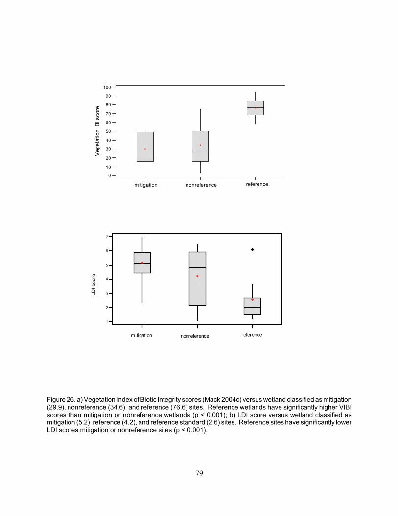
79

100

90

80

70

60

50

40

30

20

10

0

Veg

etat

ion

IBI s

core

mitigation nonreference reference

7

6

5

4

3

2

1

LDI s

core

mitigation nonreference reference

Figure 26. a) Vegetation Index of Biotic Integrity scores (Mack 2004c) versus wetland classified as mitigation(29.9), nonreference (34.6), and reference (76.6) sites. Reference wetlands have significantly higher VIBIscores than mitigation or nonreference wetlands (p < 0.001); b) LDI score versus wetland classified asmitigation (5.2), reference (4.2), and reference standard (2.6) sites. Reference sites have significantly lowerLDI scores mitigation or nonreference sites (p < 0.001).

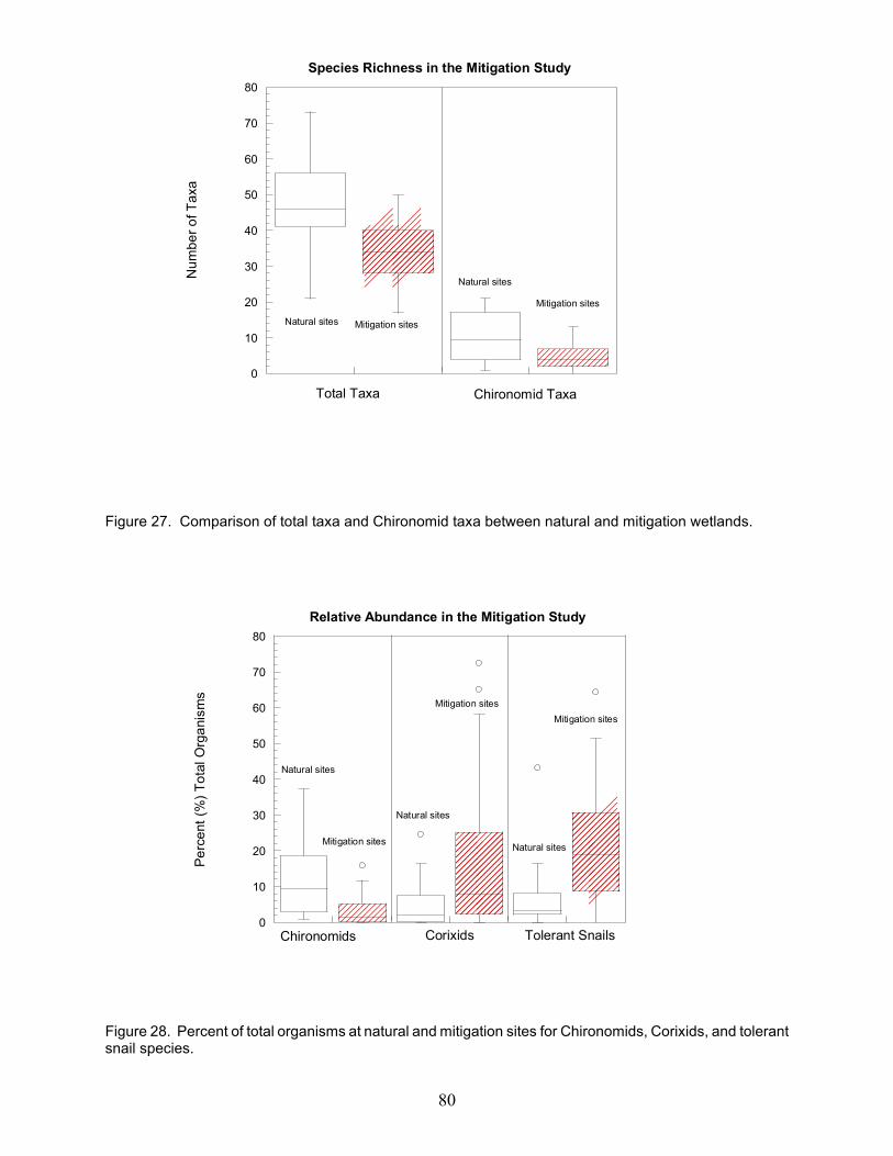
80

������������

���0

10

20

30

40

50

60

70

80Species Richness in the Mitigation Study

Num

ber o

f Tax

a

Natural sites

Total Taxa Chironomid Taxa

Natural sites

Mitigation sites

Mitigation sites

�� ��������

������������

0

10

20

30

40

50

60

70

80Relative Abundance in the Mitigation Study

Perc

ent (

%) T

otal

Org

anis

ms

Natural sites

CorixidsChironomids

Natural sites

Mitigation sites

Mitigation sites

Natural sites

Mitigation sites

Tolerant Snails

Figure 27. Comparison of total taxa and Chironomid taxa between natural and mitigation wetlands.

Figure 28. Percent of total organisms at natural and mitigation sites for Chironomids, Corixids, and tolerantsnail species.

81

��������������������

���������������

0

10

20

30

40

50

60

Mitigation Nonreference Reference

Wetland Invertebrate Community Index (WICI)

WIC

I Met

ric V

alue

s

n = 21 n = 68 n = 60

May to June/July samples (Julian > 120 days)

Figure 29. Wetland Invertebrate Community Index (WICI) scores for mitigation, nonreference and referencewetlands. n = number of sample events not number of sites.

82

Figure 30. Comparison of wetland trophic relationships between reference and nonreference (impacted)and mitigation wetlands.

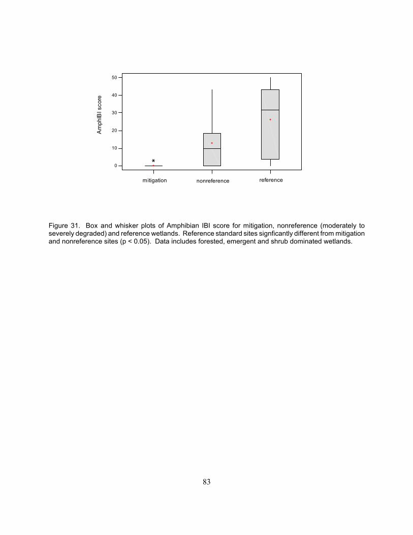
83

0

10

20

30

40

50

Am

phIB

I sco

re

mitigation nonreference reference

Figure 31. Box and whisker plots of Amphibian IBI score for mitigation, nonreference (moderately toseverely degraded) and reference wetlands. Reference standard sites signficantly different from mitigationand nonreference sites (p < 0.05). Data includes forested, emergent and shrub dominated wetlands.

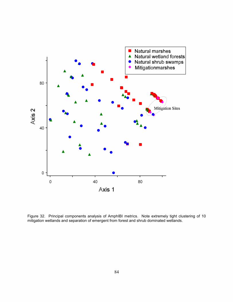
84

Figure 32. Principal components analysis of AmphIBI metrics. Note extremely tight clustering of 10mitigation wetlands and separation of emergent from forest and shrub dominated wetlands.

85

Figure 33. Detrended correspondence analysis of of amphibian presence and abundance. Total intertia(variance) in species data = 6.26, eigenvalues = 0.831, 0.658, 0.436, axes 1, 2, and 3, respectively. Noteeffect of wood frogs (RANSYL), spotted salamanders (AMBMAC), marbled salamander (AMBOPA) andjefferson salamanders (AMBJEFF) on ordination.

86

Figure 34. Detrended correspondence analysis of 8 natural and 10 mitigation wetlands. Total inertia(variance) in species data =3.19, eigenvalues = 0.766, 0.387, and 0.168, axes 1, 2, and 3 respectively.

87

0

20

40

60

80

100

120

0 58 109 321

Created Natural

p = 0.07p = 0.05 p = 0.05

% massremaining

Figure 35. Percent mass remaining of ON-SITE Typha over the study period. Each data point is the meanof 5 stations per site per collection period. Error bars are standard error.

0

20

40

60

80

100

120

0 58 109 321

Created Natural

p = 0.15 p = 0.02 p = 0.001

% massremaining

Figure 36. Percent mass remaining of CONTROL Typha over the study period. Each point is the mean of3 stations per collection period per site. Error bars are standard error.

88

1.5

2

2.5

3

3.5

0 50 100 150 200 250 300 350 400

Approximate Number of Days in Wetland

%N

Typ

ha l

itter

NaturalCreated

p=0.09p=0.009

nsd

p = 0.05

Figure 37. Nitrogen (%) in the ON-SITE Typha litter in each decomposition period. The value for each pointrepresents an average of 2 stations per site. Error bars represent the standard error.

89

0

0.05

0.1

0.15

0.2

0.25

0.3

0.35

0 50 100 150 200 250 300 350 400

Average Number of Days in Wetland

P ug

/g Ty

pha

litte

r

NaturalCreated

p = 0.001

p = 0.07

nsd nsd

Figure 38. Phosphorus concentrations (µg/g) in the ON-SITE Typha litter in each decomposition period.The value for each point represents an average of 2 stations per site. Error bars represent the standarderror.

90

1

1.5

2

2.5

3

3.5

4

0 50 100 150 200 250 300 350

Average Number of Days in Wetland

%N

Typ

ha li

tter

NaturalCreated

nsd p=0.05p=0.05

Figure 39. Total N (%) in the CONTROL Typha litter in each decomposition period. The value for each pointrepresents an average of 2 stations per site. Error bars represent the standard error.

91

0

0.05

0.1

0.15

0.2

0.25

0 50 100 150 200 250 300 350

Average Number of Days in Wetland

P ug

/g Ty

pha

litte

r

NaturalCreated

p = 0.01

p = 0.001

nsd

Figure 40. Phosphorus concentrations (µg/g) in the CONTROL Typha litter in each decomposition period.The value for each point represents an average of 2 stations per site. Error bars represent the standarderror.

92

����������������������������������������������������������������������������������������������������������������������������������������������������������������������������������������������������

������������������������������

��������������������������������������������������������������������������������������������������������� ���������������

���������������������������������������������������������������������������������������������������������������������������������������������������������������������������������������������������

����������������������������

�������������������������������������������������������� ��������������

0

0.5

1

1.5

2

2.5

3

3.5

4

%N %P g N/m2 g P/m2

������ Natural������ Mitigation

% o

r g

per m

2

Figure 41. a) Initial litter concentrations of N and P at the time of peak biomass and b) the resulting standingstocks of N and P (g/m2) in each wetland type. Differences were significant in each case (two sample t-testfor % concentrations p < 0.10, for standing stocks p < 0.05).

93

mitigation3rd2nd1st

1500

1000

500

0

ORAM tertiles

avg

biom

ass

g/m

2

Figure 42. The relationship between the wetland disturbance categories (ORAM tertiles) and mean biomassproduction (g/m2) in emergent marshes in Ohio. 1st tertile significantly different from 2nd, 3rd, and Mitigation(p < 0.05).

94

Figure 43. The relationship between FQAI scores and biomass production for the 19 wetlands included inthis study. Because the regression models were so different for the population of natural wetlandscompared to the population of mitigation sites, each is graphed separately. Both models are significant (p< 0.10), where Mitigation biomass = 82.2-4.3*FQAI (R2 = 0.30) and Natural biomass = 50.4 – 1.1*FQAI (R2

= 0.22).

95

0.02

0.03

0.04

0.05

0.06

0.07

0.08

deco

mpo

sitio

n (g

per

day

)

mitigation 3rd tertile2nd tertiles1st and

a.

0.02

0.03

0.04

0.05

0.06

0.07

0.08

deco

mpo

stio

n (g

per

day

)

mitigation natural

b.

Figure 44. Decomposition rates for ON-SITE litter after 2nd litter bag removal for a) wetland disturbancecategories (ORAM tertiles) (1st and 2nd ~ high to moderate disturbance), 3rd ~ low disturbance) and b) bywetland type (natural or mitigation). Line in 44a is line hand fitted to mean values.

96

30252015

7.0

6.5

6.0

5.5

TOC (mg/l), water

deco

mpo

sitio

n (g

)

25155

6.8

6.3

5.8

% Organic C, soil

deco

mpo

sitio

n (g

)

25155

6.8

6.3

5.8

% Organic C, soil

deco

mpo

sitio

n (g

)

Figure 45. The influence of total organic carbon (mg/L) in the water column on decomposition (total masslost in g at the 3rd pick-up) (R2 = 83.7%, p = 0.019) for 5 natural wetlands in this study. No water samplecollected at Rickenbacker because of early dry down in 2001. Eagle Cr Beaver, Eagle Cr Marsh, and LakeAbrams excluded due to possible inter-year differences.

Figure 46. The influence of percent organic carbon in the soil on decomposition (total mass lost in g at 3rd

pickup) (R2 = 63.1% p = 0.059) in 6 natural wetlands included in this study. Eagle Cr Beaver, Eagle CrMarsh, and Lake Abrams excluded due to possible inter-year differences.

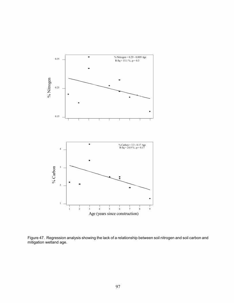
97

987654321

0.35

0.25

0.15

Age (years since construction)

% N

itrog

en

R-Sq = 15.1 % ; p = 0.3% Nitrogen = 0.29 - 0.009 Age

987654321

4

3

2

1

Age (years since construction)

% C

arbo

n

R-Sq = 24.9 % ; p = 0.17% Carbon = 3.3 - 0.17 Age

Figure 47. Regression analysis showing the lack of a relationship between soil nitrogen and soil carbon andmitigation wetland age.

98

Mitigation wetlands Natural wetlands

0

.005

.01

.015

.02

.025

.03

.035

Surface water present

Surface water absent k

Figure 48. Differences in decomposition rates in mitigation and natural wetlands as a function of waterpresence at the time of litterbag retrieval.

99

mitigationnonreferencereference

432

6.5

5.5

4.5

3.5

initial litter N content (mg N/g tissue)

mas

s lo

st g

@ 9

mon

ths

mitigationnonreferencereference

432

7

6

5

4

3

2

initial N content l i tter (mg N/g l itter)

mas

s lo

st g

@ 6

mon

ths

mitigationnonreferencereference

432

6.5

5.5

4.5

3.5

2.5

initial l i tter N content (mg N/g l itter)

mas

s lo

ss g

@ 3

mon

ths

Figure 49. On-site litter mass lost at approximately 3, 6 and 9 months versus initial litter N content (mg N/glitter) for mitigation, nonreference, and reference (least impacted) sites. Lines are fitted regression lines for3 months (p = 0.995, R2 = 0%), 6 months (p = 0.030, R2 = 31.4%), 9 months (p = 0.021, R2 = 34.7%).

100

Figure 50. Flow chart of nutrient dynamics in mitigation wetlands relative to natural ecosystems. Low nutrientavailability in wetland soils affects both biomass production and the plant litter nutrient concentration. Lowlitter nutrient concentrations negatively affects the decomposition rates, and slow decomposition rates alongwith low nutrient accumulation by litter limits the accumulation of nutrients in soil.

Soil Nitrogen Availability

Decomposition rate

(-)(-)

(-)

(-)

(-)

(-)

(-)

Soil N accumulation

Initial Soil Conditions

Tissue N concentration

Biomass Production

N release

101

2 5 4 8 3 9 12 13 11 16 1 7 6 10 15 17 14 18 19 100.00

80.62

61.25

41.87

Similarity

Wetland Sites

Figure 51. Cluster analysis using a combination of vegetation (FQAI score) and soil characteristics (% totalcarbon and % nitrogen). Natural wetlands outlined in box. Key for wetland sites: 1 = Sacks, 2 = Calamus,3 = Rickenbacker, 4 = Lodi North, 5 = Eagle Cr Beaver, 6 = Slate Run Bank SE, 7 = Medallion No. 20,8 = Ballfield, 9 = Dever, 10 = Bluebird, 11 = Baker Swamp 12 = Lake Abrams, 13 = New Albany HS, 14= Prairie Lane, 15 = Big Island Area D, 16 = Eagle Cr Marsh, 17 = JMB, 18 = Pizutti, 19 = Trotwood.

102

151314118910421265731

45.07

63.38

81.69

100.00

Similarity

Observations

Figure 52. Cluster analysis using the physiochemical variables (soil N and C) and plant litter Nconcentration. Natural wetlands outlined with box. Key for wetland sites: 1 = Calamus, 2 = Rickenbacker,3 = Lodi North, 4 = Ballfield, 5 = Dever, 6 = Baker Swamp, 7 = New Albany HS, 8 = Bluebird, 9 = BigIsland Area D, 10 = JMB, 11 = Pizzuitti, 12 = Sacks, 13 = Slate Run Bank SE, 14 = Medallion No. 20, 15= Prairie Lane.

103

Figure 53. Detrended correspondance analysis of of natural and mitigation wetlands (n = 19 sites, 110species, 13 environmental variables). Total inertial (variance) in species data = 6.66; eigenvalues = 0.851,0.795, and 0.744 for axes 1, 2, and 3 respectively. Biplot indicates distribution of sites relative to keyenvironmental variables. All mitigation wetlands ordinate in the left-center of the plot while natural sites aredispersed primarily to the right of the circle. One natural wetland is an exception, grouping closer to themitigation sites. This site is Dever which was the wetland most degraded by human activities (agriculture).The two natural sites circled on the right are reference standard sites.