Integrating Tomographically Improved Earth Structure Models Into Ground- Motion Simulations for Physics-based Seismic Hazard Analysis: Integration of

SCEC CME Computational Pathway 2 and 4

2010 Annual Report

Po Chen, Department of Geology and Geophysics, University of Wyoming Kim B. Olsen, Department of Geosciences, San Diego State University

1. Introduction In 2010, we submitted a proposal, titled “Integrating Tomographically Improved Earth Structure Models Into Ground- Motion Simulations for Physics-based Seismic Hazard Analysis: Integration of SCEC CME Computational Pathway 2 and 4”, to SCEC. The purpose of this proposal is to develop computational infrastructures to integrate Pathway 2 and 4 by delivering to the SCEC USR databases the tomographically derived structural perturbations as overlays on the starting models and incorporating those updated structure models into Pathway 2 simulations and quantifying the improvements and deficits of those updated models. We identified three scientific objectives:

A. Develop a standardized procedure for delivering tomographically derived structural perturbations to the SCEC simulation community as structural overlays onto the reference models.

B. Assess the quality of the updated structural models through a standardized set of measurements that quantify the misfit between observed seismograms and model-predicted seismograms.

C. Improve the parameterization of 3D structure in terms of seismic velocities, attenuation factors and anisotropy.

In the following, we will report the progresses we have made in reaching the three scientific objectives. 2. Task A The tomographically inverted model perturbations are usually defined on a mesh. In F3DT based on the finite-difference code, the mesh is uniform. In F3DT based on the spectral-element code, the grid spacing is heterogeneous and varies according to the S- wave speed in the reference model. As the reference model varies from iteration to iteration, the mesh, either uniform or heterogeneous, has to adapt to the minimum S-wave speed in the current reference model to ensure there are sufficient number of grid points within each wavelength and the CFL condition is satisfied. To transfer the model perturbations between different meshes, we need an interpolation/extrapolation rule. We have developed and tested an MPI-parallelized interpolation code, “pok”, based on the ordinary-kriging algorithm. Kriging is a group of geostatistical techniques for interpolating the value of a random field at an unobserved location from observations of its value at nearby locations. The kriging method is used widely in geology, mining, hydrology and other disciplines of geosciences. Ordinary kriging is the most commonly used type of kriging method. It assumes the random field is stationary and the number of observations is enough for estimating the variogram. Our C code for ordinary kriging has been parallelized using MPI and can perform interpolation for a large number of grid points used in wave-propagation simulations very efficiently. Recently, this code has been used in constructing a 3D starting model for finite-difference wave-propagaion simulations in Northern California. The 3D starting-model of P- and S-

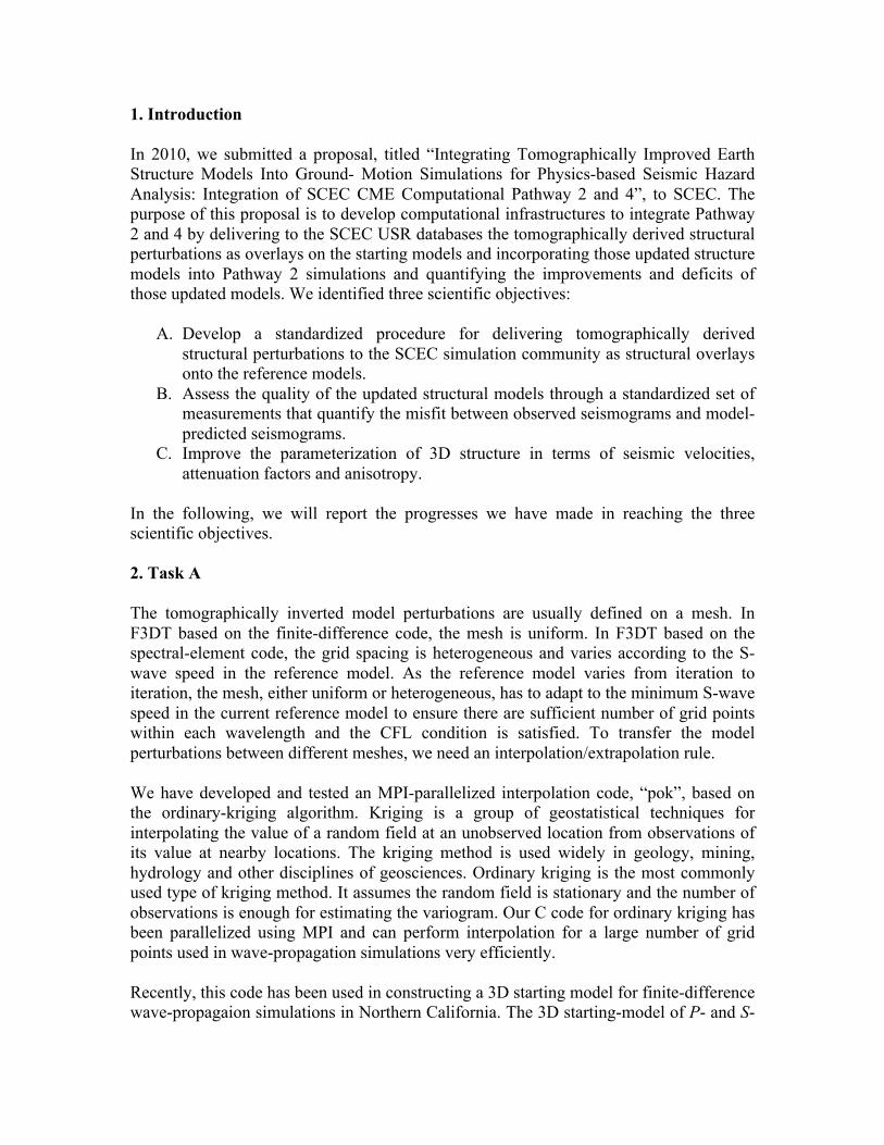
wave speeds for our study region in Northern California were constructed from a ray travel-time tomography model provided by Lin et al. (2010) (A California statewide three-dimensional seismic velocity model from both absolute and differential Times, BSSA 2010) using the “pok” code. Lin et al.’s Vp and Vs models, which are defined on an irregular mesh with grid-spacing varying from 1 km at shallower depths to 10 km at larger depths, are interpolated onto our finite-difference simulation mesh with 500-meter uniform grid spacing and full-3D wave-propagation simulations have been carried out using our interpolated 3D starting model and the 4th-order staggered-grid finite-difference code, AWP-ODC. The synthetic seismograms provide satisfactory fit to the observed P- and S-wave first-arrival travel-times. A comparison of the Vp and Vs models at 1 km depth before and after the interpolation are shown in Figure 1. 3. Task B Full-3D waveform tomography (F3DT) requires a criterion to quantify the fit between observed waveforms and their corresponding synthetic waveforms. This misfit criterion is used in defining the objective function of the F3DT and also provides a quantitative measure for the quality of the updated structure models. We have adopted the goodness-of-fit (GOF) criterion, which includes a set of user-weighted metrics such as peak ground motions, response spectrum, the Fourier spectrum, cross correlation, and energy release measures, in our F3DT procedure to evaluate the quality of tomographically updated structure models. So far, we have completed two iterations of F3DT for Southern California. GOF measures were calculated to evaluate the quality of each updated structure model. These measures are generally consistent with the misfit measurements

Figure 1. Lin et al.’s ray travel-time tomography models (left column) and the interpolated models used in our full-3D finite-difference wave propagation simulations (right column) for both Vp (upper row) and Vs (lower row). The mapviews shown here are for Vp and Vs models at 1 km depth.

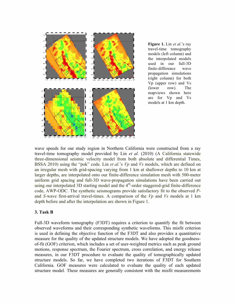
used in our F3DT inversion procedure, which is the generalized seismological data functionals (GSDF). Histograms of the GOF distribution for the starting model CVM4, the two tomographically updated structure models, CVM4SI1 and CVM4SI2, are shown in Figure 2.

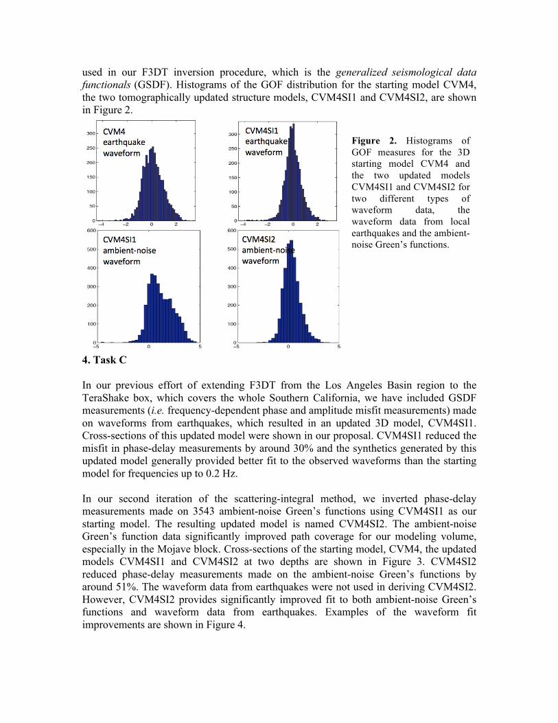
4. Task C In our previous effort of extending F3DT from the Los Angeles Basin region to the TeraShake box, which covers the whole Southern California, we have included GSDF measurements (i.e. frequency-dependent phase and amplitude misfit measurements) made on waveforms from earthquakes, which resulted in an updated 3D model, CVM4SI1. Cross-sections of this updated model were shown in our proposal. CVM4SI1 reduced the misfit in phase-delay measurements by around 30% and the synthetics generated by this updated model generally provided better fit to the observed waveforms than the starting model for frequencies up to 0.2 Hz. In our second iteration of the scattering-integral method, we inverted phase-delay measurements made on 3543 ambient-noise Green’s functions using CVM4SI1 as our starting model. The resulting updated model is named CVM4SI2. The ambient-noise Green’s function data significantly improved path coverage for our modeling volume, especially in the Mojave block. Cross-sections of the starting model, CVM4, the updated models CVM4SI1 and CVM4SI2 at two depths are shown in Figure 3. CVM4SI2 reduced phase-delay measurements made on the ambient-noise Green’s functions by around 51%. The waveform data from earthquakes were not used in deriving CVM4SI2. However, CVM4SI2 provides significantly improved fit to both ambient-noise Green’s functions and waveform data from earthquakes. Examples of the waveform fit improvements are shown in Figure 4.

Figure 2. Histograms of GOF measures for the 3D starting model CVM4 and the two updated models CVM4SI1 and CVM4SI2 for two different types of waveform data, the waveform data from local earthquakes and the ambient-noise Green’s functions.

Figure 3. Cross-sections of the starting model CVM4 and the perturbations after the first and the second F3DT iterations. Plotted are the Vs model and Vs perturbations at 2.5 km and 5.5 km depths.

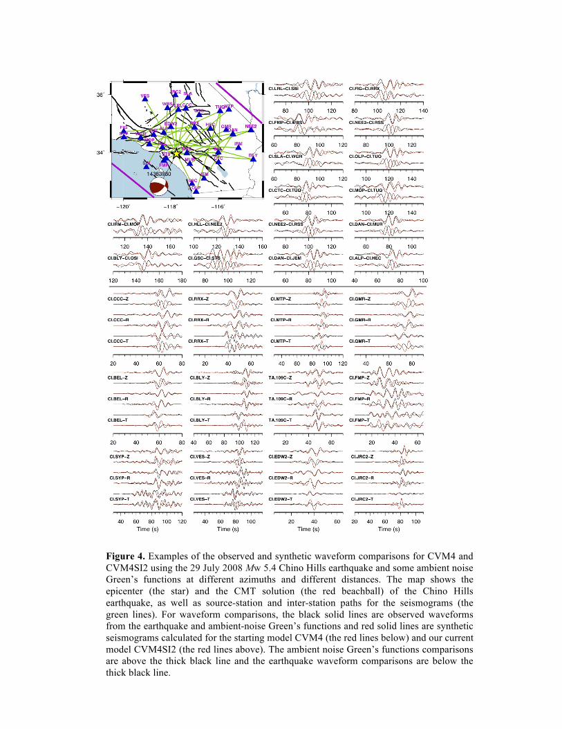
Figure 4. Examples of the observed and synthetic waveform comparisons for CVM4 and CVM4SI2 using the 29 July 2008 Mw 5.4 Chino Hills earthquake and some ambient noise Green’s functions at different azimuths and different distances. The map shows the epicenter (the star) and the CMT solution (the red beachball) of the Chino Hills earthquake, as well as source-station and inter-station paths for the seismograms (the green lines). For waveform comparisons, the black solid lines are observed waveforms from the earthquake and ambient-noise Green’s functions and red solid lines are synthetic seismograms calculated for the starting model CVM4 (the red lines below) and our current model CVM4SI2 (the red lines above). The ambient noise Green’s functions comparisons are above the thick black line and the earthquake waveform comparisons are below the thick black line.