Embed Size (px)
Citation preview

Integration of Bridge Damage Detection Concepts and Components
Final Report 3 of 3October 2013
Sponsored byIowa Highway Research Board(IHRB Project TR-636)Iowa Department of Transportation(InTrans Project 11-416)
Volume III: Wireless Bridge Monitoring Hardware

About the BEC
The mission of the Bridge Engineering Center is to conduct research on bridge technologies to help bridge designers/owners design, build, and maintain long-lasting bridges.
Disclaimer Notice
The contents of this report reflect the views of the authors, who are responsible for the facts and the accuracy of the information presented herein. The opinions, findings and conclusions expressed in this publication are those of the authors and not necessarily those of the sponsors.
The sponsors assume no liability for the contents or use of the information contained in this document. This report does not constitute a standard, specification, or regulation.
The sponsors do not endorse products or manufacturers. Trademarks or manufacturers’ names appear in this report only because they are considered essential to the objective of the document.
Non-Discrimination Statement
Iowa’s Regent Universities do not discriminate on the basis of race, color, age, religion, national origin, sexual orientation, gender identity, genetic information, sex, marital status, disability, or status as a U.S. veteran. Inquiries can be directed to the Iowa State University Director of Equal Opportunity and Compliance, 3280 Beardshear Hall, (515) 294-7612.
Iowa Department of Transportation Statements
Federal and state laws prohibit employment and/or public accommodation discrimination on the basis of age, color, creed, disability, gender identity, national origin, pregnancy, race, religion, sex, sexual orientation or veteran’s status. If you believe you have been discriminated against, please contact the Iowa Civil Rights Commission at 800-457-4416 or Iowa Department of Transportation’s affirmative action officer. If you need accommodations because of a disability to access the Iowa Department of Transportation’s services, contact the agency’s affirmative action officer at 800-262-0003.
The preparation of this report was financed in part through funds provided by the Iowa Department of Transportation through its “Second Revised Agreement for the Management of Research Conducted by Iowa State University for the Iowa Department of Transportation” and its amendments.
The opinions, findings, and conclusions expressed in this publication are those of the authors and not necessarily those of the Iowa Department of Transportation.

Technical Report Documentation Page
1. Report No. 2. Government Accession No. 3. Recipient’s Catalog No.
IHRB Project TR-636
4. Title and Subtitle 5. Report Date
Integration of Bridge Damage Detection Concepts and Components
Volume III: Wireless Bridge Monitoring Hardware
October 2013
6. Performing Organization Code
7. Author(s) 8. Performing Organization Report No.
Jin Zhu InTrans Project 11-416
9. Performing Organization Name and Address 10. Work Unit No. (TRAIS)
Electrical Engineering Technology
University of Northern Iowa
Cedar Falls, IA 50614
11. Contract or Grant No.
12. Sponsoring Organization Name and Address 13. Type of Report and Period Covered
Iowa Highway Research Board
Iowa Department of Transportation
800 Lincoln Way
Ames, IA 50010
Final Report 3 of 3
14. Sponsoring Agency Code
IHRB Project TR-636
15. Supplementary Notes
Visit intrans.iastate.edu for color pdfs of this and other research reports.
16. Abstract
In this work, a previously developed structural health monitoring (SHM) system was advanced toward a ready-for-implementation
system. Improvements were made with respect to automated data reduction/analysis, data acquisition hardware, sensor types, and
communication network architecture.
This report volume (Volume III) summarizes the energy harvesting techniques and prototype development for a bridge monitoring
system that uses wireless sensors. The wireless sensor nodes are used to collect strain measurements at critical locations on a
bridge. The bridge monitoring hardware system consists of a base station and multiple self-powered wireless sensor nodes. The
base station is responsible for the synchronization of data sampling on all nodes and data aggregation. Each wireless sensor node
include a sensing element, a processing and wireless communication module, and an energy harvesting module.
The hardware prototype for a wireless bridge monitoring system was developed and tested on the US 30 Bridge over the South
Skunk River in Ames, Iowa. The functions and performance of the developed system, including strain data, energy harvesting
capacity, and wireless transmission quality, were studied and are covered in this volume.
17. Key Words 18. Distribution Statement
energy harvesting—monitoring hardware—prototype—SHM—structural
health monitoring—wireless sensors
No restrictions.
19. Security Classification (of
this report)
20. Security Classification (of this
page)
21. No. of Pages 22. Price
Unclassified. Unclassified. 75 NA
Form DOT F 1700.7 (8-72) Reproduction of completed page authorized

THREE-VOLUME REPORT ABSTRACT
The Iowa Department of Transportation (DOT) started investing in research (through both the
Iowa Highway Research Board and the Office of Bridges and Structures) in 2003 to develop a
structural health monitoring (SHM) system capable of identifying damage and able to report on
the general operational condition of bridges. In some cases, the precipitous for these
developments has been a desire to avoid damage that might go unnoticed until the next biennial
inspection. Of specific and immediate concern was the state’s inventory of fracture-critical
structures.
The goal of this project was to bring together various components of recently-completed research
at Iowa’s Regent Universities with the following specific objectives:
Final development of the overall SHM system hardware and software
Integration of vibration-based measurements into current damage-detection algorithm
Evaluation and development of energy-harvesting techniques
The following three volumes of the final report cover the results of this project:
Volume I: Strain-Based Damage Detection, from the Iowa State University Bridge
Engineering Center, reviews information important to the strain-based SHM methodologies,
details the upgraded damage-detection hardware and software system, demonstrates the
application of the control-chart-based methodologies developed, and summarizes the results in
graphical and tabular formats.
Volume II: Acceleration-Based Damage Detection, from the University of Iowa Center for
Computer-Aided Design, presents the use of vibration-based damage-detection approaches as
local methods to quantify damage at critical areas in structures. Acceleration data were collected
and analyzed to evaluate the relationships between sensors and with changes in environmental
conditions. A sacrificial specimen was investigated to verify the damage-detection capabilities
and this volume presents a transmissibility concept and damage-detection algorithm that show
potential to sense local changes in the dynamic stiffness between points across a joint of a real
structure.
Volume III: Wireless Bridge Monitoring Hardware, from the University of Northern Iowa,
Electrical Engineering Technology, summarizes the energy harvesting techniques and prototype
development for a bridge monitoring system that uses wireless sensors. The functions and
performance of the developed system, including strain data, energy harvesting capacity, and
wireless transmission quality, are covered in this volume.

INTEGRATION OF BRIDGE DAMAGE DETECTION
CONCEPTS AND COMPONENTS
VOLUME III: WIRELESS BRIDGE MONITORING
HARDWARE
Final Report 3 of 3
October 2013
Principal Investigator
Brent M. Phares, Director
Bridge Engineering Center, Iowa State University
Co-Principal Investigators
Salam Rahmatalla, Associate Professor
Civil and Environmental Engineering, Center for Computer-Aided Design, University of Iowa
Jin Zhu, Associate Professor
Electrical Engineering Technology, University of Northern Iowa
Ping Lu, Rating Engineer
Office of Bridges and Structures, Iowa Department of Transportation
Research Assistants
Bekir Yuksek, Ranjana Joshi, Laura Hattaway, Sultan Altamimi
Author
Jin Zhu
Sponsored by
the Iowa Highway Research Board and Iowa Department of Transportation
(IHRB Project TR-636)
Preparation of this report was financed in part
through funds provided by the Iowa Department of Transportation
through its Research Management Agreement with the
Institute for Transportation
(InTrans Project 11-416)
A report from
Electrical Engineering Technology
University of Northern Iowa
Cedar Falls, IA 50614
Phone: 319-273-2597


v
TABLE OF CONTENTS
ACKNOWLEDGMENTS ............................................................................................................. ix
EXECUTIVE SUMMARY ........................................................................................................... xi
1. INTRODUCTION .......................................................................................................................1
1.1 Background and Motivation ..........................................................................................1 1.2 Research Scope and Objectives .....................................................................................2 1.3 Proposed Wireless Bridge Monitoring System ..............................................................2 1.4 Report Content ...............................................................................................................3
2. LITERATURE REVIEW ............................................................................................................4
2.1 Wireless Sensor Networks for Structure Monitoring.....................................................4
2.2 Energy Harvesting Techniques for WSNs .....................................................................5
2.3 Energy Storage and Power Management .....................................................................12
3. WIRELESS BRIDGE MONITORING HARDWARE SELECTION AND DESIGN .............16
3.1 Overview ......................................................................................................................16 3.2 Wireless Sensor Platform for Bridge Monitoring ........................................................17
3.3 Energy Harvesting Component ....................................................................................22 3.4 Energy Storage Component .........................................................................................26
3.5 Energy Harvesting and Storage Circuit Design ...........................................................32
4. FIELD TESTS AND PERFORMANCE EVALUATION ........................................................35
4.1 Field Test Configuration ..............................................................................................35
4.2 Strain Data Analysis ....................................................................................................40
4.3 Energy Harvesting and Self-Sustainability Evaluation................................................47 4.4 Wireless Transmission Quality Analysis .....................................................................51
5. SUMMARY AND CONCLUSIONS ........................................................................................55
REFERENCES ..............................................................................................................................59

vi
LIST OF FIGURES
Figure 1. Self-powered wireless sensor node ................................................................................16 Figure 2. MicroStrain wireless sensor network platform ...............................................................19 Figure 3. SG-Link-LXRS power profile (Vcc = 5V) .....................................................................20
Figure 4. SG-Link node in synchronous burst mode .....................................................................22 Figure 5. Power-voltage (P-V) curve of the solar panel PowerFilm P7.2-75 ................................24 Figure 6. Power-voltage (P-V) curve of 4 Sanyo 8801 solar panels in parallel ............................24 Figure 7. Maximum power points at different light levels ............................................................25 Figure 8. PowerFilm WeatherPro solar panel (P7.2-75)................................................................25
Figure 9. Power consumption of SG-Link node in synchronous burst mode ................................27 Figure 10. Total energy needed per day for the operation in synchronous mode with 128 Hz
sample rate .........................................................................................................................28
Figure 11. Super-capacitor stored energy versus usable energy (350 F) .......................................29 Figure 12. Capacitance demand for given energy level for 24 hour operation ..............................30 Figure 13. Charge distribution and leakage effects of super-capacitors: (a) voltage changes
over 48 hours (b) energy loss as a percentage of the initial energy ...................................31 Figure 14. EHSuperCap board schematic and PCB layout............................................................33
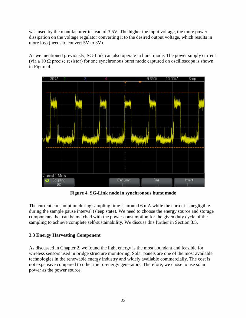
Figure 15. Node prototype .............................................................................................................34 Figure 16. US 30 Bridge over the South Skunk River ...................................................................36 Figure 17. Wireless sensor node locations on US 30 Bridge .........................................................37
Figure 18. Weldable strain gauge ..................................................................................................37 Figure 19. Solar panels (a) performance test (b) attached on the bridge (south side) ...................38
Figure 20. Wireless sensor node installed on the bridge ...............................................................39 Figure 21. Strain plot of four sensor nodes over 24 hours .............................................................41 Figure 22. Raw data baseline for small segment ...........................................................................43
Figure 23. Frequency response ......................................................................................................44
Figure 24. Zeroed and filtered strain data ......................................................................................44 Figure 25. Filtered strain data for four nodes ................................................................................45 Figure 26. Three 30 second segments of filtered strain data for Node 649 and Node 712............46
Figure 27. Positive and negative peaks ..........................................................................................47 Figure 28. Sample capacitor voltage records .................................................................................48
Figure 29. Temperature data versus voltage gain ..........................................................................50 Figure 30. Energy level gain/loss in Node 651 ..............................................................................51
Figure 31. Node RSSI and Base RSSI ...........................................................................................53

vii
LIST OF TABLES
Table 1. Comparison of energy sources .........................................................................................11 Table 2. Energy density of rechargeable battery chemistries (Roundy et al. 2004) ......................12 Table 3. Performance comparison between ultra-capacitor and lithium-ion battery .....................14
Table 4. Comparison of energy storage components .....................................................................14 Table 5. Requirements of wireless sensor node platform compared with microstrain SG-Link
nodes ..................................................................................................................................18 Table 6. Average current consumption of SG-Link (1 channel active, continuous mode, Vcc =
3.5V) ..................................................................................................................................21
Table 7. Average current consumption of SG-Link (3 channel active, continuous mode, Vcc =
3.5V) ..................................................................................................................................21 Table 8. Light levels at various weather conditions ......................................................................23
Table 9. Super-capacitor specifications .........................................................................................32 Table 10. Configurations of synchronized SG-Link-LXRS sampling nodes ................................35 Table 11. Light intensity level measured in the solar panel location .............................................50


ix
ACKNOWLEDGMENTS
The authors would like to thank the Iowa Highway Research Board (IHRB) and Iowa
Department of Transportation (DOT) for sponsoring this research. The authors are grateful to the
technical advisory committee (TAC) members for their thoughtful discussions and input. Special
thanks to Alexander M. Boechler for his support and help for performing field tests. The authors
would also like to acknowledge the administrative support of the Department of Technology at
the University of Northern Iowa.


xi
EXECUTIVE SUMMARY
This report is divided into three volumes.
This volume (Volume III) summarizes the energy harvesting techniques and prototype
development for a bridge monitoring system that uses wireless sensors. The wireless sensor
nodes are used to collect strain measurements at critical locations on a bridge. The bridge
monitoring hardware system consists of a base station and multiple self-powered wireless sensor
nodes. The base station is responsible for the synchronization of data sampling on all nodes and
data aggregation. Each wireless sensor node include a sensing element, a processing and wireless
communication module, and an energy harvesting module.
The hardware prototype of a wireless bridge monitoring system was developed and tested on the
US 30 Bridge over the South Skunk River in Ames, Iowa. The functions and performance of the
developed system, including strain data, energy harvesting capacity, and wireless transmission
quality, were studied.


1
1. INTRODUCTION
Structure monitoring is traditionally performed through periodic visual inspections. Although
structural health monitoring (SHM) has been an important tool for evaluating structures for
several decades, it has only been within the last decade that specific effort has been given to
developing wireless monitoring that does not need to run cables all over the bridge for easy and
fast installation and improved flexibility.
In addition, a wireless monitoring system that can harvest energy from the ambient environment
has gained attention in recent years because a self-powered system eliminates the maintenance
requirement for battery changes.
1.1 Background and Motivation
According to data from the Federal Highway Administration (FHWA), nearly 25 percent of all
bridges are deficient nationally as of December 2012 (FHWA 2012). For Iowa, the deficiency
rate was 26.4 percent, including 5,193 bridges that were structurally deficient and 1,282 bridges
that were functionally obsolete, in 2009. Therefore, the development of an automatic and low-
cost bridge SHM system is in high demand and crucial to reduce the costs associated with
manual inspection, to effectively monitor the status of bridges, and to, therefore, prevent
collapses in bridge infrastructures.
Following the projects completed by the Iowa State University Bridge Engineering Center on
bridge performance by applying long-term SHM systems in 2003 and 2006 (Wipf et al. 2006 and
2007), a project at the University of Northern Iowa, completed in 2010, sought to evaluate the
feasibility of using wireless sensor systems for transportation system monitoring (Salim and Zhu
2010). Because a significant cost of any bridge monitoring system is in the cost of cabling and its
installation, this work is of great importance to the widespread use of bridge monitoring.
However, one major drawback of the system is battery-powered wireless sensor nodes. The
battery lifetime is limited and replacing the batteries can become an expensive and tedious task,
or it’s impractical for most of scenarios. The limited energy storage remains a major technical
challenge that hinders the widespread deployment of wireless bridge monitoring systems, despite
the many advantages of using them for structure monitoring.
Therefore, it would be very attractive for wireless sensor nodes to obtain energy automatically
from the environment to power the sensing, processing, and communications operations to
thereby achieve complete self-sustainability. The process that converts energy in the ambient
environment into usable electrical power is called energy harvesting or energy scavenging.
Energy harvesting from the ambient environment has the potential to provide an alternative cost-
effective solution to the power requirement of wireless sensor networks for bridge monitoring.

2
1.2 Research Scope and Objectives
In this part of the research project, we focus on Objective 3: Evaluation and development of a
wireless bridge monitoring system with energy harvesting techniques. We evaluated various
energy sources from the ambient environment and their harvesting techniques for the outdoor
bridge monitoring environment in Iowa. The ambient energy sources include vibration, light, air
flow, heat, temperature variations, and ambient radio frequency (RF) energy. Literature reviews
have been completed to evaluate different energy harvesting techniques and ambient energy
resources for infrastructure from the aspects of availability, power density, and implementation
cost.
Although the energy resource is renewable for harvesting, it usually has its limitations. Wireless
sensor nodes must be designed as energy-efficiently as possible to achieve self-sustainability.
The energy conversion should be efficient and the loss during the conversion should be
minimized with the consideration of cost efficiency. It is important to select low-power feasible
devices. In addition, the implementation of effective power management and energy-aware
communication protocols can further improve the energy efficiency.
The wireless bridge monitoring system developed has been tested on the US Highway 30 (US
30) Bridge over the South Skunk River in Ames, Iowa to measure the strain data generated by
the ambient traffic across the bridge. The validation of the strain data and raw data process for
further data processing were studied. The self-sustainability of energy harvesting and reliability
of the wireless communication in the system were also analyzed.
1.3 Proposed Wireless Bridge Monitoring System
The proposed wireless bridge monitoring system is used to measure strains that result from
ambient traffic crossing the bridge at multiple locations under the bridge. Strain has been
selected based on the research recommendations from previous research (Wipf et al. 2006).
Weldable strain gauges have been considered as the best choice for short-term studies of steel
bridges. Testing has generally been carried out using normal traffic, with information on the
truck traffic to be extracted for structural health analysis (DeWolf 2009). The weldable strain
gauge R-leadwire series from Vishay Micro-Measurement are utilized. These gauges are
designed for long-term outdoor use. Mainly used in applications such as railroad and civil
structures, they can be exposed to oil and water splash (Vishay 2013).
The system that was developed was deployed for field tests and data collection on the US 30
Bridge. The demonstration bridge has a 30 ft wide roadway that supports two eastbound traffic
lanes. The posted speed limit is 65 miles per hour (mph) (105 kilometers per hour (kph)) (Wipf
et al. 2006). Four wireless sensing nodes with strain gauges were deployed on the west end of the
bridge. Along with the strain data, the power supply voltage, temperature measurements, and
wireless received signal strength indication (RSSI) were also collected periodically for analysis.

3
1.4 Report Content
The remainder of the report is organized as follows. Related works in wireless bridge monitoring
hardware design and energy harvesting are reviewed in Chapter 2. The procedures that selected
the technology and components for the developed system are discussed in Chapter 3. Presented
in Chapter 4 are the implemented hardware and field tests along with the data analysis. Chapter 5
summarizes the conclusions and provides recommendations for further research on wireless
bridge monitoring.

4
2. LITERATURE REVIEW
This chapter provides a general overview of the wireless sensor networks for bridge monitoring.
Specifically, the energy harvesting and storage techniques that have the potential in the wireless
bridge monitoring system are discussed.
2.1 Wireless Sensor Networks for Structure Monitoring
Wireless sensor networks (WSNs) have drawn a great deal of attention recently because of their
advantages and numerous potential applications. Their usage in SHM has been investigated by
Paek et al. (2005) and Chintalapudi et al. (2006). Banks et al. (2009) at Missouri University of
Science and Technology developed a low-cost wireless system that generates and sends road
safety alerts to motorist’s smart phones. Many of the systems developed are based on common
wireless sensor platforms, such as IMote and Mica (Mechitov et al. 2006, Rice and Spencer
2008, Pakzad et al. 2008, and Jo et al. 2011).
The most commonly-used sensors for the study of the wireless sensor networks in structure
monitoring are accelerometers and strain gauges. The traditional strain gauge and small-sized
semiconductor accelerometers are easy to interface with small sensor nodes and to deploy on site
conveniently.
Some wireless sensor boards used with common wireless sensor platforms and dedicated
wireless sensor platforms have been developed for SHM applications. Wang et al. (2007)
implemented a system with multithreaded sensing devices. Researchers at North Carolina State
University developed a wireless sensor node with strain gauges (Joshi et al. 2006). A Wireless
Intelligent Sensor and Actuator Network (WISAN) was developed to provide ultra-lower power
consumption (Sazonov et al. 2006). In addition, underground structure monitoring using wireless
sensor networks has been studied by Li and Liu (2007). A network of wireless sensors was used
for short-term monitoring on the Yeondae Bridge (Korea) to measure the global response of the
bridge to controlled truck loadings (Kim et al. 2010). A bridge structure monitoring system has
been developed using a ubiquitous WSN that has been installed on the Second Jindo Bridge in
Korea along with a cabled system to validate the WSN as a multi-national collaboration project
(Jo et al. 2011).
Synchronization is an important issue in collecting data from multiple sensors collaboratively,
especially for applications with high sampling frequency. In research completed by the
University of Illinois at Urbana-Champaign, a post-sensing time synchronization scheme was
proposed to achieve high accuracy of synchronization of collected data while reducing the
latency introduced by synchronization (Li et al. 2012). Other research has been done to utilize
global positioning system (GPS) signals for wireless sensor synchronization (Kim 2012). The
drawbacks of the GPS signal method include high power consumption and requirements for an
unobstructed view of the sky.
Most recently, the energy harvesting-enabled wireless sensor networks have drawn extra interest
from researchers. The researchers Musiani, Lin, and Rosing (2007) at the University of

5
California-San Diego presented a wireless sensing platform that combines localized processing
with energy harvesting to provide long-lived bridge monitoring. Wu and Zhou (2011) proposed a
new ultra-low power WSN structure to monitor the vibration properties of civil structures with
integrated energy harvesting, data sensing, and wireless communication. However, the structure
was only analyzed using simulations and still far from practical implementation. Researchers at
Clarkson University demonstrated a complete self-powered system utilizing energy harvested
from bridge vibrations (Sazonov et al. 2009). Another proposed approach is that a mobile host
(such as an unmanned aerial vehicle) charges the sensor nodes by wireless power delivery and
subsequently retrieves the data by wireless interrogation (Mascarenas et al. 2009). We review the
research work on energy harvesting techniques in the next section in detail.
2.2 Energy Harvesting Techniques for WSNs
As mentioned previously, one of the challenges that WSNs pose is the energy efficiency and
power supply problem. The wireless sensor nodes are in general battery-powered for easy
installation and re-deployment, getting rid of cables. If the batteries need to be changed
frequently, the deployment of a large-scale wireless sensor network is impractical, if not
impossible. The solutions to this challenge are two-fold: 1) minimize the power consumption of
the wireless sensor nodes, and 2) harvest energy from the ambient environment.
The first part can be achieved by adopting ultra-low power consumption integrated circuit (IC)
chips and developing energy-efficiency schemes and protocols for saving power. The second
part is particularly attractive if the nodes can achieve completely self-sustaining abilities by
harvesting energy, which may eventually eliminate battery changes. Accordingly, energy
harvesting is an area of rapid development. Companies, such as Linear Technology, Texas
Instruments, Pizeo Systems, and MicroStrain, are also starting to provide different
developmental tools or ICs for energy harvesting and power management in a small-scale energy
harvester.
Although renewable energy technology, such as solar panels and wind turbines, are relatively
mature, they are generally for large-scale systems and not suitable to low-cost, small-sized
wireless sensor nodes. Some pioneer projects have been undertaken to investigate the
possibilities of harvesting energy from the ambient environment for low-cost, micro wireless
sensors for SHM (Park 2008). The potential ambient energy sources that may be used for bridge
monitoring include vibration, light, air flow, temperature variations, and ambient RF energy. We
review each of the possible ambient energy sources and related works in the area in the following
subsections.
2.2.1 Vibration Energy Harvesting
Vibrations and acoustic noise are abundant in highway bridges and overpasses due to the traffic.
Those usually unfavorable vibrations may be utilized as a potential energy source. There are
multiple ways to transform vibrational energy into usable energy. The energy can be scavenged
by exploiting the oscillation of a proof mass tuned to the environment’s dominant mechanical
frequency. The damping force of the oscillation can be converted into electrical energy via

6
electromagnetic mechanism, electrostatic mechanism, or a piezoelectric mechanism (Mateu and
Moll 2005 and Roundy et al. 2004) as explained briefly as follows:
Electromagnetic energy harvesting: This technique uses a magnetic field to convert
mechanical energy to electrical energy based on Faraday’s law. It is limited by size
constraints as well as material properties.
Electrostatic energy harvesting: This method relies on the capacitance change of vibration-
dependent variable capacitors. The most attractive feature of this method is its ease to
integrate in ICs, given that micro-electromechanical systems (MEMS) variable capacitors
can be fabricated through relatively mature silicon micro-machining processes. This scheme
produces higher and more practical output voltage levels than the electromagnetic method,
with moderate power density. The disadvantage is a separate voltage source is required that
increases the practical difficulties.
Piezoelectric energy harvesting: This method converts mechanical energy to electrical
energy by applying strain to a piezoelectric material. When certain crystals are stretched or
compressed, charges appear on their surfaces. The voltage produced varies with time and
strain, effectively producing an irregular alternating current (AC) signal. The challenge is to
obtain piezoelectric materials with large enough piezoelectric coefficients to produce
relatively high voltage and power density level under strain.
The biggest challenge for finding an appropriate vibration energy harvester is to find one that
works efficiently in the presence of low, inconsistent frequencies that are consistent with the
motions of a bridge. This area has received great attention recently and various energy
scavenging materials and devices from vibration are under development.
Each of the vibration harvesting methods have their pros and cons. Due to the fact that current
electrostatic generators can only produce a lower-level energy, even from high excitation
frequencies, piezoelectric and electromagnetic methods have been studied in most work.
The majority of the previous work in electromagnetic generators focuses on high levels of
vibration energy (2.5to 10 ms-2
) or typical resonant frequencies of 100 hertz (Hz) or higher
(Beeby et al. 2006). Some recent work is concerned with the low level of vibration energy at a
lower frequency (100 Hz or lower). Beeby et al. (2006) reported an output of 4 milliwatts (4mW)
at 35 Hz using a novel electromagnetic method.
A wider European project called VIBES funded by the European Union further exploited
vibration energy scavenging solutions for wireless sensors (Torah et al. 2007). In this project, the
electromagnetic microgenerator used tungsten masses and neodymium (NdFeB) magnets on the
end of a cantilever beam structure combined with a stationary coil to harvest energy from
ambient vibrations. The generator used a 2300 turn coil using 12μm thick copper wire to achieve
a small size. The original test was done on an air compressor. The sensor node developed was
able to send back one sample every 50 seconds when the miniature electromagnetic vibration

7
energy harvester operated at resonances between 43 and 109 Hz at a modest vibration level of
0.6ms-2
. Although it is a significant improvement for lower frequencies, the resonance frequency
was still too high compared to bridge vibrations.
One noticeable work, completed by researchers at Clarkson University, developed a sensor node
to harvest energy from passing traffic using an electromagnetic generator on a girder (Sazonov et
al. 2009). A vibrating spring mass-electromagnetic system was developed and tuned to the
natural frequency of the bridge (3.1 Hz). The system developed was tested on a State Route 11
bridge in Potsdam, New York. The system demonstrated the possibility of utilizing vibration
energy to power wireless sensors. The drawback of the system was that no more than 500
samples could be collected per day per sensor node given the limited energy harvested from
vibrations due to passing traffic.
Researchers from the University of Michigan-Ann Arbor recently developed another system for
bridge vibrations with low acceleration (0.1 to 1 ms-2
) and variable frequency characteristics (1
to 40 Hz) (Galchev et al. 2011). Field test results showed consistent operation along the length of
the bridge, producing 0.46 to 0.72 microwatts (µW) of continuous (average) power (peaks in the
range of 30 to 100 µW), independent of the location of the harvester on the bridge and without
any modifications or tuning.
Electromagnetic coils can take up a lot of space, while piezoelectric materials are normally small
and thin (Mateu and Moll 2005). Because we would typically like the energy harvester to be
small along with the micro sensor nodes, research work in piezoelectric materials and its energy
harvester became popular. The most common type of piezoelectric material used is the
monolithic piezoceramic material.
In a study completed by Sodano et al. (2005), three types of piezoelectric materials used to
harvest ambient vibration energy were studied for comparison of their abilities to recharge
batteries. These included monolithic piezoceramic material, lead-zirconate-titanate (PZT), Micro
Fiber Composite (MFC), and bimorph Quick Pack (QP) actuator. The researchers’ findings were
that the MFC was not adequate at either resonant or random (0 to 500 Hz) frequencies to produce
enough power (large voltage, extremely low current) to charge a battery. The QP performed very
well at its resonant frequency, with an efficiency of about 8.9 percent, but performed poorly at
random frequencies, having an efficiency of only 0.45 percent. The PZT performed overall the
best, averaging around 1 to 2 percent at resonant and 3.9 percent efficient at random frequencies
from 0 to 500 Hz.
One issue that is faced when using piezoelectric materials to charge a battery is that the signal
must be converted to direct current (DC). A simple converter can be built by connecting a
voltage rectifier to a capacitor, and connecting the battery in parallel with the capacitor. This is
done to simplify the circuit as much as possible to reduce any voltage losses due to extra devices.
Some companies offer kits that provide the needed converting circuitry, but this adds cost and
may use up too much energy to be useful.

8
Given that the output of a piezoelectric generator is at an unregularly high amplitude AC, it has
to be converted to a given DC voltage for wireless sensors. Significant work has been published
on how to improve the power efficiency of control and converter circuits of piezoelectric
harvesters (Shen et al. 2010, Tabesh and Fréchette 2008, Aktakka et al. 2011, and Anton 2011).
Another issue with piezoelectric crystal vibrational harvesters is that they work best at certain
frequencies. When searching for piezoelectric materials, some companies offer ones that are
tuned. Tuning can be achieved by adding wax or some other small weight to the end of the
cantilever. Tuning the harvesters by hand is a tedious task of adding weight to the end until the
output voltage of the crystal is the maximum at the desired frequency. Each individual
vibrational harvester works best in a certain limited range of frequencies, and is usually more
efficient in higher frequencies. Bridges are large objects and therefore have low frequencies. A
more applicable use for these types of vibrational ambient energy harvesters might be to use
them in conjunction with industrial machines (Beeby et al. 2006).
Although research has made progress in this area, it can be seen that the vibration energy source
density is low and cannot provide sufficient energy for continuous monitoring with high
sampling rates, such as that for strains. Therefore, vibration harvesters are suitable to power the
sensor nodes in applications with a lower sample rate requirement, such as bridge environment
monitoring (temperature, water level, etc.) or event-triggered transmission in low frequency.
2.2.2 Wind or Air Flow Energy Harvesting
Wind or air flow energy has been used for centuries as a power source dating back to windmills.
As one of the most common renewable energy sources, wind energy harvesting has been widely
researched for high power applications where large wind turbine generators on wind farms are
used to supply power (Chen et al. 2009). The wind energy generated on wind farms are
connected to power grids. In Iowa, about 30 percent of the state’s electricity generation was
coming from wind in May 2013 (U.S. Energy Information Administration 2013).
The wind turbine generator needs to be miniaturized in size and highly portable to work with
micro-sized sensor nodes. Only a few research works have been done to study the issue of small-
scale wind energy harvesting using micro turbine generators (Tan and Panda 2011). By utilizing
the motion of an anemometer shaft to turn a compact generator, small amounts of power can be
harvested. The developed micro turbine (with 3 in. axial plates to house the rotor and stator) can
output more than 100 µW with a wind speed of 12 mph (Weimer et al. 2006). Park and Chou
(2006) developed an energy harvester, AmbiMax, that integrates both wind energy and solar
energy harvesting. The system was tested with Eco wireless sensor nodes to demonstrate its
functionality over 14 hours.
Although the small size of the energy harvesting module limits the generable power density, the
constant small air flow can be expected under bridges and therefore is also a potential energy
source for WSNs in bridge monitoring.

9
2.2.3 Solar Energy Harvesting
Solar energy is also one of the most common renewable energy sources. Photovoltaic (solar)
cells are becoming less expensive and more efficient with time. There are also more types of
solar cells now than ever before. The cells vary in size, as well as chemical and physical makeup.
The most common types are made from crystalline silicon and differ mainly in the way they are
produced. These different production techniques separate the cells into categories including
monocrystal, polycrystal, amorphous (also called thin film), and multijuction (or multi-layered)
panels. Most of the information is known about the semiconductor silicon, but additional
research is being done with the thickness, spacing, and chemical additives to the silicon layers.
Similar to wind energy, the research on solar energy is concerned primarily with high-power
applications. For example, Oozeki studied the performance trends in grid-connected photovoltaic
systems for public and industrial use (Oozeki et al. 2010).
One of the research concentrations surrounds developing new materials and structures to
improve solar cell efficiency and efficiency has continued to improve over the past few years.
The recent Solar Cell Efficiency Table published by John Wiley & Sons reported the new record
for energy conversion efficiency for any photovoltaic converter under one sun (the global air
mass AM1.5 spectrum with 1,000 W/m2) is an efficiency of 37.9 percent for a 1 cm
2 indium
gallium phosphide/gallium arsenide/indium gallium arsenide (InGaP/GaAs/InGaAs) monolithic
multijunction cell fabricated by Sharp (Green et al. 2013). The main problem with most solar
cells is that they are mostly on or off: the cell either produces a voltage difference, when the
photons of the sun are energetic and numerous enough, or it does not, and there is very little
middle ground. Research work on WSNs with low power level solar energy harvesting mostly
focuses on outdoor environments.
Some solar energy harvesters for wireless sensors have been developed (Park et al. 2006, Taneja
et al. 2008, and Brunelli et al. 2009) and modeling and design issues are discussed in the research
work by Raghunathan et al. (2005), Dondi et al. (2008), and Alippi and Galperti (2008). Solar
energy has been a popular selection as the renewable energy source for wireless bridge
monitoring systems (Nordblom and Galbreath 2012). Some work for indoor applications under
low light environments has also been conducted (Gorlatova et al. 2010).
An Energy Harvesting Active Networked Tag (EnHANT) prototype has been developed based
on a MICA2 mote and includes a custom-designed sensor board with a light sensor and a solar
cell with the purpose to provide self-powered networked RF tags. Solar cells that perform better
in lower light can be useful to power under-the-bridge sensors.
2.2.4 RF Energy Harvesting
With the increased popularity of wireless communication devices, we might consider
background radio signals as a potential energy reservoir. However, ambient radiation sources

10
have extremely limited power and an RF energy harvester generally requires either a large
collection area or very close proximity to the radiating source (such as a transmitter tower)
(Paradiso and Starner 2005).
In the research work by Bouchouicha et al. (2010), RF energy harvesting devices were studied
and the surrounding RF power density was measured. The average of the total radiation power
density in broadband (1gigahertz (GHz) to 3.5GHz) is in the order of 63μW/m2. The maximum
of the RF density power, approximately 40 μW/m2, is measured in the 1.8 GHz to 1.9 GHz
frequency band on which wireless cellular phones work. Multiple antennas have been designed
to recover the ambient RF energy and the best performance is obtained with a spiral antenna. The
maximum harvested DC power is around 0.1 μW in outdoor ambient, near a mobile phone base
station.
Because of its extremely lower energy density, RF energy harvesting is not suitable for
applications that require continuous monitoring or high sampling rates.
2.2.5 Thermal Energy Harvesting
The temperature difference in objects or environment can be converted to electricity via heat
transfer. Due to the Seebeck effect, a temperature difference between the junctions of a loop of
material consisting of at least two dissimilar conductors leads to an electromotive force (emf)
and, consequently, an electric current. Thereby, a thermocouple or thermopile can be used as a
thermoelectric generator based on the theory.
When exposed to temperature gradients, the emf produced in a thermocouple is proportional to
the temperature difference between the hot and cold junctions. Efficient thermoelectric
generators should be made of thermoelectric materials possessing a large Seebeck coefficient, a
low electrical resistivity, and a low thermal conductivity, and some fairly recent research is
concerned with improved thermoelectric generator design with novel materials (Strasser et al.
2003). However, the efficiency is limited.
Carnot efficiency provides the fundamental limit to the energy obtained from a temperature
difference. In the case of the temperature difference between the human body and the room
temperature (20C), Starner estimates that the maximum efficiency with this condition is 5.5
percent (Paradiso and Starner 2005). Energy conversion using thermopile arrays can only attain
efficiencies below 20 percent for a temperature difference of 500C (from 800 Kelvin to 300
Kelvin), below 10 percent for a temperature difference of 150C, and below 1 percent for a
temperature difference of 20C (Rowe 2006).
Recent research shows that the power density of a thermoelectric generator is good, with 8 W/kg
for a temperature difference of 10 Kelvin for Eureca TEG1-9.1-9.9-0.8/200 and, therefore,
thermoelectric generators are suitable to harvest energy in aircrafts because of the lightweight
requirement for aircraft applications (Becker et al. 2008).

11
Dalola et al. developed a temperature system that utilizes a thermoelectric module to power
sensor RF transmission when it is placed on a heat source (Dalola et al. 2008). The result showed
that for a temperature gradient of 8C the maximum readout distance was about 0.91 in. (23
mm).
Recent research demonstrated energy harvest from pavement structures by exploiting the thermal
gradient between the pavement base and subgrade (Wu and Yu 2012). The results showed that
with a temperature difference of 20C, the system was able to drive a light-emitting diode (LED)
periodically.
From the above reviews, thermoelectric generators are suitable for environments with high
thermal gradients, such as a hot exhaust pipe or a heat radiator, but not suitable for bridge
monitoring environment given that the temperature gradient is small for bridge surfaces.
2.2.6 Comparison of Ambient Energy Sources
Although many different techniques are available to harvest energy from ambient environments
to power wireless sensors, the amount of available raw energy with permitted surface area or net
mass limit the total power yield. A comparison of the energy sources is provided in Table 1.
Table 1. Comparison of energy sources
Source Type
Harvesting Performance
(Power Density) Reference
Vibration/Motion
Human motion
Industry machines
Bridge vibration due to
passing traffic
4 μW/cm2
100 to 800 μW/cm2
< 1 μW/cm3
Paradiso and Starner 2005
Raju and Grazier 2010
Galchev et al. 2011
Acoustic Noise 0.003 μW/cm3 at 75 dB
0.96 μW/cm3 at 100 dB
Park et al. 2008
Temperature Difference
Human
Industry
25 μW/cm2
1 to 10 mW/cm2
Raju and Grazier 2010
Wind/Air Flow 380 μW/cm2 (assumes air velocity of
5 m/s, i.e., 11 mph)
Roundy et al. 2004
Solar/Light
Indoor
Outdoor
7.2 μW/cm2 (office light)
100 mW/cm2 (directed toward bright sun)
10 mW/cm2 (under sun)
150 μW/cm2 (cloudy)
Roundy et al. 2004
Paradiso and Starner 2005
Raju and Grazier 2010
Park et al. 2008
RF
GSM
WiFi
Broadband (1 - 3.5GHz)
0.1 μW/cm2
0.001 μW/cm2
0.0063μW/cm2
Raju and Grazier 2010
Bouchouicha et al. 2010

12
The data show that most available power is at μW/cm2 levels, except the solar cells under bright
sunlight. Because the wireless bridge monitoring sensors are required to operate in outdoor
environments, solar energy is the most promising source. Specifically, we are looking for small-
scale cells that can be used for medium- to low-light situations given that sensors may be placed
where direct sunlight is not guaranteed.
2.3 Energy Storage and Power Management
An energy harvesting module consists of charger circuits, energy storage components, and
voltage regulators. The energy harvested from the ambient environment needs to be stored in
some energy storage components, such as the following:
Electrochemical batteries
Micro-fuel cells
Ultra-capacitors or super-capacitors
Micro-heat engines
Batteries are the most common energy storage devices. Rechargeable batteries can be used with
energy harvesters in WSNs. The energy density of a few common rechargeable battery types is
given in Table 2. Among them, lithium rechargeable batteries have the desirable features of high
energy density and durability.
Table 2. Energy density of rechargeable battery chemistries (Roundy et al. 2004)
Chemistry Lithium NiMHd NiCd
Energy Density (J/cm3
) 1080 860 650
Besides batteries, fuel cells are potentially very attractive for WSNs because of their high energy
density. For example, methanol has an energy density of 17.6 kilojoules per cubic centimeter
(kJ/cm3), which is more than 10 times that of lithium-ion batteries. Micro-sized fuel cells that
have similar sizes as cellphone batteries are not available yet commercially, but prototypes have
been made.
Two drawbacks of fuel cells are slow start-up and high cost. Perhaps more importantly, a high
temperature is needed to obtain high efficiencies. At higher temperatures, conversion times
decrease (Park et al. 2008). The typical operating temperature range is 0 to 200°C (Schaevitz
2012) and, therefore, is not suitable for bridge monitoring applications in Iowa where
temperatures may easily drop below zero.
Multiple research groups have also undertaken the development of various micro-heat engine-
based power generation approaches. Some on-going micro-engine projects include micro gas
turbine engines, Rankine steam turbines, free and spring-loaded piston internal combustion
engines, and thermal-expansion-actuated piezoelectric power generators (Park et al. 2008). The

13
expected benefits of micro-heat engines are their high power density and high density energy
storage. However, most projects are in early stages of development and performance has not
been well demonstrated.
The utilization of super-capacitors in WSNs has drawn some attention recently. Brunelli et al.
(2009) and Kim et al. (2011) developed and investigated the super-capacitor charging circuits for
wireless sensor nodes. Super-capacitors (also known as ultra-capacitors or double-layer
capacitors) can have a very high capacitance value, ranging from several Farads to 3,000 Farads.
Ultra-capacitors can be considered as a compromise of rechargeable batteries and standard
capacitors. Super-capacitors achieve significantly higher energy density than standard capacitors,
but retain many of the favorable characteristics of capacitors, such as long life and short charging
time. The typical voltage of super-capacitors is confined to 2.5 volts (2.5V) to 2.7V.
Super-capacitors store charge in an electric double layer to increase their effective capacitance.
They have an ultra-low internal resistance and the initial equivalent series resistance (ESR) is
typically in the level of milliohms (mΩ).
Super-capacitor lifetime is affected predominantly by a combination of operating voltage and
operating temperature. The super-capacitor has an unlimited shelf life when stored in a
discharged state. When referring to lifetime, the manufacturer data sheets usually reflect the
change in performance, typically a decrease in capacitance and increase in ESR. To give one
example, a 15 percent reduction in rated capacitance and a 40 percent increase in rated resistance
may occur for a super-capacitor held at 2.5V after 88,000 hrs (10 years) at 25C (Maxwell
Technologies 2012).
The lifetime of rechargeable batteries is much shorter. A test on a commonly-used lithium-
ion/lithium cobalt oxide (LiCoO2) cell showed that a fully-charged cell kept at 25°C
permanently lost 20 percent of total capacity after one year. The cycle life of super-capacitors,
ranging from 500,000 to 1 million, is also superior compared to the cycle life of rechargeable
batteries.
Although super-capacitors have many advantages, the energy density of commercially-available
super-capacitors is about one order of magnitude higher than standard capacitors and about one
to two orders of magnitude lower than rechargeable batteries (or about 50 to 100 J/cm3) (Park et
al. 2008). A detailed performance comparison between ultra-capacitors and lithium-ion
rechargeable batteries is shown in Table 3 (Cadex Electronics 2013).

14
Table 3. Performance comparison between ultra-capacitor and lithium-ion battery
Ultra-capacitor Lithium-ion
Type Electrostatic Electrochemical
Charge time 1–10 seconds 10 to 60 minutes
Cycle life 300,000 - 1 million Over 500
Cell voltage 2.3 to 2.75V 3.6 to 3.7V
Specific energy (Wh/kg) 5 (typical) 100 to 200
Specific power (W/kg) Up to 10,000 1,000 to 3,000
Energy Management Cell over voltage Cell equalization
Charge/Discharge Abuse and rapid discharge tolerant Sensitive to rapid charge/discharge
Cost per Wh $20 (typical) $2.8 to $5 (typical)
Service life 10 to 15 years 2 to 6 years
Charge temperature -40 to 65°C (-40 to 149°F) 0 to 45°C (32° to 113°F)
Discharge temperature -40 to 65°C (-40 to 149°F) -20 to 60°C (-4 to 140°F)
The operating temperature for super-capacitors is wider than that for lithium-ion batteries,
especially for charging. This wider operating temperature range is a good fit to the outdoor
weather in Iowa. In addition, one of the issues of WSNs with rechargeable batteries for long-
term monitoring is the limited lifetime and cycle life. Therefore, super-capacitors could be an
attractive option in some wireless sensor node applications because of their increased lifetimes,
short charging times, high power densities, and wide operating temperature ranges.
The overall comparison of different energy storage components is given in Table 4.
Table 4. Comparison of energy storage components
Type
Energy
Density
(J/cm3)
Power
Density
(μW/cm3)
1 yr lifetime
Power
Density
(μW/cm3)
10 yr lifetime
Secondary
Storage
Needed?
Commercially
Available?
Non-rechargeable
battery (lithium)
3500 45(a)
3.5(a)
No Yes
Rechargeable battery
(lithium-ion)
1080 7(a) 0(a) - Yes
Mirco-fuel cell
(methanol)
5040(b) 280(a) 28(a) Maybe No
Ultra-capacitor
50-100(a) 5100-7400c 3500-5500(c) No Yes
Heat engine 3346(d) 106(d) - Yes No
a. Park et al. 2008
b. Mobion product information from MTI MicroFuel Cells Inc.
c. 2013 ultra-capacitor data sheets from Maxwell Technologies (assume mass-to-volume ratio 1.2 kg/l)
d. Roundy et al. 2004
Efficient power management is important to maximize the benefits of the harvested energy in
addition to selecting the proper energy source and energy reservoir. Most of the efforts have

15
proposed using energy harvesting to charge on-board batteries or super-capacitors. While
harvesting technology provides the ability to scavenge energy from the ambient environment, the
scavenged energy shows the characteristic of irregular, random, intermittent and low-energy
bursts due to the changing environment.
In addition, harvesting components and energy storage elements usually have different voltage-
current characteristics. Therefore, efficient charging and power management circuits must be
integrated with the system to minimize the conversion loss and translate the scavenged energy to
increase system lifetime.
Communication and processing modules require a stable supply power and, therefore, a highly-
efficient voltage regulator is indispensable. For better reliability, multiple energy sources need to
be considered to complement each other (Park and Chou 2006).
For solar cells, significant work has been done on power electronic circuit design to provide
maximum power point tracking (MPPT) because the current versus voltage (I-V) characteristics
of photovoltaic modules change non-linearly when the irradiance condition changes. Most of the
work is for large-scale solar power systems.
Fairly recent work by Park and Chou (2006), Brunelli et al. (2008), Simjee and Chou (2006), and
Alippi and Galpertic (2008) exploited the low-power systems of MPPT. Either a microcontroller
or analog circuits are used to track the peak power point. Given that, at low-power levels, the
tradeoffs between the MPPT implementation and the overhead to implement MPPT need to be
considered carefully. Raghunathan et al. (2005) made efforts to enable near-perpetual operations
of low-power embedded systems by implementing harvesting-aware operations by matching the
source and storage, without implementing MMPT.

16
3. WIRELESS BRIDGE MONITORING HARDWARE SELECTION AND DESIGN
3.1 Overview
In this chapter, we provide the information on evaluation and hardware design of the components
for a wireless bridge monitoring system. The system includes one data collector center or base
station and multiple wireless sensor nodes. A wireless sensor node consists of four main
components: power module, processing module, communication module, and sensing module.
Figure 1 provides a conceptual diagram of a self-powered wireless sensor node.
Figure 1. Self-powered wireless sensor node
Given that commercially-available wireless sensor nodes typically include both processing and
wireless communication modules, we needed to select an appropriate platform to tailor it to the
requirements of the bridge monitoring application. We also developed an energy harvesting
module that works with the selected wireless sensor platform to achieve self-sustainability.
Although the energy source for harvesting is renewable, it is still very limited and each node
must be as energy-efficient as possible to achieve self-sustainability. We obtained the energy
consumption profiles for the selected wireless sensor platform, LORD MicroStrain Sensing
Systems’ SG-Link, when it was used to monitor the strain condition. Based on the obtained
results, we carefully selected energy source and storage components, designed the power
management circuit, and tried to optimize the operation so that each node can achieve complete
self-sustainability by harvesting energy from the ambient environment.
Energy Harvesting Module light, vibration, wind, temp.
Sensing
elements
Processor RF
Transceiver
Memory Storage
Micro-scale
generator
Charging
circuit
Energy
storage
Voltage
regulator
ADC
Wireless Sensor Platform

17
3.2 Wireless Sensor Platform for Bridge Monitoring
Various wireless sensor hardware platforms have been developed, led by the development of
mote nodes at the University of California-Berkeley in the late 1990s. One detailed comparison
of the wireless sensor nodes can be found in the work by Lynch and Loh (2006).
A number of commercial wireless sensor platforms are available that may be suited for SHM
use. Because a commercial wireless sensor system can provide easy operation and technical
support and also cost less, we considered using one of these general wireless sensor platforms
instead of developing one from scratch.
One of the commonly-used platforms in academia is the mote wireless sensor platform
developed initially at Berkeley and commercialized by Crossbow Technology, Inc. Mote
wireless sensor node platforms include MICA2, MICAz, IRIS, TelosB, and Intel Mote2 (Imote2)
(xbow.com). Other platforms include Tmote from Sentilla (popular in academia, but support
discontinued), XBee from Digi International (digi.com), Ember ZigBee (acquired by Silicon Lab
in 2012, silabs.com), and MicroStrain (acquired by LORD in 2012, microstrain.com).
Wireless communication is considered the major part of the power consumption for sensor
nodes. Wireless communication technologies that are available for WSNs include IEEE 802.11
standard (wireless fidelity-wireless internet/Wi-Fi), Bluetooth, ultra-wide band (UWB), ZigBee
or Institute of Electrical and Electronics Engineers (IEEE) 802.15.4 standard, wireless universal
serial bus (USB), infrared (IR) wireless, and radio frequency identification (RFID), etc. Each of
these standards is accompanied by advantages and limitations, as discussed in previous work
(Salim and Zhu 2010). IEEE 802.15.4 standard-compliant transceivers, working in 2.4 GHz
industrial, scientific and medical (ISM) band are popular for WSN platforms because they
addresses the low-power implementation for a large-scale wireless network with low data rate
monitoring and a control application where the data rate is less than 250 kbps where low cost and
complexity is desired. For a larger transmission range, transceivers that work in 868 MHz and
900 MHz are also commonly adopted.
Besides the wireless sensor platforms mentioned above, several wireless-compatible data
acquisition nodes or data loggers designed to work with strain gauges are also available
commercially including Wireless Strain Gauge Solutions (scanimetrics.com), SENSeOR
(senseor.com/), CWB100 and CWS900 (campbellsci.com/wireless), and Wireless Data Logger
(geokon.com/wireless-datalogger/). However, most of these do not support point-to-multipoint
synchronized data sampling.
3.2.1 Application Requirements
Before we selected the wireless sensor node platform, the specific requirements for our bridge
monitoring application were identified. According to objectives of the project, the sensing
elements used are traditional strain gauges and the system needs to monitor the bridge strain
peaks due to live passing traffic.

18
Based on previous research (Lu 2008), it is suggested that the 125 Hz data acquisition frequency
is adequate to capture strain peaks produced by highway-speed trucks. In addition,
synchronization of sampling data from multiple sensor nodes is necessary to ensure the accuracy
of the engineering analyses performed on the response data. Considering that the error
introduced due to synchronization error should be no greater than 1 percent, the synchronization
error should be less than 80 µs.
With a total bridge span of 320 ft (97.5 m), the transmission range of the wireless sensor nodes
must be 328.08 ft (100 m) or more. The platform should also support point-to-multipoint or mesh
communication given that multiple strain gauges are needed for synchronized strain monitoring.
Assuming a measurement range of ±500 µstrain with 1 µstrain resolution, at least a 10 bit
analog-to-digital converter (ADC) is needed. In addition, the sensor nodes should be able to
provide excitation to the Wheatstone bridge for strain gauges. Given that we need to use an
energy harvester to power the sensor node, the platform should provide an interface for the
external power supply. The platform needs to be operated outdoors and, therefore, a wide
operating temperature range is expected.
Based on the requirements, after comparing multiple different nodes, we selected SG-Link nodes
from LORD MicroStrain Sensing Systems (microstrain.com). MicroStrain started to develop and
provide wireless sensor network systems for strain monitoring in the late 1990s (Arms 2004). In
addition to an SG-Link node satisfying the requirements, it has a communication module that is
IEEE 802.15.4 standard compliant and a free software development kit (SDK) is provided.
Sample code in C++, LabVIEW and Visual Basic (VB.Net) are also provided. SDK can be used
for development of our own application software based on the application needs. The required
features for the monitoring task and features of SG-Link nodes are compared in Table 5.
Table 5. Requirements of wireless sensor node platform compared with microstrain SG-
Link nodes
Required Features MicroStrain SG-Link Specifications
Data sample rate ≥ 125 Hz Up to 4 kHz
1Hz - 512Hz for synchronous mode
ADC resolution > 10-bit 12 bit
Synchronization between nodes < 80 µs ±32 µsecond, synchronous sample rate stability ±3ppm
Transmission distance > 100 m Up to 2 km for outdoor open space
Analog inputs: at least 1 differential
and 1 single ended
1 differential input channel,1 single-ended input channel
with 0 to 3 volt excitation, and an internal temperature
sensor channel
Communication: support point-to-
multipoint or mesh
Support point-to-multipoint
Operating temperature: -40C to +50C -20C to +60C with the internal lithium-ion battery
-40C to +85C for electronics
Lower power consumption Data logging 25mA, sleeping 100 µA
Support external power supply Yes

19
In this project, we used four SG-Link-LXRS nodes with extended transmission range for
demonstration and tests. A SG-Link node weighs 50 g and is very compact, as shown in Figure
2(a). The base station used is WSDA-Base-104, as shown in Figure 2(b), which can interface
with a computer via USB port. Another option is to use WSDA-Base-1000, as shown in Figure
2(c), that supports Ethernet connections and thus is able to transmit data to the internet if an
internet connection is available via cable or a cellular network adapter.
(a ) SG-Link-LXRS node (b) WSDA-Base-104
(c) WSDA-Base-1000
Figure 2. MicroStrain wireless sensor network platform
3.2.2 Operation Modes
SG-Link-LXRS node has a differential input channel (strain channel), a single-ended input
channel (analog channel), and an on-board temperature sensor channel. The differential channel
is excited with 3 volts and the input is first passed through two-stage amplification and then into
a 12 bit analog to digital converter (ADC). The data can be sampled in four different modes:
datalogging, low-duty cycle (LDC), streaming, and synchronous.
Datalogging stores in the 2 megabyte on-board memory can be finite or continuous or event-
triggered. When configured as event-triggered, the node will not automatically go into sleep
mode. The LDC mode can be configured to work at very low frequency (from 500 Hz to 1
sample/hr) and the node will transmit the data back to the base when the base is enabled to
collect data. Streaming allows the data to be transmitted back to node at a high sampling rate;

20
however, only one sensor node can communicate to the base simultaneously. Synchronous
sampling mode was a new feature introduced in version 7. In synchronous mode, the base sends
1Hz beacons to synchronize all the nodes within the network. The supported sample rates in
synchronous mode are from 1Hz to 512Hz. Synchronous mode supports both continuous and
burst sampling. In this project, based on the application requirements, we used synchronous
mode with a sample rate of 128 Hz.
3.2.3 Power Profile
Before selecting the energy harvesting and storage circuit, SG-Link-LXRS was first tested to
obtain its power consumption profile. It was necessary for appropriate energy source selection to
provide enough energy while not over designing it. The power profile was obtained from the
manufacturer, as shown in Figure 3.
(Available at files.microstrain.com/SG-Link-LXRS-Power-Profile.pdf)
Figure 3. SG-Link-LXRS power profile (Vcc = 5V)
With 3V excitation voltage, we can expect the increased current consumption for 350 Ohms (Ω)
over 1000Ω to be 5.57 milliamperes (mA). The actual measurement results are slightly higher
than this calculation, ranging from 5.83 mA to 6.93 mA.

21
There is not information here on the power consumption for three active channels or on the other
operation modes. We also wanted to know if the power consumption would increase if more than
one node is in the network (i.e., possibly more communication overhead). Therefore, we
performed some tests for different scenarios and the results are shown in Table 6 and Table 7.
Table 6. Average current consumption of SG-Link (1 channel active, continuous mode, Vcc
= 3.5V)
Sample Rate
# of nodes
128 Hz 256 Hz 512 Hz
LDC
mode
1 0.015A 0.036A 0.045A
2 0.016A 0.038A -
Sync.
normal
1 0.006A 0.008A 0.011A
2 0.006A 0.008A 0.011A
Sync.
High
capacity
1 0.005A 0.007A 0.011A
2 0.005A 0.007A 0.011A
Table 7. Average current consumption of SG-Link (3 channel active, continuous mode, Vcc
= 3.5V)
Sample Rate
# of nodes
128 Hz 256 Hz 512 Hz
LDC
mode
1 0.016A 0.038A 0.048A
2 0.016A 0.038A -
Sync
normal
1 0.008A 0.011A 0.018A
2 0.007A 0.011A -
Sync.
High
capacity
1 0.008A 0.011A 0.018A
2 0.007A 0.011A -
Notice the results are for scenarios that used 1000 Ω strain gauges. It can be seen that
synchronous mode consumes much less power than the LDC mode. It can also be seen when
three channels are active, the power consumption increases. The results we obtained are slightly
lower than the results from the manufacturer power profile. The reason is that a 5V power supply
22
was used by the manufacturer instead of 3.5V. The higher the input voltage, the more power
dissipation on the voltage regulator converting it to the desired output voltage, which results in
more loss (needs to convert 5V to 3V).
As we mentioned previously, SG-Link can also operate in burst mode. The power supply current
(via a 10 Ω precise resistor) for one synchronous burst mode captured on oscilloscope is shown
in Figure 4.
Figure 4. SG-Link node in synchronous burst mode
The current consumption during sampling time is around 6 mA while the current is negligible
during the sample pause interval (sleep state). We need to choose the energy source and storage
components that can be matched with the power consumption for the given duty cycle of the
sampling to achieve complete self-sustainability. We discuss this further in Section 3.5.
3.3 Energy Harvesting Component
As discussed in Chapter 2, we found the light energy is the most abundant and feasible for
wireless sensors used in bridge structure monitoring. Solar panels are one of the most available
technologies in the renewable energy industry and widely available commercially. The cost is
not expensive compared to other micro-energy generators. Therefore, we chose to use solar
power as the power source.

23
One of the challenges to deal with is the medium to low radiant level. Most solar panels are
designed to be used in large-scale solar farms and under high light conditions. The solar cell
efficiency has been reported at over 40 percent in labs and 20 percent efficiency is common for
commercial use. However, the standard light intensity used to test solar cell performance is 1,000
W/m2, i.e., over 63,000 foot-candles (FC). To make the solar panel installation convenient and
also avoid long power wires from the solar panels to the sensor nodes, we needed to install the
solar panel next to the sensor nodes. Therefore, it was unlikely to direct the solar cells to the
radiant sun direction. The solar panels needed to work with the light level around 100 FC to
12,000 FC, and typically 300 to 2,000 FC. Some light level measurement results for different
weather conditions are shown in Table 8. As expected, the light level is much lower in the
shadow area than in the direct sun.
Table 8. Light levels at various weather conditions
Weather Condition Direct Sun Shadow
2/8/2012 sunny clear sky 7200 FC (12 pm)
900 FC (3:10 pm)
870 FC (12 pm)
95 FC (3:10 pm)
2/9/2012 partly cloudy 1500 FC (12 pm)
850FC (3 pm)
200 FC (12 pm)
85 FC (3 pm)
2/10/2012 partly cloudy 4500 FC (12:30 pm)
850 FC (3:30 pm)
250 FC (12:30 pm)
145 FC (3:30 pm)
2/13/2012 cloudy/snowy 1120 FC (1 pm)
350 FC (4:15 pm)
400 FC (1 pm)
160 FC (4:15 pm)
2/14/2012 cloudy at 12:30 pm
clear sky at 4 pm
1600 FC (12:30 pm)
1400 FC (4 pm)
350 FC (12:30 pm)
250 FC (4 pm)
2/15/2012 cloudy at 10:30 am
clear sky at 3 pm
2750 FC (10:30 am)
4000 FC (3 pm)
750 FC(10:30 am)
1020 FC (3 pm)
2/16/2012 clear sky 8080 FC (12 pm)
4500 FC (3 pm)
530 FC (12 pm)
400 FC (3 pm)
2/17/2012 clear sky 6010 FC (1:30 pm)
2800 FC (4 pm)
421 FC (1:30 pm)
250 FC (4 pm)
6/12/2012 partly cloudy 4000 FC (12 pm) 890 FC (12 pm)
730 FC (3 pm)
10/15/2012 clear sky 12000 FC (1pm) 500 FC (1 pm, middle
under the bridge)
To evaluate the performance of different solar cells under low radiant levels, we tested the
performance of several solar cells under 500 to 800 FC in the lab, including an ECS 300 from
EnOcean, CPC1822/184N from Clare (an IXYS Company), AM-1819CA from Sanyo Energy,
AM-8702CAR/8801 from Sanyo Energy, and MPT6-150/MPT4.8-150/P7.2-75 from PowerFilm,
and selected the two top performers. According to the size and output power, the PowerFilm
P7.2-75 and Sanyo 8801 were selected. The tests results of the two selected solar cells under
different light intensities are shown in Figure 5 and Figure 6.

24
Figure 5. Power-voltage (P-V) curve of the solar panel PowerFilm P7.2-75
Figure 6. Power-voltage (P-V) curve of 4 Sanyo 8801 solar panels in parallel
The results clearly show that the output power decreases quickly as the light level drops. Solar
cells perform much less efficiently under low light intensity. For a light level of 1,250 FC, the
0
0.1
0.2
0.3
0.4
0.5
0.6
0.7
0.8
0 2 4 6 8 10
Ou
tpu
t P
ow
er
(W)
Voltage (V)
PowerFilm P7.2-75
11000 FC
8400 FC
5000FC
4000FC
3000FC
1250FC
500FC
250FC
0
0.1
0.2
0.3
0.4
0.5
0.6
0.7
0.8
0.9
0 1 2 3 4 5 6 7 8
Ou
tpu
t P
ow
er
(W)
Voltage (V)
Sanyo 8801
12000 FC
6000 FC
4000 FC
3000 FC
1250 FC
520 FC
250 FC

25
maximum output power of PowerFilm P7.2-75 is less than 7 percent of the maximum power for
the light level of 11,000 FC. The maximum power point (MPP) of the two solar panels is shown
in Figure 7.
Figure 7. Maximum power points at different light levels
Figure 7 shows that maximum output power decreases dramatically as the light intensity drops.
For the light levels from 500 FC to 3,000 FC, PowerFilm P7.2-75 output power is slightly
greater, although the efficiency of the Sanyo AM-8801 is actually much better than P7.2-75
considering the output power per unit area. The area of four AM-8801 panels connected in
parallel is 127.17 cm2, while the area of a P7.2-75 solar panel is 270 cm
2 (270 mm × 100 mm ×
1 mm).
However, for this project, we decided to use PowerFilm P7.2-75 (Figure 8) because it is thin,
flexible, light, and therefore suitable in this application. P7.2-75 is ruggedly constructed with a
UV-stabilized surface and extra edge seal for weather protection. It weighs only 1.1 oz (31.3 g)
and can be attached easily to any surface using Velcro tape.
Figure 8. PowerFilm WeatherPro solar panel (P7.2-75)
0
0.1
0.2
0.3
0.4
0.5
0.6
0.7
0.8
100 1000 10000
Pm
ax (
W)
Light intensity (FC)
Output Power at MPP
PowerFilm7.2-75
Sanyo AM-8801 (4 parallel)

26
3.4 Energy Storage Component
Although batteries are still the primary type of energy storage components used in wireless
sensor networks and other portable devices to date due to cost, energy density, and flat discharge
voltage, they have the disadvantages of limited number of recharge cycles and
charging/discharging temperature range. Lithium-ion batteries, with the features of less self-
discharge and higher energy density compared to nickel-metal hydride (Ni-MH) or nickel-
cadmium (Ni-Cd) batteries, as well as no memory effect, are more favorable in wireless sensor
networks.
The typical recharge cycles for lithium-ion batteries is around 300 to 500 and charge temperature
is 0C to 45C (32F to 113F). In Iowa, the outdoor temperature in winter is typically below
0C and lithium-ion batteries may not be charged unless it is in a climate-controlled
environment. As we discussed in Chapter 2, super-capacitors have a wider operating temperature
range (-40C to 65C) and much larger charge cycles (300,000 to 1 million). Therefore, we
considered using super-capacitors as the energy storage components.
Before we select the appropriate size of super-capacitors, we need to estimate the needed energy
for wireless sensor node operations. The average power consumption of the SG-Link wireless
sensor node varies depending on the sampling rate and operation mode. To estimate the need
more precisely, we needed to look at the details of power consumption during different operation
stages. As discussed previously, we will use the synchronous mode for sampling. The higher the
sample rate, the fewer number of nodes the base can download data from simultaneously. One
solution is to use the burst mode. In burst mode, each sensor node collects samples at the given
frequency for a given number of sweeps and waist for a user-defined interval before the next
sample.
We used a LabVIEW data acquisition (DAQ) to capture the current consumption for analysis.
An example is shown in Figure 9 for a sample rate of 128 Hz, 8,000 sweeps (samples) per 8
minutes, and power supply at 4.5V.

27
Figure 9. Power consumption of SG-Link node in synchronous burst mode
The first three spikes are for the duration when data were sampled, consuming around 12 mA.
The last large spike is when the node was stopped manually and configured, consuming 30 mA.
The node was then put back to sleep mode, which consumes less than 1 mA. We can estimate the
needed energy for different conditions based on the measured values.
The total energy needed for one day can be calculated as follows:
(
)
( )
where Vin is power supply voltage, Ns is the number of sweeps (samples) per cycle, fs is the
sample frequency, Isample is the average current used during the sampling, ttx and Itx is the time
and average current when the node continues to upload the data, tsleep and Isleep is the time and
average current when the node is in sleep stage.
We define the duty ratio for burst mode as the follows:
(2)
The Dburst for the example in Figure 9 can be calculated as 13 percent. The estimated energy
needed for one-day operation (24 hours) of synchronous sampling with the frequency of 128 Hz
for various duty ratios is given in Figure 10.

28
Figure 10. Total energy needed per day for the operation in synchronous mode with 128 Hz
sample rate
A total of 4,778 J energy is expected for continuous sampling of 128 Hz and 1,384 J with a duty
ratio of 20 percent. For the limitation of wireless communication download speed, we expect the
duty ratio no more than 20 percent to be used for this application. We decided that targeted
energy storage capacity would be 1,400 J.
The total energy available in an ideal capacitor is given by:
(3)
where C is the capacitance and V is the capacitor voltage. The total stored energy for a 350Farad
(350F) super-capacitor is shown with the top solid line in Figure 11.
From equation (3), it also can be seen that the voltage of a super-capacitor keeps decreasing as
the energy decreases, unlike a battery, whose output voltage is relatively flat until it depletes.
This non-flat output voltage of super-capacitors makes the usable energy less than the total
available.
500
1000
1500
2000
2500
3000
3500
4000
4500
5000
0.0% 20.0% 40.0% 60.0% 80.0% 100.0%
Tota
l En
erg
y N
ee
de
d (
J)
Duty Ratio Dburst

29
Figure 11. Super-capacitor stored energy versus usable energy (350 F)
Using a boost DC to DC power converter may make more energy available, but the control
circuit itself also consumes power. The usable energy is given by:
) (4)
where Vmin is the minimum capacitor voltage needed for SG-Link operation. A super-capacitor
can only withstand low voltages, typically no greater than 2.7V, and the minimum operating
voltage for an SG-Link node is 3V, so we need two super-capacitors connected in serial to power
the SG-Link nodes. Therefore, the minimum capacitor voltage for each is Vmin = 3V/2=1.5V. The
lower solid line in Figure 11gives the usable energy for a 350F super-capacitor at different
voltage levels. The capacitance decreases slowly as the temperature falls below -15C (5F) and
is about 92 percent of full capacitance at -40C (-40F). The corresponding energy is also shown
in Figure 11.
Based on equation (3), we may also obtain the capacitance demand for the super-capacitors to
support one-day operation at different energy levels, as shown in Figure 12. For the target energy
level of 1,400 J, the desired capacitance is 175 F. Considering two super-capacitors are
connected in serial, super-capacitors of 350F are needed.

30
Figure 12. Capacitance demand for given energy level for 24 hour operation
3.4.1 Non-Linearity of Super-Capacitor: Charge Distribution and Leakage
Notice the capacitance demand obtained above is using the ideal super-capacitor model. In
practice, charge distribution and leakage are important factors to consider. An accurate super-
capacitor model has been proposed by Weddell et al. (2011). After being charged for a short
time, the voltage of a disconnected super-capacitor may still drop. This drop is caused mainly by
the charge distribution among branches. This effect is especially noticeable for rapid charging
with large current. The charge distribution becomes less significant as the number of
charging/discharging cycle increases. Leakage may cause the energy loss even without load.
Bruneli et al. (2009) showed that after the first three charging cycles, the cycle efficiency
becomes pretty stable and a super-capacitor may lose 5 to 25 percent of its initial energy after 24
hours.
We performed some experiments to test the non-linearity of super-capacitors over 48 hours. Two
10F super-capacitors were tested under three scenarios to exam both charge distribution and
leakage: 1) charged to 2.25V with a stable power supply current of 100 mA and hold on the
voltage for 30 minutes, 2) charged to 2.2V with a power supply current of 100 mA and hold on
the voltage for 4 hours, and 3) charged to 2.2V with a power supply current of 5 mA and hold on
the voltage for 30 minutes. Then, we disconnected each super-capacitor from the power supply
and recorded the voltage over 48 hours. The results are shown in Figure 13.
Figure 13(a) shows that the capacitor voltage dropped quickly at the beginning in Scenario 1.
This is mostly due to the charge distribution effect. In Scenario 2, even after the power supply
has been applied for 4 hours waiting for charge distribution after charging to voltage, it still lost
more energy than with Scenario 3, where a small current 5 mA was applied for 30 minutes. This

31
feature is actually favorable in our design given that we expect a small current, typically 2 to 10
mA, to be provided from the solar panel with the limited light levels.
(a)
(b)
Figure 13. Charge distribution and leakage effects of super-capacitors: (a) voltage changes
over 48 hours (b) energy loss as a percentage of the initial energy
In Figure 13(b), the energy loss calculated as the percentage of the initial energy is given. It
shows for the case with a small charge current, the energy loss due to leakage for the tested
capacitor is less than 8 percent after 24 hours. It is a design factor that we need to consider. We
1.8
1.85
1.9
1.95
2
2.05
2.1
2.15
2.2
2.25
2.30
96
19
3
29
0
38
6
48
3
58
0
67
6
77
3
87
0
96
6
10
63
11
60
12
56
13
53
14
50
15
46
16
43
17
40
18
36
19
33
20
30
21
26
22
23
23
20
24
16
25
13
26
10
27
06
28
03
Vo
ltag
e (
V)
Time (minute)
charged to 2.25V with 100mA, held on the voltage for 30min
charged to 2.2V with 100mA, held on the voltage for 4 hours
charged to 2.2V with 5mA, held on the voltage for 30min
0
0.05
0.1
0.15
0.2
0.25
0.3
0
96
19
3
29
0
38
6
48
3
58
0
67
6
77
3
87
0
96
6
10
63
11
60
12
56
13
53
14
50
15
46
16
43
17
40
18
36
19
33
20
30
21
26
22
23
23
20
24
16
25
13
26
10
27
06
28
03
Ene
rgy
loss
(n
orm
aliz
ed
)
Time (minute)
charged to 2.25V with 100mA, held on the voltage for 30min
charged to 2.2V with 100mA, held on the voltage for 4 hours
charged to 2.2V with 100mA, held on the voltage for 30min

32
compared the specification and unit cost of several super-capacitors, as listed in Table 9.
Accordingly, we selected CDLC351E2R7 from Cornell Dubilier Electronics (CDE), Inc. and
BCAP0350 from Maxwell Technologies for our experiments.
Table 9. Super-capacitor specifications
Part Number
Cap.
(F)
Rated
Volt.
(V)
Leakage
Current
(mA)
ESR
(mΩ)
Capacitance
Tolerance
Weight
(g)
Diameter
x height
(mm x mm)
Unit
Cost
(2013)
CDLC101K2R7SR 100 2.7 0.27 4.2 +10%,-5% 20 22x45 $29.62
CDHC221K2R3SR 220 2.3 0.2 40 +10%,-5% 25 22x45 $8.12
CDLC351K2R7SR 350 2.7 1 3.2 +10%,-5% 66 35x69 $12.13
CDLC351E2R7T11 350 2.7 0.32 3.2 +20%, 0 60 33x65 $15.64
BCAP0350 350 2.7 0.3 3.2 - 60 33x61.5 $11.23
DDLC2R5LGN351
KA65S
350 2.5 - 10 ±10% 90 35x65 $45
CDLC401K2R7SR 400 2.7 1.2 3.2 +10%,-5% 77 35x69 $14.06
3.5 Energy Harvesting and Storage Circuit Design
Design goals of the energy harvesting and storage circuit include low-cost, low-power
consumption, and a simple design. We use three Zener diodes to protect the super-capacitors
from over charges exceeding their rated voltage (2.7V) and the total voltage not exceeding 5V.
The minimum operation voltage of SG-Link nodes is 3V. After tests, we found an SG-Link node
stops working until the supply voltage drops below 2.8V. When it stops working, SG-Link still
draws the current, which is uncontrolled and even larger than with normal operation, depleting
the super-capacitors completely in a short period. Therefore, it is desired to shut down or
disconnect the super-capacitor from SG-Link when the power supply falls below 3V to prevent
wasting energy. A relatively high charging voltage of 3V or more also helps the solar cells to
work on the regions close to MPP.
For this purpose, we introduced a low on-resistance, low voltage single-pole/single-throw
(SPST) analog switch, FSA1156, from Fairchild Semiconductor and a selectable voltage
supervisor, LTC2915, from Linear Technology. The voltage supervisor is selected to monitor the
voltage level of super-capacitors. If the voltage is lower than 2.9V, it sends a control signal to the
analog switch and the switch will open and shut down the pass between super-capacitors to the
SG-Link node. When the voltage increases back to 2.95V from energy harvesting, the voltage
supervisor will again close the analog switch so that 2.95 will resume work.
SG-Link nodes are configured to enter synchronous mode at start-up so a node may rejoin the
network and continue collecting data whenever it scavenging enough energy from the ambient
environment. By using the ICs, we need to provide a reliable power supply to the IC no matter
what level of energy the super-capacitors possess. We use a primary battery. It is not ideal;
however, given that both ICs are ultra-low power, with the quiescent supply current of 1 µA and
30 µA, a small-sized battery may last a long time. Assuming battery capacity of 1,000 mAh

33
(such as the button battery, CR2477) and average supply current of 35 µA, the battery can last
more than 3 years. The schematic and printed circuit board (PCB) layout are shown in Figure 14.
Figure 14. EHSuperCap board schematic and PCB layout
.19 9 ~I J7
V s . J Sensor/Solar Interface
~0 !2~ - I R1
C1 3500 Key = A B-;:;54 :~350F
' 03 R2 ~8ZX84-A2V7
3500
' <:-0 ~ R3
C2 ' 0 2 3500 ~BZX84-A2V7 : ~350F R4
10 I
Output of AS
I J 4 J 2 I I
v solar- Vsolar+ Test Probe ll ~ b oiJS Solar Panel
Output from S .. Cap
RS
ri'~ 11 o
~~;OkO '- I- _,__ C3
J1 ,_ ..L :~0.1 "F
Battery+ 1--
r I L TC2916
Battery-
SG-Link lnterfac • ' J-M-
' >-o
,----' -o • -=-
J 5 Avin (Vc2)
U1
~l ;;;r F~A115'6' I
Control lnout
C4 10nF

34
The energy harvesting board with super-capacitors (EHSuperCap) together with the SG-Link
node is then protected in a polyvinyl chloride (PVC) enclosure. The computer-aided design
(CAD) model and finished prototype are shown in Figure 15.
Figure 15. Node prototype

35
4. FIELD TESTS AND PERFORMANCE EVALUATION
4.1 Field Test Configuration
The wireless sensor nodes were installed on the US 30 Bridge crossing the South Skunk River in
Ames after the functionality tested in the lab. Figure 16 shows the demonstration bridge.
Four nodes were installed on the bridge and each node was connected to a PowerFilm
WeatherPro P7.2-75 solar panel to harvest energy and a weldable 350Ω strain gauge LEA-06-
W125E-350/3R from Vishay for strain measurement. Four strain gauges were installed on the
bottom flange of the girder on the west section of the bridge, two on south girder, and two on
north girder, as shown in Figure 17 and Figure 18. Solar panels and the wireless sensor nodes
were attached on the bridge using heavy-duty Velcro tape. The images of one attached solar
panel and sensor node are shown in Figure 19 and Figure 20. The cables shown in the middle
image on Figure 20 are for the wired strain monitoring system.
The base was connected to a laptop, which was locked in the cabinet close to the northwest
bridge abutment. As discussed previously, the sample rate was set to 128 Hz and synchronous
burst mode was used. For the burst mode, it was set to 38,400 sweeps every 30 minutes (taking
samples in128 Hz for 5 minutes every 30 minutes). So the duty cycle is Dburst = 1/6 or 16.7
percent.
Strain gauges were connected to the sensor node platform using a Wheatstone bridge, where a
regulated 3 volts excitation is provided from sensor node when sampling. Strain samples are then
collected via the differential input (Channel 1). Besides the strain, all nodes also measure the
super-capacitor voltage via the single-ended input (Channel 4). Only one super-capacitor is
monitored and the total input voltage to the sensor node can be obtained by multiplying with a
factor of 2. In addition, Node 649 also measures the temperature using the internal temperature
sensor. The configurations of the wireless sensor nodes are listed in Table 10. Two tests were
performed in June 2013 and lasted for 12 days and 6 days, respectively.
Table 10. Configurations of synchronized SG-Link-LXRS sampling nodes
Node
(#)
# Active
Channels
% of
Bandwidth
TDMA
Address Location
639 2 1.56% 1 North girder 2
649 3 1.56% 9 South girder 1
651 2 1.56% 17 South girder 2
712 2 1.56% 25 North girder 2
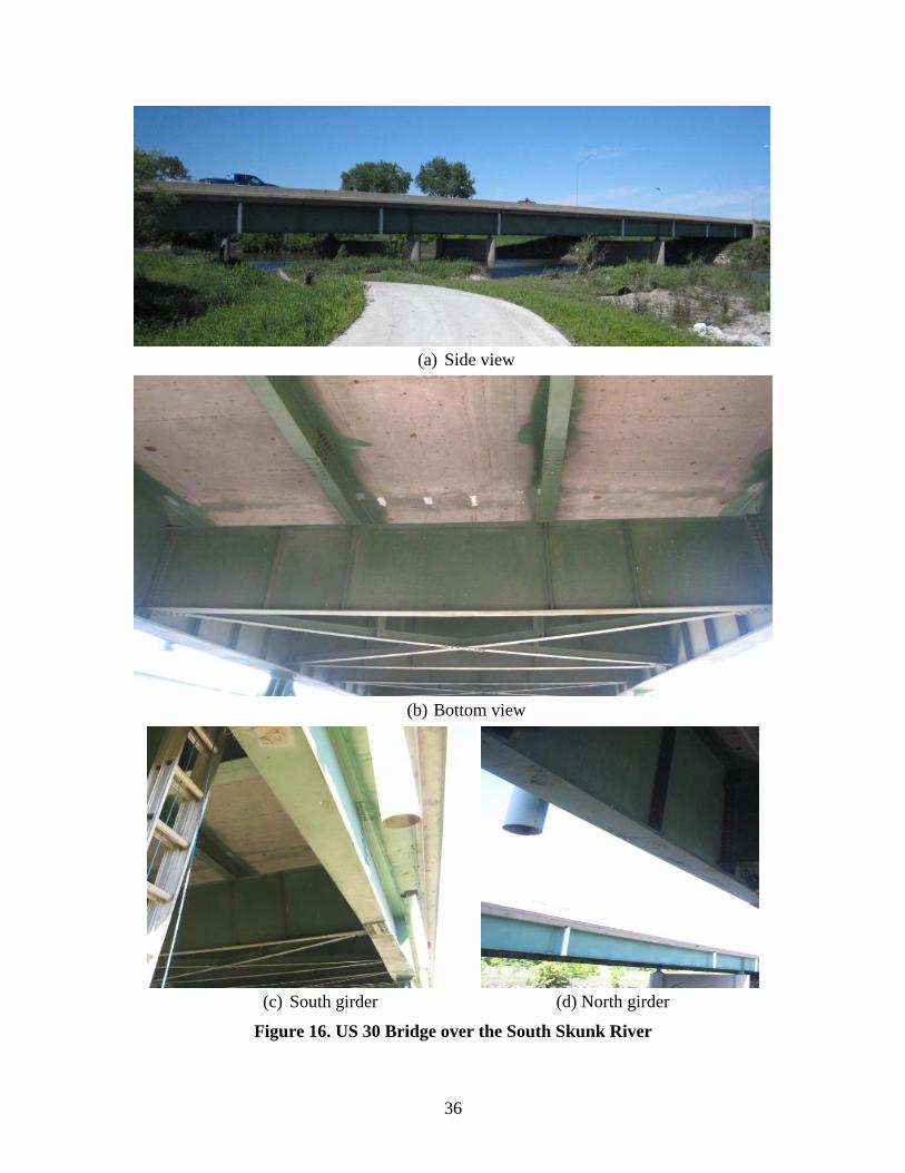
36
(a) Side view
(b) Bottom view
(c) South girder (d) North girder
Figure 16. US 30 Bridge over the South Skunk River

37
Figure 17. Wireless sensor node locations on US 30 Bridge
Figure 18. Weldable strain gauge
Node 649
Node 651
Node 639
Node 712
Base station

38
(a)
(b)
Figure 19. Solar panels (a) performance test (b) attached on the bridge (south side)

39
Figure 20. Wireless sensor node installed on the bridge

40
4.2 Strain Data Analysis
4.2.1 Overview of Data Preparation
Large amounts of data were available for analysis because wireless sensor nodes sample strains
at 128 Hz. As shown by previous research (Wipf et al. 2006), the useful information for the
evaluation procedures for a strain monitoring system is the quasi-static response of the bridge to
ambient traffic loads. Thus, the useful information needs to be extracted from the data.
The software Node Commander that came with SG-Link saves all data from a node into a
comma-separated values (CSV) file. The newly-received data are appended to the file. Each file
includes a file header for node information followed by time stamped data. The data in each row
are arranged according to the following format:
Time, Tick, Ch1, Ch3, Ch4, Node RSSI, Base RSSI
Time: Timestamp, which is the current coordinated universal time (UTC) in nanoseconds
Tick: Increment by 1 for each sweep within each session
Ch1, Ch3, Ch4: Measured data in Channel 1, 3, and 4, respectively
Node RSSI: Signal strength at which the node received the command from the base station
Base RSSI: Signal strength at which the base station received the response back from the
node
The file size increases quickly. Even with a duty cycle of 16.7 percent, the data file size of a
node with three active channels for 12 days is over 2 gigabytes. To prepare the data for further
processing, we need to separate the large file into smaller ones and extract the data collected for
the same period from all nodes. We developed a Python program to extract all four nodes’ strain
data for each session and generate one file for each.
Each session file includes data from all nodes for the same synchronized sample session. The file
size of each session is around 10 megabytes and thus is more manageable. The data preparation
and processing include removing the unwanted elements from the strain data to produce
consistent and useful information that can represent the quasi-static response of the bridge to
ambient traffic.
4.2.2 Segmental Analysis of Strain Records
The strain measurements are affected by many components, including mechanical strain
resulting from passing traffic and environmental factors. However, mechanical strains due to
traffic loadings occur much faster than those of temperature-induced strains, as pointed out by
Wipf et al. (2006). The records from wireless sensors also confirmed this behavior. The strain
records over 24 hours for four nodes are presented in Figure 21.

41
Figure 21. Strain plot of four sensor nodes over 24 hours
200
150
c 50 i" o; ~ c ·o;
ii -50
-150
-200
200
150
I 100
~ c ·~ 50 Ci1
0
v
-50 0
_j ~1---1 r f-- /
Strain over 24 hrs (Node 639)
10 Time (hour)
15 20
Strain over 24 hrs (Node 649)
I I I -~ t J -J AI Jl ~ .J. /1. J ..-1 1 vii\ • // ~ r r t'T v-t-
v 1-
10 15 20 Trme (hour)
Strain over 24 hrs (Node 71 2) 300,-----------------,-----------------,------------------,-----------------,-------------,
250
200
-50
"1000~----------------~----------------~10~--------------~15~--------------~2~0------------~
150
100
c 50 -~
-~ c o;
ii l'
-50
-100 0
--iV ~- ti-v v I
Time (hour)
Strain over 24 hrs (Node 651)
r-H+-~~i vv /[\ / r vf--V
10 15 20 Time (hour)

42
Note that the data are not continuous in burst mode. Data are collected for 5 minutes every 30
minutes and there are no data points between each 5 minute segment. In Figure 21, the slow
movement of the strain record is a result of the environmental temperature fluctuations, while the
short vertical spikes are strain resulting from passing traffic on the bridge.
The baseline movement due to temperature fluctuations may vary for different sensor nodes
because of the characteristic difference of individual sensing elements. Two enlarged 5 minute
data segments are presented in Figure 22 showing the strains within the short period (5 minutes
here). As shown, the baseline movement due to temperature fluctuation is a very slow change
over time compared to the strain resulting from ambient traffic; thus, the offset can be treated as
a constant.
4.2.3 Data Zeroing and Filtering
The strain change resulting from temperature fluctuation does not contain information related to
the quasi-static response of the bridge to the passing traffic. Therefore, the baseline strain offset
needs to be removed from the raw data. This process is called zeroing the data. The data
collected by the wireless sensor nodes are divided as 5 minute segments and the period is short
enough to consider the baseline as constant as discussed. Then, the DC offset can be removed. A
zero-phase filter is applied to remove the DC offset in MATLAB for each 5 minute segment.
The zeroed data may still contain noise in addition to the quasi-static strain response and
dynamic effects resulting from traffic loads. The frequency response can be obtained using the
MATLAB fast Fourier transform (fft) function. It can be seen that the frequencies of dynamic
effects are much higher than that of the quasi-static strain response, so a lowpass Chebyshev
filter is applied to remove the dynamic effects and high frequency noise (as discussed in Lu
2008). The parameters of the Chebyshev filter can be set as follows, as suggested by Lu (2008):
cutoff frequency 0.35 Hz and passband ripple 0.0873 decibels (dB).
In Figure 23, strain data of 5 minutes in the time domain (top figure) and its frequency response
(bottom figure) are plotted for Node 649. Node 649 was placed next to a wired fiber Bragg
grating (FBG) optical sensor that was installed for previous experiments. It can be seen that the
fundamental frequency of the bridge is 2.9 Hz while the quasi-static strain response is in the
frequencies lower than 1 Hz. Quasi-static strain contributed much more to the overall strain
signal power. The results are consistent with those of the wired FBG sensor (B-SG-BF-H) placed
in the same location (Wipf et al. 2006). This also validates the results for the wireless sensor
Node 649.
A MATLAB program was developed to process the data by applying a zero-phase filter and then
a Chebyshev filter. The program is able to process all the segment data files in a given directory
that have been created from the large master file. The zeroed and filtered data are then saved in
corresponding .CSV files. One example of the zeroed and filtered strain data is presented in
Figure 24.
43
(a) Strain records over the period of 6 days
(b) Strain record of the enlarged 24 hr period
(c) 5 minute Segment 1: 5:00 PM to 5:05 PM
(d) 5 minute Segment 2: 7:00 AM to 7:05 AM
Figure 22. Raw data baseline for small segment
Seg. 2
Seg. 1
24 hr

44
Figure 23. Frequency response
Figure 24. Zeroed and filtered strain data
The strain data were collected from Node 649 from 3:00 to 3:05 p.m. It can be seen from the data
that this was a busy traffic period with many vehicle events and multiple tracks passing. The top
(red) line across the bottom of the chart represents the processed signal, showing the mechanical
strain signal resulting from the ambient traffic on the bridge.
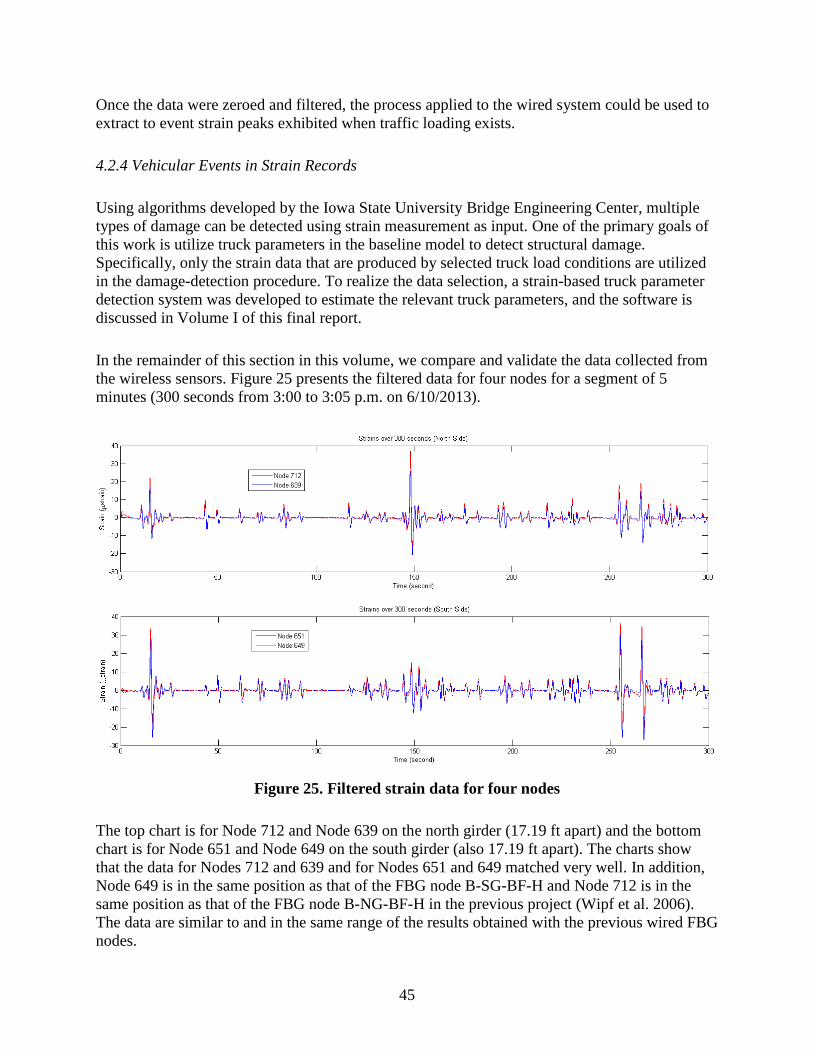
45
Once the data were zeroed and filtered, the process applied to the wired system could be used to
extract to event strain peaks exhibited when traffic loading exists.
4.2.4 Vehicular Events in Strain Records
Using algorithms developed by the Iowa State University Bridge Engineering Center, multiple
types of damage can be detected using strain measurement as input. One of the primary goals of
this work is utilize truck parameters in the baseline model to detect structural damage.
Specifically, only the strain data that are produced by selected truck load conditions are utilized
in the damage-detection procedure. To realize the data selection, a strain-based truck parameter
detection system was developed to estimate the relevant truck parameters, and the software is
discussed in Volume I of this final report.
In the remainder of this section in this volume, we compare and validate the data collected from
the wireless sensors. Figure 25 presents the filtered data for four nodes for a segment of 5
minutes (300 seconds from 3:00 to 3:05 p.m. on 6/10/2013).
Figure 25. Filtered strain data for four nodes
The top chart is for Node 712 and Node 639 on the north girder (17.19 ft apart) and the bottom
chart is for Node 651 and Node 649 on the south girder (also 17.19 ft apart). The charts show
that the data for Nodes 712 and 639 and for Nodes 651 and 649 matched very well. In addition,
Node 649 is in the same position as that of the FBG node B-SG-BF-H and Node 712 is in the
same position as that of the FBG node B-NG-BF-H in the previous project (Wipf et al. 2006).
The data are similar to and in the same range of the results obtained with the previous wired FBG
nodes.

46
Using the 17 µstrain as the threshold (Lu 2008), four truck events can be observed during the 5
minute period. The enlarged strain curves for Node 649 and Node 712 in three 30 second
segments are plotted in Figure 26.
Figure 26. Three 30 second segments of filtered strain data for Node 649 and Node 712
The data follows the typical strain pattern for girder bottom flange strain gauges for trucks.
Together with sensors in other locations, truck type and parameters may be determined. The peak
strain event can be further extracted using MATLAB functions. In Figure 27, both local positive
and negative peaks detected in duration of 30 seconds are shown in small triangles. Overall,
wireless sensors provide similar results as the wired strain gauge data acquisition system.

47
Figure 27. Positive and negative peaks
4.3 Energy Harvesting and Self-Sustainability Evaluation
Although potential energy resources are renewable for harvesting, they are still limited in
magnitude and each node must be as energy-efficient as possible to achieve self-sustainability.
The energy sources, including the solar panels used in this project, are typically irregular and
intermittent.
We wanted to evaluate if the wireless sensor nodes can achieve self-sustainability and operate
without or with minimal maintenance. For this purpose, super-capacitor voltage was monitored
during the two test periods. The capacitor voltages for the four wireless sensor nodes are
presented in Figure 28.
Notice the voltage shown is the voltage of one super-capacitor. According to the test results in
the lab, the capacitance is not exactly the same for the two super-capacitors in serial, but the
difference is small enough that we can assume the power supply voltage is twice of one super-
capacitor.

48
a) 12 day test
b) 6 day test
Figure 28. Sample capacitor voltage records
In the first test shown in Figure 28(a), Node 649 worked properly throughout the 12 days. Node
712 lost communication for 5 hours during the second day and was back to work properly. The
circuit in Node 639 stopped working during the fifth day and drew abnormally large current from
the super-capacitor. Node 651 communication worked properly but the energy harvester had
some issues, so it harvested significantly less energy than other nodes and the voltage dropped
below the cutoff voltage 1.45V every day after midnight.
Breaks in the waveform for Node 639 are when the super-capacitors did not have enough voltage
to power the node and therefore no samples were available. However, this demonstrated that
automatic recovery worked successfully. Once the supply voltage returned to 3V, the node

49
resumed synchronous sampling and transmission of data. It turned out the failures were due to
the soldering of surface-mounted ICs.
After replacing some ICs, the nodes were put back for the second test. The super-capacitor
voltage results for the second (6 day) test are presented in Figure 28(b). The initial super-
capacitor voltages were measured as follows:
Node 649: 2.38V Node 651: 1.68V
Node 712: 2.14V Node 639: 1.70V
As shown in the figure, the nodes were working properly except for Node 639. Node 639 worked
during the first 1.5 days and then lost its connection. After testing the EHSuperCap, it was found
to be working. Even though the super-capacitor voltage was still above 2V, this SG-Link node
stopped transmitting data back to the base station and needed reset.
Figure 28(b) shows the EHSuperCap board is able to provide enough energy to support the
operation of wireless sensors. Taking Node 651 as an example, it started at 1.68V and, after the
first day; it reached 2.23V at 7 p.m. The voltage kept dropping during the night and it reached its
low point at 7 a.m. at 1.87V before the voltage started to increase again for the daytime. The
lowest voltage it dropped to during the test was 1.85V, well above the required 1.5V. Overall, we
can see the nodes can be self-powered and maintain self-sustainability using a solar panel with a
270 cm2 area.
The available solar energy depends highly on the weather condition. The energy gain or loss
does not depend directly on temperature, but the temperature data give a general idea of daylight
time. The temperature data measured and weather conditions are presented for the 6 day test
duration in Figure 29.
Peak voltage follows daily temperature peaks in general, sometimes with a delay. Some of the
light intensity measurements are presented in Table 11.
The light level is between 800 and 2,000 FC around noon on the site measurement. The radiant
level changes quickly and significantly when clouds move in. The energy gained in the storage
(besides the energy that was consumed directly from the solar panel during the daytime) in Node
651 is presented in Figure 30.
The energy gain during the rainy, thunderstorm day (06/24/2013) is significantly less than other
days but still able to gain 270 J. Considering the energy loss during the nighttime, the overall
energy level decreased 130 J from the previous day. Assuming the super-capacitors are charged
initially to 2.4V, this allows operations on four continuous days under a similar
thunderstorm/rainy day before power is shutdown.

50
(a)
(b)
Figure 29. Temperature data versus voltage gain
Table 11. Light intensity level measured in the solar panel location
6/19/2013 6/20/2013 6/26/2013
South Side 1495FC at 11 a.m. 2065FC at 12 p.m. 2060FC at 1 p.m.
North Side 842FC at 11 a.m. 1160FC at 12 p.m. 1480FC at 1 p.m.
0
0.5
1
1.5
2
2.5
3
Cap
acit
or
Vo
ltag
e (
V)
Time
Node 651
clear clear overcast clear thunderstorm overcast clear thunderstorm rain partly cloudy mostly cloudy
Weather
Condition:
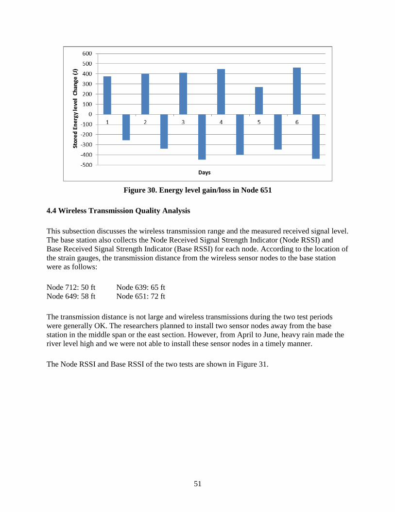
51
Figure 30. Energy level gain/loss in Node 651
4.4 Wireless Transmission Quality Analysis
This subsection discusses the wireless transmission range and the measured received signal level.
The base station also collects the Node Received Signal Strength Indicator (Node RSSI) and
Base Received Signal Strength Indicator (Base RSSI) for each node. According to the location of
the strain gauges, the transmission distance from the wireless sensor nodes to the base station
were as follows:
Node 712: 50 ft Node 639: 65 ft
Node 649: 58 ft Node 651: 72 ft
The transmission distance is not large and wireless transmissions during the two test periods
were generally OK. The researchers planned to install two sensor nodes away from the base
station in the middle span or the east section. However, from April to June, heavy rain made the
river level high and we were not able to install these sensor nodes in a timely manner.
The Node RSSI and Base RSSI of the two tests are shown in Figure 31.

52
(a) 6 day test
-80
-70
-60
-50
-40
-30
-20
-10
0
12
:30
6/2
0/2
01
3 1
8:3
0
6/2
1/2
01
3 0
:30
6/2
1/2
01
3 6
:30
6/2
1/2
01
3 1
2:3
0
6/2
1/2
01
3 1
8:3
0
6/2
2/2
01
3 0
:30
6/2
2/2
01
3 6
:30
6/2
2/2
01
3 1
2:3
0
6/2
2/2
01
3 1
8:3
0
6/2
3/2
01
3 0
:30
6/2
3/2
01
3 6
:30
6/2
3/2
01
3 1
2:3
0
6/2
3/2
01
3 1
8:3
0
6/2
4/2
01
3 0
:30
6/2
4/2
01
3 6
:30
6/2
4/2
01
3 1
2:3
0
6/2
4/2
01
3 1
8:3
0
6/2
5/2
01
3 0
:30
6/2
5/2
01
3 6
:30
6/2
5/2
01
3 1
2:3
0
6/2
5/2
01
3 1
8:3
0
6/2
6/2
01
3 0
:30
6/2
6/2
01
3 6
:30
6/2
6/2
01
3 1
2:3
0
No
de
RSS
I (d
Bm
)
Time
Node 712
Node 649
Node 639
Node 651
-90
-80
-70
-60
-50
-40
-30
-20
-10
0
12
:30
6/2
0/2
01
3 1
8:3
0
6/2
1/2
01
3 0
:30
6/2
1/2
01
3 6
:30
6/2
1/2
01
3 1
2:3
0
6/2
1/2
01
3 1
8:3
0
6/2
2/2
01
3 0
:30
6/2
2/2
01
3 6
:30
6/2
2/2
01
3 1
2:3
0
6/2
2/2
01
3 1
8:3
0
6/2
3/2
01
3 0
:30
6/2
3/2
01
3 6
:30
6/2
3/2
01
3 1
2:3
0
6/2
3/2
01
3 1
8:3
0
6/2
4/2
01
3 0
:30
6/2
4/2
01
3 6
:30
6/2
4/2
01
3 1
2:3
0
6/2
4/2
01
3 1
8:3
0
6/2
5/2
01
3 0
:30
6/2
5/2
01
3 6
:30
6/2
5/2
01
3 1
2:3
0
6/2
5/2
01
3 1
8:3
0
6/2
6/2
01
3 0
:30
6/2
6/2
01
3 6
:30
6/2
6/2
01
3 1
2:3
0
Bas
e R
SSI
(dB
m)
Time
Node 712
Node 649
Node 639
Node 651

53
(b) 12 day test
Figure 31. Node RSSI and Base RSSI
-90
-80
-70
-60
-50
-40
-30
-20
-10
0
17
:30
:00
6/7
/20
13
3:3
06
/7/2
01
3 1
3:3
06
/7/2
01
3 2
3:3
06
/8/2
01
3 9
:30
6/8
/20
13
19
:30
6/9
/20
13
5:3
06
/9/2
01
3 1
5:3
06
/10
/20
13
1:3
06
/10
/20
13
11
:30
6/1
0/2
01
3 2
1:3
06
/11
/20
13
7:3
06
/11
/20
13
17
:30
6/1
2/2
01
3 3
:30
6/1
2/2
01
3 1
3:3
06
/12
/20
13
23
:30
6/1
3/2
01
3 9
:30
6/1
3/2
01
3 1
9:3
06
/14
/20
13
5:3
06
/14
/20
13
15
:30
6/1
5/2
01
3 1
:30
6/1
5/2
01
3 1
1:3
06
/15
/20
13
21
:30
6/1
6/2
01
3 7
:30
6/1
6/2
01
3 1
7:3
06
/17
/20
13
3:3
06
/17
/20
13
13
:30
6/1
7/2
01
3 2
3:3
06
/18
/20
13
9:3
0
No
de
RSS
I (d
Bm
)
Time
Node 712
Node 649
Node 639
Node 651
-90
-80
-70
-60
-50
-40
-30
-20
-10
0
17
:30
:00
6/7
/20
13
4:3
0
6/7
/20
13
15
:30
6/8
/20
13
2:3
0
6/8
/20
13
13
:30
6/9
/20
13
0:3
0
6/9
/20
13
11
:30
6/9
/20
13
22
:30
6/1
0/2
01
3 9
:30
6/1
0/2
01
3 2
0:3
0
6/1
1/2
01
3 7
:30
6/1
1/2
01
3 1
8:3
0
6/1
2/2
01
3 5
:30
6/1
2/2
01
3 1
6:3
0
6/1
3/2
01
3 3
:30
6/1
3/2
01
3 1
4:3
0
6/1
4/2
01
3 1
:30
6/1
4/2
01
3 1
2:3
0
6/1
4/2
01
3 2
3:3
0
6/1
5/2
01
3 1
0:3
0
6/1
5/2
01
3 2
1:3
0
6/1
6/2
01
3 8
:30
6/1
6/2
01
3 1
9:3
0
6/1
7/2
01
3 6
:30
6/1
7/2
01
3 1
7:3
0
6/1
8/2
01
3 4
:30
6/1
8/2
01
3 1
6:3
0
Bas
e R
SSI
(dB
m)
Time
Node 712
Node 649
Node 639
Node 651

54
The charts show that the received signal levels in the base station and wireless sensor nodes are
symmetrical in general. Note that in Node 639, the SG-Link node failure caused discontinuance
of the transmission. The wireless measurement signal was between -55 decibel milliwatts (dBm)
and -80 dBm, while most wireless transceivers today have a receiver sensitivity of -80 dBm or
better. One of the common IEEE 802.15.4-compliant transceivers, Chipcon CC2530 from Texas
Instruments, has a receiver sensitivity of -97dBm. Chipcon transceivers are also used in SG-Link
nodes. The difference between the received signal level and receiver sensitivity is considered the
fading margin. With at least 15 dB in the fading margin in this case, the received signal level is
OK.
The design transmission range of SG-Link nodes for open areas is up to 2,000 meters (6,562 ft),
so we expect the nodes are able to meet the transmission requirements for most bridges.
However, because of the concrete and steel structure of bridges, the communication channel is
very different from open areas making the transmission distance shorter.
If there is a direct steel obstacle in the middle of the transmission path, the RF signal will be
attenuated significantly. The RF signal may also be received through multiple transmission paths
due to the bridge structure between the base station and sensor nodes. In the multiple path
propagation, pulses for the same signal will arrive at different times, and the received signal
strength may be attenuated or increased depending on the phase. Therefore, a short transmission
range does not necessarily provide a better RF transmission signal.
We can observe this in the Figure 31(a). Node 651 is the farthest away from the base station with
a transmission distance of 72 ft; however, both Node RSSI and Base RSSI are the best among the
four, while Node 712, with the minimum transmission range of 50 ft among the four, has the
worst Node RSSI for most of the time. One of the reasons is that, although Node 712 is closer to
the base station, the way it was placed (as shown Figure 20) makes the girder wall block the RF
signal between the node and the base station.

55
5. SUMMARY AND CONCLUSIONS
This volume discussed the activities related to objective 3 of this project: to evaluate the
hardware and energy harvesting techniques for a self-powered bridge monitoring wireless sensor
network. As wireless communication gains popularity, applying wireless sensor networks to
bridge monitoring becomes a natural alternative because a significant cost of any bridge
monitoring system lies in the cost of cabling and its installation.
Most wireless sensors are powered using batteries and can last a limited time, especially for high
sample frequency demanding applications. With this project, a minimum 125 Hz sample rate was
needed. With a sample rate of 128 Hz, three high-capacity D-cell batteries (assuming 1.5V,
18,000 mA each) can provide only a two-month power supply to SG-Link nodes. It is not
convenient or cost-efficient to replace batteries. Therefore, a self-powered wireless sensor
network is a very attractive option. A self-sustainable wireless sensor node can support its
operation by harvesting energy from the environment and, thus, its lifetime is limited only by the
lifetime of the electronics.
The hardware of the system demonstrated includes four wireless sensor nodes and a base station
that serves as the data aggregator. Each wireless sensor node consists of a traditional metallic foil
strain gauge, an energy harvesting and power management circuit, a film solar panel, and a
wireless senor platform that provides raw data collection and communication with the base
station.
Ambient energy sources were first compared based on the energy density and availability.
Although a great deal of research work is on the energy harvesting from bridge vibration caused
by passing traffic, the collectable energy level is very low and not cost-efficient at this stage.
Solar energy is still the best choice due to its high energy density, high conversion efficiency,
and mature technology with solar cells.
After reviewing the current energy harvesting techniques and energy storage components for
wireless sensors, an energy harvesting circuit (EHSuperCap) with two super-capacitors as the
energy storage was developed. The system prototype was tested on the demonstration bridge.
Two field tests of the system consisting of four wireless sensor nodes were conducted, lasting 12
days and 6 days, respectively. Strain measurement, super-capacitor voltage, and temperature
information were collected. The received data at the base station were saved as a CSV file that
was updated when new data were received.
A basic data process, including zeroing and filtering, was performed. The test results were
analyzed to validate the wireless sensor data collected. The results demonstrated that using a 270
cm2 solar panel next to a sensor node, the system can maintain the energy balance to collect
strain data with a 16.7 percent duty cycle in a sample frequency of 128 Hz.

56
The transmission signal quality and energy harvesting results were also analyzed and discussed.
The communication was reliable overall, but a few failures did occur during the tests. The node
is shut down when the power supply voltage falls below 3V and is able to return to the
synchronous sampling state automatically when the accumulated energy is enough to cold start
the node.
The wireless sensor node installation was quick and convenient. The protection enclosure is
lightweight and small and can be fixed on the bridge using heavy-duty Velcro tape. Along with
the weldable strain gauges and bendable film solar panel, installation is simple.
One complete wireless sensor node costs a little over $700 to date, including $545 for the
wireless sensor platform, $22.45 for two super-capacitors, $31.49 for a film solar panel, $72.97
for a strain gauge, and about $45 for the energy harvesting and power management circuit board.
The major cost is the wireless sensor platform. The unit cost can be lowered if the volume is
large. Each base station costs $700 to $1,000, depending on which model is used. Overall, a
wireless bridge system using strain gauges may cost $3,000 or more for the hardware, depending
on the number of nodes needed. For a system with 14 nodes, the hardware costs would be around
$10,500.
A wireless sensor network for bridge monitoring is promising but also has limitations.
Conclusions and recommendations for further research are as follows:
The demonstrated wireless bridge monitoring system using wireless sensor nodes is suitable
for implementation. The nodes are very easy to install and the cost of a system is reasonable.
Because of its easy installation and redeployment, the system is especially attractive when
the bridge monitoring system needs to be deployed in multiple bridges and the number of
sensor nodes for each site is not very large, or for short-term structure monitoring and testing.
After completing tests at one site, the nodes can be simply removed and moved to another
site for another short-term monitoring period, such as several days or a couple of weeks.
The communication throughput could be an issue for a large network with low-cost wireless
sensor nodes for application with high sample rate requirements. The most common
communication standard used in wireless sensor networks is IEEE 802.15.4, which provides
only the raw data rate of 250 kilobytes per second (kbps). Considering the communication
overhead and retransmission, the actual payload data rate could be less than 10 kBps. If
multiple nodes are connected to the base station for data uploading or synchronous
transmission, the bandwidth for each node is reduced. The node may not be able to transmit
data back on time and synchronous burst mode should be used to prevent data loss.
When a node works in synchronous burst mode, it collects a given number of samples for a
given interval. The collected data is not continuous but still provides the strain information
resulting from ambient traffic. Given the strain data give more usable information during
traffic-dense periods, such as rush hours, the nodes may be set to take more samples during

57
the traffic-dense hours and save energy during other periods. One issue that needs addressed
is how to better utilize the information obtained during burst mode sampling and its impact
on the performance of the SHM system.
Another area that can be exploited is bridge monitoring applications that do not demand high
sample frequency, such as crack or water level monitoring.
Overall, energy harvesting-based wireless sensor networks are an attractive option for
various bridge monitoring applications.


59
REFERENCES
Aktakka, E. E., Peterson, R. L., Najafi, K. (2011). A self-supplied inertial piezoelectric energy
harvester with power-management IC, Solid-State Circuits Conference Digest of
Technical Papers (ISSCC), 2011 IEEE International. pp. 120, 121, Feb. 20-24 2011.
Alippi, C., and Galperti, C. (2008). “An Adaptive System for Optimal Solar Energy Harvesting
in Wireless Sensor Network Nodes.” IEEE Transactions on Circuits and Systems I:
Regular Papers. vol.55, no.6, pp. 1742-1750, July 2008.
Anton, Steven R. (2011). Multifunctional Piezoelectric Energy Harvesting Concepts, PhD
dissertation, Virginia Polytechnic Institute and State University, 2011.
Arms, S. W., Townsend, C. P., Galbreath, J. H., and Newhard, A. T. (2004). Wireless strain
sensing networks, in Proceedings of the European Workshop on Structural Health
Monitoring, July 2004.
Banks, B., Harms, T., Sedigh Sarvestani, S., Bastianini, F. (2009). A low-cost wireless system
for autonomous generation of road safety alerts, Proceedings of the SPIE, Vol. 7292, 8
pp.
Becker, T., Kluge, M., Schalk, J., Otterpohl, T., and Hilleringmann, U. (2008). “Power
management for thermal energy harvesting in aircrafts.” IEEE Sensors, pp. 681, 684, Oct.
26-29, 2008.
Beeby, S. P., Tudor, M., and White, N. (2006). “Energy Harvesting Vibration Sources for
Microsystem Applications.” Measurement Science and Technology, Vol. 17, No.12, pp.
R175-R195.
Bouchouicha, D., Latrach, M., Dupont, F., and Ventura, L. (2010). An experimental evaluation
of surrounding RF energy harvesting devices, Microwave Conference (EuMC), 2010
European. pp. 1381, 1384. Sept. 28-30, 2010.
Brunelli, D., Benini, L., Moser, C., and Thiele, L. (2008). An Efficient Solar Energy Harvester
for Wireless Sensor Nodes, Design, Automation and Test in Europe, 2008. DATE '08.
vol., no., pp. 104, 109, March 10-14, 2008.
Brunelli, D., Moser, C., Thiele, L., and Benini, L. (2009). “Design of a Solar-Harvesting Circuit
for Batteryless Embedded Systems.” IEEE Transactions on Circuits and Systems I:
Regular Papers. vol. 56, no. 11, pp. 2519, 2528, Nov. 2009.
Cadex Electronics. Supercapacitor. Accessed July 11, 2013. Available at:
batteryuniversity.com/learn/article/whats_the_role_of_the_supercapacitor.
Chen, Z., Guerrero, J. M., and Blaabjerg, F. (2009). “A review of the state of the art of power
electronics for wind turbines.” IEEE Trans. Power Electron. vol. 24, no. 8, pp.1859 -
1875, 2009.
Chintalapudi, K., Fu, T., Paek, T., Kothari, N., Rangwala, S., Caffrey, J., Govindan, R., Johnson,
E., and Masri, S. (2006). “Monitoring Civil Structures with a Wireless Sensor Network.”
Internet Computing. IEEE. vol. 10, no. 2, pp. 26-34, March-April 2006.
Dalola, S., Ferrari, V., Guizzetti, M., Marioli, D., Sardini, E., Serpelloni, M., and Taroni, A.
(2008). Autonomous Sensor System with RF Link and Thermoelectric Generator for
Power Harvesting, Instrumentation and Measurement Technology Conference
Proceedings, 2008. IMTC 2008. IEEE, pp.1376, 1380, May 12-15, 2008.
DeWolf, John T. (2009). History of Connecticut’s Short-Term Strain Program for Evaluation of
Steel Bridges. Connecticut Department of Transportation. Bureau of Engineering and
Construction. July 2009

60
Dondi, D., Bertacchini, A., Brunelli, D., Larcher, L., and Benini, L. (2008). “Modeling and
Optimization of a Solar Energy Harvester System for Self-Powered Wireless Sensor
Networks.” IEEE Transactions on Industrial Electronics. Vol.55, No. 7, pp. 2759, 2766.
July 2008.
Fairchild Semiconductor. FSA1156/FSA 1157 data sheet. Last accessed October 3, 2013.
Available at fairchildsemi.com/pf/FS/FSA1156.html.
FHWA Bridge Programs NBI Data: Bridges by Posting Status. (2012). Accessed July 15, 2013.
Available at www.fhwa.dot.gov/bridge/nbi/no10/posting12.cfm.
Galchev, T., McCullagh, J., Peterson, R. L., and Najafi, K. (2011). Harvesting traffic-induced
bridge vibrations, In Proceedings of 2011 IEEE 16th International Solid-State Sensors,
Actuators and Microsystems Conference (TRANSDUCERS), pp. 1661, 1664, June 5-9,
2011.
Gorlatova, M., Sharma, T., Shrestha, D., Xu, E., Jiasi Chen, Skolnik, A., Dongzhen Piao, Kinget,
P., Kymissis, J., Rubenstein, D., and Zussman, G. (2010). Prototyping Energy Harvesting
Active Networked Tags (EnHANTs). with MICA2 Motes, Sensor Mesh and Ad Hoc
Communications and Networks (SECON), 2010 7th Annual IEEE Communications
Society Conference. pp. 1, 3, 21-25. June 2010.
Green, M. A., Emery, K., Hishikawa, Y., Warta, W. and Dunlop, E. D. (2013). “Solar cell
efficiency tables (version 42).” Progress in Photovoltaics: Research and Applications,
Vol. 21. No.5. pp. 827-837. August 2013.
IEEE Standard 802.15.4: Wireless Medium Access Control (MAC). and Physical Layer (PHY).
Specifications for Low-Rate Wireless Personal Area Networks (LR-WPANs).
Jo, Hongki, Sung-Han Sim, Kirill A. Mechitov, Robin Kim, Jian Li, Parya Moinzadeh, Billie F.
Spencer, Jr., Jong Woong Park, Soojin Cho, Hyung-Jo Jung, Chung-Bang Yun, Jennifer
A. Rice, and Tomonori Nagayama. (2011). Hybrid Wireless Smart Sensor Network for
Full-Scale Structural Health Monitoring of a Cable-Stayed Bridge. The SPIE Conference,
San Diego, CA, March 6-10, 2011.
Joshi, Harshvardan P., Burlacu, Bogdan, Prabhu, Manjunath M., Yoon, Suyoung, Sichitiu,
Mihail L., Dutta, Rudra, Rizkalla, and Sami H. (2006). Wireless Structural Health
Monitoring System Design, Implementation and Validation. Center for Advanced
Computing and Communications (CACC), Raleigh, NC, January 2006.
Kim, Junhee, R. Andrew Swartz, Jerome P. Lynch, Jong-Jae Lee, and Chang-Geun Lee. (2010).
“Rapid-to-Deploy Reconfigurable Wireless Structural Monitoring Systems using
Extended-Range Wireless Sensors.” Smart Structures and System. TechnoPress.
6(5-6):505-524.
Kim, Sehwan, No, Keun-Sik, and Chou, P. H. (2011). “Design and Performance Analysis of
Supercapacitor Charging Circuits for Wireless Sensor Nodes.” Emerging and Selected
Topics in Circuits and Systems, IEEE Journal. Vol. 1, No.3, pp. 391, 402. Sept. 2011.
Kim, Robin E., Nagayama, T., Jo, H., and Spencer Jr., B. F. (2012). Preliminary study of low-
cost GPS receivers for time synchronization of wireless sensor networks. 2012 SPIE,
Smart Structures and Nondestructive Evaluation and Health Monitoring, San Diego, CA.
Li, Jian, Nagayama, Tomonori, Mechitov, Kirill A., and Spencer Jr., Billie F. (2012). Efficient
campaign-type structural health monitoring using wireless smart sensors, Proc. SPIE
8345, Sensors and Smart Structures Technologies for Civil, Mechanical, and Aerospace
Systems 2012, 83450U, April 26, 2012.

61
Li, Mo, and Liu, Yunhao. (2007). Underground structure monitoring with wireless sensor
networks, Proceedings of ACM 6th International Symposium on Information Processing
in Sensor Networks, p. 69(10), April 25-27, 2007.
Linear Technology. LTC2915/LTC2916 Data sheet. Last accessed Oct. 3, 2013. Available at
cds.linear.com/docs/en/datasheet/29156fa.pdf.
LORD MicroStrain Sensing Systems. SG-Link-LXRS Wireless Strain Node. Accessed July 10,
2013. Available at: microstrain.com/wireless/sg-link.
Lu, Ping. (2008). A Statistical Based Damage Detection Approach for Highway Bridge
Structural Health Monitoring. PhD dissertation. 2008.
Lynch, Jerome P., and Loh, Kenneth (2006). “A Summary Review of Wireless Sensors and
Sensor Networks for Structural Health Monitoring.” Shock and Vibration Digest, Sage
Publications, 38(2):91-128, March 2006.
Mascarenas, D., Flynn, E., Farrar, C., Park, G., and Todd, M. (2009). “A Mobile Host Approach
for Wireless Powering and Interrogation of Structural Health Monitoring Sensor
Networks.” Sensors Journal, IEEE. vol.9, no.12, pp.1719, 1726, Dec. 2009.
Mateu, Loreto, and Moll, Francesc. (2005). Review of energy harvesting techniques and
applications for microelectronics, Proceedings of the SPIE, Vol. 5837, pp. 359-373, 2005.
Maxwell Technologies. Design Considerations for Ultracapacitors. Accessed June 10, 2012.
Available at:
maxwell.com/products/ultracapacitors/docs/200904_whitepaper_designinguide.pdf.
Mechitov, Kirill, W. Kim, and G. Agha. (2006). “High-Frequency Distributed Sensing for
Structure Monitoring.” Trans. of the Society of Instrument and Control Engineers (SICE),
vol. E-S-1, no. 1, 2006.
MTI MicroFuel Cells Inc. The Mobion Chip Breakthrough. MTI Micro product information.
Accessed July 15, 2013. Available at:
mtimicrofuelcells.com/technology/breakthrough.asp.
Musiani, D., Lin, K., and Rosing, T. S. (2007). Active sensing platform for wireless structural
health monitoring, Proceedings of ACM 6th International Symposium on Information
Processing in Sensor Networks, p. 390(10), April 25-27, 2007.
Nordblom, T., and Galbreath, J. (2012) Wireless Sensor Networks for Improved Long-Term
Bridge Performance, Microstrain white paper, 2012.
Oozeki, T., Yamada, T., Otani, K., Takashima, T. and Kato, K. (2010), “Performance trends in
grid-connected photovoltaic systems for public and industrial use in Japan.” Progress in
Photovoltaics. 18:596–602. Dec. 2010.
Paek, Jeongyeup, Chintalapudi, K., Govindan, R., Caffrey, J., and Masri, S. (2005). A Wireless
Sensor Network for Structural Health Monitoring: Performance and Experience,
Proceedings of 2nd IEEE Workshop on Embedded Networked Sensors, p1(10), May 30-
31, 2005.
Pakzad, Shamim N., Fenves, Gregory L., Kim, Sukun, and Culler, David E. (2008). “Design and
Implementation of Scalable Wireless Sensor Network for Structural Monitoring.” ASCE
Journal of Infrastructure Engineering, Vol. 14, Issue 1, pp. 89-101. March 2008.
Paradiso, J. A., and Starner, T. (2005). “Energy Scavenging for Mobile and Wireless
Electronics.” IEEE Pervasive Computing, 4:1, pp.18-27, Jan.-March 2005.

62
Park, Chulsung, and Chou, Pai. H. (2006). AmbiMax: Autonomous Energy Harvesting Platform
for Multi-Supply Wireless Sensor Nodes, SECON '06. 3rd Annual IEEE
Communications Society on Sensor and Ad Hoc Communications and Networks, vol.1,
pp. 168-177, Sept. 28, 2006.
Park, Gyuhae, Rosing, Tajana, Todd, Michael D., Farrar, Charles R., and Hodgkiss, William.
(2008). “Energy Harvesting for Structural Health Monitoring Sensor Networks.” ASCE
Journal of Infrastructure Systems, SPECIAL ISSUE: New Sensors, Instrumentation, and
Signal Interpretation, Vol. 14(1), pp. 64-79, 2008.
Raghunathan, V., Kansal, A., Hsu, J., Friedman, J., and Srivastava, M. B. (2005). Design
considerations for solar energy harvesting wireless embedded systems, Fourth
International Symposium on Information Processing in Sensor Networks. pp. 457-462,
April 15, 2005.
Raju, Murugavel, and Grazier, Mark. (2010). Energy Harvesting: ULP meets energy harvesting:
A game-changing combination for design engineers, Texas Instruments White Paper.
April 2010.
Rice, J. A., and Spencer Jr., B. F. (2008). Structural health monitoring sensor development for
the Imote2 platform, Proc. SPIE Smart Structures/NDE, 2008.
Roundy, Shad, Steingart, Dan, Frechette, Luc, Wright, Paul, and Rabaey, Jan. (2004). “Power
Sources for Wireless Sensor Networks.” Lecture Notes in Computer Science. Vol. 2920,
pp. 1-17, 2004.
Rowe, D. M. (2006). Chapter 1.3 Thermoelectric Generation and the Figure-of-Merit. In
Thermoelectrics Handbook: Macro to Nano. CRC Press, 2006.
Salim, M. D., and Zhu, J. (2010). Wireless Sensor Networks for Infrastructure Monitoring.
University of Northern Iowa, Cedar Falls, Iowa, October 2010.
Sazonov, Edward, R. Jha, K. Janoyan, V. Krishnamurthy, M. Fuchs, and K. Cross. (2006).
Wireless Intelligent Sensor and Actuator Network (WISAN): a scalable ultra-low-power
platform for structural health monitoring. Proceedings of SPIE’s Annual International
Symposium on Smart Structures and Materials, San Diego, CA, 2006.
Sazonov, E., Haodong Li, Curry, D., and Pillay, P. (2009). “Self-Powered Sensors for
Monitoring of Highway Bridges.” IEEE Sensors Journal, vol. 9, no. 11, pp. 1422, 1429,
Nov. 2009.
Schaevitz, Samuel B. (2012). Powering the wireless world with MEMS, Micromachining and
Microfabrication Process Technology XVII. Proceedings of the SPIE, Vol. 8248, pp. 15.
Shen, Hui, J. Qiu, H. Ji, K. Zhu, M. Balsi, I. Giorgio, and F. Dell’Isoloa. (2010). “A low-power
circuit for piezoelectric vibration control by synchronized switching on voltage sources.”
Sensors and Actuators A: Physical, No.5, 245-255, May 6, 2010.
Simjee, F., and Chou, P. H. (2006). Everlast: Long-life, Supercapacitor-operated Wireless Sensor
Node,. Proceedings of the 2006 International Symposium on Low Power Electronics and
Design. ISLPED '06., pp.197-202, Oct 4-6, 2006.
Sodano, Henry A., Inman, Daniel J., and Park, Gyuhae. (2005). “Comparison of Piezoelectric
Energy Harvesting Devices for Recharging Batteries.” Journal of Intelligent Material
Systems and Structures. 16(10), 799-807, Oct. 2005.
Strasser, M., R. Aigner, C. Lauterbach, T. F. Sturm, M. Franosch, G. Wachutka. (2003).
“Micromachined CMOS thermoelectric generators as on-chip power supply,” Sensors
and Actuators A, 114, 362-370. Jan. 2003

63
Tabesh, Ahmadreza, and Fréchette, Luc G. (2008). Ultra low power stand-alone circuitry for
harvesting energy from a micro-power piezoelectric generator, Proceedings of
PowerMEMS + microEMS 2008, Sendai, Japan, 2008, pp. 289-292, Nov. 9-12.
Tan, Yen Kheng, and Panda, S. K. (2011). “Optimized Wind Energy Harvesting System Using
Resistance Emulator and Active Rectifier for Wireless Sensor Nodes.” IEEE
Transactions on Power Electronics, vol.26, no.1, pp.38, 50, Jan. 2011.
Taneja, J., J. Jeong, and D. Culler. (2008). Design, Modeling, and Capacity Planning for Micro-
Solar Power Sensor Networks. International Conference on Information Processing in
Sensor Networks, IPSN '08. pp. 407-418, April 22-24, 2008.
Torah. R. N., M. J. Tudor, K. Patel, I. N. Garcia, and S. P. Beeby. (2007). Autonomous low
power microsystem powered by vibration energy harvesting, Proceedings of 6th Annual
IEEE Conference on Sensors, Atlanta, Georgia, pp. 264-267, Oct. 28-31, 2007.
U.S. Energy Information Administration. Electric Power Monthly with Data for May 2013, July
2013. Accessed August 10, 2013. Available at: eia.gov/electricity/monthly/pdf/epm.pdf.
Vishay Precision Group. Special Use Strain Gages - Weldable Strain Gages. Micro-
Measurements. Accessed July 15, 2013. Available at:
vishaypg.com/docs/11533/sealweld.pdf.
Wang, Y., Lynch, J. P., and Law, K. H. (2007). “A wireless structural health monitoring system
with multithreaded sensing devices: Design and validation,” Structure and Infrastructure
Engineering - Maintenance, Management and Life-Cycle Design & Performance. 3(2),
103-120. 2007.
Weddell, A. S., Merrett, Geoff V., Kazmierski, T. J., and Al-Hashimi, B. M. (2011), “Accurate
Supercapacitor Modeling for Energy Harvesting Wireless Sensor Nodes.” IEEE
Transactions on Circuits and Systems II: Express Briefs, vol. 58, no. 12, pp. 911, 915,
Dec. 2011.
Weimer, M. A., Paing, T. S., and Zane, R. A. (2006). Remote area wind energy harvesting for
low-power autonomous sensors, Proc. 37th IEEE Power Electron. Spec. Conf., pp.2911 -
2915, 2006.
Wipf, T. J., B. M. Phares, L. F. Greimann, D. Hemphill, J. D. Doornink, and P. Lu. (2006).
Remote Continuous Evaluation of a Bridge Constructed Using High-Performance Steel.
Bridge Engineering Center, Iowa State University, Ames, Iowa. May 2006.
Wipf, T. J., B. M. Phares, L. F. Greimann, D. Wood, and J. D. Doornink. (2007). Evaluation of
Steel Bridges Phase II. Bridge Engineering Center, Iowa State University, Ames, Iowa.
December 2007.
Wu, Guangxi, and Yu, Xiong. (2012). “System design to harvest thermal energy across
pavement structure,” Energytech, 2012 IEEE. pp. 1, 4. May 29-31, 2012.
Wu, Jingxian, and Zhou, Guoqing. (2011). A New Ultra-Low Power Wireless Sensor Network
with Integrated Energy Harvesting, Data Sensing, and Wireless Communication. IEEE
International Conference on Communications (ICC). vol., no., pp.1, 5. June 5-9, 2011.