The Japanese Geotechnical Society

Soils and Foundations

Soils and Foundations 2014;54(2):197–208

http://d0038-0

nCorE-mPeer

x.doi.org/806 & 201

respondinail addrereview un

www.sciencedirect.comjournal homepage: www.elsevier.com/locate/sandf

Integration of construction control and pile setup into loadand resistance factor design of piles

Kam Nga,n, Sri Sritharanb

aDepartment of Civil and Architectural Engineering, University of Wyoming, USAbDepartment of Civil, Construction and Environmental Engineering, Iowa State University, USA

Received 21 May 2013; received in revised form 13 September 2013; accepted 14 November 2013Available online 14 April 2014

Abstract

Regionally developed Load and Resistance Factor Design (LRFD) recommendations for bridge pile designs are enhanced by integrating theconstruction control capability of dynamic analysis methods and the recently developed pile setup quantification method in the calibrationprocess. Using a high quality, electronic Pile LOad Test (PILOT) database and 10 recently completed full-scale pile tests, resistance factors weredeveloped using a reliability theory for a locally calibrated static analysis method and two dynamic analysis methods: the Wave EquationAnalysis Program (WEAP) and the CAse Pile Wave Analysis Program (CAPWAP). Pile design efficiency was improved by minimizing thediscrepancy between design and field pile resistances through a proposed probability-based construction control method. The efficiency of bridgefoundations was further increased by incorporating the economic advantages of pile setup into the LRFD recommendations. Compared withrecommendations made by Paikowsky et al. (2004), Canadian Engineering Society (2006) and American Association of State Highway andTransportation Officials (2003), regionally-calibrated resistance factors were improved.& 2014 The Japanese Geotechnical Society. Production and hosting by Elsevier B.V. All rights reserved.

Keywords: WEAP; PDA; CAPWAP; Resistance factors; Construction control; Pile setup; LRFD; IGC: E4

1. Introduction

In an effort to ensure uniform reliability of bridge founda-tions in the United States, Load and Resistance Factor Design(LRFD) philosophy has been progressively developed sincethe early 1990s. The limit state design equation adopted by the

10.1016/j.sandf.2014.02.0104 The Japanese Geotechnical Society. Production and hosting by

g author.ss: kng1@uwyo.edu (K. Ng).der responsibility of The Japanese Geotechnical Society.

American Association of State Highway and TransportationOfficials (2012) is expressed as

∑γiQirφR ð1Þ

where Qi is the applied load, R is the nominal pile resistance, γiis the load factor corresponding to load Qi, and φ is thegeotechnical resistance factor. Uncertainties associated withresistance (R) are principally related to site characterization,soil variability, design method, and construction practice.According to Paikowsky et al. (2004), these uncertainties aresignificantly different from those that affect the applied load(Q). To account for the difference in uncertainties, the appliedload (Q) and resistance (R) are multiplied separately by thesuitable load factor (γ) and resistance factor (φ), respectively,

Elsevier B.V. All rights reserved.

K. Ng, S. Sritharan / Soils and Foundations 54 (2014) 197–208198

thereby targeting more consistent and reliable performance ofbridge foundations.

Recognizing the advantages of LRFD philosophy, theFederal Highway Administration (FHWA) mandated that allnew bridges initiated after October 1, 2007 should follow theLRFD approach. However, because the current AASHTO(2012) LRFD Bridge Design Specifications do not reflect localsoil conditions, design methods, and construction practices,resulting foundation designs may be overly conservative andunnecessarily costly. For economic reasons and to avoidunnecessarily conservative pile designs, regionally calibratedLRFD resistance factors have been permitted by the AASHTO.In response to this provision in the AASHTO, extensive soilinvestigations and 10 full-scale field tests on steel H-piles wereconducted by Ng et al. (2011a) to populate the historical PileLOad Tests (PILOT) electronic database compiled by Rolinget al. (2011). The test data are publically available at theproject website (http://srg.cce.iastate.edu/lrfd/). The researchfocused on the steel H-pile, because it is the most commonfoundation type used for bridges in the United States(AbdelSalam et al., 2010a). Using the PILOT database andrecently completed pile test results, regionally-calibratedLRFD resistance factors were determined for (1) a LocallyCalibrated Design Method (LCDM), and (2) two constructioncontrol methods, Wave Equation Analysis Program (WEAP)and CAse Pile Wave Analysis Program (CAPWAP) forverifying the pile performance during construction. TheLCDM method utilizes a design chart of unit resistancesdeveloped by Dirks and Kam (1989), which is summarizedin Green et al. (2012). This method is based on a combinationof the α-method by Tomlinson (1971) for cohesive materialsand the Meyerhof (1976) semi-empirical method for cohesion-less materials given by

qs ¼ αSu; qt ¼ NncSu ðTomlinson; 1971Þ

qs ¼N 0 ; qt ¼ 40N0bDbb r400N

0b ðMeyerhof; 1976Þ ð2Þ

where qs and qt are the unit side friction and unit end bearing,respectively, α is the adhesion factor, Su is the undrained shearstrength in soil adjacent to the pile, Nn

c is the bearing capacityfactor, N

0is the average corrected SPT blow counts along the

pile, Db is the pile embedment depth in the bearing stratum,and b is the pile diameter/width. In other words, the resistanceof a pile embedded in a mixed soil is estimated using theα-method for cohesive soil and the semi-empirical method forcohesionless soil. WEAP is a one-dimensional analysis ofhammer–pile–soil model, which simulates the pile motion andthe force generated by the hammer to drive the pile andestablishes a pile driving bearing graph (Rausche et al., 1985).CAPWAP matches PDA measured pile force and velocity withthat estimated using a one-dimensional pile–soil model (PileDynamics Inc., 2000).

Attaining pile resistance assumed in design during construc-tion presents challenges, because piles are designed usingstatic analysis methods, and the actual pile resistanceis verified during construction by means of a constructioncontrol method. These challenges will increase costs, delay

construction schedules, and create contractual challenges.Therefore, a probabilistic approach by integrating the con-struction control capability of WEAP and CAPWAP into thepile design stage using LCDM is proposed.The efficiency of bridge foundations can be further improved

by incorporating pile setup into pile designs. Pile setup refers tothe increase in resistance of a driven pile as a function of timestarting from the End of Driving (EOD) of the pile. Pile setupoccurs due to healing of remolded soils, increase in lateralstresses of surrounding soil on the pile, and dissipation of porewater pressure (Ng et al., 2013a). However, routinely recom-mended design methods (e.g.; the Canadian EngineeringSociety, 2006; the AASHTO, 2012) do not include setup inthe LRFD specifications for two reasons:

(1)

Lack of experimental data validating the accuracy ofexisting empirical methods for estimating pile setup; and

(2)

Calibration procedure to incorporate the pile setup compo-nent into the LRFD framework was not available untilrecently using the pile setup quantification method devel-oped and verified by Ng et al. (2012) and the calibrationprocedure proposed by Ng et al. (2011b). The effects ofpile setup can now be considered and incorporated into theLRFD of piles.

2. Development of resistance factors

2.1. Pile LOad Test (PILOT) database

To improve the pile foundation design practices, the IowaDepartment of Transportation (DOT) in the United Statesconducted 264 static pile load tests between 1966 and 1989.These historical test records were compiled into an electronicPILOT database for efficient data analysis. Of the 264 testsentered into PILOT, 164 were performed on steel H-piles.Eighty of these steel H-piles had the pile and soil informationrequired for static analysis using LCDM: 34 in sand, 20 in clayand 26 in mixed soil. Thirty-two of the 80 records assummarized in Table 1 had the information required forconstruction control analysis using WEAP. The PILOT data-base contains no pile strain and acceleration measurements,typically recorded using a Pile Driving Analyzer (PDA), whichare required in subsequent CAPWAP analysis. Table 1 showsthe measured pile resistances (Rm) obtained from static loadtests (SLTs) based on the Davisson's criterion (Davisson,1972), estimated pile resistances (RE) using LCDM, andestimated pile resistances at the EOD (REOD) using WEAP.To identify uncertainties resulting from different soil

behaviors, the data were sorted as either sand, clay, or mixedsoil profile, using a 70%-rule established by AbdelSalam et al.(2011) in the development of LRFD resistance factors for staticanalysis methods. Accordingly, a site is identified as a sand orclay profile site if the soil along the pile embedded length ismore than 70% of the respective soil type when classified inaccordance to the Unified Soil Classification System (USCS).

Table 1Summary of 32 pile records from PILOT database that have sufficient information for WEAP analyses.

Soil profile ID Iowa County Pile size Hammer Time ofSLT (Day)

Rm (kN) Re (kN) Hammer blowcount (bl/300 mm)

REOD (kN)

Sand 10 Ida HP 250� 63 Gravity 2 516 592 5 28417 Fremont HP 250� 63 Gravity 5 587 632 13 97320 Muscatine HP 250� 63 Kobe K-13 5 534 721 40 77024 Harrison HP 250� 63 Gravity 9 818 770 23 110834 Dubuque HP 250� 63 Delmag D-12 7 996 899 37 68848 Black Hawk HP 250� 63 Gravity 5 641 734 10 57870 Mills HP 250� 63 Delmag D-12 5 569 850 30 62274 Benton HP 250� 63 Kobe k-13 32 667 1001 34 61799 Wright HP 250� 63 Gravity 7 463 654 7 411151 Pottawattamie HP 250� 63 Delmag D-22 4 890 681 11 604158 Dubuque HP 360� 132 Kobe K-42 4 2589 2006 60 2961

Clay 6 Decatur HP 250� 63 Gravity 3 525 556 8 31412 Linn HP 250� 63 Kobe K-13 5 907 756 46 68942 Linn HP 250� 63 Kobe K-13 5 365 391 19 37844 Linn HP 250� 63 Delmag D-22 5 605 672 24 41851 Johnson HP 250� 63 Kobe K-13 3 845 850 36 57057 Hamilton HP 250� 63 Gravity 4 747 681 11 41662 Kossuth HP 250� 63 MKT DE-30B 5 445 654 21 33663 Jasper HP 250� 63 Gravity 2 294 423 13 26364 Jasper HP 250� 63 Gravity 1 543 534 15 31567 Audubon HP 250� 63 Delmag D-12 4 623 627 24 536102 Poweshiek HP 250� 63 Gravity 8 578 569 13 375109 Poweshiek HP 310� 79 Delmag D-12 3 783 854 48 653

Mixed 7 Cherokee HP 250� 63 Gravity 6 783 694 11 4718 Linn HP 250� 63 Kobe K-13 8 756 654 34 640

25 Harrison HP 250� 63 Delmag D-12 4 996 503 36 64543 Linn HP 250� 63 Delmag D-22 5 632 872 22 74246 Iowa HP 250� 63 Gravity 4 730 796 11 58466 Black Hawk HP 250� 63 Mit M14S 5 801 618 32 53573 Johnson HP 250� 63 Kobe K-13 6 1032 792 30 57290 Black Hawk HP 310� 79 Gravity 4 845 947 26 868106 Pottawattamie HP 250� 63 Gravity 6 658 498 7 334

Rm¼measured pile resistance determined from static load test based on the Davisson's criterion; SLT¼static load test; Re¼estimated pile resistance using theLCDM; and REOD¼estimated pile resistance at the end of driving using WEAP.

K. Ng, S. Sritharan / Soils and Foundations 54 (2014) 197–208 199

If a site contains less than 70% sand and 70% clay, then it isidentified as a mixed soil site.

2.2. Field test data

To collect pile strain and acceleration records for CAPWAPanalysis and pile setup data as well as to populate the existingPILOT database, 10 full-scale pile tests were conducted in thestate of Iowa, USA. These pile tests involved detailed sitecharacterization using both in-situ subsurface investigationsand laboratory soil tests. Prior to pile driving, the HP250 testpiles, denoted as ISU1 through ISU10 as summarized inTable 2, were instrumented with strain gauges along theembedded pile length. In accordance with the 70%-rule, testpiles ISU9 and ISU10 were embedded in sand profiles, testpiles ISU2 to ISU6 were embedded in clay profiles, and testpiles ISU1, ISU7, and ISU8 were embedded in mixed soilprofiles. PDA measurements and pile driving resistances interms of hammer blow counts were recorded first during piledriving, then at EOD and finally during several restrikes. Pile

restrikes were performed on all test piles except ISU1 todetermine the change in pile resistances as a function of timeelapsed since the EOD. After the last restrike, a vertical SLTwas performed on each test pile following the “Quick Test”procedure in accordance with the American Society for Testingand Materials (ASTM) D1143 (2007). Table 2 shows the pilerecords and their respective measured pile resistances (Rm)obtained from SLTs based on the Davisson's criterion(Davisson, 1972), estimated pile resistances (Re) using LCDM,and estimated pile resistances at EOD (REOD) and at thebeginning of restrike (RBOR) using WEAP and CAPWAP. Thefield test results showed that pile setup in clay and mixed soils,but not in sand (Ng et al., 2011a). Since the developedmethodology only accounts for pile setup in clay (Ng et al.,2013b), pile setup in mixed soil is neglected in this paper.

2.3. Calibration method

First Order Second Moment (FOSM) suggested by Barkeret al. (1991) was used to calibrate the resistance factor. Despite

Table 2Summary of 10 pile records from field tests at EOD and last restrike.

Test pileID

Soilprofile

IowaCounty

Pile size Hammer Time ofSLT (day)

Rm

(kN)Time of lastrestrike(day)

Re

(kN)WEAP CAPWAP

REOD

(kN)RBOR

(kN)REOD

(kN)RBOR

(kN)

ISU1 Mixed Mahaska HP 250� 85 Delmag D19-42 100 881 N/A 565 473 N/A 631 N/AISU2 Clay Mills HP 250� 63 Delmag D19-42 9 556 2.97 191 343 614 359 578ISU3 Clay Polk HP 250� 63 Delmag D19-32 36 667 1.95 378 366 585 440 658ISU4 Clay Jasper HP 250� 63 Delmag D19-42 16 685 4.75 467 422 688 453 685ISU5 Clay Clarke HP 250� 63 Delmag D16-32 9 1081 7.92 391 635 1138 790 1088ISU6 Clay Buchanan HP 250� 63 Delmag D19-42 14 946 9.81 480 624 1122 644 937ISU7 Mixed Buchanan HP 250� 63 Delmag D19-42 13 236 9.76 151 41 292 51 331ISU8 Mixed Poweshiek HP 250� 63 Delmag D19-42 15 721 4.95 578 607 811 621 710ISU9 Sand Des Moines HP 250� 63 APE D19-42 25 703 9.77 792 737 667 751 688ISU10 Sand Cedar HP 250� 63 APE D19-42 6 565 4.64 743 685 593 538 526

Rm¼measured pile resistance determined from static load test based on Davisson's criterion; SLT¼static load test; Re¼estimated pile resistance using the LCDM;REOD¼estimated pile resistance at the end of driving; RBOR¼pile resistance determined at the beginning of last restrike; and N/A¼not available.

K. Ng, S. Sritharan / Soils and Foundations 54 (2014) 197–208200

its simplicity, FOSM provides results that are comparable toother more rigorous reliability methods (Bloomquist et al.,2007). Paikowsky et al. (2004) compared FOSM to therigorous and invariant First Order Reliability Method (FORM)and found a difference in the outcomes of approximately 10%,with the FOSM method leading to smaller resistance factors.By contrast, the Monte-Carlo method produced resistancefactors about 10% to 20% higher than those found with theFOSM method (Allen, 2005).

The FOSM method requires both the total load (Q) and totalresistance (R) to be lognormally distributed and mutuallyindependent. Focusing on axial pile resistance, the AASHTO(2012) Strength I load combination (i.e., dead and live loadsonly) was considered in this study. Nowak (1999) observedthat the lognormal distribution better characterizes the loadsand suggested the numerical values for the different probabil-istic characteristics of dead (QD) and live (QL) loads (γ, λ, andCOV), as recapitulated in parentheses in Eq. (3). To verify thatpile resistance follows a lognormal distribution, a hypothesistest based on the Anderson and Darling (1952) normalitymethod was used to assess the Goodness of Fit of the assumeddistributions. The AD method was preferred because of itsappropriateness for small sample size (Romeu, 2010). Theresistance factor (φ) was determined using Eq. (3); derivationof this equation can be found in the Reference Manual andWorkbook published by National Highway Institute (2001).

φ¼λR

γDQDQL

þγL

� � ffiffiffiffiffiffiffiffiffiffiffiffiffiffiffiffiffiffiffiffiffiffiffiffiffiffiffiffiffiffiffiffiffiffið1þCOV2

D þCOV2LÞ

ð1þCOV2RÞ

h ir

λDQDQL

þλL� �

e βTffiffiffiffiffiffiffiffiffiffiffiffiffiffiffiffiffiffiffiffiffiffiffiffiffiffiffiffiffiffiffiffiffiffiffiffiffiffiffiffiffiffiffiffiffiffiffiffiffiffiffiln ½ð1þCOV2

RÞð1þCOV2DþCOV2

LÞ�p� � ð3Þ

where λR is the resistance bias factor of the resistance ratio,COVR is the coefficient of variation of the resistance ratio, γD,γL is the dead load factor (1.25) and live load factor (1.75), λD,λL is the dead load bias (1.05) and live load bias (1.15), COVD,COVL are coefficients of variation of dead load (0.1) and liveload (0.2), βT is the target reliability index, and QD/QL is thedead to live load ratio.

The LRFD resistance factors calibration requires selection ofa set of target reliability levels represented by target reliabilityindices (βT), which describe the probability of failures (Pf).According to Barker et al. (1991), the target reliability indexfor driven piles can be reduced to a value between 2.0 and 2.5,especially to account for a group effect. The initial targetreliability indices used by Paikowsky et al. (2004) werebetween 2 and 2.5 for pile groups, and as high as 3.0 for asingle pile. Paikowsky et al. (2004) recommended targetreliability indices of 2.33 (corresponding to 1% probabilityof failure) and 3.00 (corresponding to 0.1% probability offailure) for representing redundant and non-redundant pilegroups, respectively. To maintain consistency with the recom-mendations suggested by Paikowsky et al. (2004) and adoptedby the AASHTO (2012), these recommended βT values wereselected in this study.Dead to live load ratios (QD/QL) of 0.52, 1.06, 1.58, 2.12,

2.64, 3.00,and 3.53 were suggested in AASHTO for bridgespan lengths of 9, 18, 27, 36, 45, 50, and 60 m (30, 59, 89,148, 164, and 197 ft), respectively. Paikowsky et al. (2004)used a QD/QL ratio ranging from 2.0 to 2.5, while Allen (2005)used a conservative ratio of 3.0. Due to the frequent use ofshort span bridges in Iowa, the DOT used a QD/QL ratio of 1.5.To strike a balance between two extremes (0.52 for 9 m and3.53 for 60 m bridge spans), an average QD/QL ratio of 2.0 wasselected in this study. However, it is worth nothing asconcluded by Paikowsky et al. (2004) that resistance factorsare insensitive to the choice of a QD/QL ratio.The foregoing FOSM method is appropriately used for

calculating a resistance factor for pile resistance (R) defined asa single random variable, i.e., pile resistance is determinedfrom a single procedure or method. However, the incorpora-tion of pile setup in the LRFD requires a new calibrationprocedure that can separately and simultaneously account forthe different uncertainties associated with the initial pileresistance at EOD (REOD) and pile setup resistance (Rsetup)while achieving the same target reliability level. A detailedstudy conducted by Ng et al. (2011b) confirmed that different

Table 3Summary of adjusted measured pile resistances at EOD and setup resistancesfor clay profile.

Pile ID Measured pileresistance at EOD,Rm-EOD (kN)

Measured pile setupresistance, Rm-setup

(kN)

Estimated pile setupresistance, Re-setup

(kN)

WEAP CAPWAP WEAP CAPWAP WEAP CAPWAP

ISU2 316 320 240 236 270 285ISU3 359 402 308 266 281 285ISU4 396 452 289 233 310 213ISU5 649 754 432 327 378 344ISU6 561 668 385 278 457 2146 343 N/A 182 N/A 139 N/A12 602 N/A 306 N/A 438 N/A42 238 N/A 126 N/A 341 N/A44 395 N/A 210 N/A 244 N/A51 579 N/A 266 N/A 253 N/A57 472 N/A 275 N/A 186 N/A62 298 N/A 147 N/A 205 N/A63 190 N/A 104 N/A 217 N/A64 366 N/A 177 N/A 102 N/A67 408 N/A 214 N/A 410 N/A

K. Ng, S. Sritharan / Soils and Foundations 54 (2014) 197–208 201

uncertainties arise from the use of different procedures inestimating the two resistance components, and the correspond-ing two resistances (i.e., REOD and Rsetup) were determined tobe statistically independent. Hence, the REOD is determined byeither WEAP or CAPWAP while Rsetup is estimated usingEq. (4) proposed by Ng et al. (2011a).

Rt

REOD¼ Clog10

t

tEOD

� �þ1

; Rsetup ¼ Rt�REOD ð4Þ

where Rt is the pile resistance at time (t) after EOD, Na is theweighted average uncorrected SPT N-value, tEOD is the time atEOD assumed as 1 min, and C is the pile setup rate described interms of Na as shown in Fig. 1 and their relationship is given by

C¼ a

ðNaÞbð5Þ

where a is an empirical coefficient (0.215 and 0.432 for REOD

determined by WEAP and CAPWAP, respectively), and b is anempirical coefficient (0.144 and 0.606 for REOD determined byWEAP and CAPWAP, respectively). The reliability of this pilesetup method was evaluated as follows:

102 365 N/A 213 N/A 230 N/A109 516 N/A 267 N/A 477 N/A

(1)

Pile

Set

up R

ate

(C)

Fig.SPT

N/A¼not available.

Add the estimated pile setup resistance (Re-setup) given inTable 3 to the estimated REOD given in Table 1 for piledata in clay from PILOT;

(2)

Also add the estimated pile setup resistance (Re-setup) givenin Table 3 to the estimated REOD given in Table 2 for thefull-scale test piles in clay; and

(3)

Compare the total estimate pile resistance (REODþRsetup)determined from above with the measured pile resistance(Rm) obtained from SLT.

Following this evaluation procedure, Ng et al. (2011a)concluded that the anticipated errors of the pile setup methodat the 90% confidence level were determined to be between�13.9% and �0.5% for WEAP and �4.9% and 3.8% forCAPWAP.

To account for the different uncertainties associated with theresistance components, the LRFD limit state Eq. (1) was

C = 0.432 Na-0.606

C = 0.215 Na-0.144

0.06

0.08

0.1

0.12

0.14

0.16

0.18

0.2

0 2 4 6 8 10 12 14 16 18Weighted Average SPT N-Value, Na

CAPWAPWEAPISU2

ISU2ISU3

ISU3

ISU4

ISU4

ISU5

ISU5

ISU6

ISU6

1. The relationship between the rate of pile setup and weighted averageN-value

expanded to Eq. (6) by multiplying different resistance factorsφEOD and φsetup to REOD and Rsetup, respectively.

∑γiQirφEODREODþφsetupRsetup ð6ÞThe φEOD value was determined using Eq. (3) while the φsetup

value was determined using Eq. (7) developed by Ng et al.(2011b). The same probabilistic characteristics (γ, λ, COV) ofthe loads recommended by Nowak (1999) (i.e., the QD/QL

ratio of 2.0 and both βT values of 2.33 and 3.00) were chosen.The calculated probabilistic characteristics (λ, COV) and theφEOD value were input in Eq. (7) to determine the φsetup value.

φsetup ¼λsetup

γDQDQL

� �þ γL

1þ QDQL

� � �φEOD

24

35

λDQDQL

� �þ λL

1þ QDQL

� �0@

1Ae

βT

ffiffiffiffiffiffiffiffiffiffiffiffiffiffiffiffiffiffiffiffiffiffiffiffiffiffiffiffiffiffiffiffiffiffiffiffiffiffiffiffiffiffiffiffiffiffiffiffiffiffiffiffiffiffiffiffiffiffiffiffiffiffiffiln ½ð1þCOV2

REODþCOV2

RsetupÞð1þCOV2

QDþCOV2

QL�

p

ffiffiffiffiffiffiffiffiffiffiffiffiffiffiffiffiffiffiffiffiffiffiffiffiffiffiffiffiffiffiffiffiffið1þ COV2

QDþ COV2

QLÞ

ð1þCOV2REOD

þCOV2Rsetup

Þ

r �λEOD

ð7Þ

2.4. Resistance factors for sand and mixed soil profiles

Figs. 2–4 show the lognormally distributed cumulativedensity function (CDF) plots of resistance ratios (RRs) forLCDM, WEAP and CAPWAP, respectively. The resistanceratio (RR) is generally defined as a ratio of measured nominalpile resistance to estimated nominal pile resistance. To imple-ment Eq. (1), the statistical parameters of RR given by Eqs. (8)and (9) were used as input in Eq. (3) to determine theresistance factor (φ). The mean and standard deviation of a

101

99

90

50

10

1

101

99

90

50

10

1

Sand

Ratio of Measured to Estimated (Nominal Resistance)

Perc

ent o

f Mea

sure

d ≤

Est

imat

ed R

esis

tanc

e Clay

Mixed

Loc 0.07810Scale 0.3843N 36AD 0.367

Sand

Loc 0.2923Scale 0.3938N 25AD 0.275

Clay

Loc 0.1262Scale 0.3646N 29AD 0.299

Mixed

Fig. 2. Cumulative density functions for the Locally Calibrated Design Method (LCDM)

10.01.00.1

10.01.00.1

99

90

50

10

1

10.01.00.1

99

90

50

10

1

Sand

Ratio of Measured to Estimated (Nominal Resistance)

Perc

ent o

f Mea

sure

d ≤

Est

imat

ed R

esis

tanc

e

Clay-EOD Clay-Setup

Clay-BOR Mixed

Loc 0.001138Scale 0.3189N 13AD 0.175

Sand

Loc -0.08871Scale 0.1625N 17AD 0.295

Clay-EOD

Loc -0.1619Scale 0.4118N 17AD 0.183

Clay-Setup

Loc -0.03910Scale 0.1138N 5AD 0.189

Clay-BOR

Loc 0.3724Scale 0.3083N 11AD 0.144

Mixed

Fig. 3. Cumulative density functions for WEAP

K. Ng, S. Sritharan / Soils and Foundations 54 (2014) 197–208202

lognormal distribution of each RR are given as “Loc” and“Scale”, respectively, in the CDF plots. The normallydistributed resistance bias (λR) and coefficient of variation(COVR) were back-calculated using Eqs. (8) and (9), respec-tively.

λR ¼ e½Locþ0:5 lnð1þCOV2RÞ� ð8Þ

COVR ¼ffiffiffiffiffiffiffiffiffiffiffiffiffiffiffiffiffiffiffiffiffiffiðeScale2 �1Þ

qð9Þ

The RR is a ratio of SLT measured pile resistance at time (t)to estimated pile resistance determined by LCDM or at theEOD condition determined by either WEAP or CAPWAP (seeTables 1 and 2). No pile setup was considered in this analysis.Using the probabilistic characteristics of RR (λR and COVR)based on both PILOT and field tests, the regional resistancefactors (φ) for sand and mixed soil were calculated andpresented in Table 4. However, the resistance factors alonecannot be used to measure the efficiency of various methods,because the efficiency of each method is highly influenced by

99

90

50

10

1

2.01.00.5

2.01.00.5

99

90

50

10

1

2.01.00.5

99

90

50

10

1

All Soils-EOD

Ratio of Measured and Estimated (Nominal Resistance)

Perc

ent o

f Mea

sure

d ≤

Est

imat

ed R

esis

tanc

eAll Soils-BOR Sand

Clay-EOD Clay-Setup Clay-BOR

Mixed

Loc 0.02720Scale 0.1410N 9AD 0.462

All Soils-EOD

Loc 0.007901Scale 0.1614N 10AD 1.173

All Soils-BOR

Loc -0.008862Scale 0.08098N 2AD 0.250

Sand

Loc -0.04403Scale 0.06286N 5AD 0.177

Clay-EOD

Loc 0.008493Scale 0.1724N 5AD 0.231

Clay-Setup

Loc -0.004436Scale 0.02060N 5AD 0.374

Clay-BOR

Loc 0.2413Scale 0.1308N 2AD 0.250

Mixed

Fig. 4. Cumulative density functions for CAPWAP

K. Ng, S. Sritharan / Soils and Foundations 54 (2014) 197–208 203

the respective λR (Paikowsky et al., 2004). To normalize theinfluence of λ on φ, the efficiency of different methods wasevaluated using an efficiency factor (φ/λ), which defines as aratio of resistance factor to its respective resistance bias.A higher φ/λ value correlates to a better efficient pile designmethod. Table 4 shows that the regionally-calibrated φ valuesfor LCDM in sand and mixed soil are higher than thoserecommended by Paikowsky et al. (2004), while the regionalφ/λ values are slightly lower. Similarly, the regionally-calibrated φ values for LCDM are higher than those recom-mended in AASHTO (2012) and CES (2006).

The regionally calibrated φ and φ/λ values for WEAP andCAPWAP at the EOD condition are higher than thoserecommended in the aforementioned three references. Com-pared with the results for WEAP, Table 4 shows thatCAPWAP provides better pile resistance estimations withrespect to the measured pile resistances, indicated by λR valuescloser to one and smaller COVR values. However, it isimportant to note that the resistance factors determined forCAPWAP shall be used with caution due to the relativelysmall sample sizes used in this study. Instead, resistancefactors of CAPWAP for the “All Soil” profile given inTable 4 should be used. Overall, the regional database hasimproved the calibrated results for piles in sand and mixed soilprofiles.

2.5. Resistance factors for clay profile

The calibration of resistance factors for the clay profile,based on both PILOT and field test data, was performeddifferently from the sand and mixed soil, because pile setup

was considered in the clay profile. The RRs for clay profile aredescribed as follows:

(1)

For design stage, RR is a ratio of SLT measured pileresistance (Rm) to estimated pile resistance (Re) determinedusing LCDM.

(2)

For construction stage, RR for EOD is a ratio of SLTmeasured pile resistance adjusted from time (t) to the EOD(Rm-EOD) (see Table 3) to estimated pile resistance determinedat the EOD (REOD) using either WEAP or CAPWAP(Tables 1 and 2). Since no static load tests were performedat EOD, Rm-EOD was back-calculated using Eq. (4) byreplacing the Rt with the SLT measured resistance (Rm) atthe corresponding time (t) when SLT was performed.

(3)

For construction stage, RR for BOR is a ratio of SLTmeasured pile resistance (Rm) to estimated pile resistancedetermined at the beginning of last restrike test (RBOR) usingeither WEAP or CAPWAP (see Table 2). This is applicableto pile construction projects, where a pile performance isverified using restrikes (i.e., ΣγiQirφBOR RBOR).

(4)

For construction stage, RR for setup is a ratio of measuredpile setup resistance (Rm-setup) and estimated pile setupresistance (Re-setup) given in Table 3. The Rm-setup value isthe difference between SLT measured pile resistance (Rm)and the previously described Rm-EOD. The Re-setup valuewas determined using Eq. (4) at time (t) when each SLTwas performed and based on calculated Na value as well asthe constant empirical coefficients a and b.

To be implemented in Eq. (6), the statistical parameters (λRand COVR) of RR were used in both Eqs. (3) and (7) todetermine φEOD and φsetup, respectively. The effect of pile

Table 4Regionally-calibrated results and their comparisons.

Stage Method Data source Soil profile Condition N λR COVR β¼2.33 β¼3.00

φ φ/λ φ φ/λ

Design LCDM Iowa Sand General 36 1.16 0.37 0.55 0.47 0.41 0.36Clay 25 1.44 0.41 0.63 0.43 0.46 0.32Mixed 29 1.20 0.34 0.60 0.50 0.46 0.38

Meyerhof Paikowskyet al. (2004)

Sand 18 0.81 0.38 0.42 0.51 0.32 0.39α-method Clay 17 0.82 0.40 0.40 0.49 0.31 0.37α-method; Nordlund Mixed 20 0.59 0.39 0.30 0.51 0.23 0.39Meyerhof AASHTO (2012) Sand – – – 0.30 – 0.24 –

α-method Clay and Mixed – – – 0.35 – 0.28 –

Static analysis method CES (2006) All soil – – – 0.40 – 0.40 –

Construction WEAP Iowa Sand EOD 13 1.05 0.33 0.54 0.52 0.42 0.40Clay EOD 17 0.93 0.16 0.65 0.70 0.54 0.58

BORa 5 0.97 0.11 0.72 0.75 0.61 0.63Setup 17 0.93 0.43 0.26 0.28 0.20 0.21

Mixed EOD 11 1.52 0.31 0.80 0.53 0.62 0.41Paikowsky et al. (2004) All soil EOD 99 1.66 0.72 0.39 0.24 0.25 0.15AASHTO (2012) All soil EOD or BOR – – – 0.50 – 0.40 –

CES (2006) All soil EOD – – – 0.40 – 0.40 –

CAPWAP Iowa All soil EOD 9 1.04 0.14 0.75 0.72 0.63 0.60All soil BORb 10 1.02c 0.16c 0.71 0.70 0.59 0.58Sanda EOD 2 0.99 0.08 0.77 0.77 0.66 0.66Claya EOD 5 0.96 0.06 0.75 0.78 0.64 0.67

Setup 5 1.00 0.17 0.59 0.58 0.49 0.49BOR 5 0.99 0.02 0.80 0.80 0.69 0.69

Mixeda EOD 2 1.28 0.13 0.94 0.73 0.79 0.62Paikowsky et al. (2004) All Soil EOD 125 1.63 0.49 0.64 0.39 0.46 0.28

EOD(ARo350 andBlow counto16 bl/10 cm)

37 2.59 0.92 0.41 0.16 0.23 0.09

BOR 162 1.16 0.34 0.65 0.56 0.51 0.44AASHTO (2012) All Soil BORd

– – – 0.80 – 0.64 –

BORe– – – 0.75 – 0.60 –

BORb– – – 0.65 – 0.52 –

CES (2006) All soil EOD – – – 0.50 – 0.50 –

CES¼Canadian Engineering Society.aThe resistance factors shall be used with caution due to the relatively small sample size available for this study.bDynamic tests on at least two piles per site condition, but no less than 2% of the production piles.cCannot satisfy the lognormal distribution.dAt least one static load test and two dynamic tests per site condition, but no less than 2% of the production piles.eDynamic tests on 100% production piles.

K.Ng,

S.Sritharan

/Soils

andFoundations

54(2014)

197–208

204

K. Ng, S. Sritharan / Soils and Foundations 54 (2014) 197–208 205

setup in clay profiles is incorporated into the LRFD bycomputing the φsetup values using the proposed setup Eq.(4). Due to a higher uncertainty involved in estimating the pilesetup resistance (COVR¼0.43), a smaller φsetup value of 0.29for WEAP based on βT¼2.33 was determined using Eq. (7).However, a larger φsetup value of 0.59 for CAPWAP wasdetermined as the uncertainty represented by a smaller COVR

of 0.17 decreased.The application of these resistance factors follows the

revised LRFD limit state Eq. (6), which can be rewritten as

∑γiQirφEODREODþφsetupREOD

alog10t

tEOD

� �ðNaÞb

24

35 ð10Þ

Rearranging this equation, REOD becomes the target nominalpile driving resistance at EOD (Rtarget-EOD), which needs to beverified using either WEAP or CAPWAP during construction.

Rtarget�EODZ∑γiQi

φEODþφsetup

alog10t

tEOD

� �ðNaÞb

24

35

ð11Þ

Note that the entire denominator of Eq. (11) is always higherthan the resistance factor of LCDM and α-method given inTable 4, because the φEOD of 0.65 for WEAP or 0.75 forCAPWAP alone given in Table 4 at βT¼2.33 is larger than theφ values of 0.63 for LCDM and 0.35 or 0.40 for α-method.The Rtarget-EOD determined by Eq. (11) with due considerationto pile setup will be smaller than that without considering setup(i.e., no φsetup term and φEOD¼general φ) due to a largerdenominator for the same ΣγQ. The integration of pile setupinto the LRFD will (1) shorten pile embedment length, becausea smaller target pile resistance will be achieved duringconstruction; (2) reduce the chance of re-tapping of piles afterEOD, for which the assumed target pile driving resistance atEOD based on static analysis method has not been met; and (3)provide the economic advantages of pile setup while comply-ing with the LRFD framework and ensuring a targetreliability level.

Table 4 shows that the regionally calibrated resistance factors forthe clay profile are generally greater than those recommended by

Table 5Construction control and resistance factors for the LCDM.

Constructioncontrol method

Soil profile Construction control factor (ξ)

EOD Setup BOR Total Limit S

WEAP Clay 0.75 1.16 – 0.87 1.32 1Mixed 1.07 – – 1.07 1.90 1Sand 0.94 – – 0.94 1.34 1

CAPWAP Clay 0.87 1.25 – 1.08 1.37 1– – 1.38 1.38 1.27 1

Mixed – – 1.18 1.18 1.63 1Sand – – 1.06 1.06 1.25 1

aThe minimum value of 1.00 was suggested (i.e., construction control considerabThis value was suggested so that the modified φ for the LCDM does not exce

Paikowsky et al. (2004), AASHTO (2012) and CES (2006).The anticipated economic benefit of this approach based on arecent study using 604 production piles is that the incorporation ofpile setup in clay reduces the target driving resistance (Rtarget-EOD)by about 17% (Ng et al., 2012). The application of the proposedapproach was demonstrated by Green et al. (2012).

3. Construction control

3.1. Introduction

To minimize the difference in pile resistances estimatedduring design stage using the LCDM and during constructionusing WEAP or CAPWAP, a probability-based constructioncontrol analysis was performed to integrate WEAP andCAPWAP as part of the design procedure. Data from bothPILOT and recently completed field tests were selected forWEAP, while only the field tests were used for the CAPWAPevaluation due to the availability of PDA data. The WEAP andCAPWAP analyses were performed for three resistance condi-tions in total: EOD, setup, and BOR as summarized in Table 5.

3.2. Methodology

Construction control is integrated into design by multiplyinga construction control factor (ξ) for the respective resistancecondition to the originally calibrated resistance factor (φ).Adopting the suggestion given by Paikowsky et al. (2004) forother influential factors, such as site variability, quality of soilparameters, construction control quality and site/constructionexperience, the LRFD limit state equation for considering theconstruction control factor is expressed as

∑γiQirΠξiφR ð12ÞThe product of construction control factors (Πξi) can be expressedspecifically for various resistance conditions as follows:

1.

ugg

.00a

.07

.00a

.08

.27b

.18

.06

tioned 0

EOD condition only: Πξi¼ξEOD,

2. EOD condition plus setup (in clay): Πξi¼ξEOD� ξsetup, and 3. BOR condition: Πξi¼ξBOR,

Resistance factor (φ) of the LCDM for β¼2.33 % Gain in φ

est Original Modified

0.63 0.63 00.60 0.64 70.55 0.55 0

0.63 0.68 80.63 0.80 270.60 0.71 180.55 0.58 6

is not considered)..80.

K. Ng, S. Sritharan / Soils and Foundations 54 (2014) 197–208206

product of all applicable construction control factors, φ is

where γi is the load factor, Qi is the applied load, Πξi is the

the originally developed resistance factor for the LCDM, Ris the nominal pile resistance estimated using the LCDM, ξEODis the construction control factor at EOD, ξsetup is theconstruction control factor for considering pile setup, andξBOR is the construction control factor for the BOR condition.

Construction control factors were determined using aprobabilistic approach, which relies on a cumulative distribu-tion curve obtained for a ratio of factored pile resistancedetermined by WEAP or CAPWAP to that estimated using

0.0

2.01.51.00.50.0

99

90

50

10

1

WEAP-Clay-EOD

WEAP/LCDM (Factored Re

Perc

ent o

f WE

AP

≤ L

CD

M(F

acto

red

Res

ista

nce)

50

0.75

0

50

WEAP-Mixed-EOD

50

1.07

3

Fig. 5. Cumulative probability distribution cur

31.50.0

3.01.50.0

99

90

50

10

1

CAPWAP-Clay-EOD

CAPWAP/LCDM (Factored

Perc

ent o

f CA

PWA

P ≤

LC

DM

(Fac

tore

d R

esis

tanc

e)

50

0.86

8

CAPWAP-Clay-Setup

50

1.24

9

5

CAPWAP-Mixed-BOR

50

1.17

9

CAPWAP-Sand-BOR

1.06

0

Fig. 6. Cumulative probability distribution curve

LCDM, as shown in Figs. 5 and 6, respectively. The cumu-lative percentages on the y-axis of these figures indicate thelikelihood at which the factored pile resistance predicted by theselected construction control method being less than thatestimated using the LCDM. The straight line fitting the datapoints represents the theoretical, cumulative, normal distribu-tion of the factored resistance ratios. Some deviations of dataaway from the theoretical straight line indicates that the datapoints do not provide a perfect normal distribution, while thelower and upper curved lines shown in the figure represent the95% confidence interval of the theoretical normal distribution.

2.01.51.00.5

99

90

50

10

1

sistance)

WEAP-Clay-Setup

1.16

2WEAP-Sand-EOD

50

0.93

6

Mean 0.7498StDev 0.1761N 17AD 0.550

WEAP-Clay-EOD

Mean 1.162StDev 0.2532N 17AD 0.343

WEAP-Clay-Setup

Mean 1.073StDev 0.2707N 12AD 0.393

WEAP-Mixed-EOD

Mean 0.9356StDev 0.3402N 13AD 0.483

WEAP-Sand-EOD

ve of factored resistance ratios for WEAP

.0

3.01.50.0

99

90

50

10

1

Resistance)

CAPWAP-Clay-BOR

0

1.38

2

50

Mean 0.8680StDev 0.2339N 5AD 0.255

CAPWAP-Clay-EOD

Mean 1.249

StDev 0.3764N 5AD 0.330

CAPWAP-Clay-Setup

Mean 1.382StDev 0.4091N 5AD 0.332

CAPWAP-Clay-BOR

Mean 1.179StDev 0.1982N 2AD 0.250

CAPWAP-Mixed-BOR

Mean 1.060StDev 0.2074N 2AD 0.250

CAPWAP-Sand-BOR

of factored resistance ratios for CAPWAP

K. Ng, S. Sritharan / Soils and Foundations 54 (2014) 197–208 207

Since all data points shown in Figs. 5 and 6 fall within the 95%confidence interval, the theoretical normal distribution line canbe confidently used to determine the factored resistance ratioby choosing a desired cumulative percentage on the y-axis. Tominimize the average discrepancy in factored pile resistancesestimated using any construction control method and theselected design method, a 50% cumulative value was chosenfollowing the suggestion by Long et al. (2009) for improvingon an agreement between estimated and actual field driven pilelengths completed by the Illinois DOT, USA. The factoredresistance ratio on the x-axis corresponding to the recom-mended 50% cumulative value is referred to as the construc-tion control factor (ξ), which is tabulated in Table 5 for threesoil and resistance conditions.

After applying the desired construction control factors to theoriginally calculated factored resistance (φR) estimated usingthe design method following Eq. (12), it is important to ensurethat the modified resistance factor (Πξiφ) does not exceed themaximum resistance factor of 0.80 recommended in theAASHTO LRFD Bridge Design Specifications (2012) for pileverification using SLT (φSLT). This restriction is appliedbecause the target reliability index (βT) will decrease withthe potential increase in the modified resistance factors (Πξiφ)while keeping the other parameters constant as illustrated inEq. (13), which is a rearranged version of Eq. (3).

βT ¼ln λR

γDQDQL

þγL

� � ffiffiffiffiffiffiffiffiffiffiffiffiffiffiffiffiffiffiffiffiffiffiffiffiffiffiffiffiffið1þCOV2

D þCOV2LÞ

ð1þCOV2RÞ

r � ln λDQD

QLþλL

h i� ln Πξiφ½ �

ffiffiffiffiffiffiffiffiffiffiffiffiffiffiffiffiffiffiffiffiffiffiffiffiffiffiffiffiffiffiffiffiffiffiffiffiffiffiffiffiffiffiffiffiffiffiffiffiffiffiffiffiffiffiffiffiffiffiffiffiffiffiffiffiffiffiffiffiffiffiffiln ½ð1þCOV2

RÞð1þCOV2DþCOV2

L�q

ð13Þ

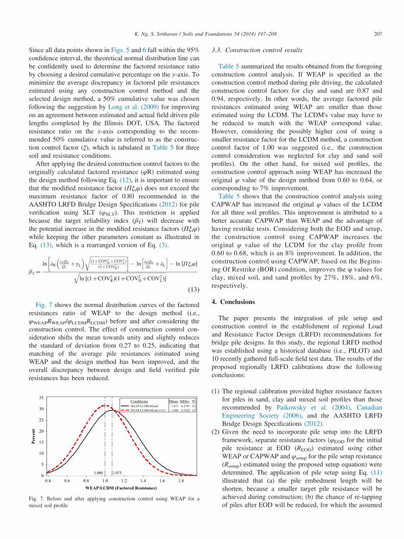
Fig. 7 shows the normal distribution curves of the factoredresistances ratio of WEAP to the design method (i.e.,φWEAPRWEAP/φLCDMRLCDM) before and after considering theconstruction control. The effect of construction control con-sideration shifts the mean towards unity and slightly reducesthe standard of deviation from 0.27 to 0.25, indicating thatmatching of the average pile resistances estimated usingWEAP and the design method has been improved, and theoverall discrepancy between design and field verified pileresistances has been reduced.

1.81.61.41.21.00.80.60.4

35

30

25

20

15

10

5

0

WEAP/LCDM (Factored Resistance)

Perc

ent

1.000 1.073

1.073 0.2707 121.000 0.2522 12

Mean StDev NWEAP/LCDM-MixedWEAP/LCDM-Mixed w/CC

Conditions

Fig. 7. Before and after applying construction control using WEAP for amixed soil profile

3.3. Construction control results

Table 5 summarized the results obtained from the foregoingconstruction control analysis. If WEAP is specified as theconstruction control method during pile driving, the calculatedconstruction control factors for clay and sand are 0.87 and0.94, respectively. In other words, the average factored pileresistances estimated using WEAP are smaller than thoseestimated using the LCDM. The LCDM's value may have tobe reduced to match with the WEAP correspond value.However, considering the possibly higher cost of using asmaller resistance factor for the LCDM method, a constructioncontrol factor of 1.00 was suggested (i.e., the constructioncontrol consideration was neglected for clay and sand soilprofiles). On the other hand, for mixed soil profiles, theconstruction control approach using WEAP has increased theoriginal φ value of the design method from 0.60 to 0.64, orcorresponding to 7% improvement.Table 5 shows that the construction control analysis using

CAPWAP has increased the original φ values of the LCDMfor all three soil profiles. This improvement is attributed to abetter accurate CAPWAP than WEAP and the advantage ofhaving restrike tests. Considering both the EOD and setup,the construction control using CAPWAP increases theoriginal φ value of the LCDM for the clay profile from0.60 to 0.68, which is an 8% improvement. In addition, theconstruction control using CAPWAP, based on the Beginn-ing Of Restrike (BOR) condition, improves the φ values forclay, mixed soil, and sand profiles by 27%, 18%, and 6%,respectively.

4. Conclusions

The paper presents the integration of pile setup andconstruction control in the establishment of regional Loadand Resistance Factor Design (LRFD) recommendations forbridge pile designs. In this study, the regional LRFD methodwas established using a historical database (i.e., PILOT) and10 recently gathered full-scale field test data. The results of theproposed regionally LRFD calibrations draw the followingconclusions:

(1)

The regional calibration provided higher resistance factorsfor piles in sand, clay and mixed soil profiles than thoserecommended by Paikowsky et al. (2004), CanadianEngineering Society (2006), and the AASHTO LRFDBridge Design Specifications (2012).

(2)

Given the need to incorporate pile setup into the LRFDframework, separate resistance factors (φEOD for the initialpile resistance at EOD (REOD) estimated using eitherWEAP or CAPWAP and φsetup for the pile setup resistance(Rsetup) estimated using the proposed setup equation) weredetermined. The application of pile setup using Eq. (11)illustrated that (a) the pile embedment length will beshorten, because a smaller target pile resistance will beachieved during construction; (b) the chance of re-tappingof piles after EOD will be reduced, for which the assumed

K. Ng, S. Sritharan / Soils and Foundations 54 (2014) 197–208208

target pile driving resistance at EOD based on staticanalysis method has not been met; and (c) the economicadvantages of pile setup will be realized while complyingwith the LRFD framework and ensuring a targetreliability level.

(3)

Construction control was integrated into LRFD to mini-mize the discrepancy between design and field pileresistances and to integrate WEAP and CAPWAP as partof the design process. Construction control factors, whichwere calculated using a proposed probabilistic approach,were used as multipliers to the originally calibratedresistance factors of the design method. The considerationof the construction control approach improves the match-ing of the average pile resistances estimated using WEAPor CAPWAP and the design method as well as reducingthe overall discrepancy between design and field verifiedpile resistances. Construction control based on CAPWAPwith the consideration of BOR increased the resistancefactors from 6% to 27%, while the construction controlbased on WEAP only increased the resistance factor from0% to 7%.

Acknowledgments

The authors would like to thank the Iowa Highway ResearchBoard for sponsoring the research presented in this paper. Wewould like to thank the members of the Technical AdvisoryCommittee of this research project for their guidance. Specialthanks are due to Muhannad Suleiman, Matthew Roling, SherifAbdelSalam, and Douglas Wood for their assistances.

References

American Association of State Highway and Transportation Officials(AASHTO), 2003. LRFD Bridge Design Specifications, 2nd editionCustomary U.S. Units, Washington, D.C.

American Association of State Highway and Transportation Officials(AASHTO), 2012. LRFD Bridge Design Specifications 6nd editionCustomary U.S. Units, Washington, D.C. (2013 Interim revisions).

American Society for Testing and Materials (ASTM) D1143, 2007. StandardTest Methods for Deep Foundations under Static Axial Compressive Load.ASTM International, West Conshohocken, PA, USA.

AbdelSalam, S.S., Sritharan, S., Suleiman, M.T., 2010a. Current design andconstruction practices of bridge pile foundations with emphasis onimplementation of LRFD. J. Bridge Eng.: ASCE 15 (6), 749–758.

AbdelSalam, S., Sritharan, S.R.I., Suleiman, T.M., 2011. LRFD resistancefactors for design of driven H-piles in layered soils. J. Bridge Eng.: ASCE16 (6), 739–748.

Allen, T.M., 2005. Development of the WSDOT Pile Driving Formula and itsLRFD Calibration. Washington State Transportation Center, WA (ReportWA-RD 610.1).

Anderson, T.W., Darling, D.A., 1952. Asymptotic theory of certain “goodness-of-fit” criteria based on stochastic processes. Ann. Math. Stat. 23, 193–212.

Barker, R., Duncan, J., Rojiani, K., Ooi, P., Tan, C., Kim, S., 1991. Manualsfor the Design of Bridge Foundations. Transportation Research Board,Washington, D.C. (NCHRP Report 343).

Bloomquist, D., McVay, M., Hu, Z., 2007. Updating Florida Department ofTransportation's (FDOT) Pile/Shaft Design Procedures Based on CPT &DTP Data. Department of Civil and Coastal Engineering, University ofFlorida, Gainesville, FL.

Canadian Engineering Society, 2006. Canadian Foundation EngineeringManual, 4th edition Bitech Publishers Ltd., British Columbia, Canada.

Davisson, M., 1972. High capacity piles, Soil Mechanics Lecture Series onInnovations in Foundation Construction. ASCE, Chicago, IL81–112.

Dirks, K., Kam, P., 1989. Foundation Soils Information Chart. Iowa Depart-ment of Transportation, Office of Road Design, Ames, IA.

Green, D., Ng, K.W., Dunker, K., Sritharan, S., Nop, M., 2012. Developmentof LRFD Design Procedures for Bridge Piles in Iowa – Design Guide andTrack Examples. vol. IV. Institute for Transportation, Iowa State Univer-isty, Ames, IA (Final Report).

Long, James H., Hendrix, Joshua, Baratta, Alma, 2009. Evaluation/Modifica-tion of IDOT Foundation Piling Design and Construction Policy. IllinoisCenter for Transportation, University of Illinois at Urbana-Champaign, IL(Research Report FHWA-ICT-09-037).

Meyerhof, G., 1976. Bearing capacity and settlement of pile foundations.J. Geotech. Eng. Div.: ASCE 102 (GT3), 195–228 (Proc. Paper 11962).

National Highway Institute, 2001. Load and Resistance Factor Design (LRFD)for Highway Bridge Substructures-Reference Manual and ParticipantWorkbook, NHI Course No. 132068, Federal Highway Administration,US Department of Transportation.

Ng, K.W., Suleiman, M.T., Sritharan, S., Roling, M., AbdelSalam, S.S., 2011a.Development of LRFD Design Procedures for Bridge Piles in Iowa – SoilInvestigation and Full-Scaled Pile Tests. vol. II. Institute for Transporta-tion, Iowa State Univeristy, Ames, IA (Final Report).

Ng, K.W., Sritharan, S., Suleiman, T.M., 2011b. Procedure for incorporatingpile setup in load and resistance factor design of steel H-piles in cohesivesoils. In: Transportation Research Board, 90th Annual Meeting, Washing-ton, D.C.

Ng, K.W., Sritharan, S., Dunker, K.F., Danielle, D., 2012. Verification ofrecommended load and resistance factor design approach to pile design andconstruction in cohesive soils. J. Transp. Rec., 2310; 49–58 (Transporta-tion Research Board, Washington, D.C.).

Ng, K.W., Roling, M., AbdelSalam, S.S., Suleiman, M.T., Sritharan, S., 2013a.Pile setup in cohesive soil. I: experimental investigation. J. Geotech.Geoenviron. Eng.: ASCE 139 (2), 199–209.

Ng, K.W., Suleiman, M.T., Sritharan, S., 2013b. Pile setup in cohesive soil. II:analytical quantifications and design recommendations. J. Geotech. Geoen-viron. Eng.: ASCE 139 (2), 210–222.

Nowak, A., 1999. Calibration of LRFD bridge design code. J. Struct. Eng.:ASCE 121 (8), 1245–1251.

Paikowsky, S.G., with Contributions from Birgisson from, Birgisson, B.,McVay, M., Nguyen, T., Kuo, C., Baecher, G., Ayyab, B., Stenersen, K.,O'Malley, K., Chernauskas, L., O'Neill, M., 2004. Load and ResistanceFactor Design (LRFD) for Deep Foundations. Transportation ResearchBoard, Washington, D.C. (NCHRP Report 507).

Pile Dynamics, Inc., 2000. CAPWAP for Windows Manual. Cleveland, OH.Rausche, F., Goble, G.G., Likins, G.E., 1985. Dynamic determination of pile

capacity. J. Geotech. Eng.: ASCE 3 (3), 367–383.Romeu, J.L., 2010. Anderson–Darling: A Goodness of Fit Test for Small

Samples Assumptions. 10. Reliability Analysis Center, Rome, NY(START 2003–5).

Roling, M.J., Sritharan, S., Suleiman, T.M., 2011. Introduction to PILOTdatabase and establishment of LRFD resistance factors for the constructioncontrol of driven steel H-piles. J. Bridge Eng.: ASCE 16 (6), 728–738.

Tomlinson, M.J., 1971. Some effects of pile driving on skin friction. In:Proceeding of the Conference on Behavior of Piles, Institute of CivilEngineers, London, pp. 107–114.