Embed Size (px)
Citation preview

INTEGRATION OF RENEWABLE ENERGY SOURCES:
RELIABILITY-CONSTRAINED POWER SYSTEM PLANNING AND
OPERATIONS USING COMPUTATIONAL INTELLIGENCE
A Dissertation
by
LINGFENG WANG
Submitted to the Office of Graduate Studies ofTexas A&M University
in partial fulfillment of the requirements for the degree of
DOCTOR OF PHILOSOPHY
December 2008
Major Subject: Electrical Engineering

INTEGRATION OF RENEWABLE ENERGY SOURCES:
RELIABILITY-CONSTRAINED POWER SYSTEM PLANNING AND
OPERATIONS USING COMPUTATIONAL INTELLIGENCE
A Dissertation
by
LINGFENG WANG
Submitted to the Office of Graduate Studies ofTexas A&M University
in partial fulfillment of the requirements for the degree of
DOCTOR OF PHILOSOPHY
Approved by:
Chair of Committee, Chanan SinghCommittee Members, Karen L. Butler-Purry
Jim X. JiLewis Ntaimo
Head of Department, Costas N. Georghiades
December 2008
Major Subject: Electrical Engineering

iii
ABSTRACT
Integration of Renewable Energy Sources: Reliability-constrained Power System
Planning and Operations Using Computational Intelligence. (December 2008)
Lingfeng Wang, B.Eng, Zhejiang University, China;
M.Eng, Zhejiang University, China;
M.Eng, National University of Singapore
Chair of Advisory Committee: Dr. Chanan Singh
Renewable sources of energy such as wind turbine generators and solar panels
have attracted much attention because they are environmentally friendly, do not
consume fossil fuels, and can enhance a nation’s energy security. As a result, recently
more significant amounts of renewable energy are being integrated into conventional
power grids. The research reported in this dissertation primarily investigates the
reliability-constrained planning and operations of electric power systems including
renewable sources of energy by accounting for uncertainty. The major sources of
uncertainty in these systems include equipment failures and stochastic variations in
time-dependent power sources.
Different energy sources have different characteristics in terms of cost, power
dispatchability, and environmental impact. For instance, the intermittency of some
renewable energy sources may compromise the system reliability when they are inte-
grated into the traditional power grids. Thus, multiple issues should be considered in
grid interconnection, including system cost, reliability, and pollutant emissions. Fur-
thermore, due to the high complexity and high nonlinearity of such non-traditional
power systems with multiple energy sources, computational intelligence based opti-
mization methods are used to resolve several important and challenging problems in
their operations and planning. Meanwhile, probabilistic methods are used for relia-

iv
bility evaluation in these reliability-constrained planning and design.
The major problems studied in the dissertation include reliability evaluation of
power systems with time-dependent energy sources, multi-objective design of hybrid
generation systems, risk and cost tradeoff in economic dispatch with wind power pen-
etration, optimal placement of distributed generators and protective devices in power
distribution systems, and reliability-based estimation of wind power capacity credit.
These case studies have demonstrated the viability and effectiveness of computational
intelligence based methods in dealing with a set of important problems in this research
arena.

v
To my family and friends

vi
ACKNOWLEDGMENTS
Many people deserve special acknowledgment for their support throughout the
duration of this work.
First, I must acknowledge my deep gratitude to my advisor, Dr. Chanan Singh,
for his excellent professional guidance and constant assistance rendered in making this
dissertation possible. His insightful comments and suggestions fueled the research. I
want to say that working under his supervision during my Ph.D. study is one of the
luckiest things in my life. His mentoring will benefit me in a long term.
Next, I would like to express great thanks to Dr. Karen Butler-Purry, Dr. Jim
Ji, and Dr. Lewis Ntaimo for their effort in serving as members of my Ph.D. studies
committee. They consistently provided strong support to my career development in
the academic environment. I really appreciate their help during these years.
I am indebted to many friends for their assistance and advice. They have stood
by and encouraged me when my productivity waned. I also wish to thank my family
for their ever-present encouragement and for the moral and practical support given
over the years before and throughout this endeavor. I dedicate this dissertation to
them.

vii
TABLE OF CONTENTS
CHAPTER Page
I INTRODUCTION . . . . . . . . . . . . . . . . . . . . . . . . . . 1
A. Introduction . . . . . . . . . . . . . . . . . . . . . . . . . . 1
B. Research Objectives . . . . . . . . . . . . . . . . . . . . . . 2
C. Organization of Dissertation . . . . . . . . . . . . . . . . . 3
II CONVENTIONAL AND RENEWABLE SOURCES OF ENERGY 4
A. Fuel-Fired Generators . . . . . . . . . . . . . . . . . . . . . 5
B. Wind Turbine Generators . . . . . . . . . . . . . . . . . . 6
C. Photovoltaic Cells . . . . . . . . . . . . . . . . . . . . . . . 7
D. Storage Batteries . . . . . . . . . . . . . . . . . . . . . . . 7
E. Other Alternative Sources . . . . . . . . . . . . . . . . . . 8
1. Tidal power . . . . . . . . . . . . . . . . . . . . . . . . 8
2. Biomass . . . . . . . . . . . . . . . . . . . . . . . . . . 8
3. Hydrogen and fuel cells . . . . . . . . . . . . . . . . . 8
4. Geothermal energy . . . . . . . . . . . . . . . . . . . . 9
III RELIABILITY-CONSTRAINED POWER SYSTEM PLAN-
NING AND OPERATIONS INCLUDING TIME-DEPENDENT
ENERGY SOURCES . . . . . . . . . . . . . . . . . . . . . . . . 10
A. Generation System Reliability Including Renewable En-
ergy Sources . . . . . . . . . . . . . . . . . . . . . . . . . . 11
B. Distribution System Reliability Including Renewable En-
ergy Sources . . . . . . . . . . . . . . . . . . . . . . . . . . 13
IV COMPUTATIONAL INTELLIGENCE BASED OPTIMIZA-
TION METHODS . . . . . . . . . . . . . . . . . . . . . . . . . . 16
A. Genetic Algorithms . . . . . . . . . . . . . . . . . . . . . . 17
B. Particle Swarm Optimization . . . . . . . . . . . . . . . . 19
C. Ant Colony Optimization . . . . . . . . . . . . . . . . . . . 23
D. Artificial Immune Systems . . . . . . . . . . . . . . . . . . 25
V POPULATION-BASED INTELLIGENT SEARCH IN RE-
LIABILITY EVALUATION OF HYBRID GENERATION
SYSTEMS WITH WIND POWER PENETRATION . . . . . . 28

viii
CHAPTER Page
A. Introduction . . . . . . . . . . . . . . . . . . . . . . . . . . 29
B. Reliability Evaluation of Hybrid Generating Systems . . . 31
C. Monte Carlo Simulation and Population-based Intelli-
gent Search . . . . . . . . . . . . . . . . . . . . . . . . . . 32
1. State space . . . . . . . . . . . . . . . . . . . . . . . . 33
2. Monte Carlo Simulation . . . . . . . . . . . . . . . . . 34
a. Computational procedure . . . . . . . . . . . . . 35
b. Stopping criteria . . . . . . . . . . . . . . . . . . 36
c. Some remarks . . . . . . . . . . . . . . . . . . . . 36
3. Population-based Intelligent Search . . . . . . . . . . . 37
a. Computational procedure . . . . . . . . . . . . . 37
b. Stopping criteria . . . . . . . . . . . . . . . . . . 38
c. Some remarks . . . . . . . . . . . . . . . . . . . . 39
d. Representative PIS algorithms . . . . . . . . . . . 39
4. Conceptual comparison between MCS and PIS . . . . 40
D. PIS-based Adequacy Evaluation . . . . . . . . . . . . . . . 41
E. Simulations and Evaluation . . . . . . . . . . . . . . . . . 48
F. Summary . . . . . . . . . . . . . . . . . . . . . . . . . . . 58
VI RELIABILITY-CONSTRAINED OPTIMUM PLACEMENT
OF RECLOSERS AND DISTRIBUTED GENERATORS IN
DISTRIBUTION NETWORKS USING ANT COLONY SYS-
TEM ALGORITHM . . . . . . . . . . . . . . . . . . . . . . . . 59
A. Introduction . . . . . . . . . . . . . . . . . . . . . . . . . . 59
B. Problem Formulation . . . . . . . . . . . . . . . . . . . . . 60
C. Ant Colony System Algorithms . . . . . . . . . . . . . . . 62
1. Basic principle . . . . . . . . . . . . . . . . . . . . . . 63
2. Basic steps . . . . . . . . . . . . . . . . . . . . . . . . 63
D. The Proposed Approach . . . . . . . . . . . . . . . . . . . 65
1. Search space . . . . . . . . . . . . . . . . . . . . . . . 66
2. Reliability evaluation . . . . . . . . . . . . . . . . . . 67
3. Solution construction and pheromone updating . . . . 68
4. Computational procedure . . . . . . . . . . . . . . . . 69
E. Simulation Results and Analysis . . . . . . . . . . . . . . . 70
F. Summary . . . . . . . . . . . . . . . . . . . . . . . . . . . 78

ix
CHAPTER Page
VII RISK AND COST TRADEOFF IN ECONOMIC DISPATCH
INCLUDING WIND POWER PENETRATION BASED ON
MULTI-OBJECTIVE MEMETIC PARTICLE SWARM OP-
TIMIZATION . . . . . . . . . . . . . . . . . . . . . . . . . . . . 86
A. Introduction . . . . . . . . . . . . . . . . . . . . . . . . . . 87
B. Wind Power Penetration Model . . . . . . . . . . . . . . . 88
C. Problem Formulation . . . . . . . . . . . . . . . . . . . . . 92
1. Problem objectives . . . . . . . . . . . . . . . . . . . . 92
2. Problem constraints . . . . . . . . . . . . . . . . . . . 94
3. Problem statement . . . . . . . . . . . . . . . . . . . . 95
D. The Proposed Approach . . . . . . . . . . . . . . . . . . . 96
1. Multi-objective PSO framework . . . . . . . . . . . . . 97
2. Archiving . . . . . . . . . . . . . . . . . . . . . . . . . 100
3. Global best selection . . . . . . . . . . . . . . . . . . . 101
4. Local search . . . . . . . . . . . . . . . . . . . . . . . 102
5. Constraints handling . . . . . . . . . . . . . . . . . . . 103
6. Individual (particle) representation . . . . . . . . . . . 104
7. Algorithm steps . . . . . . . . . . . . . . . . . . . . . 104
E. Simulation and Evaluation of the Proposed Approach . . . 108
1. Comparison of different design scenarios . . . . . . . . 109
2. Sensitivity analysis . . . . . . . . . . . . . . . . . . . . 112
3. Comparative studies . . . . . . . . . . . . . . . . . . . 114
F. Summary . . . . . . . . . . . . . . . . . . . . . . . . . . . 120
VIII MULTI-CRITERIA DESIGN OF HYBRID POWER GEN-
ERATION SYSTEMS BASED ON A MODIFIED PARTI-
CLE SWARM OPTIMIZATION ALGORITHM . . . . . . . . . 122
A. Introduction . . . . . . . . . . . . . . . . . . . . . . . . . . 122
B. Problem Formulation . . . . . . . . . . . . . . . . . . . . . 125
1. Design objectives . . . . . . . . . . . . . . . . . . . . . 126
2. Design constraints . . . . . . . . . . . . . . . . . . . . 130
3. Problem statement . . . . . . . . . . . . . . . . . . . . 132
4. Operation strategies . . . . . . . . . . . . . . . . . . . 133
C. The Proposed Approach . . . . . . . . . . . . . . . . . . . 133
1. CMIMOPSO . . . . . . . . . . . . . . . . . . . . . . . 133
2. Representation of candidate solutions . . . . . . . . . 135
3. Data flow of the optimization procedure . . . . . . . . 135

x
CHAPTER Page
D. A Case Study: System Design Without Incorporating
Uncertainties . . . . . . . . . . . . . . . . . . . . . . . . . 137
1. System parameters . . . . . . . . . . . . . . . . . . . . 137
2. PSO parameters . . . . . . . . . . . . . . . . . . . . . 138
3. Simulation results . . . . . . . . . . . . . . . . . . . . 139
4. Sensitivity to system parameters . . . . . . . . . . . . 139
E. Adequacy-constrained Design Incorporating System Un-
certainties . . . . . . . . . . . . . . . . . . . . . . . . . . . 140
1. Problem formulation . . . . . . . . . . . . . . . . . . . 142
2. Simulation results . . . . . . . . . . . . . . . . . . . . 143
F. Summary . . . . . . . . . . . . . . . . . . . . . . . . . . . 145
IX CAPACITY CREDIT ESTIMATION OF WIND POWER:
FORMULATION AS AN OPTIMIZATION PROBLEM . . . . . 150
A. Introduction . . . . . . . . . . . . . . . . . . . . . . . . . . 150
B. Wind Power Capacity Credit . . . . . . . . . . . . . . . . . 152
C. The Proposed Method . . . . . . . . . . . . . . . . . . . . 153
1. Problem formulation . . . . . . . . . . . . . . . . . . . 153
2. Computational procedure . . . . . . . . . . . . . . . . 154
D. A Numerical Example . . . . . . . . . . . . . . . . . . . . 155
E. Summary . . . . . . . . . . . . . . . . . . . . . . . . . . . 156
X CONCLUSIONS AND OUTLOOK . . . . . . . . . . . . . . . . 157
A. Conclusions . . . . . . . . . . . . . . . . . . . . . . . . . . 157
B. Outlook . . . . . . . . . . . . . . . . . . . . . . . . . . . . 160
REFERENCES . . . . . . . . . . . . . . . . . . . . . . . . . . . . . . . . . . . 163
VITA . . . . . . . . . . . . . . . . . . . . . . . . . . . . . . . . . . . . . . . . 174

xi
LIST OF TABLES
TABLE Page
I Reliability indices for unconventional capacity 100 MW . . . . . . . . 51
II Reliability indices for unconventional capacity 200 MW . . . . . . . . 51
III Reliability indices for unconventional capacity 400 MW. . . . . . . . 52
IV Growth of reliability indices with the increasing generations . . . . . 52
V Comparison of sampling efficiency of different PIS algorithms in
the entire optimization process. . . . . . . . . . . . . . . . . . . . . . 54
VI No distributed generators in the distribution system (test system 1) . 72
VII Maximum power of each distributed generator = 0.3 MW (test
system 1) . . . . . . . . . . . . . . . . . . . . . . . . . . . . . . . . . 73
VIII Maximum power of each distributed generator = 0.5 MW (test
system 1) . . . . . . . . . . . . . . . . . . . . . . . . . . . . . . . . . 74
IX Maximum power of each distributed generator = 1.0 MW (test
system 1) . . . . . . . . . . . . . . . . . . . . . . . . . . . . . . . . . 75
X Design scenarios where GA and ACS have different results (test
system 1) . . . . . . . . . . . . . . . . . . . . . . . . . . . . . . . . . 76
XI Comparison of different results obtained from GA and ACS (test
system 1) . . . . . . . . . . . . . . . . . . . . . . . . . . . . . . . . . 77
XII Maximum power of each distributed generator = 0.3 MW (test
system 2) . . . . . . . . . . . . . . . . . . . . . . . . . . . . . . . . . 78
XIII Maximum power of each distributed generator = 0.5 MW (test
system 2) . . . . . . . . . . . . . . . . . . . . . . . . . . . . . . . . . 78
XIV Maximum power of each distributed generator = 0.7 MW (test
system 2) . . . . . . . . . . . . . . . . . . . . . . . . . . . . . . . . . 79

xii
TABLE Page
XV Design scenarios where GA and ACS have different results (test
system 2) . . . . . . . . . . . . . . . . . . . . . . . . . . . . . . . . . 80
XVI Comparison of different results obtained from GA and ACS (test
system 2) . . . . . . . . . . . . . . . . . . . . . . . . . . . . . . . . . 85
XVII Fuel cost coefficients and generator capacities . . . . . . . . . . . . . 109
XVIII Example solutions for different design scenarios. . . . . . . . . . . . . 112
XIX Comparison of C-metric for different algorithms . . . . . . . . . . . . 117
XX Comparison of the spacing metric for different algorithms . . . . . . 117
XXI Comparison of the error ratio metric for different algorithms . . . . . 118
XXII Comparison of computational time for different algorithms (in seconds) 119
XXIII The data used in the simulation program . . . . . . . . . . . . . . . . 148
XXIV Two illustrative non-dominated solutions for tri-objective optimization 149
XXV Two illustrative system configurations for adequacy-constrained design 149
XXVI Two illustrative system configurations for adequacy-constrained
design with load forecasting . . . . . . . . . . . . . . . . . . . . . . . 149

xiii
LIST OF FIGURES
FIGURE Page
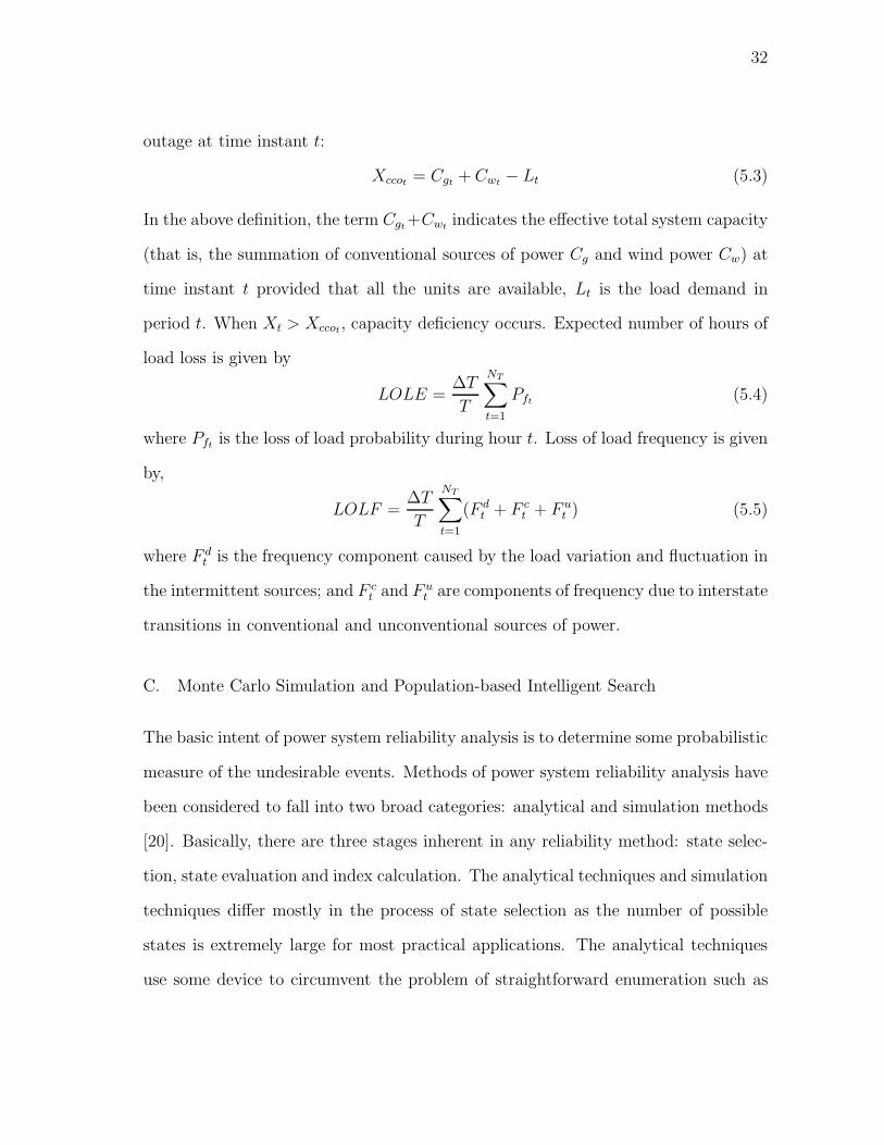
1 Classification of system states in the whole state space . . . . . . . . 33
2 Individual (i.e., system-state) representation . . . . . . . . . . . . . . 42
3 Ratio of meaningful states and total sampled states . . . . . . . . . . 55
4 Distributed generation-enhanced radial feeder . . . . . . . . . . . . . 61
5 Search space of the problem . . . . . . . . . . . . . . . . . . . . . . . 67
6 Flow chart for calculating system reliability of each recloser configuration 81
7 Computational procedure for the proposed algorithm. . . . . . . . . . 82
8 One-line diagram of the 69-bus test distribution system . . . . . . . . 83
9 One-line diagram of the 394-bus test distribution system [47] . . . . . 84
10 Fuzzy linear representation of the security level in terms of wind
penetration and wind power cost. . . . . . . . . . . . . . . . . . . . . 89
11 Fuzzy quadratic representation of the security level in terms of
wind power penetration . . . . . . . . . . . . . . . . . . . . . . . . . 91
12 Fuzzy quadratic representation of the security level in terms of
wind power cost . . . . . . . . . . . . . . . . . . . . . . . . . . . . . 91
13 Data flow diagram of the proposed algorithm . . . . . . . . . . . . . 105
14 IEEE 30-bus test power system . . . . . . . . . . . . . . . . . . . . . 108
15 Different curve shapes of membership functions . . . . . . . . . . . . 111
16 Pareto fronts obtained based on different membership functions . . . 113
17 Pareto fronts obtained for different wind penetration ranges . . . . . 114

xiv
FIGURE Page
18 Pareto fronts obtained for different running costs of wind power . . . 115
19 Configuration of a typical hybrid generation system . . . . . . . . . . 125
20 Hourly mean wind speed, insolation, and load profiles . . . . . . . . . 138
21 Pareto fronts for bi- and tri-objective optimization scenarios . . . . . 139
22 Pareto fronts obtained from different mean wind speeds . . . . . . . 140
23 Pareto fronts obtained from different economic rates . . . . . . . . . 141
24 Pareto front indicating a set of non-inferior design solutions . . . . . 144
25 Impacts of different wind speeds on Pareto fronts derived . . . . . . . 145
26 Impacts of different insolations on Pareto fronts derived . . . . . . . 146
27 Pareto front indicating a set of non-inferior design solutions con-
sidering stochastic load variations . . . . . . . . . . . . . . . . . . . . 147
28 Impacts of different wind speeds on Pareto fronts derived consid-
ering stochastic load variations . . . . . . . . . . . . . . . . . . . . . 147
29 Dataflow diagram of PSO-based WPCC estimation . . . . . . . . . . 154

1
CHAPTER I
INTRODUCTION
This chapter first presents the background of the research reported in this dissertation.
Then research objectives and the dissertation organization are given outlining an
overall picture of this investigation.
A. Introduction
The optimum economic planning and operation of electric power systems play an
important role in the modern electric power industry. In the face of depleting nat-
ural resources, the efficient use of available energy sources is becoming increasingly
important in reducing operational costs while satisfying ever-tighter pollution regula-
tions. Meanwhile, reliability analysis of the power system is being incorporated into
various planning and operation strategies. Furthermore, in the recent years, renew-
able sources of energy have attracted much attention. They are highly advantageous
with respect to the traditional fossil fuels in some respects. For instance, they are
environmentally benign and do not consume depleting fuel reserves. However, some
renewable sources of energy such as wind turbine generators and solar panels are
time-dependent. This means that their availability in each time period cannot be
precisely predicted ahead of time. As a result, when this type of energy sources is in-
tegrated into conventional power grids, some reliability problems may be introduced.
For instance, when the wind speed drops, power deficiency may be caused in some
regions due to insufficient generation and this may lead to power outage. Therefore,
reliability issues in this type of power systems should be carefully addressed.
The journal model is IEEE Transactions on Automatic Control.

2
This research is intended to improve the utilization of natural resources, minimize
the environmental pollution, and ensure the power system reliability. With the pene-
tration of more significant amounts of time-dependent energy sources, more uncertain
factors are involved in system reliability evaluation including equipment failures and
stochastic characteristic of generation sources. For this purpose, probabilistic meth-
ods are used for reliability evaluation by taking into account various uncertainties.
Meanwhile, power networks have become very large these days which involve numer-
ous nodes and lines. As a result, traditional analytical methods oftentimes become
less effective or even are unable to deal with these kinds of complex power systems.
In this work, computational intelligence based optimization techniques are applied to
deal with a set of challenging problems, which are usually able to derive an adequate
solution within a reasonable amount of time. These methods are less sensitive to the
system complexity and nonlinearity as compared with the analytical methods. In this
study, several important real-world problems in this research arena are examined.
B. Research Objectives
As indicated in the dissertation title, there are three major research objectives in this
study, which are to be examined through several case studies.
• The impact of renewable energy integration on the traditional power systems,
especially from the perspective of system planning and operations.
• Reliability-constrained designs accounting for renewable energy integration, es-
pecially time-dependent energy sources.
• Effectiveness of computational intelligence based optimization methods in deal-
ing with highly complex and highly nonlinear problems in power system plan-
ning and operations.

3
C. Organization of Dissertation
The dissertation can be broadly divided into two parts. The first four chapters present
the background knowledge and motivation of this research, and the following four
chapters are devoted to several important problems in this research arena. In the
second chapter, some conventional and renewable sources of energy are presented
focusing on their cost and environmental impact. The third chapter discusses the
reliability-constrained planning and operations when the renewable energy is inte-
grated into the power grids at both power generation and distribution levels. Chapter
IV presents the major computational intelligence based optimization techniques used
in this study. In Chapter V, reliability evaluation of hybrid generation systems is
carried out based on population-based intelligent search, where the stochastic nature
of wind power is also taken into account. In Chapter VI, the optimum placement
schemes of distributed generators and reclosers for power distribution networks are
derived by an outstanding discrete optimizer termed ant colony system. In Chap-
ter VII, the economic power dispatch problem is readdressed when the wind power
is integrated. An improved particle swarm optimization algorithm is developed to
find out a set of tradeoff solutions in terms of operational cost and system security.
Chapter VIII discusses the optimal design of hybrid generation systems including
fossil-fuel-fired generators, wind turbine generators, solar panels, and storage bat-
teries. A modified multi-objective particle swarm optimization algorithm is used to
derive the tradeoff solutions measured by system cost, reliability, and pollutants emis-
sion. In Chapter IX, the wind power capacity credit is estimated through a particle
swarm optimization algorithm. Loss of load probability is used as the reliability index
in the calculation.

4
CHAPTER II
CONVENTIONAL AND RENEWABLE SOURCES OF ENERGY
Due to the ever-increasing demands on energy, energy consumption worldwide is
rapidly increasing. As a result, fossil-fuel reserves are depleting and energy prices are
skyrocketing especially in the past few years. Meanwhile, with increasing concerns
on environmental protection, there are stricter regulations on pollutant emissions.
The most important emissions considered in the power generation industry, due to
their highly damaging effects on the ecological environment, are sulfur dioxide and
nitrogen oxides. These emissions can be modeled through functions that associate
emissions with power production for conventional generating units. Besides environ-
mental pollution, global warming is another issue of much concern internationally in
the current political climate, and it has become a highly pressing challenge. Human
activity has been aggravating the emission of greenhouse gases, because the major
portion of carbon dioxide is produced by combusting coal, oil, and gas. As a severe
consequence, earth surface temperature has increased around 0.6C since the late 19th
century, and about 0.2C to 0.3C within the past 25 years (from National Oceanic
and Atmospheric Administration). However, the consumption of electric power keeps
growing dramatically on a worldwide basis. Many countries have specified goals to
curb the emission of carbon dioxide to prevent or slow down further global warming.
Basically, there are two major ways to achieve this goal, that is, implementing energy-
saving measures and wide utilization of renewable energy. The renewable sources of
energy have a much lower environmental impact than conventional energy sources,
producing low or no emissions of carbon dioxide, particulates, and sulphur dioxide.
As said earlier, today we are also facing the environmental crisis caused by climate
change and greenhouse/polluting gas emissions. Development of renewable energy

5
technologies will not only make energy independence feasible, but it will protect our
Earth home and provide healthier environments for human beings. Nowadays, people
from relevant fields are bringing a broad range of expertise to radically increase the
utilization of renewable energy and alternative fuels. Most renewable energy comes
directly or indirectly from the sun, thus, the energy resource will not be depleted
in the foreseeable future. Furthermore, the energy security of a country can be sig-
nificantly enhanced by fully utilizing renewable energy due to its decreased reliance
on imported fossil fuels. In this section, the characteristics of several alternative
sources of energy are discussed. Besides the traditional fuel-fired generation, renew-
able sources of energy including wind turbine generators, solar panels, wave and tidal
power, biomass, fuel cells, and geothermal energy are discussed in this section.
A. Fuel-Fired Generators
Most of the world energy consumption currently relies on conventional sources of en-
ergy including coal, oil, and natural gas. These fossil fuels are nonrenewable since
they consume limited resources that are diminishing, becoming too cost-ineffective, or
too environmentally detrimental to retrieve. In traditional FFGs, pollutant emissions
are the major drawback. For instance, coal has been a reliable, abundantly available,
and relatively inexpensive fuel source for a long time, but coal-fired power genera-
tion is facing increasing pressure since environmental regulations are becoming more
stringent than ever around the world. An affordable control scheme for air pollution
reduction is a deciding factor in fossil fuels continued role as a prime energy source
in the power generation industry. As a result, combined use of fuel sources and other
cleaner sources may be a viable way to abate pollutant emissions while still fulfilling
certain cost and reliability requirements. In the restructured power market, DG using

6
renewable sources of energy is being connected to the utility grid at the distribution
level, attempting to diminish the demerits in traditional central generation plants.
Renewable power sources promise to play an important role in complementing the
fossil-fuel-fired generation by reducing its negative environmental impacts.
B. Wind Turbine Generators
Wind energy is ample, renewable, widely dispersed, and clean. The conversion of
wind energy into electricity can be achieved using wind turbines installed onshore and
offshore. It can be used by large-scale wind farms for nation-level power grids as well
as small turbines for rural residences or grid-isolated locations. WTGs are powered by
windmills, which are usually operated by utilities and independent power producers
(IPPs). They are located in areas with rich wind resources onshore or offshore.
Thus, effective utilization of wind energy is particularly attractive in spurring the
reduction of pollutant emissions, which is a major drawback to the traditional fossil-
fuel-based generation. However, the availability of wind power is primarily determined
by weather conditions and thus can quite fluctuate in a year or even in a day. The
volatility of wind power should be fully addressed when designing a renewable-based
power plant. In our investigation, other power sources are also used in order to
mitigate or even out the fluctuations caused by the intermittency of wind power.
Wind power has been widely developed worldwide. For instance, the average U.S.
wind energy growth rate for the past 5 years is 24%. The leading countries in wind
power generation are Germany, Spain, Denmark, and the Netherlands, and they
occupy 84% of the total European wind capacity. By year 2020, it is anticipated that
wind power will fulfill the residential demands of about half of the region’s population.

7
C. Photovoltaic Cells
Sunlight can be directly converted into electric energy by PV panels. PV panels
use the photovoltaic effect of semiconductors to generate electricity from sunlight.
Like wind power, the production of a solar system is also influenced considerably
by varying meteorological conditions. Because of its intermittent power supply, other
supplemental power sources such as storage batteries are usually needed to smooth out
the fluctuations. PV panels produce no direct emissions and thus are environmentally
friendly. The advance of manufacturing technologies has significantly reduced the cost
of a PV system, and PVs also have lower maintenance demands. Several PV power
plants with capacities of 300 to 500 kW have been linked to power grids in Europe and
the United States, and extensive research is now underway to achieve less expensive
but more efficient PV cells.
D. Storage Batteries
Since both WTGs and PVs are intermittent sources of power, it is highly desirable
to incorporate energy storage into such hybrid power systems. Energy storage can
smooth out the fluctuations of wind and solar power and improve the load availability.
In a certain sense, storage batteries can be deemed a buffer to balance the supply-
and-demand relationship. When the power generated by WTGs and PVs exceeds
the load demand, a certain amount of surplus power will be stored in the batteries
within their total storage capacity for future use. On the contrary, when there is any
deficiency in overall power generation, the stored power will be used to supply the
load so as to enhance system reliability. Energy storage reduces the power dumped
and thus helps to minimize the operational cost.

8
E. Other Alternative Sources
1. Tidal power
Tidal power is produced by capturing the energy contained in moving water mass
due to strong waves or tides, and it has a fairly high efficiency rate. Like other
renewable sources of energy, it requires a high capital cost but fairly low operation
and maintenance costs. However, the installation of a barrage may significantly affect
the water inside the basin as well as hamper fish activities. Among all kinds of
intermittent renewable sources, tidal power is deemed capable of supplying relatively
continuous and predictable power and is anticipated to increase considerably in the
upcoming years.
2. Biomass
In general, biomass refers to plant matter grown for use as biofuel as well as biodegrad-
able wastes that can be combusted as fuel. It primarily includes solids, biofuels, bio-
gas, landfill gas, and sewage treatment plant gas. Biomass is a type of sustainable
energy but still contributes to global warming. If directly combusted without taking
proper emissions filtering measures, it will cause environmental pollution problems
as well. Based on the current technologies, production of liquid fuels from biomass
is not sufficiently cost-effective due to the expenses caused by biomass production
coupled with its conversion procedure to alcohols. By 2030, biomass-fueled electric
power is expected to triple and meet 2% of the total world energy demand.
3. Hydrogen and fuel cells
More recently, the fuel cell has been applauded as the “microchip of the energy
industry” due to its great promise as an alternative for clean power generation. A

9
fuel cell is fundamentally an electrochemical device capable of converting hydrogen
and oxygen into water, meanwhile producing electricity. Salient features of fuel cells
are that they neither produce harmful emissions nor consume oil. Fuel cells are
particularly useful in serving as power sources in remote locations or isolated areas
such as spacecrafts and rural regions. They can also be applied to baseload power
supply, combined heat and power generation, electric and hybrid electric vehicles,
off-grid power generation, and so forth.
4. Geothermal energy
Geothermal can be interpreted as “earth heat” in plain text, and it can be used for
clean power generation. Geothermal power is more competitive in countries that have
restricted fossil-fuel resources. Geothermal energy for electricity generation has grown
rapidly worldwide, reaching about 8,000 MW. Recent high and wildly fluctuating
power prices have made geothermal energy more economically attractive.
Due to space restrictions, other alternative sources of energy such as hydropower
and biofuels will not be discussed here. Corresponding literature may be referred to
for more details. In this dissertation, the focus is put on the time-dependent energy
sources such as wind power and solar power, which may have significant impacts on
the power system reliability in grid integration.

10
CHAPTER III
RELIABILITY-CONSTRAINED POWER SYSTEM PLANNING AND
OPERATIONS INCLUDING TIME-DEPENDENT ENERGY SOURCES
System designers and planners always have concerns about system reliability. The
term reliability relates to the ability of a system to perform its intended function for
a given period of time under stated environmental conditions. The general approach
has been, however, either intuitive or based on rule-of-thumb criteria derived from
previous experience with similar systems. The intuitive approach has turned out to be
inadequate due to the large scale and high complexity of modern industrial systems,
where a composite of equipment and skills function as a unified entity. In the past two
decades, more sophisticated quantitative techniques and indices have been developed
to respond meaningfully to factors that affect system reliability. Quantitative assess-
ment is achieved by building mathematical models that reasonably approximate the
actual system and can be manipulated to derive suitable reliability measures. When
quantitatively defined, reliability becomes a parameter that can be traded off with
other parameters. The necessity of quantitative reliability springs from the ever in-
creasing complexity of systems, cost competitiveness, alternative design evaluations,
cost-benefit analysis, the need to study effects of operation and maintenance proce-
dures, and so forth. Reliability modeling and evaluation is an important component
in any reliability analysis program because the selected model provides the basis for
predicting reliability measures [1], [2]. Various techniques of reliability modeling and
evaluation can be classified into direct analytical modeling or simulation or a mixture
of the two approaches. In the direct analytical modeling method, a model is built that
reasonably approximates the physical system and is also amenable to calculation. The
reliability measures are then attained by manipulating the model. Simulation also

11
deploys a mathematical model but proceeds by carrying out sampling experiments
on this model. It is more flexible but is also more time-consuming and less accurate.
Simulation can be used to provide estimates of the reliability measures. Monte Carlo
simulation is a representative simulation method that is usually adopted to deal with
reliability evaluation of large-scale or complex power systems [3]. Also, more recently,
artificial intelligence based reliability evaluation has shown its promise in improving
evaluation efficiency [4].
A. Generation System Reliability Including Renewable Energy Sources
The objective of electric power systems is to supply electrical energy to consumers at
low cost while simultaneously providing acceptable or economically justifiable service
quality. Generation adequacy deals with the relative ability of the system to supply
system load considering that generating units may be out of service when needed due
to planned or unplanned outages or that the basic energy sources may be inadequate.
Generation “adequacy” is distinct from the concept of “security,” which deals with
the relative ability of the system to survive sudden shocks or upsets such as faults
or equipment failures without cascading failures or loss of stability. Generation ad-
equacy is usually measured through the use of some adequacy index that quantifies
system adequacy performance, and it is enforced through a criterion based on an ac-
ceptable value of this adequacy index. Some utilities rely on adequacy criteria whose
values have been chosen based on engineering judgment to yield a reasonable bal-
ance between system cost and reliability performance and that have been validated
by historical experience. However, if adequacy criteria are based on probabilistic in-
dices that bear reasonable relationships to the actual reliability performance of the
system, more pragmatic methods may be used to decide appropriate values of the

12
criteria. The reliability indices of generation capacity adequacy assessment can be
broadly divided into two categories: deterministic and probabilistic. Deterministic in-
dices normally include a percentage reserve margin as well as reserve margin in terms
of the largest unit. Probabilistic indices usually comprise loss of load expectation
(LOLE), frequency and duration (F&D) of capacity shortage events, and expected
unserved energy (EUE). LOLE on an hourly basis is the expected number of hours
per year when insufficient generating capacity is available to serve the load. It does
not give information on a number of important system reliability attributes including
magnitude of capacity shortages, duration of capacity shortage events, and expected
amount of unserved energy. Frequency of generating capacity shortage events is de-
fined as the expected number of such events per year. Duration is the expected
length of capacity shortage periods when they occur. F&D indices use hourly load
information and thus reflect the influences of daily load cycle shape. F&D methods
model unit parameters more comprehensively than those models used in LOLE. F&D
indices are conceptually superior with respect to LOLE. However, they have greater
data requirements. The EUE index measures the expected amount of energy that will
fail to be supplied per year due to generating capacity differences and/or shortages
in basic energy supplies. Reliability analysis of power generation systems including
time-dependent sources is aggravated by the volatile nature of wind resources, and
thus the evaluation process unavoidably becomes more complex and challenging. The
generating adequacy may be compromised provided that there is insufficient power
available to fulfill the load due to intermittency of renewable sources of power. In the
hybrid generation system design, besides the impact caused by generation volatility,
the uncertainties including equipment failures coupled with random variations in both
generation and load should all be considered. Usually time-series models can be used
to accomplish generation and load forecasting by accounting for the randomness of

13
renewable sources of energy and load demands.
A system state depends on the combination of all component states and each
component state can be characterized by the probability that the component appears
in that state. Adequacy evaluation of power generation systems is usually concerned
with assessing the capability of generation facilities to fulfill the system load require-
ments. In this assessment, the associated transmission and distribution facilities are
deemed to be completely reliable and capable of transmitting and distributing the
generated energy to the customer load points without failure possibility. Reliability
indices of a generating system can be seen as the expected value of a test function
applied to a system state, which is a vector representing the state of each component,
in order to find out whether the specific generation combination corresponds to a fea-
sible or infeasible solution. Thus, a fundamental parameter in reliability evaluation
is the mathematical expectation of a given reliability index. Reliability evaluation is
discussed from an expectation point of view in this study.
In this dissertation, four projects are concerned about the impacts of intermit-
tent renewable energy sources on the power generation systems. They are reliability
evaluation for hybrid generation systems including wind power penetration, economic
power dispatch including wind power, optimum designs of hybrid power generation
systems including multiple renewable energy sources, and reliability-based estimation
of wind power capacity credit.
B. Distribution System Reliability Including Renewable Energy Sources
Distributed generation (DG) is also known as embedded generation or dispersed gen-
eration, which is a hot topic in both academia and industry in recent years [5]. In
the restructured power industry environment, distributed generation using renewable

14
energy sources is becoming increasingly important. Distributed generators are being
directly connected to the power distribution networks, most often for enhancing the
power system reliability in the presence of system faults and insufficient generation,
or reducing the environmental impacts by avoiding use of fossil fuels.
However, interconnection of renewable energy sources to the existing distribution
networks poses great challenges. The power flow in this type of power systems is bi-
directional, which is significantly different from the traditional power distribution
networks. The major concern of distribution network operators (DNOs) nowadays
is the damaging impacts on power quality of the main power grid caused by the
connected DGs. Thus, the coordination and control of protective devices should be
redesigned. Moreover, the adverse impacts caused by the high degree penetration of
alternative sources of energy should be taken care of.
As said earlier, when DGs are connected to the main power grid, one of the
objectives is to enhance the system reliability. For instance, they can supply extra
power to the power grid to minimize the loss of load probability; meanwhile, they
can also be operated isolated from the main grid in the presence of system faults in
the upstream network. Therefore, it is crucial to select the appropriate DG type,
size, location, and priority in order to achieve the highest reliability of DG-enhanced
distribution networks using the limited resources.
There are two industry-recognized indices for measuring reliability of power dis-
tribution networks:
• SAIDI (System Average Interruption Duration Index): Ratio between total cus-
tomer interruption durations and total number of customers served.
• SAIFI (System Average Interruption Frequency Index): Ratio between total
number of customer interruptions and total number of customers served.

15
In this dissertation, the optimum placement of both distributed generators and
protective devices for distribution networks is discussed. The distributed generators
can work in either islanding or grid-connected mode in order to optimize a composite
reliability index made up of SAIDI and SAIFI.
In all the studies reported in this dissertation, we primarily address various sys-
tem adequacy issues. It should be noted that in the context of system adequacy
evaluation, the terms reliability and adequacy are usually interchangeable. This is
because probabilistic methods are most often used to deal with system adequacy is-
sues. Thus, throughout this dissertation, these two terms have the same meaning and
can be substituted for one another.

16
CHAPTER IV
COMPUTATIONAL INTELLIGENCE BASED OPTIMIZATION METHODS
Optimization methods can be broadly classified into exact methods and heuristic
techniques. Exact methods are usually based on the strict mathematical analysis,
which may become less effective or even impractical for target problem when the sys-
tem becomes large or complex. In these scenarios, heuristic methods may be a wise
choice. There are two fundamental schemes for heuristics: “divide and conquer” and
iterative improvement [6]. In the former scheme, the problem is first decomposed into
a group of resolvable subproblems, and they are treated individually one by one. The
solutions to the subproblems are then pieced together for achieving the final solution
to the original problem. In this scheme, to yield adequate solutions the subproblems
should essentially not be overlapping with one another, and they should be easy to
patch back to recover the target problem. In the iterative improvement scheme, the
design is started with a speculative configuration. Some reconfiguration operations
are applied until a rearranged configuration able to improve the cost function is dis-
covered. The reconfigured design then becomes the new configuration for subsequent
rearrangement, and the reconfiguration process is iterated until no further improve-
ments can be achieved for a certain number of iterations. We can see from the above
procedure that iterative improvement composes a search process in the whole-solution
space for achieving better designs. In the work reported in this dissertation, several
meta-heuristic methods are used to accomplish different design and planning tasks
for electric power systems.
The traditional approaches include linear programming, nonlinear programming,
dynamic programming, network flows, and so on. These methods are usually rigor-
ous in mathematical analysis but are weak in coping with high nonlinearity. They

17
even oftentimes suffer from the “curse of dimensionality”. Due to the high com-
plexity and high nonlinearity of many practical problems, meta-heuristics based on
guided stochastic search have been proposed as an alternative to traditional analyti-
cal approaches. Computational Intelligence (CI) based search algorithms are a set of
commonly used meta-heuristics, which can be further classified into population-based
and non-population-based intelligent search. The former includes evolutionary algo-
rithms, particle swarm optimization, ant colony optimization, bacteria foraging, arti-
ficial immune systems, and so forth; the latter includes simulated annealing, greedy
randomized adaptive search procedures (GRASP), tabu search, and so forth.
In the following sections, four computational intelligence techniques used in this
work will be introduced, which are genetic algorithms, particle swarm optimization,
ant colony optimization, and artificial immune systems.
A. Genetic Algorithms
Conventional derivative-based optimization methods are effective in resolving “smooth,”
i.e., continuous and differentiable problems, since they deploy derivatives to determine
the direction of descent. However, derivative-based methods are often ineffective in
dealing with problems lacking of smoothness, for instance, the problems with discon-
tinuous, nondifferentiable, or stochastic objective functions. Genetic Algorithm (GA)
is a population-based stochastic search procedure inspired by natural evolution [7].
GA has turned out to be an effective alternative for this kind of “nonsmooth” prob-
lems. Another reason for adopting GA is due to the large scale of solution space. The
inherent directed search mechanism of GA helps to achieve outstanding convergence
performance by truncating the solution space and avoiding inferior solutions.
In principle, GA is a simple iterative procedure that consists of a constant-size

18
population of individuals, each one represented by a finite string of symbols, known
as the genome, encoding a possible solution in a given problem space. This space,
referred to as the search space, comprises all possible solutions to the problem at
hand. Generally, the genetic algorithm is applied to space which is too large to
be exhaustively searched. The symbol alphabet used is often binary, though other
representations have also been used, including character-based encodings, real-valued
encodings, and – most notably – tree representations.
The standard genetic algorithm proceeds as follows: an initial population of
individuals is generated at random or heuristically. In every evolutionary step, known
as a generation, the individuals in the current population are decoded and evaluated
according to some predefined quality criterion, referred to as the fitness, or fitness
function. To form a new population (the next generation), individuals are selected
according to their fitness. Many selection procedures are currently in use, one of the
simplest being Holland’s original fitness-proportionate selection, where individuals are
selected with a probability proportional to their relative fitness. This ensures that the
expected number of times an individual is chosen is approximately proportional to
its relative performance in the population. Thus, the high-fitness individuals stand a
better chance of “reproducing”, while the low-fitness ones are more likely to disappear.
Selection alone cannot introduce any new individuals into the population, i.e., it
cannot find new points in the search space. These are created by genetically inspired
operators, of which the most well known are crossover and mutation. Crossover
is performed with probability between two selected individuals, called parents, by
exchanging parts of their genomes to form two new individuals, called offspring. In
its simplest form, substrings are exchanged after a randomly selected crossover point.
This operator tends to enable the evolutionary process to move toward “promising”
regions of the search space. The mutation operator is introduced to prevent premature

19
convergence to local optima by randomly sampling new points in the search space. It
is carried out by flipping bits at random, with some probability. Generally, genetic
algorithms are stochastic iterative processes that are not guaranteed to converge. The
termination condition may be specified as some fixed, maximal number of generations
or as the attainment of an acceptable fitness level. The standard genetic algorithm
can be presented in pseudo-code format as follows:
g:=0 generation counter;1
Initialize population P(g) ;2
Evaluate population P(g) i.e., compute fitness values;3
while not done do4
g:=g+1 ;5
Select P(g) from P(g-1);6
Crossover P(g) ;7
Mutate P(g) ;8
Evaluate P(g);9
end10
Algorithm 1: Pseudo-code of the standard genetic algorithm
B. Particle Swarm Optimization
Particle Swarm Optimization (PSO) is a form of swarm intelligence, which was orig-
inally proposed by Kennedy and Eberhart [8]. It is motivated by social behavior of
organisms such as bird flocking and fish schooling. In a flock of birds or a school
of fish, if one individual finds a good way to move for the food or protection, other
members in the swarm will be able to follow its movement promptly. This can be
modeled by a swarm of particles moving in the multidimensional search space, each

20
of which has a position and a velocity. These particles fly across the hyperspace
and record the best positions that they have ever encountered. Members of a swarm
communicate desirable positions to one another and adjust their own velocities and
positions accordingly. PSO can be used as an effective optimization tool to handle
the optimization problems which are hard to resolve by the traditional analytical ap-
proaches. As an optimizer, PSO provides a population-based search procedure. Each
single solution (i.e., a particle) can be deemed as a “bird” in the search space. Par-
ticles fly around in the multidimensional space and each particle adjusts its position
based on both its own experience and that of its neighboring companions. In this
way, PSO combines local search with global search for balancing the exploration and
exploitation.
The procedure of a basic PSO algorithm can be illustrated as follows: For each
particle, the particle parameters including both position and velocity are first initial-
ized. Then its fitness value is calculated according to the fitness measure pre-specified.
If the position is superior with respect to the best position pbest found so far, the
current value is set as the new pbest. The particle with the best fitness value of
all the particles is chosen as the gbest. Then, the particle velocity and the particle
position are updated according to certain rules. Finally, the stopping criteria such as
maximum iterations or minimum error are checked to see if the algorithm should halt
or the above process should be repeated until the termination criteria are satisfied.
During flight, each particle keeps track of its coordinates in the problem space which
are associated with the best position it has achieved so far, whose fitness value is
called pbest. Provided that a particle takes the whole population as its topological
neighbors, the best value is a global best and is called gbest.
It is evident from the above procedure that PSO and GA share several common
points. For instance, both of them begin with a randomly generated population; each

21
individual has a fitness value evaluated by the pre-specified criteria; both improve the
solution quality through continuous adjustment of individual parameters. However,
they also have distinctions in several aspects since their inner workings differ from
one another. The philosophy of GA is “survival of the fittest” and that of PSO is
“to follow the leader” and emergent behavior formation. For instance, PSO has no
genetic operators such as crossover and mutation, and particles update their states
with the internal velocities. The information sharing mechanism in PSO significantly
differs from that in GAs. In GAs, the whole population moves like a group toward
the promising region since individuals (i.e., chromosomes) share information with one
another. However, in PSO, only local and global best positions are transparent to
other individuals, which is in essence a form of one-way communication. Unlike GAs,
PSO usually adopts the real-coded scheme. There are also less control parameters in
PSO as compared to GA.
PSO algorithms are global optimization algorithms and do not need the opera-
tions for obtaining gradients of the cost function. Initially the particles are randomly
generated to spread in the feasible search space. The update equation determines
the position of each particle in the next iteration. Let k ∈ N denote the generation
number, let N ∈ N denote the swarm population in each generation, let xi(k) ∈ RM ,
i ∈ 1, . . . , N, denote the i-th particle of the k-th iteration, let vi(k) ∈ RM denote
its velocity, let c1, c2 ∈ R+ and let r1(k), r2(k) ∼ U(0, 1) be uniformly distributed ran-
dom numbers between 0 and 1, let w be the inertia weight factor, and let χ ∈ [0, 1]
be the constriction factor for controlling the particle velocity magnitude. Then, the
update equation is, for all i ∈ 1, . . . , N and all k ∈ N,
vi(k+1) = χ∗ (wvi(k)+c1r1(k)(pbesti(k)−xi(k))+c2r2(k)(gbest(k)−xi(k))), (4.1)
xi(k + 1) = xi(k) + vi(k + 1), (4.2)

22
where vi(0) , 0 and
pbesti(k) , argminx∈xi(j)kj=0
f(x), (4.3)
gbest(k) , argminx∈xi(j)kj=0
Ni=1
f(x). (4.4)
Hence, pbesti(k) is the position that for the i-th particle yields the lowest cost over all
generations, and gbest(k) is the location of the best particle in the entire population
of all generations. The inertia weight w is considered to be crucial in determining
the PSO convergence behavior. It regulates the effect of the past velocities on the
current velocity. By doing so, it controls the wide-ranging and nearby search of the
swarm. A large inertia weight facilitates searching unexplored areas, while a small
one enables fine-tuning the current search region. The inertia is usually set to be a
large value initially in order to achieve better global exploration, and gradually it is
reduced for obtaining more refined solutions. The term c1r1(k)(pbesti(k) − xi(k)) is
relevant to cognition since it takes into account the particle’s own flight experience,
and the term c2r2(k)(gbest(k) − xi(k)) is associated with social interaction between
the particles. Therefore, the learning factors c1 and c2 are also known as cognitive
acceleration constant and social acceleration constant, respectively. The constriction
factor χ should be chosen to enable appropriate particle movement steps.
In (4.1), the first term of its right hand side corresponds to the diversification
mechanism while the latter two terms are relevant to the intensification mechanism in
the search procedure. The first term is the velocity of the previous iteration. Without
the latter two terms, the particle will keep on flying along the same direction until it
reaches the boundary of the search space. It can be seen as a behavior which tries to
explore new search areas. Thus, it facilitates the diversification in the search process.
On the other hand, the latter two terms of (4.1) enable the intensification during
the search. Without the first term, the particle velocity is only determined by the

23
best particle positions found so far (i.e., both personal and global best positions).
The particle will try to move toward their pbest and gbest. As a result, PSO has
a well-balanced mechanism to ensure both diversification and intensification in the
search procedure.
C. Ant Colony Optimization
Ant Colony Optimization (ACO) is a metaheuristic algorithm which is particularly
useful in dealing with highly complex discrete optimization problems [9]. It is inspired
by the collective behaviors exhibited in the ant colony, which is capable of finding out
the shortest path from its nest to the food source. Why are the ants so intelligent?
This is because they use a chemical substance called pheromone which is deposited
in the potential path. Each ant deposits a certain amount of pheromone in each path
based on the path length, and the pheromone intensity indicates the relative length
of each path. Based on this communication mechanism, most ants will follow the
shortest path after some time. This phenomenon was observed and translated into
mathematical model, which has turned out to be quite effective in handling certain
applications such as telecommunication networks.
Here the Simple-ACO (S-ACO) algorithm is used to illustrate the inner working
of ant colony algorithms. Although ACO has many variants, they do share some
common procedures which will be listed in the following [9]. Here as an example,
S-ACO is used to find out the minimum cost path on graphs. Each arc (i, j) in
the graph G = (N, A) is associated with a pheromone level τij . The intensity of
pheromone is sensed by the ants to determine their next movement. The highest
pheromone intensity usually indicates a potentially shortest path.
• Path Searching: Initially, a constant amount of pheromone is assigned to each

24
arc. When an ant k locates in node i, the probability of choosing j as its next
node can be calculated as follows:
pkij =
ταij
∑
l∈Nki
ταil
, j ∈ Nki ;
0, otherwise;
(4.5)
where Nki is the neighborhood node of ant k when it is in node i.
• Pheromone Update: When the ant k is on its return travel to the source, it
deposits a certain amount of pheromone ∆τk in each path that it has traveled.
For instance, when it traverses the arc (i, j), the pheromone intensity can be
modified based on the following rule:
τij ← τij + ∆τk (4.6)
where ∆τk is usually a function of the path length. The shortest path is de-
posited with the most pheromone by this ant.
• Pheromone Evaporation: Pheromone evaporation can be regarded as a mech-
anism which encourages exploration of different paths. In doing so, the pre-
mature convergence of all the ants to the suboptimal solution may be avoided.
The pheromone evaporation can be represented mathematically as follows:
τij ← (1− ρ)τij , ∀(i, j) ∈ A, (4.7)
where ρ ∈ (0, 1] is a parameter.
After pheromone evaporation is applied to each arc, the pheromone intensity of each
arc will be updated using ∆τk.
Although S-ACO is simple, it contains all the basic steps in an ACO cycle,
including ants’ movement, pheromone evaporation, and pheromone deposit. In this

25
dissertation, an improved ACO version termed Ant Colony System (ACS) is used.
Its detailed description can be found in Chapter VI.
D. Artificial Immune Systems
The biological immune system (BIS) is a complex adaptive pattern-recognition sys-
tem which defends the mammalian body from foreign pathogens such as viruses and
bacteria. From the computational viewpoint, it is a parallel and distributed adaptive
system and it uses learning, memory, and associative retrieval mechanisms to handle
challenging problems including pattern classification. Artificial immune system (AIS)
is inspired from its natural counterpart BIS, and some computational models are built
based on corresponding biological mechanisms [10]. Besides the machine learning and
pattern recognition tasks, AIS can also be used for accomplishing complex optimiza-
tion tasks. An optimization procedure called CLONALG is proposed to handle the
optimization problems based on the clonal selection principle [11]. It is based on the
idea that only the cells that recognize the antigens are selected to proliferate and the
selected cells proceed with an affinity maturation process which increases their affinity
to the selective antigens. Its major features include: 1) Selection and cloning of the
most stimulated antibodies (Ab’s); 2) Elimination of nonstimulated Ab’s; 3) affinity
maturation; 4) reselection of the clones proportionally to their antigenic affinity; 5)
creation and maintenance of population diversity.
In AIS, an Ab repertoire (Ab) is exposed to an antigenic (Ag) stimulus (in our
context Ab stands for the set of potential solutions and Ag refers to an objective
function to be optimized) and those higher affinity Ab’s will be chosen to create a
population of clones. During proliferation, a few Ab’s will experience somatic muta-
tion proportional to their antigenic affinities. Low-affinity Ab’s are placed through

26
simulating the process of receptor editing. The CLONALG carries out its search
through somatic mutation and receptor editing, which is intended to balance the
exploitation of the best solutions with the exploration of entire search space. It re-
produces those individuals with higher affinity, performing blind variation and keeping
improved maturated progenies. CLONALG conducts a kind of greedy search, where
single members are optimized locally and newcomers perform a wider search in the
whole solution space.
Assume the population size of Ab’s is N and the length of each Ab is L. The
nomenclature used in the computational iteration is listed in the following:
• AbN: Available Ab repertoire (AbN ∈ SN×L).
• Abn: Ab’s from Ab with the highest affinities to Ag (Abn ∈ Sn×L, n ≤ N).
• Abd: Set of d new Ab’s that will replace d lowest affinity Ab’s from AbN
(Abd ∈ Sd×L, d ≤ N).
• f : Vector containing the affinity of all Ab’s with respect to the antigen (f ∈ ℜN).
• C: Population of Nc clones generated from Abn (C ∈ SNc×L). After the
maturation (i.e., hypermutation) process, the population C is termed as C∗.
The basic computational iteration of CLONALG is laid out as follows [11]:
• The objective function and its associated constraints are treated as the antigen
Ag, and its feasible solutions are deemed as N antibodies AbN.
• Determine the vector f that contains the affinity of Ag to all the N Ab’s in Ab.
• Select the n highest affinity Ab’s from Ab to constitute a new set Abn of high
affinity Ab’s with respect to Ag.

27
• The n selected Ab’s are cloned independently and proportionally to their anti-
genic affinities, generating a repertoire C of clones: the higher the antigenic
affinity, the higher the number of clones generated for each of the n selected
Ab’s.
• The repertoire C is continued with an affinity maturation process inversely
proportional to the antigenic affinity, generating a population C∗ of matured
clones: the higher the affinity, the smaller the mutation rate.
• Determine the affinity f∗ of the matured clones C∗ with respect to antigen Ag.
• From this set of matured clone C∗, reselect n Ab’s to compose the set (Ab).
• Replace the d lowest affinity Ab’s from AbN with respect to Ag by new
individuals in Abd.
In running the algorithm, the stopping criterion is a predefined maximum number of
iterations.
In the following chapters, five case studies will be discussed in detail, where
aforediscussed computational intelligence based methods are proposed to resolve sev-
eral important and challenging problems in planning and operations of electric power
systems with renewable energy integration.

28
CHAPTER V
POPULATION-BASED INTELLIGENT SEARCH IN RELIABILITY
EVALUATION OF HYBRID GENERATION SYSTEMS WITH WIND POWER
PENETRATION
Adequacy assessment of power-generating systems provides a mechanism to ensure
proper system operations in the face of various uncertainties including equipment
failures. The integration of time-dependent sources such as wind turbine generators
(WTGs) makes the reliability evaluation process more challenging. Due to the large
number of system states involved in system operations, it is normally not feasible
to enumerate all possible failure states to calculate the reliability indices. Monte
Carlo simulation can be used for this purpose through iterative selection and evalu-
ation of system states. However, due to its dependence on proportionate sampling,
its efficiency in locating failure states may be low. The simulation may thus be
time-consuming and take a long time to converge in some evaluation scenarios. In
this chapter, as an alternative option, four representative Population-based Intelli-
gent Search (PIS) procedures including genetic algorithm (GA), particle swarm op-
timization (PSO), artificial immune system (AIS), and ant colony system (ACS) are
adopted to search the meaningful system states through their inherent convergence
mechanisms. These most probable failure states contribute most significantly to the
adequacy indices including loss of load expectation (LOLE), loss of load frequency
(LOLF), and expected energy not supplied (EENS). The proposed solution method-
ology is also compared with the Monte Carlo simulation through conceptual analyses
and numerical simulations. In this way, some qualitative and quantitative compar-
isons are conducted. A modified IEEE Reliability Test System (IEEE-RTS) is used
in this investigation.

29
A. Introduction
Probabilistic methods are now being used more widely in power system planning and
operations to deal with a variety of uncertainties involved. For instance, adequacy
assessment is an important component to ensure the proper operations of power
systems. Various adequacy indices are defined to evaluate the existence of sufficient
facilities within the system to satisfy load demand as well as system operational
constraints. Power generation adequacy relates to the facilities necessary to generate
sufficient energy in the presence of different system uncertainties. More recently, wind
power has attracted much attention as it does not consume depleting fossil fuels and
is also environmentally friendly. However, due to the intermittency of wind power
availability, the reliability issue should be readdressed when integrating wind power
into the traditional power grid. The fluctuation of wind power during different time
periods should be considered since it may compromise the power system reliability.
For most combinatorial optimization problems, as their dimension increases, the
computational time needed by exact methods grows exponentially. Metaheuristics
are approximate methods for resolving these challenging problems, and they can be
applied to derive an adequate solution in a reasonable amount of time. In today’s
power-generating systems, the number of generating units has become very large.
Inevitably, adequacy assessment of power systems becomes more challenging due to
their larger scale and increasing complexity. Thus, in adequacy assessment, exhaus-
tive enumeration is usually impractical due to an innumerable number of system
states incurred. To solve the problem, recently Monte Carlo simulation (MCS) is
more widely used as a useful computational method [12]. It has shown significant
promise in accomplishing reliability evaluation of complex power systems.
In this study, as a potential alternative, Population-based Intelligent Search (PIS)

30
is used to find out a set of probable failure states, which contribute most significantly
to the system adequacy indices. PIS is based on the guided stochastic search inspired
by biological or social systems. Here, based on its optimization mechanism, PIS
is used to scan and find out a set of most probable failure states which contribute
significantly to system reliability indices. Rather than attempting to find a single
optimal or near-optimal solution, PIS here is used as a scan and classification tool
due to its intrinsic ability of population-based guided random search. Based on the
system states derived by PIS, the adequacy indices including loss of load expectation
(LOLE), loss of load frequency (LOLF), and expected energy not supplied (EENS) are
subsequently calculated. An IEEE Reliability Test System (IEEE-RTS) is modified
by incorporating multiple wind turbine generators (WTGs) in order to demonstrate
the applicability and effectiveness of the proposed evaluation procedure.
The major improvements made in this study with respect to the previous work
[13] can be summarized as follows:
• Instead of using only the genetic algorithm, the method has been generalized
to all the population based stochastic search algorithms. All these algorithms
have been unified under a single framework termed Population-based Intelligent
Search (PIS) and all the discussions are based on the generic PIS method.
• The wind turbine generators have been incorporated into the generation system
and in this proposed method, the reliability-evaluation procedure is revised to
accommodate this change. The variability of wind power is accounted for in the
reliability evaluation.
• Comparisons between Monte Carlo simulation and Population-based Intelligent
Search are carried out both conceptually and numerically. For the first time in
reliability evaluation, these two methods are compared in a systematic fashion.

31
The results achieved by different PIS algorithms are also compared.
The remainder of the chapter is organized as follows. Section B presents some
fundamentals of adequacy evaluation for hybrid power-generating systems. Repre-
sentative PIS algorithms and Monte Carlo simulation are discussed and compared in
Section C. In Section D, the proposed PIS-based evaluation procedure is discussed
in detail. Simulation results and analysis are presented and discussed in Section E.
Finally, the chapter wraps up with some conclusions and future research suggestions.
B. Reliability Evaluation of Hybrid Generating Systems
The reliability analysis of hybrid generating systems including time-dependent sources
has been investigated through different methods [14]–[19]. These proposed reliability
evaluation techniques are usually intended to calculate the reliability indices includ-
ing EENS, LOLE, and LOLF, which are three fundamental indices for adequacy
assessment of power-generating systems.
The load is represented as a chronological sequence of NT discrete values Lt for
successive time steps t = 1, 2, . . . , NT . Each time step has equal duration ∆T = TNT
where T is the entire period of observation. The general expressions for calculating
the three indices are as follows:
EENS = ∆T
NT∑
t=1
Ut (5.1)
where Ut is the unserved load during the time step t and it can be calculated by
Ut =∑
Xt>Xccot
(Xt −Xccot)P (Xt) (5.2)
where Xt is the total capacity outage at time instant t, P (Xt) is the probability that
a system capacity outage occurs exactly equal to Xt, Xccotis the critical capacity
32
outage at time instant t:
Xccot= Cgt
+ Cwt− Lt (5.3)
In the above definition, the term Cgt+Cwt
indicates the effective total system capacity
(that is, the summation of conventional sources of power Cg and wind power Cw) at
time instant t provided that all the units are available, Lt is the load demand in
period t. When Xt > Xccot, capacity deficiency occurs. Expected number of hours of
load loss is given by
LOLE =∆T
T
NT∑
t=1
Pft(5.4)
where Pftis the loss of load probability during hour t. Loss of load frequency is given
by,
LOLF =∆T
T
NT∑
t=1
(F dt + F c
t + F ut ) (5.5)
where F dt is the frequency component caused by the load variation and fluctuation in
the intermittent sources; and F ct and F u
t are components of frequency due to interstate
transitions in conventional and unconventional sources of power.
C. Monte Carlo Simulation and Population-based Intelligent Search
The basic intent of power system reliability analysis is to determine some probabilistic
measure of the undesirable events. Methods of power system reliability analysis have
been considered to fall into two broad categories: analytical and simulation methods
[20]. Basically, there are three stages inherent in any reliability method: state selec-
tion, state evaluation and index calculation. The analytical techniques and simulation
techniques differ mostly in the process of state selection as the number of possible
states is extremely large for most practical applications. The analytical techniques
use some device to circumvent the problem of straightforward enumeration such as
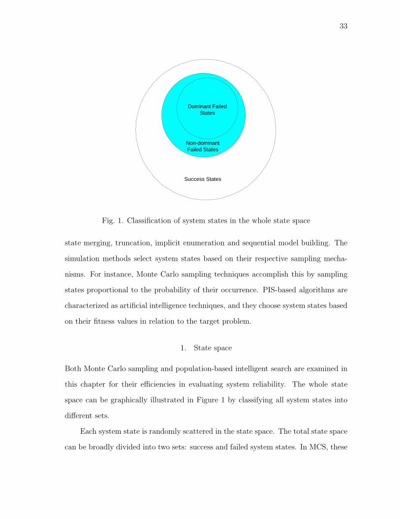
33
Success States
Dominant FailedStates
Non-dominantFailed States
Fig. 1. Classification of system states in the whole state space
state merging, truncation, implicit enumeration and sequential model building. The
simulation methods select system states based on their respective sampling mecha-
nisms. For instance, Monte Carlo sampling techniques accomplish this by sampling
states proportional to the probability of their occurrence. PIS-based algorithms are
characterized as artificial intelligence techniques, and they choose system states based
on their fitness values in relation to the target problem.
1. State space
Both Monte Carlo sampling and population-based intelligent search are examined in
this chapter for their efficiencies in evaluating system reliability. The whole state
space can be graphically illustrated in Figure 1 by classifying all system states into
different sets.
Each system state is randomly scattered in the state space. The total state space
can be broadly divided into two sets: success and failed system states. In MCS, these

34
two sets of system states are sampled proportional to their respective probabilities,
and it is this stochasticity that makes the MCS work. Based on all the samples, the
desired reliability indices are estimated. Even though a state is a repeated sample,
it still counts for index calculation. On the contrary, in PIS, the success states are
meaningless to reliability indices as they do not contribute to these indices. The
painted region shown in Figure 1 includes all the failed system states, which can be
further classified into dominant and non-dominant failed states. As the probability
of non-dominant failed states is relatively low, their impact on reliability indices is
very minor and thus in PIS they are ignored in the calculations. Only the dominant
failed states are meaningful to index calculation in PIS. The major task of MCS and
PIS is to calculate the reliability indices by sampling the search space based on their
respective sampling mechanisms.
2. Monte Carlo Simulation
Monte Carlo simulation methods, which treat the problem as a series of experiments,
estimate reliability indices by simulating the actual process using probability dis-
tributions of state residence times. Non-sequential MCS and sequential MCS are
two typical approaches. In non-sequential MCS, the state space is randomly sampled
regardless of the system operation process chronology. In sequential MCS, the chrono-
logical representation is used, where the system states are sequentially sampled for
certain periods. The duration of the states and the transitions between consecutive
system states are represented in these synthetic sequences. The sequential MCS usu-
ally requires higher computational effort than non-sequential MCS. Some research has
also been done combining analytical methods and simulation methods for power sys-
tem reliability studies [21]–[23]. In this chapter non-sequential simulation or random
sampling is used for comparison with the PIS based methods.

35
a. Computational procedure
Several reliability indices have been proposed in the literature. Perhaps loss of load
probability (LOLP) is the most widely known power system reliability index. This
section gives various steps of Monte Carlo simulation for the LOLP index but the
same process can be used for other indices. Typical steps for LOLP calculation using
simple Monte Carlo simulation can be described as follows.
• Step 1: Select the seed for the random number generator. Set the maximum
iteration number and let the initial iteration number K = 1.
• Step 2: Sample the system state and classify it as loss-of-load or otherwise.
Xi =
1, loss-of-load state;
0, otherwise.(5.6)
Note that the subsequent stopping criteria are not checked until sufficient system
states are sampled and evaluated in order to ensure an unbiased calculation of
these statistical criteria used for halting the program.
• Step 3: Calculate LOLP, variance of the estimated LOLP and the coefficient of
variation.
LOLP =1
K
K∑
i=1
Xi (5.7)
V (LOLP ) =1
K(LOLP − LOLP
2) (5.8)
σ =
√
V (LOLP )
LOLP(5.9)
where K is the total number of samples.
• Step 4: Check whether the coefficient of variation σ is less than a specified
threshold δ . If σ < δ or K > Kmax, stop; otherwise, K = K + 1, go to step 2.

36
b. Stopping criteria
MCS is a fluctuating convergence process [12]. The estimated indices gradually con-
verge to their “real” values as the simulation goes on. MCS should be terminated
when the estimates of reliability indices reach a stipulated degree of confidence. A
stopping criterion is used to provide a compromise between the solution accuracy
and computational effort. As indicated in the above steps, the coefficient of variation
represented in (5.9) is quite often adopted as the convergence criterion, which is a
measure of the uncertainty around the estimates. A number of experiments have
demonstrated that the coefficient of variation for EENS takes the longest time to
stabilize. Thus, when calculating multiple indices, the EENS coefficient of variation
can be used as the stopping rule. Besides the coefficient of variation, the number
of samples can also be used as the stopping criterion. The simulation pauses at a
specified number of samples and the coefficient of variation is checked to see if it is
acceptable. If yes, halt the MCS; or else, increase the number of samples [12].
c. Some remarks
From the steps of the straight Monte Carlo simulation, we can make two observations:
1. For each sampled state, determination needs to be made whether it is a loss of
load state or not. This typically needs a flow calculation to be made. Depending
on the method of flow calculation, this step could impose a significant computational
burden. 2. Due to the random sampling nature, many similar states are sampled in
simulation and their characteristics determined repeatedly. Therefore, the straight
Monte Carlo simulation could be very computationally inefficient.
The main advantages of Monte Carlo simulation include: 1. the ability to model
complex systems in more detail and accuracy than is possible in analytical methods;

37
2. the required number of samples for a given accuracy depends on the variance
which tends to decrease with the system size; 3. the method can not only calculate
the expected value of reliability indices but also their distributions. The primary
disadvantage of Monte Carlo simulation is the lengthy computational time to achieve
satisfactory statistical convergence of reliability index values. The time for conver-
gence is inversely proportional to the loss of load probability.
3. Population-based Intelligent Search
More recently, some methods for intelligent search of state space using PIS algorithms
such as genetic algorithms have been shown to have promise in reliability evaluation
of power systems [13], [24]. Population-based search renders it possible to evaluate
system states in parallel and in this way, a population of individuals is evaluated in
each iteration. Since our problem is not trying to find out a single optimal solution,
this characteristic is of particular benefit in enabling the optimizer to serve as a scan
and classification tool. Distinguished from the random sampling in MCS, in PIS sam-
pling can be interpreted as the “optimization process”. The process of applying PIS
optimization operators in deriving the next generation of individuals is the sampling
mechanism of PIS algorithms. Here the individuals with higher fitness values have
higher chances to be sampled in each iteration. In the problem under consideration,
higher fitness means higher probability of failure.
a. Computational procedure
The general computational flow of any PIS algorithms can be described in the follow-
ing:
• Step 1: A population of individuals is randomly created.

38
• Step 2: Each individual is evaluated based on the specified objective function,
which is used to measure the “fitness” of each individual. Here the term “fitness”
is slightly abused to generally indicate the “goodness” of each individual with
respect to the specific problem, though it is usually used in genetic algorithms.
• Step 3: Determine if any stopping criterion is satisfied. If yes, halt the PIS
algorithm; otherwise, go to next step.
• Step 4: Different PIS operations are applied to each individual in order to create
the next generation of individuals.
• Return to Step 2 until a stopping criterion is satisfied.
b. Stopping criteria
In our problem, PIS is adopted as a scan tool, where a number of meaningful states
are targeted instead of only the optimal or near-optimal one. Different from com-
monly seen optimization problems, here the stopping rule should be set to ensure that
sufficient system states have been identified by the final iteration. Thus, the selection
of stopping criterion may become somewhat trickier. Three stopping criteria may be
used depending on the specific problem. The first one is to halt the algorithm when
the maximum number of iterations is reached. This value is pre-specified and thus
it requires careful tuning. The second stopping rule is the desired number of failure
states. The proper setting of this number requires a very clear insight on the complex
target problem beforehand, which is usually highly difficult or unrealistic to achieve.
The third stopping criterion is to examine the difference between two consecutive ob-
jective values. If the differences keep being below a certain small value for a specified
number of iterations, the algorithm is terminated.

39
c. Some remarks
1. Due to their stochastic search based optimization mechanisms, PIS-based algo-
rithms may become more efficient in handling highly complex and highly nonlinear
large-scale practical systems with respect to other existing methods. 2. The stopping
criteria are somewhat less mathematically strictly defined as compared with MCS,
and in some sense they are more subjective and thus may demand considerable tuning
effort for each specific task.
d. Representative PIS algorithms
Four representative PIS algorithms adopted in this study are briefly introduced here,
which include genetic algorithm (GA), particle swarm optimization (PSO), ant colony
system (ACS), and artificial immune system (AIS). GA is inspired by the biological
evolution with the philosophy of “survival of the fittest” [7]. An individual with
the highest fitness value has the highest chance to be selected to reproduce its next
generation. PSO is invented based on the social behavior of fish schooling and bird
flocking with the philosophy of “following the leader” [8]. The swarm moves as a
group in the search space guided by the best local and global individuals found so
far. ACS is inspired from the collective behavior exhibited in an ant colony on how
to find the shortest route from nest to the food [9]. The trail deposited with the
highest level of pheromone has the highest fitness value. AIS model is built based on
biological immune system by mimicking how the antibodies react to the antigen [11].
The most stimulated antibody has the highest probability to proliferate. All of these
four algorithms are population-based search while featuring different optimization
mechanisms. Due to space restrictions, the detailed discussion of each algorithm is
referred to the respective aforementioned literature.

40
4. Conceptual comparison between MCS and PIS
As indicated previously, the most significant difference between MCS and PIS lies
in their sampling mechanisms. In MCS, system states are sampled based on their
occurrence probability, and both success and failure states sampled contribute to
the estimation of reliability indices. In our scenarios, this means the failure states
have much less probability to be sampled with respect to the success states, since
the failure states have less occurrence probability in power systems. Also, as the
system becomes more reliable, the probability to sample the failure states become
less. This explains why the convergence will be a concern in the reliability assessment
of highly reliable systems. Unlike MCS, PIS is rather problem-dependent, where
system states with higher failure probabilities have higher chances to be selected and
evaluated. Here in PIS the failure probability of system state is used to guide the
search. In some sense, this characteristic enables PIS to have promise to outperform
MCS for some type of problems due to its potentially higher algorithmic efficiency.
The driving force behind each PIS renders the search more purposeful by avoiding
problem-independent random sampling. Also, unlike MCS, in PIS only the failure
states are useful in estimating reliability indices. Due to the difference of estimation
philosophies between MCS and PIS, the deviations of estimation results in relation to
the “real” values may be different between them. For instance, in MCS, the estimated
values of indices may be larger or smaller than the actual values; however, in PIS,
the estimated values are always somewhat smaller than the actual ones. Especially,
in highly reliable systems, since failure states are scattered in the state space in an
extremely sparse fashion, it is possible that the MCS method can not sample the
failure states in their “real” ratio with respect to the total number of system states.
This will inevitably lead to larger estimation errors of the intended reliability indices

41
or even cause convergence problem.
It should be noted that PIS-based algorithms can have a special advantage in
cases where flow calculations using DC/AC load flow are needed to evaluate a sampled
state. When a state is sampled, it can be identified to be loss of load only after the
evaluation process. Since in MCS, majority of the states sampled are success states,
this flow calculation will need be carried out more often. On the other hand, in PIS
the states are sampled in a more directed fashion and thus the evaluation process will
be used more efficiently.
The rigorous analysis of PIS algorithms is difficult [25]. In recent years, some
investigations are being conducted attempting to combine these two methods [26] or
interpret PIS under the well-established MCS framework [27]. Meanwhile, a consid-
erable number of convergence proofs have also been carried out for some PIS-based
algorithms [28].
D. PIS-based Adequacy Evaluation
In PIS algorithms, each individual is regarded as a potential solution and many indi-
viduals comprise a population. For a specific PIS algorithm, individual has different
names. For instance, in GA, each chromosome is an individual, which is made up
of a bunch of genes. In ACS, the tour traveled by each ant (referred to as “ant” for
brevity) is deemed a potential solution. In PSO, each particle flying in the search
space is thought of as a candidate solution. In AIS, each antibody is seen as a po-
tential solution. In this investigation, binary coding scheme is used to represent each
individual, where each bit takes one or zero to indicate the generator state. “One”
and “zero” represent the working and failed status of each generator, respectively.
Since there may be several groups of identical generators used in terms of generator

42
types (conventional or wind turbine generators), generator capacities, and reliability
parameters, all of these generators are grouped accordingly to reduce computational
cost. Assume the generators are divided into n groups, where each group is composed
of states of single or multiple generators and they are represented by binary num-
bers. In this way, multiple binary bits representing an individual are used to indicate
various generation combinations. The target problem is concerned with combinato-
rial optimization, and its objective is to find out the failure state array which can
be used to calculate different adequacy indices. The configuration of each individual
(i.e., system state) can be illustrated as in Figure 2. All the generators involved are
divided into n groups and each bit indicates the corresponding generator condition
(i.e., working or failure status).
C1........CG1 CG1+1........CG2 ........ ........Cmg U1........Umw
G1 G2 GnGn-1........
Fig. 2. Individual (i.e., system-state) representation
There are two major stages in the proposed evaluation procedure: First the
failure-state array with respect to the maximum load demand is derived using PIS, and
then the reliability indices are calculated by convoluting the effective total capacity
with the hourly load based on the state array achieved previously. The evaluation
procedure is extended from that used in [13] by incorporating the variability of wind
power. The computational flow of the proposed evaluation procedure is laid out in
the following.
• Step 1: Generate a population of individuals randomly. The states of both
conventional generators and wind turbine generators (WTGs) are initialized by

43
binary numbers.
• Step 2: Evaluate each individual i based on the defined objective function
(probability of not satisfying load with respect to the maximum load demand
Lmax). If its value is less than the specified threshold (a small value below
which the corresponding states are filtered out), it is assigned a very small
fitness value in order to reduce its chance of participating in subsequent PIS
operations. Based on the attained state array, the overall system probability of
load loss against the maximum load demand is calculated.
The objective value of state i is calculated as follows:
– Calculate the effective generating capacity of state i including WTGs:
Capi,max =
mg∑
j=1
cjgj +mw∑
j=1
ujwr (5.10)
where mg is the number of conventional generators; cj indicates the state
of conventional generator j; gj is the capacity of generator j; mw is the
number of WTGs; uj indicates the state of WTG j, and in each hour pe-
riod, it has only one state: 1 (working) or 0 (failed) for a specific WTG;
wr is the rated power capacity of WTG. Here if the capacity Capi,max is
larger than the maximum load demand Lmax, the fitness of its correspond-
ing individual is assigned a very small value so as to reduce its chance to
contribute to the next generation, since it represents a success state. The
rated WTG capacity is used here in order to ensure that all possible failure
states are included for further evaluations.
– The failure probability of state i can be calculated as follows:
Pi =
m∏
j=1
pj (5.11)

44
where m = mg+mw is the total number of conventional and unconventional
generators, pj can take one of the following two values: for the conventional
units, if cj = 1, then pj = 1 − FORj; and if cj = 0, then pj = FORj.
In a similar manner, for WTGs, if uj = 1, then pj = 1 − FORj; and if
uj = 0, then pj = FORj. FORj represents the forced outage rate (FOR)
of generator j. The probability of each generator down equals its FOR.
Also note that only full outages are considered in this investigation.
– Calculate the number of all possible permutations (i.e., equivalents) of the
evaluated state i:
Copyi =
G1
O1
. . .
Gj
Oj
. . .
Gn
On
(5.12)
where Oj is the number of “ones” in group j of length Gj.
– The fitness of this state is
Fiti = Copyi ∗ Pi (5.13)
It is the objective function to be maximized by the PIS-based optimizer.
Its value (i.e., fitness) is determined by the state of each generator.
– Frequency of this state can be calculated as follows [29], [30]:
Fi = Pi ∗ (m
∑
j=1
(1− bj)µj −m
∑
j=1
bjλj) (5.14)
where bi indicates the generator state; µj and λj are repair rate and failure
rate of generator j, respectively.
– Save information on eligible states including Pi, Fi, and Copyi, which will
be used in subsequent calculations.

45
– Repeat the above procedure for the remaining individuals until all of them
are evaluated. Before each evaluation, the individual under consideration
will be checked to ensure it is not the equivalent of any previously evalu-
ated ones. If it is a previously evaluated state, its fitness will be assigned
a very small number in order to eliminate it very soon in the following
optimization operations.
• Step 3: Increase the iteration number by one;
• Step 4: Check if any stopping criterion is met. If yes, halt the algorithm and
output the state array derived. If no, go to the next step.
• Step 5: Different PIS operators are applied for producing the next generation,
and then repeat the procedure from Step 2 to Step 4 until any stopping criterion
is satisfied.
• Step 6: Calculate the adequacy indices based on the achieved state array. Due to
the time-dependent nature of wind power, the total effective generating capacity
of state i at hour t should be calculated as follows:
Capi,t =
mg∑
j=1
cjgj +mw∑
j=1
ujwj (5.15)
where wj is the actual output of WTG j at hour t. It can be calculated by
wj = αt ∗ wr, where αt is the ratio of WTG output at hour t with respect to
the rated WTG power capacity, and this derating factor is used to calculate the
effective WTG output during hour t. The derating factor is provided or derived
using the wind speed forecasting procedure. It is usually modeled as a random
variable by time series techniques such as the Autoregressive Moving Average
(ARMA) model. In the ARMA model, the power output of WTG in each time

46
step can be represented as a random variable by accounting for its association
with those in previous time steps. The derating factor varies over time, but
for a given time interval, it is realized as a constant value (even though it is
modeled as a stochastic variable) for reliability calculation. Thus, it can be
deemed as a variable “constant”, since it varies along the observation horizon
and meanwhile, it is a fixed value for a given time step. No matter what kind of
method is used to evaluate system reliability, the derating factor of fixed value
in each time period (e.g., hour or smaller time step) is always needed, even if
the derating factor is modeled as a stochastic variable. The time step used for
reliability calculation is determined by the accuracy requirement. If Capi,t is
larger than or equal to the load demand Lt at hour t, it is in fact a success state
and will not be accounted for in calculating reliability indices; Or else, it will
be included in subsequent calculations.
Pft=
sn∑
j=1
Sj ∗ Pj ∗ Copyj (5.16)
where sn is the number of failure states attained previously. Sj is a flag indi-
cating if the loss of load occurs at hour t for state j: it is zero when Capi,t ≥ Lt;
otherwise it is set as one. The value of sn may be smaller than the total number
of states obtained at the first stage, since some of the states may become success
ones at different time periods due to the variations of both loads and derating
factors. Since duration of each time step is one hour, LOLE in hours within the
observation horizon T can be calculated as follows:
LOLE =
NT∑
t=1
Pft(5.17)
The expected energy not supplied (EENS) in megawatts hour can be calculated

47
as follows:
EENS =
NT∑
t=1
PNSt (5.18)
where PNSt is the power not supplied for hour t:
PNSt =sn
∑
j=1
Sj ∗ Pj ∗ Copyj ∗ (Lt − Capj,t). (5.19)
LOLF includes two components: frequency of generating capacity “FG” and
frequency due to load change “FL”.
FG =
NT∑
t=1
LOLFt (5.20)
where LOLFt is the loss of load frequency at hour t:
LOLFt =
sn∑
j=1
Sj ∗ Fj ∗ Copyj; (5.21)
FL =
NT∑
t=2
Vt ∗ [Pft− Pft−1 ] (5.22)
where Vt is zero if the value between brackets is negative, and otherwise it equals
to one.
The LOLF in occurrences during the observation time span T is calculated as
LOLF = FG + FL. (5.23)
Furthermore, based on the state array achieved, the contribution of each system
state to the total system adequacy becomes clear and capacity outage table can be
also built from it. Another major advantage of this approach is that as long as the
actual peak load is not larger than the one used for deriving the state array, the
state array achieved can always be used for calculating the actual adequacy indices
for various scenarios with different peak loads.

48
The proposed procedure can also be used in reliability evaluation of composite
systems, where the transmission failures can be seen as additional component states
besides the generator failures. That is, in PIS, these component states can also be
encoded into an individual in the same way as the generator failures. The objective
function (5.13) indicating the system failure probability can be revised accordingly
by including the transmission failures. In this scenario, power flow analysis is needed
for state evaluation. Similar to the evaluation procedure for generation systems,
here the proposed method can also be divided into two major stages. First, PIS
searches intelligently for failure states through its fitness function, using the linear
programming optimization model to determine if a load curtailment is needed for
each sampled state. Sampled state data are then saved in state array. The sampling
process and evaluation procedure can be linked by the power flow analysis solved
by linear programming. Each time when a system state is sampled, the power flow
analysis routine will be called to determine if a loss of load is caused. After the
search process stops, the second step begins by using all of the saved states data to
calculate the annualized indices for the whole system and at each load bus. Each
power transmission line is assumed to have two states, up and down. Its failure
probability can be calculated from its failure rate and repair rate.
E. Simulations and Evaluation
A WTGs-augmented IEEE Reliability Test System (IEEE RTS-79) is used in simu-
lations [31]. The original RTS has 24 buses (10 generation buses and 17 load buses),
38 lines and 32 conventional generating-units. The system annual peak load is 2850
MW. The total installed generating capacity is 3405 MW. In this study, one uncon-
ventional subsystem comprising of multiple identical WTGs is added to the RTS.

49
Each WTG has an installed capacity of 1 MW, a mean up time of 190 hours and
a mean down time of 10 hours. The hourly derating factors for WTG output can
be found in [15]. These hourly derating factors used in the simulation studies for
reflecting hour-to-hour variations have included the stochastic nature of wind power
and are stochastic variables. Reliability indices are calculated for a time span of one
week and the load cycle for week 51 with peak load 2850 MW, low load 1368 MW
and weekly energy demand 359.3 GWh. Different wind power penetration levels are
examined by incorporating three installed wind power capacities of 100 MW, 200
MW, and 400 MW.
For peak load of 2850 MW with wind power penetration, the system adequacy
indices obtained using the analytical method [15], MCS, and proposed PIS methods
are listed from Table I to Table III. Distinguished from the negative margin method
and clustering method, in the analytical method the mean capacity outage table
is constructed to simultaneously compute EENS, LOLE, and LOLF with reduced
computational cost. The overall system is divided into two subsystems including
the conventional subsystem and the unconventional subsystem (i.e, WTGs). The
computation procedure for these three indices is as follows:
• Build the capacity outage table, the cumulative outage probability and fre-
quency tables for the conventional subsystem, using the unit addition algorithm.
• Build the capacity outage table, the cumulative outage probability and fre-
quency tables for the unconventional subsystem considering the availability of
intermittent sources, in a similar fashion.
• Build the capacity outage table for the overall system through combining ca-
pacity outage tables constructed in the above two steps.

50
• Build the mean capacity outage table for the conventional subsystem based on
the recurrence approach.
• Calculate the hourly contributions to the indices.
• Calculate EENS, LOLE, and LOLF by summation over the whole period of
observation.
The units of LOLE, EENS, and LOLF are h/week, MWh, and occ./week, respec-
tively. The time is in seconds. Here all the four discrete PIS optimizers mentioned
earlier are used to derive the meaningful system states. The population sizes for all
PIS algorithms are set at 300. We can see that the performance of MCS is somehow
the worst among all methods in all scenarios of our problem in terms of solution
quality and computational cost. The solutions derived by all PIS algorithms are
comparable to the ones derived by the analytical method. Among them, the solu-
tions from ACS are slightly more accurate than those of others. GA is the most
computationally expensive one primarily due to its time-consuming genetic opera-
tions. Binary PSO (BPSO) [32] has the shortest convergence time due to its simple
operations. For comparison with another analytical approximation method, a clus-
tering method is used to calculate the EENS [15]. It uses fixed margin increment of
10 MW and clustering with the nearest centroid sorting algorithm. The number of
clusters is set as 80. The EENS’s derived are 207.6943 MWh, 159.1898 MWh, and
98.8874 MWh for integrated wind power capacities of 100 MW, 200 MW, and 400
MW, respectively. We can see that the results obtained from all population-based
intelligent search methods used slightly outperform the clustering method in terms
of EENS accuracy in such settings. Furthermore, as the system complexity increases
(in this context it means more WTGs are integrated), the computational efficiency
advantage of the population-based stochastic search becomes more evident in relation

51
to the analytical method. We can also see that as the power system becomes more
reliable, the effectiveness and efficiency of MCS method are decreased in terms of both
solution quality and computational expense. That is, with more WTGs incorporated,
the solutions become more inaccurate and higher computational costs are caused in
relation to the four PIS-based algorithms. This observation matches the conceptual
analyses presented earlier.
Table I. Reliability indices for unconventional capacity 100 MW
Method LOLE EENS LOLF Time
ACS 1.487890 207.761 0.310570 6.7
AIS 1.487879 207.740 0.310563 6.8
BPSO 1.487856 207.723 0.310559 5.7
GA 1.487820 207.702 0.310543 11.7
MCS 1.493332 208.989 0.311240 19.8
Analytical method 1.487951 207.902 0.310602 8.4
Table II. Reliability indices for unconventional capacity 200 MW
Method LOLE EENS LOLF Time
ACS 1.185620 159.243 0.258272 11.9
AIS 1.185601 159.223 0.258264 12.4
BPSO 1.185583 159.216 0.258256 9.8
GA 1.185560 159.203 0.258251 18.3
MCS 1.174901 157.001 0.256401 34.6
Analytical method 1.185692 159.402 0.258305 16.5
Since more system states are derived as the optimization process proceeds, the
solutions will become more accurate with more iterations. Thus, there should be a

52
Table III. Reliability indices for unconventional capacity 400 MW.
Method LOLE EENS LOLF Time
ACS 0.789780 98.921 0.193233 21.6
AIS 0.789768 98.912 0.193229 22.7
BPSO 0.789760 98.909 0.193221 15.4
GA 0.789740 98.900 0.193213 29.3
MCS 0.771991 96.211 0.190632 59.4
Analytical method 0.789840 99.085 0.193275 29.9
tradeoff between the computational cost and solution accuracy. Here the stopping
criterion set after careful tuning is the number of maximum iterations, which is 100
in this problem. It turns out to be a reasonable number since comparable results are
attained by this generation. Furthermore, as an example, Table IV shows the growth
of reliability indices with the increasing number of iterations by using ACS as the PIS
algorithm in the third evaluation scenario.
Table IV. Growth of reliability indices with the increasing generations
Generations LOLE EENS LOLF
25 0.248773 32.459 0.063098
50 0.503987 70.546 0.138953
75 0.655530 85.999 0.169908
100 0.789780 98.921 0.193233
The size of the entire search space is 2(32+NWTG), where NWTG is the number of
WTGs taking 100, 200, and 400 in our problems. We can appreciate that all three
cases involve a large number of system states. Despite the difference of sampling
mechanisms between MCS and PIS, it is still viable to compare these two methods in

53
terms of number of total samples for deriving the comparable results. In MCS, every
sample counts in index calculation, while in PIS only the sampled failure states are
seen valid. The total samples of MCS in three different evaluation scenarios are around
46,000, 59,000, and 89,000 for deriving the results as shown in the above tables. In
PIS, all calculations are based on the identical total sampling number of 30,000, since
the size of search space is 300×100. Thus, in terms of sampling efficiency, PIS-based
algorithms have exhibited a certain degree of superiority in this problem with respect
to the MCS method, as they are capable of deriving more accurate results with less
number of samples in a shorter time.
Here the commonly used convergence trajectory of PIS is not as illustrative as
that used in optimization problems anymore. For a more informative indication, we
define a ratio to measure the convergence performance (i.e. sampling efficiency) of
different PIS algorithms for the scan and classification task.
λ =Number of meaningful states sampled
Number of total samples(5.24)
This ratio can be used in each generation or across the whole optimization process. It
varies depending on the algorithm efficiency and solution density in the search space.
Table V illustrates the ratios of different PIS-based algorithms in the whole optimiza-
tion process for the first scenario, where 100 WTGs are incorporated. ACS found out
a bit larger number of meaningful states than others, which lead to slightly more ac-
curate results. It should be noted that although this ratio is defined for measuring the
convergence performance of PIS, it also has significance in the context of MCS which
is virtually the estimate of LOLP as defined in (5.7), if the “meaningful states” are
also interpreted as the “dominant failed states”. In this evaluation scenario, the ratio
equals to 0.889%. As compared with PIS, in MCS a smaller proportion of sampled
system states turn out to be dominant failed states. Also, as more WTGs are incor-

54
porated, this ratio will become even smaller because of higher reliability. Further,
in the proposed PIS method, all equivalents of the sampled state are sought out to
avoid repeated sampling and evaluation; however in MCS, due to repeated sampling,
equivalent samples may be evaluated repeatedly. Therefore, as mentioned earlier, in
certain scenarios where flow calculation is required to evaluate each system state, PIS
is promising to outperform MCS further through its directed search.
Table V. Comparison of sampling efficiency of different PIS algorithms in the entire
optimization process.
Method Sampled Meaningful States Ratio λ
ACS 2,041 6.80%
AIS 2,021 6.74%
BPSO 2,016 6.72%
GA 2,002 6.67%
Moreover, the evolution of this ratio in terms of computational iterations is il-
lustrated in Figure 3. Though for each PIS algorithm the trajectories differ with
one another quantitatively, they do exhibit a similar pattern. We can see that as
the optimization proceeds, first this ratio increases gradually because of the fitness-
guided sampling mechanisms of these four PIS-based algorithms. This means that
the proportion of meaningful individuals in the entire population becomes larger as
the optimization proceeds. In particular, the ratio will reach its maximum value
in a certain generation. For instance, in ACS this ratio reaches its maximum in
the 70-th generation, which indicates that in this generation, about 14.4% individ-
uals in the population of size 300 are useful for index calculation. Then, the ratio
after the 70-th generation keeps declining since there are limited dominant states
remaining after previous generations of search, and the search space becomes much

55
sparser. This differs from the traditional convergence trajectory used in optimization
problems, which usually continuously approaches the optimal or sub-optimal value
without such a turning point changing from rising to falling ratios. This is because in
traditional optimization problems, the most recent optimal solution found will not be
worse than its previous one, so its trajectory always keeps moving toward the same
direction (i.e., rising or falling).
10 20 30 40 50 60 70 80 90 1000
0.02
0.04
0.06
0.08
0.1
0.12
0.14
0.16
Iterations
Rat
io λ
GABPSOAISACS
Fig. 3. Ratio of meaningful states and total sampled states
In some scenarios of reliability evaluation, PIS-based algorithms have promise
to exhibit more effective and efficient performance with respect to the exact method
and MCS method. The primary advantages of the proposed PIS method can be
summarized in the following.
• The contribution of each system state to the overall adequacy indices can be
easily calculated and identified. This feature is important when a sensitivity

56
study is desired to determine system states which have the most significant
impact on the overall system reliability.
• The state array derived by the evaluation procedure may be reused for different
load levels. As long as the actual peak load is smaller than the peak load used to
derive the state array, the state array can be used to calculate reliability indices
for different load demands. Moreover, the second-stage evaluation procedure
can be generically used to calculate reliability indices for any set of failure
states provided.
• In Monte Carlo simulations, system states are sampled dependent on their prob-
abilities without consideration of their relevance to the problem being solved.
However, in intelligent search methods, the system states most relevant to the
target problem have higher chances to be sampled due to their higher fitness
values, regardless of their occurrence probabilities. This fitness-guided search
characteristic may be beneficial in adequacy assessment since it enables the
search to avoid evaluating irrelevant system states, which do not contribute or
contribute very trivially to the overall reliability indices. As a result, in some
scenarios the time used for adequacy evaluation can be reduced and therefore
the algorithmic efficiency is improved.
• The computational time is not considerably affected by the system reliabil-
ity characteristics. In Monte Carlo simulations, longer computational time is
needed to achieve simulation convergence with higher system reliability, and it
is possible that larger approximation errors and sluggish convergence perfor-
mance may be caused. In highly reliable systems, PIS exhibits more robust
behavior than MCS due to their different sampling mechanisms.

57
• The computational time is reduced in evaluating scenarios where a large number
of power sources with relatively small capacities are involved. For methods
which need the construction of capacity outage table, it takes more time to build
the outage table by incorporating the state of each WTG, which, however, has
no significant impact on the entire system reliability if only one unit outage is
considered each time. The optimization mechanism of PIS makes system states
related to these small capacity additions die off or reproduce very fast and thus
considerably reduces the computation expense required.
• The method can be generally used in adequacy evaluation of power-generating
systems with and without time-dependent sources. Furthermore, it has no
inherent limitations in dealing with larger-sized systems based on its conver-
gence mechanism. This is in actuality one salient merit of this population-
based stochastic search approach. On the contrary, most analytical methods
become much less efficient or even unable to resolve the problem as the system
complexity and size increase.
• The parallel or distributed computation can be accomplished simply using par-
titioning based on the probabilities or load demands [13]. This can considerably
increase the computational efficiency of different PIS-based algorithms.
• Although the comparison between MCS and PIS in this chapter is based on
generating systems, most of the understanding and insights presented are ap-
plicable to power system reliability in general, e.g., multi-area and composite
system reliability analysis.

58
F. Summary
Due to the penetration of time-dependent sources such as wind turbine generators,
it becomes more complicated to evaluate the adequacy of power-generating systems
which themselves have uncertainties such as equipment failures. In this chapter, we
adopted a two-stage procedure to evaluate the system adequacy. First a set of dom-
inant failure states is derived by a specific PIS algorithm based on its convergence
mechanism. Then, three major reliability indices are calculated based on these fail-
ure states by also considering the intermittency of wind power. A numerical study
is carried out to demonstrate the usefulness of the proposed method. As we can see,
the effectiveness of the proposed evaluation procedure is largely determined by the
efficiency of the search algorithm. PIS-based optimizers enable the search to avoid
less meaningful system states and seek out the most significant states efficiently. Also
some comparative studies are carried out conceptually and numerically in relation
to the Monte Carlo simulation method. PIS has shown to be effective in searching
out eligible system states within a reasonable time. The advantages of the proposed
method are also evaluated with respect to other existing methods including the ana-
lytical method and Monte Carlo simulation. Our future work includes incorporating
other system uncertainties such as stochastic generation/load variations as well as
improving PIS-based algorithms in handling the target problem.

59
CHAPTER VI
RELIABILITY-CONSTRAINED OPTIMUM PLACEMENT OF RECLOSERS
AND DISTRIBUTED GENERATORS IN DISTRIBUTION NETWORKS USING
ANT COLONY SYSTEM ALGORITHM
Optimal placement of protection devices and distributed generators (DGs) in radial
feeders is important to ensure power system reliability. Distributed generation is
being adopted in distribution networks with reliability enhancement as one of the
objectives. In this chapter, an ant colony system (ACS) algorithm is used to derive
the optimal recloser and DG placement scheme for radial distribution networks. A
composite reliability index is used as the objective function in the optimization pro-
cedure. Simulations are carried out based on two practical distribution systems to
validate the effectiveness of the proposed method. Furthermore, comparative studies
in relation to genetic algorithm are also conducted.
A. Introduction
As said earlier, one of the objectives of incorporating distributed generation (DG) in
the distribution networks is reliability enhancement [5], [33]–[36]. In a DG-enhanced
feeder, power flow is not unidirectional and conventional protection logic needs to
be modified accordingly. A faulted branch can be energized from both ends and the
protection devices are desired to interrupt the fault current. There are primarily three
scenarios [37] in the optimal design of a DG-enhanced distribution system:
• Optimal recloser placement for a given DG allocation;
• Optimal DG placement for a given recloser placement;
• Optimal recloser and DG placement.

60
In essence, such problems are highly combinatorial and the corresponding objec-
tive functions are usually nondifferentiable. Thus, traditional analytical approaches
such as linear and nonlinear programming have difficulty in dealing with these prob-
lems. More recently, various computational intelligence techniques have been de-
veloped to find the optimum or near-optimum solutions based on guided stochastic
search. Among them, swarm intelligence is a relatively novel technique which can be
used for complex engineering design optimization [38], [39]. Especially, ant colony
search based algorithms are a kind of outstanding discrete optimizers [40]–[45]. In
this study, an ant colony system (ACS) algorithm is proposed to optimize the recloser
(or DG) placement for a fixed DG (or recloser) allocation. The idea can be extended
to the simultaneous placement of both reclosers and DGs.
The remainder of the chapter is organized as follows: In Section B, the problem
is formulated, where the optimum replacement of reclosers and DGs in distribution
networks is introduced and a composite reliability index is defined. The inner working
of the ant colony search algorithm and its basic steps are discussed in Section C.
In Section D, the proposed method for optimal recloser and DG placement in two
practical distribution systems is detailed. Simulation results and analysis are given
in Section E. Finally, conclusions are drawn and future research is suggested.
B. Problem Formulation
A DG-enhanced radial feeder is shown in Figure 4 [37]. It includes four reclosers
and two generators. If there are no generators in the distribution network, the first
recloser upstream the fault will operate in the presence of a fault anywhere on the line.
This will make the customers located downstream the recloser lose service. When the
distributed generators are incorporated, service can still be provided to some islands

61
with DG. For instance, if a fault occurs between recloser 1 and recloser 2 during
system operations, only recloser 1 will operate if there is no DG in the feeder. Thus,
loss of service will be caused to the customers downstream this recloser. However, if
there are DGs incorporated as shown in the figure, both recloser 1 and recloser 2 will
operate and thus an island is formed. The distributed generators may still be capable
of providing satisfactory service to the islanded zone.
DGLateral
DG
Recloser 1 Recloser 2 Recloser 3 Recloser 4
Fig. 4. Distributed generation-enhanced radial feeder
In the DG-enhanced distribution network, the sequence of events after a fault
occurs is as follows: First DG is tripped, and the fault is detected and isolated by
one or more protection devices, then the DG reconnects if it is not within the faulted
zone. After the fault is cleared, recloser synchronizes its reclosing operation with the
DG. As we can see, the locations of protection devices and distributed generators are
highly dependent. Properly placed reclosers and distributed generators are crucial to
achieve the optimal design of a DG-enhanced distribution network in terms of system
reliability and investment costs.
The objective of protection devices and DGs placement in a radial feeder is to
maximize the distribution network reliability under certain constraints. The system
average interruption duration index (SAIDI) and the system average interruption
frequency index (SAIFI) are typically used to measure the average accumulated du-
ration and frequency of sustained interruptions per customer [37]. They are defined

62
as follows:
SAIDI =
∑
uiNi∑
Ni
(6.1)
where Ni is the number of customers of load point i, and ui is the outage time.
SAIFI =
∑
riNi∑
Ni
(6.2)
where ri is the failure rate.
For the purpose of optimization, we define a composite reliability index through
weighted aggregation of these two indices:
C = WSAIFI ∗SAIFI
SAIFIT
+ WSAIDI ∗SAIDI
SAIDIT
(6.3)
where Wx indicates the weight for the corresponding reliability index, and the sub-
script T indicates the target value. This composite reliability index accounts for
both SAIDI and SAIFI, which are the two most widely used indices for measuring
the distribution system reliability. In this formulation, we incorporate the desired
values of both indices which are empirically justified. The optimization algorithm is
used to minimize the weighted composite index including interruption duration and
frequency components. The smaller the value of the defined reliability index (i.e., ob-
jective function) is, the higher the system reliability becomes. The design constraints
here are the number of reclosers or DGs available for this purpose coupled with the
number of candidate locations determined by the system configuration.
C. Ant Colony System Algorithms
This section describes the basic inner working as well as the basic steps in a typical
ant colony system algorithm.

63
1. Basic principle
Ant colony algorithms are based on the behavior of social insects with an exceptional
ability to find the shortest paths from the nest to the food sources using a chemical
substance called pheromone [9]. Pheromone is used by the ants to communicate
information with one another regarding the search path and to judge where to go.
Ants deposit a certain amount of pheromone while walking, and each ant prefers
to follow a direction rich in pheromone rather than a poorer one in a probabilistic
fashion. Ant colony system (ACS) used in this study is extended from ant colony
optimization (ACO), and it has a better performance than ACO in most engineering
application scenarios. In ACS, the term “tour” is very often used to illustrate its
mechanism. Each tour is a potential solution and it can be interpreted differently
according to the nature of specific problems. For instance, in Traveling Salesman
Problems (TSPs), it indicates a route connecting different cities, and in our problem,
it represents a solution of recloser or DG locations.
2. Basic steps
The basic steps in the ant colony system (ACS) algorithm can be summarized as
follows:
• Step 1: Initialization: In this phase, all ants are positioned on randomly gener-
ated starting nodes and initial values for trail intensity are set for each edge.
• Step 2: Tour construction: In this phase, each ant chooses the next node to
move, considering the trail intensity and distance. Ants prefer to move to states
which are connected by shorter edges or with higher pheromone intensity. This
process is repeated until all ants finish their tours.
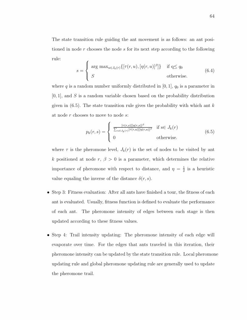
64
The state transition rule guiding the ant movement is as follows: an ant posi-
tioned in node r chooses the node s for its next step according to the following
rule:
s =
arg maxu∈Jk(r)[τ(r, u), [η(r, u)]β] if q≤ q0
S otherwise.(6.4)
where q is a random number uniformly distributed in [0, 1], q0 is a parameter in
[0, 1], and S is a random variable chosen based on the probability distribution
given in (6.5). The state transition rule gives the probability with which ant k
at node r chooses to move to node s:
pk(r, s) =
[τ(r,s)][η(r,s)]β∑
u∈Jk(r)[τ(r,u)][η(r,u)]βif s∈ Jk(r)
0 otherwise.(6.5)
where τ is the pheromone level, Jk(r) is the set of nodes to be visited by ant
k positioned at node r, β > 0 is a parameter, which determines the relative
importance of pheromone with respect to distance, and η = 1δ
is a heuristic
value equaling the inverse of the distance δ(r, s).
• Step 3: Fitness evaluation: After all ants have finished a tour, the fitness of each
ant is evaluated. Usually, fitness function is defined to evaluate the performance
of each ant. The pheromone intensity of edges between each stage is then
updated according to these fitness values.
• Step 4: Trail intensity updating: The pheromone intensity of each edge will
evaporate over time. For the edges that ants traveled in this iteration, their
pheromone intensity can be updated by the state transition rule. Local pheromone
updating rule and global pheromone updating rule are generally used to update
the pheromone trail.

65
– Local updating rule: In deriving a solution, ants visit edges and alter their
pheromone level based on the local updating rule:
τ(r, s)←− (1− ρ)τ(r, s) + ρτ0 (6.6)
where 0 < ρ < 1 is a heuristically defined coefficient, and τ0 is the initial
pheromone level.
– Global updating rule: Global updating is carried out in the best tour
found so far after all ants have finished their tours. The pheromone level
is updated using the global updating rule:
τ(r, s)←− (1− α)τ(r, s) + α∆τ(r, s) (6.7)
where
∆τ(r, s) =
(Lgb)−1 if (r,s)∈ Global-best-tour
0 otherwise.(6.8)
where 0 < α < 1 is the pheromone decay parameter, and Lgb is the length
of the globally best tour.
• Stopping criteria: The above optimization process is terminated if the tour
counter reaches the maximum prespecified number of iterations or all ants
choose the same tour.
D. The Proposed Approach
In this study, two designs will be investigated: recloser placement for fixed DG loca-
tions and DG placement for fixed recloser locations. In this section, recloser placement
will be used to illustrate the proposed method, which can also be applied to the op-
timum DG placement design in a similar fashion. In the DG-enhanced distribution

66
network, optimization becomes more complicated as compared with the traditional
one. Quite often, it is difficult to locate the optimal recloser positions for support-
ing the normal power supply of isolated islands in the presence of faults. In this
investigation, we propose an ant colony system algorithm to seek out the optimal re-
closer locations by minimizing the aforementioned composite reliability index. Since
reclosers can only be placed on the feeder branches, this problem is concerned with
discrete optimization. It appears natural to think of the ant colony system algorithm
for this application considering its ability to handle discrete optimization problems.
1. Search space
In the optimal recloser placement problem, the elements of the potential solution are
positions of individual reclosers to be placed on the feeder. Figure 5 shows the search
space of the recloser placement problem, where N is the number of available reclosers
and M is the number of possible branches where reclosers may be placed. All possible
candidate locations for recloser n are represented by the states in the search space
corresponding to stage n. The number of stages equals to the number of reclosers.
Each ant starts its tour at the home colony and stops at the destination. The ant
opts for the state to move toward with a certain probability, which is a function of the
amount of pheromone deposited on the connecting edges of each state. When an ant
travels from one stage to the next, the state of each stage is recorded in the location
list. In order to enable the ant to choose legal tours, transitions to the locations
that have been occupied are prohibited until a tour is completed. After a tour is
accomplished, the location list of each ant is used to calculate its current solution,
i.e., the value of the objective function.

67
Destination
Nest
. . . . . .
. . . . . .
. . . . . .
. . . . . .
Stage
1
2
N-1
N
State
Number of candidate locations
Number of reclosers
1 2
. . . . . .
M-1 M
.
.
.
.
.
.
.
.
.
.
.
.
Fig. 5. Search space of the problem
2. Reliability evaluation
The procedure for calculating the system reliability is illustrated in Figure 6. For
each recloser configuration (i.e., a potential solution), a composite reliability index
is derived by determining the reliability zones that are bounded by the reclosers,
simulating the faults in those zones, determining the online and offline loads, and
finally calculating the value of the composite reliability index. For each reliability
zone with DG, the maximum active power output of all generators in this zone is
calculated after a fault occurs in other zones. The value is then compared with
the load duration curve of this zone load. The number of faults is reduced by the

68
percentage of time that the zone generation is larger than the zone load.
3. Solution construction and pheromone updating
Each ant updates the pheromone trails after it builds up a solution. Thus, ants
can use different pheromone intensities to construct solutions in order to achieve
diversification of solutions. On the other hand, the global updating is performed
after all ants construct solutions by further adjusting the pheromone level of the best
path achieved so far.
• Solution construction: Let τxyij be the pheromone intensity of trail on edge (i, j)
between the consecutive stages x and y at iteration t. Each ant at state i of
stage x opts for the next stage based on the state transition rules. For q > q0,
the transition rules are defined in the following:
pxyij (t) =
[τxyij (t)][ηxy
ij ]β∑
j∈stagey[τxyij (t)][ηxy
ij ]β(6.9)
For q ≤ q0, the following state is selected:
arg maxj∈stagey[τxyij (t)][ηxy
ij ]β (6.10)
where ηxyij is the reduction of reliability index C values between stage x and y.
β is the parameter that controls the relative importance of trail intensity versus
the C reduction between the consecutive stages.
• Pheromone updating: After the solution is constructed, ant i has its location
list Ω(t)i and fitness evaluation C(Ω
(t)i ). All trail intensity can be updated based
on the evaporation formula for local update:
τxyij (t + 1) = ρ× τxy
ij (t) + τxy,(0)ij (6.11)

69
where τxy,(0)ij is a small positive value. The ant with the highest fitness at
each iteration will deposit the largest amount of pheromone to the edges of its
location list. If ant k has the best solution in this tour, then the pheromone
intensity of these edges in its location list can be further revised by the global
updating rule
τxyij (t + 1) = τxy
ij (t + 1) +Kpher
C(Ω(t)k )
, x, y ∈ Ω(t)k (6.12)
where Kpher is a constant relevant to the trail deposit. It can be appreciated
that the smaller the value of the reliability index is, the larger the additional
pheromone deposit will be.
4. Computational procedure
The computational procedure of the proposed optimization algorithm is shown in
Figure 7, which is detailed in the following:
• Ant production initialization: The initial ant positions and the initial pheromone
levels are created. Number of available reclosers and the capacity of each dis-
tributed generator are specified. The configuration of the radial feeder is rep-
resented to indicate all the candidate device locations.
• Fitness evaluation: The fitness of all ants is evaluated in terms of the objective
function defined in (6.3). That is, the fitness value of each recloser placement
scenario is assessed according to its resultant system reliability. With the eval-
uated fitness of all ants, the pheromone can be added to the particular direction
that the ants have chosen.
• Ant dispatch: The ants are dispatched based on the level of pheromone and
distance. As shown in (6.9) and (6.10), each ant chooses the next state to move

70
considering τij and ηij values. If an ant k positioned in state i chooses the next
state j to move, then such a movement can be represented as follows:
– If q > q0, select the next state randomly with the probability represented
by (6.9):
– If q ≤ q0, select the next state with the best local pheromone-distance
profile as indicated in (6.10).
Let K be the number of ants, then for each iteration, these K ants perform K
movements during interval (t, t + 1). The pheromone of the visited path can be
dynamically adjusted by (6.11). After all ants have completed their tours, the
shortest path found by the ants is allowed to update its pheromone based on
(6.12), which corresponds to the best recloser configuration found thus far.
• Termination conditions: The optimization process does not halt until the num-
ber of iterations reaches the pre-specified value, or the value of the objective
function ceases improving for a certain number of iterations. The best path
chosen among all iterations is the desired recloser placement scheme, i.e., the
optimal solution to our problem.
E. Simulation Results and Analysis
As mentioned earlier, two design cases will be investigated in the simulation studies.
First, the proposed method is tested on a 69-segment, 8-lateral distribution feeder as
shown in Figure 8 [37]. We assume that DG locations are fixed in the distribution
system and all reclosers function identically. There are eight laterals, six of which are
connected to a single DG at their ends. System parameters used in the simulations
can be found in [46]. It is obvious that the enumeration method is not efficient, if

71
not impossible, for such a system. Here we assume that the fault incidence rate and
the duration of faults are uniform over all feeder branches. Also, in the presence of a
fault, only the minimum number of reclosers close to the fault are activated in order
to isolate the fault. The total nominal feeder load is 3.8 MW. The reliability index
weights are chosen as follows: WSAIFI = 0.33, and WSAIDI = 0.67. The target values
of the reliability indices are set as follows: SAIFIT = 1.0, and SAIDIT = 2.2. They
are empirically justified and indicate the satisfactory level of reliability.
The simulation program was coded using Visual C++ 6.0 and run in a 2.20 GHz
Pentium-IV personal computer. Many parameters can impact the performance of the
ACS algorithm. β reflects the relative importance of the reduction of objective func-
tion values between consecutive stages with respect to the trail intensity. ρ represents
the trail persistence and (1 − ρ) is the trail pheromone evaporation rate. Kpher is a
large constant associated with the quantity of trail deposit. The proper tuning of
ACS parameters is crucial to achieve an effective optimizer. After careful tuning, we
selected the following parameter values: number of ants = 200, number of iterations
= 200, β = 1.0, ρ = 0.73, and Kpher = 60, 000. The update rule specified in (6.11)
and (6.12) may cause the early stagnation during the stochastic search. In this situa-
tion, the trails on certain edges are so high that the ants will deposit more and more
phoromone in this trail. This is undesirable since this kind of premature convergence
usually leads to the local optimum. To avoid search stagnation, the allowed range of
the pheromone trail intensity is specified as follows:
γ(r, s) =
τmin if γ(r, s) ≤ τmin
τmax if γ(r, s) ≥ τmax.(6.13)

72
In this study, the upper and lower bounds are chosen as follows:
τmax =1
Cgbest
(6.14)
where Cgbest is the global best solution achieved so far, and
τmin =τmax
K2(6.15)
where K is the number of ants. As we can see, in Max-Min ACS, upper and lower
bounds are added to impose explicit limits on pheromone trails during the optimiza-
tion process. The bounds are selected based on empirical observations in some initial
experiments, and during optimization they keep changing based on the global best so-
lution obtained so far. This Max-Min ACS algorithm is capable of achieving a higher
degree of exploration by trying more alternatives. The simulation results obtained
based on different DG capacities and different numbers of reclosers are listed from
Table VI to Table IX.
Table VI. No distributed generators in the distribution system (test system 1)
Number of reclosers Reliability index value Recloser locations
1 3.9560 8-9
2 2.8695 8-9, 30-31
3 1.9012 3-4, 30-31, 47-48
4 1.6042 3-4, 27e-28e
30-31, 47-48
5 0.9033 3-4, 11-12, 30-31,
47-48, 28e-65
Generally speaking, from the simulation results obtained, we can see that for a
given capacity of distributed generators, the system reliability increases with more

73
Table VII. Maximum power of each distributed generator = 0.3 MW (test system 1)
Number of reclosers Reliability index value Recloser locations
1 3.8671 8-9
2 2.7005 8-9, 27-28
3 1.8109 3-4, 30-31, 47-48
4 1.3237 3-4, 27e-28e,
30-31, 47-48
5 0.8001 3-4, 10-11, 27e-28e,
30-31, 47-48
reclosers used. For the same number of reclosers used, the higher the maximum
output of distributed generators, the higher the system reliability will become. When
there is only one recloser, its optimal location complies with the traditional device
placement rule, that is, the recloser should be put as near as possible to the central
part of the entire radial feeder. Especially, provided that the loads are uniformly
distributed, 25% reliability improvement can be achieved [37]. For the cases of the
feeder with more reclosers, some branches turned out to be particularly important in
improving the system reliability. For instance, in some cases, the branch between bus
47 and bus 48 is a crucial location for protective device placement since the addition
of recloser in this position will considerably increase the system reliability. From the
simulation results, we can see that the appropriate selection of DG capacity as well
as the proper placement of protective devices are both very important in ensuring the
system reliability.
For comparison purpose, genetic algorithm (GA) is also used to derive solutions
for this problem, which has turned out to be very effective in various engineering
optimization applications [7]. In GA, each candidate solution is deemed a chromosome

74
Table VIII. Maximum power of each distributed generator = 0.5 MW (test system 1)
Number of reclosers Reliability index value Recloser locations
1 3.5022 8-9
2 2.3341 8-9, 28-29
3 1.7432 8-9, 27-28, 50-51
4 1.1987 3-4, 30-31,
47-48, 66-67
5 0.7100 4-5, 10-11, 30-31,
47-48, 67-68
and the stochastic search is carried out based on a population of chromosomes. The
defined composite reliability index is to be minimized and its value is seen as an
indication of fitness for each chromosome. The higher the fitness value is, the higher
the chromosome’s chance to survive becomes. The computational procedure of GA
for handling the target problem primarily includes the following steps:
• Step 1: Initially a set of chromosomes is created in a random fashion;
• Step 2: The fitness of each chromosome is evaluated based on the objective
function defined;
• Step 3: Based on the fitness value of each chromosome, different genetic oper-
ators including reproduction, crossover, and mutation are applied in the entire
population in order to produce the next generation of chromosomes.
• Step 4: Repeat Step 2 and Step 3 until any stopping criterion is satisfied. The
chromosome with the highest fitness value is the final solution to the target
problem.

75
Table IX. Maximum power of each distributed generator = 1.0 MW (test system 1)
Number of reclosers Reliability index value Recloser locations
1 3.3012 8-9
2 2.1455 8-9, 49-50
3 1.5066 4-5, 27e-28e, 47-48
4 1.0340 8-9, 28-29,
36-37, 49-50
5 0.5988 3-4, 10-11, 30-31,
49-50, 67-68
The simulation program was also coded in Visual C++ 6.0 and run in the same
personal computer. In the simulations, the population size is 200, crossover rate is
0.65, and mutation rate is 0.05. Elitist strategy is used to preserve the best solutions
found in each iteration, and the elite count is 2. The maximum number of iterations
is 200, which is used as the stopping criterion.
The design scenarios where GA and ACS have different results are listed in Table
X, and the different results are shown in Table XI.
As we can see from Table XI, the proposed ACS method outperforms the GA
method in terms of solution quality, since in these design scenarios better locations
are found for achieving higher system reliability by the proposed method. Further-
more, the computational time of ACS for deriving the solutions is about 14.4 seconds
in different design scenarios, while that of GA is around 27.3 seconds. Thus, its
computational efficiency is significantly higher than that of GA.
It should be noted that there are still some limitations which may lower the
efficiency of the proposed method. For instance, ACS has some dependency on initial
points, and the most effective combination of different parameters requires some time

76
Table X. Design scenarios where GA and ACS have different results (test system 1)
Design scenarios DG capacity (MW) Number of reclosers
DS 1 0.3 2
DS 2 0.5 3
DS 3 0.5 4
DS 4 0.5 5
DS 5 1 2
DS 6 1 3
DS 7 1 4
to tune. Also its final outputs have some stochastic characteristic. However, there are
no inherent limitations for our proposed method to deal with larger-sized problems
due to its guided stochastic search characteristic. It may take a longer time for the
ACS to converge because more potential solutions are to be evaluated. But the extra
time needed is not as significant as that in analytical methods, since its computational
efficiency is relatively insensitive to system complexity and size. In actuality, with
respect to analytical methods, one salient merit of the proposed method is its ability
to deal with large-sized systems due to its outstanding convergence mechanism. Most
analytical methods become much less efficient or even unable to resolve the problem
when the system complexity and size increase.
Next, the design case of DG placement in fixed recloser locations is examined.
The computational procedure is the same as presented in Section IV, except that here
the DGs are to be placed. A larger-sized distribution system is used to demonstrate
the effectiveness of the proposed method. The actual 394-bus and 1123-node radial
distribution network [47] consists of 199 loads, 104 laterals/sub-laterals, and 44 nor-
mally closed reclosers. The total nominal load is 28.2 MW. Its one-line diagram is

77
Table XI. Comparison of different results obtained from GA and ACS (test system 1)
Scenarios Schemes Reliability value Recloser locations
DS 1 GA 2.7407 8-9, 30-31
ACS 2.7005 8-9, 27-28
DS 2 GA 1.7750 8-9, 28-29, 51-52
ACS 1.7432 8-9, 27-28, 50-51
DS 3 GA 1.2089 4-5, 30-31, 47-48, 67-68
ACS 1.1987 3-4, 30-31, 47-48, 66-67
DS 4 GA 0.7156 3-4, 10-11, 30-31, 47-48, 66-67
ACS 0.7100 4-5, 10-11, 30-31, 47-48, 67-68
DS 5 GA 2.1698 8-9, 27-28
ACS 2.1455 8-9, 49-50
DS 6 GA 1.5165 3-4, 28e-65, 47-48
ACS 1.5066 4-5, 27e-28e, 47-48
DS 7 GA 1.0384 8-9, 27-28, 36-37, 48-49
ACS 1.0340 8-9, 28-29, 36-37, 49-50
shown in Figure 9. Note that in this study each DG will be connected to a single
bus, and the design objective is to connect DGs to the appropriate buses to enhance
the overall system reliability. The reliability index weights are chosen as those in
the first design, and the target values of the reliability indices are set as follows:
SAIFIT = 1.2, and SAIDIT = 2.7. The results derived by the proposed method are
listed from Table XII to Table XIV for different design scenarios. For comparison,
GA is also used to place the DGs. The design scenarios where GA and ACS have
different results are listed in Table XV, and the different results are shown in Table
XVI.

78
Table XII. Maximum power of each distributed generator = 0.3 MW (test system 2)
Number of DGs Reliability index value DG locations
1 1.1976 157
2 1.1345 127, 157
3 1.0788 30, 127, 157
4 1.0464 30, 127, 157, 312
5 1.0207 30, 127, 157, 312, 336
Table XIII. Maximum power of each distributed generator = 0.5 MW (test system 2)
Number of DGs Reliability index value DG locations
1 1.1644 157
2 1.0907 70, 157
3 1.0245 70, 127, 157
4 0.9722 17, 70, 127, 157
5 0.9301 17, 70, 127, 157, 312
As we can see from Table XI, the proposed ACS method outperforms the GA
method in terms of solution quality, since in these design scenarios better locations
have been found which are capable of achieving higher system reliability. Further-
more, the computational time of ACS for deriving the solutions is about 43.7 seconds
in different design scenarios, while that of GA is around 90.6 seconds. Thus, its
computational efficiency is significantly higher than that of GA.
F. Summary
Distributed generation is being introduced into the traditional distribution network
in order to enhance the power system reliability. The optimal placement of protection

79
Table XIV. Maximum power of each distributed generator = 0.7 MW (test system 2)
Number of DGs Reliability index value DG locations
1 1.1327 157
2 1.0521 70, 157
3 0.9850 70, 157, 336
4 0.9234 70, 157, 227, 336
5 0.8726 17, 70, 157, 227, 312
devices and DGs is crucial for achieving such an objective. In this chapter, an opti-
mization procedure based on the ant colony system algorithm is developed to seek out
the optimal recloser and DG locations by minimizing a composite reliability index.
The simulation results from two test distribution systems validate the effectiveness
of the proposed method. Furthermore, comparative studies with respect to genetic
algorithm are also carried out. In future research, we will investigate the simultaneous
placement of both reclosers and distributed generators, which are dependent on one
another. More comprehensive reliability indices may be defined to guide the search
process, and adaptive and automatic tuning can be introduced to further improve
ACS efficiency. Also, the operational costs may be incorporated by minimizing the
customer interruption costs.

80
Table XV. Design scenarios where GA and ACS have different results (test system 2)
Design scenarios DG capacity (MW) Number of DGs
DS 1 0.3 2
DS 2 0.7 2
DS 3 0.5 3
DS 4 0.7 3
DS 5 0.3 4
DS 6 0.7 4
DS 7 0.3 5
DS 8 0.5 5
DS 9 0.7 5

81
Recloser placement
Determination ofreliability zones
Fault simulations
Comparison of islandload demand with thegeneration available
Calculation of thecomposite index
Next iteration
The first ant
All the ants have beenevaluated?
No
Yes
Fig. 6. Flow chart for calculating system reliability of each recloser configuration

82
Start
Initialization of search space anddetermination of ACS parameters
Set the iteration number as zero
Dispatch each ant based on the probabilityof each edge and update location list
Compute the composite reliability indexaccording to (6.3)
Update the trail pheromone intensity ofeach ant based on (6.11)
Increase the iteration number
Satisfy any termination criteria?
End
No
Yes
Find the best solution of this iteration
Further revise the trail pheromone intensityof the best solution based on (6.12)
Fig. 7. Computational procedure for the proposed algorithm.

83
G
DG
DG
DG
DG
DG
DG
35
36
37
38
55
56
57
58
012
345
6
7
8
9
10
11
12
13
14
15
16
17
18
19
20
21
22
23
24
25
26
40
41
42
43
44
45
46
47
48
49
50
51
52
53
54
27
28
29
30
31
32
33
34
27e
28e
65
66
67
68
69
70
88
89
90
Fig. 8. One-line diagram of the 69-bus test distribution system

84
Fig. 9. One-line diagram of the 394-bus test distribution system [47]

85
Table XVI. Comparison of different results obtained from GA and ACS (test system
2)
Scenarios Schemes Reliability value DG locations
DS 1 GA 1.1466 157, 193
ACS 1.1345 127, 157
DS 2 GA 1.0589 157, 193
ACS 1.0521 70, 157
DS 3 GA 1.0468 70, 157, 193
ACS 1.0245 70, 127, 157
DS 4 GA 1.0029 127, 193, 336
ACS 0.9850 70, 157, 336
DS 5 GA 1.0572 127, 193, 227, 360
ACS 1.0464 30, 127, 157, 312
DS 6 GA 0.9421 70, 193, 227, 312
ACS 0.9234 70, 157, 227, 336
DS 7 GA 1.0426 127, 157, 282, 312, 336
ACS 1.0207 30, 127, 157, 312, 336
DS 8 GA 1.0106 70, 127, 157, 282, 312
ACS 0.9301 17, 70, 127, 157, 312
DS 9 GA 0.9033 70, 157, 227, 282, 312
ACS 0.8726 17, 70, 157, 227, 312

86
CHAPTER VII
RISK AND COST TRADEOFF IN ECONOMIC DISPATCH INCLUDING WIND
POWER PENETRATION BASED ON MULTI-OBJECTIVE MEMETIC
PARTICLE SWARM OPTIMIZATION∗
Utilization of renewable energy resources such as wind energy for electric power gen-
eration has assumed great significance in recent years. Wind power is a source of
clean energy and is able to spur the reductions of both consumption of depleting fuel
reserves and emissions of pollutants. However, since the availability of wind power is
highly dependent on the weather conditions, the penetration of wind power into tra-
ditional utility grids may incur certain security implications. Therefore, in economic
power dispatch including wind power penetration, a reasonable tradeoff between sys-
tem risk and operational cost is desired. In this chapter, a bi-objective economic
dispatch problem considering wind penetration is first formulated, which treats op-
erational costs and security impacts as conflicting objectives. Different fuzzy mem-
bership functions are used to reflect the dispatcher’s attitude toward the wind power
penetration. A multi-objective memetic particle swarm optimization (MOMPSO)
algorithm is adopted to develop a power dispatch scheme which is able to achieve
compromise between economic and security requirements. Numerical simulations in-
cluding comparative studies are reported based on a typical IEEE test power system
to show the validity and applicability of the proposed approach.
∗Parts of this chapter are reprinted from Electric Power Systems Research, Vol.78, No. 8, L. Wang and C. Singh, Balancing risk and cost in fuzzy economic dispatchincluding wind power penetration based on particle swarm optimization, pp. 1361–1368, Copyright (2008), with permission from Elsevier.

87
A. Introduction
The major objective of Economic Dispatch (ED) is to schedule the power genera-
tion in an appropriate manner in order to satisfy the load demand while minimizing
the total operational cost [48]–[51]. These ED problems are usually highly nonlinear
and the metaheuristic methods have turned out to be more effective than the tradi-
tional analytical methods. In recent years, renewable energy resources such as wind
power have shown great prospects in decreasing fuel consumption as well as reducing
pollutants emission [52]–[58]. Unfortunately, the expected generation output from a
wind park is difficult to predict accurately, primarily due to the intermittent nature
of the wind coupled with the highly nonlinear wind energy conversion. This unpre-
dictability may incur the security problems when the penetration of wind power in the
traditional power system exceeds a certain level. For instance, the dynamic system
stability may be lost due to excessive wind fluctuations. As a result, for achieving the
tradeoff between system risk and total running cost, it is desirable to examine how
to dispatch the power properly for the power system taking into account the impacts
of wind power penetration. In this chapter, the ED model is first constructed as a
bi-objective optimization problem through simultaneous minimization of both risk
level and operational cost. For this purpose, an effective optimization prodecure is
needed. Particle swarm optimization (PSO) is a salient meta-heuristics, which turns
out to be capable of resolving a wide variety of highly nonlinear and complex engineer-
ing optimization problems with outstanding convergence performance. Meanwhile, it
has strong ability to avoid premature convergence. In this study, a multi-objective
memetic particle swarm optimization (MOMPSO) algorithm is proposed to derive
the Pareto-optimal solutions for economic dispatch including wind power penetra-
tion. Moreover, considering the different attitudes of dispatchers towards wind power

88
penetration, we used several fuzzy membership functions to indicate the system se-
curity level in terms of wind power penetration and wind power cost. Different fuzzy
representations including linear and quadratic functions can be used to reflect the
dispatcher’s optimistic, neutral, or pessimistic attitude toward wind power penetra-
tion. Furthermore, minimization of pollutant emissions is treated as the third design
objective and the tradeoff surface among the three design objectives is also derived.
The remainder of the chapter is organized as follows. Section B presents the
wind penetration model described by different fuzzy membership functions. Section
C formulates the economic dispatch problem including its multiple objectives and a
set of design constraints imposed. Section D introduces the inner workings of parti-
cle swarm optimization algorithms. The MOMPSO algorithm adopted is discussed
in Section E. Simulation results and analysis are presented in Section F. Finally,
conclusions are drawn and future research is suggested.
B. Wind Power Penetration Model
Wind power integration is an important issue to address for achieving a reliable
power system including wind power source. Because of the unpredictable and variable
characteristics of wind power, its integration into the traditional thermal generation
systems will incur the operator’s concern on system security. Fuzzy definition regard-
ing wind penetration is a viable way to represent the penetration level of the wind
power, since it is usually difficult to determine the optimal wind power that should
be integrated into the conventional power grids [58].
As shown in Figure 10, a fuzzy membership function µ regarding the wind pen-
etration is defined to indicate the system security level. It can be mathematically

89
0
1
µ
min)( DPW max)( DPW W
min)( DPWC max)( DPWC WC
Fig. 10. Fuzzy linear representation of the security level in terms of wind penetration
and wind power cost.
expressed in the following form [58]:
µ =
1, W ≤W (PD)min
W (PD)max−W
W (PD)max−W (PD)min, Wmin ≤W ≤Wmax
0, W ≥W (PD)max
(7.1)
where W is the wind power incorporated in economic dispatch; W (PD)min is the
lower bound of wind power penetration, below which the system is deemed secure;
W (PD)max is the upper bound of wind power penetration, above which the system is
considered as insecure due to the wind perturbations. Both W (PD)min and W (PD)max
are dependent on the total load demand in the power dispatch.
The above defined membership function can also be represented in terms of the
operational cost for incorporating wind power:
µ =
1, WC ≤WC(PD)min
WCmax−WCWCmax−WCmin
, WCmin ≤WC ≤WCmax
0, WC ≥WC(PD)max
(7.2)

90
where WC is the running cost of wind power in the power dispatch; WC(PD)min is
the lower bound cost for producing wind power, below which the system is seen as
secure; W (PD)max is the upper bound cost for including wind power, above which the
system is considered as insecure due to the wind intermittency. In a similar fashion,
both WC(PD)min and WC(PD)max are dependent on the total load demand in the
power dispatch. In this study, sensitivity studies are also carried out to illustrate the
impact of different allowable ranges of wind power penetration as well as different
running costs of wind power on the final solutions obtained.
To reflect dispatcher’s differing attitudes toward wind power penetration, a quadratic
membership function can be defined as follows [58]:
µ =
1, W ≤W (PD)min
awW 2 + bwW + cw, Wmin ≤W ≤ Wmax
0, W ≥W (PD)max
(7.3)
where aw, bw, and cw are the coefficients of the quadratic function, which determine
its shape reflecting the dispatcher’s attitude toward wind power. As shown in Figure
11, by selecting different coefficients aw, bw, and cw, different shapes of the quadratic
function can be defined. For the identical security level µ0, the penetration levels
of wind power differ for different defined functions w1 < w2 < w3. The curves
corresponding to these three values reflect the pessimistic, neutral, and optimistic
attitudes of the dispatcher toward the wind power integration, respectively.
In a similar fashion, the security level can also be defined in terms of the opera-
tional cost of wind power. Its function shape is shown in Figure 12.
µ =
1, WC ≤WC(PD)min
acWC2 + bcWC + cc, WCmin ≤WC ≤WCmax
0, WC ≥WC(PD)max
(7.4)

91
0
1
µ
min)( DPW max)( DPW W
0µ
1W 2W 3W
Fig. 11. Fuzzy quadratic representation of the security level in terms of wind power
penetration
where ac, bc, and cc determine the curve shape of the quadratic function defined in
terms of the running cost of wind power.
0
1
µ
min)( DPWCmax)( DPWC WC
0µ
1WC 2WC 3WC
Fig. 12. Fuzzy quadratic representation of the security level in terms of wind power
cost

92
C. Problem Formulation
The problem of economic power dispatch with wind penetration consideration can
be formulated as a bi-criteria optimization model. The two conflicting objectives,
i.e., total operational cost and system risk level, should be minimized simultaneously
while fulfilling certain system constraints. This bi-objective optimization problem is
formulated mathematically in this section.
1. Problem objectives
There are two objectives that should be minimized simultaneously, that is, system
risk level and the total operational cost.
• Objective 1: Minimization of system risk level
From the security level function defined in (7.1) and (7.2), we know that the
larger the value of membership function µ is, the more secure the system will
become. If the wind penetration is restricted under a certain level, the system
can be considered as secure. On the contrary, if excessive wind penetration
is introduced into the power dispatch, the system may become insecure. Here
we define an objective function which should be minimized in order to ensure
system security:
R(µ) =1
µ(7.5)
• Objective 2: Minimization of operational cost
The cost curves of different generators are represented by quadratic functions
with sine components. The superimposed sine components represent the rip-
pling effects produced by the steam admission valve openings. The total $/h

93
fuel cost FC(PG) can be represented as follows:
FC(PG) =
M∑
i=1
ai + biPGi + ciP2Gi + |disin[ei(P
minGi − PGi)]| (7.6)
where M is the number of generators committed to the operating system, ai,
bi, ci, di, ei are the cost coefficients of the i-th generator, and PGi is the real
power output of the ith generator. PG is the vector of real power outputs of
generators and defined as
PG = [PG1, PG2, . . . , PGM ] (7.7)
The running cost of wind power can be represented in terms of the value of
membership function µ which indicates the system security level. For the linear
membership function case,
WC(PG, µ) = Cw(Wav − (PD + PL −M
∑
i
PGi))− µ ∗∆WC + WCmax (7.8)
where Wav is the available wind power from the wind farm, Cw is the coefficient
of penalty cost for not using all the available wind power, PD is the load demand,
PL is the transmission loss, and
∆WC = WCmax −WCmin. (7.9)
For the quadratic membership function case,
WC(PG, µ) = Cw(Wav− (PD +PL−M
∑
i
PGi))−bc
2ac
±
√
µ− (cc −b2c4ac
)
ac
(7.10)
The sign of the last term in (7.10) is determined by the curve shape of the defined

94
quadratic function. Thus, the total operational cost TOC can be calculated as
TOC(PG, µ) = FC(PG) + WC(PG, µ) (7.11)
2. Problem constraints
Due to the physical or operational limits in practical systems, there is a set of con-
straints that should be satisfied throughout the system operations for a feasible solu-
tion.
• Constraint 1: Generation capacity constraint
For normal system operations, real power output of each generator is restricted
by lower and upper bounds as follows:
P minGi ≤ PGi ≤ P max
Gi (7.12)
where P minGi and P max
Gi are the minimum and maximum power from generator i,
respectively.
• Constraint 2: Power balance constraint
The total power generation and the wind power must cover the total demand
PD and the real power loss in transmission lines PL. For the linear membership
function, this relation can be represented by
M∑
i=1
PGi + Wmax − µ ∗∆W = PD + PL (7.13)
For the quadratic membership function, the relation can be expressed by
M∑
i=1
PGi −bw
2aw
±
√
µ− (cw −b2w4aw
)
aw
= PD + PL (7.14)
The sign of the last term of the left-hand side in (7.14) is determined by the

95
curve shape of the defined quadratic function. The transmission losses can be
calculated based on the Kron’s loss formula as follows:
PL =
M∑
i=1
M∑
j=1
PGiBijPGj +
M∑
i=1
B0iPGi + B00 (7.15)
where Bij , B0i, B00 are the transmission network power loss B-coefficients. It
should be noted that the transfer loss of the wind power is not considered in
this study.
• Constraint 3: Available wind power constraint
The wind power used for dispatch should not exceed the available wind power
from the wind park:
0 ≤ PD + PL −M
∑
i
PGi ≤Wav (7.16)
• Constraint 4: Security level constraint
From the definition of membership function shown from (7.1) to (7.4), the values
of µ should be within the interval of [0, 1]:
0 ≤ µ ≤ 1. (7.17)
3. Problem statement
In summary, the objective of economic power dispatch optimization considering wind
penetration is to minimize R(µ) and TOC(PG, µ) simultaneously subject to the con-
straints (7.12)–(7.17).

96
D. The Proposed Approach
Usually, traditional gradient-based optimization methods deal with multi-objective
optimization problems by allocating weights to each of the objectives, which indicate
their importance in the overall problem. However, it is often hard to find weights
which can accurately reflect the real-life situation. Moreover, it is highly possible that
these methods are not capable of detecting solutions lying in concave regions of the
Pareto front [60]. Meta-heuristics such as evolutionary optimization techniques are
especially suited to handle the multi-objective optimization problems since they are
able to search simultaneously for multiple Pareto-optimal solutions. A set of Pareto-
optimal solutions is derived during the optimization, in which each cost is found so
that the whole set is no worse than any other set of solutions. In this research,
an enhanced multi-objective optimization particle swarm optimization algorithm is
designed to resolve the target power dispatch problem.
The standard PSO algorithm [8], [59] is not suited to resolve multi-objective
optimization problems in that no absolute global optimum exists there, but rather a
set of non-dominated solutions. Thus, to render the PSO algorithm capable of dealing
with MO problems, some modifications become necessary. Parsopoulos and Vrahatis
[60] used the weighted aggregation approach to handle MO problems by converting
multiple objectives into a single one. The weights can be fixed or adaptive in the
optimization. To approximate the Pareto front, the algorithm needs to run multiple
times. Hu and Eberhart [61] proposed a dynamic neighborhood strategy which uses
one-dimension optimization to cope with multiple objectives. Later, Hu, Eberhart,
and Shi [62] modified this method by introducing an extended memory which stores
the global Paerto-optimal solutions in order to reduce the computational cost. Coello
Coello and Lechuga [63] present an MOPSO which maintains the previously found

97
non-dominated solutions. These solutions serve as the guides for the flight of particles.
Mostaghim and Teich [64] proposed a sigma method, which adopts the best local
guides for each particle to promote the convergence and diversity of the MOPSO
approach.
When using stochastic search based algorithms to optimize multi-objective prob-
lems, two key issues usually arise in the algorithm design. First, the fitness evaluation
should be suitably designed to guide the search toward the set of Pareto-optimal so-
lutions. Second, the diversity of the population should be maintained by refraining
the search from premature convergence. In this study, the classic PSO algorithm is
revised accordingly to facilitate a multi-objective optimization approach. Meanwhile,
local search and other mechanisms are incorporated to improve its performance which
leads to a memetic algorithm termed multi-objective memetic particle swarm opti-
mization (MOMPSO) [65]. A “meme” refers to a unit of cultural evolution capable of
conducting local refinements. That is, individual could improve itself prior to commu-
nicating with the population it is in. Combining local search into traditional heuristic
optimization methods has turned out to be able to achieve orders of magnitude faster
search for some problem domains.
1. Multi-objective PSO framework
Most practical engineering optimization problems are concerned with several criteria
or design objectives. Very often, these objectives are conflicting with each other.
Thus, for such problems, the optimization design is essentially to find the best feasible
design which optimizes the opposing objectives simultaneously while satisfying the
constraints imposed. This type of problem is known as a multi-objective (or multi-
criteria, or vector) optimization problem. In Multi-Objective (MO) optimization
problems, the solution is called a Pareto-optimal set. A set of points is said to be

98
Pareto-optimal if any improvement in one of the objectives inevitably leads to the
deterioration of at least one of the other objectives. In most situations, the Pareto-
optimal set is on the boundary of the feasible region.
Let’s assume that a set of variables xi, i = 1, ..., M , is the decision variables for
an optimization problem. In order to measure the goodness of a certain solution,
some criteria for evaluating the solution quality should be defined. These criteria are
expressed as a set of functions f1(x), . . . , fj(x), . . . , fP (x) of the decision variables,
which are called objective functions. Oftentimes, some of them are contradicting
with others. The constraints specify the feasible region X and any point x in X
defines a feasible solution. It is impossible that all the fj(x), j = 1, . . . , P values have
an optimum in X at a common point x. Certain criteria should be developed to
determine an optimal solution in this circumstance. One interpretation of the term
optimum in the multi-objective optimization scenarios is the Pareto-optimum, which
are highly associated with the concept of dominance. A solution x1 dominates a
solution x2 if and only if the two following conditions are satisfied at the same time:
Firstly, x1 is no worse than x2 in all objective evaluations, i.e., fj(x1) ≤ fj(x2) for
all j = 1, . . . , P . Secondly, x1 is strictly better than x2 in at least one objective, i.e.,
fj(x1) < fj(x2) for at least one j ∈ 1, . . . , P. As a result, in a set of Pareto-optimal
solutions, there is no solution which dominates another with respect to all the design
objectives involved. It should be noted that multi-objective optimization needs a
decision-making process as there is not a single solution but a set of non-dominated
solutions from which the best should be chosen. That is, the major two tasks of MO
optimization are to obtain a representative set of non-dominated solutions and then
select a suitable solution from this set based on the specific criterion. In this study,
the standard PSO algorithm is improved and extended to handle the stochastic EED
application, which is essentially an MO problem. The framework of the whole PSO

99
algorithm can be illustrated as follows:
A := ∅ ;1
for i=1 to N do2
xi, vi, gbesti, pbesti:=Initialization();3
end4
for t=1 to iter do5
for i=1 to N do6
for d=1 to M do7
vid := wvid + c1r1(Pid − xid) + c2r2(Gid − xid) ;8
xid := xid + χvid ;9
end10
xi :=CheckConstraints (xi);11
if xi 6 a ∀a ∈ A then12
A := a ∈ A|a 6≺ xi;13
A := A ∪ xi;14
end15
end16
if xi pbesti ∨ (xi 6≺ pbesti ∧ pbesti 6≺ xi) then17
pbesti := xi;18
end19
gbesti := GlobalGuide (xi; A);20
end21
Algorithm 2: An archive-based MOPSO algorithm
As we can see, the MOPSO algorithm is constructed based on the archiving
mechanism. “A” in the above algorithm represents the archive used in the optimiza-

100
tion process, which stores the updated non-dominated solutions found so far. At the
start of PSO, the archive is set to be empty and its contents keep being modified as
the optimization proceeds by absorbing superior solutions and dumping inferior ones.
In each PSO cycle, it will be updated. The archiving mechanism will be elaborated
a bit later. First in Initialization(), the initialization operations are conducted. The
velocity, position, and search guides are randomly set while ensuring the feasibility of
the resulting solutions. The archive is also initiated to be empty. In PSO operations,
the procedure CheckConstraints() is added to guarantee the feasibility of the intended
solutions. GlobalGuide() is built to choose the global search guides based on the fuzzi-
fication mechanism during the optimization run. The algorithm does not terminate
until the acceptable set of non-dominated solutions is found.
2. Archiving
The Pareto-dominance concept is used to evaluate the fitness of each particle and
thus determine which particles should be selected to store in the archive of non-
dominated solutions. Similar to the elitism used in evolutionary algorithms and the
tabu list used in tabu searches, the best historical solutions found by the population
are recorded continuously in the archive in order to serve as the non-dominated solu-
tions generated in the past. The major function of the archive is to store a historical
record of the non-dominated solutions found along the heuristic search process. The
archive interacts with the generational population in each iteration so as to absorb
superior current non-dominated solutions and eliminate inferior solutions currently
stored in the archive. The non-dominated solutions obtained at every iteration in
the generational population (swarm) are compared with the contents of archive on a
one-per-one basis. A candidate solution can be added to the archive if it meets any
of the following conditions:

101
• The archive is empty;
• The archive is not full and the candidate solution is not dominated by or equal
to any solution currently stored in the archive;
• The candidate solution dominates any existing solution in the archive;
• The archive is full but the candidate solution is non-dominated and is in a less
crowded region than at least one solution.
Furthermore, due to the global attraction mechanism in PSO, the historical
archive of previously found non-dominated solutions would make the search converge
toward globally non-dominated solutions highly possible.
3. Global best selection
In MOPSO, gbest plays an important role in directing the whole swarm move toward
the Pareto front. Very often, the rapid swarm converges within the intermediate
vicinity of the gbest may lead to the diversity loss and premature convergence. To
resolve this, Fuzzy Global Best (f-gbest) scheme [65] is adopted in this study, which
is based on the concept of possibility measure to model the lack of information about
the true optimality of the gbest. In this scheme, the gbest refers to the possibility of
a particle at a certain location, rather than a sharp location as defined in traditional
PSO algorithms. In this way, the particle velocity can be calculated as follows:
pkc,d = N(gk
g,d, δ) (7.18)
δ = f(k) (7.19)
vk+1i,d = w ∗ vk
i,d + c1 ∗ rk1 ∗ (pk
i,d − xki,d) + c2 ∗ rk
2 ∗ (pkc,d − xk
i,d) (7.20)

102
where pkc,d is the dth dimension of f-gbest in cycle k. The f-gbest is represented by a
normal distribution N(pkg,d, δ), where δ indicates the degree of uncertainty regarding
the optimality of the gbest position. To reflect the reduction of this uncertainty as
the search proceeds, δ can be defined as a nonincreasing function of the number of
iterations. For instance, here f(k) is defined as a simple function
f(k) =
δmax, cycles < ξ ∗max cycles
δmin, otherwise(7.21)
where ξ is a user-specified parameter which affects the change of δ. We can see that
the f-gbest function is designed to enable the particles to explore a region beyond that
defined by the search trajectory of original PSO. f-gbest encourages global exploration
at the early search stage when δ is large, and facilitates local fine-tuning at the late
stage when δ decreases. Thus, this scheme tends to reduce the possibility of premature
convergence as well as enhance the population diversity.
4. Local search
During the heuristic multi-objective optimization process, since the MO optimiza-
tion algorithm is attempting to build up a discrete picture of a possibly continuous
Pareto front, it is often desired to distribute the solutions as diversely as possible
on the discovered tradeoff curve. Furthermore, the uniformity among the distributed
solutions is also crucial so as to achieve consistent and smooth transition among
the solution points when searching for the best compromise solution based on the
particular requirements of the target problem. Therefore, to accomplish these chal-
lenges, it is highly necessary to preserve the diversity of solutions distribution during
the optimization process. In this investigation, the combination of a local search
termed Synchronous Particle Local Search (SPLS) [65] into MOPSO can be regarded

103
as an effective measure for preserving distribution diversity and uniformity as well as
speeding up the search process.
SPLS carries out guided local fine-tuning so as to promote the distribution of
nondominated solutions, whose computational procedure is laid out in the following
[65]:
• Choose SLS individuals randomly from the population.
• Choose NLS non-dominated individuals with the best niche count from the
archive and store them in the selection pool.
• Allocate an arbitrary non-dominated individual from the selection pool to each
of the SLS individuals as gbest.
• Allocate an arbitrary search space dimension for each of the SLS individuals.
• Assimilation operation: With the exception of the assigned dimension, update
the position of SLS individuals in the search space with the selected gbest posi-
tion.
• Update the position of all SLS assimilated individuals using (7.18)-(7.20) along
the preassigned dimension only.
5. Constraints handling
Because the standard PSO does not take into account how to deal with the con-
straints, the constraints handling mechanism should be added to ensure the solution
feasibility in constrained optimization problems such as power dispatch. In the pro-
posed MOMPSO, a simple constraint checking procedure called rejecting strategy is
incorporated. When an individual is evaluated, the constraints are first checked to

104
determine if it is a feasible candidate solution. If it satisfies all of the constraints,
it is then compared with the non-dominated solutions in the archive. Or else, it is
dumped. The dumped individual is then replaced by a randomly created one. Here
the concept of Pareto dominance is applied to determine if it is eligible to be chosen to
store in the archive of non-dominated solutions. The constraint satisfaction checking
scheme used in the proposed algorithm proves to be quite effective in ensuring the
feasibility of the non-dominated solutions.
6. Individual (particle) representation
It is crucial to appropriately encode the individuals of the population in PSO for
handling the economic dispatch application. The power output of each generating unit
and the value of membership function are chosen to represent the particle position
in each dimension, and positions in different dimensions constitute an individual
(particle), which is a candidate solution for the target problem. The position in each
dimension is real-coded. The i-th individual PGi can be represented as follows:
PGi = [PGi1, PGi2, . . . , PGid, . . . , PGiM , µi], i = 1, 2, . . . , N (7.22)
where M is the number of generators and N is the population size; PGid is the power
generated by the d-th unit in i-th individual; and µi is the value of the membership
function in i-th individual. Thus, the dimension of a population is N × (M + 1).
7. Algorithm steps
In principle, an archive-based MOPSO algorithm can be illustrated in Figure 13. As
seen from the figure, initially the population is randomly created, and then the selec-
tion pressure from the PSO algorithm drives the population move towards the better
positions. At each iteration, the generational population is updated and certain elite

105
individuals from it are chosen to store in the elite population (archive) based on the
Pareto dominance concept. It should be noted that each individual also maintains a
memory which records the best positions the individual has encountered so far. The
personal best for each particle is selected from this memory. Meanwhile, among the
individuals stored in the archive, the global best is singled out according to our fuzzi-
fied global guide selection strategy. Both guides are then used by the PSO to steer the
search to promising regions. The procedure is repeated until the maximum number of
iterations is reached or the solutions cease improving for a certain number of genera-
tions. Under this framework, other multi-objective optimization algorithms can also
be developed based on different meta-heuristics such as evolutionary computation,
simulated annealing, and tabu search.
Memory(Local Guide)
InitialPopulation
PSO CycleGenerationalPopulation
Archive (ElitePopulation)
Global Guide
Fig. 13. Data flow diagram of the proposed algorithm
The proposed MOMPSO is applied to the constrained power dispatch problem
in order to derive the optimal or near-optimal solutions. Its computational steps
include:
• Step 1: Specify the lower and upper bounds of generation power of each unit
as well as the range of security level.

106
• Step 2: Randomly initialize the individuals of the population. Note that the
speed and position of each particle should be initialized such that each candidate
solution (particle) locates within the feasible search space.
• Step 3: For each individual PGi of the population, the transmission loss PLi is
calculated based on B-coefficient loss formula.
• Step 4: Evaluate each individual PGi in the population based on the concept of
Pareto-dominance.
• Step 5: Store the non-dominated members found thus far in the archive.
• Step 6: Initialize the memory of each particle in which a single local best pbest
is stored. The memory is contained in another archive.
• Step 7: Increment iteration counter.
• Step 8: Choose the personal best position pbest for each particle based on the
memory record; Choose the global best gbest according to the aforementioned
f-gbest selection mechanism. Meanwhile, local search based on SPLS is carried
out. The niching and fitness sharing mechanism is also applied throughout this
process for enhancing the diversity of solutions.
• Step 9: Update the member velocity v of each individual PGi. For the output
of each generator,
v(t+1)id = χ ∗ (w ∗ v
(t)i + c1 ∗ rand() ∗ (pbestid − P
(t)Gid)
+ c2 ∗ Rand() ∗ (gbestd − P(t)Gid)),
i = 1, . . . , N ; d = 1, . . . , M (7.23)

107
where N is the population size, and M is the number of generating units. For
the value of membership function µ,
v(t+1)i,M+1 = χ ∗ (w ∗ v
(t)i + c1 ∗ rand() ∗ (pbesti,M+1 − µ
(t)i )
+ c2 ∗ Rand() ∗ (gbestM+1 − µ(t)i )), (7.24)
• Step 10: Modify the member position of each individual PGi. For the output of
each generator,
P(t+1)Gid = P
(t)Gid + v
(t+1)id (7.25)
For the value of membership function µ,
µ(t+1)i = µ
(t)i + v
(t+1)i,M+1 (7.26)
Following this, add the turbulence factor into the current position. For the
output of each generator,
P(t+1)Gid = P
(t+1)Gid + RT P
(t+1)Gid (7.27)
For the value of membership function µ,
µ(t+1)i = µ
(t+1)i + RT µ
(t+1)i (7.28)
where RT is the turbulence factor. The turbulence term is used here to enhance
the diversity of solutions.
• Step 11: Update the archive which stores non-dominated solutions according to
the aforementioned four Pareto-optimality based selection criteria.
• Step 12: If the current individual is dominated by the pbest in the memory,
then keep the pbest in the memory; Otherwise, replace the pbest in the memory

108
Fig. 14. IEEE 30-bus test power system
with the current individual.
• Step 13: If the maximum iterations are reached, then go to Step 14. Otherwise,
go to Step 7.
• Step 14: Output a set of Pareto-optimal solutions from the archive as the final
solutions.
E. Simulation and Evaluation of the Proposed Approach
In this study, a typical IEEE 30-bus test system with 6-generators is used to investi-
gate the effectiveness of the proposed MOMPSO approach. The system configuration
is shown in Figure 14. The system parameters including fuel cost coefficients and
generator capacities are listed in Table XVII. The sinusoidal term in (7.6) is not con-
sidered in this study due to its relatively minor impact on the total fuel costs. The

109
B-coefficients are shown in (7.29). The load demand PD used in the simulations is
2.834 p.u., the available wind power Wav is 0.5668 p.u., and the coefficient of penalty
cost Cw is set 20 $/p.u.
Table XVII. Fuel cost coefficients and generator capacities
Generator i ai bi ci P minGi P max
Gi
G1 10 200 100 0.05 0.50
G2 10 150 120 0.05 0.60
G3 20 180 40 0.05 1.00
G4 10 100 60 0.05 1.20
G5 20 180 40 0.05 1.00
G6 10 150 100 0.05 0.60
Bij =
0.1382 −0.0299 0.0044 −0.0022 −0.0010 −0.0008
−0.0299 0.0487 −0.0025 0.0004 0.0016 0.0041
0.0044 −0.0025 0.0182 −0.0070 −0.0066 −0.0066
−0.0022 0.0004 −0.0070 0.0137 0.0050 0.0033
−0.0010 0.0016 −0.0066 0.0050 0.0109 0.0005
−0.0008 0.0041 −0.0066 0.0033 0.0005 0.0244
(7.29)
1. Comparison of different design scenarios
Since PSO algorithms are sometimes quite sensitive to certain parameters, the sim-
ulation parameters should be appropriately chosen. In the simulations, both the
population size and archive size are set to 100, and the number of generations is set

110
to 500. The acceleration constants c1 and c2 are chosen as 1. Both turbulence factor
and niche radius are set to 0.02. The inertia weight factor w decreases when the
number of generations increases:
w = wmax −wmax − wmin
itermax
× iter (7.30)
where itermax is the number of generations and iter is the current number of iterations.
From the above equation, we can appreciate that the value of w will decrease as the
iteration number increases. In the search process, the most efficient way to locate the
optimal or near-optimal solutions in a complex large search space is first to move to the
smaller solution space as promptly as possible, and then seek out the desired solution
in this space via thorough search. The parameter w is defined to regulate the size of
search step of each particle. At first, the value of w is set relatively large in order to
drive the particle to the solution area quickly. Then, when the particle approaches the
desired solution, the size of each search step becomes smaller in order to prevent the
particle from flying past the target position during the flight. In this way, the desired
solutions can be sought through gradual refinement. For the f-gbest parameters, δmax,
δmin, and ξ are chosen as 0.15, 0.0001, and 0.4, respectively. The simulation program
is coded using C++ and executed in a 2.20 GHz Pentium-4 processor with 512 MB of
RAM. In simulations, the minimum and maximum allowable wind power penetrations
are set as 10% and 20% of the total load demand, respectively. The running cost of
wind power is calculated based on its linear relationship with the amount of wind
power integrated, i.e., WC = σW . The coefficient σ indicating the running cost of
wind power is set 50 $/p.u. in the simulation. The parameters used in the simulations
are listed below and different function curves are shown in Figure 15.
• Quadratic representation (optimistic design): aw = −9.9607, bw = 4.94, cw =

111
0.4;
• Linear representation (neutral design): Wmin=0.2834, Wmax=0.5668;
• Quadratic representation (pessimistic design): aw = 4.9803, bw = −7.7629,
cw = 2.8.
0.25 0.3 0.35 0.4 0.45 0.5 0.55 0.6 0.650
0.1
0.2
0.3
0.4
0.5
0.6
0.7
0.8
0.9
1
Wind power (p.u.)
Sec
urity
leve
l
Quadratic function (Pessimistic)Linear function (Neutral)Quadratic function (Optimistic)
Fig. 15. Different curve shapes of membership functions
The illustrative non-dominated solutions derived in different design scenarios
are listed in Table XVIII, and the Pareto-optimal fronts evolved using the proposed
MOMPSO are shown in Figure 16.
As shown in the figure, the Pareto-optimal solutions are widely distributed on
the tradeoff surface due to the diversity preserving mechanisms used in the proposed
MOMPSO algorithm. Unlike the single-objective optimization, in multi-objective
optimization the decision maker can choose a suitable solution based on his/her pref-
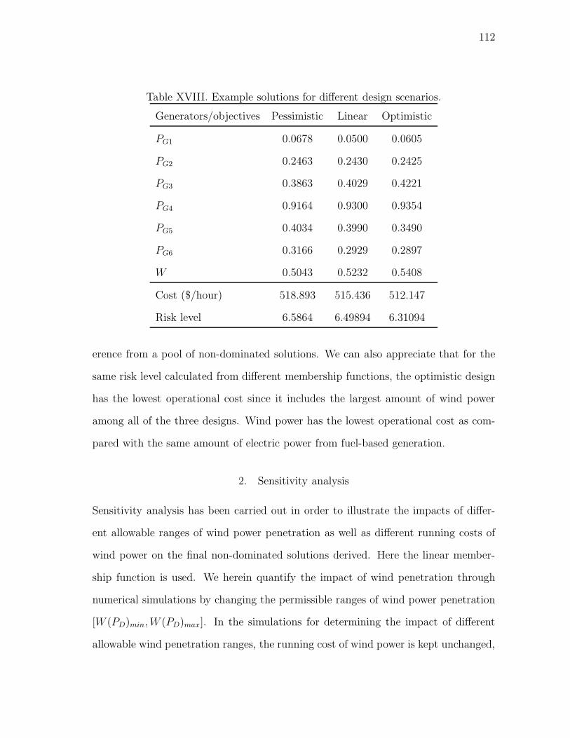
112
Table XVIII. Example solutions for different design scenarios.
Generators/objectives Pessimistic Linear Optimistic
PG1 0.0678 0.0500 0.0605
PG2 0.2463 0.2430 0.2425
PG3 0.3863 0.4029 0.4221
PG4 0.9164 0.9300 0.9354
PG5 0.4034 0.3990 0.3490
PG6 0.3166 0.2929 0.2897
W 0.5043 0.5232 0.5408
Cost ($/hour) 518.893 515.436 512.147
Risk level 6.5864 6.49894 6.31094
erence from a pool of non-dominated solutions. We can also appreciate that for the
same risk level calculated from different membership functions, the optimistic design
has the lowest operational cost since it includes the largest amount of wind power
among all of the three designs. Wind power has the lowest operational cost as com-
pared with the same amount of electric power from fuel-based generation.
2. Sensitivity analysis
Sensitivity analysis has been carried out in order to illustrate the impacts of differ-
ent allowable ranges of wind power penetration as well as different running costs of
wind power on the final non-dominated solutions derived. Here the linear member-
ship function is used. We herein quantify the impact of wind penetration through
numerical simulations by changing the permissible ranges of wind power penetration
[W (PD)min, W (PD)max]. In the simulations for determining the impact of different
allowable wind penetration ranges, the running cost of wind power is kept unchanged,

113
500 510 520 530 540 550 5600
2
4
6
8
10
12
14
16
18
20
Operational cost ($/hour)
Ris
k le
vel
Quadratic function (Pessimistic)Linear function (Neutral)Quadratic function (Optimistic)
Fig. 16. Pareto fronts obtained based on different membership functions
i.e., σ = 50$/p.u. In a similar fashion, in the simulations for examining the impact
of running costs of wind power, the penetration range of wind power is fixed, i.e.,
[W (PD)min, W (PD)max] = [10%∗PD, 20%∗PD]. The derived Pareto fronts are shown
in Figure 17 and Figure 18, respectively. From the figures, we can appreciate that the
non-dominated solutions vary with the different ranges of allowable wind penetration
as well as the running costs of wind power. In Figure 17, at the same risk level, the
design scenario with the largest value of maximum allowable wind penetration Wmax
has the lowest cost since the most portion of wind power is integrated. In Figure 18,
at the identical risk level, the scenario with the lowest running cost of wind power
results in the lowest overall cost since the same amount of wind power is integrated
with the lowest cost.

114
500 510 520 530 540 550 560 570 580 5900
2
4
6
8
10
12
14
16
18
20
Operational cost ($/hour)
Ris
k le
vel
[6%,16%][8%,18%][10%,20%]
Fig. 17. Pareto fronts obtained for different wind penetration ranges
3. Comparative studies
In order to conduct a quantitative assessment of the performance of a multi-objective
optimization algorithm, normally four major issues should be considered:
• Minimize the distance of the approximated Pareto front obtained from the tar-
get algorithm with respect to the true Pareto front. Since the true Pareto front
is unknown in most practical problems, this requirement can be interpreted
as increasing the accuracy of the obtained final solutions (i.e., to render the
obtained Pareto front as close to the true one as possible).
• Maximize the spread of the obtained solutions. It means that the diversity
of the solutions should be maximized in the optimization run by rendering the
distribution of the solutions as smooth and even as possible. Thus, the decision-

115
500 510 520 530 540 550 560 5700
2
4
6
8
10
12
14
16
18
20
Operational cost ($/hour)
Ris
k le
vel
Running cost = 40 $/p.u.Running cost = 50 $/p.u.Running cost = 60 $/p.u.
Fig. 18. Pareto fronts obtained for different running costs of wind power
maker will have more choices for different demands on decision.
• Maximize the number of elements of the Pareto-optimal set. The extent of the
estimated Pareto front should be increased, i.e., a wide range of non-dominated
solutions in objective space should be derived by the optimizer. For each objec-
tive, a sufficiently wide range of values should be covered by the non-dominated
solutions.
• Minimize the computational cost. Most of the MO optimization algorithms are
computationally expensive, thus the computational time is an important crite-
rion for measuring the efficacy of an algorithm in dealing with such problems.
Thus, certain quantitative metrics need to be defined in order to compare the
performance of different MO algorithms in a more objective fashion. A comparative

116
study is conducted to examine how competitive the proposed approach is in dealing
with the target problem. Comparison of Pareto front estimates is not a easy task
since it is unlikely to evaluate the quality of a Pareto front using any single measure.
Here, we use four measures to comprehensively assess the performance of different
optimizers in terms of accuracy, diversity, extent, and computational economy. Note
that all the following comparisons are conducted based on the neutral design scenario
with the original design parameters.
• C-metric: C-metric is quite often used to examine the quality of the Pareto
fronts obtained [66]. Let S1, S2 ⊆ S be two sets of decision solutions. The
C-metric is defined as the mapping between the ordered pair (S1, S2) and the
interval [0, 1]:
C(S1, S2) =|a2 ∈ S2; ∃a1 ∈ S1 : a1 a2|
|S2|(7.31)
Provided that C(S1, S2) = 1, all solutions in S2 are dominated by or equal to
solutions in S1. If C(S1, S2) = 0, then none of the solutions in S2 are covered
by S1. Both C(S1, S2) and C(S2, S1) should be checked in the comparison since
C-metric is not symmetrical in its arguments, i.e., the equation C(S1, S2) = 1−
C(S2, S1) does not necessarily always hold. Table XIX illustrates the comparison
of C-metric for different algorithms, where “O”, “F”, “S”, and “M” indicate the
original MOPSO, MOPSO only with f-gbest selection, MOPSO only with SPLS,
and MOMPSO, respectively.
• Spacing: The spacing metric is defined to measure the spread of the non-
dominated solutions. For instance, one of such metrics is to measure the range
variance of neighboring individuals in the set of non-dominated solutions [67].

117
Table XIX. Comparison of C-metric for different algorithms
C(M, O) C(O, M) C(M, F) C(F, M) C(M, S) C(S, M)
Best 1.0 0.1001 1.0 0.1427 1.0 0.1503
Worst 0.9899 0.0 0.9890 0.0 0.9811 0.0
Average 0.9993 0.0001 0.9905 0.0002 0.9880 0.0005
Median 0.9995 0.0001 0.9928 0.0002 0.9882 0.0005
Std. Dev. 0.0001 0.0001 0.0009 0.0001 0.0010 0.0002
It is defined as
SP =
√
√
√
√
1
n− 1
n∑
i=1
(d− di)2 (7.32)
where di = minj(|fi1(−→x )− f j
1 (−→x )| + |f i2(−→x ) − f j
2 (−→x )|), i, j = 1, . . . , n, d is the
mean of all di, and n is the number of non-dominated solutions found so far.
The larger the value is, the more unevenly the solution members are spaced.
If the value of SP is zero, all members in the Pareto front are equidistantly
distributed. Table XX illustrates the comparison of the spacing metric for
different algorithms. For simplicity of notation, here f-gbest is used to denote
the MOPSO only with f-gbest and SPLS represents the MOPSO only with
SPLS.
Table XX. Comparison of the spacing metric for different algorithms
Spacing MOPSO f-gbest SPLS MOMPSO
Best 0.0489 0.0403 0.0397 0.0389
Worst 0.1077 0.0996 0.0988 0.0767
Average 0.0526 0.0422 0.0418 0.0402
Median 0.0521 0.0412 0.0410 0.0375
Std. Dev. 0.2562 0.1131 0.0988 0.0612
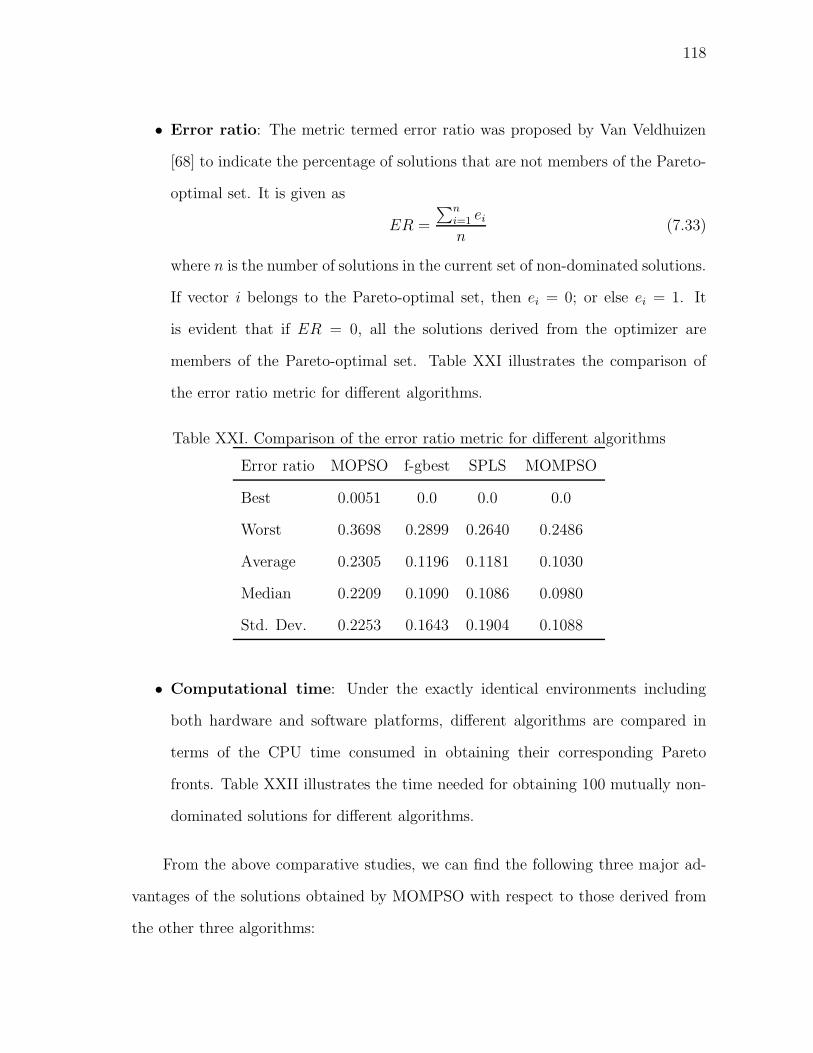
118
• Error ratio: The metric termed error ratio was proposed by Van Veldhuizen
[68] to indicate the percentage of solutions that are not members of the Pareto-
optimal set. It is given as
ER =
∑n
i=1 ei
n(7.33)
where n is the number of solutions in the current set of non-dominated solutions.
If vector i belongs to the Pareto-optimal set, then ei = 0; or else ei = 1. It
is evident that if ER = 0, all the solutions derived from the optimizer are
members of the Pareto-optimal set. Table XXI illustrates the comparison of
the error ratio metric for different algorithms.
Table XXI. Comparison of the error ratio metric for different algorithms
Error ratio MOPSO f-gbest SPLS MOMPSO
Best 0.0051 0.0 0.0 0.0
Worst 0.3698 0.2899 0.2640 0.2486
Average 0.2305 0.1196 0.1181 0.1030
Median 0.2209 0.1090 0.1086 0.0980
Std. Dev. 0.2253 0.1643 0.1904 0.1088
• Computational time: Under the exactly identical environments including
both hardware and software platforms, different algorithms are compared in
terms of the CPU time consumed in obtaining their corresponding Pareto
fronts. Table XXII illustrates the time needed for obtaining 100 mutually non-
dominated solutions for different algorithms.
From the above comparative studies, we can find the following three major ad-
vantages of the solutions obtained by MOMPSO with respect to those derived from
the other three algorithms:

119
Table XXII. Comparison of computational time for different algorithms (in seconds)
CPU time MOPSO f-gbest SPLS MOMPSO
Best 15.2 14.9 12.8 11.2
Worst 19.9 17.9 16.4 12.5
Average 17.5 16.0 13.1 11.7
Median 17.9 16.4 13.4 11.6
Std. Dev. 0.1024 0.0549 0.0602 0.0121
• Higher quality solutions are obtained using the MOMPSO. In the set of solutions
obtained using MOMPSO, most of them have better objective function values
than those derived from other approaches.
• The solutions of MOMPSO have better diversity characteristics. This is pri-
marily due to the several diversity retention mechanisms used:
– A useful distribution preservation measure adopted in this study is the
fuzzification mechanism used during the selection of global guide for each
particle in every generation;
– A local search scheme termed Synchronous Particle Local Search (SPLS)
is integrated into the original MOPSO in order to enhance the population
diversity and expedite the convergence speed;
– Niching and fitness sharing is used to preserve the population diversity by
preventing the population from falling into the detrimental genetic drift;
– In the archiving process, the individuals lying in less populated regions
of the objective have higher chance to be chosen than those in the highly
populated areas;

120
– A turbulence factor is added to the PSO operations, which may increase the
solution diversity by enhancing the randomness in a particle’s movements.
The diversity is preserved by MOMPSO while there is no guarantee that the
solutions obtained by objective aggregation approach will span over the entire
tradeoff surface.
• The computational time of MOMPSO is less than the other methods. The
SPLS mechanism incorporated reduces the computational expense due to its
capability of facilitating convergence speedup.
F. Summary
This chapter investigates the integration of wind power into conventional power net-
works and its impact on generation resource management. Wind power is environmen-
tally friendly since it is able to reduce the fossil fuel and natural gas consumption.
Also, wind power needs less operational cost since it does not consume fossil fuels
and natural gases. However, due to the intermittent and variable nature of the wind
power, it is usually quite difficult to determine how much wind power should be inte-
grated to ensure both power system security and operational cost reduction. In this
chapter, fuzzy representations of system security in terms of wind power penetration
level and operational costs are adopted in constructing economic dispatch models. A
multi-objective memetic particle swarm optimization (MOMPSO) algorithm is devel-
oped to derive the non-dominated Pareto-optimal solutions in terms of the specified
multiple design objectives. Different design scenarios can be formulated according to
dispatcher’s attitudes toward wind power integration with respect to risk and cost.
A numerical application example is used to illustrate the validity and applicability
of the developed optimization procedure. In the further investigations, probabilis-

121
tic methods may also be adopted to handle various uncertainties in power systems
including wind power penetration.

122
CHAPTER VIII
MULTI-CRITERIA DESIGN OF HYBRID POWER GENERATION SYSTEMS
BASED ON A MODIFIED PARTICLE SWARM OPTIMIZATION ALGORITHM
Multi-source hybrid power generation systems are a type of representative applica-
tions of the renewables’ technology. In this investigation, wind turbine generators,
photovoltaic panels, and storage batteries are used to build hybrid generation sys-
tems which are optimal in terms of multiple criteria including cost, reliability, and
emissions. Multi-criteria design facilitates the decision-maker to make more rational
evaluations. In this study, an improved particle swarm optimization algorithm is de-
veloped to derive these non-dominated solutions. Hybrid generation systems under
different design scenarios are designed based on the proposed approach. First, a grid-
linked hybrid system is designed without incorporating system uncertainties. Then,
adequacy evaluation is conducted based on probabilistic methods by accounting for
equipment failures, time-dependent sources of energy, and stochastic generation/load
variations. In particular, due to the unpredictability of wind speed and solar insola-
tion as well as the random load variation, time-series models are adopted to reflect
their stochastic characteristics. An adequacy evaluation procedure including time-
dependent sources is adopted. Sensitivity studies are also carried out to examine the
impacts of different system parameters on the overall design performance.
A. Introduction
With the increasing concerns on air pollution and global warming, the clean green
renewable sources of energy are expected to play more significant role in the global
energy future [5], [36], [77]. Most of them are environmentally benign and do not
contribute to the atmospheric pollution, acid rain, and global climate warming. Fur-

123
thermore, due to public support and government incentives over recent decades, they
are growing rapidly, not only in technical performance, but also in the breadth of
applications. The public attention has remained focused on these renewable tech-
nologies as environmentally sustainable and convenient alternatives. Among them,
wind power and solar power are the two most widely used renewable sources of energy
since they feature certain merits as compared with the conventional fossil-fuel-fired
generation. For instance, wind turbine generators (WTGs) generate no pollution and
they do not consume depleting fossil-fuels. Photovoltaic (PV) systems produce no
emissions, are durable, and demand minimal maintenance to operate. Unfortunately,
these renewable sources of energy are essentially intermittent and quite variable in
their output. Also, they require high capital costs. Thus, it is possible that power
fluctuations will be incurred since both power sources are highly dependent on the
weather conditions [76]. To mitigate or even cancel out the fluctuations, energy stor-
age technologies such as storage batteries (SBs) can be employed. SBs may absorb the
surplus power and provide the deficit power in different operating situations [71], [72].
As a result, hybrid generation systems have attracted much attention [74], [75], [78]–
[81]. However, besides the fluctuations of time-dependent sources, there are various
uncertainties existing in operations of such hybrid systems, e.g., possible equipment
failures and stochastic generation/load variations. Therefore, reliability evaluation for
the intended system using probabilistic methods is highly desired. In this investiga-
tion, adequacy evaluation theory is used in the design to ensure the system reliability
in the presence of generating-unit malfunctions. To reflect the stochastic charac-
teristics of wind and solar power, an autoregressive moving average (ARMA) time
series is used to model the wind speed and solar insolation in different time instants.
Furthermore, autoregressive integrated moving average (ARIMA) time series is used
to model the random variation of load demand. In this way, various uncertainties

124
including equipment failures and random generation/load variations are taken into
account in the system design, which is expected to enhance system reliability in the
face of different uncertainties.
In this chapter, we employ a multi-criteria approach to handle hybrid system de-
sign problems by taking into account multiple design objectives including economics,
reliability, and pollutant emissions. Multi-criteria design helps the decision-maker
reflect upon, articulate, and apply value judgments to determine reasonable trade-
offs and thus lead to recommendations of corresponding alternatives [70], [82]. Thus,
multi-criteria design provides a viable way to reach tradeoffs among these design
objectives with different preferences. Also, due to the high complexity and high non-
linearity of the design problem, a metaheuristics called particle swarm optimization
(PSO) is adopted and improved accordingly in order to derive a set of non-dominated
solutions with sufficient diversity for decision-making support. PSO has turned out
to be an outstanding optimizer due to its ability to elegantly handle difficult opti-
mization problems as well as its exceptional convergence performance.
The remainder of the chapter is organized as follows. Section B formulates
the hybrid system design problem including its multiple objectives coupled with a
set of design constraints. The proposed multiobjective particle swarm optimization
(MOPSO) algorithm is detailed in Section C. Simulation results and sensitivity stud-
ies for designing grid-linked hybrid systems without and with system uncertainties
consideration are presented in Section D and Section E, respectively. Finally, conclu-
sions are drawn and future research direction is suggested.

125
B. Problem Formulation
As shown in Figure 19, a typical hybrid generation system comprises different power
sources including wind turbine generators (WTGs), PV panels (PVs), and storage
batteries (SBs). These power sources have different impacts on cost, environment,
and reliability. In a hybrid generation system, they are integrated together and com-
plement one another in order to serve the load while satisfying certain economic, envi-
ronmental, and reliability criteria. The hybrid system can be operated autonomously
or connected to the utility grid whose power is from the conventional fossil-fuel-fired
generators (FFGs). Due to space restrictions, here only grid-linked system designs
will be discussed. The multi-criteria design of a stand-alone hybrid generation system
can be referred to [83].
WTGs
PV Panels
OtherRenewable
Sources
AC/DC
DC/DC
AC(DC)/DC
DC/AC
Storage Batteries
Dump Load
UtilityGrid
DC Bus AC Load Bus
Fig. 19. Configuration of a typical hybrid generation system
The objective of this study is to achieve hybrid generation systems, which should
be appropriately designed in terms of economic, reliability, and environmental mea-
sures subject to physical and operational constraints/strategies. Two design scenarios
are investigated, i.e., grid-linked hybrid generation systems without and with uncer-
tainties consideration. Here we start with the discussion of a hybrid system design

126
without considering uncertainties. That is, neither generator failures nor stochas-
tic generation/load variations is considered in the design. Some of the calculations
formulated in this section are applicable to the hybrid system design incorporating
adequacy evaluation including uncertainties discussed in Section F.
1. Design objectives
• Objective 1: Costs
Proper cost estimation is crucial to the success of projects like hybrid generation
system design [74], [75]. In this study, the total cost COST ($/year) includes
initial cost, operational and maintenance (OM) cost for each type of power
source, and the salvage value of each equipment should be deducted:
COST =
∑
i=w,s,b(Ii − SPi+ OMPi
)
Np
+ Cg (8.1)
where w, s, b indicates the wind power, solar power, and battery storage, respec-
tively; Ii, SPi, OMPi
are the initial cost, present worth of salvage value, and
present worth of operation and maintenance cost for equipment i, respectively;
Np(year) is the life span of the project; and Cg is the annual cost for purchasing
power from the utility grid. Here we assume that the life time of the project
does not exceed those of both WTGs and PV arrays.
1) For the WTGs,
Iw = αwAw (8.2)
where αw($/m2) is the initial cost of WTGs; the present worth of the total
salvage value is
SPw= SwAw(
1 + β
1 + γ)Np (8.3)

127
where Sw($/m2) is the salvage value of WTGs per square meter, β and γ are
the inflation rate and interest rate, respectively; the present worth of the total
operation and maintenance cost (OM) in the project life time is
OMPw= αOMw
∗ Aw ∗
Np∑
i=1
(1 + ν
1 + γ)i (8.4)
where αOMw($/m2/year) is the yearly OM cost per unit area and ν is the esca-
lation rate.
2) For the PV panels, the initial cost is
Is = αsAs (8.5)
where αs($/m2) is the initial cost; the present worth of the total salvage value
is
SPs= SsAs(
1 + β
1 + γ)Np (8.6)
where Ss($/m2) is the salvage value of PVs per square meters of PV panels; the
present worth of the total operation and maintenance cost (OM) in the project
life time is
OMPs= αOMs
∗ As ∗
Np∑
i=1
(1 + ν
1 + γ)i (8.7)
where αOMs($/m2/year) is the yearly OM cost per unit area and ν is the esca-
lation rate.
3) For the storage batteries, since their life span is usually shorter than that of
the project, the total present worth of capital investments can be calculated as

128
follows:
Ib = αb ∗ Pbcap∗
Xb∑
i=1
(1 + ν
1 + β)(i−1)Nb (8.8)
where Nb is the life span of SBs; Xb is the number of times to purchase the
batteries during the project life span Np; the salvage value of SBs is ignored in
this study; and the present worth of the total OM cost in the project life time
is calculated as follows:
OMpb= αOMb
∗ Pbcap∗
Np∑
i=1
(1 + ν
1 + γ)i (8.9)
where αOMb($/kWh/year) is the yearly OM cost per kilowatthour.
4) For the grid-linked system design, the annual cost for purchasing power from
the utility grid can be calculated as follows:
Cg =
T∑
t=1
Pg,t ∗ ϕ (8.10)
where Pg,t($/year) is the power purchased from the utility at hour t; ϕ($/kWh)
is the grid power price; and T (8760 hours) is the operational duration under
consideration.
• Objective 2: Reliability
Reliability is used to assess the quality of load supply. Here Energy Index of
Reliability (EIR) is used to measure the reliability of each candidate hybrid sys-
tem design. EIR can be calculated from Expected Energy Not Served (EENS)
as follows:
EIR = 1−EENS
E(8.11)
The EENS(kWh/year) for the duration under consideration T (8760 hours)

129
can be calculated as follows:
EENS =
T∑
t=1
(Pbmin− Pbsoc
(t)− Psup(t)) ∗ U(t) (8.12)
where U(t) is a step function, which is zero when the supply exceeds or equals
to the demand, and equals to one if there is insufficient power in period t; Pd(t)
is the load demand during hour t, Psup(t) = Ptotal(t)−Pd(t) is the surplus power
in hour t, Ptotal(t) is the total power from WTGs, PVs, and FFGs during hour
t:
Ptotal(t) = Pw(t) + Ps(t) + Pg(t) (8.13)
Pbsoc(t) is the battery charge level during hour t, and Pbmin
is the minimum
permitted storage level, the term Pbsoc(t)− Pbmin
indicates the available power
supply from batteries during hour t; and provided that there is insufficient power
in hour t,
Pg(t) = κ ∗ (Pd(t)− Pw(t)− Ps(t)− Pb(t)) (8.14)
where κ ∈ [0, 1] indicates the portion of purchased power with respect to the
hourly insufficient power; or else, Pg(t) = 0. Note that no equipment failures and
unexpected load deviations are considered in calculating the EENS, which in
this design is all contributed by the fluctuations of renewable power generation.
• Objective 3: Pollutant emissions
With the increasing concerns on environment protection, there are stricter regu-
lations on pollutant emissions. The most important emissions considered in the
power generation industry due to their highly damaging effects on the ecological
environment are sulfur dioxide (SO2) and nitrogen oxides (NOx). These emis-
sions can be modeled through functions that associate emissions with power
production for generating units. They are dependent on fuel consumption and

130
take the quadratic form:
PE = α + β ∗T
∑
t=1
Pg,t + γ ∗ (T
∑
t=1
Pg,t)2 (8.15)
where α, β, and γ are the coefficients approximating the generator emission
characteristics.
2. Design constraints
Due to the physical or operational limits of the target system, there is a set of con-
straints that should be satisfied throughout system operations for any feasible solu-
tion.
• Constraint 1: Power balance constraint
For any period t, the total power supply from the hybrid generation system must
supply the total demand Pd with a certain reliability criterion. This relation
can be represented by
Pw(t) + Ps(t) + Pb(t) + Pg(t) ≥ (1− R)Pd(t) (8.16)
Pw(t) + Ps(t) + Pb(t) + Pg(t)− Pdump(t) ≤ Pd(t) (8.17)
where Pw, Ps, Pb, Pg, Pdump(t), and Pd are the wind power, solar power,
charged/discharged battery power, power bought from grid, dumped power,
and total load demand, respectively; R is the ratio of the maximum permissible
unmet power with respect to the total load demand in each time instant. The
transmission loss is not considered in this investigation.
The output PWTG (kW/m2) from WTGs for wind speed Vt can be calculated

131
as
PWTG =
0, Vt < Vci
a ∗ V 3t − b ∗ Pr, Vci ≤ Vt < Vr
Pr, Vr ≤ Vt ≤ Vco
0 Vt > Vco
(8.18)
where a = Pr
V 3r −V 3
ci
, b =V 3
ci
V 3r −V 3
ci
, Pr is the rated power, Vci, Vr, and Vco are the
cut-in, rated, and cut-out wind speed, respectively. The real electric power from
WTGs can be calculated as follows:
Pw = PWTG ∗ Aw ∗ ηw (8.19)
where Aw is the total swept area of WTGs and ηw is the efficiency of WTGs.
The output power Ps(kW ) from PV panels can be calculated as follows:
Ps = H ∗ As ∗ ηs (8.20)
where H(kW/m2) is the horizontal irradiance, As is the PV area, and ηs is the
efficiency of PV panels.
• Constraint 2: Bounds of design variables
The swept area of WGTs should be within a certain range:
Awmin≤ Aw ≤ Awmax
(8.21)
Similarly, the area of PV arrays should also be within a certain range:
Asmin≤ As ≤ Asmax
(8.22)
The state of charge (SOC) of storage batteries Pbsocshould not exceed the capac-
ity of storage batteries Pbcapand should be larger than the minimum permissible

132
storage level Pbmin; the total SB capacity should not exceed the allowed stor-
age capacity Pbcapmax; and the hourly charge or discharge power Pb should not
exceed the hourly inverter capacity Pbmax. As a result,
Pbmin≤ Pbsoc
≤ Pbcap(8.23)
0 ≤ Pbcap≤ Pbcapmax (8.24)
Pb ≤ Pbmax(8.25)
The amount of power bought from utility grid should be within a certain range:
Pgmin≤
T∑
t=1
Pg,t ≤ Pgmax, (8.26)
where Pgminand Pgmax
are the minimum and maximum power allowed to be
bought from the utility grid, respectively.
The coefficient κ indicates the portion of purchased power from utility grid with
respect to the insufficient power:
0 ≤ κ ≤ 1 (8.27)
3. Problem statement
In summary, for this grid-linked system design, the objective of optimum design for re-
newable hybrid generation system is to simultaneously minimize COST (Aw, Sw, Pbcap, κ)
and E(Aw, Sw, Pbcap, κ), as well as maximize EIR(Aw, Sw, Pbcap
, κ), subject to the con-
straints (8.16)–(8.27). The design parameters that should be derived include WTG
swept area Aw(m2), PV area As(m2), total battery capacity Pbcap
(kWh), and the
ratio of power purchased from grid κ.

133
4. Operation strategies
The power outputs from WTGs and PVs have the highest priorities to feed the load.
Only if the total power from wind and solar systems is insufficient to satisfy the load
demand, the storage batteries can be discharged a certain amount of energy to supply
the load. If there is still not enough power to supply the load, a certain amount of
power will be purchased from the utility grid. That is, the grid power has the lowest
priority to feed the load. Furthermore, if there is any excess power from WTGs and
PVs, the batteries will be charged to store a certain permissible amount of energy for
future use. If there is surplus power from WTGs and PVs even after feeding the load
and charging the SBs, the dump load will consume the spilled power.
C. The Proposed Approach
In this study, a Constrained Mixed-Integer Multi-Objective PSO (CMIMOPSO) is
developed to derive a set of non-dominated solutions by appropriately combining
different sources of energy subject to certain constraints.
1. CMIMOPSO
• Mixed-integer PSO: Since the target problem involves optimization of system
configuration, integer numbers are used to indicate the unit sizing. The standard
PSO is in fact a real-coded algorithm, thus some revisions are needed to enable it
to deal with the binary-coded optimization problem. In the discrete binary PSO
[32], the relevant variables are interpreted in terms of changes of probabilities.
A particle flies in a search space restricted to zero and one in each direction
and each vid represents the probability of member xid taking value 1. The
update rule governing the particle flight speed can be modified accordingly by

134
introducing a logistic sigmoid transformation function:
S(vid) =1
1 + e−vid
(8.28)
The velocity can be updated according to this rule: If rand() < S(vid), then
xid = 1; or else xid = 0. The maximum allowable velocity Vmax is desired to
limit the probability that member xid will take a one or zero value. The smaller
the Vmax is, the higher the chance of mutation is for the new individual.
• Multi-objective PSO: In this study, since a multi-objective optimization prob-
lem is concerned, the standard PSO algorithm is also modified accordingly to
facilitate a multi-objective optimization approach, i.e., multi-objective particle
swarm optimization (MOPSO). The Pareto-dominance concept is used to ap-
praise the fitness of each particle and thus determine which particles should be
chosen as the non-dominated solutions. For this purpose, the archiving mecha-
nism is used to store the non-dominated solutions throughout the optimization
process. The best historical solutions found by the optimizer are absorbed con-
tinuously into the archive as the non-dominated solutions generated in the past.
Furthermore, to enhance the solution diversity, some diversity preserving mea-
sures such as fuzzified global best selection, and niching and fitness sharing are
taken [84].
• Constrained PSO: In the proposed method, a natural constraint checking pro-
cedure called rejecting strategy is adopted to deal with the imposed constraints.
When an individual is evaluated, the constraints are first checked to determine
if it is a feasible candidate solution. If it satisfies all of the constraints, it is
then compared with the non-dominated solutions in the archive. The concept
of Pareto dominance is applied to determine if it is eligible to be chosen to

135
store in the archive of non-dominated solutions. As long as any constraint is
violated, the candidate solution is deemed infeasible. This procedure is simple
to implement, but it turned out to be quite effective in ensuring the solution
feasibility while not significantly decreasing the search efficiency.
2. Representation of candidate solutions
The design variables including WTG swept area, PV area, amount of power purchased
from the grid, and total SB capacity are encoded as the position value in each dimen-
sion of a particle. Several member positions indicate the coordinate of the particle in
a multi-dimensional search space. Each particle is considered as a potential solution
to the optimal design problem, since each of them represents a specific configuration
of the hybrid generation system. Excluding Pbcap, all the remaining positions are
real-coded. The i-th particle (i.e., candidate design) Di can be represented as follows:
Di = [Pw,i, Ps,i, Pbcap,i, κi], i = 1, 2, . . . , N (8.29)
where κ is ratio of power bought from the grid with respect to the deficit power, and
the total SB capacity Pbcapis encoded using three binary bits.
3. Data flow of the optimization procedure
The computational procedure of the propose method is as follows:
• Step 1: Specify the lower and upper bounds of WTG swept area, area of PV
panels, number of batteries, and other pre-determined parameters.
• Step 2: Randomly generate a population of particles. The speed and position
of each particle should be initialized such that all the particles locate within the
feasible search space.

136
• Step 3: Evaluate each particle Di in the population based on the concept of
Pareto-dominance.
• Step 4: Store the non-dominated solutions found so far in the archive.
• Step 5: Initialize the memory of each particle where a single personal best pbest
is stored. The memory is contained in another archive.
• Step 6: Increase the iteration number by one.
• Step 7: Choose the personal best position pbest for each particle based on the
memory record; Choose the global best gbest from the fuzzified region using
binary tournament selection [84]. The niching and fitness sharing mechanism is
also applied in order to enhance solution diversity.
• Step 8: Update the member velocity v of each individual Di. For the real-
encoded design variables,
v(t+1)id
= χ ∗ (w ∗ v(t)i + c1 ∗ rand() ∗ (pbestid − P
(t)Gid
)
+ c2 ∗ Rand() ∗ (gbestd − P(t)Gid
)),
i = 1, . . . , N ; d = 1, 2. (8.30)
• Step 9: Update the member position of each particle Di based on (8.29). For
real-coded variables,
D(t+1)id
= D(t)id
+ v(t+1)id
(8.31)
For the binary-encoded design variable, update the member position based on
the updating rule for discrete variables discussed in Subsection D.1.
Following this, add the turbulence factor into the current position. For all the

137
positions,
D(t+1)id
= D(t+1)id
+ RT D(t+1)id
(8.32)
where RT is the turbulence factor, which is used to enhance the solution diversity
by refraining the search from undesired premature convergence.
• Step 10: Update the archive which stores non-dominated solutions according to
Pareto-optimality based selection criteria [84].
• Step 11: If the current individual is dominated by the pbest in the memory,
then keep the pbest in the memory; Otherwise, replace the pbest in the memory
with the current individual.
• Step 12: If the maximum number of iterations is reached, then go to Step 13;
Otherwise, go to Step 6.
• Step 13: Print out a set of Pareto-optimal solutions from the archive as the
final possible system configurations.
D. A Case Study: System Design Without Incorporating Uncertainties
In this section, the tradeoff solutions are derived for a grid-linked hybrid system
without incorporating system uncertainties, and some sensitivity studies are carried
out.
1. System parameters
The data used in the simulation program are listed in Table XXIII [75]. The hourly
wind speed patterns, the hourly insolation conditions, and the hourly load profile are
shown in Figure 20. These time-series data will be used by the ARMA model [73] to
derive forecasted wind speed and solar insolation, which are then used to calculate

138
the available wind power, solar power, and the insufficient or surplus power at each
time instant.
1 2 3 4 5 6 7 8 9 10 11 12 13 14 15 16 17 18 19 20 21 22 23 244
5
6
7
Win
d sp
eed
(m/s
ec)
1 2 3 4 5 6 7 8 9 10 11 12 13 14 15 16 17 18 19 20 21 22 23 240
0.25
0.5
0.75
1
Inso
latio
n (k
W/m
2 )
1 2 3 4 5 6 7 8 9 10 11 12 13 14 15 16 17 18 19 20 21 22 23 240
1020304050
Hours of a day (hour)
Load
dem
and
(kW
)
Fig. 20. Hourly mean wind speed, insolation, and load profiles
2. PSO parameters
In the simulations, both the population size and archive size are set to 100, and the
maximum number of iterations is set to 500. The acceleration constants c1 and c2
are chosen as 1. Both turbulence factor and niche radius are set to 0.02. The inertia
weight factor w decreases when the number of generations increases:
w = wmax −wmax − wmin
itermax
× iter (8.33)
where itermax is the maximum number of iterations and iter is the current number
of iterations. This mechanism helps achieve the balance between exploration and
exploitation in the search process. The simulation program is coded using C++ and
executed in a 2.20 GHz Pentium-4 processor.

139
3. Simulation results
The Pareto-optimal fronts evolved using the proposed approach for bi- and tri-objective
optimization problems are shown in Figure 21, and two illustrative non-dominated
solutions are listed in Table XXIV.
Fig. 21. Pareto fronts for bi- and tri-objective optimization scenarios
4. Sensitivity to system parameters
Here the sensitivity analysis is carried out to examine the effects of changing the
values of certain system parameters on the final non-dominated solutions derived.
For instance, the mean wind speeds are changed by different multiplication factors
(MFs), and different economic rates are also examined. The results are illustrated
in Figure 22 and Figure 23, respectively. From Figure 22, we can appreciate the
importance of site locations for a wind power plant. The simulation results shown in
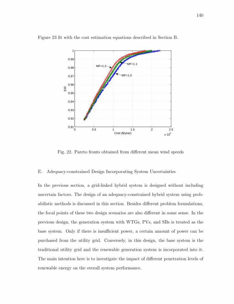
140
Figure 23 fit with the cost estimation equations described in Section B.
0 0.5 1 1.5 2 2.5
x 104
0.91
0.92
0.93
0.94
0.95
0.96
0.97
0.98
0.99
1
Cost ($/year)
EIR
MF=1.1
MF=1.0
MF=1.2
Fig. 22. Pareto fronts obtained from different mean wind speeds
E. Adequacy-constrained Design Incorporating System Uncertainties
In the previous section, a grid-linked hybrid system is designed without including
uncertain factors. The design of an adequacy-constrained hybrid system using prob-
abilistic methods is discussed in this section. Besides different problem formulations,
the focal points of these two design scenarios are also different in some sense. In the
previous design, the generation system with WTGs, PVs, and SBs is treated as the
base system. Only if there is insufficient power, a certain amount of power can be
purchased from the utility grid. Conversely, in this design, the base system is the
traditional utility grid and the renewable generation system is incorporated into it.
The main intention here is to investigate the impact of different penetration levels of
renewable energy on the overall system performance.

141
0 0.5 1 1.5 2 2.5 3
x 104
0.9
0.95
1
Cost ($/year)
EIR
Different Interest Rates
0 0.5 1 1.5 2 2.5 3
x 104
0.9
0.95
1
Cost ($/year)
EIR
Different Escalation Rates
γ=0.05
γ=0.12
γ=0.19
ν=0.19
ν=0.12
ν=0.05
Fig. 23. Pareto fronts obtained from different economic rates
Probabilistic methods are now being used more widely in power system planning
and operations due to a variety of uncertainties involved. For instance, adequacy
evaluation is an important component to ensure proper operations of power systems
in the presence of various uncertainties. Adequacy analysis of hybrid generating sys-
tems including time-dependent sources has been investigated in [15], [17], [18]. Here
an efficient reliability evaluation technique proposed in [15] is used to calculate the
reliability indices including Expected Unserved Energy (EUE), Loss of Load Expec-
tation (LOLE), and Loss of Load Frequency (LOLF), which are three fundamental
indices for adequacy assessment of generating systems. The main idea of this method
is to divide the generating system into a subsystem including all the conventional
units and a set of subsystems each of which contains a possibly fluctuating uncon-
ventional source. Here all the adequacy indices are calculated based on the analytical
method proposed in [15], which is also introduced in Chapter V.

142
1. Problem formulation
In this design scenario, only WTGs and PVs are used. Thus, the total cost COST ($/year)
can be changed as follows:
COST =
∑
i=w,s(Ii − SPi+ OMPi
)
Np
(8.34)
Here the cost for generating FFG power is excluded from the total cost calculation in
order to examine the impact of wind and solar power penetration level on the overall
system design in a more explicit fashion.
The real power balance constraint in this design scenario can be represented by
Pwt+ Pst
+ Pgt≥ (1− R)Pdt
(8.35)
Pwt+ Pst
+ Pgt− Pdumpt
≤ Pdt(8.36)
Furthermore, due to the fluctuations of available wind and solar power coupled
with possible generator failures, the loss of load may be caused. To ensure a certain
degree of system reliability, the indices of LOLE and LOLF should also be fulfilled
besides the maximization of EIR.
LOLE ≤ LOLEmax (8.37)
where LOLEmax is the maximum LOLE allowed. In a similar manner, LOLF should
also be less than or equal to the maximum value LOLFmax:
LOLF ≤ LOLFmax (8.38)
As we can see, in this study one reliability index (EUE) is used as the design
objective and the other two (LOLE and LOLF) are used as design constraints to
ensure the generating system adequacy, which can be computed simultaneously.

143
In this scenario, the objective of optimum design for hybrid generating system
with time-dependent sources is to simultaneously minimize COST (Aw, As) as well as
maximize EIR(Aw, As), subject to the constraints (8.21)–(8.22) coupled with (8.35)–
(8.38). The design parameters that should be derived include total WTG swept area
Aw(m2) and total PV area As(m2).
2. Simulation results
Three identical two-state FFGs are used together with multiple wind/solar generating
units. Since solar power is much less prone to equipment failures, failures of PV
cells are not considered in this investigation. In simulations, four identical WTGs
are considered during the hybrid system design, and the capacity of each WTG is
determined by the candidate solution under consideration. The rated FFG power
(PFFG) is 20 kW , and the reliability characteristics of each type of generating units
are as follows: FFG failure rate (λFFG) is 0.1 day−1, FFG repair rate (µFFG) is 0.9
day−1, WTG failure rate (λWTG) is 0.1 day−1, and WTG repair rate (µWTG) is 0.4
day−1. Furthermore, LOLEmax and LOLFmax are set 1.5 h/week and 1 occ./week,
respectively.
The computational procedure used is basically same as in the previous design,
but some minor changes are needed to fit it into the current design scenario. For in-
stance, the particle representation and design constraints should be modified accord-
ingly. The Pareto-optimal front evolved in this design scenario using the proposed
approach is shown in Figure 24. The decision-maker can choose a design solution
from the derived set of non-inferior solutions based on the specific design requirement
or preference. Two illustrative non-dominated solutions are listed in Table XXV. We
can appreciate that the improvement of one objective is at the expense of deteriora-
tion of another objective. Thus, for any specific system design, a tradeoff between

144
these two objectives should be reasonably made.
0 0.5 1 1.5 2 2.5 3
x 104
0.91
0.92
0.93
0.94
0.95
0.96
0.97
0.98
0.99
1
Cost ($/year)
EIR
Fig. 24. Pareto front indicating a set of non-inferior design solutions
To examine the impacts of different wind speeds and insolations on the Pareto-
optimal solutions derived, sensitivity studies are carried out. Figure 25 and Figure 26
show the tradeoff surfaces obtained in different scenarios in terms of wind speeds and
solar insolations, respectively. Note that during the simulations, when different wind
speeds are examined, the original insolation value is used. Likewise, when different
insolations are examined, the original wind speed value is used. We can appreciate
that at the same reliability level, the generating systems with the highest speed and
insolation result in the lowest costs when compared with scenarios with lower wind
speed and insolation. Thus, this confirms the previous observation that it is crucial to
properly select power plant location when renewable sources of energy are involved.
Usually plant sites with richer renewable sources of energy can cause lower generation
costs.

145
0 0.5 1 1.5 2 2.5 3 3.5 4
x 104
0.91
0.92
0.93
0.94
0.95
0.96
0.97
0.98
0.99
1
Cost ($/year)
EIR
Halve the wind speed
The original wind speed
Double the wind speed
Fig. 25. Impacts of different wind speeds on Pareto fronts derived
Next, the stochastic nature of load is considered, which is modeled through a
time-series method called Autoregressive Integrated Moving Average (ARIMA) [69].
Two illustrative non-dominated solutions are listed in Table XXVI, and Figure 27
shows the tradeoff surface in this design scenario. We can appreciate that the stochas-
tic characteristic of load demand induces somewhat more costs for ensuring the same
reliability level. This is understandable since random variations of load may compro-
mise the system reliability. Also, Figure 28 shows the impacts of different wind speeds
on the Pareto-optimal solutions derived. It further verifies the previous observation
on the plant site selection.
F. Summary
Distributed generation using sustainable clean green power promises to considerably
restructure the energy industry, which is evolving from fossil fuels towards renew-

146
0 0.5 1 1.5 2 2.5 3
x 104
0.91
0.92
0.93
0.94
0.95
0.96
0.97
0.98
0.99
1
Cost ($/year)
EIR
Halve the insolation
The original insolation
Double the insolation
Fig. 26. Impacts of different insolations on Pareto fronts derived
ables [77]. Meanwhile, there are many open-ended problems in this field awaiting
to be resolved. In this chapter, a hybrid power generation system including wind
power and solar power is designed on the basis of cost, reliability, and emission cri-
teria. A set of tradeoff solutions is obtained using the multi-criteria metaheuristic
method which offers many design alternatives to the decision-maker. Moreover, in
one of the designs, system uncertainties such as equipment failures and stochastic
generation/load variations are considered by conducting adequacy evaluation based
on probabilistic methods. In particular, the stochastic generation/load variations are
modeled through time-series methods. Numerical simulations are used to illustrate
the applicability and validity of the proposed MOPSO-based optimization procedure,
and some sensitivity studies are also carried out. In the future studies, other more
complicated design scenarios may be incorporated into system designs.

147
0 0.5 1 1.5 2 2.5 3
x 104
0.91
0.92
0.93
0.94
0.95
0.96
0.97
0.98
0.99
1
Cost ($/year)
EIR
Fig. 27. Pareto front indicating a set of non-inferior design solutions considering
stochastic load variations
0 0.5 1 1.5 2 2.5 3 3.5 4
x 104
0.91
0.92
0.93
0.94
0.95
0.96
0.97
0.98
0.99
1
Cost ($/year)
EIR
Halve the wind speed
The original wind speed
Double the wind speed
Fig. 28. Impacts of different wind speeds on Pareto fronts derived considering stochas-
tic load variations

148
Table XXIII. The data used in the simulation programSystem parameters Values
Efficiency of WTG (ηw) 50%Efficiency of PV (ηs) 16%Efficiency of SB (ηb) 82%Inflation rate (β) 9%Interest rate (γ) 12%Escalation rate (ν) 12%Life span of project (Np) 20 yearsLife span of WTG (Nw) 20 yearsLife span of PV (Ns) 22 yearsLife span of SB (Nb) 10 yearsPV panel price (αs) 450$/m2
WTG price (αw) 100$/m2
SB price (αb) 100$/KWhPV panel salvage value (Ss) 45$/m2
WTG salvage value (Sw) 10$/m2
OM costs of WTG (αOMw) 2.5$/m2/yearOM costs of PV panel (αOMs) 4.3$/m2/yearOM costs of SB (αOMb
) 10$/KWhCut-in wind speed (Vci) 2.5 m/sRated wind speed (Vr) 12.5 m/sCut-out wind speed (Vco) 20.0 m/sRated WTG power (Pr) 4.0 kWPeriod under observation (T ) 8760 hoursMaximum swept area of WTGs (Awmax) 10, 000m2
Minimum swept area of WTGs (Awmin) 400m2
Maximum area of PV panels (Asmax) 200m2
Minimum area of PV panels (Asmin) 8, 000m2
Maximum conversion capacity (Pbmax) 3 kWh
Minimum storage level (Pbmin) 3 kWh
Rated battery capacity (Pbr) 8 kWh
Maximum total SB capacity (Pbmax) 40 kWh
Price of utility grid power (ϕ) 0.12$/kWh

149
Table XXIV. Two illustrative non-dominated solutions for tri-objective optimization
Variables/objectives Design 1 Design 2
Aw(m2) 810 680
As(m2) 40 40
Pbcap(kWh) 16 16
κ 0.34 0.58
Cost ($/year) 7,919.55 7,012.10
EIR 0.9579 0.9521
Emissions (ton/year) 17.0836 59.8295
Table XXV. Two illustrative system configurations for adequacy-constrained design
Variables Design 1 Design 2
Aw(m2) 880 1020
As(m2) 40 160
Cost ($/year) 7191.5 11233
EIR 0.9451 0.9653
Table XXVI. Two illustrative system configurations for adequacy-constrained design
with load forecasting
Variables Design 1 Design 2
Aw(m2) 880 1020
As(m2) 40 160
Cost ($/year) 7312 11418
EIR 0.9451 0.9653

150
CHAPTER IX
CAPACITY CREDIT ESTIMATION OF WIND POWER: FORMULATION AS
AN OPTIMIZATION PROBLEM
Significant amounts of wind power are being integrated into power grids in recent
years. However, due to intermittent characteristic of wind power, it is usually dif-
ficult to determine the appropriate penetration level to ensure a specified reliability
requirement. For this purpose, the proper calculation of wind power capacity credit
(WPCC) is of particular importance which is useful in both planning and operation
stages of hybrid power systems with multiple power sources. The capacity credit of
wind power is usually calculated based on a reliability index termed Loss of Load Ex-
pectation (LOLE). WPCC is the amount of wind power which is able to achieve the
LOLE identical to the dispatchable power sources. In this study, WPCC estimation
is formulated as an optimization problem, and an intelligent search method called
particle swarm optimization is used to automatically search out the WPCC. It has
turned out to be a viable scheme in estimating WPCC.
A. Introduction
In planning generation facilities, the planners are faced with the question of giving
appropriate credit for generating capacity from intermittent sources like wind. Es-
timation of wind power capacity credit (WPCC) due to the intermittency of wind
availability is not a sufficiently investigated area so far, and it is also a challenging
task. There are several definitions on the wind power capacity credit, one of which is
based on the system load carrying capability. Since the penetrated wind power can
be seen as “negative load”, an increase in load carrying capability can be achieved
while still ensuring the original level of system reliability. The amount of this extra

151
load is used as a measure for capacity credit of wind power in this study.
Probabilistic methods have been more widely used in power system planning,
since they are capable of incorporating various system uncertainties [1]. The estima-
tion of wind power capacity credit is based on the reliability indices such as loss of
load expectation (LOLE). Here an analytical procedure based on the mean capacity
outage table is used for LOLE calculation. A trial-and-error method has been used
to find out the WPCC in our previous work [85]. However, due to the complexity and
nonlinearity of this problem, this method is usually not time-efficient since it demands
tedious trial effort. In this work, for the first time WPCC estimation is formulated as
an optimization problem, and an automatic intelligent search method is used to search
for the WPCC value in a much more efficient fashion. Particle swarm optimization [8]
is used for this purpose due to its proven high search efficiency in dealing with highly
complex and nonlinear problems. Furthermore, a numerical study based on a practi-
cal power system is conducted to indicate the viability of the proposed method. The
method is also flexible and opens up other possibilities like incorporating constraints,
if needed, while computing WPCC.
The remainder of the chapter is organized as follows. Section B presents the
concept and calculation of wind power capacity credit based on reliability evaluation
for hybrid power-generating systems. In Section C, the proposed PSO-based WPCC
estimation method is discussed in detail. Simulation results and analysis are presented
and discussed in Section D. Finally, the chapter is wrapped up with the conclusion
and future research suggestion.

152
B. Wind Power Capacity Credit
Due to the wind speed variations, the output of wind turbine generator (WTG)
does not equal its rated capacity in most time periods. This creates difficulties for
system planners since the effective capacity of WTG needs to be determined based on
certain criteria. Quite often, reliability indices are used to measure the impact of the
wind power penetration. Thus, in calculating wind power capacity credit, reliability
indices such as loss of load expectation over the specified observation horizon are
used to ensure that power system meets the reliability level after the wind power is
integrated.
The reliability analysis of hybrid generating systems including time-dependent
sources has been investigated through different methods including analytical, simu-
lation, and artificial intelligence methods [14]–[18], [86]. These proposed reliability
evaluation techniques are usually intended to calculate the reliability indices includ-
ing Expected Energy Not Supplied (EENS), Loss of Load Expectation (LOLE), and
Loss of Load Frequency (LOLF), which are three fundamental indices for adequacy
assessment of power-generating systems. In the calculation of wind power capacity
credit, usually LOLE is used as the reliability index. Thus in this chapter only LOLE
will be discussed.
Assume the load is represented as a chronological sequence of NT discrete values
Lt for successive time steps t = 1, 2, . . . , NT . Each time step has equal duration
∆T = TNT
where T is the entire period of observation. The LOLE of the power
system without wind power integration can be calculated as follows:
LOLE = ∆T
NT∑
t=1
Pf(Cgt< Lt) (9.1)
where Pf is the loss of load probability, Cgtis the capacity of conventional power

153
sources, Lt is the load demand in period t. The LOLE with wind power penetration
can be calculated as follows:
LOLE = ∆T
NT∑
t=1
Pf [(Cgt+ Cwt
) < Lt] (9.2)
where Cwtis the effective wind power at time instant t. In the above definition, the
term Cgt+ Cwt
indicates the effective total system capacity (that is, the summation
of conventional sources of power and wind power at time instant t).
From the definition of reliability-based wind power capacity credit, we need to
ensure the identical power system reliability (i.e., LOLE in most cases) in both situ-
ations with and without wind power penetration:
NT∑
t=1
Pf(Cgt< Lt) =
NT∑
t=1
Pf [(Cgt+ Cwt
) < (Lt + E)] (9.3)
where E is the capacity credit of wind power we need to find out.
C. The Proposed Method
In the proposed method, WPCC estimation is formulated as an optimization problem,
which can be solved by intelligent search algorithms.
1. Problem formulation
The design objective is to find the WPCC variable E, which is able to minimize
the difference between LOLEs of the power system with and without wind power
generation. Thus, the objective function in PSO is defined as (9.4), which is to be
minimized:
F = (
NT∑
t=1
Pf(Cgt< Lt)−
NT∑
t=1
Pf [(Cgt+ Cwt
) < (Lt + E)])2 (9.4)

154
This is a highly nonlinear and complex function, since LOLE calculation is needed
for each potential solution.
A set of stochastic search algorithms is able to handle this optimization prob-
lem. Here particle swarm optimization (PSO) is used, which is a population-based
intelligent search procedure inspired by certain social behaviors in bird groups and
fish schools [8].
2. Computational procedure
In PSO, each particle is regarded as a potential solution (i.e. the wind power capacity
credit), and many particles constitute a population. The dataflow diagram of the
proposed method is shown in Figure 29, and the computational flow is detailed in the
following.
Initialization
LOLE Calculation
for Each Particle
Evaluate Objective
Function
Update Velocity
and Position of
Each Particle
No
Yes Stopping Criterion
Satisfied?
Output Final
Solution
Fig. 29. Dataflow diagram of PSO-based WPCC estimation

155
• Step 1: Some initialization operations are carried out, including the initializa-
tion of particle velocity and position, setting of initial iteration number, and
so forth. Note that to expedite the search process by seeding a feasible solu-
tion, here the initial wind power capacity credit E should fulfill the following
constraint:
0 < E < Pw (9.5)
where Pw is the total wind power capacity integrated.
• Step 2: Each particle is evaluated based on the specified objective function.
Note that LOLE calculation is accomplished by calling the LOLE evaluation
procedure presented in Section E of Chapter V.
• Step 3: The stopping criterion is examined. If it is satisfied, then the PSO
procedure stops; Or else, proceed to the next step.
• Step 4: The velocity and position of each particle are updated based on the
PSO mechanism. These operations create particles of the next iteration.
• Return to step 2 until any termination criterion is satisfied.
D. A Numerical Example
A WTGs-augmented IEEE Reliability Test System (IEEE RTS-79) is used in sim-
ulations [15]. The power system has the wind power penetration of 400 MW. The
number of particles used in PSO is 80, and the maximum number of iterations is used
as the stopping criterion, which is set 100. Here PSO algorithm is used to find out the
capacity credit E by minimizing the objective function defined in (9.4), and mean-
while reliability evaluation is conducted to calculate the LOLE for each candidate
capacity credit value. When the value of objective function becomes sufficiently close

156
to zero satisfying the required accuracy, the last candidate capacity credit achieved
is deemed as the final result. In this way, the capacity credit obtained is 163.6 MW,
which is about 40.9% of the total installed wind power capacity. Obviously, this
method is highly advantageous in WPCC estimation with respect to the trial-and-
error method since it does not require tedious trial efforts. It is also more accurate
since the objective function (9.4) can be minimized in a more effective fashion.
It should be noted that this method can also be implemented by other stochastic
search algorithms including population based intelligent search (e.g., evolutionary
algorithms and ant colony optimization) and non-population-based intelligent search
(e.g., Tabu search and simulated annealing).
E. Summary
Due to the more significant penetration of wind power into traditional power grids
in recent years, it has become necessary to calculate its capacity credit for decision-
making in power system planning and operations. However, reliability-based WPCC
calculation is difficult due to the problem complexity and nonlinearity. In this chapter,
as a new estimation scheme, particle swarm optimization algorithm is used as a search
tool to seek out the wind power capacity credit based on the reliability index LOLE.
A numerical example is used to illustrate the viability of the proposed method. In
the future research, other intelligent search algorithms will be used to find the most
efficient one in dealing with this problem.

157
CHAPTER X
CONCLUSIONS AND OUTLOOK
In this chapter, conclusions will be made to summarize the work reported in this
dissertation. Also, some suggestions for future investigations in this research arena
will be given.
A. Conclusions
Renewable sources of energy are being integrated into the power grids due to their
merits as compared with the traditional fossil-fuel-fired power generation. However,
their significant penetration demands a thorough research in terms of system relia-
bility, system cost, and environmental impact. This dissertation can be divided into
two parts. In the first four chapters, some background knowledge and the motivation
of this research are discussed. Then, several important and pressing topics in this
research arena are explored.
• Due to the stochastic nature of wind speed, reliability of the hybrid generation
system may be compromised when wind power is integrated. In Chapter V, an
artificial intelligence based method called population-based intelligent search
(PIS) is proposed to conduct reliability evaluation accounting for wind power
penetration. Four representative PIS algorithms are used to derive out a set
of most probable failure states which can be used to calculate the reliability
indices. The proposed method can also be applied to more complex power
systems such as multi-area systems as well as composite systems involving both
power generation and transmission.
• At the power distribution level, distributed generation is being directly con-

158
nected to the power distribution systems for enhancing their reliability in the
presence of system faults. The proper placement of both distributed generators
and protective devices is crucial to maximize the system reliability using the
limited hardware resources. In Chapter VI, an improved ant colony system al-
gorithm is used to handle this complicated discrete optimization problem, where
distributed generators of different sizes and reclosers are placed by optimizing
a composite reliability index. The proposed method has turned out to be more
effective with respect to genetic algorithm.
• Economic power dispatch is an old topic in the field of power system operations.
However, when more significant amounts of wind power are being integrated into
the power grid, this problem becomes more complicated due to the availability
of wind power during system operations. The operational cost of wind power
is very low primarily because it does not consume fossil fuels; however, its
intermittency may bring certain risk to power dispatch if excessive wind power
is integrated. In Chapter VII, a set of tradeoff solutions is searched by an
enhanced particle swarm optimization in terms of operational cost and system
risk. Here system risk is defined based on the fuzzy concept. By doing so,
different operator’ attitudes are incorporated to reflect their acceptance degree
toward wind power integration.
• Hybrid power generation utilizing multiple energy sources is becoming more
common. Different energy sources have different characteristics in terms of
cost, power dispatchability, and pollutants emission. Therefore, optimum de-
sign is important to achieve an environmentally benign, operationally reliable,
and economically viable hybrid generation system. In Chapter VIII, hybrid gen-
eration systems are designed based on an improved particle swarm optimization,

159
where multiple energy sources are used including traditional fossil-fuel-fired gen-
erators, wind turbine generators, solar panels, and storage batteries. Multiple
design criteria such as system cost, system adequacy, and pollutant emissions
are compromised in various design scenarios.
• Wind power is oftentimes thought of undispatchable due to its volatility. There-
fore, it is highly necessary to calculate the wind-power capacity credit, which
can be used by designers, operators, and planners for proper decision-making.
In Chapter IX, the value of wind-power capacity credit is found out by au-
tomatic search using a PSO algorithm, which ensures that the wind power is
capable of achieving the same reliability level as the dispatchable power of this
capacity.
The research objectives raised in Chapter I have been examined through these
case studies. Integration of renewable energy sources does have significant impacts
on the conventional power systems, technically, economically, and environmentally.
• The impact of renewable energy integration on the traditional power system
planning and operations is multifold, including system costs, system reliability,
and pollutant emissions.
• Reliability-constrained designs are highly necessary since time-dependent en-
ergy sources may have detrimental impact on the overall system reliability. The
intermittency of wind power should be included in the reliability assessment.
• Computational intelligence based optimization methods have turned out to be
promising in dealing with complex and nonlinear power systems.

160
B. Outlook
Renewable energy is being promoted as a solution for reducing our reliance on im-
ported hydrocarbon fuels and cutting greenhouse gas emissions. Although wind and
solar power continue to receive the most attention, these renewable resources are
inherently intermittent and demand significant infrastructure and systems changes.
The current power grid systems and operation methods are not yet ready for handling
such fluctuations on a systematic basis. Thus, it is an infant research arena which
poses great challenges, and there are still many open-ended problems. The author
believes that the following several research directions are of particular importance
for more significant renewables integration, which are worthy of further thorough
exploration.
• System security evaluation including time-dependent sources: System adequacy
dealt with in this dissertation is relevant to the existence of sufficient facilities
within the system to fulfill the consumer load demand or system operational
constraints. Different from the definition of system adequacy, system secu-
rity is more concerned about the dynamic and transient conditions of power
systems such as the sudden loss of a major generating unit and voltage insta-
bility. Power quality issues such as frequency balance, voltage stabilization,
and reactive power regulation should be addressed carefully. Traditional con-
trol strategies need to be modified in order to accommodate the time-varying
output from volatile sources such as wind turbine generators. For instance,
appropriate voltage regulation is needed to ensure the power system stability
when the wind power penetration level is high. Or else, voltage and/or reactive
power excursions and oscillations may be caused.
• Forecasting models and tools for more accurate prediction of time-dependent

161
power productions: Unlike load forecasting which has reached very high pre-
cision, wind-speed forecasting is still relatively inaccurate. One of the major
reasons lies in the lack of complete historical data of wind speed. Valid historical
wind-speed database should be built for the target region. And both statistical
and artificial intelligence methods should be improved to achieve more accurate
wind-speed forecasting. Theoretically speaking, if the exact wind speed could
be predicted (though it is not feasible in practice), the wind power becomes dis-
patchable just like the conventional power. Thus, accurate forecasting provides
the foundation for all subsequent proper planning and operations in electric
power systems, especially in large-scale integration of wind power.
• Applications of computational intelligence (CI) based optimization methods in
complex power systems: Nowadays electrical power systems have become ever
more complex, some analytical methods based on strict mathematical deriva-
tions oftentimes suffer from the so-called “curse of dimensionality.” It means
that when the system size increases, the time needed to solve the problem will
increase exponentially. Thus, they will become less efficient or even unable to
solve the problem when the system becomes highly complex. Approximation
methods based on CI techniques can be used in these challenging scenarios,
which are quite often able to achieve an adequate solution within a reasonable
amount of time. Building the connections between the target problem and the
mathematical tool (i.e., CI algorithms) is a key step to solving complex prob-
lems using CI techniques. Moreover, for a specific problem, the CI technique
should be modified accordingly in order to achieve the best result, if necessary.
Although CI has shown great promises in dealing with highly complex power
systems, some “killer applications” are desirable to corroborate its superiority in

162
handling some kinds of practical problems. Meanwhile, more theoretic research
should be carried out to justify its performance (e.g., convergence, optimality,
sensitivity to initial values, etc.) in a more systematic fashion.
Other important research directions in this field include integrated energy re-
sources management, integration of energy storage devices, as well as systematic
modeling and simulation studies of grid integration to ensure optimization in man-
agement and practices.

163
REFERENCES
[1] G. J. Anders, Probability Concepts in Electric Power Systems, New York: Wiley,
1990.
[2] C. Singh and R. Billinton, System Reliability Modelling and Evaluation, London:
Hutchinson Educational Publishers, 1977.
[3] N. Gubbala and C. Singh, “Models and considerations for parallel implementation
of Monte Carlo simulation methods for power system reliability evaluation,” IEEE
Transactions on Power Systems, vol. 10, no. 2, pp. 779–787, 1995.
[4] C. Singh and L. F. Wang, “Role of artificial intelligence in the reliability evaluation
of electric power systems,” in Proceedings of IEEE International Conference on
Electrical and Electronics Engineering (ELECO07), Bursa, Turkey, 2007, pp. 1–8.
[5] N. Jenkins, R. Allan, P. Crossley, D. Kirschen and G. Strbac, Embedded Genera-
tion, IEE Power and Energy Series 31, Stevenage, UK: The Institution of Electrical
Engineers, 2000.
[6] S. Kirkpatrick, C. D. Jr. Gelatt, and M. P. Vecchi, “Optimization by simulated
annealing,” Science, vol. 220, no. 4598, pp. 671–680, 1983.
[7] D. E. Goldberg, Genetic Algorithm in Search, Optimization, and Machine Learn-
ing, Reading, MA: Addison-Wesley, 1989.
[8] J. Kennedy and R. Eberhart, “Particle swarm optimization,” in IEEE Proceedings
of the International Conference on Neural Networks, Perth, Australia, 1995, pp.
1942–1948.

164
[9] M. Dorigo and T. Stutzle, Ant Colony Optimization, Cambridge: The MIT Press,
2004.
[10] L. N. de Castro, and J. Timmis, Artificial Immune Systems: A New Computa-
tional Intelligence Approach, London: Springer, 2002.
[11] L. N. de Castro and F. J. Von Zuben, “Learning and optimization using the
clonal selection principle,” IEEE Transactions on Evolutionary Computation, vol.
6, no. 3, June, pp. 239–251, 2002.
[12] J. Mitra (Editor), IEEE Tutorial on Electric Delivery System Reliability Eval-
uation, IEEE Power Engineering Society General Meeting, San Francisco, CA,
Publication number 05TP175, 2005.
[13] N. Samaan and C. Singh, “Adequacy assessment of power system generation
using a modified simple genetic algorithm,” IEEE Transactions on Power Systems,
vol. 17, no. 4, pp. 974–981, 2002.
[14] E. N. Dialynas and A. V. Machias, “Reliability modelling interactive techniques
of power systems including wind generating units,” Electrical Engineering, vol.
72, no. 1, pp. 33–41, 1989.
[15] S. Fockens, A. J. M. van Wijk, W. C. Turkenburg, and C. Singh, “Reliabil-
ity analysis of generating systems including intermittent sources,” International
Journal of Electric Power & Energy Systems, vol. 14, no. 1, pp. 2–8, 1992.
[16] E. S. Gavanidou, A. G. Bakirtzis, and P. S. Dokopoulos, “A probabilistic method
for the evaluation of the performance of wind-diesel energy systems,” IEEE Trans-
actions on Energy Conversion, vol. 7, no. 3, pp. 418–425, 1992.

165
[17] C. Singh and Y. Kim, “An efficient technique for reliability analysis of power sys-
tems including time dependent sources,” IEEE Transactions on Power Systems,
vol. 3, no. 3, pp. 1090–1094, 1988.
[18] C. Singh and A. Lago-Gonzalez, “Reliability modeling of generation systems in-
cluding unconventional energy sources,” IEEE Transactions on Power Apparatus
& Systems, vol. PAS-104, no. 5, pp. 1049–1056, 1985.
[19] G. Tina, S. Gagliano, and S. Raiti, “Hybrid solar/wind power system probabilis-
tic modelling for long-term performance assessment,” Solar Energy, vol. 80, pp.
578–588, 2006.
[20] C. Singh, X. Luo, and H. Kim, “Power system adequacy and security calculations
using Monte Carlo Simulation incorporating intelligent system methodology,” Pro-
ceedings of the 9th International Conference on Probabilistic Methods Applied to
Power Systems, Stockholm, Sweden, 2006, pp. 1–9.
[21] N. Gubbala and C. Singh, “A fast and efficient method for reliability evalua-
tion of interconnected power systems - preferential decomposition method,” IEEE
Transactions on Power Systems, vol. 9, no. 2, pp. 644–652, 1994.
[22] M. Pereira, M. Macceira, G. C. Oliveira, and L. M. V. G. Pinto, “Combining
analytical models and Monte-Carlo techniques in probabilistic power system anal-
ysis,” IEEE Transactions on Power Systems, vol.7, no.1, pp. 265–272, 1992.
[23] C. Singh and J. Mitra, “Composite system reliability evaluation using state space
pruning,” IEEE Transactions on Power Systems, vol. 12, no. 1, pp. 471–479, 1997.
[24] N. Samaan and C. Singh, “Genetic algorithms approach for the assessment of
composite power system reliability considering multi-state components,” in Pro-

166
ceedings of the 9th International Conference on Probabilistic Methods Applied to
Power Systems, Ames, Iowa, 2004, pp. 64–69.
[25] H.-G. Beyer, H.-P. Schwefel, and I. Wegener, How to Analyse Evolutionary Algo-
rithms, Technical Report No. CI-139/02, Dept. of Computer Science, University
of Dortmund, Dortmund, Germany, August, 2002.
[26] F. Liang and W. H. Wong, “Real-parameter evolutionary Monte Carlo with
applications to Bayesian mixture models,” Journal of the American Statistical
Association, vol. 96, no. 454, pp. 653–666, 2001.
[27] A. Cercueil and O. Francois, “Monte Carlo simulation and population-based
optimization,” in Proceedings of IEEE Congress on Evolutionary Computation,
Seoul, Korea, 2001.
[28] A. P. Engelbrecht, Fundamentals of Computational Swarm Intelligence, Chich-
ester, England: John &Wiley Sons, Ltd., 2005.
[29] A. C. G. Melo, M. V. F. Pereira, and A. M. Leite da Silva, “A conditional
probability approach to the calculation of frequency and duration in composite
reliability evaluation,” IEEE Transactions on Power Systems, vol. 8, no. 8, pp.
1118–1125, 1993.
[30] C. Singh, “Rules for calculating the time-specific frequency of system failure,”
IEEE Transactions on Reliability, vol. R-30, pp. 364–366, 1981.
[31] IEEE Committee Report, “IEEE reliability test system,” IEEE Transactions on
Power Apparatus and Systems, vol. PAS-98, no. 6, pp. 2047–2054, 1979.
[32] J. Kennedy and R. Eberhart, “A discrete binary version of the particle swarm
optimization,” in IEEE Proceedings of the International Conference on Systems,

167
Man, and Cybernetics, Orlando, FL, 1997, pp. 4104–4108.
[33] R. E. Brown, Electric Power Distribution Reliability, New York: Marcel Dekker,
Inc., 2002.
[34] G. Celli, E. Ghiani, S. Mocci, and F. Pilo, “A multiobjective evolutionary algo-
rithm for the sizing and siting of distributed generation,” IEEE Transactions on
Power Systems, vol. 20, no. 2, pp. 750–757, May 2005.
[35] R. C. Dugan, T. E. McDermott, and G. J. Ball, “Planning for distributed gen-
eration,” IEEE Industry Applications Magazine, March/April, 2001.
[36] H. L. Willis, and W. G. Scott, Distributed Power Generation: Planning and
Evaluation, New York: Marcel Dekker, 2000.
[37] A. Pregelj, M. Begovic, A. Rohatgi, and D. Novosel, “On optimization of re-
liability of distributed generation-enhanced feeders,” in Proceedings of the 36th
Hawaii International Conferences on System Sciences, IEEE Computer Society,
[CD-ROM], 2002, pp. 1–6.
[38] C. Blum, and M. Dorigo, “The hyper-cube framework for ant colony optimiza-
tion,” IEEE Transactions on Systems, Man, and Cybernetics–Part B: Cybernetics,
vol. 34, no. 2, pp. 1161–1172, 2004.
[39] W. Kuo and R. Wan, “Recent advances in optimal reliability allocation,” IEEE
Transactions on Systems, Man, and Cybernetics–Part A: Systems and Humans,
vol. 37, no. 2, pp. 143–156, 2007.
[40] K. M. Sim and W. H. Sun, “Ant colony optimization for routing and load-
balancing: survey and new directions,” IEEE Transactions on Systems, Man,
and Cybernetics–Part A: Systems and Humans, vol. 33, no. 5, pp. 560–572, 2003.

168
[41] J.-P. Chiou, C.-F. Chang, and C.-T. Su, “Ant direction hybrid differential evo-
lution for solving large capacitor placement problems,” IEEE Transactions on
Power Systems, vol. 19, no. 4, November, pp. 1794–1800, 2004.
[42] S. C. Chu, J. F. Roddick, and J. S. Pan, “Ant colony system with communication
strategies,” Information Sciences, Vol. 167, nos 1-4, pp. 63–76, 2004.
[43] J. F. Gomez, H. M. Khodr, P. M. De Oliveira, L. Ocque, J. M. Yusta, R. Vil-
lasana, and A. J. Urdaneta, “Ant colony system algorithm for the planning of
primary distribution circuits,” IEEE Transactions on Power Systems, vol. 19, no.
2, May, pp. 996–1004, 2004.
[44] J.-H. Teng and Y.-H. Liu, “A novel ACS-based optimum switch relocation
method,” IEEE Transactions on Power Systems, vol. 18, no. 1, February, pp.
113–120, 2003.
[45] J. G. Vlachogiannis, N. D. Hatziargyriou, and K. Y. Lee, “Ant colony system-
based algorithm for constrained load flow problem,” IEEE Transactions on Power
Systems, vol. 20, no. 3, August, pp. 1241–1249, 2005.
[46] Lj. A. Kojovic and R. D. Willoughby, “Integration of distributed generation in
a typical USA distribution system,” in Proceedings of the 16th CIRED, 2001, pp.
1–5.
[47] J. Wan, Nodal Load Estimation for Electric Power Distribution Systems, Ph.D.
Dissertation, Department of Electrical and Computer Engineering, Drexel Uni-
versity, PA, July, 2003.
[48] P. K. Hota and S. K. Dash, “Multiobjective generation dispatch through a neuro-
fuzzy technique,” Electric Power Components and Systems, vol. 32, pp. 1191–1206,

169
2004.
[49] T. Jayabarathi, K. Jayabarathi, D. N. Jeyakumar, and T. Raghunathan, “Evo-
lutionary programming techniques for different kinds of economic dispatch prob-
lems,” Electric Power System Research, vol. 73, pp. 169–176, 2005.
[50] K. Y. Lee, A. S. Yome, and J. H. Park, “Adaptive Hopfield neural networks for
economic load dispatch,” IEEE Transactions on Power Systems, vol. 13, no. 2,
pp. 519-526, 1998.
[51] Z.-L. Gaing, “Particle swarm optimization to solving the economic dispatch con-
sidering the generator constraints,” IEEE Transactions on Power Systems, vol.
18, no. 3, pp. 1187–1195, 2003.
[52] E. A. DeMeo, W. Grant, M. R. Milligan, and M. J. Schuerger, “Wind plant
integration: costs, status, and issues,” IEEE Power & Energy Magazine, Novem-
ber/December, pp. 38–46, 2005.
[53] J. Douglas, “Putting wind on the grid,” EPRI Journal, pp. 6–15, Spring 2006.
[54] P. B. Eriksen, T. Ackermann, H. Abildgaard, P. Smith, W. Winter, and R.
Garcia, “System operation with high wind penetration,” IEEE Power & Energy
Magazine, November/December, pp. 65–74, 2005.
[55] R. Piwko, D. Osborn, R. Gramlich, G. Jordan, D. Hawkins, and K. Porter, “Wind
energy delivery issues,” IEEE Power & Energy Magazine, November/December,
pp. 67–56, 2005.
[56] J. C. Smith, “Wind of change: issues in utility wind integration,” IEEE Power
& Energy Magazine, November/December, pp. 20–25, 2005.

170
[57] R. Zavadil, N. Miller, A. Ellis, and E. Muljadi, “Making connections: wind
generation challenges and progress,” IEEE Power & Energy Magazine, pp. 26–37,
November/December, 2005.
[58] V. Miranda, and P. S. Hang, “Economic dispatch model with fuzzy constraints
and attitudes of dispatchers,” IEEE Transactions on Power Systems, vol. 20, no.
4, Nov., pp. 2143–2145, 2005.
[59] J. Kennedy and R. Eberhart, Swarm Intelligence, San Francisco: Morgan Kauf-
mann Publishers, 2001.
[60] K. E. Parsopoulos, and M. N. Vrahatis, “Particle swarm optimization method
in multi-objective problems,” in Proceedings of the ACM Symposium on Applied
Computing, Madrid, Spain, 2002, pp. 603–607.
[61] X. Hu, and R. Eberhart, “Multiobjective optimization using dynamic neigh-
borhood particle swarm optimization,” in Proceedings of the IEEE Congress on
Evolutionary Computation, Honolulu, Hawaii, 2002, pp. 1677–1681.
[62] X. Hu, R. C. Eberhart, and Y. Shi, “Particle swarm with extended memory
for multiobjective optimization,” in Proceedings of the IEEE Swarm Intelligence
Symposium, Indianapolis, Indiana, 2003, pp. 193–197.
[63] C. A. Coello Coello, and M. S. Lechuga, “MOPSO: A proposal for multiple
objective particle swarm optimization,” in Proceedings of IEEE Congress on Evo-
lutionary Computation, Honolulu, HI, 2002, pp. 1051–1056.
[64] S. Mostaghim, and J. Teich, “Strategies for finding good local guides in multi-
objective particle swarm optimization (MOPSO),” in IEEE Proceedings of the
2003 Swarm Intelligence Symposium, Indianapolis, IN, 2003, pp. 26–33.

171
[65] D. S. Liu, K. C. Tan, C. K. Goh, and W. K. Ho, “A multiobjective memetic
algorithm based on particle swarm optimization,” IEEE Transactions on Systems,
Man, and Cybernetics–Part B: Cybernetics, vol. 37, no. 1, pp. 42–50, 2007.
[66] E. Zitzler, K. Deb, and L. Thiele, “Comparison of multiobjective evolutionary
algorithms: Empirical results,” Evolutionary Computation, vol. 8, no. 2, pp. 173–
195, 2000.
[67] J. R. Schott, “Fault Tolerant Design Using Single and Multicriteria Genetic Al-
gorithm Optimization,” M.S. Thesis, Dept. Aeronautics and Astronautics, Mas-
sachusetts Inst. Technol., Cambridge, MA, May 1995.
[68] D. A. Van Veldhuizen, “Multiobjective Evolutionary Algorithms: Classifications,
Analyzes, and New Innovation,” Ph.D. Dissertation, Dept. Elec. Comput. Eng.,
Air Force Inst. Technol., Wright-Patterson AFB, OH, May 1999.
[69] H. K. Alfares, and M. Nazeeruddin, “Electric load forecasting: literature survey
and classification of methods,” International Journal of Systems Science, vol. 33,
no. 1, pp. 23–34, 2002.
[70] B. A. Akash, R. Mamlook, and M. S. Mohsen, “Multi-criteria selection of elec-
tric power plants using analytical hierarchy process,” Electric Power Systems Re-
search, vol. 52, pp. 29–35, 1999.
[71] J. P. Barton and D. G. Infield, “Energy storage and its use with intermittent
renewable energy,” IEEE Transactions on Energy Conversion, vol. 19, no. 2, pp.
441–448, 2004.
[72] G. N. Bathurst and G. Strbac, “Value of combining energy storage and wind in
short-term energy and balancing markets,” Electric Power System Research, vol.

172
67, pp. 1–8, 2003.
[73] G. E. P. Box and G. M. Jenkins, Time Series Analysis: Forecasting and Control,
San Francisco: Holden Day, 1976.
[74] R. Chedid, H. Akiki, and S. Rahman, “A decision support technique for the
design of hybrid solar-wind power systems,” IEEE Transactions on Energy Con-
version, vol. 13, no. 1, pp. 76–83, March, 1998.
[75] R. Chedid and S. Rahman, “Unit sizing and control of hybrid wind-solar power
systems,” IEEE Transactions on Energy Conversion, vol. 12, no. 1, pp. 79–85,
March, 1997.
[76] E. A. DeMeo, W. Grant, M. R. Milligan, and M. J. Schuerger, “Wind plant
integration: costs, status, and issues,” IEEE Power & Energy Magazine, pp. 38–
46, November/December, 2005.
[77] W. EI-Khattam and M. M. A. Salama, “Distributed generation technologies,
definitions, and benefits,” Electric Power System Research, vol. 71, pp. 119–128,
2004.
[78] M. A. EI-Sayes, M. G. Osman, and S. S. Kaddah, “Assessment of the economic
penetration levels of photovoltaic panels, wind turbine generators and storage
batteries,” Electric Power Systems Research, vol. 27, pp. 233–246, 1993.
[79] W. Kellogg, M. H. Nehrir, G. Venkataramanan, and V. Gerez, “Optimal unit
sizing for a hybrid wind/photovoltaic generating system,” Electric Power Systems
Research, vol. 39, pp. 35–38, 1996.
[80] W. Kellogg, M. H. Nehrir, G. Venkataramanan, and V. Gerez, “Generation unit
sizing and cost analysis for stand-alone wind, photovoltaic, and hybrid wind/PV

173
systems,” IEEE Transactions on Energy Conversion, vol. 13, no. 1, pp. 70–75,
1998.
[81] T. Senjyu, D. Hayashi, N. Urasaki, and T. Funabashi, “Optimum configuration
for renewable generating systems in residence using genetic algorithm,” IEEE
Transactions on Energy Conversion, vol. 21, no. 2, June, pp. 459–466, 2006.
[82] T. J. Stewart, “A critical survey on the status of multiple criteria decision making
theory and practice,” OMEGA, vol. 20, no. 5/6, pp. 569–586, 1992.
[83] L. F. Wang, and C. Singh, “Compromise between cost and reliability in opti-
mum design of an autonomous hybrid power system using mixed-integer PSO
algorithm,” in IEEE Proceedings of International Conference on Clean Electrical
Power (ICCEP07), Capri, Italy, May, 2007, pp. 682–689.
[84] L. F. Wang and C. Singh, “Environmental/economic power dispatch using a
fuzzified multi-objective particle swarm optimization algorithm,” Electric Power
Systems Research, vol. 77, no. 12, pp. 1654–1664, 2007.
[85] L. F. Wang and C. Singh, “Calculation of wind power capacity credit based on
reliability evaluation using population-based intelligent search,” IEEE Proceedings
of the 10th International Conference on Probabilistic Methods Applied to Power
Systems (PMAPS08), Rincon, Puerto Rico, May 2008, pp. 1–6.
[86] L. F. Wang and C. Singh, “Population-based intelligent search in reliability eval-
uation of generation systems with wind power penetration,” IEEE Transactions
on Power Systems, in press, 2008.

174
VITA
Lingfeng Wang obtained his B.Eng and M.Eng degrees from Zhejiang University,
China in 1997 and 2000, respectively. He also has an M.Eng degree from National
University of Singapore in 2002. His research interests include integration of renew-
able energy sources, electric power and energy systems, computational intelligence,
and industrial informatics.
His permanent address is:
Lingfeng Wang
You Chen Nong #7, Shen Dang
Haiyan County, Jiaxing City
Zhejiang Province, P.R. China 314311
The typist for this thesis was Lingfeng Wang.


![INTEGRATION OF RENEWABLE ENERGY SOURCES IN SMART …3] MS-945... · 2014-12-17 · The Nucleus 50, No. 4 (2013) 311-327 Integration of renewable energy sources in smart grid: A review](https://img.pdfslide.net/doc/110x75/5f1bb45db3299e36e37497ae/integration-of-renewable-energy-sources-in-smart-3-ms-945-2014-12-17-the.jpg)