Embed Size (px)
Citation preview
Intelligent Data Analysis in Medicine
N. Lavrac (1), E. Keravnou (2), and B. Zupan (3,1)
(1) Department of Intelligent Systems, J. Stefan Institute
Jamova 39, 1000 Ljubljana, Slovenia
(2) Department of Computer Science, University of Cyprus
P.O.Box 20537, CY-1678 Nicosia, Cyprus
(3) Faculty of Computer and Information Sciences, University of Ljubljana,
Trzaska 25, 1000 Ljubljana, Slovenia
Contents
1 Introduction 3
1.1 Knowledge versus data: A historical sketch . . . . . . . . . . . . . . . . . . . 6
1.2 The need for IDA in medicine: a classification of methods . . . . . . . . . . . 10
2 Data abstraction 12
2.1 The need for data abstraction in medical problem solving . . . . . . . . . . . 12
2.2 Types of data abstraction . . . . . . . . . . . . . . . . . . . . . . . . . . . . . 14
2.3 Integration of data abstraction into a problem solving system . . . . . . . . . 20
2.4 Selected data abstraction approaches . . . . . . . . . . . . . . . . . . . . . . . 22
2.4.1 Shahar and Musen’s approach . . . . . . . . . . . . . . . . . . . . . . . 22
2.4.2 Haimowitz and Kohane’s approach . . . . . . . . . . . . . . . . . . . . 23
2.4.3 Miksch et al. approach . . . . . . . . . . . . . . . . . . . . . . . . . . . 24
2.4.4 The M-HTP and T-IDDM Systems . . . . . . . . . . . . . . . . . . . . 25
2.4.5 Keravnou’s periodicity approach . . . . . . . . . . . . . . . . . . . . . 26
2.5 Data abstraction for knowledge discovery . . . . . . . . . . . . . . . . . . . . 28
3 Data mining through symbolic classification methods 29
3.1 Rule induction . . . . . . . . . . . . . . . . . . . . . . . . . . . . . . . . . . . 30
1
3.1.1 If-then rules . . . . . . . . . . . . . . . . . . . . . . . . . . . . . . . . . 30
3.1.2 Rough sets . . . . . . . . . . . . . . . . . . . . . . . . . . . . . . . . . 32
3.1.3 Association rules . . . . . . . . . . . . . . . . . . . . . . . . . . . . . . 34
3.1.4 Ripple down rules . . . . . . . . . . . . . . . . . . . . . . . . . . . . . 35
3.2 Learning of classification and regression trees . . . . . . . . . . . . . . . . . . 36
3.3 Inductive logic programming . . . . . . . . . . . . . . . . . . . . . . . . . . . 38
3.4 Discovery of concept hierarchies and constructive induction . . . . . . . . . . 39
3.5 Case-based reasoning . . . . . . . . . . . . . . . . . . . . . . . . . . . . . . . . 41
4 Data mining through subsymbolic classification methods 42
4.1 Instance-based learning . . . . . . . . . . . . . . . . . . . . . . . . . . . . . . 43
4.2 Neural networks . . . . . . . . . . . . . . . . . . . . . . . . . . . . . . . . . . 45
4.2.1 Supervised learning . . . . . . . . . . . . . . . . . . . . . . . . . . . . 45
4.2.2 Unsupervised learning . . . . . . . . . . . . . . . . . . . . . . . . . . . 47
4.3 Bayesian classifier . . . . . . . . . . . . . . . . . . . . . . . . . . . . . . . . . 48
5 Other methods for supporting medical knowledge discovery 49
6 Conclusion 51
2
Abstract
Extensive amounts of knowledge and data stored in medical databases require the
development of specialized tools for storing and accessing of data, data analysis, and ef-
fective use of stored knowledge and data. This paper focuses on methods and tools for
intelligent data analysis, aimed at narrowing the increasing gap between data gather-
ing and data comprehension. The paper sketches the history of research that led to the
development of current intelligent data analysis techniques, discusses the need for intel-
ligent data analysis in medicine, and proposes a classification of intelligent data analysis
methods. The scope of the paper covers temporal data abstraction methods and data
mining methods. A selection of methods is presented and illustrated in medical problem
domains. Presently data abstraction and data mining are attracting considerable research
interest. However the two technologies, in spite of the fact that they share their central
objective, namely the intelligent analysis of data, are progressing independently of each
other. The paper indicates how the two technologies could be potentially integrated with
substantial benefits, and concludes by expressing the wish that such a research direction
will be explored.
1 Introduction
In his excellent article on “the adolescence of AI in Medicine”, Edward H. Shortliffe [158]
exposes three factors that may influence the successful integration of AI systems into patient-
care settings: enhancement of training, international standards, and information infrastruc-
ture. Since 1993, information infrastructure has certainly advanced more than the other two
factors. In fact, medical informatics has become an integral part of successful medical insti-
tution [160]. Many modern hospitals and health care institutions are now well equipped with
monitoring and other data collection devices, and data is gathered and shared in inter- and
intra-hospital information systems. Modern hospitals are rapidly advancing their information
systems. What was before an isolated database or a laboratory information system is now
integrated in a larger scale (departmental, hospital, or community-based) medical information
system.
The increase in data volume causes difficulties in extracting useful information for decision
support. The traditional manual data analysis has become insufficient, and methods for
efficient computer-based analysis are indispensable, such as the technologies developed in the
3
area of intelligent data analysis, in particular data abstraction and of data mining.
Intelligent data analysis (IDA) encompasses statistical, pattern recognition, machine learn-
ing, data abstraction and visualization tools to support the analysis of data and discovery of
principles that are encoded within the data.
IDA is largely related to knowledge discovery in databases (KDD) [51], which is frequently
defined as a process [46] consisting of the following steps: understanding the domain, forming
the dataset and cleaning the data, extracting of regularities hidden in the data thus formu-
lating knowledge in the form of patterns, rules, etc. The last step in the overall KDD process
is usually referred to as data mining (DM)), postprocessing of discovered knowledge, and
exploiting results.
In this paper we use the term intelligent data analysis (IDA) rather than KDD, despite the
fact that it is hard to make the distinction between the two. IDA and KDD have in common
the topic of investigation, which is interactive and iterative process of data analysis, and they
share many common methods. A possible distinguishing feature is that the methodologies
and techniques used in IDA are mostly (but not exclusively) knowledge-based (and therefore
“intelligent” in the sense used in Artificial Intelligence): they either use the knowledge about
the problem domain or of the underlying principles of the data analysis process itself. Another
aspect involves the size of data: KDD is typically concerned with the extraction of knowledge
from very large datasets, whereas in IDA this is not necessarily the case. This also affects
the type of data mining tools used: in KDD data mining tools are executed mostly in batch
mode (despite the fact that the entire KDD process is interactive), whereas in IDA the tools
can either be batch or applied as interactive assistants.
As any other research in medicine is aimed at directly or indirectly enhancing the provision
of health care, IDA research in medicine is no exception. As such, testing for these methods
and techniques can only be done through test cases from real-world problems. Practical
IDA proposals for medicine must be accompanied by detailed requirements that delineate the
spectrum of real applications addressed by such proposals; in-depth evaluation of resulting
systems thus constitutes a critical aspect.
Another consideration is the role of IDA systems in a clinical setting. Their role is clearly
that of an intelligent assistant that tries to bridge the gap between data gathering and data
comprehension, in order to enable the physician to perform his task more efficiently and effec-
4
tively. If the physician has at his disposal the right information at the right time, doubtless
he will be in a better position to reach correct decisions or perform correct actions within
the given time constraints. The information revolution made it possible to collect and store
large volumes of data from diverse sources on electronic media. These data can be on a
single case (e.g., one patient) or on multiple cases. Raw data as such are of little value
since their sheer volume and/or the very specific level at which they are expressed make
its utilization (operationalization) in the context of problem solving impossible. However
such data can be converted to a mine of information wealth if the real gems of information
are extracted from the data by computationally intelligent means. The useful, operational
information/knowledge, which is expressed at the right level of abstraction, is then readily
available to support the decision making of the physician in managing a patient.
Important issues that arise from the rapidly emerging globality of data and information
are:
• the provision of standards in terminology, vocabularies and formats to support multi-
linguality and sharing of data,
• standards for the abstraction and visualization of data,
• standards for interfaces between different sources of data,
• integration of heterogeneous types of data, including images and signals,
• standards for electronic patient records, and
• reusability of data, knowledge, and tools.
The above issues were identified during the panel discussion of the Artificial Intelligence in
Medicine Europe conference (AIME 97). Defining standards of any sort is a very difficult task.
However, some standards are necessary to allow inter-communication and hence integration
between diverse sources of data. Clinical data constitute an invaluable resource, the proper
utilization of which impinges directly on the essential aim of health care which is “correct
patient management”. Investing in the development of appropriate IDA methods, techniques
and tools for the analysis of clinical data is thoroughly justified and this research ought to
form a main thrust of activity by the relevant research communities.
5
Numerous intelligent data analysis methods have already been applied for supporting
decision making in medicine (e.g., see [96]). These methods can be classified into two main
categories: data abstraction and data mining.
• Data abstraction is concerned with the intelligent interpretation of patient data in a
context-sensitive manner and the presentation of such interpretations in a visual or
symbolic form, where the temporal dimension in the representation and intelligent in-
terpretation of patient data is of primary importance.
• Data mining is concerned with the analysis and extraction (discovery) of medical knowl-
edge from data, aimed at supporting diagnostic, screening, prognostic, monitoring, ther-
apy support or overall patient management tasks.
The majority of data mining methods belong to machine learning and the majority of
data abstraction methods perform temporal abstraction. This is the main reason for machine
learning and temporal abstraction being the focus of investigation in this paper.
1.1 Knowledge versus data: A historical sketch
In the late seventies and early eighties, AI in medicine was mainly concerned with the develop-
ment of medical expert systems aimed at supporting diagnostic decision making in specialized
medical domains. Shortliffe’s MYCIN [156], representing pioneering work in this area, was
followed by numerous other efforts leading to specialized diagnostic and prognostic expert
systems, e.g., HODGKINS [143], PIP [121, 163], CASNET [168], HEADMED [56], PUFF
[86], CENTAUR [4], VM [44], ONCOCIN [157], ABEL [120], GALEN [165] MDX [25], and
many others. The most general and elaborate systems were developed for supporting di-
agnosis in internal medicine [129, 112, 111]: INTERNIST-1 and its successor CADUCEUS,
which, in addition to expert-defined rules as used in INTERNIST-1, included also a network
of patophysiological states representing “deep” causal knowledge about the problem. The
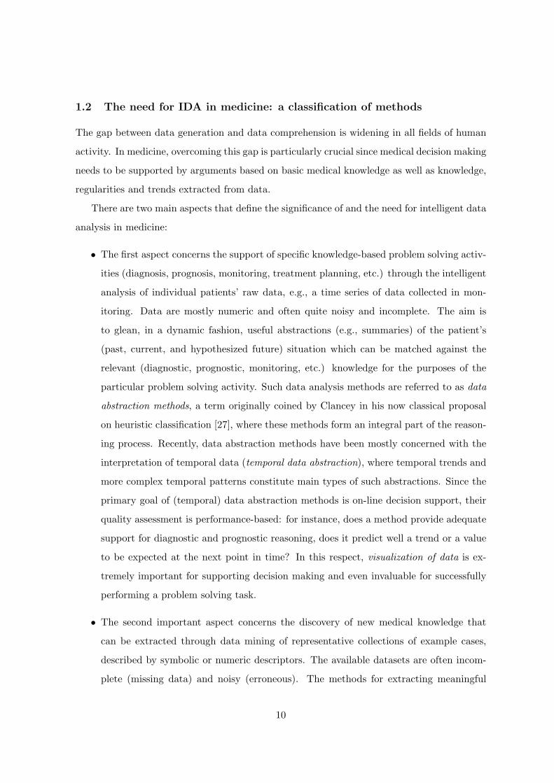
main problems addressed at this early stage of expert system research concerned knowledge
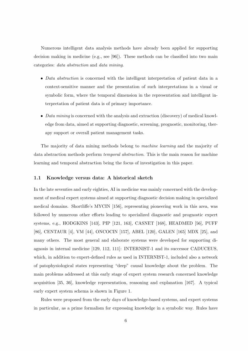
acquisition [35, 36], knowledge representation, reasoning and explanation [167]. A typical
early expert system schema is shown in Figure 1.
Rules were proposed from the early days of knowledge-based systems, and expert systems
in particular, as a prime formalism for expressing knowledge in a symbolic way. Rules have
6
the undisputed advantages of simplicity, uniformity, transparency, and ease of inference, that
over the years have made them one of the most widely adopted approaches for representing
real world knowledge. Rules elicited directly from domain experts are expressed at the right
level of abstraction from the perspective of the expert, and are indeed comprehensible to the
expert since they are formulations of his rules of thumb. However, human-defined rules risk
capturing the biases of one expert, and although each rule individually may appear to form
a coherent, modular chunk of knowledge, the analysis of rules as an integral whole can reveal
inconsistencies, gaps, and various other deficiencies due to their largely flat organization (i.e.,
the lack of a comprehensive, global, hierarchical organization of the rules).
It soon became clear that knowledge acquisition is the hardest part of the expert system
development task. This was identified as the so-called “Feigenbaum bottleneck” [47, 48] in
the construction of a knowledge base. The knowledge base is the heart of an expert system.
For the effective use of expert system technology a knowledge base needs to be consistent and
as complete as possible, throughout its deployment; to attain these desirable characteristics,
both manual knowledge maintenance should be facilitated and the system should be able to
evolve on the basis of its problem solving experience. The limitations of the first generation
of expert systems [72, 95] coupled with the relatively high costs (in human and other terms)
involved in acquiring knowledge directly from the experts, as well as the fact that databases
of example cases started becoming readily available, made the learning of rules from such
data especially appealing as a more efficient, less biased, and more cost-effective approach.
On the one hand, this led to the developments in the area of machine learning as described
below, and on the other hand, to the investigations of the use of deep causal knowledge that
could potentially overcome the difficulties encountered when using unstructured shallow-level
inferenceengine
knowledgebase
userinterface
......................................
......................................
......................................................
................................
................................
....................................................................
.....................................................................................................................................................................................
........
......................................
...................................... ......................................
expert
user
Figure 1: An expert system schema of early ’80s.
7
sets of rules [73, 66]. An early approach to combining the use of deep knowledge and machine
learning was used in the development of KARDIO, a system for ECG diagnosis of cardiac
arrhythmias [16].
In the late eighties and early nineties it became apparent that knowledge acquired from
experts alone is unsuitable for solving difficult problems and that, when developing decision
support systems, the analysis of data gathered in the daily practice of experts and stored
systematically in databases can play an important role in supporting the decision making
process. This led to the development of early machine learning algorithms [106, 132] aimed at
the automatic extraction of rules or decision trees from data. Early machine learning systems,
dealing with real-world data which may be erroneous (noisy) and incomplete, include CART
[18], Quinlan’s extensions to ID3 [133], ASSISTANT [17, 24], AQ [109], and CN2 [29, 28].
The C4.5 system [135] is an efficient and probably the most popular machine learning system
of the nineties.
inferenceengine
knowledgebase
protocols,guidelines,
etc.
datamining
temporalabstraction
visualization
userinterface
......................................
......................................
......................................
......................................................
................................................................................
. . . . . . . . . . . . . . . . . . . . . . . . . . . . . . . . . . . . . . . . . .............................................................
............................................................................................
......................................................
......................................................
..................................................................
.......................
............................................................................................................................................................................................................................................................................................
...
......................................
....................
....................
....................
....................
....................
....................
....................
....................
....................
....................
............
......................................
......................................
..............................
..............................
..............................
..............................
....................................................
............................................................................................................................................
............................................................................................................................................
.................................................................................................................................................................................................................................................................................................................................
......................................
...................................... ......................................
......................................
......................................
......................................
...................................... ......................................
............................................................................
......................................
.......................................................................................................................................................................... ......................................
............................................................................................................................................. ......................................
........................................................................................................................................................................................................................
..............................................................
..............................................................
..............................................................
..............................................................
...............................................................
data collection
IDA, KDD
- textual data- images
electronic patient records
user
intranetInternet
expert
(Internet/intranet)
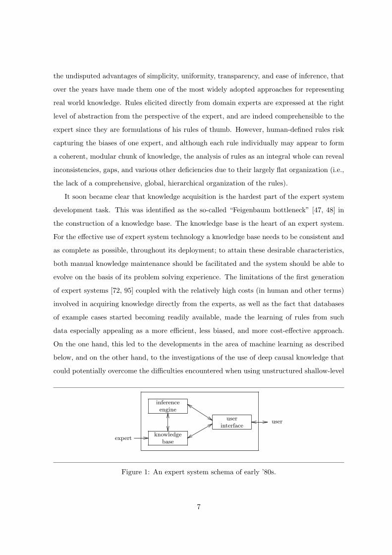
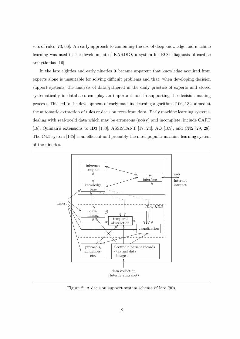
Figure 2: A decision support system schema of late ’90s.
8
Machine learning approaches do not advocate the bypassing of experts. Far from it.
Experts are actively involved, but in a different and more constructive way than in the
development of early expert systems. The example cases come from the experts and the
resulting rules are validated by the experts for comprehensibility and other desired qualities.
The learning approaches ensure that the derived rules are consistent, hierarchically organized
(for example in terms of a decision tree), and, assuming that the collection of case examples
used provides an adequate coverage of the particular domain, the resulting set of rules will
be of sufficient accuracy and adequate coverage (i.e., without significant gaps of knowledge).
Furthermore, the expert provides important background knowledge for focusing and guiding
the learning of rules. Irrespective of whether rules are learned or directly acquired from
experts, their format should be simple, intuitive, and adequately expressive for the purposes
of the particular application.
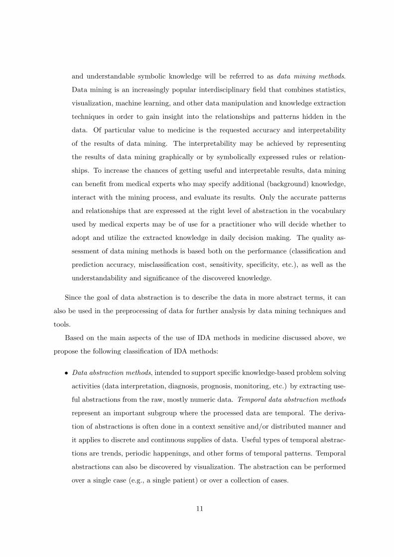
The nineties are characterized by the increasing gap between the massive storage of un-
interpreted data and the understanding of the data, and the need to overcome this gap by
the effective use of data analysis techniques. The main emphasis of current research is thus
on data analysis. This led to the challenging new research areas of knowledge discovery in
databases [51], data mining, and intelligent data analysis, in which machine learning tech-
niques have a major role when the goal of data analysis is knowledge extraction. Current
machine learning research is characterized by a shift of emphasis towards relational learning
(ILP, [116, 93]) and more elaborate statistics applied in learning and evaluation methodolo-
gies. In data analysis, another trend is towards data abstraction and, in particular, towards
temporal data abstraction [67] that can be viewed as a form of preprocessing for further data
analysis. In the late nineties, data analysis has an increased role due to the fact that data
gathering is becoming distributed (e.g., telemedicine [8]), and that the analysis of such data is
even more demanding. Figure 2 shows a possible schema of a decision support system of the
nineties, where decision support needs to deal also with large volumes of data, as well as data
gathering and analysis via the Internet and an intranet (see also [14]). In the figure, arrows
denote the normal information flow, and dotted arrows represent information flow that occurs
in processes which involve iteration and loops between the different steps of the intelligent
data analysis process.
9
1.2 The need for IDA in medicine: a classification of methods
The gap between data generation and data comprehension is widening in all fields of human
activity. In medicine, overcoming this gap is particularly crucial since medical decision making
needs to be supported by arguments based on basic medical knowledge as well as knowledge,
regularities and trends extracted from data.
There are two main aspects that define the significance of and the need for intelligent data
analysis in medicine:
• The first aspect concerns the support of specific knowledge-based problem solving activ-
ities (diagnosis, prognosis, monitoring, treatment planning, etc.) through the intelligent
analysis of individual patients’ raw data, e.g., a time series of data collected in mon-
itoring. Data are mostly numeric and often quite noisy and incomplete. The aim is
to glean, in a dynamic fashion, useful abstractions (e.g., summaries) of the patient’s
(past, current, and hypothesized future) situation which can be matched against the
relevant (diagnostic, prognostic, monitoring, etc.) knowledge for the purposes of the
particular problem solving activity. Such data analysis methods are referred to as data
abstraction methods, a term originally coined by Clancey in his now classical proposal
on heuristic classification [27], where these methods form an integral part of the reason-
ing process. Recently, data abstraction methods have been mostly concerned with the
interpretation of temporal data (temporal data abstraction), where temporal trends and
more complex temporal patterns constitute main types of such abstractions. Since the
primary goal of (temporal) data abstraction methods is on-line decision support, their
quality assessment is performance-based: for instance, does a method provide adequate
support for diagnostic and prognostic reasoning, does it predict well a trend or a value
to be expected at the next point in time? In this respect, visualization of data is ex-
tremely important for supporting decision making and even invaluable for successfully
performing a problem solving task.
• The second important aspect concerns the discovery of new medical knowledge that
can be extracted through data mining of representative collections of example cases,
described by symbolic or numeric descriptors. The available datasets are often incom-
plete (missing data) and noisy (erroneous). The methods for extracting meaningful
10
and understandable symbolic knowledge will be referred to as data mining methods.
Data mining is an increasingly popular interdisciplinary field that combines statistics,
visualization, machine learning, and other data manipulation and knowledge extraction
techniques in order to gain insight into the relationships and patterns hidden in the
data. Of particular value to medicine is the requested accuracy and interpretability
of the results of data mining. The interpretability may be achieved by representing
the results of data mining graphically or by symbolically expressed rules or relation-
ships. To increase the chances of getting useful and interpretable results, data mining
can benefit from medical experts who may specify additional (background) knowledge,
interact with the mining process, and evaluate its results. Only the accurate patterns
and relationships that are expressed at the right level of abstraction in the vocabulary
used by medical experts may be of use for a practitioner who will decide whether to
adopt and utilize the extracted knowledge in daily decision making. The quality as-
sessment of data mining methods is based both on the performance (classification and
prediction accuracy, misclassification cost, sensitivity, specificity, etc.), as well as the
understandability and significance of the discovered knowledge.
Since the goal of data abstraction is to describe the data in more abstract terms, it can
also be used in the preprocessing of data for further analysis by data mining techniques and
tools.
Based on the main aspects of the use of IDA methods in medicine discussed above, we
propose the following classification of IDA methods:
• Data abstraction methods, intended to support specific knowledge-based problem solving
activities (data interpretation, diagnosis, prognosis, monitoring, etc.) by extracting use-
ful abstractions from the raw, mostly numeric data. Temporal data abstraction methods
represent an important subgroup where the processed data are temporal. The deriva-
tion of abstractions is often done in a context sensitive and/or distributed manner and
it applies to discrete and continuous supplies of data. Useful types of temporal abstrac-
tions are trends, periodic happenings, and other forms of temporal patterns. Temporal
abstractions can also be discovered by visualization. The abstraction can be performed
over a single case (e.g., a single patient) or over a collection of cases.
11
• Data mining methods, intended to extract knowledge preferably in a meaningful and
understandable symbolic form. Most frequently applied methods in this context are su-
pervised symbolic machine learning methods. For example, effective tools for inductive
learning exist that can be used to generate understandable diagnostic and prognostic
rules. Symbolic clustering, discovery of concept hierarchies, qualitative model discovery,
and learning of probabilistic causal networks fit in this framework as well. Sub-symbolic
learning and case-based reasoning methods can also be classified in the data mining cat-
egory. Other frequently applied sub-symbolic methods are the nearest neighbor method,
Bayesian classifier, and (non-symbolic) clustering.
2 Data abstraction
Time is intrinsic to many medical problem domains. Disease processes evolve in time, patient
records give the history of patients, and therapeutic actions, like all actions, are indescribable
without considering time. For such domains, time should be explicitly represented in an inte-
gral fashion and reasoned about. The modeling of time enables a more accurate formation of
potential solutions (e.g., the presence of an abnormality may not be diagnostically significant
as such, but its specific pattern of appearance is) and a more accurate evaluation of the en-
tertained solutions (e.g., the expected picture of a disease is different depending on the state
of its evolution).
Abstractions for which time plays a central role are called temporal abstractions. For ex-
ample temporal reasoning is central in establishing the existence of some delay or prematurity
in the unfolding of some ossification process, or the existence of some trend. Temporal data
abstraction is presently attracting considerable research interest [54, 63, 70, 90, 110, 118, 142,
150, 151], as a fundamental intermediate reasoning process for the intelligent interpretation
of temporal data in support of tasks such as diagnosis, monitoring, etc. Background domain
knowledge [74] can be effectively utilized in the context of temporal data abstraction.
2.1 The need for data abstraction in medical problem solving
Medical knowledge-based systems involve the application of medical knowledge on patient
specific data with the goal of reaching some diagnosis or prognosis, deciding the best ther-
12
apy regime for the patient, or monitoring the effectiveness of some ongoing therapy and if
necessary applying rectification actions. Medical knowledge, like any kind of knowledge, is
expressed in a form which is as general as possible, say in terms of associations or rules, causal
models of patophysiological states, behavior (evolution) models of disease processes, patient
management protocols and guidelines, etc. Data on a particular patient, on the other hand,
comprise numeric measurements of various parameters (such as blood pressure, body temper-
ature, etc.) at different points in time. The record of a patient gives the history of the patient
(past operations and other treatments), results of laboratory and physical examinations as
well as the patient’s own symptomatic recollections.
To perform any kind of medical problem solving, patient data have to be “matched”
against medical knowledge. A forward-driven rule is activated if its antecedent can be uni-
fied against patient information, similarly a patient management protocol is activated if its
underlying preconditions can be unified against patient information, etc. The difficulty en-
countered here is that often the abstraction gap between the highly specific, raw patient data,
and the highly abstract medical knowledge does not permit any direct unification between
data and knowledge. The process of data abstraction aims to close this gap, in other words
it aims to bring the raw patient data to the level of medical knowledge in order to permit the
derivation of diagnostic, prognostic or therapeutic conclusions. Hence data abstraction can
be seen as an auxiliary process that aids the problem solving process per se. However it is a
critical auxiliary process since the success of a medical knowledge-based system can depend
on it. Data abstraction involves low level processing, but this processing can be even more
“intelligent” and computationally demanding than the higher level reasoning process itself.
The significance of a data abstraction process in the context of a knowledge-based system
was first perceived by Clancey [27] in his proposal on heuristic classification. In Clancey’s
work data abstraction is used as the stepping stone towards the activation of nodes on a
solution hierarchy. Such nodes, especially at the high levels of the hierarchy, are associated
with triggers, where a trigger is a conjunction of observable items of information. In heuristic
classification, data abstraction is applied in an event-driven fashion with the aim of mapping
raw case data to the level of abstraction used in the expression of triggers, in order to enable
the activation (i.e., their unification against data) of triggers.
Thus needless to say that a knowledge-based system that does not possess any data ab-
13
straction capabilities would require its user to express the case data at the level of abstraction
corresponding to its knowledge. Such a system puts the onus on the user to perform the data
abstraction process. This approach has limitations. Firstly the user, often a non-specialist,
is burdened with the task of not only observing/measuring and reporting data, but also of
interpreting such data for the special needs of the particular problem solving. Secondly, this
is prone to errors and inconsistencies even for domains where it can be considered “doable”,
and it is impossible in domains with large amounts of raw data. In short, the usefulness
of a medical knowledge-based system that does not possess data abstraction capabilities is
substantially reduced.
2.2 Types of data abstraction
The purpose of data abstraction, in the context of medical problem solving, is the intelligent
interpretation of the raw data on some patient, so that the derived abstract data are at the
level of abstraction corresponding to the given body of knowledge. Abstract data are useful
since they can be unified against knowledge; they give the useful abstractions (summaries)
on the patient situation.
There are different types of data abstraction, some are rather simple and others quite
complicated. Due to the rather open-ended nature of data abstraction and the multitude of
ways basic types can be combined to yield complex types, the types discussed below do not
provide an exhaustive classification of all the types of abstractions.
The common feature of all these types, even the very simple ones, is that their derivation
is knowledge-driven; hence data abstraction is itself a knowledge-based process. The use of
knowledge in the derivation of abstractions is the feature that distinguishes data abstrac-
tion from statistical data analysis, e.g., the derivation of trends through time-series analysis.
Data abstraction is knowledge-based and heuristic while statistical analysis is “syntactic” and
algorithmic.
Before listing the types of data abstraction it is necessary to say a few words about the
nature of raw patient data. Their highly specific form has already been stressed. In addition
they can be noisy and inconsistent. For some domains, e.g., intensive care monitoring, the
data are voluminous, while for other domains they are grossly incomplete, e.g., for medical
domains dealing with skeletal abnormalities. Different medical parameters can have very
14
different sampling frequencies and hence different time units (granularities) arise. Thus for
one parameter there could be too much and very specific data, while for another only very
few and far between recordings. In either case, data abstraction tries to determine the useful
(abstract) information, safeguarding against the possibility of noise; in the first case it tries
to eliminate the detail while in the second case to fill the gaps, two orthogonal aims. Since
noise is an unavoidable phenomenon a viable data abstraction process should perform some
kind of data validation and verification which also makes use of knowledge [60].
Simple types of data abstraction are atemporal and often involve a single datum, which
is mapped to a more abstract concept. The knowledge underlying such abstractions often
comprises concept taxonomies or concept associations. Examples of simple data abstractions
are:
• Qualitative abstraction, where a numeric expression is mapped to a qualitative expres-
sion, e.g., “a temperature of 41 degrees C” is abstracted to “fever”. Such abstractions
are based on simple associational knowledge such as <“a temperature of at least 39
degrees C”, “fever”>
• Generalization abstraction, where an instance is mapped to (one of) its class(es), e.g.,
“halothane is administered” is abstracted to “drug is administered”; the concept “halo-
thane” is an instance of the concept class “drug”. Such abstractions are based on (strict
or tangled) concept taxonomies.
• Definitional abstraction, where a datum from one conceptual category is mapped to a
datum in another conceptual category which happens to be its definitional counterpart
in the other context. The movement here is not hierarchical within the same concept
taxonomy, as it is for generalization abstractions, but it is lateral across two different
concept taxonomies. The resulting concept must be more abstract than the originating
concept in some sense, e.g., it refers to something more easily observable. An example of
definitional abstraction is the mapping of “generalized platyspondyly” to “short trunk”.
“Generalized platyspondyly” is a radiological concept, the observation of which requires
the taking of a radiograph of the spine; platyspondyly means flattening of vertebrae
and generalized platyspondyly means the flattening of all vertebrae. “Short trunk” is a
clinical concept, the observation of which does not require any special procedure. The
15
knowledge driving such abstractions consists of simple associations between concepts
across different categories.
In all the above types of data abstraction, time is implicit. The abstractions refer to
the same times, explicitly or implicitly, associated with the raw data. Thus in an atemporal
situation, where everything is assumed to refer to “now”, we have the general implication
holds(P,D) → holds(P, abs(D)), where predicate holds denotes that datum D holds for pa-
tient P now and function abs embodies any of the above types of simple abstraction. Pred-
icate holds can be extended to have a third argument giving an explicit time, thus having
holds(P,D, T ) → holds(P, abs(D), T ). Time is recognized as inherently relevant to medical
problem solving, and hence to medical knowledge and patient data. The record of a patient
can be viewed as a historical database giving information about his past and present, and
even predictions about his future; a more realistic representation is therefore one that con-
siders patient data as temporal objects, where a temporal object is an association between
an item of information and a time. The representation of time with respect to patient data
is point-based, since the sampling is discrete even when a high frequency is involved. Also,
as already mentioned different time granularities are used. When time becomes an explicit
and inherent dimension of patient data, and medical knowledge, it plays a central role in
data abstraction, hence the name temporal data abstraction. The derivation of temporal
abstractions is presently receiving considerable attention [67].
The dimension of time adds a new aspect of complexity to the derivation of (temporal)
abstractions. In the simple types of (atemporal) data abstraction discussed above, often it is
just a single datum which is mapped to a more abstract datum. In temporal abstractions,
however, it is a cluster of (time-stamped) data which is mapped to an abstract temporal
datum. Atemporal data abstraction is “concept abstraction”, going from a specific concept
to a more abstract concept. Temporal data abstraction is both “concept abstraction” and
“temporal abstraction”. The latter encompasses different notions, such as going from discrete
time-points (used in the expression of raw patient data) to continuous (convex) time-intervals
or (nonconvex) collections of time-intervals (used in the expression of medical knowledge), or
moving from a fine time granularity to a coarser time granularity, etc. Temporal data abstrac-
tion can therefore be decomposed into concept abstraction, i.e., atemporal data abstraction,
followed by temporal abstraction. The reverse sequence is not valid since the (concrete)
16
concepts involved have to be mapped to more abstract concepts, to facilitate temporal ab-
stractions.
Temporal data abstraction entails temporal reasoning, both of a commonsense nature
(e.g., intuitive handling of multiple time granularities and temporal relations such as before,
overlaps, disjoint, etc.), as well as of a specialist nature dealing with persistence semantics
of concepts, etc. Examples of important types of temporal abstraction are (a datum in this
context is assumed to be an association between a property and a temporal aspect, which
often is a time-point at a given time-unit; a simple property is a tuple comprising a subject
(parameter or concept) and a list of attribute value pairs):
• Merge abstraction, where a collection of data, sharing the same, concatenable [155],
property and whose temporal aspects collectively form a (possibly overlapping) chain
(at some time granularity) are abstracted to a single datum with the given property
whose temporal aspect is the maximal time-interval spanning the original data. For
example, three consecutive daily recordings of fever, can be mapped to the temporal
abstraction that the patient had fever for a three day interval. Merge abstraction is
also known as state abstraction, since its aim is to derive maximal intervals over which
there is no change in the state of some parameter.
• Persistence abstraction, where again the aim is to derive maximal intervals spanning the
extent of some property; here though there could be just one datum on that property,
and hence the difficulty is in filling the gaps by “seeing” both backwards and forwards
in time from the specific, discrete, recording of the given property. For example, if it is
known that the patient had headache in the morning, can it be assumed that he also had
headache in the afternoon and/or the evening before? Also if the patient is reported to
have gone blind in one eye in December 1997 can it be assumed that this situation per-
sists now? In some temporal reasoning approaches the persistence rule used is that some
property is assumed to persist indefinitely until some event (e.g., a therapy) is known
to have taken place and this terminates the persistence of the property. This rule is
obviously unrealistic for patient data, since often symptoms have a finite existence and
go away even without the administration of any therapy. Thus, persistence derivation
with respect to patient data can be a complicated process, drawing from the persistence
semantics of properties [71]. These categorize properties into finitely or infinitely per-
17
sisting, where finitely persisting properties are further categorized into recurring and
non-recurring. In addition, ranges for the duration (at relevant time granularities) of
finitely persisting properties may be specified, in the absence of any external factors such
as treatments, etc. Thus blindness could be classified as an infinitely persistent prop-
erty, chickenpox as a finitely persisting but not a recurring property, and flu as a finitely
persisting, recurring, property. Persistence derivation is often context-sensitive, where
contexts can also be dynamically derived (abstracted) from the raw data [147, 148].
For example if it is known that the patient with the headache took aspirin at noon,
it can be derived that the persistence of headache lasted up to about 1pm and that
there was no headache up to 3pm. This is based on the derivation of the time interval
spanning the persistence of the effectiveness of the event of aspirin administration; e.g.,
relevant knowledge may dictate that this starts about 1 hour after the occurrence of the
event and lasts for about 2 hours. Such time intervals defining the persistence of the
effectiveness of treatments are referred to as context intervals. Qualitative abstraction
(see above) can also be context-sensitive.
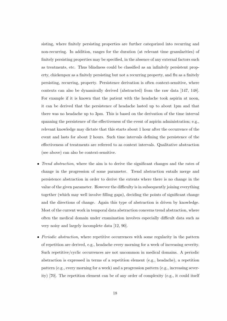
• Trend abstraction, where the aim is to derive the significant changes and the rates of
change in the progression of some parameter. Trend abstraction entails merge and
persistence abstraction in order to derive the extents where there is no change in the
value of the given parameter. However the difficulty is in subsequently joining everything
together (which may well involve filling gaps), deciding the points of significant change
and the directions of change. Again this type of abstraction is driven by knowledge.
Most of the current work in temporal data abstraction concerns trend abstraction, where
often the medical domain under examination involves especially difficult data such as
very noisy and largely incomplete data [12, 90].
• Periodic abstraction, where repetitive occurrences with some regularity in the pattern
of repetition are derived, e.g., headache every morning for a week of increasing severity.
Such repetitive/cyclic occurrences are not uncommon in medical domains. A periodic
abstraction is expressed in terms of a repetition element (e.g., headache), a repetition
pattern (e.g., every morning for a week) and a progression pattern (e.g., increasing sever-
ity) [70]. The repetition element can be of any order of complexity (e.g., it could itself
18
be a periodic abstraction, or a trend abstraction, etc.), giving rise to very complex peri-
odic abstractions. The period spanning the extent of a periodic occurrence is nonconvex
[87, 97] by default, i.e., it is the collection of time intervals spanning the extents of the
distinct instantiations of the repetition element, and hence the collection can include
gaps. Periodic abstraction encompasses the other types of data abstraction and it is
also knowledge driven. Relevant knowledge can include acceptable regularity patterns,
means for justifying local irregularities, etc. The knowledge-intensive, heuristic, deriva-
tion of periodic abstractions is currently largely unexplored although its significance in
medical problem solving is widely acknowledged [61].
The above types of data abstraction can be combined in a multitude of ways yielding
complex abstractions. As already explained, data abstraction is deployed in the context of
some problem solving systems and hence the derivation of abstractions is largely done in a
directed fashion. This means that the given system, in exploring its hypothesis space, predicts
various abstractions which the data abstraction process is required to corroborate against the
raw patient data; in this respect the data abstraction process is goal-driven. However, for the
creation of the initial hypothesis space the data abstraction process needs to operate in a non-
directed or event-driven fashion (as already discussed with respect to Clancey’s proposal). In
the context of a monitoring system, data abstraction, which is the heart of the system, in
fact operates in a largely event-driven fashion. This is because the aim is to comprehensively
interpret all the data covered by the moving time window underlying the operation of the
monitoring system, i.e., to derive all abstractions, of any degree of complexity, and on the
basis of such abstractions the system decides whether the patient situation is static, or it is
improving or worsening.
Non-directed data abstraction repeatedly applies the different types of data abstraction,
until no more derivations are possible. Data abstraction, operating under such a mode, can
be used in a stand alone fashion, i.e., in direct interaction with the user rather than a higher
level reasoning engine; in such a case the derived abstractions should be presented to the user
in a visual form. Visualization is also of relevance when a data abstraction process is not
used in a stand alone fashion; since the overall reasoning of the system depends critically on
the derived abstractions, a good way of justifying this reasoning is the presentation of the
relevant abstractions in a visual form.
19
Another consideration, of relevance to any inference system, is truth maintenance. For
example raw data may well be received out of temporal sequence. Thus abstractions refer-
ring to the present may need to be modified on the basis of old data that has now become
available (view updating [152]), or abstractions referring to the past are revoked by new data
(hindsight [141]).
2.3 Integration of data abstraction into a problem solving system
Data abstraction is a critical auxiliary process. It is deployed in the context of a higher
level problem solving system, it is knowledge-based and it operates under a goal or event
driven fashion or both. The knowledge used by the data abstraction process comprises both
specialist knowledge and so called “world” knowledge, i.e., common-sense knowledge which
is assumed domain and even task independent. The knowledge is organized on the basis of
some ontology that defines the classes of concepts and the types of relations.
In this section we briefly discuss the mode of integration between a problem solving system,
such as a diagnostic system, and a data abstraction process. This can be described as loosely
or tightly coupled and denotes the level of generality, and thus degree of reusability, of the
data abstraction process. Loosely coupled means that the data abstraction process is domain
independent (e.g., it can be integrated with any diagnostic system irrespective of its medical
domain), task independent (e.g., it can be integrated with different reasoning tasks, such as
diagnosis, monitoring, prognosis, etc., within the same medical domain), or both (e.g., it can
be integrated with different reasoning tasks applied to different domains). Tightly coupled,
on the other hand, means that the data abstraction process is an embedded component of the
problem solving system and thus its usability outside that system is limited. Figure 3 shows
a possible coupling of data abstraction with other patient management processes.
So the ideal would be to have a data abstraction process which is both domain and task
independent. Whether this is achievable it remains to be seen, although some significant
steps have been taken in this direction. The looseness or otherwise of coupling between a
data abstraction process and a problem solving system can be decided on the basis of the
following questions:
• Is the ontology underlying the specialist knowledge, domain independent? If yes, by
unplugging the specialist knowledge and incorporating a knowledge acquisition compo-
20
Figure 3: Data abstraction as a loosely coupled process.
nent that functions to fill the given knowledge base with the relevant knowledge from
another domain, we end up having a traditional skeletal system for data abstraction,
applicable to different domains for the same task.
• Is the overall ontology task independent? If yes, we can obtain a skeletal system for
data abstraction, applicable to different tasks within the same domain.
• Is the specialist knowledge task independent? If yes, the data abstraction process is
already applicable to different tasks within the same domain.
• Do generated abstractions constitute final solutions? If yes, the data abstraction process
is strongly coupled to the problem solving system.
In the spirit of the new generation of knowledge engineering methodologies, the objective
should be to form a library of generic data abstraction methods, different mechanisms for
21
the implementation of such methods and underlying knowledge ontologies (e.g., [149, 142].
Below, a representative sample of data abstraction approaches are briefly reviewed.
2.4 Selected data abstraction approaches
In this section, for illustrative purposes, we briefly overview five approaches to temporal data
abstraction. The first four approaches focus on the derivation of trend abstractions, whereas
the fourth is concerned with periodicity abstractions. Detailed accounts of the selected ap-
proaches and their evaluation so far are available in the literature.
2.4.1 Shahar and Musen’s approach
Shahar and Musen [152, 150, 151] have developed a knowledge-based framework for the cre-
ation of abstract, interval concepts from time-stamped clinical data. The framework has
been implemented in the RESUME system under the CLIPS environment, which provides
the necessary truth maintenance. The principles underlying this framework are generality
and reusability where the use of knowledge is emphasized. More specifically the proposers
define the types of knowledge required (structural, classification, temporal semantic, and
temporal dynamic, knowledge) for the identified temporal abstraction functionalities (con-
text formation, contemporaneous abstraction, temporal inference, temporal interpolation,
and temporal pattern-matching). In a specific application of the framework the actual knowl-
edge is organized under various ontologies for parameter-properties, events, contexts, and
dynamic induction relations of context intervals.
The framework supports four types of abstractions: state, gradient, rate and pattern.
Given a historic database, RESUME aims to infer, in a non directed fashion, all derivable
abstractions of any degree of complexity. The process of derivation is repeatedly applied since
by its very nature a historic database is never fixed.
A significant novelty of this approach, is the dynamic derivation of interpretation contexts;
these could be contemporaneous, prospective and retrospective. Interpretation contexts are
induced by events, such as therapeutic actions. Two or more interpretation contexts could
define generalized interpretation contexts; moreover contexts could be nonconvex, if they
are induced on the basis of repetitive events. Abstractions are generated on the basis of
interpretation contexts, thus the interpretation of the patient data is context sensitive. Several
22
concurrent interpretation contexts can be induced, maintained and queried, thus creating
different interpretations for the same set of data points.
In summary, the underlying ontologies, required knowledge, and supported functionalities
have been specified in great detail, and the soundness of the proposal has been demonstrated
through its application to a number of medical domains (therapy for insulin-dependent di-
abetes, protocol-based care of AIDS and of chronic GVHD, and monitoring of children’s
growth) with promising results.
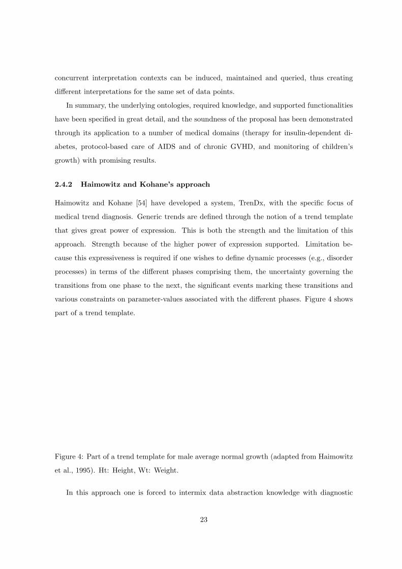
2.4.2 Haimowitz and Kohane’s approach
Haimowitz and Kohane [54] have developed a system, TrenDx, with the specific focus of
medical trend diagnosis. Generic trends are defined through the notion of a trend template
that gives great power of expression. This is both the strength and the limitation of this
approach. Strength because of the higher power of expression supported. Limitation be-
cause this expressiveness is required if one wishes to define dynamic processes (e.g., disorder
processes) in terms of the different phases comprising them, the uncertainty governing the
transitions from one phase to the next, the significant events marking these transitions and
various constraints on parameter-values associated with the different phases. Figure 4 shows
part of a trend template.
Figure 4: Part of a trend template for male average normal growth (adapted from Haimowitz
et al., 1995). Ht: Height, Wt: Weight.
In this approach one is forced to intermix data abstraction knowledge with diagnostic
23
knowledge per se; there is no clear separation between the two, and no diagnostic independent
specification of temporal abstraction knowledge (of the type advocated by Shahar and Musen).
In other words a trend template is a fairly sophisticated mechanism for the specification of
temporal models for dynamic processes, both normal and abnormal processes. There is no
decoupling between an intermediate level of data interpretation (derivation of abstractions)
and a higher level of decision making. Data interpretation involves the selection of the trend
template instantiation that matches best the raw temporal data (this covers noise detection
and positioning of transitions). The selected trend template instantiation is the final solution;
thus temporal data abstraction and diagnostic (or other) reasoning per se are tangled up into
a single process. This makes the overall reasoning more efficient, but it limits the generality
of the approach; the derivation of the abstractions is very much directed (trend template
driven) and hence the potential of this approach as a preprocessing tool for machine learning
is somewhat limited; for the discovery of new knowledge (i.e., new diagnostic rules) the
abstractions used should be derived in a non-directed, i.e., in a non-biased fashion.
TrenDx has been applied, with promising results, to the diagnosis of pediatric growth
disorders and the detection of significant trends in hemodynamics and blood gas in intensive
care unit patients.
2.4.3 Miksch et al. approach
The Miksch et al.’ approach [110], like the one by Haimowitz and Kohane, is aimed at a
specific type of application, and thus unlike the approach by Shahar and Musen, the aim
is not to formulate in generic terms a knowledge-based temporal abstraction task. This
proposal has been realized in VIE-VENT, a system for data validation and therapy planning
for artificially ventilated newborn infants. Like RESUME, VIE-VENT is implemented in the
CLIPS environment.
The overall aim is the context-based validation and interpretation of temporal data, where
data can be of different types (continuously assessed quantitative data, discontinuously as-
sessed quantitative data, and qualitative data). The interpretation contexts are not dynami-
cally derived, but they are defined through schemata with thresholds that can be dynamically
tailored to the patient under examination. The context schemata correspond to potential
treatment regimes; which context is actually active depends on the current regime of the
24
patient. If the interpretation of data points to an alarming situation, the higher level rea-
soning task of therapy assessment and (re)planning is invoked which may result in changing
the patient’s regime thus switching to a new context. Context switching should be done in
a smooth way and again relevant thresholds are dynamically adapted to take care of this.
The data abstraction process per se is fairly decoupled from the therapy planning process.
Hence this approach differs from the previous one where the selection and instantiation of an
interpretation context (trend template) represents the overall reasoning task. In VIE-VENT
the data abstraction process does not need to select the interpretation context, as this is given
to it by the therapy planning process.
The types of knowledge required are classification knowledge and temporal dynamic knowl-
edge (e.g., default persistences, expected qualitative trend descriptions, etc.). Everything is
expressed declaratively in terms of schemata that can be dynamically adjusted depending on
the state of the patient. First quantitative point-based data are translated into qualitative
values, depending on the operative context. Smoothing of data oscillating near thresholds
then takes place. Interval data are then transformed to qualitative descriptions resulting in a
verbal categorization of the change of a parameter over time, using schemata for trend-curve
fitting. The system deals with four types of trends: very short-term, short-term, medium-term
and long-term.
2.4.4 The M-HTP and T-IDDM Systems
M-HTP is a system for monitoring heart-transplant patients that has a module for abstract-
ing time-stamped clinical data [89]. The system relies on two kinds of temporal abstractions,
simple and complex. Simple abstractions are derived from uni-dimensional time series while
complex ones are derived from simple abstractions through Allen’s algebra operators [5] and
can involve different parameters. Example abstractions, called episodes, generated by the
system are “HB-decreasing” or “severe immunodeficiency”. The abstractions are maintained
on a network of temporal intervals. M-HTP uses an object-oriented visit taxonomy and in-
dexes clinical observations by visits. The system has an object-oriented knowledge base that
defines a taxonomy of significant episodes - clinically interesting concepts such as diarrhea or
WBC-decreasing. The M-HTP output includes episodes from the patient temporal network
that can be represented and examined graphically, such as “CMV-viremia-increase”, during
25
particular time periods. The temporal model of M-HTP includes both time points (represent-
ing raw data and visits) and intervals (representing the derived episodes). The system has a
temporal query mechanism, used to evaluate the antecedent part of diagnostic rules, such as
“an episode of decrease in platelet count that overlaps an episode of decrease of WBC count
at least 3 days during the past week implies suspicion of CMV infection”.
The temporal abstraction mechanisms used in M-HTP have been implemented as an
HTTP-based Temporal Abstraction Server (TAS), that has been used for other clinical appli-
cations. In particular, TAS is now used as the basis for the data analysis tools implemented
within the Telematic Management of Insulin Dependent Diabetes Mellitus patient (T-IDDM)
project [13]. In this project, IDDM patients are monitored through an intelligent telemedicine
system, that provides physicians with a collection of distributed services for data storage, anal-
ysis and interpretation, as well as with a rule-based decision support system. The T-IDDM
architecture is now used in clinical practice within the verification and demonstration phase
of the project.
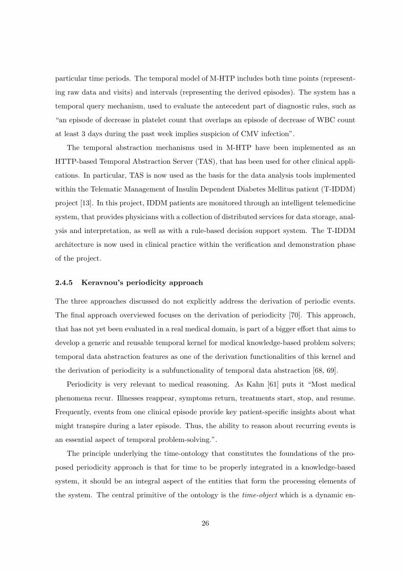
2.4.5 Keravnou’s periodicity approach
The three approaches discussed do not explicitly address the derivation of periodic events.
The final approach overviewed focuses on the derivation of periodicity [70]. This approach,
that has not yet been evaluated in a real medical domain, is part of a bigger effort that aims to
develop a generic and reusable temporal kernel for medical knowledge-based problem solvers;
temporal data abstraction features as one of the derivation functionalities of this kernel and
the derivation of periodicity is a subfunctionality of temporal data abstraction [68, 69].
Periodicity is very relevant to medical reasoning. As Kahn [61] puts it “Most medical
phenomena recur. Illnesses reappear, symptoms return, treatments start, stop, and resume.
Frequently, events from one clinical episode provide key patient-specific insights about what
might transpire during a later episode. Thus, the ability to reason about recurring events is
an essential aspect of temporal problem-solving.”.
The principle underlying the time-ontology that constitutes the foundations of the pro-
posed periodicity approach is that for time to be properly integrated in a knowledge-based
system, it should be an integral aspect of the entities that form the processing elements of
the system. The central primitive of the ontology is the time-object which is a dynamic en-
26
tity, viewed as a tight coupling between a property and an existence. Time-objects can be
compound and can be involved in causal interactions.
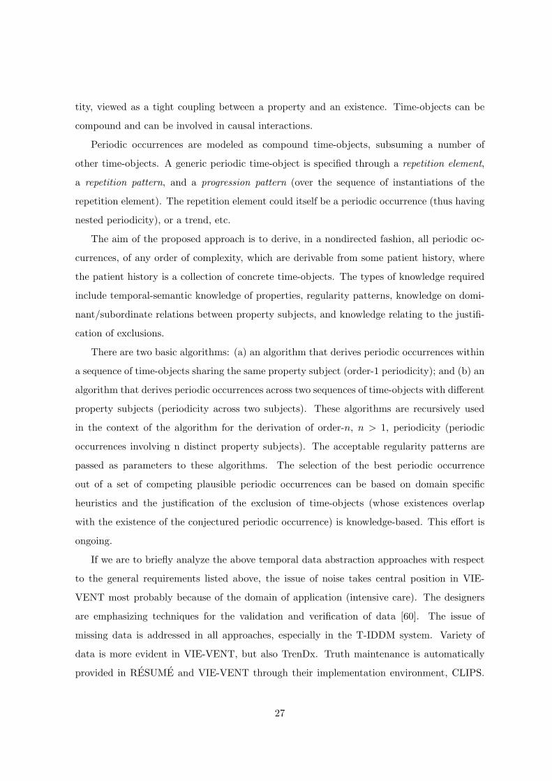
Periodic occurrences are modeled as compound time-objects, subsuming a number of
other time-objects. A generic periodic time-object is specified through a repetition element,
a repetition pattern, and a progression pattern (over the sequence of instantiations of the
repetition element). The repetition element could itself be a periodic occurrence (thus having
nested periodicity), or a trend, etc.
The aim of the proposed approach is to derive, in a nondirected fashion, all periodic oc-
currences, of any order of complexity, which are derivable from some patient history, where
the patient history is a collection of concrete time-objects. The types of knowledge required
include temporal-semantic knowledge of properties, regularity patterns, knowledge on domi-
nant/subordinate relations between property subjects, and knowledge relating to the justifi-
cation of exclusions.
There are two basic algorithms: (a) an algorithm that derives periodic occurrences within
a sequence of time-objects sharing the same property subject (order-1 periodicity); and (b) an
algorithm that derives periodic occurrences across two sequences of time-objects with different
property subjects (periodicity across two subjects). These algorithms are recursively used
in the context of the algorithm for the derivation of order-n, n > 1, periodicity (periodic
occurrences involving n distinct property subjects). The acceptable regularity patterns are
passed as parameters to these algorithms. The selection of the best periodic occurrence
out of a set of competing plausible periodic occurrences can be based on domain specific
heuristics and the justification of the exclusion of time-objects (whose existences overlap
with the existence of the conjectured periodic occurrence) is knowledge-based. This effort is
ongoing.
If we are to briefly analyze the above temporal data abstraction approaches with respect
to the general requirements listed above, the issue of noise takes central position in VIE-
VENT most probably because of the domain of application (intensive care). The designers
are emphasizing techniques for the validation and verification of data [60]. The issue of
missing data is addressed in all approaches, especially in the T-IDDM system. Variety of
data is more evident in VIE-VENT, but also TrenDx. Truth maintenance is automatically
provided in RESUME and VIE-VENT through their implementation environment, CLIPS.
27
Regarding visualization, such work has started in connection with RESUME’s and VIE-
VENT’s abstractions, but this is still at a preliminary state.
Concerning the reusability, the periodicity approach is developed in the context of a generic
temporal kernel and thus reusability is of prime importance. The proposed algorithms are
based on general ontologies and are suitably parameterized with respect to domain specific
heuristics etc. Reusability is the central principle underlying RESUME as well. The various
applications of RESUME so far have demonstrated the reusability potential of the proposed
temporal abstraction methods. VIE-VENT, TrenDx and M-HTP, on the other hand, have
largely focused on the specific needs of their particular application domains, although TrenDx
has been applied to two, quite different, medical domains. Similarly T-IDDM incorporates a
generalization of the temporal abstraction mechanisms used in M-HTP and also emphasizes
the distributed aspect. The issue of reusability is closely related with the mode of integration
between a temporal data abstraction engine and a higher level reasoning engine as explained
in Section 2.3.
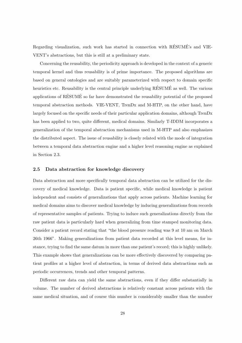
2.5 Data abstraction for knowledge discovery
Data abstraction and more specifically temporal data abstraction can be utilized for the dis-
covery of medical knowledge. Data is patient specific, while medical knowledge is patient
independent and consists of generalizations that apply across patients. Machine learning for
medical domains aims to discover medical knowledge by inducing generalizations from records
of representative samples of patients. Trying to induce such generalizations directly from the
raw patient data is particularly hard when generalizing from time stamped monitoring data.
Consider a patient record stating that “the blood pressure reading was 9 at 10 am on March
26th 1966”. Making generalizations from patient data recorded at this level means, for in-
stance, trying to find the same datum in more than one patient’s record; this is highly unlikely.
This example shows that generalizations can be more effectively discovered by comparing pa-
tient profiles at a higher level of abstraction, in terms of derived data abstractions such as
periodic occurrences, trends and other temporal patterns.
Different raw data can yield the same abstractions, even if they differ substantially in
volume. The number of derived abstractions is relatively constant across patients with the
same medical situation, and of course this number is considerably smaller than the number
28
of raw data. Temporal data abstractions reveal the essence of the profile of a patient, hide
superfluous detail, and last but not least eliminate noisy information. Furthermore, the
temporal scope of abstractions like trends and periodic occurrences are far more meaningful
and prone to adequate comparison than the time-points corresponding to raw data. If the
same complex abstraction, such as a nested periodic occurrence, is associated with a significant
number of patients from a representative sample, it makes a strong candidate for being a
significant piece of knowledge. Sharing a complex abstraction is a strong similarity while
sharing a concrete datum is a weak similarity, if at all.
Current machine learning approaches do not attempt to first abstract, on an individual
basis, the example cases that constitute their training sets, and then to apply whatever
learning technique they employ for the induction of further generalizations. Strictly speaking
every machine learning algorithm performs a kind of abstraction over the entire collection
of cases; however it does not perform any abstraction on the individual cases. Cases tend
to be atemporal, or at best they model time (implicitly) as just another attribute. Data
abstractions on the selected cases are often manually performed by the domain experts as
a preprocessing step. Such manual processing is prone to non-uniformity and inconsistency,
while the automatic extraction of abstractions is uniform and objective.
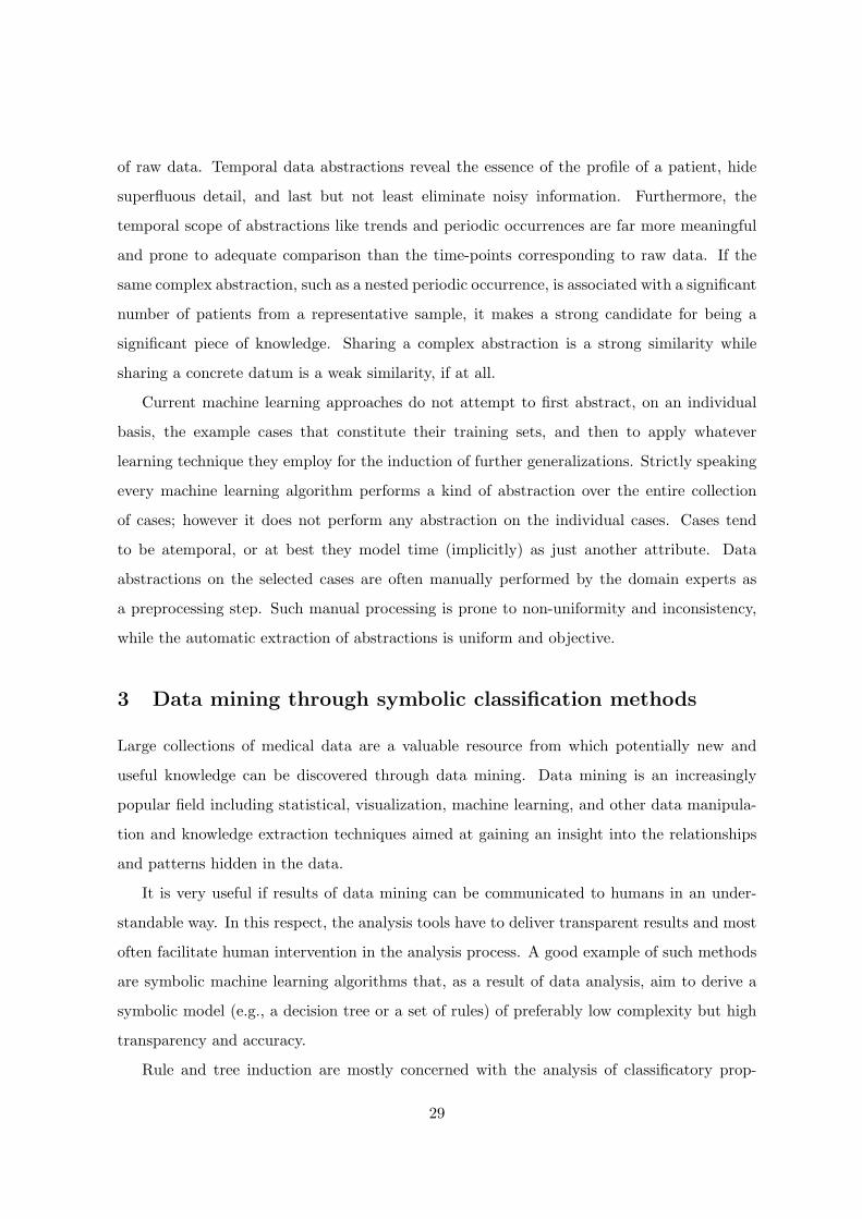
3 Data mining through symbolic classification methods
Large collections of medical data are a valuable resource from which potentially new and
useful knowledge can be discovered through data mining. Data mining is an increasingly
popular field including statistical, visualization, machine learning, and other data manipula-
tion and knowledge extraction techniques aimed at gaining an insight into the relationships
and patterns hidden in the data.
It is very useful if results of data mining can be communicated to humans in an under-
standable way. In this respect, the analysis tools have to deliver transparent results and most
often facilitate human intervention in the analysis process. A good example of such methods
are symbolic machine learning algorithms that, as a result of data analysis, aim to derive a
symbolic model (e.g., a decision tree or a set of rules) of preferably low complexity but high
transparency and accuracy.
Rule and tree induction are mostly concerned with the analysis of classificatory prop-
29
erties of data tables. Data represented in the tables may be collected from measurements
or acquired from experts. Rows in the table correspond to objects (training examples) to
be analyzed in terms of their properties (attributes) and the class (concept) to which they
belong. In a medical setting, a concept of interest could be the set of patients with a certain
disease or outcome. Supervised learning assumes that training examples are classified whereas
unsupervised learning concerns the analysis of unclassified examples.
3.1 Rule induction
3.1.1 If-then rules
Given a set of classified examples, a rule induction system constructs a set of rules. An if-then
rule has the form:
IF Conditions THEN Conclusion.
The condition part of a rule contains one or more attribute tests of the form Ai = vik for
discrete attributes, and Ai < value or Ai > value for continuous attributes. The condition
is a conjunction of attribute tests (or a disjunction of conjunctions of attribute tests). The
conclusion part has the form C = ci, assigning a particular value ci to the class C. An
example is covered by a rule if the attribute values of the example fulfill the conditions in the
IF part of the rule.
An example rule induced in the domain of early diagnosis of rheumatic diseases [92, 42]
is given in Figure 5. It assigns the diagnosis crystal-induced synovitis to male patients older
than 46 who have more than three painful joints and psoriasis as a skin manifestation.
IF Sex = male
AND Age > 46
AND Number_of_painful_joints > 3
AND Skin_manifestations = psoriasis
THEN Diagnosis = Crystal_induced_synovitis
Figure 5: An example if-then rule induced by CN2 in the domain of early diagnosis of
rheumatic diseases.
30
If-then rule induction was studied previously by Michalski [108], and implemented in a
series of AQ algorithms, e.g., the AQ15 system which was also applied for the analysis of
medical data [109].
Here we describe the rule induction system CN2 [29, 28] which is among the best known of
if-then rule learners, capable also of handling imperfect/noisy data. Like the AQ algorithms,
CN2 also uses the covering approach to construct a set of rules for each possible class ci in
turn: when rules for class ci are being constructed, examples of this class are positive, all other
examples are negative. The covering approach works as follows: CN2 constructs a rule that
correctly classifies some examples, removes the positive examples covered by the rule from
the training set and repeats the process until no more examples remain. To construct a single
rule that classifies examples into class ci, CN2 starts with a rule with an empty antecedent
(IF part) and the selected class ci as a consequent (THEN part). The antecedent of this rule
is satisfied by all examples in the training set, and not only those of the selected class. CN2
then progressively refines the antecedent by adding conditions to it, until only examples of
class ci satisfy the antecedent. To allow for the handling imperfect data, CN2 may construct a
set of rules which is imprecise, i.e., does not classify all examples in the training set correctly.
Consider a partially built rule. The conclusion part is already fixed and there are some
(possibly none) conditions in the IF part. The examples covered by this rule form the current
training set. For discrete attributes, all conditions of the form Ai = vik , where vik is a possible
value for Ai, are considered for inclusion in the condition part. For continuous attributes, all
conditions of the form Ai <vik
+vik+1
2 and Ai >vik
+vik+1
2 are considered, where vik and vik+1
are two consecutive values of attribute Ai that actually appear in the current training set.
For example, if the values 4.0, 1.0, and 2.0 for attribute Ai appear in the current training set,
the conditions Ai < 1.5, Ai > 1.5, Ai < 3.0, and Ai > 3.0 will be considered.
Note that both the structure (set of attributes to be included) and the parameters (values
of the attributes for discrete ones and boundaries for the continuous ones) of the rule are
determined by CN2. Which condition will be included in the partially built rule depends on
the number of examples of each class covered by the refined rule and the heuristic estimate
of the quality of the rule.
The heuristic estimates used in rule induction are mainly designed to estimate the perfor-
mance of the rule on unseen examples in terms of classification accuracy. This is in accord
31
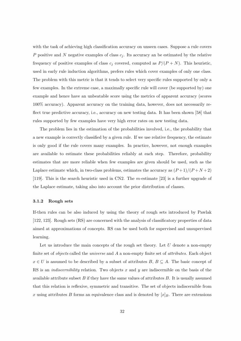
with the task of achieving high classification accuracy on unseen cases. Suppose a rule covers
P positive and N negative examples of class cj . Its accuracy an be estimated by the relative
frequency of positive examples of class cj covered, computed as P/(P + N). This heuristic,
used in early rule induction algorithms, prefers rules which cover examples of only one class.
The problem with this metric is that it tends to select very specific rules supported by only a
few examples. In the extreme case, a maximally specific rule will cover (be supported by) one
example and hence have an unbeatable score using the metrics of apparent accuracy (scores
100% accuracy). Apparent accuracy on the training data, however, does not necessarily re-
flect true predictive accuracy, i.e., accuracy on new testing data. It has been shown [58] that
rules supported by few examples have very high error rates on new testing data.
The problem lies in the estimation of the probabilities involved, i.e., the probability that
a new example is correctly classified by a given rule. If we use relative frequency, the estimate
is only good if the rule covers many examples. In practice, however, not enough examples
are available to estimate these probabilities reliably at each step. Therefore, probability
estimates that are more reliable when few examples are given should be used, such as the
Laplace estimate which, in two-class problems, estimates the accuracy as (P +1)/(P +N +2)
[119]. This is the search heuristic used in CN2. The m-estimate [23] is a further upgrade of
the Laplace estimate, taking also into account the prior distribution of classes.
3.1.2 Rough sets
If-then rules can be also induced by using the theory of rough sets introduced by Pawlak
[122, 123]. Rough sets (RS) are concerned with the analysis of classificatory properties of data
aimed at approximations of concepts. RS can be used both for supervised and unsupervised
learning.
Let us introduce the main concepts of the rough set theory. Let U denote a non-empty
finite set of objects called the universe and A a non-empty finite set of attributes. Each object
x ∈ U is assumed to be described by a subset of attributes B, B ⊆ A. The basic concept of
RS is an indiscernibility relation. Two objects x and y are indiscernible on the basis of the
available attribute subset B if they have the same values of attributes B. It is usually assumed
that this relation is reflexive, symmetric and transitive. The set of objects indiscernible from
x using attributes B forms an equivalence class and is denoted by [x]B. There are extensions
32
of RS theory that do not require transitivity to hold.
Let X ⊆ U , and let IndB(X) denote a set of equivalence classes of examples that are
indiscernible, i.e., a set of subsets of examples that cannot be distinguished on the basis
of attributes in B. The subset of attributes B is sufficient for classification if for every
[x]B ∈ IndB(X) all the examples in [x]B belong to the same decision class. In this case
crisp definitions of classes can be induced; otherwise, only ‘rough’ concept definitions can be
induced since some examples can not be decisively classified.
The main goal of RS analysis is synthesis of approximations of concepts ci. Let X consist
of training examples of class ci. X may be approximated using only the information contained
in B by constructing the B-lower and B-upper approximations of X, denoted BX and BX
respectively, where BX = {x | x ∈ X, [x]B ⊆ X} and BX = {x | x ∈ U, [x]B ∩ X 6= ∅}.
On the basis of the knowledge in B the objects in BX can be classified with certainty as
members of X, while the objects in BX can be only classified as possible members of X.
The set BNB(X) = BX −BX is called the B-boundary region of X thus consisting of those
objects that on the basis of the knowledge in B cannot be unambiguously classified into X
or its complement. The set U −BX is called the B-outside region of X and consists of those
objects which can be with certainty classified as not belonging to X. A set is said to be rough
(respectively crisp) if the boundary region is non-empty (respectively empty). The boundary
region consists of examples that are indiscernible from some examples in X and therefore can
not be decisively classified into ci; this region consists of the union of equivalence classes each
of which contains some examples from X and some examples not in X.
A main task of RS analysis is to find minimal subsets of attributes that preserve the
indiscernibility relation. This is called reduct computation. Note that there are usually
many reducts. Several types of reducts exist. Decision rules are generated from reducts by
reading off the values of the attributes in each reduct. The main challenge in inducing rules
lies in determining which attributes should be included in the conditional part of the rule.
Rules synthesized from the (standard) reducts will usually result in large sets of rules and
are likely to over-fit the patterns of interest. Instead of standard reducts, attribute sets that
“almost” preserve the indiscernibility relation are generated. Good results have been obtained
with dynamic reducts [159] that use a combination of reduct computation and statistical
resampling. Within the RS paradigm new approaches to discretization, feature selection,
33
symbolic attribute grouping, etc. have been designed (for references, see [126, 127, 128]).
There exist several software tools for RS, e.g., the Rosetta system [139].
The list of applications of RS in medicine is significant. It includes extracting diagnostic
rules, image analysis and classification of histological pictures, modeling set residuals, EEG
signal analysis, etc. Examples of RS analysis in medicine include [53, 80, 166]. For an up-to-
date reference that includes medical applications, see [127, 128, 99].
3.1.3 Association rules
The problem of discovering association rules has recently received much attention in the
data mining community. The problem of inducing association rules [2] is defined as follows:
Given a set of transactions, where each transaction is a set of items (i.e., literals of the form
Attribute = value), an association rule is an expression of the form X → Y where X and
Y are sets of items. The intuitive meaning of such a rule is that transactions in a database
which contain X tend to contain Y .
An example of such a rule is: “80% of patients with pneumonia also have high fever. 10%
of all transactions contain both these items.” Here 80% is called confidence of the rule, and
10% support of the rule. Confidence of the rule is calculated as the ratio of the number of
records having true values for all items in X and Y to the number of records having true
values for all items in X. Support of the rule is the ratio of the number of records having true
values for all items in X and Y to the number of all records in the database. The problem is to
find all association rules that satisfy minimum support and minimum confidence constraints.
All association rule learners approach the problem similarly. First all itemsets that satisfy
the minimum support level are generated using different algorithms for traversing the lattice
of subsets. In this way all frequent itemsets are discovered. In the second phase association
rules are constructed from frequent sets without reconsulting the data (which makes the
process efficient): all frequent itemsets are combined with each other to produce all possible
rules satisfying the minimum confidence constraint. If itemsets A and B can be found, such
that A is a proper subset of B and the ratio of frequency of B to frequency of A is above the
specified minimum, then a rule of the form A → C is generated, where C is a set of items in
B but not in A.
Association rule learning was applied in medicine, for example, to identify new and in-
34
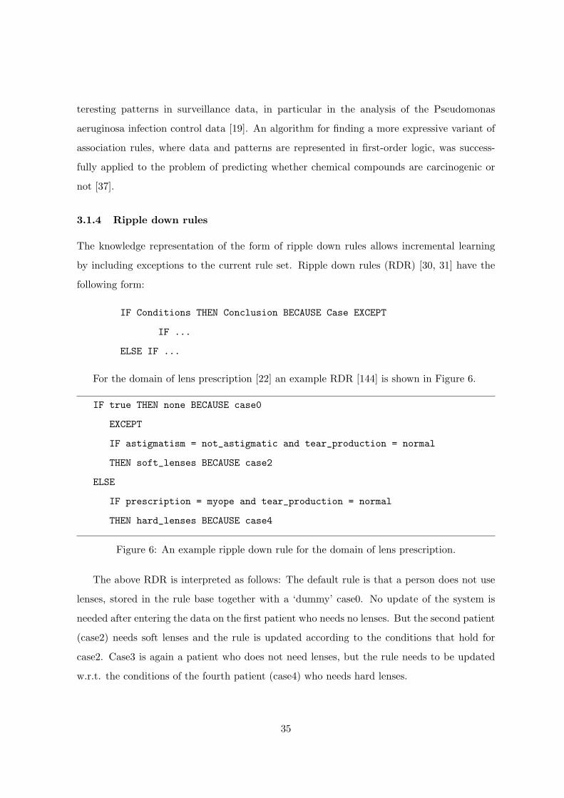
teresting patterns in surveillance data, in particular in the analysis of the Pseudomonas
aeruginosa infection control data [19]. An algorithm for finding a more expressive variant of
association rules, where data and patterns are represented in first-order logic, was success-
fully applied to the problem of predicting whether chemical compounds are carcinogenic or
not [37].
3.1.4 Ripple down rules
The knowledge representation of the form of ripple down rules allows incremental learning
by including exceptions to the current rule set. Ripple down rules (RDR) [30, 31] have the
following form:
IF Conditions THEN Conclusion BECAUSE Case EXCEPT
IF ...
ELSE IF ...
For the domain of lens prescription [22] an example RDR [144] is shown in Figure 6.
IF true THEN none BECAUSE case0
EXCEPT
IF astigmatism = not_astigmatic and tear_production = normal
THEN soft_lenses BECAUSE case2
ELSE
IF prescription = myope and tear_production = normal
THEN hard_lenses BECAUSE case4
Figure 6: An example ripple down rule for the domain of lens prescription.
The above RDR is interpreted as follows: The default rule is that a person does not use
lenses, stored in the rule base together with a ‘dummy’ case0. No update of the system is
needed after entering the data on the first patient who needs no lenses. But the second patient
(case2) needs soft lenses and the rule is updated according to the conditions that hold for
case2. Case3 is again a patient who does not need lenses, but the rule needs to be updated
w.r.t. the conditions of the fourth patient (case4) who needs hard lenses.
35
The above example illustrates also the incremental learning of ripple down rules in which
EXCEPT IF THEN and ELSE IF THEN statements are added to the RDRs to make them con-
sistent with the current database of patients.
If the RDR from Figure 6 were rewritten as an IF-THEN-ELSE statement it would be as
follows:
IF true THEN
IF astigmatism = not_astigmatic and tear_production = normal
THEN soft_lenses ELSE none
ELSE
IF prescription = myope and tear_production = normal
THEN hard_lenses
There have been many successful medical applications of the RDR approach, including
the system PEIRS [43] which is an RDR reconstruction of the hand-built GARVAN expert
system knowledge base on thyroid function tests [59].
3.2 Learning of classification and regression trees
Systems for Top-Down Induction of Decision Trees (TDITD) [133] generate a decision tree
from a given set of attribute-value tuples. Each of the interior nodes of the tree is labeled by
an attribute, while branches that lead from the node are labeled by the values of the attribute.
The tree construction process is heuristically guided by choosing the ‘most informative’
attribute at each step, aimed at minimizing the expected number of tests needed for classifica-
tion. Let E be the current (initially entire) set of training examples, and c1, . . .Nclthe decision
classes. A decision tree is constructed by repeatedly calling a tree construction algorithm in
each generated node of the tree. Tree construction stops when all examples in a node are of
the same class (or if some other stopping criterion is satisfied). This node, called a leaf, is
labeled by a value of the class variable. Otherwise the ‘most informative’ attribute, say Ai,
is selected as the root of the (sub)tree, and the current training set E is split into subsets Ei
according to the values of the most informative attribute. Recursively, a subtree Ti is built
for each Ei.
Ideally, each leaf is labeled by exactly one class name. However, leaves can also be empty,
36
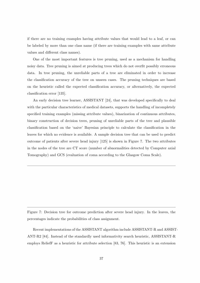
if there are no training examples having attribute values that would lead to a leaf, or can
be labeled by more than one class name (if there are training examples with same attribute
values and different class names).
One of the most important features is tree pruning, used as a mechanism for handling
noisy data. Tree pruning is aimed at producing trees which do not overfit possibly erroneous
data. In tree pruning, the unreliable parts of a tree are eliminated in order to increase
the classification accuracy of the tree on unseen cases. The pruning techniques are based
on the heuristic called the expected classification accuracy, or alternatively, the expected
classification error [135].
An early decision tree learner, ASSISTANT [24], that was developed specifically to deal
with the particular characteristics of medical datasets, supports the handling of incompletely
specified training examples (missing attribute values), binarization of continuous attributes,
binary construction of decision trees, pruning of unreliable parts of the tree and plausible
classification based on the ‘naive’ Bayesian principle to calculate the classification in the
leaves for which no evidence is available. A sample decision tree that can be used to predict
outcome of patients after severe head injury [125] is shown in Figure 7. The two attributes
in the nodes of the tree are CT score (number of abnormalities detected by Computer axial
Tomography) and GCS (evaluation of coma according to the Glasgow Coma Scale).
Figure 7: Decision tree for outcome prediction after severe head injury. In the leaves, the
percentages indicate the probabilities of class assignment.
Recent implementations of the ASSISTANT algorithm include ASSISTANT-R and ASSIST-
ANT-R2 [84]. Instead of the standardly used informativity search heuristic, ASSISTANT-R
employs ReliefF as a heuristic for attribute selection [83, 76]. This heuristic is an extension
37
of RELIEF [75, 76] which is a non-myopic heuristic measure that is able to estimate the
quality of attributes even if there are strong conditional dependencies between attributes.
In addition, wherever appropriate, instead of the relative frequency, ASSISTANT-R uses the
m-estimate of probabilities, which typically improves the performance of machine learning
algorithms [23]. ASSISTANT-R2 is a variant of ASSISTANT-R that, instead of building one
general decision tree for the whole domain, generates one decision tree for each class (diagno-
sis). When classifying a new instance all trees are tried. If several trees classify the instance
into its corresponding class the most probable class is selected. If none of the trees ‘fires’, the
general tree for all the diagnoses generated by ASSISTANT-R is used.
The best known decision tree learner is C4.5 [135] (C5.0 is its recent upgrade) which is
widely used and has also been incorporated into commercial data mining tools (e.g., Clemen-
tine and Kepler). The system is well maintained and documented, reliable, efficient and
capable of dealing with large numbers of training examples. As such, it is considered to be
one of the best data mining tools among those developed by the machine learning community.
Learning of regression trees is similar to decision tree learning: it also uses a top-down
greedy approach to tree construction. The main difference is that decision tree construction
involves the classification into a finite set of discrete classes whereas in regression tree learning
the decision variable is continuous and the leaves of the tree either consist of a prediction into
a numeric value or a linear combination of variables (attributes). An early learning system
CART [18] featured both classification and regression tree learning.
3.3 Inductive logic programming
Inductive logic programming systems learn relational concept descriptions from relational
data. The best known ILP systems include FOIL [134] and Progol [117] and Claudien[38].
LINUS is an environment for inductive logic programming (ILP) [93], enabling learning of
relational descriptions by transforming the training examples and background knowledge into
the form appropriate for attribute-value learners. In general, however, inductive logic pro-
gramming systems learn relational descriptions without such a transformation to propositional
learning.
In ILP, induced rules typically have the form of Prolog clauses. A rule for ocular fundus
image classification for glaucoma diagnosis, as induced by an ILP system GKS [113] specially
38
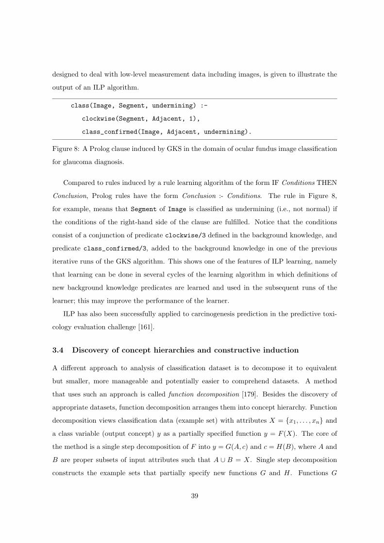
designed to deal with low-level measurement data including images, is given to illustrate the
output of an ILP algorithm.
class(Image, Segment, undermining) :-
clockwise(Segment, Adjacent, 1),
class_confirmed(Image, Adjacent, undermining).
Figure 8: A Prolog clause induced by GKS in the domain of ocular fundus image classification
for glaucoma diagnosis.
Compared to rules induced by a rule learning algorithm of the form IF Conditions THEN
Conclusion, Prolog rules have the form Conclusion :- Conditions. The rule in Figure 8,
for example, means that Segment of Image is classified as undermining (i.e., not normal) if
the conditions of the right-hand side of the clause are fulfilled. Notice that the conditions
consist of a conjunction of predicate clockwise/3 defined in the background knowledge, and
predicate class_confirmed/3, added to the background knowledge in one of the previous
iterative runs of the GKS algorithm. This shows one of the features of ILP learning, namely
that learning can be done in several cycles of the learning algorithm in which definitions of
new background knowledge predicates are learned and used in the subsequent runs of the
learner; this may improve the performance of the learner.
ILP has also been successfully applied to carcinogenesis prediction in the predictive toxi-
cology evaluation challenge [161].
3.4 Discovery of concept hierarchies and constructive induction
A different approach to analysis of classification dataset is to decompose it to equivalent
but smaller, more manageable and potentially easier to comprehend datasets. A method
that uses such an approach is called function decomposition [179]. Besides the discovery of
appropriate datasets, function decomposition arranges them into concept hierarchy. Function
decomposition views classification data (example set) with attributes X = {x1, . . . , xn} and
a class variable (output concept) y as a partially specified function y = F (X). The core of
the method is a single step decomposition of F into y = G(A, c) and c = H(B), where A and
B are proper subsets of input attributes such that A ∪ B = X. Single step decomposition
constructs the example sets that partially specify new functions G and H. Functions G
39
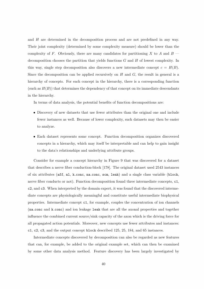
and H are determined in the decomposition process and are not predefined in any way.
Their joint complexity (determined by some complexity measure) should be lower than the
complexity of F . Obviously, there are many candidates for partitioning X to A and B —
decomposition chooses the partition that yields functions G and H of lowest complexity. In
this way, single step decomposition also discovers a new intermediate concept c = H(B).
Since the decomposition can be applied recursively on H and G, the result in general is a
hierarchy of concepts. For each concept in the hierarchy, there is a corresponding function
(such as H(B)) that determines the dependency of that concept on its immediate descendants
in the hierarchy.
In terms of data analysis, the potential benefits of function decompositions are:
• Discovery of new datasets that use fewer attributes than the original one and include
fewer instances as well. Because of lower complexity, such datasets may then be easier
to analyze.
• Each dataset represents some concept. Function decomposition organizes discovered
concepts in a hierarchy, which may itself be interpretable and can help to gain insight
to the data’s relationships and underlying attribute groups.
Consider for example a concept hierarchy in Figure 9 that was discovered for a dataset
that describes a nerve fiber conduction-block [178]. The original dataset used 2543 instances
of six attributes (aff, nl, k conc, na conc, scm, leak) and a single class variable (block,
nerve fiber conducts or not). Function decomposition found three intermediate concepts, c1,
c2, and c3. When interpreted by the domain expert, it was found that the discovered interme-
diate concepts are physiologically meaningful and constitute useful intermediate biophysical
properties. Intermediate concept c1, for example, couples the concentration of ion channels
(na conc and k conc) and ion leakage leak that are all the axonal properties and together
influence the combined current source/sink capacity of the axon which is the driving force for
all propagated action potentials. Moreover, new concepts use fewer attributes and instances:
c1, c2, c3, and the output concept block described 125, 25, 184, and 65 instances.
Intermediate concepts discovered by decomposition can also be regarded as new features
that can, for example, be added to the original example set, which can then be examined
by some other data analysis method. Feature discovery has been largely investigated by
40
Figure 9: Discovered concept hierarchy for the conduction-block domain.
constructive induction, a recently active field within machine learning. The term was first
used by Michalski [108], who defined it as an ability of the system to derive and use new
attributes in the process of learning. Besides pure performance benefits (i.e., in classification
accuracy), constructive induction is useful for data analysis as it may help to induce simpler
and more comprehensible models and to identify interesting inter-attribute relationships. New
attributes may be constructed based on available background knowledge of the domain: an
example of how this facilitated learning of more accurate and comprehensible rules in the
domain of early diagnosis of rheumatic diseases is given in [42]. Function decomposition, on
the other hand, may help to discover attributes from classified instances alone. For the same
rheumatic domain, this was illustrated in [177]. Although such discovery may be carried out
automatically, the benefits of involvement of experts in new attribute selection are typically
significant.
3.5 Case-based reasoning
Case-based reasoning (CBR) uses the knowledge of past experience when dealing with new
cases [1, 100]. A “case” refers to a problem situation — although, as with instance-based
learning [3], cases may be described with a simple attribute-value vector, CBR most often
uses a richer, often hierarchical data structure. CBR relies on a database of past cases that
has to be designed in the way to facilitate the retrieval of similar cases. CBR is a four stage
process:
1. Given a new case to solve, a set of similar cases are retrieved from the database.
41
2. The retrieved cases are reused in order to obtain a solution for a new case. This may
be simply achieved by selecting the most frequent solution used with similar past cases,
or, if an appropriate background knowledge or domain model exists, retrieved solutions
may be adapted for a new case.
3. The solution for the new case is then checked by domain expert, and, if not correct,
repaired using domain-specific knowledge or expert’s input. The specific revision may
be saved and used when solving other new cases.
4. The new case, its solution, and any additional information used for this case that may
be potentially useful when solving new cases are then integrated in the case database.
CBR offers a variety of tools for data analysis. The similar past cases are not just retrieved,
but are also inspected for most relevant features that are similar or different to the case in
question. Because of the hierarchical data organization, CBR may incorporate additional ex-
planation mechanisms. The use of symbolic domain knowledge for solution adaptation may
further reveal specifics and interesting case’s features. When applying CBR to medical data
analysis, however, one has to address several non-trivial questions, including the appropriate-
ness of similarity measures used, the actuality of old cases (the medical knowledge is changing
rapidly), how to handle different solutions (treatment actions) by different physicians, etc.
Several CBR systems were used, adapted for, or implemented to support reasoning and
data analysis in medicine. Some are described in the Special Issue of Artificial Intelligence in
Medicine [101] and include CBR systems for reasoning in cardiology (E. B. Reategui et al.),
learning of plans and goal states in medical diagnosis (B. Lopez and E. Plaza), detection of
coronary heart disease from myocardial scintigrams (M. Haddad et al.), and treatment advice
in nursing (J. Yearwood and R. Wilkinson). Other include a system that uses CBR to assist
in the prognosis of breast cancer [103], case classification in the domain of ultrasonography
and body computed tomography [62], and a CBR-based expert system that advises on the
identification of nursing diagnoses in a new client [15].
4 Data mining through subsymbolic classification methods
In medical problem solving it is important that a decision support system is able to explain
and justify its decisions. Especially when faced with an unexpected solution of a new prob-
42
lem, the user requires substantial justification and explanation. Hence the interpretability
of induced knowledge is an important property of systems that induce solutions from data
about past solved cases. Symbolic data mining methods have this property since they induce
symbolic representations (such as decision trees) from data. On the other hand, subsymbolic
data mining methods typically lack this property which hinders their use in situations for
which explanations are required. Nevertheless, when the classification accuracy is the main
applicability criterion subsymbolic methods may turn out to be very appropriate since they
typically achieve accuracies that are at least as good as those of symbolic classifiers.
4.1 Instance-based learning
Instance-based learning (IBL) algorithms [3] use specific instances to perform classification
tasks, rather than generalizations such as induced if-then rules. IBL algorithms are also
called lazy learning algorithms, as they simply save some or all of the training examples and
postpone all effort towards inductive generalization until classification time. They assume
that similar instances have similar classifications: novel instances are classified according to
the classifications of their most similar neighbors.
IBL algorithms are derived from the nearest neighbor pattern classifier [50, 32]. The
nearest neighbor (NN) algorithm is one of the best known classification algorithms and an
enormous body of research exists on the subject [34]. In essence, the NN algorithm treats
attributes as dimensions of an Euclidean space and examples as points in this space. In the
training phase, the classified examples are stored without any processing. When classifying
a new example, the Euclidean distance between that example and all training examples is
calculated and the class of the closest training example is assigned to the new example.
The more general k-NN method takes the k nearest training examples and determines the
class of the new example by majority vote. In improved versions of k-NN, the votes of each
of the k nearest neighbors are weighted by the respective proximity to the new example [40].
An optimal value of k may be determined automatically from the training set by using leave-
one-out cross-validation [169]. In our experiments in early diagnosis of rheumatic diseases
[42], using the k-NN algorithm implemented by Wettschereck [170], the best k from the range
[1,75] was chosen in this manner. This implementation also incorporates feature weights
determined from the training set. Namely, the contribution of each attribute to the distance
43
may be weighted, in order to avoid problems caused by irrelevant features [171].
Let n = Nat. Given two examples x = (x1, . . . , xn) and y = (y1, . . . , yn), the distance
between them is calculated as
distance(x, y) =
√√√√ n∑i=1
wi × difference(xi, yi)2 (1)
where wi is a non-negative weight value assigned to feature (attribute) Ai and the difference
between attribute values is defined as follows
difference(xi, yi) =
|xi − yi| if Ai is continuous
0 if Ai is discrete and xi = yi
1 otherwise
(2)
When classifying a new instance z, k-NN selects the set K of k-nearest neighbors according
to the distance defined above. The vote of each of the k nearest neighbors is weighted by its
proximity (inverse distance) to the new example. The probability p(z, cj ,K) that instance z
belongs to class cj is estimated as
p(z, cj ,K) =∑
x∈K xcj/distance(z, x)∑x∈K 1/distance(z, x)
(3)
where x is one of the k nearest neighbors of z and xcj is 1 if x belongs to class cj . The class
cj with largest value of p(z, cj ,K) is assigned to the unseen example z.
Before training (respectively before classification), the continuous features are normalized
by subtracting the mean and dividing by the standard deviation so as to ensure that the
values output by the difference function are in the range [0,1]. All features have then equal
maximum and minimum potential effect on distance computations. However, this bias hand-
icaps k-NN as it allows redundant, irrelevant, interacting or noisy features to have as much
effect on distance computation as other features, thus causing k-NN to perform poorly. This
observation has motivated the creation of many methods for computing feature weights.
The purpose of a feature weight mechanism is to give low weight to features that provide no
information for classification (e.g., very noisy or irrelevant features), and to give high weight
to features that provide reliable information. In the k-NN implementation of Wettschereck
44
[170], feature Ai is weighted according to the mutual information [153] I(cj , Ai) between the
class cj and attribute Ai.
4.2 Neural networks
Artificial neural networks may be used for both supervised and unsupervised learning. For
each learning type, we here briefly describe the most frequently used approaches only.
4.2.1 Supervised learning
For supervised learning and among different neural network paradigm, feed-forward multi-
layered neural networks [140, 45] are most frequently used for modeling medical data. They
are computational structures consisting of a interconnected processing elements (PE) or nodes
arranged on a multilayered hierarchical architecture. In general, PE computes the weighted
sum of its inputs and filters it through some sigmoid function to obtain the output (Fig-
ure 10.a). Outputs of PEs of one layer serve as inputs to PEs of the next layer (Figure 10.b).
To obtain the output value for selected instance, its attribute values are stored in input nodes
of the network (the network’s lowest layer). Next, in each step, the outputs of the higher-level
processing elements are computed (hence the name feed-forward), until the result is obtained
and stored in PEs at the output layer.
Figure 10: Processing element (a) and an example of the typical structure of the feed-forward
multi-layered neural network with four processing elements at hidden layer and one at output
layer (b).
A typical architecture of multi-layered neural network comprising an input, hidden, and
output layer of nodes is given in Figure 10.b. The number of nodes in the input and output
45
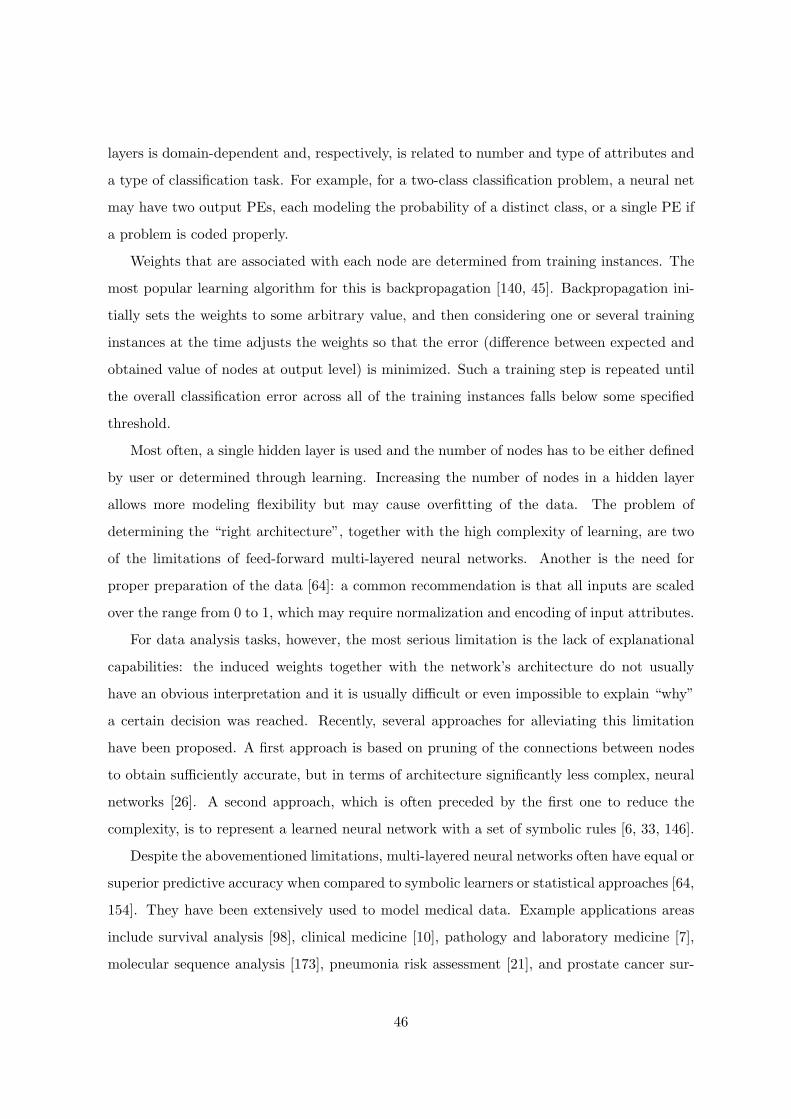
layers is domain-dependent and, respectively, is related to number and type of attributes and
a type of classification task. For example, for a two-class classification problem, a neural net
may have two output PEs, each modeling the probability of a distinct class, or a single PE if
a problem is coded properly.
Weights that are associated with each node are determined from training instances. The
most popular learning algorithm for this is backpropagation [140, 45]. Backpropagation ini-
tially sets the weights to some arbitrary value, and then considering one or several training
instances at the time adjusts the weights so that the error (difference between expected and
obtained value of nodes at output level) is minimized. Such a training step is repeated until
the overall classification error across all of the training instances falls below some specified
threshold.
Most often, a single hidden layer is used and the number of nodes has to be either defined
by user or determined through learning. Increasing the number of nodes in a hidden layer
allows more modeling flexibility but may cause overfitting of the data. The problem of
determining the “right architecture”, together with the high complexity of learning, are two
of the limitations of feed-forward multi-layered neural networks. Another is the need for
proper preparation of the data [64]: a common recommendation is that all inputs are scaled
over the range from 0 to 1, which may require normalization and encoding of input attributes.
For data analysis tasks, however, the most serious limitation is the lack of explanational
capabilities: the induced weights together with the network’s architecture do not usually
have an obvious interpretation and it is usually difficult or even impossible to explain “why”
a certain decision was reached. Recently, several approaches for alleviating this limitation
have been proposed. A first approach is based on pruning of the connections between nodes
to obtain sufficiently accurate, but in terms of architecture significantly less complex, neural
networks [26]. A second approach, which is often preceded by the first one to reduce the
complexity, is to represent a learned neural network with a set of symbolic rules [6, 33, 146].
Despite the abovementioned limitations, multi-layered neural networks often have equal or
superior predictive accuracy when compared to symbolic learners or statistical approaches [64,
154]. They have been extensively used to model medical data. Example applications areas
include survival analysis [98], clinical medicine [10], pathology and laboratory medicine [7],
molecular sequence analysis [173], pneumonia risk assessment [21], and prostate cancer sur-
46
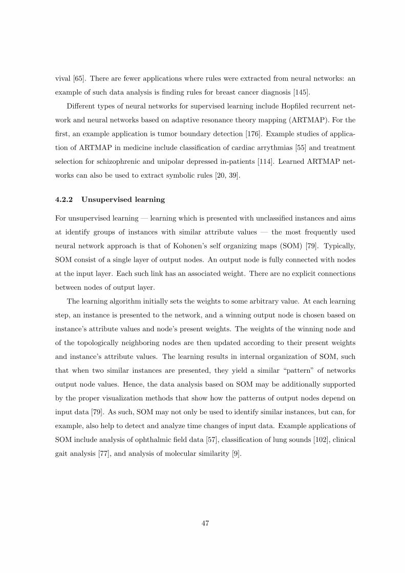
vival [65]. There are fewer applications where rules were extracted from neural networks: an
example of such data analysis is finding rules for breast cancer diagnosis [145].
Different types of neural networks for supervised learning include Hopfiled recurrent net-
work and neural networks based on adaptive resonance theory mapping (ARTMAP). For the
first, an example application is tumor boundary detection [176]. Example studies of applica-
tion of ARTMAP in medicine include classification of cardiac arrythmias [55] and treatment
selection for schizophrenic and unipolar depressed in-patients [114]. Learned ARTMAP net-
works can also be used to extract symbolic rules [20, 39].
4.2.2 Unsupervised learning
For unsupervised learning — learning which is presented with unclassified instances and aims
at identify groups of instances with similar attribute values — the most frequently used
neural network approach is that of Kohonen’s self organizing maps (SOM) [79]. Typically,
SOM consist of a single layer of output nodes. An output node is fully connected with nodes
at the input layer. Each such link has an associated weight. There are no explicit connections
between nodes of output layer.
The learning algorithm initially sets the weights to some arbitrary value. At each learning
step, an instance is presented to the network, and a winning output node is chosen based on
instance’s attribute values and node’s present weights. The weights of the winning node and
of the topologically neighboring nodes are then updated according to their present weights
and instance’s attribute values. The learning results in internal organization of SOM, such
that when two similar instances are presented, they yield a similar “pattern” of networks
output node values. Hence, the data analysis based on SOM may be additionally supported
by the proper visualization methods that show how the patterns of output nodes depend on
input data [79]. As such, SOM may not only be used to identify similar instances, but can, for
example, also help to detect and analyze time changes of input data. Example applications of
SOM include analysis of ophthalmic field data [57], classification of lung sounds [102], clinical
gait analysis [77], and analysis of molecular similarity [9].
47
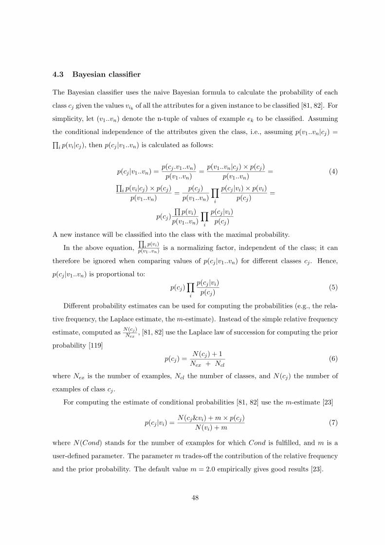
4.3 Bayesian classifier
The Bayesian classifier uses the naive Bayesian formula to calculate the probability of each
class cj given the values vik of all the attributes for a given instance to be classified [81, 82]. For
simplicity, let (v1..vn) denote the n-tuple of values of example ek to be classified. Assuming
the conditional independence of the attributes given the class, i.e., assuming p(v1..vn|cj) =∏i p(vi|cj), then p(cj |v1..vn) is calculated as follows:
p(cj |v1..vn) =p(cj .v1..vn)p(v1..vn)
=p(v1..vn|cj)× p(cj)
p(v1..vn)= (4)∏
i p(vi|cj)× p(cj)p(v1..vn)
=p(cj)
p(v1..vn)
∏i
p(cj |vi)× p(vi)p(cj)
=
p(cj)∏
p(vi)p(v1..vn)
∏i
p(cj |vi)p(cj)
A new instance will be classified into the class with the maximal probability.
In the above equation,∏
ip(vi)
p(v1..vn) is a normalizing factor, independent of the class; it can
therefore be ignored when comparing values of p(cj |v1..vn) for different classes cj . Hence,
p(cj |v1..vn) is proportional to:
p(cj)∏i
p(cj |vi)p(cj)
(5)
Different probability estimates can be used for computing the probabilities (e.g., the rela-
tive frequency, the Laplace estimate, the m-estimate). Instead of the simple relative frequency
estimate, computed as N(cj)Nex
, [81, 82] use the Laplace law of succession for computing the prior
probability [119]
p(cj) =N(cj) + 1
Nex + Ncl(6)
where Nex is the number of examples, Ncl the number of classes, and N(cj) the number of
examples of class cj .
For computing the estimate of conditional probabilities [81, 82] use the m-estimate [23]
p(cj |vi) =N(cj&vi) + m× p(cj)
N(vi) + m(7)
where N(Cond) stands for the number of examples for which Cond is fulfilled, and m is a
user-defined parameter. The parameter m trades-off the contribution of the relative frequency
and the prior probability. The default value m = 2.0 empirically gives good results [23].
48
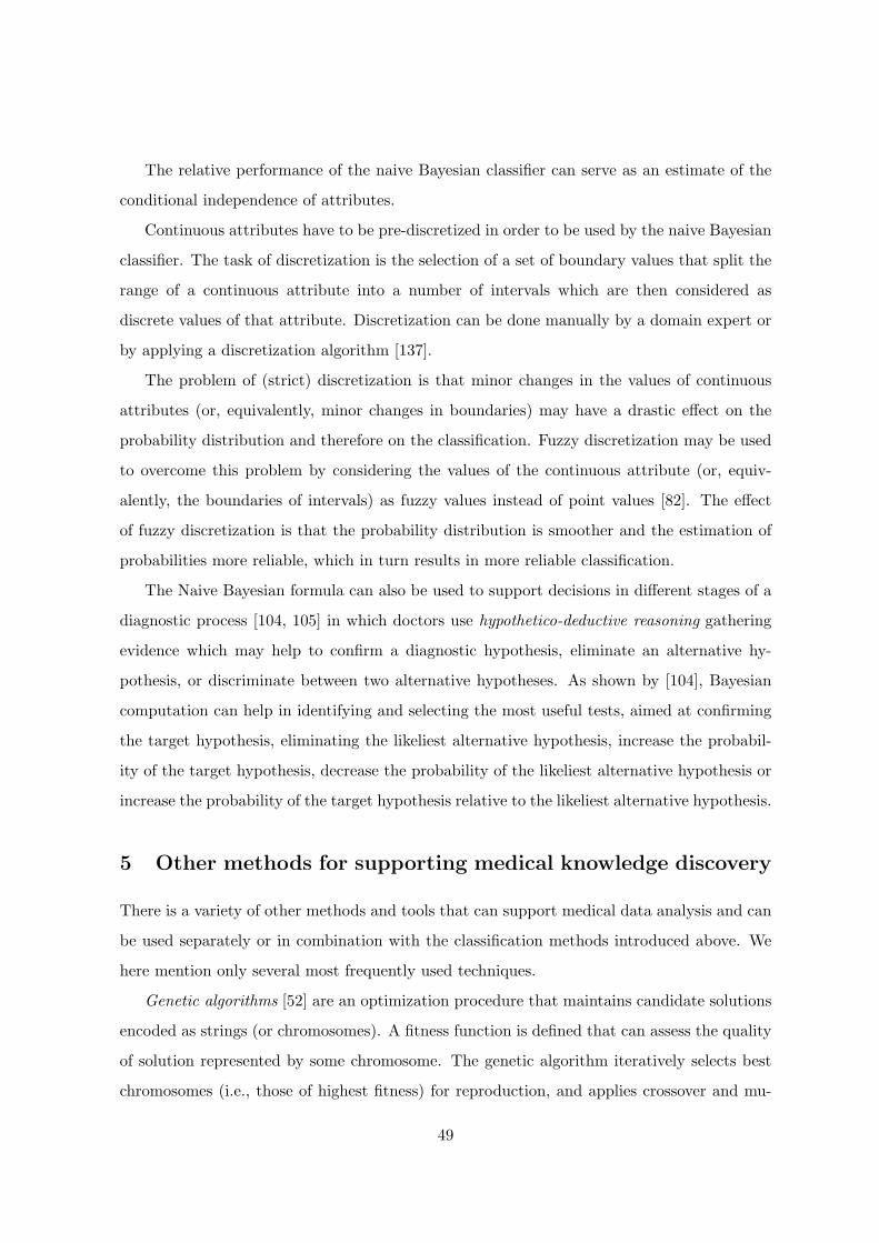
The relative performance of the naive Bayesian classifier can serve as an estimate of the
conditional independence of attributes.
Continuous attributes have to be pre-discretized in order to be used by the naive Bayesian
classifier. The task of discretization is the selection of a set of boundary values that split the
range of a continuous attribute into a number of intervals which are then considered as
discrete values of that attribute. Discretization can be done manually by a domain expert or
by applying a discretization algorithm [137].
The problem of (strict) discretization is that minor changes in the values of continuous
attributes (or, equivalently, minor changes in boundaries) may have a drastic effect on the
probability distribution and therefore on the classification. Fuzzy discretization may be used
to overcome this problem by considering the values of the continuous attribute (or, equiv-
alently, the boundaries of intervals) as fuzzy values instead of point values [82]. The effect
of fuzzy discretization is that the probability distribution is smoother and the estimation of
probabilities more reliable, which in turn results in more reliable classification.
The Naive Bayesian formula can also be used to support decisions in different stages of a
diagnostic process [104, 105] in which doctors use hypothetico-deductive reasoning gathering
evidence which may help to confirm a diagnostic hypothesis, eliminate an alternative hy-
pothesis, or discriminate between two alternative hypotheses. As shown by [104], Bayesian
computation can help in identifying and selecting the most useful tests, aimed at confirming
the target hypothesis, eliminating the likeliest alternative hypothesis, increase the probabil-
ity of the target hypothesis, decrease the probability of the likeliest alternative hypothesis or
increase the probability of the target hypothesis relative to the likeliest alternative hypothesis.
5 Other methods for supporting medical knowledge discovery
There is a variety of other methods and tools that can support medical data analysis and can
be used separately or in combination with the classification methods introduced above. We
here mention only several most frequently used techniques.
Genetic algorithms [52] are an optimization procedure that maintains candidate solutions
encoded as strings (or chromosomes). A fitness function is defined that can assess the quality
of solution represented by some chromosome. The genetic algorithm iteratively selects best
chromosomes (i.e., those of highest fitness) for reproduction, and applies crossover and mu-
49
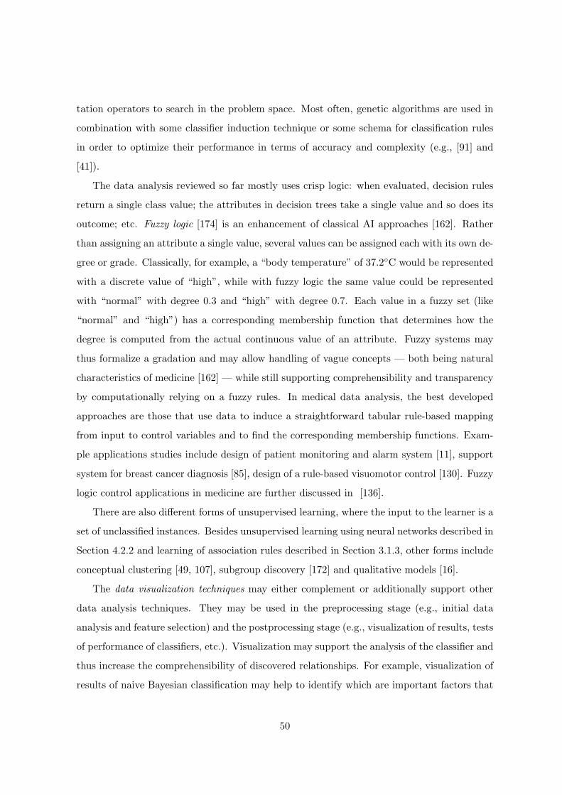
tation operators to search in the problem space. Most often, genetic algorithms are used in
combination with some classifier induction technique or some schema for classification rules
in order to optimize their performance in terms of accuracy and complexity (e.g., [91] and
[41]).
The data analysis reviewed so far mostly uses crisp logic: when evaluated, decision rules
return a single class value; the attributes in decision trees take a single value and so does its
outcome; etc. Fuzzy logic [174] is an enhancement of classical AI approaches [162]. Rather
than assigning an attribute a single value, several values can be assigned each with its own de-
gree or grade. Classically, for example, a “body temperature” of 37.2◦C would be represented
with a discrete value of “high”, while with fuzzy logic the same value could be represented
with “normal” with degree 0.3 and “high” with degree 0.7. Each value in a fuzzy set (like
“normal” and “high”) has a corresponding membership function that determines how the
degree is computed from the actual continuous value of an attribute. Fuzzy systems may
thus formalize a gradation and may allow handling of vague concepts — both being natural
characteristics of medicine [162] — while still supporting comprehensibility and transparency
by computationally relying on a fuzzy rules. In medical data analysis, the best developed
approaches are those that use data to induce a straightforward tabular rule-based mapping
from input to control variables and to find the corresponding membership functions. Exam-
ple applications studies include design of patient monitoring and alarm system [11], support
system for breast cancer diagnosis [85], design of a rule-based visuomotor control [130]. Fuzzy
logic control applications in medicine are further discussed in [136].
There are also different forms of unsupervised learning, where the input to the learner is a
set of unclassified instances. Besides unsupervised learning using neural networks described in
Section 4.2.2 and learning of association rules described in Section 3.1.3, other forms include
conceptual clustering [49, 107], subgroup discovery [172] and qualitative models [16].
The data visualization techniques may either complement or additionally support other
data analysis techniques. They may be used in the preprocessing stage (e.g., initial data
analysis and feature selection) and the postprocessing stage (e.g., visualization of results, tests
of performance of classifiers, etc.). Visualization may support the analysis of the classifier and
thus increase the comprehensibility of discovered relationships. For example, visualization of
results of naive Bayesian classification may help to identify which are important factors that
50
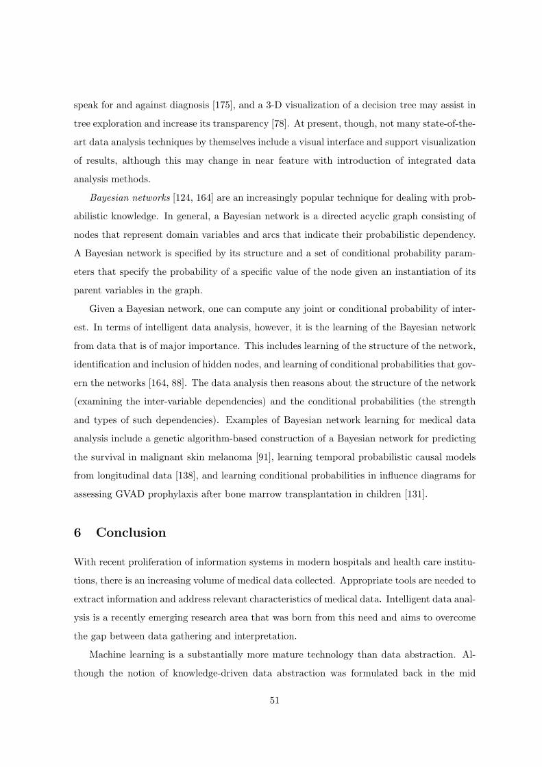
speak for and against diagnosis [175], and a 3-D visualization of a decision tree may assist in
tree exploration and increase its transparency [78]. At present, though, not many state-of-the-
art data analysis techniques by themselves include a visual interface and support visualization
of results, although this may change in near feature with introduction of integrated data
analysis methods.
Bayesian networks [124, 164] are an increasingly popular technique for dealing with prob-
abilistic knowledge. In general, a Bayesian network is a directed acyclic graph consisting of
nodes that represent domain variables and arcs that indicate their probabilistic dependency.
A Bayesian network is specified by its structure and a set of conditional probability param-
eters that specify the probability of a specific value of the node given an instantiation of its
parent variables in the graph.
Given a Bayesian network, one can compute any joint or conditional probability of inter-
est. In terms of intelligent data analysis, however, it is the learning of the Bayesian network
from data that is of major importance. This includes learning of the structure of the network,
identification and inclusion of hidden nodes, and learning of conditional probabilities that gov-
ern the networks [164, 88]. The data analysis then reasons about the structure of the network
(examining the inter-variable dependencies) and the conditional probabilities (the strength
and types of such dependencies). Examples of Bayesian network learning for medical data
analysis include a genetic algorithm-based construction of a Bayesian network for predicting
the survival in malignant skin melanoma [91], learning temporal probabilistic causal models
from longitudinal data [138], and learning conditional probabilities in influence diagrams for
assessing GVAD prophylaxis after bone marrow transplantation in children [131].
6 Conclusion
With recent proliferation of information systems in modern hospitals and health care institu-
tions, there is an increasing volume of medical data collected. Appropriate tools are needed to
extract information and address relevant characteristics of medical data. Intelligent data anal-
ysis is a recently emerging research area that was born from this need and aims to overcome
the gap between data gathering and interpretation.
Machine learning is a substantially more mature technology than data abstraction. Al-
though the notion of knowledge-driven data abstraction was formulated back in the mid
51
eighties, active research in this area is less than ten years old (e.g., [63] represents one of the
early attempts), triggered by research in temporal reasoning in medicine in general [67]. Thus
the interest centers on temporal data abstractions.
So far the two technologies are progressing independently of each other, although they both
have the common objective of analyzing patient data in an intelligent way, but for different
purposes; machine learning for discovering knowledge, and data abstraction for generating
more useful information about a single patient. A research direction worth exploring is the
use of data abstraction in the context of machine learning as suggested above.
Data abstraction as a technology needs to mature further. The emphasis so far has been
on the derivation of temporal trends. This work should continue but should also be expanded
to deal with other types of abstraction such as periodic abstractions. Since the amounts of
raw data involved are often large, computational efficiency, especially for those systems that
need to operate in real time, should be a major concern.
Traditionally, data analysis was the final phase of experimental design that, typically,
included a careful selection of patients, their features and the hypothesis to test. With the
introduction of data warehouses, such a selective approach to data collection is altered and
data may be gathered with no specific purpose in mind. Yet, medical data stored in ware-
houses may provide a useful resource for potential discovery of new knowledge. Researchers
in intelligent data analysis should provide tools for both ends of this spectrum; the proof of
the quality of such tools will be their utility in medical institutions and their acceptability by
the medical experts.
Acknowledgments
This work was supported by research grants of the Ministry of Science and Technology of
Slovenia and the University of Cyprus. Thanks to Riccardo Bellazzi, Peter Flach, Peter
Hammond, Jan Komorowski, Ramon M. Lopez, Silvia Miksch, Enric Plaza and Claude Sam-
mut for their comments on the individual parts of this paper.
References
[1] Aamodt, A., Plaza, E., “Case-based reasoning: Foundational issues, methodological variations, andsystem approaches,” AI Communications, 7(1) 39–59 (1994).
52
[2] Agrawal, R., Manilla, H., Srikant, R., Toivonen, H. and Verkamo A.I., “Fast discovery of associationrules.” In: Advances in Knowledge Discovery and Data Mining (Fayyad, U.M., Piatetsky-Shapiro, G.,Smyth, P. and Uthurusamy, R., eds.), AAAI Press, 1996, pp. 307–328.
[3] Aha, D., Kibler, D., Albert, M., “Instance-based learning algorithms,” Machine Learning, 6: 37–66(1991).
[4] Aikins, J.S., “Prototypes and production rules: An approach to knowledge representation for hypothesisformation.” In: Proc. Sixth International Joint Conference on Artificial Intelligence, 1997, pp. 1–3.
[5] Allen, J.F., “Towards a general theory of action and time,” Artificial Intelligence, 23: 123–154 (1984).
[6] Andrews, R., Diederich, J. and Tickle, A.B., “A survey and critique of techniques for extracting rulesfrom trained artificial neural networks,” Knowledge Based Systems, 8(6): 373–389 (1995).
[7] Astion, M.L. and Wielding, P., “The application of backpropagation neural networks to problems inpathology and laboratory medicine,” Arch Pathol Lab Med, 116: 995–1001 (1992).
[8] Barahona, P. and Christensen, J.P., eds., Knowledge and Decisions in Health Telematics, IOS Press,1994.
[9] Barlow, T.W., “Self-organizing maps and molecular similarity,” Journal of Molecular Graphics, 13(1):53–55 (1995).
[10] Baxt, W.G. “Application of artificial neural networks to clinical medicine,” Lancet, 364(8983) 1135–1138(1995).
[11] Becker, K., Thull, B., Kasmacher-Leidinger, H., Stemmer, J., Rau, G., Kalff, G. and Zimmermann, H.J.“Design and validation of an intelligent patient monitoring and alarm system based on a fuzzy logicprocess model,” Artificial Intelligence in Medicine, 11(1) 33–54 (1997).
[12] Bellazzi, R., Larizza, C. and Riva, A., “Temporal abstractions for pre-processing and interpretingdiabetes monitoring time abstractions.” In Proc. IJCAI-97 Workshop on Intelligent Data Analysis inMedicine and Pharmacology (IDAMAP-97), 1997, pp. 1-9.
[13] Bellazzi, R., Larizza, C., and Riva, A., “Temporal abstractions for interpreting chronic patients moni-toring data,” Intelligent Data Analysis - an International Journal, http://www.elsevier.com/locate/ida,2(2) (1998).
[14] van Bemmel, J.H., “Medical informatics, art or science?” Meth. Inform. Med., 35:157–172 (1996).
[15] Bradburn, C., Zeleznikow, J. and Adams, A., “Florence: synthesis of case-based and model-basedreasoning in a nursing care planning system,” Computers in Nursing, 11(1): 20–24 (1993).
[16] Bratko, I., Mozetic, I. and Lavrac, N., KARDIO: A Study in Deep and Qualitative Knowledge for ExpertSystems, The MIT Press, 1989.
[17] Bratko, I., and Kononenko, I., “Learning diagnostic rules from incomplete and noisy data.” In: AIMethods in Statistics (Phelps, B., ed.) Gower Technical Press, London, 1987.
[18] Breiman, L., Friedman, J.H., Olshen, R.A. and Stone, C.J., Classification and Regression Trees.Wadsworth, Belmont, 1984.
[19] Brossette, S.E., Sprague, A.P., Hardin, J.M., Waites, K.B., Jones, W.T., Moser, S.A. “Association rulesand data mining in hospital infection control and public health surveillance.” Journal of the AmericalMedical Inform. Assoc. 5(4): 373–81 (1998).
[20] Carpenter, G.A. and Tan, A.H., “Rule extraction, fuzzy artmap and medical databases.” In: Proc.World Cong. Neural Networks, 1993, pp. 501–506.
[21] Caruana, R., Baluja, S., and Mitchell, T., “Using the Future to Sort Out the Present: Rankprop andMultitask Learning for Medical Risk Analysis,” Neural Information Processing 7 (1995).
53
[22] Cendrowka, J. “PRISM: An algorithm for inducing modular rules,” Int. J. Man-Machine Studies 27:349–370 (1987).
[23] Cestnik B., “Estimating Probabilities: A Crucial Task in Machine Learning,” In: Proc. European Conf.on Artificial Intelligence, Stockholm, 1990, pp. 147-149.
[24] Cestnik B., Kononenko I., Bratko I., “ASSISTANT 86: A knowledge elicitation tool for sophisticatedusers.” In: Progress in Machine learning (Bratko, I., Lavrac, N., eds.), Wilmslow: Sigma Press, 1987.
[25] Chandrasekaran, B. and Mittal, S., “Conceptual representation of medical knowledge for diagnosis bycomputer: MDX and related systems,” Advances in Computers, 22: 217–293 (1983).
[26] Chung, F.L. and Lee, L. “A node prunning algorithm for backpropagation network,” Int. J. NeuralSystems, 3: 301–314 (1992).
[27] Clancey, W.J., “Heuristic classification,” Artificial Intelligence, 27: 289–350 (1985).
[28] Clark, P., Boswell, R., “Rule induction with CN2: Some recent improvements.” In: Proc. Fifth EuropeanWorking Session on Learning, Springer, 1991, pp. 151–163.
[29] Clark, P., Niblett, T. The CN2 induction algorithm. Machine Learning, 3(4):261–283 (1989).
[30] Compton, P. and Jansen, R., “Knowledge in context: A strategy for expert system maintenance.” In:Proc. 2nd Australian Joint Artificial Intelligence Conference, Springer LNAI 406, 1988, pp.292–306.
[31] Compton, P., Horn, R., Quinlan, R. and Lazarus, L., “Maintaining an expert system.” In: Applicationsof Expert Systems (Quinlan, R., ed.), Addison Wesley, 1989, pp. 366–385.
[32] Cover, T.M., Hart, P.E., “Nearest neighbor pattern classification,” IEEE Transactions on InformationTheory, 13: 21–27 (1968).
[33] Craven, M.W., and Shavlik, J.W. (1997) “Using neural networks for data mining,” Future generationcomputer systems, 13(2–3) 211–229 (1997).
[34] Dasarathy, B.V. (ed.) Nearest Neighbor (NN) Norms: NN Pattern Classification Techniques. IEEEComputer Society Press, Los Alamitos, CA, 1990.
[35] Davis, R., “Knowledge acquisition in rule-based systems: knowledge representation as a basis for systemconstruction and maintainance.” In: Designing for Human-Computer Communication (Shine, M.E. andCoombs, M.J., eds.), Academic Press, 1978, pp. 87–137.
[36] Davis, R., “TEIRESIAS: experiments in communicating with a knowledge-based systems.” In: PatternDirected Inference Systems (Waterman, D.A. and Hayes-Roth, F., eds.), Academic Press, 1983, pp.99–134.
[37] Dehaspe, L, Toivonen, H. and King, R.D. “Finding frequent substructures in chemical compounds.” In:Proc. 4th International Conference on Knowledge Discovery and Data Mining, (KDD-98) (Agrawal, R.,Stolorz, P. and Piatetsky-Shapiro, G., eds.), AAAI Press, 1998, pp. 30–37.
[38] De Raedt, L., Dehaspe, L., “Clausal discovery.” Machine Learning, 26:99–146 (1997).
[39] Downs, J., Harrison, R.F., Kennedy, R.L., and Cross, S.C., “Application of the fuzzy artmap neuralnetwork model to medical pattern classification tasks,” Artificial Intelligence in Medicine, 8(4): 403–428(1996).
[40] Dudani, S.A., “The distance-weighted k-nearest neighbor rule,” IEEE Transactions on Systems, Manand Cybernetics, 6(4): 325–327 (1975).
[41] Dybowski R., Weller P., Chang R., Gant V. “Prediction of outcome in the critically ill using an artificialneural network synthesised by a genetic algorithm,” Lancet, 347: 1146-1150 (1996).
54
[42] Dzeroski, S., Lavrac, N., “Rule induction and instance-based learning applied in medical diagnosis,”Technology and Health Care, 4(2): 203–221 (1996).
[43] Edwards, G., Compton, P., Malor, R., Srinivasan, A. and Lazarus, L., “PEIRS: A pathologist main-tained expert system for the interpretation of chamical pathology reports,” Pathology 25: 27–34 (1993).
[44] Fagan, L.M., Shortliffe, E.H. and Buchanan, B.G., “Computer-based medical decision making: FromMYCIN to VM,” Automedica, 1980.
[45] Fausett, L.V., Fundamentals of neural networks: Architectures, algorithms and applications, PrenticeHall, Upper Saddle River, NJ, 1994.
[46] Fayyad, U.M., Piatetsky-Shapiro, G., Smyth, P., “The KDD process for extracting useful knowledgefrom volumes of data,” Communications of the ACM, 39(11):27–41 (1996).
[47] Feigenbaum, E.A., “The art of artificial intelligence 1: Themes and case studies of knowledge engi-neering.” Technical report, Pub. no. STAN-SC-77-621, Stanford University, Department of ComputerScience, 1977.
[48] Feigenbaum, E.A. and McCurduck, P., The fifth generation. Pan Books, London, 1984.
[49] Fisher, D.H. (1987) Knowledge acquisition via incremental conceptual clustering. Machine Learning 2:139–172 (1987).
[50] Fix, E., Hodges, J.L., “Discriminatory analysis. Nonparametric discrimination. Consistency properties.”Technical Report 4, US Air Force School of Aviation Medicine. Randolph Field, TX, 1957.
[51] Frawley, W., Piatetsky-Shapiro, G., Matheus, C. “Knowledge discovery in databases: An overview.” In:Knowledge discovery in databases (Piatetsky-Shapiro, G., Frawley, W., eds.), The AAAI Press, MenloPark, CA, 1991.
[52] D.E. Goldberg, Genetic Algorithms in Search, Optimization and Machine Learning, Addison-Wesley,Reading, MA, 1989.
[53] Grzyma la-Busse, J., “Applications of the rule induction systems LERS,” In: [127], 1998, pp. 366–375.
[54] Haimowitz, I.J. and Kohane, I.S., “Managing temporal worlds for medical trend diagnosis.” ArtificialIntelligence in Medicine, 8(3): 299–321 (1996).
[55] Ham, F.M. and Han, S. “Classification of cardiac arrhythmias using fuzzy artmap,” IEEE Transactionson Biomedical Engineering, 43(4): 425–430 (1996).
[56] Haiser, J.F., Brooks, R.E. and Ballard, J.P., “Progress report: A computerized psychopharmacologyadvisor.” In Proc. 11th Collegium Internationale Neuro-Psychopharmatologicum, Vienna, 1978.
[57] Henson, D.B. , Spenceley, S.E., and Bull, D.R., “Artificial neural network analysis of noisy visual fielddata in glaucoma,” Artificial Intelligence in Medicine, 10(2) 99–113 (1997).
[58] Holte, R., Acker, L., Porter, B., “Concept learning and the problem of small disjuncts.” In: Proc. TenthInternational Joint Conference on Artificial Intelligence. Morgan Kaufmann, San Mateo, CA, 1989.
[59] Horn, K., Compton, P.J., Lazarus, L. and Quinlan, J.R. “An expert system for the interpretation ofthyroid assays in a clnical laboratory,” Austr. Comput. Journal 17(1): 7–11 (1985).
[60] Horn, W., Miksch, S., Egghart, G., Popow, C. and Paky, F., “Effective data validation of high-frequencydata: time-point-, time-interval-, and trend-based methods,” Computers in Biology and Medicine, Spe-cial Issue: Time-Oriented Systems in Medicine, 27(5):389-409 (1997).
[61] Kahn, M.G. “In pursuit of time’s arrow: temporal reasoning in medical decision support.” In: Proc. ofthe 4th Conference on Artificial Intelligence in Medicine Europe, Munich, IOS Press, 1993, pp.3–6.
55
[62] Kahn, C.E., and Anderson, G.M., “Case-based reasoning and imaging procedure selection,” InvestigativeRadiology, 29(6): 643–647 (1994).
[63] Kahn, G.M., Fagan, L.M. and Sheiner, L.B., “Combining physiologic models and symbolic methods tointerpret time-varying patient data,” Meth Inform Med, 30: 167–178 (1991).
[64] Kattan, M.W. and Beck, J.R., “Artificial neural networks for medical classification decisions,” ArchPathol Lab Med, 119: 672–677 (1995).
[65] Kattan, M.W., Ishida, H., Scardino, P.T. and Beck, J.R. (1997) “Applying a neural network to prostatecancer survival data.” In: Intelligent data analysis in medicine and pharmacology (Lavrac, N. Keravnou,E. and Zupan, B., eds.), Kluwer, 1997, pp. 295–306.
[66] Keravnou, E.T., ed., Deep models for medical knowledge engineering. Elsevier, 1992.
[67] Keravnou, E.T. (ed.) Special issue on temporal reasoning in medicine. Artificial Intelligence in Medicine,8(3): 187–326 (1996).
[68] Keravnou, E.T., “Engineering time in medical knowledge-based systems through time-axes and time-objects.” In: Proc. TIME-96, IEEE Computer Society Press, 1996, pp. 160–167.
[69] Keravnou, E.T., “An ontology of time using time-axes and time-objects as primitives.” Technical ReportTR-96-9, Department of Computer Science, University of Cyprus, 1996.
[70] Keravnou, E.T., “Temporal abstraction of medical data: Deriving periodicity.” In: Intelligent DataAnalysis in Medicine and Pharmacology (Lavrac, N., Keravnou, E.T. and Zupan, B., eds.), Kluwer,1997, pp.61-79.
[71] Keravnou, E.T., “A time ontology for medical knowledge-based systems.” In: Proc. Fourteenth EuropeanMeeting on Cybernetics and Systems Research, 1998, pp.830-835.
[72] Keravnou, E.T. and Washbrook, J., “What is a deep expert system: an analysis of the architectural re-quirements of second generation expert systems,” Knowledge Engineering Review, 4(3):205–233 (1989).
[73] Keravnou, E.T. and Washbrook, J., “Deep and shallow models in medical expert systems,” ArtificialIntelligence in Medicine, 1(1):11–28 (1989).
[74] Keravnou, E.T., Dams, F., Washbrook, J., Hall, C.M., Dawood, R.M. and Shaw, D., “Backgroundknowledge in diagnosis,” Artificial Intelligence in Medicine, 4: 263–279 (1992).
[75] Kira, K., Rendell, L. “A practical approach to feature selection.” In: Proc. Intern. Conf. on MachineLearning (Sleeman, D., Edwards, P., eds.), Aberdeen, Morgan Kaufmann, 1992, pp. 249-256.
[76] Kira, K., Rendell, L. “The feature selection problem: traditional methods and new algorithm.” In:Proc. AAAI’92, San Jose, CA, 1992.
[77] Koehle, M., Merkl, D., Kastner, J. “Clinical Gait Analysis by Neural Networks - Issues and Experi-ences.” In: Proc. IEEE Symposium on Computer-Based Medical Systems (CBMS’97) (Kokol, P., Stiglic,B., eds.), Maribor, IEEE Press, 1997, pp. 138–143.
[78] Kohavi, R., Sommerfield, D. and Dougherty, J., “Data mining using MLC++, a machine learninglibrary in C++,” International Journal of Artificial Intelligence Tools, 6(4): 537–566 (1997).
[79] Kohonen, T., Self-organization and associative memory, Springer-Verlag, New York, 1988.
[80] Komorowski, J. and Øhrn, A., “Modelling prognostic power of cardiac tests using rough sets,” ArtificialIntelligence in Medicine, 1998 (in press).
[81] Kononenko, I., “Semi-naive Bayesian classifier.” In: Proc. European Working Session on Learning-91(Kodratoff, Y., ed.), Porto, Springer, 1991, pp. 206-219.
56
[82] Kononenko, I., “Inductive and Bayesian learning in medical diagnosis,” Applied Artificial Intelligence,7: 317–337 (1993).
[83] Kononenko, I. (1994) “Estimating attributes: Analysis and extensions of Relief.” In: Proc. EuropeanConf. on Machine Learning ( De Raedt, L., Bergadano, F., eds.), Catania, Springer, 1994, pp. 171–182.
[84] Kononenko, I., Simec, E. (1995) “Induction of decision trees using RELIEFF.” In: Proc. of ISSEKWorkshop on Mathematical and Statistical Methods in Artificial Intelligence (Della Riccia, G., Kruse,R., Viertl, R., eds.), (Udine, September 1994), Springer, 1995, pp. 199–220.
[85] Kovalerchuk, B., Triantaphyllou, E., Ruiz, J.F. and Clayton, J., “Fuzzy logic in computer-aided breastcancer diagnosis: analysis of lonulation,” Artificial Intelligence in Medicine, 11(1): 75–87 (1997).
[86] Kunz, J.C., et al., “A physiological rule-based system for interpreting pulmonary function test results,”Technical report, Stanford HPP Memo HPP-78-19, 1987.
[87] Ladkin, P. “Time representation: A taxonomy of interval relations.” In: Proc. AAAI-86, 1986, pp.360-366.
[88] Lam, W. (1998) “Bayesian network refinement via machine learning approach,” IEEE Transactions onPattern Analysis and Machine Intelligence, 20(3): 240–251 (1998).
[89] Larizza, C., Moglia, A., and Stefanelli, M., “M-HTP: A system for monitoring heart transplant pa-tients,” Artificial Intelligence in Medicine, 4: 111–126 (1992).
[90] Larizza, C., Bellazzi, R. and Riva, A., “Temporal abstractions for diabetic patients management.” In:Proc. Artificial Intelligence in Medicine Europe (E. Keravnou, C. Garbay, R. Baud, J. Wyatt, eds.),1997, pp.319–330.
[91] Larranaga, P., Sierra, B., Gallego, M.J., Michelena, M.J., Picaza, J.M., Learning Bayesian networksby genetic algorithms: a case study in the prediction of survival in malignant skin melanoma. In Proc.Artificial Intelligence in Medicine Europe (E. Keravnou, C. Garbay, R. Baud, J. Wyatt, eds.), 1997,1997, pp. 261–272.
[92] Lavrac, N., Dzeroski, S., Pirnat, V., Krizman, V. “The utility of background knowledge in learningmedical diagnostic rules,” Applied Artificial Intelligence, 7: 273–293 (1993).
[93] Lavrac, N., Dzeroski, S., Inductive Logic Programming: Techniques and Applications. Ellis Horwood,Chichester, 1994.
[94] Lavrac, N. Dzeroski, S. and Grobelnik, M., “Learning nonrecursive definitions of relations with LINUS.”In: Proceedings of the 5th European Working Session on Learning. Springer, 1991, pp. 265–281.
[95] Lavrac, N. and Mozetic, I., “Second generation knowledge acqusition methods and their application tomedicine.” In Deep models for medical knowledge engineering (Keravnou, E.T., ed.), Elsevier, 1992, pp.177–199.
[96] Lavrac, N., Keravnou, E. and Zupan, B., eds., Intelligent Data Analysis in Medicine and Pharmacology,1997, Kluwer.
[97] Leban, B., McDonald, D.D. and Forster, D.R., “A representation for collections of temporal intervals.”In: Proc. AAAI-86, 1986, pp.367-371.
[98] Liestøl, K., Andersen, P.K. and Andersen, U. “Survival analysis and neural nets,” Statist Med, 13:1189–1200 (1994).
[99] Lin, T.Y and Cercone, N., eds., “Rough Sets and Data Mining.” Kluwer. 1997.
[100] Macura, R.T. and Macura, K., eds., “Case-based reasoning: opportunities and applications in healthcare,” Artificial Intelligence in Medicine, 9(1): 1–4 (1997).
57
[101] Macura, R.T. and Macura, K., eds., Artificial Intelligence in Medicine: Special Issue on Case-BasedReasoning, 9(1), 1997.
[102] Malmberg, L.P., Kallio, K., Haltsonen, S., Katila, T. and Sovijarvi, A.R., “Classification of lung soundsin patients with asthma, emphysema, fibrosing alveolitis and healthy lungs by using self-organizingmaps,” Clinical Physiology, 16(2): 115–129 (1996).
[103] Mariuzzi, G., Mombello, A., Mariuzzi, L., Hamilton, P.W., Weber, J.E., Thompson D. and Bartels,P.H., “Quantitative study of ductal breast cancer–patient targeted prognosis: an exploration of casebase reasoning,” Pathology, Research & Practice, 193(8): 535–542 (1997).
[104] McSherry, D., “Hypothesist: A development environment for intelligent diagnostic systems.” In: Proc.Sixth Conference on Artificial Intelligence in Medicine (AIME’97), Springer, 1997, pp. 223–234.
[105] McSherry, D., “Avoiding premature closure in sequential diagnosis,” Artificial Intelligence in Medicine,10(3): 269–283 (1997).
[106] Michalski, R.S., “A theory and methodology of inductive learning.” In: Machine Learning: An ArtificialIntelligence Approach ( Michalski, R., Carbonell, J. and Mitchell, T.M., eds.), volume I, Palo Alto, CA,Tioga, 1983, pp. 83–134.
[107] Michalski, R.S. and Stepp, R.E., “Learning from observation: Conceptual clustering.” In: MachineLearning: An Artificial Intelligence Approach (Michalski, R., Carbonell, J. and Mitchell, T.M., eds.),volume I, Palo Alto, CA. Tioga., 1983, pp. 331–363.
[108] Michalski, R.S. (1986) “Understanding the nature of learning: Issues and research directions.” In:Machine Learning: An Artificial Intelligence Approach (Michalski, R.S., Carbonnel, J. and Mitchell,T.M., eds.) Morgan Kaufmann, 1986, pp. 3–25.
[109] Michalski, R., Mozetic, I., Hong, J. and Lavrac, N., “The multi-purpose incremental learning systemAQ15 and its testing application on three medical domains.” In Proc. Fifth National Conference onArtificial Intelligence, Morgan Kaufmann, 1986, pp. 1041–1045.
[110] Miksch, S., Horn, W., Popow, C. and Paky, F., “Utilizing temporal data abstraction for data validationand therapy planning for artificially ventilated newborn infants,” Artificial Intelligence in Medicine, 8:543–576 (1996).
[111] Miller, R.A., “Internist-I/CADUCEUS: Problems facing expert consultant programs,” Meth. Inform.Med., 23: 9–14 (1984).
[112] Miller, R.A., Pople, H.E. and Myers, J.D. “Internist-I, An experimental computer-based diagnosticconsultant for general internal medicine,” The New England Journal of Medicine, 307(8): 468–476(1982).
[113] Mizoguchi, F., Ohwada, H., Daidoji, M., Shirato, S., “Using Inductive Logic Programming to learnclassification rules that identify glaucomatous eyes.” In: Intelligent Data Analysis in Medicine andPharmacology (Lavrac, N., Keravnou, E., Zupan, B., eds.), Kluwer, 1997, pp. 227–242.
[114] Modai, I., Israel, A., Mendel, S., Hines, E.L. and Weizman, R., “Neural network based on adaptive res-onance theory as compared to experts in suggesting treatment for schizophrenic and unipolar depressedin-patients,” Journal of Medical Systems, 20(6): 403–412 (1996).
[115] Mozetic, I., “NEWGEM: Program for learning from examples.” Technical documentation and user’sguide. Reports of Intelligent Systems Group UIUCDCS-F-85-949, Department of Computer Science,University of Illinois. Urbana Champaign, IL, 1985.
[116] Muggleton, S., Inductive logic programming. New Generation Computing, 8(4): 295–318 (1991).
[117] Muggleton, S., “Inverse entailment and Progol,” New Generation Computing, Special Issue on InductiveLogic Programming, 13(3–4): 245–286 (1995).
58
[118] Nejdl, W. and Gamper, J., “Harnessing the power of temporal abstraction in model-based diagnosis ofdynamic systems.” In: Proc. ECAI-94, 1994, pp. 667–671.
[119] Niblett, T. and Bratko, I., “Learning decision rules in noisy domains.” In: Research and Developmentin Expert Systems III (Bramer, M., ed.), Cambridge University Press, 1986, pp. 24–25.
[120] Patil, R.S., Szolovits, P. and Schwartz, W.B., “Modelling knowledge of the patient in acid-base and elec-trolyte disorders.” In: Artificial Intelligence in Medicine (Szolovits, P., ed.), AAAS Selected SymposiumSeries, West View Press, 1982, pp. 345–348.
[121] Pauker, S.G., Gorry, G.A., Kassirer, J.P. and Schwartz, W.B., “Towards the simulation of clinicalcognition: Taking a present illness by computer,” The American Journal of Medicine, 60: 981–995(1976).
[122] Pawlak, Z., Information systems – theoretical foundations. Information Systems, 6:205–218 (1981).
[123] Pawlak, Z., Rough Sets: Theoretical Aspects of Reasoning about Data, volume 9 of Series D: SystemTheory, Knowledge Engineering and Problem Solving. Kluwer, 1991.
[124] Pearl, J., Probabilistic Reasoning in Intelligent Systems: Networks of Plausible Inference. Morgan Kauf-mann, San Mateo, CA, 1988.
[125] Pilih, I.A., Mladenic, D., Lavrac, N., Prevec, T.S., “Data analysis of patients with severe head injury.”In: Intelligent Data Analysis in Medicine and Pharmacology (Lavrac, N., Keravnou, E., Zupan, B.,eds.), Kluwer, 1997, pp. 131–148.
[126] Polkowski, L. and Skowron, A., eds., Proc. First International Conference on Rough Sets and Soft Com-puting – RSCTC’98, volume 1424 of Lecture Notes in Artificial Intelligence, Springer Verlag. Springer,1998.
[127] Polkowski, L. and Skowron, A., eds., Rough Sets in Knowledge Discovery 1: Methodology and Applica-tions, volume 18 of Studies in Fuzziness and Soft Computing. Physica-Verlag, 1998.
[128] Polkowski, L. and Skowron, A., eds. (1998) Rough Sets in Knowledge Discovery 2: Applications, CaseStudies and Software Systems, volume 18 of Studies in Fuzziness and Soft Computing. Physica-Verlag,1998.
[129] Pople, H.E., “Heuristic methods for imposing structure on ill structured problems: The structuring ofmedical diagnosis.” In Szolovits, P. (Ed.) Artificial Intelligence in Medicine, AAAS Selected SymposiumSeries, West View Press, 1982, pp. 119–185.
[130] Prochazka, A., “The fuzzy logic of visuomotor control,” Canadian Journal of Physiology & Pharmacol-ogy, 74(4): 456–462 (1996).
[131] Quaglini, S., Bellazzi, R., Locatelli, F., Stefanelli, M., Salvaneschi, C., “An Influence Diagram for As-sessing GVHD Prophylaxis after Bone Marrow Transplantation in Children.” Medical Decision Making,14:223-235 (1994).
[132] Quinlan, J.R., “Learning efficient classification procedures and their application to chess end-games.” In:Machine Learning: An artificial intelligence approach (Michalski, R.S., Carbonell, J.G. and Mitchell,T.M., eds.). Tioga Publishing Company, Paolo Alto, 1983.
[133] Quinlan, J.R., “Induction of decision trees.” Machine Learning 1(1): 81–106 (1986).
[134] Quinlan, J.R., “Learning logical definitions from relations,” Machine Learning 5(3): 239–266 (1990).
[135] Quinlan, J.R., C4.5: Programs for Machine Learning, San Mateo, CA, Morgan Kaufmann, 1993.
[136] Rau, G., Becker, K., Kaufmann, R. and Zimmermann, H.J., Fuzzy logic and control: principal approachand potential applications in medicine, Artificial Organs, 19(1): 105–112 (1995).
59
[137] Richeldi, M., Rossotto, M., “Class-driven statistical discretization of continuous attributes.” In: Ma-chine Learning: Proc. ECML-95 (Lavrac, N., Wrobel, S., eds.), Springer, 1995, pp. 335-342.
[138] Riva, A. and Bellazzi, R., “Learning Temporal Probabilistic Causal Models from Longitudinal Data.”Artificial Intelligence in Medicine, 8: 217–234 (1996).
[139] Rosetta: A rough set toolkit for the analysis of data. http://www.idi.ntnu.no/\~{}aleks/rosetta/.
[140] Rumelhart, D.E. and McClelland, J.L., eds., Parallel Distributed Processing, Vol. 1: Foundations. MITPress, Cambridge, MA, 1986.
[141] Russ, T.A., “Using hindsight in medical decision making.” In: Proc. Symposium on Computer Applica-tions in Medical Care, New York, NY, IEEE Computer Society Press, 1989, pp.38–44.
[142] Russ, T.A., “Use of data abstraction methods to simplify monitoring.” Artificial Intelligence inMedicine, 7: 497–514 (1995).
[143] Safrans, C., Desforges, J. and Tsichlis, P., “Diagnostic planning and cancer management.” Rep. No.TR-169. Technical report, Laboratory for Computer Science, M.I.T., Massachusetts, 1976.
[144] Sammut, C., “Introduction to Ripple Down Rules.”http://www.cse.unsw.edu.au/~cs9416/prolog/man/Extenions/rdr.html#intro, 1998.
[145] Setiono, R., “Extracting rules from pruned networks for breast cancer diagnosis,” Artificial Intelligencein Medicine, 8(1): 37–51 (1996).
[146] Setiono, R. “Extracting rules from neural networks by pruning and hidden-unit splitting,” Neural Com-putation, 9(1) 205–225 (1997).
[147] Shahar, Y., “Dynamic temporal interpretation contexts for temporal abstraction.” In: Proc. TIME-96,IEEE Computer Society Press, 1996, pp. 64–71.
[148] Shahar, Y. “Context-sensitive temporal abstraction of clinical data.” In: Intelligent Data Analysis inMedicine and Pharmacology (Lavrac, N., Keravnou, E.T. and Zupan, B., eds.). Kluwer, 1997, pp. 37–59.
[149] Shahar, Y., “A framework for knowledge-based temporal abstraction.” Artificial Intelligence, 90(1-2):79–133 (1997).
[150] Shahar, Y. and Musen M.A., “A temporal-abstraction system for patient monitoring.” In: Proc. Sym-posium on Computer Applications in Medical Care, New York NY: McGraw-Hill Inc., 1992, pp.121–127.
[151] Shahar, Y. and Musen, M.A., “Knowledge-based temporal abstraction in clinical domains,” ArtificialIntelligence in Medicine, 8(3): 267–298 (1996).
[152] Shahar, Y., Tu, S.W., Das, A.K. and Musen, M.A., “A problem-solving architecture for managing tem-poral data and their abstractions.” In: Proc. AAAI-92 Workshop on Implementing Temporal Reasoning,1992.
[153] Shannon, C.E., “A mathematical theory of communication.” Bell. Syst. Techn. J., 27: 379–423 (1948).
[154] Shawlik, J.W., Mooney, R.J. and Towell, G.G., “Symbolic and neural learning algorithms: An experi-mental comparison,” Machine Learning, 6(2): 111–143 (1991).
[155] Shoham, Y., “Temporal logics in AI: semantical and ontological considerations.” Artificial Intelligence,33: 89-104 (1987).
[156] Shortliffe, E.H., Computer-Based Medical Consultations: MYCIN. Elsevier, 1976.
[157] Shortliffe, E.H., Scott, C.A. and Bischoff, M.B., “ONCOCIN: An expert system for oncology protocolmanagement.” In Proc. Seventh International Joint Conference on Artificial Intelligence, 1981, pp.876–881.
60
[158] Shortliffe, E.H., “The adolescence of AI in medicine: Will field come of age in the ’90s?” ArtificialIntelligence in Medicine, 5(2):93–106 (1993).
[159] Skowron, A., “Synthesis of adaptive decision systems from experimantal data (invited talk).” In: Proc.of the Fifth Scandinavian Conference on Artificial Intelligence SCAI-95 (A. Aamodt and J. Komorowski,eds.), IOS Press Ohmsa, Amsterdam, 1995, 220-238.
[160] Spackman, K., Elert, J.D. and Beck, J.R., “The CIO and the medical informaticist: alliance forprogress.” In: Proc. Annual Symposium on Computer Applications in Medical Care, 1993, pp. 525–528.
[161] Srinivasan, A., King, R.D., Muggleton, S.H. and Sternberg, M.J.E., “Carcinogenesis predictions usinginductive logic programming.” In Intelligent Data Analysis in Medicine and Pharmacology (Lavrac, N.Keravnou, E. and Zupan, B., eds.), Kluwer, 1997, pp. 243–260.
[162] Steinmann, F., “Fuzzy set theory in medicine,” Artificial Intelligence in Medicine, 11(1) 1–7 (1997).
[163] Szolovits, P. and Pauker, S.G., “Categorical and probabilistic reasoning in medical diagnosis,” ArtificialIntelligence, 11 (1978).
[164] Szolovits, P., “Uncertainty and Decision in Medical Informatics,” Methods of Information in Medicine,34: 111–121 (1995).
[165] Thompson, W.B., Johnson, P.E. and Moen, J.B., “Recognition-based diagnostic reasoning.” In: Proc.Eight International Joint Conference on Artificial Intelligence, 1983, pp. 236–238.
[166] Tsumoto, S., “Modelling medical diagnostic rules based on rough sets”, In: Proc. First InternationalConference on Rough Sets and Soft Computing – RSCTC’98 (Polkowski, L. and Skowron, A., eds.),volume 1424 of Lecture Notes in Artificial Intelligence, Springer Verlag. Springer, 1998, pp. 475–482.
[167] Wallis, J.W. and Shortliffe, E.H., “Explanatory power of medical expert systems: studies in the repre-sentation of causal relationships for clinical consultatins,” Meth. Inform. Med., 21: 127–136 (1982).
[168] Weiss, S.M., Kulikowski, C.A., Amarel, S. and Safir, A. “A model-based method for computer-aidedmedical decision making,” Artificial Intelligence, 11:145–172 (1978).
[169] Weiss, S.M., Kulikowski, C.A., Computer Systems that Learn. Morgan Kaufmann, San Mateo, CA,1991.
[170] Wettschereck, D., “A study of distance-based machine learning algorithms,” PhD Thesis, Departmentof Computer Science, Oregon State University, Corvallis, OR, 1994.
[171] Wolpert, D., “Constructing a generalizer superior to NETtalk via mathematical theory of generaliza-tion,” Neural Networks, 3: 445–452 (1989).
[172] Wrobel, S., “An algorithm for multi-relational discovery of subgroups.” In: Proc. First European Sym-posium on Principles of Data Mining and Knowledge Discovery, Springer, 1997, pp. 78–87.
[173] Wu, C.H. (1997) Artificial neural networks for molecular sequence analysis, Computers & Chemistry,21(4): 237–56 (1997).
[174] Zadeh, L.A., Fuzzy sets. Information and Control, vol. 8, pp. 338–353 (1965).
[175] Zelic, I., Kononenko, I., Lavrac, N., Vuga, V., “Induction of decision trees and Bayesian classificationapplied to diagnosis of sport injuries,” Journal of Medical Systems, 21(6): 429–444 (1997).
[176] Zhu, Y. and Yan, H., “Computerized tumor boundary detection using a hopfield neural network,” IEEETransactions on Medical Imaging, 16(1): 55–67 (1997).
[177] Zupan, B. and Dzeroski, S., “Acquiring and validating background knowledge for machine learningusing function decomposition,” Artificial Intelligence in Medicine, 14(1-2): 101-118 (1998).
61

[178] Zupan, B., Halter, J.A. and Bohanec, M. (1997) “Concept discovery by decision table decompositionand its application in neurophysiology.” In Intelligent Data Analysis in Medicine and Pharmacology(Lavrac, N., Keravnou, E. and Zupan, B., eds.), Kluwer, 1997, pp. 261–277.
[179] Zupan, B., Bohanec, M., Demsar, J. and Bratko, I., “Feature transformation by function decomposi-tion,” IEEE Intelligent Systems, 13(2): 38–43 (1998).
62