“Intelligent Extraction of a Digital

Watermark from a Distorted Image”

By:

Dr. Asifullah Khan,

Signal And Image Processing Lab,

Mechatronics, GIST.

Digital Watermarking

Digital Watermarking (Embedding and Extraction)

Received

Watermarked Image

Extract the

Embedded Message

Secret Key

Message

Embed

in an Image Transmit

Watermarked Image

Secret Key Attacks

Medical Image Watermarking (Applications)

Remote Medical

Treatment System

for Isolated

Islands[1]

Patient’s radiological

images are transferred

to advanced Mainland

hospitals

Teleconferencing

However, what about

Protection,

authentication, and

annotation of the medical

information, etc., ?

Channel Noise, and intentional

attacks, such as removal/swapping

of Patient’s ID

– Different watermarking applications, usually, faces different types of attacks.

– E.g., attacks encountered in Print-to-Web technology are usually different than faced in protecting shared medical information.

– Similarly, attacks related to Broadcast monitoring may be different than Secure Digital camera based applications.

– Even, in most of the real world watermarking applications, we face a sequence of attacks.

– This raises the importance of intelligent and adaptive strategies in Watermarking.

Watermarking applications and Conceivable

Attacks

– Machine learning is concerned with the development of techniques that allow computers to “learn”

– Machine Learning based Schemes gain knowledge through their training phase.

– Once, a trained model is achieved, its performance is evaluated on novel samples

– Examples of Machine Learning techniques are Support vector

Machines, Artificial Neural Networks, Decision Tress,

Evolutionary Algorithms, etc.

Machine Learning

Introduction

• Digital Watermarking

Watermarking is regarded as the practice of Imperceptibly altering data to embed information about the same data.

Digital Content: Watermarking could be performed on 3D Shapes, printed documents, text, audio, image, video, etc.

Domains: Watermarking could be performed in Spatial, DCT, FFT, Wavelet, etc domains

– Applications of watermarking: • Ownership assertion

• Data Authentication

• Finger Printing

• Broadcast Monitoring, etc.

Main Categorization :

– Robust Watermarking: • Watermarks adhere to the image even after it has been attacked

• Integrity of the watermark itself has to be withheld

– Fragile Watermarking: • Watermarks are designed to be destroyed with the slightest

modification in the cover work

• Integrity of the work has to be withheld Main Characteristics of Watermarking:

• Imperceptibility, Robustness, Capacity, and Security.

Introduction contd..

– A watermark could be destroyed, removed or stopped from

its intended purpose by an attack, which might be

intentional or unintentional.

– Attack Categorization:

• No Standard Watermark Attack categorization:

• Recently, robustness and security based attacks are dealt

with separately.

• For example, robustness based attacks could be:

– Compression

– Geometric transformations (horizontal/vertical flipping,

rotation, cropping, and scaling)

– Enhancement techniques (sharpening, low pass filtering,

gamma correction, histogram modification)

– Noise addition

Security based attacks refer to gaining knowledge about the

secrets of the watermarking systems, e.g. Key.

Attacks on a watermarked image

– Machine Learning (ML) based Watermarking

Schemes.

– Fu et al. [1] utilize SVM for optimal detection of a

watermark.

– Bounkong et al [2] have proposed independent

component analysis based watermarking.

– However, these approaches do not consider the

presence of attacks during the training phase and

thus are not adaptive.

– In addition, watermarking approaches that do not

exploit ML techniques, generally, use simple

Threshold Decoding (TD)

– And thus are also not adaptive towards the attack on the watermark [3-4].

Relevant Research

• These approaches neither consider the alterations

that may incur to the features

• and nor exploit the individual frequency bands.

• We exploit the individual frequency bands by

employing ML models.

• In this way, we are able to gain knowledge pertaining

to the distortion

• that might have incurred varyingly on the different

frequency bands due to the attack.

• Therefore, our main emphasis is on gaining and

exploiting knowledge about distortion.

Relevant Research contd.

– We first briefly describe a WM scheme proposed by

Hernandez et al.

– This WM approach is used as a base in our proposed

scheme, and is extended by using ML techniques.

– Hernandez’s WM scheme models the distribution of

DCT coefficients in each frequency band as Generalized

Gaussian.

– Thereafter, they employ maximum likelihood based

estimation to extract the watermark.

– Once the sufficient statistics of the estimation process

are computed, a simple threshold is used to decide about

the class of bit;

Introducing a DCT based watermarking Scheme

]1,1[b

},21{)(sgn N,,irb ii

DCT based Watermarking Scheme

Watermark Embedding Process

Encoder Pseudo Random Sequence (PRS) DCT

Message

M

Secret Key

K

Original Image

x

Repetition Coding Perceptual Analysis

S X

Y

IDCT

Watermarked Image

y

W a

b

X

Encoder Pseudo Random Sequence (PRS) DCT

Message

M

Secret Key

K x

Repetition Coding Perceptual Analysis

S X

Y

IDCT

Watermarked Image

y

W a

b

X

Watermark Extraction Process

DCT based Watermarking Scheme contd.

PRS DCT

Secret Key

K

Received Image

x

Perceptual Analysis using WPM

S

X

Decoder

Decode Message M

α

X

Parameter Estimation

PRS DCT

Secret Key

K x

Perceptual Analysis using WPM

S

X

Decoder

Decode Message M

α

X

Parameter Estimation

Indices of DCT coefficients in zigzag order of

an 8x8 block

0 1 5 6 14 15 27 28

2 4 7 13 16 26 29 42

3 8 12 17 25 30 41 43

9 11 18 24 31 40 44 53

10 19 23 32 39 45 52 54

20 22 33 38 46 51 55 60

21 34 37 47 50 56 59 61

35 36 48 49 57 58 62 63

64 Frequency bands:

Only 22 (7-28) are

selected for watermark

embedding

Modelling of selected DCT coefficients in zigzag order

7, 8, 9,………………….................28

7, 8, 9,………………….................28

7, 8, 9,………………….................28

7, 8, 9,………………….................28

.

.

.

.

256x256 image

contains 1024

8x8 blocks

1024

blocks

16 bits: each bit should be repetitively stored in 1024/16= 64

blocks.

But, In each block, 22 frequency bands are selected for embedding, therefore, Gi

=64x22

The set of coefficients which are sufficient statistics for the ML hidden

information decoding process

• Where Gi denotes the sample vector of all DCT coefficients in

different 8×8 blocks that correspond to a single bit i

• For binary antipodal signal, the bits are estimated as:

},21{)(sgn N,,irb ii

iG

c

cc

σ

SαYSαY

ir

k

k

kk

k

kkkkkk

][

][][

][

][][][][][][

Watermark Embedding and Decoding contd.

Problem Identification

Attack: Gaussian Noise

of σ =10

Simple threshold

fails to decode

ML based decoding

is used to exploit

its learning capabilities

No attack

Distribution of sufficient

statistics

of the maximum likelihood

based decoding process

sgn ( )i ib r

– So, firstly, we expected that Machine learning approach, such as, SVM would be better to classify such Data.

– This was expected due to the ability of SVM and ANN to transform a nonlinearly-separable problem into a linearly-separable one

– by transforming the input space into a high dimensional space.

– Secondly, we wanted to analyze the distortion incurred to each frequency band separately.

– Therefore, the ML systems were being fed with 22 dimensional input space.

– This was expected to be more promising than the situation, where all the frequency bands are dealt with collectively.

– Thus providing 22 features corresponding to a single embedded bit.

Problem Identification and Remedy

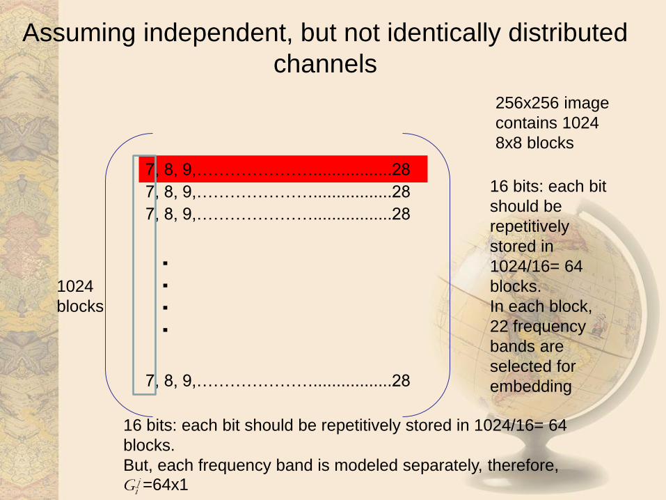
Assuming independent, but not identically distributed

channels

7, 8, 9,………………….................28

7, 8, 9,………………….................28

7, 8, 9,………………….................28

7, 8, 9,………………….................28

.

.

.

.

256x256 image

contains 1024

8x8 blocks

1024

blocks

16 bits: each bit

should be

repetitively

stored in

1024/16= 64

blocks.

In each block,

22 frequency

bands are

selected for

embedding

16 bits: each bit should be repetitively stored in 1024/16= 64

blocks.

But, each frequency band is modeled separately, therefore, Gi

j =64x1

In our proposed scheme, in view of the attack,each frequency band is

modeled separately

where Jmax is the maximum number of selected frequency bands, and rji

is defined as given

where Qji, is defined as the sample vector of all DCT coefficients in

different 8×8 blocks that correspond to a single bit i and the jth

frequency band.

The values of c and σ are estimated from the received watermarked

image at the decoding stage.

Proposed watermark extraction

max1,2,...j

j

i ir j Jr

jQi

c

c c

j

i

Y α s Y α s

σr

k

k kk k k k k k

kk

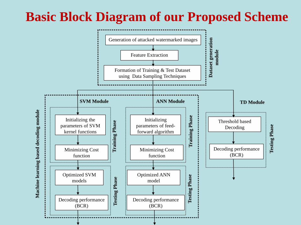
Basic Block Diagram of our Proposed Scheme

Generation of attacked watermarked images

Formation of Training & Test Dataset

using Data Sampling Techniques

Feature Extraction

Initializing the

parameters of SVM

kernel functions

Minimizing Cost

function

SVM Module

Tes

tin

g P

hase

Optimized SVM

models

Decoding performance

(BCR)

Tra

inin

g P

hase

Initializing

parameters of feed-

forward algorithm

ANN Module

Tes

tin

g P

hase

Optimized ANN

model

Decoding performance

(BCR)

Tra

inin

g P

hase

Tes

tin

g P

hase

Threshold based

Decoding

Decoding performance

(BCR)

TD Module

Minimizing Cost

function

Data

set

gen

erati

on

mod

ule

Mach

ine

learn

ing b

ase

d d

ecod

ing m

od

ule

1st Step: Dataset Generation

Type of Images Gray Scale

Number of images 5

Name of Images Baboon, Lena, Trees, Boat & couple

Size of images 256 *256

Size of Message 128 bits

Number of keys 25

Type of Attack Gaussian Attack

Severity of attack σ =10

Dataset of 16000 bits

5 different images

Embed message in each image using 25 different keys

Gaussian noise of σ =10

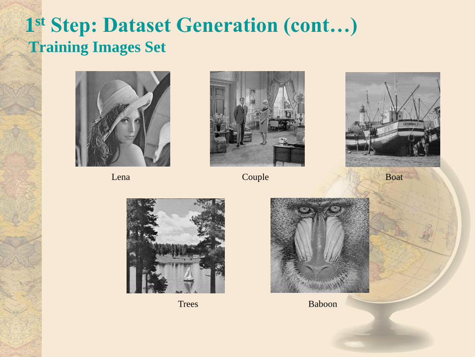
1st Step: Dataset Generation (cont…) Training Images Set

Lena Couple Boat

Trees Baboon

2nd Step: Feature Selection

When Watermarked image is attacked

Message within the image is also corrupted

Feature Extraction

First Method

• Combine all the statistical coefficients ri of each bit in message

and then sum the number of times that bit is repeated in image.

• a numerical value corresponding to each bit.

Second Method

• Keep all 22 ri coefficients as features of the bit

• Add corresponding ri of the same channel for the number of

times each bit is embedded.

• 22 features corresponding to each bit

3rd Step: Data Sampling Techniques

• Self Consistency • Training and Test data is same

• In training phase, the class of watermark bit is known.

• Cross Validation • Training and Test data is different

• 4-fold Jackknife Technique

• Training to test ratio is (3:1)

• Repeat the process 4 times

4th Step: Performance Measure (BCR)

• Performance of Classification Models is evaluated in terms of Bit Correct Ratio (BCR).

• Ratio between number of Bits correctly predicted and that of total number of Bits.

where M represents the original, while M’ represents the decoded message, Lm is the length of the message and represents exclusive-OR operation.

1

',

mL

i ii

m

M MBCR

L

M M

1. SVM based Decoding

2. ANN based Decoding

Intelligent Decoding Schemes

Basics of Support Vector Machine

Input data mapped into a higher dimension by using dot product of

kernel functions.

Decision boundary should be far away from the data of both classes.

Class 1

Class 2

m

1TW x b

1TW x b

0TW x b

2m

W

WClass 2

Class 1 Class 1

Class 2

SVM: An Optimization Problem

For training pairs examples

Decision surface for a linear separable data is :

A vector xi having non zero αi is called a support vector (SV).

Decision boundary is determined only by SVs.

Nonlinear surface:

( , ), , {1, 1},ni i i i

x c x R c

1

( ) . , 0,N

Ti i i i

i

f x c x x ba a

1 1

( ) ( , ) ( ) ( )S S

N N

i i i i i ii i

f x c K x x b c x x ba a

SVM Kernel Functions

Kernel function and mapping into higher dimensional space

Need of Mapping

( , ) .T

i j i jK x x x x , Linear kernel

( , ) [ , ] ,d

i j i jK x x x x r Polynomials kernel

2

( , ) exp( )i j i jK x x x x , RBF kernel

f( )

f( )

f( ) f( ) f( )

f( )

f( ) f( )

f(.) f( )

f( )

f( )

f( ) f( )

f( )

f( )

f( ) f( )

f( )

Input Space Feature Space

1. Details of SVM based Decoding

• Training – SVM classification models are trained for both single as well as 22 features.

– Two data sampling techniques: self-consistency, cross-validation are used.

– We used Different SVM kernel functions Linear, Polynomial and RBF.

• Testing – Trained models are used to test the performance on same or entirely different data.

– Results from SVM models are used to estimate the decoding performance in terms of BCR.

– To minimize the problem of over-fitting in the training of SVM classification models, appropriate size of training and testing data is used .

• Grid Search – The decoding performance of these models is optimized using grid search. Suitable

grid range and step size is estimated for SVM kernels.

– For Poly-SVM, a grid range of C = [2-2 to 22] ,γ = [2-2 to 28] and step size = 0.4

– For RBF-SVM, C = [2-2 to 22], ΔC =0.4, γ = [2-2 to 28], Δγ = 0.4.

– For linear-SVM, C = [2-1 to 25], with ΔC =0.4.

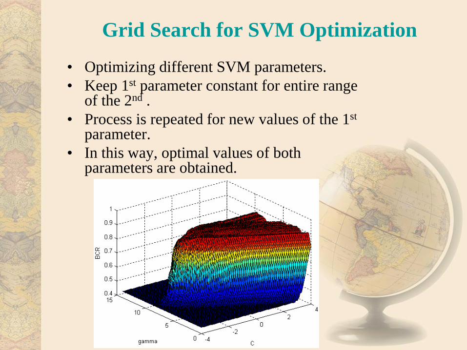
Grid Search for SVM Optimization

• Optimizing different SVM parameters.

• Keep 1st parameter constant for entire range of the 2nd .

• Process is repeated for new values of the 1st parameter.

• In this way, optimal values of both parameters are obtained.

2. Details of ANN Based Decoding

Parameters for ANN Based decoding Method

ANN models are trained for both single as well as 22 features.

Two data sampling techniques: self-consistency, cross-validation are used.

Levenberg-Marquardt Algorithm is used for training

Important parameters : Number of hidden and output layer units, activation functions and

training algorithm.

ANN

Features 1 22

Data Size 16000 16000

Epochs 35 25

Hidden layers 3 [8,4,2] 2 [22,11]

Activation function of Hidden Layer ‘tansig’ ‘tansig’

Activation function of Output Layer ‘pure linear’ ‘pure linear’

Training Algo Levenberg-Marquardt Levenberg-Marquardt

Results and Discussion

1) Implementation Details

2) General Behavior of SVM during Training

3) Self-consistency Performance in terms of BCR

4) Cross-validation Performance in terms of BCR

1). Implementation Details

• Implementation is carried out in MATLAB

• To employ SVM models, MATLAB-based SVM-OSU toolbox is used

• Some of the parameters are optimized using grid search

• To develop ANN classification model, MATLAB built-in ANN toolbox is used.

2). General Behavior of SVM Parameter

Optimization During Training

SVM model Behavior during Grid Search for 22 features

Cyclic Dependency of SVM performance on parameter C

Accuracy does not increase after achieving

a certain level, whatever is the range

• This helps us in focusing on a short range of C, e.g. 0.4 to 0.8

2). General Behavior of SVM during Training

(contd…)

SVM models being trained on 22 features for Self-Consistency

• Gamma dependency

when C is fixed

• Poly & RBF SVMs

forming non linear

hyper plane shows

improved results

• Poly-SVM optimizes

earlier than RBF-SVM

0 8 16 32 64 128 2560.982

0.9835

0.985

0.9865

0.988

0.9895

0.991

0.9925

0.994

0.9955

0.997

0.9985

1

G =0.25 to 256, C is fixed to 1

BC

Rs d

uring T

rain

ing

Behaviour Of SVM models during Training

Linear SVM

Poly SVM

Rbf SVM

3). Self-Consistency Performance (BCR )

Data

Size

(bits)

Hernandez

Scheme

Proposed SVM based Scheme ANN

Linear Poly RBF

Number of Features Number of Features Number of Features Number of Features

1 22 1 22 1 22 1 22

C=1 C=48 γ=1 γ =1 γ =1 γ =256 Epochs=25 Epochs=25

16000

0.9840

0.9843

0.98544

0.9843

1

0.9843

1

0.9842

0.9976

Linear models

classify

linearly, and

therefore, can

not classify

properly in a

high

dimensional

feature space

3). Self-Consistency Performance using

single feature (on different images) Image Type

25 copies each

Data Size (bits)

128 x 25

Hernandez

Scheme

Proposed Scheme

ANN Linear

C = 25.6 Poly

γ = 24 RBF

γ = 1

Lena 3200 0.9931 0.9934 0.9934 0.9934 0.9934

Boat 3200 0.9819 0.9819 0.9819 0.9819 0.9822

Couple 3200 0.9856 0.9856 0.9856 0.9856 0.9853

Trees 3200 0.9822 0.9828 0.9828 0.9828 0.9828

Baboon 3200 0.9772 0.9778 0.9778 0.9778 0.9772

Gaussian noise

attack distorts the

modeling of DCT

coefficients

severely in

textured image as

compared to

relatively smooth

images

3). Self-Consistency Performance using

22 features (on different images)

Image Type

25 copies each

Data Size (bits)

128 x25

Hernandez Scheme Proposed Scheme SVM Models ANN

Linear

C = 25.6

Poly

γ=27

RBF

γ=28

Lena 3200 0.9931 0.9962 1 1 0.9997

Boat 3200 0.9819 0.9825 1 1 0.9975

Couple 3200 0.9856 0.9862 1 1 0.9975

Trees 3200 0.9822 0.9841 1 1 0.9975

Baboon 3200 0.9772 0.9784 1 1 0.9959

Nonlinear

models classify

nonlinearly, and

therefore, can

classify

properly in a

high

dimensional

feature space

4). Cross-Validation results:

( single feature on train/test data)

Type of

SVM

C Gamma

γ

Training Data

(bits)

BCR Avg. BCR Test Data

(bits)

BCR Average

BCR

Linear

0.5 to 1024 - 4000 0.9832

0.9843

12000 0.9847

0.9843 0.5 to 1024 - 4000 0.9812 12000 0.9853

0.5 to 1024 - 4000 0.9878 12000 0.9832

0.5 to 1024 - 4000 0.9850 12000 0.9841

Poly

0.76 to 1.7 1 to 16 4000 0.9832

0.9843

12000 0.98467

0.9843 0.76 to 1.7 1 to 16 4000 0.9812 12000 0.98533

0.76 to 1.7 1 to 16 4000 0.9878 12000 0.98317

0.76 to 1.7 1 to 16 4000 0.9850 12000 0.98408

RBF 1 to 1.74 1.74 to 16 4000 0.9832

0.9843

12000 0.98467

0.9843 1 to 1.74 1.74 to 16 4000 0.9812 12000 0.98533

1 to 1.74 1.74 to 16 4000 0.9878 12000 0.98317

1 to 1.74 1.74 to 16 4000 0.9850 12000 0.98408

ANN

- - 4000 0.983

0.9843

12000 0.98433

0.9838 - - 4000 0.98175 12000 0.984

- - 4000 0.9875 12000 0.983

- - 4000 0.98475 12000 0.98392

4). Cross-Validation results: 22 feature (train/test data)

Type of

SVM

C Gamma

γ

Training Data

(bits)

BCR Average

BCR

Test Data

(bits)

BCR Average

BCR

Linear

48.503 - 4000 0.9852

0.9853

12000 0.9855

0.9855 48.503 - 4000 0.9832 12000 0.98617

111.43 - 4000 0.9868 12000 0.9850

111.43 - 4000 0.9860 12000 0.98525

Poly

0.4 to 2 194 4000 1

1

12000 1

1 0.4 to 2 194 4000 0.9998 12000 1

0.4 to 2 194 4000 1 12000 1

0.4 to 2 194 4000 1 12000 1

RBF

0.75786 5.2768 4000 0.9850

0.9877

12000 0.98483

0.9840 1.3195 6.9644 4000 0.9875 12000 0.98475

1 1.7411 4000 0.9868 12000 0.98333

2.2974 9.1896 4000 0.9915 12000 0.98325

ANN

- - 4000 0.9992

0.9997

12000 0.9762

0.9746

- - 4000 0.9998 12000 0.9727

- - 4000 0.9998 12000 0.9768

- - 4000 0.9998 12000 0.9727

Hernandez

- - 4000 0.983

0.9840

12000 0.98433

0.9840 - - 4000 0.9805 12000 0.98517

- - 4000 0.98775 12000 0.98275

- - 4000 0.98475 12000 0.98375

4). Cross Validation Performance Comparison

(Single & 22 Features)

0.97

0.975

0.98

0.985

0.99

0.995

1

BCR Train data BCR Test Data

Hernandez

Linear SVM

PolySVM

Rbf SVM

ANN

0.982

0.9825

0.983

0.9835

0.984

0.9845

BCR Train Data BCR Test Data

Hernandez

Linear SVM

PolySVM

Rbf SVM

ANN

Cross-validation Performance using single feature

Cross-validation Performance using 22 feature

Shows the

Generalization

of PolySVM

Conclusion • We practically demonstrate that the use of ML techniques

like SVM attains high performance than traditional decoders in presence of an attack.

• Exploitation of individual frequency bands shows performance improvement

• General order of Performance in terms of BCR is:

SVM > ANN >Threshold Decoding

and for different Kernels of SVM:

PolySVM ≈ RbfSVM > LinearSVM

• When an application of watermarking is changed, and consequently, new attacks are anticipated,

• The re-training of the ML based decoding makes it adaptive by learning the distortion incurred on the features.