Ies

Ja

b

W

a

ARRAA

KFDPARR

I

piebhtsc

didrms

(t

h1

Applied Soft Computing 24 (2014) 50–62

Contents lists available at ScienceDirect

Applied Soft Computing

j ourna l ho me page: www.elsev ier .com/ locate /asoc

ntelligent feedback linearization control of nonlinearlectrohydraulic suspension systems using particlewarm optimization

imoh O. Pedroa,∗, Muhammed Dangora, Olurotimi A. Dahunsia, M. Montaz Alib

School of Mechanical, Industrial and Aeronautical Engineering, University of the Witwatersrand, Johannesburg, South AfricaSchool of Computational and Applied Mathematics, Faculty of Science, and TCSE, Faculty of Engineering and Built Environment, University of theitwatersrand, Johannesburg, South Africa

r t i c l e i n f o

rticle history:eceived 23 February 2013eceived in revised form 14 May 2014ccepted 16 May 2014vailable online 27 June 2014

a b s t r a c t

The core factors governing the performance of active vehicle suspension systems (AVSS) are the inherenttrade-offs involving suspension travel, ride comfort, road holding and power consumption. In addition tothis, robustness to parameter variations is an essential issue that affects the effectiveness of highly non-linear electrohydraulic AVSS. Therefore, this paper proposes a nonlinear control approach using dynamicneural network (DNN)-based input–output feedback linearization (FBL) for a quarter-car AVSS. The gainsof the proposed controllers and the weights of the DNNs are selected using particle swarm optimization

eywords:eedback linearizationynamic neural networksarticle swarm optimizationctive vehicle suspension systemside comfort

(PSO) algorithm while addressing simultaneously the AVSS trade-offs. Robustness and effectiveness ofthe proposed controller were demonstrated through simulations.

© 2014 Elsevier B.V. All rights reserved.

oad holding

ntroduction

Vehicle suspensions are subsystems that aim to improve theerformance of an automobile by isolating the vehicle from road-

nduced disturbances, improving passenger ride comfort, andnhancing the road holding performance of the vehicle. However,etter ride comfort demands a softer suspension and superior roadolding requires a stiffer suspension. The desire to manage theserade-offs has led to the development of active vehicle suspensionystems (AVSS) which incorporates an actuator to deal with theseompromises in real time [1].

AVSS are highly nonlinear systems with complex actuatorynamics and need to be designed carefully to manage its sensitiv-

ty to parameter variations. Nonlinear AVSS have been successfullyesigned with linear controllers [1]. However, these controllers lack

obustness when dealing with variations in vehicle speed, sprungass and tyre load. On the contrary, nonlinear control schemes

uch as Fuzzy Logic Control (FLC), backstepping, FBL and neural

∗ Corresponding author. Tel.: +27 117177317; fax: +27 117177049.E-mail addresses: jimoh.pedro@wits.ac.za, jimoh.olarewaju.pedro@gmail.com

J.O. Pedro), Muhammed.Dangor@students.wits.ac.za (M. Dangor),undedahunsi@gmail.com (O.A. Dahunsi), montaz.ali@wits.ac.za (M.M. Ali).

ttp://dx.doi.org/10.1016/j.asoc.2014.05.013568-4946/© 2014 Elsevier B.V. All rights reserved.

network (NN)-based control have been able to deal with theseissues more effectively [2–10]. In contrast to linear controllers,nonlinear control methods generate an input that aims to removeor significantly reduce the effects of nonlinearities in the system.

The nonlinear AVSS model presented by Shi et al. [3] incor-porated a servo-hydraulic system controlled by a combination ofsliding mode and feedback linearization control methods. Thiseffort and those of Yagiz and Sakman [2] and Chamseddine et al.[9] using sliding mode control were plagued with chattering chal-lenges.

Backstepping control has been performed by [4,5,10] for half-carand full-car models respectively. Their solutions showed a signif-icant improvement over the passive vehicle suspension system(PVSS) and additionally provided an adequate bandwidth wherethey were able to reject a large range of road disturbances, whichemphasizes the robustness of this control technique.

However, these preceding control laws are fundamentally basedon the mathematical models which have been chosen to beeither linear or nonlinear. In the case of backstepping, highlynonlinear and realistic models would require rigorous interlaced

backstepping which may in some cases prove impossible to solve.Furthermore, the associating zero-dynamics present in real modelsmay be unstable under certain conditions. Furthermore, the sys-tems may not be completely understood in reality and this would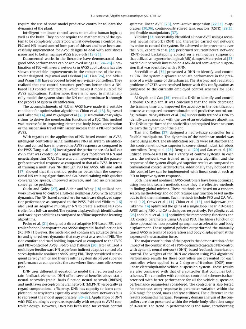

oft Com

rd

wtFci

gbstarbAct

carwoA

ittAggo[tcc

wdrataa

t(iramsqpu

tnarptwt

J.O. Pedro et al. / Applied S

equire the use of some model predictive controller to learn theynamics of the plant.

Intelligent nonlinear control seeks to emulate human logic asell as the brain. They do not require the mathematics of the sys-

em to be completely understood whilst developing a control law.LC and NN-based control form part of this set and have been suc-essfully implemented for AVSS designs to deal with robustnessssues and to better manage AVSS trade-offs [13–25].

Documented works in the literature have demonstrated thatood AVSS performances can be achieved using FLC [24–26]. Com-ination of FLC with neural networks in AVSS applications has alsohown remarkable improvements in the robustness of the con-roller designed. Rajeswari and Lakshmi [14], Lian [26], and Aldairnd Wang [18] have proposed hybrid neuro-fuzzy controllers. Theyealized that the control structure performs better than a NN-ased PID control architecture, which makes it more suitable forVSS applications. Furthermore, there is no need to mathemati-ally model the system since the NN can approximate it throughhe process of system identification.

The accomplishments of FLC in AVSS have made it a suitableandidate for optimization algorithms. Chiou et al. [13], Rajeswarind Lakshmi [14], and Pekgökgöz et al. [25] used evolutionary algo-ithms to derive the membership functions of a FLC. This methodas successful in improving either the body-heave acceleration

r the suspension travel with larger success than a PID-controlledVSS.

With regards to the application of NN-based control to AVSS,ntelligent controllers using multilayer NNs in system identifica-ion and control have improved the AVSS response as compared tohe PVSS. Tang et al. [15] investigated the performance of a half-carVSS that was controlled using a multilayer feedforward NN andenetic algorithm (GA). There was an improvement in the passen-er’s seat vertical response as compared to that of a PVSS. In termsf training a multilayer NN through PSO for AVSS, Alfi and Fateh17] showed that this method performs better than the conven-ional NN training algorithms and GA-based training with quickeronvergence speeds, improved accuracy, and had no prematureonvergence problem.

Guclu and Gulez [27], and Aldair and Wang [18] utilized net-ork inversion to control a full-car nonlinear AVSS with actuatorynamics. The NN-based controllers for each case displayed supe-ior performance as compared to the PVSS. Eski and Yildirim [16]lso used an adaptive multilayer NN to create a robust PID con-roller for a full-car model. The system displayed high identificationnd tracking capabilities as compared to offline supervised learninglgorithms.

Pedro et al. [21] designed a direct adaptive NN-based FBL con-roller for nonlinear quarter-car AVSS using radial basis function NNRBFNN). However, the model did not contain any actuator dynam-cs and ignored zero dynamics that may exist as a result of FBL. Theide comfort and road holding improved as compared to the PVSSnd PID-controlled AVSS. Pedro and Dahunsi [20] later utilized aultilayer feedforward NN to perform indirect adaptive control of a

ervo-hydraulic nonlinear AVSS using FBL. They considered subse-uent zero dynamics and their resulting system displayed superiorerformance as compared to the case where linear controllers weresed.

DNN uses differential equation to model the neuron and con-ain feedback elements. DNN offers several benefits above staticeural networks (radial basis function neural network (RBFNN)nd multilayer perceptron neural network (MLPNN)) especially asegard computational efficiency. DNN has capacity to learn com-

lex nonlinear systems especially when static neural networks failso represent the model appropriately [30–32]. Application of DNNith PSO training is very rare, especially with respect to AVSS con-

roller design. However, DNN has been used for various control

puting 24 (2014) 50–62 51

systems: linear AVSS [23], semi-active suspension [22,33], evap-orators [30,36], continuously stirred tank reactors (CSTR) [29,35]and flexible manipulators [37].

Yildirim [23] successfully identified a linear AVSS using a recur-rent neural network (RNN) and thereafter carried out networkinversion to control the system. He achieved an improvement overthe PVSS. Zapateiro et al. [22] performed recurrent neural network(RNN)-based backstepping control on a semi-active suspensionthat utilized a magnetorheological (MR) damper. Metered et al. [33]carried out network inversion on a MR-based semi-active suspen-sion that was identified with a RNN.

Becerikli et al. [34] presented a DNN to identify and controla CSTR. The system displayed adequate performance in the pres-ence of a wide range of disturbances. The start-up and regulationproblems of CSTR were resolved better with this configuration ascompared to the currently employed control schemes for CSTRtanks.

Al Seyab and Cao [35] created a DNN to identify and controla double CSTR plant. It was concluded that the DNN decreasedthe training time and improved the accuracy in the identificationprocess as compared to conventional model predictive control con-figurations. Nanayakkarra et al. [36] successfully trained a DNN toidentify an evaporator with the use of an evolutionary algorithm.The DNN outperformed the static NNs and required fewer neuronsto learn the dynamics of the plant.

Tian and Collins [37] designed a neuro-fuzzy controller for aflexible manipulator. The dynamics of the nonlinear model waslearnt using a DNN. The identification results were satisfactory andthis control method was superior to conventional industrial robotscontrollers. Deng et al. [28], Deng et al. [29] and Garces et al. [30]utilized DNN-based FBL for a variety of control systems. In eachcase, the network was trained using genetic algorithm and theresponse of the system displayed superior results as compared toconventional control architectures. Additionally they noticed thatthis control law can be implemented with linear control such asPID to improve system response.

Both linear and nonlinear AVSS controllers have been optimizedusing heuristic search methods since they are effective methodsin finding global minima. These methods are based on a randomsearch methodology and do not require any function based meth-ods to find the minimum. Such methods include PSO and GA. Waiet al. [12], Crews et al. [11], Chiou et al. [13], and Rajeswari andLakshmi [14] optimized the gains of a single loop linear PID-basedAVSS using PSO and GA techniques respectively. Pekgökgöz et al.[25] and Chiou et al. [13] optimized the membership functions andFLC control parameters using GA and PSO. The fitness function ofthese approaches incorporated sprung mass acceleration and bodydisplacement. These optimal policies outperformed the manuallytuned AVSS in terms of acceleration and body displacement at theexpense of the actuation force.

The major contribution of the paper is the demonstration of theimpact of the combination of a PSO-optimized cascaded PID controlwith dynamic neural network (DNN)-based feedback linearizationcontrol. The weights of the DNN are chosen using PSO algorithm.Performance results for these controllers are presented for eachcontroller when applied to a 2 degree-of-freedom (DOF) non-linear electrohydraulic vehicle suspension system. These resultsare also compared with that of a controller that combines bothschemes. The controller with combined controlled schemes is char-acterized with better performance for all the vehicle suspensionperformance parameters considered. The controller is also testedfor robustness using response to parameter variation within the

20% range for speed, mass and tyre stiffness. The difference in theresults obtained is marginal. Frequency domain analysis of the con-trollers are also presented within the whole-body-vibration rangeof 0–80 Hz. The trend in performance is the same, corroborating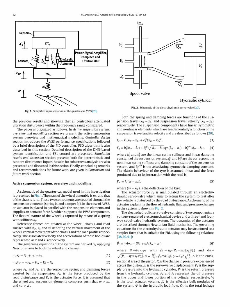

52 J.O. Pedro et al. / Applied Soft Computing 24 (2014) 50–62

tv

ossbdsrrpaf

A

iosasTw

swtr

N

m

m

werta

Fig. 1. Simplified representation of the quarter-car AVSS [20].

he previous results and showing that all controllers attenuatedibration disturbance within the frequency range considered.

The paper is organized as follows. In Active suspension system:verview and modelling section we present the active suspensionystem overview and mathematical modelling. Controller designection introduces the AVSS performance specifications followedy a brief description of the PID controller. PSO algorithm is alsoescribed in this section. Detailed description of the DNN-basedystem identification and FBL control are presented. Simulationesults and discussion section presents both for deterministic andandom disturbance inputs. Results for robustness analysis are alsoresented and discussed in this section. Finally, concluding remarksnd recommendations for future work are given in Conclusion anduture work section.

ctive suspension system: overview and modelling

A schematic of the quarter-car model used in this investigations presented in Fig. 1. The mass of the wheel assembly is mu and thatf the chassis is ms. These two components are coupled through theuspension elements (spring ks and damper bs). In the case of AVSS,n actuator is placed in parallel with the suspension elements andupplies an actuator force Fa which supports the PVSS components.he flexural nature of the wheel is captured by means of a springith stiffness kt.

Reference frames are created at the wheel, chassis and roadurface with xw , xc and w denoting the vertical movement of theheel, vertical movement of the chassis and the road profile respec-

ively. The associated velocity and accelerations of these bodies areepresented as x and x, respectively.

The governing equations of the system are derived by applyingewton’s laws to both the wheel and chassis:

sxc = Fks + Fbs − Fa, (1)

uxw = −Fks − Fbs + Fa + Fw, (2)

here Fks and Fbs are the respective spring and damping forces

xerted by the suspension, Fw is the force produced by theoad disturbance and Fa is the actuator force. It is assumed thathe wheel and suspension elements compress such that w > xwnd xw > xc .

Fig. 2. Schematic of the electrohydraulic servo-valve [20].

Both the spring and damping forces are functions of the sus-pension travel (xw − xc) and suspension travel velocity (xw − xc),respectively. The suspension components have linear, symmetricand nonlinear elements which are fundamentally a function of thesuspension travel and its velocity and are described as follows [20]:

Fs = kls(xw − xc) + knls (xw − xc)3, (3)

Fb = bls(xw − xc) + bnls√

|xw − xc |sgn(xw − xc) − bsyms |xw − xc |, (4)

where kls and bls are the linear spring stiffness and linear dampingconstant of the suspension system, knls and bnls are the correspondingnonlinear spring stiffness and damping constant of the suspensionsystem, and bsyms is the associating symmetric damping constant.The elastic behaviour of the tyre is assumed linear and the forceproduced due to its interaction with the road is:

Fw = kt(w − xw), (5)

where (w − xw) is the deflection of the tyre.The actuator force Fa is manipulated through an electrohy-

draulic servo-valve which aims to return the system to rest afterthe vehicle is disturbed by the road disturbance. A schematic of theactuator explaining the flow of hydraulic fluid and pressure changesin the system is shown in Fig. 2.

The electrohydraulic servo-valve consists of two components: avoltage-regulated electromechanical device and a three-land four-way spool-valve hydraulic system. The dynamics of the actuatorare described through Newtonian fluid mechanics. The governingequations for the electrohydraulic actuator may be structured to asimpler form that is suitable for FBL using the following relations[38,39,41]:

PL = �˚xv − ˇPL + ˛A(xw − xc), (6)

where = �1 × �2 with �1 = sgn(Ps − sgn(xv)PL) and �2 =√(Ps − sgn(xv)PL), = 4ˇe

Vt, ˇe = ˛Ctp, � = CdS

√1� . A is the cross-

sectional area of the piston, PL is the change in pressure experiencedacross the piston, xv is the servo-valve displacement, Ps is the sup-ply pressure into the hydraulic cylinder, Pr is the return pressure

from the hydraulic cylinder, Pu and Pl represent the oil pressurein the upper and lower portion of the cylinder respectively, Vt

is the total actuator volume, ˇe is the effective bulk modulus ofthe system, is the hydraulic load flow, Ctp is the total leakage

J.O. Pedro et al. / Applied Soft Com

Table 1System parameters for the quarter-car model [20,40,41].

Parameter Numerical value

Chassis or sprung mass, ms 290 kgWheel or unsprung mass, mu 40 kgSuspension spring linear stiffness, kls 2.35 × 104 N/mSuspension spring nonlinear stiffness, knls 2.35 × 106 N/m3

Tyre stiffness, kt 190 × 105 N/mSuspension linear damping coefficient, bls 700 Ns/mSuspension nonlinear damping coefficient, bnls 400 Ns0.5/m0.5

Suspension symmetric damping coefficient, bsyms 400 Ns/mActuator parameters, (˛, ˇ, �) 4.515 × 1013, 1, 1.545 × 109

Piston area, A 3.35 × 10−4 m2

cs

cfi

x

wo

ebtp

w

ww

− x3)

x4 −

Supply pressure, Ps 10,342,500 PaTime constant, � 1/30 sServo valve gains, kv 0.001 m/V

oefficient of the piston, Cd is the discharge coefficient, S is thepool-valve area gradient and � is the hydraulic fluid density.

In order to reduce complexity, it is assumed that the electrome-hanical device that controls the motion of the spool valve is arst-order element with a time constant � and is described as:

˙ v = 1�

(Kvu − xv), (7)

here Kv is the valve gain and u is the control input voltage. Valuesf the parameters used in the quarter-car model are given in Table 1.

The performance of the AVSS is investigated as the vehicle trav-ls over a deterministic road bump at a speed of 40 km/h. The roadump has a sinusoidal profile with a length of 2.5 m and ampli-ude of 11 cm. The equation describing the profile of the bump isresented in Eq. (8) and is displayed in Fig. 3

(t) =

⎧⎨ a(1 − cos 2�(V/�)t)

20.45 ≤ t ≤ 0.9,

(8)

f3(x) = 1ms

[kls(x2 − x1) + knls (x2 − x1)3 + bls(x4

f4 (x) = 1mu

[−kls(x2 − x1) − knls (x2 − x1)3 − bls(

⎩0 otherwise,

here a is the bump height, V is the vehicle speed, � is the halfavelength of the sinusoidal road undulation [20].

Fig. 3. Road disturbance profile.

puting 24 (2014) 50–62 53

The system may be further rearranged into a state-space formby defining the following state variables: x1 = x3, x1 = x3, xw = x4,xw = x4, x5 = PL, and x6 = xv [20]:

x = f(x) + g(x)u + w(x), (9)

y = h(x) = x1 − x2, (10)

where the state vector is given by x = [ x1 x2 x3 x4 x5 x6 ]T .The system matrices f and g are denoted by:

f(x) = [ f1 f2 f3 f4 f5 f6 ]T , (11)

g(x) =[

0 0 0 0 0kv

�

]T. (12)

The disturbance matrix w is represented by:

w(x) =[

0 0 0w(t)mu

kt 0 0]T. (13)

The elements of these matrices are as follows [20]:

f1(x) = x3, (14)

f2(x) = x4, (15)

− bsyms |x4 − x3| + bnls√

|x4 − x3|sgn(x4 − x3) − Ax5

], (16)

x3) + bsyms |x4 − x3| − bnls√

|x4 − x3|sgn(x4 − x3) + Ax5

], (17)

f5(x) = �˚x6 − ˇx5 + A(x3 − x4), (18)

f6(x) = 1�

(−x6). (19)

Controller design

AVSS performance specifications

The fundamental objective of the controller is to return the sys-tem to steady state after being disturbed by a deterministic roadbump (Eq. (8)). The controller must also satisfy the following per-formance specifications for the AVSS [20]:

1. The controller should demonstrate good low frequency disturb-ance rejection.

2. Satisfactory transient response with minimal oscillations afterthe disturbance has disappeared; that is:• the rise time should not be greater than 0.1 s.• the maximum overshoot should be less than 5%.• and zero steady-state error.

3. The body-heave acceleration, x1, should be less than 4.5 m/s2 inorder to keep the system in the Less Discomfort region as [43].

4. The suspension travel, y = (x1 − x2), must remain within ±0.1 m.

5. The control voltage is limited to ±10 volts.6. The maximum actuation force, Famax , must be less than the static

weight of the vehicle.7. For good road holding, the dynamic load that is transmitted from

the road should be less than the static weight of the vehicle, i.e.,Ftyre < msg.

8. The controller should minimize a performance index whichincludes suspension travel (disturbance rejection), body-heaveacceleration (ride comfort), wheel deflection (road holding),actuation force and control input voltage (powerconsumption);

54 J.O. Pedro et al. / Applied Soft Co

P

ttec

eibsht

e

F

e

u

wlor

P

Dcpe

Fig. 4. Architecture of the multi-loop PID-controlled quarter-car AVSS.

which is given by:

J = 1T

∫ T

0

[(x1

x1max

)2

+(

(x2 − w)(x2 − w)max

)2

+(

y

ymax

)2

+(FaFamax

)2+

(u

umax

)2]dt, (20)

where J is the overall performance index; the first term is relatedto the vehicle ride comfort; the second term is related to theroad holding properties; the third term is related to the sus-pension travel (rattle space); the fourth and fifth terms arerelated to power consumption respectively. x1max , (x2 − w)max,ymax, Famax , umax are maximum allowable body-heave accelera-tion, road holding parameter, suspension travel, actuation forceand control input voltage respectively. T is the final simulationtime.

ID controller design

The PID control for the AVSS comprises of two control loops:he outer loop, which regulates the controlled variable (suspensionravel, y) and the inner loop which ensures stable operations of thelectrohydraulic actuator [1]. A schematic of the multi-loop PIDontrol system is shown in Fig. 4.

The setpoint yd is set to zero to address a regulation problem,1 and e2 are error signals that will be minimized in the outer andnner control loops respectively, Fa is the actuator force that wille regulated in the inner control loop with Fd being its respectiveetpoint, and u is the control input voltage that is passed into theydraulic actuator of the AVSS. PID controllers operate accordingo the following equations:

1(t) = yd(t) − y(t) = yd(t) − xw(t) + xc(t), (21)

d(t) = KPe1(t) + KDde1(t)dt

+ KI

∫ T

0

e1(t)dt, (22)

2(t) = Fd(t) − Fa(t), (23)

(t) = kpe2(t) + kdde2(t)dt

+ ki

∫ T

0

e2(t)dt, (24)

here KP and kp are the proportional gains of the outer and inneroops respectively; KI and ki are the corresponding integral gainsf the controllers; and KD and kd are the derivative gains of theespective control loops.

roposed control approach

The proposed controller architecture is presented in Fig. 5. The

NN predicts the response of the plant for a specified input. Theontroller performs FBL on the trained DNN with the intention ofroducing a control signal that cancels out the system’s nonlin-arities. The FBL controller is augmented with a multi-loop PID

mputing 24 (2014) 50–62

controller to achieve improved performance [30]. PSO algorithmis thereafter used to optimize the PID gains, FBL control parame-ters and the DNN weightings in order to obtain an optimal controllaw that best manages the trade-offs associated with the AVSS. Rdis the desired suspension travel as shown in Fig. 5. The rest of thissubsection is devoted to providing a detailed presentation of thesystem identification and controller design.

DNN-based nonlinear system identificationFig. 6 shows the structure of a typical DNN. The dynamics of the

neurons are described by a first-order differential equation witha time constant �. Additionally, each neuron receives feedbackfrom neurons in its respective hidden layer xt−1 of the neural net-work, as well as from the input layer of the neural network ut. Boththe network and neuron-to-neuron inputs are essentially added tothe right hand side of the differential equation that describes thedynamics of the neuron.

The output of each neuron is passed through an activation func-tion �(x) before it is fed back to each neuron in the correspondinghidden layer. Additionally, each neuron has two external inputs:control input u and a delayed system state xt−1, each of which pos-sesses its own associating weighting value. Hence, a neuron in thefirst hidden layer of the neural network is described by:

x = −�x + W�(x) + �ut + �xt−1, (25)

where x is a vector denoting the outputs of each neuron, � is adiagonal matrix containing the time constants for each neuron inthe hidden layer, �(x) is the vector containing the neuron outputsafter it had passed through the activation function, W is the inter-connecting neuron weights, ut is a vector that holds the variouscontrol input signals that are being passed into the real system,� is a matrix which holds the weighting contributions that eachcontrol input has on each neuron, xt−1 is a vector that holds theactual system output or delayed output at the previous time step,and � is the contribution of these aforementioned outputs on eachneuron.

The output layer of the DNN comprises of a single neuron andis fundamentally an algebraic equation, which is essentially theweighted sum of the neuron outputs from the preceding hiddenlayer x. Thus, the neuron in this layer is described as follows:

y = hn(x) =nn∑i=1

wixi, (26)

where xi is a vector comprising of the output of the ith neuron fromthe hidden layer, wi is the associating weighting contribution of theith neuron in the hidden layer, nn is the number of neurons in thehidden layer.

In order to further simplify the model and the subsequent com-putation, the output of the network y will depend solely on theoutput from the first neuron in the preceding hidden layer. Conse-quently, the output layer will be simplified to:

y = h1 = w1x1. (27)

Furthermore, the selection of the network parameters such as:the number of hidden layers, size of the hidden layer nn and theactivation function �(·) is based on two items: the network sta-bility and the method of pruning [32]. In the course of pruning,the primary network parameters such as the hidden layer size areincreased until the predicted system output y stops changing topol-ogy with further increase in the hidden layer size. Garces et al.

[30] suggest that �(·) should be bounded to within ±1 so thatthe free response of the DNN converges to zero and thus stabi-lizes once the networks inputs are removed. Hence, the hyperbolictangent function is chosen as activation function �(·) to meet this

J.O. Pedro et al. / Applied Soft Computing 24 (2014) 50–62 55

Fig. 5. Architecture of the DNN-based FBL control augmented with PSO algorithm.

ibing t

ct

oepisi

ttahitiVattfcp

tification. The structure of the DNN is summarized in Table 2.This DNN is trained offline using PSO algorithm. PSO was first

introduced by Kennedy and Eberhart [44] and they mimic the foodsearching process of swarms. As in the swarm of animals, each

Table 2Configuration of applied dynamic neural networks for the quarter-car system.

Property Numerical value

Fig. 6. Schematic descr

ondition. The next condition may only be fulfilled after the selec-ion of appropriate input–output data.

An important step in system identification is to select a rangef input–output data that covers the range of signals that will bencountered in reality. In indirect adaptive control the DNN mustredict the output of the suspension system for a given set of control

nput voltage. White-Band-Limited (WBL) noise is used to create aet of input data because it can successfully create a random set ofnput signals which span the space of the expected input signals.

Selection of an appropriate data set is a rather rigorous processhat requires several conditions to be met. Firstly, the dynamics ofhe subsystem with the smallest time constant must be capturednd this demands that the seed strength of the WBL be significantlyigh. Secondly, the input data must span the space of all possible

nput voltages, which is known to be in the range of ±10 V. Similarly,he set of suspension travel output must span the region in which its expected to operate, which corresponds to ±0.1 m. “Whole Bodyibration” (WBV) frequency range is classified to be between 0.5nd 80 Hz. Human occupants are susceptible to vibrations withinhis range. The resonant frequency range for the suspension sys-em is smaller and fits into both the WBV as well as, the “lowrequency” range. It is thus paramount that the system identifi-ation input covers these frequencies [42]. In order to satisfy the

receding conditions, WBL was set as follows:

i. Control input u operates within ±10 V.ii. WBL has the following properties:

he operation of a DNN.

• Seed strength of 22,641.• 0.001 s sampling time.

iii. Hyperbolic Tangent is used for the activation function �(x) asthis ensures the DNN stability [28–30].

With regards to pruning and the choice of hidden layer size nn theresponse of the DNN is analyzed for a range of nn starting fromone. The network size was increased until satisfactory results wereattained for a credible range of randomly selected network param-eters. Fig. 7 shows the general trend of the suspension travel outputfor the various hidden layer sizes. It is evident from this figurethat a hidden layer size nn of 8 is capable of capturing the sensi-tive dynamics of the system as it can pick up the sudden rate ofchange of suspension travel more adequately than the 4-neuronand 6-neuron configurations. Hence, it is suitable for system iden-

Number of hidden layers 2Number of neurons in first hidden layer 8Number of delayed system inputs 1Number of delayed system outputs 1

56 J.O. Pedro et al. / Applied Soft Computing 24 (2014) 50–62

0 5 10 15 20

-0.06

-0.04

-0.02

0

0.02

0.04

0.06

0.08

Time (s)

Susp

ensi

on T

rave

l (m

)

Actual 4 neurons6 neurons8 neurons

apdpAtoporci

S

S

SS

S

S

0 20 40 60 80 100 120 140 16010

-6

10-5

10-4

10-3

Numbe r o f Iterations

Mea

n Sq

aure

d E

rror

Before controller design can begin, the stability of the DNNmodel must be ensured. Deng et al. [28], Deng et al. [29] and Garceset al. [30] suggest that the DNN stability will be guaranteed if thefollowingconditions hold:

Table 3Parameters used during the PSO implementation to obtain the DNN model.

Parameters Value

Population size 200Maximum number of iterations 200Velocity inertia weight (w1) 0.5

Fig. 7. Quarter-car suspension travel output for different hidden layer sizes.

nimal or particle searches a search space for a specific item. Eacharticle thereafter relays their success in relation to finding theesired item. Each particle will subsequently travel towards theosition of the particle with the highest success at various speeds.t the same time, it will examine the area for a personal best posi-

ion to achieve. The position of the particle refers to the locationf the particle in n dimensional space where n is the number ofarameters that are being altered. Searching towards the vicinityf the best particle and in the neighbourhood its personal best areeferred to as the global and local searches respectively. The pro-ess repeats itself until the stopping criterion is met. The algorithms summarized in the following steps [17]:

tep 1: Produce a random population of particles using the uniformdistribution.

tep 2: Provide an initial small velocity to each particle usingpseudo-random normal distributions.

tep 3: Choose the fittest particle as the best particle.tep 4: If the stopping criteria has been met, then stop the algo-

rithm, otherwise proceed to Step 5.tep 5: Adjust the local and global search parameters according to:

wlocal = w1

(n

nmax

), (28)

wglobal = w2

(1 − n

nmax

), (29)

where wlocal , and wglobal are the local and global searchparameters respectively; whilst w1 and w2 are the maxi-mum local and global search weighting respectively. n andnmax are the current iteration and maximum number ofiterations respectively.

tep 6: Compute the new positions of each particle in the searchspace using:

X(t + 1) = X(t) + V(t + 1), (30)

where X is a matrix comprising of the neural networkparameters, V is a matrix consisting of velocity as eachparameter varies

V(t + 1) = w1V(t) + wlocal × rand1(Pbest − X(t)) + wglobal

× rand2(Gbest − X(t)), (31)

where Gbest denotes the vector containing the parame-ters of the global best particle, Pbest represents the matrix

Fig. 8. Evolution of the fitness function, (MSE), during the offline PSO-optimizedtraining of the DNN.

containing the personal best parameters of each particle.rand1 and rand2 are pseudo-random numbers.

Step 7: If the fitness of its new position is better than the fitness ofits personal best, replace its personal best position with itscurrent position and proceed to Step 8, otherwise continuestraight to Step 8 without any adjustments.

Step 8: Find the fittest particle in the population and choose it asthe best particle and return to Step 4.

In this learning process, the DNN parameters �, W, �, and � are theproblem variables that are determined by the PSO algorithm. � is a1 × 8 vector with ˇn denoting the time constant of the nth neuronfrom the 8 present in the first hidden layer. The same applies to �and � as well. W is the weighting matrix that connects each of theneurons of the hidden layer to each other and it is a square 8 × 8matrix with Wjh denoting the feedback weighting of the hth neuroninto the jth neuron.

The objective function of the PSO algorithm during the systemidentification process is the mean square error (MSE) of the devia-tion between the actual and predicted outputs [20]:

J = MSE = 12N

N∑i=1

(yi − yi)2, (32)

where N is the total number of samples used in the input–outputdata. The PSO parameters chosen are listed in Table 3 and thevariation of the global fitness with each iteration is presented inFig. 8. The resulting verification and validation data are shown inFigs. 9 and 10, respectively.

Maximum social inertia weight (w2) 2Maximum global inertia weight (w3) 2Fitness function MSEGoal for MSE 9 × 10−6

J.O. Pedro et al. / Applied Soft Com

0 0.5 1 1.5 2x 10

4

-0.06

-0.04

-0.02

0

0.02

0.04

0.06

Samples

Susp

ensi

on T

rave

l (m

)

Actu alPredi cted

S

S

Att(a

Fig. 9. DNN model identification during its training.

Step i. The activation function �(x) is continuously differentiable.Step ii. �(x) is bounded to 0 ≤ �(x) ≤ 1.tep iii. Given utR+, there is a symmetric and positive solution P

to the following equation:

�TP − P� = −I. (33)

I is an identity matrix and is a scaling factor which [30]suggested should have a value of 1.

tep iv. The inequality of Eq. (33)must be satisfied:

||W||2 ≤ − 2||P||||P|| , (34)

where || · || is the Euclidean norm of the specified matrix.

s the activation function �(x) is the hyperbolic tangent func-ion, conditions i. and ii. are fulfilled. With the network computedhrough PSO algorithm, both Eq. (33) and the inequality of Eq.

34) are satisfied. Hence, it may be concluded that the DNN modelttained through training is indeed stable.

0 0.5 1 1.5 2x 10

4

-0.06

-0.04

-0.02

0

0.02

0.04

0.06

Samples

Sus

pens

ion

Tra

vel (

m)

ActualPredicted

Fig. 10. DNN model identification during its validation.

puting 24 (2014) 50–62 57

Control law formulationThe DNN model is rearranged into the compatible control

affined form that is required to derive the feedback linearizing lawas follows:

x = f(x) + g(x)ut + �xt−1, (35)

where f(x) = W(x) − �x, and g(x) = �. The following steps involvecomputing the consecutive derivatives of the DNN model outputsuntil a corresponding derivative is explicitly a function of the con-trol input ut. The first derivative of the network output is computedas follows:

˙y = ∂y∂t

= ∂y∂x∂x∂t

= ∂h1(x)∂x

x,

= ∂h1

∂x[f(x) + g(x)u] = Lf h1(x) + Lgh1(x)u,

=[∂h1

∂x1

∂h1

∂x2... ...

∂h1

∂x8

][f(x) + g(x)u]T ,

= w1

[−ˇ1x1 +

8∑i=1

W1i�(xi)

]= Lf h1(x).

(36)

where Lf h1(x) = ∂h1∂x

f(x), is known as the Lie derivative of h1 alongf. g(x) is the consequence of DNN training, and its resulting matrixhas its first element g1(x) = 0. Furthermore, ∂h1

∂x1. . . ∂h1

∂x8are zero as h1

is a function of x1 only as per Eq. (27). Such values give rise to Eq.(36), where clearly the first derivative of the DNN model output ˙yis not a function of the control input ut. Subsequent computationof the second derivative of the network output produces:

¨y = ∂2y

∂t=∂∂y∂t∂x

∂x∂t

= ∂Lf h1(x)

∂x[f(x) + g(x)u] ,

= w1[−ˇ1x1 + W11(1 − �(x1)2) + W12(1 − �(x2)2)

+ . . . + W18(1 − �(x8)2)] [f(x) + g(x)u] ,

= d(x) + e(x)ut = L2f h1(x) + LgLf h1(x)ut,

(37)

where d(x) or L2f h1(x) is the free response of the system and e(x)ut

or LgLf h1(x)ut is the forced response of the system. In the abovederivative of the output, the DNN of the PSO training yieldeda matrix where g1(x), g2(x), . . ., g3(x) were considerably largeconstants. Hence the computation of the second derivative of thenetwork output ¨y produced a solution which was explicitly depend-ent on the control input ut. Hence, the relative degree of the systemis two, which infers that the DNN is input–output linearizable as itsrelative degree is less than the number of states of the DNN (whichcorresponds to 8 as there are eight neurons in the hidden layer).

The next step in the controller formulation demands that theDNN dynamics now be transformed into a coordinate system whichseparates the observable and zero dynamics. The DNN may bedescribed in terms of its observed and unobserved zero dynamicsusing the diffeomorphism as follows:

� = f0(�, �), (38)

� = Ac� + Bc� + p(w), (39)

� = Ac� + Bc[u(t) − a(x)b(x)

]+ p(w), (40)

y = Cc�. (41)

5 oft Computing 24 (2014) 50–62

As

A

Tit

�

L

wtdaotditpt

�

Ha

u

Ts

�

C

u

TP

ttiTra

atT

iTipDfirAc

Table 4Selected gains for each algorithm.

Controllers Outer loop

KP KD KI

PID 1700 1200 0PID + PSO 19,518 2107 200DNNFBL 15,000 0 0DNNFBL + PSO 23,500 35 3

Controllers Inner loop

kp kd ki

PID 0.001 0.003 0PID + PSO 0.0013 0.0024 1 × 10−8

DNNFBL 0.001 0.002 0DNNFBL + PSO 0.001 0.000000057 0.000006805

Controllers Feedback linearization loop

�0 �1 �2

had been traversed. Furthermore, it settled quicker than both thePID + PSO and DNNFBL-controlled cases and this finding suggeststhat DNNFBL + PSO case contains good disturbance rejection prop-erties. These positive results were attained as a consequence of

10-1

100

101

Perf

orm

ance

Ind

ex

PID+PS ODNNFBL+PS O

8 J.O. Pedro et al. / Applied S

s the relative degree of the DNN is 2, the transformation yields alightly different set of system matrices which are:

c =[

0 1

�0 �1

], Bc =

[0

1

], Cc =

[1 0

]T, p(w) =

[0 1

]T.

(42)

he control law aims to create a linear mapping between the virtualnput � and the system network output y as explained in Fig. 6 suchhat:

2¨y = �. (43)

must be invertible such that:

f i =d idxg(x), r + 1 ≤ i ≤ n (44)

here n is the number of state variables. With regards to guaran-eed stability, both the observable � and unobservable � systemynamics must be stable. The unobservable system dynamics �re defined as non-trivial internal dynamics that remain once theutput and observable system dynamics are forced to zero suchhat � = 0 and hence �0(�, 0). Such dynamics is termed the zeroynamics, and they tend to have a significant impact on the stabil-

ty of the system. Asymptotic stability of the system is confirmed ifhe origin of the transformed system (� = 0, � = 0) is an equilibriumoint. Such stability reduces the dynamics of the rth derivative ofhe output described by Eq. (37) to:

2¨y = �. (45)

ence the FBL control law required to linearize the DNN and tocquire the linear mapping preferred in Eq. (45) is of the form:

= 1�2LgLf y(x)

[� − �2L

2f y(x)

]. (46)

he virtual input � may be designed using pole placement approachuch that:

= −�1˙y− �0y+ �. (47)

onsequently, the actual control law will take the form:

= 1

�1LgL1f y(x)

[� − �2L

2f y(x) −

1∑i=0

�i−1Li−1fy(x)

]. (48)

he new virtual control input � is determined through a multi-loopID control system described in Fig. 5.

With regards to controller gains, there are now 9 controller gainso be optimized; namely the 6 PID gains of the multi-loop PID con-roller, and the 3 FBL controller gains (�0, �1, �2). The performancendex used to select these gains is the same presented in Eq. (20).he process of the manual tuning of the intelligent controller wasather cumbersome and rigorous as very small variations in �0, �1,nd �2, cause considerable variations in the system response.

The best gains that could be obtained through manual tuningre listed in Table 4. The gains of the controller are selected usinghe PSO algorithm and the optimization parameters are listed inable 3.

Fig. 11 clearly indicates an improvement in the performancendex from that of the PSO-optimized PID-controlled AVSS tuning.his infers that PSO-optimized controller tuning is successful inmproving system performance. This figure also shows a bettererformance index for the DNNFBL controller, which infers thatNNFBL performs overall better than the PID case. However, this

gure does not show if the inherent conflicting performance crite-ia of AVSS have been resolved. Thus investigation of each aspect ofVSS performance needs to be conducted to account for this. Theorresponding optimal controller gains are listed in Table 4.

DNNFBL 0 0 0.01DNNFBL + PSO 0.001 0.013 0.02

Simulation results and discussion

The current investigation analyzes the performance of an AVSSthat has been controlled through a PSO-optimized, DNN-based FBL(DNNFBL + PSO) controller. The system performance is further eval-uated against its non-optimized counterpart (DNNFBL) and thePSO-optimized PID controller. The system response is assessed asthe vehicle passes over a realistic deterministic road bump. Theperformance of the various performance criteria such as suspen-sion travel, ride comfort, road holding and power consumptionare listed in Table 5 and their associating responses are plotted inFigs. 12–16.

Fig. 12 shows the comparison of the suspension travel responsesfor the PVSS, PID + PSO, DNNFBL and DNNFBL + PSO AVSS to adeterministic road bump. Plots of suspension travel show that theDNNFBL + PSO-controlled AVSS improved the transient responseby minimizing the number of peaks and troughs as the suspen-sion travel dampened out to zero as soon as the disturbance

0 20 40 60 80 100Iteration

Fig. 11. Convergence history of performance indices through the use of PSO algo-rithm for DNN-based FBL-controlled and PID-controlled AVSS.

J.O. Pedro et al. / Applied Soft Computing 24 (2014) 50–62 59

Table 5Performance evaluations for the passive, PID-controlled, DNN-based feedback linearization controlled and PSO-augmented, DNN-based feedback linearization controlledsuspension systems to a deterministic road bump.

Cases Passive PID PID + PSO DNNFBL DNNFBL + PSO

Suspension travel (m)RMS 0.025 0.023 0.0024 0.024 0.021PEAK 0.087 0.065 0.0075 0.079 0.075

Tyre deflection (m)RMS 0.0064 0.0021 0.0019 0.0027 0.0016PEAK 0.0206 0.0098 0.0095 0.0101 0.0084

Control voltage (Volt)RMS N/A 0.679 0.68 0.846 0.683PEAK N/A 2.91 2.8 3.67 3.39

Body heave acceleration (m/s2)RMS 4.10 1.1383 0.895 1.74899 0.791PEAK 13.35 5.3 4.7 7.2 4.3

Actuation force (N)RMS N/A 476 480 386 635PEAK N/A 1996 2000 1200 2600

3.5 2.2 2.1

tprsst

ptiDwci

(cwaa

FPDr

-15

-10

-5

0

5

10

15

Spru

ng M

ass

Acc

eler

atio

n (m

/s2 )

PassiveDNNFBLPID+PS ODNNFBL+PS O

Settling time (s)TIME 2.8 2.5

he objective function which gave suspension travel an appro-riate weighting. However, improved settling time and transientesponse were achieved at the cost of increased peak and root meanquared (RMS) suspension travel. This may be attributed to the con-iderable weightings that were given to the remaining trade-offs inhe cost function.

The DNNFBL + PSO controlled AVSS possesses better RMS andeak values of the suspension travel than its non-optimized coun-erpart. This proves that the PSO algorithm is an effective tool inmproving the response of the system. Controller tuning of theNNFBL case proved to be rather sensitive to changes in gains,hich hence produced a weaker response than the optimized PID

ase as well. Therefore, it may be stated that the tuning of FBL gainss more rigorous and less intuitive than that of the PID tuning.

The ride comfort (body-heave acceleration) and road holdingwheel deflection) characteristics plots shown in Figs. 13 and 14learly depict the DNNFBL + PSO case in a favourable light as it

as able to bring the ride comfort to the Less Discomfort range

nd contain both improved peak and RMS values of body-heavecceleration and wheel deflection. Furthermore, the DNNFBL + PSO

0 1 2 3 4 5-0.1

-0.05

0

0.05

0.1

Time (s)

Susp

ensi

on T

rave

l (m

)

PassiveDNNFBLPID+PS ODNNFBL+PS O

ig. 12. Comparison of the suspension travel responses for the PVSS, optimizedID-controlled, DNN-based feedback linearization controlled and PSO-augmented,NN-based feedback linearization controlled suspension systems to a deterministic

oad bump.

0 1 2 3 4 5Time (s)

Fig. 13. Comparison of the body-heave acceleration responses for the PVSS,optimized PID-controlled, DNN-based feedback linearization controlled and PSO-augmented, DNN-based feedback linearization controlled suspension systems to adeterministic road bump.

0 1 2 3 4 5

-0.02

-0.015

-0.01

-0.005

0

0.005

0.01

0.015

0.02

Time (s)

Whe

el D

efle

ctio

n (m

)

PassiveDNNFBLPID+PS ODNNFBL+PS O

Fig. 14. Comparison of the wheel deflection responses for the PVSS, optimizedPID-controlled, DNN-based FBL-controlled and PSO-augmented, DNN-based FBL-controlled AVSS to a deterministic road bump.

60 J.O. Pedro et al. / Applied Soft Computing 24 (2014) 50–62

0 0.5 1 1.5 2 2.5 3 3.5 4 4.5 5-3000

-2000

-1000

0

1000

2000

3000

Time (s)

Forc

e (N

)

DNNFBLPID+PSODNNFBL+PSO

Fig. 15. Comparison of the actuation force responses for the optimizedPc

crciacmRti

cTrDtsoii

FPc

Fig. 17. Comparison of the suspension travel responses for the PSO-augmented,

ID-controlled, DNN-based FBL-controlled and PSO-augmented, DNN-based FBL-ontrolled AVSS to a deterministic road bump.

ase displayed a lower degree of chattering in these aspects. Theseesults show that the objective function for the PSO algorithm thatontains each of the AVSS trade-offs is an effective tool for resolv-ng design specifications particularly on ride comfort, road holdingnd system transient response. On the other hand, the PID + PSOontrolled case performed better than the DNNFBL case and fellarginally short than the DNNFBL + PSO case in terms of peak and

MS values of the wheel deflection and the body-heave accelera-ion. It did also maintain a greater degree of chattering than thentelligent controller.

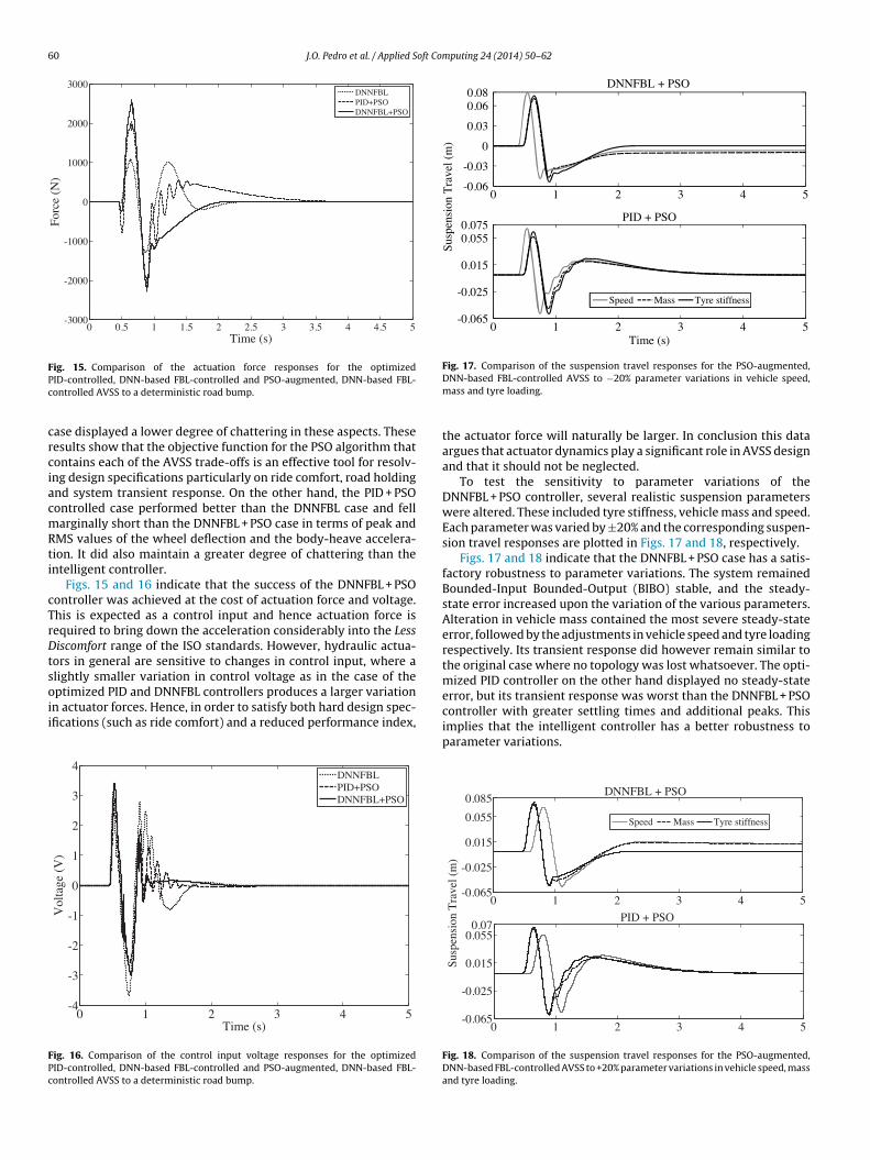
Figs. 15 and 16 indicate that the success of the DNNFBL + PSOontroller was achieved at the cost of actuation force and voltage.his is expected as a control input and hence actuation force isequired to bring down the acceleration considerably into the Lessiscomfort range of the ISO standards. However, hydraulic actua-

ors in general are sensitive to changes in control input, where alightly smaller variation in control voltage as in the case of the

ptimized PID and DNNFBL controllers produces a larger variationn actuator forces. Hence, in order to satisfy both hard design spec-fications (such as ride comfort) and a reduced performance index,

0 1 2 3 4 5-4

-3

-2

-1

0

1

2

3

4

Time (s)

Vol

tage

(V

)

DNNFBLPID+PS ODNNFBL+PS O

ig. 16. Comparison of the control input voltage responses for the optimizedID-controlled, DNN-based FBL-controlled and PSO-augmented, DNN-based FBL-ontrolled AVSS to a deterministic road bump.

DNN-based FBL-controlled AVSS to −20% parameter variations in vehicle speed,mass and tyre loading.

the actuator force will naturally be larger. In conclusion this dataargues that actuator dynamics play a significant role in AVSS designand that it should not be neglected.

To test the sensitivity to parameter variations of theDNNFBL + PSO controller, several realistic suspension parameterswere altered. These included tyre stiffness, vehicle mass and speed.Each parameter was varied by ±20% and the corresponding suspen-sion travel responses are plotted in Figs. 17 and 18, respectively.

Figs. 17 and 18 indicate that the DNNFBL + PSO case has a satis-factory robustness to parameter variations. The system remainedBounded-Input Bounded-Output (BIBO) stable, and the steady-state error increased upon the variation of the various parameters.Alteration in vehicle mass contained the most severe steady-stateerror, followed by the adjustments in vehicle speed and tyre loadingrespectively. Its transient response did however remain similar tothe original case where no topology was lost whatsoever. The opti-mized PID controller on the other hand displayed no steady-stateerror, but its transient response was worst than the DNNFBL + PSOcontroller with greater settling times and additional peaks. This

implies that the intelligent controller has a better robustness toparameter variations.

0 1 2 3 4 5-0.065

-0.025

0.015

0.055

0.085

Susp

ensi

on T

rave

l (m

)

DNNFBL + PS O

Speed Mass Tyre stiffness

0 1 2 3 4 5-0.065

-0.025

0.015

0.0550.07

PID + PS O

Fig. 18. Comparison of the suspension travel responses for the PSO-augmented,DNN-based FBL-controlled AVSS to +20% parameter variations in vehicle speed, massand tyre loading.

J.O. Pedro et al. / Applied Soft Computing 24 (2014) 50–62 61

0 1 2 3 4 5-0.05

-0.04

-0.03

-0.02

-0.01

0

0.01

0.02

0.03

0.04

Time (s)

Roa

d Pr

ofil

e (m

)

csD

gbr

dhdhfAgMl

sfstor

100

101

102

10-8

10-6

10-4

10-2

100

102

Frequency (Hz)

Pow

er R

atio

PassivePID+PS ODNNFBL+PS O

Fig. 21. Body-heave acceleration frequency response comparison of the proposedcontrol methods.

Table 6Frequency domain PSD settings.

Parameter Setting

Computation Algorithm WelchWindowing function HanningNumber of points included in fourier transform (NNFT) 1024Length of window (NWind) 256

Fig. 19. Random road profile.

The robustness of the proposed controller was also tested for thease of a random road disturbance presented in Fig. 19. The suspen-ion travel responses for the optimized PID and PSO-augmentedNNFBL subjected to this disturbance is presented in Fig. 20.

The optimized PID case reported larger peaks with a marginallyreater RMS value. This implies that the DNNFBL + PSO performedetter in this aspect as well, which further highlights its improvedobustness.

System sensitivity is also investigated through frequencyomain plots. The most sensitive frequencies of vibrations foruman exposure range between 2 and 80 Hz [43]. These stan-ards also explain that body-heave acceleration is used to quantifyuman exposure and hence body-heave acceleration under these

requencies is investigated. The frequency response of the proposedVSS schemes covering this range is presented in Fig. 21 and it wasenerated using the Power-Spectral-Density (PSD) estimates fromatlab signal processing toolbox. The settings for this estimate are

isted in Table 6.In this frequency range, the DNNFBL + PSO controller showed

ubstantially lower power ratios than its counterparts across mostrequencies. It maintained the best power ratio in the most sen-itive low frequency range. Beyond 10 Hz it performed worst than

he PVSS, but the power ratios in this range for all the control meth-ds are effectively negligible. These results once again highlight theobustness of the DNNFBL + PSO controller.

0 1 2 3 4 5-0.1

-0.05

0

0.05

0.1

0.15

Susp

ensi

on T

rave

l (m

)

Time (s)

PID+PSODNNFBL+PS O

Fig. 20. Suspension travel response subject to a random road disturbance.

Sampling frequency 80 Hz

Conclusion and future work

In light of the preceding discussion, the following conclusionsare made. Firstly, the DNN was successful in learning the dynam-ics of the AVSS. However, the DNNFBL-controlled case producedweaker data than the benchmark PID controller as it proved rathertedious to tune. PSO overcame this tuning issue and producedsignificantly better results which completely outperformed theoptimized PID-controlled case. The DNNFBL + PSO controlled caseis characterized with improved ride comfort, road holding, suspen-sion travel, settling time and contained a significantly lower degreeof chattering as compared to the optimized PID-controlled case.

However, this success came at the price of increased actuationforce. This is required to further minimize the effects of the trans-mitted road disturbance and hence improve the suspension travelresponse, ride comfort, settling time and road holding properties.On the contrary, the control input voltage did not alter signifi-cantly for the various cases. This may be attributed to the nature ofthe hydraulic actuator, where small increments in voltage developlarge changes in force. Furthermore, the optimal intelligent con-troller displayed an acceptable sensitivity to parameter variations.

The DNNFBL + PSO control displayed the best robustness withthe most desirable response for variations in parameter values,even though it had the shortfall of steady-state error. It showedbetter response than its PID counterpart in the frequency domainas well as when subjected to a random road disturbance.

In relation to future work, it is worth stating that success of theproposed controller may be extended to a full-car model to resolveits associating trade-offs. This is necessary as full-car modelsare much more complex and realistic. Furthermore, experimentalvalidation should be carried out as real-world model contains addi-

tional complexities and introduces various issues that have beenignored in numerical simulations.

6 oft Co

R

[

[

[

[

[

[

[

[

[

[

[

[

[

[

[

[

[

[

[

[

[

[

[

[

[

[

[

[

[[

[

[

[

[

2 J.O. Pedro et al. / Applied S

eferences

[1] J.E.D. Ekoru, J.O. Pedro, Proportional-integral-derivative control of nonlinearhalf-car electro-hydraulic suspension systems, J. Zhejiang Univ. Sci. A 14 (6)(2013) 401–416.

[2] N. Yagiz, L. Sakman, Robust sliding mode control of a full vehicle without sus-pension gap loss, J. Vib. Control 11 (11) (2005) 1357–1374.

[3] J.W. Shi, X.W. Li, J.W. Zhang, Feedback linearization and sliding mode controlfor active hydropneumatic suspension of a special-purpose vehicle, Proc. Inst.Mech. Eng. D, J. Automob. Eng. 211 (April (3)) (2010) 171–181.

[4] C.M. Huang, J-Y. Yen, M-S. Chen, Adaptive nonlinear control of repulsive Maglevsuspension systems, Control Eng. Pract. 8 (December (12)) (2000) 1357–1367.

[5] J.S. Lin, C.-J. Huang, Nonlinear backstepping active suspension design appliedto a half-car model, Int. J. Veh. Dyn. Mobil. 42 (June (6)) (2004) 373–393.

[6] Y. Sam, K. Huda, Modelling and force tracking of hydraulic actuator for an activesuspension system, in: Proceedings of the IEEE International Conference onIndustrial Electronics and Applications (ICIEA 2006), Singapore, May, 2006, pp.1–6.

[7] A.J. Koshkouei, K.J. Burnham, Sliding mode controllers for active suspensions,in: Proceedings of the 17th IFAC World Congress: The International Federa-tion of Automatic Control (IFAC’08), COEX, Seoul, Korea, 6–11 July, 2008, pp.3416–3421.

[8] Y.Md. Sam, J.H.S. Osman, M.R.A. Ghani, A class of proportional-integral slidingmode control with application to active suspension system, Syst. Control Lett.51 (3–4) (2004) 217–223.

[9] A. Chamseddine, T. Raharijaona, H. Noura, Sliding mode control applied toactive suspension using nonlinear full vehicle and actuator dynamics, in:Proceedings of the 45th IEEE Conference on Decision and Control, San Diego,CA, USA, 13–15 December, 2006, pp. 3597–3602.

10] N. Yagiz, Y. Hacioglu, Backstepping control of a vehicle with active suspension,Control Eng. Pract. 16 (December 12) (2008) 1457–1467.

11] J.H. Crews, M.G. Mattson, G.D. Buckner, Multi-objective control optimizationfor semi-active vehicle suspensions, J. Sound Vib. 330 (23) (2011) 5502–5516.

12] R.J. Wai, J.D. Lee, K.L. Chuang, Real-time PID control strategy for Maglev trans-portation system via particle swarm optimization, IEEE Trans. Ind. Electron. 58(February (2)) (2011) 629–646.

13] J-S. Chiou, S-H. Tsai, M-T. Liu, A PSO-based adaptive fuzzy PID-controllers,Simul. Model. Pract. Theory 26 (August (1)) (2012) 49–59.

14] K. Rajeswari, P. Lakshmi, PSO tuned adaptive neuro-fuzzy controller for vehiclesuspension systems, J. Adv. Inform. Technol. 3 (February (1)) (2012) 57–63.

15] C. Tang, G. Zhaq, H. Li, S. Zhuo, Research on suspension system based ongenetic algorithm and neural network control, in: Proceedings of the 2ndInternational Conference on Intelligent Computation Technology and Automa-tion Volume (ICICTA’09), vol. 1, Changsha, Hunan, 16th October, 2009, pp.468–471.

16] I. Eski, S. Yildirim, Vibration control of vehicle active suspension system usinga new robust neural network control system, Simul. Model. Pract. Theory 17(May (5)) (2009) 778–793.

17] A. Alfi, M.M. Fateh, Identification of nonlinear systems using modified particleswarm optimization: a hydraulic suspension system, Int. J. Veh. Dyn. Mobil. 49(June (6)) (2011) 871–887.

18] A.A. Aldair, W.J. Wang, Neural controller based full vehicle nonlinear activesuspension systems with hydraulic actuators, Int. J. Control Autom. 4 (June (2))(2011) 79–94.

19] R. Guclu, K. Gulez, Neural network control of seat vibrations of a non-linearfull vehicle model using PMSM, Math. Comput. Model. 47 (December (11–12))(2008) 1356–1371.

20] J.O. Pedro, O.A. Dahunsi, Neural network-based feedback linearization controlof a servo-hydraulic vehicle suspension system, Int. J. Appl. Math. Comput. Sci.21 (January (1)) (2011) 137–147.

21] J.O. Pedro, O.A. Dahunsi, N. Baloyi, Direct adaptive neural control of a quarter-car active suspension system, in: Proceedings of the 10th International Control

[

mputing 24 (2014) 50–62

Conference (AFRICON 2011), Livingstone, Zambia, 13–15 September, 2011,pp. 1–6.

22] M. Zapateiro, N. Luo, J. Vehl, Vibration control of a class of semi-active suspen-sion system using neural network and backstepping techniques, Mech. Syst.Signal Process. 23 (1) (2009) 1946–1953.

23] S. Yildirim, Vibration control of suspension system using a proposed neuralnetwork, J. Sound Vib. 277 (November (4–5)) (2004) 1059–1069.

24] J. Lin, R-J. Lian, C-N. Huan, W-T. Sie, Enhanced fuzzy sliding mode controller foractive suspension systems, Mechatronics 19 (July (7)) (2009) 1178–1190.

25] R.K. Pekgökgöz, M.A. Gürel, M. Bilgehan, M. Kisa, Active suspension of cars usingfuzzy logic controller optimized by genetic algorithm, Int. J. Eng. Appl. Sci. 2 (4)(2010) 27–37.

26] R.J. Lian, Enhanced adaptive self-organizing fuzzy sliding-mode controller foractive suspension systems, IEEE Trans. Ind. Electron. 60 (3) (2013) 958–968.

27] R. Guclu, K. Gulez, Neural network control of non-linear full vehicle modelvibrations, in: M. Lallart (Ed.), Vibration Control, 2010, ISBN: 978-953-307-117-6, InTech, Available from: http://www.intechopen.com/books/vibration-control/neural-network-control-of-non-linear-full-vehicle-model-vibrations

28] J. Deng, V.M. Becerra, R. Stobart, S. Zhong, Real-time application of a constrainedpredictive controller based on dynamic neural networks with feedback linear-ization, in: Proceedings of the 18th IFAC World Congress, Milano, Italy, August28–September 2, 2011, pp. 6727–6732.

29] J. Deng, V.M. Becerra, R. Stobart, Input constraints handling in an MPC/feedbacklinearization scheme, Int. J. Appl. Math. Comput. Sci. 19 (February (2)) (2009)219–232.

30] F.R. Garces, V.M. Becerra, C. Kambhampati, K. Warwick, Strategies for FeedbackLinearization: A Dynamic Neural Network Approach, 1st ed., Springer, 2003.

31] M.M. Gupta, L. Jin, N. Homma, Static and Dynamic Neural Networks: From Fun-damentals to Advanced Theory, John Wiley & Sons, Inc., Hoboken, NJ, USA,2003.

32] M. Norgaard, O. Ravn, N.K. Poulsen, L.K. Hansen, Neural Networks for Modellingand Control of Dynamic Systems, Springer, London, 2000.

33] H. Metered, P. Bonello, S.O. Oyadiji, An investigation into the use of neuralnetworks for the semi-active control of a magnetorheologically damped vehiclesuspension, Proc. Inst. Mech. Eng. D, J. Automob. Eng. 224 (July (7)) (2010)829–848.

34] Y. Becerikli, A.F. Konar, T. Samad, Intelligent optimal control with dynamicneural networks, Neural Netw. 16 (February (2)) (2003) 251–259.

35] R.K. Al-Seyab, Y. Cao, Differential recurrent neural network based predictivecontrol, Comput. Chem. Eng. 32 (July (7)) (2008) 1533–1545.

36] K. Nanayakkarra, Y. Ikegami, H. Uehara, Evolutionary design of dynamic neu-ral networks for evaporator control, Int. J. Refrig. 25 (September (6)) (2002)813–826.

37] L. Tian, C. Collins, A dynamic recurrent neural network-based controller for arigid-flexible manipulator system, Mechatronics 14 (June (5)) (2004) 471–490.

38] H.E. Merrit, Hydraulic Control Systems, John Wiley & Sons, New York, 1967.39] M. Jelali, A. Kroll, Hydraulic Servo-systems: Modelling, Identification and Con-

trol, Springer-Verlag, London, 2004.40] I. Fialho, G.J. Balas, Road adaptive suspension using linear parameter-varying

gain-scheduling, IEEE Trans. Control Syst. Technol. 10 (January (1)) (2002)43–54.

41] P. Gaspar, I. Szaszi, J. Bokor, Active suspension design using linear parametervarying control, Int. J. Veh. Auton. Syst. 1 (June (2)) (2003) 206–221.

42] O.A. Dahunsi, J.O. Pedro, O.T.C. Nyandoro, System identification and neuralnetwork-based PID control of servo hydraulic vehicle suspension system, SAIEEAfr. Res. J. 101 (September (3)) (2010) 93–105.

43] ISO2631, Mechanical Vibration and Shock – Evaluation of Human Exposure to

Whole-Body Vibration – Part 1: General Requirements, International Organi-zation for Standardization, Geneva, Switzerland, 2003.

44] J. Kennedy, R.C. Eberhart, Particle swarm optimization, in: Proceedings of the6th IEEE International Conference on Neural Networks, Perth, Australia, 27November–1 December, 1995, pp. 1942–1948.