Embed Size (px)
Citation preview

Intelligent Recommendation Engine
Dissertation
submitted in partial fulfillment of the requirementsfor the degree of
Master of Technology, Computer Engineering
by
Santosh N. Kalamkar
Roll No: 121022006
under the guidance of
Prof. Y. V. Haribhakta
Department of Computer Engineering and Information TechnologyCollege of Engineering, Pune
Pune - 411005.
June 2012

Dedicated tomy mother
Smt. Lata N. Kalamkar
andmy father
Shri. Nanabhau B. Kalamkar
for their love, endless supportand encouragement
DEPARTMENT OF COMPUTER
ENGINEERING AND
INFORMATION TECHNOLOGY,
COLLEGE OF ENGINEERING, PUNE
CERTIFICATE
This is to certify that the dissertation titled
Intelligent Recommendation Engine
has been successfully completed
By
Santosh N. Kalamkar(121022006)
and is approved for the degree of
Master of Technology, Computer Engineering.
Prof. Y. V. Haribhakta, Dr. Jibi Abraham,Guide, Head,Department of Computer Engineering Department of Computer Engineeringand Information Technology, and Information Technology,College of Engineering, Pune, College of Engineering, Pune,Shivaji Nagar, Pune-411005. Shivaji Nagar, Pune-411005.
Date :

Abstract
It has been observed that the growth of the amount of the data on Internet isexponential. The number of pages available on web is at least 8.87 billion and al-most another 1.5 million are being added daily. Retrieval of those documents willbe more efficient if the data is properly organized, and organization of data solelydepends on category of the document it belongs to. So, deciding the category ofthe text document is considered as an important aspect in the field of informationretrieval. In text categorization, feature extraction is one of the major strategiesthat aim at making text classifiers more efficient and accurate. We propose an ef-ficient entity extraction approach for feature extraction which contributes towardsaccurate text categorization. These extracted features are nothing but the contex-tual features of the text document such as protagonist, temporality, spatiality andorganization names. Once the contextual features are extracted, we are focusingon annotation of these entities with some unique parameter throughout the cor-pus. After annotation we used three measures for feature selection, namely, termfrequency (TF), information gain (IG) and chi-square (χ2). The experimentationis performed on standard benchmarking datasets such as NFS Abstract datasetsand Reuters-21578. The experimental results predict that the accuracy of text cat-egorization using the annotated features is better for NFS Abstract-Title datasetas compared to non-annotated features.
We have designed Contextual Probabilistic Model. This model works based onthe probabilistic theory along with the contextual features of the text documentand is intended to classify the given text document with the help of contextualfeatures that we have considered for extraction. To give the applicability of the textcategorization, we have designed an application “Research Paper RecommendationEngine”. This application functions on top of the contextual probabilistic model.This model accepts user suggested preferences as input, based on which we havedesigned a ruleset. Recommendation engine gives recommendations to user basedon ruleset and his/her contextual information.
iii

Acknowledgments
I have taken efforts in this project. However, it would not have been possible
without the kind support of Prof. Y. V. Haribhakta, who was abundantly
helpful and offered invaluable assistance and guidance. I consider myself very for-
tunate for being able to work with a very considerate and encouraging professor
like her. Deepest gratitude are also due to the members of the supervisory com-
mittee, Prof. V. K. Pachghare, Prof. V. Attar, Dr. J. V. Aghav and Dr.
Jibi Abraham.
I owe many thanks to my classmate and all of my friends for their unconditional
love, support, encouragement and assistance throughout the duration of project.
They always help me in exchanging any ideas and give the enjoyable studying
environment. They made my life at COEP a truly memorable experience and
their friendships are invaluable to me.
Santosh N. Kalamkar
College of Engineering, Pune
June 11, 2012
iv

Contents
Abstract iii
Acknowledgments iv
List of Figures vii
List of Tables viii
1 Introduction 1
1.1 Overview . . . . . . . . . . . . . . . . . . . . . . . . . . . . . . . . . 1
1.2 Text Categorization(TC) . . . . . . . . . . . . . . . . . . . . . . . . 2
1.3 Approaches for Text Categorization . . . . . . . . . . . . . . . . . . 2
1.3.1 Manual TC . . . . . . . . . . . . . . . . . . . . . . . . . . . 2
1.3.2 Automatic TC . . . . . . . . . . . . . . . . . . . . . . . . . 3
1.4 Applications of Text Categorization . . . . . . . . . . . . . . . . . . 4
1.5 Thesis Outline . . . . . . . . . . . . . . . . . . . . . . . . . . . . . . 5
2 Literature Survey 6
3 Our Approach 10
3.1 Annotation . . . . . . . . . . . . . . . . . . . . . . . . . . . . . . . 11
3.2 GATE . . . . . . . . . . . . . . . . . . . . . . . . . . . . . . . . . . 14
3.2.1 JAPE Rules . . . . . . . . . . . . . . . . . . . . . . . . . . . 14
3.3 Preprocessing . . . . . . . . . . . . . . . . . . . . . . . . . . . . . . 16
3.4 Contextual Probabilistic Model . . . . . . . . . . . . . . . . . . . . 18
3.5 Intelligent Recommendation Engine . . . . . . . . . . . . . . . . . . 21

4 Experiments and Results 27
4.1 Classifier and Datasets Used . . . . . . . . . . . . . . . . . . . . . . 27
4.2 System Specifications . . . . . . . . . . . . . . . . . . . . . . . . . . 28
4.3 Dataset Preparation . . . . . . . . . . . . . . . . . . . . . . . . . . 28
4.4 Feature Selection Methods . . . . . . . . . . . . . . . . . . . . . . . 28
4.4.1 Term-Frequency (TF) . . . . . . . . . . . . . . . . . . . . . 29
4.4.2 CHI-Square (χ2) . . . . . . . . . . . . . . . . . . . . . . . . 29
4.4.3 Information gain (IG) . . . . . . . . . . . . . . . . . . . . . 30
4.5 Measures of categorisation effectiveness . . . . . . . . . . . . . . . . 30
4.5.1 Precision . . . . . . . . . . . . . . . . . . . . . . . . . . . . . 31
4.5.2 Recall . . . . . . . . . . . . . . . . . . . . . . . . . . . . . . 31
4.5.3 F-Measure . . . . . . . . . . . . . . . . . . . . . . . . . . . . 31
4.6 Performance Analysis . . . . . . . . . . . . . . . . . . . . . . . . . . 32
4.7 Results of Recommendation Engine . . . . . . . . . . . . . . . . . . 37
5 Conclusion and Future Work 40
5.1 Conclusion . . . . . . . . . . . . . . . . . . . . . . . . . . . . . . . . 40
5.2 Future Work . . . . . . . . . . . . . . . . . . . . . . . . . . . . . . . 41
A Publications 42
A.1 Feature Annotation for Text Categorization . . . . . . . . . . . . . 42
Bibliography 43
vi

List of Figures
1.1 Basic Categirization System . . . . . . . . . . . . . . . . . . . . . . 2
1.2 Decision matrix for training set and test set . . . . . . . . . . . . . 4
3.1 Proposed System Design . . . . . . . . . . . . . . . . . . . . . . . . 10
3.2 Rich context information on cricket news [34] . . . . . . . . . . . . 12
3.3 Highlighted four dimensions on real time Cricket news . . . . . . . . 13
3.4 After annotating all four dimensions . . . . . . . . . . . . . . . . . 14
4.1 Performance for different classifiers using Information Gain for NFS
Abstract-Title dataset . . . . . . . . . . . . . . . . . . . . . . . . . 32
4.2 Performance for different classifiers using Term Frequency for NFS
Abstract-Title dataset . . . . . . . . . . . . . . . . . . . . . . . . . 33
4.3 Performance for different classifiers using Chi-Square for NFS Abstract-
Title dataset . . . . . . . . . . . . . . . . . . . . . . . . . . . . . . . 33
4.4 Performance for different classifiers using term frequency for Reuters-
21578 . . . . . . . . . . . . . . . . . . . . . . . . . . . . . . . . . . . 34

List of Tables
3.1 List of sample features extracted for annotation . . . . . . . . . . . 16
3.2 Domain Rating based Ruleset . . . . . . . . . . . . . . . . . . . . . 24
3.3 Level Rating based Ruleset . . . . . . . . . . . . . . . . . . . . . . . 26
4.1 The contingency table for category ci . . . . . . . . . . . . . . . . . 30
4.2 The global contingency table . . . . . . . . . . . . . . . . . . . . . . 31
4.3 F-Measure for real time Cricket dataset . . . . . . . . . . . . . . . . 35
4.4 F-Measure for Reuters-21578 dataset . . . . . . . . . . . . . . . . . 35
4.5 F-Measure for NFS Abstract dataset . . . . . . . . . . . . . . . . . 36
viii

Chapter 1
Introduction
1.1 Overview
The data in digital form is increasing day by day due to the increasing nature
of internet. It has been observed that the growth of the amount of the data on
internet is exponential. The number of pages available on web is at least 8.87
billion [16] and almost another 1.5 million are being added daily. Around 70-80%
of the data on Internet is in unstructured format [18] and is growing 10-50x more
than structured data. Unstructured data does not have a pre-defined data model
and also, does not fit well into relational tables. Unstructured data is typically
text-heavy, but may contain data such as numbers, temporal information, spatial
information, protagonist and/or dates. This results in ambiguities and irregulari-
ties that make it difficult to understand using our traditional computer program
[18] as compared to relational databases. The management of unstructured data
is considered as one of the most difficult issues in the field of computer science, the
main reason being that the techniques, tools and algorithms that have proved so
successful transforming structured data into business intelligence and actionable
information simply don’t work when it comes to unstructured data.
In information retrieval, retrieval of those unstructured documents will be more
efficient if the data is properly organized, and organization of data solely depends
on category of the document it belongs to. Deciding the category of each document
1

1.2 Text Categorization(TC)
manually has become more effort-consuming and also requires skilled labors.
1.2 Text Categorization(TC)
Text Categorization aims to automatically assign most suitable category labels
from the available predefined set of labels to the unseen documents.
Figure 1.1: Basic Categirization System
As shown in figure 1.1, D is a set of text documents d1, d2, d3..., dn. And, we
have different predefined categories (class labels) such as c1, c2, c3..., cm. Catego-
rizer or classifier is a function (K) which maps a document from set D to one or
more categories in set C.
1.3 Approaches for Text Categorization
1.3.1 Manual TC
Different approaches are used for classifying text documents, such as, manual
classification and automatic text classification. In manual categorization, decid-
ing whether a documentd should be categorized under category c requires, to
some extent, an understanding of the meaning of both d and c. This is clearly
unsatisfactory since:
1. The categorization of any significant portion of the Web requires too much
skilled man power.
2

1.3 Approaches for Text Categorization
2. Manual categorization is too slow to keep a catalogue up to date with the
evolution of the Web. New documents are published, old ones are either
removed or updated, new categories emerge, old ones fade away or take up
new meanings. Doing all above activities manually is practically impossible.
3. More efforts and time consuming process.
4. Manual categorization does not guarantee in itself the quality of the resulting
catalog, since categorization decisions are always highly subjective.
1.3.2 Automatic TC
In the ‘80s, different approaches used for construction of automatic document
categorizers, includes knowledge-Engineering them, i.e. manually building an ex-
pert system capable of taking categorization decisions. Such an expert systems
are considered of a set of manually defined rules (one per category) of type if
< DNF Boolean formula > then < category >, i.e. if the document satisfies
< DNF Boolean formula > (DNF standing for ‘disjunctive normal form’) then
categorize under < category >. The main drawback of “manual” approach of the
construction of automatic classifiers is knowledge acquisition bottleneck.
In early ‘90s, a new approach to the construction of automatic document clas-
sifiers gained prominence and eventually became the dominant one is machine
learning approach. In the machine learning approach a general inductive process
automatically builds a classifier for a category Ci by observing the characteris-
tics of a set of documents that have previously been classified under category Ci
manually by domain experts; with the help of these characteristics, the inductive
process gleans the characteristics that a novel document should have in order to
be categorized under Ci.
The machine learning approach relies on the existence of a an initial corpus
D = {d1, d2, ..., ds} of documents that have been previously categorized under the
3

1.4 Applications of Text Categorization
same set of categories C = {c1, c2, ..., cm}. This means that corpus comes with a
correct decision matrix.
Figure 1.2: Decision matrix for training set and test set
The value of 1 for caij is interpreted as an indication from the experts to file
dj under class ci, while a value of 0 for is interpreted as an indication from the
expert not to file dj under ci. For evaluation purposes, in the first stage of classifier
construction the initial corpus is typically divided into two sets, not necessary of
equal size:
• a training set Tr = {d1, d2, ..., dg}. This is the set of example documents
used for training the classifier by inducing document characteristics.
• a testing set Te = {dg+1, dg+2, ..., ds}. This set will be used for the purpose
of testing the effectiveness of the induced classifier.
1.4 Applications of Text Categorization
Categorization of text documents in an organized manner is a requirement of many
real world applications, such as:
• Library Science
• Information Science
• Computer Science
These applications provide a conceptual view of document collections. For exam-
ple, academic data is often classified in technical and non-technical domains; in
4

1.5 Thesis Outline
medical science patient reports are often indexed from multiple aspects by using
taxonomies of disease categories, types of surgical procedures and so on. There-
fore, automated text categorization (TC) has become more challenging task in the
field of information retrieval. The intellectual classifications of documents have
mostly been the subject of library science, while the algorithmic classifications of
documents have mostly been done in information science and computer science.
1.5 Thesis Outline
The rest of the thesis is organized as follows: In Section 2 we give a brief description
of the important papers that we have studied or utilized as a part of our literature
survey. In Section 3, we introduce our proposed system model and details of each
part. Section 4 shows the experimental results achieved so far and remainder of
the thesis presents the conclusion and future work.
5

Chapter 2
Literature Survey
In Machine Learning and Statistics, feature selection for classification is also known
as attribute selection or variable subset selection. While choosing subset of feature
we try to remove most irrelevant and redundant features from the available feature
set. We know that optimal feature space selection for supervised learning methods
requires an exhaustive search of all possible subsets of available feature space.
Subset selection algorithms can be further classified into three main types,
namely, Wrapper approach, Filter approach and Embedded approach [2, 9, 10].
In wrapper approach search algorithms are used to search features from available
feature space and evaluate each subset by running a model on subset. Filter ap-
proach works similar as wrapper for searching the subset of feature space, but,
instead of evaluating against a model, a simpler filter is evaluated. And, it has
been observed that wrapper approaches outperforms filter approaches [10]. Em-
bedded techniques are generally embedded in and are specific to a model. There
are numerous feature selection methods, statistic based ones are term frequency
(TF), Term frequency-Inverse document frequency (TF-IDF), Chi-Square (χ2),
Information Gain (IG), Document Frequency (DF) and Mutual Information (MI).
Term-Frequency is nothing but number of occurrences of a term in particular doc-
ument. Terms with high TF are considered to be of more relevance or importance
for that document. Information Gain focuses on presence and absence of a term in
a document for feature selection. Degree of goodness between term and particular
6

category is measured with the help of the Chi-Square statistic. Features having
high dependency on category are selected in this method. Document Frequency
refers to the number of document containing that feature. All above mentioned
feature selection methods are ultimately aimed to increase the classification accu-
racy.
Stephanie Chua and Narayanan [3] exploited semantic relatedness between terms
for feature selection. WordNet [17], a lexical database, is used to exploit the noun
synonyms and word senses for selecting features that are semantically much related
to a category of a document. If terms with overlapping word senses co-occurred
in a category are considered as features and are considered to be significant terms
to represent a category. Yi Guo et al. [5] extracted different dimensions from text
document and are used to build cognitive situation vectors. In their approach each
document along with their reference document of a predefined category is repre-
sented with a matrix of situation vectors, and each vector consists of six different
dimensions. Semantic relation of situation dimensions, correlation of cognitive
situation vectors are used to classify the text document.
Zi-Jun Yu et al. [1] proposed Keyword combination extraction based on ant
colony optimization (KCEACO) a novel algorithm, and is used to extract optimal
keyword combinations which in turn used to describe the category of the docu-
ment the keywords extracted from. In [11], a novel hybrid approach based on
ant colony optimization (ACO) and information gain (IG) for feature selection in
categorization. In some approaches [8], high performing features are selected for
classification. In [4], textual references (also called as ‘spots’) to named entities
are identified and annotating such spots with unambiguous entity IDs (called as
labels) for resolving ambiguity of the text document. Spots refer to the real world
entities from an entity catalog. But main focus of this entity annotation is text
data disambiguation. Wang Xiaoyue and Bai Rujiang [14] used ontologies and
natural language processing techniques for identifying semantic relationships be-
tween key terms. By using the same technique they represented “Bag of Concepts”
7

(BOC) with the help of traditional “Bag of Words” (BOW) matrix. In [8], they
used variant of the -co-occurence method for redundancy reduction, and it uses
filter feature selection methods. They combined top performing methods (such as
multiclass version of IG and CHI MAX) and observed potential performance gain
when combined together.
Francois Paradis et. al [19] presented a new approach for the classification of
‘noisy’ documents with the help of bigram and named entities. The approach
combines conventional feature selection with a contextual approach to filter out
passages around selected features. Two levels of passage filtering are considered:
sentences or windows (i.e. sequence of words). Tan, Wang, and Lee [20] find
an improvement on the classification of Web pages, by using a combination of
bigrams and unigrams selected on the merits of their InfoGain score. However
the same technique applied to the Reuters collection did not yield the same gain,
mostly because of its over-emphasis on ‘common concepts’. Since their method
favours recall, the authors conclude it was harder to improve Reuters because
it already had high recall. Pang et al. [21] used syntactic (unigrams, bigrams,
unigrams + POS, adjectives, and unigrams + positions), limited consideration to
unigrams appearing at least four times in their 1400-document corpus, and the
bigram occurring most often in the same dataset (the selected bigram all occurred
at least seven times). Yu and Hatzivassiloglou [22] used words, bigrams, and
trigrams, as well as the parts of speech as features in each sentence.
Text classification is often used in the process of named entity extraction [23]
but rarely the other way around. Its use in classification is mostly restricted to
replacing common strings such as dates or money amounts with tokens, to increase
the ability of the classifier to generalise.
FIS(Feature and Instance Selection) [24] approach is focused on combining both
feature selection and instance selection approaches. Their approach shows that,
FIS considerably reduces both the number of features and the number of instances.
John et. al [25] identify three types of features: Irrelevant features, which can be
8

ignored without degrading the classifier performance, strongly relevant features
that contains useful information such that if removed the classification accuracy
will degrade and weakly relevant features that contain information useful for the
classification.
9

Chapter 3
Our Approach
In our approach we are focusing on contextual features of the text for classifica-
tion. Figure 3.1 shows the proposed system design of our approach. System has
four main modules: Annotation, Preprocessing module, Contextual Probabilistic
Model (CPM) and Recommendation engine (IRE). This chapter explains each of
the modules of the proposed system in detail.
Figure 3.1: Proposed System Design
10

3.1 Annotation
3.1 Annotation
Text data is associated with rich context information, which refers to the situations
in which the text was originally produced. There are different taxonomies of
context from different disciplines. For example, the linguistic context, or the verbal
context is commonly used in linguistics which refers to the local surrounding text
of a linguistic unit that is useful for inferring the meaning of the linguistic unit [33].
Social context, on the other hand, is a key concept used in sociology which refers to
the social variables that influence the use of language of a social identity (e.g., an
author. A more general notion of context is known as the situational context, or
context of situation, which is first proposed by the Polish anthropologist Bronislaw
Malinowski and then formalized with linguistic theory by J. R. Firth [26, 27]. It
is concerned with the evaluable conditions or situations in which the text content
is produced, including the situations that are either environmental or personal.
Such contextual information can be either explicit or implicit. Explicit con-
textual information can be time and the location where a blog article is written
and the author(s) of different publications. Implicit contextual information can be
positive or negative sentiment that an author had when he/she wrote a product
review. There may be complex context such as social network of the users.
In many real world applications of text mining, we can see that various context
information can serve as an important guidance for understanding, analyzing, and
mining the text data. For example, temporal patterns of book discussions in blogs
(e.g., spikes of discussions) have shown to be useful to predict books sales [28].
Author-topic patterns can facilitate the finding of experts and the understanding
of the research communities [32]. Analyzing contextual patterns in search logs
can help a search engine company to better serve its customers by re-organizing
the search results according to the contexts of a new query [30]. Analyzing the
bursts and decays of topics in scientific literature would enable researchers to
better organize, summarize, and digest the historical literature and to discover and
envision new research trends [29]. Analyzing the sentiments in customer reviews
11

3.1 Annotation
is helpful in summarizing public opinions about products and social events [31].
Figure 3.2: Rich context information on cricket news [34]
Figure 3.2 is a random snapshot from “www.icc-cricket.yahoo.net” website. It
is interesting to see how many types of context information exist in such a short
piece of text. Contextual information includes ‘name of the person’, ‘location’,
‘organization’ and ‘date’.
We have considered four different context for mining the text data i.e. di-
mensions [5] such as protagonist, temporality, spatiality and organization names.
These dimensions are considered as important contextual features in a text docu-
ment.
Annotation is a process of extracting such contextual features from text doc-
ument and annotating with unique single instance throughout the corpus. For
example, “Captain Mahendra Singh Dhoni” or simply “Mahendra Singh Dhoni”
is considered as a feature instead of considering separate terms like ‘Captain’,
12

3.1 Annotation
‘Mahendra’, ‘Singh’, ‘Dhoni’. We extracted four types of such dimensions from
text for annotation, and those are protagonist, spatiality, temporality and orga-
nizations. We used free and open source tool for extracting all such dimensions.
Annotation also helps in minimizing the loss of important information.
Protagonist denotes name of persons or actors in events, also Central character
of event.
Spatiality indicates spatial information or information about locations.
Temporality presents time or temporal information. It includes dates, infor-
mation about days in text, etc.
Organizations are the names of the organizations in textual document.
Figure 3.3: Highlighted four dimensions on real time Cricket news
Figure3.3 shows highlighted different dimensions (protagonist, spatiality, tem-
porality and organizations) that are extracted for annotation for real time cricket
news and Figure3.4 shows the same text data after annotation. These figures show
the conceptual view for the annotation.
13

3.2 GATE
Figure 3.4: After annotating all four dimensions
3.2 GATE
General Architecture for Text Engineering (GATE) [6] is a open source software,
and is developed at the University of Sheffield. GATE provides a number of useful
and easy-to-customise components, grouped together to form ANNIE - A Nearly-
New Information Extraction system. It (ANNIE) is a set of modules consisting
of a tokenizer, a gazetteer, a sentence splitter, a part of speech tagger (POS
Tagger), a named entities transducer and a co-reference tagger. We used ANNIE
plugin for text processing and to extract four dimensions as mentioned in previous
section. Current version of GATE is capable of handling languages like English,
Hindi, Spanish, Chinese, French, German, Arabic, Bulgarian, Italian, Cebuano,
Romanian, Russian.
It accepts input data in TXT, XML, HTML, PDF, Doc format. JAPE Trans-
ducers are used along with GATE for annotating text.
3.2.1 JAPE Rules
The JAPE (Java Annotation Pattern Engine) language allows users to customise
language processing components by creating and editing linguistic data (e.g.,
grammars, rule sets), while their efficient execution is automatically provided by
GATE. Once familiar with GATEs data model, users do not find it difficult to write
JAPE pattern-matching rules, because they are effectively regular expressions. An
14
3.2 GATE
example rule below shows a typical JAPE rule. The left-hand side describes pat-
terns of annotations that need to be matched, whereas the right-hand side specifies
annotations to be created as a result:
Rule: Company1
Priority: 25
(
({Token.orthography
== upperInitial})+
{Lookup.kind == companyDesignator}
):companyMatch
-->
:companyMatch.NamedEntity =
{kind = "company", rule = "Company1"}
The rule matches a pattern consisting of any kind of word (expressed as a Token
annotation, created by a previous text tokenisation module), which starts with an
upper-case letter, followed by a word which typically indicates companies, such as
‘Ltd.’ and ‘GmbH’ (the Lookup annotation). The entire match is then annotated
with entity type “NamedEntity”, and given a feature “kind” with value “company”
and another feature “rule” with value “Company1”. The “rule” feature is simply
used for debugging purposes, so it is clear which particular rule has fired to create
the annotation. For example, when this rule is applied to a document containing
“Hewlett Packard Ltd.”, the left-hand side will match, because there are two
tokens starting with a capital letter, followed by the company designator ‘Ltd.’.
Table 3.1 shows the sample dimensions that we extracted for real time cricket
dataset. Cricket dataset contains all four dimensions which we have considered
for extraction i.e. protagonist, spatiality, temporality and organizations.
15

3.3 Preprocessing
Table 3.1: List of sample features extracted for annotation
Dimension Features Extracted
Protagonist Captain William Porterfield, captain Mahela
Jayawardena, President Shashank Manohar,
Chairman Andrew Hilditch, Captain Sachin Ten-
dulkar, Sir Garfield Sobers, Sir Donald Bradman,
Mitchell Johnson, Ravindra Jadeja
Spatiality Chinnanwawamy Stadium, United Arab Emi-
rates, Providence Stadium, Western Australian,
Brabourne Stadium, DY Patil Stadium, The
Netherlands, Galle District
Temporality ‘Monday, April 28, 2008’, ‘September 14, 2009’,
next four years, tomorrow morning, ‘Sunday,
March 6’, last ten years, February 14-18, Wednes-
day, the 1970s
Organizations Maharashtra Tourism Development Corporation,
Western Australian Cricket Association, Interna-
tional Cricket Council, Sahara Adventure Sports
Group, Australian Associated Press
3.3 Preprocessing
Text document consists of thousands of terms and it has been observed that for
learning algorithms, it is very difficult to cope with such high term space. To over-
come this problem, preprocessing of the text document is necessary. Morphological
analysis [7] is the very first step that is applied on text in traditional preprocess-
ing, and covers three sub-processing tasks: tokenization, stemming, recognition of
ending of words. Morphology is a part of linguistic which is dealing with words.
TF considers the number of occurrences of a word in document, but in plain
English text non-semantic words [7] like articles, conjunctions, prepositions, pro-
nouns etc. are inevitable in usage. Also, because of their small vocabulary it
covers a significant part of text. Such non-semantic words are called as stopwords,
and are considered to be of less importance in classification. So, we removed such
16

3.3 Preprocessing
words before calculating TF and TF-IDF.
After removal of stopwords from text document the next task applied is word
stemming (also called as lemmatization). Stemming is intended to replace a word
by its base or root word. In this the words like agreed, agreeing, disagree, agree-
ment, and disagreement are replaced with a single word ‘agree’. Also, the variation
“Robert’s” in sentence is reduced to “Robert”. In some cases the result of stem-
ming may lead to an incorrect root. The stemming is still considered to be useful
[7] because same stem is generated for all other inflections of the root. Also,
stemming of the word increases precision and recall in information retrieval [7]
therefore stemming is considered as one of the major steps in preprocessing of
text document.
Following a selection of suffixes and prefixes for removal during stemming:
1. Suffixes: ly, ness, ion, ize, ant, ent, ic, al, ical, able, ance, ary, ate, ce, y,
dom, ed, ee, eer, ence, ency, ery, ess, ful, hood, ible, icity, ify, ing, ish, ism,
ist, istic, ity, ive, less, let, like, ment, ory, ty, ship, some, ure
2. Prefixes: anti, bi, co, contra, counter, de, di, dis, en, extra, in, inter, intra,
micro, mid, mini, multi, non, over, para, poly, post, pre, pro, re, semi, sub,
super, supra, sur, trans, tri, ultra, un
But, most of the stemming algorithms do not remove prefix of a term. The main
reason for this is the huge impact for the meaning of the sentence. For instance,
stemming of the word nonhazardous to hazardous is a parlous change.
WordNet based stemmer performs well as compared to statistical rule based
stemmers. So, stemming is performed with the help of WordNet stemmer.
17
3.4 Contextual Probabilistic Model
3.4 Contextual Probabilistic Model
As we have discussed in section 3.1, text data is rich of contextual information such
as protagonist- person names, temporal- time relevant information, spatiality- ge-
ographical locations and different entity names like organization and many others.
Contextual information helps in better understanding of the text data. Also,
contextual information is of particular importance for collections or corpora com-
posed of samples from a variety of different kinds of text.
Hui Wang and Sally McClean [35] have introduced a principled approach that
utilises a novel definition of contextual probability which they have termed as G-
Contextual Probability Function. They have used all the sets that overlap with
the set for which they want to calculate the probability. Ultimately, they have
tried to include information from all possible neighbourhood. Ernandes et al. [36]
propose a term weighting algorithm that recognizes words as social networks and
enhances the default score of a word by using a context function that relates it to
neighbouring high scoring words. Their work has been suitably applied for single
word QA as demonstrated for crossword solving.
The earliest probabilistic model is known as probabilistic latent semantic anal-
ysis (PLSA) [38]. In the context of information retrieval, the model is also called
probabilistic latent semantic indexing (PLSI) [39]. The basic assumption of this
model is that there are k latent topics in the text collection, each of which is rep-
resented by a multinomial distribution of words. Mei et al. [37] extends the prob-
abilistic latent semantic analysis (PLSA) model by introducing context variables
for contextual document modelling. One approach of handling context informa-
tion in text is to treat the context information simply as additional observations
besides the words. In this way, one can construct a probabilistic model that not
only generates the content (i.e., words) in text, but also the context information.
For example, Li et al. [40] proposed a probabilistic model to detect retrospective
news events by explaining the generation of “four Ws” from each news article.
18

3.4 Contextual Probabilistic Model
Contextual Probabilistic Module is basically intended to classify the text docu-
ment based on the contextual information from the text itself. We have considered
four types of contexts for building contextual probabilistic model and those are
as mentioned above i.e. person names, time relevant information, geographical
locations and organization names.
A probability of a document d being in a class c is calculated as,
P (c/d) = P (c)∏
16k6n
P (tk/c) (3.1)
Where P (tk/c) is the conditional probability of term tk occurring in a document
of class c. Here interpretation of P (tk/c) is a measure of how much evidence tk
contributes that c is the correct class. P (c) is the prior of a class i.e. probability
of a document occurring in a class c.
W =< t1, t2, ..., tn > are the tokens in d it forms the vocabulary.
Where, |W | = n
As in text classification, our goal is to find the best class for the document. With
the help of Maximum Likelihood Estimation we find the most likely or Maximum
a posteriori (MAP) class cmap.
i.e.,
cmap = arg maxcεCP (c/d)
= arg maxcεCP (c)∏
16k6n
P (tk/c) (3.2)
Log-MAP can be calculated as,
cmap = arg maxcεC [ logP (c) +∑
16k6n
logP (tk/c) ] (3.3)
Estimation of parameters P (c) and P (tk/c), Here we are trying the maximum
likelihood estimation (MLE ), which is simply the relative frequency of term and
19

3.4 Contextual Probabilistic Model
Algorithm 1 Finding Maximum a Posteriori (MAP) class for a given documentwith Contextual Probabilistic approach
1: procedure FIND PRIORS LIKELIHOOD(C,D)/∗ This process extracts vocabulary from the training dataset and ∗//∗ calculates the priors for each document as well as the likeliho- ∗//∗ -od of each feature with respect to every class. ∗/
2: V = CALL ExtractVocabulary(D)/∗ Input to this process is annotated (annotation wrt four ∗//∗ contexts i.e. person names, geographical locations, dates ∗//∗ and organization names) text documents, Pre-process ∗//∗ the documents to remove noisy elements, such as ∗//∗ stop words and punctuations. ∗/
3: N = CALL CountDocuments(D)/∗ Count the total number of documents in training dataset. ∗/
4: for all c in C do5: Nc = CALL CountDocsInClass(D, c)6: prior[c] = Nc/N7: textc = CALL CombineTextOfAllDocsInClass(D, c)8: for all t in V do9: Tct = CALL CountTokensOfTerm(Tct, t)10: end for11: for all t in V do12: condprob[t][c] = (Tct + 1)/
∑t′ Tct′
13: end for14: end for15: return V , prior, condprob16: end procedure
17: procedure Calculate MAP(C, V , prior, condprob, d)18: W = CALL ExtractContextualFeatures(V ,d)19: for all c in C do20: score[c] = prior[c]21: for all t in W do22: score[c]∗=condprob[t][c]23: end for24: end for25: return arg maxcεCscore[c]26: end procedure
20

3.5 Intelligent Recommendation Engine
corresponds to the most likely value of each parameter given the training data.
Priors estimation is done as follows:
P (c) =Nc
N(3.4)
Where, Nc = number of documents in class c
N = total number of documents
And, we estimate conditional probability P (tk/c) as follows:
P (t/c) =Tct
(∑
t′εV Tct′)(3.5)
Where, tk/c is number of occurrences of t in training documents from class c.
For test document we extract the contextual features from the document and
with the help of their likelihood for the particular class and the prior of the doc-
ument, we calculate the Maximum a posteriori (MAP) for that document by
formula (3.3). Algorithm 1 explains the contextual probabilistic model in detail.
3.5 Intelligent Recommendation Engine
Intelligent Recommendation Engine functions on top of the Contextual Proba-
bilistic Model. Once the classification is done we can make use of this classified
data effectively. Intelligent Recommendation Engine gives the applicability of the
text categorization system.
Aim of this Recommendation Engine is to recommend “Research Papers” to the
users. This model accepts user suggested preferences such as interest area of user,
interest rating for the interest area, his/her qualification etc. as input, based on
21

3.5 Intelligent Recommendation Engine
which we have designed and implemented corresponding ruleset. This ruleset in
turn will be used by the model for recommending the closer matches to the user.
For designing the recommendation engine, we have considered three different
profiles, as:
• User Profile
• Paper Profile
• Suggestion Profile
The structure for each of the above profiles is shown below:
User Profile:
<user number= 1>
<name> Santosh Kalamkar </name>
<edu. qualification> Masters of Technology </edu. qualification>
<interest area= 1> NLP </interest area>
<rating> 3 </rating>
<keywords> text categorization </keywords>
<interest area=2> networking </interest area>
<rating> 2 </rating>
<keywords> packet routing </keywords>
<interest area=3> network security </interest area>
<rating> 2 </rating>
<keywords> encryption algo </keywords>
</user>
In user profile we are taking inputs from user, it includes, name of the user,
educational qualification, area of interest along with rating for that area and key-
words. This information in turn used for recommending papers to the user.
22

3.5 Intelligent Recommendation Engine
Paper Profile:
<paper number 1>
<title> Feature Annotation for Text Categorization </title>
<authors> S. Kalamkar, Y. Haribhakta </authors>
<avg. rating> 4.2 </avg. rating>
<keywords> categorization, annotation, context </keywords>
</paper>
<paper number 2>
<title> SVM-based multi-class classifier </title>
<authors> Y. Liu, Zhisheng You, LipingCao </authors>
<avg. rating> 3.42 </avg. rating>
<keywords> SVM, muti-class classifier </keywords>
</paper>
Paper profile contains paper related information such as, title of the paper,
author names, keyword related to that paper and its average rating of that paper.
Recommendations are generated with the help of user profile and paper profile.
Suggestion Profile:
<user ID= snk1703>
<suggestion number=1>
<paper ID= P1>
<title> Feature Annotation for Text categorization </title>
<domain> Natural Language Processing </domain>
<avg. rating> 4.2 </avg. rating>
</suggestion>
<suggestion number=2>
<paper ID= P2>
<title> SVM-based multi-class classifier </title>
<domain> Natural Language Processing </domain>
<avg. rating> 3.42 </avg. rating>
23

3.5 Intelligent Recommendation Engine
</suggestion>
Suggestion profile is nothing but the recommendations to the user. It includes
different suggestions (i.e. papers) along with their id, title and average rating.
We have designed three different rulesets with the help of suggested preferences
by the user. The design of the rulesets is based on two main assumptions:
• If user rated his/her interest area low, recommend the only papers having
high average rating for that paper.
• If user rated his/her interest area high, recommend the papers having even
low average rating for that paper.
Based on the above two mentioned assumptions, three different rulesets are as
follows:
• ‘Domain Rating’ based ruleset
• ‘Educational qualification’ based ruleset
• ‘Keyword match’ based ruleset
In domain rating based ruleset, we calculate the average rating of the Research
paper. We recommend that paper to the user only if it belongs to the same domain
as that of the users interest and satisfies the rule from Table 3.2.
Table 3.2: Domain Rating based Ruleset
Users rating Papers average rating1 > 42 > 33 > 2.54 > 25 > 1.5
24

3.5 Intelligent Recommendation Engine
Rating based rules are as follows:
∀Pi ε user interest area
calc avg rating(Pi);
if(avg rating > 1.5 && interestarea rating == 5) addtolist(Pi);
else if(avg rating > 2 && interestarea rating == 4) addtolist(Pi);
else if(avg rating > 2.5 && interestarea rating == 3) addtolist(Pi);
else if(avg rating > 3 && interestarea rating == 2) addtolist(Pi);
else if(avg rating > 4 && interestarea rating == 1) addtolist(Pi);
Where, Pi is a paper Id, and
addtolist() is a function for adding paper to recommendation list.
For designing educational qualification based ruleset, we are taking inputs from
user for every previously recommended paper to the user under the title ‘Level
Rating’. This ruleset also considers the domain of the paper and users interest
domain before recommendations.
Level Rating based rules are as follows:
Some considerations- Edu.Qualification Equivalent no.
UG 1
PG 2
PhD 3
∀Pi ε user interest area
calc avg levelrating(Pi);
if(avg levelrating > 2 && user edu qualification == “PG′′)
addtolist(Pi);
else if(avg levelrating > 2.3 && user edu qualification == “PhD′′)
addtolist(Pi);
else if(avg levelrating > 1.5 && user edu qualification == “UG′′)
addtolist(Pi);
25

3.5 Intelligent Recommendation Engine
Here, avg levelrating() calculates papers level average rating.
Table 3.3: Level Rating based Ruleset
Users qualification Papers average level ratingUG > 1.5PG > 2PhD > 2.3
In keyword based ruleset, we consider the domain specific keyword matching
between users entered keyword set and papers keywords.
∀Pi ε user interest area
if(keywordmatch(Pi keyword, interest area keywords))
addtolist(Pi);
Here, Pi keywords-keywords related to paper
if Pi keywords matches interest area keywords, this paper is added to the rec-
ommendation list.
26

Chapter 4
Experiments and Results
4.1 Classifier and Datasets Used
We selected five high-performing classifiers for comparing the results of our prepro-
cessing with feature annotation approach and traditional preprocessing. Classifiers
selected include: Nave Bayes Multinomial (NBM), JRip, SVM (SMO), J48 and
Bagging. WEKA [13] provides an implementation of these five methods and we
have used default settings for each of those methods.
For experimentation we selected NFS Abstract [12] dataset and Reuters-21578
[15] dataset to evaluate the performance of classifiers based on our methods. Also,
we collected real time news related to sports and formed a new dataset. In sport,
specifically cricket, and in cricket four types of cricket that is being played, test
cricket, one day matches, IPL (Indian Premier Leagues T-20 matches), and world
cup matches. So, we selected four classes as IPL, TEST CRICKET, WORLD CUP,
and ODI. For each class we collected 200 documents. The result section shows
the results obtained with 10-fold cross-validation for real time cricket dataset for
the classifiers mentioned above as well as with different percentage split for both
NFS Author-Title dataset and Reuters-21578.
27

4.2 System Specifications
4.2 System Specifications
Specifications of the System used for experiment are as follows:
• Processor: Dual-Core AMD Opterron (tm), 1218, 2.60GHz
• RAM: 4.00GB (DDR2)
• Operating System: Windows 7
Also, we have used WEKA (version 3.6) for text categorization and heap size
of WEKA was set to 3.50GB.
4.3 Dataset Preparation
After extracting the four types of dimensions from text document and annotating
them with their corresponding instance, each document is represented as a vector
of features along with its class label. We used term frequency (TF), information
gain (IG) and chi-square as a weighting parameter for each feature. For NFS
Author-Title we considered five classes, year of publishing of the paper i.e. from
1990 to 1994, and for Reuters-21578 we considered standard ten classes.
Annotation is a bit of a time consuming process because it includes extraction
and replacement of extracted features. So, it acted as a barrier for choosing a large
number of documents for classification. For experiment we took 100 documents
per class for Author-Title dataset and classifiers are evaluated for both traditional
approach (without annotation) for feature selection and feature selection with
annotation. Evaluation is done for different percentage splits for training set and
testing set.
4.4 Feature Selection Methods
This section explains the different feature selection methods that have been used:
28

4.4 Feature Selection Methods
4.4.1 Term-Frequency (TF)
Term frequency (TF) is a measure of how often a term is found in a collection of
documents. In simplest words the term-frequency is nothing more than a measure
of how many times the term present in a particular document. Mathematically
TF can be represented as:
TF (t, d) =∑xεd
fr(x, t) (4.1)
where the fr(x, t) is a simple function defined as:
fr(x, t) =
1, if x = t
0, otherwise
So, TF (t, d) returns is how many times is the term t is present in the document
d.
4.4.2 CHI-Square (χ2)
Another popular feature selection method is CHI-Square (χ2). In statistics χ2
test is applied to test the independence of two events. Consider two events A
and B are defined to be independent if P (AB) = P (A)P (B) or, equivalently,
P (A|B) = P (A) and P (B|A) = P (B). In feature selection, the two events are
occurrence of the term and occurrence of the class.
CHI-Square for a term t wrt class c can be calculated as:
χ2(t, c) =N × (AD − CB)2
(A+ C)× (B +D)× (A+B)× (C +D)(4.2)
where, A is the number of times t and c co-occur,
B is the number of times t occurs without c,
C is the number of times c occurs without t,
D is the number of times neither c nor t occurs,
N is the total number of documents.
29

4.5 Measures of categorisation effectiveness
4.4.3 Information gain (IG)
Information gain is frequently employed as a term-goodness criterion in the field
of machine learning.
Let, {ci}mi=1 denote the set of categories in the target space. The information
gain of a term t is defined as:
IG(t) = −m∑i=1
Pr(ci)logPr(ci) + Pr(t)m∑i=1
Pr(ci|t)logPr(ci|t) (4.3)
It measures the number of bits of information obtained for category prediction by
knowing the presence or absence of a term in a document.
4.5 Measures of categorisation effectiveness
Classification effectiveness is measured in term of the classic IR notions of pre-
cision, recall and f-measure, adapted to the case of document categorization. In
classification task, the terms such as true positives, true negatives, false positives
and false negatives compares the results of the classifier under test. The terms
positive and negative refer to the classifier’s prediction (sometimes known as the
observation), and the terms true and false refer to whether that prediction corre-
sponds to the external judgement (sometimes known as the expectation).
Table 4.1: The contingency table for category ci
Category ciexpert judgments
YES NO
classifier judgments
YES TPi FPi
NO FNi TNi
As shown in Table 4.1 , TPi (true positive wrt ci) is the number of documents of
the test set that have been correctly classified under ci, TNi (true negative wrt ci),
FPi (false positive wrt ci) and FNi (false negative wrt ci) are defined accordingly.
30
4.5 Measures of categorisation effectiveness
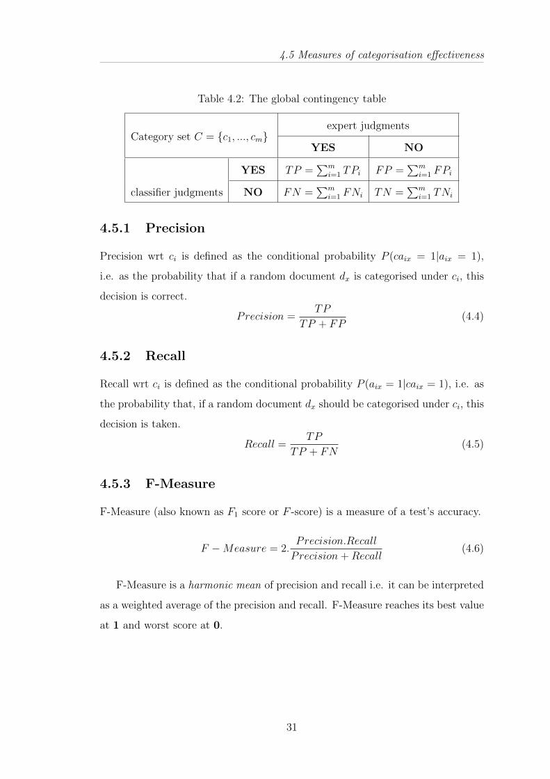
Table 4.2: The global contingency table
Category set C = {c1, ..., cm}expert judgments
YES NO
classifier judgments
YES TP =∑m
i=1 TPi FP =∑m
i=1 FPi
NO FN =∑m
i=1 FNi TN =∑m
i=1 TNi
4.5.1 Precision
Precision wrt ci is defined as the conditional probability P (caix = 1|aix = 1),
i.e. as the probability that if a random document dx is categorised under ci, this
decision is correct.
Precision =TP
TP + FP(4.4)
4.5.2 Recall
Recall wrt ci is defined as the conditional probability P (aix = 1|caix = 1), i.e. as
the probability that, if a random document dx should be categorised under ci, this
decision is taken.
Recall =TP
TP + FN(4.5)
4.5.3 F-Measure
F-Measure (also known as F1 score or F -score) is a measure of a test’s accuracy.
F −Measure = 2.P recision.Recall
Precision+Recall(4.6)
F-Measure is a harmonic mean of precision and recall i.e. it can be interpreted
as a weighted average of the precision and recall. F-Measure reaches its best value
at 1 and worst score at 0.
31

4.6 Performance Analysis
4.6 Performance Analysis
The figures 4.1, 4.2 and 4.3 shows the performance comparison for the selected
benchmarking algorithms of WEKA with three different percentage split of the
training set and three feature selection techniques namely term frequency (TF),
information gain (IG) and chi-square (χ2) for the NFS Abstract-Title dataset.
Figure 4.1: Performance for different classifiers using Information Gain for NFSAbstract-Title dataset
With information gain, Nave Bayes Multinomial performance listed low com-
pared to other classifiers for both traditional (without annotation) as well as our
approach (with annotation). Here ‘without annotation’ denotes without and ‘with
annotation’ denotes with in the figures. The highest performance is recorded for
SMO and J48 i.e. from 0.45 to 0.74 with 70% split for SMO training set and from
0.46 to 0.787 with 50% split for J48. Figure 4.1 shows the performance compari-
son for different classifiers with annotation and without annotation for information
gain as a feature selection methodology.
With chi-square (χ2), performance gain noticed was highest for J48 and Nave
Bayes Multinomial with 50% split. With annotation an average performance ac-
32

4.6 Performance Analysis
Figure 4.2: Performance for different classifiers using Term Frequency for NFSAbstract-Title dataset
Figure 4.3: Performance for different classifiers using Chi-Square for NFSAbstract-Title dataset
curacy observed was highest with chi-square feature selection methodology.
With term frequency, we observed that Nave Bayes Multinomials performance
was good for both the approaches than the performance for information gain.
SMO gave highest accuracy i.e. from 0.563 for without annotation and 70% split
to 0.73 with annotation. An average performance for 70% split for training dataset
is higher than 50% and 30% split. In Figure 4, we have shown F-Measure of
33

4.6 Performance Analysis
different classifiers for both the approaches with term frequency.
Figure 4.4: Performance for different classifiers using term frequency for Reuters-21578
Figure 4.4 shows the results obtained for Reuters-21578 with annotation and
without annotation technique. Our technique of feature annotation gave little less
performance for Reuters-21578 dataset. This is because the dataset contains a lot
less dimensions that we have extracted for annotation. And, for NFS Abstract
dataset, it has all the dimensions that we have considered for annotation, so
observed performance was better for NFS Abstract dataset.
In case of Reuters-21578, with 50% split and for SMO there is a little improve-
ment in accuracy. But, for NFS-Abstract dataset we observed improved classifica-
tion accuracy for three percentage splits that we have considered and for all three
feature selection methods i.e. term-frequency, information gain and chi-square.
Overall performance of all the classifiers with term-frequency was good for both
without annotation and with annotation as compared to information gain and
chi-square.
Table 4.3 shows the F-Measure for real time Cricket dataset for both the ap-
proaches i.e. without annotation and with annotation and with term frequency as
34

4.6 Performance Analysis
Table 4.3: F-Measure for real time Cricket dataset
``````````````̀ApproachClassifier
NBM SMO J48 JRip Bagging
Without Annotation 0.912 0.898 0.815 0.784 0.831
With Annotation 0.913 0.918 0.859 0.859 0.866
Table 4.4: F-Measure for Reuters-21578 dataset
``````````````̀ApproachClassifier
NBM SMO J48 JRip Bagging
Without Annotation 0.696 0.608 0.590 0.563 0.548
With Annotation 0.712 0.587 0.539 0.554 0.552
a feature selection approach. It can be observed that there is marginal performance
improvement in classification using annotated features for Cricket dataset.
For the Cricket dataset overall performance observed for NBM was good com-
pared to other classifiers. After annotation JRip gave better improvement in
accuracy i.e. from 0.784 to 0.859.
Reuters-21578 dataset doesnt contain entities which we extracted for annotation
in much quantity. So, we observed that there is not significant result improvement.
Table 4.4 shows the F-measure for different classifiers with information gain feature
selection method.
Table 4.5 represents the collective result for NFS Abstract dataset. In this table
results for different feature selection methods along with both the approaches i.e.
with- with annotation and w/o- without annotation and for three percentage splits
for training data and test data, such as 70%, 50% and 30% is shown, also, for five
different classifiers mentioned above.
35

4.6 Performance Analysis
Table 4.5: F-Measure for NFS Abstract dataset
PPPPPPPPPPPClassifiers
FS Term Frequency Information Gain Chi-Square
W/O With W/O With W/O With
NBM
70% 0.467 0.510 0.322 0.389 0.486 0.738
50% 0.476 0.516 0.302 0.242 0.538 0.784
30% 0.468 0.487 0.226 0.229 0.526 0.703
SMO
70% 0.563 0.730 0.450 0.740 0.450 0.740
50% 0.553 0.677 0.468 0.726 0.468 0.726
30% 0.535 0.618 0.465 0.672 0.465 0.672
J48
70% 0.409 0.610 0.520 0.758 0.513 0.758
50% 0.558 0.591 0.460 0.787 0.460 0.787
30% 0.450 0.527 0.476 0.656 0.475 0.656
JRip
70% 0.452 0.570 0.398 0.617 0.396 0.661
50% 0.495 0.586 0.370 0.687 0.430 0.652
30% 0.409 0.464 0.351 0.461 0.351 0.461
Bagging
70% 0.611 0.608 0.549 0.716 0.549 0.716
50% 0.523 0.599 0.536 0.684 0.536 0.673
30% 0.453 0.513 0.452 0.640 0.452 0.640
36

4.7 Results of Recommendation Engine
4.7 Results of Recommendation Engine
As there are no standard systems available to compare the results of our recom-
mendation engine, so to represent the results of this module we have considered
some examples and have shown how the system works.
Example Profiles:
User Profile=1
Name: Santosh Kalamkar
Edu. Qualification: Post Graduate
Interest area Rating Keywords
1. Natural Language Processing 3 <context, annotation>
2. Networking 2 <packet routing>
3. Network Security 3 <encryption algorithms>
User Profile=2
Name: S. Kalamkar
Edu. Qualification: Under Graduate
Interest areas Rating Keywords
1. Natural Language Processing 4 <classifiers, SVM>
2. HPC 4 <GPGPU, CUDA>
3. Network Security 5 <encryption algorithms>
Paper Profiles:
Paper ID Title Rating Keywords Domain
37

4.7 Results of Recommendation Engine
P1 Feature Extraction for TC 4.00 <text, feature> NLP
P2 PIR Cache Implementation 2.00 <PIR, cache, security> NS
P3 Network building in MT 5.00 <MT, network> NW
As mentioned before, for every recommendation we are taking two inputs from
user: 1. Paper Rating and 2. Level Rating. We calculate average rating for
every paper belonging to the same domain as that of the user interest. And,
considering users rating for his interest area and papers average rating, if the
paper satisfies rules as mentioned in Table 3.2, we put that paper in the list of
the papers for recommendations. In case of level rating, again we calculate the
average rating and if the paper satisfies rules as in Table 3.3, we add this paper to
the recommendation list. If the paper has keywords as entered by user (and both
has same domain), we are adding this paper too in recommendation list. And,
out of the list of the recommendation papers we recommend only five randomly
selected results to user.
For user profile 1, rate of domain ‘Natural Language Processing’ is 3, and for
paper ‘P1’ average rating is 4.00, it satisfies rule as in Table 3.2, we add this paper
in recommendation list. But paper ‘P2’ does not satisfy the rule of this table so we
are not considering this paper for recommendation. In case of paper P3 average
rating is 3.00, so it will be in the list of recommendations to user 1. In the same
way we find the recommendations to user 2.
Finally, the recommendation lists of each user are as follows:
User 1:
1. Feature Extraction for TC
2. Network building in MT
User 2:
1. Feature Extraction for TC
38

4.7 Results of Recommendation Engine
2. PIR Cache Implementation
Here, for User 1 and User 2 one common paper is recommended i.e. ‘Feature
Extraction for TC’, this is because of having same interest domain of both the
users and this paper satisfies the recommendation rules explained above. For User
1 second recommendation is from domain ‘Networking’, and for User 2 second
recommendation is from domain ‘Network Security’. Even though they have same
interest domain ‘Network Security’, User 1’s rating is less compared to User 2.
Therefore this paper is recommended to only User 2.
39

Chapter 5
Conclusion and Future Work
In this chapter we enlist the conclusion drawn from the project work and the
future work that can be carried out.
5.1 Conclusion
From performance analysis, we can conclude that the four dimensions i.e. spatial,
temporal, protagonist and organization actually contribute in improving the accu-
racy of the classification. The NFS Abstract dataset and real time cricket dataset
we selected contains different dimensions of our interest i.e. person names, lo-
cation information, temporal information and organization in high quantity as
compared to Reuters-21578 dataset. These contextual features acts as a major
contributors in the text classification process. So, the accuracy of classification
for NFS Abstract dataset and cricket dataset is high compared to Reuters-21578.
Once the data is classified, we may use it effectively for further purpose. As we
have shown with recommendation engine, we can recommend the research papers
to the user based on his/her educational qualification, interest area and other
contextual information. This type of systems can be used in applications where
the available dataset size is very huge, and it’s not possible for a user to go through
every classified instance.
40
5.2 Future Work
5.2 Future Work
By considering more dimensions i.e. context as well as considering co-references we
can make improvement in the text classification. We can also use these dimensions
to build human mental situation model for classification. Also using the available
context we can exploit context-topic relationship by designing contextual topic
model and considering all possible dependency structures of context. By applying
contextual text mining in the context of other text information management tasks,
including ad hoc text retrieval and web search, we may prove the effectiveness of
contextual text mining techniques in a quantitative way.
41

Appendix A
Publications
This section is related to the research papers that have been published.
A.1 Feature Annotation for Text Categorization
Authors: Santosh Kalamkar, Yashodhara Haribhakta, Dr. Parag Kulkarni
Conference: CUBE 2012 International IT conference and Exhibition
Publisher: ACM ICPS (International Conference Proceedings Series )
Conference URL: http://www.thecubeconf.com/
Status: Accepted and submitted for publication
42

Bibliography
[1] Zi-jun Yu; Wei-gang Wu; Jing Xiao; Jun Zhang; Rui-Zhang
Huang; Ou Liu. 2009. Keyword Combination Extraction in
Text Categorization Based on Ant Colony Optimization. Soft
Computing and Pattern Recognition, 2009. SOCPAR ’09. Inter-
national Conference of, vol., no., pp.430-435, 4-7 Dec. 2009. DOI:
10.1109/SoCPaR.2009.90
http://ieeexplore.ieee.org/stamp/stamp.jsp?tp=
&arnumber=5368629&isnumber=5368599..
[2] Fabrizio Sebastiani. 2002. Machine learning in automated text
categorization. ACM Comput. Surv. 34, 1 (March 2002), 1-47.
DOI=10.1145/505282.505283
http://doi.acm.org/10.1145/505282.505283
[3] Chua, S., Kulathuramaiyer, N. 2004. Semantic Feature Selection
Using WordNet. Web Intelligence, 2004. WI 2004. Proceedings.
IEEE/WIC/ACM International Conference on, vol., no., pp. 166-
172, 20-24 Sept. 2004 DOI: 10.1109/WI.2004.10115
http://ieeexplore.ieee.org/stamp/stamp.jsp?tp=
&arnumber=1410799&isnumber=30573
[4] Sayali Kulkarni, Amit Singh, Ganesh Ramakrishnan, and Soumen
Chakrabarti. 2009. Collective annotation of Wikipedia enti-
ties in web text. In Proceedings of the 15th ACM SIGKDD
international conference on Knowledge discovery and data
mining (KDD ’09). ACM, New York, NY, USA, 457-466.
DOI=10.1145/1557019.1557073
http://doi.acm.org/10.1145/1557019.1557073
[5] Yi Guo, Zhiqing Shao, Nan Hua.2010. Automatic text categoriza-
tion based on content analysis with cognitive situation models.
43
BIBLIOGRAPHY
Information Sciences, Volume 180, Issue 5, 1 March 2010, Pages
613-630, ISSN 0020-0255, 10.1016/j.ins.2009.11.012
http://www.sciencedirect.com/science/article/pii/
S00200255609004824
[6] Bontcheva, K., Cunningham, H., Maynard, D., Tablan, V.
and Saggion, H. 2002. Developing reusable and robust language
processing components for information systems using GATE.
Database and Expert Systems Applications, 2002. Proceedings.
13th International Workshop on , vol., no., pp. 223- 227, 2-6 Sept.
2002 DOI: 10.1109/DEXA.2002.1045902
http://ieeexplore.ieee.org/stamp/stamp.jsp?tp=
&arnumber=1045902&isnumber=22410
[7] Keno Buss. 2007. Literature Review on Preprocessing for Text
Mining.
http://dmuca.ioct.dmu.ac.uk/publication/papers/
literature_review_keno.pdf
[8] Monica Rogati and Yiming Yang. 2002. High-performing feature
selection for text classification. In Proceedings of the eleventh
international conference on Information and knowledge man-
agement (CIKM ’02). ACM, New York, NY, USA, 659-661.
DOI=10.1145/584792.584911
http://doi.acm.org/10.1145/584792.584911
[9] Isabelle Guyon and Andr Elisseeff. 2003. An introduction to variable
and feature selection. J. Mach. Learn. Res. 3 (March 2003), 1157-
1182.
[10] Ron Kohavi and George H. John. 1997. Wrappers for feature
subset selection. Artif. Intell. 97, 1-2 (December 1997), 273-324.
DOI=10.1016/S0004-3702(97)00043-X
http://dx.doi.org/10.1016/S0004-3702(97)00043-X
[11] M. F. Zaiyadi and Baharudin. 2010. A proposed hybrid approach for
feature selection in text document categorization. World academy of
science, engineering and technology 72-2010.
44

BIBLIOGRAPHY
[12] A. Frank and A. Asuncion. UCI Machine Learning Repository,
2010.
http://archive.ics.uci.edu/ml
[13] E. Frank, M. Hall, G. Holmes, R. Kirkby, B. Pfahringer, I. Wit-
ten, and L. Trigg. Weka. Data Mining and Knowledge Discovery
Handbook, pages 1305-1314, 2005.
[14] Wang Xiaoyue and Bai Rujiang. Applying RDF Ontologies to Im-
prove Text Classification. Computational Intelligence and Natural
Computing, 2009. CINC ’09. International Conference on , vol.2,
no., pp.118-121, 6-7 June 2009 doi: 10.1109/CINC.2009.115.
http://ieeexplore.ieee.org/stamp/stamp.jsp?tp=
&arnumber=5231026&isnumber=5230911
[15] Lewis, D. Reuters-21578. 1997[Online]. Available:
http://www.daviddlewis.com/resources/testcollections/
reuters21578/
[16] World Wide Web Size
http://www.worldwidewebsize.com/
[17] Fellbaum C. 1998. Wordnet: An electronic lexical database. Cam-
bridge: MIT Press.
[18] Wikipedia
http://en.wikipedia.org/wiki/Unstructureddata
[19] Francois Paradis, Jian-Yun Nie. 2007. Contextual feature selection
for text classification. Special issue on AIRS2005: Information
Retrieval Research in Asia. 1016/j.ipm.2006.07.006.
http://www.sciencedirect.com/science/article/pii/
S0306457306001269
[20] Tan, Chade-Meng and Wang, Yuan-Fang and Lee, Chan-Do. 2002.
The use of bigrams to enhance text categorization. Inf. Process.
Manage. 10.1016/S0306-4573(01)00045-0.
http://dx.doi.org/10.1016/S0306-4573(01)00045-0
[21] Pang, B., Lee L., Vaithyanathan , S. (2002). Thumbs up? Sentiment
Classification Using Machine Learning Techniques. EMNLP.
45

BIBLIOGRAPHY
[22] Yu, Hong and Hatzivassiloglou, Vasileios. 2003. Towards answering
opinion questions: separating facts from opinions and identifying
the polarity of opinion sentences. Proceedings of the 2003 confer-
ence on Empirical methods in natural language processing, ACL.
10.3115/1119355.1119372.
http://dx.doi.org/10.3115/1119355.1119372
[23] Jansche, Martin. 2002. Named entity extraction with conditional
Markov models and classifiers. proceedings of the 6th confer-
ence on Natural language learning - Volume 20, COLING-02.
10.3115/1118853.1118866.
http://dx.doi.org/10.3115/1118853.1118866
[24] Fragoudis, Dimitris and Meretakis, Dimitris and Likothanassis,
Spiros. 2002. Integrating feature and instance selection for text clas-
sification. Proceedings of the eighth ACM SIGKDD international
conference on Knowledge discovery and data mining, KDD ’02.
10.1145/775047.775120.
http://doi.acm.org/10.1145/775047.775120
[25] George H. John and Ron Kohavi and Karl Pfleger. 1994. Irrelevant
Features and the Subset Selection Problem. MACHINE LEARN-
ING: PROCEEDINGS OF THE ELEVENTH INTERNATIONAL,
121-129.
[26] J. Firth. Ethnographic analysis and language with reference to ma-
linowskis views. Man and Culture: An Evaluation of the Work of
Bronislaw Malinowski., 1957.
[27] J. R. Firth. A synopsis of linguistic theory, 1930-1955. Studies in
Linguistic Analysis, pages 1-32,1957.
[28] D. Gruhl, R. Guha, R. Kumar, J. Novak, and A. Tomkins. The pre-
dictive power of online chatter. In Proceedings of KDD ’05, pages
78-87, 2005.
[29] J. Kleinb erg. Bursty and hierarchical structure in streams. In
Proceedings of KDD ’02, pages 91-101, 2002
46

BIBLIOGRAPHY
[30] Q. Mei and K. Church. Entropy from search logs: How hard is
search? with personalization? with backoff?. In Proceeding of
WSDM’08, pages 45-54, 2008.
[31] Q. Mei, X. Ling, M. Wondra, H. Su, and C. Zhai. Topic sentiment
mixture: Modeling facets and opinions in weblogs. In Proceedings
of WWW ’07, 2007.
[32] M. Steyvers, P. Smyth, M. Rosen-Zvi, and T. Griffiths. Probabilistic
author-topic models for information discovery. In Proceedings of
KDD ’04, pages 306-315, 2004.
[33] T. van Dijk. Text and context. Longman , 1977.
[34] International Cricket Council- ICC Events, ICC Cricket Rankings,
Live Cricket Scores, ODI Fantasy League, Test Predictor
http://icc-cricket.yahoo.net/
[35] Hui Wang, Sally McClean. 2003. Classification based on contextual
probability. 2003.
[36] Marco Ernandes et a. 2007. An Adaptive Context Based Algorithm
for Term Weighting. Proceedings of the 20th international joint
conference on Artifical intelligence, 2748- 2753, 2007
[37] Qiaozhu Mei and ChengXiang Zhai. 2006. A mixture model
for contextual text mining. In Proceedings of the 12th ACM
SIGKDD international conference on Knowledge discovery and
data mining (KDD ’06). ACM, New York, NY, USA, 649-655.
DOI=10.1145/1150402.1150482
http://doi.acm.org/10.1145/1150402.1150482
[38] T. Hofmann. 1999. Probabilistic latent semantic analysis. In Pro-
ceedings of ’99.
[39] T. Hofmann. 1999. The cluster-abstraction model: Unsupervised
learning of topic hierarchies from text data. In IJCAI’ 99, pages
682-687, 1999.
[40] Z. Li, B. Wang, M. Li, and W.-Y. Ma. A probabilistic model for
retrospective news event detection. In Proceedings of SIGIR ’05,
pages 106-113, 2005.
47