Embed Size (px)
Citation preview

i
IntelliHealth: An intelligent medical decision support system using a novel
multi-layer classifier ensemble framework based on enhanced bagging
approach with multi-objective optimized weighted voting scheme
Author
Saba Bashir
2010-NUST-TfrPhD-CSE-59
Supervisor
Dr. Usman Qamar
Department of Computer Engineering
College of Electrical & Mechanical Engineering
National University of Sciences & Technology
Islamabad
2016

ii
IntelliHealth: An intelligent medical decision support system using a novel
multi-layer classifier ensemble framework based on enhanced bagging
approach with multi-objective optimized weighted voting scheme
Author
SABA BASHIR
Regn Number: 2010-NUST-TfrPhD-CSE-59
A thesis submitted in partial fulfillment of the requirements for the degree of
DOCTOR OF PHILOSOPHY
in
COMPUTER SOFTWARE ENGINEERING
Thesis Supervisor
DR. USMAN QAMAR
Signature:______________________________
Department of Computer Engineering
College of Electrical & Mechanical Engineering
National University of Sciences & Technology
Islamabad
2016

iii
Declaration
I certified that this research work titled ―IntelliHealth: An intelligent medical
decision support system using a novel multi-layer classifier ensemble
framework based on enhanced bagging approach with multi-objective optimized
weighted voting scheme‖ is my own work. The work has not been presented
elsewhere for assessment. The material that has been used from other sources it
has been properly acknowledged /referred.
Signature: _________________
Saba Bashir
2010-NUST-TfrPhD-CSE-59

iv
Acknowledgements
First of all, I would like to thank Allah Almighty who gave me the ability and
bestowed me with perseverance to complete this thesis. He is the ONE I always
looked to in the event of trouble and He always created a way for me out of the
trouble. I would not be what I am today If He did not want me to be.
I would like to express my deep-felt gratitude to my advisor, Dr. Usman Qamar,
Assistant Professor in Computer Engineering Department, for his advice,
encouragement, enduring patience and constant support. He was never ceasing
his belief in me, always providing clear explanations when I was lost and
always giving me his time, in spite of anything else that was going on.
I gratefully acknowledge my committee members, Dr. M. Younus Javed, Dean
HITEC University, Dr. Saad Rehman, College of E&ME and Dr. Rehan Hafiz
from ITU, Lahore.
Last but not the least, I would like to appreciate and thanks my parents, family
and specially my husband for his continuous motivation, support and help
throughout my thesis work.
v
Abstract
Decision support is a crucial function for decision makers in many industries. Typically,
decision support systems (DSS) help decision-makers to gather and interpret information and
build a foundation for decision-making. Medical Decision Support Systems (MDSS) play an
increasingly important role in medical practice. By assisting doctors with making clinical
decisions, DSS are expected to improve the quality of medical care. Conventional clinical
decision support systems are based on individual classifiers or simple combination of these
classifiers which tend to show moderate performance. In this thesis, we presented a novel
multi-layer classifier ensemble framework based on enhanced bagging approach with multi-
objective optimized weighted voting scheme for prediction of multiple diseases. The
proposed model named ―HM-BagMoov‖ (Hierarchical Multi-level classifiers Bagging with
Multi-objective Weighted voting) overcomes the limitations of conventional performance
bottlenecks by utilizing an ensemble of seven heterogeneous classifiers: Naïve Bayes, Linear
Regression, Linear Discriminant Analysis, K Nearest Neighbor, Support Vector Machine,
Artificial Neural Network ensemble and Random Forest. The proposed ensemble framework
utilizes different preprocessing techniques such as missing value imputation, feature
selection, outlier detection and noise removal to improve the quality of data. Five different
heart disease datasets, four breast cancer datasets, two diabetes datasets, two liver datasets
and one hepatitis dataset are used for experimentation, evaluation and validation. The datasets
are obtained from publicly available data repositories. Effectiveness of the proposed
ensemble is investigated by comparison of results with several well-known classifiers as well
as with ensembles. The experimental evaluation shows that the proposed framework dealt
with all type of attributes and achieved high diagnosis accuracy. The f-ratio higher than f-
critical and p-value less than 0.05 for 95% confidence interval indicate that the results are
statistically significant for most of the datasets. Using HM-BagMoov we have developed an
application called ―IntelliHealth‖ that may be used by hospitals/doctors for diagnostic advice.
vi
Table of Contents
Declaration.................................................................................................................................... iii
Acknowledgements ...................................................................................................................... iv
Abstract .......................................................................................................................................... v
Table of Contents ......................................................................................................................... vi
Chapter 1: 1ntroduction ............................................................................................................... 1
1.1 Data Mining and Machine Learning ...................................................................................... 5
1.2 Motivation ............................................................................................................................. 6
1.3 Challenges in Health Sector .................................................................................................. 6
1.3.1 Large Volume of Medical Data ...................................................................................... 6
1.3.2 Data Quality .................................................................................................................... 6
1.3.3 Data Privacy and Ethical issue ....................................................................................... 7
1.3.4 Expensive Implementation of Data Warehousing .......................................................... 7
1.4 Clinical Decision Support Framework .................................................................................. 7
1.5 Research Problems ................................................................................................................ 8
1.6 Contributions ......................................................................................................................... 9
1.7 ―IntelliHealth‖ Application for Disease Diagnosis ............................................................. 11
1.8 Organization of the thesis .................................................................................................... 12
1.9 Summary ............................................................................................................................. 12
Chapter 2: Background .............................................................................................................. 13
2.1 Machine Learning Methods ................................................................................................ 13
2.1.1 Naïve Bayes (NB) ......................................................................................................... 14
2.1.2 Decision Tree Induction based on Gini Index (DT-GI) ............................................... 14
2.1.3 Decision Tree Induction based on Information Gain (DT-IG) ..................................... 16
2.1.4 Decision Tree Induction based on Gain Ratio (DT-GR) .............................................. 16
2.1.5 Memory based Learner (MBL) ..................................................................................... 17
2.1.6 Support Vector Machine (SVM) .................................................................................. 19
2.1.7 Linear Regression (LR) ................................................................................................ 20
2.1.8 Linear Discriminant Analysis (LDA) ........................................................................... 21
2.1.9 Artificial Neural Network (ANN) .............................................................................. 223
2.2 Ensemble Techniques .......................................................................................................... 24
2.2.1 Random Forest (RF) ..................................................................................................... 24
vii
2.2.2 Majority Voting Ensemble ........................................................................................... 25
2.2.3 Bagging Ensemble ........................................................................................................ 27
2.2.4 AdaBoost Ensemble ..................................................................................................... 27
2.2.5 Stacking Ensemble ....................................................................................................... 29
2.3 Clinical Decision Support Systems ..................................................................................... 29
2.4 Summary ............................................................................................................................. 32
Chapter 3: State of the Art Techniques in Medical Domain .................................................. 33
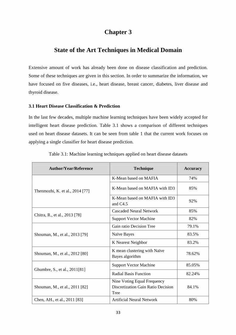
3.1 Heart Disease Classification & Prediction ...................................................................... 33
3.2 Breast Cancer Classification & Prediction .................................................................... 334
3.3 Diabetes Classification & Prediction ............................................................................... 36
3.4 Liver Disease Classification & Prediction ....................................................................... 38
3.5 Hepatitis Classification & Prediction .............................................................................. 39
3.6 Summary ............................................................................................................................. 40
Chapter 4: Research Methodology ............................................................................................ 41
4.1 Utilization of Ensemble frameworks................................................................................... 41
4.2 Homogeneous Ensemble Frameworks ................................................................................ 41
4.3 Heterogeneous Ensemble Frameworks ............................................................................... 44
4.3.1 Majority Voting Ensemble Scheme .............................................................................. 44
4.3.2 Weighted Voting Ensemble Scheme ............................................................................ 47
4.4 Hierarchical Multi-level classifiers Bagging with Multi-objective optimized voting
(HM-BagMoov) Framework ..................................................................................................... 56
4.5 Summary ............................................................................................................................. 65
Chapter 5: Experimental Results .............................................................................................. 66
5.1 Datasets ............................................................................................................................... 66
5.1.1 Heart Disease Datasets ................................................................................................. 66
5.1.2 Breast Cancer Datasets ................................................................................................. 69
5.1.3 Diabetes Datasets .......................................................................................................... 73
5.1.4 Liver Disease Datasets .................................................................................................. 74
5.1.5 Hepatitis Disease Dataset ............................................................................................. 76
5.2 Results and Discussion ........................................................................................................ 77
5.2.1 Evaluation Metrics ........................................................................................................ 77
5.2.2 Multi-Disease Prediction .............................................................................................. 78
5.2.2.1 Heart Disease Classification and Prediction ...................................................... 78
5.2.2.2 Breast Cancer Classification and Prediction ...................................................... 81
viii
5.2.2.3 Diabetes Classification and Prediction .............................................................. 83
5.2.2.4 Liver Disease Classification and Prediction ...................................................... 85
5.2.2.5 Hepatitis Classification and Prediction .............................................................. 87
5.2.3 Discussion ..................................................................................................................... 88
5.2.4 ANOVA Statistics ........................................................................................................ 89
5.2.4.1 Heart Disease Datasets ....................................................................................... 90
5.2.4.2 Breast Cancer Datasets ...................................................................................... 93
5.2.4.3 Diabetes Datasets ............................................................................................... 94
5.2.4.4 Liver Disease Datasets ....................................................................................... 95
5.2.4.5 Hepatitis Dataset ................................................................................................ 96
5.3 Analysis of HM-BagMoov .................................................................................................. 96
5.4 Summary ............................................................................................................................. 99
Chapter 6: IntelliHealth: An Intelligent Application for Disease Diagnosis ....................... 100
6.1 IntelliHealth Medical Application ..................................................................................... 100
6.1.1 Modules of IntelliHealth ............................................................................................. 100
6.1.2 Users of Proposed IntelliHealth Application .............................................................. 103
6.2 Case Studies ...................................................................................................................... 106
6.3 Summary ........................................................................................................................... 106
Chapter 7: Conclusion and Future Work ............................................................................... 112
7.1 Conclusion ....................................................................................................................... 1122
7.2 Future Work ....................................................................................................................... 113
7.3 Final Word......................................................................................................................... 112
References .................................................................................................................................. 115
Publications ............................................................................................................................... 126
ix
List of Figures
Figure 1.1: Data mining process in healthcare ............................................................................... 1
Figure 1.2: Structure of heart and ECG of a person with heart disease ......................................... 2
Figure 1.3: Symptoms of Breast cancer disease in females ........................................................... 2
Figure 1.4: Insufficient production of insulin causes diabetes ...................................................... 3
Figure 1.5: Various stages of liver damage during liver disease ................................................... 4
Figure 1.6: Structure of hepatitis A,B,C,D and E virus ................................................................. 4
Figure 1.7: Generic data mining ensemble framework for disease prediction and evaluation ....... 7
Figure 1.8: DSS for real-time clinical practice ............................................................................... 9
Figure 1.9: Generic illustration of proposed ensemble framework .............................................. 10
Figure 1.10: Proposed Intellihealth Application ........................................................................... 11
Figure 2.1: General approach for building a classification model ................................................ 13
Figure 2.2: Decision tree representing multiple splitting attributes .............................................. 15
Figure 2.3: K nearest neighbors of an instance x .......................................................................... 18
Figure 2.4: Examples of SVM classifier to classify data into two classes ................................... 19
Figure 2.5: Linear regression model ............................................................................................. 21
Figure 2.6: Data with fixed and quadratic covariance .................................................................. 22
Figure 2.7: Basic structure of an Artificial Neural Network ........................................................ 23
Figure 2.8: Ensemble classifier by combining several individual classifiers ............................... 24
Figure 2.9: Random forest classification tree ............................................................................... 25
Figure 2.10: Majority voting ensemble framework ...................................................................... 26
Figure 2.11: Hypothetical runs of Bagging................................................................................... 27
Figure 2.12: Boosting ensemble classifier framework ................................................................. 28
Figure 2.13: Stacking ensemble classifier framework .................................................................. 29
Figure 2.14: Fuzzy based clinical decision support framework for heart disease prediction ....... 30
Figure 2.15: Proposed clinical decision support framework for breast cancer prediction ............ 31
Figure 2.16: Proposed clinical decision support framework for diabetes prediction ................... 32
Figure 4.1: Majority Voting based homogeneous Ensemble Framework .................................... 42
Figure 4.2: Boosting based homogeneous Ensemble Framework ................................................ 42
Figure 4.3: Stacking based homogeneous ensemble framework .................................................. 43
Figure 4.4: Bagging based homogeneous ensemble framework .................................................. 44
Figure 4.5: Schematic illustration of MV3 ensemble framework................................................. 45
Figure 4.6: Detailed architecture of proposed MV5 ensemble framework .................................. 47
x
Figure 4.7: AccWeight Ensemble Framework for Disease Diagnosis ......................................... 49
Figure 4.8: Flowchart of FmWeight ensemble model .................................................................. 52
Figure 4.9: BagMOOV ensemble algorithm ................................................................................. 54
Figure 4.10: Flow diagram of preprocessing ................................................................................ 58
Figure 4.11: Proposed missing data imputation method ............................................................... 61
Figure 4.12: Flow diagram of classifier training module ............................................................. 63
Figure 4.13: Detailed architecture of proposed ensemble framework .......................................... 64
Figure 6.1: Architecture of proposed IntelliHealth application ................................................. 100
Figure 6.2: Add patient‘s detail screen ....................................................................................... 101
Figure 6.3: Load training set and generate model screen ........................................................... 102
Figure 6.4: Diagnose patient screen displayed to doctor ............................................................ 103
Figure 6.5: Start screen of proposed application ........................................................................ 104
Figure 6.6: Login screen of proposed application ...................................................................... 104
Figure 6.7: Dashboard screen of proposed IntelliHealth application ........................................ 105
Figure 6.8: Implementing IntelliHealth in real-time clinical practice ....................................... 106
xi
List of Tables
Table 1.1: Three stages of knowledge discovery in databases (KDD) ........................................... 5
Table 3.1: Data mining techniques applied on heart disease datasets ......................................... 33
Table 3.2: Data mining techniques applied on breast cancer datasets ......................................... 34
Table 3.3: Data mining techniques applied on diabetes datasets ................................................. 36
Table 3.4: Data mining techniques applied on liver disease datasets .......................................... 38
Table 3.5: Data mining techniques applied on hepatitis disease datasets .................................... 39
Table 5.1: SPECT dataset sample ................................................................................................ 66
Table 5.2: SPECTF dataset sample .............................................................................................. 67
Table 5.3: Statlog dataset sample ................................................................................................. 68
Table 5.4: A sample of heart disease dataset ............................................................................... 69
Table 5.5: Eric dataset sample ...................................................................................................... 69
Table 5.6: BCD dataset sample ..................................................................................................... 70
Table 5.7: WDBC dataset sample ................................................................................................. 70
Table 5.8: WBC dataset sample .................................................................................................... 71
Table 5.9: WPBC dataset sample.................................................................................................. 72
Table 5.10: PIDD dataset sample .................................................................................................. 73
Table 5.11: Biostat diabetes dataset sample ................................................................................. 74
Table 5.12: Bupa liver disease dataset sample.............................................................................. 75
Table 5.13: ILPD liver disease dataset sample ............................................................................. 76
Table 5.14: Hepatitis dataset sample ............................................................................................ 76
Table 5.15: Traditional Confusion Matrix .................................................................................... 78
Table 5.16: Comparison of HM-BagMoov with individual classifiers ........................................ 78
Table 5.17: Comparison of HM-BagMoov with ensembles ......................................................... 79
Table 5.18: Statistical Comparison of HM-BagMoov with State of the Art Techniques ............. 80
Table 5.19: Comparison of HM-BagMoov with individual classifiers ........................................ 81
Table 5.20: Comparison of HM-BagMoov with ensembles ......................................................... 82
Table 5.21: Comparison of HM-BagMoov with State of the Art Techniques ............................ 82
Table 5.22: Comparison of HM-BagMoov with individual classifiers ........................................ 83
Table 5.23: Comparison of HM-BagMoov with ensembles ......................................................... 84
Table 5.24: Comparison of HM-BagMoov with State of the Art Techniques ............................ 84
Table 5.25: Comparison of HM-BagMoov with individual classifiers ........................................ 85
Table 5.26: Comparison of HM-BagMoov with ensembles ......................................................... 85
xii
Table 5.27: Comparison of HM-BagMoov with State of the Art Techniques ............................ 86
Table 5.28: Comparison of HM-BagMoov with individual classifiers ........................................ 87
Table 5.29: Comparison of HM-BagMoov with ensembles ......................................................... 87
Table 5.30: Comparison of HM-BagMoov with State of the Art Techniques .............................. 88
Table 5.31: ANOVA Statistics for Cleveland heart disease dataset ............................................. 91
Table 5.32: ANOVA Statistics for SPECT dataset ....................................................................... 91
Table 5.33: ANOVA Statistics for Statlog dataset ....................................................................... 91
Table 5.34: ANOVA Statistics for SPECTF dataset .................................................................... 92
Table 5.35: ANOVA Statistics for Eric dataset ............................................................................ 92
Table 5.36: ANOVA Statistics for UMC breast cancer dataset.................................................... 93
Table 5.37: ANOVA Statistics for WDBC dataset ....................................................................... 93
Table 5.38: ANOVA Statistics for WPBC dataset ....................................................................... 94
Table 5.39: ANOVA Statistics for WBC dataset.......................................................................... 94
Table 5.40: ANOVA Statistics for Biostat diabetes dataset ......................................................... 94
Table 5.41: ANOVA Statistics for PIDD dataset ......................................................................... 95
Table 5.42: ANOVA Statistics for ILPD dataset .......................................................................... 95
Table 5.43: ANOVA Statistics for BUPA liver dataset ................................................................ 96
Table 5.44: ANOVA Statistics for hepatitis dataset ..................................................................... 96
Table 5.45: Average accuracy of single classifiers for multiple diseases ..................................... 97
Table 5.46: Average accuracy of ensemble classifiers for multiple diseases ............................... 97
Table 6.1: RIC dataset features for heart disease ........................................................................ 108
Table 6.2: PIMS CP dataset features for disease prediction ....................................................... 109
Table 6.3: An example of if-then rules generated by proposed DSS .......................................... 110
Table 6.4: Diagnosis comparison for individual patients ........................................................... 110
1
Chapter 1
Introduction
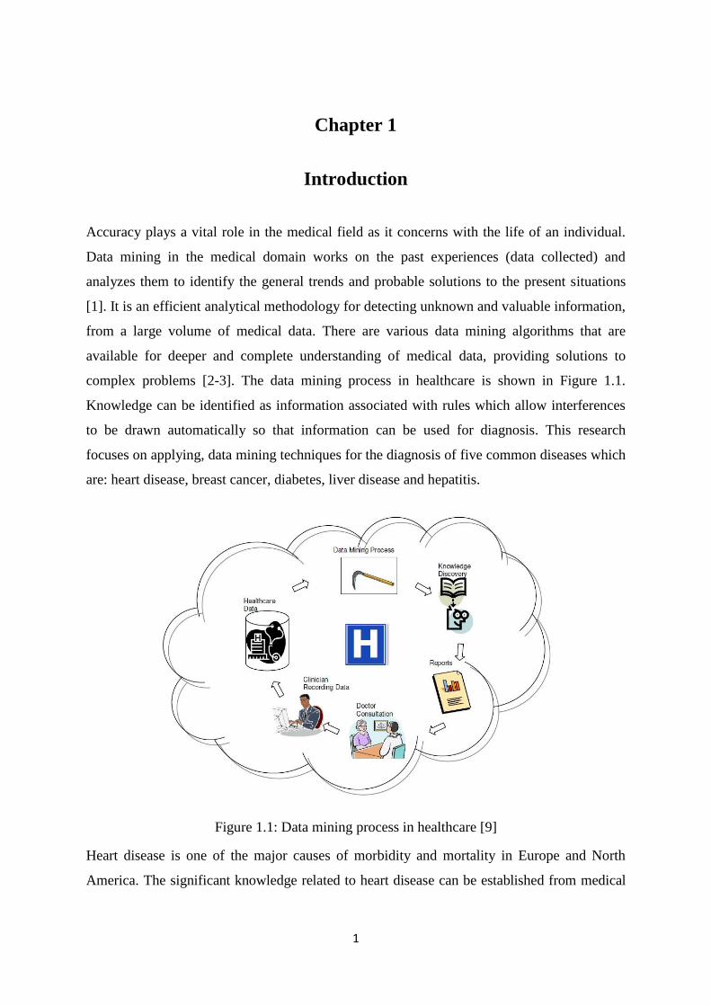
Accuracy plays a vital role in the medical field as it concerns with the life of an individual.
Data mining in the medical domain works on the past experiences (data collected) and
analyzes them to identify the general trends and probable solutions to the present situations
[1]. It is an efficient analytical methodology for detecting unknown and valuable information,
from a large volume of medical data. There are various data mining algorithms that are
available for deeper and complete understanding of medical data, providing solutions to
complex problems [2-3]. The data mining process in healthcare is shown in Figure 1.1.
Knowledge can be identified as information associated with rules which allow interferences
to be drawn automatically so that information can be used for diagnosis. This research
focuses on applying, data mining techniques for the diagnosis of five common diseases which
are: heart disease, breast cancer, diabetes, liver disease and hepatitis.
Figure 1.1: Data mining process in healthcare [9]
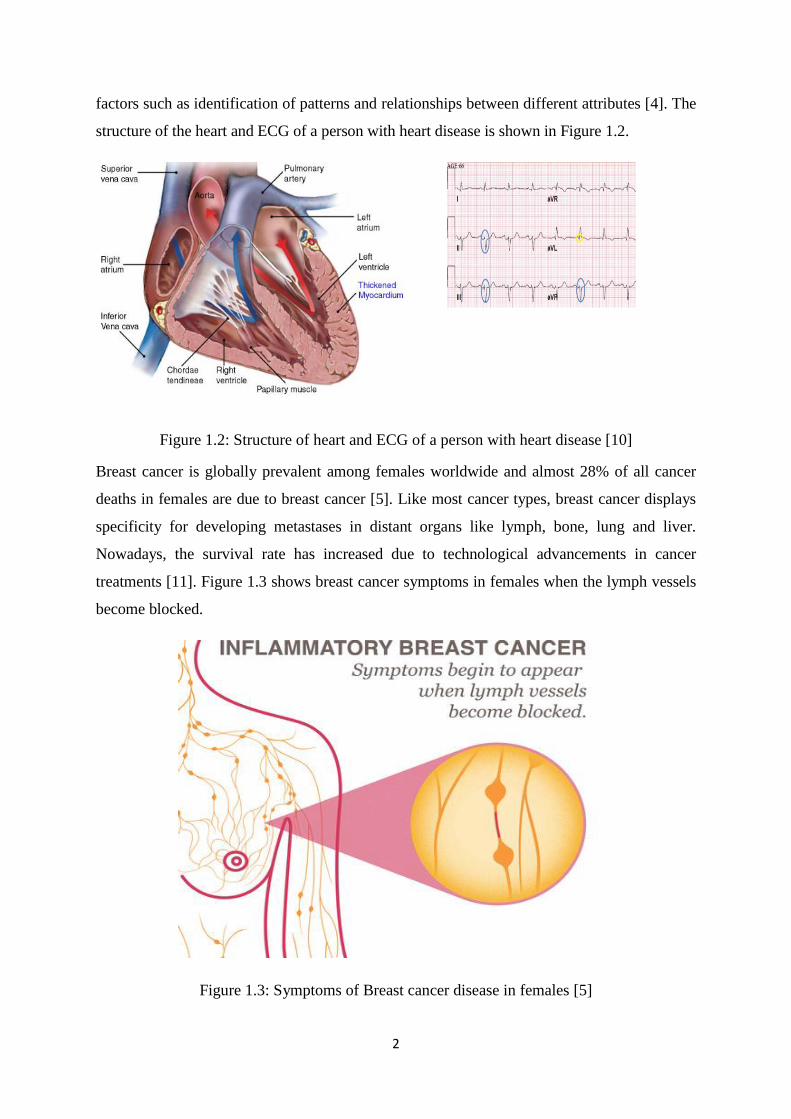
Heart disease is one of the major causes of morbidity and mortality in Europe and North
America. The significant knowledge related to heart disease can be established from medical
2
factors such as identification of patterns and relationships between different attributes [4]. The
structure of the heart and ECG of a person with heart disease is shown in Figure 1.2.
Figure 1.2: Structure of heart and ECG of a person with heart disease [10]
Breast cancer is globally prevalent among females worldwide and almost 28% of all cancer
deaths in females are due to breast cancer [5]. Like most cancer types, breast cancer displays
specificity for developing metastases in distant organs like lymph, bone, lung and liver.
Nowadays, the survival rate has increased due to technological advancements in cancer
treatments [11]. Figure 1.3 shows breast cancer symptoms in females when the lymph vessels
become blocked.
Figure 1.3: Symptoms of Breast cancer disease in females [5]
3
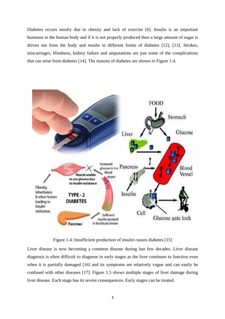
Diabetes occurs mostly due to obesity and lack of exercise [6]. Insulin is an important
hormone in the human body and if it is not properly produced then a large amount of sugar is
driven out from the body and results in different forms of diabetes [12], [13]. Strokes,
miscarriages, blindness, kidney failure and amputations are just some of the complications
that can arise from diabetes [14]. The reasons of diabetes are shown in Figure 1.4.
Figure 1.4: Insufficient production of insulin causes diabetes [15]
Liver disease is now becoming a common disease during last few decades. Liver disease
diagnosis is often difficult to diagnose in early stages as the liver continues to function even
when it is partially damaged [16] and its symptoms are relatively vague and can easily be
confused with other diseases [17]. Figure 1.5 shows multiple stages of liver damage during
liver disease. Each stage has its severe consequences. Early stages can be treated.

4
Figure 1.5: Various stages of liver damage during liver disease [18]
Hepatitis means injury to the liver with inflammation of the liver cells. There are five main
types of hepatitis, i.e., A, B, C, D and E plus type X and G. Many people with hepatitis
experience mild symptoms or none at all. At the initial phase of hepatitis, a patient suffers
from mild flu, diarrhea, fatigue, loss of appetite and mild fever etc. If the proper medication is
not adopted, then it can be developed into the fulminant or rapidly progressing form, which
can lead to death. There are multiple treatment plans for each type of hepatitis such as
hepatitis A can be treated by avoiding alcohol and drugs, the hepatitis B patient requires a
diet with high protein. Hepatitis C is treated by taking vitamin B12 supplements, whereas
there is no effective treatment for hepatitis D and E [19]. Different types of hepatitis virus are
shown in Figure 1.6.
Figure 1.6: Structure of hepatitis A, B, C, D and E virus [20]
5
1.1 Data Mining and Machine Learning
In recent years, Data Mining (DM) and Knowledge Discovery in Databases (KDD) have
become one of the most valuable tools for extracting data and for establishing patterns in
order to produce useful information for decision making. The tremendous amount of data that
is stored in large and multiple data repositories has far exceeded our human ability for
comprehension without powerful tools. This situation results in data archives where a large
volume of data is collected in data repositories which is rarely visited. Consequently,
important decisions are often made, based not on the information-rich data stored in data
repositories, but on a decision maker‘s intuition, simply because the decision maker does not
have the tools to extract the valuable knowledge embedded in the vast amounts of data. Data
mining can uncover hidden patterns in data, contributing greatly to business strategies,
knowledge bases and scientific modeling and medical research [21].
There are a variety of names that are historically used for discovering hidden information
from a large volume of database such as data mining, information harvesting, data archiving,
knowledge discovery, data pattern processing, but recently data mining and KDD are most
commonly used in the fields of classification and prediction [22]. KDD is the process that
can be used for discovery, exploratory analysis and modeling of large data repositories [23].
Giudici, P [24] defined data mining as ―The process of selection, exploration, and modeling
of large quantities of data to discover regularities or relations that are at first unknown with
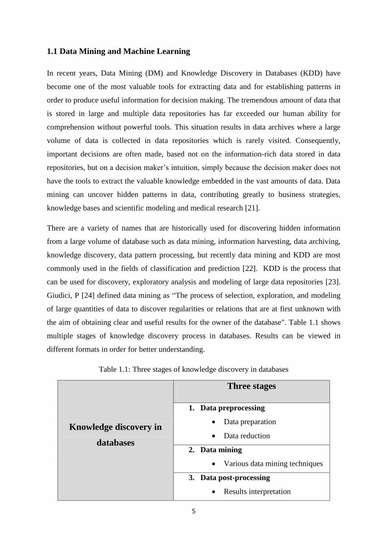
the aim of obtaining clear and useful results for the owner of the database". Table 1.1 shows
multiple stages of knowledge discovery process in databases. Results can be viewed in
different formats in order for better understanding.
Table 1.1: Three stages of knowledge discovery in databases
Knowledge discovery in
databases
Three stages
1. Data preprocessing
Data preparation
Data reduction
2. Data mining
Various data mining techniques
3. Data post-processing
Results interpretation

6
Data mining can be basically divided into two categories: predictive data mining and
descriptive data mining [1]. Predictive data mining learns from the past experiences and
applies the learned knowledge to present situations [25]. Descriptive data mining is used to
identify hidden patterns or relationships in a dataset. The data is summarized in convenient
ways that will lead to better understanding of the way things work. The basic difference
between predictive model and descriptive model is that, a descriptive model is used to
identify properties of a given data, not to predict new properties. In contrast, the predictive
model is inferences about current data in order to make predictions. The predictive data
mining model will be the focus of this research work.
1.2 Motivation
The major challenge that the healthcare organizations are facing is provision of quality
services. Quality service corresponds to diagnosing a patient accurately and then providing
proper treatment. The main motivation of this research is to transform data into useful
information, which can help practitioners to make intelligent clinical decisions, reduce
medical errors and enhance patient safety. The proposed research will focus on heart disease,
breast cancer, diabetes, liver and hepatitis disease prediction. Whilst human decision-making
performance can be suboptimal and deteriorate as the complexity of the problem increases,
the proposed solution can help healthcare professionals to make correct decisions.
1.3 Challenges in Health Sector
1.3.1 Large Volume of Medical Data
Clinical databases are very large with hundreds of tables and fields, millions of records. The
huge amounts of data generated is too complex and voluminous to be processed and analyzed
by traditional methods. Using data mining techniques and tools to analyze such huge amounts
of data has become increasingly essential.
1.3.2 Data Quality
Data quality is the biggest challenge of data mining in the health sector and the medical
domain. Precise and complete data are difficult to acquire. Health data is often complex and
heterogeneous in nature because it is collected from various sources such as from the medical
reports of laboratory, from the discussion with the patient or from the review of physicians.
7
1.3.3 Data Privacy and Ethical issue
Data privacy is also one of the major issue in healthcare because patients do not want to
disclose their health data and personal information. This poses hurdle in disease classification
and prediction in the health sector. The hospitals that wish to maintain the data warehouses
are concerned about the privacy of patients.
1.3.4 Expensive Implementation of Data Warehousing
It is essential to collect and combine the data from different sources into a central data
warehouse before applying data mining techniques. It is also costly and time consuming
process. Small sized hospital cannot afford such huge expense of implementing data
warehousing.
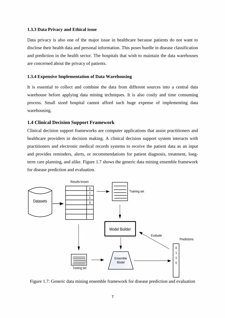
1.4 Clinical Decision Support Framework
Clinical decision support frameworks are computer applications that assist practitioners and
healthcare providers in decision making. A clinical decision support system interacts with
practitioners and electronic medical records systems to receive the patient data as an input
and provides reminders, alerts, or recommendations for patient diagnosis, treatment, long-
term care planning, and alike. Figure 1.7 shows the generic data mining ensemble framework
for disease prediction and evaluation.
Datasets
0
1
1
0
Model Builder
0
1
0
1
Results known
Training set
EvaluatePredictions
Testing set
Ensemble
Model
Figure 1.7: Generic data mining ensemble framework for disease prediction and evaluation
8
The ensemble method, combine multiple predictive models to improve the overall accuracy
of classification and regression model. The medical datasets with known class labels are
partitioned into training set and testing set. The training set is used to train the classifiers.
These trained classifiers are then combined using an ensemble technique resulting in the
construction of an ensemble model. This ensemble model is then executed on the test set and
prediction is obtained. Finally, these predicted results are compared with the results of
individual classifiers and performance is evaluated.
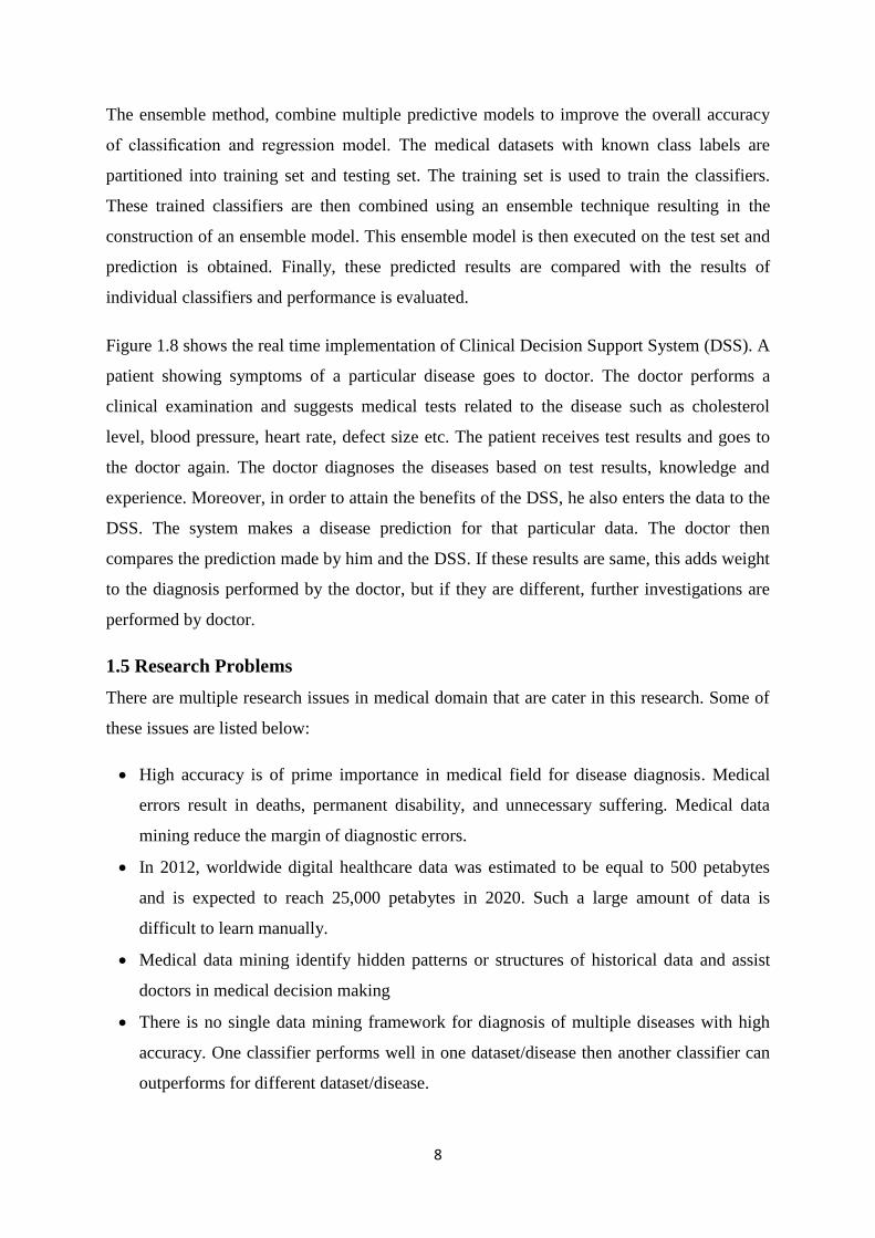
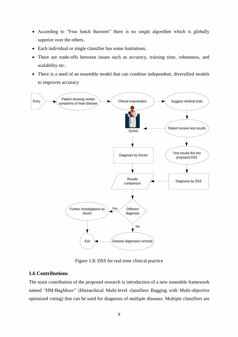
Figure 1.8 shows the real time implementation of Clinical Decision Support System (DSS). A
patient showing symptoms of a particular disease goes to doctor. The doctor performs a
clinical examination and suggests medical tests related to the disease such as cholesterol
level, blood pressure, heart rate, defect size etc. The patient receives test results and goes to
the doctor again. The doctor diagnoses the diseases based on test results, knowledge and
experience. Moreover, in order to attain the benefits of the DSS, he also enters the data to the
DSS. The system makes a disease prediction for that particular data. The doctor then
compares the prediction made by him and the DSS. If these results are same, this adds weight
to the diagnosis performed by the doctor, but if they are different, further investigations are
performed by doctor.
1.5 Research Problems
There are multiple research issues in medical domain that are cater in this research. Some of
these issues are listed below:
High accuracy is of prime importance in medical field for disease diagnosis. Medical
errors result in deaths, permanent disability, and unnecessary suffering. Medical data
mining reduce the margin of diagnostic errors.
In 2012, worldwide digital healthcare data was estimated to be equal to 500 petabytes
and is expected to reach 25,000 petabytes in 2020. Such a large amount of data is
difficult to learn manually.
Medical data mining identify hidden patterns or structures of historical data and assist
doctors in medical decision making
There is no single data mining framework for diagnosis of multiple diseases with high
accuracy. One classifier performs well in one dataset/disease then another classifier can
outperforms for different dataset/disease.
9
According to ―Free lunch theorem‖ there is no single algorithm which is globally
superior over the others.
Each individual or single classifier has some limitations.
There are trade-offs between issues such as accuracy, training time, robustness, and
scalability etc.
There is a need of an ensemble model that can combine independent, diversified models
to improves accuracy
EntryPatient showing certain
symptoms of heart diseaseClinical examination Suggest medical tests
Patient receive test results
Test results fed into
proposed DSS
Diagnosis by DSS
Diagnosis by Doctor
Doctor
Results
comparison
Different
diagnosis
Further investigations by
doctor
Disease diagnosed correctlyExit
Yes
No
Figure 1.8: DSS for real-time clinical practice
1.6 Contributions
The main contribution of the proposed research is introduction of a new ensemble framework
named "HM-BagMoov‖ (Hierarchical Multi-level classifiers Bagging with Multi-objective
optimized voting) that can be used for diagnosis of multiple diseases. Multiple classifiers are
10
used at multiple layers of the proposed ensemble framework in order to enhance disease
prediction accuracy. A novel combination of heterogeneous classifiers is presented which is
comprised of Naïve Bayes, Linear Regression, Linear Discriminant Analysis, Instance based
Learner, Support Vector Machine, Artificial Neural Network Ensemble and Random Forest
at multiple layers of classification. An ensemble technique is proposed to combine the results
of these individual classifiers in order to attain maximum accuracy for disease diagnosis. The
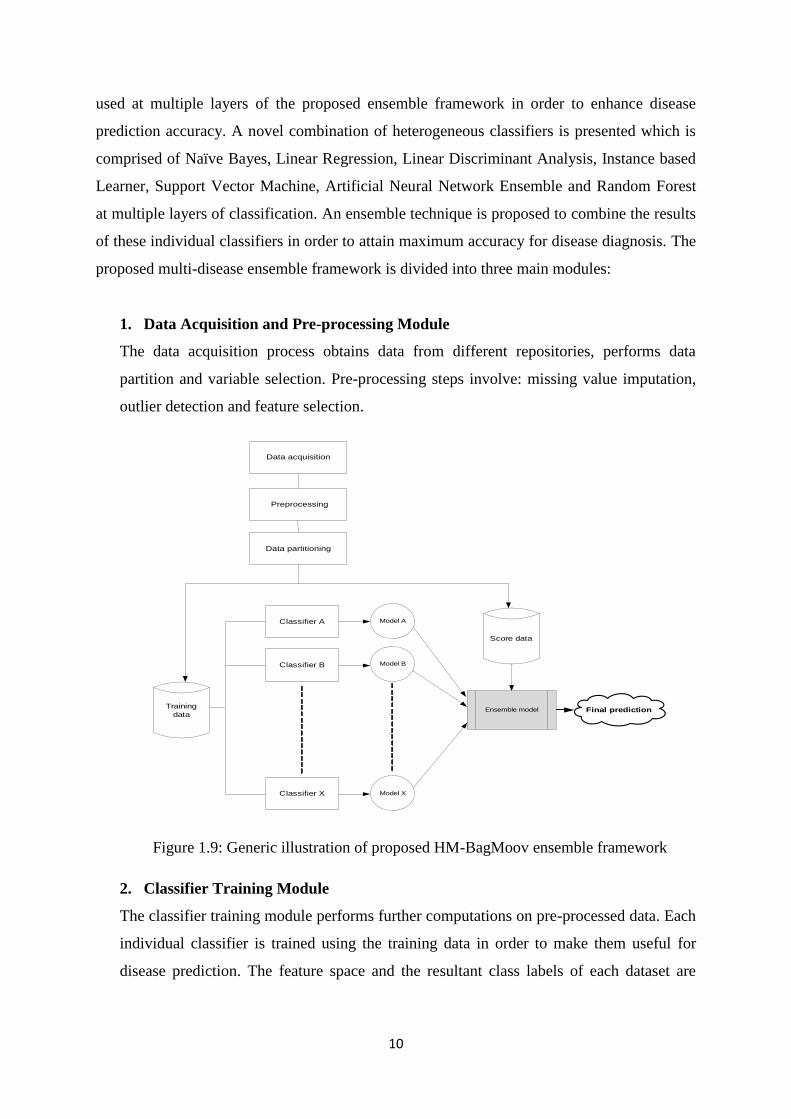
proposed multi-disease ensemble framework is divided into three main modules:
1. Data Acquisition and Pre-processing Module
The data acquisition process obtains data from different repositories, performs data
partition and variable selection. Pre-processing steps involve: missing value imputation,
outlier detection and feature selection.
Training
data
Classifier A
Classifier X
Classifier B
Model A
Model B
Model X
Ensemble model
Score data
Final prediction
Data acquisition
Preprocessing
Data partitioning
Figure 1.9: Generic illustration of proposed HM-BagMoov ensemble framework
2. Classifier Training Module
The classifier training module performs further computations on pre-processed data. Each
individual classifier is trained using the training data in order to make them useful for
disease prediction. The feature space and the resultant class labels of each dataset are

11
known to each trained classifier, which then has the capability to predict healthy and sick
individuals.
3. Prediction Algorithm
Finally, the ensemble model combines the seven individual classifiers at multiple layers.
For each classifier, the weight is calculated based on F-measure of the training dataset.
The final output of the ensemble classifier is the label with the highest weighted vote.
Figure 1.9 shows the generic diagram of proposed HM-BagMoov ensemble framework.
1.7 “IntelliHealth” Application for Disease Diagnosis
An application named ―IntelliHealth‖ has been developed for disease prediction. It is based
on proposed HM-BagMoov ensemble framework. The IntelliHealth application is also
divided into four main modules in order to maintain simplicity and efficiency. Module one is
used to enter the medical data from the user and preprocess it. Module two generates the
model using the HM-Bagmoov framework, while the third modules carries out disease
prediction. The last module is used to generate reports. The dashboard of proposed
IntelliHealth application is shown in Figure 1.10.
Figure 1.10: Proposed IntelliHealth Application
The IntelliHealth application is tested for five common diseases i.e., heart disease, breast
cancer, diabetes, liver disease and hepatitis, however it can be used for any disease
prediction. The proposed application can help both doctors and patients in terms of data
management and disease prediction.

12
1.8 Organization of the thesis
The rest of this thesis is structured as follows:
Chapter 2: Background
Chapter two presents a detailed description of multiple data mining techniques and ensemble
frameworks that are used for disease diagnosis In medical domain.
Chapter 3: State of the art techniques in medical domain
Chapter three provides a detailed review of the state of the art techniques used in medical
domain for classification and prediction.
Chapter 4: Research Methodology
Chapter four discusses the research methodology, which includes multiple ensemble
frameworks that are proposed for diseases prediction. Moreover, multi-layer, multi disease
HM-BagMoov ensemble framework is also described in detail along with the preprocessing
techniques.
Chapter 5: Experimental Results
Details of the datasets used for evaluation purposes are given in chapter five. This is then
followed by evaluation and analysis of the results. The comparison results with other state of
the art techniques are also given in this chapter.
Chapter 6: IntelliHealth: An Intelligent Application for Disease Diagnosis
Chapter six introduces the IntelliHealth application based on the proposed ensemble
framework for disease prediction.
Chapter 7: Conclusion and Future Work
Chapter seven contains the concluding remarks and the future work.
1.9 Summary
Knowledge discovery in databases has become one of the most valuable tools for extracting
data and for establishing patterns in order to produce useful information for decision-making
in medical data. Data mining can be divided into two categories: predictive data mining and
descriptive data mining. The predictive data mining model will be the focus of this research
work. Data mining techniques are used to aid in the development of predictive models that
enable classification and predication. This research focuses on applying machine learning
methods for the diagnosis of five common diseases.
13
Chapter 2
Background
This chapter gives a brief introduction of multiple machine learning techniques and ensemble
classifiers that can be used for disease classification and prediction. Finally it summarizes
Decision Support Systems (DSS) and examples of DSS in medical domain.
2.1 Machine Learning Methods
Machine learning is the process where sample data is used to infer rules or model which can
then be used for classification and prediction. The dependencies among data are described
and mapping of correlation between data inputs and outputs is determined.
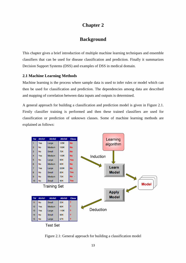
A general approach for building a classification and prediction model is given in Figure 2.1.
Firstly classifier training is performed and then these trained classifiers are used for
classification or prediction of unknown classes. Some of machine learning methods are
explained as follows:
Figure 2.1: General approach for building a classification model

14
2.1.1 Naïve Bayes (NB)
NB is extensively used for both classification and predication. Naïve Bayes algorithm
assumes that the features in the dataset are independent of each other [34].
Let X is a vector that needs to be classified and Ck be a possible class. It is necessary to
determine the probability that vector X belongs to class Ck. The probability P(Ck|X) can be
calculated using Bayesian rule:
(2.1)
The class probability P(Ck) is obtained from training data, but due to the sparseness of data,
the direct estimation of P(Ck|X) is not possible. Therefore, the P(X|Ck) can be decomposed as
follows:
∏
(2.2)
Where Xj represents the jth
element of the vector X. Combining equation (2.1) and (2.2), we
have
∏
(2.3)
The main advantage of Naïve Bayes classifier is that it requires a small amount of dataset for
training and estimation; such as, central tendency and spread of the input parameters. As the
attributes are independent of each other, only the attribute of a given class are needed to be
estimated instead of the entire covariance matrix [35]. The posterior probabilities are
calculated using the following formula:
(2.4)
The testing tuple will be classified in the class which has greater probability. The Naïve
Bayes is widely used learning algorithm for both discrete and continuous values.
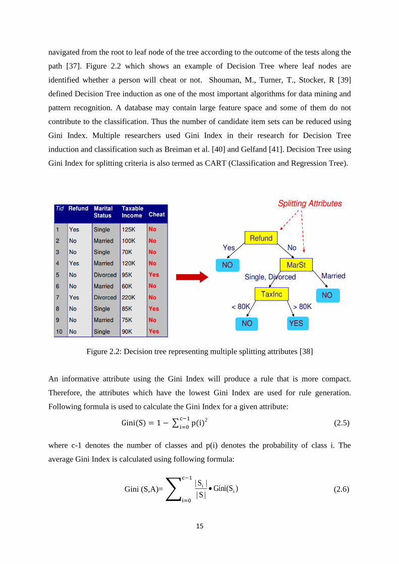
2.1.2 Decision Tree Induction based on Gini Index (DT-GI)
Decision Trees are a recursive partition of the instance space. Each leaf on a Decision Tree is
assigned to one of the output classes in target space. The instances of input space are
15
navigated from the root to leaf node of the tree according to the outcome of the tests along the
path [37]. Figure 2.2 which shows an example of Decision Tree where leaf nodes are
identified whether a person will cheat or not. Shouman, M., Turner, T., Stocker, R [39]
defined Decision Tree induction as one of the most important algorithms for data mining and
pattern recognition. A database may contain large feature space and some of them do not
contribute to the classification. Thus the number of candidate item sets can be reduced using
Gini Index. Multiple researchers used Gini Index in their research for Decision Tree
induction and classification such as Breiman et al. [40] and Gelfand [41]. Decision Tree using
Gini Index for splitting criteria is also termed as CART (Classification and Regression Tree).
Figure 2.2: Decision tree representing multiple splitting attributes [38]
An informative attribute using the Gini Index will produce a rule that is more compact.
Therefore, the attributes which have the lowest Gini Index are used for rule generation.
Following formula is used to calculate the Gini Index for a given attribute:
∑
2
(2.5)
where c-1 denotes the number of classes and p(i) denotes the probability of class i. The
average Gini Index is calculated using following formula:
Gini (S,A)= ∑ )Gini(S|S|
|S|i
i
(2.6)

16
Where A is an attribute that splits the set S into subsets Si. The crisp set of rules will be
generated along with the Decision Tree using the Gini Index as the split criterion.
2.1.3 Decision Tree Induction based on Information Gain (DT-IG)
Another Decision Tree induction method is based on Information Gain. The Decision Tree
based on Information Gain uses the entropy approach, whose ultimate purpose is to minimize
the entropy by identifying a split attribute.
Entropy for each attribute is calculated by using the formula as given by Bramer, M. [42]:
∑ (2.7)
The entropy of the entire set of attributes is calculated by weighted average over all sets using
the following formula:
k
1i|
iS|E
|S|
|i
S|A)I(S, (2.8)
Where A denotes attribute, S represents complete input space and Si is subspace. The
information gain of an attribute A is calculated by following formula:
k
1i|
iS|E
|S|
|i
S|E(S)A)I(S,E(S)A)Gain(S, (2.9)
The attribute which reduces the unorderedness is selected as splitting attribute using
Information Gain criteria. Maximizing Information Gain corresponds to minimizing entropy
because E(S) is a constant value for all attributes A. However, Decision Tree based on
Information Gain is problematic for attributes with large number of values because data is
divided into very small number of subsets. In order to avoid this situation, Decision Tree
based on Gain Ratio is used [43].
2.1.4 Decision Tree Induction based on Gain Ratio (DT-GR)
The Decision Tree induction based on Gain Ratio is also named as C4.5. The Gain Ratio
normalizes the Information Gain. Following formula is used to calculate the gain ratio for a
given attribute a:

17
S),
iEntropy(a
S),i
nGain(aInformatioS),
iaGainRatio( (2.10)
The Gain Ratio cannot be defined when the denominator is zero, i.e. there is no entropy for a
given attribute. Moreover, the Gain Ratio may tend to favor those attribute whose entropy is
very small. In order to avoid these situations, first, the Information Gain for all attributes is
calculated.
After decision tree construction, the tree pruning is performed to reduce the size of
constructed tree. Decision Trees that are too large in size are susceptible to a phenomenon
known as overfitting. In tree pruning, some branches of the tree are removed in order to
enhance the generalization capability of the tree. Multiple Decision Trees can be constructed
from same training data by using different splitting attributes. There, the choice of a splitting
attribute is very critical for a decision tree because it can lead to errors and anomalies if
splitting attribute is not selected correctly.
2.1.5 Memory based Learner (MBL)
Memory based Learner also named as instance based or case based learner works on the
principle of k Nearest Neighbor (kNN) approach. The k represents the number of neighbors
that need to be considered for class prediction. MBL is a supervised learning algorithm which
classifies the attributes based on training labels (k nearest neighbors) in the feature space. A
distance function is used to identify the nearest neighbors. Jabbar, M.A., Deekshatulu, B.L.,
Chandra, P [44] states that the type of distance function depends on the data type of selected
attributes. The kNN classifier requires three things for input:
The set of input records
Distance measure to calculate the distance between two records
The value of k, the number of nearest neighbors to consider for class prediction
The following steps allow us to classify an unknown instance:
Compute distance to all training dataset
Select k nearest neighbors
Use majority voting to identify the class labels of training instances in order to
determine the class label of unknown instance.
18
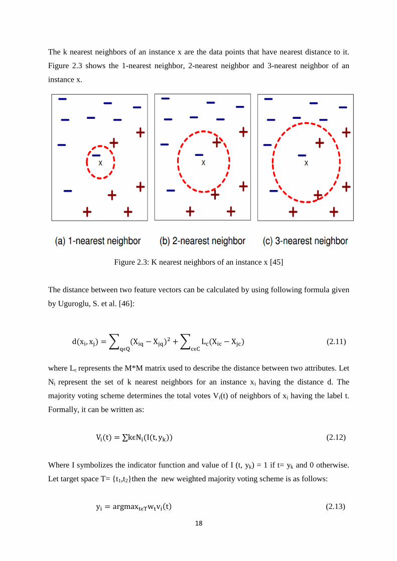
The k nearest neighbors of an instance x are the data points that have nearest distance to it.
Figure 2.3 shows the 1-nearest neighbor, 2-nearest neighbor and 3-nearest neighbor of an
instance x.
Figure 2.3: K nearest neighbors of an instance x [45]
The distance between two feature vectors can be calculated by using following formula given
by Uguroglu, S. et al. [46]:
∑
∑
(2.11)
where Lc represents the M*M matrix used to describe the distance between two attributes. Let
Ni represent the set of k nearest neighbors for an instance xi having the distance d. The
majority voting scheme determines the total votes Vi(t) of neighbors of xi having the label t.
Formally, it can be written as:
∑ (2.12)
Where I symbolizes the indicator function and value of I (t, yk) = 1 if t= yk and 0 otherwise.
Let target space T= {t1,t2}then the new weighted majority voting scheme is as follows:
(2.13)
19
The value of k and weights of class voting are selected empirically on the training set. The
following formulation of class weights is then used:
⁄ (2.14)
where w0 is the weight of majority class whereas w1 represents the minority class weight.
The MBL classifier stores all the training instances for all the available cases and classifies a
new instance based on similarity measure. It is a lazy learner where classification is deferred
until a new instance arrives. It is one of the simplest machine learning algorithms. It is a
highly effective inductive method for noisy data and complex target functions. The
shortcoming of kNN algorithm is that it is affected by the local structure of data.
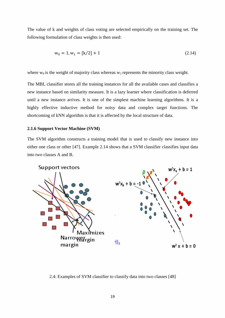
2.1.6 Support Vector Machine (SVM)
The SVM algorithm constructs a training model that is used to classify new instance into
either one class or other [47]. Example 2.14 shows that a SVM classifier classifies input data
into two classes A and B.
2.4: Examples of SVM classifier to classify data into two classes [48]

20
Generally, SVM is used for pattern classification and non-linear regression. The linear
separation is defined by; a weight vector w and bias b which represents the distance of
hyperplane from origin. Linear SVM classifies all training data using the following formula:
1
iyif1b
iwx
1i
yif1bi
wx
(2.19)
Maximize the margin by:
|w|
2M (2.20)
The advantages of SVM are:
It performs efficiently for high dimensional feature space.
It is effective in cases when the number of dimensions are higher than number of
samples.
It is memory efficient classifier because the subset of training instances is used in
decision function.
Different kernel functions can be used for different decision functions.
2.1.7 Linear Regression (LR)
Regression determines the relationship between the set of independent variables and a
dependent variable in order to perform prediction for the dependent variable. The prior
relationship identifies the future outcome [50]. A scatter plot can be used to determine the
relationship between these two variables. If the scatter plot does not show increase or
decrease in the trend of data then the correlation coefficient is used to represent the numerical
measure between independent and dependent variable. Its value ranges between -1 to 1
indicating the strength of association between two variables. The linear regression model is
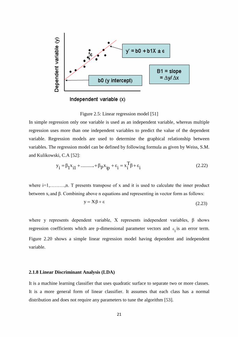
shown in Figure 2.5.
A linear regression line is represented by the following equation:
Y=a+bX (2.21)
Where X is independent variable whereas Y is dependent variable. The slope of the line is
shown with b and a is the intercept.
21
Figure 2.5: Linear regression model [51]
In simple regression only one variable is used as an independent variable, whereas multiple
regression uses more than one independent variables to predict the value of the dependent
variable. Regression models are used to determine the graphical relationship between
variables. The regression model can be defined by following formula as given by Weiss, S.M.
and Kulikowski, C.A [52]:
iεβT
ix
iε
ipxpβ...........
i1x
1β
iy (2.22)
where i=1,………,n. T presents transpose of x and it is used to calculate the inner product
between xi and β. Combining above n equations and representing in vector form as follows:
εβXy (2.23)
where y represents dependent variable, X represents independent variables, β shows
regression coefficients which are p-dimensional parameter vectors and i
ε is an error term.
Figure 2.20 shows a simple linear regression model having dependent and independent
variable.
2.1.8 Linear Discriminant Analysis (LDA)
It is a machine learning classifier that uses quadratic surface to separate two or more classes.
It is a more general form of linear classifier. It assumes that each class has a normal
distribution and does not require any parameters to tune the algorithm [53].
22
In statistical classification, suppose x is a set of vectors of an event or object and y is known
type of each vector. Now, for a new vector x, for the best class be determined, the quadratic
classifier considers quadratic measurements, where y can be determined using the following
formula:
cxTbAxTx (2.24)
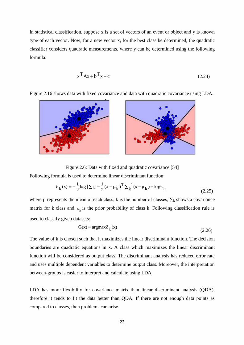
Figure 2.16 shows data with fixed covariance and data with quadratic covariance using LDA.
Figure 2.6: Data with fixed and quadratic covariance [54]
Following formula is used to determine linear discriminant function:
klogπ)
kμx1
k(T)
kμ(x
2
1k||log
2
1(x)
kδ
(2.25)
where µ represents the mean of each class, k is the number of classes, ∑k shows a covariance
matrix for k class and k
π is the prior probability of class k. Following classification rule is
used to classify given datasets:
(x)
kargmaxδG(x)
(2.26)
The value of k is chosen such that it maximizes the linear discriminant function. The decision
boundaries are quadratic equations in x. A class which maximizes the linear discriminant
function will be considered as output class. The discriminant analysis has reduced error rate
and uses multiple dependent variables to determine output class. Moreover, the interpretation
between-groups is easier to interpret and calculate using LDA.
LDA has more flexibility for covariance matrix than linear discriminant analysis (QDA),
therefore it tends to fit the data better than QDA. If there are not enough data points as
compared to classes, then problems can arise.
23
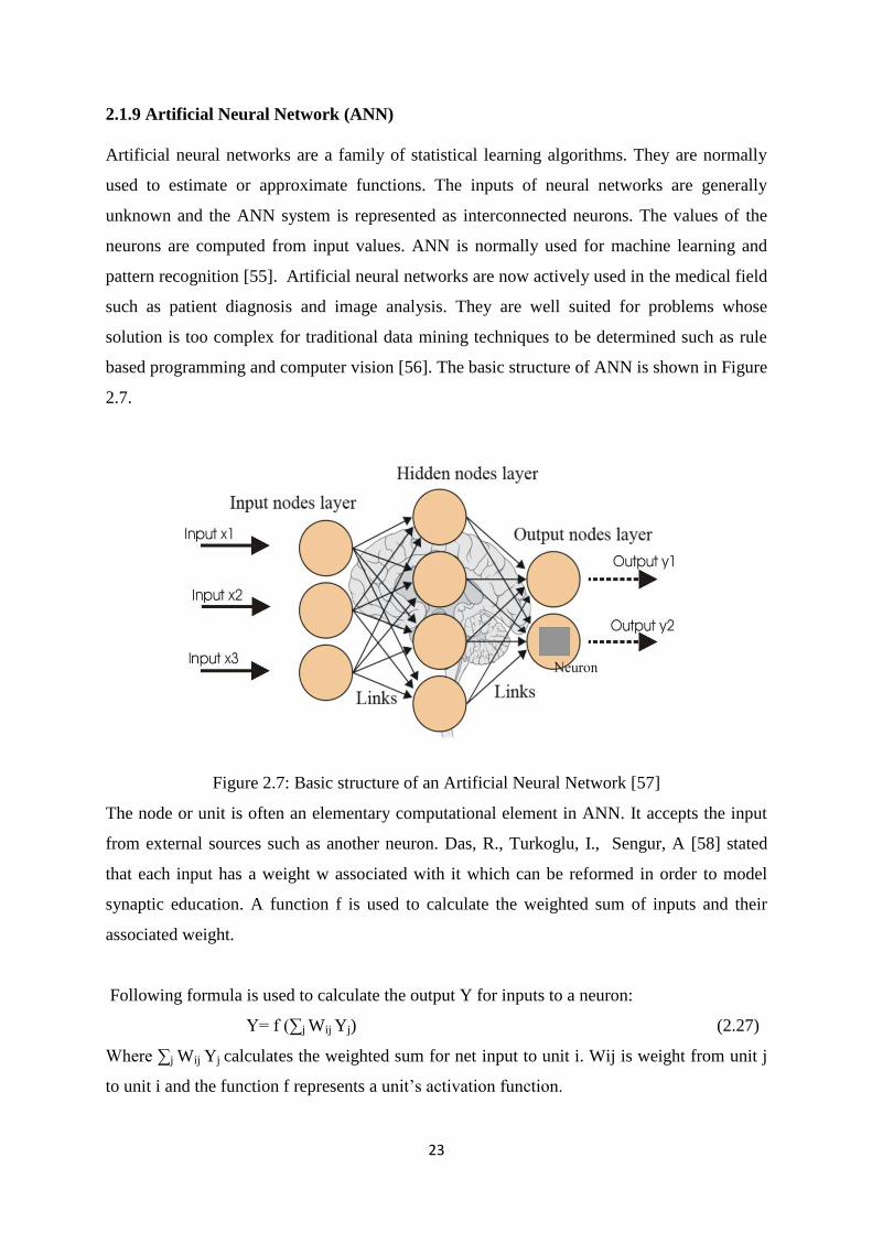
2.1.9 Artificial Neural Network (ANN)
Artificial neural networks are a family of statistical learning algorithms. They are normally
used to estimate or approximate functions. The inputs of neural networks are generally
unknown and the ANN system is represented as interconnected neurons. The values of the
neurons are computed from input values. ANN is normally used for machine learning and
pattern recognition [55]. Artificial neural networks are now actively used in the medical field
such as patient diagnosis and image analysis. They are well suited for problems whose
solution is too complex for traditional data mining techniques to be determined such as rule
based programming and computer vision [56]. The basic structure of ANN is shown in Figure
2.7.
Figure 2.7: Basic structure of an Artificial Neural Network [57]
The node or unit is often an elementary computational element in ANN. It accepts the input
from external sources such as another neuron. Das, R., Turkoglu, I., Sengur, A [58] stated
that each input has a weight w associated with it which can be reformed in order to model
synaptic education. A function f is used to calculate the weighted sum of inputs and their
associated weight.
Following formula is used to calculate the output Y for inputs to a neuron:
Y= f (∑j Wij Yj) (2.27)
Where ∑j Wij Yj calculates the weighted sum for net input to unit i. Wij is weight from unit j
to unit i and the function f represents a unit‘s activation function.
24
There are multiple applications of neural networks. They are mostly used in problems where
a function needs to be inferred from observations. It is also used in situations where the
complexity of data is very high. The neural networks tasks broadly lie in following
categories:
Function approximation or regression analysis.
Classification such as pattern recognition and novelty detection etc.
Data processing such as filtering and clustering etc.
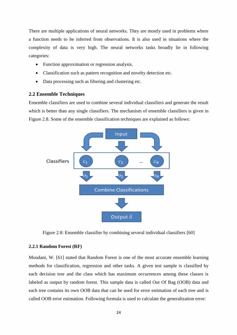
2.2 Ensemble Techniques
Ensemble classifiers are used to combine several individual classifiers and generate the result
which is better than any single classifiers. The mechanism of ensemble classifiers is given in
Figure 2.8. Some of the ensemble classification techniques are explained as follows:
Figure 2.8: Ensemble classifier by combining several individual classifiers [60]
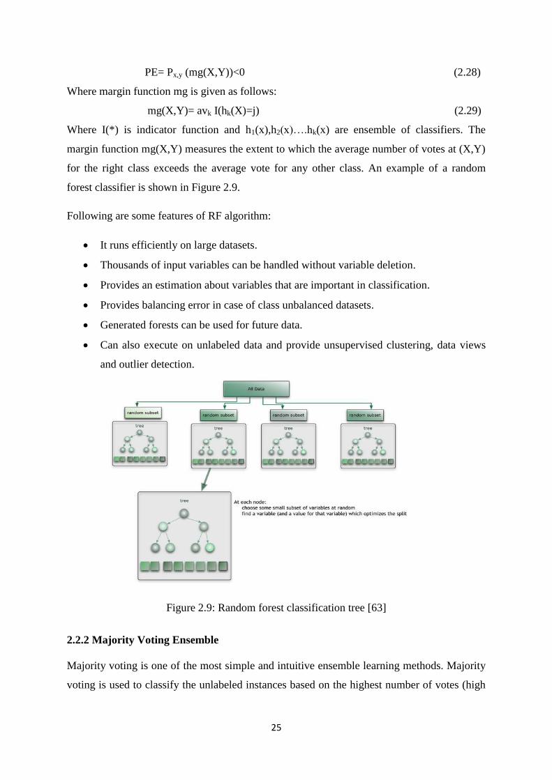
2.2.1 Random Forest (RF)
Moudani, W. [61] stated that Random Forest is one of the most accurate ensemble learning
methods for classification, regression and other tasks. A given test sample is classified by
each decision tree and the class which has maximum occurrences among these classes is
labeled as output by random forest. This sample data is called Out Of Bag (OOB) data and
each tree contains its own OOB data that can be used for error estimation of each tree and is
called OOB error estimation. Following formula is used to calculate the generalization error:
25
PE= Px,y (mg(X,Y))<0 (2.28)
Where margin function mg is given as follows:
mg(X,Y)= avk I(hk(X)=j) (2.29)
Where I(*) is indicator function and h1(x),h2(x)….hk(x) are ensemble of classifiers. The
margin function mg(X,Y) measures the extent to which the average number of votes at (X,Y)
for the right class exceeds the average vote for any other class. An example of a random
forest classifier is shown in Figure 2.9.
Following are some features of RF algorithm:
It runs efficiently on large datasets.
Thousands of input variables can be handled without variable deletion.
Provides an estimation about variables that are important in classification.
Provides balancing error in case of class unbalanced datasets.
Generated forests can be used for future data.
Can also execute on unlabeled data and provide unsupervised clustering, data views
and outlier detection.
Figure 2.9: Random forest classification tree [63]
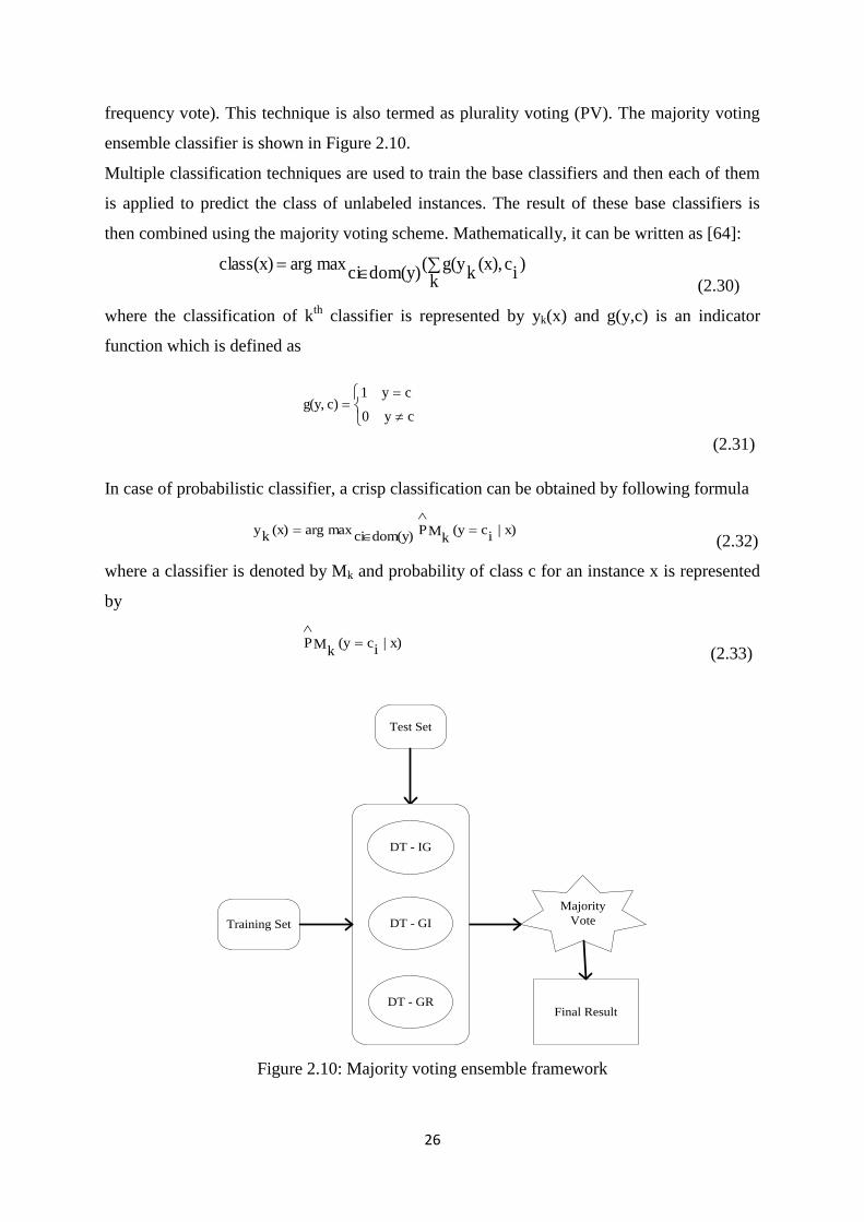
2.2.2 Majority Voting Ensemble
Majority voting is one of the most simple and intuitive ensemble learning methods. Majority
voting is used to classify the unlabeled instances based on the highest number of votes (high
26
frequency vote). This technique is also termed as plurality voting (PV). The majority voting
ensemble classifier is shown in Figure 2.10.
Multiple classification techniques are used to train the base classifiers and then each of them
is applied to predict the class of unlabeled instances. The result of these base classifiers is
then combined using the majority voting scheme. Mathematically, it can be written as [64]:
k)
ic(x),
kg(y(
dom(y)cimaxargclass(x)
(2.30)
where the classification of kth
classifier is represented by yk(x) and g(y,c) is an indicator
function which is defined as
cy0
cy1c)g(y,
(2.31)
In case of probabilistic classifier, a crisp classification can be obtained by following formula
x)|
ic(y
kMP
dom(y)cimaxarg(x)
ky
(2.32)
where a classifier is denoted by Mk and probability of class c for an instance x is represented
by
x)|
ic(y
kMP
(2.33)
Training Set
Test Set
Majority
Vote
Final Result
DT - IG
DT - GR
DT - GI
Figure 2.10: Majority voting ensemble framework

27
2.2.3 Bagging Ensemble
Bagging is a ―Bootstrap‖ ensemble method and also termed as Bootstrap Aggregation. In
Figure 2.11 assume there are eight training samples. With bagging approach, some of the
samples are repeated in training sets while some are left out.
Figure 2.11: Hypothetical runs of Bagging
The outputs of individual classifiers are combined to generate a final output class. Breiman,
L. [66] proved that bagging can perform better as compared to individual classifiers because
bagging can eliminate the instability of single inducers. A voting approach is used to combine
the results of individual classifiers. Bagging ensemble classifier is shown in Figure 2.12.
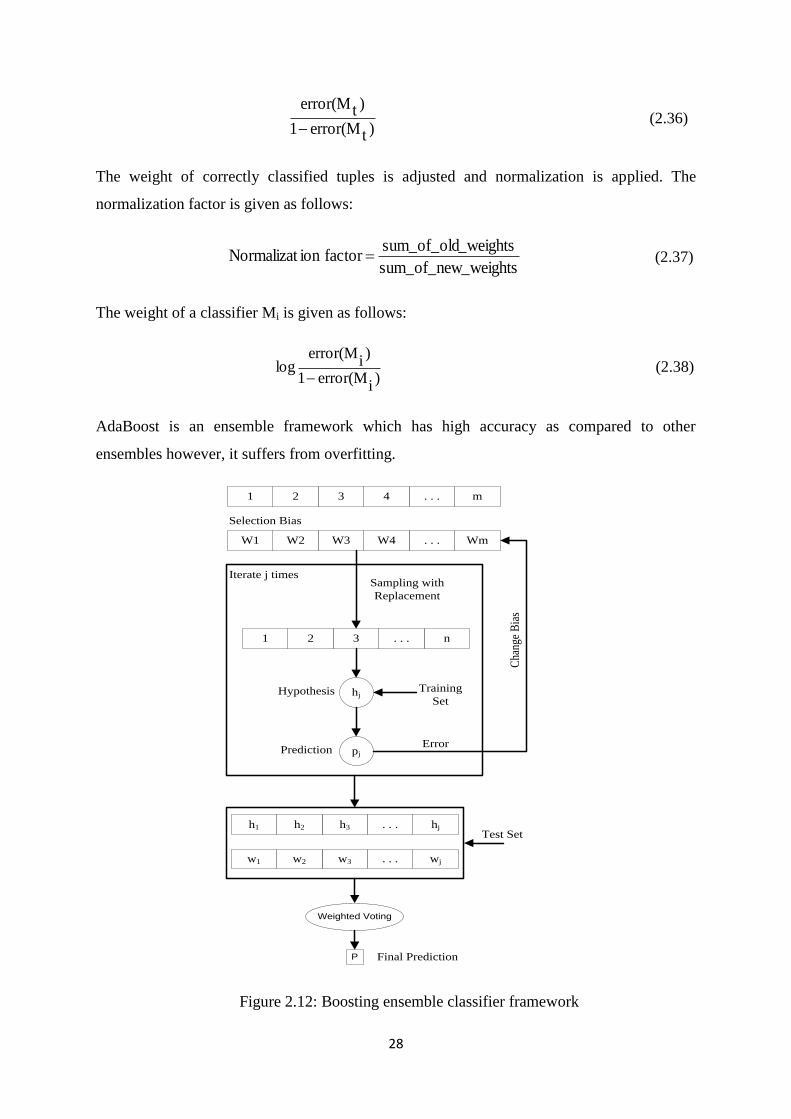
2.2.4 AdaBoost Ensemble
AdaBoost is a popular ensemble algorithm introduced by Maroco, J. et al. [67] and it is the
most frequently used algorithm among all boosting algorithms. Boosting ensemble classifier
is shown in Fig 2.23. Maroco, J. et al. [67] stated that mathematically, the AdaBoost
ensemble method can be written as:
(x))tM
T
1t.tαsign(H(x)
(2.34)
where Mt denotes the classification based on voting of all classifiers for a particular instance
and tα is weight. The error rate of model Mt is determined by following formula:
d
j)
jerror(X*
jw)terror(M (2.35)
Where error(Xj) is misclassification error for Xj=1.
If a tuple is correctly classified in round i then its weight is multiplied by:
28
)terror(M1
)terror(M
(2.36)
The weight of correctly classified tuples is adjusted and normalization is applied. The
normalization factor is given as follows:
_weightssum_of_new
_weightssum_of_oldfactorionNormalizat (2.37)
The weight of a classifier Mi is given as follows:
)
ierror(M1
)i
error(Mlog
(2.38)
AdaBoost is an ensemble framework which has high accuracy as compared to other
ensembles however, it suffers from overfitting.
m. . .4321
Wm. . .W4W3W2W1
Selection Bias
n. . .321
Sampling with
Replacement
hjHypothesis Training
Set
pjPredictionError
Cha
nge
Bia
s
Iterate j times
hj. . .h3h2h1
wj. . .w3w2w1
Test Set
Weighted Voting
P Final Prediction
Figure 2.12: Boosting ensemble classifier framework
29
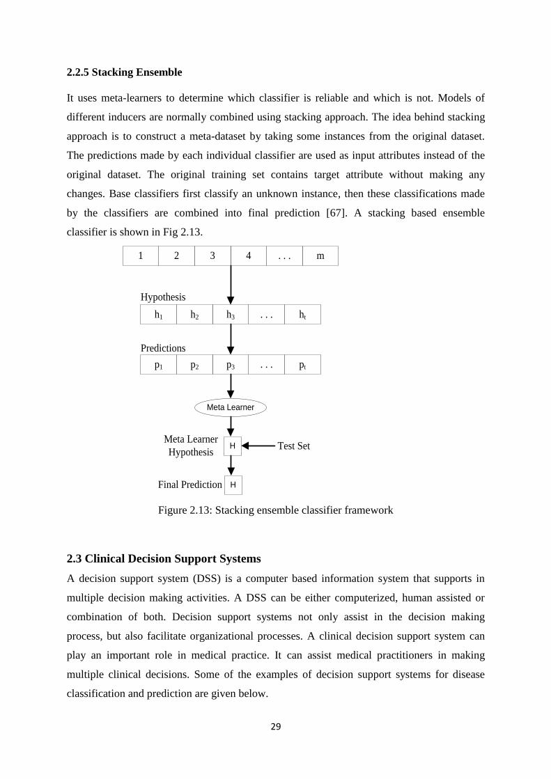
2.2.5 Stacking Ensemble
It uses meta-learners to determine which classifier is reliable and which is not. Models of
different inducers are normally combined using stacking approach. The idea behind stacking
approach is to construct a meta-dataset by taking some instances from the original dataset.
The predictions made by each individual classifier are used as input attributes instead of the
original dataset. The original training set contains target attribute without making any
changes. Base classifiers first classify an unknown instance, then these classifications made
by the classifiers are combined into final prediction [67]. A stacking based ensemble
classifier is shown in Fig 2.13.
m. . .4321
ht. . .h3h2h1
pt. . .p3p2p1
Meta Learner
HMeta Learner
Hypothesis
Hypothesis
Predictions
Test Set
HFinal Prediction
Figure 2.13: Stacking ensemble classifier framework
2.3 Clinical Decision Support Systems
A decision support system (DSS) is a computer based information system that supports in
multiple decision making activities. A DSS can be either computerized, human assisted or
combination of both. Decision support systems not only assist in the decision making
process, but also facilitate organizational processes. A clinical decision support system can
play an important role in medical practice. It can assist medical practitioners in making
multiple clinical decisions. Some of the examples of decision support systems for disease
classification and prediction are given below.
30
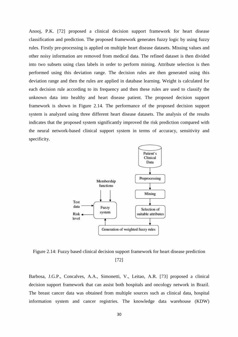
Anooj, P.K. [72] proposed a clinical decision support framework for heart disease
classification and prediction. The proposed framework generates fuzzy logic by using fuzzy
rules. Firstly pre-processing is applied on multiple heart disease datasets. Missing values and
other noisy information are removed from medical data. The refined dataset is then divided
into two subsets using class labels in order to perform mining. Attribute selection is then
performed using this deviation range. The decision rules are then generated using this
deviation range and then the rules are applied in database learning. Weight is calculated for
each decision rule according to its frequency and then these rules are used to classify the
unknown data into healthy and heart disease patient. The proposed decision support
framework is shown in Figure 2.14. The performance of the proposed decision support
system is analyzed using three different heart disease datasets. The analysis of the results
indicates that the proposed system significantly improved the risk prediction compared with
the neural network-based clinical support system in terms of accuracy, sensitivity and
specificity.
Figure 2.14: Fuzzy based clinical decision support framework for heart disease prediction
[72]
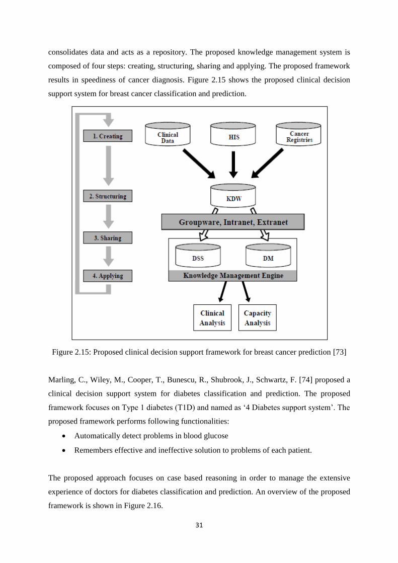
Barbosa, J.G.P., Concalves, A.A., Simonetti, V., Leitao, A.R. [73] proposed a clinical
decision support framework that can assist both hospitals and oncology network in Brazil.
The breast cancer data was obtained from multiple sources such as clinical data, hospital
information system and cancer registries. The knowledge data warehouse (KDW)
31
consolidates data and acts as a repository. The proposed knowledge management system is
composed of four steps: creating, structuring, sharing and applying. The proposed framework
results in speediness of cancer diagnosis. Figure 2.15 shows the proposed clinical decision
support system for breast cancer classification and prediction.
Figure 2.15: Proposed clinical decision support framework for breast cancer prediction [73]
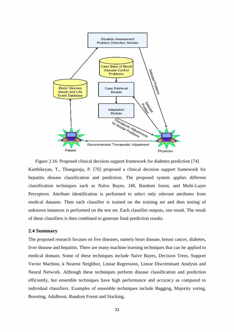
Marling, C., Wiley, M., Cooper, T., Bunescu, R., Shubrook, J., Schwartz, F. [74] proposed a
clinical decision support system for diabetes classification and prediction. The proposed
framework focuses on Type 1 diabetes (T1D) and named as ‗4 Diabetes support system‘. The
proposed framework performs following functionalities:
Automatically detect problems in blood glucose
Remembers effective and ineffective solution to problems of each patient.
The proposed approach focuses on case based reasoning in order to manage the extensive
experience of doctors for diabetes classification and prediction. An overview of the proposed
framework is shown in Figure 2.16.
32
Figure 2.16: Proposed clinical decision support framework for diabetes prediction [74]
Karthikeyan, T., Thangaraju, P. [76] proposed a clinical decision support framework for
hepatitis disease classification and prediction. The proposed system applies different
classification techniques such as Naïve Bayes, J48, Random forest, and Multi-Layer
Perceptron. Attribute identification is performed to select only relevant attributes from
medical datasets. Then each classifier is trained on the training set and then testing of
unknown instances is performed on the test set. Each classifier outputs, one result. The result
of these classifiers is then combined to generate final prediction results.
2.4 Summary
The proposed research focuses on five diseases, namely heart disease, breast cancer, diabetes,
liver disease and hepatitis. There are many machine learning techniques that can be applied to
medical domain. Some of these techniques include Naïve Bayes, Decision Trees, Support
Vector Machine, k Nearest Neighbor, Linear Regression, Linear Discriminant Analysis and
Neural Network. Although these techniques perform disease classification and prediction
efficiently, but ensemble techniques have high performance and accuracy as compared to
individual classifiers. Examples of ensemble techniques include Bagging, Majority voting,
Boosting, AdaBoost, Random Forest and Stacking.
33
Chapter 3
State of the Art Techniques in Medical Domain
Extensive amount of work has already been done on disease classification and prediction.
Some of these techniques are given in this section. In order to summarize the information, we
have focused on five diseases, i.e., heart disease, breast cancer, diabetes, liver disease and
thyroid disease.
3.1 Heart Disease Classification & Prediction
In the last few decades, multiple machine learning techniques have been widely accepted for
intelligent heart disease prediction. Table 3.1 shows a comparison of different techniques
used on heart disease datasets. It can be seen from table 1 that the current work focuses on
applying a single classifier for heart disease prediction.
Table 3.1: Machine learning techniques applied on heart disease datasets
Author/Year/Reference Technique Accuracy
Thenmozhi, K. et al., 2014 [77]
K-Mean based on MAFIA 74%
K-Mean based on MAFIA with ID3 85%
K-Mean based on MAFIA with ID3
and C4.5 92%
Chitra, R., et al., 2013 [78] Cascaded Neural Network 85%
Support Vector Machine 82%
Shouman, M., et al., 2013 [79]
Gain ratio Decision Tree 79.1%
Naïve Bayes 83.5%
K Nearest Neighbor 83.2%
Shouman, M., et al., 2012 [80] K mean clustering with Naïve
Bayes algorithm 78.62%
Ghumbre, S., et al., 2011[81] Support Vector Machine 85.05%
Radial Basis Function 82.24%
Shouman, M., et al., 2011 [82]
Nine Voting Equal Frequency
Discretization Gain Ratio Decision
Tree
84.1%
Chen, AH., et al., 2011 [83] Artificial Neural Network 80%
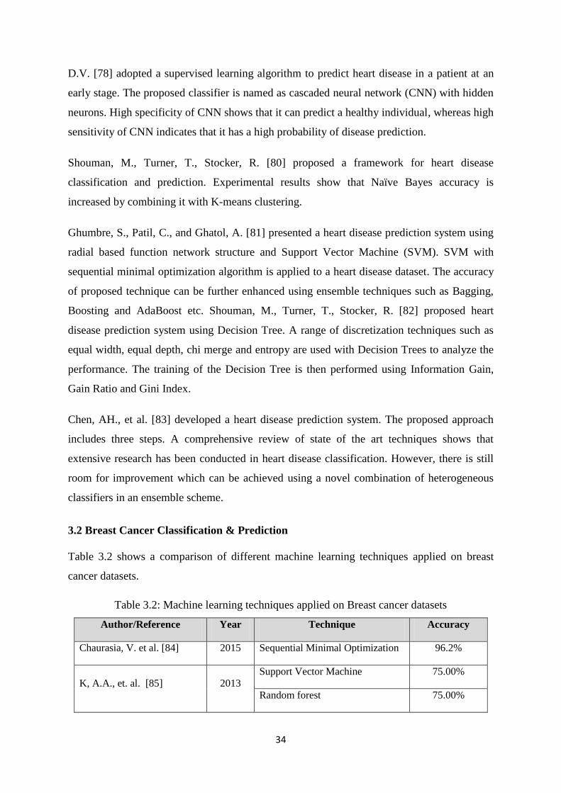
34
D.V. [78] adopted a supervised learning algorithm to predict heart disease in a patient at an
early stage. The proposed classifier is named as cascaded neural network (CNN) with hidden
neurons. High specificity of CNN shows that it can predict a healthy individual, whereas high
sensitivity of CNN indicates that it has a high probability of disease prediction.
Shouman, M., Turner, T., Stocker, R. [80] proposed a framework for heart disease
classification and prediction. Experimental results show that Naïve Bayes accuracy is
increased by combining it with K-means clustering.
Ghumbre, S., Patil, C., and Ghatol, A. [81] presented a heart disease prediction system using
radial based function network structure and Support Vector Machine (SVM). SVM with
sequential minimal optimization algorithm is applied to a heart disease dataset. The accuracy
of proposed technique can be further enhanced using ensemble techniques such as Bagging,
Boosting and AdaBoost etc. Shouman, M., Turner, T., Stocker, R. [82] proposed heart
disease prediction system using Decision Tree. A range of discretization techniques such as
equal width, equal depth, chi merge and entropy are used with Decision Trees to analyze the
performance. The training of the Decision Tree is then performed using Information Gain,
Gain Ratio and Gini Index.
Chen, AH., et al. [83] developed a heart disease prediction system. The proposed approach
includes three steps. A comprehensive review of state of the art techniques shows that
extensive research has been conducted in heart disease classification. However, there is still
room for improvement which can be achieved using a novel combination of heterogeneous
classifiers in an ensemble scheme.
3.2 Breast Cancer Classification & Prediction
Table 3.2 shows a comparison of different machine learning techniques applied on breast
cancer datasets.
Table 3.2: Machine learning techniques applied on Breast cancer datasets
Author/Reference Year Technique Accuracy
Chaurasia, V. et al. [84] 2015 Sequential Minimal Optimization 96.2%
K, A.A., et. al. [85] 2013 Support Vector Machine 75.00%
Random forest 75.00%
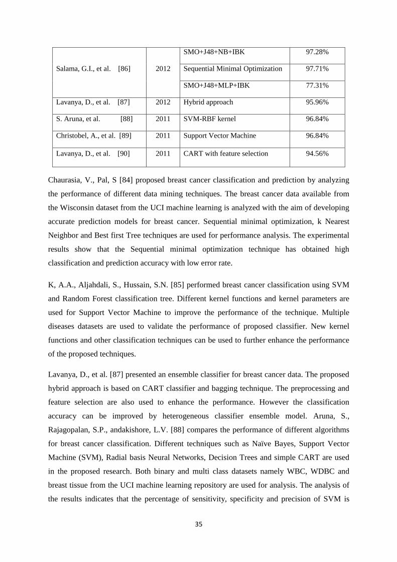
35
Salama, G.I., et al. [86] 2012
SMO+J48+NB+IBK 97.28%
Sequential Minimal Optimization 97.71%
SMO+J48+MLP+IBK 77.31%
Lavanya, D., et al. [87] 2012 Hybrid approach 95.96%
S. Aruna, et al. [88] 2011 SVM-RBF kernel 96.84%
Christobel, A., et al. [89] 2011 Support Vector Machine 96.84%
Lavanya, D., et al. [90] 2011 CART with feature selection 94.56%
Chaurasia, V., Pal, S [84] proposed breast cancer classification and prediction by analyzing
the performance of different data mining techniques. The breast cancer data available from
the Wisconsin dataset from the UCI machine learning is analyzed with the aim of developing
accurate prediction models for breast cancer. Sequential minimal optimization, k Nearest
Neighbor and Best first Tree techniques are used for performance analysis. The experimental
results show that the Sequential minimal optimization technique has obtained high
classification and prediction accuracy with low error rate.
K, A.A., Aljahdali, S., Hussain, S.N. [85] performed breast cancer classification using SVM
and Random Forest classification tree. Different kernel functions and kernel parameters are
used for Support Vector Machine to improve the performance of the technique. Multiple
diseases datasets are used to validate the performance of proposed classifier. New kernel
functions and other classification techniques can be used to further enhance the performance
of the proposed techniques.
Lavanya, D., et al. [87] presented an ensemble classifier for breast cancer data. The proposed
hybrid approach is based on CART classifier and bagging technique. The preprocessing and
feature selection are also used to enhance the performance. However the classification
accuracy can be improved by heterogeneous classifier ensemble model. Aruna, S.,
Rajagopalan, S.P., andakishore, L.V. [88] compares the performance of different algorithms
for breast cancer classification. Different techniques such as Naïve Bayes, Support Vector
Machine (SVM), Radial basis Neural Networks, Decision Trees and simple CART are used
in the proposed research. Both binary and multi class datasets namely WBC, WDBC and
breast tissue from the UCI machine learning repository are used for analysis. The analysis of
the results indicates that the percentage of sensitivity, specificity and precision of SVM is
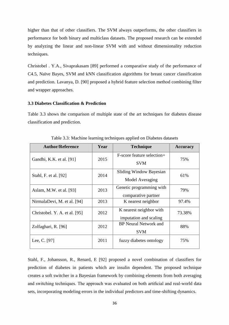
36
higher than that of other classifiers. The SVM always outperforms, the other classifiers in
performance for both binary and multiclass datasets. The proposed research can be extended
by analyzing the linear and non-linear SVM with and without dimensionality reduction
techniques.
Christobel . Y.A., Sivaprakasam [89] performed a comparative study of the performance of
C4.5, Naïve Bayes, SVM and kNN classification algorithms for breast cancer classification
and prediction. Lavanya, D. [90] proposed a hybrid feature selection method combining filter
and wrapper approaches.
3.3 Diabetes Classification & Prediction
Table 3.3 shows the comparison of multiple state of the art techniques for diabetes disease
classification and prediction.
Table 3.3: Machine learning techniques applied on Diabetes datasets
Author/Reference Year Technique Accuracy
Gandhi, K.K. et al. [91] 2015 F-score feature selection+
SVM 75%
Stahl, F. et al. [92] 2014 Sliding Window Bayesian
Model Averaging 61%
Aslam, M.W. et al. [93] 2013 Genetic programming with
comparative partner
selection
79%
NirmalaDevi, M. et al. [94] 2013 K nearest neighbor 97.4%
Christobel. Y. A. et al. [95] 2012 K nearest neighbor with
imputation and scaling 73.38%
Zolfaghari, R. [96] 2012 BP Neural Network and
SVM 88%
Lee, C. [97] 2011 fuzzy diabetes ontology 75%
Stahl, F., Johansson, R., Renard, E [92] proposed a novel combination of classifiers for
prediction of diabetes in patients which are insulin dependent. The proposed technique
creates a soft switcher in a Bayesian framework by combining elements from both averaging
and switching techniques. The approach was evaluated on both artificial and real-world data
sets, incorporating modeling errors in the individual predictors and time-shifting dynamics.
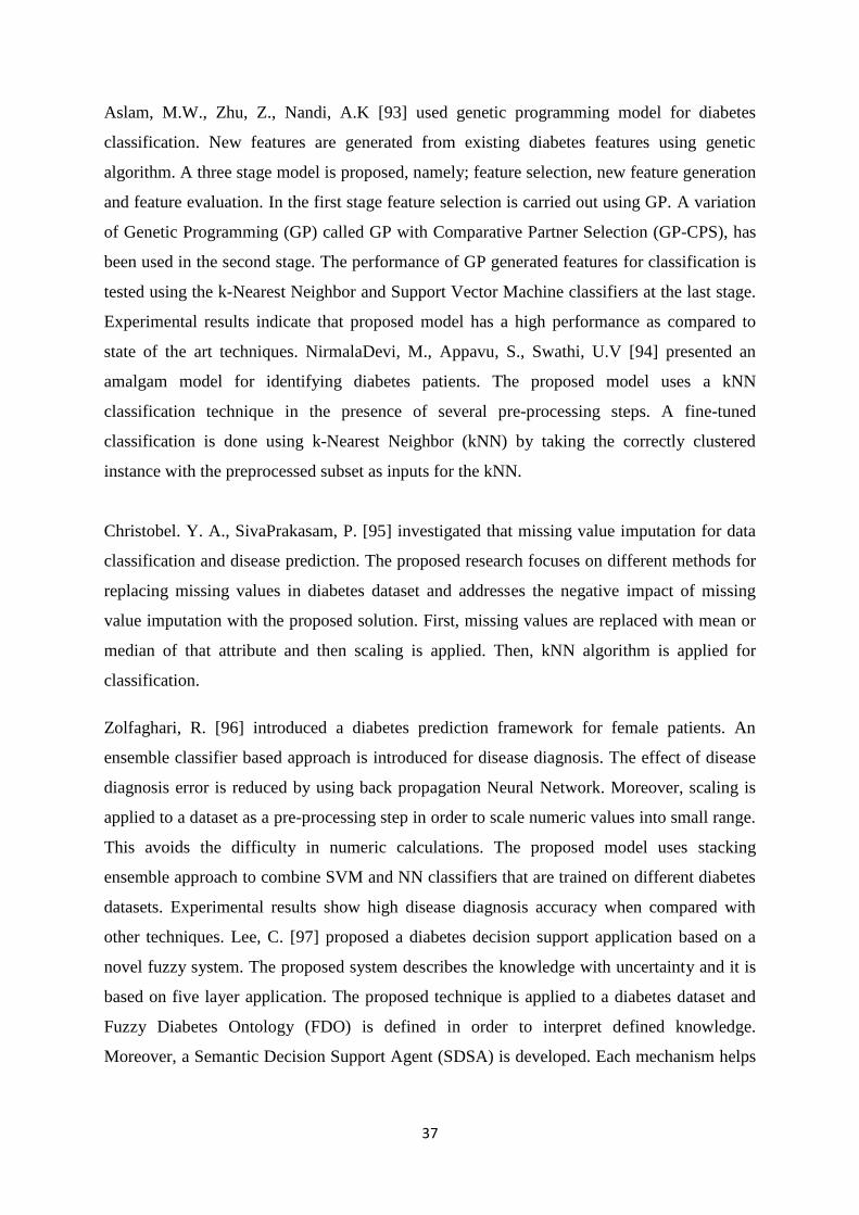
37
Aslam, M.W., Zhu, Z., Nandi, A.K [93] used genetic programming model for diabetes
classification. New features are generated from existing diabetes features using genetic
algorithm. A three stage model is proposed, namely; feature selection, new feature generation
and feature evaluation. In the first stage feature selection is carried out using GP. A variation
of Genetic Programming (GP) called GP with Comparative Partner Selection (GP-CPS), has
been used in the second stage. The performance of GP generated features for classification is
tested using the k-Nearest Neighbor and Support Vector Machine classifiers at the last stage.
Experimental results indicate that proposed model has a high performance as compared to
state of the art techniques. NirmalaDevi, M., Appavu, S., Swathi, U.V [94] presented an
amalgam model for identifying diabetes patients. The proposed model uses a kNN
classification technique in the presence of several pre-processing steps. A fine-tuned
classification is done using k-Nearest Neighbor (kNN) by taking the correctly clustered
instance with the preprocessed subset as inputs for the kNN.
Christobel. Y. A., SivaPrakasam, P. [95] investigated that missing value imputation for data
classification and disease prediction. The proposed research focuses on different methods for
replacing missing values in diabetes dataset and addresses the negative impact of missing
value imputation with the proposed solution. First, missing values are replaced with mean or
median of that attribute and then scaling is applied. Then, kNN algorithm is applied for
classification.
Zolfaghari, R. [96] introduced a diabetes prediction framework for female patients. An
ensemble classifier based approach is introduced for disease diagnosis. The effect of disease
diagnosis error is reduced by using back propagation Neural Network. Moreover, scaling is
applied to a dataset as a pre-processing step in order to scale numeric values into small range.
This avoids the difficulty in numeric calculations. The proposed model uses stacking
ensemble approach to combine SVM and NN classifiers that are trained on different diabetes
datasets. Experimental results show high disease diagnosis accuracy when compared with
other techniques. Lee, C. [97] proposed a diabetes decision support application based on a
novel fuzzy system. The proposed system describes the knowledge with uncertainty and it is
based on five layer application. The proposed technique is applied to a diabetes dataset and
Fuzzy Diabetes Ontology (FDO) is defined in order to interpret defined knowledge.
Moreover, a Semantic Decision Support Agent (SDSA) is developed. Each mechanism helps
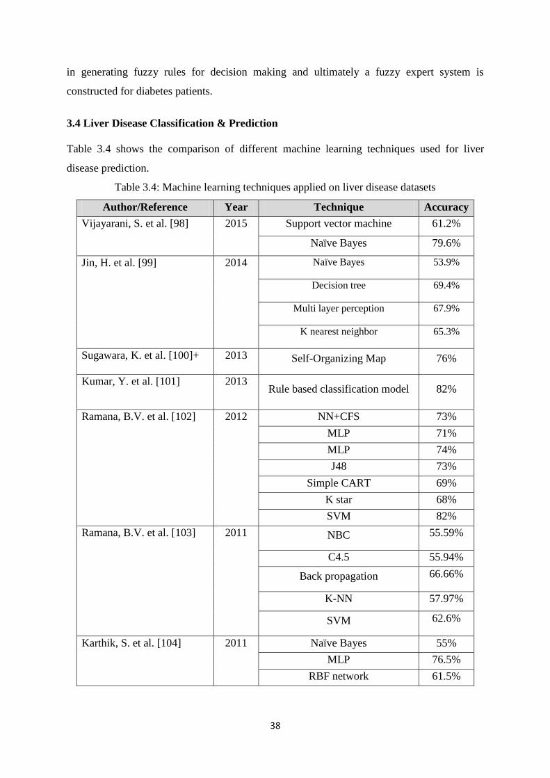
38
in generating fuzzy rules for decision making and ultimately a fuzzy expert system is
constructed for diabetes patients.
3.4 Liver Disease Classification & Prediction
Table 3.4 shows the comparison of different machine learning techniques used for liver
disease prediction.
Table 3.4: Machine learning techniques applied on liver disease datasets
Author/Reference Year Technique Accuracy
Vijayarani, S. et al. [98] 2015 Support vector machine 61.2%
Naïve Bayes 79.6%
Jin, H. et al. [99] 2014 Naïve Bayes 53.9%
Decision tree 69.4%
Multi layer perception 67.9%
K nearest neighbor 65.3%
Sugawara, K. et al. [100]+ 2013 Self-Organizing Map 76%
Kumar, Y. et al. [101] 2013 Rule based classification model 82%
Ramana, B.V. et al. [102] 2012 NN+CFS 73%
MLP 71%
MLP 74%
J48 73%
Simple CART 69%
K star 68%
SVM 82%
Ramana, B.V. et al. [103] 2011
NBC 55.59%
C4.5 55.94%
Back propagation 66.66%
K-NN 57.97%
SVM 62.6%
Karthik, S. et al. [104] 2011 Naïve Bayes 55%
MLP 76.5%
RBF network 61.5%

39
Vijayarani, S., Dhayanand, S. [98] uses different classification algorithms for diagnosis of
liver disease. Kumar, Y. and Sahoo, G. [101] proposed a Rule Based Classification Model
(RBCM) for identification and classification of different type of liver diseases. The proposed
model is combination of rule based and classification techniques. SVM, Rule Induction,
Naïve Bayes, Decision Tree and Neural Network techniques are used. The performance of
the proposed technique is evaluated using different metrics such as accuracy, sensitivity,
specificity etc. The analysis of the results indicates that Decision Tree has obtained high
classification accuracy as compared to other techniques. Ramana, B.V. et al. [102] proposed
a liver classification framework by using modified Random Forest algorithm. Different
feature selection techniques are utilized to evaluate the performance of the proposed
framework. Two liver datasets are used for experimentation. Multiple classification
algorithms are also used from each category of classification algorithms. Tree based,
Statistical based, Neural Network based, lazy learners, Rule based algorithms and Support
Vector Machine algorithms are used for classification task. A multilayer perception algorithm
along with Random Feature subset selection technique has highest classification accuracy for
the UCI liver dataset whereas k Nearest Neighbor with the combination of generalized
distance function has obtained the highest accuracy for the Indiana liver dataset. Ramana,
B.V. et al. [103] compared the accuracy, sensitivity, specificity and precision of different
classification algorithms for liver disease diagnosis. The research is based on comparing the
performance of Naive Bayes, Decision Tree (C4.5), back propagation, kNN and SVM
algorithms. The results are compared for different number of feature sets taken from liver
disease datasets and ranking algorithm is used to order the feature space. It is analyzed from
the comparison that back propagation algorithm has obtained highest classification accuracy
for the liver disease dataset. Improvements can be made by using a feature selection
algorithm for attribute reduction instead of the ranking algorithm.
3.5 Hepatitis Classification & Prediction
Various techniques that have been used for hepatitis classification and prediction. Table 3.5
shows the comparison of multiple techniques for hepatitis classification and prediction.
Table 3.5: Machine learning techniques applied on hepatitis disease datasets
Author/Reference Year Technique Accuracy
Pushpalatha, S. et al. [105] 2015 Model framework 80%
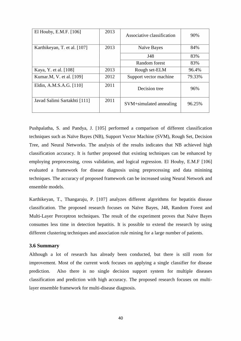
40
El Houby, E.M.F. [106] 2013 Associative classification 90%
Karthikeyan, T. et al. [107] 2013 Naïve Bayes 84%
J48 83%
Random forest 83%
Kaya, Y. et al. [108] 2013 Rough set-ELM 96.4%
Kumar.M, V. et al. [109] 2012 Support vector machine 79.33%
Eldin, A.M.S.A.G. [110] 2011 Decision tree 96%
Javad Salimi Sartakhti [111] 2011 SVM+simulated annealing 96.25%
Pushpalatha, S. and Pandya, J. [105] performed a comparison of different classification
techniques such as Naïve Bayes (NB), Support Vector Machine (SVM), Rough Set, Decision
Tree, and Neural Networks. The analysis of the results indicates that NB achieved high
classification accuracy. It is further proposed that existing techniques can be enhanced by
employing preprocessing, cross validation, and logical regression. El Houby, E.M.F [106]
evaluated a framework for disease diagnosis using preprocessing and data minining
techniques. The accuracy of proposed framework can be increased using Neural Network and
ensemble models.
Karthikeyan, T., Thangaraju, P. [107] analyzes different algorithms for hepatitis disease
classification. The proposed research focuses on Naïve Bayes, J48, Random Forest and
Multi-Layer Perceptron techniques. The result of the experiment proves that Naïve Bayes
consumes less time in detection hepatitis. It is possible to extend the research by using
different clustering techniques and association rule mining for a large number of patients.
3.6 Summary
Although a lot of research has already been conducted, but there is still room for
improvement. Most of the current work focuses on applying a single classifier for disease
prediction. Also there is no single decision support system for multiple diseases
classification and prediction with high accuracy. The proposed research focuses on multi-
layer ensemble framework for multi-disease diagnosis.

41
Chapter 4
Research Methodology
In this chapter, multiple ensemble frameworks for disease diagnosis are proposed. We started
with the most basic and simple framework and then moved to more advanced models. Each
version of ensemble framework had limitations that are overcome in next version of the
ensemble. Ultimately, a multi-layer ensemble framework is proposed for diagnosis of
multiple diseases with high accuracy.
4.1 Utilization of Ensemble frameworks
The ensemble frameworks are classified into two categories: homogeneous ensemble
frameworks and heterogeneous ensemble frameworks. The homogenous ensemble
framework uses base classifiers of same type whereas heterogeneous ensemble framework
utilizes base classifiers of different types.
4.2 Homogeneous Ensemble Frameworks
The first ensemble model that is proposed using three rule based classification techniques in
order to make an ensemble framework. These homogeneous techniques are: Decision Tree
using Information Gain (ID3), Decision Tree using Gain Ratio (C4.5) and Decision Tree
using Gini Index (CART). The basic advantages of using rule based classifiers are: they
perform implicit variable screening and feature selection, require little effort from users for
data preparation, easy to interpret, generate and classify new instances rapidly. Moreover,
rule based classifiers can easily handle missing values and numeric attributes. In the light of
these advantages, we have used rules based classifiers for making homogeneous classifier
ensemble.
The decision trees are then combined using different ensemble techniques. We have focused
on following ensemble techniques: Majority Voting, Adaboost, Bayesian Boosting, Stacking
and Bagging.
Figure 4.1 shows the majority voting based ensemble framework. It uses three base
classifiers, Decision Tree using Information Gain (DT-IG), Decision Tree using Gini Index
(DT-GI) and Decision Tree using Gain Ratio (DT-GR). The dataset is divided into training
set and test set. Classifier training is performed using the training set and then test set is used
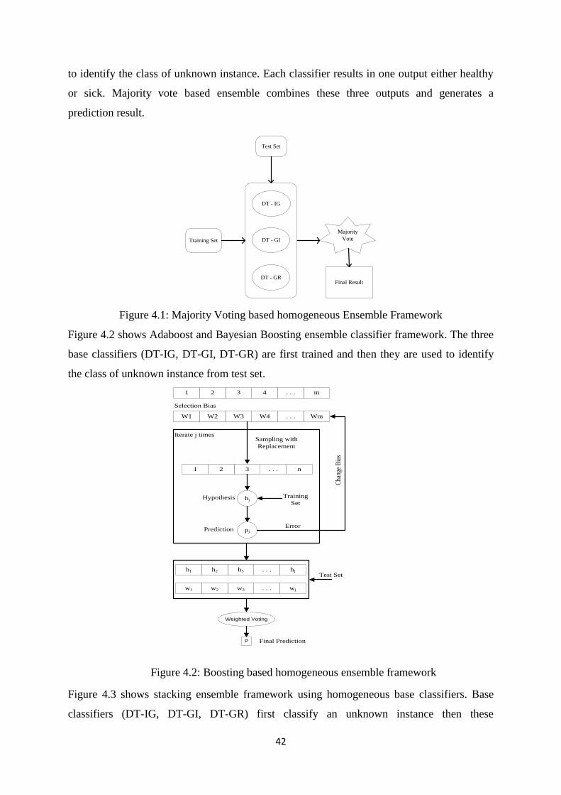
42
to identify the class of unknown instance. Each classifier results in one output either healthy
or sick. Majority vote based ensemble combines these three outputs and generates a
prediction result.
Training Set
Test Set
Majority
Vote
Final Result
DT - IG
DT - GR
DT - GI
Figure 4.1: Majority Voting based homogeneous Ensemble Framework
Figure 4.2 shows Adaboost and Bayesian Boosting ensemble classifier framework. The three
base classifiers (DT-IG, DT-GI, DT-GR) are first trained and then they are used to identify
the class of unknown instance from test set.
m. . .4321
Wm. . .W4W3W2W1
Selection Bias
n. . .321
Sampling with
Replacement
hjHypothesis Training
Set
pjPredictionError
Cha
nge
Bia
s
Iterate j times
hj. . .h3h2h1
wj. . .w3w2w1
Test Set
Weighted Voting
P Final Prediction
Figure 4.2: Boosting based homogeneous ensemble framework
Figure 4.3 shows stacking ensemble framework using homogeneous base classifiers. Base
classifiers (DT-IG, DT-GI, DT-GR) first classify an unknown instance then these
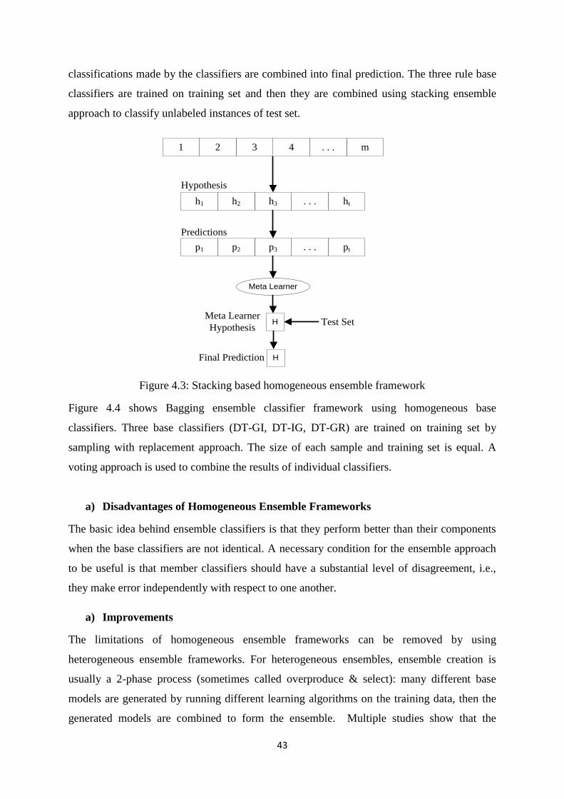
43
classifications made by the classifiers are combined into final prediction. The three rule base
classifiers are trained on training set and then they are combined using stacking ensemble
approach to classify unlabeled instances of test set.
m. . .4321
ht. . .h3h2h1
pt. . .p3p2p1
Meta Learner
HMeta Learner
Hypothesis
Hypothesis
Predictions
Test Set
HFinal Prediction
Figure 4.3: Stacking based homogeneous ensemble framework
Figure 4.4 shows Bagging ensemble classifier framework using homogeneous base
classifiers. Three base classifiers (DT-GI, DT-IG, DT-GR) are trained on training set by
sampling with replacement approach. The size of each sample and training set is equal. A
voting approach is used to combine the results of individual classifiers.
a) Disadvantages of Homogeneous Ensemble Frameworks
The basic idea behind ensemble classifiers is that they perform better than their components
when the base classifiers are not identical. A necessary condition for the ensemble approach
to be useful is that member classifiers should have a substantial level of disagreement, i.e.,
they make error independently with respect to one another.
a) Improvements
The limitations of homogeneous ensemble frameworks can be removed by using
heterogeneous ensemble frameworks. For heterogeneous ensembles, ensemble creation is
usually a 2-phase process (sometimes called overproduce & select): many different base
models are generated by running different learning algorithms on the training data, then the
generated models are combined to form the ensemble. Multiple studies show that the

44
strength of heterogeneous ensemble is related to the performance of the base classifiers and
the lack of correlation between them (model diversity). One way to decrease the correlations
between the classifiers while increasing or maintaining the overall performance of the
ensemble classifier is to include base classifiers derived from different learning algorithms
such as Decision Trees, Neural Networks, Perceptron and Support Vector Machine, etc.
m. . .4321
Training Set
n. . .321
Sampling with
Replacement
ht. . .h3h2h1
pt. . .p3p2p1
Voting
P Final Prediction
n. . .321
n. . .321
Bootstrap Sets
.
.
.
Set 1
Set 2
Set t
Figure 4.4: Bagging based homogeneous ensemble framework
4.3 Heterogeneous Ensemble Frameworks
Different variations of heterogeoeus ensemble frameworks that have been proposed in order
to improve disease prediction such as majority voting based ensemble, weighted voting based
ensemble and multi-criteria based weighted voting ensemble etc.
4.3.1 Majority Voting Ensemble Scheme
4.3.1.1 Three heterogeneous classifiers based Majority voting ensemble (MV3)
The first version of majority voting based ensemble framework that we have proposed is
based on three heterogeneous base classifiers for disease prediction. The three heterogeneous
classifiers are namely, Naïve Bayes (NB), Decision Tree based on Gini Index (DT-Gini) and
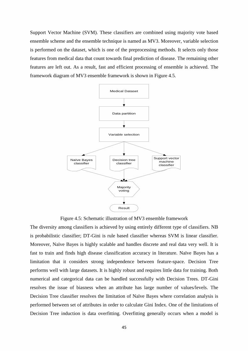
45
Support Vector Machine (SVM). These classifiers are combined using majority vote based
ensemble scheme and the ensemble technique is named as MV3. Moreover, variable selection
is performed on the dataset, which is one of the preprocessing methods. It selects only those
features from medical data that count towards final prediction of disease. The remaining other
features are left out. As a result, fast and efficient processing of ensemble is achieved. The
framework diagram of MV3 ensemble framework is shown in Figure 4.5.
Medical Dataset
Data partition
Variable selection
Naïve Bayes
classifier
Support vector
machine
classifier
Decision tree
classifier
Majority
voting
Result
Figure 4.5: Schematic illustration of MV3 ensemble framework
The diversity among classifiers is achieved by using entirely different type of classifiers. NB
is probabilistic classifier; DT-Gini is rule based classifier whereas SVM is linear classifier.
Moreover, Naïve Bayes is highly scalable and handles discrete and real data very well. It is
fast to train and finds high disease classification accuracy in literature. Naïve Bayes has a
limitation that it considers strong independence between feature-space. Decision Tree
performs well with large datasets. It is highly robust and requires little data for training. Both
numerical and categorical data can be handled successfully with Decision Trees. DT-Gini
resolves the issue of biasness when an attribute has large number of values/levels. The
Decision Tree classifier resolves the limitation of Naïve Bayes where correlation analysis is
performed between set of attributes in order to calculate Gini Index. One of the limitations of
Decision Tree induction is data overfitting. Overfitting generally occurs when a model is
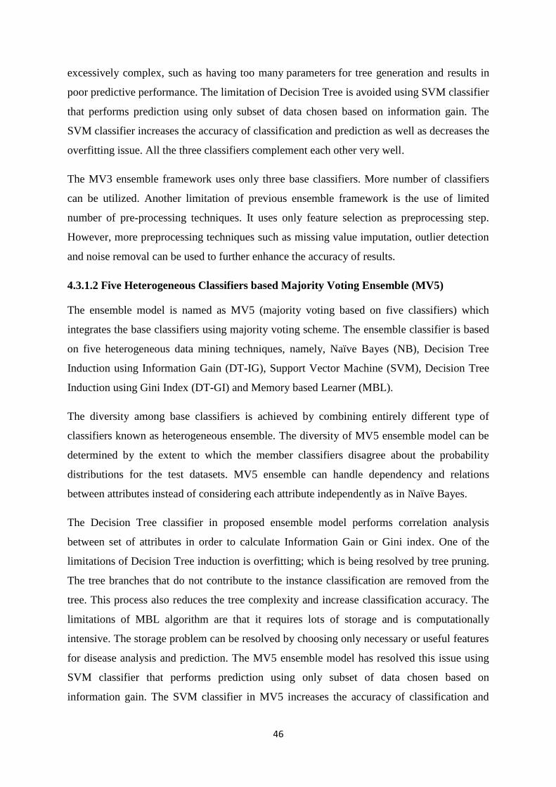
46
excessively complex, such as having too many parameters for tree generation and results in
poor predictive performance. The limitation of Decision Tree is avoided using SVM classifier
that performs prediction using only subset of data chosen based on information gain. The
SVM classifier increases the accuracy of classification and prediction as well as decreases the
overfitting issue. All the three classifiers complement each other very well.
The MV3 ensemble framework uses only three base classifiers. More number of classifiers
can be utilized. Another limitation of previous ensemble framework is the use of limited
number of pre-processing techniques. It uses only feature selection as preprocessing step.
However, more preprocessing techniques such as missing value imputation, outlier detection
and noise removal can be used to further enhance the accuracy of results.
4.3.1.2 Five Heterogeneous Classifiers based Majority Voting Ensemble (MV5)
The ensemble model is named as MV5 (majority voting based on five classifiers) which
integrates the base classifiers using majority voting scheme. The ensemble classifier is based
on five heterogeneous data mining techniques, namely, Naïve Bayes (NB), Decision Tree
Induction using Information Gain (DT-IG), Support Vector Machine (SVM), Decision Tree
Induction using Gini Index (DT-GI) and Memory based Learner (MBL).
The diversity among base classifiers is achieved by combining entirely different type of
classifiers known as heterogeneous ensemble. The diversity of MV5 ensemble model can be
determined by the extent to which the member classifiers disagree about the probability
distributions for the test datasets. MV5 ensemble can handle dependency and relations
between attributes instead of considering each attribute independently as in Naïve Bayes.
The Decision Tree classifier in proposed ensemble model performs correlation analysis
between set of attributes in order to calculate Information Gain or Gini index. One of the
limitations of Decision Tree induction is overfitting; which is being resolved by tree pruning.
The tree branches that do not contribute to the instance classification are removed from the
tree. This process also reduces the tree complexity and increase classification accuracy. The
limitations of MBL algorithm are that it requires lots of storage and is computationally
intensive. The storage problem can be resolved by choosing only necessary or useful features
for disease analysis and prediction. The MV5 ensemble model has resolved this issue using
SVM classifier that performs prediction using only subset of data chosen based on
information gain. The SVM classifier in MV5 increases the accuracy of classification and
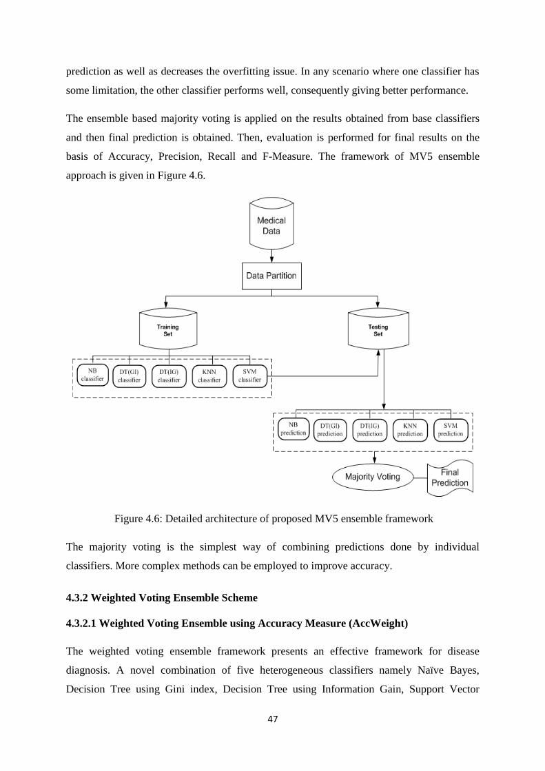
47
prediction as well as decreases the overfitting issue. In any scenario where one classifier has
some limitation, the other classifier performs well, consequently giving better performance.
The ensemble based majority voting is applied on the results obtained from base classifiers
and then final prediction is obtained. Then, evaluation is performed for final results on the
basis of Accuracy, Precision, Recall and F-Measure. The framework of MV5 ensemble
approach is given in Figure 4.6.
Figure 4.6: Detailed architecture of proposed MV5 ensemble framework
The majority voting is the simplest way of combining predictions done by individual
classifiers. More complex methods can be employed to improve accuracy.
4.3.2 Weighted Voting Ensemble Scheme
4.3.2.1 Weighted Voting Ensemble using Accuracy Measure (AccWeight)
The weighted voting ensemble framework presents an effective framework for disease
diagnosis. A novel combination of five heterogeneous classifiers namely Naïve Bayes,
Decision Tree using Gini index, Decision Tree using Information Gain, Support Vector

48
Machine and Memory based Learner are used to make an ensemble framework. Weighted
voting technique determines the final prediction where weights are assigned on the basis of
classification accuracy. The ensemble framework is named as AccWeight ensemble. The
classifier which has high accuracy will attain high weight and vice versa. The final prediction
will be done based on highest weighted vote.
Let the training data at level-0 is represented by D and it is randomly split into k disjoint
subsets of equal size such as D1,D2,……Dk . For each fold i=1,2,…k of the process, the
training set D/Di are used to train the base classifiers and then they are applied on the test set.
A meta instance is formed by the output generated from each base classifier along with the
true output class for each test instance. At meta level (level-1) weighted voting is applied on
the outputs generated from each base classifier. A weighted vote based classifier ensemble
method will then produce the final result. The weight is related to the classifier accuracy
value. Mathematically it is defined as:
∑
(4.1)
where Ei denotes the normalization factor. Each classifier outputs the weight for a class and a
class with highest resultant weight will be the proposed class for an instance determined by
ensemble. The classification of an unlabeled instance is performed according to the class that
has attained the highest weight of vote. Mathematically:
))),((*)((maxarg)( k
ikk cxygAAccxClass (4.2)
where yk represents the classification of kth
classifier and g(y,c) denotes the indicator function
defined as:
(4.3)
The working of ensemble classifier is shown in Figure 4.8 and explained as follows:
1. Four medical datasets are partitioned into training set and test set using 10 fold cross
validation.
2. Five individual classifiers are trained on training set. Accuracy of each classifier is
calculated. Following formula is used to calculate the accuracy of each classifier.
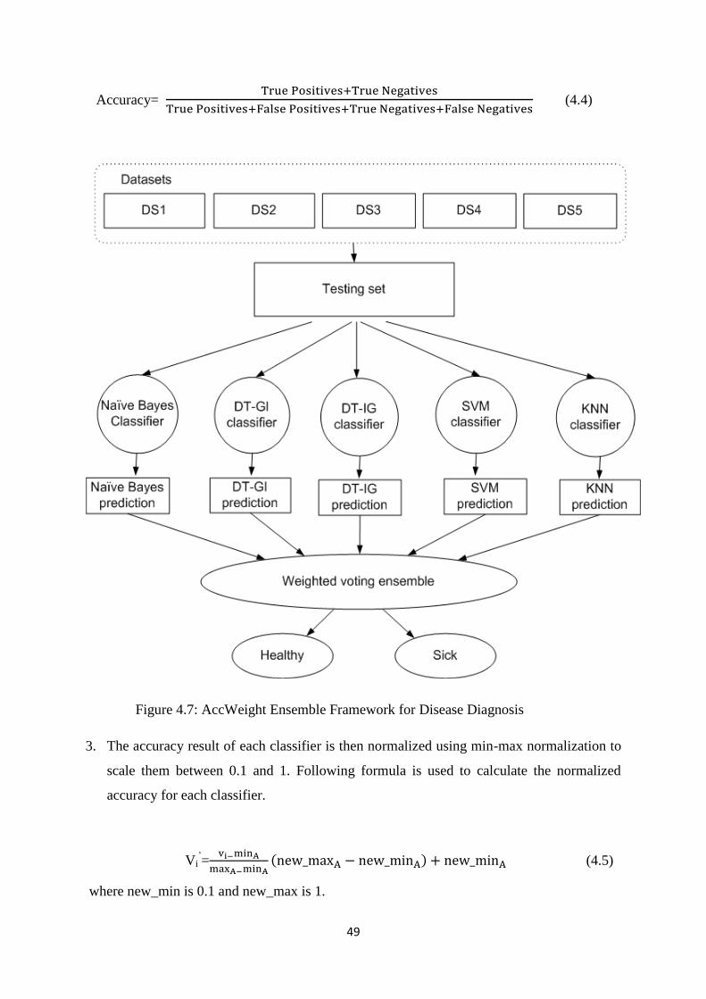
49
Accuracy=
(4.4)
Figure 4.7: AccWeight Ensemble Framework for Disease Diagnosis
3. The accuracy result of each classifier is then normalized using min-max normalization to
scale them between 0.1 and 1. Following formula is used to calculate the normalized
accuracy for each classifier.
Vi‘=
(4.5)
where new_min is 0.1 and new_max is 1.

50
4. The normalized accuracy value is directly proportional to the weight/vote of each
classifier.
5. Trained classifiers are then executed on test data. For a particular instance, each classifier
will predict an outcome class.
6. Ensemble classifier will then calculate the weight of each class. The class with higher
weight will be the output class for that test instance.
The AccWeight ensemble framework uses accuracy as weighing metric in weighted vote
based ensemble scheme. The biasness of accuracy results can be generated if we have biased
dataset in case of unbalanced classes. An unbiased metric is needed in order to assign the
weights to base classifiers instead of accuracy measure. Moreover, Sometimes a single
measure cannot capture the quality of a good ensemble reliably.
4.3.2.2 Weighted Voting Ensemble using F-Measure (FmWeight)
The enhanced version of weighted vote based ensemble framework performs weighted vote
based on F-Measure (Precision + Recall). The proposed ensemble model consists of five
heterogeneous classifiers: Naïve Bayes, Decision Tree based on Gini Index, Decision Tree
based on Information Gain, Instance based Learner and Support Vector Machines. Each
classifier is trained using training dataset and then F-Measure is calculated for each of them.
The classifier which has highest F-Measure will attain the highest weight and vice versa. The
final prediction is performed by combining the result of all classifiers and generating one
prediction result. The ensemble classifier is named as FmWeight ensemble classifier which
symbolizes weight calculation using F-Measure.
Both objective functions (Precision, Recall) achieve the two different classification qualities
and often there is inverse relationship between them where one is increased at the cost of
reducing the other. For example, the information retrieval system such as the search engine
increases the recall by retrieving the more files whereas the precision is decreased by
increasing the number of irrelevant files that are retrieved. Thus the motivation of FmWeight
ensemble classifier is to simultaneously optimize the two objectives.
The flow chart of FmWeight ensemble framework is shown in Figure 4.8. The F-Measure is
calculated for the training set using the precision and recall for all classifiers. The range of
these weights might be very high. The weights are then normalized in small scale by applying

51
min-max normalization to the f-measure values. The new_min is specified as 0.1 and
new_max is specified as 1. Following formula is used to calculate the min-max
normalization:
Vi‘=
(4.6)
where Vi is the value needed to be normalized, minA is minimum value for given dataset,
maxA is maximum value for given dataset and Vi‘ is normalized output value.
The precision represents the percentage of healthy samples labeled as healthy by the classifier
and is defined as follows:
Precision=
(4.7)
where true positives are correctly classified actual positives and false positives are actual
negatives that are incorrectly labeled as positives.
Recall represents the relevant instances that are retrieved by the classifier and is defined as
follows:
Recall=
(4.8)
where false negatives are incorrectly labeled data as negatives that are actual positives.
The F-Measure is the weighted average of Recall and Precision and is represented by:
(4.9)
The working of FmWeight ensemble classifier can be clearly understood by the following
example where class 0 present healthy patient record and class 1 presents unhealthy or sick
patient record.
1. Suppose that the classifier training is performed for training data and f-measure is
calculated. Following f-measure results are generated by each classifier:
NB=60%, DT-Gini= 70%, DT-info=80%, IBL=85%, SVM=90%
2. Now, votes are calculated using the formula given in equation (10) having
new_max=1, new_min=0.1, max=100, min=0. The resultant weights are as follows:
NB=0.6, DT-Gini=0.7, DT-Info=0.8, IBL=0.9, SVM= 0.9
3. Suppose, the classifiers have predicted the following classes for a test instance:
NB= Class 0, DT-Gini=Class 0, DT-Info= Class 1, IBL= Class 0, SVM= Class 1
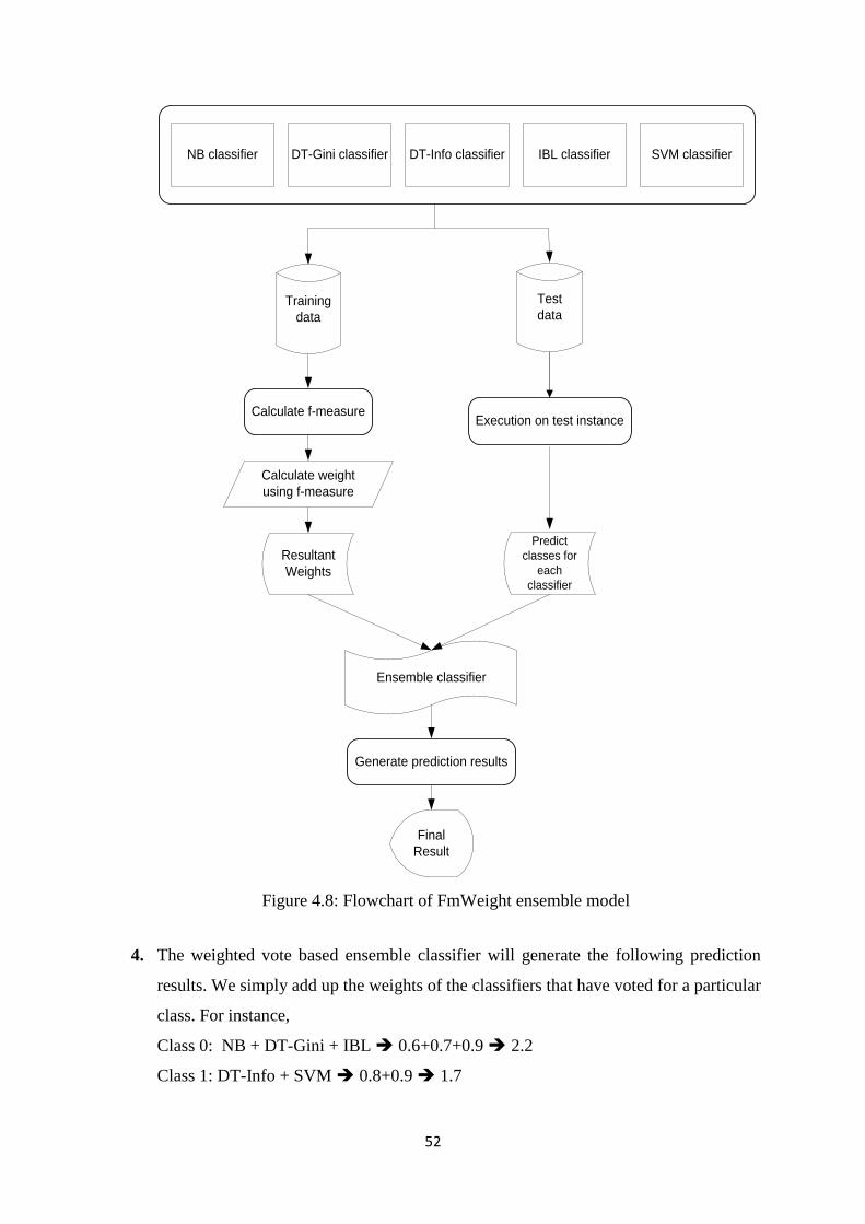
52
Training
data
NB classifier IBL classifier SVM classifierDT-Info classifierDT-Gini classifier
Calculate f-measure
Calculate weight
using f-measure
Resultant
Weights
Execution on test instance
Ensemble classifier
Generate prediction results
Final
Result
Test
data
Predict
classes for
each
classifier
Figure 4.8: Flowchart of FmWeight ensemble model
4. The weighted vote based ensemble classifier will generate the following prediction
results. We simply add up the weights of the classifiers that have voted for a particular
class. For instance,
Class 0: NB + DT-Gini + IBL 0.6+0.7+0.9 2.2
Class 1: DT-Info + SVM 0.8+0.9 1.7
53
5. Hence, according to weighted vote based ensemble classifier the class 0 has higher
value as compared to class 1. Therefore, the test instance will be classified as Class 0.
It was noticed that the weighted voting ensemble scheme generates high accuracy results as
compared to majority voting ensemble and individual classifiers. However by applying
bagging approach, it is possible to reduce the variance and leaves bias unchanged. Moreover,
it also helps to avoid overfitting, a problem that occurs during tree construction. A bagging
multi-objective optimization criterion along with weighted voting scheme is proposed to
reduce biasness, contradictions and to improve classification accuracy.
4.3.2.3 Bagging Approach with Multi-objective Weighted voting Ensemble Scheme
(BagMoov)
The enhancements are made in bagging approach with multi-objective weighted voting
scheme for prediction of disease. The multi-objective criteria are used to reduce the effect of
biasness and precision and recall are used for this purpose. Moreover, we argue that each
classifier in the bagging approach should not have the same weight as each classifier has a
different individual performance level. Therefore, we propose to use multi-objective
optimized weighting scheme instead of simple voting. The enhanced version of ensemble
framework is termed as BagMoov (Bagging approach with multi-objective optimized
weighted voting) ensemble framework. The ensemble model is composed of five
heterogeneous classifiers: Naïve Bayes, Linear Regression, Linear Discriminant Analysis,
Instance based Learner and Support Vector Machine.
The BagMoov ensemble framework utilizes diverse set of base classifiers that differ in their
decisions. The diversity among classifiers is achieved by entirely different type of classifiers
such as Naïve Bayes is probability based classifier which has high classification and
prediction accuracy. Linear regression is linear classifier which has the advantages of
simplicity, interpretability, scientific acceptance and widespread availability. Linear
discriminant analysis is a common tool for classification which has quadratic decision surface
and requires no parameters to tune the algorithm. It is inherently multiclass and proven to
work well in practice. Instance based learner classifier is distance based classifier which does
not build model explicitly. It may simply store a new instance or throw an old instance away.
Instance based learner avoids the risk of overfitting to noise in the training set. Support
Vector Machines are used for classification, regression and outlier detection. It is effective in

54
high dimensional space and use different kernel functions for making decisions. Hence, each
classifier in BagMoov ensemble framework has diverse set of qualities that complement each
other to make an accurate ensemble framework for disease classification and prediction. The
BagMoov ensemble framework is shown in Figure 4.9.
Figure 4.9: BagMoov ensemble algorithm
At first stage, original training set for each dataset is divided into multiple bootstrap sets with
replacement. In order to create bootstrap samples from training set of size m, t multinomial
trails are performed, where one of the m examples is drawn for each trial. The probability of
each example to be drawn in each trial is 1/m. The proposed ensemble algorithm chooses a
sample r from 1 to m and the rth
training example is added to bootstrap training set S.
Moreover, it is possible that some of the training examples will not be selected in bootstrap
training sets whereas others may be chosen one time or more. At second stage, classifiers‘
training is performed using bootstrap training sets generated during the first stage.
We argue that each classifier in the bagging approach should not have the same weight as
each classifier has a different individual performance level. Therefore, we propose to use
multi-objective optimized weighting scheme instead of simple voting. The BagMoov

55
ensemble will return a function h(d) that classifies new samples into class y having the
highest weight from the base models h1,h2,h3,……,ht. t bootstrap training sets are created
which have some differences with each other. The ensemble model will perform better than
individual classifier if the difference among bootstrap training sets induces a noticeable
difference among M individual classifiers, generating reasonably good performance by each
of them. It is also proposed that a bagged ensemble approach outperforms each base classifier
if the base classifiers are trained using sample sets where differences in sample training sets
induce a significant difference in the base classifiers.
The BagMoov ensemble classifier is based on the principle of multi-objective where we try to
optimize multiple goals simultaneously. Formally, it can be stated as: Find the number of
vectors Vk where Vk={v1,v2,v3,……vn} for each classifier Ck and Ck={C1,C2,C3…Cn} such
that simultaneously optimize the N objective criteria, while satisfying the constraints, if any.
The multi-objective optimization focuses on the maximization problem which states that a
solution vi will always dominate a solution vj if for all K 1,2,3…..N, fk(vi) > fk(vj) where fk is
an objective function. The maximization problem stands true for each objective function used
for the BagMoov classifier ensemble technique.
The choice of objective functions should be as much contradictory as possible in order to
achieve high performance of weighted voting for ensemble classifier. We have used precision
and recall as two objective functions as previously discussed. The recall tries to increase the
number of healthy samples while precision tries to increase the number of correct healthy
samples as much as possible. The f-measure is then calculated for the training set using the
precision and recall for each classifier. F-measure results in a value (weight) that has the
highest precision and recall combination. The weights are then normalized by applying min-
max normalization as discussed earlier.
The working of ensemble classifier can be easily understood by the following example,
where class 0 present healthy patient record and class 1 presents unhealthy or sick patient
record.
1. Suppose that the classifier training is performed for training data and f-measure is
calculated. Following f-measure results are generated for each classifier:
NB=60%, LR= 70%, LDA=80%, IBL=85%, SVM=90%
2. Now, votes are calculated using the formula given in equation (10) having
new_max=1.0, new_min=0.1, max=100, min=0. The resultant weights are as follows:
NB=0.6, LR=0.7, LDA=0.8, IBL=0.9, SVM= 0.9
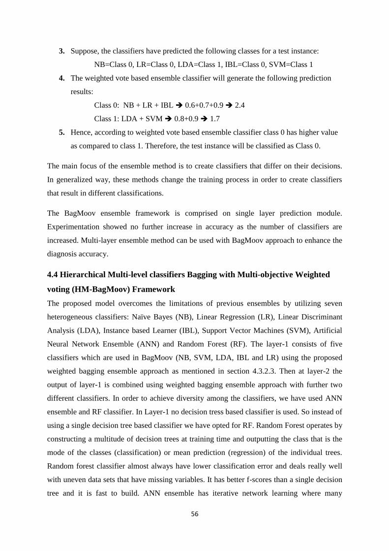
56
3. Suppose, the classifiers have predicted the following classes for a test instance:
NB=Class 0, LR=Class 0, LDA=Class 1, IBL=Class 0, SVM=Class 1
4. The weighted vote based ensemble classifier will generate the following prediction
results:
Class 0: NB + LR + IBL 0.6+0.7+0.9 2.4
Class 1: LDA + SVM 0.8+0.9 1.7
5. Hence, according to weighted vote based ensemble classifier class 0 has higher value
as compared to class 1. Therefore, the test instance will be classified as Class 0.
The main focus of the ensemble method is to create classifiers that differ on their decisions.
In generalized way, these methods change the training process in order to create classifiers
that result in different classifications.
The BagMoov ensemble framework is comprised on single layer prediction module.
Experimentation showed no further increase in accuracy as the number of classifiers are
increased. Multi-layer ensemble method can be used with BagMoov approach to enhance the
diagnosis accuracy.
4.4 Hierarchical Multi-level classifiers Bagging with Multi-objective Weighted
voting (HM-BagMoov) Framework
The proposed model overcomes the limitations of previous ensembles by utilizing seven
heterogeneous classifiers: Naïve Bayes (NB), Linear Regression (LR), Linear Discriminant
Analysis (LDA), Instance based Learner (IBL), Support Vector Machines (SVM), Artificial
Neural Network Ensemble (ANN) and Random Forest (RF). The layer-1 consists of five
classifiers which are used in BagMoov (NB, SVM, LDA, IBL and LR) using the proposed
weighted bagging ensemble approach as mentioned in section 4.3.2.3. Then at layer-2 the
output of layer-1 is combined using weighted bagging ensemble approach with further two
different classifiers. In order to achieve diversity among the classifiers, we have used ANN
ensemble and RF classifier. In Layer-1 no decision tress based classifier is used. So instead of
using a single decision tree based classifier we have opted for RF. Random Forest operates by
constructing a multitude of decision trees at training time and outputting the class that is the
mode of the classes (classification) or mean prediction (regression) of the individual trees.
Random forest classifier almost always have lower classification error and deals really well
with uneven data sets that have missing variables. It has better f-scores than a single decision
tree and it is fast to build. ANN ensemble has iterative network learning where many

57
problems are solved without finding and describing method of such problem solving, without
building algorithms, without developing programs, even without any case of knowledge
about the nature of solved problem. Neural network classifier with back propagation learning
capability has very low prediction error. The most important advantage of using ANN
ensemble is the ability to implicitly detect complex nonlinear relationships among variables.
Such a characteristic makes the ANNs suitable for prediction and pattern recognition
applications. The final prediction is obtained at layer-3. For each classifier, the weight is
calculated based on F-Measure of the training dataset. The final output of the ensemble
classifier is labeled with the class that has the highest weighted vote In order to further
improve the accuracy, pre-processing module has also been added to the framework. Pre-
processing steps involve: missing value imputation, outlier detection, feature selection and
noise removal.
4.4.1 Pre-processing Module
The pre-processing phase involves multiple steps that are applied on each dataset
sequentially. It includes feature selection, missing value imputation, noise removal and
outlier detection. The flow diagram of data preprocessing is shown in Figure 4.10.
4.4.1.1 Feature selection
This process involves feature reduction by selecting only those attributes which contribute
towards final prediction of disease. The rejected features will not be used for subsequent
modules and analysis. There are multiple steps involved in the process of feature selection
and identification. The generation and selection procedures are two of the most important
steps. The generation procedure involves generating features subset whereas selection
procedure will evaluate these features on the basis of different criteria. The generation
procedure can result in an empty set, subset based on randomly selected attributes or a set
based on all attributes. Forward selection is used in case of empty set which iteratively adds
the attributes in feature set whereas backward elimination is used in case of all attributes,
which iteratively eliminates the irrelevant attributes from feature set. The relevancy of an
attribute is measured by wrapper approaches. The main focus of a wrapper approach is
classification accuracy. The estimation accuracy of each feature set is calculated that is a
candidate for adding or removing from the dataset. We have used cross validation for
accuracy estimation of each feature set of the training set. The feature selection process
continues until pre-specified number of features is achieved or some threshold criteria are
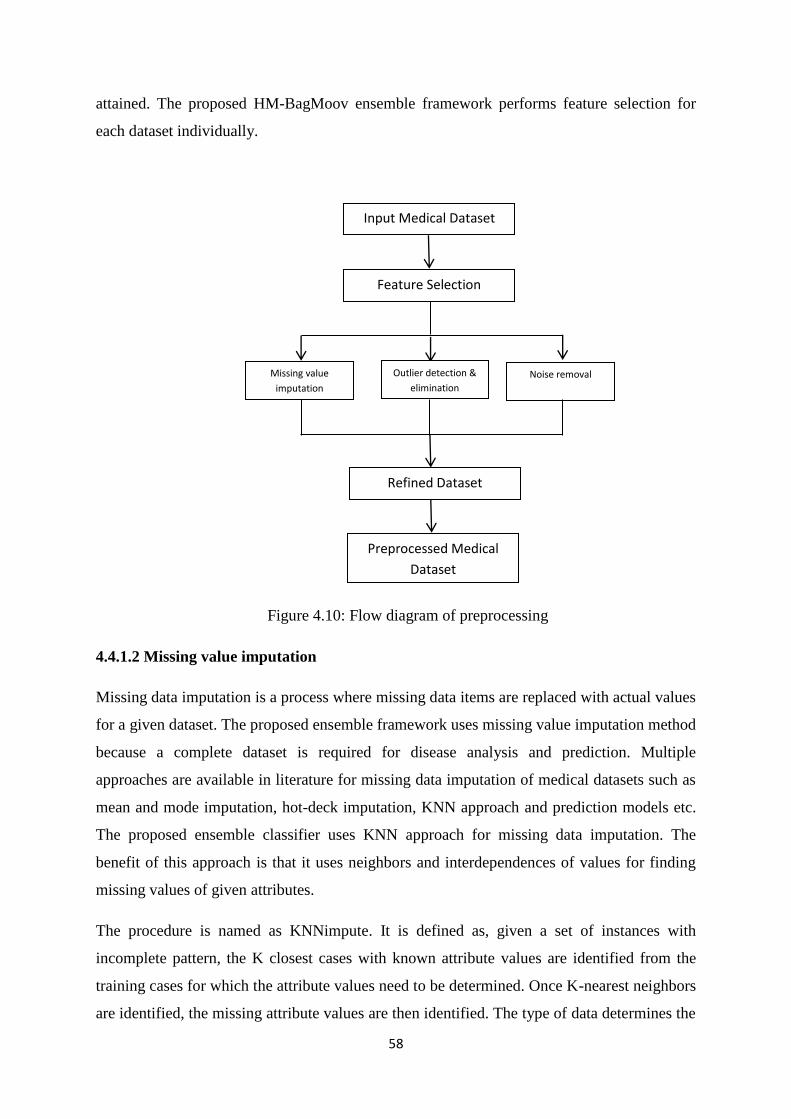
58
attained. The proposed HM-BagMoov ensemble framework performs feature selection for
each dataset individually.
Figure 4.10: Flow diagram of preprocessing
4.4.1.2 Missing value imputation
Missing data imputation is a process where missing data items are replaced with actual values
for a given dataset. The proposed ensemble framework uses missing value imputation method
because a complete dataset is required for disease analysis and prediction. Multiple
approaches are available in literature for missing data imputation of medical datasets such as
mean and mode imputation, hot-deck imputation, KNN approach and prediction models etc.
The proposed ensemble classifier uses KNN approach for missing data imputation. The
benefit of this approach is that it uses neighbors and interdependences of values for finding
missing values of given attributes.
The procedure is named as KNNimpute. It is defined as, given a set of instances with
incomplete pattern, the K closest cases with known attribute values are identified from the
training cases for which the attribute values need to be determined. Once K-nearest neighbors
are identified, the missing attribute values are then identified. The type of data determines the
Input Medical Dataset
Feature Selection
Missing value
imputation
Outlier detection &
elimination
Noise removal
Refined Dataset
Preprocessed Medical
Dataset

59
replacement value. For example, qualitative data value is determined using mode whereas the
mean value is used for continuous data. An appropriate distance measure is used to determine
the K-nearest neighbors and then to impute the missing value. The proposed missing data
imputation technique uses heterogeneous Euclidean-overlap metric (HEOM) for distance
measure between two variables. The benefit of using heterogeneous distance function is that
it can calculate different distance measures for different types of attributes. For instance, xa
and xb are two variables and distance between them is denoted by d(xa,xb). Following formula
is used to calculate the distance:
d(xa,xb)= 2bjaj
n
1j
j )x,(xd (4.10)
where distance is determined for jth attribute. Moreover:
d ),( bjaj xx =)15.4(
),(
),(
0)1)(1(,1
0
vequantitatiisxxxd
equalitativisxxxd
mm
jbjajN
jbjaj
bjaj
If either of input value is known then a distance value of 1 (i.e. maximal distance) is returned
for unknown data. d0 is an overlap distance function which assigns a value of 0 if qualitative
features are same other d=1. For example:
),(0 bjaj xxd =
bjaj
bjaj
xx
xx
1
0
(4.12)
dN is named as range normalized distance function which is defined as:
),( bjajN xxd =
(4.13)
Where maximum and minimum values of N training instances are represented by max (xj)
and min (xj) for jth continuous attribute.
Consider jth attribute is missing for an instance x i.e. mj=1. The distance of x from all
training instances is calculated and K-nearest neighbors are identified. The given notation:
Vx= (4.14)
)min()max(
||
jj
bjaj
xx
xx
K
kkV1
(4.11)

60
Where k-nearest neighbors of x are arranged in increasing distance order. For instance, v1 is
the closest neighbor of x. Once K-nearest neighbors are identified, the unknown value is
determined by an estimate from jth feature values of Vx.
If the jth feature value is continuous value, then missing value is replaced by mean value of
its K nearest neighbors. The weighted measure can be used where greater weight is given to
closest neighbor. Therefore:
Xj=
(4.15)
Where wk represents the weight of kth nearest neighbor.
If the jth input feature is qualitative value then the missing value is imputed by determining
the category of value using Vx. The mode of is imputed where same importance is
given to all neighbors. A weighted method assigns a weight to each Vk and closer
neighbors are assigned greater weight. The grouping is performed using discrete value in the
jth input feature. The distance weighted method for KNN classifier where is calculated by:
(x)=
(4.16)
Where k (x)= 1 when all distances are equal. For imputation, consider the jth feature is
qualitative having S possible discrete values. The imputed value is given by
S= argmax { } (4.17)
Where s is the possible category that is determined as imputed value.
The missing value imputation method can be defined by flowchart given in Figure 4.11.
4.4.1.3 Outlier detection and elimination
We have used Grubb‘s test for outlier values that may exist in medical datasets. There are
several reasons for outliers in disease data such as abnormal condition of patient or
equipment malfunction or recording error. Grubb‘s test is also called ESD (Extreme
Studentized Deviate) method. This method is beneficial as it considers complete dataset
values for outlier detection and elimination. Moreover background knowledge and
k
k
kjk vwKW 1
1
K
kkV1
k
k
k),1(),(
),(),(
xVdxVd
xVdxVd
k
kk
sx

61
interdependencies of variables are also taken into account by calculating mean and standard
deviation. This test is performed as long as all outliers will be detected. It is a two-step
Figure 4.11: Proposed missing data imputation method
process. First step is to calculate how far the outliers are from others. The ratio G is
calculated in second step that is the difference between dataset value and mean divided by
standard deviation. Following formula is used to determine outliers using Grubb‘s test.
G=
Medical Dataset
No missing
attribute
value
Records with
missing
values
Train the classifier with data having no missing
value and output is the attribute which value
needs to predict
Impute the predicted value in missing field
Instances
with imputed
value by KNN
classifier
Repeat for all the
attributes
Combined
data
)22.4(||max .......1
xxini (4.18)
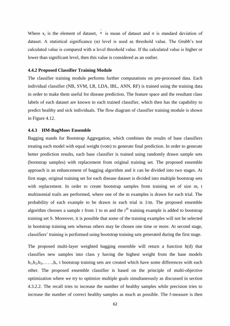
62
Where xi is the element of dataset, is mean of dataset and σ is standard deviation of
dataset. A statistical significance (α) level is used as threshold value. The Grubb‘s test
calculated value is compared with α level threshold value. If the calculated value is higher or
lower than significant level, then this value is considered as an outlier.
4.4.2 Proposed Classifier Training Module
The classifier training module performs further computations on pre-processed data. Each
individual classifier (NB, SVM, LR, LDA, IBL, ANN, RF) is trained using the training data
in order to make them useful for disease prediction. The feature space and the resultant class
labels of each dataset are known to each trained classifier, which then has the capability to
predict healthy and sick individuals. The flow diagram of classifier training module is shown
in Figure 4.12.
4.4.3 HM-BagMoov Ensemble
Bagging stands for Bootstrap Aggregation, which combines the results of base classifiers
treating each model with equal weight (vote) to generate final prediction. In order to generate
better prediction results, each base classifier is trained using randomly drawn sample sets
(bootstrap samples) with replacement from original training set. The proposed ensemble
approach is an enhancement of bagging algorithm and it can be divided into two stages. At
first stage, original training set for each disease dataset is divided into multiple bootstrap sets
with replacement. In order to create bootstrap samples from training set of size m, t
multinomial trails are performed, where one of the m examples is drawn for each trial. The
probability of each example to be drawn in each trial is 1/m. The proposed ensemble
algorithm chooses a sample r from 1 to m and the rth
training example is added to bootstrap
training set S. Moreover, it is possible that some of the training examples will not be selected
in bootstrap training sets whereas others may be chosen one time or more. At second stage,
classifiers‘ training is performed using bootstrap training sets generated during the first stage.
The proposed multi-layer weighted bagging ensemble will return a function h(d) that
classifies new samples into class y having the highest weight from the base models
h1,h2,h3,……,ht. t bootstrap training sets are created which have some differences with each
other. The proposed ensemble classifier is based on the principle of multi-objective
optimization where we try to optimize multiple goals simultaneously as discussed in section
4.3.2.2. The recall tries to increase the number of healthy samples while precision tries to
increase the number of correct healthy samples as much as possible. The f-measure is then
x
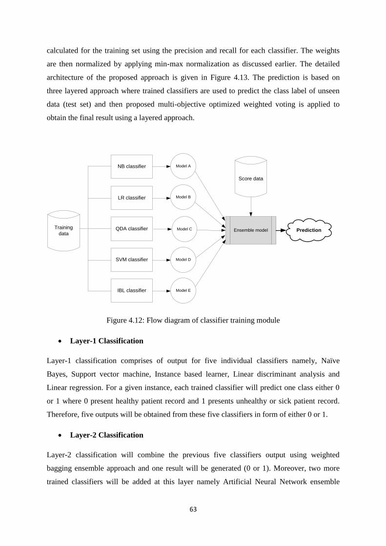
63
calculated for the training set using the precision and recall for each classifier. The weights
are then normalized by applying min-max normalization as discussed earlier. The detailed
architecture of the proposed approach is given in Figure 4.13. The prediction is based on
three layered approach where trained classifiers are used to predict the class label of unseen
data (test set) and then proposed multi-objective optimized weighted voting is applied to
obtain the final result using a layered approach.
Figure 4.12: Flow diagram of classifier training module
Layer-1 Classification
Layer-1 classification comprises of output for five individual classifiers namely, Naïve
Bayes, Support vector machine, Instance based learner, Linear discriminant analysis and
Linear regression. For a given instance, each trained classifier will predict one class either 0
or 1 where 0 present healthy patient record and 1 presents unhealthy or sick patient record.
Therefore, five outputs will be obtained from these five classifiers in form of either 0 or 1.
Layer-2 Classification
Layer-2 classification will combine the previous five classifiers output using weighted
bagging ensemble approach and one result will be generated (0 or 1). Moreover, two more
trained classifiers will be added at this layer namely Artificial Neural Network ensemble
Training
data
NB classifier
IBL classifier
SVM classifier
QDA classifier
LR classifier
Model A
Model B
Model C
Model D
Model E
Ensemble model
Score data
Prediction
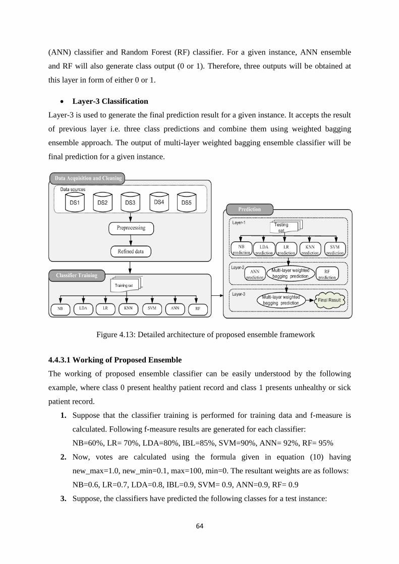
64
(ANN) classifier and Random Forest (RF) classifier. For a given instance, ANN ensemble
and RF will also generate class output (0 or 1). Therefore, three outputs will be obtained at
this layer in form of either 0 or 1.
Layer-3 Classification
Layer-3 is used to generate the final prediction result for a given instance. It accepts the result
of previous layer i.e. three class predictions and combine them using weighted bagging
ensemble approach. The output of multi-layer weighted bagging ensemble classifier will be
final prediction for a given instance.
Figure 4.13: Detailed architecture of proposed ensemble framework
4.4.3.1 Working of Proposed Ensemble
The working of proposed ensemble classifier can be easily understood by the following
example, where class 0 present healthy patient record and class 1 presents unhealthy or sick
patient record.
1. Suppose that the classifier training is performed for training data and f-measure is
calculated. Following f-measure results are generated for each classifier:
NB=60%, LR= 70%, LDA=80%, IBL=85%, SVM=90%, ANN= 92%, RF= 95%
2. Now, votes are calculated using the formula given in equation (10) having
new_max=1.0, new_min=0.1, max=100, min=0. The resultant weights are as follows:
NB=0.6, LR=0.7, LDA=0.8, IBL=0.9, SVM= 0.9, ANN=0.9, RF= 0.9
3. Suppose, the classifiers have predicted the following classes for a test instance:

65
NB=Class 0, LR=Class 0, LDA=Class 1, IBL=Class 0, SVM=Class 1, ANN=Class 0,
RF=Class 1
4. The weighted vote based ensemble classifier will generate the following prediction
results for layer-1:
Class 0: NB + LR + IBL 0.6+0.7+0.9 2.4
Class 1: LDA + SVM 0.8+0.9 1.7
5. Hence, according to weighted vote based ensemble classifier class 0 has higher value
as compared to class 1. Therefore, class 0 will return as output to layer-2.
6. Now, the weighted vote based ensemble classifier will generate the following
prediction results for layer-2:
Class 0: Multi-Layer Weighted Bagging + ANN ensemble (2.4/3)+0.91.7
Class 1: RF 0.9
7. Hence, according to weighted vote based ensemble classifier class 0 has higher value
as compared to class 1. Therefore, class 0 will return as output to layer-3 and will be
the final prediction by proposed ensemble technique.
For the rest of the thesis HM-BagMoov and HM-BagMoov framework will be used
interchangeably.
4.5 Summary
Ensemble of classifiers has been proved to be very effective way to improve classification
accuracy because uncorrelated errors made by a single classifier can be removed by voting.
We have proposed seven different versions of ensemble frameworks for disease diagnosis.
These comprised of multiple homogeneous and heterogeneous data mining techniques. The
first and most basic ensemble framework is comprised of homogeneous data mining
techniques. Then, heterogeneous data mining ensemble frameworks have been introduced to
overcome the limitations of previous ensemble frameworks. Each heterogeneous ensemble
framework is refined in forthcoming version in order to overcome the limitations of previous
version. Finally, we have proposed a multi-layer multi-classifier ensemble framework for
disease diagnosis with high accuracy.
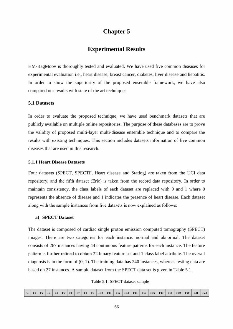
66
Chapter 5
Experimental Results
HM-BagMoov is thoroughly tested and evaluated. We have used five common diseases for
experimental evaluation i.e., heart disease, breast cancer, diabetes, liver disease and hepatitis.
In order to show the superiority of the proposed ensemble framework, we have also
compared our results with state of the art techniques.
5.1 Datasets
In order to evaluate the proposed technique, we have used benchmark datasets that are
publicly available on multiple online repositories. The purpose of these databases are to prove
the validity of proposed multi-layer multi-disease ensemble technique and to compare the
results with existing techniques. This section includes datasets information of five common
diseases that are used in this research.
5.1.1 Heart Disease Datasets
Four datasets (SPECT, SPECTF, Heart disease and Statlog) are taken from the UCI data
repository, and the fifth dataset (Eric) is taken from the record data repository. In order to
maintain consistency, the class labels of each dataset are replaced with 0 and 1 where 0
represents the absence of disease and 1 indicates the presence of heart disease. Each dataset
along with the sample instances from five datasets is now explained as follows:
a) SPECT Dataset
The dataset is composed of cardiac single proton emission computed tomography (SPECT)
images. There are two categories for each instance: normal and abnormal. The dataset
consists of 267 instances having 44 continuous feature patterns for each instance. The feature
pattern is further refined to obtain 22 binary feature set and 1 class label attribute. The overall
diagnosis is in the form of (0, 1). The training data has 240 instances, whereas testing data are
based on 27 instances. A sample dataset from the SPECT data set is given in Table 5.1.
Table 5.1: SPECT dataset sample
G F1 F2 F3 F4 F5 F6 F7 F8 F9 F10 F11 F12 F13 F14 F15 F16 F17 F18 F19 F20 F21 F22
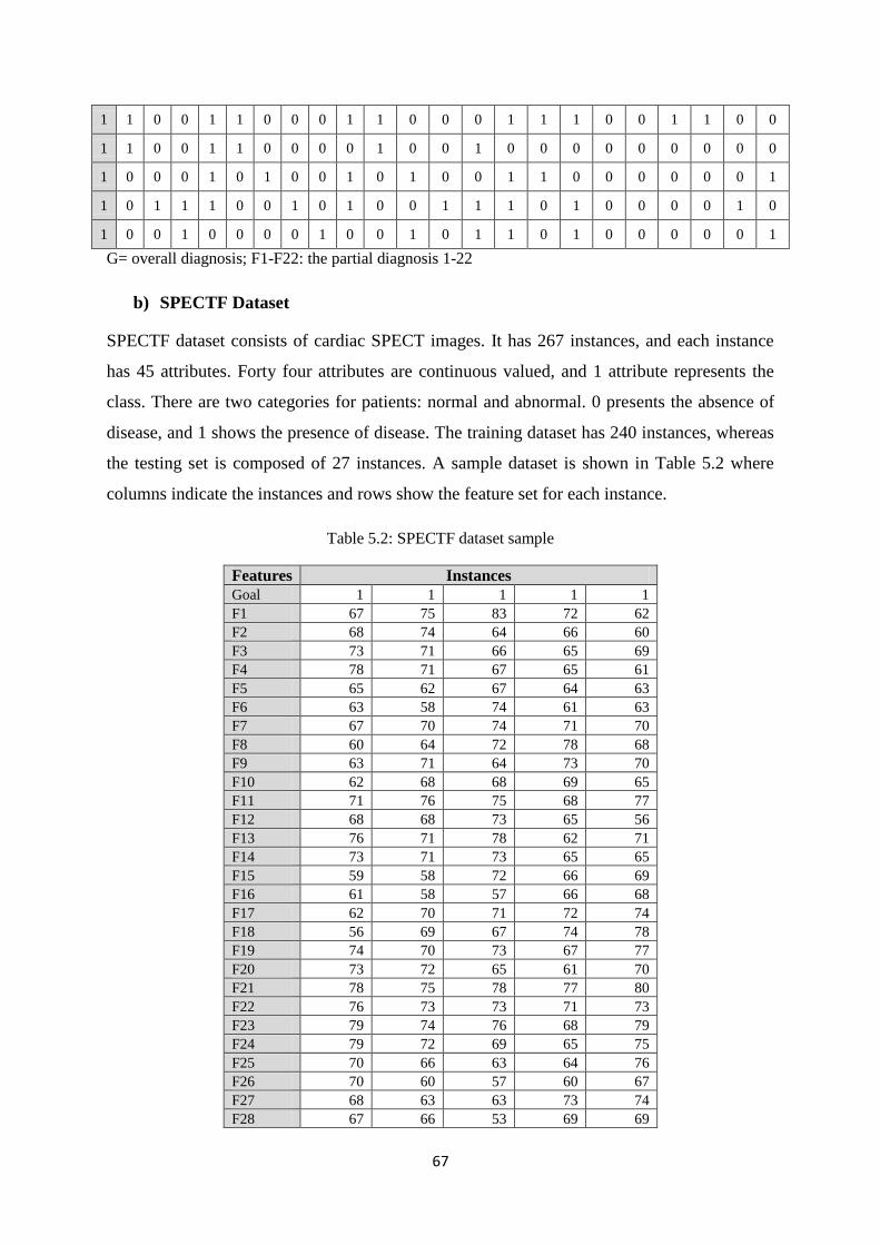
67
1 1 0 0 1 1 0 0 0 1 1 0 0 0 1 1 1 0 0 1 1 0 0
1 1 0 0 1 1 0 0 0 0 1 0 0 1 0 0 0 0 0 0 0 0 0
1 0 0 0 1 0 1 0 0 1 0 1 0 0 1 1 0 0 0 0 0 0 1
1 0 1 1 1 0 0 1 0 1 0 0 1 1 1 0 1 0 0 0 0 1 0
1 0 0 1 0 0 0 0 1 0 0 1 0 1 1 0 1 0 0 0 0 0 1
G= overall diagnosis; F1-F22: the partial diagnosis 1-22
b) SPECTF Dataset
SPECTF dataset consists of cardiac SPECT images. It has 267 instances, and each instance
has 45 attributes. Forty four attributes are continuous valued, and 1 attribute represents the
class. There are two categories for patients: normal and abnormal. 0 presents the absence of
disease, and 1 shows the presence of disease. The training dataset has 240 instances, whereas
the testing set is composed of 27 instances. A sample dataset is shown in Table 5.2 where
columns indicate the instances and rows show the feature set for each instance.
Table 5.2: SPECTF dataset sample
Features Instances
Goal 1 1 1 1 1
F1 67 75 83 72 62
F2 68 74 64 66 60
F3 73 71 66 65 69
F4 78 71 67 65 61
F5 65 62 67 64 63
F6 63 58 74 61 63
F7 67 70 74 71 70
F8 60 64 72 78 68
F9 63 71 64 73 70
F10 62 68 68 69 65
F11 71 76 75 68 77
F12 68 68 73 65 56
F13 76 71 78 62 71
F14 73 71 73 65 65
F15 59 58 72 66 69
F16 61 58 57 66 68
F17 62 70 71 72 74
F18 56 69 67 74 78
F19 74 70 73 67 77
F20 73 72 65 61 70
F21 78 75 78 77 80
F22 76 73 73 71 73
F23 79 74 76 68 79
F24 79 72 69 65 75
F25 70 66 63 64 76
F26 70 60 57 60 67
F27 68 63 63 73 74
F28 67 66 53 69 69
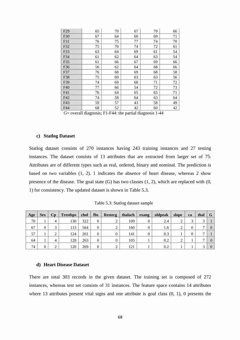
68
F29 65 70 67 70 66
F30 67 64 60 69 71
F31 76 75 77 74 70
F32 75 70 74 72 61
F33 63 64 69 61 54
F34 61 62 64 63 54
F35 61 66 67 69 66
F36 56 62 64 68 66
F37 76 68 69 68 58
F38 75 69 63 63 56
F39 74 69 68 71 72
F40 77 66 54 72 73
F41 76 64 65 65 71
F42 74 58 64 63 64
F43 59 57 43 58 49
F44 68 52 42 60 42
G= overall diagnosis; F1-F44: the partial diagnosis 1-44
c) Statlog Dataset
Statlog dataset consists of 270 instances having 243 training instances and 27 testing
instances. The dataset consists of 13 attributes that are extracted from larger set of 75.
Attributes are of different types such as real, ordered, binary and nominal. The prediction is
based on two variables (1, 2). 1 indicates the absence of heart disease, whereas 2 show
presence of the disease. The goal state (G) has two classes (1, 2), which are replaced with (0,
1) for consistency. The updated dataset is shown in Table 5.3.
Table 5.3: Statlog dataset sample
Age Sex Cp Trestbps chol fbs Restecg thalach exang oldpeak slope ca thal G
70 1 4 130 322 0 2 109 0 2.4 2 3 3 1
67 0 3 115 564 0 2 160 0 1.6 2 0 7 0
57 1 2 124 261 0 0 141 0 0.3 1 0 7 1
64 1 4 128 263 0 0 105 1 0.2 2 1 7 0
74 0 2 120 269 0 2 121 1 0.2 1 1 3 0
d) Heart Disease Dataset
There are total 303 records in the given dataset. The training set is composed of 272
instances, whereas test set consists of 31 instances. The feature space contains 14 attributes
where 13 attributes present vital signs and one attribute is goal class (0, 1), 0 presents the
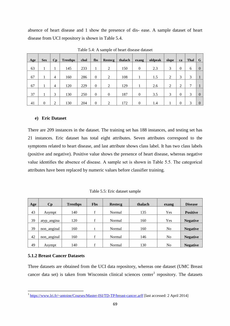
69
absence of heart disease and 1 show the presence of dis- ease. A sample dataset of heart
disease from UCI repository is shown in Table 5.4.
Table 5.4: A sample of heart disease dataset
e) Eric Dataset
There are 209 instances in the dataset. The training set has 188 instances, and testing set has
21 instances. Eric dataset has total eight attributes. Seven attributes correspond to the
symptoms related to heart disease, and last attribute shows class label. It has two class labels
(positive and negative). Positive value shows the presence of heart disease, whereas negative
value identifies the absence of disease. A sample set is shown in Table 5.5. The categorical
attributes have been replaced by numeric values before classifier training.
Table 5.5: Eric dataset sample
Age Cp Trestbps Fbs Restecg thalach exang Disease
43 Asympt 140 f Normal 135 Yes Positive
39 atyp_angina 120 f Normal 160 Yes Negative
39 non_anginal 160 t Normal 160 No Negative
42 non_anginal 160 f Normal 146 No Negative
49 Asympt 140 f Normal 130 No Negative
5.1.2 Breast Cancer Datasets
Three datasets are obtained from the UCI data repository, whereas one dataset (UMC Breast
cancer data set) is taken from Wisconsin clinical sciences center1 repository. The datasets
1 https://www.lri.fr/~antoine/Courses/Master-ISI/TD-TP/breast-cancer.arff [last accessed: 2 April 2014]
Age Sex Cp Trestbps chol fbs Restecg thalach exang oldpeak slope ca Thal G
63 1 1 145 233 1 2 150 0 2.3 3 0 6 0
67 1 4 160 286 0 2 108 1 1.5 2 3 3 1
67 1 4 120 229 0 2 129 1 2.6 2 2 7 1
37 1 3 130 250 0 0 187 0 3.5 3 0 3 0
41 0 2 130 204 0 2 172 0 1.4 1 0 3 0
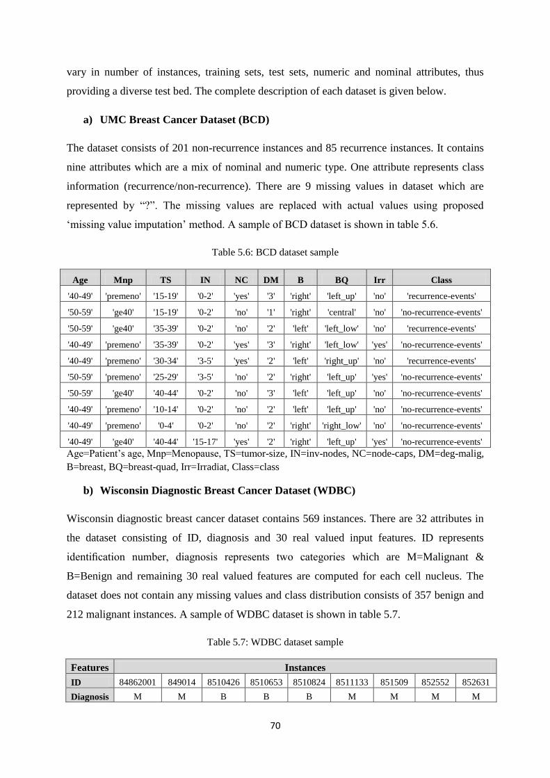
70
vary in number of instances, training sets, test sets, numeric and nominal attributes, thus
providing a diverse test bed. The complete description of each dataset is given below.
a) UMC Breast Cancer Dataset (BCD)
The dataset consists of 201 non-recurrence instances and 85 recurrence instances. It contains
nine attributes which are a mix of nominal and numeric type. One attribute represents class
information (recurrence/non-recurrence). There are 9 missing values in dataset which are
represented by ―?‖. The missing values are replaced with actual values using proposed
‗missing value imputation‘ method. A sample of BCD dataset is shown in table 5.6.
Table 5.6: BCD dataset sample
Age Mnp TS IN NC DM B BQ Irr Class
'40-49' 'premeno' '15-19' '0-2' 'yes' '3' 'right' 'left_up' 'no' 'recurrence-events'
'50-59' 'ge40' '15-19' '0-2' 'no' '1' 'right' 'central' 'no' 'no-recurrence-events'
'50-59' 'ge40' '35-39' '0-2' 'no' '2' 'left' 'left_low' 'no' 'recurrence-events'
'40-49' 'premeno' '35-39' '0-2' 'yes' '3' 'right' 'left_low' 'yes' 'no-recurrence-events'
'40-49' 'premeno' '30-34' '3-5' 'yes' '2' 'left' 'right_up' 'no' 'recurrence-events'
'50-59' 'premeno' '25-29' '3-5' 'no' '2' 'right' 'left_up' 'yes' 'no-recurrence-events'
'50-59' 'ge40' '40-44' '0-2' 'no' '3' 'left' 'left_up' 'no' 'no-recurrence-events'
'40-49' 'premeno' '10-14' '0-2' 'no' '2' 'left' 'left_up' 'no' 'no-recurrence-events'
'40-49' 'premeno' '0-4' '0-2' 'no' '2' 'right' 'right_low' 'no' 'no-recurrence-events'
'40-49' 'ge40' '40-44' '15-17' 'yes' '2' 'right' 'left_up' 'yes' 'no-recurrence-events'
Age=Patient‘s age, Mnp=Menopause, TS=tumor-size, IN=inv-nodes, NC=node-caps, DM=deg-malig,
B=breast, BQ=breast-quad, Irr=Irradiat, Class=class
b) Wisconsin Diagnostic Breast Cancer Dataset (WDBC)
Wisconsin diagnostic breast cancer dataset contains 569 instances. There are 32 attributes in
the dataset consisting of ID, diagnosis and 30 real valued input features. ID represents
identification number, diagnosis represents two categories which are M=Malignant &
B=Benign and remaining 30 real valued features are computed for each cell nucleus. The
dataset does not contain any missing values and class distribution consists of 357 benign and
212 malignant instances. A sample of WDBC dataset is shown in table 5.7.
Table 5.7: WDBC dataset sample
Features Instances
ID 84862001 849014 8510426 8510653 8510824 8511133 851509 852552 852631
Diagnosis M M B B B M M M M
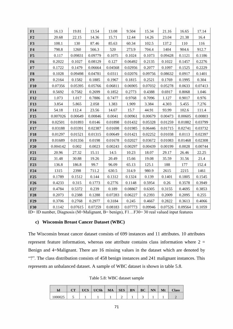
71
F1 16.13 19.81 13.54 13.08 9.504 15.34 21.16 16.65 17.14
F2 20.68 22.15 14.36 15.71 12.44 14.26 23.04 21.38 16.4
F3 108.1 130 87.46 85.63 60.34 102.5 137.2 110 116
F4 798.8 1260 566.3 520 273.9 704.4 1404 904.6 912.7
F5 0.117 0.09831 0.09779 0.1075 0.1024 0.1073 0.09428 0.1121 0.1186
F6 0.2022 0.1027 0.08129 0.127 0.06492 0.2135 0.1022 0.1457 0.2276
F7 0.1722 0.1479 0.06664 0.04568 0.02956 0.2077 0.1097 0.1525 0.2229
F8 0.1028 0.09498 0.04781 0.0311 0.02076 0.09756 0.08632 0.0917 0.1401
F9 0.2164 0.1582 0.1885 0.1967 0.1815 0.2521 0.1769 0.1995 0.304
F10 0.07356 0.05395 0.05766 0.06811 0.06905 0.07032 0.05278 0.0633 0.07413
F11 0.5692 0.7582 0.2699 0.1852 0.2773 0.4388 0.6917 0.8068 1.046
F12 1.073 1.017 0.7886 0.7477 0.9768 0.7096 1.127 0.9017 0.976
F13 3.854 5.865 2.058 1.383 1.909 3.384 4.303 5.455 7.276
F14 54.18 112.4 23.56 14.67 15.7 44.91 93.99 102.6 111.4
F15 0.007026 0.00649 0.00846 0.0041 0.00961 0.00679 0.00473 0.00605 0.00803
F16 0.02501 0.01893 0.0146 0.01898 0.01432 0.05328 0.01259 0.01882 0.03799
F17 0.03188 0.03391 0.02387 0.01698 0.01985 0.06446 0.01715 0.02741 0.03732
F18 0.01297 0.01521 0.01315 0.00649 0.01421 0.02252 0.01038 0.0113 0.02397
F19 0.01689 0.01356 0.0198 0.01678 0.02027 0.03672 0.01083 0.01468 0.02308
F20 0.004142 0.002 0.0023 0.00243 0.00297 0.00439 0.00199 0.0028 0.00744
F21 20.96 27.32 15.11 14.5 10.23 18.07 29.17 26.46 22.25
F22 31.48 30.88 19.26 20.49 15.66 19.08 35.59 31.56 21.4
F23 136.8 186.8 99.7 96.09 65.13 125.1 188 177 152.4
F24 1315 2398 711.2 630.5 314.9 980.9 2615 2215 1461
F25 0.1789 0.1512 0.144 0.1312 0.1324 0.139 0.1401 0.1805 0.1545
F26 0.4233 0.315 0.1773 0.2776 0.1148 0.5954 0.26 0.3578 0.3949
F27 0.4784 0.5372 0.239 0.189 0.08867 0.6305 0.3155 0.4695 0.3853
F28 0.2073 0.2388 0.1288 0.07283 0.06227 0.2393 0.2009 0.2095 0.255
F29 0.3706 0.2768 0.2977 0.3184 0.245 0.4667 0.2822 0.3613 0.4066
F30 0.1142 0.07615 0.07259 0.08183 0.07773 0.09946 0.07526 0.09564 0.1059
ID= ID number, Diagnosis (M=Malignant, B= benign), F1…F30= 30 real valued input features
c) Wisconsin Breast Cancer Dataset (WBC)
The Wisconsin breast cancer dataset consists of 699 instances and 11 attributes. 10 attributes
represent feature information, whereas one attribute contains class information where 2 =
Benign and 4=Malignant. There are 16 missing values in the dataset which are denoted by
―?‖. The class distribution consists of 458 benign instances and 241 malignant instances. This
represents an unbalanced dataset. A sample of WBC dataset is shown in table 5.8.
Table 5.8: WBC dataset sample
Id CT UCS UCSh MA SES BN BC NN Mt Class
1000025 5 1 1 1 2 1 3 1 1 2
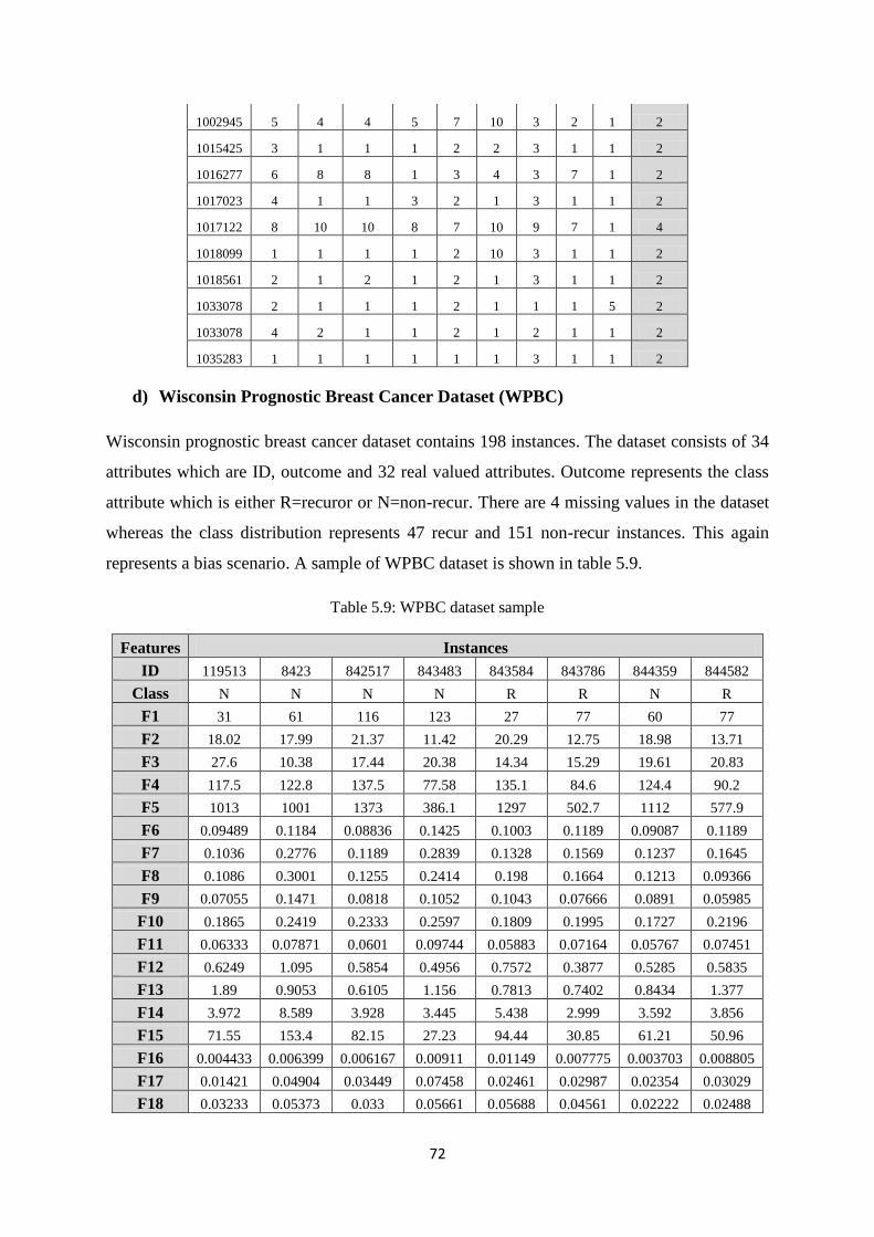
72
1002945 5 4 4 5 7 10 3 2 1 2
1015425 3 1 1 1 2 2 3 1 1 2
1016277 6 8 8 1 3 4 3 7 1 2
1017023 4 1 1 3 2 1 3 1 1 2
1017122 8 10 10 8 7 10 9 7 1 4
1018099 1 1 1 1 2 10 3 1 1 2
1018561 2 1 2 1 2 1 3 1 1 2
1033078 2 1 1 1 2 1 1 1 5 2
1033078 4 2 1 1 2 1 2 1 1 2
1035283 1 1 1 1 1 1 3 1 1 2
d) Wisconsin Prognostic Breast Cancer Dataset (WPBC)
Wisconsin prognostic breast cancer dataset contains 198 instances. The dataset consists of 34
attributes which are ID, outcome and 32 real valued attributes. Outcome represents the class
attribute which is either R=recuror or N=non-recur. There are 4 missing values in the dataset
whereas the class distribution represents 47 recur and 151 non-recur instances. This again
represents a bias scenario. A sample of WPBC dataset is shown in table 5.9.
Table 5.9: WPBC dataset sample
Features Instances
ID 119513 8423 842517 843483 843584 843786 844359 844582
Class N N N N R R N R
F1 31 61 116 123 27 77 60 77
F2 18.02 17.99 21.37 11.42 20.29 12.75 18.98 13.71
F3 27.6 10.38 17.44 20.38 14.34 15.29 19.61 20.83
F4 117.5 122.8 137.5 77.58 135.1 84.6 124.4 90.2
F5 1013 1001 1373 386.1 1297 502.7 1112 577.9
F6 0.09489 0.1184 0.08836 0.1425 0.1003 0.1189 0.09087 0.1189
F7 0.1036 0.2776 0.1189 0.2839 0.1328 0.1569 0.1237 0.1645
F8 0.1086 0.3001 0.1255 0.2414 0.198 0.1664 0.1213 0.09366
F9 0.07055 0.1471 0.0818 0.1052 0.1043 0.07666 0.0891 0.05985
F10 0.1865 0.2419 0.2333 0.2597 0.1809 0.1995 0.1727 0.2196
F11 0.06333 0.07871 0.0601 0.09744 0.05883 0.07164 0.05767 0.07451
F12 0.6249 1.095 0.5854 0.4956 0.7572 0.3877 0.5285 0.5835
F13 1.89 0.9053 0.6105 1.156 0.7813 0.7402 0.8434 1.377
F14 3.972 8.589 3.928 3.445 5.438 2.999 3.592 3.856
F15 71.55 153.4 82.15 27.23 94.44 30.85 61.21 50.96
F16 0.004433 0.006399 0.006167 0.00911 0.01149 0.007775 0.003703 0.008805
F17 0.01421 0.04904 0.03449 0.07458 0.02461 0.02987 0.02354 0.03029
F18 0.03233 0.05373 0.033 0.05661 0.05688 0.04561 0.02222 0.02488
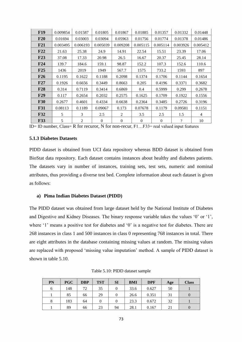
73
F19 0.009854 0.01587 0.01805 0.01867 0.01885 0.01357 0.01332 0.01448
F20 0.01694 0.03003 0.03094 0.05963 0.01756 0.01774 0.01378 0.01486
F21 0.003495 0.006193 0.005039 0.009208 0.005115 0.005114 0.003926 0.005412
F22 21.63 25.38 24.9 14.91 22.54 15.51 23.39 17.06
F23 37.08 17.33 20.98 26.5 16.67 20.37 25.45 28.14
F24 139.7 184.6 159.1 98.87 152.2 107.3 152.6 110.6
F25 1436 2019 1949 567.7 1575 733.2 1593 897
F26 0.1195 0.1622 0.1188 0.2098 0.1374 0.1706 0.1144 0.1654
F27 0.1926 0.6656 0.3449 0.8663 0.205 0.4196 0.3371 0.3682
F28 0.314 0.7119 0.3414 0.6869 0.4 0.5999 0.299 0.2678
F29 0.117 0.2654 0.2032 0.2575 0.1625 0.1709 0.1922 0.1556
F30 0.2677 0.4601 0.4334 0.6638 0.2364 0.3485 0.2726 0.3196
F31 0.08113 0.1189 0.09067 0.173 0.07678 0.1179 0.09581 0.1151
F32 5 3 2.5 2 3.5 2.5 1.5 4
F33 5 2 0 0 0 0 ? 10
ID= ID number, Class= R for recuror, N for non-recur, F1…F33= real valued input features
5.1.3 Diabetes Datasets
PIDD dataset is obtained from UCI data repository whereas BDD dataset is obtained from
BioStat data repository. Each dataset contains instances about healthy and diabetes patients.
The datasets vary in number of instances, training sets, test sets, numeric and nominal
attributes, thus providing a diverse test bed. Complete information about each dataset is given
as follows:
a) Pima Indian Diabetes Dataset (PIDD)
The PIDD dataset was obtained from large dataset held by the National Institute of Diabetes
and Digestive and Kidney Diseases. The binary response variable takes the values ‗0‘ or ‗1‘,
where ‗1‘ means a positive test for diabetes and ‗0‘ is a negative test for diabetes. There are
268 instances in class 1 and 500 instances in class 0 representing 768 instances in total. There
are eight attributes in the database containing missing values at random. The missing values
are replaced with proposed ‗missing value imputation‘ method. A sample of PIDD dataset is
shown in table 5.10.
Table 5.10: PIDD dataset sample
PN PGC DBP TST SI BMI DPF Age Class
6 148 72 35 0 33.6 0.627 50 1
1 85 66 29 0 26.6 0.351 31 0
8 183 64 0 0 23.3 0.672 32 1
1 89 66 23 94 28.1 0.167 21 0
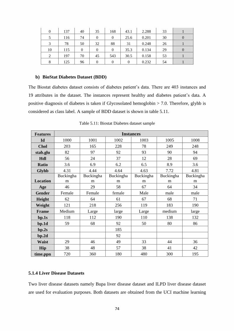
74
0 137 40 35 168 43.1 2.288 33 1
5 116 74 0 0 25.6 0.201 30 0
3 78 50 32 88 31 0.248 26 1
10 115 0 0 0 35.3 0.134 29 0
2 197 70 45 543 30.5 0.158 53 1
8 125 96 0 0 0 0.232 54 1
b) BioStat Diabetes Dataset (BDD)
The Biostat diabetes dataset consists of diabetes patient‘s data. There are 403 instances and
19 attributes in the dataset. The instances represent healthy and diabetes patient‘s data. A
positive diagnosis of diabetes is taken if Glycosolated hemoglobin > 7.0. Therefore, glyhb is
considered as class label. A sample of BDD dataset is shown in table 5.11.
Table 5.11: Biostat Diabetes dataset sample
Features Instances
Id 1000 1001 1002 1003 1005 1008
Chol 203 165 228 78 249 248
stab.glu 82 97 92 93 90 94
Hdl 56 24 37 12 28 69
Ratio 3.6 6.9 6.2 6.5 8.9 3.6
Glyhb 4.31 4.44 4.64 4.63 7.72 4.81
Location
Buckingha
m
Buckingha
m
Buckingha
m
Buckingha
m
Buckingha
m
Buckingha
m
Age 46 29 58 67 64 34
Gender Female Female female Male male male
Height 62 64 61 67 68 71
Weight 121 218 256 119 183 190
Frame Medium Large large Large medium large
bp.1s 118 112 190 110 138 132
bp.1d 59 68 92 50 80 86
bp.2s 185
bp.2d 92
Waist 29 46 49 33 44 36
Hip 38 48 57 38 41 42
time.ppn 720 360 180 480 300 195
5.1.4 Liver Disease Datasets
Two liver disease datasets namely Bupa liver disease dataset and ILPD liver disease dataset
are used for evaluation purposes. Both datasets are obtained from the UCI machine learning
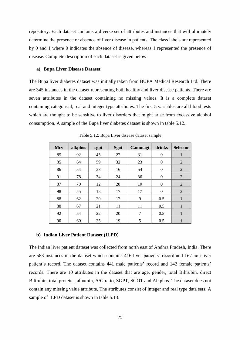
75
repository. Each dataset contains a diverse set of attributes and instances that will ultimately
determine the presence or absence of liver disease in patients. The class labels are represented
by 0 and 1 where 0 indicates the absence of disease, whereas 1 represented the presence of
disease. Complete description of each dataset is given below:
a) Bupa Liver Disease Dataset
The Bupa liver diabetes dataset was initially taken from BUPA Medical Research Ltd. There
are 345 instances in the dataset representing both healthy and liver disease patients. There are
seven attributes in the dataset containing no missing values. It is a complete dataset
containing categorical, real and integer type attributes. The first 5 variables are all blood tests
which are thought to be sensitive to liver disorders that might arise from excessive alcohol
consumption. A sample of the Bupa liver diabetes dataset is shown in table 5.12.
Table 5.12: Bupa Liver disease dataset sample
Mcv alkphos sgpt Sgot Gammagt drinks Selector
85 92 45 27 31 0 1
85 64 59 32 23 0 2
86 54 33 16 54 0 2
91 78 34 24 36 0 2
87 70 12 28 10 0 2
98 55 13 17 17 0 2
88 62 20 17 9 0.5 1
88 67 21 11 11 0.5 1
92 54 22 20 7 0.5 1
90 60 25 19 5 0.5 1
b) Indian Liver Patient Dataset (ILPD)
The Indian liver patient dataset was collected from north east of Andhra Pradesh, India. There
are 583 instances in the dataset which contains 416 liver patients‘ record and 167 non-liver
patient‘s record. The dataset contains 441 male patients‘ record and 142 female patients‘
records. There are 10 attributes in the dataset that are age, gender, total Bilirubin, direct
Bilirubin, total proteins, albumin, A/G ratio, SGPT, SGOT and Alkphos. The dataset does not
contain any missing value attribute. The attributes consist of integer and real type data sets. A
sample of ILPD dataset is shown in table 5.13.

76
Table 5.13: ILPD liver dataset sample
Age Gender TB DB Alkphos Sgpt Sgot TP ALB A/G ratio Selector
65 Female 0.7 0.1 187 16 18 6.8 3.3 0.9 1
62 Male 10.9 5.5 699 64 100 7.5 3.2 0.74 1
62 Male 7.3 4.1 490 60 68 7 3.3 0.89 1
58 Male 1 0.4 182 14 20 6.8 3.4 1 1
72 Male 3.9 2 195 27 59 7.3 2.4 0.4 1
46 Male 1.8 0.7 208 19 14 7.6 4.4 1.3 1
26 Female 0.9 0.2 154 16 12 7 3.5 1 1
29 Female 0.9 0.3 202 14 11 6.7 3.6 1.1 1
17 Male 0.9 0.3 202 22 19 7.4 4.1 1.2 2
55 Male 0.7 0.2 290 53 58 6.8 3.4 1 1
Age=age of patient, Gender=Gender of patient, TB=Total Bilirubin, DB=Direct Bilirubin, Alkphos=
Alkaline Phosphotase, Sgpt= Alamine Aminotransferase, Sgot= Aspartate Aminotransferase, TP=
Total Protiens, ALB= Albumin, A/G ratio= Albumin and Globulin Ratio, Selector= field used to split
the data into two sets
5.1.5 Hepatitis Disease Dataset
The hepatitis disease dataset contains 155 instances in total and is taken from the UCI
machine learning repository. It consists of mostly Boolean or numeric-valued attribute types.
There are 19 attributes in the dataset and some of them contain missing values. The attributes
are consisting of categorical, integer and real type. The missing attribute values are denoted
by ―?‖. These values are replaced with values using proposed missing value imputation
method. A sample of the hepatitis disease dataset is shown in table 5.14.
Table 5.14: Hepatitis dataset sample
C Age S St AV FT ML AN LB LF SP SPD AS VR BB AP SG AL PR H
2 30 2 1 2 2 2 2 1 2 2 2 2 2 1 85 18 4 ? 1
2 50 1 1 2 1 2 2 1 2 2 2 2 2 0.9 135 42 3.5 ? 1
2 78 1 2 2 1 2 2 2 2 2 2 2 2 0.7 96 32 4 ? 1
2 31 1 ? 1 2 2 2 2 2 2 2 2 2 0.7 46 52 4 80 1
2 34 1 2 2 2 2 2 2 2 2 2 2 2 1 ? 200 4 ? 1
2 34 1 2 2 2 2 2 2 2 2 2 2 2 0.9 95 28 4 75 1
1 51 1 1 2 1 2 1 2 2 1 1 2 2 ? ? ? ? ? 1
2 23 1 2 2 2 2 2 2 2 2 2 2 2 1 ? ? ? ? 1
2 39 1 2 2 1 2 2 2 1 2 2 2 2 0.7 ? 48 4.4 ? 1
2 30 1 2 2 2 2 2 2 2 2 2 2 2 1 ? 120 3.9 ? 1
C=Class, Age=Patient‘s age, S=Sex, St= Steroid, AV=Antivirals, FT=Fatigure, ML=Malaise,
AN=Anorexia, LB=Liver Big, LF=Liver Firm, SP=Spleen Palpable, SPD=Spiders, AS=Ascites,
VR=Varices, BB=Bi;irubin, AP=Alk Phosphate, SG=Sgot, AL=Albumin, PR=Protime, H=Histology

77
5.2 Results and Discussion
In this section we will discuss the results of HM-BagMoov framework.
5.2.1 Evaluation Metrics
The performance of proposed multi-layer ensemble framework is measured using Precision,
Recall, F-measure and Accuracy as figures of merit. We have also used confusion metrics,
ANOVA statistical analysis (f-test and p-value) to show the superiority of proposed ensemble
technique as compared with other techniques.
Precision: what % of tuples that the classifier labeled as positive (cancer) are actually
positive (cancer). Mathematically,
Precision =
(5.1)
Recall: Proportion of negative tuples that are correctly identified. Mathematically,
Recall=
(5.2)
F-Measure presents the harmonic mean of both precision and recall. Mathematically,
(5.3)
Accuracy measures the percentage of correct predictions done by the proposed model in
comparison with actual measurements performed on test data. Mathematically,
(5.4)
True positives represents diseased/sick patients correctly diagnosed as diseased/sick
False positive represents healthy people incorrectly identified as sick
True negative represents healthy people correctly identified as healthy
False negative represents sick people incorrectly identified as healthy
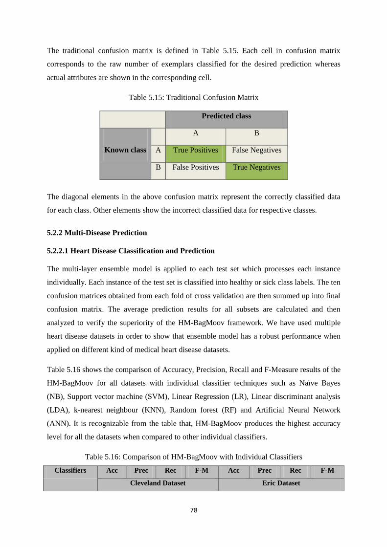
78
The traditional confusion matrix is defined in Table 5.15. Each cell in confusion matrix
corresponds to the raw number of exemplars classified for the desired prediction whereas
actual attributes are shown in the corresponding cell.
Table 5.15: Traditional Confusion Matrix
Predicted class
Known class
A B
A True Positives False Negatives
B False Positives True Negatives
The diagonal elements in the above confusion matrix represent the correctly classified data
for each class. Other elements show the incorrect classified data for respective classes.
5.2.2 Multi-Disease Prediction
5.2.2.1 Heart Disease Classification and Prediction
The multi-layer ensemble model is applied to each test set which processes each instance
individually. Each instance of the test set is classified into healthy or sick class labels. The ten
confusion matrices obtained from each fold of cross validation are then summed up into final
confusion matrix. The average prediction results for all subsets are calculated and then
analyzed to verify the superiority of the HM-BagMoov framework. We have used multiple
heart disease datasets in order to show that ensemble model has a robust performance when
applied on different kind of medical heart disease datasets.
Table 5.16 shows the comparison of Accuracy, Precision, Recall and F-Measure results of the
HM-BagMoov for all datasets with individual classifier techniques such as Naïve Bayes
(NB), Support vector machine (SVM), Linear Regression (LR), Linear discriminant analysis
(LDA), k-nearest neighbour (KNN), Random forest (RF) and Artificial Neural Network
(ANN). It is recognizable from the table that, HM-BagMoov produces the highest accuracy
level for all the datasets when compared to other individual classifiers.
Table 5.16: Comparison of HM-BagMoov with Individual Classifiers
Classifiers Acc Prec Rec F-M Acc Prec Rec F-M
Cleveland Dataset Eric Dataset
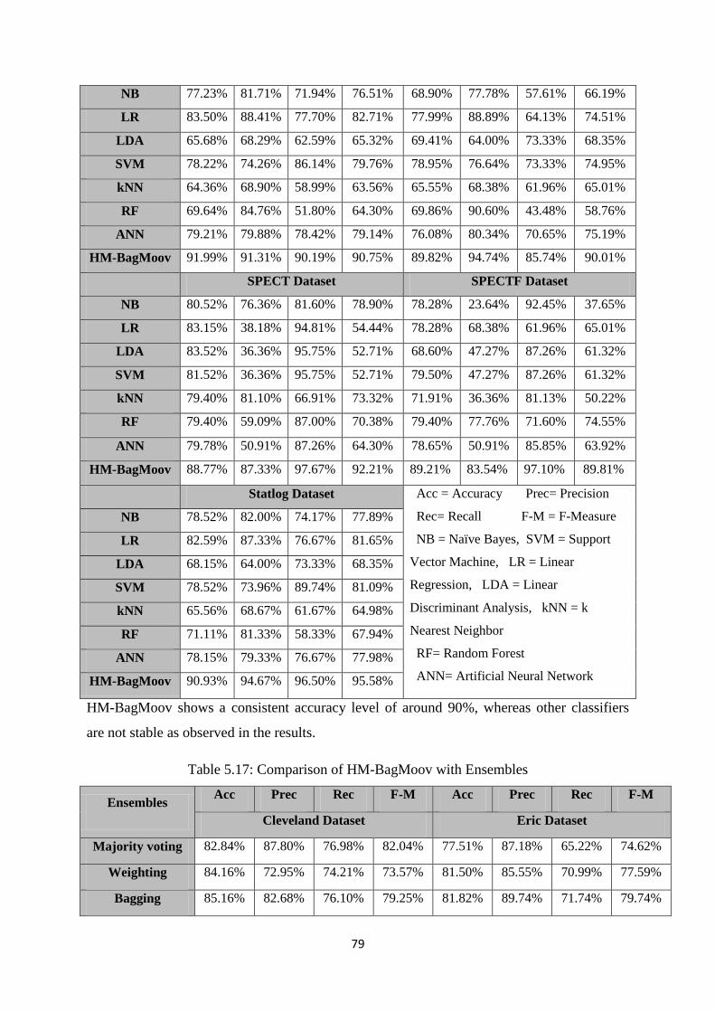
79
NB 77.23% 81.71% 71.94% 76.51% 68.90% 77.78% 57.61% 66.19%
LR 83.50% 88.41% 77.70% 82.71% 77.99% 88.89% 64.13% 74.51%
LDA 65.68% 68.29% 62.59% 65.32% 69.41% 64.00% 73.33% 68.35%
SVM 78.22% 74.26% 86.14% 79.76% 78.95% 76.64% 73.33% 74.95%
kNN 64.36% 68.90% 58.99% 63.56% 65.55% 68.38% 61.96% 65.01%
RF 69.64% 84.76% 51.80% 64.30% 69.86% 90.60% 43.48% 58.76%
ANN 79.21% 79.88% 78.42% 79.14% 76.08% 80.34% 70.65% 75.19%
HM-BagMoov 91.99% 91.31% 90.19% 90.75% 89.82% 94.74% 85.74% 90.01%
SPECT Dataset SPECTF Dataset
NB 80.52% 76.36% 81.60% 78.90% 78.28% 23.64% 92.45% 37.65%
LR 83.15% 38.18% 94.81% 54.44% 78.28% 68.38% 61.96% 65.01%
LDA 83.52% 36.36% 95.75% 52.71% 68.60% 47.27% 87.26% 61.32%
SVM 81.52% 36.36% 95.75% 52.71% 79.50% 47.27% 87.26% 61.32%
kNN 79.40% 81.10% 66.91% 73.32% 71.91% 36.36% 81.13% 50.22%
RF 79.40% 59.09% 87.00% 70.38% 79.40% 77.76% 71.60% 74.55%
ANN 79.78% 50.91% 87.26% 64.30% 78.65% 50.91% 85.85% 63.92%
HM-BagMoov 88.77% 87.33% 97.67% 92.21% 89.21% 83.54% 97.10% 89.81%
Statlog Dataset Acc = Accuracy Prec= Precision
Rec= Recall F-M = F-Measure
NB = Naïve Bayes, SVM = Support
Vector Machine, LR = Linear
Regression, LDA = Linear
Discriminant Analysis, kNN = k
Nearest Neighbor
RF= Random Forest
ANN= Artificial Neural Network
NB 78.52% 82.00% 74.17% 77.89%
LR 82.59% 87.33% 76.67% 81.65%
LDA 68.15% 64.00% 73.33% 68.35%
SVM 78.52% 73.96% 89.74% 81.09%
kNN 65.56% 68.67% 61.67% 64.98%
RF 71.11% 81.33% 58.33% 67.94%
ANN 78.15% 79.33% 76.67% 77.98%
HM-BagMoov 90.93% 94.67% 96.50% 95.58%
HM-BagMoov shows a consistent accuracy level of around 90%, whereas other classifiers
are not stable as observed in the results.
Table 5.17: Comparison of HM-BagMoov with Ensembles
Ensembles Acc Prec Rec F-M Acc Prec Rec F-M
Cleveland Dataset Eric Dataset
Majority voting 82.84% 87.80% 76.98% 82.04% 77.51% 87.18% 65.22% 74.62%
Weighting 84.16% 72.95% 74.21% 73.57% 81.50% 85.55% 70.99% 77.59%
Bagging 85.16% 82.68% 76.10% 79.25% 81.82% 89.74% 71.74% 79.74%
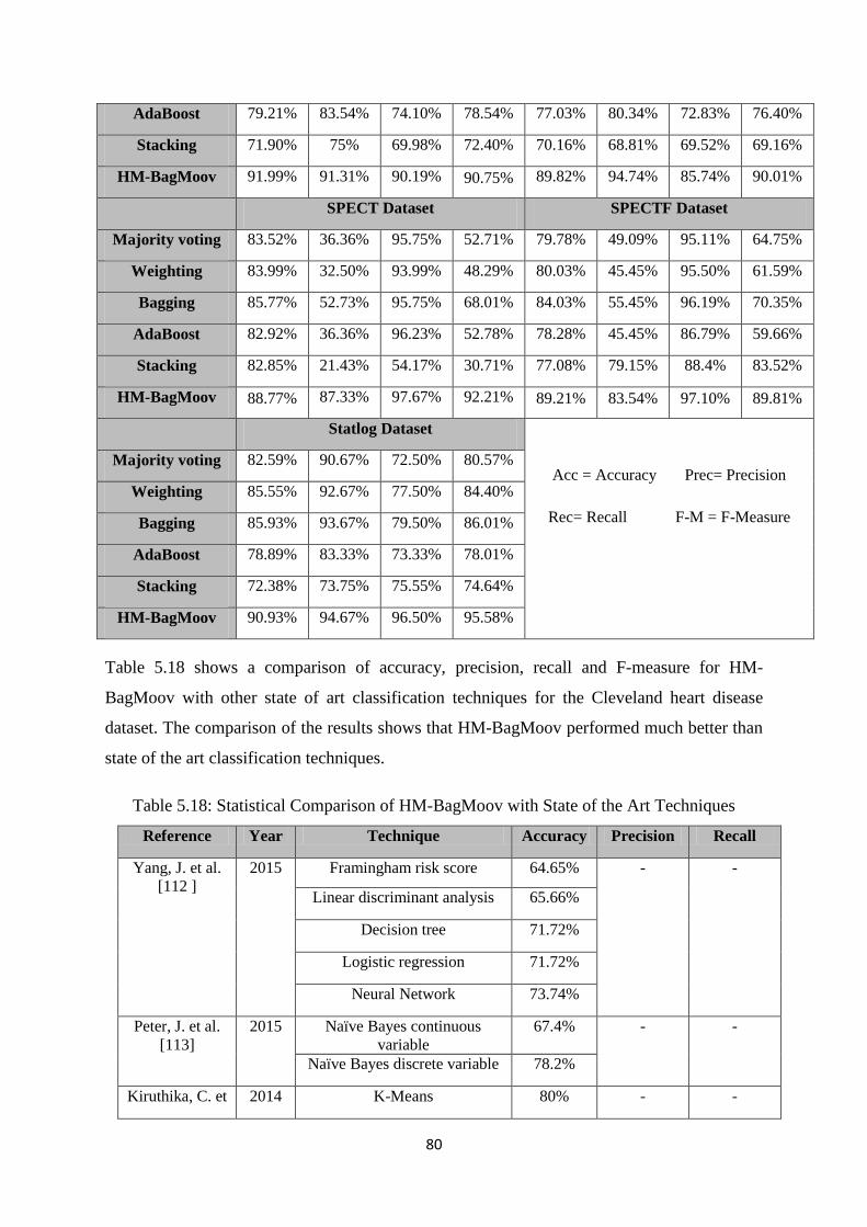
80
AdaBoost 79.21% 83.54% 74.10% 78.54% 77.03% 80.34% 72.83% 76.40%
Stacking 71.90% 75% 69.98% 72.40% 70.16% 68.81% 69.52% 69.16%
HM-BagMoov 91.99% 91.31% 90.19% 90.75% 89.82% 94.74% 85.74% 90.01%
SPECT Dataset SPECTF Dataset
Majority voting 83.52% 36.36% 95.75% 52.71% 79.78% 49.09% 95.11% 64.75%
Weighting 83.99% 32.50% 93.99% 48.29% 80.03% 45.45% 95.50% 61.59%
Bagging 85.77% 52.73% 95.75% 68.01% 84.03% 55.45% 96.19% 70.35%
AdaBoost 82.92% 36.36% 96.23% 52.78% 78.28% 45.45% 86.79% 59.66%
Stacking 82.85% 21.43% 54.17% 30.71% 77.08% 79.15% 88.4% 83.52%
HM-BagMoov 88.77% 87.33% 97.67% 92.21% 89.21% 83.54% 97.10% 89.81%
Statlog Dataset
Acc = Accuracy Prec= Precision
Rec= Recall F-M = F-Measure
Majority voting 82.59% 90.67% 72.50% 80.57%
Weighting 85.55% 92.67% 77.50% 84.40%
Bagging 85.93% 93.67% 79.50% 86.01%
AdaBoost 78.89% 83.33% 73.33% 78.01%
Stacking 72.38% 73.75% 75.55% 74.64%
HM-BagMoov 90.93% 94.67% 96.50% 95.58%
Table 5.18 shows a comparison of accuracy, precision, recall and F-measure for HM-
BagMoov with other state of art classification techniques for the Cleveland heart disease
dataset. The comparison of the results shows that HM-BagMoov performed much better than
state of the art classification techniques.
Table 5.18: Statistical Comparison of HM-BagMoov with State of the Art Techniques
Reference Year Technique Accuracy Precision Recall
Yang, J. et al.
[112 ]
2015 Framingham risk score 64.65% - -
Linear discriminant analysis 65.66%
Decision tree 71.72%
Logistic regression 71.72%
Neural Network 73.74%
Peter, J. et al.
[113]
2015 Naïve Bayes continuous
variable
67.4% - -
Naïve Bayes discrete variable 78.2%
Kiruthika, C. et 2014 K-Means 80% - -
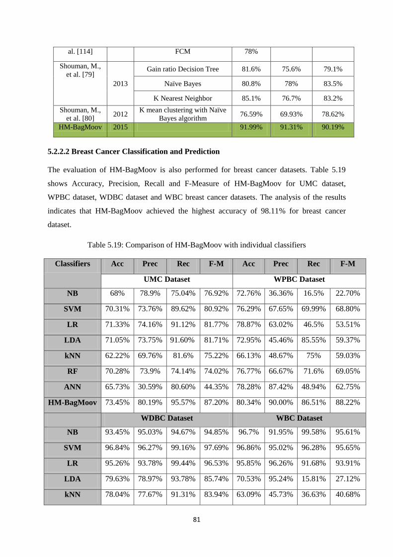
81
al. [114] FCM 78%
Shouman, M.,
et al. [79]
2013
Gain ratio Decision Tree 81.6% 75.6% 79.1%
Naïve Bayes 80.8% 78% 83.5%
K Nearest Neighbor 85.1% 76.7% 83.2%
Shouman, M.,
et al. [80] 2012
K mean clustering with Naïve
Bayes algorithm 76.59% 69.93% 78.62%
HM-BagMoov 2015 91.99% 91.31% 90.19%
5.2.2.2 Breast Cancer Classification and Prediction
The evaluation of HM-BagMoov is also performed for breast cancer datasets. Table 5.19
shows Accuracy, Precision, Recall and F-Measure of HM-BagMoov for UMC dataset,
WPBC dataset, WDBC dataset and WBC breast cancer datasets. The analysis of the results
indicates that HM-BagMoov achieved the highest accuracy of 98.11% for breast cancer
dataset.
Table 5.19: Comparison of HM-BagMoov with individual classifiers
Classifiers Acc Prec Rec F-M Acc Prec Rec F-M
UMC Dataset WPBC Dataset
NB 68% 78.9% 75.04% 76.92% 72.76% 36.36% 16.5% 22.70%
SVM 70.31% 73.76% 89.62% 80.92% 76.29% 67.65% 69.99% 68.80%
LR 71.33% 74.16% 91.12% 81.77% 78.87% 63.02% 46.5% 53.51%
LDA 71.05% 73.75% 91.60% 81.71% 72.95% 45.46% 85.55% 59.37%
kNN 62.22% 69.76% 81.6% 75.22% 66.13% 48.67% 75% 59.03%
RF 70.28% 73.9% 74.14% 74.02% 76.77% 66.67% 71.6% 69.05%
ANN 65.73% 30.59% 80.60% 44.35% 78.28% 87.42% 48.94% 62.75%
HM-BagMoov 73.45% 80.19% 95.57% 87.20% 80.34% 90.00% 86.51% 88.22%
WDBC Dataset WBC Dataset
NB 93.45% 95.03% 94.67% 94.85% 96.7% 91.95% 99.58% 95.61%
SVM 96.84% 96.27% 99.16% 97.69% 96.86% 95.02% 96.28% 95.65%
LR 95.26% 93.78% 99.44% 96.53% 95.85% 96.26% 91.68% 93.91%
LDA 79.63% 78.97% 93.78% 85.74% 70.53% 95.24% 15.81% 27.12%
kNN 78.04% 77.67% 91.31% 83.94% 63.09% 45.73% 36.63% 40.68%
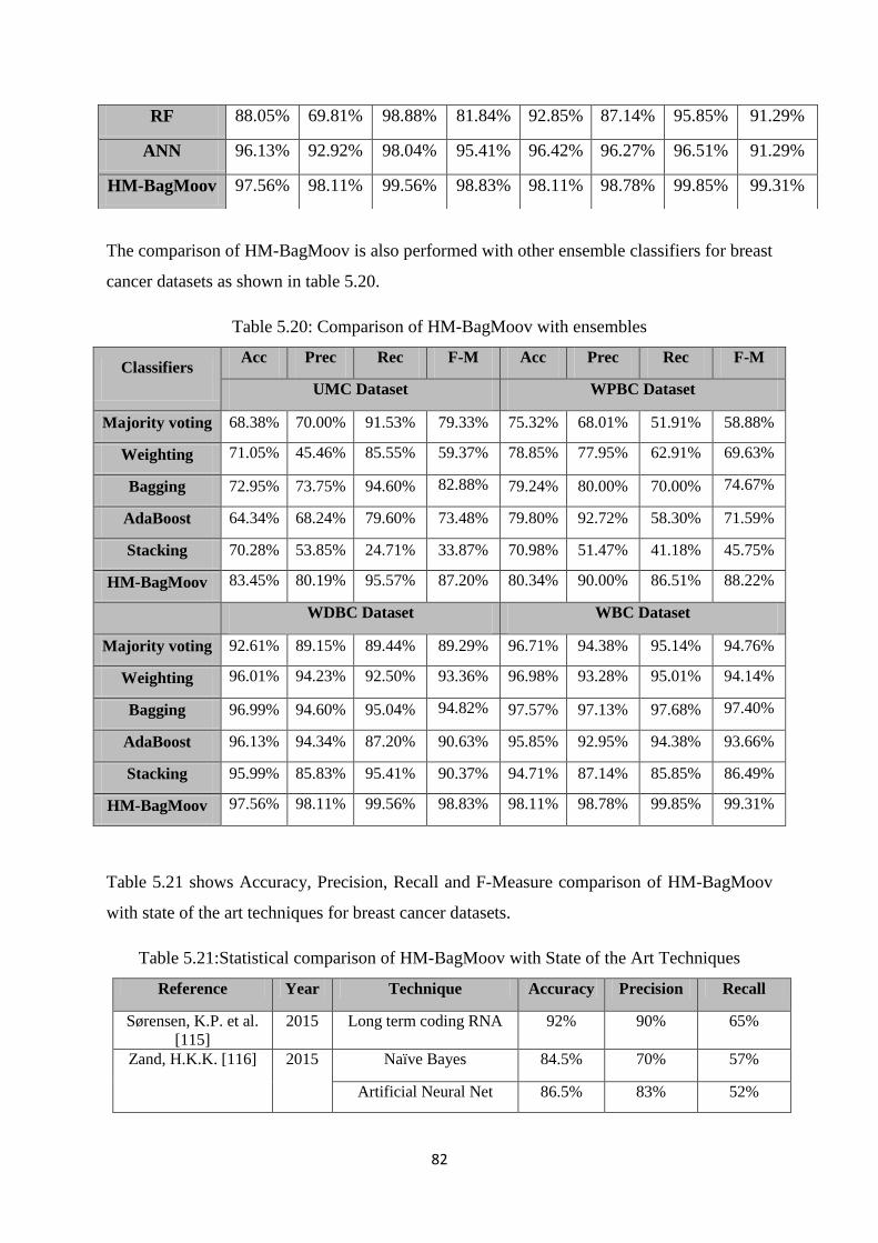
82
The comparison of HM-BagMoov is also performed with other ensemble classifiers for breast
cancer datasets as shown in table 5.20.
Table 5.20: Comparison of HM-BagMoov with ensembles
Classifiers Acc Prec Rec F-M Acc Prec Rec F-M
UMC Dataset WPBC Dataset
Majority voting 68.38% 70.00% 91.53% 79.33% 75.32% 68.01% 51.91% 58.88%
Weighting 71.05% 45.46% 85.55% 59.37% 78.85% 77.95% 62.91% 69.63%
Bagging 72.95% 73.75% 94.60% 82.88% 79.24% 80.00% 70.00% 74.67%
AdaBoost 64.34% 68.24% 79.60% 73.48% 79.80% 92.72% 58.30% 71.59%
Stacking 70.28% 53.85% 24.71% 33.87% 70.98% 51.47% 41.18% 45.75%
HM-BagMoov 83.45% 80.19% 95.57% 87.20% 80.34% 90.00% 86.51% 88.22%
WDBC Dataset WBC Dataset
Majority voting 92.61% 89.15% 89.44% 89.29% 96.71% 94.38% 95.14% 94.76%
Weighting 96.01% 94.23% 92.50% 93.36% 96.98% 93.28% 95.01% 94.14%
Bagging 96.99% 94.60% 95.04% 94.82% 97.57% 97.13% 97.68% 97.40%
AdaBoost 96.13% 94.34% 87.20% 90.63% 95.85% 92.95% 94.38% 93.66%
Stacking 95.99% 85.83% 95.41% 90.37% 94.71% 87.14% 85.85% 86.49%
HM-BagMoov 97.56% 98.11% 99.56% 98.83% 98.11% 98.78% 99.85% 99.31%
Table 5.21 shows Accuracy, Precision, Recall and F-Measure comparison of HM-BagMoov
with state of the art techniques for breast cancer datasets.
Table 5.21:Statistical comparison of HM-BagMoov with State of the Art Techniques
Reference Year Technique Accuracy Precision Recall
Sørensen, K.P. et al.
[115]
2015 Long term coding RNA 92% 90% 65%
Zand, H.K.K. [116] 2015 Naïve Bayes 84.5% 70% 57%
Artificial Neural Net 86.5% 83% 52%
RF 88.05% 69.81% 98.88% 81.84% 92.85% 87.14% 95.85% 91.29%
ANN 96.13% 92.92% 98.04% 95.41% 96.42% 96.27% 96.51% 91.29%
HM-BagMoov 97.56% 98.11% 99.56% 98.83% 98.11% 98.78% 99.85% 99.31%
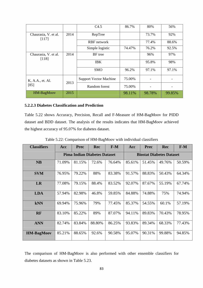
83
C4.5 86.7% 80% 56%
Chaurasia, V. et al.
[117]
2014 RepTree 73.7% 92%
RBF network 77.4% 88.6%
Simple logistic 74.47% 76.2% 92.5%
Chaurasia, V. et al.
[118]
2014 BF tree 96% 97%
IBK 95.8% 98%
SMO 96.2% 97.1% 97.1%
K, A.A., et. Al.
[85] 2013
Support Vector Machine 75.00% - -
Random forest 75.00% - -
HM-BagMoov 2015 98.11% 98.78% 99.85%
5.2.2.3 Diabetes Classification and Prediction
Table 5.22 shows Accuracy, Precision, Recall and F-Measure of HM-BagMoov for PIDD
dataset and BDD dataset. The analysis of the results indicates that HM-BagMoov achieved
the highest accuracy of 95.07% for diabetes dataset.
Table 5.22: Comparison of HM-BagMoov with individual classifiers
Classifiers Acc Prec Rec F-M Acc Prec Rec F-M
Pima Indian Diabetes Dataset Biostat Diabetes Dataset
NB 71.09% 81.15% 72.6% 76.64% 85.61% 51.45% 49.76% 50.59%
SVM 76.95% 79.22% 88% 83.38% 91.57% 88.83% 50.43% 64.34%
LR 77.08% 79.15% 88.4% 83.52% 92.07% 87.67% 55.19% 67.74%
LDA 57.94% 82.98% 46.8% 59.85% 84.88% 74.88% 75% 74.94%
kNN 69.94% 75.96% 79% 77.45% 85.37% 54.55% 60.1% 57.19%
RF 83.10% 85.22% 89% 87.07% 94.11% 89.83% 70.43% 78.95%
ANN 82.74% 83.84% 88.80% 86.25% 93.83% 89.34% 68.33% 77.43%
HM-BagMoov 85.21% 88.65% 92.6% 90.58% 95.07% 90.31% 99.88% 94.85%
The comparison of HM-BagMoov is also performed with other ensemble classifiers for
diabetes datasets as shown in Table 5.23.
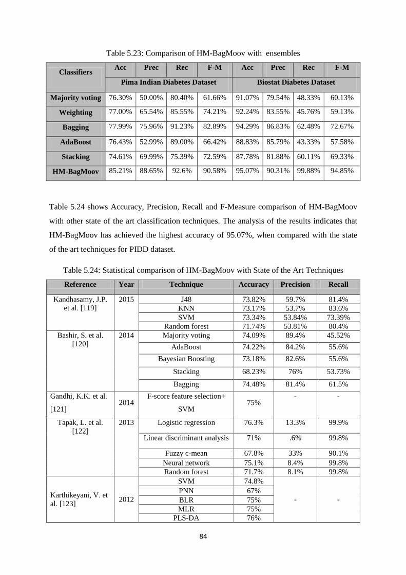
84
Table 5.23: Comparison of HM-BagMoov with ensembles
Classifiers Acc Prec Rec F-M Acc Prec Rec F-M
Pima Indian Diabetes Dataset Biostat Diabetes Dataset
Majority voting 76.30% 50.00% 80.40% 61.66% 91.07% 79.54% 48.33% 60.13%
Weighting 77.00% 65.54% 85.55% 74.21% 92.24% 83.55% 45.76% 59.13%
Bagging 77.99% 75.96% 91.23% 82.89% 94.29% 86.83% 62.48% 72.67%
AdaBoost 76.43% 52.99% 89.00% 66.42% 88.83% 85.79% 43.33% 57.58%
Stacking 74.61% 69.99% 75.39% 72.59% 87.78% 81.88% 60.11% 69.33%
HM-BagMoov 85.21% 88.65% 92.6% 90.58% 95.07% 90.31% 99.88% 94.85%
Table 5.24 shows Accuracy, Precision, Recall and F-Measure comparison of HM-BagMoov
with other state of the art classification techniques. The analysis of the results indicates that
HM-BagMoov has achieved the highest accuracy of 95.07%, when compared with the state
of the art techniques for PIDD dataset.
Table 5.24: Statistical comparison of HM-BagMoov with State of the Art Techniques
Reference Year Technique Accuracy Precision Recall
Kandhasamy, J.P.
et al. [119]
2015 J48 73.82% 59.7% 81.4%
KNN 73.17% 53.7% 83.6%
SVM 73.34% 53.84% 73.39%
Random forest 71.74% 53.81% 80.4%
Bashir, S. et al.
[120]
2014 Majority voting 74.09% 89.4% 45.52%
AdaBoost 74.22% 84.2% 55.6%
Bayesian Boosting 73.18% 82.6% 55.6%
Stacking 68.23% 76% 53.73%
Bagging 74.48% 81.4% 61.5%
Gandhi, K.K. et al.
[121] 2014
F-score feature selection+
SVM 75%
- -
Tapak, L. et al.
[122]
2013 Logistic regression 76.3% 13.3% 99.9%
Linear discriminant analysis 71% .6% 99.8%
Fuzzy c-mean 67.8% 33% 90.1%
Neural network 75.1% 8.4% 99.8%
Random forest 71.7% 8.1% 99.8%
Karthikeyani, V. et
al. [123] 2012
SVM 74.8%
- -
PNN 67%
BLR 75%
MLR 75%
PLS-DA 76%
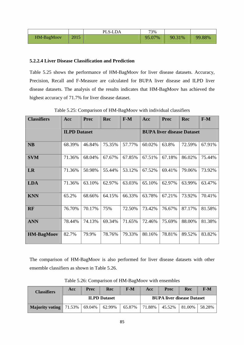
85
PLS-LDA 73%
HM-BagMoov 2015 95.07% 90.31% 99.88%
5.2.2.4 Liver Disease Classification and Prediction
Table 5.25 shows the performance of HM-BagMoov for liver disease datasets. Accuracy,
Precision, Recall and F-Measure are calculated for BUPA liver disease and ILPD liver
disease datasets. The analysis of the results indicates that HM-BagMoov has achieved the
highest accuracy of 71.7% for liver disease dataset.
Table 5.25: Comparison of HM-BagMoov with individual classifiers
Classifiers Acc Prec Rec F-M Acc Prec Rec F-M
ILPD Dataset BUPA liver disease Dataset
NB 68.39% 46.84% 75.35% 57.77% 60.02% 63.8% 72.59% 67.91%
SVM 71.36% 68.04% 67.67% 67.85% 67.51% 67.18% 86.02% 75.44%
LR 71.36% 50.98% 55.44% 53.12% 67.52% 69.41% 79.06% 73.92%
LDA 71.36% 63.10% 62.97% 63.03% 65.10% 62.97% 63.99% 63.47%
KNN 65.2% 68.66% 64.15% 66.33% 63.78% 67.21% 73.92% 70.41%
RF 76.70% 70.17% 75% 72.50% 73.42% 76.67% 87.17% 81.58%
ANN 78.44% 74.13% 69.34% 71.65% 72.46% 75.69% 88.00% 81.38%
HM-BagMoov 82.7% 79.9% 78.76% 79.33% 80.16% 78.81% 89.52% 83.82%
The comparison of HM-BagMoov is also performed for liver disease datasets with other
ensemble classifiers as shown in Table 5.26.
Table 5.26: Comparison of HM-BagMoov with ensembles
Classifiers Acc Prec Rec F-M Acc Prec Rec F-M
ILPD Dataset BUPA liver disease Dataset
Majority voting 71.53% 69.04% 62.99% 65.87% 71.88% 45.52% 81.00% 58.28%
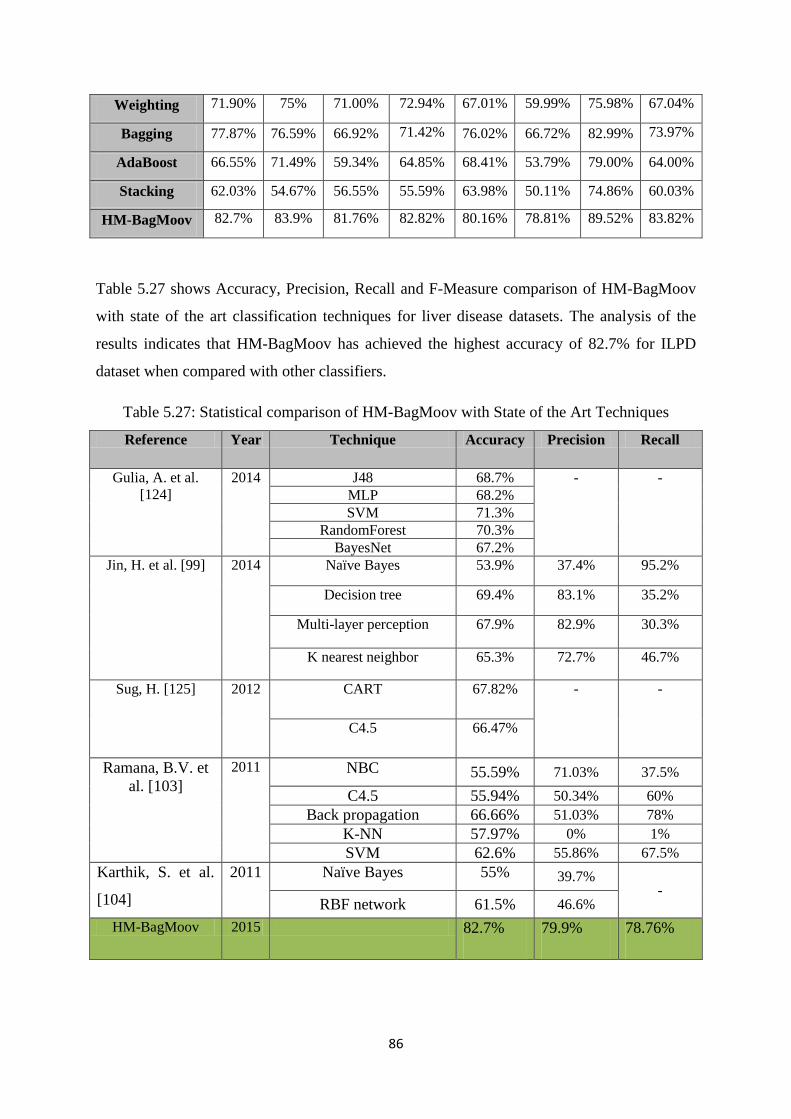
86
Weighting 71.90% 75% 71.00% 72.94% 67.01% 59.99% 75.98% 67.04%
Bagging 77.87% 76.59% 66.92% 71.42% 76.02% 66.72% 82.99% 73.97%
AdaBoost 66.55% 71.49% 59.34% 64.85% 68.41% 53.79% 79.00% 64.00%
Stacking 62.03% 54.67% 56.55% 55.59% 63.98% 50.11% 74.86% 60.03%
HM-BagMoov 82.7% 83.9% 81.76% 82.82% 80.16% 78.81% 89.52% 83.82%
Table 5.27 shows Accuracy, Precision, Recall and F-Measure comparison of HM-BagMoov
with state of the art classification techniques for liver disease datasets. The analysis of the
results indicates that HM-BagMoov has achieved the highest accuracy of 82.7% for ILPD
dataset when compared with other classifiers.
Table 5.27: Statistical comparison of HM-BagMoov with State of the Art Techniques
Reference Year Technique Accuracy Precision Recall
Gulia, A. et al.
[124]
2014 J48 68.7% - -
MLP 68.2%
SVM 71.3%
RandomForest 70.3%
BayesNet 67.2%
Jin, H. et al. [99] 2014 Naïve Bayes 53.9% 37.4% 95.2%
Decision tree 69.4% 83.1% 35.2%
Multi-layer perception 67.9% 82.9% 30.3%
K nearest neighbor 65.3% 72.7% 46.7%
Sug, H. [125] 2012 CART 67.82% - -
C4.5 66.47%
Ramana, B.V. et
al. [103]
2011 NBC 55.59% 71.03% 37.5%
C4.5 55.94% 50.34% 60%
Back propagation 66.66% 51.03% 78%
K-NN 57.97% 0% 1%
SVM 62.6% 55.86% 67.5%
Karthik, S. et al.
[104]
2011 Naïve Bayes 55% 39.7% -
RBF network 61.5% 46.6%
HM-BagMoov 2015 82.7% 79.9% 78.76%
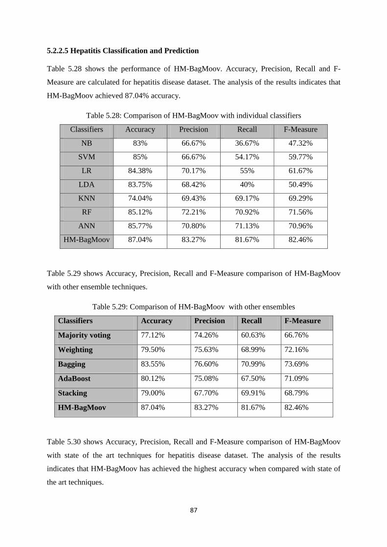
87
5.2.2.5 Hepatitis Classification and Prediction
Table 5.28 shows the performance of HM-BagMoov. Accuracy, Precision, Recall and F-
Measure are calculated for hepatitis disease dataset. The analysis of the results indicates that
HM-BagMoov achieved 87.04% accuracy.
Table 5.28: Comparison of HM-BagMoov with individual classifiers
Classifiers Accuracy Precision Recall F-Measure
NB 83% 66.67% 36.67% 47.32%
SVM 85% 66.67% 54.17% 59.77%
LR 84.38% 70.17% 55% 61.67%
LDA 83.75% 68.42% 40% 50.49%
KNN 74.04% 69.43% 69.17% 69.29%
RF 85.12% 72.21% 70.92% 71.56%
ANN 85.77% 70.80% 71.13% 70.96%
HM-BagMoov 87.04% 83.27% 81.67% 82.46%
Table 5.29 shows Accuracy, Precision, Recall and F-Measure comparison of HM-BagMoov
with other ensemble techniques.
Table 5.29: Comparison of HM-BagMoov with other ensembles
Classifiers Accuracy Precision Recall F-Measure
Majority voting 77.12% 74.26% 60.63% 66.76%
Weighting 79.50% 75.63% 68.99% 72.16%
Bagging 83.55% 76.60% 70.99% 73.69%
AdaBoost 80.12% 75.08% 67.50% 71.09%
Stacking 79.00% 67.70% 69.91% 68.79%
HM-BagMoov 87.04% 83.27% 81.67% 82.46%
Table 5.30 shows Accuracy, Precision, Recall and F-Measure comparison of HM-BagMoov
with state of the art techniques for hepatitis disease dataset. The analysis of the results
indicates that HM-BagMoov has achieved the highest accuracy when compared with state of
the art techniques.
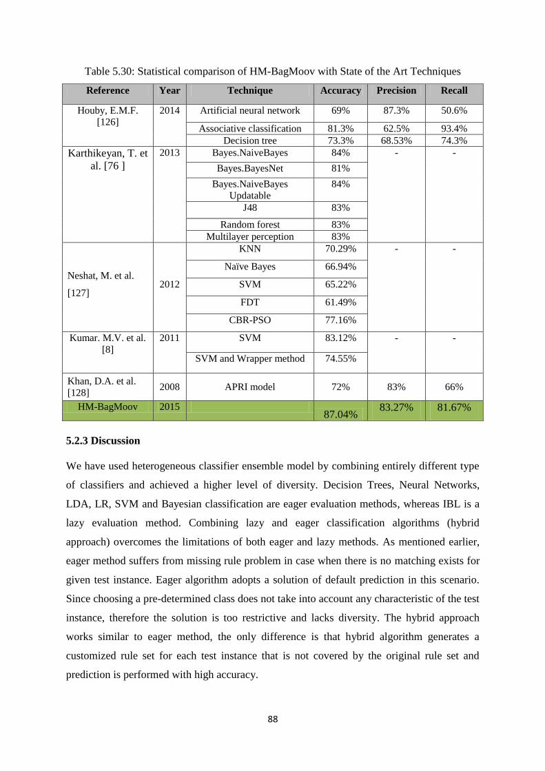
88
Table 5.30: Statistical comparison of HM-BagMoov with State of the Art Techniques
Reference Year Technique Accuracy Precision Recall
Houby, E.M.F.
[126]
2014 Artificial neural network 69% 87.3% 50.6%
Associative classification 81.3% 62.5% 93.4%
Decision tree 73.3% 68.53% 74.3%
Karthikeyan, T. et
al. [76 ]
2013 Bayes.NaiveBayes 84% - -
Bayes.BayesNet 81%
Bayes.NaiveBayes
Updatable
84%
J48 83%
Random forest 83%
Multilayer perception 83%
Neshat, M. et al.
[127] 2012
KNN 70.29% - -
Naïve Bayes 66.94%
SVM 65.22%
FDT 61.49%
CBR-PSO 77.16%
Kumar. M.V. et al.
[8]
2011 SVM 83.12% - -
SVM and Wrapper method 74.55%
Khan, D.A. et al.
[128] 2008 APRI model 72% 83% 66%
HM-BagMoov 2015 87.04%
83.27% 81.67%
5.2.3 Discussion
We have used heterogeneous classifier ensemble model by combining entirely different type
of classifiers and achieved a higher level of diversity. Decision Trees, Neural Networks,
LDA, LR, SVM and Bayesian classification are eager evaluation methods, whereas IBL is a
lazy evaluation method. Combining lazy and eager classification algorithms (hybrid
approach) overcomes the limitations of both eager and lazy methods. As mentioned earlier,
eager method suffers from missing rule problem in case when there is no matching exists for
given test instance. Eager algorithm adopts a solution of default prediction in this scenario.
Since choosing a pre-determined class does not take into account any characteristic of the test
instance, therefore the solution is too restrictive and lacks diversity. The hybrid approach
works similar to eager method, the only difference is that hybrid algorithm generates a
customized rule set for each test instance that is not covered by the original rule set and
prediction is performed with high accuracy.

89
Moreover the diversity parameter can be determined by the extent to which each individual
classifier disagrees about the probability distributions for the test datasets. The individual
Naïve Bayes classifier considers each attribute independently without taking into account the
relation between them, whereas HM-BagMoov model can handle dependency and relations
between given attribute set. The linear regression classifier and linear discriminant analysis
are used in HM-BagMoov model in order to perform correlation analysis between attribute
sets as functional dependencies exist between input variables. Thus HM-BagMoov model
resolves the limitation of individual Naïve Bayes classifier by handling correlation. The
individual IBL algorithm has various limitations such as it is computationally intensive and
requires lots of storage space. The HM-BagMoov model has resolved the storage problem by
selecting only necessary and useful features for disease analysis and prediction. The SVM
algorithm performs the feature selection by using only subset of data chosen based on
information gain. Moreover SVM algorithm decreases the overfitting issue and increase the
prediction and classification accuracy. Thus, all of the selected classifiers complement each
other very well. In any scenario where one classifier has some limitation, the other classifier
overcomes it and as a result higher ensemble performance is achieved.
5.2.4 ANOVA Statistics
Another method used to show the significance of the results is ANOVA (Analysis of
Variance) statistics. It is a statistical test used to measure the difference between group means
and their variations such as variations among and between groups. f-test is used to measure
the total deviation pattern based on same datasets. The result of f-test indicates the model that
best fits to the given dataset. The f-test is also used to assess whether the expected values of
given datasets are different from the values predicted by other classifier and is represented by
ANOVA f-test. Following formula is used to calculate the f-test statistics:
(5.5)
The SS, df, MS, F, F crit and P-value are calculated in ANOVA statistics. SS stands for sum
of squares and is calculated between group SS(B) and within group SS(W) using the
following formulas:
∑
(5.6)
(5.7)
yvariabilitgroupwithin
yvariabilitgroupbetweenF
2
df.sSS(W)

90
where x is total values whereas X is the mean of values and s is standard deviation. The df
stands for degree of freedom. It is the sum of degrees of freedom for all individual samples.
df=N-k (5.8)
where k is sample size and total degrees of freedom is k less than the total sample size. MS
stands for mean square and is calculated for between group MS(B) and within group MS(W).
The MS(B) is calculated by dividing the SS(B) by its degrees of freedom. MS(W) is
calculated by dividing the SS(W) by its degrees of freedom. The F crit is critical value of F
which is a function of the numerator degree of freedom, denominator degree of freedom and
significance level α=0.05.
It is always good to have f-ratio greater than f-critical value because if this value is large
enough, then we can reject the null hypothesis in favor of the principal that the classifiers we
are comparing really do differ from each other. We have calculated the f-ratio and f-critical
for each individual classifier versus proposed ensemble for all datasets. The smaller value of
f-critical favors the high performance of ensemble framework. Moreover, the p-value is
calculated for 95% confidence interval. It is observed from the results that p value is well
below the chosen alpha of 0.05. It also rejects the null hypothesis in support of the conclusion
that proposed ensemble classifier outperforms other classifiers for almost all the datasets.
The results of ANOVA statistics for each dataset are shown in Table 5.31-5.44. The analysis
of ANOVA statistics shows that HM-BagMoov framework results are statistically significant.
Table 12 shows the ANOVA statistics of HM-BagMoov against each individual classifier for
the Cleveland heart disease dataset. Each individual classifier is evaluated against HM-
BagMoov and calculations are performed for ‗Between Groups‘ and ‗Within Groups‘
variables. The analysis of the results indicates that F-ratio is greater than F-critical for all
classifiers which represents high performance of HM-BagMoov. Moreover, p-value for each
classifier is smaller than 0.01 which shows significant results. Table 13 shows a comparison
of ANOVA statistics for SPECT dataset. F ratio, F critical and P-value shows the significance
of results where F-critical and F ratio are compared for each classifier. The ANOVA statistics
for each dataset is shown below.
5.2.4.1 Heart Disease Datasets
Table 5.31-5.35 shows the ANOVA statistics results for HM-BagMoov ensemble classifier
when compared with each individual classifier for heart disease datasets. The f-ratio and p-
value obtained from ANOVA statistics indicate that the results are extremely statistically
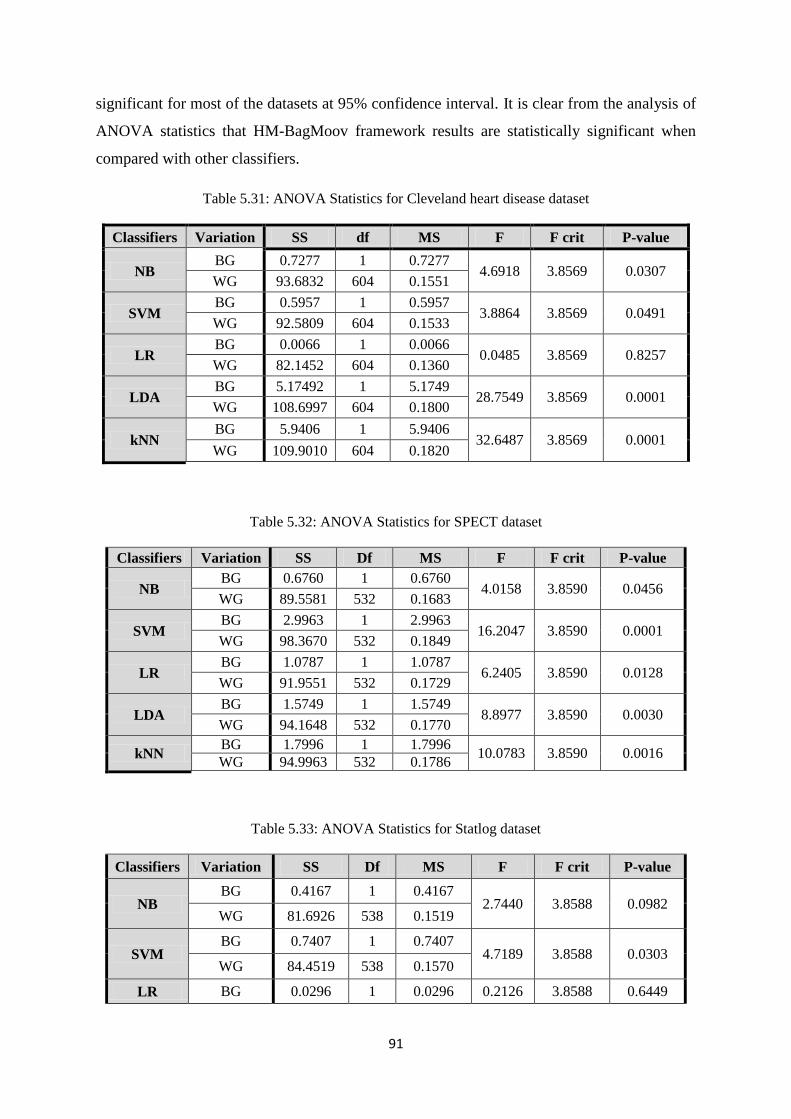
91
significant for most of the datasets at 95% confidence interval. It is clear from the analysis of
ANOVA statistics that HM-BagMoov framework results are statistically significant when
compared with other classifiers.
Table 5.31: ANOVA Statistics for Cleveland heart disease dataset
Classifiers Variation SS df MS F F crit P-value
NB BG 0.7277 1 0.7277
4.6918 3.8569 0.0307 WG 93.6832 604 0.1551
SVM BG 0.5957 1 0.5957
3.8864 3.8569 0.0491 WG 92.5809 604 0.1533
LR BG 0.0066 1 0.0066
0.0485 3.8569 0.8257 WG 82.1452 604 0.1360
LDA BG 5.17492 1 5.1749
28.7549 3.8569 0.0001 WG 108.6997 604 0.1800
kNN BG 5.9406 1 5.9406
32.6487 3.8569 0.0001 WG 109.9010 604 0.1820
Table 5.32: ANOVA Statistics for SPECT dataset
Classifiers Variation SS Df MS F F crit P-value
NB BG 0.6760 1 0.6760
4.0158 3.8590 0.0456 WG 89.5581 532 0.1683
SVM BG 2.9963 1 2.9963
16.2047 3.8590 0.0001 WG 98.3670 532 0.1849
LR BG 1.0787 1 1.0787
6.2405 3.8590 0.0128 WG 91.9551 532 0.1729
LDA BG 1.5749 1 1.5749
8.8977 3.8590 0.0030 WG 94.1648 532 0.1770
kNN BG 1.7996 1 1.7996
10.0783 3.8590 0.0016 WG 94.9963 532 0.1786
Table 5.33: ANOVA Statistics for Statlog dataset
Classifiers Variation SS Df MS F F crit P-value
NB BG 0.4167 1 0.4167
2.7440 3.8588 0.0982 WG 81.6926 538 0.1519
SVM BG 0.7407 1 0.7407
4.7189 3.8588 0.0303 WG 84.4519 538 0.1570
LR BG 0.0296 1 0.0296 0.2126 3.8588 0.6449
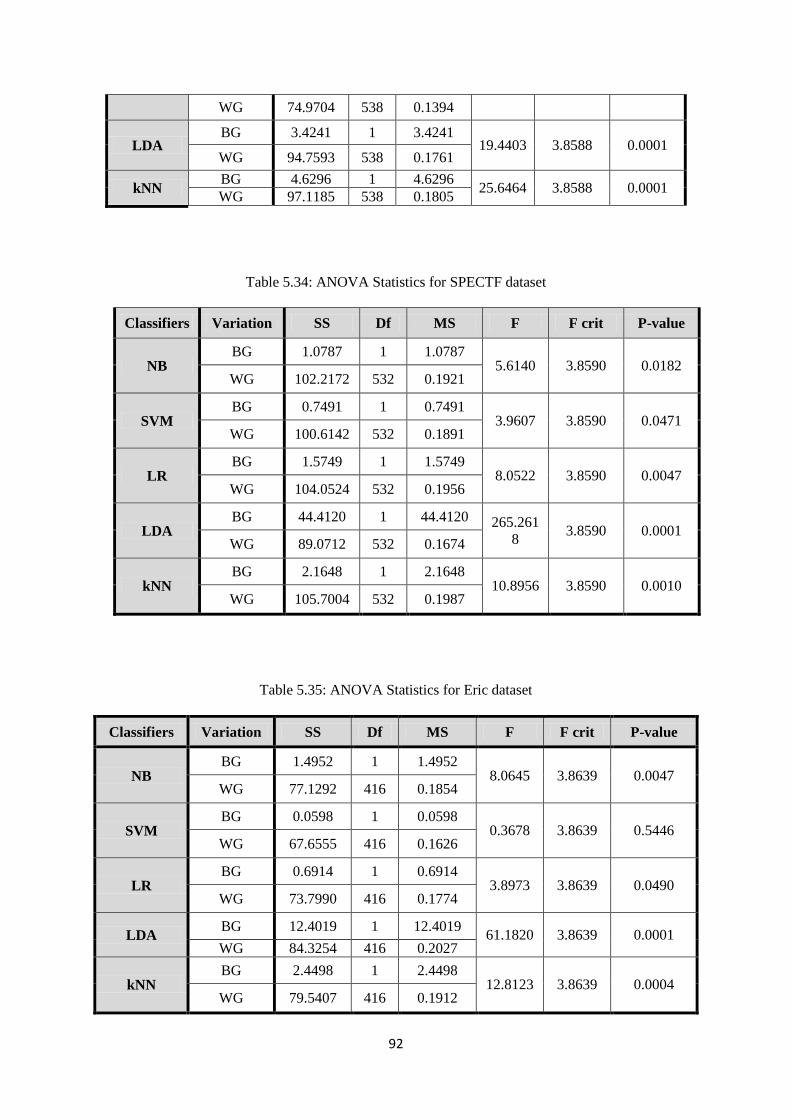
92
WG 74.9704 538 0.1394
LDA BG 3.4241 1 3.4241
19.4403 3.8588 0.0001 WG 94.7593 538 0.1761
kNN BG 4.6296 1 4.6296
25.6464 3.8588 0.0001 WG 97.1185 538 0.1805
Table 5.34: ANOVA Statistics for SPECTF dataset
Classifiers Variation SS Df MS F F crit P-value
NB BG 1.0787 1 1.0787
5.6140 3.8590 0.0182 WG 102.2172 532 0.1921
SVM BG 0.7491 1 0.7491
3.9607 3.8590 0.0471 WG 100.6142 532 0.1891
LR BG 1.5749 1 1.5749
8.0522 3.8590 0.0047 WG 104.0524 532 0.1956
LDA BG 44.4120 1 44.4120 265.261
8 3.8590 0.0001
WG 89.0712 532 0.1674
kNN BG 2.1648 1 2.1648
10.8956 3.8590 0.0010 WG 105.7004 532 0.1987
Table 5.35: ANOVA Statistics for Eric dataset
Classifiers Variation SS Df MS F F crit P-value
NB BG 1.4952 1 1.4952
8.0645 3.8639 0.0047 WG 77.1292 416 0.1854
SVM BG 0.0598 1 0.0598
0.3678 3.8639 0.5446 WG 67.6555 416 0.1626
LR BG 0.6914 1 0.6914
3.8973 3.8639 0.0490 WG 73.7990 416 0.1774
LDA BG 12.4019 1 12.4019
61.1820 3.8639 0.0001 WG 84.3254 416 0.2027
kNN BG 2.4498 1 2.4498
12.8123 3.8639 0.0004 WG 79.5407 416 0.1912
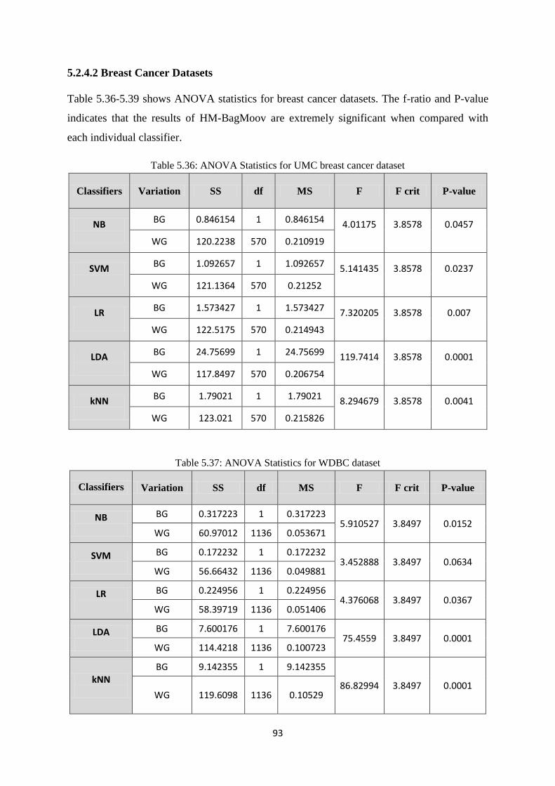
93
5.2.4.2 Breast Cancer Datasets
Table 5.36-5.39 shows ANOVA statistics for breast cancer datasets. The f-ratio and P-value
indicates that the results of HM-BagMoov are extremely significant when compared with
each individual classifier.
Table 5.36: ANOVA Statistics for UMC breast cancer dataset
Classifiers Variation SS df MS F F crit P-value
NB
BG 0.846154 1 0.846154 4.01175
3.8578
0.0457 WG 120.2238 570 0.210919
SVM
BG 1.092657 1 1.092657 5.141435
3.8578
0.0237 WG 121.1364 570 0.21252
LR
BG 1.573427 1 1.573427 7.320205
3.8578
0.007 WG 122.5175 570 0.214943
LDA
BG 24.75699 1 24.75699 119.7414
3.8578
0.0001 WG 117.8497 570 0.206754
kNN
BG 1.79021 1 1.79021 8.294679
3.8578
0.0041 WG 123.021 570 0.215826
Table 5.37: ANOVA Statistics for WDBC dataset
Classifiers Variation SS df MS F F crit P-value
NB
BG 0.317223 1 0.317223 5.910527 3.8497 0.0152
WG 60.97012 1136 0.053671
SVM
BG 0.172232 1 0.172232 3.452888 3.8497 0.0634
WG 56.66432 1136 0.049881
LR
BG 0.224956 1 0.224956 4.376068 3.8497 0.0367
WG 58.39719 1136 0.051406
LDA
BG 7.600176 1 7.600176 75.4559 3.8497 0.0001
WG 114.4218 1136 0.100723
kNN
BG 9.142355 1 9.142355
86.82994 3.8497 0.0001 WG 119.6098 1136 0.10529
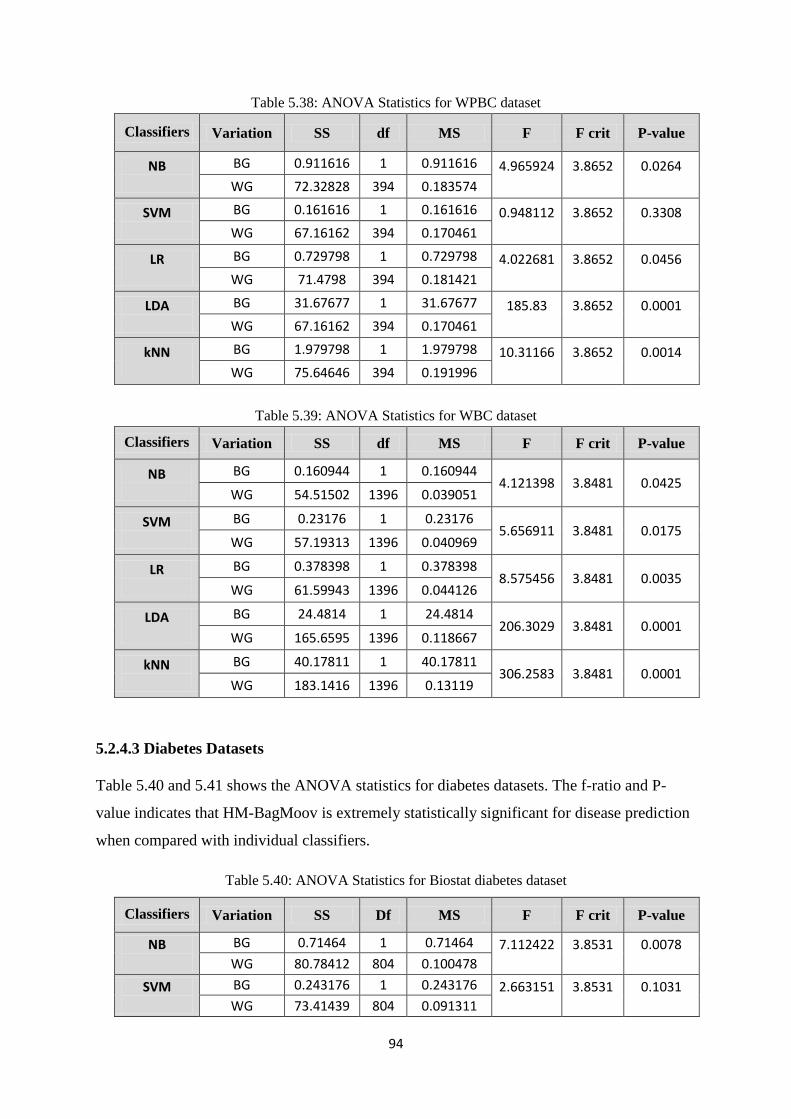
94
Table 5.38: ANOVA Statistics for WPBC dataset
Classifiers Variation SS df MS F F crit P-value
NB
BG 0.911616 1 0.911616 4.965924
3.8652
0.0264 WG 72.32828 394 0.183574
SVM
BG 0.161616 1 0.161616 0.948112
3.8652
0.3308 WG 67.16162 394 0.170461
LR
BG 0.729798 1 0.729798 4.022681
3.8652
0.0456 WG 71.4798 394 0.181421
LDA
BG 31.67677 1 31.67677 185.83
3.8652
0.0001 WG 67.16162 394 0.170461
kNN
BG 1.979798 1 1.979798 10.31166
3.8652
0.0014 WG 75.64646 394 0.191996
Table 5.39: ANOVA Statistics for WBC dataset
Classifiers Variation SS df MS F F crit P-value
NB
BG 0.160944 1 0.160944 4.121398 3.8481 0.0425
WG 54.51502 1396 0.039051
SVM
BG 0.23176 1 0.23176 5.656911 3.8481 0.0175
WG 57.19313 1396 0.040969
LR
BG 0.378398 1 0.378398 8.575456 3.8481 0.0035
WG 61.59943 1396 0.044126
LDA
BG 24.4814 1 24.4814 206.3029 3.8481 0.0001
WG 165.6595 1396 0.118667
kNN
BG 40.17811 1 40.17811 306.2583 3.8481 0.0001
WG 183.1416 1396 0.13119
5.2.4.3 Diabetes Datasets
Table 5.40 and 5.41 shows the ANOVA statistics for diabetes datasets. The f-ratio and P-
value indicates that HM-BagMoov is extremely statistically significant for disease prediction
when compared with individual classifiers.
Table 5.40: ANOVA Statistics for Biostat diabetes dataset
Classifiers Variation SS Df MS F F crit P-value
NB
BG 0.71464 1 0.71464 7.112422
3.8531
0.0078 WG 80.78412 804 0.100478
SVM
BG 0.243176 1 0.243176 2.663151
3.8531
0.1031 WG 73.41439 804 0.091311
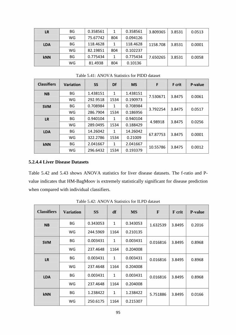
95
LR
BG 0.358561 1 0.358561 3.809365
3.8531
0.0513 WG 75.67742 804 0.094126
LDA
BG 118.4628 1 118.4628 1158.708
3.8531
0.0001 WG 82.19851 804 0.102237
kNN
BG 0.775434 1 0.775434 7.650265
3.8531
0.0058 WG 81.4938 804 0.10136
Table 5.41: ANOVA Statistics for PIDD dataset
Classifiers Variation SS Df MS F F crit P-value
NB
BG 1.438151 1 1.438151 7.530671 3.8475 0.0061
WG 292.9518 1534 0.190973
SVM
BG 0.708984 1 0.708984 3.792254 3.8475 0.0517
WG 286.7904 1534 0.186956
LR
BG 0.940104 1 0.940104 4.98918 3.8475 0.0256
WG 289.0495 1534 0.188429
LDA
BG 14.26042 1 14.26042 67.87753 3.8475 0.0001
WG 322.2786 1534 0.21009
kNN
BG 2.041667 1 2.041667 10.55786 3.8475 0.0012
WG 296.6432 1534 0.193379
5.2.4.4 Liver Disease Datasets
Table 5.42 and 5.43 shows ANOVA statistics for liver disease datasets. The f-ratio and P-
value indicates that HM-BagMoov is extremely statistically significant for disease prediction
when compared with individual classifiers.
Table 5.42: ANOVA Statistics for ILPD dataset
Classifiers Variation SS df MS F F crit P-value
NB
BG 0.343053 1 0.343053 1.632539
3.8495
0.2016 WG 244.5969 1164 0.210135
SVM
BG 0.003431 1 0.003431 0.016816
3.8495
0.8968 WG 237.4648 1164 0.204008
LR
BG 0.003431 1 0.003431 0.016816
3.8495
0.8968 WG 237.4648 1164 0.204008
LDA
BG 0.003431 1 0.003431 0.016816
3.8495
0.8968 WG 237.4648 1164 0.204008
kNN
BG 1.238422 1 1.238422 5.751886
3.8495
0.0166 WG 250.6175 1164 0.215307
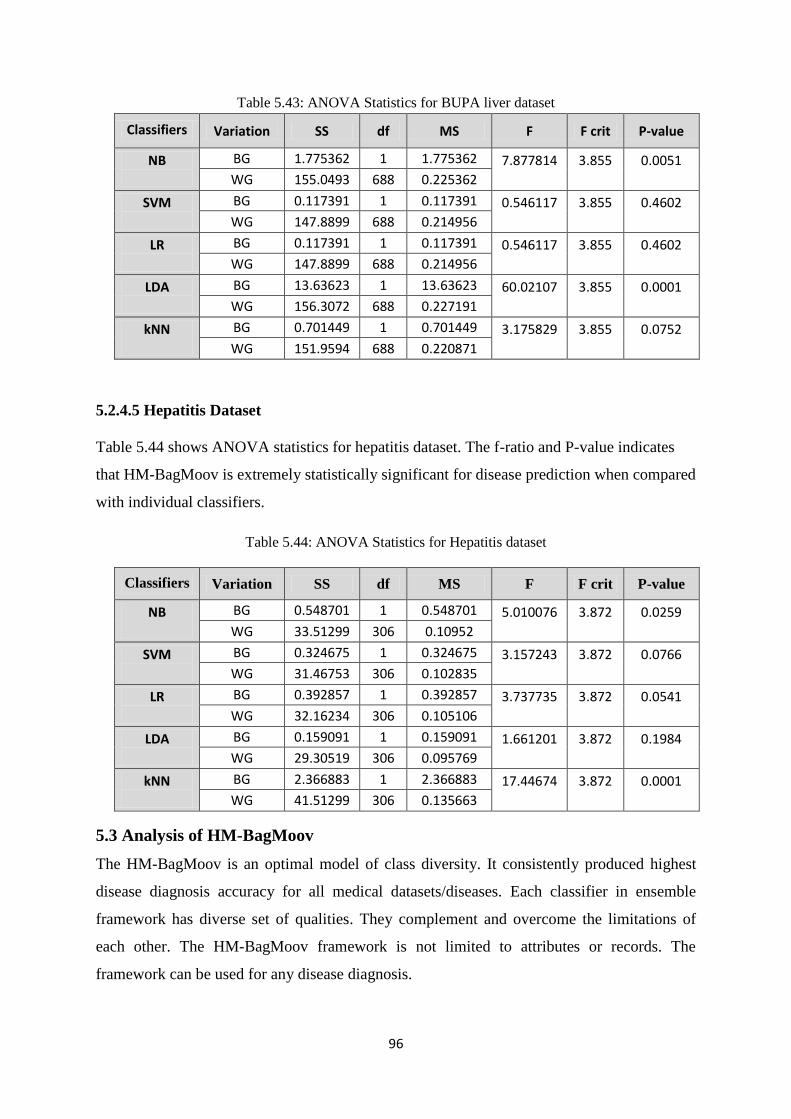
96
Table 5.43: ANOVA Statistics for BUPA liver dataset
Classifiers Variation SS df MS F F crit P-value
NB
BG 1.775362 1 1.775362 7.877814
3.855
0.0051 WG 155.0493 688 0.225362
SVM
BG 0.117391 1 0.117391 0.546117
3.855
0.4602 WG 147.8899 688 0.214956
LR
BG 0.117391 1 0.117391 0.546117
3.855
0.4602 WG 147.8899 688 0.214956
LDA
BG 13.63623 1 13.63623 60.02107
3.855
0.0001 WG 156.3072 688 0.227191
kNN
BG 0.701449 1 0.701449 3.175829
3.855
0.0752 WG 151.9594 688 0.220871
5.2.4.5 Hepatitis Dataset
Table 5.44 shows ANOVA statistics for hepatitis dataset. The f-ratio and P-value indicates
that HM-BagMoov is extremely statistically significant for disease prediction when compared
with individual classifiers.
Table 5.44: ANOVA Statistics for Hepatitis dataset
Classifiers Variation SS df MS F F crit P-value
NB
BG 0.548701 1 0.548701 5.010076
3.872
0.0259 WG 33.51299 306 0.10952
SVM
BG 0.324675 1 0.324675 3.157243
3.872
0.0766 WG 31.46753 306 0.102835
LR
BG 0.392857 1 0.392857 3.737735
3.872
0.0541 WG 32.16234 306 0.105106
LDA
BG 0.159091 1 0.159091 1.661201
3.872
0.1984 WG 29.30519 306 0.095769
kNN
BG 2.366883 1 2.366883 17.44674
3.872
0.0001 WG 41.51299 306 0.135663
5.3 Analysis of HM-BagMoov
The HM-BagMoov is an optimal model of class diversity. It consistently produced highest
disease diagnosis accuracy for all medical datasets/diseases. Each classifier in ensemble
framework has diverse set of qualities. They complement and overcome the limitations of
each other. The HM-BagMoov framework is not limited to attributes or records. The
framework can be used for any disease diagnosis.
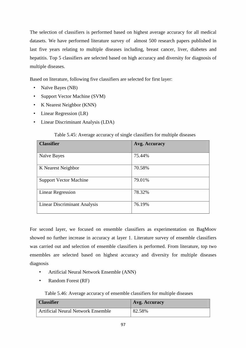
97
The selection of classifiers is performed based on highest average accuracy for all medical
datasets. We have performed literature survey of almost 500 research papers published in
last five years relating to multiple diseases including, breast cancer, liver, diabetes and
hepatitis. Top 5 classifiers are selected based on high accuracy and diversity for diagnosis of
multiple diseases.
Based on literature, following five classifiers are selected for first layer:
• Naïve Bayes (NB)
• Support Vector Machine (SVM)
• K Nearest Neighbor (KNN)
• Linear Regression (LR)
• Linear Discriminant Analysis (LDA)
Table 5.45: Average accuracy of single classifiers for multiple diseases
Classifier Avg. Accuracy
Naïve Bayes 75.44%
K Nearest Neighbor 70.58%
Support Vector Machine 79.01%
Linear Regression 78.32%
Linear Discriminant Analysis 76.19%
For second layer, we focused on ensemble classifiers as experimentation on BagMoov
showed no further increase in accuracy at layer 1. Literature survey of ensemble classifiers
was carried out and selection of ensemble classifiers is performed. From literature, top two
ensembles are selected based on highest accuracy and diversity for multiple diseases
diagnosis
• Artificial Neural Network Ensemble (ANN)
• Random Forest (RF)
Table 5.46: Average accuracy of ensemble classifiers for multiple diseases
Classifier Avg. Accuracy
Artificial Neural Network Ensemble 82.58%

98
Random Forest 83.97%
The HM-BagMoov adopted taxonomy structure which improves classification efficiency and
accuracy. The performance is computed at each level which reduces the risk of making an
error in the top down classification process. HM-BagMoov has different classifiers for
different layers, different features for each layer and classification tasks are more refined. The
layered structure of HM-BagMoov is scalable for hierarchical training and classification.
HM-BagMoov has a novel combination of classifiers using proposed enhanced bagging
ensemble approach for multi-layer framework with high accuracy. In any scenario where one
classifier has some limitation, the other classifier performs well, consequently giving better
performance.
Naïve Bayes classifier considers class conditional independence, therefore loss of accuracy.
Practically, dependencies exist among medical data and this issue is resolved by KNN
classifier which considers similarity between neighbors. Naïve Bayes is efficient in terms of
CPU and memory consumption. It requires very small amount of training data and time.
However, it needs to categorize continuous predictors and this issue is resolved by SVM
which can handle both continuous and categorical attributes well.
K Nearest Neighbor determines similarity between attributes where neighbors determine the
class label for unknown instance which resolves Naïve Bayes issue where each attribute is
considered independently. KNN is very accurate and accuracy degrades with increase of
irrelevant attributes, therefore feature selection is performed to determine subset of relevant
attributes. KNN has simple learning and it is robust to noise.
Support vector machine has high classification and prediction accuracy. It is a good
alternative to neural network. SVM handles both continuous and categorical variables which
resolve Naïve Bayes issue which can handle only categorical variables. SVM decreases the
overfitting issue. However, it is sensitive to noise where pre-processing plays a vital role and
removes noisy data using outlier detection and elimination method.
Artificial neural network has very low prediction error and it is well-suited for continuous-
valued inputs and outputs. It also resolves the Naïve Bayes issue where categorical data is
handled well. ANN is suitable for prediction and disease diagnosis.

99
Random forest improves prediction accuracy compared to single tree. They deal really well
with uneven data sets. RF handles both continuous and nominal attribute. It is fast to build
and faster to predict.
The HM-BagMoov ensemble framework adopted layered approach with enhanced bagging in
order to attain maximum accuracy. The evaluation is performed on multiple benchmark and
real time medical datasets to show the performance. It produced consistent performance for
all medical datasets
5.4 Summary
This chapter presents an experimental evaluation of HM-BagMoov framework for different
medical datasets. Different evaluation metrics are used for results comparison such as
Accuracy, Precision, Recall and F-Measure. The comparison of HM-BagMoov ensemble
with individual classifiers as well as with ensembles and state of the art techniques indicates
that the proposed framework outperformed the rest. Moreover ANOVA is used to show the
significance of our results.
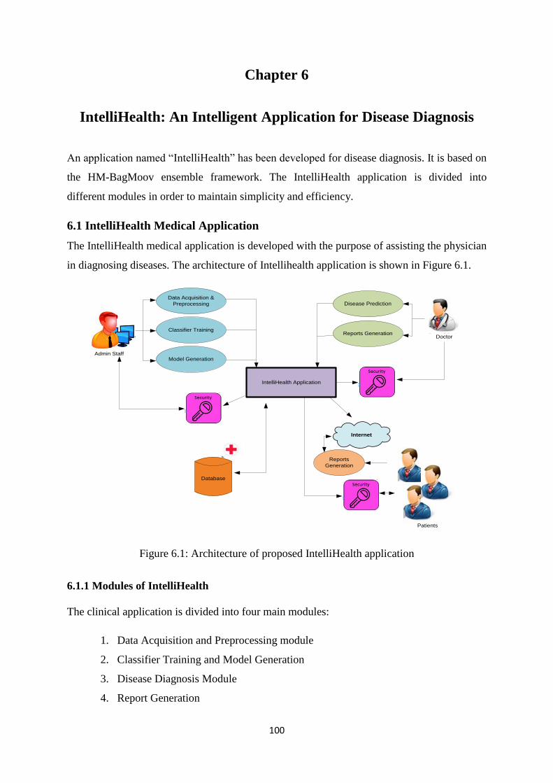
100
Chapter 6
IntelliHealth: An Intelligent Application for Disease Diagnosis
An application named ―IntelliHealth‖ has been developed for disease diagnosis. It is based on
the HM-BagMoov ensemble framework. The IntelliHealth application is divided into
different modules in order to maintain simplicity and efficiency.
6.1 IntelliHealth Medical Application
The IntelliHealth medical application is developed with the purpose of assisting the physician
in diagnosing diseases. The architecture of Intellihealth application is shown in Figure 6.1.
Figure 6.1: Architecture of proposed IntelliHealth application
6.1.1 Modules of IntelliHealth
The clinical application is divided into four main modules:
1. Data Acquisition and Preprocessing module
2. Classifier Training and Model Generation
3. Disease Diagnosis Module
4. Report Generation
IntelliHealth Application
Data Acquisition &
Preprocessing
Classifier Training
Model GenerationAdmin Staff
Internet
DoctorReports Generation
Disease Prediction
Reports
Generation
Patients
Database
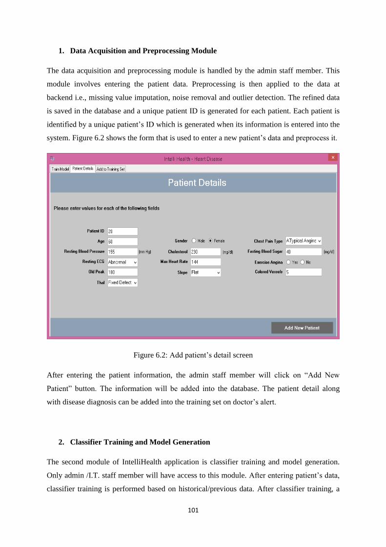
101
1. Data Acquisition and Preprocessing Module
The data acquisition and preprocessing module is handled by the admin staff member. This
module involves entering the patient data. Preprocessing is then applied to the data at
backend i.e., missing value imputation, noise removal and outlier detection. The refined data
is saved in the database and a unique patient ID is generated for each patient. Each patient is
identified by a unique patient‘s ID which is generated when its information is entered into the
system. Figure 6.2 shows the form that is used to enter a new patient‘s data and preprocess it.
Figure 6.2: Add patient‘s detail screen
After entering the patient information, the admin staff member will click on ―Add New
Patient‖ button. The information will be added into the database. The patient detail along
with disease diagnosis can be added into the training set on doctor‘s alert.
2. Classifier Training and Model Generation
The second module of IntelliHealth application is classifier training and model generation.
Only admin /I.T. staff member will have access to this module. After entering patient‘s data,
classifier training is performed based on historical/previous data. After classifier training, a
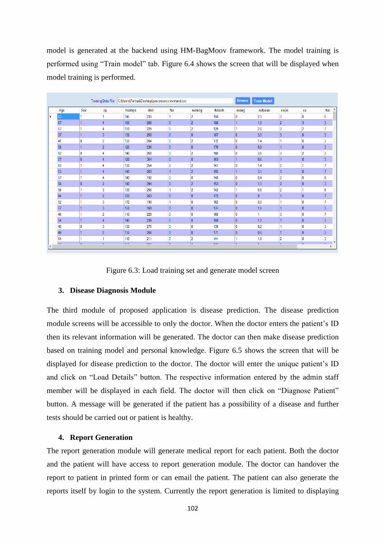
102
model is generated at the backend using HM-BagMoov framework. The model training is
performed using ―Train model‖ tab. Figure 6.4 shows the screen that will be displayed when
model training is performed.
Figure 6.3: Load training set and generate model screen
3. Disease Diagnosis Module
The third module of proposed application is disease prediction. The disease prediction
module screens will be accessible to only the doctor. When the doctor enters the patient‘s ID
then its relevant information will be generated. The doctor can then make disease prediction
based on training model and personal knowledge. Figure 6.5 shows the screen that will be
displayed for disease prediction to the doctor. The doctor will enter the unique patient‘s ID
and click on ―Load Details‖ button. The respective information entered by the admin staff
member will be displayed in each field. The doctor will then click on ―Diagnose Patient‖
button. A message will be generated if the patient has a possibility of a disease and further
tests should be carried out or patient is healthy.
4. Report Generation
The report generation module will generate medical report for each patient. Both the doctor
and the patient will have access to report generation module. The doctor can handover the
report to patient in printed form or can email the patient. The patient can also generate the
reports itself by login to the system. Currently the report generation is limited to displaying
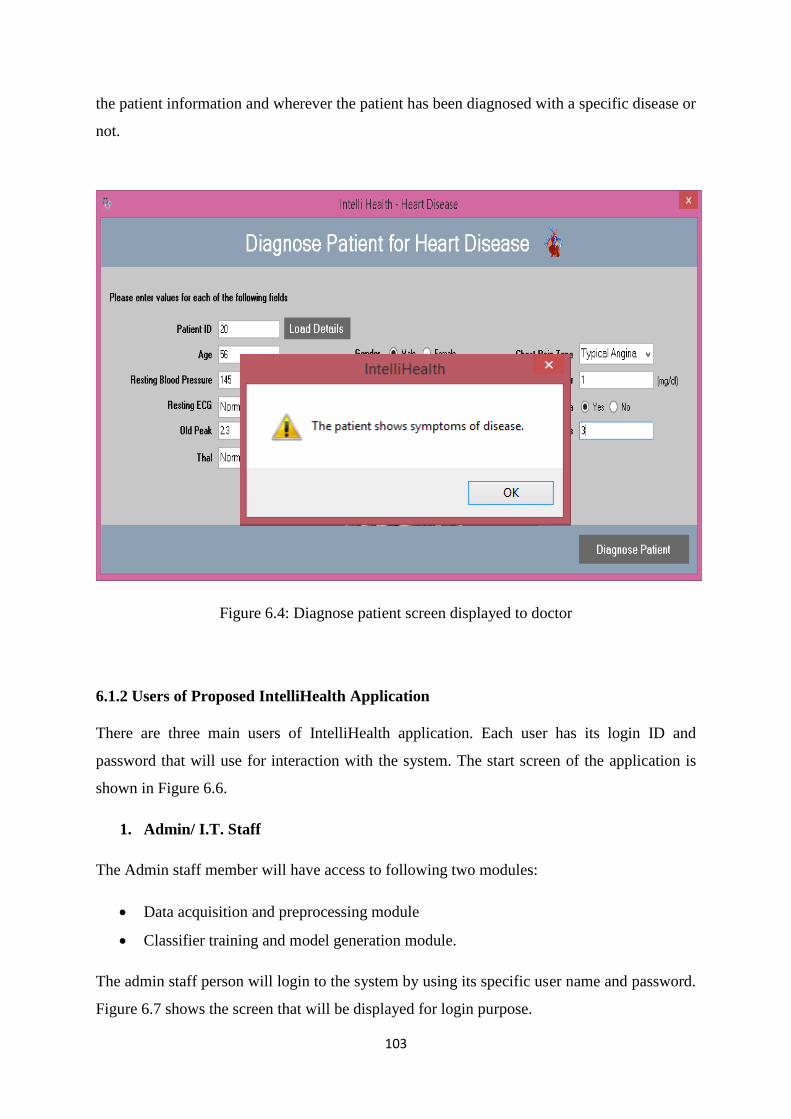
103
the patient information and wherever the patient has been diagnosed with a specific disease or
not.
Figure 6.4: Diagnose patient screen displayed to doctor
6.1.2 Users of Proposed IntelliHealth Application
There are three main users of IntelliHealth application. Each user has its login ID and
password that will use for interaction with the system. The start screen of the application is
shown in Figure 6.6.
1. Admin/ I.T. Staff
The Admin staff member will have access to following two modules:
Data acquisition and preprocessing module
Classifier training and model generation module.
The admin staff person will login to the system by using its specific user name and password.
Figure 6.7 shows the screen that will be displayed for login purpose.

104
Figure 6.5: Start screen of proposed application
Figure 6.6: Login screen of proposed application
After login, the main dashboard of the application will be displayed. The screen shown in
Figure 6.8 will appear when an admin staff member or doctor logs into the system. When
clicked on any icon at dashboard, its related forms will be open.
2. Doctor
Doctor will have access to the following modules:

105
Disease prediction module
Report generation module
After logging in, the main dashboard screen will appear displaying multiple diseases. When
click on any disease, its related modules will be displayed. For disease prediction, the doctor
will enter the patient‘s ID. The information entered will be displayed against that unique ID.
The doctor will then click on ―Diagnosis‖ button for disease prediction. Doctor can then
generate report by clicking on ―Generate Report‖ tab.
Figure 6.7: Dashboard screen of proposed IntelliHealth application
3. Patient
The patient will have access to following module:
Report generation module
The patient will login to the system by entering its specific user name and password. After
login, report generation module will appear. The patient can view its information, its
predicated diagnosis and also can print and email it.
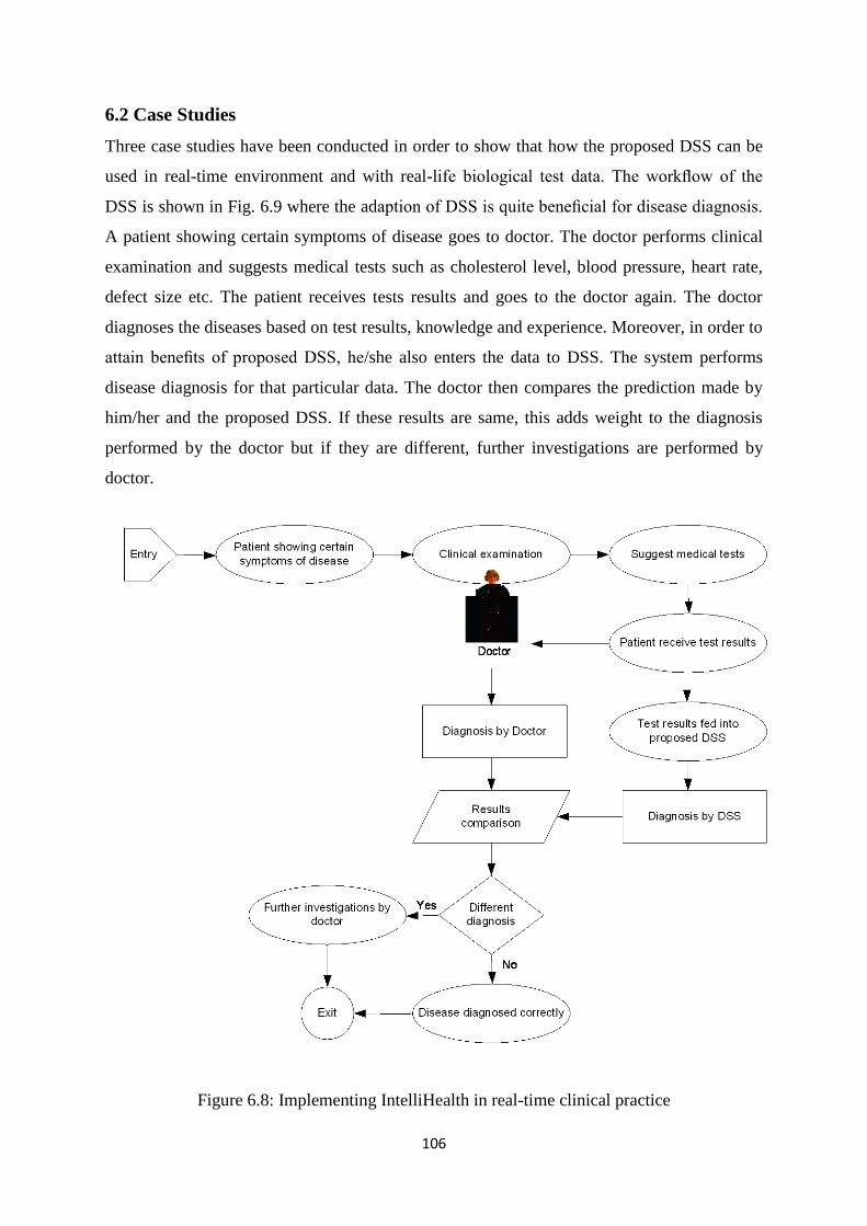
106
6.2 Case Studies
Three case studies have been conducted in order to show that how the proposed DSS can be
used in real-time environment and with real-life biological test data. The workflow of the
DSS is shown in Fig. 6.9 where the adaption of DSS is quite beneficial for disease diagnosis.
A patient showing certain symptoms of disease goes to doctor. The doctor performs clinical
examination and suggests medical tests such as cholesterol level, blood pressure, heart rate,
defect size etc. The patient receives tests results and goes to the doctor again. The doctor
diagnoses the diseases based on test results, knowledge and experience. Moreover, in order to
attain benefits of proposed DSS, he/she also enters the data to DSS. The system performs
disease diagnosis for that particular data. The doctor then compares the prediction made by
him/her and the proposed DSS. If these results are same, this adds weight to the diagnosis
performed by the doctor but if they are different, further investigations are performed by
doctor.
Figure 6.8: Implementing IntelliHealth in real-time clinical practice

107
It should be noted, that an intelligent DSS is not a replacement for doctor or practitioner but it
can help them to gather and interpret information and build a foundation for decision-making
related to particular disease. There are multiple ways in which the proposed DSS can help
both the doctors as well as individual patient. For example
– Diagnose by regularly interpreting and monitoring patient data: The proposed DSS can
implement rules and patterns for individual patients on the basis of clinical parameters and
warning can be generated in case of rule violations.
– Disease management using benchmarks and alerts: A deviation from normal value such as
high heart beat reading could result in an intervention before the condition worsens.
6.2.1 Case Study 1
In order to evaluate the proposed system, collaboration was sought with Rawalpindi Institute
of Cardiology to apply the proposed framework in real-time environment and on real life
data. Rawalpindi Institute of Cardiology is one of the major tertiary cardiac care centers in
Pakistan. This 272-bedded hospital provides care for the cardiac patients from over the
country. It equipped with Coronary Care units, surgical ITC, Departments of Cardiac
Electrophysiology, Echocardiography, Exercise Tolerance Test and Nuclear Cardiology.
They kindly agreed to allow the use of proposed DSS for research purposes only under the
strict supervision of a team of medical experts and their information technology team.
The first step was to build a knowledge from which the classifiers may be trained for
prediction of heart disease. A team of five based on medical practitioners and doctors helped
us to define the medical knowledge in order to classify the healthy and heart disease patients.
A patient will come to the doctor to be diagnosed, the medical knowledge was stated in
natural language and was written as follows: A person is having heart disease if a person has
high blood pressure (BP) of 180/100 and heart rate of 100 beats per minute (BPM), a strong
prior history of cardiovascular ailment, echo results are abnormal and resting
electrocardiographic results are positive then there are strong chances of heart disease. On
the other hand if a person has normal blood pressure (BP) of 120/80 and heart rate of 60
beats per minute (BPM), echo results are normal and no prior history of cardiovascular
disease then there are less chances of heart disease.
In accordance with this knowledge, the features mentioned with the parameters were put in a
dataset along with the diagnosis done by the doctor. All patient names and other identifying
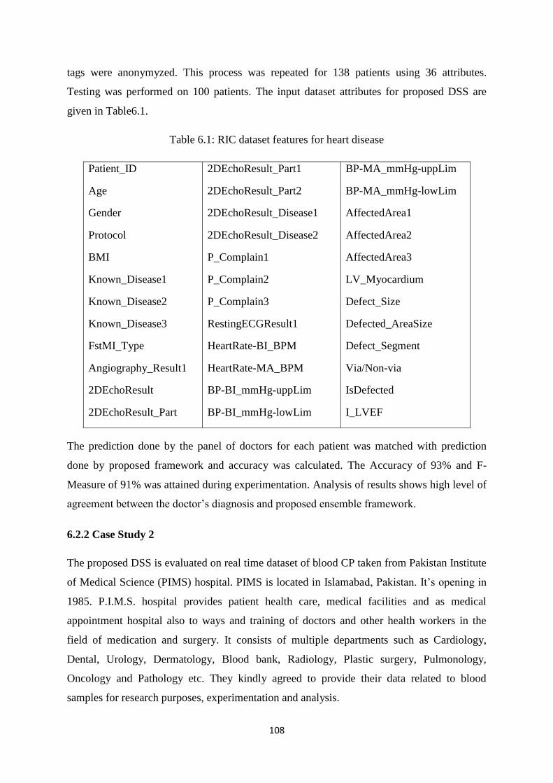
108
tags were anonymyzed. This process was repeated for 138 patients using 36 attributes.
Testing was performed on 100 patients. The input dataset attributes for proposed DSS are
given in Table6.1.
Table 6.1: RIC dataset features for heart disease
Patient_ID
Age
Gender
Protocol
BMI
Known_Disease1
Known_Disease2
Known_Disease3
FstMI_Type
Angiography_Result1
2DEchoResult
2DEchoResult_Part
2DEchoResult_Part1
2DEchoResult_Part2
2DEchoResult_Disease1
2DEchoResult_Disease2
P_Complain1
P_Complain2
P_Complain3
RestingECGResult1
HeartRate-BI_BPM
HeartRate-MA_BPM
BP-BI_mmHg-uppLim
BP-BI_mmHg-lowLim
BP-MA_mmHg-uppLim
BP-MA_mmHg-lowLim
AffectedArea1
AffectedArea2
AffectedArea3
LV_Myocardium
Defect_Size
Defected_AreaSize
Defect_Segment
Via/Non-via
IsDefected
I_LVEF
The prediction done by the panel of doctors for each patient was matched with prediction
done by proposed framework and accuracy was calculated. The Accuracy of 93% and F-
Measure of 91% was attained during experimentation. Analysis of results shows high level of
agreement between the doctor‘s diagnosis and proposed ensemble framework.
6.2.2 Case Study 2
The proposed DSS is evaluated on real time dataset of blood CP taken from Pakistan Institute
of Medical Science (PIMS) hospital. PIMS is located in Islamabad, Pakistan. It‘s opening in
1985. P.I.M.S. hospital provides patient health care, medical facilities and as medical
appointment hospital also to ways and training of doctors and other health workers in the
field of medication and surgery. It consists of multiple departments such as Cardiology,
Dental, Urology, Dermatology, Blood bank, Radiology, Plastic surgery, Pulmonology,
Oncology and Pathology etc. They kindly agreed to provide their data related to blood
samples for research purposes, experimentation and analysis.

109
The IRB approval is required for the datasets when:
Data is accessed through direct intervention or interaction with the individual,
Identifiable private information
There is no direct key or identifier type variable in the blood dataset used in the proposed
research. Moreover the dataset is not private and individually identifiable. Therefore, no IRB
approval is required in order to access and use the blood dataset presented in proposed case
study.
The first step was to build a knowledge from which the classifiers maybe trained for the
prediction of disease. A team of five based on medical practitioners and doctors helped us to
define the medical knowledge in order to classify the healthy and diseased patients. A patient
will come to the doctor to be diagnosed, the medical knowledge was stated in natural
language and was written as follows:
A person is having disease if a person has high T.L.C of 20 unit, platelets count of 80 unit,
hemoglobin of 6 unit and red cell count of 3 unit, then there are strong chances of having any
disease. On the other hand if a person has normal T.L.C of 10 unit, platelets count of 300
unit, hemoglobin of 10 unit and red cell count of 4.8 unit then there are less chances of
disease.
According to the defined knowledge of doctor, the features of blood CP are entered into the
database along with reference values and diagnosis performed by doctor. The personal
information of each patient and other identifying tags are kept anonymyzed for privacy
purposes. We have used 495 patients‘ data consisting of 13 attributes. The evaluation was
performed on 150 patient‘s test set. Following blood CP features are used for real time
evaluation of data.
Table 6.2: PIMS blood CP dataset features for disease prediction
Tests Unit Reference value
T.L.C *1000/µL 4.5-11.5
Red cell count million/µL 3.5-5.5
Haemoglobin g/dL 12-15
PCV/HCT Fl 35-55
MCV Fl 75-100
MCH Pg 25.0-35.0
MCHC g/dL 31.0-38.0
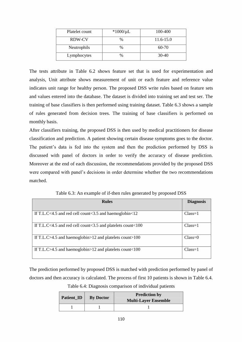
110
Platelet count *1000/µL 100-400
RDW-CV % 11.6-15.0
Neutrophils % 60-70
Lymphocytes % 30-40
The tests attribute in Table 6.2 shows feature set that is used for experimentation and
analysis, Unit attribute shows measurement of unit or each feature and reference value
indicates unit range for healthy person. The proposed DSS write rules based on feature sets
and values entered into the database. The dataset is divided into training set and test ser. The
training of base classifiers is then performed using training dataset. Table 6.3 shows a sample
of rules generated from decision trees. The training of base classifiers is performed on
monthly basis.
After classifiers training, the proposed DSS is then used by medical practitioners for disease
classification and prediction. A patient showing certain disease symptoms goes to the doctor.
The patient‘s data is fed into the system and then the prediction performed by DSS is
discussed with panel of doctors in order to verify the accuracy of disease prediction.
Moreover at the end of each discussion, the recommendations provided by the proposed DSS
were compared with panel‘s decisions in order determine whether the two recommendations
matched.
Table 6.3: An example of if-then rules generated by proposed DSS
Rules Diagnosis
If T.L.C<4.5 and red cell count<3.5 and haemoglobin<12 Class=1
If T.L.C<4.5 and red cell count<3.5 and platelets count<100 Class=1
If T.L.C>4.5 and haemoglobin>12 and platelets count>100 Class=0
If T.L.C>4.5 and haemoglobin>12 and platelets count<100 Class=1
The prediction performed by proposed DSS is matched with prediction performed by panel of
doctors and then accuracy is calculated. The process of first 10 patients is shown in Table 6.4.
Table 6.4: Diagnosis comparison of individual patients
Patient_ID By Doctor Prediction by
Multi-Layer Ensemble
1 1 1

111
2 1 1
3 1 1
4 1 1
5 1 0
6 0 0
7 1 1
8 0 0
9 1 1
10 1 1
The system has achieved 95.19% Accuracy and 93.46% F-Measure for blood CP dataset. It is
clear from the analysis of results that proposed DSS has achieved high classification and
prediction accuracy for a given disease.
6.2.3 Case Study 3
Another case study is in process which is performed by the collaboration with University of
Manchester, UK. The collaboration is done with Dr. Ann Gledson, School of Computer
Science, University of Manchester, UK, Dr. Ben Staller, School of Life Sciences, University
of Manchester, UK and Dr Andrew M Will, Consultant Paediatric Haematologist Central
Manchester University Hospitals, NHS Foundation Trust, Manchester Royal Infirmary, UK.
The evaluation is performed on real-time Haematological cancer dataset. It is one year
collaboration and started on November 2015. The system was train on 2 different types of
Haematological cancers i.e. leukaemias and lymphoma. The model is generated from 5000+
real patients at different level of cancer. The testing is performed on 2000+ patients and
prediction is tracked in real time.
6.3 Summary
In order to facilitate medical practitioner, an application named IntelliHealth is developed
that can assist in disease diagnosis. The application can be used to predict any disease,
however, currently it supports five common diseases i.e., heart disease, breast cancer,
diabetes, liver disease and hepatitis The IntelliHealth application is divided into four main
modules in order to maintain simplicity and efficiency.
112
Chapter 7
Conclusion and Future Work
7.1 Conclusion
Accuracy plays a vital role in the medical field as it concerns with the life of an individual.
Data mining in the medical domain works on the past experiences and analyzes them to
identify the general trends and probable solutions to the present situations. It is an efficient
analytical methodology for detecting unknown and valuable information, from a large
volume of medical data.
In this thesis, we have proposed a clinical decision support framework for disease prediction.
The proposed framework is based on three modules. The first module is data acquisition and
preprocessing which obtains data from different data repositories and preprocess them.
Feature selection, missing value imputation, outlier detection and elimination and noise
removal are performed as preprocessing steps on medical data. Then, the data is divided into
a training set and test set. Each classifier‘s training is performed on the training set in second
module and then they are used to predict unknown class labels for test set instances. The
prediction and evaluation is the third module of the proposed ensemble framework which is
comprised of three classification layers. The proposed HM-BagMoov ensemble uses five
classifiers (NB, LR, LDA, SVM and IBL) at the first layer, then result of these classifiers is
combined using proposed ensemble at second layer and two ensemble classifiers (ANN
ensemble, RF) are added. The result of these three classifiers is again combined using
proposed ensemble approach at the third layer of classification model.
Moreover, an application named IntelliHealth is also developed based on the proposed
ensemble model that can help practitioners and patients for disease prediction based on the
disease symptoms. The IntelliHealth application has four main modules. Module one is used
to enter the medical data from the user and preprocess it. Module two generates the model
using the HM-Bagmoov framework, while the third modules carries out disease prediction.
The last module is used to generate reports.
We have focused on five common diseases, namely, heart disease, breast cancer, diabetes,
liver disease and hepatitis for evaluation of the proposed ensemble method. However, the

113
proposed ensemble can be used to predict any disease. We have used Precision, Recall, F-
Measure and Accuracy to evaluate the performance of our system. The ANOVA statistics, F-
test and P-value are also used for statistical analysis of the proposed system.
Comparison with state of the art techniques also shows the superiority of the proposed
framework. The f-ratio and p-value obtained from ANOVA statistics indicate that the results
are extremely statistically significant for most of the datasets at 95% confidence interval. It is
clear from the analysis of ANOVA statistics that proposed framework results are statistically
significant when compared with other classifiers.
7.2 Future Work
The proposed ensemble model predicts healthy and sick individuals based on their vital signs.
It predicts either class 0 or class 1, representing either absence or presence of a disease.
However, the proposed system can be extended to predict the levels and types of particular
disease such as for heart disease, it can predict different levels of disease like early, acute, etc.
and prediction of type-1 diabetes or prediction of type-2 diabetes in addition of predicting
diabetes.
There are multiple data mining techniques that can be used for disease classification and
prediction into different levels. ID3 and C4.5 are termed as statistical algorithms that are
frequently used for classification of medical datasets.
7.3 Final Word
Decision support is a crucial function for decision makers in many industries. Medical
Decision Support Systems (MDSS) play an increasingly important role in medical practice.
By assisting doctors with making clinical decisions, DSS is expected to improve the quality
of medical care. In this thesis, we presented a novel multi-layer classifier ensemble
framework based on enhanced bagging approach with multi-objective optimized weighted
voting scheme for prediction of multiple diseases. The proposed model named ―HM-
BagMOOV‖ (Hierarchical Multi-level classifiers Bagging with Multi-objective optimized
voting) overcomes the limitations of conventional performance bottlenecks by utilizing an
ensemble of seven heterogeneous classifiers: Naïve Bayes, Linear Regression, Linear
Discriminant Analysis, Instance based Learner, Support Vector Machines, Artificial Neural
Networks and Random Forest. Five different heart disease datasets, four breast cancer
datasets, two diabetes datasets, two liver datasets and one hepatitis dataset are used for

114
experimentation, evaluation and validation. The experimental evaluation shows that the
proposed framework dealt with all types of attributes and achieved high diagnostic accuracy.
Using HM-BagMOOV we have developed a framework and an application both called
―IntelliHealth‖ that may be used by hospitals/doctors for diagnostic advice.
115
References
[1]. Han, J. and Kamber, M.: Data Mining: Concepts and Techniques. Second Edition,
Morgan Kaufmann Publishers, San Francisco (2006)
[2]. R. Kandwal, P. K. Garg and R. D. Garg, Health GIS and HIV/AIDS studies:
Perspective and retrospective, Journal of Biomedical Informatics, vol. 42, pp. 748-
755. (2009)
[3]. Rajkumar A, Reena GS. Diagnosis of heart disease using datamining algorithm.
Global Journal of Computer Science and Technology;10:38-43. (2010)
[4]. Pattekari, S.A.; Parveen, A.: Prediction system for heart disease using Naïve Bayes. .
In: International Journal of Advanced Computer and Mathematical Sciences .Vol 3,
Issue 3, pp 290-294 , (2012).
[5]. Roses, D.F.: Clinical assessment of breast cancer and benign breast disease, Ch. 14.
In: Harris, M.N. (ed.) Breast Cancer, pp. 15–26. Churchill Livingstone, Philadelphia
(2005)
[6]. Kumari, S. and Singh, A.: A Data Mining Approach for the Diagnosis of Diabetes
Mellitus, Proceedings of Seventh lnternational Conference on Intelligent Systems
and Control, pp. 373- 375 (2013)
[7]. Ramana, B.V., Babu, M.S.P., Venkateswarlu, N.B.: A Critical Study of Selected
Classification Algorithms for Liver Disease Diagnosis. International Journal of
Database Management Systems ( IJDMS ), Vol.3, No.2, May (2011)
[8]. Kumar, M. V., Sharathi, V. V., & Devi, B. R. G.: Hepatitis Prediction Model based
on Data Mining Algorithm and Optimal Feature Selection to Improve Predictive
Accuracy. International Journal of Computer Applications, 51(19), 13-16. (2012)
[9]. Third Workshop on Data Mining for Healthcare Management. 16th Pacific-Asia
Conference on Knowledge Discovery and Data Mining. May 29th - Jun 01st - Kuala
Lumpur, Malaysia. (2012)
[10]. https://www.winthrop.org/departments/clinical/cardiology/failure/ [last accessed: 5th
April 2015]
[11]. Subashini, T.S., Ramalingam, V., Palanivel, S.: Breast mass classification based on
cytological patterns using RBFNN and SVM. Expert Syst. Appl. 36, 5284–5290
(2009)
[12]. Vijiyarani, S., Sudha, S.: Disease Prediction in Data Mining Technique – A Survey.
International Journal of Computer Applications & Information Technology, (2013)

116
[13]. Lauritzen, J.N., Arsand, E., Vuurden, K.V., Bellika, J.G., Hejlesen, O.K.,
Hartvigsen, G.: Towards a mobile solution for predicting illness in type 1 diabetes
mellitus In: 2011 2nd International Conference on Wireless Communication,
Vehicular Technology, (2011)
[14]. Rokach, L.: Ensemble-based classifiers. AI Review (2010)
[15]. http://www.soccerpluseducation.org/diabetesmellitus/861/diabetes-medicine-vs-
insulin/ [last accessed: 5th
April 2015]
[16]. Rong-Ho, L.: An intelligent model for liver disease diagnosis. Artificial Intelligence
in Medicine;47:53—62.(2009)
[17]. Lin, R.: An intelligent model for liver disease diagnosis. Artificial Intelligence in
Medicine. Elsevier. Volume 47, Issue 1, Pages 53–62 (2009)
[18]. http://vitaltherapies.com/liver-disease/ [last accessed: 5th
April 2015]
[19]. Nordqvist, C.: What is hepatitis? Symptoms, causes and treatments. Vaterinary
orthopaedics product catalogue. (2015)
[20]. http://www.pnas.org/content/106/31/12986/F1.expansion.html [last accessed: 5th
April 2015]
[21]. Khaleel, M.A., Pradham, S.K., Dash, G.N.: A Survey of Data Mining Techniques on
Medical Data for Finding Locally Frequent Diseases. International Journal of
Advanced Research in Computer Science and Software Engineering. Volume 3,
Issue 8, (2013)
[22]. Chang, C., Wang, C., Jiang, B.C.: Using data mining techniques for multi-diseases
prediction modeling of hypertension and hyperlipidemia by common risk factors.
Expert systems with Applications. Elsevier. Vol 38 issue 5. Pp 5507-5513 (2011)
[23]. Berry, M. J. A., Linoff, G.S.: Mastering Data Mining. New York: Wiley (2000).
[24]. Giudici, P., Applied Data-Mining: Statistical Methods for Business and Industry.
West Sussex, England: John Wiley and Sons (2003).
[25]. Berry, Michael J. A. et al., Data-Mining Techniques for Marketing, Sales and
Customer Support. U.S.A: John Wiley and Sons (1997).
[26]. http://www.md-health.com/Congestive-Heart-Failure.html [last accessed: 5th
April
2015]
[27]. http://medicalterms.info/diseases/Ischemic-Heart-Disease/ [last accessed: 5th
April
2015]
[28]. http://www.nationalbreastcancer.org/types-of-breast-cancer [last accessed: 5th
April
2015]
117
[29]. http://www.medicalnewstoday.com/info/diabetes/diabetessymptoms.php [last
accessed: 5th
April 2015]
[30]. http://www.medicinenet.com/liver_disease/page2.htm [last accessed: 5th
April 2015]
[31]. http://learnaboutcancer.net/liver-cancer/what-causes-liver-cancer.html [last
accessed: 5th
April 2015]
[32]. http://gailssite.weebly.com/alcoholic-liver-disease-ald.html [last accessed: 5th
April
2015]
[33]. http://imgbuddy.com/hepatitis-e-virus-structure.asp [last accessed: 5th
April 2015]
[34]. Sotelsek-Margalef, A., Villena-Román, J.,: MIDAS: An Information-Extraction
Approach to Medical Text Classification. In: Procesamientodellenguaje Natural, pp.
97-104 (2008).
[35]. Palaniappan, S., Awang, R.: Intelligent Heart Disease Prediction System Using Data
Mining Techniques- 978-1-4244-1968-5/08/ 2008 IEEE (2008)
[36]. Naïve Bayes Classifier,
http://en.wikipedia.org/wiki/Naive_Bayes_classifier#cite_note-0 [Accessed: 16
December 2013].
[37]. Rokach, L., Maimon, O.: Decision Trees, Chapter 9. Data mining and knowledge
discovery handbook. Springer. (2010)
[38]. http://mines.humanoriented.com/classes/2010/fall/csci568/portfolio_exports/lguo/dec
isionTree.html [last accessed: 5th
April 2015]
[39]. Shouman, M., Turner, T., Stocker, R.: Using Decision Tree for Diagnosing Heart
Disease Patients, In: Proceedings of the 9th Australasian Data Mining Conference,
Ballarat, Australia (2011).
[40]. Breiman L., Friedman J., Olshen R., and Stone C.: Classification and Regression
Trees. Wadsworth Int. Group, (1984).
[41]. Gelfand S. B., Ravishankar C. S., and Delp E. J., An iterative growing and pruning
algorithm for classification tree design. IEEE Transaction on Pattern Analysis and
Machine Intelligence, 13(2): pp 163-174, (1991).
[42]. Bramer, M.: Principles of data mining. Springer, Berlin (2007)
[43]. Abuhaiba, I.S.I.: Efficient OCR using simple features and decision trees with
backtracking. In: The Arabian Journal for Science and Engineering, Volume
31,(2006).

118
[44]. Jabbar, M.A., Deekshatulu, B.L., Chandra, P.: Classification of heart disease using k
nearest neighbor and genetic algorithm.Procedia Technology Volume 10, pp 85–94.
Elsevier (2013)
[45]. Rafael-Palou, X.: Practical approach to machine learning techniques for
classification and prediction. BDIGITAL (2014)
[46]. Uguroglu, S., Carbonell, J., Doyle , M., Biederman, R.: Cost-Sensitive Risk
Stratification in the diagnosis of Heart Disease.In: Proceedings of the Twenty-Fourth
Innovative Appications of Artificial Intelligence Conference (2012).
[47]. Chitra, R., Seenivasagam, D.V.: Heart Disease Prediction System Using Supervised
Learning Classifier. In: International Journal of Software Engineering and Soft
Computing, Vol. 3, No. 1, March (2013)
[48]. http://yottamine.com/machine-learning-svm [last accessed: 5th
April 2015]
[49]. Wang, S., Mathew, A., Chen, Y., Xi, L., Ma, L., Lee, J.: Empirical Analysis of
Support Vector Machine Ensemble Classifiers. In: Expert Systems with applications,
(2009).
[50]. Mehra, A.: Statistical Sampling and Regression. PreMBA analytical methods (2003)
[51]. http://www.camo.com/rt/Resources/linear_regression_model.html [last accessed: 5th
April 2015]
[52]. Weiss, S.M. and Kulikowski, C.A.: Computer Systems that Learn: Classification
and Prediction Methods from Statistics, Neural Nets, Machine Learning, and Expert
Systems. Morgan Kaufman, (1991).
[53]. Ridella S, Rovetta S, Zunino R.: Circular backpropagation networks for
classification. IEEE Transactions on Neural Networks 8 (1): 84–97 (1997)
[54]. http://scikit-learn.org/0.12/modules/lda_qda.html [last accessed: 5th
April 2015]
[55]. Kruse, R., Borgelt, C., Klawonn, F., Moewes, C.,Steinbrecher, M., Held, P.
Computational Intelligence: A Methodological Introduction. Springer, (2013)
[56]. Ghwanmeh, S., Mohammad, A., Al-Ibrahim, A.: Innovative Artificial Neural
Networks-Based Decision Support System for Heart Diseases Diagnosis. Journal of
Intelligent Learning Systems and Applications, 5, pp 176-183 (2013)
[57]. http://futurehumanevolution.com/artificial-intelligence-future-human-
evolution/artificial-neural-networks [last accessed: 5th
April 2015]
[58]. Das, R., Turkoglu, I., Sengur, A.: Diagnosis of Valvular Heart Disease through
Neural Networks Ensembles, Computer Methods and Programs in Biomedicine,
Vol. 93, No. 2, pp. 185-191. (2009)
119
[59]. Polikar, R.: Ensemble based systems in decision making. IEEE Circuits Syst Mag.
(2006)
[60]. http://cse-wiki.unl.edu/wiki/index.php/Combining_Classifiers [last accessed: 5th
April 2015]
[61]. Moudani, W.: Dynamic Features Selection for Heart Disease Classification. World
Academy of Science, Engineering and Technology Vol:7 (2013)
[62]. Abdullah, A.S. Rajalaxmi, R.R.: A Data mining Model for predicting the Coronary
Heart Disease using Random Forest Classifier. International Conference on Recent
Trends in Computational Methods, Communication and Controls (ICON3C 2012)
[63]. https://citizennet.com/blog/2012/11/10/random-forests-ensembles-and-performance-
metrics/ [last accessed: 5th
April 2015]
[64]. STAT55-Data mining. The Pennsylvania State University.(2014)
[65]. Opitz, D., Maclin, R.: Popular ensemble methods: An empirical study. Journal of
Artificial Intelligence Research 11 (1999) 169-198
[66]. Breiman, L.: Bagging predictors. Mach Learn 24(2):123–140 (2010)
[67]. Maroco, J., Silva, D., Rodrigues, A., Guerreiro, M., Santana, I., Mendonça, A.D.:
Data mining methods in the prediction of Dementia: A real-data comparison of the
accuracy, sensitivity and specificity of linear discriminant analysis, logistic
regression, neural networks, support vector machines, classification trees and
random forests. In: BMC research notes (2011)
[68]. Arnott, D. and Pervan, G.: A critical analysis of decision support systems research,
Journal of Information Technology, 20, 2, 67-87 (2005)
[69]. Bhargava, H. K., Krishnan, R., Müller, R.: Decision Support on Demand: Emerging
Electronic Markets for Decision Technologies,' Decision Support Systems, 19:3, pp.
193-214, 1997.
[70]. http://www.slideshare.net/nijazn/decision-support-system-management-information-
system [last accessed: 5th
April 2015]
[71]. Conejar, R.J., Kim, H.: A Medical Decision Support System (DSS) for Ubiquitous
Healthcare Diagnosis System. International Journal of Software Engineering and Its
Applications Vol. 8, No. 10 pp. 237-244 (2014),
[72]. Anooj, P.K.: Clinical decision support system: Risk level prediction of heart disease
using weighted fuzzy rules. Journal of King Saud University - Computer and
Information Sciences. Volume 24, Issue 1, Pages 27–40 (2012)
120
[73]. Barbosa, J.G.P., Concalves, A.A., Simonetti, V., Leitao, A.R.: A proposed
architecture for implementing a knowledge management system in the Brazilian
National Cancer Institute. Bar-Brazilian administration review. Vol 6 no. 3. Curitiba
Sep (2009)
[74]. Marling, C., Wiley, M., Cooper, T., Bunescu, R., Shubrook, J., Schwartz, F.: The 4
Diabetes Support System: A Case Study in CBR Research and Development. Case-
Based Reasoning Research and Development. Lecture Notes in Computer
Science Volume 6880, pp 137-150 (2011)
[75]. Staes, C.J., Evans, R.S., Rocha, B.H.S.C., Sorensen, J.B., Huff, S.M., Arata, J.,
Narus, S.P.: Computerized Alerts Improve Outpatient Laboratory Monitoring of
Transplant Patients. Journal of American medical informatics association. pp 324-
332. (2008)
[76]. Karthikeyan, T., Thangaraju, P.: Analysis of Classification Algorithms Applied to
Hepatitis Patients. International Journal of Computer Applications (0975 – 8887)
Volume 62– No.15, January (2013)
[77]. Thenmozhi,K.,Deepika, P.: Heart Disease Prediction Using Classification with
Different Decision Tree Techniques. International Journal of Engineering Research
and General Science Volume 2, Issue 6, October-November, 2014
[78]. Chitra, R., Seenivasagam, D.V.: Heart Disease Prediction System Using Supervised
Learning Classifier. In: International Journal of Software Engineering and Soft
Computing, Vol. 3, No. 1, March (2013)
[79]. Shouman,M.,Turner, T., Stocker,R.: Integrating Clustering with Different Data
Mining Techniques in the Diagnosis of Heart Disease. In: Journal of computer
science and engineering, Vol 20, Issue 1, (2013).
[80]. Shouman,M.,Turner, T., Stocker,R.: Integrating Naive Bayes and K-means clustering
with different initial centroid selection methods in the diagnosis of heart disease
patients. In: Computer science and information technology, pp. 125–137, (2012).
[81]. Ghumbre, S., Patil, C., Ghatol, A.: Heart Disease Diagnosis using Support Vector
Machine. In: International Conference on Computer Science and Information
Technology (ICCSIT') Pattaya (2011).
[82]. Shouman, M., Turner, T., Stocker, R.: Using Decision Tree for Diagnosing Heart
Disease Patients, In: Proceedings of the 9th Australasian Data Mining Conference,
Ballarat, Australia (2011).
121
[83]. Chen, A.H., Huang, S.Y., Hong, P.S., Cheng, C.H., Lin, E.J.,: HDPS: Heart Disease
Prediction System. In: Computing in Cardiology, (2011)
[84]. Chaurasia, V., Pal, S.: A Novel Approach for Breast Cancer Detection using Data
Mining Techniques. International Journal of Innovative Research in Computer and
Communication Engineering. Vol. 2, Issue 1, January 2014
[85]. K,A. A., Aljahdali, S., Hussain, S.N.: Comparative Prediction Performance with
Support Vector Machine and Random Forest Classification Techniques.
International Journal of Computer Applications (0975 – 8887) Vol 69– No.11,
(2013).
[86]. Salama, G.I., Abdelhalim, M.B., Zeid, M.A.: Breast Cancer Diagnosis on Three
Different Datasets Using Multi-Classifiers. International Journal of Computer and
Information Technology (2277 – 0764) Vol 01– Issue 01, (2012).
[87]. Lavanya, D., Rani, K.U.: Ensemble decision tree classifier for breast cancer data. In:
International Journal of Information Technology Convergence and Services
(IJITCS) Vol.2. No. 1 (2012).
[88]. Aruna, S., Rajagopalan, S.P., Nandakishore, L.V.: Knowledge based analysis of
various statistical tools in detecting breast cancer. CCSEA, CS & IT, Vol 02, pp. 37–
45 (2011).
[89]. Christobel, A., Sivaprakasam, Y.: An Empirical Comparison of Data Mining
Classification Methods. International Journal of Computer Information Systems,Vol.
3, No. 2, (2011).
[90]. Lavanya, D., Rani,K.U.: Analysis of feature selection with classification: Breast
cancer datasets. Indian Journal of Computer Science and Engineering (IJCSE), Vol
2, No 5 (2011).
[91]. Gandhi, K.K., Prajapati, N.B.: Diabetes prediction using feature selection and
classification. International Journal of Advance Engineering and Research
Development (2014)
[92]. Stahl, F., Johansson, R., Renard, E.: Ensemble Glucose Prediction in Insulin-
Dependent Diabetes. Data driven modeling for diabetes. Springer (2014)
[93]. Aslam, M.W., Zhu, Z., Nandi, A.K.: Feature generation using genetic programming
with comparative partner selection for diabetes classification.In: Expert Systems
with Applications. Elsevier (2013)
122
[94]. NirmalaDevi, M., Appavu, S., Swathi, U.V.: An amalgam KNN to predict diabetes
mellitus. In: International conference on Emerging Trends in Computing,
Communication and Nanotechnology (ICE-CCN), (2013)
[95]. Christobel. Y. A., SivaPrakasam, P.: The Negative Impact of Missing Value
Imputation in Classification of Diabetes Dataset and Solution for Improvement.
IOSR Journal of Computer Engineering (IOSRJCE). Volume 7, Issue 4 (2012), PP
16-23
[96]. Zolfaghari, R.: Diagnosis of Diabetes in Female Population of Pima Indian Heritage
with Ensemble of BP Neural Network and SVM. IJCEM International Journal of
Computational Engineering & Management, Vol. 15 (2012)
[97]. Lee, C.: A Fuzzy Expert System for Diabetes Decision Support Application.
Systems, Man, and Cybernetics, Part B: Cybernetics, IEEE Transactions
on (Volume:41 , Issue: 1 ) PP(139-153) 2011
[98]. Vijayarani, S., Dhayanand, S., Liver Disease Prediction using SVM and Naïve
Bayes Algorithms. International Journal of Science, Engineering and Technology
Research (IJSETR) Volume 4, Issue 4, April 2015
[99]. Jin, H., Kim, S., Kim, J.: Decision Factors on Effective Liver Patient Data
Prediction. International Journal of BioScience and BioTechnology Vol.6, No.4
(2014), pp.167-178
[100]. Sugawara, K., Nakayama, N., Mochida, S.: Acute liver failure in Japan: definition,
classification, and prediction of the outcome. J Gastroenterol. 2012 Aug; 47(8): 849–
861
[101]. Kumar, Y., Sahoo, G.: Prediction of different types of liver diseases using rule based
classification model. Technology and healthcare, vol 21 no. 5, pp 417-432 (2013)
[102]. Ramana, B.V., Babu, M.P.: Liver Classification Using Modified Rotation Forest.
International Journal of Engineering Research and Development. Volume 1, Issue 6.
PP.17-24. (2012)
[103]. Ramana, B.V., Babu, M.P., Venkateswarlu, N.B.: A Critical Study of Selected
Classification Algorithms for Liver Disease Diagnosis. International Journal of
Database Management Systems ( IJDMS ), Vol.3, No.2, (2011)
[104]. Karthik, S., Priyadarishini, A., Anuradha, J., Tripathy, B.K.: Classification and Rule
Extraction using Rough Set for Diagnosis of Liver Disease and its Types. Advances
in Applied Science Research, 2011, 2 (3): 334-345
123
[105]. Pushpalatha, S., Pandya, J.: Data model comparison for Hepatitis diagnosis.
International Journal of Emerging Research in Management &Technology. Volume-
3, Issue-7. Pp 138-141. July 2014
[106]. El Houby, E.M.F.: Analysis of Associative Classification for Prediction of HCV
Response to Treatment. International Journal of Computer Applications (0975 –
8887) Volume 63– No.15, February 2013
[107]. Karthikeyan, T., Thangaraju, P.: Analysis of Classification Algorithms Applied to
Hepatitis Patients. International Journal of Computer Applications (0975 – 8887)
Volume 62– No.15, January (2013)
[108]. Yılmaz Kaya, Murat Uyar, A hybrid decision support system based on rough set and
extreme learning machine for diagnosis of hepatitis disease. 2013 Elsevier, 3429–
3438
[109]. Kumar.M, V., Sharathi.V, V., Devi.B.R.G.: Hepatitis Prediction Model based on
Data Mining Algorithm and Optimal Feature Selection to Improve Predictive
Accuracy. International Journal of Computer Applications (0975 – 8887) Volume
51– No.19, August 2012
[110]. Eldin, A.M.S.A.G.: A Data Mining Approach for the Prediction of Hepatitis C Virus
protease Cleavage Sites. (IJACSA) International Journal of Advanced Computer
Science and Applications, Vol. 2, No. 12, December 2011
[111]. Javad Salimi Sartakht, J. S. (2011). Hepatitis disease diagnosis using a novel hybrid
method. Elsevier, 570-579.
[112]. Yang, J., Lee, Y., Kang, U.: Comparison of Prediction Models for Coronary Heart
Diseases in Depression Patients. International Journal of Multimedia and Ubiquitous
Engineering Vol. 10, No. 3 (2015), pp. 257-268
[113]. Peter, J., Somasundaram.: Probabilistic Classification for Prediction of Heart
Disease. Australian Journal of Basic and Applied Sciences, 9(7), April 2015. Pp
639-643
[114]. Kiruthika, C., Rajini, S.N.S.: An Ill-identified Classification to Predict Cardiac
Disease Using Data Clustering. International Journal of Data Mining Techniques
and Applications. Volume: 03, June 2014, Pages: 321-325
[115]. Sørensen, K.P., Thomassen, M., Tan, Q., Bak, M., Cold, S., Burton, M., Larsen,
M.J., Kruse, T.A.: Long non-coding RNA expression profiles predict metastasis in
lymph node-negative breast cancer independently of traditional prognostic
markers.B reast Cancer Research(2015)
124
[116]. Zand. H.K.K.: A comparitive survey on data mining techniques for breast cancer
diagnosis and prediction. Indian Journal of Fundamental and Applied Life Sciences.
2015 Vol.5 (S1), pp. 4330-4339
[117]. Chaurasia, V., Pal, S.: Data Mining Techniques: To Predict and Resolve Breast
Cancer Survivability. International Journal of Computer Science and Mobile
Computing. Vol.3 Issue.1, January 2014, pg. 10-22
[118]. Chaurasia, V., Pal, S.: A Novel Approach for Breast Cancer Detection using Data
Mining Techniques. International Journal of Innovative Research in Computer and
Communication Engineering. Vol. 2, Issue 1, January 2014
[119]. Kandhasamy, J.P., Balamurali, S.: Performance Analysis of Classifier Models to
Predict Diabetes Mellitus. Procedia Computer Science 47 ( 2015 ) 45 – 51
[120]. Bashir, S., Qamar, U., Khan, F.H.: An efficient rule based classification of diabetes
using ID3, C4.5 and CART ensemble. Frontier Information Technology. IEEE.
Islamabad, Pakistan (2015)
[121]. Gandhi, K.K., Prajapati, N.B.: Diabetes prediction using feature selection and
classification. International Journal of Advance Engineering and Research
Development (2014)
[122]. Tapak, L., Mahjub, H., Hamidi, O., Poorolajal, J., Real-Data Comparison of Data
Mining Methods in Prediction of Diabetes in Iran. Healthcare Information Research.
2013 Sep; 19(3): 177–185.
[123]. Karthikeyani, V., Begum, I.P., Tajudin, K., Begam, I.S.: Comparative of Data
Mining Classification Algorithm (CDMCA) in Diabetes Disease Prediction.
International Journal of Computer Applications (0975 – 8887) Volume 60– No.12,
December 2012
[124]. Julia, A., Vohra, R., Rani, P.: Liver patient classification using intelligent
techniques. International Journal of Computer Science and Information
Technologies, Vol. 5 (4) , 2014, 5110-511
[125]. Sug, H.: Improving the Prediction Accuracy of Liver Disorder Disease with
Oversampling. Applied Mathematics in Electrical and Computer Engineering. Pp
331-335. 2012
[126]. Houby, E.M.F.: A Framework for Prediction of Response to HCV Therapy Using
Different Data Mining Techniques. Advances in Bioinformatics Volume 2014
(2014)

125
[127]. Neshat, M., Sargolzaei, M., Toosi, A.N., Masoumi, A.: Hepatitis Disease Diagnosis
Using Hybrid Case Based Reasoning and Particle Swarm Optimization. Artificial
Intelligence. Volume 2012 (2012), Article ID 609718, 6 pages
[128]. Khan, D.A., Zuhra, F.T., Khan, F.A., Mubarak, A.: Evaluation of diagnostic
accuracy of apri for prediction of fibros is in hepatitis c patients. J Ayub Med Coll
Abbottabad 2008;20(4)

126
APPENDIX
Publications
A.1 Journal Paper
1. Saba Bashir, Farhan Hassan Khan, Usman Qamar, M.Younus Javed ―MV5: A
Clinical Decision Support Framework for Heart Disease Prediction using Majority
Vote based Classifier Ensemble‖ Arabian Journal for Science and Engineering.
Volume 4 Issue 37. Springer, 2014. [Impact Factor: 0.728]
2. Saba Bashir, Usman Qamar, Farhan Hassan Khan ―Heterogeneous Classifiers Fusion
for Dynamic Breast Cancer Diagnosis using Weighted Vote based Ensemble‖ Quality
& Quantity journal, Springer, 2014 [Impact Factor: 0.867]
3. Saba Bashir, Usman Qamar, Farhan Hassan Khan ―BagMOOV: A Novel Ensemble
for Heart Disease Prediction Bootstrap Aggregation with Multi-Objective Optimized
Voting‖ Australasian physical & Engineering sciences in medicine, Springer, 2015
[Impact Factor: 0.676]
4. Saba Bashir, Usman Qamar, Farhan Hassan Khan ―A Multi-Criteria Weighted Vote
based Classifier Ensemble for Heart Disease Prediction‖ Computational Intelligence,
Wiley, 2015 [Impact Factor: 0.722]
5. Saba Bashir, Usman Qamar, Farhan Hassan Khan ―WebMac: A Web based Clinical
Expert System‖ Information Systems Frontier, Springer [Impact Factor: 1.450]
6. Saba Bashir, Usman Qamar, Farhan Hassan Khan ―HMV: A medical decision
support framework using multi-layer classifiers for disease prediction‖ Journal of
Computational Science, Elsevier [Impact Factor: 1.231]
7. Saba Bashir, Usman Qamar, Farhan Hassan Khan ―IntelliHealth: An intelligent
medical decision support system‖, Journal of Biomedical Informatics, Elsevier
[Impact Factor: 2.447]
A.2 International Conference Papers
1. Saba Bashir, Usman Qamar, M.Younus Javed ―An ensemble decision support
framework for intelligent heart disease diagnosis‖ 2014 IEEE International
conference on information society (i-Society), pp. 259-264. London 2014_
2. Saba Bashir, Usman Qamar, M.Younus Javed ―An efficient rule based classification
of diabetes using ID3, C4.5 and CART ensembles‖ 12th IEEE International
Conference on Frontiers of Information Technology (FIT), vol 12. Islamabad 2015


![Intelligent Decision Support Systemsmiquel/idss/IDSS-Part 2-MAI-1112.pdf · Intelligent Decision Support Systems (IDSS) [90s] ... An IEDSS is an intelligent information system that](https://img.pdfslide.net/doc/110x75/5f0913f67e708231d4252044/intelligent-decision-support-systems-miquelidssidss-part-2-mai-1112pdf-intelligent.jpg)