Embed Size (px)
Citation preview

Intention-to-Treat Analysis in Cluster Randomized
Trials with Noncompliance
Booil Jo∗
Department of Psychiatry & Behavioral Sciences
Stanford University
Stanford, CA 94305-5795
Tihomir Asparouhov
Muthen & Muthen
Bengt O. Muthen
Graduate School of Education & Information Studies
University of California, Los Angeles
January 23, 2007
∗The research of the first author was supported by NIMH and NIDA (MH066319, DA11796,MH066247, MH40859). We thank Nick Ialongo for providing the motivating data and for valuableinput. We also thank participants of the Prevention Science Methodology Group for helpful feedback.
1
SUMMARY
In cluster randomized trials (CRT), individuals belonging to the same cluster are
very likely to resemble one another, not only in terms of outcomes, but also in terms of
treatment compliance behavior. Whereas the impact of resemblance in outcomes is well
acknowledged, little attention has been given to the possible impact of resemblance in
compliance behavior. This study defines compliance intraclass correlation as the level
of resemblance in compliance behavior among individuals within clusters, and shows
how compliance intraclass correlation can be a problem in evaluating intention-to-treat
(ITT) effect in CRT. On the basis of Monte Carlo simulations, it is demonstrated that
ignoring compliance information in analyzing data from CRT may result in substantially
decreased power to detect ITT effect, mainly due to compliance intraclass correlation.
As a way of avoiding additional loss of power to detect ITT effect in CRT accompanied
by noncompliance, this study employs an estimation method, where ITT effect estimates
are obtained based on compliance-type-specific treatment effect estimates. A multilevel
mixture analysis using an ML-EM estimation method is used for this estimation.
Key words: cluster randomized trials; noncompliance; intention-to-treat effect; outcome
intraclass correlation; compliance intraclass correlation; multilevel mixture analysis.
2

ITT Analysis in CRT with Noncompliance 3
1 Introduction
In conducting randomized field experiments, individual-level randomization is not al-
ways possible for practical and ethical reasons. Two examples are situations in which a
number of patients belong to each doctor in primary care settings (e.g., [1]), and in school
settings, a number of students belong to each teacher (e.g., [2]). In these situations, it
is problematic (e.g., administrative burden, teacher/parent complaints, ethical reasons)
to assign individuals to different treatment conditions ignoring their cluster member-
ship (i.e., physician, teacher). Therefore, cluster randomized trials (CRT) have been
widely used in practice, treating a cluster of individuals as the unit of randomization.
Although practical/ethical reasons are the main motivation, there is also a statistical
advantage to employing CRT. That is, by assigning individuals that are very likely to
interact to the same treatment condition, each treatment condition is less likely to be
contaminated by other treatment conditions, therefore making the comparison between
different treatment conditions more valid [3]. As a result of cluster-level randomization,
individuals belonging to the same cluster are very likely to resemble one another, not
only in terms of pretreatment characteristics, but also in terms of treatment receipt
behavior and posttreatment outcomes.
If resemblance among individuals is ignored (i.e., data are treated as if they were
from individual-level randomized trials), small variations among individuals within the
same cluster may result in small standard errors, exaggerating the statistical significance
of the effect of treatment assignment, which is a cluster-level variable. An honest (valid)
way of analysis in this situation is to take into account increased variance across clusters
(due to reduced variance within clusters), although it will usually decrease power to
ITT Analysis in CRT with Noncompliance 4
detect treatment assignment effects. For proper analyses accounting for clustered data
structures, multilevel analysis techniques developed in various statistical frameworks can
be employed (e.g., [4-9]). In designing CRT, it is critical to adjust expected statistical
power and required sample sizes assuming that the data will be properly analyzed taking
into account resemblance among individuals with the same cluster membership (e.g.,
[10-11]).
Whereas a good amount of attention has been paid to handling resemblance among
individuals in terms of posttreatment outcomes in CRT, little attention has been given
to handling resemblance among individuals in terms of treatment compliance behavior.
Individuals with the same cluster membership share the environment of the cluster they
belong to, resulting in resemblance among individuals in terms of compliance behavior.
For example, some doctors or teachers, which represent cluster units, may more eagerly
encourage their patients or students to comply with the given treatment. A recent study
[12] called attention to this problem, demonstrating the necessity and possibility of es-
timating compliance-specific treatment assignment effects considering both CRT and
noncompliance. Whereas their study focused on compliance-specific treatment assign-
ment effects (e.g., [13]), the main interest of the current study is in investigating how
resemblance among individuals in compliance behavior influences the intention-to-treat
(ITT) effect and whether the situation can be improved by considering both CRT and
treatment noncompliance in the analysis.
Standard ITT analysis is commonly used in analyzing data from randomized trials
to estimate an overall effect of treatment assignment (i.e., effectiveness) by comparing
groups as randomized. In analyzing data from CRT, the same analysis may be used with
an adjustment for the inflation of type I error, or multilevel analysis techniques can be

ITT Analysis in CRT with Noncompliance 5
employed to estimate ITT effect accounting for resemblance among individuals with the
same cluster membership. Given that we are not interested in compliance-type specific
treatment assignment effects (such as for compliers) and that the effect of cluster-level
randomization can be taken into account in the analysis, it is unclear whether we need
to worry about the effect of treatment noncompliance in estimating ITT effect in CRT.
The current study shows how resemblance in compliance behavior within clusters can
be a problem in evaluating ITT effect in CRT and suggests the use of analyses that
consider both clustering and noncompliance.
2 Motivating Example: JHU PIRC Family-School
Partnership (FSP) Intervention Study
The Johns Hopkins University Preventive Intervention Research Center’s (JHU PIRC)
Family-School Partnership (FSP) intervention trial [2], which was used as a prototype for
the Monte Carlo simulations reported in this study, was designed to improve academic
achievement and to reduce early behavioral problems of school children. First-grade
children were randomly assigned to the intervention or to the control condition, and the
unit of randomization was a classroom (9 classrooms were assigned to the intervention
condition, and another 9 classrooms were assigned to the control condition, with an
average classroom size of 18). Focusing on the shy behavior outcome, the intraclass
correlation was about 0.125 at the 6-month follow-up assessment. It is well known that,
unless properly handled in the analysis, intraclass correlation in posttreatment outcomes
may lead to misestimation of variances, exaggerating statistical significance of treatment
effects in CRT.
ITT Analysis in CRT with Noncompliance 6
In addition to the fact that the unit of randomization was a classroom, another
main complication in the JHU PIRC FSP intervention trial was poor compliance of
parents. In the Family-School Partnership (FSP) intervention condition, parents were
asked to implement 66 take-home activities related to literacy and mathematics. It
was expected that the intervention would not show any desirable effects unless parents
report a quite high level of completion (over-reporting of completion level was very
likely given that parents self-reported). Compliance behavior was observed in the FSP
intervention condition, but not in the control condition, since parents assigned to the
control condition were not invited to implement intervention activities. When the receipt
of intervention is defined as completing at least two thirds of activities, about 46%
of children in the intervention condition properly received the intervention. Further,
parents’ compliance with the intervention activities substantially varied depending on
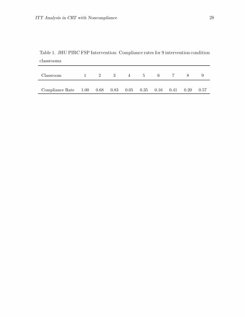
the classroom their children belonged to. Table 1 shows average compliance rates for
the intervention condition classrooms.
[Table 1]
Varying compliance rates across clusters indicate that parents belonging to the same
classroom tend to be similar in terms of compliance behavior (intraclass correlation of
compliance is about 0.377). One possible explanation for this variation would be that,
in some classrooms, teachers (or parents) are more motivated than in other classrooms
(e.g., in Table 1, 100% of parents in one classroom properly implemented the intervention
treatments, whereas in another classroom, 95% of parents did not). The questions here
are whether resemblance in compliance will affect the estimation of ITT effect and
whether standard multilevel analsis techniques can accommodate both complications
(resemblance in both outcomes and compliance) due to cluster-level randomization.
ITT Analysis in CRT with Noncompliance 7
3 Common Setting: CRT with Noncompliance
Let us assume a CRT setting in line with the JHU PIRC FSP interventional trial,
where some study participants do not comply with the given treatment. Individual
i (i = 1, 2, 3,..., mj) belongs to cluster j (j = 1, 2, 3,..., G). The assignment status
Zj denotes the cluster-level randomization status, and Zj = 1 if cluster j is randomly
assigned to the treatment condition, and Zj = 0 if assigned to the control condition.
The observed treatment receipt status Dij = 1 if individual i in cluster j receives
the treatment, and Dij = 0 otherwise. Let Dij(1) denote the potential treatment receipt
status for individual i when Zj = 1, and Dij(0) when Zj = 0. In line with the FSP
intervention trial, it is assumed that study participants were prohibited from receiving
a different treatment than the one that they were assigned to. Therefore, only two
compliance types are possible based on Z and D. The latent compliance type Cij = 1
if individual i would receive the treatment when the treatment is offered, and Cij = 0 if
individual i would not receive the treatment regardless of the intervention assignment.
According to Angrist et al. [13], these two types of individuals are compliers and never-
takers. Since there is only one type of noncomplier (i.e., never-takers), noncomplier will
be used to refer to never-taker. That is,
Cij =
1 (complier) ifDij(1) = 1, and Dij(0) = 0
0 (noncomplier) ifDij(1) = 0, and Dij(0) = 0.
Assuming these two compliance types, a continuous outcome Y for individual i in
cluster j can be expressed as
Yij = αn + (αc − αn)Cij + γc Cij Zj + εbj + εwij, (1)
where αn is the mean potential outcome for noncompliers when Z = 0, αc is the mean

ITT Analysis in CRT with Noncompliance 8
potential outcome for compliers when Z = 0, and αc − αn represents the mean shift
due to compliance. The average effect of treatment assignment for compliers is γc (i.e.,
CACE: complier average causal effect). It is assumed that there is no effect of treatment
assignment for noncompliers, given that noncompliers do not receive the treatment in
either condition. This assumption if often referred to as the exclusion restriction (e.g.,
[13]). The macro-unit residual εbj represents cluster-specific effects given Z, which are
assumed to be normally distributed with zero mean and between-cluster variance σ2b .
The micro-unit residual εwij is assumed to be normally distributed with zero mean and
within-cluster variance σ2w, which is equal across clusters.
In the absence of covariates that predict compliance, the proportions of compliers
and noncompliers can be expressed in the empty logistic regression as
P (Cij = 1) = πij,
P (Cij = 0) = 1 − πij,
logit(πij) = β0 + ξ j . (2)
where πij is the probability of being a complier for individual i in clusterj, and β0 is
the logit intercept. The between-cluster residual ξ j has zero mean and a variance of ψ2b .
The logit value varies across clusters (β0 +ξ j), meaning that the proportion of compliers
differs across clusters. Let πc denote the average compliance rate across all individuals.
3.1 Intraclass Correlations in CRT with Noncompliance
Intraclass correlation (ICC) has been widely used to represent the level of resemblance
among individuals belonging to the same cluster in terms of outcomes. As ICC increases,
variance within clusters will decrease, resulting in inflation of variance across clusters.

ITT Analysis in CRT with Noncompliance 9
The direct consequence of this variance inflation is reduced power to detect the effect of
treatment assignment, which is a cluster-level variable in CRT. However, if this variance
inflation is ignored in the analysis (i.e., data are treated as if they were from individual-
randomized trials), the resulting type I error rate will be incorrectly inflated.
From equation (1), the intraclass correlation coefficient in outcome Y given Z is
defined as
ICCY =σ2
b
σ2b + σ2
w
, (3)
where σ2b denotes the between-cluster variance of outcome Y given Z. The total variance
is the sum of the between- and within-cluster variances (σ2 = σ2b + σ2
w).
In addition to the conventional outcome ICC, another ICC is defined in this study
to represent resemblance among individuals belonging to the same cluster in terms of
compliance behavior. In CRT, individuals belonging to the same cluster are likely to
show resemblance not only in terms of outcomes, but also in terms of compliance be-
havior. The compliance ICC represents a unique complication in CRT accompanied by
treatment noncompliance.
There are several ways to present heterogeneity across clusters in proportions [14-
18]. In line with McKelvey and Zavoina [19], the intraclass correlation coefficient in
compliance can be defined from equation (2) as
ICCC =ψ2
b
ψ2b + π2/3
, (4)
where ψ2b is the between-cluster variance (i.e., variance of ξ j) and π2/3 is the variance
for the within-cluster residual in the logistic distribution. ICCC represents the degree
of resemblance in compliance among individuals belonging to the same cluster. For
example, in the FSP intervention condition in the JHU PIRC trial, the ICCC estimate
ITT Analysis in CRT with Noncompliance 10
is 0.37, which reflects a substantial variation in the average compliance rate across
classrooms.
4 ITT Analysis Considering Clustering
To examine whether ICCC has any impact on the estimation of ITT effect in addition to
ICCY , Monte Carlo simulations are employed in this study, since it is not straightforward
to analytically derive possible bias in variance estimation, given missing compliance
information and mixture distributions of different compliance types.
4.1 Data Generation
The Monte Carlo simulation results presented in this study are based on 500 replications.
The size of each cluster (m) is 20, and the total number of clusters (G) is 100 (50 in
the control and 50 in the treatment condition). Although simulation settings are mostly
based on the JHU PIRC FSP school intervention trial, a larger number of clusters (100
in this study compared to 18 in the JHU Study) is employed to avoid another source
of variance misestimation and to focus on variance misestimation only due to intraclass
correlations. The true ratio of the treatment and control groups is 50%:50% and the
true compliance rate is 50% in all simulation settings.
The true ICCC value ranges from 0.0 to 1.0. A zero ICCC indicates that compliance
behavior is independent of the clusters individuals belong to. A perfect ICCC (i.e., 1.0)
is the other extreme situation, where every individual in the same cluster shows the same
compliance behavior. Although how ICCY affects ITT effect estimation is well known,
two non-zero ICCY values (0.05 and 0.10) were considered in simulations to provide
ITT Analysis in CRT with Noncompliance 11
reference information (i.e., we can tell how much difference ICCC makes in the presence
of ICCY ).
In the setting described in equation (1), compliers and noncompliers may differ in
terms of the outcome mean (i.e., αn and αc) in the control condition. In the standard
ITT analysis, where the distributional distance between compliers and noncompliers is
not taken into account, the distance between the two means simply takes the form of
additional variance in conjunction with variation in compliance (i.e., together with com-
pliance indicator Cij, having a non-zero distance is like having a missing covariate that
predicts Y ). The effect of having this additional variance may be trivial in individually
randomized trials. However, the effect can be substantial in CRT, since the additional
variance may include between-cluster variance (i.e., due to non-zero ICCC). Therefore,
we focus on the distance between the two distributions as a possible source of variance
misestimation in the standard ITT analysis.
Data were generated according to equations (1) and (2). The true within-cluster
variances σ2w takes values of 1.00, 0.95, and 0.90. The true between-cluster variances σ2
b
takes values of 0.00, 0.05, and 0.10 to reflect ICCY of 0.00, 0.05, and 0.10 given the total
variance of 1.0. The true control condition noncomplier mean αn is 1.0, and the true
control condition complier mean αc takes values of 1.0, 1.5, and 2.0 to reflect the distance
between noncompliers and compliers (0.0, 0.5, and 1.0 SD apart). The true treatment
assignment effect for compliers γc (i.e., CACE) is 0.40. The true logit intercept β0 is
zero (i.e., 50% compliance) and the true between-cluster compliance variance ψ2b takes
values of 0.00, 0.82, 2.19, 13.15, and 10000 on the logit scale to reflect ICCC of 0.0, 0.2,
0.4, 0.8 and 1.0 according to equation (4).

ITT Analysis in CRT with Noncompliance 12
4.2 Estimation of ITT Effect Ignoring Noncompliance
In the standard ITT analysis, invidual-level and cluster-level variations in compliance
behavior is not taken into account. Given that, the situation described in equation (1) is
simplified as follows. That is, in this framework, a continuous outcome Y for individual
i in cluster j can be expressed as
Yij = α + γ Zj + εbj + εwij , (5)
where α is the overall mean potential outcome when Z = 0, and the average effect of
treatment assignment is γ (i.e., ITT effect). In relation to parameters in equation (1),
α = αn (1 − πc) + αc πc, where πc is the compliance rate (note that true compliance
rate is 50%). Since true αn = 1.0, and the true αc takes values of 1.0, 1.5, and 2.0,
the true value of α can take values of 1.00, 1.25, and 1.50. In relation to parameters
in equation (1), γ = γc πc. Since the true γc = 0.40 and the true πc = 0.50, the true
value of γ in equation (5) is 0.20. The macro-unit residual εbj is assumed to be normally
distributed with zero mean and between-cluster variance σ2b . The micro-unit residual
εwij is assumed to be normally distributed with zero mean and within-cluster variance
σ2w. If the distance between αn and αc in (1) is not zero, this distance and the variation
in compliance behavior (indicated by Cij) will form a variance that is not accounted for,
distorting the σ2b and σ2
w estimates.
Based on equation (5), two directly estimable population means can be expressed
in terms of model parameters as
µ1 = α + γ , (6)
µ0 = α , (7)
where µ1 is the population mean potential outcome when Z = 1, and µ0 is the population
ITT Analysis in CRT with Noncompliance 13
mean potential outcome when Z = 0.
Then, ITT effect (i.e., γ ) is defined as
ITT = γ = µ1 − µ0 , (8)
where both µ1 and µ0 are directly estimable from the observed data.
Under the condition that individuals are randomly assigned to treatment groups
and that potential outcomes for each person are unrelated to the treatment status of
other individuals (Stable Unit Treatment Value: SUTVA; [20-22]), a large-sample based
single-level estimate of (8) is
ITT = γ = y1 − y0 , (9)
where y1 is the sample mean outcome of the treatment group, and y0 is the sample mean
outcome of the control group.
When dealing with individuals nested within clusters (e.g., students nested within
classrooms, patients nested within doctors) in randomized trials, plausibility of SUTVA
is highly suspected. Cluster-level randomization plays a critical role in making this
obvious violation of SUTVA a more manageable problem by concentrating individuals
who are most likely to interact with one another in the same treatment condition. That
is, in CRT, interaction between individuals assigned to different treatment conditions
is possible, but minimal. For example, in the FSP intervention trial, since the unit
of randomization was a classroom, significant contact or interaction among individuals
assigned to different treatment conditions is unlikely. However, interaction in the same
cluster is highly likely. In the FSP intervention trial, sharing the same teacher and the
same classroom environment is very likely to lead to interaction among individuals in the
same classroom. Whereas interaction across treatment conditions is very hard to handle

ITT Analysis in CRT with Noncompliance 14
(identifying causal effects such as in equation (9) is basically impossible), the interaction
within clusters can be statistically handled. By employing cluster randomization, the
interaction rate among individuals across different treatment conditions remains about
the same as that observed among individuals without systematic nesting structures. In-
teraction within clusters can be handled statistically by considering resemblance among
individuals with the same cluster membership in the analysis, as demonstrated in this
study. For further discussions on SUTVA and CRT, see [3].
Data generated on the basis of equations (1) and (2) are analyzed on the basis of
equation (5), which represents the ITT model considering the fact that randomization
was done at the cluster level, but without considering the fact that some individuals did
not comply with the given treatment. For this analysis, the current study employs a
maximum likelihood estimation approach. The analysis model described in equation (5)
is a standard hierarchical linear model and can be estimated with the ML estimator. A
number of different algorithms are available for obtaining the ML estimates. The most
common are the EM algorithm and the IGLS algorithm, see Raudenbush and Bryk [9].
The ML estimation of the model described in equation (5) has a closed form expression
if all clusters are of equal size however in the general case there is no closed form solution
and the iterative EM or IGLS algorithms are used to obtain the estimates. In this article
we used the EM algorithm [23-24] implemented in Mplus 4.2 [25].
4.3 Impact of Ignoring Noncompliance in ITT Analysis
In ITT analysis ignoring different compliance types, any variance associated with the
compliance type variable Cij may affect the estimation of residual variances in the model.
First, the variance associated with (αc − αn)Cij in equation (1) is not accounted for in

ITT Analysis in CRT with Noncompliance 15
this analysis. Instead, this variance is absorbed by residual variances σ2w and σ2
b (i.e.,
variances σ2w and σ2
b become inflated). Depending on the level of ICCC , the variance
associated with (αc − αn)Cij is differently partitioned into σ2w and σ2
b . For example,
the whole variance associated with (αc − αn)Cij will be added to σ2w if ICCC = 0,
and the whole variance will be added to σ2b if ICCC = 1. If there is no distributional
difference across compliance groups, αc − αn = 0, and therefore the variance associated
with (αc − αn)Cij is zero. In other words, the existence of noncompliance does not
contribute to bias in the estimation of σ2w and σ2
b . Second, there is also a small variance
associated with γc Cij Zj in equation (1), which is not accounted for in the analysis
ignoring different compliance types. As with the variance associated with (αc −αn)Cij,
this variance is also partitioned into σ2w and σ2
b depending on the level of ICCC .
Since the multilevel analysis framework can accommodate inflation of both within-
and between-cluster variances, any variance associated with Cij will be also properly
added to separate residual variances (i.e., within cluster and between cluster). In that
sense, inflated σ2w and σ2
b should not be considered the result of variance misestimation.
Rather, it is the result of correcting for variance that is not accounted for in the model
(i.e., (αc − αn)Cij and γc Cij Zj). Given that, standard errors of the key parameters
in the ITT analysis model (α and γ) can be properly estimated. Simulation results
show 95% confidence interval coverage rates close to 0.95 for these parameter estimates.
However, having extra residual variances can be considered a drawback of ITT analysis
ignoring noncompliance, since it further reduces power to detect an ITT effect (i.e., γ )
in addition to power reduction due to outcome intraclass correlation.
Figure 1 summarizes the ITT analysis results with all simulation settings considered.
It is shown how power decreases as a function of the distributional distance (αc − αn),

ITT Analysis in CRT with Noncompliance 16
compliance intraclass correlation (ICCC), and outcome intraclass correlation (ICCY ).
Power is defined as the proportion of simulation replications out of 500 replications,
in which the treatment effect (γ) estimate is significantly different from zero (at the
conventional significance level of 0.05). Panel (a) in Figure 1 shows how power to detect
ITT effect changes depending on intraclass correlations when compliers and noncompliers
have homogeneous distributions (αc−αn = 0). In general, power shows a trivial change in
this condition as ICCC increases, which is predicted given that the variance associated
with (αc − αn)Cij is zero. A slight decrease in power as a function of ICCC can be
explained by the variance associated with γc Cij Zj , which also inflates σ2w and σ2
b . As
ICCC increases, most of this variance is added to σ2b , resulting in a small but noticeable
decrease in power, especially when ICCY is not zero. Panels (b) and (c) in Figure 1 show
how power changes as complier and noncomplier distributions become farther apart. It
is shown that power decreases substantially as ICCC increases, and that power changes
with a similar pattern under conditions with different outcome intraclass correlations.
The pure impact of ICCC , which can be observed when ICCY = 0, depicts reduction in
power when individuals in the same cluster are similar in terms of compliance behavior,
but not in terms of outcomes. The impact of ICCC alone is quite remarkable, and this
phenomenon has not received enough attention in analyzing data from CRT.
[Figure 1]
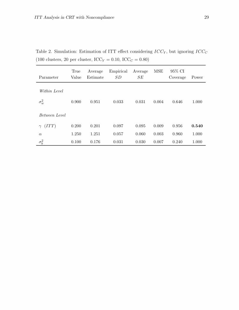
Table 2 shows the detailed results of ITT analysis with one of the simulation settings.
On the basis of equations (1) and (2), the true within-cluster variance σ2w is 0.90 and
the true between-cluster variance σ2b is 0.10 in this setting. Therefore, true ICCY =
0.10 given the total variance of 1.0. The true control condition noncomplier mean αn

ITT Analysis in CRT with Noncompliance 17
is 1.0, and the true control condition complier mean αc is 1.5. The true treatment
assignment effect for compliers γc (i.e., CACE) is 0.40. The true logit intercept β0
is zero (i.e., πc = 0.5), and the true between-cluster compliance variance ψ2b is 13.15,
which corresponds to ICCC of 0.8. The same true values of σ2w and σ2
b are used as
true values for the ITT analysis model, and any deviation from these values can be
attributed to the variance associated with Cij. In the ITT analysis model described in
equation (5), no distinction is made between complier and noncomplier intercepts (or,
the means under the control condition). Therefore, the true overall intercept α = 1.25
(i.e., αn (1−πc)+αc πc = 1.0×(1−0.5)+1.5×0.5 = 1.25). The true value of γ in the ITT
analysis model is calculated as γ = γc πc = 0.4 × 0.5 = 0.2. It is shown in Table 2 that
the true values of parameters α and γ were well recovered in the simulation with good
coverage rates. However, estimates of variances σ2w and σ2
b show substantial deviations
from their true values. The estimated ICCY is now 0.156 (i.e., 0.176/(0.951+0.176)),
which is higher than the true ICCY of 0.100. The estimated power in this simulation
setting is 0.540, which is substantially lower than the typically desired level of power
(i.e., 0.80).
[Table 2]
5 ITT Analysis Considering Both Clustering and
Noncompliance
It is demonstrated in Section 4 how power to detect ITT effect diminishes as ICCC
increases in the analysis where noncompliance is ignored. In Monte Carlo simulations
presented in Section 4, data were generated based on the model described in equations (1)
ITT Analysis in CRT with Noncompliance 18
and (2), but were analyzed based on the model described in equation (5). In this section,
it is examined whether statistical power reduced by not accounting for noncompliance
can be recovered by employing an analysis strategy that considers both clustering and
noncompliance. To reflect heterogeneity between compliers and noncompliers in the data
generation model, the same model described in equations (1) and (2) is used for data
analysis in the simulation study presented in this section.
Based on equations (1) and (2), three directly estimable population means can be
expressed in terms of model parameters as
µ1n = αn, (10)
µ1c = αc + γc, (11)
µ0 = αn (1 − πc) + αc πc, (12)
where πc is the mean proportion of compliers in the population. The population mean
potential outcome when Z = 1 is µ1n for noncompliers and µ1c for compliers. The
population mean potential outcome when Z = 0 is µ0n (i.e., αn) for noncompliers
and µ0c (i.e., αc) for compliers. Under the assumption of the exclusion restriction [13],
the effect of treatment assignment is disallowed for never-takers (i.e., µ1n − µ0n = 0).
Therefore, αn is directly identified as µ1n as shown in equation (10).
Then, from equations (10) and (12), αc is defined as
αc =µ0 − µ1n (1 − πc)
πc, (13)
where µ0, µ1n, and πc are all directly estimable from the observed data.
From equations (11) and (13), γc (CACE) is defined as
γc = µ1c −µ0 − µ1n (1 − πc)
πc, (14)

ITT Analysis in CRT with Noncompliance 19
where µ1c, µ1n, µ0, and πc are directly estimable from the observed data.
Under random assignment of treatment conditions, SUTVA [20-22], and the exclu-
sion restriction, a large-sample based single-level estimate of (14) is
γc = y1c −y0 − y1n (1 − pc)
pc, (15)
where y1c is the sample mean outcome of the treatment group compliers, y1n is the sample
mean outcome of the treatment group noncompliers, y0 is the sample mean outcome
of the control group, and pc is the sample proportion of compliers in the treatment
condition.
Let ITT mix and γmix denote the overall effect of treatment assignment derived
considering the existence of compliers and noncompliers. Under the exclusion restriction,
the effect of treatment assignment for noncompliers is zero. Given that, ITT effect can
be defined based on equation (14) as
ITT mix = γmix = γc πc, (16)
and a large-sample based single-level estimate of (16) is
ITTmix
= γmix = γc pc, (17)
where γc can be identified as in equation (15).
The approximate estimators of γc and ITT mix in equations (15) and (17) reflect the
fact that noncompliance exists, but do not reflect the fact that resemblance (interfer-
ence) among individuals exists in each cluster. In the ML estimation of γc and ITT mix
described below, resemblance among individuals within clusters is accounted for, which
can be seen as a partial relaxation of SUTVA.

ITT Analysis in CRT with Noncompliance 20
Data generated on the basis of the model described in equations (1) and (2) are
analyzed using the same model considering the fact that randomization was done at
the cluster level and that some individuals did not comply with the given treatment.
For this analysis, we employed a formal multilevel mixture analysis [26-27] using the
ML estimator. The observed data likelihood for the treatment and the control group
is different because the compliance variable Cij is observed when Zj = 1 but it is
unobserved when Zj = 0.
In the treatment group the observed data likelihood for cluster j is described as
Lj =∫ (∏
i
f1(Yij | Cij, εbj))φbj(εbj)dεbj ·
∫ (∏
i
πCij
ij (1 − πij)1−Cij
)φj(ξj)dξj , (18)
where f1(Yij | Cij, εbj) is the normal density function
f1(Yij | Cij, εbj) = Exp
(− (Yij − αn − (αc − αn)Cij − γc Cij − εbj)
2
2σ2w
)/(√
2πσw), (19)
φbj(εbj) is the normal density function for εbj
φbj(εbj) = Exp(−ε2bj/(2σ
2b ))/(
√2πσb), (20)
φj(ξj) is the normal density function for ξj
φj(ξj) = Exp(−ξ2j /(2ψ
2))/(√
2πψ), (21)
andπij =
Exp(β0 + ξj)
1 + Exp(β0 + ξj). (22)
In the control group Cij is unobserved and thus the observed data likelihood for
cluster j is
Lj =∫ (∏
i
(f0(Yij | εbj, Cij = 1)πij + f0(Yij | εbj, Cij = 0)(1 − πij)
))φbj(εbj)φj(ξj)dεbjd ξj ,(23)
ITT Analysis in CRT with Noncompliance 21
where f0(Yij | Cij, εbj) is the normal density function
f0(Yij | Cij, εbj) = Exp
(− (Yij − αn − (αc − αn)Cij − εbj)
2
2σ2w
)/(√
2πσw). (24)
The total likelihood function
L =∏
j
Lj (25)
does not have a closed form expression and to compute it we use 2-dimensional numerical
integration. By maximizing L with respect to the parameters in the model we obtain the
ML estimates. The likelihood can be maximized directly by using a general maximization
algorithm. Numerical methods can be used to compute the derivatives of L with respect
to the parameters. A more efficient method for maximizing the likelihood however is
the EM algorithm implemented in Mplus 4.2 [25]. This algorithm treats the unknown
compliance status in the control group as well as the between level random effects as
missing data. Details on the implementation of this algorithm are available in Muthen
and Asparouhov [28]. Parametric standard errors are computed from the information
matrix using the second-order derivatives of L.
Once γc is estimated considering both clustering and noncompliance, ITT effect can
be estimated in the way shown in equation (17). In the simulation results reported in
this study, standard errors of the ITT effect estimates were estimated using the delta
method. That is,
V ar(γcpc) ≈ p2cV ar(γc) + γ2
cV ar(pc) + 2pc γcCov(pc, γc). (26)
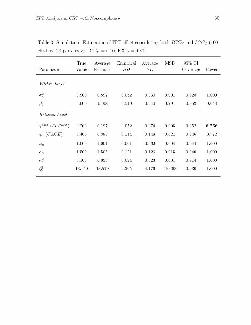
The same set of data analyzed using the ITT analysis considering only clustering,
as reported in Table 2, were reanalyzed considering not only clustering, but also non-
compliance in this section. Table 3 shows the results of this reanalysis. It is shown in

ITT Analysis in CRT with Noncompliance 22
Table 3 that parameters in equations (1) and (2) are well recovered. The γmix (ITTmix)
estimates calculated based on γc (CACE) estimates also show a good coverage rate. The
average standard error (SE) and mean squared error (MSE) of γmix estimates are now
smaller than those of γ estimates shown in Table 2, resulting in higher precision and
accuracy in estimating ITT effect. Consequently, higher power to detect ITT effect is ob-
served when noncompliance is considered in the analysis (i.e., 0.766 in Table 3 compared
to 0.540 in Table 2). Smaller standard errors and higher power to detect ITT effect in
this analysis can be explained by the fact that within- and between-cluster variances (σ2w
and σ2b ) are correctly estimated by simultaneously considering ICCY , ICCC, variances
associated with Cij, and the distance between αc and αn. In the logistic regression of
compliance, the between-cluster variance in compliance ψ2b is correctly estimated, and
therefore the estimated ICCC (i.e., 0.805 = 13.57/(13.57+3.287)) is also close to the true
value of 0.800, which indicates a substantial level of resemblance among individuals with
the same cluster membership in terms of compliance behavior. The estimated ICCY is
now 0.097 (i.e., 0.096/(0.897+0.096)), which is very close to the true ICCY of 0.100.
[Table 3]
The results reported in Tables 2 and 3 show that power to detect ITT effect can
be unnecessarily reduced by not accounting for noncompliance in the model. It is also
shown that the unnecessary loss of power can be recovered by including parameters
related to compliance in the model. A drawback of this approach is that estimation
of γc (CACE), which provides the basis for the estimation of γmix (ITTmix), relies on
untestable identifying assumptions such as the exclusion restriction and monotonicity
[13]. In other words, estimation of ITT effect in CRT is likely to benefit the most from

ITT Analysis in CRT with Noncompliance 23
the analysis based on CACE estimation, if assumptions necessary to identify CACE
are plausible. The assumption of the exclusion restriction is very likely to hold in trials
where successful blinding is possible. In other situations, CACE can be misestimated due
to deviation from the exclusion restriction, which may also bias the estimation of ITT
effect. To alleviate the potential impact of the exclusion restriction violation, estimation
of γc may facilitate auxiliary information such as from proper priors and pretreatment
covariates [12, 29, 30], although these methods are likely to lead to estimation with low
precision. The assumption of monotonicity is likely to hold in trials, where individuals
are more likely to receive the treatment when assigned to the treatment condition than
when assigned to the control condition. For example, in the JHU PIRC FSP interven-
tion study, individuals assigned to the control condition were disallowed to receive the
intervention treatment, and therefore monotonicity is highly likely to hold.
6 Conclusions
Frangakis and Rubin [31] previously pointed out that estimation of intention-to-treat
effect can be biased in the analysis that ignores treatment noncompliance due to in-
teraction between noncompliance and nonresponse (i.e., availability of outcome data at
posttreatment assessments). The current study calls attention to a similar phenomenon
(i.e., how we deal with compliance information in the analysis affects the evaluation
of treatment effects even if we are not interested in estimating compliance-type-specific
treatment assignment effects) in a different context, where noncompliance may interact
with clustering of individuals. It was demonstrated in this study that ignoring com-
pliance information in analyzing data from CRT may result in substantially decreased
ITT Analysis in CRT with Noncompliance 24
power to detect ITT effect, mainly due to compliance intraclass correlation.
As a way of avoiding loss of power to detect ITT effect in CRT accompanied by
noncompliance, this study employed an estimation method, where ITT effect estimates
are obtained on the basis of compliance-type-specific treatment effect estimates. The
same approach was used by Frangakis and Rubin [31] to avoid bias in the estimation of
ITT effect. The limitation of this approach is that ITT effect estimates can be biased if
underlying assumptions employed to identify compliance-type-specific treatment effects
are violated. Given that, although they may seem irrelevant, methods to better handle
identification problems in estimating compliance-type-specific treatment effects are also
likely to improve estimation of ITT effect when faced with various complications in
randomized trials. Extensive treatment of this topic is left for future study.
To simultaneously handle data clustering and noncompliance, this study employed
a formal multilevel analysis combined with the mixture analysis. The joint analysis of
both complications is computationally demanding, but it provides a general framework
that can accommodate various forms of clustered data structures considering mixture
distributions of compliers and noncompliers. The ML-EM estimation of the multilevel
mixture models has been implemented in the Mplus program [25], providing an acces-
sible tool for complex statistical modeling. Although not covered in this study, other
complications in randomized trials such as missing outcomes can also be incorporated
in this estimation framework in addition to noncompliance and data clustering. Further
study is needed for better understanding of how ITT effect estimation may benefit from
the joint modeling of multiple complications in various contexts of randomized trials.

ITT Analysis in CRT with Noncompliance 25
References
1. Dexter P, Wolinsky F, Gramelspacher G, Zhou XH, Eckert G, Waisburd M, Tier-
ney W. Effectiveness of computer-generated reminders for increasing discussions
about Advance Directives and completion of Advance Directives. Annals of Internal
Medicine 1998; 128: 102-110.
2. Ialongo NS, Werthamer L, Kellam SG, Brown CH, Wang S, Lin Y. Proximal impact
of two first-grade preventive interventions on the early risk behaviors for later sub-
stance abuse, depression and antisocial behavior. American Journal of Community
Psychology 1999; 27: 599-642.
3. Sobel ME. What do randomized studies of housing mobility demonstrate: Causal
inference in the face of interference. Journal of the American Statistical Association
2006; 101: 1398-1407.
4. Aitkin M, Longford N. Statistical modeling issues in school effectiveness studies (with
discussion). Journal of Royal Statistical Society, Ser. A 1986; 149: 1-43.
5. Goldstein H. Multilevel mixed linear model analysis using iterative generalized least
squares. Biometrika 1986; 73: 43-56.
6. Liang KH, Zeger SL. Longitudinal data analysis using generalized linear models.
Biometrika 1986; 73: 13-22.
7. McCulloch CE. Maximum likelihood algorithms for generalized linear mixed models.
Journal of the American Statistical Association 1997; 92: 162-170.
8. Muthen BO, Satorra A. Complex sample data in structural equation modeling. In
Sociological Methodology, Marsden PV (ed.). Blackwell: Cambridge, MA, 1995; 267-
316.
9. Raudenbush SW, Bryk AS. Hierarchical Linear Models: Applications and Data Anal-
ysis Methods. Sage: Thousand Oaks, CA, 2002.
10. Donner A, Klar N. Statistical considerations in the design and analysis of community
intervention trials. Journal of Clinical Epidemiology 1996; 49: 435-439.
11. Murray DM. Design and Analysis of Group-Randomized Trials. Oxford University
Press: New York, 1998.

ITT Analysis in CRT with Noncompliance 26
12. Frangakis CE, Rubin DB, Zhou XH. Clustered encouragement design with individ-
ual noncompliance: Bayesian inference and application to advance directive forms.
Biostatistics 2002; 3: 147-164.
13. Angrist JD, Imbens GW, Rubin DB. Identification of causal effects using instrumen-
tal variables. Journal of the American Statistical Association 1996; 91: 444-455.
14. Agresti A. Categorical Data Analysis. Wiley: New York, 1990.
15. Commenges D, Jacqmin H. The intraclass correlation coefficient: distribution-free
definition and test. Biometrics 1994; 50: 517-526.
16. Haldane JBS. The mean and variance of χ2, when used as a test of homogeneity,
when expectations are small. Biometrika 1940; 31: 346-355.
17. McCullagh P, Nelder JA. Generalized Linear Models. Chapman & Hall: London,
1989.
18. Snijders TAB, Bosker RJ. Multilevel Analysis: An Introduction to Basic and Ad-
vanced Multilevel Modeling. Sage: Thousand Oaks, CA, 1999.
19. McKelvey RD, Zavoina W. A statistical model for the analysis of ordinal level
dependent variables. Journal of Mathematical Sociology 1975; 4: 103-120.
20. Rubin DB. Bayesian inference for causal effects: The role of randomization. Annals
of Statistics 1978; 6: 34-58
21. Rubin DB. Discussion of “Randomization analysis of experimental data in the Fisher
randomization test” by D. Basu. Journal of the American Statistical Association
1980; 75: 591-593.
22. Rubin DB. (1990). Comment on “Neyman (1923) and causal inference in experi-
ments and observational studies.” Statistical Science 1990; 5: 472-480.
23. Dempster A, Laird N, Rubin DB. Maximum likelihood from incomplete data via the
EM algorithm. Journal of the Royal Statistical Society, Series B 1977; 39: 1-38.
24. McLachlan GJ, Krishnan T. The EM algorithm and extensions. Wiley: New York,
1997.
25. Muthen LK, Muthen BO. Mplus user’s guide. Muthen & Muthen: Los Angeles,
1998-2006.
ITT Analysis in CRT with Noncompliance 27
26. Asparouhov T, Muthen BO. Multilevel mixture models. In Advances in latent
variable mixture models, Hancock GR and Samuelsen KM (eds.). Information Age
Publishing: Greenwich, CT, 2007.
27. Muthen BO. (2004). Latent variable analysis: Growth mixture modeling and related
techniques for longitudinal data. In Handbook of quantitative methodology for the
social sciences, Kaplan D (ed.). Sage: Newbury Park, CA, 2004; 345-368.
28. Muthen BO, Asparouhov T. Growth mixture analysis: Models with non-Gaussian
random effects. In Advances in Longitudinal Data Analysis, Fitzmaurice G, Davidian
M, Verbeke G, Molenberghs G (eds.). Chapman & Hall: London, 2007.
29. Hirano K, Imbens GW, Rubin DB, Zhou XH. Assessing the Effect of an Influenza
Vaccine in an Encouragement Design. Biostatistics 2000; 1: 69-88.
30. Jo B. Estimating intervention effects with noncompliance: Alternative model speci-
fications. Journal of Educational and Behavioral Statistics 2002; 27: 385-420.
31. Frangakis CE, Rubin DB. Addressing complications of intent-to-treat analysis in the
combined presence of all-or-none treatment-noncompliance and subsequent missing
outcomes. Biometrika 1999; 86: 365-379.
ITT Analysis in CRT with Noncompliance 28
Table 1. JHU PIRC FSP Intervention: Compliance rates for 9 intervention condition
classrooms
Classroom 1 2 3 4 5 6 7 8 9
Compliance Rate 1.00 0.68 0.83 0.05 0.35 0.16 0.41 0.20 0.57
ITT Analysis in CRT with Noncompliance 29
Table 2. Simulation: Estimation of ITT effect considering ICCY , but ignoring ICCC
(100 clusters, 20 per cluster, ICCY = 0.10, ICCC = 0.80)
True Average Empirical Average MSE 95% CIParameter Value Estimate SD SE Coverage Power
Within Level
σ2w 0.900 0.951 0.033 0.031 0.004 0.646 1.000
Between Level
γ (ITT ) 0.200 0.201 0.097 0.095 0.009 0.956 0.540
α 1.250 1.251 0.057 0.060 0.003 0.960 1.000
σ2b 0.100 0.176 0.031 0.030 0.007 0.240 1.000
ITT Analysis in CRT with Noncompliance 30
Table 3. Simulation: Estimation of ITT effect considering both ICCY and ICCC (100
clusters, 20 per cluster, ICCY = 0.10, ICCC = 0.80)
True Average Empirical Average MSE 95% CIParameter Value Estimate SD SE Coverage Power
Within Level
σ2w 0.900 0.897 0.032 0.030 0.001 0.928 1.000
β0 0.000 -0.006 0.540 0.540 0.291 0.952 0.048
Between Level
γ mix (ITT mix) 0.200 0.197 0.072 0.074 0.005 0.952 0.766
γc (CACE) 0.400 0.396 0.144 0.148 0.021 0.946 0.772
αn 1.000 1.001 0.061 0.062 0.004 0.944 1.000
αc 1.500 1.505 0.121 0.126 0.015 0.940 1.000
σ2b 0.100 0.096 0.024 0.023 0.001 0.914 1.000
ζ2b 13.150 13.570 4.305 4.176 18.668 0.930 1.000

ITT Analysis in CRT with Noncompliance 31
0.0 0.2 0.4 0.8 1.0
ICCc
0.2
0.4
0.6
0.8
1.0
Pow
er
(a) 0.0 SD
ICCy=0.00ICCy=0.05ICCy=0.10
0.0 0.2 0.4 0.8 1.0
ICCc
0.2
0.4
0.6
0.8
1.0
(b) 0.5 SD
0.0 0.2 0.4 0.8 1.0
ICCc
0.2
0.4
0.6
0.8
1.0
(c) 1.0 SD
Figure 1: Statistical power to detect ITT effect as a function of ICCC and ICCY
(100 clusters, 20 individuals per cluster). Complier and noncomplier means are (a)
0.0, (b) 0.5, and (c) 1.0 standard deviation apart given treatment assignment.