Embed Size (px)
Citation preview
The Cryosphere, 9, 1797–1817, 2015
www.the-cryosphere.net/9/1797/2015/
doi:10.5194/tc-9-1797-2015
© Author(s) 2015. CC Attribution 3.0 License.
Inter-comparison and evaluation of sea ice algorithms: towards
further identification of challenges and optimal approach using
passive microwave observations
N. Ivanova1, L. T. Pedersen2, R. T. Tonboe2, S. Kern3, G. Heygster4, T. Lavergne5, A. Sørensen5, R. Saldo6,
G. Dybkjær2, L. Brucker7,8, and M. Shokr9
1Nansen Environmental and Remote Sensing Center, Bergen, Norway2Danish Meteorological Institute, Copenhagen, Denmark3University of Hamburg, Hamburg, Germany4University of Bremen, Bremen, Germany5Norwegian Meteorological Institute, Oslo, Norway6Technical University of Denmark, Lyngby, Denmark7NASA Goddard Space Flight Center, Cryospheric Sciences Laboratory, Code 615, Greenbelt, Maryland 20771, USA8Universities Space Research Association, Goddard Earth Sciences Technology and Research Studies and Investigations,
Columbia, Maryland 21044, USA9Environment Canada, Ontario, Canada
Correspondence to: N. Ivanova ([email protected])
Received: 4 February 2015 – Published in The Cryosphere Discuss.: 26 February 2015
Revised: 21 August 2015 – Accepted: 24 August 2015 – Published: 15 September 2015
Abstract. Sea ice concentration has been retrieved in po-
lar regions with satellite microwave radiometers for over
30 years. However, the question remains as to what is an
optimal sea ice concentration retrieval method for climate
monitoring. This paper presents some of the key results of an
extensive algorithm inter-comparison and evaluation experi-
ment. The skills of 30 sea ice algorithms were evaluated sys-
tematically over low and high sea ice concentrations. Evalu-
ation criteria included standard deviation relative to indepen-
dent validation data, performance in the presence of thin ice
and melt ponds, and sensitivity to error sources with seasonal
to inter-annual variations and potential climatic trends, such
as atmospheric water vapour and water-surface roughening
by wind. A selection of 13 algorithms is shown in the article
to demonstrate the results. Based on the findings, a hybrid ap-
proach is suggested to retrieve sea ice concentration globally
for climate monitoring purposes. This approach consists of a
combination of two algorithms plus dynamic tie points im-
plementation and atmospheric correction of input brightness
temperatures. The method minimizes inter-sensor calibration
discrepancies and sensitivity to the mentioned error sources.
1 Introduction
From a perspective of climate change, it is important to know
how fast the total volume of sea ice is changing. In addition to
sea ice thickness (Kern et al., 2015), this requires reliable es-
timates of sea ice concentration (SIC). Consistency in sea ice
climate records is crucial for understanding of internal vari-
ability and external forcing (e.g. Notz and Marotzke, 2012)
in the observed sea ice retreat in the Arctic (Cavalieri and
Parkinson, 2012) and expansion in the Antarctic (Parkinson
and Cavalieri, 2012).
Accuracy and precision serve as measures of performance
of a SIC algorithm. Accuracy (expressed by bias) is the dif-
ference between the mean retrieval and the true value. Pre-
cision (expressed by standard deviation, SD) is the range
within which repeated retrievals of the same quantity scat-
ter around the mean value (see also Brucker et al., 2014,
where precision is addressed in detail). The average accuracy
of commonly known algorithms, such as NASA Team (Cav-
alieri et al., 1984) and Bootstrap (Comiso, 1986), is reported
to be within ± 5 % in winter in a compact (high concentra-
tion) ice pack. The accuracy of the Bootstrap scheme applied
Published by Copernicus Publications on behalf of the European Geosciences Union.
1798 N. Ivanova et al.: Satellite passive microwave measurements of sea ice concentration
to AMSR-E (Advanced Microwave Scanning Radiometer for
Earth Observing System) data, expressed as standard devia-
tion of the scatter around the ice line, was estimated at 2.5 %.
The accuracy including the combined effect of surface tem-
perature and emissivity variability was 4 % (Comiso, 2009).
A comparison of seven algorithms to a trusted data set of
synthetic aperture radar (SAR) and ship-based observations
in the Arctic showed precision of 3–5 %, including sensor
noise (Andersen et al., 2007). In summer and at the ice edge
the retrievals are more uncertain, and accuracy can be as poor
as ± 20 % (Meier and Notz, 2010). Inter-comparison of 11
SIC algorithms in the Arctic showed differences in SIC re-
trievals of 2.0–2.5 % in winter in the areas of consolidated ice
(5–12 % for intermediate SIC) and 2–8 % in summer reach-
ing up to 12 % in the Canadian Archipelago area (Ivanova et
al., 2014). The large uncertainty in retrievals of the summer
period is caused by increased variability in sea ice emissiv-
ity due to the surface wetness and presence of melt ponds.
Part of the uncertainty at low and intermediate SICs, which
is relevant both for summer and for the marginal ice zone at
any time, is caused by atmospheric contributions and wind
roughening of open water areas, as shown for the Arctic
by Andersen et al. (2006). The marginal ice zone is charac-
terised by increased uncertainties due to smearing and foot-
print mismatch effects. The uncertainties over consolidated
ice during Arctic winter were explained by variations in sea
ice emissivity (Andersen et al., 2007).
In this study we focus on the following four error sources,
to which the algorithms have different responses: (1) sensi-
tivity to emissivity and physical temperature of sea ice, (2) at-
mospheric effects, (3) melt ponds, and (4) thin ice. The sen-
sitivity to emissivity and physical temperature of sea ice de-
pends on the selection of input brightness temperatures (Tbs)
available at electromagnetic frequencies between 6 and near
90 GHz in vertical (V) and horizontal (H) polarisations, and
the method applied to retrieve SIC from them, which dis-
tinguishes each algorithm among the others (explained in
Sect. 2.1). Kwok (2002) and Andersen et al. (2007) showed
that SIC algorithms do not reflect the ice concentration vari-
ability in the Arctic adequately when SIC is near 100 %. Vari-
ability due to actual ice concentration changes in the order of
less than 3 % is below the noise floor of the algorithms. Heat
and moisture fluxes between the surface (ocean or ice) and
the atmosphere are sensitive to small variations in the near-
100 % ice cover (Marcq and Weiss, 2012). This unresolved
SIC variability can thus be of significant importance for sea
ice models (and consequently coupled climate models) when
assimilating these data without proper handling of the uncer-
tainties. The apparent fluctuations in the derived ice concen-
tration in the near-100 % ice regime are primarily attributed
to snow/ice surface emissivity variability around the tie point
(predefined Tb for ice) and only secondarily to actual SIC
fluctuations (Andersen et al., 2007).
The second error source is represented by atmospheric ef-
fects, such as water vapour, cloud liquid water (CLW) and
wind roughening of the water surface. It causes the observed
Tb to increase and to change as a function of polarisation and
frequency, season and location (Andersen et al., 2006). This
effect is usually larger during summer and early fall and over
open water (also in the marginal ice zone) because of the
larger amounts of water vapour and CLW in the atmosphere,
and generally more open water areas present.
Algorithms with different sensitivities to surface emissiv-
ity and atmospheric effects produce different estimates of
trends in sea ice area and extent on seasonal and decadal
time scales (Andersen et al., 2007). Effect of diurnal, re-
gional and inter-annual variability of atmospheric forcing on
surface microwave emissivity was also reported in a model
study of Willmes et al. (2014). This means that not only sea
ice area has a climatic trend, but atmospheric and surface
parameters affecting the microwave emission may also have
a trend. Such parameters can be wind patterns, atmospheric
water vapour and CLW (Wentz et al., 2007), snow depth and
snow properties, and the fraction of multi-year ice (MYI).
However, some algorithms are less sensitive than others to
these effects (Andersen et al., 2006; Oelke, 1997), and it is
thus important to select an algorithm with low sensitivity to
them. It is particularly important to have low sensitivity to
error sources which are currently impossible to correct for,
e.g. extinction and emission by CLW or sea ice emissivity
variability. We therefore designed a set of experiments to test
a number of aspects related to SIC algorithm performance,
and ultimately to allow us to select an optimal algorithm for
retrieval of a SIC climate data record.
Melt ponds on Arctic summer sea ice represent an addi-
tional source of errors due to their microwave radiometric
signatures being similar to open water. Virtually all SIC al-
gorithms based on the passive microwave channels around
19, 37, and 90 GHz are very sensitive to presence of melt
water on the ice. The penetration depth of microwave radi-
ation into liquid water is a few millimetres at most (Ulaby
et al., 1986), and therefore it is impossible to distinguish be-
tween ocean water (in leads) and melt water (on the ice). This
is the primary reason why most SIC algorithms are less reli-
able during summer and potentially underestimate the actual
SIC (Fetterer and Untersteiner, 1998; Cavalieri et al., 1990;
Comiso and Kwok, 1996). Melt ponds may exhibit a diurnal
cycle with interchanging periods of open water and thin ice.
This further complicates the SIC retrieval using satellite mi-
crowave radiometry during summer and increases the level
of uncertainty. Some SIC algorithms have been shown to un-
derestimate SIC by up to 40 % in the areas with melt ponds
(Rösel et al., 2012b).
Thin ice is known to be another challenge for the pas-
sive microwave algorithms as they underestimate SIC in such
areas (Heygster et al., 2014; Kwok et al., 2007; Cavalieri,
1994). Recent studies of aerial (Naoki et al., 2008) and satel-
lite (Heygster et al., 2014) passive microwave measurements
show an increase in Tb with sea ice thickness (< 30 cm),
which is more pronounced for lower frequencies and hori-
The Cryosphere, 9, 1797–1817, 2015 www.the-cryosphere.net/9/1797/2015/
N. Ivanova et al.: Satellite passive microwave measurements of sea ice concentration 1799
zontal polarisation. Since an instantaneous amount of thin
ice can reach as much as 1 millionkm2 (total amount glob-
ally, Grenfell et al., 1992), the effect of SIC underestima-
tion can be significant for ice area estimates, air–sea heat and
moisture exchange and modelled ice dynamics. It may also
affect ice volume estimates. It is suggested that the depen-
dency of Tb on the sea ice thickness is due to changes in
near-surface dielectric properties caused, in turn, by changes
of brine salinity with thickness and temperature (Naoki et
al., 2008).
For the first time this many (30) SIC algorithms are
evaluated in a consistent and systematic manner including
both hemispheres, and their performance tested with regard
to high and low SIC, areas with melt ponds, thin ice, at-
mospheric influence and tie points; and covering the ob-
serving characteristics of the Scanning Multichannel Mi-
crowave Radiometer (SMMR), Special Sensor Microwave
Imager (SSM/I) and AMSR-E. The novelty of the presented
approach to algorithm inter-comparison is in the imple-
mentation of all the algorithms with the same tie points,
which helps to avoid subjective tuning, and without applying
weather filters, which have their weaknesses (also addressed
in this study). When evaluating the algorithms, we have fo-
cused in particular on achieving low sensitivity to the error
sources over ice and open water, performance in areas cov-
ered by melt ponds in summer and thin ice in autumn. We
suggest that an optimal algorithm should be adaptable to us-
ing: (1) dynamic tie points in order to reduce inter-instrument
biases and sensitivity to error sources with potential climato-
logical trends and/or seasonal and inter-annual variations and
(2) regional error reduction using meteorological data and
forward models.
The algorithms’ evaluation of algorithms was carried out
in the context of European Space Agency Climate Change
Initiative, Sea Ice (ESA SICCI) and is described in the fol-
lowing sections. Section 2 describes the algorithms and the
basis for selection of the 13 algorithms to be shown in the
following sections. Section 3 describes the data and meth-
ods. Section 4 presents the main results of the work: the
inter-comparison and evaluation of the selected algorithms,
suggested atmospheric correction and dynamic tie points ap-
proach. All the input data and obtained results are collocated
and composed into a reference data set called round robin
data package (RRDP). This is done in order to achieve equal
treatment of all the algorithms during the inter-comparison
and evaluation, as well as to provide an opportunity for fur-
ther tests in a consistent manner. This data set is available
from the Integrated Climate Data Center (ICDC, http://icdc.
zmaw.de/1/projekte/esa-cci-sea-ice-ecv0.html). The discus-
sion and conclusions are provided in Sects. 5 and 6 respec-
tively.
2 The algorithms
During the experiment, we implemented 30 SIC algorithms
and found that they can be grouped according to the selection
of channels and how these are used in each algorithm. We
also found that algorithms within each group had very similar
sensitivity to atmospheric effects and surface emissivity vari-
ations. This is in agreement with sensitivity studies (Tonboe,
2010; Tonboe et al., 2011) using simulated Tbs generated
by combining a thermodynamic ice/snow model to the mi-
crowave emissivity model for layered snow packs (MEMLS)
(Wiesmann and Mätzler, 1999; Tonboe et al., 2006). To avoid
redundancy we only include here a selection of 13 sea ice al-
gorithms (Table 1), which were chosen as representatives of
the groups.
2.1 Selected algorithms
The first group of algorithms, represented by Bootstrap po-
larisation mode (BP, Comiso, 1986), includes polarisation al-
gorithms. These algorithms primarily use 19 or 37 GHz po-
larisation difference (difference between Tbs in vertical and
horizontal polarisations of the same frequency) or polarisa-
tion ratio (polarisation difference divided by the sum of the
two Tbs). The next group uses 19V and 37V channels and
is represented here by CalVal (CV, Ramseier, 1991). Com-
monly known algorithms in this group are NORSEX (Svend-
sen et al., 1983), Bootstrap frequency mode (BF, Comiso,
1986) and UMass-AES (Swift et al., 1985). Bristol (BR,
Smith, 1996) represents the group that uses both polarisa-
tion and spectral gradient information from the channels 19V,
37V and 37H. The NASA Team algorithm (NT, Cavalieri
et al., 1984) uses the polarisation ratio at 19 GHz and the
gradient ratio of 19V and 37V. ASI (The Arctic Radiation
and Turbulence Interaction Study (ARTIST) Sea Ice Algo-
rithm), a non-linear algorithm (Kaleschke et al., 2001), and
Near 90 GHz linear (N90, Ivanova et al., 2013) use the po-
larisation difference at near 90 GHz, both based on Svend-
sen et al. (1987). These are also called near 90 GHz or high-
frequency algorithms. ESMR, named after the single chan-
nel 18H Electrically Scanning Microwave Radiometer on
board Nimbus-5 operating from 1972 to 1977 (e.g. Parkin-
son et al., 2004), and 6H (Pedersen, 1994) are one-channel
algorithms using horizontal polarisation at 18/19 and 6 GHz
respectively. ECICE (Environment Canada’s Ice Concentra-
tion Extractor, Shokr et al., 2008) and NASA Team 2 (NT2,
Markus and Cavalieri, 2000) represent a special class of more
complex algorithms where more channels are used, and ad-
ditional data may be needed as input. Finally we consider
combinations of algorithms (hybrid algorithms), where one
of the algorithms is expected to have low sensitivity to atmo-
spheric effects over open water, and the other is expected to
have a better performance over ice. This group includes the
NT+CV algorithm (Ivanova et al., 2013): an average of NT
and CV, the CV+N90 algorithm (Ivanova et al., 2013): an
www.the-cryosphere.net/9/1797/2015/ The Cryosphere, 9, 1797–1817, 2015
1800 N. Ivanova et al.: Satellite passive microwave measurements of sea ice concentration
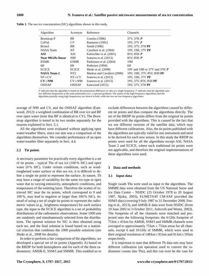
Table 1. The sea ice concentration (SIC) algorithms shown in this study.
Algorithm Acronym Reference Channels
Bootstrap P BP Comiso (1986) 37V, 37H P
CalVal CV Ramseier (1991) 19V, 37V F
Bristol BR Smith (1996) 19V, 37V, 37H PF
NASA Team NT Cavalieri et al. (1984) 19V, 19H, 37V PF
ASI ASI Kaleschke et al. (2001) 85V, 85H P
Near 90GHz linear N90 Ivanova et al. (2013) 85V, 85H P
ESMR ESMR Parkinson et al. (2004) 19H
6H 6H Pedersen (1994) 6H
ECICE ECICE Shokr et al. (2008) 19V and 19H or 37V and 37H P
NASA Team 2 NT2 Markus and Cavalieri (2000) 19V, 19H, 37V, 85V, 85H PF
NT+CV NT+CV Ivanova et al. (2013) 19V, 19H, 37V PF
CV+N90 CV+N90 Ivanova et al. (2013) 19V, 37V, 85V, 85H PF
OSISAF OSISAF Eastwood (2012) 19V, 37V, 37H PF
P indicates that the algorithm is based on the polarisation difference or ratio at a single frequency; F indicates that the algorithm uses
two different frequencies at the same polarisation (i.e., a spectral gradient). The names of the high-frequency algorithms (and the
algorithms partially using high frequencies) are shown in bold, while the rest are low-frequency algorithms.
average of N90 and CV, and the OSISAF algorithm (East-
wood, 2012): a weighted combination of BR over ice and BF
over open water (note that BF is identical to CV). The Boot-
strap algorithm is tested in its two modes separately for the
reasons explained in Sect. 5.1.
All the algorithms were evaluated without applying open
water/weather filters, since our aim was a comparison of the
algorithms themselves. We consider performance of an open
water/weather filter separately in Sect. 4.4.
2.2 Tie points
A necessary parameter for practically every algorithm is a set
of tie points – typical Tbs of sea ice (100 % SIC) and open
water (0 % SIC). Under certain conditions, such as wind-
roughened water surface or thin sea ice, it is difficult to de-
fine a single tie point to represent the surface. In nature, Tb
may have a range of variability for the same ice type or open
water due to varying emissivity, atmospheric conditions, and
temperature of the emitting layer. Therefore the scatter of re-
trieved SIC near the tie points, which correspond to 0 and
100 %, may lead to negative or larger than 100 % SICs. In-
stead of using a set of single tie points to represent the radio-
metric values (e.g., brightness temperature) for each surface
type, the input to the ECICE algorithm is a set of probability
distributions of the radiometric observations. Some 1000 sets
are randomly and simultaneously selected from the distribu-
tions. The optimal solution for SIC is then obtained using
each set, and the final solution is found based on a statisti-
cal criterion that combines the 1000 possible solutions (see
Shokr et al., 2008 for details).
In order to perform a fair comparison of the algorithms, we
developed a special set of tie points (Appendix A) based on
the RRDP for both hemispheres and for each of the three ra-
diometers: AMSR-E, SSM/I and SMMR. This enabled us to
exclude differences between the algorithms caused by differ-
ent tie points and thus compare the algorithms directly. The
set of the RRDP tie points differs from the original tie points
provided with the algorithms. This is caused by the fact that
we use different versions of the satellite data, which may
have different calibrations. Also, the tie points published with
the algorithms are typically valid for one instrument and need
to be derived for each new sensor. In this study the RRDP tie
points were used for all the algorithms except ASI, NASA
Team 2 and ECICE, where such traditional tie points were
not applicable, and therefore the original implementations of
these algorithms were used.
3 Data and methods
3.1 Input data
Single swath Tbs were used as input to the algorithms. The
SMMR data were obtained from the US National Snow and
Ice Data Centre – NSIDC (25 October 1978 to 20 August
1987, Njoku, 2003), EUMETSAT CM-SAF provided the
SSM/I data (covering 9 July 1987 to 31 December 2008, Fen-
nig et al., 2013), and AMSR-E data were from NSIDC (from
19 June 2002 to 3 October 2011; Ashcroft and Wentz, 2003).
The footprints of all the channels were matched and pro-
jected onto the following footprints: the 6 GHz footprint of
75km×43km for AMSR; SSM/I and SMMR channels were
averaged to approximately 75km× 75km areas for all chan-
nels, except 6 and 10 GHz of SMMR, which were used in
their original resolution of 148km×95km and 91km×59km
respectively.
It is important to note that different Tb data sets may have
different calibration (an operation used to convert the ra-
diometer counts into Tbs), and this can even be the case for
The Cryosphere, 9, 1797–1817, 2015 www.the-cryosphere.net/9/1797/2015/
N. Ivanova et al.: Satellite passive microwave measurements of sea ice concentration 1801
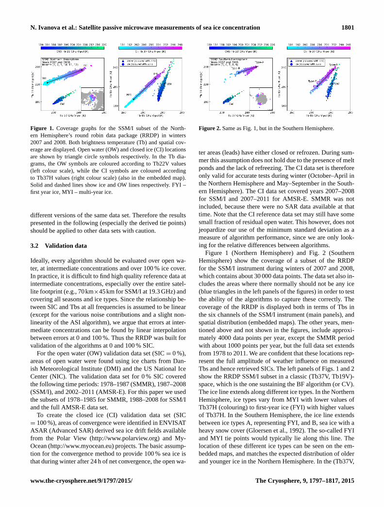
Figure 1. Coverage graphs for the SSM/I subset of the North-
ern Hemisphere’s round robin data package (RRDP) in winters
2007 and 2008. Both brightness temperature (Tb) and spatial cov-
erage are displayed. Open water (OW) and closed ice (CI) locations
are shown by triangle circle symbols respectively. In the Tb dia-
grams, the OW symbols are coloured according to Tb22V values
(left colour scale), while the CI symbols are coloured according
to Tb37H values (right colour scale) (also in the embedded map).
Solid and dashed lines show ice and OW lines respectively. FYI –
first year ice, MYI – multi-year ice.
different versions of the same data set. Therefore the results
presented in the following (especially the derived tie points)
should be applied to other data sets with caution.
3.2 Validation data
Ideally, every algorithm should be evaluated over open wa-
ter, at intermediate concentrations and over 100 % ice cover.
In practice, it is difficult to find high quality reference data at
intermediate concentrations, especially over the entire satel-
lite footprint (e.g., 70km×45km for SSM/I at 19.3 GHz) and
covering all seasons and ice types. Since the relationship be-
tween SIC and Tbs at all frequencies is assumed to be linear
(except for the various noise contributions and a slight non-
linearity of the ASI algorithm), we argue that errors at inter-
mediate concentrations can be found by linear interpolation
between errors at 0 and 100 %. Thus the RRDP was built for
validation of the algorithms at 0 and 100 % SIC.
For the open water (OW) validation data set (SIC = 0 %),
areas of open water were found using ice charts from Dan-
ish Meteorological Institute (DMI) and the US National Ice
Center (NIC). The validation data set for 0 % SIC covered
the following time periods: 1978–1987 (SMMR), 1987–2008
(SSM/I), and 2002–2011 (AMSR-E). For this paper we used
the subsets of 1978–1985 for SMMR, 1988–2008 for SSM/I
and the full AMSR-E data set.
To create the closed ice (CI) validation data set (SIC
= 100 %), areas of convergence were identified in ENVISAT
ASAR (Advanced SAR) derived sea ice drift fields available
from the Polar View (http://www.polarview.org) and My-
Ocean (http://www.myocean.eu) projects. The basic assump-
tion for the convergence method to provide 100 % sea ice is
that during winter after 24 h of net convergence, the open wa-
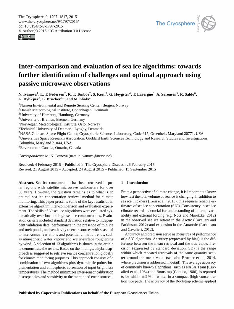
Figure 2. Same as Fig. 1, but in the Southern Hemisphere.
ter areas (leads) have either closed or refrozen. During sum-
mer this assumption does not hold due to the presence of melt
ponds and the lack of refreezing. The CI data set is therefore
only valid for accurate tests during winter (October–April in
the Northern Hemisphere and May–September in the South-
ern Hemisphere). The CI data set covered years 2007–2008
for SSM/I and 2007–2011 for AMSR-E. SMMR was not
included, because there were no SAR data available at that
time. Note that the CI reference data set may still have some
small fraction of residual open water. This however, does not
jeopardize our use of the minimum standard deviation as a
measure of algorithm performance, since we are only look-
ing for the relative differences between algorithms.
Figure 1 (Northern Hemisphere) and Fig. 2 (Southern
Hemisphere) show the coverage of a subset of the RRDP
for the SSM/I instrument during winters of 2007 and 2008,
which contains about 30 000 data points. The data set also in-
cludes the areas where there normally should not be any ice
(blue triangles in the left panels of the figures) in order to test
the ability of the algorithms to capture these correctly. The
coverage of the RRDP is displayed both in terms of Tbs in
the six channels of the SSM/I instrument (main panels), and
spatial distribution (embedded maps). The other years, men-
tioned above and not shown in the figures, include approxi-
mately 4000 data points per year, except the SMMR period
with about 1000 points per year, but the full data set extends
from 1978 to 2011. We are confident that these locations rep-
resent the full amplitude of weather influence on measured
Tbs and hence retrieved SICs. The left panels of Figs. 1 and 2
show the RRDP SSM/I subset in a classic (Tb37V, Tb19V)-
space, which is the one sustaining the BF algorithm (or CV).
The ice line extends along different ice types. In the Northern
Hemisphere, ice types vary from MYI with lower values of
Tb37H (colouring) to first-year ice (FYI) with higher values
of Tb37H. In the Southern Hemisphere, the ice line extends
between ice types A, representing FYI, and B, sea ice with a
heavy snow cover (Gloersen et al., 1992). The so-called FYI
and MYI tie points would typically lie along this line. The
location of these different ice types can be seen on the em-
bedded maps, and matches the expected distribution of older
and younger ice in the Northern Hemisphere. In the (Tb37V,
www.the-cryosphere.net/9/1797/2015/ The Cryosphere, 9, 1797–1817, 2015
1802 N. Ivanova et al.: Satellite passive microwave measurements of sea ice concentration
Tb19V)-space, the OW symbols are grouped mostly in one
point (OW tie point), but also present some spread due to
the noise induced by geophysical parameters such as atmo-
spheric water vapour, liquid water- and ice clouds, surface
temperature variability and surface roughening by wind (all
collectively called geophysical noise). Note that the majority
of the symbols is grouped around one point and a lot less are
spread along the line; however this is not easy to see from the
plots because many points are hidden behind each other. The
Tb22V colouring of the OW symbols illustrates how the vari-
ability of the OW signature is mostly driven by factors im-
pacting also the 22 GHz channel (atmospheric water vapour
content). The length and orientation of the OW spread, and
especially the distance from the OW points to the line of ice
points, determines the strength of algorithms built on these
frequencies (e.g. BF or CV) at low SIC.
The right panels show the same areas but in a (Tb85V,
Tb85H)-space. The ice line is very well defined (limited lat-
eral spread), almost with a slope of one. However, it is dif-
ficult to define an OW point in this axis, since samples are
now spread along a line. This “weather line” even intersects
the ice line, illustrating that algorithms based purely in the
(Tb85V, Tb85H)-space (like the ASI and N90 algorithms)
have difficulties at discriminating open water from sea ice
under certain atmospheric conditions (Kern, 2004).
The embedded maps display the winter location of the
OW samples (same location for the whole RRDP, for
all instruments). In both hemispheres, these locations fol-
low sea ice retreat in summer months to always capture
ocean/atmosphere conditions in the vicinity of sea ice (not
shown). The absence of data near the North Pole is due to
the ENVISAT ASAR not covering areas north of 87◦. The
somewhat limited coverage of the sea ice samples of the Pa-
cific sector in the Northern Hemisphere and many areas in
the Southern Hemisphere is due to scene acquisition strate-
gies of the ENVISAT mission.
After validation of the algorithms using the obtained data
sets at 0 and 100 % we found that some of the algorithms
are hard to validate at these values because they are not de-
signed to enable retrievals outside the SIC range of 0–100 %
(NASA Team2, ECICE) or are affected by a combination of
large bias and nonlinearity at high SIC (ASI). This compli-
cates comparison of these algorithms directly to other algo-
rithms because these effects cut part of the SD of the retrieved
SIC, while we aim at evaluating the full variability around
these reference values (0 and 100 %). We implemented the
algorithms (except these three) without cut-offs, thus allow-
ing SIC values below 0 % and above 100 % as well. In or-
der to be able to include these three algorithms in the inter-
comparison, we have produced reference data sets of Tbs in
every channel that correspond to values of SIC 15 and 75 %
for an additional evaluation. We find that the algorithms’ per-
formance at 15 % is representative of that at 0 %, and so is
75 % representative of 100 %. Therefore we show the results
of evaluation only at SIC 15 and 75 %. By “representative”
here we mean that the algorithms’ ranking does not change
significantly (more details in Sect. 4.1. and Table 2) even
though the absolute values of SD are different.
The SIC 15 % data set was constructed by mixing the av-
erage FYI signature (Tb) with the OW data set, i.e.
Tb15= 0.85 ·Tb(t)+ 0.15 ·Tb100(F̄Y), (1)
where Tb0 (OW Tb) is multiplied by 0.85 (85 % water) and
is varying with time, while Tb100 (ICE Tb) is multiplied by
0.15 (15 % ice) and is an average value of the FYI signa-
ture constant for all data points from the RRDP (see above)
for a given year. By using the SIC 15 % data set we aim at
testing sensitivity of the algorithms to the atmospheric influ-
ence over the ocean and not to variability in emissivity of ice.
Therefore we keep Tb of ice constant.
The SIC 75 % data set was generated similarly to the SIC
15 % data set, but with full variability of ice and 25 % of the
average OW signature:
Tb75= 0.75 ·Tb100(t)+ 0.25 ·Tb0( ¯OW). (2)
For the SIC 75 % data set the variability in Tbs is driven
by variability at SIC 100 % (Tb100(t)), and not at SIC 0 %.
We keep SIC 0 % Tb (Tb0) constant at the average value of
the OW signature for a given year in order to avoid the in-
fluence of seasonally varying atmospheric conditions, which
would have happened if we mixed variable SIC 100 % Tbs
with variable SIC 0 % Tbs. As a consequence, the SIC 75 %
data set will reflect a lower atmospheric variability than we
would have to expect from a real SIC 75 % data set. Since
the CI data set is only valid for the winter season, the same
applies for this SIC 75 % data set.
It is noteworthy that we originally had designed a refer-
ence data set of SIC 85 %, but the positive biases of the ASI
and NASA Team 2 algorithms were larger than 15 % and thus
part of the SD was still cut-off at 100 %. Therefore it was nec-
essary to use a SIC 75 % data set instead. The performance
of the algorithms was consistent between the SIC 75, 85, and
100 % data sets, and therefore we consider such substitution
acceptable. This way of mixing Tbs is not entirely physical
since we are mixing Tbs seen through two different atmo-
spheres. However, since the majority of the signal originates
from either open water or ice, and we use fixed Tbs for the
remaining fraction, we consider the results to be still reason-
ably representative for algorithm performance evaluation.
Normally, SIC products are truncated at 0 and 100 % to al-
low only physically meaningful SIC values, though this does
not apply to ECICE because it employs the inequality con-
straint of 0 % < SIC < 100 % in its optimisation formulation.
However, as the intention here is to investigate the statistical
properties of the retrievals, we will analyse actual SIC as re-
trieved with the algorithms, without truncation, which means
the retrieved values can be negative or above 100 %. Instru-
ment and geophysical noise cause the Tbs to vary around the
chosen tie points, and it cannot be avoided that at least a part
of this noise is translated into some noise in the retrieved SIC.
The Cryosphere, 9, 1797–1817, 2015 www.the-cryosphere.net/9/1797/2015/
N. Ivanova et al.: Satellite passive microwave measurements of sea ice concentration 1803
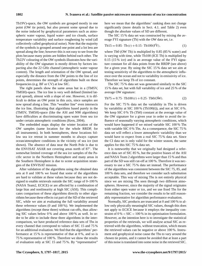
Table 2. (a) Sea ice concentration (SIC) standard deviation (SD) (in %). Low SIC: 15 % (0 % for SMMR), winter (W) and summer (S). No
open water filter applied. Ref – SD for the full SIC 0 % data set. (b) Sea ice concentration (SIC) standard deviation (SD) (in %). High SIC:
75 %, winter. No open water filter applied. Ref – SD for the full SIC 100 % data set.
(a) Northern Hemisphere Southern Hemisphere
AMSR-E SSM/I SMMR AMSR-E SSM/I SMMR
Algorithm Avrg SD S W S W S W Ref Algorithm Avrg SD S W S W S W Ref
6H 2.8 2.0 2.5 – – 2.8 3.8 3.0 6H 2.2 2.1 2.4 – – 1.9 2.2 2.3
CV 3.8 3.6 3.5 4.6 3.8 3.5 3.9 4.8 CV 3.5 3.4 3.4 3.9 4.0 3.0 3.2 3.9
NT+CV 4.5 4.6 4.4 5.1 4.6 3.9 4.2 5.5 NT+CV 3.9 3.9 3.9 4.4 4.5 3.1 3.4 4.4
OSISAF 4.7 5.3 4.8 5.4 4.7 3.8 4.1 5.2 OSISAF 4.3 4.8 4.8 4.9 5.0 3.2 3.4 4.3
NT 5.4 5.8 5.5 5.9 5.5 4.7 4.8 6.6 NT 4.4 4.6 4.6 5.0 5.2 3.4 3.7 5.0
BR 6.6 7.1 6.7 6.6 6.1 6.4 6.4 7.8 BR 6.1 6.7 6.5 6.3 6.2 5.5 5.7 6.9
ESMR 7.2 7.6 7.0 7.9 6.9 7.1 6.5 – NT2 6.2 6.3 6.3 6.2 6.0 – – –
NT2 7.3 6.3 6.7 8.9 7.2 – – – ESMR 6.7 7.3 7.1 6.9 6.9 6.0 6.1 –
ECICE 9.4 10.7 10.0 8.8 8.2 – – – ECICE 9.8 11.1 10.7 8.8 8.5 – – –
BP 13.5 14.5 13.1 12.4 11.4 15.2 14.1 15.5 BP 16.2 17.0 16.2 14.4 14.1 17.6 18.0 17.7
CV+N90 15.8 15.6 15.6 16.5 15.3 – – 19.8 CV+N90 18.9 20.5 19.8 18.0 17.5 – – 22.0
ASI 28.5 31.3 30.1 27.0 25.7 – – – ASI 28.9 32.5 31.1 26.3 25.6 – – –
N90 28.8 28.9 28.8 29.6 27.8 – – 35.9 N90 35.0 38.4 36.9 32.7 32.0 – – 40.8
(b) Northern Hemisphere Southern Hemisphere
Algorithm Avrg SD AMSR-E SSM/I Ref Algorithm Avrg SD AMSR-E SSM/I Ref
BR 3.1 3.1 3.1 4.3 BR 2.9 2.8 3.0 4.5
OSISAF 3.1 3.1 3.1 4.3 OSISAF 2.9 2.8 3.0 4.5
NT+CV 3.1 3.1 3.2 4.4 6H 2.9 2.9 – 4.8
CV+N90 3.4 3.3 3.5 4.6 NT+CV 3.0 2.8 3.1 4.7
NT2 3.7 3.9 3.6 – CV 3.4 3.0 3.7 5.4
6H 3.7 3.7 – 5.4 NT 4.3 4.2 4.4 6.6
NT 3.8 4.0 3.7 5.7 CV+N90 4.6 4.8 4.5 5.9
ASI 3.9 4.7 3.5 – ECICE 4.9 5.4 4.6 –
CV 4.5 4.5 4.5 6.4 ASI 4.9 5.9 4.3 –
BP 4.6 5.2 4.3 6.2 NT2 5.8 5.7 5.8 –
ESMR 4.7 3.0 5.4 – ESMR 7.1 3.9 8.6 –
N90 5.4 5.2 5.5 7.0 N90 8.1 8.4 7.9 10.4
ECICE 8.1 7.4 8.5 – BP 9.0 8.7 9.2 13.1
3.3 Reference data set for melt pond sensitivity
assessment
A daily gridded SIC and melt pond fraction (MPF) refer-
ence data set for the Arctic (Rösel et al., 2012a) was derived
from clear-sky measurements of reflectances in channels 1, 3
and 4 of the MODerate resolution Imaging Spectroradiome-
ter (MODIS) in June–August 2009. The MPF is determined
from classification based on a mixed-pixel approach. It is
assumed that the reflectance measured over each MODIS
500m× 500m grid cell comprises contributions from three
surface types: melt ponds, open water, sea ice/snow (Rösel et
al., 2012a). By using known reflectance values (e.g. Tschudi
et al., 2008) a neural network was built, trained, and applied
(Rösel et al., 2012a). MPF is given as fraction of sea ice
area (not grid cell) covered by melt ponds. For the sensitiv-
ity analysis in this work, a total of 8152 data points were
selected from this data set, so that SD of MPF over each
100km×100km area was less than 5 %, SIC variations were
less than 5 %, SIC itself was larger than 95 % and cloud cover
less than 10 %.
The MODIS data were corrected for bias (Mäkynen et
al., 2014) based on an inter-comparison between ENVISAT
ASAR wide swath mode (WSM) imagery, in situ sea ice
surface observations, weather station reports and the daily
MODIS MPF and SIC data set. It was found that the MODIS
SIC was negatively biased by 3 % and MPF was positively
biased by 8 %. An investigation of the 8-day composite data
set of the MODIS MPF and SIC data set with regard to their
seasonal development during late spring/early summer con-
firmed the existence of such biases.
MODIS SIC was only used for the summer period to eval-
uate the algorithms’ performance over melt ponds, but not
for the SIC validation. This is due to the lack of a sufficiently
quality-controlled MODIS SIC product with potential of a
validation data set. The cloud filters developed for lower lati-
tudes are not reliable enough in the polar latitudes. Moreover,
identification of ice/water in the images depends on thresh-
olds, which will bring the problem of tie points. The vali-
dation of the MPF data set by Rösel et al. (2012a) revealed
accuracy of 5–10 %. Because of the methodology used, the
MPF is tied to the other two surface types: open water in
leads and openings between the ice floes and sea ice/snow.
Therefore it can be assumed that the accuracy of the fraction
of these two other surface types is of the same magnitude as
that of the MPF: 5–10 %, which can be considered as insuf-
ficient for quantitative SIC evaluation.
www.the-cryosphere.net/9/1797/2015/ The Cryosphere, 9, 1797–1817, 2015
1804 N. Ivanova et al.: Satellite passive microwave measurements of sea ice concentration
3.4 Reference data set for the thin ice tests
Sensitivity of the algorithms to thickness of thin (≤ 50 cm)
sea ice was evaluated using a thin ice thickness data set for
the Arctic Ocean, compiled for this particular purpose. To
produce this data set, large (100 km diameter) homogenous
areas of ∼ 100 % thin ice were identified as areas with dark
and homogenous texture by visual inspection of 175 EN-
VISAT ASAR WSM scenes. The same procedure as when
producing ice charts was applied. Thin ice thickness was sub-
sequently derived for these areas using ESA’s L-band Soil
Moisture and Ocean Salinity (SMOS) observations (Hunte-
mann et al., 2014; Heygster et al., 2014). The data set covers
the time period from 1 October to 12 December 2010 and
consists of 991 sea ice thickness data points. For these se-
lected grid cells AMSR-E Tbs were extracted and used as
input to the SIC algorithms.
3.5 Substitution of weather filters by atmospheric
correction
SIC retrievals can be contaminated due to wind roughen-
ing of the ocean surface, atmospheric water vapour and
CLW, as well as precipitation. Traditionally, the atmospheric
effects on the SIC retrievals are removed by applying an
open water/weather filter based on gradient ratios of Tbs for
SMMR (Gloersen and Cavalieri, 1986) and SSM/I (Cavalieri
et al., 1995):
SMMR : SIC= 0 if GR(18/37) > 0.07, (3)
SSM/I : SIC= 0 if GR(19/37) > 0.05
and/or GR(19/22) > 0.045, (4)
where the gradient ratios of Tb18V (Tb19V) and Tb37V
(GR(18/37) and GR(19/37)) are most sensitive to CLW and
the gradient ratio of Tb19V and Tb22V (GR(19/22)) mainly
detects water vapour. We tested the performance of this tech-
nique (more details in Sect. 4.4), and found that it is remov-
ing not only atmospheric effects but also ice itself, which we
found to be unacceptable for a SIC algorithm.
Therefore we chose not to use the open water/weather fil-
ters, but implement an alternative solution, following Ander-
sen et al. (2006) and Kern (2004). The suggested method
consists of applying a more direct atmospheric correction
methodology, where the input SSM/I Tbs in all the channels
used by the algorithms are corrected with regard to atmo-
spheric and surface effects using a radiative transfer model
(RTM):
Tbcorr = Tbmeasured−
(Tbatm−Tbref
), (5)
Tbatm = Tb(f,p,WS,WV,CLW,SST,Tice,SIC,FMYI) , (6)
Tbref = Tb(f,p,0,0,0,SSTref,Tice ref,SIC,FMYI) , (7)
where f is frequency, p is polarisation, WS is wind speed,
WV is water vapour, SST is sea surface temperature, Tice is
ice temperature, and FMYI is MYI fraction (Meissner and
Wentz, 2012; Wentz, 1997). Tbcorr is measured Tb minus
the difference between simulations with (Tbatm) and with-
out (Tbref) atmospheric effects (Meissner and Wentz, 2012;
Wentz, 1997). In order to calculate Tbref, zero values were
assigned to WS, WV and CLW, while SSTref = 271.5 K and
Tice ref = 265 K. 3-hourly fields of 10 m wind speed, total
columnar water vapour, and 2 m air temperature from the
ECMWF ERA-Interim numerical weather prediction (NWP)
re-analysis were used in this process. Following the results of
Andersen et al. (2006) we did not use CLW and precipitation
from the NWP data because these are considered to be less
consistent with the observed Tbs (also confirmed by our own
analysis). Therefore CLW is 0 also when calculating Tbatm in
this case. The NWP model grid cells are collocated with the
AMSR-E/SSM/I swath Tbs in time and space. Using the 3-
hourly NWP fields we ensure a time difference between the
NWP data and the satellite data to be within 1.5 h.
In order to evaluate the effect of suggested atmospheric
correction for SSM/I we selected six test cites in the Arctic,
which are subject to different weather types: for some it is
more common to have storms and strong winds, and some
are typically quieter. The total amount of points sampled at
these locations is 2320 and covers the entire year 2008. The
results obtained were similar for AMSR-E (not shown here).
3.6 The validation/evaluation procedure
Tbs from the three microwave radiometer instruments
(AMSR-E, SSM/I and SMMR, Sect. 3.1) were extracted and
collocated with the reference data sets introduced above for
open water, closed ice, melt ponds, and thin ice in the RRDP.
These Tb data were then used as input to the SIC algorithms.
The criteria for the validation and evaluation procedure
were aimed at minimising the sensitivity to the atmospheric
effects and surface emissivity variations as described in the
Introduction. In addition, we considered the following as-
pects: (1) data record length: algorithms using near 90 GHz
channels cannot be used before 1991 when the first func-
tional SSM/I 85 GHz radiometer started to provide consistent
data, (2) spatial resolution: ranges from over 100 km to less
than 10 km for different channels and instruments, (3) perfor-
mance along the ice edge, where new ice formation is com-
mon in winter, and (4) performance during the summer melt.
Additional criteria for the algorithm selection were: the pos-
sibility of reducing regional error using, e.g., NWP data and
forward models; and the possibility to use dynamic tie points.
The latter is to reduce sensitivity to inter-sensor calibration
differences and error sources, which may be characterised by
seasonal and inter-annual variability and/or have global and
regional climatological trends.
The Cryosphere, 9, 1797–1817, 2015 www.the-cryosphere.net/9/1797/2015/
N. Ivanova et al.: Satellite passive microwave measurements of sea ice concentration 1805
4 Results
4.1 Inter-comparison and validation of sea ice
algorithms
To evaluate performance of the algorithms, SD (Table 2) and
bias relative to the validation data sets (Sect. 3.2) were cal-
culated for summer and winter separately. The algorithms in
Table 2 are sorted by the average SD of all the cases, starting
with the smallest one. These values are averages weighted by
the number of years when data were available for each instru-
ment, thus giving more weight to SSM/I as the one provid-
ing the longest data set. SSM/I data cover 21 years (1988–
2008) for low-frequency algorithms, i.e. the algorithms us-
ing frequencies up to 37 GHz (except 6H because this chan-
nel was not available on SSM/I), and 17 years (1992–2008)
for high-frequency algorithms. SMMR did not have high fre-
quencies and thus only applies to the low-frequency algo-
rithms (8.7 years, November 1978–1987). The reference col-
umn (Ref) in Table 2 contains the SD of the full SIC 0 %
and SIC 100 % data sets. It shows that the SD of the algo-
rithms relative to each other (that is, the algorithms’ rank-
ing), does not change significantly when substituting the SIC
100 % data set with SIC 75 %, and the SIC 0 % data set with
SIC 15 %. However, the absolute values of SD are altered.
The high-frequency algorithms ASI and N90 have a clear
difference in SDs at low and high SIC. This is also true for
the CV+N90 algorithm, but the separation is smaller as this
hybrid algorithm also contains a low-frequency component.
The large SDs for these algorithms mainly originate from the
low SIC cases, where the atmospheric influence is more pro-
nounced than it is for the low-frequency algorithms. Winter
SDs for most of the algorithms tend to be lower than the ones
for summer in the same categories of SIC and instrument.
We chose not to show the bias in detail here because it
was found to be sensitive to the choice of tie points. Since
we thus were able to eliminate the bias for those algorithms
which allowed implementation of the same set of tie points,
we put more weight on SD in the algorithm evaluation. In the
Northern Hemisphere, stronger negative biases were domi-
nated by the high SIC cases (with the exception of the N90,
CV+N90, NT2 and ASI), while stronger positive biases were
dominated by the low SIC cases. Algorithms ASI, NT2 and
ECICE were positively biased for all the cases in both hemi-
spheres. Note that the algorithms ECICE and ASI were de-
veloped for the Northern Hemisphere, but were applied to
both hemispheres in this study. These three algorithms are
the only ones for which it was not possible to use the RRDP
tie points as was done for the other algorithms, and this may
explain part of the bias (see Sect. 4.5 for further discussion
on tie points). For the algorithms with large biases and cut-
offs at SIC 100 %, the bias reduces our ability to estimate
their SD properly using the chosen approach and thus makes
them look better than they really are at high SIC (> 75 %).
For example, if real SIC is 75 %, an algorithm with a positive
bias of 20 % will have average SIC of 95 %, and by cutting-
off all the values above 100 % it reduces the scatter, and thus
SD, to only the values in 95–100 % interval. In contrast, for
an algorithm with the same bias and no cut-off the full scatter
will be preserved and represented by a higher SD.
At SIC 15 % the CV (BF) algorithm had the second low-
est SD (3.8 % in the Northern Hemisphere and 3.5 % in the
Southern Hemisphere) after the 6H algorithm. Even though
the 6H showed such a low SD, we did not consider it as a suit-
able algorithm for a climate data set because this algorithm
could not be applied to SSM/I data, which shortens the time
series significantly. At SIC 75 % the BR algorithm had the
lowest SD of 3.1 % in the Northern Hemisphere and 2.9 % in
the Southern Hemisphere.
The difference in SD between summer and winter (only
SIC 15 %) was lowest for the algorithms NT, NT+CV, BR,
CV and OSISAF (average over both hemispheres and all
three instruments amounted to 0.2–0.3 %). The algorithms
ESMR, ECICE, 6H, NT2 and CV+N90 had higher summer–
winter differences (0.4–0.5 %), while the remaining algo-
rithms (BP, N90 and ASI) showed the highest values of 0.8–
1.2 %.
4.2 Melt ponds
The SIC and MPF from MODIS were collocated with daily
SIC retrieved by the algorithms in the Arctic Ocean for June–
August 2009 to investigate the sensitivity of the algorithms
to melt ponds. Due to the low penetration depth, we ex-
pect that passive microwave SIC algorithms interpret melt
ponds as open water and hence in summer they provide the
net ice surface fraction (C), which excludes leads and melt
ponds, rather than traditional SIC. Therefore we compute
corresponding parameter from the MODIS data:
C = (1−W)= SICMODIS−SICMODIS ·MPF, (8)
where W is surface fraction of water (leads + melt ponds).
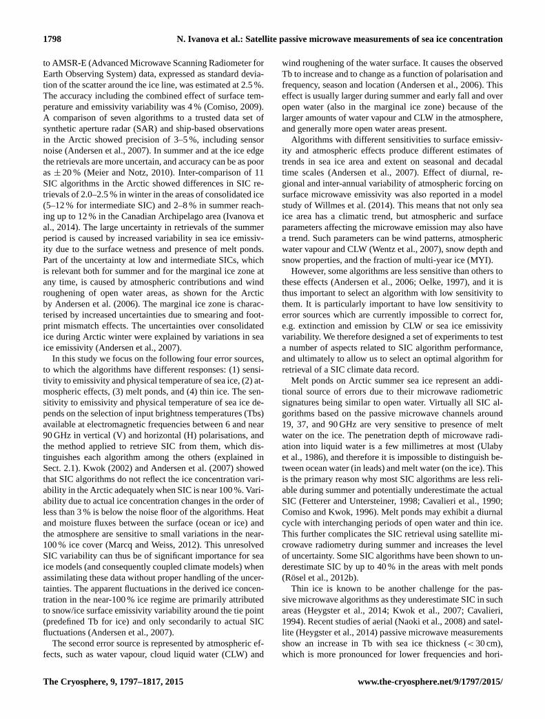
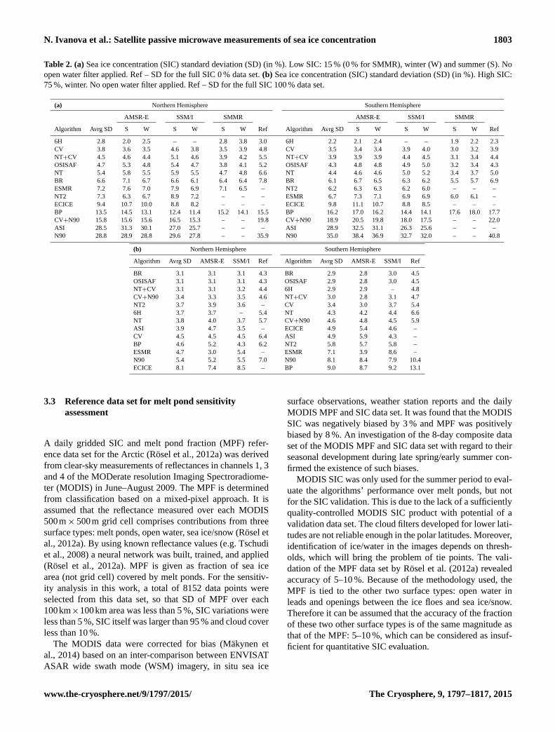
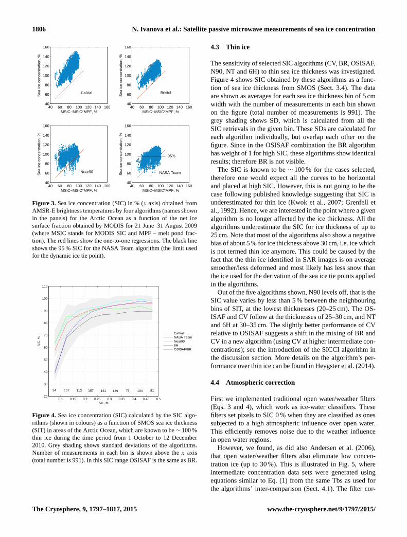
Figure 3 shows SIC calculated by four selected SIC algo-
rithms (CV, BR, N90 and NT) as a function of C. Note that
because of the limitation to MSIC > 95 % the variation in the
net ice surface fraction is almost solely due to the variation
in MPF, which was varying from 0 to 50 % for the selected
data set.
There is a pronounced overestimation of the net ice surface
fraction by the CV and BR algorithms that compose the OS-
ISAF combination (however only BR is used for high SIC).
For example, at C = 90 % the average SIC is 128 % (CV),
115 % (BR), 103 % (N90) and 100 % (NT). The slopes of the
regression lines are close to one (0.9–1.2 for the shown al-
gorithms), which agrees with the assumption that melt ponds
are interpreted as open water by microwave radiometry. The
NT algorithm shows SIC values closest to C (the least bias
of the four algorithms), which adds to our argument for using
this algorithm for defining areas of high SIC (NT > 95 %) for
retrieval of the dynamic tie points (Sect. 4.5).
www.the-cryosphere.net/9/1797/2015/ The Cryosphere, 9, 1797–1817, 2015
1806 N. Ivanova et al.: Satellite passive microwave measurements of sea ice concentration
40 60 80 100 120 140 16040
60
80
100
120
140
160
MSIC−MSIC*MPF, %
Sea
ice
conc
entr
atio
n, %
40 60 80 100 120 140 16040
60
80
100
120
140
160
MSIC−MSIC*MPF, %
Sea
ice
conc
entr
atio
n, %
40 60 80 100 120 140 16040
60
80
100
120
140
160
MSIC−MSIC*MPF, %
Sea
ice
conc
entr
atio
n, %
40 60 80 100 120 140 16040
60
80
100
120
140
160
MSIC−MSIC*MPF, %
Sea
ice
conc
entr
atio
n, %
CalVal Bristol
Near90
95%
NASA Team
Figure 3. Sea ice concentration (SIC) in % (y axis) obtained from
AMSR-E brightness temperatures by four algorithms (names shown
in the panels) for the Arctic Ocean as a function of the net ice
surface fraction obtained by MODIS for 21 June–31 August 2009
(where MSIC stands for MODIS SIC and MPF – melt pond frac-
tion). The red lines show the one-to-one regressions. The black line
shows the 95 % SIC for the NASA Team algorithm (the limit used
for the dynamic ice tie point).
0.1 0.15 0.2 0.25 0.3 0.35 0.4 0.45 0.520
30
40
50
60
70
80
90
100
110
SIT, m
SIC
, %
CalValNASA TeamNear906HOSISAF/BR
34 107 113 141187 149 75 104 81
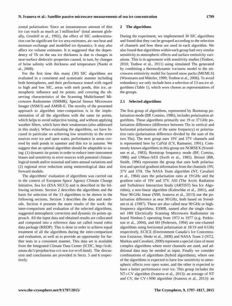
Figure 4. Sea ice concentration (SIC) calculated by the SIC algo-
rithms (shown in colours) as a function of SMOS sea ice thickness
(SIT) in areas of the Arctic Ocean, which are known to be ∼ 100 %
thin ice during the time period from 1 October to 12 December
2010. Grey shading shows standard deviations of the algorithms.
Number of measurements in each bin is shown above the x axis
(total number is 991). In this SIC range OSISAF is the same as BR.
4.3 Thin ice
The sensitivity of selected SIC algorithms (CV, BR, OSISAF,
N90, NT and 6H) to thin sea ice thickness was investigated.
Figure 4 shows SIC obtained by these algorithms as a func-
tion of sea ice thickness from SMOS (Sect. 3.4). The data
are shown as averages for each sea ice thickness bin of 5 cm
width with the number of measurements in each bin shown
on the figure (total number of measurements is 991). The
grey shading shows SD, which is calculated from all the
SIC retrievals in the given bin. These SDs are calculated for
each algorithm individually, but overlap each other on the
figure. Since in the OSISAF combination the BR algorithm
has weight of 1 for high SIC, these algorithms show identical
results; therefore BR is not visible.
The SIC is known to be ∼ 100 % for the cases selected,
therefore one would expect all the curves to be horizontal
and placed at high SIC. However, this is not going to be the
case following published knowledge suggesting that SIC is
underestimated for thin ice (Kwok et al., 2007; Grenfell et
al., 1992). Hence, we are interested in the point where a given
algorithm is no longer affected by the ice thickness. All the
algorithms underestimate the SIC for ice thickness of up to
25 cm. Note that most of the algorithms also show a negative
bias of about 5 % for ice thickness above 30 cm, i.e. ice which
is not termed thin ice anymore. This could be caused by the
fact that the thin ice identified in SAR images is on average
smoother/less deformed and most likely has less snow than
the ice used for the derivation of the sea ice tie points applied
in the algorithms.
Out of the five algorithms shown, N90 levels off, that is the
SIC value varies by less than 5 % between the neighbouring
bins of SIT, at the lowest thicknesses (20–25 cm). The OS-
ISAF and CV follow at the thicknesses of 25–30 cm, and NT
and 6H at 30–35 cm. The slightly better performance of CV
relative to OSISAF suggests a shift in the mixing of BR and
CV in a new algorithm (using CV at higher intermediate con-
centrations); see the introduction of the SICCI algorithm in
the discussion section. More details on the algorithm’s per-
formance over thin ice can be found in Heygster et al. (2014).
4.4 Atmospheric correction
First we implemented traditional open water/weather filters
(Eqs. 3 and 4), which work as ice-water classifiers. These
filters set pixels to SIC 0 % when they are classified as ones
subjected to a high atmospheric influence over open water.
This efficiently removes noise due to the weather influence
in open water regions.
However, we found, as did also Andersen et al. (2006),
that open water/weather filters also eliminate low concen-
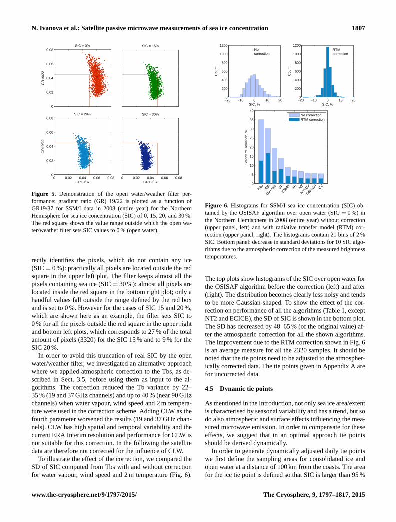
tration ice (up to 30 %). This is illustrated in Fig. 5, where
intermediate concentration data sets were generated using
equations similar to Eq. (1) from the same Tbs as used for
the algorithms’ inter-comparison (Sect. 4.1). The filter cor-
The Cryosphere, 9, 1797–1817, 2015 www.the-cryosphere.net/9/1797/2015/
N. Ivanova et al.: Satellite passive microwave measurements of sea ice concentration 1807
0
0.02
0.04
0.06
0.08
GR
19/2
2SIC = 0% SIC = 15%
0 0.02 0.04 0.06 0.080
0.02
0.04
0.06
0.08
GR
19/2
2
GR19/37
SIC = 20%
0 0.02 0.04 0.06 0.08GR19/37
SIC = 30%
Figure 5. Demonstration of the open water/weather filter per-
formance: gradient ratio (GR) 19/22 is plotted as a function of
GR19/37 for SSM/I data in 2008 (entire year) for the Northern
Hemisphere for sea ice concentration (SIC) of 0, 15, 20, and 30 %.
The red square shows the value range outside which the open wa-
ter/weather filter sets SIC values to 0 % (open water).
rectly identifies the pixels, which do not contain any ice
(SIC= 0 %): practically all pixels are located outside the red
square in the upper left plot. The filter keeps almost all the
pixels containing sea ice (SIC = 30 %): almost all pixels are
located inside the red square in the bottom right plot; only a
handful values fall outside the range defined by the red box
and is set to 0 %. However for the cases of SIC 15 and 20 %,
which are shown here as an example, the filter sets SIC to
0 % for all the pixels outside the red square in the upper right
and bottom left plots, which corresponds to 27 % of the total
amount of pixels (3320) for the SIC 15 % and to 9 % for the
SIC 20 %.
In order to avoid this truncation of real SIC by the open
water/weather filter, we investigated an alternative approach
where we applied atmospheric correction to the Tbs, as de-
scribed in Sect. 3.5, before using them as input to the al-
gorithms. The correction reduced the Tb variance by 22–
35 % (19 and 37 GHz channels) and up to 40 % (near 90 GHz
channels) when water vapour, wind speed and 2 m tempera-
ture were used in the correction scheme. Adding CLW as the
fourth parameter worsened the results (19 and 37 GHz chan-
nels). CLW has high spatial and temporal variability and the
current ERA Interim resolution and performance for CLW is
not suitable for this correction. In the following the satellite
data are therefore not corrected for the influence of CLW.
To illustrate the effect of the correction, we compared the
SD of SIC computed from Tbs with and without correction
for water vapour, wind speed and 2 m temperature (Fig. 6).
−20 −10 0 10 200
200
400
600
800
1000
1200
SIC, %
Cou
nt
−20 −10 0 10 200
200
400
600
800
1000
1200
SIC, %
Cou
nt
0
5
10
15
20
25
30
35
40
Sta
ndar
d D
evia
tion,
%
N90 ASI
CV+N90 BP
ESMR BR NT
NT+CV
OSISAF CV
No correctionRTM correction
Nocorrection
RTMcorrection
Figure 6. Histograms for SSM/I sea ice concentration (SIC) ob-
tained by the OSISAF algorithm over open water (SIC = 0 %) in
the Northern Hemisphere in 2008 (entire year) without correction
(upper panel, left) and with radiative transfer model (RTM) cor-
rection (upper panel, right). The histograms contain 21 bins of 2 %
SIC. Bottom panel: decrease in standard deviations for 10 SIC algo-
rithms due to the atmospheric correction of the measured brightness
temperatures.
The top plots show histograms of the SIC over open water for
the OSISAF algorithm before the correction (left) and after
(right). The distribution becomes clearly less noisy and tends
to be more Gaussian-shaped. To show the effect of the cor-
rection on performance of all the algorithms (Table 1, except
NT2 and ECICE), the SD of SIC is shown in the bottom plot.
The SD has decreased by 48–65 % (of the original value) af-
ter the atmospheric correction for all the shown algorithms.
The improvement due to the RTM correction shown in Fig. 6
is an average measure for all the 2320 samples. It should be
noted that the tie points need to be adjusted to the atmospher-
ically corrected data. The tie points given in Appendix A are
for uncorrected data.
4.5 Dynamic tie points
As mentioned in the Introduction, not only sea ice area/extent
is characterised by seasonal variability and has a trend, but so
do also atmospheric and surface effects influencing the mea-
sured microwave emission. In order to compensate for these
effects, we suggest that in an optimal approach tie points
should be derived dynamically.
In order to generate dynamically adjusted daily tie points
we first define the sampling areas for consolidated ice and
open water at a distance of 100 km from the coasts. The area
for the ice tie point is defined so that SIC is larger than 95 %
www.the-cryosphere.net/9/1797/2015/ The Cryosphere, 9, 1797–1817, 2015
1808 N. Ivanova et al.: Satellite passive microwave measurements of sea ice concentration
according to the NT algorithm and it is within the limits of
maximum sea ice extent climatology (NSIDC, 1979–2007).
The NT algorithm was chosen for this purpose because it
is a standard relatively simple algorithm with little sensitiv-
ity to ice temperature variations (Cavalieri et al., 1984). The
data for the open water tie point were selected geographically
along two belts in the Northern and Southern hemispheres
defined by the maximum sea ice extent climatology (200 km
wide belt starting 150 km away from the climatology). Data
points south of 50N were not used. A total of 15 000 data
points per day were selected.
Then 5000 Tb measurements (every day) in these areas
were randomly selected among the total of 15 000 data points
and averaged using a 15-day running window (± 7 days)
to reduce potential noise in daily values. Selection of only
5000 samples per day is to ensure that no days are weighted
higher than others when there are differences in the number
of data points from day to day. The 15-day window allows
smoothing out of the synoptic scales of weather perturba-
tions and at the same time capture the onset of ice emissivity
changes due to summer melt or fall freeze-up. We believe
that longer time windows will induce too much smoothing
over the ice, while shorter time-periods will introduce too
much noise (over open water). The scatter of all the obtained
15 000 data points per day was used as a tie point uncertainty,
which contributes to the total per-pixel daily uncertainty re-
trieved for SIC.
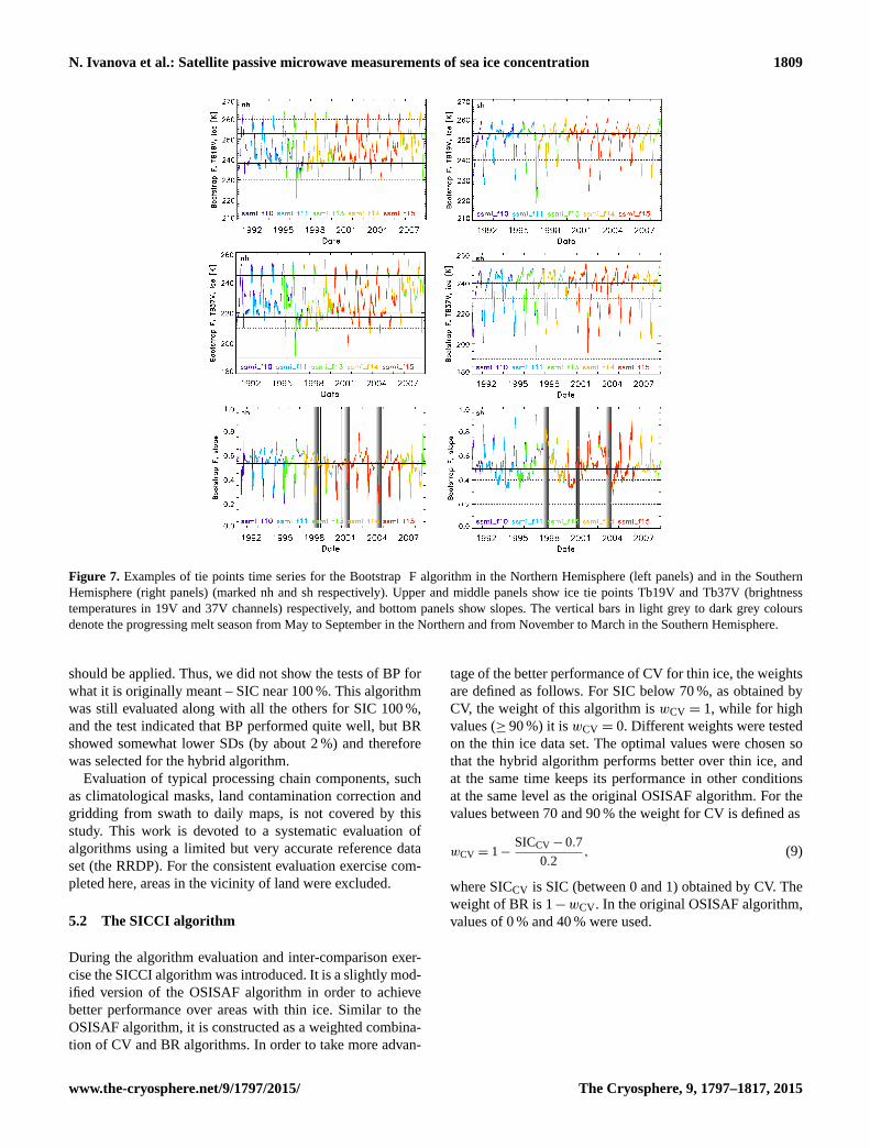
An example of an ice tie point is shown in Fig. 7 by Tb19V
and Tb37V (top and middle panels) and slope of the ice
line according to the Bootstrap scheme (bottom panels). We
chose to not show the tie points of the Bristol algorithm be-
cause the polarisation and frequency information from 19V,
37V and 37H channels is transformed into a 2-D plane de-
fined by x and y components (see Smith, 1996 for more de-
tails), which are harder to relate to than Tbs. The open wa-
ter tie points are not shown here as they have less seasonal
variability (within 5 K). The dynamic tie point for ice is rep-
resented by an average of the fraction of FYI and MYI in
the samples of all (± 7 days) selected ice conditions (NT
> 95 %). Due to the change in the relative amount of FYI
and MYI in the Arctic Ocean in recent years, the average ice
tie point will move along the ice line in the Tb space.
Figure 7 demonstrates that the tie points are not constant
values as it is assumed traditionally (static tie points from
the RRDP, also averaged FYI and MYI values, are shown by
horizontal lines), but rather geophysical parameters showing
seasonal and inter-annual variations. This applies particularly
to the melt season, which is highlighted by the grey vertical
bars for three selected years in Fig. 7, bottom plots. There-
fore the dynamic approach is more suitable for the SIC al-
gorithms. The ice tie point may vary by about 30 K during 1
year, which amounts to approximately 8–10 % of the average
value. Sensor drift and inter-sensor differences are also im-
portant aspects, which might cause an unrealistic trend in the
retrieved SIC when static tie points are applied. The dynamic
tie point approach compensates for these effects.
A detailed description of the procedure to obtain dynamic
tie points is given in the Appendix B. The tie points will vary
with calibration of the input data/version number and source,
so the tie points obtained here should not be used with other
versions of the input data with potentially different calibra-
tion. The procedure on the other hand can be applied to all
versions/calibrations of the input data.
5 Discussion
5.1 Algorithms inter-comparison and selection
Based on validation data sets of SIC 15 and 75 % we used
variability (SD) in the SIC produced by the different algo-
rithms as a measure of the sensitivity to geophysical error
sources and instrumental noise. The errors from geophysi-
cal sources over open water are generated by wind induced
surface roughness, surface and atmospheric temperature vari-
ability and atmospheric water vapour and CLW. Over ice, the
errors are dominated by snow and ice emissivity and temper-
ature variability, where parameters such as snow depth, and
to some extent variability in snow density and ice emissivity
are important (Tonboe and Andersen, 2004). The atmosphere
plays only a minor role over ice except at near 90 GHz, where
liquid water/ice clouds may still be a significant error source,
especially in the marginal ice zone. At the same time near
90 GHz data might be less sensitive to changes in physical
properties in ice and snow because of the smaller penetration
depth relative to the other frequencies used.
The algorithms 6H, CV, BR, OSISAF, NT and NT+CV,
showed the lowest SDs (Table 2). The 6 GHz channel was
not available on SSM/I, which provides the longest time se-
ries, and therefore the 6H algorithm was not considered to
be an optimal SIC algorithm for a climate data set. Bristol
showed the lowest SD over high SIC (only winter is consid-
ered) while CV had the lowest SD for the low SIC cases,
which suggests that combining these two algorithms would
provide a good basis for an optimal SIC algorithm.
The differences in SDs between summer and winter are
reflecting the sensitivity of different algorithms to wind, at-
mospheric humidity and other seasonally changing quanti-
ties. In addition, some of these quantities may have climato-
logical trends. Therefore, small difference between the sum-
mer and winter SDs is an asset for an algorithm. The algo-
rithms NT, NT+CV, BR, CV and OSISAF showed the lowest
summer–winter differences in SD (0.2–0.3 % on average for
both hemispheres and all three instruments).
Note that the two modes of the Bootstrap algorithm in this
study were tested separately. The frequency mode (BF) of the
original algorithm is applied only when Tb19V is below the
ice line minus 5 K (Comiso, 1995), which is the case for both
the 15 and 75 % cases. Otherwise the polarisation mode (BP)
The Cryosphere, 9, 1797–1817, 2015 www.the-cryosphere.net/9/1797/2015/
N. Ivanova et al.: Satellite passive microwave measurements of sea ice concentration 1809
Figure 7. Examples of tie points time series for the Bootstrap F algorithm in the Northern Hemisphere (left panels) and in the Southern
Hemisphere (right panels) (marked nh and sh respectively). Upper and middle panels show ice tie points Tb19V and Tb37V (brightness
temperatures in 19V and 37V channels) respectively, and bottom panels show slopes. The vertical bars in light grey to dark grey colours
denote the progressing melt season from May to September in the Northern and from November to March in the Southern Hemisphere.
should be applied. Thus, we did not show the tests of BP for
what it is originally meant – SIC near 100 %. This algorithm
was still evaluated along with all the others for SIC 100 %,
and the test indicated that BP performed quite well, but BR
showed somewhat lower SDs (by about 2 %) and therefore
was selected for the hybrid algorithm.
Evaluation of typical processing chain components, such
as climatological masks, land contamination correction and
gridding from swath to daily maps, is not covered by this
study. This work is devoted to a systematic evaluation of
algorithms using a limited but very accurate reference data
set (the RRDP). For the consistent evaluation exercise com-
pleted here, areas in the vicinity of land were excluded.
5.2 The SICCI algorithm
During the algorithm evaluation and inter-comparison exer-
cise the SICCI algorithm was introduced. It is a slightly mod-
ified version of the OSISAF algorithm in order to achieve
better performance over areas with thin ice. Similar to the
OSISAF algorithm, it is constructed as a weighted combina-
tion of CV and BR algorithms. In order to take more advan-
tage of the better performance of CV for thin ice, the weights
are defined as follows. For SIC below 70 %, as obtained by
CV, the weight of this algorithm is wCV = 1, while for high
values (≥ 90 %) it is wCV = 0. Different weights were tested
on the thin ice data set. The optimal values were chosen so
that the hybrid algorithm performs better over thin ice, and
at the same time keeps its performance in other conditions
at the same level as the original OSISAF algorithm. For the
values between 70 and 90 % the weight for CV is defined as
wCV = 1−SICCV− 0.7
0.2, (9)
where SICCV is SIC (between 0 and 1) obtained by CV. The
weight of BR is 1−wCV. In the original OSISAF algorithm,
values of 0 % and 40 % were used.
www.the-cryosphere.net/9/1797/2015/ The Cryosphere, 9, 1797–1817, 2015
1810 N. Ivanova et al.: Satellite passive microwave measurements of sea ice concentration
5.3 Melt ponds
Figure 3 illustrates that the four algorithms shown (but this is
also valid for all other algorithms) are sensitive to the MPF,
which may mean that melt ponds are interpreted as open wa-
ter by the algorithms. This is because microwave penetration
into water is very small. Rösel et al. (2012b) showed that in
areas with melt ponds SIC algorithms (ASI, NT2 and Boot-
strap) underestimate SIC by up to 40 % (corresponding to
a MPF close to 40 %). One may still argue that melt ponds
should have different signature from that of open water due
to the difference in their salinity. However, for frequencies as
high as those used in the algorithms (19 GHz and higher) and
in cold water the salinity was found to play a less significant
role (Meissner and Wentz, 2012; see also Ulaby et al., 1986).
In addition, the footprint size is so large (e.g. 70km× 45km
for 19.3 GHz channel on SSM/I) that an unresolvable mix-
ture of surfaces might be present in it.
For some applications it is important to interpret ponded
ice as ice and not as open water. However, we believe that
satellite microwave radiometry is incapable of estimating
SIC correctly if a certain fraction of the sea ice is sub-
merged under water. Therefore, we suggest accepting what
microwave sensors actually can do: estimate the net ice sur-
face fraction. The latter is similar to the well known SIC dur-
ing most of the year until melt ponds have formed on top of
the ice in the melting season. Additional data sources (for
example MODIS) could be used to supplement summer re-
trievals of SIC. Unlike with microwave radiometry, open wa-
ter in leads and openings between the ice floes can be dis-
criminated from open water in melt ponds on ice floes by
means of their different optical spectral properties.
The algorithms shown in Fig. 3 overestimate SIC, which
can be caused by higher Tbs in the areas between melt ponds.
During summer these areas comprise wet snow and/or bare
ice with a different physical structure than during winter.
Therefore these areas have radiometric properties potentially
different from those of winter, when the RRDP ice tie points
were developed. This is demonstrated by Fig. 7 where the
grey bars highlight that seasonal changes in the dynamic tie
points to be used in the SICCI algorithm vary particularly
during the summer months. The comparison of passive mi-
crowave algorithms and MODIS SIC in Rösel et al. (2012b)
showed that in the areas without melt ponds the passive mi-
crowave SIC was larger than that of MODIS. Note also, how-
ever, that the tie points used here differ from those in Rösel
et al. (2012b). This complicates a quantitative comparison of
their results with ours and, in turn, calls for such kind of sys-
tematic, consistent evaluation and inter-comparison as shown
in the present paper. Using the dynamic tie points approach
(Sect. 4.5) decreases this effect: the OSISAF algorithm on
average overestimated SIC by 24 % when fixed RRDP tie
points were used (same as in the Fig. 3) and by 17 % with
dynamical tie points (this example is not shown in the fig-
ure). However, even with dynamic tie points, it is likely that
the areas selected to derive the 100 % ice tie point during
summer contain melt ponds. If this would be the case and if
the selected area would have an average melt pond fraction of
10 %, then the 100 % ice tie point would not represent 100 %
ice but a net ice surface fraction of only 90 %. When estimat-
ing dynamic tie points, an initial SIC estimate is needed. In
our case this was done using pixels with NT SIC > 95 %.
This algorithm is less sensitive to the surface temperature
variations because it is based on polarisation and gradient
ratios of Tbs, which more or less cancels out the physical
temperature (Cavalieri et al., 1984). In addition, it is inter-
preting melt ponds as open water (Sect. 4.2). This means that
using NT SIC > 95 % we select areas with reasonably low
MPF to determine the signature of ice, which helps to avoid
contamination of ice tie point by measurements containing
melt ponds. A much more detailed discussion of the results
for melt ponds is underway in a separate paper.
Another relevant aspect is effect of refrozen melt ponds on
passive microwave signatures, which was not addressed in
this study. It has not yet been covered thoroughly in the liter-
ature (except Comiso and Kwok, 1996) and thus represents
an interesting topic for future studies. Per definition, refrozen
melt ponds occur on the MYI and they are formed of fresh
water, which means these two surfaces have different density
and structure with presumably much less air bubbles in the
refrozen melt pond than in MYI. This may partially explain
the large variability in MYI signatures.
5.4 Thin ice
All the algorithms shown for the thin ice test (Fig. 4) under-
estimate the SIC for ice thicknesses up to 35 cm, which con-
firms findings by others (see Introduction). The 6H algorithm
showed the highest sensitivity to the sea ice thickness, which
is in agreement with Scott et al. (2014) showing that Tbs at
6 GHz can be used to estimate thin ice thickness. The least
sensitivity to thickness of thin ice was observed for the N90
algorithm; the SIC obtained by this algorithm was indepen-
dent of SIT values already at thicknesses of 20–25 cm. This
is caused most likely by a smaller penetration depth in the
near-90 GHz channels (shorter wave length) (see also Gren-
fell et al., 1998). OSISAF and CV had the second least sen-
sitivity (levelled off at 25–30 cm), which adds more weight
to the choice of an OSISAF-like combination as an optimal
algorithm. We suggest that, when areas of thin ice are inter-
preted as reduced concentration, this should be clearly stated
along with an eventual SIC product. This issue is similar to
melt ponds in a way that there is no simple solution, and one
should be aware of the limitation, which we demonstrate by
the Fig. 4. In this study we manage to quantify the effect and
thus allow modellers to assimilate SIC data in a more proper
way. Implementation of an algorithm that accounts for thin
ice (Röhrs and Kaleschke, 2012; Röhrs et al., 2012; Naoki
et al., 2008; Grenfell et al., 1992) as an additional module to
this optimal algorithm could be a potential improvement. For
The Cryosphere, 9, 1797–1817, 2015 www.the-cryosphere.net/9/1797/2015/
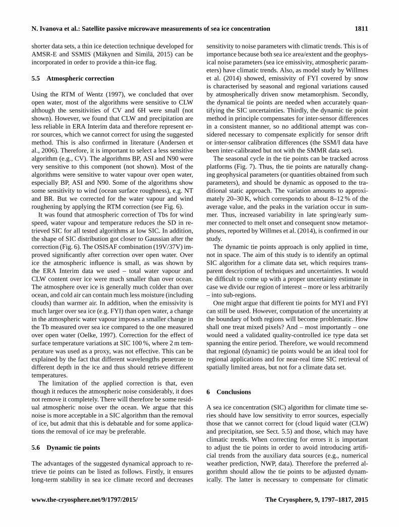
N. Ivanova et al.: Satellite passive microwave measurements of sea ice concentration 1811
shorter data sets, a thin ice detection technique developed for
AMSR-E and SSMIS (Mäkynen and Similä, 2015) can be
incorporated in order to provide a thin-ice flag.
5.5 Atmospheric correction
Using the RTM of Wentz (1997), we concluded that over
open water, most of the algorithms were sensitive to CLW
although the sensitivities of CV and 6H were small (not
shown). However, we found that CLW and precipitation are
less reliable in ERA Interim data and therefore represent er-
ror sources, which we cannot correct for using the suggested
method. This is also confirmed in literature (Andersen et
al., 2006). Therefore, it is important to select a less sensitive
algorithm (e.g., CV). The algorithms BP, ASI and N90 were
very sensitive to this component (not shown). Most of the
algorithms were sensitive to water vapour over open water,
especially BP, ASI and N90. Some of the algorithms show
some sensitivity to wind (ocean surface roughness), e.g. NT
and BR. But we corrected for the water vapour and wind
roughening by applying the RTM correction (see Fig. 6).
It was found that atmospheric correction of Tbs for wind
speed, water vapour and temperature reduces the SD in re-
trieved SIC for all tested algorithms at low SIC. In addition,
the shape of SIC distribution got closer to Gaussian after the
correction (Fig. 6). The OSISAF combination (19V/37V) im-
proved significantly after correction over open water. Over
ice the atmospheric influence is small, as was shown by
the ERA Interim data we used – total water vapour and
CLW content over ice were much smaller than over ocean.
The atmosphere over ice is generally much colder than over
ocean, and cold air can contain much less moisture (including
clouds) than warmer air. In addition, when the emissivity is
much larger over sea ice (e.g. FYI) than open water, a change
in the atmospheric water vapour imposes a smaller change in
the Tb measured over sea ice compared to the one measured
over open water (Oelke, 1997). Correction for the effect of
surface temperature variations at SIC 100 %, where 2 m tem-
perature was used as a proxy, was not effective. This can be
explained by the fact that different wavelengths penetrate to
different depth in the ice and thus should retrieve different
temperatures.
The limitation of the applied correction is that, even
though it reduces the atmospheric noise considerably, it does
not remove it completely. There will therefore be some resid-
ual atmospheric noise over the ocean. We argue that this
noise is more acceptable in a SIC algorithm than the removal
of ice, but admit that this is debatable and for some applica-
tions the removal of ice may be preferable.
5.6 Dynamic tie points
The advantages of the suggested dynamical approach to re-
trieve tie points can be listed as follows. Firstly, it ensures
long-term stability in sea ice climate record and decreases
sensitivity to noise parameters with climatic trends. This is of
importance because both sea ice area/extent and the geophys-
ical noise parameters (sea ice emissivity, atmospheric param-
eters) have climatic trends. Also, as model study by Willmes
et al. (2014) showed, emissivity of FYI covered by snow
is characterised by seasonal and regional variations caused
by atmospherically driven snow metamorphism. Secondly,
the dynamical tie points are needed when accurately quan-
tifying the SIC uncertainties. Thirdly, the dynamic tie point
method in principle compensates for inter-sensor differences
in a consistent manner, so no additional attempt was con-
sidered necessary to compensate explicitly for sensor drift
or inter-sensor calibration differences (the SSM/I data have
been inter-calibrated but not with the SMMR data set).
The seasonal cycle in the tie points can be tracked across
platforms (Fig. 7). Thus, the tie points are naturally chang-
ing geophysical parameters (or quantities obtained from such
parameters), and should be dynamic as opposed to the tra-
ditional static approach. The variation amounts to approxi-
mately 20–30 K, which corresponds to about 8–12 % of the
average value, and the peaks in the variation occur in sum-
mer. Thus, increased variability in late spring/early sum-
mer connected to melt onset and consequent snow metamor-
phoses, reported by Willmes et al. (2014), is confirmed in our
study.
The dynamic tie points approach is only applied in time,
not in space. The aim of this study is to identify an optimal
SIC algorithm for a climate data set, which requires trans-
parent description of techniques and uncertainties. It would
be difficult to come up with a proper uncertainty estimate in
case we divide our region of interest – more or less arbitrarily
– into sub-regions.
One might argue that different tie points for MYI and FYI
can still be used. However, computation of the uncertainty at
the boundary of both regions will become problematic. How
shall one treat mixed pixels? And – most importantly – one
would need a validated quality-controlled ice type data set
spanning the entire period. Therefore, we would recommend
that regional (dynamic) tie points would be an ideal tool for
regional applications and for near-real time SIC retrieval of
spatially limited areas, but not for a climate data set.
6 Conclusions
A sea ice concentration (SIC) algorithm for climate time se-
ries should have low sensitivity to error sources, especially
those that we cannot correct for (cloud liquid water (CLW)
and precipitation, see Sect. 5.5) and those, which may have
climatic trends. When correcting for errors it is important
to adjust the tie points in order to avoid introducing artifi-
cial trends from the auxiliary data sources (e.g., numerical
weather prediction, NWP, data). Therefore the preferred al-
gorithm should allow the tie points to be adjusted dynam-
ically. The latter is necessary to compensate for climatic
www.the-cryosphere.net/9/1797/2015/ The Cryosphere, 9, 1797–1817, 2015
1812 N. Ivanova et al.: Satellite passive microwave measurements of sea ice concentration
changes in the radiometric signature of ice and water, as well
as eventual instrumental drift and inter-instrument bias. In
addition, this algorithm should be accurate over the whole
range of SIC from 0 to 100 %. Along the ice edge spatial
resolution and sensitivity to new ice and atmospheric ef-
fects is of particular concern. In order to produce a long
climate data record, it is also important that the algorithm
is based on a selection of channels for which the process-
ing of long time-series is possible, which are currently 19
and 37 GHz. The comprehensive algorithm inter-comparison
study reported here leads to following conclusions.
– The CalVal algorithm is among the best (low standard
deviation (SD), Table 2a) of the simple algorithms at
low SIC and over open water.
– The Bristol algorithm is the best (lowest SD, Table 2b)
for high SIC.
– OSISAF-like combination of CalVal and Bristol is a
good choice for an overall algorithm, using CalVal at
low SIC and Bristol at high SIC.
In addition we conclude that
– Melt ponds are interpreted as open water by all algo-
rithms.
– Thin ice is seen as reduced SIC by all algorithms.
– After atmospheric correction of Tbs, low SIC became
less uncertain (less noisy) than high SIC.
– Near 90 GHz algorithms are very sensitive to atmo-
spheric effects at low SIC.
– All 10 algorithms shown in the Fig. 6 improve substan-
tially when brightness temperatures (Tbs) are corrected
for atmospheric effects using radiative transfer model
(RTM) with NWP data. The additional 3 algorithms by
nature could not be corrected/tested for this.
– The dynamic tie points approach can reduce systematic
biases in SIC and alleviate the seasonal variability in
SIC accuracy.
It is clear from these conclusions that there is no one sin-
gle algorithm that is superior in all criteria, and it seems that
a combination of algorithms (e.g., OSISAF or SICCI) is a
good choice. An additional advantage of using a set of 19
and 37 GHz algorithms is that the data set extends from fall
1978 until today and into the foreseeable future.
Over ice the Bristol algorithm, chosen for the high SIC
retrievals, is sensitive to the snow and ice temperature profile
as well as to ice emissivity variations. Surface temperature is
quantified in most NWP models, which means that there is a
potential for correction. The Bristol algorithm performance
over melting ice is good because the SIC as a function of
net ice surface fraction has a slope close to one. The Bristol
algorithm as other algorithms has a clear seasonal cycle in the
apparent ice concentration at 100 % SIC when using static tie
points. This means that dynamic tie points are an advantage
when using Bristol (as with most of the other algorithms).
Over open water the CalVal algorithm, chosen for the low
SIC retrievals, is among the algorithms with the lowest over-
all sensitivity to error sources including surface temperature,
wind, and atmospheric water vapour. Importantly, the CalVal
is relatively insensitive to CLW, which is a parameter we can-
not correct for due to the uncertainty of this parameter in the
NWP data at high latitudes. The response of CalVal to atmo-
spheric correction gives a substantial reduction in the noise
level. The response of CalVal to thin ice is better than that of
the other 19 and 37 GHz algorithms and comparable to near
90 GHz algorithms.
Therefore we suggest that an OSISAF or SICCI type of al-
gorithm with dynamic tie points and atmospheric correction
could be a good choice for SIC climate data set retrievals.
The selection of tie points should be done with careful atten-
tion to the melt pond issues in order to avoid melt pond con-
tamination of the tie points in summer. Correction for wind
speed, water vapour and surface temperature provides a clear
noise reduction, but we found no improvement from correct-
ing for NWP CLW.
In spite of their high resolution and good skill over ice, the
near-90 GHz algorithms have some limitations for a SIC cli-
mate data set because the near-90 GHz data were not avail-
able before 1991, and they are very sensitive to the atmo-
spheric error sources over open water and near ice edge
such as CLW. Finer spatial resolution achieved by the high-
frequency channels does not reduce the weather-induced SIC
errors over open water and near ice edge. Model data used in
the RTM to correct for the influence of surface wind speed,
water vapour and air temperature have a coarser spatial reso-
lution, and hence will cause artifacts in the RTM-based cor-
rection. The remaining weather effects we cannot correct for
(CLW and precipitation) will become even worse and more
difficult to correct for because the model is even less capa-
ble of providing the information for this parameters at the
same spatial scale as would be required. Their skill over ice
is approximately the same as the one of the selected Bristol
algorithm.
In the presented work we suggested a number of param-
eters, which could be used in order to select an optimal ap-
proach to retrieval of SIC climate data set. We also suggested
an approach that satisfies these requirements. However, we
do not claim the suggested approach to be the best one, tak-
ing into account that there is still a lot of potential for im-
provement in passive microwave methods.
The Cryosphere, 9, 1797–1817, 2015 www.the-cryosphere.net/9/1797/2015/
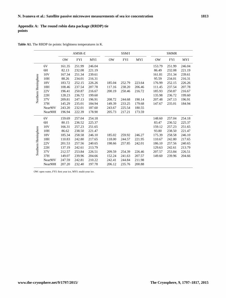
N. Ivanova et al.: Satellite passive microwave measurements of sea ice concentration 1813
Appendix A: The round robin data package (RRDP) tie
points
Table A1. The RRDP tie points: brightness temperatures in K.
AMSR-E SSM/I SMMR
OW FYI MYI OW FYI MYI OW FYI MYI
No
rth
ern
Hem
isp
her
e
6V 161.35 251.99 246.04 153.79 251.99 246.04
6H 82.13 232.08 221.19 86.49 232.08 221.19
10V 167.34 251.34 239.61 161.81 251.34 239.61
10H 88.26 234.01 216.31 95.59 234.01 216.31
18V 183.72 252.15 226.26 185.04 252.79 223.64 176.99 252.15 226.26
18H 108.46 237.54 207.78 117.16 238.20 206.46 111.45 237.54 207.78
22V 196.41 250.87 216.67 200.19 250.46 216.72 185.93 250.87 216.67
22H 128.23 236.72 199.60 135.98 236.72 199.60
37V 209.81 247.13 196.91 208.72 244.68 190.14 207.48 247.13 196.91
37H 145.29 235.01 184.94 149.39 233.25 179.68 147.67 235.01 184.94
Near90V 243.20 232.01 187.60 243.67 225.54 180.55
Near90H 196.94 222.39 178.90 205.73 217.21 173.59
So
uth
ern
Hem
isp
her
e
6V 159.69 257.04 254.18 148.60 257.04 254.18
6H 80.15 236.52 225.37 83.47 236.52 225.37
10V 166.31 257.23 251.65 159.12 257.23 251.65
10H 86.62 238.50 221.47 93.80 238.50 221.47
18V 185.34 258.58 246.10 185.02 259.92 246.27 175.39 258.58 246.10
18H 110.83 242.80 217.65 118.00 244.57 221.95 110.67 242.80 217.65
22V 201.53 257.56 240.65 198.66 257.85 242.01 186.10 257.56 240.65
22H 137.19 242.61 213.79 129.63 242.61 213.79
37V 212.57 253.84 226.51 209.59 254.39 226.46 207.57 253.84 226.51
37H 149.07 239.96 204.66 152.24 241.63 207.57 149.60 239.96 204.66
Near90V 247.59 242.81 210.22 242.41 244.84 211.98
Near90H 207.20 232.40 197.78 206.12 235.76 200.88
OW: open water, FYI: first year ice, MYI: multi-year ice.
www.the-cryosphere.net/9/1797/2015/ The Cryosphere, 9, 1797–1817, 2015
1814 N. Ivanova et al.: Satellite passive microwave measurements of sea ice concentration
Appendix B: Retrieval of the dynamic tie points
Computing of the dynamic tie points involves two steps.
First, a large number of characteristic Tb samples are se-
lected for each day. Then, these data samples are aggregated
over a temporal sliding window.
B1 The open water tie point
The open water data samples are selected geographically
within the limits of two 200 km wide belts, one in each hemi-
sphere. Each belt follows the mask of a maximum sea ice ex-
tent climatology, which was first extended 150 km away from
the pole of the respective hemisphere. A land mask extending
100 km into open sea ensures that the open water signatures
are not contaminated by land spill-over effects. In the North-
ern Hemisphere, data points south of 50N are discarded. A
maximum of 5000 randomly selected open water data sam-
ples are kept per day.
The daily open water tie point is computed as the average
Tb of all selected open water data samples in a centred tem-
poral sliding window (± 7 days). The open water tie point is
computed separately for each hemisphere.
B2 The sea ice tie point
The sea ice data samples are selected geographically within
a maximum sea ice extent climatology for each hemisphere.
The ice tie point data must in addition correspond to a SIC
greater than 95 %, as retrieved by the NASA Team algorithm
using the tie points from the Appendix A. Additional masks
ensure that samples are taken away from the coastal regions.
A maximum of 5000 sea ice data samples are kept per day.
The daily sea ice tie point is computed over the same tem-
poral sliding window as the open water tie point, and is com-
puted separately for each hemisphere. The slope and offset
of the ice line are computed using principal component anal-
ysis. The ice line is the line in Tb space that goes through the
FYI and MYI points (type-A and type-B ice in the Southern
Hemisphere, see Figs. 1 and 2). Since the total SIC is our
target (and not the partial concentrations of ice types), alter-
native versions of the CV and Bristol algorithms that rely on
the slope and offset of the ice line were implemented. Ad-
ditional criteria would be needed for further splitting the sea
ice data samples into tie points based on ice types; this is not
considered here.
A similar approach to deriving dynamic tie points is im-
plemented for the sea ice concentration reprocessed data set,
and operational products of the EUMETSAT OSISAF.
The Cryosphere, 9, 1797–1817, 2015 www.the-cryosphere.net/9/1797/2015/
N. Ivanova et al.: Satellite passive microwave measurements of sea ice concentration 1815
Acknowledgements. This work was completed in the context
of ESA Climate Change Initiative, Sea Ice project (SICCI) and
was funded by ESA. The work of S. Kern was supported by the
Center of Excellence for Climate System Analysis and Prediction
(CliSAP). Support from the International Space Science Institute
(ISSI), Bern, Switzerland, under project No. 245: Perta Heil
and Stefan Kern, “Towards an integrated retrieval of Antarctic
sea ice volume” is acknowledged. The EUMETSAT OSISAF
(http://osisaf.met.no) granted access to an implementation of
its SIC processing software, in particular the dynamic tie point
retrieval process (see Appendix B). The authors would like to thank
Timothy Williams and Richard Danielson for their proofreading of
the manuscript.
Edited by: C. Haas
References
Andersen, S., Tonboe, R., Kern, S., and Schyberg, H.: Improved re-
trieval of sea ice total concentration from spaceborne passive mi-
crowave observations using numerical weather prediction model
fields: an intercomparison of nine algorithms, Remote Sens. En-
viron., 104, 374–392, 2006.
Andersen, S., Tonboe, R., Kaleschke, L., Heygster, G., and Peder-
sen, L. T.: Intercomparison of passive microwave sea ice concen-
tration retrievals over the high-concentration Arctic sea ice, J.
Geophys. Res., 112, C08004, doi:10.1029/2006JC003543, 2007.
Ashcroft, P. and Wentz, F. J.: AMSR-E/Aqua L2A Global Swath
Spatially-Resampled Brightness Temperatures, Version 2, NASA
DAAC at the National Snow and Ice Data Center, Boulder, Col-
orado USA, doi:10.5067/AMSR-E/AE_L2A.002, 2003.
Brucker, L., Cavalieri, D. J., Markus, T., and Ivanoff, A.:
NASA Team 2 Sea Ice Concentration Algorithm Retrieval
Uncertainty, IEEE T. Geosci. Remote, 52, 7336–7352,
doi:10.1109/TGRS.2014.2311376, 2014.
Cavalieri, D. J.: A microwave technique for mapping thin sea ice,
J. Geophys. Res., 99, 12561–12572, doi:10.1029/94JC00707,
1994.
Cavalieri, D. J. and Parkinson, C. L.: Arctic sea ice variability and
trends, 1979–2010, The Cryosphere, 6, 881–889, doi:10.5194/tc-
6-881-2012, 2012.
Cavalieri, D. J., Gloersen, P., and Campbell, W. J.: Determination
of sea ice parameters with the NIMBUS 7 SMMR, J. Geophys.
Res., 89, 5355–5369, 1984.
Cavalieri, D. J., Burns, B. A., and Onstott, R. G.: Investigation of the
effects of summer melt on the calculation of sea ice concentration
using active and passive microwave data, J. Geophys. Res., 95,
5359–5369, 1990.
Cavalieri, D. J., Germain, K. S., and Swift, C. T.: Reduction of
weather effects in the calculation of sea ice concentration with
the DMSP SSM/I, J. Glaciol., 41, 455–464, 1995.
Comiso, J. C.: Characteristics of arctic winter sea ice from satel-
lite multispectral microwave observations, J. Geophys. Res., 91,
975–994, 1986.
Comiso, J. C.: SSM/I Sea Ice Concentrations Using the Boot-
strap Algorithm, NASA Reference Publication 1380, NASA
Center for Aerospace Information, 800 Elkridge Landing Road,
Linthicum Heights, MD 21090-2934, (301) 621-0390, 1995.
Comiso, J. C.: Enhanced Sea Ice Concentrations and Ice Extents
from AMSR-E Data, Journal of The Remote Sensing Society of
Japan, 29, 199–215, doi:10.11440/rssj.29.199, 2009.
Comiso, J. C. and Kwok, R.: Surface and radiative characteristics
of the summer Arctic sea ice cover from multisensor satellite ob-
servations, J. Geophys. Res., 101, 28397–28416, 1996.
Eastwood, S. (Ed.): Ocean & Sea Ice SAF (OSISAF) Sea Ice Prod-
uct Manual, Version 3.8., available at: http://osisaf.met.no (last
access: May 2012), 2012.
Fennig, K., Andersson, A., and Schröder, M.: Fundamen-
tal Climate Data Record of SSM/I Brightness Tempera-
tures, Satellite Application Facility on Climate Monitoring,
doi:10.5676/EUM_SAF_CM/FCDR_SSMI/V001, 2013.
Fetterer, F. and Untersteiner, N.: Observations of melt ponds on
Arctic sea ice, J. Geophys. Res., 103, 24821–24835, 1998.
Gloersen, P. and Cavalieri, D. J.: Reduction of weather effects in the
calculation of sea ice concentration from microwave radiances, J.
Geophys. Res., 91, 3913–3919, 1986.
Gloersen, P., Campbell, W. J., Cavalieri, D. J., Comiso, J. C., Parkin-
son, C. L., and Zwally, H. J.: Arctic and Antarctic Sea Ice,
1978–1987: satellite passive microwave observations and anal-
ysis, NASA SP-511, NASA, Washington, D.C., 1992.
Grenfell, T. C., Cavalieri, D. J., Comiso, J. C., Drinkwater, M. R.,
Onstott, R. G., Rubinstein, I., Steffen, K., and Winebrenner,
D. P.: Considerations for microwave remote sensing of thin
sea ice, in: Microwave Remote Sensing of Sea Ice, edited by:
Carsey, F. D., American Geophysical Union, Washington, D.C.,
doi:10.1029/GM068p0291, 1992.
Grenfell, T. C., Barber, D. G., Fung, A. K., Gow, A. J., Jezek, K. C.,
Knapp, E. J., Nghiem, S. V., Onstott, R. G., Perovich, D. K.,
Roesler, C. S., Swift, C. T., and Tanis, F.: Evolution of electro-
magnetic signatures of sea ice from initial formation to the es-
tablishment of thick first year ice, IEEE T. Geosci. Remote, 36,
1642–1654, 1998.
Heygster, G., Huntemann, M., Ivanova, N., Saldo, R., and Ped-
ersen, L. T.: Response of passive microwave sea ice con-
centration algorithms to thin ice, Proceedings Geoscience
and Remote Sensing Symposium (IGARSS), 2014 IEEE
International, 13–18 July, Quebec City, QC, 3618–3621,
doi:10.1109/IGARSS.2014.6947266, 2014.
Huntemann, M., Heygster, G., Kaleschke, L., Krumpen, T., Mäky-
nen, M., and Drusch, M.: Empirical sea ice thickness retrieval
during the freeze-up period from SMOS high incident angle ob-
servations, The Cryosphere, 8, 439–451, doi:10.5194/tc-8-439-
2014, 2014.
Ivanova, N., Pedersen, L. T., and Tonboe, R. T.: Product Validation
and Algorithm Selection Report (PVASR): Sea Ice Concentra-
tion, version 1.0, 20 June 2013, Doc Ref: SICCI-PVASR (SIC),
European Space Agency, available at: http://esa-cci.nersc.no/?q=
webfm_send/148 (last access: 10 September 2015), 2013.
Ivanova, N., Johannessen, O. M., Pedersen, L. T., and Tonboe,
R. T.: Retrieval of Arctic sea ice parameters by satellite passive
microwave sensors: a comparison of eleven sea ice algorithms,
IEEE T. Geosci. Remote, 52, 7233–7246, 2014.
Kaleschke, L., Lupkes, C., Vihma, T., Haarpaintner, J., Bochert, A.,
Hartmann, J., and Heygster, G.: SSM/I Sea ice remote sensing
for mesoscale ocean–atmosphere interaction analysis, Can. J. Re-
mote Sens., 27, 526–537, 2001.
www.the-cryosphere.net/9/1797/2015/ The Cryosphere, 9, 1797–1817, 2015
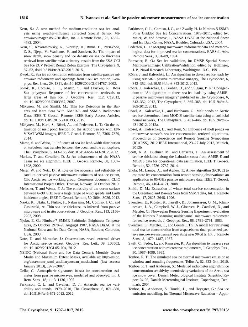
1816 N. Ivanova et al.: Satellite passive microwave measurements of sea ice concentration
Kern, S.: A new method for medium-resolution sea ice anal-
ysis using weather-influence corrected Special Sensor Mi-
crowave/Imager 85 GHz data, Int. J. Remote Sens., 25, 4555–
4582, 2004.
Kern, S., Khvorostovsky, K., Skourup, H., Rinne, E., Parsakhoo,
Z. S., Djepa, V., Wadhams, P., and Sandven, S.: The impact of
snow depth, snow density and ice density on sea ice thickness
retrieval from satellite radar altimetry: results from the ESA-CCI
Sea Ice ECV Project Round Robin Exercise, The Cryosphere, 9,
37–52, doi:10.5194/tc-9-37-2015, 2015.
Kwok, R.: Sea ice concentration estimates from satellite passive mi-
crowave radiometry and openings from SAR ice motion, Geo-
phys. Res. Lett., 29, 1311, doi:10.1029/2002GL014787, 2002.
Kwok, R., Comiso, J. C., Martin, S., and Drucker, R.: Ross
Sea polynyas: Response of ice concentration retrievals to
large areas of thin ice, J. Geophys. Res., 112, C12012,
doi:10.1029/2006JC003967, 2007.
Mäkynen, M. and Similä, M.: Thin Ice Detection in the Bar-
ents and Kara Seas With AMSR-E and SSMIS Radiometer
Data, IEEE T. Geosci. Remote, IEEE Early Access Articles,
doi:10.1109/TGRS.2015.2416393, 2015.
Mäkynen, M., Kern, S., Rösel, A., and Pedersen, L. T.: On the es-
timation of melt pond fraction on the Arctic Sea ice with EN-
VISAT WSM images, IEEE T. Geosci. Remote, 52, 7366–7379,
2014.
Marcq, S. and Weiss, J.: Influence of sea ice lead-width distribution
on turbulent heat transfer between the ocean and the atmosphere,
The Cryosphere, 6, 143–156, doi:10.5194/tc-6-143-2012, 2012.
Markus, T. and Cavalieri, D. J.: An enhancement of the NASA
Team sea ice algorithm, IEEE T. Geosci. Remote, 38, 1387–
1398, 2000.
Meier, W. and Notz, D.: A note on the accuracy and reliability of
satellite-derived passive microwave estimates of sea-ice extent,
Clic Arctic sea ice working group, Consensus document, CLIC
International Project Office, Tromsø, Norway, 28 October 2010.
Meissner, T. and Wentz, F. J.: The emissivity of the ocean surface
between 6–90 GHz over a large range of wind speeds and Earth
incidence angles, IEEE T. Geosci. Remote, 50, 3004–3026, 2012.
Naoki, K., Ukita, J., Nishio, F., Nakayama, M., Comiso, J. C., and
Gasiewski, A: Thin sea ice thickness as inferred from passive
microwave and in situ observations, J. Geophys. Res., 113, 2156–
2202, 2008.
Njoku, E. G.: Nimbus-7 SMMR Pathfinder Brightness Tempera-
tures, 25 October 1978–20 Augugst 1987, NASA DAAC at the
National Snow and Ice Data Center, NASA, Boulder, Colorado,
USA, 2003.
Notz, D. and Marotzke, J.: Observations reveal external driver
for Arctic sea-ice retreat, Geophys. Res. Lett., 39, L08502,
doi:10.1029/2012GL051094, 2012.
NSIDC (National Snow and Ice Data Center): Monthly Ocean
Masks and Maximum Extent Masks, available at: http://nsidc.
org/data/smmr_ssmi_ancillary/ocean_masks.html (last access:
January 2013), 1979–2007.
Oelke, C.: Atmospheric signatures in sea ice concentration esti-
mates from passive microwaves: modelled and observed, Int. J.
Rem. Sens., 18, 1113–1136, 1997.
Parkinson, C. L. and Cavalieri, D. J.: Antarctic sea ice vari-
ability and trends, 1979–2010, The Cryosphere, 6, 871–880,
doi:10.5194/tc-6-871-2012, 2012.
Parkinson, C. L., Comiso, J. C., and Zwally, H. J.: Nimbus-5 ESMR
Polar Gridded Sea Ice Concentrations, 1978–2011, edited by:
Meier, W. and Stroeve, J., NASA DAAC at the National Snow
and Ice Data Center, NASA, Boulder, Colorado, USA, 2004.
Pedersen, L. T.: Merging microwave radiometer data and meteoro-
logical data for improved sea ice concentrations, EARSeL Adv.
Remote Sens., 3, 81–89, 1994.
Ramseier, R. O.: Sea ice validation, in: DMSP Special Sensor
Microwave/Imager Calibration/Validation, edited by: Hollinger,
J. P., Naval Research Laboratory, Washington, D.C., 1991.
Röhrs, J. and Kaleschke, L.: An algorithm to detect sea ice leads by
using AMSR-E passive microwave imagery, The Cryosphere, 6,
343–352, doi:10.5194/tc-6-343-2012, 2012.
Röhrs, J., Kaleschke, L., Bröhan, D., and Siligam, P. K.: Corrigen-
dum to “An algorithm to detect sea ice leads by using AMSR-
E passive microwave imagery” published in The Cryosphere, 6,
343–352, 2012, The Cryosphere, 6, 365–365, doi:10.5194/tc-6-
365-2012, 2012.
Rösel, A., Kaleschke, L., and Birnbaum, G.: Melt ponds on Arctic
sea ice determined from MODIS satellite data using an artificial
neural network, The Cryosphere, 6, 431–446, doi:10.5194/tc-6-
431-2012, 2012a.
Rösel, A., Kaleschke, L., and Kern, S.: Influence of melt ponds on
microwave sensor’s sea ice concentration retrieval algorithms,
Proceedings of Geoscience and Remote Sensing Symposium
(IGARSS), 2012 IEEE International, 23–27 July 2012, Munich,
2012b.
Scott, K. A., Buehner, M., and Carrieres, T.: An assessment of
sea-ice thickness along the Labrador coast from AMSR-E and
MODIS data for operational data assimilation, IEEE T. Geosci.
Remote, 52, 2726–2737, 2014.
Shokr, M., Lambe, A., and Agnew, T.: A new algorithm (ECICE) to
estimate ice concentration from remote sensing observations: an
application to 85-GHz passive microwave data, IEEE T. Geosci.
Remote, 46, 4104–4121, 2008.
Smith, D. M.: Extraction of winter total sea-ice concentration in
the Greenland and Barents Seas from SSM/I data, Int. J. Remote
Sens., 17, 2625–2646, 1996.
Svendsen, E., Kloster, K., Farrelly, B., Johannessen, O. M., Johan-
nessen, J. A., Campbell, W. J., Gloersen, P., Cavalieri, D., and
Matzler, C.: Norwegian Remote Sensing Experiment, evaluation
of the Nimbus 7 scanning multichannel microwave radiometer
for sea ice research, J. Geophys. Res., 88, 2781–2791, 1983.
Svendsen, E., Matzler, C., and Grenfell, Th.: A model for retrieving
total sea ice concentration from a spaceborne dual-polarized pas-
sive microwave instrument operating near 90 GHz, Int. J. Remote
Sens., 8, 1479–1487, 1987.
Swift, C., Fedor, L., and Ramseier, R.: An algorithm to measure sea
ice concentration with microwave radiometers, J. Geophys. Res.,
90, 1087–1099, 1985.
Tonboe, R. T.: The simulated sea ice thermal microwave emission at
window and sounding frequencies, Tellus A, 62, 333–344, 2010.
Tonboe, R. T. and Andersen, S.: Modelled radiometer algorithm ice
concentration sensitivity to emissivity variations of the Arctic sea
ice snow cover, Danish Meteorological Institute Scientific Re-
port 04-03, Danish Meteorological Institute, Copenhagen, Den-
mark, 2004.
Tonboe, R., Andersen, S., Toudal, L., and Heygster, G.: Sea ice
emission modelling, in: Thermal Microwave Radiation – Appli-
The Cryosphere, 9, 1797–1817, 2015 www.the-cryosphere.net/9/1797/2015/

N. Ivanova et al.: Satellite passive microwave measurements of sea ice concentration 1817
cations for Remote Sensing, edited by: Mätzler, C., Rosenkranz,
P. W., Battaglia, A., and Wigneron, J. P., IET Electromagnetic
Waves Series 52, London, UK, 2006.
Tonboe, R. T., Dybkjær, G., and Høyer, J. L.: Simulations of the
snow covered sea ice surface temperature and microwave effec-
tive temperature, Tellus A, 63, 1028–1037, 2011.
Tschudi, M. A., Maslanik, J. A., and Perovich, D. K.: Derivation of
melt pond coverage on arctic sea ice using MODIS observation,
Remote Sens. Environ., 112, 2605–2614, 2008.
Ulaby, F. T., Moore, R. K., and Fung, A. K.: Microwave Remote
Sensing. Active and Passive, Norwood, MA: Artech House Inc,
1986.
Wentz, F. J.: A well-calibrated ocean algorithm for SSM/I, J. Geo-
phys. Res., 102, 8703–8718, 1997.
Wentz, F. J., Ricciardulli, L., Hilburn, K. A., and Mears, C. A.: How
much more rain will global warming bring?, Science, 317, 233–
235, 2007.
Wiesmann, A. and Mätzler, C.: Microwave emission model of lay-
ered snowpacks, Remote Sens. Environ., 70, 307–316, 1999.
Willmes, S., Nicolaus, M., and Haas, C.: The microwave emissiv-
ity variability of snow covered first-year sea ice from late winter
to early summer: a model study, The Cryosphere, 8, 891–904,
doi:10.5194/tc-8-891-2014, 2014.
www.the-cryosphere.net/9/1797/2015/ The Cryosphere, 9, 1797–1817, 2015