Embed Size (px)
Citation preview

Interacting Fermions Approach to 2D Critical Models
Pierluigi Falco
Institute for Advanced StudySchool of Mathematics
Pierluigi Falco Interacting Fermions Approach to 2D Critical Models

Outline
• (Brief) Introduction on Ising model and Onsager’s exact solution.
• Definitions of the Eight-Vertex and Ashkin-Teller models.
• Qualitative discussion of the critical properties.
• List of rigorous results.
• Open problems.
Pierluigi Falco Interacting Fermions Approach to 2D Critical Models

Ising Model
Configuration: Place +1 or −1 at each site of Λ
σ = {σx = ±1 | x ∈ Λ}
Energy: given J (positive for definiteness)
H(σ) = −J∑x∈Λj=0,1
σxσx+ej
Probability: given the inverse temperature β ≥ 0
P(σ) =1
Z(Λ, β)e−βH(σ) Z(Λ, β) =
∑σ
e−βH(σ)
Pierluigi Falco Interacting Fermions Approach to 2D Critical Models

Ising Model
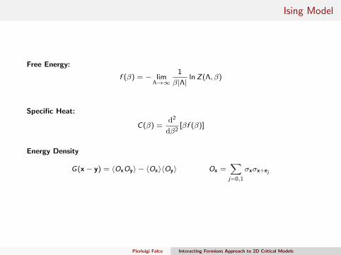
Free Energy:
f (β) = − limΛ→∞
1
β|Λ|lnZ(Λ, β)
Specific Heat:
C(β) =d2
dβ2[βf (β)]
Energy Density
G(x− y) = 〈OxOy〉 − 〈Ox〉〈Oy〉 Ox =∑j=0,1
σxσx+ej
Pierluigi Falco Interacting Fermions Approach to 2D Critical Models

Ising Model
Free Energy:
f (β) = − limΛ→∞
1
β|Λ|lnZ(Λ, β)
Specific Heat:
C(β) =d2
dβ2[βf (β)]
Energy Density
G(x− y) = 〈OxOy〉 − 〈Ox〉〈Oy〉 Ox =∑j=0,1
σxσx+ej
Pierluigi Falco Interacting Fermions Approach to 2D Critical Models
Ising Model
Free Energy:
f (β) = − limΛ→∞
1
β|Λ|lnZ(Λ, β)
Specific Heat:
C(β) =d2
dβ2[βf (β)]
Energy Density
G(x− y) = 〈OxOy〉 − 〈Ox〉〈Oy〉 Ox =∑j=0,1
σxσx+ej
Pierluigi Falco Interacting Fermions Approach to 2D Critical Models

Ising Model
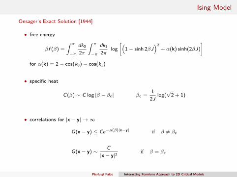
Onsager’s Exact Solution [1944]
• free energy
βf (β) =
∫ π
−π
dk0
2π
∫ π
−π
dk1
2πlog
[(1− sinh 2βJ
)2+ α(k) sinh(2βJ)
]for α(k) = 2− cos(k0)− cos(k1)
• specific heat
C(β) ∼ C log |β − βc | βc =1
2Jlog(√
2 + 1)
• correlations for |x− y| → ∞
G(x− y) ≤ Ce−µ(β)|x−y| if β 6= βc
G(x− y) ∼C
|x− y|2if β = βc
Pierluigi Falco Interacting Fermions Approach to 2D Critical Models

Ising Model
Onsager’s Exact Solution [1944]
• free energy
βf (β) =
∫ π
−π
dk0
2π
∫ π
−π
dk1
2πlog
[(1− sinh 2βJ
)2+ α(k) sinh(2βJ)
]for α(k) = 2− cos(k0)− cos(k1)
• specific heat
C(β) ∼ C log |β − βc | βc =1
2Jlog(√
2 + 1)
• correlations for |x− y| → ∞
G(x− y) ≤ Ce−µ(β)|x−y| if β 6= βc
G(x− y) ∼C
|x− y|2if β = βc
Pierluigi Falco Interacting Fermions Approach to 2D Critical Models

Meaning of Onsager’s construction
Grassmann Algebra [=Fermions] ψ1, . . . , ψn such that
ψiψj = −ψjψi
for i1 < i2 < · · · < iq∫dψj ψi1 · · ·ψipψjψip+2
· · ·ψiq = (−1)pψi1 · · ·ψipψip+2· · ·ψiq∫
dψj [no ψj ] = 0
Grassmann Gaussian Integral Two sets of Grassmann variables, ψ1, · · · , ψn andψ1, · · · , ψn ∫
dψ1dψ1 · · · dψndψn exp{∑
i,j
ψiMijψj
}= det(M)
Onsager’s construction [...actually Kasteleyn’s] Two sets of 2|Λ| Grassmann variables,
Z(Λ, β) = detM =
∫DψDψ exp
{ ∑α,β=1,2
∑i,j∈Λ
ψα,iMαβij ψβ,j
}Ising model= system of free fermions
Pierluigi Falco Interacting Fermions Approach to 2D Critical Models

Meaning of Onsager’s construction
Grassmann Algebra [=Fermions] ψ1, . . . , ψn such that
ψiψj = −ψjψi
for i1 < i2 < · · · < iq∫dψj ψi1 · · ·ψipψjψip+2
· · ·ψiq = (−1)pψi1 · · ·ψipψip+2· · ·ψiq∫
dψj [no ψj ] = 0
Grassmann Gaussian Integral Two sets of Grassmann variables, ψ1, · · · , ψn andψ1, · · · , ψn ∫
dψ1dψ1 · · · dψndψn exp{∑
i,j
ψiMijψj
}= det(M)
Onsager’s construction [...actually Kasteleyn’s] Two sets of 2|Λ| Grassmann variables,
Z(Λ, β) = detM =
∫DψDψ exp
{ ∑α,β=1,2
∑i,j∈Λ
ψα,iMαβij ψβ,j
}
Ising model= system of free fermions
Pierluigi Falco Interacting Fermions Approach to 2D Critical Models

Meaning of Onsager’s construction
Grassmann Algebra [=Fermions] ψ1, . . . , ψn such that
ψiψj = −ψjψi
for i1 < i2 < · · · < iq∫dψj ψi1 · · ·ψipψjψip+2
· · ·ψiq = (−1)pψi1 · · ·ψipψip+2· · ·ψiq∫
dψj [no ψj ] = 0
Grassmann Gaussian Integral Two sets of Grassmann variables, ψ1, · · · , ψn andψ1, · · · , ψn ∫
dψ1dψ1 · · · dψndψn exp{∑
i,j
ψiMijψj
}= det(M)
Onsager’s construction [...actually Kasteleyn’s] Two sets of 2|Λ| Grassmann variables,
Z(Λ, β) = detM =
∫DψDψ exp
{ ∑α,β=1,2
∑i,j∈Λ
ψα,iMαβij ψβ,j
}Ising model= system of free fermions
Pierluigi Falco Interacting Fermions Approach to 2D Critical Models

Eight Vertex Model
Sutherland (1970),Fan and Wu (1970):
Draw arrows on the edges of atwo-dimensional square lattice, with therestriction that an even number ofarrows points into every vertex.
Pierluigi Falco Interacting Fermions Approach to 2D Critical Models

Eight Vertex Model
Sutherland (1970),Fan and Wu (1970):
Draw arrows on the edges of atwo-dimensional square lattice, with therestriction that an even number ofarrows points into every vertex.
Pierluigi Falco Interacting Fermions Approach to 2D Critical Models

Eight Vertex Model
8 possible arrangements of arrows at a site.
E EE
E E
1 2
3 4
Assign four possible energies (’zero field’ case).
Total EnergyH(ω) = E1n1(ω) + E2n2(ω) + E3n3(ω) + E4n4(ω)
Pierluigi Falco Interacting Fermions Approach to 2D Critical Models

Eight Vertex Model
8 possible arrangements of arrows at a site.
Assign four possible energies (’zero field’ case).
Total EnergyH(ω) = E1n1(ω) + E2n2(ω) + E3n3(ω) + E4n4(ω)
Pierluigi Falco Interacting Fermions Approach to 2D Critical Models

Eight Vertex Model
8 possible arrangements of arrows at a site.
Assign four possible energies (’zero field’ case).
Total EnergyH(ω) = E1n1(ω) + E2n2(ω) + E3n3(ω) + E4n4(ω)
Pierluigi Falco Interacting Fermions Approach to 2D Critical Models

Eight Vertex Model
8 possible arrangements of arrows at a site.
E EE
E E
1 2
3 4
Assign four possible energies (’zero field’ case).
Total EnergyH(ω) = E1n1(ω) + E2n2(ω) + E3n3(ω) + E4n4(ω)
Pierluigi Falco Interacting Fermions Approach to 2D Critical Models

Eight Vertex Model
8 possible arrangements of arrows at a site.
E EE
E E
1 2
3 4
Assign four possible energies (’zero field’ case).
Total EnergyH(ω) = E1n1(ω) + E2n2(ω) + E3n3(ω) + E4n4(ω)
Pierluigi Falco Interacting Fermions Approach to 2D Critical Models

Ashkin-Teller Model
Ashkin and Teller (1943)
Place a label A,B,C or D to each siteof two-dimensional square lattice.
D A B A
C B A B
D A C C
D A B B
Pierluigi Falco Interacting Fermions Approach to 2D Critical Models

Ashkin-Teller Model
Ashkin and Teller (1943)
Place a label A,B,C or D to each siteof two-dimensional square lattice.
D A B A
C B A B
D A C C
D A B B
Pierluigi Falco Interacting Fermions Approach to 2D Critical Models

Ashkin-Teller Model
10 possible non oriented arrangements of labels at an edge.
A A
B B
E1
C C
D D A D
E2
B C
A C
E3
B D A B
E4
C D
Assign four different energies (case E2 = E3 = E4 6= E1 is ’4 States Potts Model’)
Total EnergyH(ω) = E1n1(ω) + E2n2(ω) + E3n3(ω) + E4n4(ω)
Pierluigi Falco Interacting Fermions Approach to 2D Critical Models

Ashkin-Teller Model
10 possible non oriented arrangements of labels at an edge.
A A
B B
C C
D D A D B C
A C B D A B C D
Assign four different energies
(case E2 = E3 = E4 6= E1 is ’4 States Potts Model’)
Total EnergyH(ω) = E1n1(ω) + E2n2(ω) + E3n3(ω) + E4n4(ω)
Pierluigi Falco Interacting Fermions Approach to 2D Critical Models

Ashkin-Teller Model
10 possible non oriented arrangements of labels at an edge.
A A
B B
E1
C C
D D A D
E2
B C
A C
E3
B D A B
E4
C D
Assign four different energies (case E2 = E3 = E4 6= E1 is ’4 States Potts Model’)
Total EnergyH(ω) = E1n1(ω) + E2n2(ω) + E3n3(ω) + E4n4(ω)
Pierluigi Falco Interacting Fermions Approach to 2D Critical Models

Ashkin-Teller Model
10 possible non oriented arrangements of labels at an edge.
A A
B B
E1
C C
D D A D
E2
B C
A C
E3
B D A B
E4
C D
Assign four different energies (case E2 = E3 = E4 6= E1 is ’4 States Potts Model’)
Total EnergyH(ω) = E1n1(ω) + E2n2(ω) + E3n3(ω) + E4n4(ω)
Pierluigi Falco Interacting Fermions Approach to 2D Critical Models

8V and AT
In both models
H(ω) = E1n1(ω) + E2n2(ω) + E3n3(ω) + E4n4(ω)
Probability of a configuration ω, given inverse temperature, β ≥ 0,
P(ω) =1
Ze−βH(ω) Z =
∑ω
e−βH(ω)
• Without loss of generality, assume E1 + E2 + E3 + E4 = 0i.e. the independent parameters are 3.
• 8V and AT belong to a bigger class, the double Ising Models:(more intuitive qualitative analysis)
Pierluigi Falco Interacting Fermions Approach to 2D Critical Models

Double Ising Model
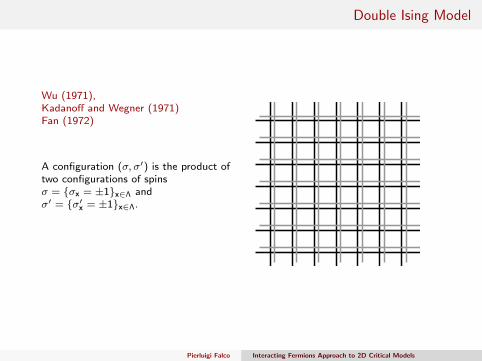
Wu (1971),Kadanoff and Wegner (1971)Fan (1972)
A configuration (σ, σ′) is the product oftwo configurations of spinsσ = {σx = ±1}x∈Λ andσ′ = {σ′x = ±1}x∈Λ.
Pierluigi Falco Interacting Fermions Approach to 2D Critical Models
Double Ising Model
Wu (1971),Kadanoff and Wegner (1971)Fan (1972)
A configuration (σ, σ′) is the product oftwo configurations of spinsσ = {σx = ±1}x∈Λ andσ′ = {σ′x = ±1}x∈Λ.
Pierluigi Falco Interacting Fermions Approach to 2D Critical Models

Double Ising Models
The energy of (σ, σ′) is function of J, J′ and J4
H(σ, σ′) = −J∑x∈Λj=0,1
σxσx+ej − J′∑x∈Λj=0,1
σ′xσ′x+ej− J4V (σ, σ′)
where V quartic in σ and σ′:
V (σ, σ′) =∑x∈Λj=0,1
∑x′∈Λj′=0,1
vj−j′ (x− x′)σxσx+ej σ′x′σ′x′+ej′
for vj (x) a lattice function such that |vj (x)| ≤ ce−κ|x|.
Probability of a configuration (σ, σ′)
P(σ, σ′) =1
Ze−βH(σ,σ′) Z =
∑σ,σ′
e−βH(σ,σ′)
Pierluigi Falco Interacting Fermions Approach to 2D Critical Models

Double Ising Models
The 8V and AT models are equivalent to a doubled Ising model if:
E1 = −J − J′ − J4 E2 = J + J′ − J4
E3 = J − J′ + J4 E4 = −J + J′ + J4
8V : V (σ, σ′) =∑x∈Λj=0,1
σx+e0σx+j(e0+e1)σ′x+e1
σ′x+j(e0+e1)
AT : V (σ, σ′) =∑x∈Λj=0,1
σxσx+ej σ′xσ′x+ej
8V AT
Pierluigi Falco Interacting Fermions Approach to 2D Critical Models

Double Ising Models
Free energy
f (β) = − limΛ→∞
1
β|Λ|lnZ(Λ, β)
Specific Heat:
C(β) =d2
dβ2[βf (β)]
Energy Density - Crossover
Gε(x− y) = 〈Oεx Oεy 〉 − 〈Oεx 〉〈Oεy 〉
where
O+x =
∑j=0,1
σxσx+ej +∑j=0,1
σ′xσ′x+ej
O−x =∑j=0,1
σxσx+ej −∑j=0,1
σ′xσ′x+ej
Pierluigi Falco Interacting Fermions Approach to 2D Critical Models

Double Ising Models
Typical case: µ(β) > 0
|Gε(x− y)| ≤ Ce−µ(β)|x−y| , |C(β)| <∞
(inverse) critical temperature βc s.t. µ(βc ) = 0, then:
• algebraic decay of correlations
Gε(x− y) ∼C
1 + |x− y|2xε, |C(β)| =∞
and x+ and x− are the energy and crossover critical exponents
• µ(β) ∼ C |β − βc |ν and ν > 0 is the correlation-length critical exponent
• C(β) ∼ C |β − βc |−α and α > 0 is the specific heat critical exponent
Finally we have four critical exponents:
x+ x− ν α
Pierluigi Falco Interacting Fermions Approach to 2D Critical Models
Qualitative Discussion
Assume for definiteness J, J′ > 0
H(σ, σ′) = −J∑x∈Λj=0,1
σxσx+ej − J′∑x∈Λj=0,1
σ′xσ′x+ej
• for J 6= J′, J4 = 0: two critical temperatures,
βc =1
2Jln(√
2 + 1) β′c =1
2J′ln(√
2 + 1)
critical exponentsx+ = x− = 1
Pierluigi Falco Interacting Fermions Approach to 2D Critical Models

Qualitative Discussion
Assume for definiteness J, J′ > 0;
H(σ, σ′) = −J∑x∈Λj=0,1
σxσx+ej − J′∑x∈Λj=0,1
σ′xσ′x+ej− J4V (σ, σ′)
• for J 6= J′, J4 = 0: two critical temperatures,
βc =1
2Jln(√
2 + 1) β′c =1
2J′ln(√
2 + 1)
critical exponentsx+ = x− = 1
• for 0 < |J4| << |J − J′|: two critical temperatures, for λ = J4/J and λ′ = J4/J′
βc =1
2Jln(√
2 + 1) + O(λ, λ′) β′c =1
2J′ln(√
2 + 1) + O(λ, λ′)
critical exponentsx+ = x− = 1
[universality]
Pierluigi Falco Interacting Fermions Approach to 2D Critical Models

Qualitative Discussion
Assume for definiteness J > 0
H(σ, σ′) = −J∑x∈Λj=0,1
σxσx+ej − J∑x∈Λj=0,1
σ′xσ′x+ej
• for J = J′, J4 = 0: one critical temperature,
βc =1
2Jln(√
2 + 1)
critical exponentsx+ = x− = 1
Pierluigi Falco Interacting Fermions Approach to 2D Critical Models

Qualitative Discussion
Assume for definiteness J > 0
H(σ, σ′) = −J∑x∈Λj=0,1
σxσx+ej − J∑x∈Λj=0,1
σ′xσ′x+ej
• for J = J′, J4 = 0: one critical temperature,
βc =1
2Jln(√
2 + 1)
critical exponentsx+ = x− = 1
Pierluigi Falco Interacting Fermions Approach to 2D Critical Models

Qualitative Discussion
Assume for definiteness J > 0
H(σ, σ′) = −J∑x∈Λj=0,1
σxσx+ej − J∑x∈Λj=0,1
σ′xσ′x+ej− J4V (σ, σ′)
• for J = J′, J4 = 0: one critical temperature,
βc =1
2Jln(√
2 + 1)
critical exponentsx+ = x− = 1
• for 0 < |J4| << J: one critical temperature, for λ = J4/J
βc =1
2Jln(√
2 + 1) + O(λ)
critical exponents
x+ = 1 + X+(λ) x− = 1 + X−(λ)
[non-universality]
Pierluigi Falco Interacting Fermions Approach to 2D Critical Models

Qualitative Discussion
For |J′ − J| → 0,|β1,c − β2,c | ∼ |J − J′|xT
A 5◦ index, the transition index xT . Then we have 5 critical exponents:
x+(λ) x−(λ) ν(λ) α(λ) xT (λ)
Pierluigi Falco Interacting Fermions Approach to 2D Critical Models

Qualitative Discussion
Motivation:
• When critical indexes are model-independent, they can be compared withexperiments.
u. class ν νth α αth
Rb2C0F4 Ising .99±.04 1 0(log)K2C0F4 Ising .97±.04 1 0(log)
4He/graphite Potts-3 .36±.03 .33...H2/graphite Potts-3 .36±.05 .33...H/Ni (111) Potts-4 .68±.07 .66...
PVA SAW .79±.01 .75PMMA θ-SAW .56±.01 .57...
3-MP-NE 3D Ising .625±.003 .630±.002SF6 3D Ising .11±.03 .110±.0034He 3D XY .6702±.0002 .669±.001
• In 8V and AT critical exponents are model-dependent: still a weak form ofuniversality is retained: some universal formulas have been conjectured for thesenonuniversal indexes.
Pierluigi Falco Interacting Fermions Approach to 2D Critical Models

Universal formulas
Kadanoff and Wegner (1971)Luther and Peschel (1975)
dν = 2− α ν =1
2− x+
Widom scaling relations: valid at criticality for any model in any dimension < 4;they don’t characterize classes of models
Pierluigi Falco Interacting Fermions Approach to 2D Critical Models

Universal formulas
Kadanoff and Wegner (1971)Luther and Peschel (1975)
dν = 2− α ν =1
2− x+
Widom scaling relations: valid at criticality for any model in any dimension < 4;they don’t characterize classes of models
Pierluigi Falco Interacting Fermions Approach to 2D Critical Models

Universal formulas
Kadanoff (1977)
x+ x− = 1
Extended scaling relation: characterize models with scaling limit given by ThirringModel
Pierluigi Falco Interacting Fermions Approach to 2D Critical Models

Universal formulas
Kadanoff (1977)
x+ x− = 1
Extended scaling relation: characterize models with scaling limit given by ThirringModel
Pierluigi Falco Interacting Fermions Approach to 2D Critical Models

Thirring model
Thirring model (Thirring 1955) is a toy model of interacting, 2-dimensional, fermion,quantum field theory. The Action is∫
dx ψx 6∂ψx + λ
∫dx (ψxψx)2
for
ψx = (ψ1,x, ψ2,x) ψx =
(ψ1,x
ψ2,x
)6∂ = 2× 2matrix
From the formal explicit solution of the Thirring model (Klaiber 1967, Hagen 1967)
xTh+ =1− λ
4π
1 + λ4π
xTh− =1 + λ
4π
1− λ4π
Pierluigi Falco Interacting Fermions Approach to 2D Critical Models

Rigorous Results
Pierluigi Falco Interacting Fermions Approach to 2D Critical Models

Rigorous results: Exact Solutions
Lieb (1967), Sutherland (1967)
• f (β), βc and α for 6V.By-product: f (βc ) and α for AT
Baxter (1971)
• f (β), βc and α for 8V
• interfacial-tension critical index.
Johnson, Krinsky and McCoy (1972)
• ν (which does satisfy 2ν = 2− α)
No exact solution for x+, x−, xT ; no exact solution for other Double Ising models.
Pierluigi Falco Interacting Fermions Approach to 2D Critical Models

Rigorous results: RG
Spencer, Pinson and Spencer (2000)
Ising model with finite range (even) perturbation:
H(σ) = −J∑x∈Λj=0,1
σxσx+ej − J4V (σ)
If ε = J4/J
• x+ = 1 for ε small enough.
Method of the proof:
– Functional integral representation of the Ising model
Z(Λ, β) =
∫DψDψ exp
{∑ψMψ + λ
∑(ψ∂ψ)2
}λ ∼ J4/J
– Renormalization group approach for computing x+.based on RG approach for fermion system Feldman, Knorrer, Trubowitz, (1998)
Pierluigi Falco Interacting Fermions Approach to 2D Critical Models

Rigorous results: RG
Mastropietro (2004)
Double Ising: for J′ = J and J4/J small enough
• convergent power series for βc (J4/J)
• convergent power series for ν(J4/J) and x+(J4/J).
Giuliani and Mastropietro (2005)
Double Ising: for J 6= J′ and J4/J, J4/J′ small enough
• convergent power series for βc (J4/J, J4/J′) and β′c (J4/J, J4/J′)
• convergent power series for xT (J4/J) [First time the index xT was introduced]
based on RG approach for system with ’vanishing beta function’ Benfatto, Gallavotti, Procacci, Scoppola (1994);
review of last three results in the book Mastropietro 2006
Above power series are convergent but no explicit formulas: not useful for extendedscaling formula.
Pierluigi Falco Interacting Fermions Approach to 2D Critical Models

Rigorous results
Benfatto, Falco, Mastropietro (2007), (2009)
Thirring model for |λ| small enough:
• Existence of the theory (in the sense of the Osterwalder-Schrader)
• Proof of Hagen and Klaiber’s formula for correlations.
There was already an axiomatic proof of the existence of the interacting theory: not good for scaling limit
Benfatto, Falco, Mastropietro (2009)
Double Ising model: for J4/J small enough
• proof of the universal formulas
2ν = 2− α ν =1
2− x+x+ x− = 1
• a new scaling relation for the index xT
xT =2− x+
2− x−
Similar results for the XYZ quantum chain
Pierluigi Falco Interacting Fermions Approach to 2D Critical Models

Idea of the proof: RG approach
Multi-scale decomposition:
Z =
∫dP(ψ) eλV (ψ) = E
[eλV (ψ)
]= lim
h→−∞Eh ◦ Eh+1 · · ·E−1 ◦ E0
[eλV (ψh+···+ψ−1+ψ0)
]where ψh, . . . , ψ−1, ψ0 are i.r.v. and
Ej [ψj,xψj,y] = Γj (x− y) with |∂mΓj (x)| ≤ γmjCecγj |x|
Define
eλ−1V (ϕ)+R−1(ϕ) = E0
[eλV (ϕ+ψ0)
]eλ−2V (ϕ)+R−2(ϕ) = E−1
[eλ−1V (ϕ+ψ−1)+R−1(ϕ+ψ−1)
]· · ·
eλjV (ϕ)+Rj (ϕ) = Ej+1
[eλj+1V (ϕ+ψj+1)+Rj+1(ϕ+ψj+1)
]· · ·
In correspondence there is a sequence of effective couplings
λh, λh+1, . . . , λ−1, λ
Pierluigi Falco Interacting Fermions Approach to 2D Critical Models

Scaling limit and RG
The flow of the effective coupling λj is
0-5-10-15...
lattice model
The crucial fact is that, given λ = J4/J, it is possible to choose λTh such that
λ−∞ = λTh−∞
Thereforexε(λ) = xThε (λTh) ε = ±
Pierluigi Falco Interacting Fermions Approach to 2D Critical Models

Scaling limit and RG
The flow of the effective coupling λj is
0-5-10-15...
lattice model
The crucial fact is that, given λ = J4/J, it is possible to choose λTh such that
λ−∞ = λTh−∞
Thereforexε(λ) = xThε (λTh) ε = ±
Pierluigi Falco Interacting Fermions Approach to 2D Critical Models

Scaling limit and RG
The flow of the effective coupling λj is
N...1050-5-10-15...
lattice modelThirring model
The crucial fact is that, given λ = J4/J, it is possible to choose λTh such that
λ−∞ = λTh−∞
Thereforexε(λ) = xThε (λTh) ε = ±
Pierluigi Falco Interacting Fermions Approach to 2D Critical Models

Non-universality
The connection with experiments is the following:
• Threshold in J4/J for the Kadanoff law: no numerical simulation (but there aresimulations of other exponents...)
• Connection with real laboratory experiments [Se/Ni (100)]? No experimentalverification of Kadanoff law.
Pierluigi Falco Interacting Fermions Approach to 2D Critical Models

Conclusions and Open Problems
model lattice scaling limit
Ising free fermions free fermions
Ising + n.n.n. interacting fermions free fermions
8V, AT, XYZ interacting fermions Thirring
in preparation:
(1 + 1)D Hubbard interacting fermions SU(2) Thirring
Open problems:
• Interacting dimers / 6V Modelnumerical simulations in Alet, Ikhlef, Jacobsen, Misguich, Pasquier (2006)
• Four Coupled Ising / Two Coupled 8V
• q−States Potts / Completely Packed Loop /...
• Spin-Spin Correlation in Ising / Other Kadanoff Formula
Pierluigi Falco Interacting Fermions Approach to 2D Critical Models