Interactive Change Point DetectionApproaches in Time-Series

A comparative study of two algorithm approaches,with real world application

Rebecca Gedda

Supervisors: Larisa Beilina & Ruomu Tan

Department of Mathematical SciencesChalmers University of Technology

In cooperation with ABB Corporate Research Centre, Germany

Mannheim, Germany, 2021

This is a Thesis for M.Sc. Degree in

Engineering Mathematics and Computational Science

at Chalmers University of Technology.

Interactive Change Point Detection Approaches in Time-Series

A comparative study of two algorithm approaches, for offline change point detection,

based on optimisation problem formulation and Bayesian statistics, with real world ap-

plication.

Rebecca Gedda

Department of Mathematical SciencesChalmers University of TechnologySE-412 96 GothenburgSwedenTelephone + 46 (0)31-772 1000

Presented and defended on: 11th May, 2021

i

Abstract

Change point detection becomes more and more important as datasetsincrease in size, where unsupervised detection algorithms can help usersprocess data. This is of importance for datasets where multiple phasesare present and need to be separated in order to be compared. To detectchange points, a number of unsupervised algorithms have been developedwhich are based on different principles. One approach is to define an op-timisation problem and minimise a cost function along with a penaltyfunction. Another approach uses Bayesian statistics to predict the prob-ability of a specific point being a change point. This study examineshow the algorithms are affected by features in the data, and the possi-bility to incorporate user feedback and a priori knowledge about the data.

The optimisation and Bayesian approaches for offline change point de-tection are studied and applied to simulated datasets as well as a realworld multi-phase dataset. In the optimisation approach, the choice ofthe cost function affects the predictions made by the algorithm. In exten-sion to the existing studies, a new type of cost function using Tikhonovregularisation is introduced. The Bayesian approach calculates the pos-terior distribution for the probability of time steps being a change point.It uses a priori knowledge on the distance between consecutive changepoints and a likelihood function with information about the segments.

Performance comparison in terms of accuracy of the two approaches formthe foundation of this work. The study has found that the performanceof the change point detection algorithms are affected by the features inthe data. The approaches have previously been studied separately anda novelty lies in comparing the predictions made by the two approachesin a specific setting, consisting of simulated datasets and a real worldexample.

Based on the comparison of various change point detection algorithms,several directions for future research are discussed. A potential extensionis to apply the studied concept for offline algorithms, to the correspond-ing online algorithms. The study of other cost functions can be exploredfurther, with emphasis on modified versions of the regularised cost func-tions presented in this work.

Key words: Change point detection, unsupervised machine learning, opti-misation, Bayesian statistics, Tikhonov regularisation.

ii

Contents

1 Introduction 11.1 Goal . . . . . . . . . . . . . . . . . . . . . . . . . . . . . . . . . . . . . . . . 21.2 Limitations and scope . . . . . . . . . . . . . . . . . . . . . . . . . . . . . . 2

2 Background 32.1 Notation and definition . . . . . . . . . . . . . . . . . . . . . . . . . . . . . 32.2 Optimisation approach . . . . . . . . . . . . . . . . . . . . . . . . . . . . . . 5

2.2.1 Search direction . . . . . . . . . . . . . . . . . . . . . . . . . . . . . 62.2.2 Cost functions . . . . . . . . . . . . . . . . . . . . . . . . . . . . . . 8

2.3 Bayesian approach . . . . . . . . . . . . . . . . . . . . . . . . . . . . . . . . 112.4 Methods of error estimation . . . . . . . . . . . . . . . . . . . . . . . . . . . 14

3 Method 163.1 Simulation of data . . . . . . . . . . . . . . . . . . . . . . . . . . . . . . . . 163.2 PRONTO data exploration . . . . . . . . . . . . . . . . . . . . . . . . . . . 203.3 Testing procedure . . . . . . . . . . . . . . . . . . . . . . . . . . . . . . . . . 21

4 Results 224.1 Simulated datasets . . . . . . . . . . . . . . . . . . . . . . . . . . . . . . . . 23

4.1.1 Piecewise constant data . . . . . . . . . . . . . . . . . . . . . . . . . 264.1.2 Piecewise linear data . . . . . . . . . . . . . . . . . . . . . . . . . . . 274.1.3 Changing variance . . . . . . . . . . . . . . . . . . . . . . . . . . . . 274.1.4 Autoregressive data . . . . . . . . . . . . . . . . . . . . . . . . . . . 284.1.5 Exponential decay data . . . . . . . . . . . . . . . . . . . . . . . . . 294.1.6 Oscillation decay data . . . . . . . . . . . . . . . . . . . . . . . . . . 30

4.2 Real dataset . . . . . . . . . . . . . . . . . . . . . . . . . . . . . . . . . . . . 31

5 Discussion 345.1 Testing procedure . . . . . . . . . . . . . . . . . . . . . . . . . . . . . . . . . 345.2 Test metrics . . . . . . . . . . . . . . . . . . . . . . . . . . . . . . . . . . . . 355.3 Results . . . . . . . . . . . . . . . . . . . . . . . . . . . . . . . . . . . . . . . 36

5.3.1 Simulated datasets . . . . . . . . . . . . . . . . . . . . . . . . . . . . 375.3.2 Real dataset . . . . . . . . . . . . . . . . . . . . . . . . . . . . . . . 40

5.4 User interaction . . . . . . . . . . . . . . . . . . . . . . . . . . . . . . . . . . 425.4.1 Optimisation approach . . . . . . . . . . . . . . . . . . . . . . . . . . 425.4.2 Bayesian approach . . . . . . . . . . . . . . . . . . . . . . . . . . . . 43

5.5 Future work . . . . . . . . . . . . . . . . . . . . . . . . . . . . . . . . . . . . 43

6 Conclusion 44

References 45

A Bayesian posterior distribution illustrations 48

B Code 50

iii

1 Introduction

The topic of Change Point Detection (CPD) has become more and more relevant as timeseries datasets increase in size and often contain repeated patterns. By detecting changepoints in data, segmentation can be performed to group similar phases of the time seriesdata together. This is of importance for datasets where multiple phases are present andneed to be separated in order to be compared. To detect the change points, a number ofalgorithms have been developed and are based on different principles. One approach is todefine an optimisation problem and minimise a cost function along with a penalty function.The other approach uses Bayesian statistics to predict the probability of a change pointat a specific time. The performance of algorithm and approach can vary depending onthe data at hand. This thesis explores how the mentioned approaches are affected by fea-tures in the data. For a firm application link, real world datasets are explored in the study.

The first work on change point detection was done by Page [1, 2] where piecewise identicallydistributed datasets were studied. The objective was to identify various features in theindependent and non-overlapping segments. Examples of features can be mean, varianceand distribution function for each data segment. Detection of change points can eitherbe done in real time or in retrospect, and for a single signal or in multiple dimensions.The real time approach is generally known as online detection, while the retrospectiveapproach is known as offline detection. This work is based on offline detection, meaningall data is available for the entire time interval under investigation. Many CPD algorithmsare generalised for usage on multi-dimensional data [3] where one-dimensional data canbe seen as a special case. This work focuses on one-dimensional time dependent data,where results are more intuitive and common in real world settings. Another importantassumption is connected to the number of change points in the data. This can either beknown beforehand or unknown. This work assumes that the number of change points isnot known.

Change point detection can be applied to any type of signal containing distinct segments.Various CPD methods have been applied to a vast spread of areas, stretching from sen-sor signals [4] to natural language processing [5]. Some CPD methods have also beenimplemented for financial analysis [6] and network systems [7], where the algorithms areable to detect changes in the underlying setting. In these papers, changes in stock pricesand traffic flows are studied respectively. Change point detection has also been appliedto chemical processes [8], where the change points in the mean of the data from chemicalprocesses are considered to be the representation of changed quality of production. CPDis of special interest for batch related processes, where a batch is repeated multiple timesfor production and consists for multiple phases which are of interest to identify. Thisillustrates the usability for change point detection and presents the need of domain expertknowledge. Better predictions can potentially be made if domain specific knowledge canbe incorporated into the prediction model. The domain expert can also determine if thepredictions are accurate or not.

The current work is based on numerical testing of two approaches for CPD, the opti-misation approach with and without regularisation and the Bayesian approach, applied to

1

some real world data from a multi-phase flow facility. Both approaches are developed andstudied separately in previous studies [3, 9]. Performance comparison and the evaluation ofcomputational efficiency of these approaches form the foundation of this work. The workby Truong et al. [3] gives a good overview of change point detection algorithms which arebased on the optimisation approach. In extension to the existing work, new cost func-tions based on regularisation can be implemented. Some examples where regularisationtechniques are used in machine learning algorithms are presented in [10, 11, 12]. For theBayesian approach, the work by Fearnhead [9] gives a thorough description of the mathe-matics behind the algorithm. These two approaches have been studied separately and thiswork aims to compare the predictions made by the two approaches in a specific settingof simulated data and a real world example. For comparison, the methods presented byvan den Burg and Williams [13] are used, along with metrics specified by Truong et al. [3].

This work is structured as follows: first the appropriate notation is introduced alongwith definitions. Then, the two approaches, optimisation and Bayesian, are derived sep-arately in section 2 along with the metrics used for comparison. Section 3 describes theused datasets and the testing procedure. The results of the study are presented in section4 and a discussion is held in section 5. Finally, a summary of findings and conclusions isprovided in section 6.

1.1 Goal

This work aims to present a comparison between two different algorithmic approachesused for change point detection: the optimisation approach and the Bayesian approach.The first approach introduces a functional which should be minimised while the secondapproach is based on Bayesian statistics. Throughout the work, the following two mainquestions are considered:

• How are the two change point detection approaches affected by the features of inves-tigated data?

• How can user knowledge and feedback be incorporated in the two above mentionedapproaches?

The first question formulates the main research investigation of this work and suggeststhat studied algorithms should be compared. The secondary focus of the work lies in thedomain expert interplay, where the possibility of interaction is studied.

1.2 Limitations and scope

As the study and application area of change point detection are extensive, limitations areof the essence. There are numerous algorithms and approaches which can be used foroffline change point detection, where this work focuses solely on the optimisation problemand the Bayesian statistics approach. Other methods, such as Maximum likelihood, arereviewed in [14] and are not studied in this work.

2

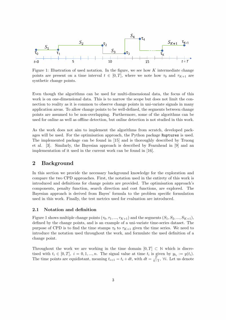
Figure 1: Illustration of used notation. In the figure, we see how K intermediate changepoints are present on a time interval t ∈ [0, T ], where we note how τ0 and τK+1 aresynthetic change points.

Even though the algorithms can be used for multi-dimensional data, the focus of thiswork is on one-dimensional data. This is to narrow the scope but does not limit the con-nection to reality as it is common to observe change points in uni-variate signals in manyapplication areas. To allow change points to be well-defined, the segments between changepoints are assumed to be non-overlapping. Furthermore, some of the algorithms can beused for online as well as offline detection, but online detection is not studied in this work.

As the work does not aim to implement the algorithms from scratch, developed pack-ages will be used. For the optimisation approach, the Python package Ruptures is used.The implemented package can be found in [15] and is thoroughly described by Truonget al. [3]. Similarly, the Bayesian approach is described by Fearnhead in [9] and animplementation of it used in the current work can be found in [16].

2 Background

In this section we provide the necessary background knowledge for the exploration andcompare the two CPD approaches. First, the notation used in the entirety of this work isintroduced and definitions for change points are provided. The optimisation approach’scomponents, penalty function, search direction and cost functions, are explored. TheBayesian approach is derived from Bayes’ formula to the problem specific formulationused in this work. Finally, the test metrics used for evaluation are introduced.

2.1 Notation and definition

Figure 1 shows multiple change points (τ0, τ1, ..., τK+1) and the segments (S1, S2, ..., SK+1),defined by the change points, and is an example of a uni-variate time-series dataset. Thepurpose of CPD is to find the time stamps τ0 to τK+1 given the time series. We need tointroduce the notation used throughout the work, and formulate the used definition of achange point.

Throughout the work we are working in the time domain [0, T ] ⊂ N which is discre-tised with ti ∈ [0, T ], i = 0, 1, ..., n. The signal value at time ti is given by yti := y(ti).The time points are equidistant, meaning ti+1 = ti + dt, with dt = T

n−1 , ∀i. Let us denote

3

the jump by [yti ] in time of the discrete function yti at time moment ti which we define as

[yti ] := lims→0+

(y(ti+s)− y(ti−s)). (1)

A set of K change points is denoted by T and is a subset of time indices {1, 2, . . . , n}. Theindividual change points are indicated as τj , with j ∈ {0, 1, . . . ,K,K + 1}, where τ0 = 0and τK+1 = T . Note, with this definition the first and final time points are implicit changepoints, and we have K intermediate change points (|T | = |{τ1, . . . , τK}| = K). A segmentof the signal from a to b is denoted as ya:b, where y0:T means the entire signal. With theintroduced notation for change points, the segment Sj between change points τj−1 and τjis defined as Sj := [τj−1, τj ], |Sj | = τj − τj−1. Sj is the j-th non-overlapping segment inthe signal, j ∈ {1, . . . ,K + 1}, see Figure 1. Note that the definition for Sj does not holdfor j = 0, since this is the first change point.

As the goal is to identify whether a change has occurred in the signal, a proper defini-tion of the term change point is needed along with clarification of change point detection.Change point detection is closely related to change point estimation (also known as changepoint mining, see [17, 18]). According to Aminikhanghahi and Cook [19], change pointestimation tries to model and interpret known changes in time series, while change pointdetection tries to identify whether a change has occurred [19]. This illustrates that we willnot focus on the change points’ characteristics, but rather if a change point exists or not.

One challenge is to identify the number of change points in a given time series. Theproblem is a balance between having enough change points whilst not over-fitting to thedata. If the number of change points is known beforehand the problem is merely a best fitproblem. On the other hand, if the number of change points is not known, the problemcan be seen as an optimisation problem with a penalty term for every added change point,or as enforcing a threshold when we are certain enough that a change point exists. Itis evident that we need clear definitions of change points in order to detect them. Thedefinitions for change point and change point detection are defined below and will be usedthroughout this work.

Definition 1 (Change point) A change point represents a transition between differentstates in a signal or dataset. If two consecutive segments ytl:ti and yti,tm, tl < ti <tm, l, i,m = 0, ..., n, defined as

ytl:ti = {tk|[y(tk)] < |εl|, l ≤ k ≤ i},yti:tm = {tk|[y(tk)] < |εm|, i ≤ k ≤ m},

(2)

have a distinct change in features such that |εl| << |εm| or |εl| >> |εm|, or if yti is alocal extreme point (i.e minimum or maximum1) then, τj = ti, j = 0, 1, ...,K,K + 1 is achange point between the two segments.

Remark: the first change point τ0 = t0 and the final change point τK+1 = tn are artificialchange points which are used to define segments. These two points are defined the same

1If f(x∗) ≤ f(x) or f(x∗) ≥ f(x) for all x in X within distance ε of x∗, then x∗ is a local extreme point.

4

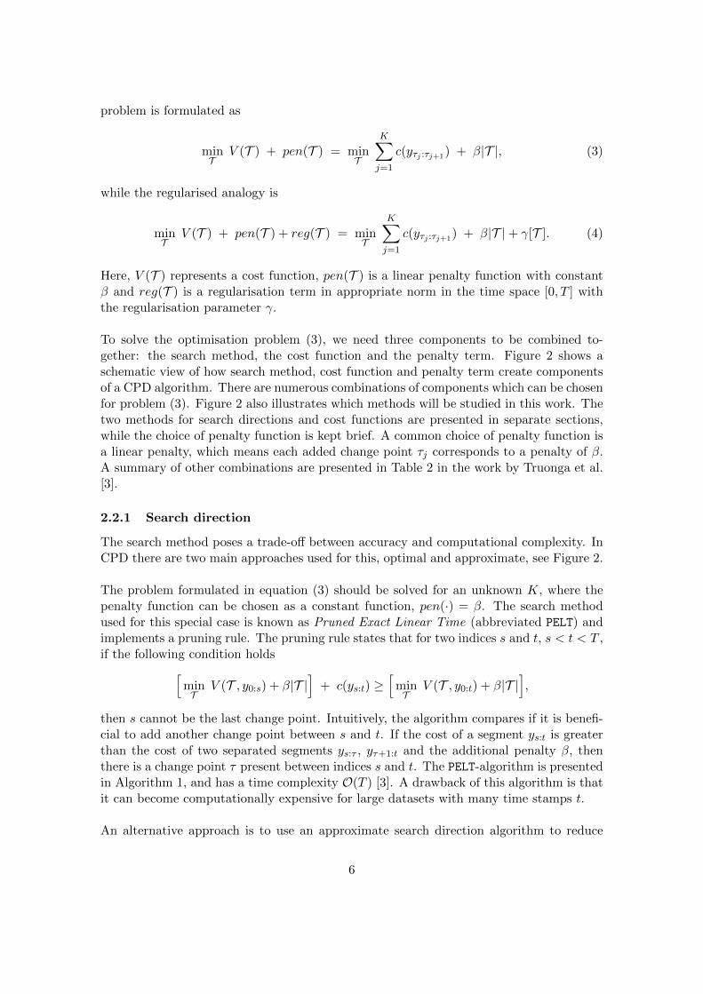
Figure 2: Illustration of the components used in the optimisation approach for changepoint detection. Each of the three components illustrate the strategies studied in thiswork.

for all predictions and are not part of the prediction process. We note that the meaningof a distinct change in this definition is different for different CPD methods, and it isdiscussed in detail in section 3. This definition is useful when dealing with features in thedata, but there may be other types of change points. These points can be more complexto identify, but are of interest for a domain expert. These change points are referred to asdomain specific change points and are defined below.

Definition 2 (Change point, domain specific) For some process data, a change pointis where a phase in the process starts or ends. These points can be indicated in the data,or be the points in the process of specific interest without a general change in data features.

Finally, we give one more definition of CPD for the case of available information aboutthe probability distribution of a stochastic process.

Definition 3 (Change point detection) Identification of times when the probabilitydistribution of a stochastic process or time series segment changes. This concerns detect-ing whether or not a change has occurred, or whether several changes might have occurred,and identifying the times of any such changes.

2.2 Optimisation approach

Solving the task of identifying change points in a time series can be done by formulatingan optimisation problem. A detailed presentation of the framework is given in the workby Truonga et al [3], while only a brief description is presented here. The purpose is toidentify all the change points, without detecting fallacious ones. Therefore, the problem isformulated as a minimisation problem, where we strive to minimise the cost of segmentsand penalty per added change point. We need this penalty since we do not know howmany change points will be presented. Mathematically, the non-regularised optimisation

5

problem is formulated as

minT

V (T ) + pen(T ) = minT

K∑j=1

c(yτj :τj+1) + β|T |, (3)

while the regularised analogy is

minT

V (T ) + pen(T ) + reg(T ) = minT

K∑j=1

c(yτj :τj+1) + β|T |+ γ[T ]. (4)

Here, V (T ) represents a cost function, pen(T ) is a linear penalty function with constantβ and reg(T ) is a regularisation term in appropriate norm in the time space [0, T ] withthe regularisation parameter γ.

To solve the optimisation problem (3), we need three components to be combined to-gether: the search method, the cost function and the penalty term. Figure 2 shows aschematic view of how search method, cost function and penalty term create componentsof a CPD algorithm. There are numerous combinations of components which can be chosenfor problem (3). Figure 2 also illustrates which methods will be studied in this work. Thetwo methods for search directions and cost functions are presented in separate sections,while the choice of penalty function is kept brief. A common choice of penalty function isa linear penalty, which means each added change point τj corresponds to a penalty of β.A summary of other combinations are presented in Table 2 in the work by Truonga et al.[3].

2.2.1 Search direction

The search method poses a trade-off between accuracy and computational complexity. InCPD there are two main approaches used for this, optimal and approximate, see Figure 2.

The problem formulated in equation (3) should be solved for an unknown K, where thepenalty function can be chosen as a constant function, pen(·) = β. The search methodused for this special case is known as Pruned Exact Linear Time (abbreviated PELT) andimplements a pruning rule. The pruning rule states that for two indices s and t, s < t < T ,if the following condition holds[

minT

V (T , y0:s) + β|T |]

+ c(ys:t) ≥[

minT

V (T , y0:t) + β|T |],

then s cannot be the last change point. Intuitively, the algorithm compares if it is benefi-cial to add another change point between s and t. If the cost of a segment ys:t is greaterthan the cost of two separated segments ys:τ , yτ+1:t and the additional penalty β, thenthere is a change point τ present between indices s and t. The PELT-algorithm is presentedin Algorithm 1, and has a time complexity O(T ) [3]. A drawback of this algorithm is thatit can become computationally expensive for large datasets with many time stamps t.

An alternative approach is to use an approximate search direction algorithm to reduce

6

Algorithm 1: PELT-algorithm

Input: Data signal y, cost function c, penalty function β.Output: List L of estimated change points indices.

Initialise: Z - An array for storing values, length (T + 1) ;Initialise: L← ∅ - An empty list for storing change point estimations ;Initialise: X ← {0} - A list of admissible indices ;

for t = 1 to T do

t← argmins∈X [Z(s) + c(ys:t) + β] ;

L(t) = [Z(t) + c(yt:t) + β] ;X ← {s ∈ X : Z(s) + c(ys:t) ≤ Z(t)} ∪ {t}

end

complexity. To reduce the number of performed calculations, an approximate search di-rection can be used, where partial detection is common. A frequently used technique isthe Window-sliding algorithm (denoted as WIN-algorithm), where the algorithm returnsan estimated change point in each iteration. Similar to the concept used in the PELT-algorithm, the value of the cost function between segments are compared. This is knownas the discrepancy between segments and is defined as

Disc(yt−w:t, yt:t+w) = c(yt−w:t+w)−(c(yt−w:t) + c(yt:t+w)

),

where w is defined as half of the window width. Intuitively, this is merely the reduced costof adding a change point at t in the middle of the window. The discrepancy is calculatedfor all w ≤ t ≤ T −w. When all calculations are done, the peaks of the discrepancy valuesare selected as the most profitable change points. The algorithm is provided in Algorithm2. There are other approximate search directions, which are not covered in this work,presented by Trounga et al. [3]. For this work, the PELT-algorithm is used for the optimalapproach and the WIN-algorithm is used for the approximate approach.

Algorithm 2: WIN-algorithm

Input: Data signal y, cost function c, window width w, penalty function β.Output: List L of estimated change points indices.

Initialise: Z - An array for storing values, length T ;Initialise: L← ∅ - An empty list for storing change point estimations ;

for t = w to T − w dop← (t− w), . . . , t ;q ← t, . . . , (t+ w) ;r ← (t− w), . . . , (t+ w) ;Z(t)← c(yr)− [c(yp) + c(yq)] ;

endL← Peaks(Z) ;

7

2.2.2 Cost functions

The cost function can decide which feature changes are detected in the data. In otherwords, the cost function measures the homogeneity. There are two approaches for defininga cost function; parametric and non-parametric. The respective approaches assume eitherthat there is an underlying distribution in the data, or that there is no distribution in thedata. This work focuses on the parametric cost functions, for three sub-techniques illus-trated in Figure 2. The three techniques, maximum likelihood estimation, linear regressionand regularisation, are introduced in later sections with corresponding cost function defi-nitions.

Maximum Likelihood Estimation (MLE) is a powerful tool with a wide application areain statics. MLE finds the values of the model parameters that maximise the likelihoodfunction f(y|Θ) over the parameter space Θ such that

MLE(y) = maxΘ∈Θ

f(y|Θ),

where y is observed data and Θ ∈ Θ is a vector of parameters. In the setting of changepoint detection, we assume the samples are independent random variables, linked to thedistribution of a segment. This means that for all t ∈ [0, T ], the sample

yt ∼K∑j=0

f(·|θj) 1(τj < t < τj+1), (5)

where θj is a segment specific parameter for the distribution. The function 1(·) is the deltafunction δ([τj , τj+1]), and is equal to one if sample yt belongs to segment j, otherwise zero:

1(τj < t < τj+1) := δ([τj , τj+1]) =

{1 if yt ∈ [τj , τj+1],0 elsewhere.

The function f(·|θj) in (5) represents the likelihood function for the distribution withparameter θj . Then the MLE(yt) reads:

MLE(yt) = maxθj∈Θ

K∑j=0

f(·|θj) 1(τj < t < τj+1)

where θj is segment specific parameter for the distribution. Using MLE(yt) we can es-timate the segment parameters θj , which are the features in the data that change at thechange points. If the distribution family of f is known and the sum of costs, V in (3) or(4), is equal to the negative log-likelihood of f , then MLE is equivalent to change pointdetection. Generally, the distribution f is not known, and therefore the cost functioncannot be defined as the negative log-likelihood of f .

In some datasets, we can assume the segments to follow a Gaussian distribution, withparameters mean and variance. More precisely, if f is a Gaussian distribution, the MLEfor expected value (which is the distribution mean) is the sample mean. If we want toidentify a shift in the mean between segments, but where the variance is constant, the

8

cost function can be defined as the quadratic error between a sample and the MLE of themean. For a sample yt and the segment mean ya:b the cost function is defined as

cL2(ya:b) :=

b∑t=a+1

||yt − ya:b||22, (6)

where the norm ‖ · ‖2 is the usual L2-norm defined for any vector v ∈ Rn as

‖v‖2 :=√

(v1)2 + (v2)2 + · · ·+ (vn)2.

The cost function (6) can be simplified for uni-variate signals to

cL2(ya:b) :=

b∑t=a+1

(yt − ya:b)2

which is equal to the MLE variance times length of the segment. More explicitly, for thepresumed Gaussian distribution f the MLE of the segment variance σ2

a:b is calculated as

σ2a:b = cL2(ya:b)

b−a , using the MLE of the segment mean, ya:b. This estimated variance σ2a:b

times the number of samples in the segment is used as the cost function for a segment ya:b.This cost function is appropriate for piecewise constant signals, shown in Figure 1, wherethe sample mean ya:b is the main parameter which changes. We note that this formulationmainly focuses on changes in the mean, and the cost is given by the magnitude of thevariance of the segment around this mean. A similar formulation can be given in theL1-norm,

cL1(ya:b) :=b∑

t=a+1

|yt − ya:b|, (7)

where we find the least absolute deviation from the median ya:b of the segment. Similar tothe cost function in equation (6), the cost is calculated as the aggregated deviation fromthe median for all samples in ya:b. This uses the MLE of the deviation in the segment,compared to the MLE estimation of the variance used in (6). Again, the function mainlyidentifies changes in the median, as long as the absolute deviation is smaller than thechange in median between segments.

An extension of cost function (6) can be made to account for changes in the variance.The empirical covariance matrix Σ can be calculated for a segment from a to b. The costfunctions for multi- and uni-variate signals are defined by (8) and (9), correspondingly, as

cNormal(ya:b) := (b− a) log det Σa:b +

b∑t=a+1

(yt − ya:b)′ Σ−1

a:b (yt − ya:b), (8)

cNormal(ya:b) := (b− a) log σ2a:b +

1

σ2a:b

b∑t=a+1

(yt − ya:b)2, (9)

where σa:b is the empirical variance of segment ya:b. For the uni-variate case, we note that

cΣ(ya:b) = (b− a) log σ2a:b + σ−2

a:bcL2(ya:b),

9

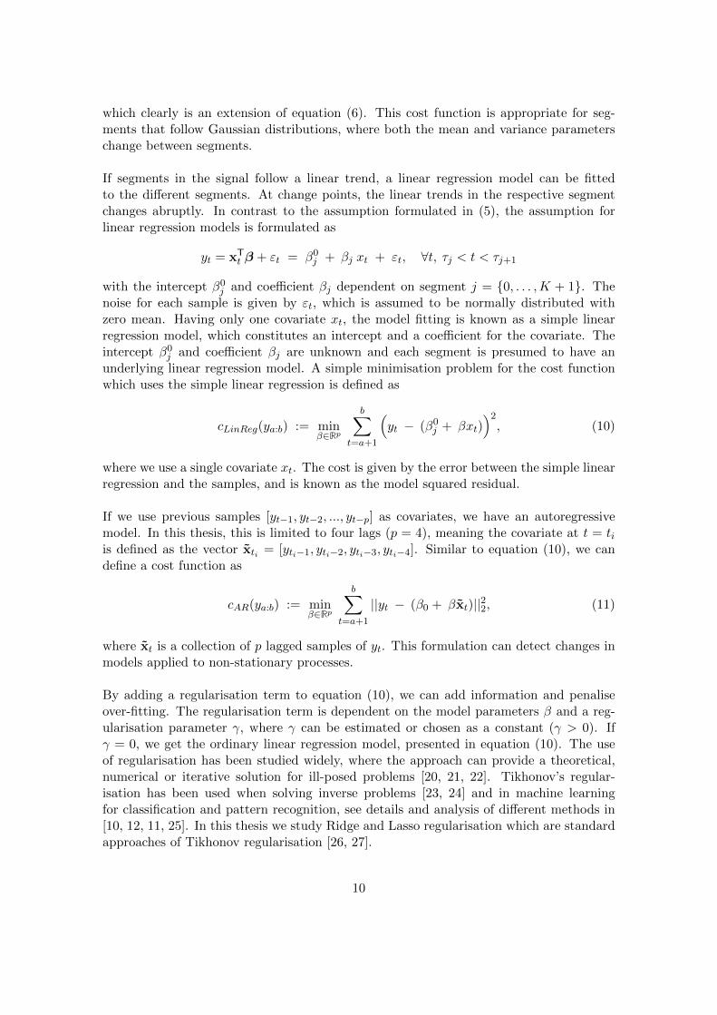
which clearly is an extension of equation (6). This cost function is appropriate for seg-ments that follow Gaussian distributions, where both the mean and variance parameterschange between segments.

If segments in the signal follow a linear trend, a linear regression model can be fittedto the different segments. At change points, the linear trends in the respective segmentchanges abruptly. In contrast to the assumption formulated in (5), the assumption forlinear regression models is formulated as

yt = xTt β + εt = β0

j + βj xt + εt, ∀t, τj < t < τj+1

with the intercept β0j and coefficient βj dependent on segment j = {0, . . . ,K + 1}. The

noise for each sample is given by εt, which is assumed to be normally distributed withzero mean. Having only one covariate xt, the model fitting is known as a simple linearregression model, which constitutes an intercept and a coefficient for the covariate. Theintercept β0

j and coefficient βj are unknown and each segment is presumed to have anunderlying linear regression model. A simple minimisation problem for the cost functionwhich uses the simple linear regression is defined as

cLinReg(ya:b) := minβ∈Rp

b∑t=a+1

(yt − (β0

j + βxt))2, (10)

where we use a single covariate xt. The cost is given by the error between the simple linearregression and the samples, and is known as the model squared residual.

If we use previous samples [yt−1, yt−2, ..., yt−p] as covariates, we have an autoregressivemodel. In this thesis, this is limited to four lags (p = 4), meaning the covariate at t = tiis defined as the vector xti = [yti−1, yti−2, yti−3, yti−4]. Similar to equation (10), we candefine a cost function as

cAR(ya:b) := minβ∈Rp

b∑t=a+1

||yt − (β0 + βxt)||22, (11)

where xt is a collection of p lagged samples of yt. This formulation can detect changes inmodels applied to non-stationary processes.

By adding a regularisation term to equation (10), we can add information and penaliseover-fitting. The regularisation term is dependent on the model parameters β and a reg-ularisation parameter γ, where γ can be estimated or chosen as a constant (γ > 0). Ifγ = 0, we get the ordinary linear regression model, presented in equation (10). The useof regularisation has been studied widely, where the approach can provide a theoretical,numerical or iterative solution for ill-posed problems [20, 21, 22]. Tikhonov’s regular-isation has been used when solving inverse problems [23, 24] and in machine learningfor classification and pattern recognition, see details and analysis of different methods in[10, 12, 11, 25]. In this thesis we study Ridge and Lasso regularisation which are standardapproaches of Tikhonov regularisation [26, 27].

10

The first regularisation approach which is studied in this thesis is the Ridge regression,

cRidge(ya:b) := minβ∈Rp

b∑t=a+1

(yt − (β0 + βxt)

)2+ γ

p∑j=1

||βj ||22, (12)

where the regularisation term is the aggregated squared L2-norm of the model coeffi-cients. If the L2-norm is exchanged for the L1-norm we get Lasso regularisation. The costfunctions is defined as

cLasso(ya:b) := minβ∈Rp

b∑t=a+1

(yt − (β0 + βxt)

)2+ γ

p∑j=1

|βj | (13)

where γ is the previously described regularisation parameter. Note that this parametercan be the same as the parameter in the Ridge regression (12) but these are not necessarilyequal.

2.3 Bayesian approach

In contrast to the optimisation approach, the Bayesian approach is based on Bayes’ proba-bility theorem, where the maximum probabilities are identified. It is based on the Bayesianprinciple of calculating a posterior distribution of a time stamp being a change point, givena prior and a likelihood function. From this posterior distribution, we can identify thepoints which are most likely to be change points. The upcoming section will briefly gothrough the theory behind the Bayesian approach. For more details and proofs of usedTheorem, the reader is directed to the work by Fearnhead [9]. The section is formulatedas a derivation of the sought after posterior distribution for the change points. Usingtwo probabilistic quantities P and Q, we can rewrite Bayes’ formula to a problem specificformulation which gives the posterior probability of a change point τ . Finally, we com-bine the individual posterior distribution to get a joint distribution for all possible changepoints.

The principle behind the Bayesian approach lies in the probabilistic relationship formu-lated by Bayes in 1976 [28], where a posterior probability distribution can be expressedas

Pr(a|b) =Pr(a, b)

Pr(b)=

Pr(b|a) Pr(a)

Pr(b)(14)

for the event a given another event b. Here, Pr(b|a) is the likelihood of b given a. Thedistribution Pr(a) is known as the prior distribution of a. As soon as Pr(b|a) and Pr(a)are defined, the estimator of the posterior distribution Pr(a|b) can be calculated. Acommon technique is the Maximum A Posteriori (MAP) approach, which is the solutionof the problem

MAP (b) = maxa∈A

Pr(a|b),

where A are the possible values for a. Taking the log of the above equation, we get

maxa∈A

log Pr(a|b) = maxa∈A

[ log Pr(b|a) + log Pr(a)− log Pr(b) ] (15)

11

which is used in this work.

In our case, we wish to predict the probability of a change point τ given the data. Thus,Bayes’ formula in (14) can be reformulated for our problem as

Pr(τ |y1:n) =Pr(τ, y1:n)

Pr(y1:n)=

Pr(y1:τ |τ) Pr(yτ+1:n|τ) Pr(τ)

Pr(y1:n)(16)

where Pr(y1:τ |τ) and Pr(yτ+1:n|τ) are the likelihood of segments before and after thegiven change point τ . The prior distribution Pr(τ) indicates the probability of a potentialchange point τ existing and y1:n represents the entirety of the signal. Using the MAP(y)in logarithmic terms, we get the problem specific version of (15)

maxτ∈[0:n]

log Pr(τ |y1:n) = maxτ∈[0:n]

[log Pr(y1:τ |τ) + log Pr(yτ+1:n|τ) + log Pr(τ)− log Pr(y1:n)].

Similarly to Fearnhead [9], we will define two functions P and Q which are used forcalculations in the Bayesian approach. First, we define the probability of a segmentP (t, s), given two entries belonging to the same segment

P (t, s) = Pr(yt:s|t, s ∈ Sj) =

∫ s∏i=t

f(yi|θSj ) π(θSj ) dθSj , (17)

where f is the probability density function of entry yt belonging to a segment Sj withparameter θSj . We note that this function has similarities used in the optimisation ap-proach, namely in equation (5), where we assume a distribution for each segment. In thiswork, this likelihood will be the Gaussian observation log-likelihood function, but otherfunction choices can be made. Note that π(θSj ) is the prior for the parameters of segmentSj . The discrete intervals [t, s], t ≤ s makes P an upper triangular matrix which elementsare probabilities for segments yt:s. Note that this probability is independent of the numberof true change points K.

The second function, Q, indicates the probability of a final segment yt:n starting at timeti given a change point at previous time step, ti−1. This probability is affected by thenumber of change points K, and also which of the change points that is located at timeti−1. Since we do not know the exact number of change points K, we use a generic variablek, and perform calculations for all possible values of K. The recurrent function is defined

Q(k)j (i) = Pr(yi:n|τj = i− 1, k) =

=

n−k+j∑s=i

P (t, s) Q(k)j+1(s+ 1) πk(τj = i− 1|τj+1 = s) (18)

Q(k)(1) = Pr(y1:n|k) =

=n−k∑s=1

P (1, s) Q(k)1 (s+ 1) (19)

where Q(k)(1) is the first time step and is a special case of Q(k)j (i). The time index

is indicated with i ∈ [2, . . . , n]. The assumed number of change points is denoted k ∈

12

{1, . . . , n − 1}, where j ∈ {1, . . . , k} indicates which of the k assumed change points weare currently at. The prior πk is based on the distance between change points, naturallydependent on k. This prior can be any point process, where the simplest example isthe constant prior with probability p = 1/n, where n is the number of samples. Otherexamples include the negative binomial and Poisson distribution. Note that the priorshould be a point process since we have discrete time steps. The first time step is definedas an altered function in (19). The result from this recursion is saved in an array of lengthn. A derivation and proof for this function Q is provided by Fearnhead in Theorem 1[9]. When calculating the sums in equations (18)-(19), the terms on the right hand sidecontribute to the function value. We can implement a truncation, with negligible error,at the k-th term if

P (t, k) Q(s+ 1) π(k + 1− t)∑ks=t P (t, s) Q(s+ 1) π(s+ 1− t)

< ε,

where π represents the prior distribution for the distance between two consecutive changepoints and ε is a truncation threshold. This work has used ε = 10−10 as truncation thresh-old.

Using P and Q, the posterior distribution Pr(τj |τj−1, y1:n, k) for change point τj , given theprevious change point τj−1, the data y1:n and number of change points, can be calculated.Substituting in equation (16) along with the expressions for P and Q, in equation (17)and (18) respectively, we can formulate the posterior distribution as

Pr(τj |τj−1, y1:n, k) =

=Pr(yτj−1+1:τj |τj−1 + 1, τj ∈ Sj) Pr(yτj+1:n|τj , k) πk(τj−1|τj)

Pr(yτj−1:n|τj−1, k)=

=P (τj−1 + 1, τj) Q

(k)j (τj + 1) πk(τj−1|τj)

Q(k)j−1(τj−1)

, (20)

where

Pr(τ1|y1:n, k) =P (1, τ1) Q(k)(τ1 + 1) πk(τ1)

Q(k)(1). (21)

Here, πk is the probability of τj based on the distance to τj−1. This posterior distri-bution indicates the probability of change point τj occurring in each possible time stepti ∈ [1, n − 1]. The formulas in (20) and (21) can be applied for each possible number ofchange points, where k can range from 1 to n − 1. Therefore, this posterior distributionis calculated for every available number of change points k.

The final step in the Bayesian approach is to combine the conditional probabilities foreach individual change point (seen in equation (20)) to get the joint distribution for allavailable change points. The joint probability is calculated as

Pr(τ1, τ2, . . . , τn−1|y1:n) =( n−1∏j=2

Pr(τj |τj−1, y1:n, k))

Pr(τ1|y1:n, k), (22)

13

where the first change point τ1 has a different probability formulation due to not havingany previous change point. We can also note that the product is changed to a sumif logarithmic probabilities are used, as in (15). This joint probability can be used toidentify the most likely change points. Examples of calculated posterior distributions arefound in Appendix A, where we see the varying probability of being a change point foreach sample in the dataset. A sampling method can be used to draw samples from thejoint posterior distribution, where we are interested in the points that are most likely tobe change points. This means taht we can identify the peaks in the posterior distribution,above a set confidence level. This is explained further in section 3.3.

Algorithm 3: Pseudo-code for the Bayesian approach

Result: Probability of being a change point, for each time step.Input: Data signal y, prior distribution π, likelihood function, truncation limit.

#Backwards propagation

for t = n− 1 to 1 dofor s = t to n− 1 do

P (s, t) = Pr[ys:t|s, t belong to same segment]endQ(t) = Pr[yt:n|τj = t− 1] =

=∑n−1

s=t Pr[Change points at s ∈ [t, n− 1]]+Pr[No further change points]

end

#Forward propagation

for j = 1 to n− 1 dofor t = j to n− 1 do

PostCP(j, t) = Pr[τj |τj−1, yt:n]end

end

2.4 Methods of error estimation

In this section, the used metrics for evaluating the performance of the CPD algorithms arepresented. We first differentiate between the true change points and the estimated ones.The true change points are denoted by T ∗ = {τ∗0 , . . . , τ∗K+1} while T = {τ0, . . . , τK+1}indicate estimations. Similarly, the number of true change points is indicated K∗ while Krepresents the number of predicted points.

The most straight forward measure is to compare the number of predictions with thetrue number of change points. This is know as the Annotation error, and is defined as

AE := |K −K∗|, (23)

where K is the estimated and K∗ the true change points. This does not indicate howprecise the estimations are, but can indicate if the model is over- or under-fitted.

14

Another similarity metric of interest is the Rand Index (RI) [3]. Compared to the previousdistance metrics, the rand index gives the similarity between two segmentations as apercentage of agreement. This metric is commonly used to compare clustering algorithms.To calculate the index, we need to define two additional sets which indicate whether twosamples are grouped together by a given segmentation or if they are not grouped together.These sets are defined by Truonga et al [3] as

GR(T ) := {(s, t), 1 ≤ s < t ≤ T : s and t belong to the same segment in T },NGR(T ) := {(s, t), 1 ≤ s < t ≤ T : s and t belong to different segments in T },

where T is some segmentation for a time interval [1, T ]. Using these definitions, the randindex is calculated as

RI(T , T ∗) :=|GR(T ) ∩GR(T ∗)|+ |NGR(T ) ∩NGR(T ∗)|

T (T − 1)

which gives the number of agreements divided by possible combinations.

To better understand how well the predictions match the actual change points, one canuse the measure called the meantime error which calculates the meantime between eachprediction to the closest actual change point. The meantime should also be consideredjointly with the dataset because the same magnitude of meantime error can indicate dif-ferent things in different datasets. For real-life time series data, the meantime error shouldbe recorded in units of time, such as seconds, in order to make the results intuitive for theuser to interpret. The meantime is calculated as

MT (T , T ∗) =

∑Kj=1 minτ∗∈T ∗ |τj − τ∗|

K.

A drawback with this measure is that it focuses on the predicted points. If there are fewerpredictions than actual change points, the meantime might be lower if the predictions arein proximity of some of the actual change points but not all. Note that the meantime iscalculated from the prediction and does not necessarily map the prediction to correspond-ing true change point, only the closest one.

Two of the most common metrics of accuracy in predictions are precision and recall.These metrics give a percentage of how well the predictions reflect the true values. Theprecision metric is the fraction of correctly identified predictions over the total number ofpredictions, while the recall metric compares the number of identified true change pointsover the total number of true change points. These metrics can be expressed as

precision =|TP(T , T ∗)||T |

, recall =|TP(T , T ∗)||T ∗|

, (24)

where TP represents the number of true positives between the estimations T and truechange points T ∗. Mathematically, TP is defined as

TP(T , T ∗) = {τ∗ ∈ T ∗|τ ∈ T : |τ∗ − τ | < ε},

15

where ε is some chosen threshold. The threshold gives the radius of acceptance, meaningthe acceptable number of time steps which can differ between prediction and true value.The two metrics (24) can be incorporated into a combined metric, known as the F-score.The metric F1-score uses the harmonic mean of the precision and recall and is appliedin this work. As reviewed in this section, the metrics measure the similarity between thepredicted change points and the actual change points from various perspectives. Hencethis work adopt all of them to give a comprehensive evaluation of the performance of CPDalgorithms.

3 Method

In this section we explore the setting in which the tests are preformed, along with thetesting procedure. First, a description of the simulated datasets are provided, along withmathematical formulas and assumptions. Then, we explore the real world dataset with fourprocess variables. Finally, the testing procedure is described along with adjustments madefor a fair comparison or to reduce computational complexity. All datasets are describedmathematically and illustrated in figures with the true change points indicated as theboarder between two segments. All tests shown in this work can be reproduced using theGIT repositories presented in Appendix B.

3.1 Simulation of data

To investigate the performance of the approaches with certain features present in the data,simulated datasets might be beneficial to use. The complexity of the datasets can varyand this work studies six simulated datasets. The first four datasets investigate the perfor-mance in piecewise constant, piecewise linear, changing variance and autoregressive datarespectively. The fifth and sixth datasets indicate realistic processes, with periodic phe-nomena and non-linear behaviours. Each dataset is explained individually in the followingsections.

Piecewise constant

To generate the simulated data, we have created segments with randomised traits (namelymean and variance) and concatenate to get a segmented dataset. If we randomise a meanand variance, we can create a piecewise constant dataset; an example of such data isshown in Figure 3. In this dataset, we have changes in the mean and variance occurringsimultaneously, meaning the mean and the variance of each segment are different fromthe mean and the variance of other segments. Each value yt in segment Sj follows theGaussian distribution

yt ∼ N (µj , σj), j ∈ {1, ...,K,K + 1},

where µj ∼ U(−10, 10) and σj ∼ U(−1, 1) are randomised constants for each segment.This dataset should be possible to use for computation of CPD in both optimisation andBayesian approaches, as well as for all cost functions in the optimisation approach. Thisdataset may be one of the most manageable datasets.

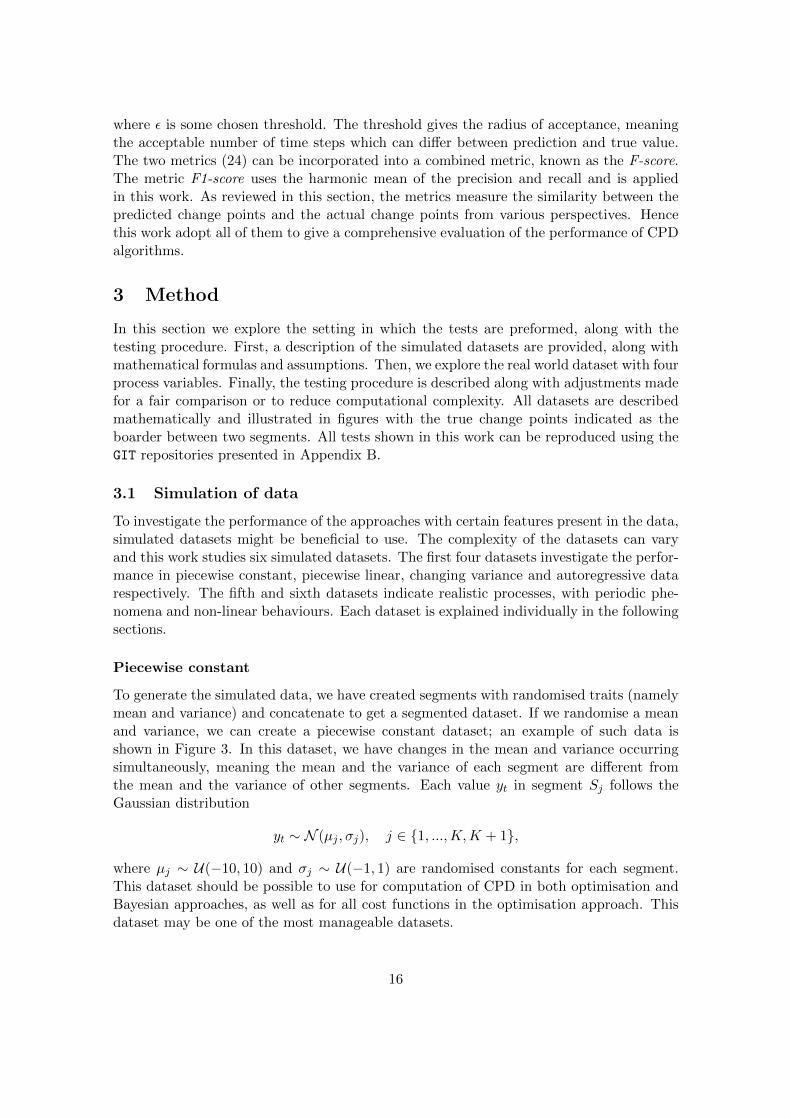
16

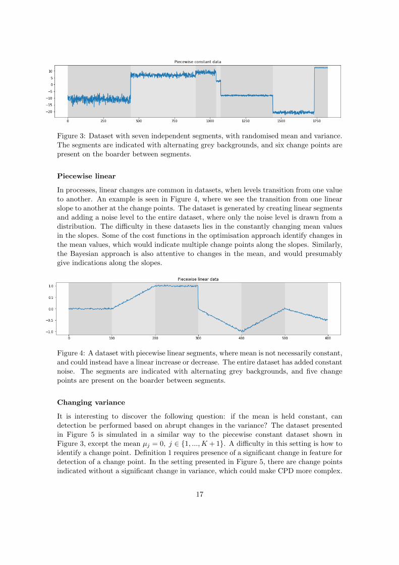
Figure 3: Dataset with seven independent segments, with randomised mean and variance.The segments are indicated with alternating grey backgrounds, and six change points arepresent on the boarder between segments.

Piecewise linear

In processes, linear changes are common in datasets, when levels transition from one valueto another. An example is seen in Figure 4, where we see the transition from one linearslope to another at the change points. The dataset is generated by creating linear segmentsand adding a noise level to the entire dataset, where only the noise level is drawn from adistribution. The difficulty in these datasets lies in the constantly changing mean valuesin the slopes. Some of the cost functions in the optimisation approach identify changes inthe mean values, which would indicate multiple change points along the slopes. Similarly,the Bayesian approach is also attentive to changes in the mean, and would presumablygive indications along the slopes.

Figure 4: A dataset with piecewise linear segments, where mean is not necessarily constant,and could instead have a linear increase or decrease. The entire dataset has added constantnoise. The segments are indicated with alternating grey backgrounds, and five changepoints are present on the boarder between segments.

Changing variance

It is interesting to discover the following question: if the mean is held constant, candetection be performed based on abrupt changes in the variance? The dataset presentedin Figure 5 is simulated in a similar way to the piecewise constant dataset shown inFigure 3, except the mean µj = 0, j ∈ {1, ...,K + 1}. A difficulty in this setting is how toidentify a change point. Definition 1 requires presence of a significant change in feature fordetection of a change point. In the setting presented in Figure 5, there are change pointsindicated without a significant change in variance, which could make CPD more complex.

17

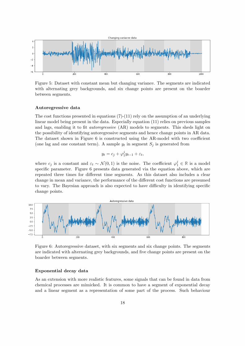
Figure 5: Dataset with constant mean but changing variance. The segments are indicatedwith alternating grey backgrounds, and six change points are present on the boarderbetween segments.

Autoregressive data

The cost functions presented in equations (7)-(11) rely on the assumption of an underlyinglinear model being present in the data. Especially equation (11) relies on previous samplesand lags, enabling it to fit autoregressive (AR) models to segments. This sheds light onthe possibility of identifying autoregressive segments and hence change points in AR data.The dataset shown in Figure 6 is constructed using the AR-model with two coefficient(one lag and one constant term). A sample yt in segment Sj is generated from

yt = cj + ϕj1yt−1 + εt,

where cj is a constant and εt ∼ N (0, 1) is the noise. The coefficient ϕj1 ∈ R is a modelspecific parameter. Figure 6 presents data generated via the equation above, which arerepeated three times for different time segments. As this dataset also includes a clearchange in mean and variance, the performance of the different cost functions are presumedto vary. The Bayesian approach is also expected to have difficulty in identifying specificchange points.

Figure 6: Autoregressive dataset, with six segments and six change points. The segmentsare indicated with alternating grey backgrounds, and five change points are present on theboarder between segments.

Exponential decay data

As an extension with more realistic features, some signals that can be found in data fromchemical processes are mimicked. It is common to have a segment of exponential decayand a linear segment as a representation of some part of the process. Such behaviour

18

can be of practical relevance. For example, the concentration of a chemical in a reactorcan increase linearly when the feed flow of this chemical enters the reactor. Then whenthe reaction starts, the concentration of this chemical decays exponentially. The changepoints between these segments indicate the start and the end of the feed flow injectionphase and the reaction phase. An illustration of such a process is shown in Figure 7 wherethree phases are seen constituting of an exponential decay followed by a linear increase.Similar to the piecewise linear dataset, the signal is created and then noise is added.

Figure 7: Dataset with exponential decay, followed by a linear increase. Segments areindicated with alternating grey backgrounds. In total there are three repeated processes,with six segments and six change points, each at a boarder between indicated segments.

Oscillating dataset

Another common phenomenon in processes is a stabilising process when a level is reached.This can be represented as a damped oscillation

yt = e−dt · cos(t),

where d ≥ 0 is a damping constant. In real world applications it is interesting to detectthe point where the stable level is reached, but does not indicate a significant changein features and is, therefore, not a true change point according to the Definition 1. InFigure 8 illustrates a scaled sigmoid function with added oscillations when the target levelis reached. Such oscillatory and stabilising behaviours can often be seen in controlledvariables in chemical processes. The two features making this dataset more complex arethe sigmoid function and the oscillations occurring before stabilisation.

19

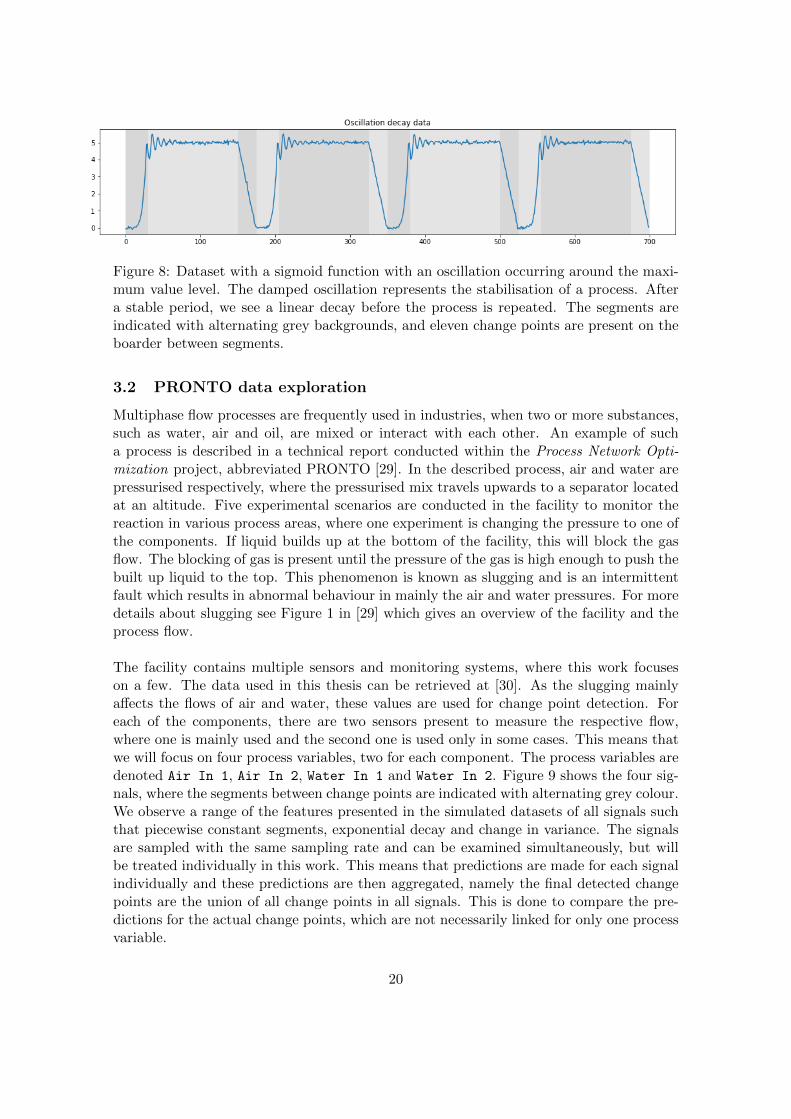
Figure 8: Dataset with a sigmoid function with an oscillation occurring around the maxi-mum value level. The damped oscillation represents the stabilisation of a process. Aftera stable period, we see a linear decay before the process is repeated. The segments areindicated with alternating grey backgrounds, and eleven change points are present on theboarder between segments.

3.2 PRONTO data exploration

Multiphase flow processes are frequently used in industries, when two or more substances,such as water, air and oil, are mixed or interact with each other. An example of sucha process is described in a technical report conducted within the Process Network Opti-mization project, abbreviated PRONTO [29]. In the described process, air and water arepressurised respectively, where the pressurised mix travels upwards to a separator locatedat an altitude. Five experimental scenarios are conducted in the facility to monitor thereaction in various process areas, where one experiment is changing the pressure to one ofthe components. If liquid builds up at the bottom of the facility, this will block the gasflow. The blocking of gas is present until the pressure of the gas is high enough to push thebuilt up liquid to the top. This phenomenon is known as slugging and is an intermittentfault which results in abnormal behaviour in mainly the air and water pressures. For moredetails about slugging see Figure 1 in [29] which gives an overview of the facility and theprocess flow.

The facility contains multiple sensors and monitoring systems, where this work focuseson a few. The data used in this thesis can be retrieved at [30]. As the slugging mainlyaffects the flows of air and water, these values are used for change point detection. Foreach of the components, there are two sensors present to measure the respective flow,where one is mainly used and the second one is used only in some cases. This means thatwe will focus on four process variables, two for each component. The process variables aredenoted Air In 1, Air In 2, Water In 1 and Water In 2. Figure 9 shows the four sig-nals, where the segments between change points are indicated with alternating grey colour.We observe a range of the features presented in the simulated datasets of all signals suchthat piecewise constant segments, exponential decay and change in variance. The signalsare sampled with the same sampling rate and can be examined simultaneously, but willbe treated individually in this work. This means that predictions are made for each signalindividually and these predictions are then aggregated, namely the final detected changepoints are the union of all change points in all signals. This is done to compare the pre-dictions for the actual change points, which are not necessarily linked for only one processvariable.

20

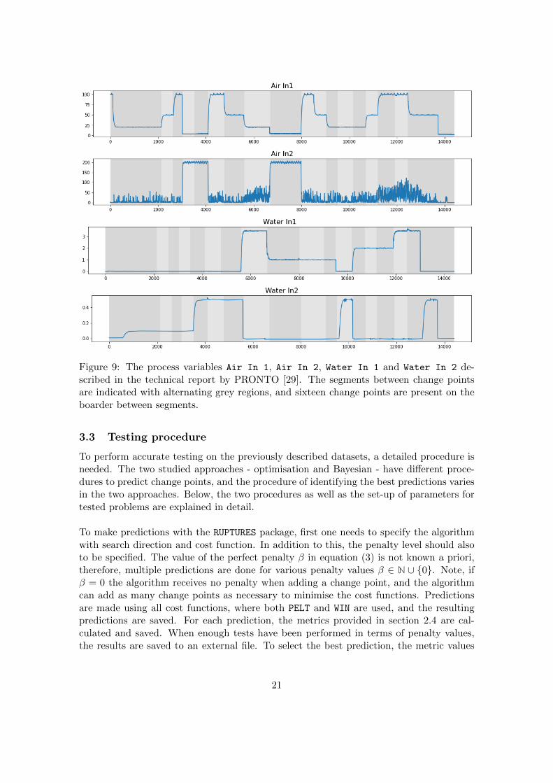
Figure 9: The process variables Air In 1, Air In 2, Water In 1 and Water In 2 de-scribed in the technical report by PRONTO [29]. The segments between change pointsare indicated with alternating grey regions, and sixteen change points are present on theboarder between segments.

3.3 Testing procedure

To perform accurate testing on the previously described datasets, a detailed procedure isneeded. The two studied approaches - optimisation and Bayesian - have different proce-dures to predict change points, and the procedure of identifying the best predictions variesin the two approaches. Below, the two procedures as well as the set-up of parameters fortested problems are explained in detail.

To make predictions with the RUPTURES package, first one needs to specify the algorithmwith search direction and cost function. In addition to this, the penalty level should alsoto be specified. The value of the perfect penalty β in equation (3) is not known a priori,therefore, multiple predictions are done for various penalty values β ∈ N ∪ {0}. Note, ifβ = 0 the algorithm receives no penalty when adding a change point, and the algorithmcan add as many change points as necessary to minimise the cost functions. Predictionsare made using all cost functions, where both PELT and WIN are used, and the resultingpredictions are saved. For each prediction, the metrics provided in section 2.4 are cal-culated and saved. When enough tests have been performed in terms of penalty values,the results are saved to an external file. To select the best prediction, the metric values

21

need to be taken into account. Our goal is to minimise the annotation error and meantimewhilst maximising the F1-score and rand index. Discussion on how to evaluate the metricsand choose the best one for different data is provided in section 5. Obtained results arepresented in section 4 along with respective metric values.

To apply the Bayesian approach for predictions, the computational procedure is differ-ent. Using the concepts derived in section 2.3 we can calculate posterior distribution withprobabilities for each time step being a change point. Due to the algorithm being com-putationally heavy, the resolution of the data is reduced in the real dataset by PRONTOusing Piecewise Aggregate Approximation (PAA) [31]. The function aggregates the valuesof a window to an average value. The used window size is 20 samples. Generally, todraw conclusions from a posterior distribution, sampling is used to create a collection ofpoints which in this case represents the change points. The calculated distribution doesnot follow a simple distribution, which makes sampling complicated. In essence, we wantto create a sample of the most probable change points, without unnecessary duplicates.To draw this type of sample2 of change points from the posterior distribution, the functionfind peaks in the Python package SciPy[32] is used. The function identifies the peaksin a dataset using two parameters: threshold which the peak value should exceed, anddistance which indicates the minimum distance between peaks. The threshold is set to0.2, where we require a certainty level of at least 20%. The distance is set to 10 timesteps to prevent duplicate values. The posterior distribution is calculated once for onedataset, where numerous samples can be drawn using different settings in the find peaks

function. This approach returns the most probable change points which are then used tocalculate the metrics presented in section 2.4.

All signals are handled individually meaning we are only investigating the uni-variatecase, without correlation between the covariates. In the simulated datasets, this is trivialsince we only have one signal per case. In the PRONTO dataset we have four processvariables, which are explained in the previous section. The same prediction algorithm isapplied to all signals, and are not altered between the different process variables. Thismeans that the range of the signals can affect the predictions. To counteract unfair pre-dictions, the process variables are normalised. Normalisation is not necessary for thesignals in the simulated datasets, while the process variables in the PRONTO dataset arenormalised to account for the difference in range in the signals.

4 Results

Given the different search directions and cost functions, presented in sections 2.2.1 and2.2.2 respectively, we can presume that different setups will identify different features andhence differ in the prediction of change points. We can also assume that the Bayesianapproach, presented in section 2.3, will not necessarily give the same predictions as theoptimisation approach. We note that all algorithms predict the intermediate change pointsT = {τ1, ..., τK} along with one artificial change point τK+1 := n. This artificial change

2This is not necessarily a proper sampling methodology, and other approaches can be used instead. Analternative sampling method is provided in Fearnhead [9] (page 8).

22

point is based on definition and is used when the predictions are compared. A first stepto understanding the performance of the different approaches is to simulate datasets withcertain features and compare the obtained metrics. In addition, a visualisation is shownfor each case, with the predicted change point in comparison to the actual change points.In this section, we present the results of the two approaches on the six simulated datasetswith varying complexity, described in section 3.1. Later, the results for the real-worlddata are presented.

4.1 Simulated datasets

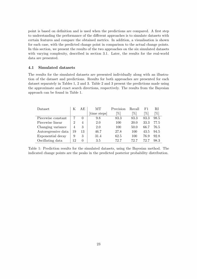
The results for the simulated datasets are presented individually along with an illustra-tion of the dataset and predictions. Results for both approaches are presented for eachdataset separately in Tables 1, 2 and 3. Table 2 and 3 present the predictions made usingthe approximate and exact search directions, respectively. The results from the Bayesianapproach can be found in Table 1.

Dataset K AE MT Precision Recall F1 RI[time steps] [%] [%] [%] [%]

Piecewise constant 7 0 9.8 83.3 83.3 83.3 98.5Piecewise linear 2 4 2.0 100 20.0 33.3 77.5Changing variance 4 3 2.0 100 50.0 66.7 76.5Autoregressive data 19 13 46.7 27.8 100 43.5 94.5Exponential decay 9 3 31.4 62.5 100 76.9 92.8Oscillating data 12 0 3.5 72.7 72.7 72.7 98.3

Table 1: Prediction results for the simulated datasets, using the Bayesian method. Theindicated change points are the peaks in the predicted posterior probability distribution.

23

Dataset Cost Pen K AE MT Precision Recall F1 RIfunction [time steps] [%] [%] [%] [%]

Piecewise constant

cL2 5 6 1 1.2 100 83.3 90.9 99.5cL1 1 7 0 20.8 83.3 83.3 83.3 97.2cNormal 5 6 1 1.4 100 83.3 90.9 99.5cLinReg 424 6 1 57.4 80.0 66.7 72.7 92.4cAR 5 5 2 1.5 100 66.7 80.0 94.7cridge 24 6 1 11.4 100 83.3 90.9 98.1classo 24 6 1 11.4 100 83.3 90.9 98.1

Piecewise linear

cL2 0 5 1 36.3 25.0 20.0 22.2 88.4cL1 0 5 1 33.8 25.0 20.0 22.2 88.7cNormal 0 5 1 7.5 100 80.0 88.9 92.8cLinReg 0 5 1 35.9 25.0 20.0 22.2 88.2cAR 0 6 0 5.0 100 100 100 97.6cridge 0 6 0 0.0 100 100 100 100classo 0 6 0 1.0 100 100 100 100

Changing variance

cL2 0 7 0 42.2 50.0 50.0 50.0 91.3cL1 0 7 0 45.2 66.7 66.7 66.7 90.4cNormal 0 7 0 22.0 83.3 83.3 83.3 92.0cLinReg 0 7 0 42.2 50.0 50.0 50.0 91.3cAR 0 6 1 44.8 60.0 50.0 55.0 87.4cridge 0 3 4 40.5 50.0 16.7 25.0 74.9classo 0 3 4 40.5 50.0 16.7 25.0 74.9

Autoregressive data

cL2 0 7 1 37.5 83.3 100 90.9 91.3cL1 0 7 1 40.0 83.3 100 90.9 90.5cNormal 0 7 1 40.0 83.3 100 90.9 90.5cLinReg 0 7 1 37.5 83.3 100 90.9 91.3cAR 0 6 0 2.0 100 100 100 99.3cridge 0 4 2 71.7 0.0 0.0 0.0 79.4classo 0 4 2 71.7 0.0 0.0 0.0 79.4

Exponential decay

cL2 0 4 2 21.7 66.7 40.0 50.0 89.7cL1 0 5 1 27.5 50.0 40.0 44.4 89.9cNormal 0 6 0 16.0 100 100 100 95.1cLinReg 0 6 0 30.0 60.0 60.0 60.0 92.5cAR 0 7 1 18.3 83.3 100 90.9 98.5cridge 0 6 0 6.0 100 100 100 97.9classo 0 6 0 36.0 80.0 80.0 80.0 89.8

Oscillating data

cL2 0 5 7 7.5 100 36.4 53.3 87.3cL1 0 5 7 8.8 100 36.4 53.3 88.3cNormal 0 8 4 12.9 100 63.6 77.8 93.0cLinReg 0 4 8 0.0 100 27.3 42.9 86.3cAR 0 5 7 10.0 100 36.4 53.3 88.9cridge 0 5 7 8.8 100 36.4 53.3 88.9classo 0 5 7 8.8 100 36.4 53.3 88.9

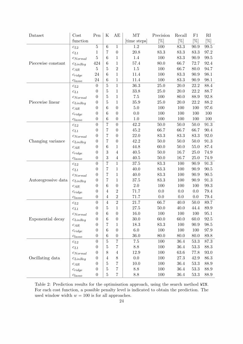
Table 2: Prediction results for the optimisation approach, using the search method WIN.For each cost function, a possible penalty level is indicated to obtain the prediction. Theused window width w = 100 is for all approaches.

24

Dataset Cost Pen K AE MT Precision Recall F1 RIfunction [time steps] [%] [%] [%] [%]

Piecewise constant

cL2 450 7 0 1.7 66.7 66.7 66.7 95.8cL1 15 7 0 1.3 83.3 83.3 83.3 99.8cNormal 10 6 1 3.4 100 83.3 90.9 95.0cLinReg 1000 7 0 99.2 66.7 66.7 66.7 92.6cAR 80 7 0 1.8 66.7 66.7 66.7 94.8cRidge 5 7 0 18.8 83.3 83.3 83.3 98.3cLasso 70 7 0 1.3 83.3 83.3 83.3 99.8

Piecewise linear

cL2 2 6 0 31.0 40.0 40.0 40.0 89.4cL1 6 6 0 30.0 60.0 60.0 60.0 89.8cNormal 120 6 0 23.0 60.0 60.0 60.0 91.8cLinReg 0 5 1 10.0 75.0 60.0 66.7 93.1cAR 0 6 0 4.0 80.0 80.0 80.0 93.1cRidge 0 6 0 0.0 100 100 100 100cLasso 2 6 0 1.0 100 100 100 99.5

Changing variance

cL2 6 8 1 46.4 28.6 33.3 30.8 63.5cL1 3 7 0 47.3 16.7 16.7 16.7 58.8cNormal 9 6 1 3.4 100 83.3 90.9 95.0cLinReg 0 8 1 40.7 57.1 66.7 61.5 91.3cAR 30 6 1 51.2 20.0 16.7 18.2 59.3cRidge 0 9 2 41.0 62.5 83.3 71.4 90.7cLasso 2 8 1 45.6 28.6 33.3 30.8 69.5

Autoregressive data

cL2 320 6 0 40.0 40.0 40.0 40.0 83.4cL1 60 6 0 40.0 40.0 40.0 40.0 83.4cNormal 100 6 0 40.0 40.0 40.0 40.0 83.4cLinReg 145 6 0 28.0 80.0 80.0 80.0 93.4cAR 30 6 0 2.0 100 100 100 99.3cRidge 10 6 0 50.0 40.0 40.0 40.0 86.0cLasso 50 6 0 39.0 40.0 40.0 40.0 82.9

Exponential decay

cL2 20 6 0 26.0 100 100 100 93.5cL1 20 6 0 25.0 100 100 100 93.6cNormal 200 7 1 40.0 83.3 100 90.9 91.8cLinReg 5 6 0 12.0 100 100 100 96.7cAR 0 8 2 1.4 71.4 100 83.3 99.5cRidge 15 6 0 3.0 100 100 100 99.1cLasso 35 6 0 4.0 100 100 100 98.8

Oscillating data

cL2 15 12 0 6.8 72.7 72.7 72.7 97.0cL1 10 12 0 5.9 72.7 72.7 72.7 97.1cNormal 75 12 0 8.2 81.8 81.8 81.8 95.6cLinReg 0 5 7 12.5 75.0 27.3 40.0 87.5cAR 1 12 0 5.0 72.7 72.7 72.7 96.8cRidge 0 6 6 24.0 60.0 27.3 37.5 89.7cLasso 10 12 0 1.8 72.7 72.7 72.7 98.9

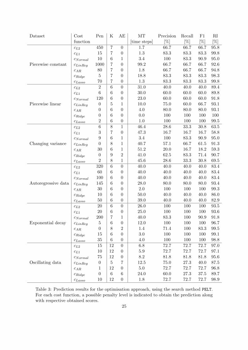
Table 3: Prediction results for the optimisation approach, using the search method PELT.For each cost function, a possible penalty level is indicated to obtain the prediction alongwith respective obtained scores.

25

4.1.1 Piecewise constant data

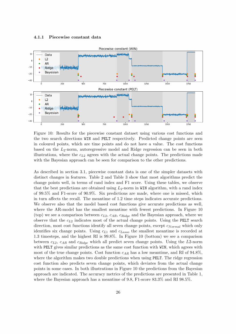
Figure 10: Results for the piecewise constant dataset using various cost functions andthe two search directions WIN and PELT respectively. Predicted change points are seenin coloured points, which are time points and do not have a value. The cost functionsbased on the L2-norm, autoregressive model and Ridge regression can be seen in bothillustrations, where the cL2 agrees with the actual change points. The predictions madewith the Bayesian approach can be seen for comparison to the other predictions.

As described in section 3.1, piecewise constant data is one of the simpler datasets withdistinct changes in features. Table 2 and Table 3 show that most algorithms predict thechange points well, in terms of rand index and F1 score. Using these tables, we observethat the best predictions are obtained using L2-norm in WIN algorithm, with a rand indexof 99.5% and F1-score of 90.9%. Six predictions are made, where one is missed, whichin turn affects the recall. The meantime of 1.2 time steps indicates accurate predictions.We observe also that the model based cost functions give accurate predictions as well,where the AR-model has the smallest meantime with fewest predictions. In Figure 10(top) we see a comparison between cL2, cAR, cRidge and the Bayesian approach, where weobserve that the cL2 indicates most of the actual change points. Using the PELT searchdirection, most cost functions identify all seven change points, except cNormal which onlyidentifies six change points. Using cL1 and cLasso the smallest meantime is recorded at1.3 timesteps, and the highest RI is 99.8%. In Figure 10 (bottom) we see a comparisonbetween cL2, cAR and cRidge which all predict seven change points. Using the L2-normwith PELT gives similar predictions as the same cost function with WIN, which agrees withmost of the true change points. Cost function cAR has a low meantime, and RI of 94.8%,where the algorithm makes two double predictions when using PELT. The ridge regressioncost function also predicts seven change points, which deviates from the actual changepoints in some cases. In both illustrations in Figure 10 the predictions from the Bayesianapproach are indicated. The accuracy metrics of the predictions are presented in Table 1,where the Bayesian approach has a meantime of 9.8, F1-score 83.3% and RI 98.5%.

26

4.1.2 Piecewise linear data

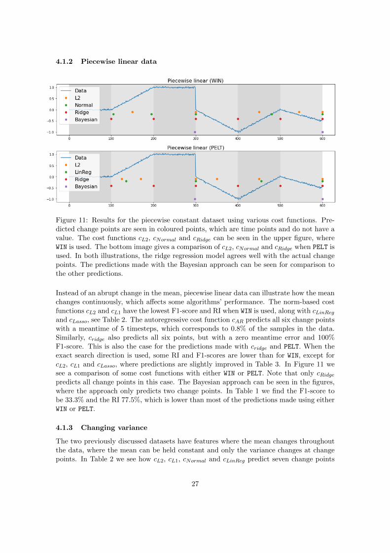
Figure 11: Results for the piecewise constant dataset using various cost functions. Pre-dicted change points are seen in coloured points, which are time points and do not have avalue. The cost functions cL2, cNormal and cRidge can be seen in the upper figure, whereWIN is used. The bottom image gives a comparison of cL2, cNormal and cRidge when PELT isused. In both illustrations, the ridge regression model agrees well with the actual changepoints. The predictions made with the Bayesian approach can be seen for comparison tothe other predictions.

Instead of an abrupt change in the mean, piecewise linear data can illustrate how the meanchanges continuously, which affects some algorithms’ performance. The norm-based costfunctions cL2 and cL1 have the lowest F1-score and RI when WIN is used, along with cLinRegand cLasso, see Table 2. The autoregressive cost function cAR predicts all six change pointswith a meantime of 5 timesteps, which corresponds to 0.8% of the samples in the data.Similarly, cridge also predicts all six points, but with a zero meantime error and 100%F1-score. This is also the case for the predictions made with cridge and PELT. When theexact search direction is used, some RI and F1-scores are lower than for WIN, except forcL2, cL1 and cLasso, where predictions are slightly improved in Table 3. In Figure 11 wesee a comparison of some cost functions with either WIN or PELT. Note that only cRidgepredicts all change points in this case. The Bayesian approach can be seen in the figures,where the approach only predicts two change points. In Table 1 we find the F1-score tobe 33.3% and the RI 77.5%, which is lower than most of the predictions made using eitherWIN or PELT.

4.1.3 Changing variance

The two previously discussed datasets have features where the mean changes throughoutthe data, where the mean can be held constant and only the variance changes at changepoints. In Table 2 we see how cL2, cL1, cNormal and cLinReg predict seven change points

27

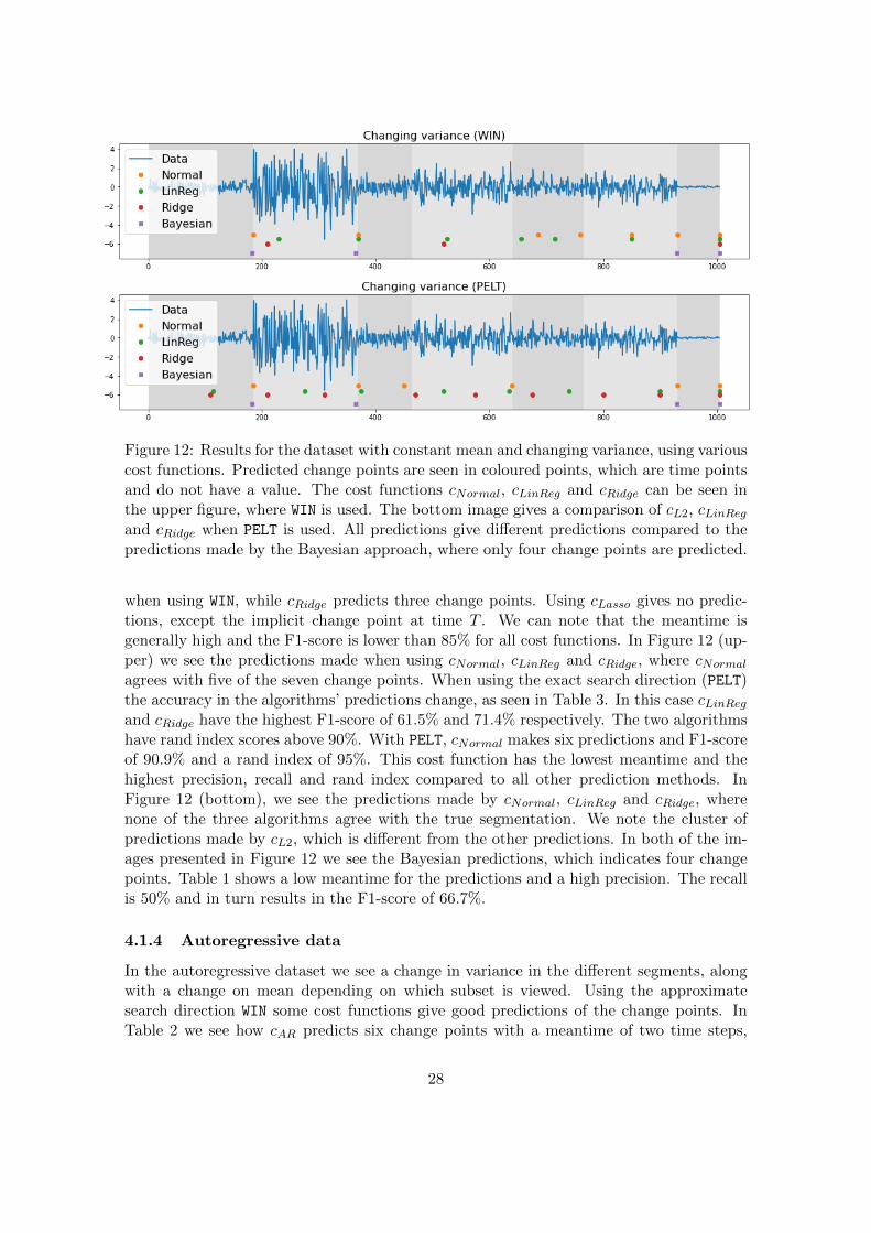
Figure 12: Results for the dataset with constant mean and changing variance, using variouscost functions. Predicted change points are seen in coloured points, which are time pointsand do not have a value. The cost functions cNormal, cLinReg and cRidge can be seen inthe upper figure, where WIN is used. The bottom image gives a comparison of cL2, cLinRegand cRidge when PELT is used. All predictions give different predictions compared to thepredictions made by the Bayesian approach, where only four change points are predicted.

when using WIN, while cRidge predicts three change points. Using cLasso gives no predic-tions, except the implicit change point at time T . We can note that the meantime isgenerally high and the F1-score is lower than 85% for all cost functions. In Figure 12 (up-per) we see the predictions made when using cNormal, cLinReg and cRidge, where cNormalagrees with five of the seven change points. When using the exact search direction (PELT)the accuracy in the algorithms’ predictions change, as seen in Table 3. In this case cLinRegand cRidge have the highest F1-score of 61.5% and 71.4% respectively. The two algorithmshave rand index scores above 90%. With PELT, cNormal makes six predictions and F1-scoreof 90.9% and a rand index of 95%. This cost function has the lowest meantime and thehighest precision, recall and rand index compared to all other prediction methods. InFigure 12 (bottom), we see the predictions made by cNormal, cLinReg and cRidge, wherenone of the three algorithms agree with the true segmentation. We note the cluster ofpredictions made by cL2, which is different from the other predictions. In both of the im-ages presented in Figure 12 we see the Bayesian predictions, which indicates four changepoints. Table 1 shows a low meantime for the predictions and a high precision. The recallis 50% and in turn results in the F1-score of 66.7%.

4.1.4 Autoregressive data

In the autoregressive dataset we see a change in variance in the different segments, alongwith a change on mean depending on which subset is viewed. Using the approximatesearch direction WIN some cost functions give good predictions of the change points. InTable 2 we see how cAR predicts six change points with a meantime of two time steps,

28

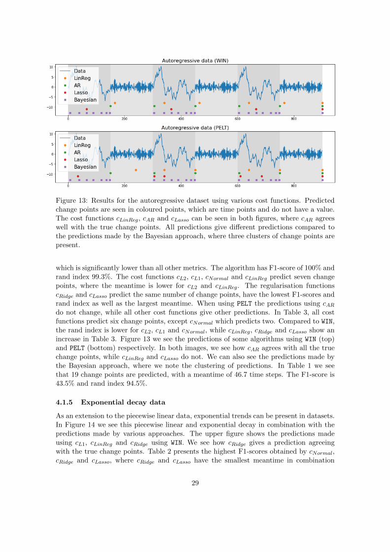
Figure 13: Results for the autoregressive dataset using various cost functions. Predictedchange points are seen in coloured points, which are time points and do not have a value.The cost functions cLinReg, cAR and cLasso can be seen in both figures, where cAR agreeswell with the true change points. All predictions give different predictions compared tothe predictions made by the Bayesian approach, where three clusters of change points arepresent.

which is significantly lower than all other metrics. The algorithm has F1-score of 100% andrand index 99.3%. The cost functions cL2, cL1, cNormal and cLinReg predict seven changepoints, where the meantime is lower for cL2 and cLinReg. The regularisation functionscRidge and cLasso predict the same number of change points, have the lowest F1-scores andrand index as well as the largest meantime. When using PELT the predictions using cARdo not change, while all other cost functions give other predictions. In Table 3, all costfunctions predict six change points, except cNormal which predicts two. Compared to WIN,the rand index is lower for cL2, cL1 and cNormal, while cLinReg, cRidge and cLasso show anincrease in Table 3. Figure 13 we see the predictions of some algorithms using WIN (top)and PELT (bottom) respectively. In both images, we see how cAR agrees with all the truechange points, while cLinReg and cLasso do not. We can also see the predictions made bythe Bayesian approach, where we note the clustering of predictions. In Table 1 we seethat 19 change points are predicted, with a meantime of 46.7 time steps. The F1-score is43.5% and rand index 94.5%.

4.1.5 Exponential decay data

As an extension to the piecewise linear data, exponential trends can be present in datasets.In Figure 14 we see this piecewise linear and exponential decay in combination with thepredictions made by various approaches. The upper figure shows the predictions madeusing cL1, cLinReg and cRidge using WIN. We see how cRidge gives a prediction agreeingwith the true change points. Table 2 presents the highest F1-scores obtained by cNormal,cRidge and cLasso, where cRidge and cLasso have the smallest meantime in combination

29

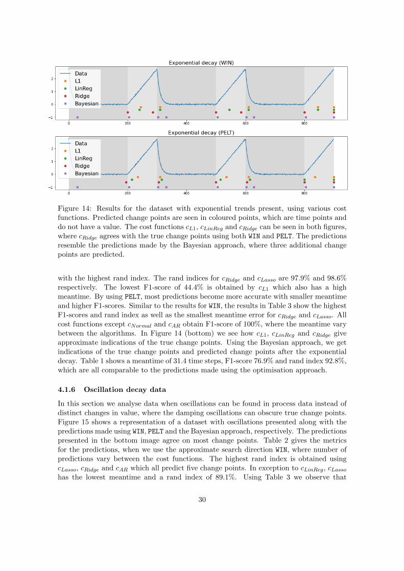
Figure 14: Results for the dataset with exponential trends present, using various costfunctions. Predicted change points are seen in coloured points, which are time points anddo not have a value. The cost functions cL1, cLinReg and cRidge can be seen in both figures,where cRidge agrees with the true change points using both WIN and PELT. The predictionsresemble the predictions made by the Bayesian approach, where three additional changepoints are predicted.

with the highest rand index. The rand indices for cRidge and cLasso are 97.9% and 98.6%respectively. The lowest F1-score of 44.4% is obtained by cL1 which also has a highmeantime. By using PELT, most predictions become more accurate with smaller meantimeand higher F1-scores. Similar to the results for WIN, the results in Table 3 show the highestF1-scores and rand index as well as the smallest meantime error for cRidge and cLasso. Allcost functions except cNormal and cAR obtain F1-score of 100%, where the meantime varybetween the algorithms. In Figure 14 (bottom) we see how cL1, cLinReg and cRidge giveapproximate indications of the true change points. Using the Bayesian approach, we getindications of the true change points and predicted change points after the exponentialdecay. Table 1 shows a meantime of 31.4 time steps, F1-score 76.9% and rand index 92.8%,which are all comparable to the predictions made using the optimisation approach.

4.1.6 Oscillation decay data

In this section we analyse data when oscillations can be found in process data instead ofdistinct changes in value, where the damping oscillations can obscure true change points.Figure 15 shows a representation of a dataset with oscillations presented along with thepredictions made using WIN, PELT and the Bayesian approach, respectively. The predictionspresented in the bottom image agree on most change points. Table 2 gives the metricsfor the predictions, when we use the approximate search direction WIN, where number ofpredictions vary between the cost functions. The highest rand index is obtained usingcLasso, cRidge and cAR which all predict five change points. In exception to cLinReg, cLassohas the lowest meantime and a rand index of 89.1%. Using Table 3 we observe that

30

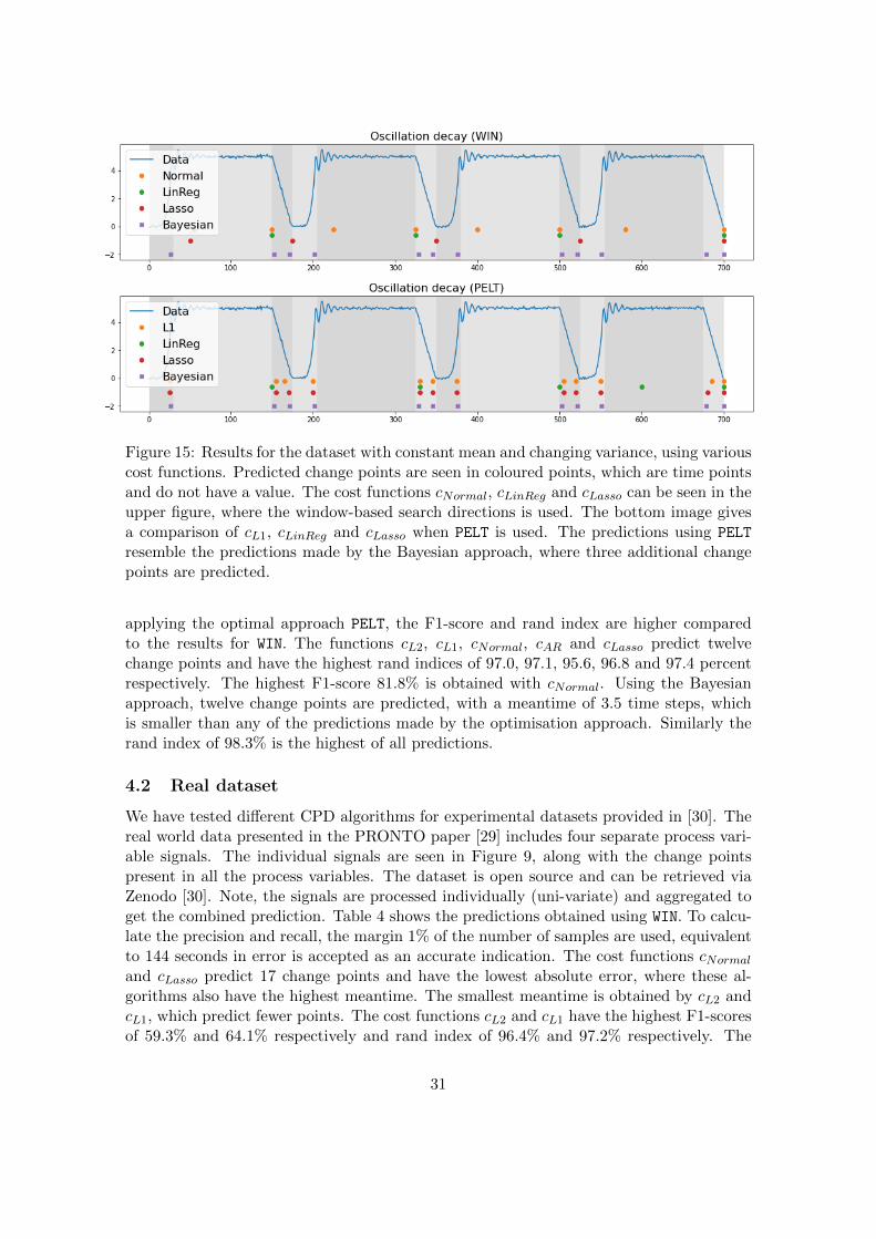
Figure 15: Results for the dataset with constant mean and changing variance, using variouscost functions. Predicted change points are seen in coloured points, which are time pointsand do not have a value. The cost functions cNormal, cLinReg and cLasso can be seen in theupper figure, where the window-based search directions is used. The bottom image givesa comparison of cL1, cLinReg and cLasso when PELT is used. The predictions using PELT

resemble the predictions made by the Bayesian approach, where three additional changepoints are predicted.

applying the optimal approach PELT, the F1-score and rand index are higher comparedto the results for WIN. The functions cL2, cL1, cNormal, cAR and cLasso predict twelvechange points and have the highest rand indices of 97.0, 97.1, 95.6, 96.8 and 97.4 percentrespectively. The highest F1-score 81.8% is obtained with cNormal. Using the Bayesianapproach, twelve change points are predicted, with a meantime of 3.5 time steps, whichis smaller than any of the predictions made by the optimisation approach. Similarly therand index of 98.3% is the highest of all predictions.

4.2 Real dataset

We have tested different CPD algorithms for experimental datasets provided in [30]. Thereal world data presented in the PRONTO paper [29] includes four separate process vari-able signals. The individual signals are seen in Figure 9, along with the change pointspresent in all the process variables. The dataset is open source and can be retrieved viaZenodo [30]. Note, the signals are processed individually (uni-variate) and aggregated toget the combined prediction. Table 4 shows the predictions obtained using WIN. To calcu-late the precision and recall, the margin 1% of the number of samples are used, equivalentto 144 seconds in error is accepted as an accurate indication. The cost functions cNormaland cLasso predict 17 change points and have the lowest absolute error, where these al-gorithms also have the highest meantime. The smallest meantime is obtained by cL2 andcL1, which predict fewer points. The cost functions cL2 and cL1 have the highest F1-scoresof 59.3% and 64.1% respectively and rand index of 96.4% and 97.2% respectively. The

31

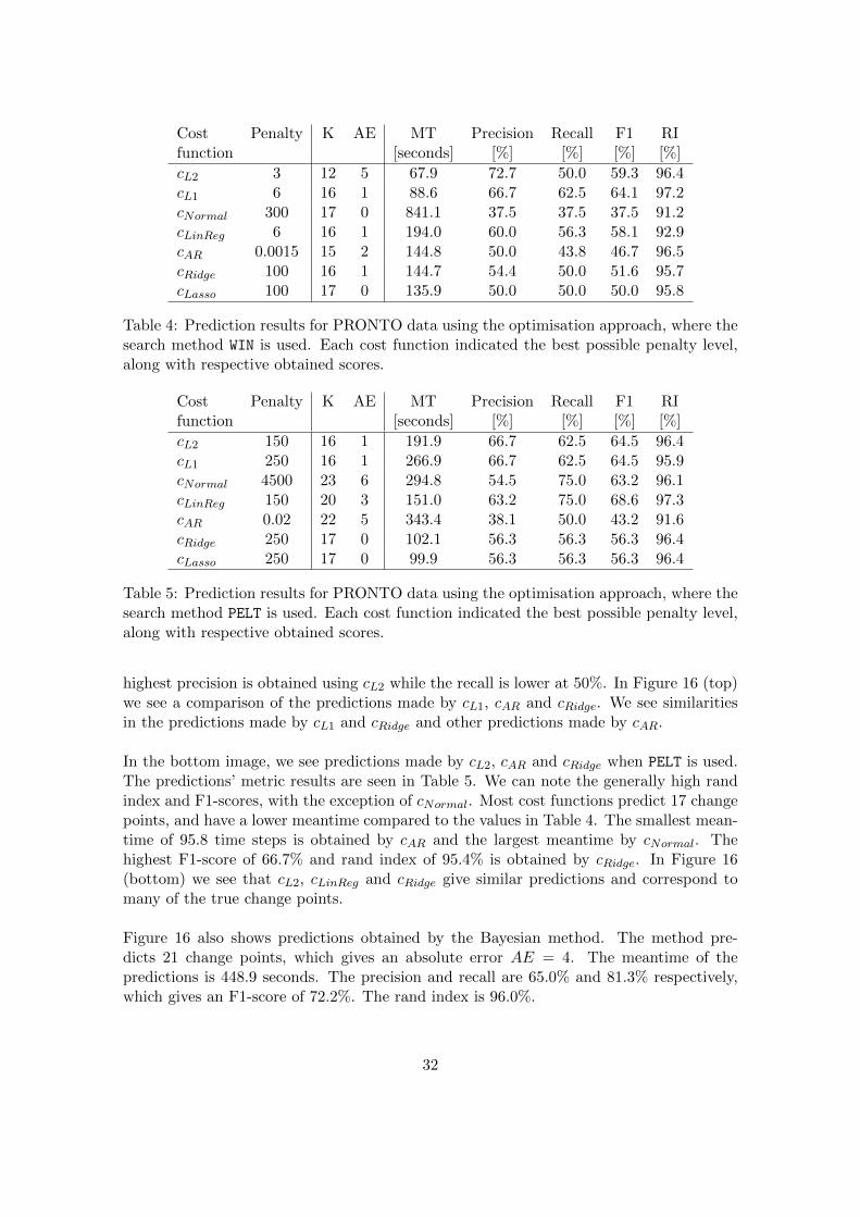
Cost Penalty K AE MT Precision Recall F1 RIfunction [seconds] [%] [%] [%] [%]

cL2 3 12 5 67.9 72.7 50.0 59.3 96.4cL1 6 16 1 88.6 66.7 62.5 64.1 97.2cNormal 300 17 0 841.1 37.5 37.5 37.5 91.2cLinReg 6 16 1 194.0 60.0 56.3 58.1 92.9cAR 0.0015 15 2 144.8 50.0 43.8 46.7 96.5cRidge 100 16 1 144.7 54.4 50.0 51.6 95.7cLasso 100 17 0 135.9 50.0 50.0 50.0 95.8

Table 4: Prediction results for PRONTO data using the optimisation approach, where thesearch method WIN is used. Each cost function indicated the best possible penalty level,along with respective obtained scores.

Cost Penalty K AE MT Precision Recall F1 RIfunction [seconds] [%] [%] [%] [%]

cL2 150 16 1 191.9 66.7 62.5 64.5 96.4cL1 250 16 1 266.9 66.7 62.5 64.5 95.9cNormal 4500 23 6 294.8 54.5 75.0 63.2 96.1cLinReg 150 20 3 151.0 63.2 75.0 68.6 97.3cAR 0.02 22 5 343.4 38.1 50.0 43.2 91.6cRidge 250 17 0 102.1 56.3 56.3 56.3 96.4cLasso 250 17 0 99.9 56.3 56.3 56.3 96.4

Table 5: Prediction results for PRONTO data using the optimisation approach, where thesearch method PELT is used. Each cost function indicated the best possible penalty level,along with respective obtained scores.

highest precision is obtained using cL2 while the recall is lower at 50%. In Figure 16 (top)we see a comparison of the predictions made by cL1, cAR and cRidge. We see similaritiesin the predictions made by cL1 and cRidge and other predictions made by cAR.

In the bottom image, we see predictions made by cL2, cAR and cRidge when PELT is used.The predictions’ metric results are seen in Table 5. We can note the generally high randindex and F1-scores, with the exception of cNormal. Most cost functions predict 17 changepoints, and have a lower meantime compared to the values in Table 4. The smallest mean-time of 95.8 time steps is obtained by cAR and the largest meantime by cNormal. Thehighest F1-score of 66.7% and rand index of 95.4% is obtained by cRidge. In Figure 16(bottom) we see that cL2, cLinReg and cRidge give similar predictions and correspond tomany of the true change points.

Figure 16 also shows predictions obtained by the Bayesian method. The method pre-dicts 21 change points, which gives an absolute error AE = 4. The meantime of thepredictions is 448.9 seconds. The precision and recall are 65.0% and 81.3% respectively,which gives an F1-score of 72.2%. The rand index is 96.0%.

32

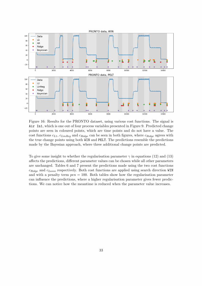
Figure 16: Results for the PRONTO dataset, using various cost functions. The signal isAir In1, which is one out of four process variables presented in Figure 9. Predicted changepoints are seen in coloured points, which are time points and do not have a value. Thecost functions cL1, cLinReg and cRidge can be seen in both figures, where cRidge agrees withthe true change points using both WIN and PELT. The predictions resemble the predictionsmade by the Bayesian approach, where three additional change points are predicted.

To give some insight to whether the regularisation parameter γ in equations (12) and (13)affects the predictions, different parameter values can be chosen while all other parametersare unchanged. Tables 6 and 7 present the predictions made using the two cost functionscRidge and cLasso respectively. Both cost functions are applied using search direction WIN

and with a penalty term pen = 100. Both tables show how the regularisation parametercan influence the predictions, where a higher regularisation parameter gives fewer predic-tions. We can notice how the meantime is reduced when the parameter value increases.

33

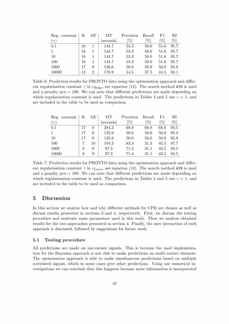
Reg. constant K AE MT Precision Recall F1 RI(γ) [seconds] [%] [%] [%] [%]

0.1 16 1 144.7 53.3 50.0 51.6 95.71 16 1 144.7 53.3 50.0 51.6 95.710 16 1 144.7 53.3 50.0 51.6 95.7100 16 1 144.7 53.3 50.0 51.6 95.71000 17 0 136.6 50.0 50.0 50.0 95.810000 12 2 178.9 54.5 37.5 44.4 93.1

Table 6: Prediction results for PRONTO data using the optimisation approach and differ-ent regularisation constant γ in cRidge, see equation (12). The search method WIN is usedand a penalty pen = 100. We can note that different predictions are made depending onwhich regularisation constant is used. The predictions in Tables 4 and 5 use γ = 1, andare included in the table to be used as comparison.

Reg. constant K AE MT Precision Recall F1 RI(γ) [seconds] [%] [%] [%] [%]

0.1 17 0 284.3 68.8 68.8 68.8 94.51 17 0 135.9 50.0 50.0 50.0 95.810 17 0 135.9 50.0 50.0 50.0 95.8100 7 10 104.3 83.3 31.3 45.5 87.71000 8 9 97.3 71.4 31.1 43.5 94.510000 8 9 97.3 71.4 31.1 43.5 94.5

Table 7: Prediction results for PRONTO data using the optimisation approach and differ-ent regularisation constant γ in cLasso, see equation (13). The search method WIN is usedand a penalty pen = 100. We can note that different predictions are made depending onwhich regularisation constant is used. The predictions in Tables 4 and 5 use γ = 1, andare included in the table to be used as comparison.

5 Discussion

In this section we analyse how and why different methods for CPD are chosen as well asdiscuss results presented in sections 3 and 4, respectively. First, we discuss the testingprocedure and motivate some parameters used in this work. Then we analyse obtainedresults for the two approaches presented in section 4. Finally, the user interaction of eachapproach is discussed, followed by suggestions for future work.

5.1 Testing procedure

All predictions are made on uni-variate signals. This is because the used implementa-tion for the Bayesian approach is not able to make predictions on multi-variate datasets.The optimisation approach is able to make simultaneous predictions based on multiplecorrelated signals, which in some cases give other predictions. Using our numerical in-vestigations we can conclude that this happens because more information is incorporated

34

into the prediction algorithms. Therefore, some change points are detected in the multi-dimensional case and not in the uni-variate case. To make the approaches more compa-rable, predictions are made only using the uni-variate signals and aggregating the resultsfor the signals. This is mainly relevant for the predictions made on the PRONTO dataset,where we have four process variables. The predictions are selected using different methodsfor the two approaches. For the optimisation approach, the penalty term is tuned, whilethe peak thresholds can be tweaked for the Bayesian approach.

Another aspect to discuss is the choice of penalty in the optimisation approach. A benefitwith the approach is that the desired number of change points is not known a priori; wealso do not use the number of predictions as a parameter in the algorithm. The algorithmis applied multiple times with different penalty values, and the best prediction is selectedbased on metric values. This can be computationally heavy if many iterations are neces-sary, but when the appropriate penalty level is found, it can be used for other subsets ofthe same data. We want to minimise AE and meantime, while we want to maximise theF1-score and rand index. Some extra emphasis has also been given to precision over recall,where we value getting an accurate prediction over covering all true change points. Thisis on the basis that some change points might not be identifiable in the dataset but can beof specific interest, according to Definition 2. Using the F1-score as a function of penaltywe will generally find a maximum value. This is since on either side of the maximum,either the recall or precision are lowered due to the number of predictions diverging fromthe true number of change points. The maximum value for the F1-score has generallybeen selected as the best prediction. It should be noted that the results presented in thetables above are not necessarily the only good predictions, and another prediction may beselected if different metrics are used.

For the Bayesian approach, predictions are selected based on sampling from the poste-rior distribution. The selection is done according to the Maximum A Posteriori (MAP)approach such that the points with the maximum posterior probability are selected as thedetected change points. In the implementation, the peaks of the posterior distribution areidentified and returned as change points. To be identified as a peak, the point has to be alocal maximum, with value above a threshold and not too close to another change point.These values can be alternated by the user to change some of the predictions. The confi-dence level used as a threshold for a peak is set to 50% and the a proximity threshold of 10time steps for each dataset. The confidence level is based on that we want the probabilityof being a change point being majority compared to the probability of not being a changepoint. Similar to the optimisation approach, the number of selected points is not knowna priori, and the approach is not dependent on a specified number of change points. Thisunderlines that changing the peak parameters will not necessarily give new predictions orgive the exact number of change point predictions. It should be noted that other samplingmethods can be applied to the same posterior distribution to get other predictions.

5.2 Test metrics

The metrics are chosen to give a detailed overview of the performance from different per-spectives. The meantime indicates the best case scenario, where it measures the average

35

time between predictions and the closest true change point. This, however, does not takeinto account if the distance for a prediction is measured to the corresponding true changepoint, or merely the closest one. The precision and recall indicate the accuracy in the pre-dictions and coverage of true change points respectively. The metrics can be combined toan average metric, in this case the F1-score. The F1-score is the harmonic mean betweenthe two metrics, but this can be chosen as some other metric. In addition to the harmonicmean, if precision is more important than recall, the combined metric could be a weightedaverage instead. In this case, the F1-score is chosen as it weighs the metrics equally sincewe do not know the respective importance levels of the two metrics. However, sometimesprecision is given more credit than recall when selecting the best model. In contrast toonly evaluating the predicted change points, the rand index compared the obtained seg-mentation, and therefore gives a higher level comparison of the overall prediction. Thismetric indicates both the amount of agreements, and also the amount of disagreements. Inaddition to the used metrics, other metrics such as network based distances can be useddepending on desired information. Examples are the Hausdorff metric which measureshow far the predicted and actual change points are from each other. Another networkbased metric is the Hamming distance, which measures the minimum number of substitu-tions required for the predicted and actual set of change points to be identical.

The choice of metrics is of extra interest when the choice of predictions are based onthem, and some of the metrics can influence each other. Naturally, the number of predic-tions indicate how many changes were identified, but does not give information on howaccurate the predictions are. The meantime gives the average distance between the pre-dictions and the closest true change point, which give an indication of the accuracy. Onthe other hand, the meantime will be affected by the number of predictions, where we canexpect a lower meantime if we predict fewer change points. An example of this is seen inTable 4, where cL2 has a meantime of 67.9 seconds and an F1-score of 59.3%, while cLassohas a meantime of 284.3 seconds and F1-score 68.8%. We can note that the number ofpredictions are lower for cL2 and the precision is higher compared to cLasso. Similarly, wecan also note that the rand index is related to the meantime. With the lower meantime,cL2 has a higher rand index than cLasso, which has a higher meantime.

5.3 Results

In this section we discuss the obtained results from the various approaches. All predictionsare made on uni-variate datasets, where six simulated datasets are used as well as a realworld dataset consisting of four process variables. To make fair predictions between theprocess variables, these four process variables are normalised before prediction. Normal-isation could also be applied to the simulated datasets, bu our computations show thatit does not affects the predicted change points, merely the value of the penalty term. Inour computational results, all actual change points are not identified, especially for thereal world dataset. This is since some change points are domain specific, according toDefinition 2, and do not have a distinct change in the data linked to the change point.We cannot expect the algorithms to detect these change points as they are designed toidentify points defined in Definition 1. In the following sections, the simulated and realworld datasets are discussed separately.

36

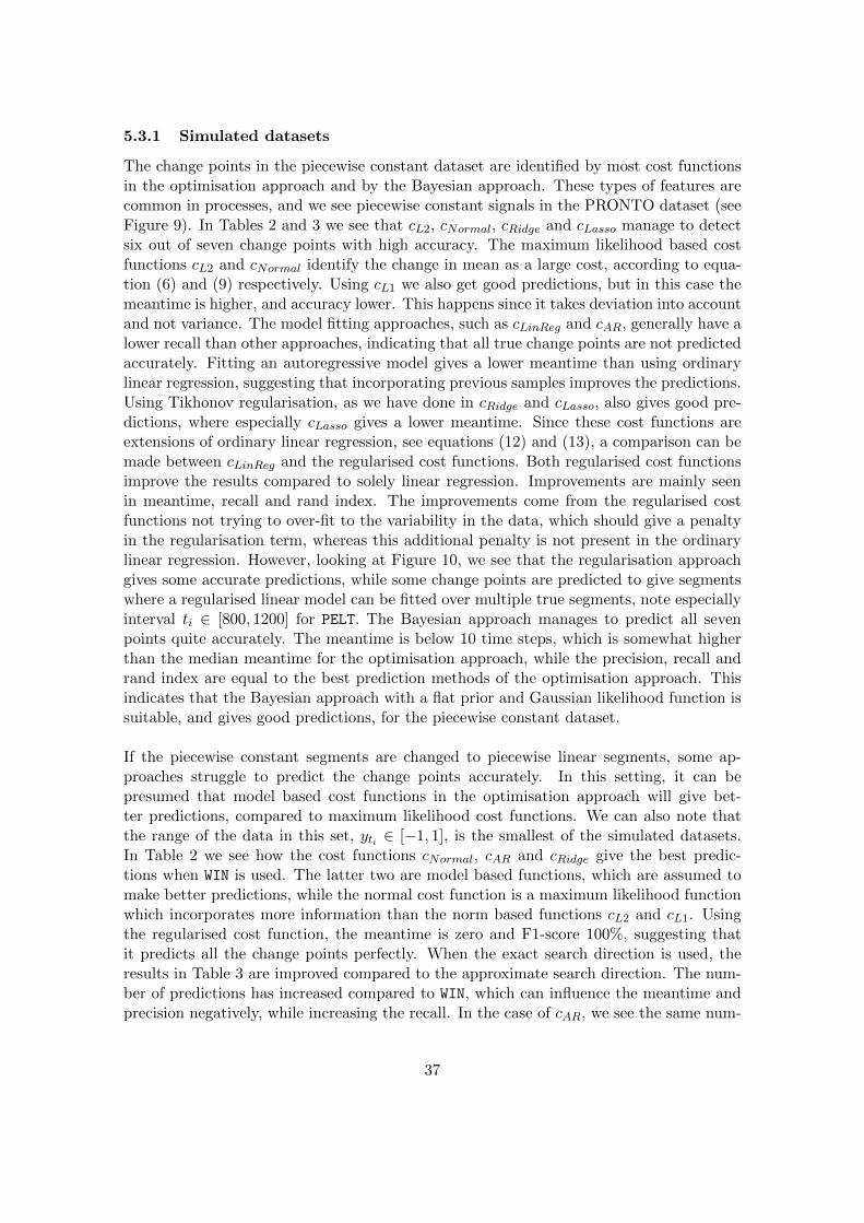
5.3.1 Simulated datasets

The change points in the piecewise constant dataset are identified by most cost functionsin the optimisation approach and by the Bayesian approach. These types of features arecommon in processes, and we see piecewise constant signals in the PRONTO dataset (seeFigure 9). In Tables 2 and 3 we see that cL2, cNormal, cRidge and cLasso manage to detectsix out of seven change points with high accuracy. The maximum likelihood based costfunctions cL2 and cNormal identify the change in mean as a large cost, according to equa-tion (6) and (9) respectively. Using cL1 we also get good predictions, but in this case themeantime is higher, and accuracy lower. This happens since it takes deviation into accountand not variance. The model fitting approaches, such as cLinReg and cAR, generally have alower recall than other approaches, indicating that all true change points are not predictedaccurately. Fitting an autoregressive model gives a lower meantime than using ordinarylinear regression, suggesting that incorporating previous samples improves the predictions.Using Tikhonov regularisation, as we have done in cRidge and cLasso, also gives good pre-dictions, where especially cLasso gives a lower meantime. Since these cost functions areextensions of ordinary linear regression, see equations (12) and (13), a comparison can bemade between cLinReg and the regularised cost functions. Both regularised cost functionsimprove the results compared to solely linear regression. Improvements are mainly seenin meantime, recall and rand index. The improvements come from the regularised costfunctions not trying to over-fit to the variability in the data, which should give a penaltyin the regularisation term, whereas this additional penalty is not present in the ordinarylinear regression. However, looking at Figure 10, we see that the regularisation approachgives some accurate predictions, while some change points are predicted to give segmentswhere a regularised linear model can be fitted over multiple true segments, note especiallyinterval ti ∈ [800, 1200] for PELT. The Bayesian approach manages to predict all sevenpoints quite accurately. The meantime is below 10 time steps, which is somewhat higherthan the median meantime for the optimisation approach, while the precision, recall andrand index are equal to the best prediction methods of the optimisation approach. Thisindicates that the Bayesian approach with a flat prior and Gaussian likelihood function issuitable, and gives good predictions, for the piecewise constant dataset.

If the piecewise constant segments are changed to piecewise linear segments, some ap-proaches struggle to predict the change points accurately. In this setting, it can bepresumed that model based cost functions in the optimisation approach will give bet-ter predictions, compared to maximum likelihood cost functions. We can also note thatthe range of the data in this set, yti ∈ [−1, 1], is the smallest of the simulated datasets.In Table 2 we see how the cost functions cNormal, cAR and cRidge give the best predic-tions when WIN is used. The latter two are model based functions, which are assumed tomake better predictions, while the normal cost function is a maximum likelihood functionwhich incorporates more information than the norm based functions cL2 and cL1. Usingthe regularised cost function, the meantime is zero and F1-score 100%, suggesting thatit predicts all the change points perfectly. When the exact search direction is used, theresults in Table 3 are improved compared to the approximate search direction. The num-ber of predictions has increased compared to WIN, which can influence the meantime andprecision negatively, while increasing the recall. In the case of cAR, we see the same num-

37

ber of predictions in the two tables, and the meantime is somewhat lower when PELT isused. On the other hand, the precision and recall are lower. This suggests that in generalthe predictions are more accurate, while one prediction is outside the allowed margin forprecision and recall, causing a decrease in the meantime. The Bayesian approach predictsonly two points, where one is the artificial change point at the end of the data. In Fig-ure 20 (in Appendix A) we see how the distinct drop in value at ti = 300 gives a strongindication while the other do not. This could be due to the range of the data, and the notas significant change in slope will not be perceived as a change point.

If only the variance changes, then it is natural to expect approaches which incorporate thevariance to give the best predictions. The Bayesian approach includes information con-cerning change in variance in the Gaussian likelihood function, where a change in variancecan mean a change in distribution and therefor a change point. The maximum likelihoodbased cost functions cL2 and cL1 do not incorporate the variance directly, while the ex-tended version cNormal does, see equation (9). In Table 2 we see how this cost functiongives the most accurate predictions, with AE = 0 and a meantime of 22 time steps, whichis the lowest of all cost functions. We can also note how cLasso does not identify anychange points (even with zero penalty) in this setting, except the artificial one at the end,which suggests that it fits one model for the entirety of the data. In Figure 5 (top) wesee how cNormal predicts four of the change points accurately, while the remainder arenot accurate predictions. This can arguably be due to the features in the data. Somechange points do not have as distinct change points, as defined in Definition 1. The lackof distinctness in the change points causes the change point detection to be difficult, as thechange is not significant. In Figure 5 we also see that this correlates with the predictionsmade by the Bayesian approach, where four change points are identified. To extend theinvestigation, the algorithms can predict fewer change points and see if these agree more.In Figure 17 we see the predictions made by a few algorithms and the Bayesian approach.The predictions made using the Bayesian approach and cNormal give similar predictions,while other cost functions give different predictions. This confirms that both the Bayesianapproach and the cNormal cost function incorporate variance changes in an effective way,while other cost functions do not.

38

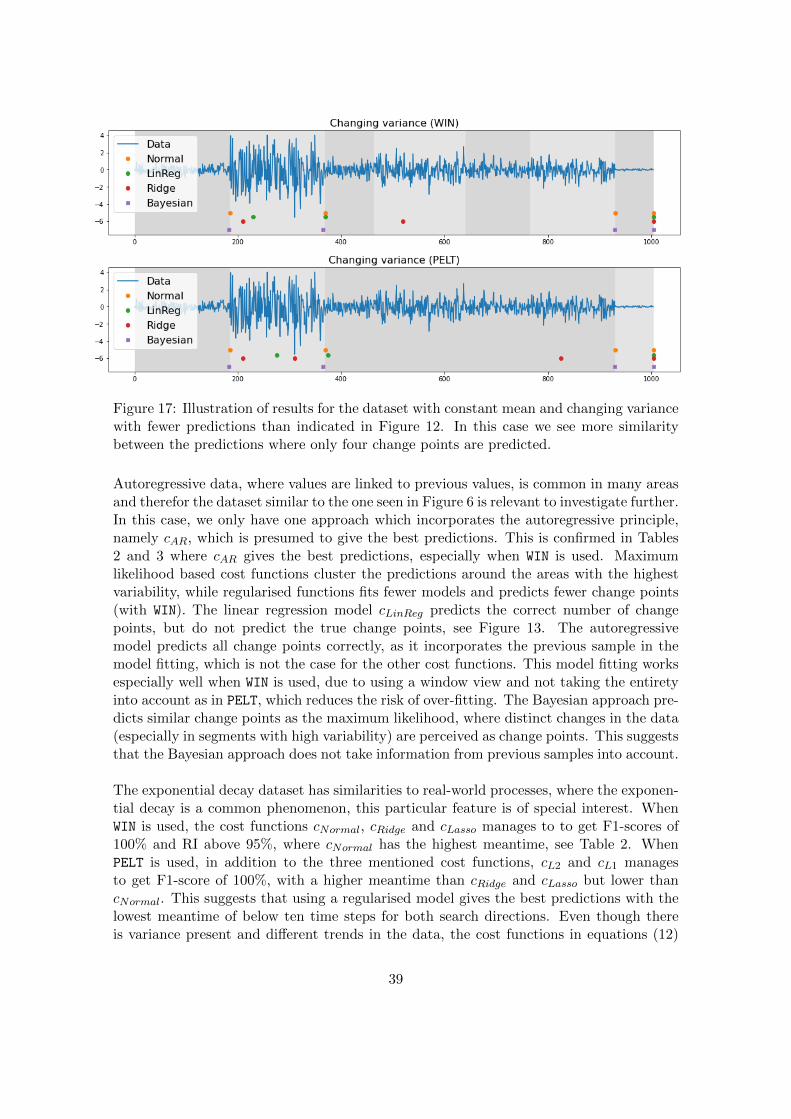
Figure 17: Illustration of results for the dataset with constant mean and changing variancewith fewer predictions than indicated in Figure 12. In this case we see more similaritybetween the predictions where only four change points are predicted.

Autoregressive data, where values are linked to previous values, is common in many areasand therefor the dataset similar to the one seen in Figure 6 is relevant to investigate further.In this case, we only have one approach which incorporates the autoregressive principle,namely cAR, which is presumed to give the best predictions. This is confirmed in Tables2 and 3 where cAR gives the best predictions, especially when WIN is used. Maximumlikelihood based cost functions cluster the predictions around the areas with the highestvariability, while regularised functions fits fewer models and predicts fewer change points(with WIN). The linear regression model cLinReg predicts the correct number of changepoints, but do not predict the true change points, see Figure 13. The autoregressivemodel predicts all change points correctly, as it incorporates the previous sample in themodel fitting, which is not the case for the other cost functions. This model fitting worksespecially well when WIN is used, due to using a window view and not taking the entiretyinto account as in PELT, which reduces the risk of over-fitting. The Bayesian approach pre-dicts similar change points as the maximum likelihood, where distinct changes in the data(especially in segments with high variability) are perceived as change points. This suggeststhat the Bayesian approach does not take information from previous samples into account.

The exponential decay dataset has similarities to real-world processes, where the exponen-tial decay is a common phenomenon, this particular feature is of special interest. WhenWIN is used, the cost functions cNormal, cRidge and cLasso manages to to get F1-scores of100% and RI above 95%, where cNormal has the highest meantime, see Table 2. WhenPELT is used, in addition to the three mentioned cost functions, cL2 and cL1 managesto get F1-score of 100%, with a higher meantime than cRidge and cLasso but lower thancNormal. This suggests that using a regularised model gives the best predictions with thelowest meantime of below ten time steps for both search directions. Even though thereis variance present and different trends in the data, the cost functions in equations (12)

39

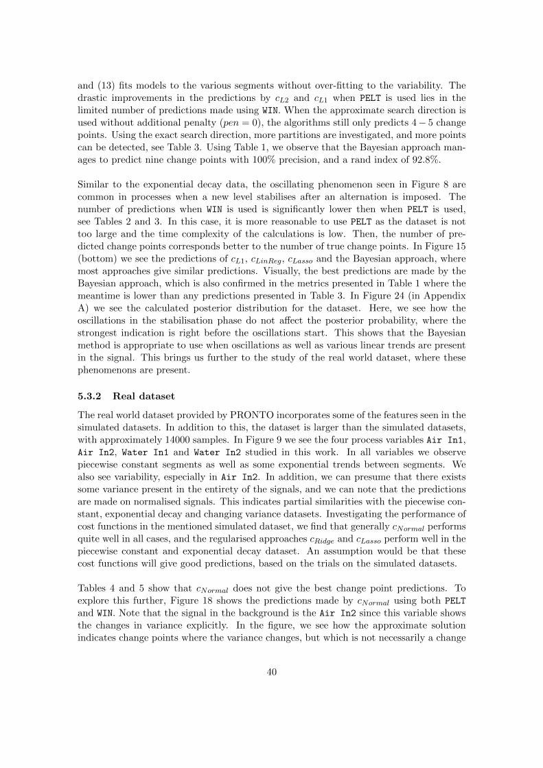
and (13) fits models to the various segments without over-fitting to the variability. Thedrastic improvements in the predictions by cL2 and cL1 when PELT is used lies in thelimited number of predictions made using WIN. When the approximate search direction isused without additional penalty (pen = 0), the algorithms still only predicts 4− 5 changepoints. Using the exact search direction, more partitions are investigated, and more pointscan be detected, see Table 3. Using Table 1, we observe that the Bayesian approach man-ages to predict nine change points with 100% precision, and a rand index of 92.8%.

Similar to the exponential decay data, the oscillating phenomenon seen in Figure 8 arecommon in processes when a new level stabilises after an alternation is imposed. Thenumber of predictions when WIN is used is significantly lower then when PELT is used,see Tables 2 and 3. In this case, it is more reasonable to use PELT as the dataset is nottoo large and the time complexity of the calculations is low. Then, the number of pre-dicted change points corresponds better to the number of true change points. In Figure 15(bottom) we see the predictions of cL1, cLinReg, cLasso and the Bayesian approach, wheremost approaches give similar predictions. Visually, the best predictions are made by theBayesian approach, which is also confirmed in the metrics presented in Table 1 where themeantime is lower than any predictions presented in Table 3. In Figure 24 (in AppendixA) we see the calculated posterior distribution for the dataset. Here, we see how theoscillations in the stabilisation phase do not affect the posterior probability, where thestrongest indication is right before the oscillations start. This shows that the Bayesianmethod is appropriate to use when oscillations as well as various linear trends are presentin the signal. This brings us further to the study of the real world dataset, where thesephenomenons are present.

5.3.2 Real dataset

The real world dataset provided by PRONTO incorporates some of the features seen in thesimulated datasets. In addition to this, the dataset is larger than the simulated datasets,with approximately 14000 samples. In Figure 9 we see the four process variables Air In1,Air In2, Water In1 and Water In2 studied in this work. In all variables we observepiecewise constant segments as well as some exponential trends between segments. Wealso see variability, especially in Air In2. In addition, we can presume that there existssome variance present in the entirety of the signals, and we can note that the predictionsare made on normalised signals. This indicates partial similarities with the piecewise con-stant, exponential decay and changing variance datasets. Investigating the performance ofcost functions in the mentioned simulated dataset, we find that generally cNormal performsquite well in all cases, and the regularised approaches cRidge and cLasso perform well in thepiecewise constant and exponential decay dataset. An assumption would be that thesecost functions will give good predictions, based on the trials on the simulated datasets.

Tables 4 and 5 show that cNormal does not give the best change point predictions. Toexplore this further, Figure 18 shows the predictions made by cNormal using both PELT

and WIN. Note that the signal in the background is the Air In2 since this variable showsthe changes in variance explicitly. In the figure, we see how the approximate solutionindicates change points where the variance changes, but which is not necessarily a change

40

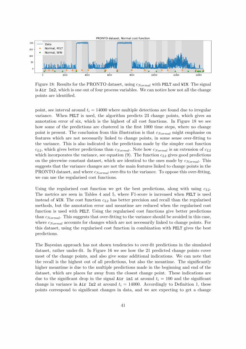
Figure 18: Results for the PRONTO dataset, using cNormal with PELT and WIN. The signalis Air In2, which is one out of four process variables. We can notice how not all the changepoints are identified.

point, see interval around ti = 14000 where multiple detections are found due to irregularvariance. When PELT is used, the algorithm predicts 23 change points, which gives anannotation error of six, which is the highest of all cost functions. In Figure 18 we seehow some of the predictions are clustered in the first 1000 time steps, where no changepoint is present. The conclusion from this illustration is that cNormal might emphasise onfeatures which are not necessarily linked to change points, in some sense over-fitting tothe variance. This is also indicated in the predictions made by the simpler cost functioncL2, which gives better predictions than cNormal. Note how cNormal is an extension of cL2

which incorporates the variance, see equation (9). The function cL2 gives good predictionson the piecewise constant dataset, which are identical to the ones made by cNormal. Thissuggests that the variance changes are not the main features linked to change points in thePRONTO dataset, and where cNormal over-fits to the variance. To oppose this over-fitting,we can use the regularised cost functions.

Using the regularised cost function we get the best predictions, along with using cL2.The metrics are seen in Tables 4 and 5, where F1-score is increased when PELT is usedinstead of WIN. The cost function cL2 has better precision and recall than the regularisedmethods, but the annotation error and meantime are reduced when the regularised costfunction is used with PELT. Using the regularised cost functions give better predictionsthan cNormal. This suggests that over-fitting to the variance should be avoided in this case,where cNormal accounts for changes which are not necessarily linked to change points. Forthis dataset, using the regularised cost function in combination with PELT gives the bestpredictions.

The Bayesian approach has not shown tendencies to over-fit predictions in the simulateddataset, rather under-fit. In Figure 16 we see how the 21 predicted change points covermost of the change points, and also give some additional indications. We can note thatthe recall is the highest out of all predictions, but also the meantime. The significantlyhigher meantime is due to the multiple predictions made in the beginning and end of thedataset, which are places far away from the closest change point. These indications aredue to the significant drop in the signal Air in1 at around ti = 100 and the significantchange in variance in Air In2 at around ti = 14000. Accordingly to Definition 1, thesepoints correspond to significant changes in data, and we are expecting to get a change

41

point here in the case when they will be sensitive to changes in mean or variance. In thiscase the Bayesian approach incorporates both. If the predictions in the beginning and endof time intervals would have been correct, the predictions of the Bayesian method wouldyield a good prediction of most of the true change points present in the PRONTO dataset.

In Tables 6 and 7 we see how different regularisation parameters can affect the prediction.The tables show that selecting an appropriate regularisation constant is of importance. Inthe results presented in Table 2-5 the constant γ = 1 has been used, where Tables 6 and 7present other possible values for γ. It is evident that the investigation is not exact, andindicates that different parameter choices for γ give different predictions. In contrast tosimply selecting different values, other methods to estimate an appropriate value can beused, such as iterative approximation. These extended algorithms are not covered in thiswork, but could be of interest for future work.

5.4 User interaction

To make the explored unsupervised CPD approaches user friendly and more effective,we want to explore the possibilities of incorporating user feedback or prior knowledge.This can either be done via changes in settings of the unsupervised approaches or afterpredictions have been made. The two approaches have different modifications which canbe made to alter the predictions. In the upcoming sections these possibilities are discussedwith respect to the optimisation approach and the Bayesian approach individually.

5.4.1 Optimisation approach

After the discussion of the results in previous sections, a natural way to affect the pre-dicted change points is to select an appropriate cost function. If the data contains certainfeatures, as explored in the simulated datasets, we can chose an appropriate cost functionaccording to the underlying assumptions and function formulation. Alternatively, we knowwhich type of change point we want to detect, and therefor can choose a cost functionwhich is sensitive to specific changes in the data.

A parameter which can be changed to affect the number of predictions is the penalty.This constant can be estimated by performing multiple estimations and selecting thepenalty level which gives the best metrics. If this was not sought after, the constant canbe either increased to reduce the number of predictions or decreased to possibly3 increasethe number of predictions. A user friendly implementation would first estimate the bestpenalty level and perform CPD. This penalty can then be altered by the user, if the resultsare not satisfactory, to give another prediction.

If the unsupervised algorithm gives a generally good prediction of the change points, butthere are domain specific change points present (see Definition 2), the predicted points canbe altered. A change point could either be added or removed given the prediction madeby the unsupervised algorithm. It should be noted that this will be a tedious task for a

3If the penalty is zero, the penalty term cannot be reduced further and therefor not generate morepredictions.

42

large number of domain specific change points, and additional solutions will be requiredto automate such tasks.

5.4.2 Bayesian approach

For the Bayesian approach we can make appropriate choices for prior and likelihood func-tion, similar to the choice of cost function in the optimisation approach. The prior containsinformation about the distance between change points while the likelihood function con-tains information about the segments. By choosing these according to the available data,the accuracy of the predictions can be increased. An example is to use a discrete geometricdistribution as a prior, instead of a flat prior, if there is knowledge of the change pointsbeing equally spaced.

A parameter change can be done to the peak selection criterion. As default, the peakselection can have a setting similar to the one used in this work, to give a first predictionof the change points. If the results are not satisfactory, the user could try to change theconfidence level or distance parameters and see if this gives other predictions. If furtheralternations are necessary, a predictions can either be added or removed using the sameprinciple as the optimisation approach.

In addition to the presented user interaction, the use of probabilities can incorporateadditional probability distributions. When the posterior distribution is calculated, but anarea which should contain a change point does not have a high probability, the posteriordistribution can be further joint with a domain specified distribution. This means thatif a user knows approximately where a change point is present, a probability distributionwith mean and variance according to the users’ expectation can be found and joined withthe calculated posterior distribution. This means that the posterior distribution of changepoints can incorporate the information from users without being recalculated.

5.5 Future work

As the application area of change point detection is wide and options of how to predictthese points are many, this work does not cover all relevant topics. Future work can bepursued in areas such as defining new cost functions linked to specific feature identificationusing the optimisation approach, or other prior and likelihood function for the Bayesianapproach. By making strategic choices, and trying to incorporate information about thedata or sought after change points, the accuracy in the predictions can be increased. Theapplication area can also be widened by studying the online version of change point detec-tion, whereas this work has focused on the offline version. Potentially, similar comparisonscan be made for the online CPD where aspects of this work can be implemented.

This work has focused on simple implementations of Tikhonov regularisation, but there arenumerous other options. This work has studied a selected constant as the regularisationparameter γ in equations (12) and (13), but there is potential in iterative updates of the pa-rameter [21, 22]. Other regularisation methods which can be studied include the balancingprinciple [25], L-curve or S-curve methods [33] and randomised SVD methods [34]. Totalvariation regularisation can also be applied, which has been applied for denoising data [35].

43

In addition to the theoretical aspects, the usability in industry settings can be studiedfurther. This work has focused on comparing the usability in industries, where furtherinvestigations can be pursued in terms of change point usage. A relevant question is: howcan the production in industrial processes benefit from the predicted change points in theprocess data? Ideas could be to use the change points to identify production phases or forsyncing phases in chemical processes in order to identify anomalies.

6 Conclusion

This work has studied two unsupervised algorithms for detecting change points. Oneapproach is formulated as an optimisation problem while the other is based on Bayesianstatistics. The study has found that the algorithms are affected by the features in theunderlying data, where both simulated and real world data have been examined. In theoptimisation approach, the choice of cost function can affect the predictions made bythe algorithm, where these functions are strongly linked to the type of features beingdetected as change points. A new type of cost function has been introduced, which usesTikhonov regularisation. The Bayesian approach uses prior knowledge on the distancebetween change points and a likelihood function with information about the segments inorder to predict the probability of a time point being a change point. To this day, thetwo mentioned approaches have not been compared, nor has the regularisation been usedfor change point detection previously. In addition to this, the possibility to incorporateuser feedback has been explored, where both approaches are able to incorporate userknowledge and corrections post prediction. This sheds light on the potential usabilityoutside of academia. The importance of change point detection becomes more and moreimportant as datasets increase in size, where these unsupervised detection algorithms canhelp users process the data in order to draw conclusions.

44

References

[1] E.S. Page. Continuous inspection schemes. Biometrika, 41, 1954.

[2] E.S. Page. A test for a change in a parameter occurring at an unknown point.Biometrika, 42, 1955.

[3] L. Oudreb C. Truonga and N. Vayatisa. Selective review of offline change pointdetection methods. 2020.

[4] M. Eriksson. Change point detection with applications to wireless sensor networks.Digital Comprehensive Summaries of Uppsala Dissertations from the Faculty of Sci-ence and Technology, 2019.

[5] A. Lung-Yut-Fong Z. Harchaoui, F. Vallet and O. Cappe. A regularized kernel-basedapproach to unsupervised audio segmentation. International Conference on Acoustics,Speech and Signal Processing (ICASSP), pages 1665–1668, 2009.

[6] M. Lavielle and G. Teyssiere. Adaptive detection of multiple change-points in assetprice volatility. In Long-Memory in Economics, pages 129–156, 2007.

[7] C. Levy-Leduc A. Lung-Yut-Fong and O. Cappe. Distributed detection of change-points in high-dimensional network trafic data. Statistics and Computing, 22:485–496,2012.

[8] B. Duarte and P. Saraiva. Change point detection for quality monitoring of chem-ical processes. In A. Kraslawski and I. Turunen, editors, European Symposium onComputer Aided Process Engineering-13, volume 14 of Computer Aided ChemicalEngineering, pages 401–406. Elsevier, 2003.

[9] P. Fearnhead. Exact and efficient bayesian inference for multiple changepoint. Statis-tics and Computing, 16:203–213, 06 2006.

[10] C.M. Bishop. Pattern Recognition and Machine Learning. Springer, 2006.

[11] S. B. Kotsiantis. Supervised machine learning: A review of classification techniques.Informatica, 31:249–268, 2007.

[12] I. Goodfellow, Y. Bengio, and A. Courville. Deep Learning. MIT Press, 2016. http://www.deeplearningbook.org.

[13] G.J.J. van den Burg and C.K.I. Williams. An evaluation of change point detectionalgorithms. 2020.

[14] V. Jandhyala, S.B. Fotopoulos, I. Macneill, and P. Liu. Inference for single andmultiple change-points in time series. Journal of Time Series Analysis, 34:423–446,07 2013.

[15] C. Truong et al. Ruptures. https://github.com/deepcharles/ruptures. Accessed:2021-01-11.

45

[16] J. Kulick. Bayesian change point detection repository. https://github.com/

hildensia/bayesian_changepoint_detection. Accessed: 2021-01-11.

[17] B. Mirko. Contrast and change mining. WIREs Data Mining and Knowledge Discov-ery, 1(3):215–230, 2011.

[18] H. Kashima-H. Kubo S. Hido, T. Ide and H. Matsuzawa. Unsupervised change anal-ysis using supervised learning. 2008.

[19] S. Aminikhanghahi and D. Cook. A survey of methods for time series change pointdetection. Knowledge and information systems, 51:339–367.

[20] V.Y. Arsenin A.N. Tikhonov. Solutions of ill-posed problems. Wiley, 1977.

[21] V.V. Stepanov-A.G. Yagola A.N. Tikhonov, A. Goncharsky. Numerical Methods forthe Solution of Ill-Posed Problems. Springer, 1995.

[22] A. Neubauer B. Kaltenbacher and O. Scherzer. Iterative Regularization Methods forNonlinear Ill-Posed Problems. De Gruyter, 2008.

[23] M.Yu. Kokurin A.B. Bakushinsky. Iterative Methods for Approximate Solution ofInverse Problems. Springer, 2004.

[24] M.V. Klibanov L. Beilina. Approximate Global Convergence and Adaptivity for Co-efficient Inverse Problems. Springer, 2012.

[25] L.Beilina. Numerical analysis of least squares and perceptron learning for classifica-tion problems. Open Journal of Discrete Applied Mathematics, page 30 – 49, 2020.

[26] A.K.M.E. Saleh, M. Arashi, and B.M.G. Kibria. Theory of Ridge Regression Estima-tion with Applications. Wiley Series in Probability and Statistics. Wiley, 2019.

[27] Z. Ivezic, A.J. Connolly, J.T. VanderPlas, and A. Gray. Statistics, Data Mining,and Machine Learning in Astronomy: A Practical Python Guide for the Analysisof Survey Data. Princeton Series in Modern Observational Astronomy. PrincetonUniversity Press, 2014.

[28] T. Bayes. An essay towards solving a problem in the doctrine of chances. 1763.Communicated by Mr. Price, in a letter to John Canton.

[29] A. Stief, R. Tan, Y. Cao, J.R. Ottewill, N.F. Thornhill, and J. Baranowski. A het-erogeneous benchmark dataset for data analytics: Multiphase flow facility case study.Journal of Process Control, 79:41–55, 2019.

[30] Y. Cao A. Stief, R. Tan and J.R. Ottewill. Pronto heterogeneous benchmark dataset,2019. data retrieved from Zenodo, https://doi.org/10.5281/zenodo.1341583.

[31] R. Tavenard. Tslearn piecewise aggregate pproximation (PAA). https:

//tslearn.readthedocs.io/en/stable/gen_modules/piecewise/tslearn.

piecewise.PiecewiseAggregateApproximation.html#tslearn.piecewise.

PiecewiseAggregateApproximation. Accessed: 2021-03-31.

46

[32] The SciPy community. Scipy find peaks. https://docs.scipy.org/doc/scipy/

reference/generated/scipy.signal.find_peaks.html. Accessed: 2021-03-31.

[33] K. Niinimaki, M. Hanhela, and V. Kolehmainen. Parameter selection in dynamiccontrast-enhanced magnetic resonance tomography. Springer Proceedings in Mathe-matics Statistics, 328, 2020.

[34] K. Ito and B. Jin. Regularized linear inversion with randomized singular value decom-position. In L. Beilina, M. Bergounioux, M. Cristofol, A. Da Silva, and A. Litman,editors, Mathematical and Numerical Approaches for Multi-Wave Inverse Problems,pages 45–72, Cham, 2020. Springer International Publishing.

[35] L. Condat. A direct algorithm for 1d total variation denoising. IEEE Signal ProcessingLetters, 20(11):1054–1057, 2013.

47

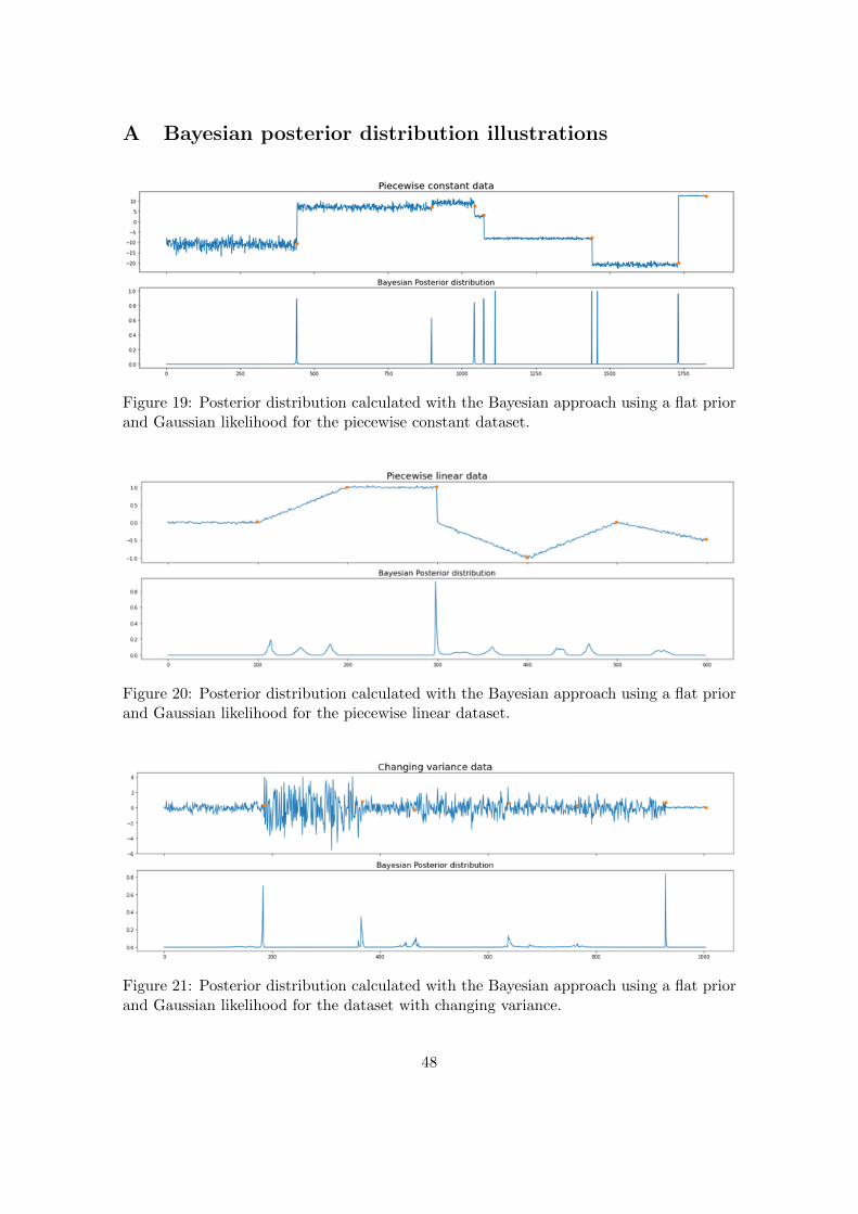
A Bayesian posterior distribution illustrations

Figure 19: Posterior distribution calculated with the Bayesian approach using a flat priorand Gaussian likelihood for the piecewise constant dataset.

Figure 20: Posterior distribution calculated with the Bayesian approach using a flat priorand Gaussian likelihood for the piecewise linear dataset.

Figure 21: Posterior distribution calculated with the Bayesian approach using a flat priorand Gaussian likelihood for the dataset with changing variance.

48

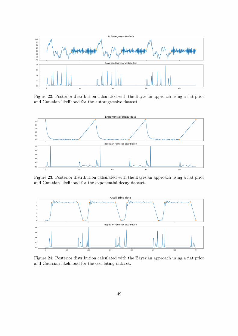
Figure 22: Posterior distribution calculated with the Bayesian approach using a flat priorand Gaussian likelihood for the autoregressive dataset.

Figure 23: Posterior distribution calculated with the Bayesian approach using a flat priorand Gaussian likelihood for the exponential decay dataset.

Figure 24: Posterior distribution calculated with the Bayesian approach using a flat priorand Gaussian likelihood for the oscillating dataset.

49

B Code

Code for all experiments can be retrieved at:https://github.com/geddar/Interactive-change-point-detection.These files include implementations from other repositories, presented below. The repos-itory includes a README file with all information needed for reproducing the experimentsfound in this work.

Code for the optimisation approach can be retrieved at:https://github.com/deepcharles/ruptures.

Code for implementation of the Bayesian approach can be retrieved at:https://github.com/hildensia/bayesian_changepoint_detection.

50