INTERACTIVE COMPUTATIONAL TOOL FOR SIMULATION OF … · 2018-07-24 · Newmark integration (δ=0.25, γ=0.5, ... versus nodal displacement vector (Fig.5) for cross sections located

ASME Early Career Technical Journal 2010 ASME Early Career Technical Conference, ASME ECTC

October 1-2, 2010, GA Tech, Atlanta, Georgia, USA

INTERACTIVE COMPUTATIONAL TOOL FOR SIMULATION OF DYNAMIC RESPONSE AND DAMAGE IN COMPOSITE STRUCTURES

Tezeswi, P., Tadepalli, Research Associate Department of Mechanical Engineering,

Composite Structures and Nano-Engineering Research Group,

The University of Mississippi University, MS-38677, USA

Christopher, L., Mullen, Associate Professor Department of Civil Engineering,

Composite Structures and Nano-Engineering Research Group,

The University of Mississippi University, MS-38677, USA

ABSTRACT An interactive computational simulation tool has been developed, that is useful for assessing modal vibration test results and estimating damage in composite structures. A graphical user interface has been implemented as a simple template for performing a variety of time domain based dynamic and nonlinear analyses. The tool incorporates a complementary finite element procedure which enables tracking of complex flexural damage states for beam-columns. The linear dynamic simulation capabilities are validated using ideal SDOF and MDOF systems and applied towards rapid structural property identification of portal frames made of mechanically joined pultruded flat hybrid composites. Damage simulation capabilities are illustrated for an ideal cantilever beam loaded to collapse. Keywords: Vibration; Plastic deformation; Finite Element Analysis; Non-destructive testing INTRODUCTION

An interactive computational simulation tool called FESIM has been developed for composite structures dynamic response analysis which permits an interface between experimental modal analysis (EMA) and finite element (FE) simulation of damage. The tool is useful for advanced undergraduate/graduate instruction and has been developed in a computational framework that enables a variety of research activities. The simulation framework includes a variety of time domain based linear and nonlinear dynamic analyses, which can initiate from either experimental modal analysis or FE formulation for structural systems made of advanced composite materials.

A 2-D frame element has been incorporated for demonstrating linear dynamic simulation capabilities for composite frame structural systems. The programming framework, however, admits extension to nonlinear dynamic behavior of 3D frame, solid, and shell systems. A concise graphical user interface (GUI) [1] (Fig. 1) has been created to enable simple and direct input by the user

including structural property matrices for small instructional problems involving single degree of freedom (SDOF) models and up to six DOF through screen input to the interface. Large multi-DOF (MDOF) models are accommodated through simple pre-processing steps easily handled using the programming environment. Several experimental and FE simulation studies dealing mainly with linear elastic response of pultruded composites have been reported in the literature.

Davalos et al. [2] have shown that pultruded sections have material architectures that can be simulated as laminated configurations. A linear elastic laminate mechanics analysis is described and results are compared with FE analyses. Ghiringhelli et al. [3] have developed a 3-D beam which is suitable for use within a linear framework of analysis. Nori et al. [4] have conducted experimental characterization and FE analysis of glass-graphite/epoxy pultruded hybrid composites in axial and flexural modes of vibration. Various combinations and volume fractions of graphite and glass fibers were tested for dynamic response, and results were compared with FE simulations.

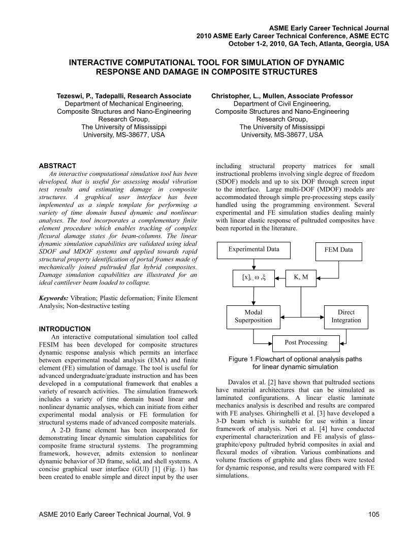
Experimental Data FEM Data

[x]i , ω ,ξ K, M

Modal Superposition

Direct Integration

Post Processing

Figure 1.Flowchart of optional analysis paths for linear dynamic simulation

ASME 2010 Early Career Technical Journal, Vol. 9 105

Nonlinear macro- and micro-mechanical constitutive models in laminated composites have been studied extensively. Haj-Ali and Kilic [5] have compared static experimental tests with FE simulations of nonlinear elastic material response of pultruded sections using a micro-mechanical modeling approach. Kilic and Haj-Ali [6] extended their approach to simulation of nonlinear inelastic material response by writing a user material subroutine which incorporated their micro-mechanical model into the ABAQUS layered shell element. In this way the authors were able to simulate the progression of damage around a notch in a pultruded FRP composite. Ganapathi et al. [7] have conducted linear and nonlinear vibration analyses wherein geometric nonlinearity was considered but material nonlinearity was not considered.

In the above mentioned studies, either shell or solid elements were used to model the composites. In the present study a framework is demonstrated that enables linear dynamic response and nonlinear damage modeling that is facilitated by a section based beam-column finite element. Nonlinear dynamic response is also demonstrated for a SDOF system. The simulations are validated with experimental modal analysis (EMA) results for portal frames, and can further be employed to predict the properties of other hypothetical combinations that were not pultruded.

VALIDATION OF TIME INTEGRATION ALGORITHMS FOR LINEAR SDOF AND MDOF SYSTEMS

FESIM computes the response to harmonic loading using two methods: 1) direct integration using the Generalized Newmark method [8, 9], and 2) mode superposition using impulse response functions [10].

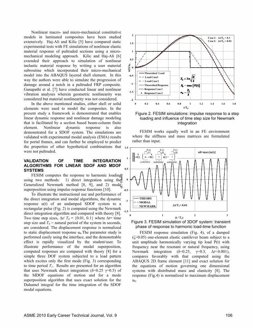
To illustrate the instructional use and performance of the direct integration and modal algorithms, the dynamic response u(t) of an undamped SDOF system to a rectangular pulse (Fig. 2) is computed using the Newmark direct integration algorithm and compared with theory [8]. Two time step sizes, ∆t/ T0 = {0.01, 0.1} where ∆t= time step size and T0 = natural period of the system in seconds, are considered. The displacement response is normalized to static displacement response u0.The parameter study is performed easily using the interface, and the demonstrable effect is rapidly visualized by the student/user. To illustrate performance of the modal superposition, computed responses are compared with theory [8] for a simple three DOF system subjected to a load pattern which excites only the first mode (Fig. 3) corresponding to time period T1. Results are presented for an algorithm that uses Newmark direct integration (δ=0.25 γ=0.5) of the MDOF equations of motion and for a mode superposition algorithm that uses exact solution for the Duhamel integral for the time integration of the SDOF modal equations.

FESIM works equally well in an FE environment

where the stiffness and mass matrices are formulated rather than input.

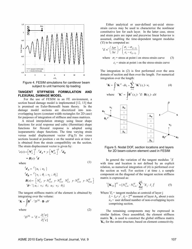
FESIM response simulation (Fig. 4), of a damped

(ζ=0.05) one-element elastic cantilever beam subject to a unit amplitude harmonically varying tip load P(t) with frequency near the resonant or natural frequency, using Newmark integration (δ=0.25, γ=0.5, ∆t=0.001), compares favorably with that computed using the ABAQUS 2D frame element [11] and exact solution for the equations of motion governing one dimensional systems with distributed mass and elasticity [8]. The response (Fig.4) is normalized to maximum displacement u0.

-2

-1.5

-1

-0.5

0

0.5

1

1.5

2

0 0.2 0.4 0.6 0.8 1 1.2 1.4 1.6 1.8

u(t

)/u

0

t/T0

Theoretical Load

Load Case1

Load Case 2

Theoretical Response

Response Case 1

Response Case 2

Case 1: t/T0 = 0.1Case 2: t/T0 = 0.01

-1.5

-1

-0.5

0

0.5

1

1.5

0 1 2 3

(U /

Um

ax)

(t / T1)

THEORYMODALNEWMARK

u0=max{u(t)}

t/T1= 0.01

Figure 3. FESIM simulation of 3DOF system: transient phase of response to harmonic load-time function

Figure 2. FESIM simulations: impulse response to a step loading and influence of time step size for Newmark

integration


TANGENT STIFFNESS FORMULATION AND FLEXURAL DAMAGE MODEL

For the use of FESIM in an FE environment, a section based damage model is implemented [12, 13] that is premised on Euler-Bernoulli beam theory. In the damage model sections are discretized into non-overlapping layers (constant width rectangles for 2D case) for purposes of integration of stiffness and mass matrices. A mixed interpolation strategy using linear shape functions for axial response and cubic (Hermitian) shape functions for flexural response is adopted using isoparametric shape functions. The time varying strain versus nodal displacement vector (Fig.5) for cross sections located at position x on the neutral axis at time t is obtained from the strain compatibility on the section. The strain displacement vector is given by:

T T

, ,

1 2

1 1 2 2

1, 1, 3, 2, 2, 4,

( )

( )

where

;

; ; ;

( )

t L Hx xx

L H H L H Hx xx xx x xx xx

t tx y

tx

t t u u

t t v v

x N y N y N N y N y N

N NA B

A

B

d + d

= B d

d

d

B

td= t{ u1 ; v1; θ1; u2; v2; θ2} The tangent stiffness matrix of the element is obtained by integrating over the volume:

where

[ ]

[ ]

t T t NL

V

tt NL t

t

D dV

D E

K B B

(2)

Either analytical or user-defined uni-axial stress-strain curves may be used to characterize the nonlinear constitutive law for each layer. In the latter case, stress and strain pairs are input and piecewise linear behavior is assumed, enabling the time-dependent tangent modulus (tE) to be computed as:

( 1)

( 1)

where = stress at point i on stress-strain curve

= strain at point i on the stress-strain curve

i it t t

i i

i

i

E

(3)

The integration in (2) is first performed over the area domain of section and then over the length. For numerical integration over the length:

2

11

( )t t A t ii i

iL

dx x w

K K K (4)

where ( ) ( )t i T ti i

A

x E x dA K B B

In general the variation of the tangent modulus tE with time and location is not defined by an explicit relation, so numerical integration of (4) is performed over the section as well. For section i at time t, a sample component on the diagonal of the tangent section stiffness matrix is expressed as:

22 1, 1,1

[ ]nA

t Ai H H t ixx xx j j

j

N N E I

K (5)

Where tEj = tangent modulus at centroid of layer j Ij = Ij0+y2. Aj = 2nd moment of layer Aj, about z-axis nA = user defined number of non-overlapping layers comprising section.

The remaining components may be expressed in

similar fashion. Once assembled, the element stiffness matrix tK , is used to construct the global stiffness matrix tKG for the entire structure, based on element connectivity.

t/T1

(1)

Figure 5. Nodal DOF, section locations and layers for 2D beam-column element used in FESIM

Figure 4. FESIM simulations for cantilever beam subject to unit harmonic tip loading

-1.5

-1

-0.5

0

0.5

1

1.5

0 2 4 6 8 10 12

U(t

)/ U

max

ABAQUS-NEWMARK

FESIM-NEWMARK

P(t)


The lumped mass matrix for a beam is often sufficiently accurate for most applications. However, for a consistent mass matrix, the integration is carried out in a manner similar to the tangent stiffness, i.e. for section i at time t:

t T t

VdV M N N (6)

Where t = time varying mass density N = {Nt

L NtH N3

H N2L N2

H N4H}

= displacement interpolation matrix

2

1 t t A t i

ii

dx wL

M M M (7)

Where ( ) ( , ) ( )t i T ti i i

Ax x y x dA M N N

Thus for section i at time t, typical components of the section mass matrix are given by:

11 1 11

12 1 31

22 2 21

[ ]

[ ]

[ ]

nAt i L L t ij j

j

nAt i L H t ij j

j

nAt i H H t ij j

j

N N A

N N Q

N N I

M

M

M

(8)

Where tj = mass density at centroid of layer j Qj = y.Aj = 1st moment of layer, Aj, about z-axis nA=user-defined number of non-overlapping layers

comprising section ELEMENT VALIDATION FOR MODAL EXTRACTION OF COMPOSITE PORTAL FRAMES

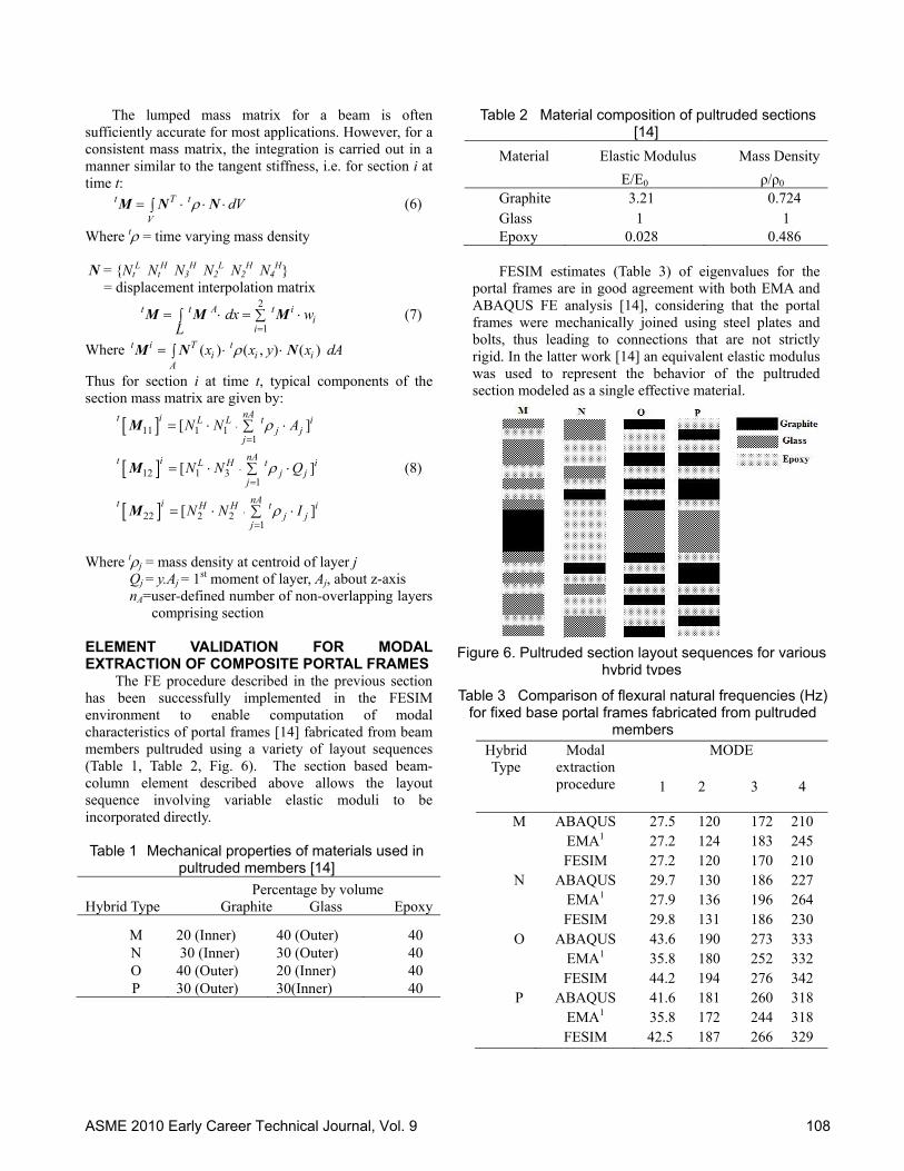
The FE procedure described in the previous section has been successfully implemented in the FESIM environment to enable computation of modal characteristics of portal frames [14] fabricated from beam members pultruded using a variety of layout sequences (Table 1, Table 2, Fig. 6). The section based beam-column element described above allows the layout sequence involving variable elastic moduli to be incorporated directly.

Table 1 Mechanical properties of materials used in

pultruded members [14]

Hybrid Type Percentage by volume

Graphite Glass Epoxy

M 20 (Inner) 40 (Outer) 40 N 30 (Inner) 30 (Outer) 40 O 40 (Outer) 20 (Inner) 40 P 30 (Outer) 30(Inner) 40

Table 2 Material composition of pultruded sections [14]

Material Elastic Modulus Mass Density

E/E0 ρ/ρ0

Graphite 3.21 0.724 Glass 1 1 Epoxy 0.028 0.486

FESIM estimates (Table 3) of eigenvalues for the

portal frames are in good agreement with both EMA and ABAQUS FE analysis [14], considering that the portal frames were mechanically joined using steel plates and bolts, thus leading to connections that are not strictly rigid. In the latter work [14] an equivalent elastic modulus was used to represent the behavior of the pultruded section modeled as a single effective material.

Hybrid Type

Modal extraction procedure

MODE

1

2

3

4

M ABAQUS 27.5 120 172 210 EMA1 27.2 124 183 245 FESIM 27.2 120 170 210

N ABAQUS 29.7 130 186 227 EMA1 27.9 136 196 264 FESIM 29.8 131 186 230

O ABAQUS 43.6 190 273 333 EMA1 35.8 180 252 332 FESIM 44.2 194 276 342

P ABAQUS 41.6 181 260 318 EMA1 35.8 172 244 318 FESIM 42.5 187 266 329

Figure 6. Pultruded section layout sequences for various hybrid types

Table 3 Comparison of flexural natural frequencies (Hz) for fixed base portal frames fabricated from pultruded

members


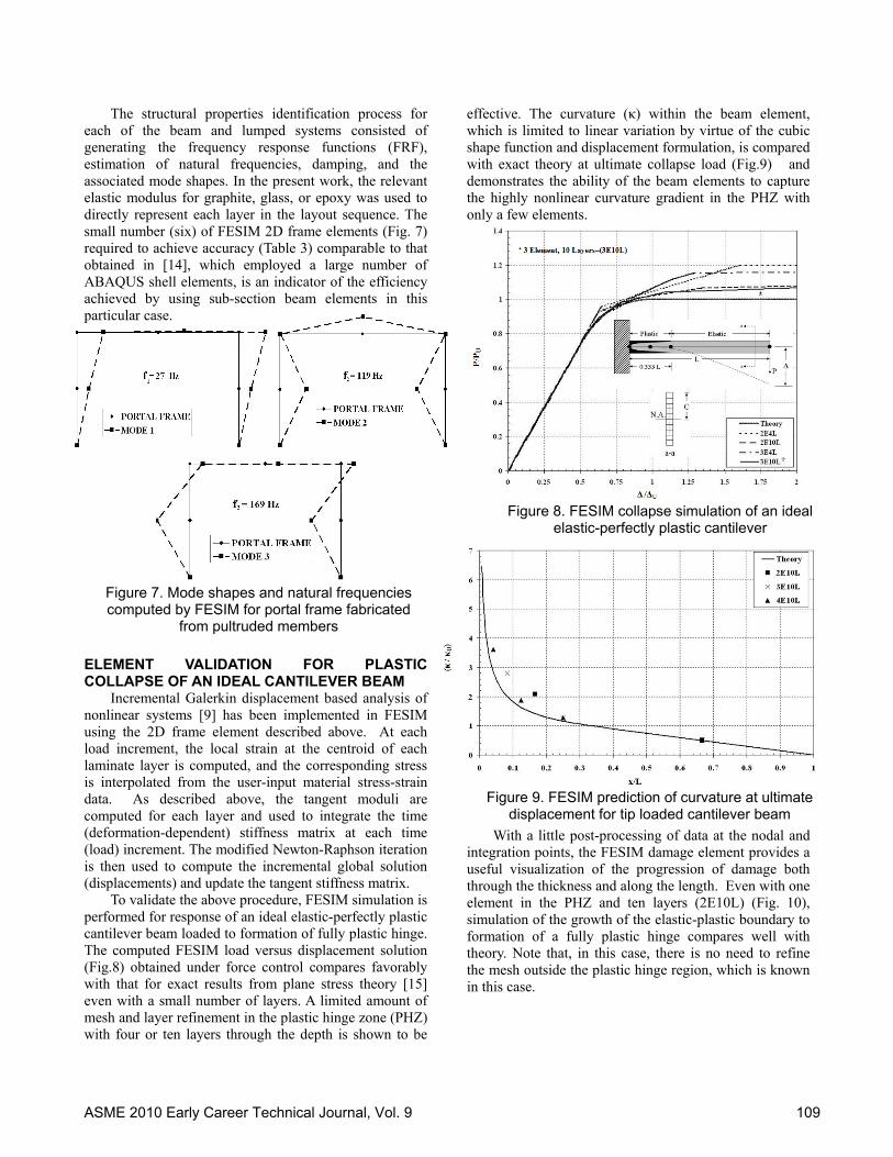
The structural properties identification process for each of the beam and lumped systems consisted of generating the frequency response functions (FRF), estimation of natural frequencies, damping, and the associated mode shapes. In the present work, the relevant elastic modulus for graphite, glass, or epoxy was used to directly represent each layer in the layout sequence. The small number (six) of FESIM 2D frame elements (Fig. 7) required to achieve accuracy (Table 3) comparable to that obtained in [14], which employed a large number of ABAQUS shell elements, is an indicator of the efficiency achieved by using sub-section beam elements in this particular case.

ELEMENT VALIDATION FOR PLASTIC COLLAPSE OF AN IDEAL CANTILEVER BEAM

Incremental Galerkin displacement based analysis of nonlinear systems [9] has been implemented in FESIM using the 2D frame element described above. At each load increment, the local strain at the centroid of each laminate layer is computed, and the corresponding stress is interpolated from the user-input material stress-strain data. As described above, the tangent moduli are computed for each layer and used to integrate the time (deformation-dependent) stiffness matrix at each time (load) increment. The modified Newton-Raphson iteration is then used to compute the incremental global solution (displacements) and update the tangent stiffness matrix.

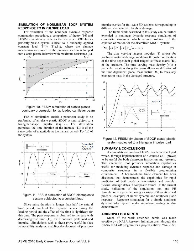
To validate the above procedure, FESIM simulation is performed for response of an ideal elastic-perfectly plastic cantilever beam loaded to formation of fully plastic hinge. The computed FESIM load versus displacement solution (Fig.8) obtained under force control compares favorably with that for exact results from plane stress theory [15] even with a small number of layers. A limited amount of mesh and layer refinement in the plastic hinge zone (PHZ) with four or ten layers through the depth is shown to be

effective. The curvature (κ) within the beam element, which is limited to linear variation by virtue of the cubic shape function and displacement formulation, is compared with exact theory at ultimate collapse load (Fig.9) and demonstrates the ability of the beam elements to capture the highly nonlinear curvature gradient in the PHZ with only a few elements.

With a little post-processing of data at the nodal and

integration points, the FESIM damage element provides a useful visualization of the progression of damage both through the thickness and along the length. Even with one element in the PHZ and ten layers (2E10L) (Fig. 10), simulation of the growth of the elastic-plastic boundary to formation of a fully plastic hinge compares well with theory. Note that, in this case, there is no need to refine the mesh outside the plastic hinge region, which is known in this case.

Figure 8. FESIM collapse simulation of an ideal elastic-perfectly plastic cantilever

Figure 7. Mode shapes and natural frequencies computed by FESIM for portal frame fabricated

from pultruded members

Figure 9. FESIM prediction of curvature at ultimate displacement for tip loaded cantilever beam


SIMULATION OF NONLINEAR SDOF SYSTEM RESPONSE TO IMPULSIVE LOAD For validation of the nonlinear dynamic response computation procedure, a comparison of theory [16] and FESIM simulation is made for the case of a SDOF elastic-perfectly-plastic system subject to a suddenly applied constant load (P(t)) (Fig.11), where the damage mechanism mentioned in the previous section is lumped into elastic-plastic behavior with maximum resistance (R).

FESIM simulations enable a parameter study to be performed of an elasto-plastic SDOF system subject to a triangular-shape impulse (Fig.12). For illustration purposes, the time duration of the impulse (Td) is of the same order of magnitude as the natural period (Tn= T1) of the system.

Since pulse duration is longer than half the natural time period, much of the response occurs during the loading period and the effect of rise time is significant for this case. The peak response is observed to increase with decreasing rise time (Tr), for a constant peak load and impulse. Simulations such as these prove useful in blast vulnerability analyses, enabling development of pressure-

impulse curves for full-scale 3D systems corresponding to different characteristic levels of damage.

The frame work described in this study can be further extended to nonlinear dynamic response simulation of composite structures which require solution of the equation of motion for the discretized MDOF system:

)(tPuuu Gt

Gt

Gt

KCM (9)

The time varying tangent modulus t E allows for nonlinear material damage modeling through modification of the time dependent global tangent stiffness matrix tKG of the structure. The time varying mass density t at a particular location along the beam allows modification of the time dependent global mass matrix tMG to track any changes in mass in the damaged structure.

SUMMARY & CONCLUSIONS

A computational toolbox FESIM has been developed which, through implementation of a concise GUI, proves to be useful for both classroom instruction and research. The interactive tool provides simulation capabilities useful for modeling dynamic response and damage in composite structures in a flexible programming environment. A beam-column finite element has been discussed that demonstrates the capabilities for rapid prediction of both modal characteristics and complex flexural damage states in composite frames. In the current study, validation of the simulation tool and FE formulation are provided using a variety of theoretical and practical examples of linear dynamic and nonlinear static response. Response simulation for a simple nonlinear dynamic sdof system under impulsive loading is also demonstrated.

ACKNOWLEDGEMENTS

Much of the work described herein was made possible by a NASA Research Initiation grant through the NASA EPSCoR program for a project entitled, “An RSST

Figure 12. FESIM simulation of SDOF elasto-plastic system subjected to a triangular impulse load

Figure 11. FESIM simulation of SDOF elastoplastic system subjected to a constant load

Figure 10. FESIM simulation of elastic-plastic boundary progression for tip loaded cantilever beam


for FRP composites airframe substructure design.” The authors also thank Professor Raju Mantena and Dr. Reza Ahmedian for use of experimental and modeling results presented in this paper. NOMENCLATURE B(x): strain-displacement matrix tDNL: time varying nonlinear material matrix tE : time-varying tangent modulus tK: element tangent stiffness matrix (integrated over

volume of element) tKA: tangent stiffness matrix integrated over section

area at numerical integration points (wi) along element length

tM: element consistent mass matrix tMG: global consistent mass matrix NL,x: linear shape function for interpolating axial

displacement NH,xx: cubic Hermitian polynomial shape function for

interpolating flexural displacement td: time varying nodal displacement vector tdA: time varying axial deformation vector at nodes 1

and 2 of element tdB: time varying flexural deformation vector at nodes

1 and 2 of element tε(x): time varying strain-displacement vector at

location x on neutral axis of beam element T0 : natural time period (sec.) T1 : natural time period of 1st mode response (sec.) u1, u2: axial deformation along x-axis at nodes 1 and 2

of element respectively v1, v2: flexural deformation along y-axis at nodes 1 and

2 of element respectively ∆t : time step size θ1, θ2: flexural rotation about z-axis at nodes 1 and 2 of

element respectively t : time varying mass density ζ : damping ratio

REFERENCES [1] The Mathworks, Building GUIs with MATLAB.

Prentice-Hall, 1997 [2] Davalos, J.F., Salim H.A., Qiao, P, Lopez-Anido R.,

Analysis and design of pultruded FRP shapes under bending,. Composites: Part B-Engineering, 27B (1996) 295-305.

[3] Ghiringhelli, G. L., On the linear three-dimensional behavior of composite beams. Composites: Part B-Engineering, 28B (1997) 613-626.

[4] Nori, C. V, McCarty, T. A. and Mantena, P. R., Vibration analysis and finite element modeling for determining shear modulus of pultruded hybrid composites. Composites: Part B-Engineering, 27B (1996) 329-337

[5] Haj-Ali, R. and Kilic H., Nonlinear behavior of pultruded FRP. Composites: Part B-Engineering, 33 (2002) 173-191

[6] Kilic, H. and Haj-Ali, R., Progressive damage and nonlinear analysis of pultruded composite structures. Composites: Part B-Engineering, 34 (2003) 235-250

[7] Ganapathi, M., Flexural loss factors of sandwich and laminated composite beams using linear and nonlinear dynamic analysis. Composites: Part B-Engineering, 30B (1999) 245-256

[8] Chopra, A. K. Dynamics of Structures: Theory and Applications to Earthquake Engineering. 2nd edition. Prentice-Hall, 2001

[9] Bathe, K. J. Finite Element Procedures. Prentice-Hall, 1996

[10] Rao, S. S., Mechanical Vibrations. 3rd edition, Prentice-Hall, 1995

[11] Hibbit, Karlsson & Sorensen, Inc. ABAQUS Users Manual. Version 6.4 .Rhode Island: Providence, 2005

[12] Mullen, C. L. and Cakmak, A. S., A practical 3D column damage element for seismic analysis of RC structures, Computers and Structures, accepted for publication, 2000

[13] Tadepalli, T. P., Interactive computational tools for simulating linear dynamic response and nonlinear quasi-static damage in composite structures. Thesis, Department of Civil Engineering, The University of Mississippi, 2003

[14]Ahmadian, R. and Mantena, P. R., Modal characteristics of structural portal frames made of mechanically joined pultruded flat hybrid composites, Composites: Part B-Engineering, 27B (1996) 319-328

[15] Lubliner, J., Plasticity Theory. Prentice-Hall, 1998 [16] Biggs, J. M., Introduction to Structural Dynamics,

McGraw-Hill Inc., 1964


ASME Early Career Technical Journal

2010 ASME Early Career Technical Conference, ASME ECTC October 1 – 2, Atlanta, Georgia USA

CFD SIMULATION OF THERMAL STRATIFICATION IN PRESSURIZER SURGE LINE

Faisal Asfand Pakistan Nuclear Regulatory Authority

Islamabad, Pakistan

ABSTRACT Thermal stratification is the temperature gradient

along the depth of a fluid. In nuclear power plants the pressurizer surge line is severely affected by thermal stratification. It can cause through-wall cracks, thermal fatigue, unexpected displacement and dislocation of the surge line, and can damage surge line supports. Originally, the thermal stratification load was not considered in nuclear power plants design phase because of the unawareness of the problem. However, analysis shows that the thermal stratification load is significant to affect the structural integrity of the primary circuit in nuclear power plants. For stress analysis of pipes that are subjected to thermal stratification, the temperature profile along the fluid depth must be known. Various CFD (Computational Fluid Dynamics) commercial codes like FLUENT, CFX, Phoenix, etc., can be used to simulate the temperature distribution along the depth of a fluid. In this study simulation of thermal stratification is performed for the pressurizer surge line of the CHASHNUPP Unit-II using CFD code FLUENT 6.1. An unsteady 1st order implicit solver formulation is selected. A standard k-ε model is used for turbulent model, and Boussinesq’s approximation is used for the buoyancy effects. Analysis of the results shows that only a small section of the surge line that is connected to the hot leg is affected by thermal stratification phenomenon to an extent that is negligible. The maximum top-to-bottom temperature observed after running the simulation for 1520 seconds was 27K. The length of the stratified pipe is about 70cm. Analysis confirms that thermal stratification load was included in the design bases. Thermal stratification intensity is not significant to affect the integrity of the pressurizer surge line because the geometry of the pressurizer surge line is in accordance with standards that avoid or minimize thermal stratification. The results of the CFD code are useful to understand the phenomenon and can play an important role in evaluating the structural integrity of the pipe. The results obtained are validated with available literature and are verified with the final safety analysis report of CHASHNUPP Unit-II.

INTRODUCTION A thermally stratified fluid is a fluid that is layered

with different temperatures. A change in temperature leads to a change in the water density. When water flows with a range of temperatures inside a pipe, the lighter, warmer water tends to float on top of the cooler water, resulting in the upper portion of a pipe being hotter than the lower portion. If the water is not sufficiently mixed, the cold and hot portions will separate over the cross-section of the pipe. Under these conditions, differential thermal expansion of the pipe metal can cause the pipe to deflect significantly. Such thermal stratification can play an important role in the aging of nuclear power plant piping because of the stress caused by the temperature difference and the cyclic temperature changes. This stress can limit the lifetime of the piping, even leading to penetrating cracks in areas of high stress concentration or residual stress. Hence, thermal stratification can affect the structural integrity of nuclear power plant pipes.

Stratification is promoted by high temperature differences that increase the difference in density. The development and the stability of the stratified flow depend on the temperature difference and on the relative velocity between the fluids. The typical condition for the occurrence of thermal stratification is when the flow velocities are low and the thermal gradient through the height of the piping system is high. Increasing the flow velocity will enable mixing and remove the stratified state.

Unexpected piping movements are highly undesirable because of the potential for high piping stress that may exceed design limits for fatigue and stress. The problem can become more acute when piping expansion is restricted, such as through contact with pipe whip restraints. Plastic deformation can result and lead to high local stress, low cycle fatigue and functional impairment of the line.

MODEL DESCRIPTION

A pressurizer surge line comes from the hotleg of loop B and is connected to pressurizer at the bottom. The line enables continuous coolant volume pressure


adjustments between the SRC (Reactor Coolant System) and the pressurizer. The pressurizer surge line is made up of “SA 451 CPF8", austenitic stainless steel material. The pressurizer surge line is designed and fabricated to accommodate the system pressures and temperatures attained under all expected modes of plant operation or anticipated system interactions. The design pressure of the pressurizer surge line is 17.2Mpa, and the design temperature is 643K. The surge line’s nominal diameter is 0.273m and its nominal wall thickness is 0.030m. The flow area is 0.036984m2. The length of the pipe is 19.3618m.

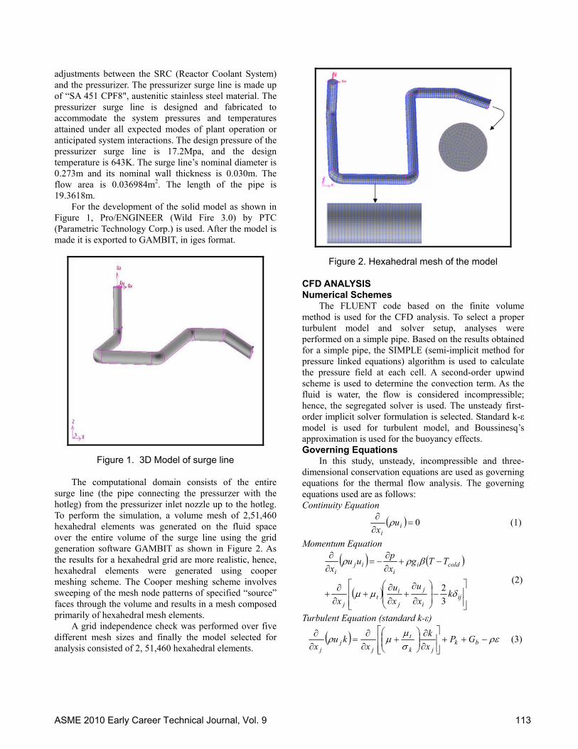
For the development of the solid model as shown in Figure 1, Pro/ENGINEER (Wild Fire 3.0) by PTC (Parametric Technology Corp.) is used. After the model is made it is exported to GAMBIT, in iges format.

Figure 1. 3D Model of surge line

The computational domain consists of the entire surge line (the pipe connecting the pressurzer with the hotleg) from the pressurizer inlet nozzle up to the hotleg. To perform the simulation, a volume mesh of 2,51,460 hexahedral elements was generated on the fluid space over the entire volume of the surge line using the grid generation software GAMBIT as shown in Figure 2. As the results for a hexahedral grid are more realistic, hence, hexahedral elements were generated using cooper meshing scheme. The Cooper meshing scheme involves sweeping of the mesh node patterns of specified “source” faces through the volume and results in a mesh composed primarily of hexahedral mesh elements.

A grid independence check was performed over five different mesh sizes and finally the model selected for analysis consisted of 2, 51,460 hexahedral elements.

Figure 2. Hexahedral mesh of the model

CFD ANALYSIS Numerical Schemes

The FLUENT code based on the finite volume method is used for the CFD analysis. To select a proper turbulent model and solver setup, analyses were performed on a simple pipe. Based on the results obtained for a simple pipe, the SIMPLE (semi-implicit method for pressure linked equations) algorithm is used to calculate the pressure field at each cell. A second-order upwind scheme is used to determine the convection term. As the fluid is water, the flow is considered incompressible; hence, the segregated solver is used. The unsteady first-order implicit solver formulation is selected. Standard k-ε model is used for turbulent model, and Boussinesq’s approximation is used for the buoyancy effects. Governing Equations

In this study, unsteady, incompressible and three-dimensional conservation equations are used as governing equations for the thermal flow analysis. The governing equations used are as follows: Continuity Equation

0

ii

ux

(1)

Momentum Equation

iji

j

j

it

j

coldii

iji

kx

u

x

u

x

TTgx

puu

x

3

2 (2)

Turbulent Equation (standard k-ε)

bkjk

t

jj

j

GPx

k

xku

x (3)


21 CGPCk

xxu

x

bk

j

t

jj

j

(4)

Energy Equation

jp

f

t

t

jj

j x

T

C

k

xTu

x

(5)

Where, the coefficient, source term, and turbulent constants are as follows:

Cµ = 0.09, C1 = 1.44, C2 = 1.92

/2kCt

j

i

i

j

j

itk x

u

x

u

x

uP

ii

t

tb x

TgG

After the setup of the solver (FLUENT), the solution

was initialized (provide initial guesses to start iterations). As thermal stratification is a transient phenomenon, unsteady analyses were performed. These unsteady analyses were performed using a time step of 1 second, and 100 iterations per time step. The convergence criterion is that the residual is less than 1x10-4 for the continuity equation and less than 1x10-5 for others at each time step. To satisfy this convergence criterion, iterations of less than 100 per time step of 1 second are needed. An unsteady CFD simulation was performed for 1520 seconds. To improve the convergence, under-relaxation factors were applied. Boundary Conditions

The end of the pressurizer surge line that is attached to the pressurizer is set for velocity inlet while the end that is attached to the hot leg is set for pressure outlet. The coolant with higher temperature (617K) enters from the pressurizer into the surge line with a velocity of 0.02 m/s. In the main loop, coolant with lower temperature (585K) flows. For the outlet boundary condition, 0Pa relative pressure was set. To obtain a clear pattern of stratification, the variable density parameter is selected. Density is calculated and stated at each temperature point between 585K and 617K using the piecewise-linear parameter in the solver.

RESULTS AND DISCUSSIONS Thermal Flow Analysis

To evaluate the temperature distributions for the pressurizer surge line, a transient three-dimensional numerical thermal hydraulic analysis was performed using the CFD code FLUENT 6.1.

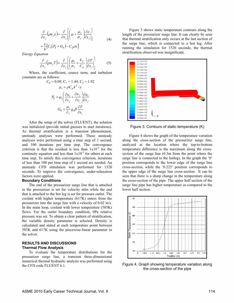
Figure 3 shows static temperature contours along the length of the pressurizer surge line. It can clearly be seen that thermal stratification only occurs at the last section of the surge line, which is connected to a hot leg. After running the simulation for 1520 seconds, the thermal stratification observed was insignificant.

Figure 3. Contours of static temperature (K) Figure 4 shows the graph of the temperature variation

along the cross-section of the pressurizer surge line, analyzed at the location where the top-to-bottom temperature difference is the maximum along the cross-section of the surge line (0.3m from the point where the surge line is connected to the hotleg). In the graph the ‘0’ position corresponds to the lower edge of the surge line cross-section, while the ‘0.225’ position corresponds to the upper edge of the surge line cross-section. It can be seen that there is a sharp change in the temperature along the cross-section of the pipe. The upper half section of the surge line pipe has higher temperature as compared to the lower half section.

Figure 4. Graph showing temperature variation along the cross-section of the pipe


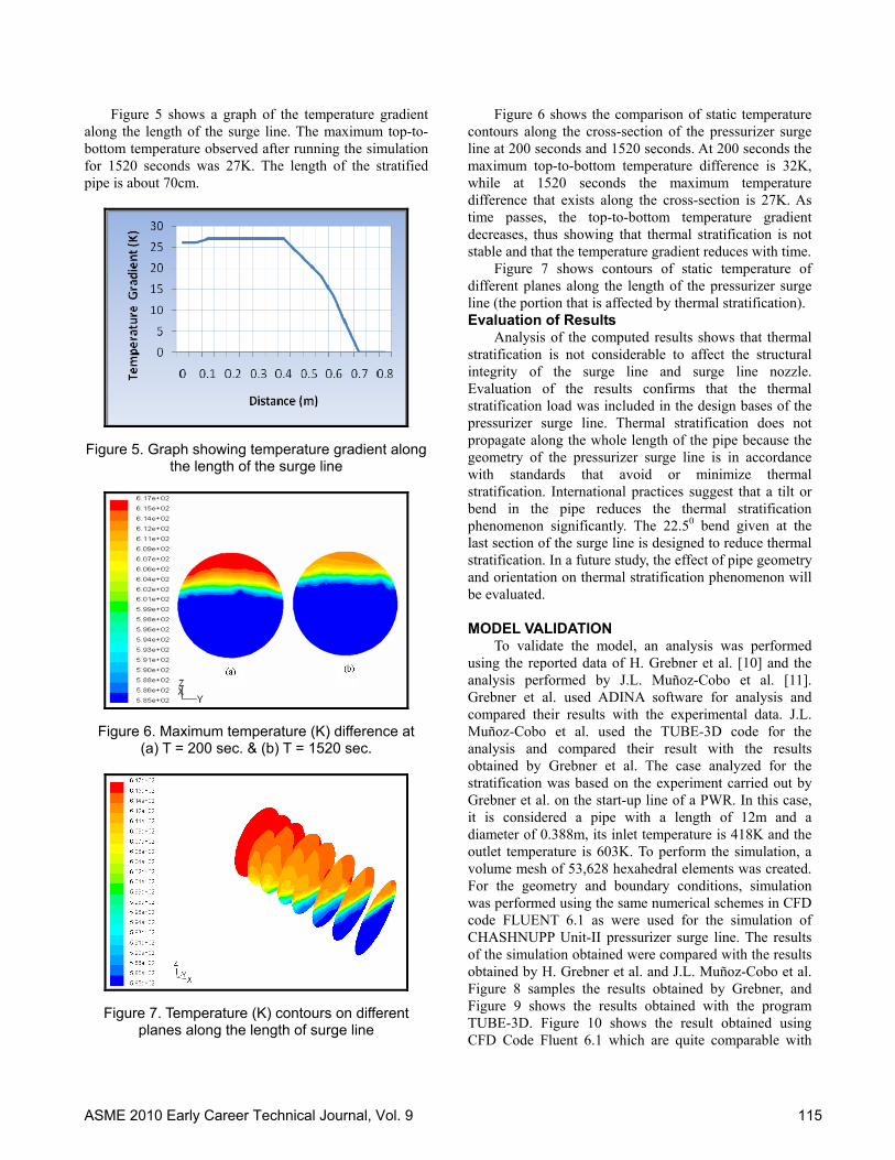
Figure 5 shows a graph of the temperature gradient along the length of the surge line. The maximum top-to-bottom temperature observed after running the simulation for 1520 seconds was 27K. The length of the stratified pipe is about 70cm.

Figure 5. Graph showing temperature gradient along the length of the surge line

Figure 6. Maximum temperature (K) difference at (a) T = 200 sec. & (b) T = 1520 sec.

Figure 7. Temperature (K) contours on different planes along the length of surge line

Figure 6 shows the comparison of static temperature contours along the cross-section of the pressurizer surge line at 200 seconds and 1520 seconds. At 200 seconds the maximum top-to-bottom temperature difference is 32K, while at 1520 seconds the maximum temperature difference that exists along the cross-section is 27K. As time passes, the top-to-bottom temperature gradient decreases, thus showing that thermal stratification is not stable and that the temperature gradient reduces with time.

Figure 7 shows contours of static temperature of different planes along the length of the pressurizer surge line (the portion that is affected by thermal stratification). Evaluation of Results

Analysis of the computed results shows that thermal stratification is not considerable to affect the structural integrity of the surge line and surge line nozzle. Evaluation of the results confirms that the thermal stratification load was included in the design bases of the pressurizer surge line. Thermal stratification does not propagate along the whole length of the pipe because the geometry of the pressurizer surge line is in accordance with standards that avoid or minimize thermal stratification. International practices suggest that a tilt or bend in the pipe reduces the thermal stratification phenomenon significantly. The 22.50 bend given at the last section of the surge line is designed to reduce thermal stratification. In a future study, the effect of pipe geometry and orientation on thermal stratification phenomenon will be evaluated.

MODEL VALIDATION

To validate the model, an analysis was performed using the reported data of H. Grebner et al. [10] and the analysis performed by J.L. Muñoz-Cobo et al. [11]. Grebner et al. used ADINA software for analysis and compared their results with the experimental data. J.L. Muñoz-Cobo et al. used the TUBE-3D code for the analysis and compared their result with the results obtained by Grebner et al. The case analyzed for the stratification was based on the experiment carried out by Grebner et al. on the start-up line of a PWR. In this case, it is considered a pipe with a length of 12m and a diameter of 0.388m, its inlet temperature is 418K and the outlet temperature is 603K. To perform the simulation, a volume mesh of 53,628 hexahedral elements was created. For the geometry and boundary conditions, simulation was performed using the same numerical schemes in CFD code FLUENT 6.1 as were used for the simulation of CHASHNUPP Unit-II pressurizer surge line. The results of the simulation obtained were compared with the results obtained by H. Grebner et al. and J.L. Muñoz-Cobo et al. Figure 8 samples the results obtained by Grebner, and Figure 9 shows the results obtained with the program TUBE-3D. Figure 10 shows the result obtained using CFD Code Fluent 6.1 which are quite comparable with


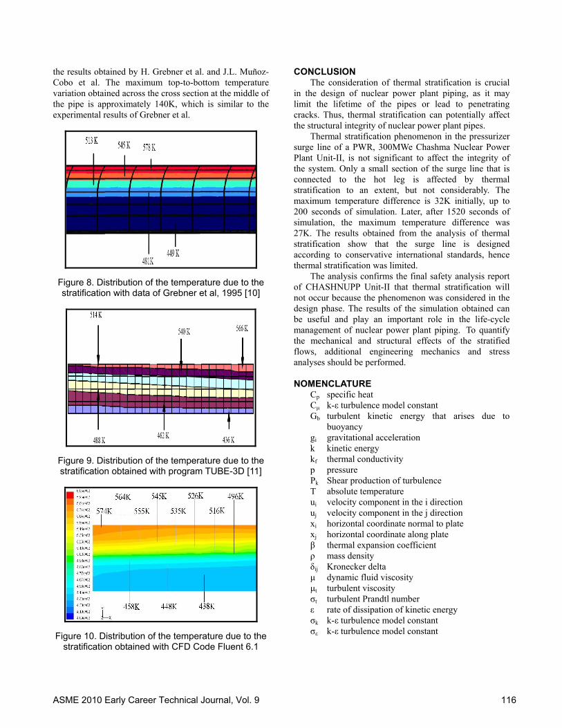
the results obtained by H. Grebner et al. and J.L. Muñoz-Cobo et al. The maximum top-to-bottom temperature variation obtained across the cross section at the middle of the pipe is approximately 140K, which is similar to the experimental results of Grebner et al.

Figure 8. Distribution of the temperature due to the stratification with data of Grebner et al, 1995 [10]

Figure 9. Distribution of the temperature due to the stratification obtained with program TUBE-3D [11]

Figure 10. Distribution of the temperature due to the stratification obtained with CFD Code Fluent 6.1

CONCLUSION The consideration of thermal stratification is crucial

in the design of nuclear power plant piping, as it may limit the lifetime of the pipes or lead to penetrating cracks. Thus, thermal stratification can potentially affect the structural integrity of nuclear power plant pipes.

Thermal stratification phenomenon in the pressurizer surge line of a PWR, 300MWe Chashma Nuclear Power Plant Unit-II, is not significant to affect the integrity of the system. Only a small section of the surge line that is connected to the hot leg is affected by thermal stratification to an extent, but not considerably. The maximum temperature difference is 32K initially, up to 200 seconds of simulation. Later, after 1520 seconds of simulation, the maximum temperature difference was 27K. The results obtained from the analysis of thermal stratification show that the surge line is designed according to conservative international standards, hence thermal stratification was limited.

The analysis confirms the final safety analysis report of CHASHNUPP Unit-II that thermal stratification will not occur because the phenomenon was considered in the design phase. The results of the simulation obtained can be useful and play an important role in the life-cycle management of nuclear power plant piping. To quantify the mechanical and structural effects of the stratified flows, additional engineering mechanics and stress analyses should be performed.

NOMENCLATURE

Cp specific heat Cμ k-ε turbulence model constant Gb turbulent kinetic energy that arises due to

buoyancy gi gravitational acceleration k kinetic energy kf thermal conductivity p pressure Pk Shear production of turbulence T absolute temperature ui velocity component in the i direction uj velocity component in the j direction xi horizontal coordinate normal to plate xj horizontal coordinate along plate β thermal expansion coefficient ρ mass density δij Kronecker delta μ dynamic fluid viscosity μt turbulent viscosity σt turbulent Prandtl number ε rate of dissipation of kinetic energy σk k-ε turbulence model constant σε k-ε turbulence model constant


ACKNOWLEDGMENTS The author highly acknowledges Mr. Jamil Ahmed

Meenai and Dr. Syed Anwar ul Hasson for their guidance and valuable information through out this research work.

REFERENCES [1] Dahlberg, M., et al., “Development of a European Procedure for Assessment of High Cycle Thermal Fatigue in Light Water Reactors”, Final Report of the NESC Thermal Fatigue Project, 2007. [2] FLUENT User’s Guide, Fluent Inc., (1998). [3] GAMBIT 2.3 Documentation, Fluent Inc., (1998). [4] Kim, K. C., Lim, J. H., and Yoon, J. K., “Thermal Fatigue estimation due to thermal stratification in the RCS branch line using one-way FSI scheme”, Journal of Mechanical Science and Technology, 22, pp 2218-2227, 2008. [5] JHUNG, M. J., and CHOI, Y. H., “Surge Line Stress Due To Thermal Stratification”, Nuclear Engineering and Technology, 40, 2008. [6] Boros, I., and Aszódi, A., “Analysis of thermal stratification in the primary circuit of a VVER-440 reactor with the CFX code”, Nuclear Engineering and Design, 238, pp. 453-459, 2008. [7] Kim, Y. J., Kim M. W., Ko, E., Lee, J. G., and Kim, B. C., 2009, “Effect of Heat-Up Transient Condition on the Thermal Stratification in Nuclear Power Plant Surgeline”,

Proc. Pressure Vessels and Piping Conference, Prague, Czech Republic, 4, pp. 99-104. [8] Kang D. G., and Jo, J. C., “3-D Transient CFD Analysis for the Structural Integrity Assessment of a PWR Pressurizer Surge Line Subjected to Thermally Stratified Flow”, Safety Issue Research Department, Korea Institute of Nuclear Safety, Korea, 2007. [9] Kim, S. N., Hwang, S. H., and Yoon, K. H., “Experiments on the Thermal Stratification in the Branch of NPP”, Journal of Mechanical Science and Technology, 19, pp. 1206-1215, 2005. [10] Grebner, H., Höfler, A., “Investigation of Stratification Effects on the Surge Line of a Pressurised Water Reactor”, Computers and Structures, 56, pp. 425- 437, 1995. [11] Muñoz-Cobo, J. L., Escrivá, A., and Rosa, J. C., “Liquid Temperature Stratification in Piping of Nuclear Power Plants”, Universidad Politécnica de Valencia, Spain. [12] USNRC, “Pressurizer Surge Line Thermal Stratification”, Bulletin No. 88-11, Washington, D.C. 20555, 1988. [13] EPRI, “Thermal Stratification”, Cycling and Striping (TASCS), TR-103581, 1994. [14] Patankar, S. V., 1980, “Numerical Heat Transfer and Fluid Flow”, McGraw-Hill Book Company.



October 1-2, 2010, Atlanta, Georgia, USA

FLOWCHART VISUAL PROGRAMMING IN MECHATRONICS COURSE

Vidya K. Nandikolla Philadelphia University Philadelphia, PA, USA

Suhas S. Pharkute PCS Edventures, Inc.

Boise, ID, USA

ABSTRACT Mechatronics systems represent a multidisciplinary approach to system design. Since it is the integration of mechanical engineering with electronics and intelligent computer control, teaching this course to non-computer science engineering students can be challenging. Mechanical Engineering (ME) students, before enrolling into “Introduction to Mechatronics” course, pass “Intro to Computing” and “Electrical Engineering Fundamentals” courses, but fail to engage and become motivated to develop competence. The study focuses on discussing a methodology of integrating programming concepts using a flow chart system with designing, building and simulating electromechanical systems. In this paper, a learning style for mechanical engineering undergraduate students building a visual process to understand the bridging of the hardware and software in mechatronics systems is implemented. The paper describes a teaching method of how to program a robot by developing an easy understanding pattern for writing logic for C programming language. Initially, students learn how to integrate the mechanical, electrical, electronic systems together, followed by understanding of the microcontroller interface. This proposed method helps students to minimize syntax related problems and to improve in their algorithm development challenges. INTRODUCTION

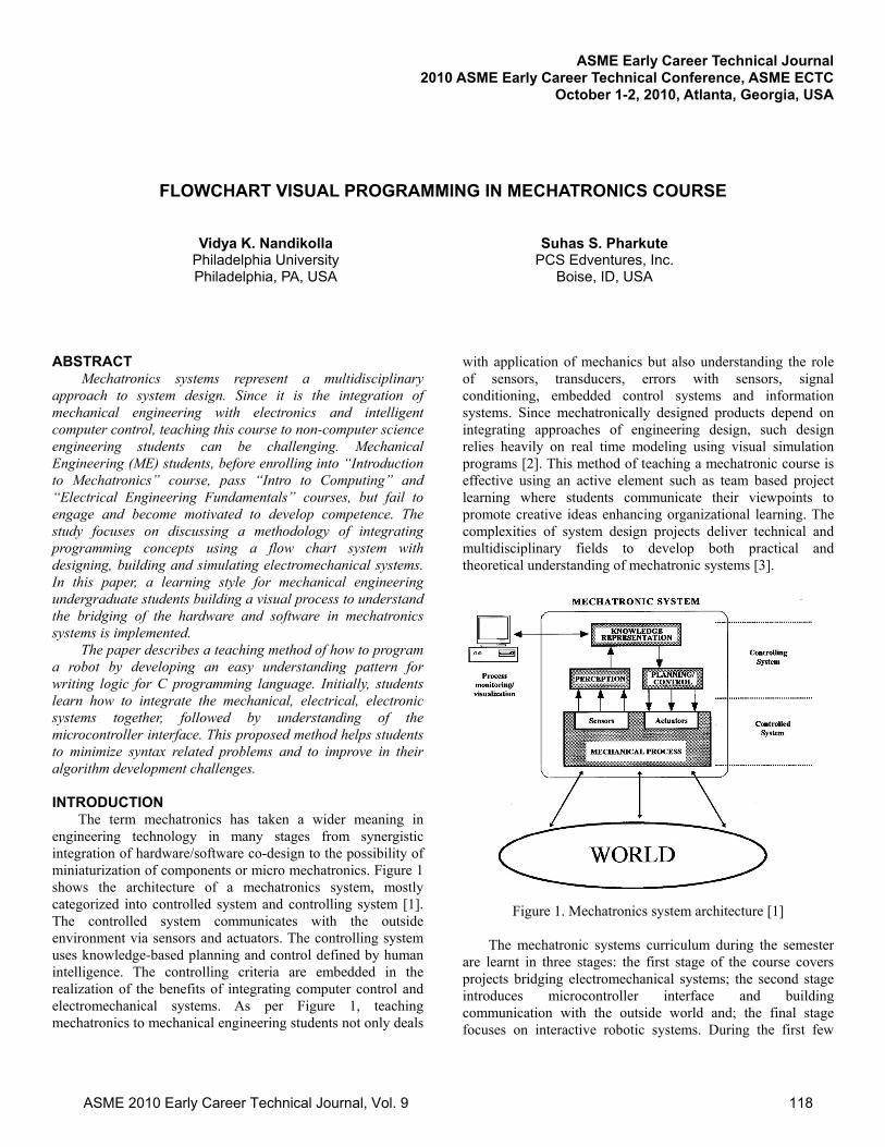
The term mechatronics has taken a wider meaning in engineering technology in many stages from synergistic integration of hardware/software co-design to the possibility of miniaturization of components or micro mechatronics. Figure 1 shows the architecture of a mechatronics system, mostly categorized into controlled system and controlling system [1]. The controlled system communicates with the outside environment via sensors and actuators. The controlling system uses knowledge-based planning and control defined by human intelligence. The controlling criteria are embedded in the realization of the benefits of integrating computer control and electromechanical systems. As per Figure 1, teaching mechatronics to mechanical engineering students not only deals

with application of mechanics but also understanding the role of sensors, transducers, errors with sensors, signal conditioning, embedded control systems and information systems. Since mechatronically designed products depend on integrating approaches of engineering design, such design relies heavily on real time modeling using visual simulation programs [2]. This method of teaching a mechatronic course is effective using an active element such as team based project learning where students communicate their viewpoints to promote creative ideas enhancing organizational learning. The complexities of system design projects deliver technical and multidisciplinary fields to develop both practical and theoretical understanding of mechatronic systems [3].

Figure 1. Mechatronics system architecture [1]

The mechatronic systems curriculum during the semester

are learnt in three stages: the first stage of the course covers projects bridging electromechanical systems; the second stage introduces microcontroller interface and building communication with the outside world and; the final stage focuses on interactive robotic systems. During the first few


weeks of the course, students implement the fundamentals of basic mechanics, synthesis of mechanism, kinematic analysis, gears and gear trains, electrical circuits, integrated circuits, different sensors, motors, H-bridge, and signal processing. The later half of the curriculum introduces prototyping circuit boards, microcontroller programming, sensor calibration, motor speed control, energy transfer mechanism and towards the end students build a robotic vehicle for final competition.

Computer programming plays an important role in mechatronics design from modeling, simulation, validation, visualization, data collection, data processing to digital control [4, 5]. Though computer programming is a fundamental aspect for most engineering courses, teaching and learning in traditional methods does not necessarily show the implementation. In the “Introduction to Computing” course, typically students learn a specific programming language but struggle to see how it can be used outside of PC environment or how is it relevant to mechanical engineering [6].

In this paper, we are discussing a method of using a flowchart system to generate the logic and translate to a visual program and later write the equivalent C code. Now the question arises: “why not the usual traditional lecture style?” There can be many responses, but we see the majority of students struggle to learn a simple method to program, and they end up making it more complicated and confusing than required. Here we are attempting to change the perception of programming for undergraduate mechanical engineering students to make them comfortable with software coding since everything today is automated. The following sections will give details of the development of the method but first we will discuss the importance of Project Based Learning (PBL) since our motto is based on teams working together in projects.

WHY PROJECT BASED LEARNING?

Learning styles vary among individual students; however, psychological research shows that humans remember only 10% of the content that they read and 90% of what they experience. It is well known that students learn better and become engaged if the contents are taught by seeing and doing compared to only hearing [3, 7]. Research in engineering education demonstrates its ineffectiveness in lecture-based delivery of materials. Concern about the ineffectiveness has been raised by professional and educators, but still remains dominated by the "chalk and talk" technique [8]. To overcome these concerns, PBL enables students to understand the synthesis of interdisciplinary engineering fields to culminate a powerful, adaptable method of learning that models industrial practice. Team project based learning with open-ended problems better prepares engineering graduates for challenges in real-world engineering jobs including increasing communication skills, writing skills, presentation and project management skills [9, 10]. With team involvement, students contribute towards the learning of others, improve constructive cognitive activity and promote learning.

ROBOTICS PROJECT In this section, we discuss a simple robotic project from an

Introduction to Mechatronics course followed by a teaching method to help students understand how to logically process the information of a required assignment. We mainly focus on the computing control part of the project rather than the mechanical structure of the robot. During the initial weeks of the course, the teams work together to design and build their robot integrating sensors, actuators, microcontroller communications and other components. Generally, students enjoy the hands-on experience building an electromechanical system and their designs are creative. In the typical process behind the scene, right after students have their robots ready, they jump directly to programming without much planning. If they are not able to calibrate the sensors or communicate with the motors, they end up with frustration, discouragement and quickly blame the programming course or how poorly they got to see the integration to the real world.

In this paper, we are trying to train students how to begin the logical thinking for programming before actually beginning to write the code. The first task for the students is to write the logical steps of the problem, then understand the fundamentals of their program like loops, conditional execution, compilers, in system program and lastly read the sensor outputs and translate to the microcontroller language. In the process of discussing and determining the structured approach, the teams make sure the functions of the robot are programmed dynamically so when the tasks are changed, they don’t have to modify the complete program, instead it is automated. In the following section the flow chart visual learning concept demonstrates the proposed method for teaching programming to ME students in mechatronics course.

FLOW CHART VISUAL LEARNING

Programming is understood as planning and writing the process of a proposed solution to a problem using some computer language. The syntax development is not difficult but keep in mind the computer does not think, it only follows the instructions expressed. Since the computer programming only processes the instructions, the teams cover all possibilities of occurrence. After the set of tasks are assigned to the students, they first determine the flow process for their program logic that includes reading of sensor values, calibrating, defining various cases of occurrences and its conditions. The students also incorporate error-checking method and determine the optimal coding flow for their program. Once they have finalized the method, they draw a flow chart of the process and later translate it into a visual program and C code. Once C code is generated they download the program to the brain (microcontroller board) of the robot and start the testing process. Our main focus is the flow chart development process, which offers students problem solving analysis and exposes them to the basic tenets of algorithm thinking [6].

In building the flow chart based programming, the students understand the strategy of algorithm development better. The


reason why we choose robotic systems is: (a) to demonstrate to ME students how software controls the mechanical systems simulating an industrial scenario, and (b) because the students are fascinated with mobile robots, which injects the fun element and teaches them the principles of programming, a win-win situation. METHODOLOGY

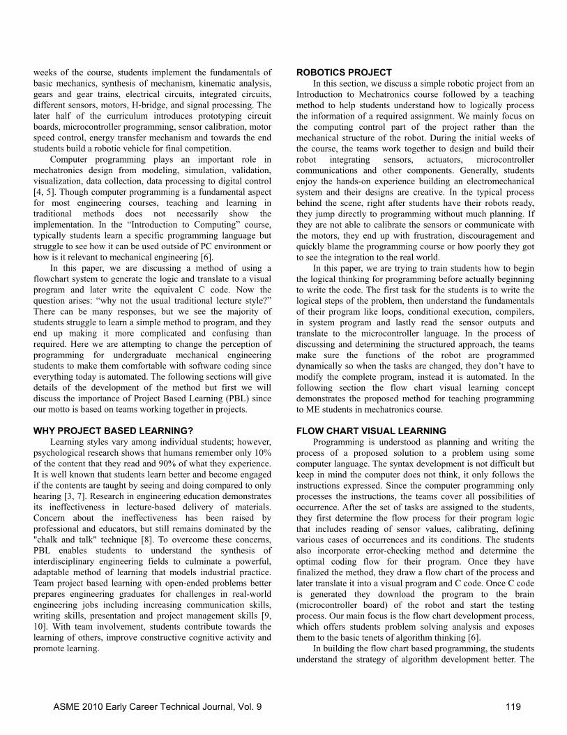
For the robot following a zigzag black line, students first determine their logical steps: the number of sensors they need, the physical distance between the sensors, the turning direction of the robot, motor drive control, motor on and off. First they develop simple functions, which are dynamic in nature for turn right, left, and move forward. Then, they develop their logic: calibrating sensor readings, identifying the black and white colors and determining the threshold value to control the path of the robot. The robot not traveling in a straight line would be an error, so they program it accurately for the robot to travel straight. The teams use two IR sensors and two motors, and determine four cases of possibility and fine-tuning. Figure 2 shows a flow chart for a line following robot, a simple exercise to learn how to use conditional statements. Here are the details of the flow chart from Figure 2:

The first assumption considered is, by turning motors in clockwise direction the vehicle moves in a forward direction. Process:

1. At the start, the vehicle moves in forward direction 2. Read Left and Right Sensors (LS and RS) and there

can be only following 4 cases a. LS < 500 AND RS > 500: This means LS is reading

black and RS is reading white color, indicating that vehicle is too far on right side and needs to turn to the left

b. LS > 500 AND RS < 500: This is exactly opposite of case ‘a’ where RS is reading black and LS is reading white color, indicating that vehicle is too far left and needs to turn to the right

c. LS > 500 AND RS > 500: This case means the black line is between 2 sensors so vehicle needs to move straight forward, and no turns

d. LS < 500 AND RS < 500: This case is near impossible to happen unless the black area covers both sensors at the same time, in this case, it is optimal to stop

The details of dynamic functions for move forward, left and right turnings (Figure 3): To ‘Move Forward’ function:

Turn on both motors in clockwise direction To ‘Turn Left’ function:

Turn on left motor in counterclockwise direction and right motor in clockwise direction

Wait for 1 sec Turn on both motors in clockwise direction

To ‘Turn Right’ function: Turn on right motor in counterclockwise direction and

left motor in clockwise direction Wait for 1 sec Turn on both motors in clockwise direction

To calibrate the sensors:

Take a reading from sensor on black surface (B) Take a reading from sensor on white surface (W) Find mean ( (B + W)/2 ) and that is the threshold

value. In our case it is 500

Figure 2: Flow chart for black line follower

The flow process described in Figure 2 is ready to be

developed using a PCS cortex visualization program which uses a drag and drop technique (Figure 4). The students use this program initially to understand the structure of loops and conditions and how they branch out from the flow process. This software easily converts the grahical interface to simple C code which is very helpful for some students with not much coding experience. Eventually, the ME students after gaining


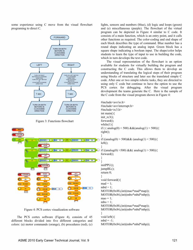
some experience using C move from the visual flowchart programing to direct C.

Figure 3: Functions flowchart

Figure 4: PCS cortex visualization software

The PCS cortex software (Figure 4), consists of 45

different blocks divided into five different categories and colors: (a) motor commands (orange), (b) procedures (red), (c)

lights, sensors and numbers (blue), (d) logic and loops (green) and (e) miscellaneous (purple). The flowchart of the virtual program can be depicted in Figure 4 similar to C code. It consists of a main function, which is an entry point, and it calls other functions as required. The color-coding and end shape of each block describes the type of command. Blue number has a round shape indicating an analog input. Green block has a square shape indicating a boolean input. The shape/color helps students to learn the type of input to use in building the code, which in turn develops the text code.

The visual representation of the flowchart is an option avaliable for students for virtually building the program and constructing the C code. This allows them to develop an understanding of translating the logical steps of their program using blocks of structure and later see the translated simple C code. After one or two simple robotic tasks, they are directed to using only C code but continue to have the option to use the PCS cortex for debugging. After the visual program development the teams generate the C. Here is the sample of the C code from the visual program shown in Figure 4:

#include<avr/io.h> #include<avr/interrupt.h> #include<rc3.h> int main(){ init_rc3(); forward(); while(1){ if ( ( analog(0) < 500) &&(analog(1) > 500)){ right(); } if ((analog(0) > 500)&& (analog(1) < 500)){ left(); } if ((analog(0) >500) &&( analog(1) > 500)){ forward(); } } initPPU(); jumpBL(); return 0; } void forward(){ mad = 1; mbd = 1; MOTOR(0x88,(int)(mao*mad*map)); MOTOR(0x84,(int)(mbo*mbd*mbp)); mao = 1; mbo = 1; MOTOR(0x88,(int)(mao*mad*map)); MOTOR(0x84,(int)(mbo*mbd*mbp)); } void left(){ mbd = -1; MOTOR(0x84,(int)(mbo*mbd*mbp));


mbo = 1; MOTOR(0x84,(int)(mbo*mbd*mbp)); delay_hms( 10 ); mbo = 0; MOTOR(0x84,(int)(mbo*mbd*mbp)); mbd = 1; MOTOR(0x84,(int)(mbo*mbd*mbp)); mbo = 1; MOTOR(0x84,(int)(mbo*mbd*mbp)); } void right(){ mad = -1; MOTOR(0x88,(int)(mao*mad*map)); mao = 1; MOTOR(0x88,(int)(mao*mad*map)); delay_hms( 10 ); mao = 0; MOTOR(0x88,(int)(mao*mad*map)); mad = 1; MOTOR(0x88,(int)(mao*mad*map)); mao = 1; MOTOR(0x88,(int)(mao*mad*map)); } The C code is downloaded/tested and fine-tuned to make sure the robot functions as per their design. The errors are adjusted and the fun begins of racing among groups. Figure 5 shows a mechanical robot following the line.

Figure 5: Line following robot

The aim of introducing this method of programming was to allow ME students to familiarize with the concepts of developing a structured programming art. Prior to this course the students already learn flow chart as a planning tool, here we used the flow chart method to show the relationship between the software planning and programming using graphical representation [11, 12].

DISCUSSION

These days we are getting creative to deliver engineering education to better prepare our future graduates with hands-on

experience and innovative thinking. In this paper we are presenting a method implemented in an Introduction to Mechatronics course in our ME curriculum showing the importance of algorithm development similar to real world industrial practices. A quantitative measurement was implemented in the classroom for improving the learning methods of the students. Using this style of visualization, students found useful implementing their instructional materials learnt in their computing course and implementing in more application-oriented class. The aim of the project was to introduce programming via a flowchart mechanism, with group discussions, teamwork and competitive environment among students. The response from students showed change in their perception in programming. The improvement in their coding is noticeable towards the end of the semester compared to the start. The simple method of teaching showed significant number of mechanical engineering students the relevance of programming in their study, especially in robotics. The students were motivated, enthusiastic and wanted more challenges in their curriculum. The overall impact sounded promising, although low percentage of students still have difficulty with the flowchart method and C coding but gained better understanding of logical thinking. It is clear that active learning is useful in today’s study process and needs continuous improvement.

REFERENCES [1] Popovchenko, M., 2006, “Introduction to Mechatronics and Mechatronics in Real Life,” Mechatronics Foundations and Applications, http://www14.informatik.tu-muenchen.de/konferenzen/Jass06/courses/5/index.html#popovchenko [2] Shetty, D., Kondo, J., Campana, C., and Kolk, R. A., 2002, “Real-Time Mechatronic Design Process for Research and Education,” ASEE Annual Conference & Exposition Proceedings, Montrel, Quebec. [3] Wen-Jye, S., 2010, “Teaching Mechatronics: An Innovative Group Project-Based Approach,” Computer Application in Engineering Education, Wiley Periodicals Inc. [4] Chen, X.Q., Gaynor, P., King, R., Chase, J.G., Bones, P., Gough, P., and Duke, R., 2008, “A Project-Based Mechatronics Program to Reinforce Mechatronic Thinking – A Restructuring Experience from University of Canterbury,” http://ir.canterbury.ac.nz/handle/10092/2208 [5] Craig, K., 2003, “Role of Computers in Mechatronics,” IEEE Computer in Science and Engineering, 5, pp. 80-85. [6] Bateson, A. D., Brown, N. J., and Wilkinson, A. J., 2010, “Flowchart Driven Robot to Promote Educational Development (FRED),” Engineering Education 2010 Inspiring the next generation of engineers, p38, http://www.ee2010.info/programme-papers.asp [7] Reisman, S., and Carr, W. A., 1991, “Perspectives on Multimedia Systems in Education,” IBM Systems Journal, 30, pp. 280-295.


[8] Mills, J., 2002, “A Case Study of Project-Based Learning in Structural Engineering”, ASEE Annual Conference and Exposition, Montrel, Quebec. [9] Price, A., Rimington, R., Chew, M.T., and Demidenko, S., 2010, “Project-Based Learning in Robotics and Electronics in Undergraduate Engineering Program Setting,” 5th IEEE International Symposium on Electronic Design, Test and Applications, pp.188-193. [10] Nandikolla, V., Shadle, S., Gardner, J., Grover, R., and Pharkute, S., 2008, “Real World Industry Collaboration within a Mechatronics Class”, Frontiers in Education (FIE), 38th Annual Conference. [11] Carlisle, M. C., Wilson, T. A., Humphries, J. W., and Hadfield, S. M., 2004, “Raptor: Introducing Programming to Non-Majors with Flowcharts,” Journal of Computing in Small Colleges, 19, pp. 52-60. [12] Crews, T. and Zieger, U., 1998, “The Flowchart Interpreter for Introductory Programming Courses,” Proceedings of FIE Conference, pp. 307-312.



October 1 – 2, Atlanta, Georgia USA

ADAPTIVE MULTI AIRBAG SHOE INSERT FOR DIABETIC FOOT CARE

Vidya K. Nandikolla, Jenna Matthews Philadelphia University Philadelphia, PA, USA

Marco P. Schoen Idaho State University

Pocatello, ID, USA

Suhas S. Pharkute Syna Intelligence Boise, ID, USA

Uwe Reischl Boise State University

Boise, ID, USA

Ajay Mahajan The University of Akron

Akron, OH, USA

ABSTRACT Diabetic mellitus patients have foot problems such as loss of sensation, insufficient blood flow to lower extremities and alterations in shape of their pressure patterns causing concentrated high pressure regions. These peaks are due to the disfunctional feed back system from their mechanoreceptors and may lead to complex problems such as amputation if not identified and treated in timely manner. Our main objective is to protect the foot by sensing the abnormal peaks and redistribute the pressure from excessive pressure regions. Therefore, we are developing a design layout for an adaptable shoe insert useful for diabetic foot care. In this paper, the design of adaptive footwear using multi airbag measurement system is presented as a part of our design phase I. The human foot anatomy and anthropometry is studied and insole footwear is designed to auto sense the pressure distribution of the diabetic foot. The biomechanical foot design using a spring-mass-damper mathematical model is used to analyze the mechanical energy distribution and the patterns of stress and strain affecting the foot. The proposed multi airbag shoe insert has a sensing grid that measures the actual pressure of the diabetic patient. The optimal pressure distribution pattern is calculated using foot and insert models and the contact foot pressures are adjusted accordingly reducing the error between the normal and abnormal distribution. The pressure control unit adjusts the airbag shoe insert controlled by the dynamical system. The proposed adaptive multi airbag shoe insert design prototype can be very useful for diabetic foot care. INTRODUCTION

One of the major complications associated with diabetics is neuropathy, mainly caused due to partial or complete loss of sensation in the feet. It leads to problems like inadequate delivery of nutrients and oxygen to the foot causing healing impairment. The common symptoms diagnosed with neuropathy are pain and numbness in the legs or feet. The numbness tends to result into blisters and sores and areas of

unnatural pressure peaks. Due to the loss of sensory feedback system in diabetic patients they are not able to adjust their stance, and expose their feet to high peaks for a long time causing complexity with the foot pressure distribution. Many researchers suggest that it is possible to avoid foot problems caused due to the elevated pressure peaks by identifying and taking appropriate measures like smart in-shoe footwear [1, 2].

The recent treatments to plantar pressures are custom made shoe inserts, prescription running shoes, rocker bottom shoes, super depth shoes with soft insoles and molded insoles or soft plugs [3-5]. Most therapeutic footwear is effective to relieve high pressures at focal area under the foot as long as the placement are well understood which can be challenging. These materials allow compression of the footwear in the areas of high pressure peaks but may generate stress at the edges. There are studies available in therapeutic footwear in terms of design, selection of suitable shoe insert for a patient with high risk of ulceration that are based on experience and intuition of the physician rather than scientific principles. Finite element modeling is used extensively to investigate foot models for therapeutic footwear design but generalization is not easy since there can be many design variables for wide range of patient characteristics [6].

Foot pressure reduction and redistribution can be achieved by fabricating orthotic devices based on foot structure, and analyzing external loads and tissue mechanics. The common cause of the diabetic planter ulcers is excessive foot pressures in localized regions of the foot. Research shows 75% of the foot ulcers occur beneath the metatarsal heads due to painless and unnoticed trauma occurring during regular activities [7]. Other conditions such as abnormal biomechanical factors or excess foot pronation also influence loading on plantar fascia, which causes pain and inflammation [8] that can be treated using conservative therapy. The human foot is subject to substantial forces during day-to-day activities. If we consider the foot like any structure designed with a set of linkages having rigid or flexible joints and ligaments at each joint, then upon loading the deformation is restricted to maintain the


integrity of the longitudinal arch of the foot [8]. This means the foot is capable of storing strain energy and returning to elastic region. The footwear described in [7] using patient specific finite element model can be effective in reducing peak plantar pressure under the metatarsal head. In another research study [9], human heel pad is considered to transient the forces at the heel strike region since it is the major source of energy absorption. Reviewing the research focused in different types of foot models and footwear, we are integrating a design of multi airbag shoe insert which autosenses and redistributes the pressure peaks.

In our proposed research work we are investigating and designing a prototype, which will study the plantar pressure distribution of forces in the foot and is capable of executing the measurement and control tasks as directed. The foot pressure distribution for a diabetic patient mostly has different patterns compared to a healthy subject due to stress levels associated with neuropathy. A simple comparison between the two can reveal the high pressure points, which produces ulcers creating complexity in the disorder. Sensing the irregular pressure distribution and redistribution is the objective of the proposed design of the prototype. FOOT STRUCTURE

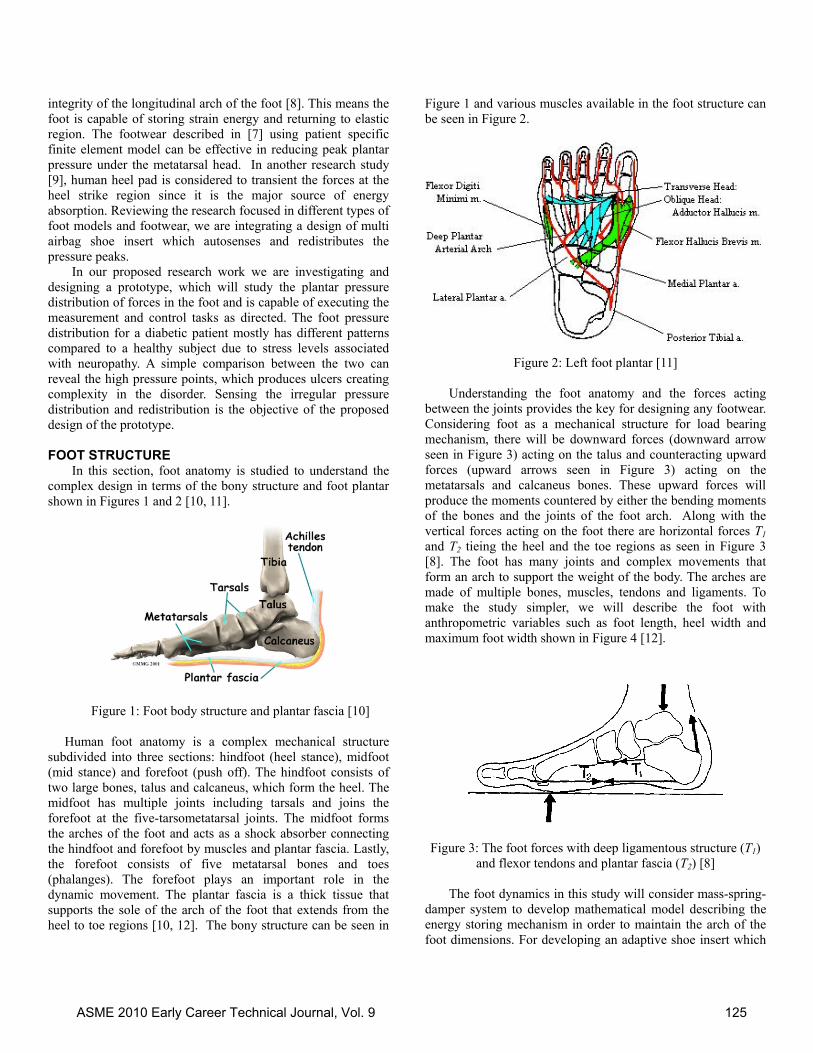
In this section, foot anatomy is studied to understand the complex design in terms of the bony structure and foot plantar shown in Figures 1 and 2 [10, 11].

Figure 1: Foot body structure and plantar fascia [10] Human foot anatomy is a complex mechanical structure subdivided into three sections: hindfoot (heel stance), midfoot (mid stance) and forefoot (push off). The hindfoot consists of two large bones, talus and calcaneus, which form the heel. The midfoot has multiple joints including tarsals and joins the forefoot at the five-tarsometatarsal joints. The midfoot forms the arches of the foot and acts as a shock absorber connecting the hindfoot and forefoot by muscles and plantar fascia. Lastly, the forefoot consists of five metatarsal bones and toes (phalanges). The forefoot plays an important role in the dynamic movement. The plantar fascia is a thick tissue that supports the sole of the arch of the foot that extends from the heel to toe regions [10, 12]. The bony structure can be seen in

Figure 1 and various muscles available in the foot structure can be seen in Figure 2.

Figure 2: Left foot plantar [11]

Understanding the foot anatomy and the forces acting

between the joints provides the key for designing any footwear. Considering foot as a mechanical structure for load bearing mechanism, there will be downward forces (downward arrow seen in Figure 3) acting on the talus and counteracting upward forces (upward arrows seen in Figure 3) acting on the metatarsals and calcaneus bones. These upward forces will produce the moments countered by either the bending moments of the bones and the joints of the foot arch. Along with the vertical forces acting on the foot there are horizontal forces T1 and T2 tieing the heel and the toe regions as seen in Figure 3 [8]. The foot has many joints and complex movements that form an arch to support the weight of the body. The arches are made of multiple bones, muscles, tendons and ligaments. To make the study simpler, we will describe the foot with anthropometric variables such as foot length, heel width and maximum foot width shown in Figure 4 [12].

Figure 3: The foot forces with deep ligamentous structure (T1) and flexor tendons and plantar fascia (T2) [8]

The foot dynamics in this study will consider mass-spring-

damper system to develop mathematical model describing the energy storing mechanism in order to maintain the arch of the foot dimensions. For developing an adaptive shoe insert which


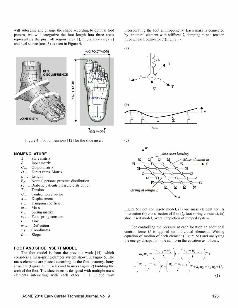
will autosense and change the shape according to optimal foot pattern, we will categorize the foot length into three areas representing the push off region (area 1), mid stance (area 2) and heel stance (area 3) as seen in Figure 4.

Figure 4: Foot dimensions [12] for the shoe insert

NOMENCLATURE A … State matrix B… Input matrix C… Output matrix D … Direct trans. Matrix L … Length

Pde… Normal persons pressure distribution Pex … Diabetic patients pressure distribution

T … Tension U … Control force vector d … Displacement c … Damping coefficient m … Mass k … Spring matrix kp … Foot spring constant t … Time w … Deflection x,y … Coordinates … Slope

FOOT AND SHOE INSERT MODEL The foot model is from the previous work [14], which

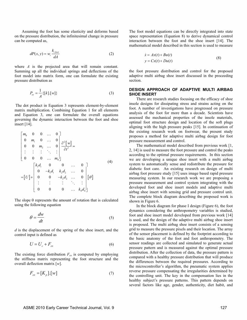
considers a mass-spring-damper system shown in Figure 5. The mass elements are placed according to the foot anatomy, bony structure (Figure 1), muscles and tissues (Figure 2) building the arch of the foot. The shoe insert is designed with multiple mass elements interacting with each other in a unique way

incorporating the foot anthropometry. Each mass is connected by structural element with stiffness k, damping c, and tension through each connector T (Figure 5). (a)

(b)

(c)

Figure 5: Foot and insole model, (a) one mass element and its interaction (b) cross section of foot (kp foot spring constant), (c) shoe insert model, overall depiction of lumped system.

For controlling the pressure at each location an additional control force U is applied on individual elements. Writing equation of motion of each element (Figure 5a) and analyzing the energy dissipation, one can form the equation as follows.

, 1 1, 1i i ii ii i iii ii

w w w wm w T T

L L

.

1, 1 , , 1, 1i i i i i i i iii ii ii ii ii

w w w wT T k w c w U

L L

(1)


Assuming the foot has some elasticity and deforms based on the pressure distribution, the infinitesimal change in pressure can be computed as,

( , ) i footi

kdP x y w

dA (2)

where A is the projected area that will remain constant. Summing up all the individual springs and deflections of the foot model into matrix form, one can formulate the existing pressure distribution as

1

{[ ].[ ]}exP k wA

(3)

The dot product in Equation 3 represents element-by-element matrix multiplication. Combining Equation 1 for all elements and Equation 3, one can formulate the overall equations governing the dynamic interaction between the foot and shoe insert [14].

0

1 2

2 2

4

1 1

1 1 2 2

2 2

4 4

0 0 0

0 0 0

0 0 0

0 0 0

0 0 0

0 0

0 0 0

0 0 0

m

mw

mt

m

k d

k d k d

U k d

k d

(4)

The slope represents the amount of rotation that is calculated using the following equation

dw

dt (5)

d is the displacement of the spring of the shoe insert, and the control input is defined as U Uc Fex (6) The existing force distribution Fex is computed by employing the stiffness matrix representing the foot structure and the overall deflection matrix [w]. Fex [K p ].[w] (7)

The foot model equations can be directly integrated into state space representation (Equation 8) to derive dynamical control interaction between the foot and the shoe insert [14]. The mathematical model described in this section is used to measure

( ) ( )

( ) ( )

x Ax t Bu t

y Cx t Du t

(8)

the foot pressure distribution and control for the proposed adaptive multi airbag shoe insert discussed in the proceeding section.

DESIGN APPROACH OF ADAPTIVE MULTI AIRBAG SHOE INSERT

There are research studies focusing on the efficacy of shoe insole designs for dissipating stress and strains acting on the foot. A number of investigations have progressed on pressure analysis of the foot for more than a decade. Scientists have assessed the mechanical properties of the insole materials, optimal foot structure design and location of the soft plugs aligning with the high pressure peaks [15]. In continuation of the existing research work on footwear, the present study proposes a method for adaptive multi airbag design for foot pressure measurement and control.

The mathematical model described from previous work [1, 2, 14] is used to measure the foot pressure and control the peaks according to the optimal pressure requirements. In this section we are developing a unique shoe insert with a multi airbag system to automatically sense and redistribute the pressure for diabetic foot care. An existing research on design of multi airbag foot pressure study [15] uses image based rapid pressure measuring system. In our research work we are proposing a pressure measurement and control system integrating with the developed foot and shoe insert models and adaptive multi airbag shoe insert with sensing grid and pressure control unit. The complete block diagram describing the proposed work is shown in Figure 6.

In the block diagram for phase I design (Figure 6), the foot dynamics considering the anthropometry variables is studied, foot and shoe insert model developed from previous work [14] is used, and the design of the adaptive multi airbag shoe insert is proposed. The multi airbag shoe insert consists of a sensing grid to measure the pressure pixels and their location. The array of the sensor placement is defined by the footprint according to the basic anatomy of the foot and foot anthropometry. The sensor readings are collected and simulated to generate actual pressure pattern and is measured against the optimal pressure distribution. After the collection of data, the pressure pattern is compared with a healthy pressure distribution that will produce the differences between the required pressures. According to the microcontroller’s algorithm, the pneumatic system applies reverse pressure compensating the irregularities determined by the controlling unit. The key in the compensation lies in the healthy subject’s pressure patterns. This pattern depends on several factors like age, gender, authenticity, diet habit, and


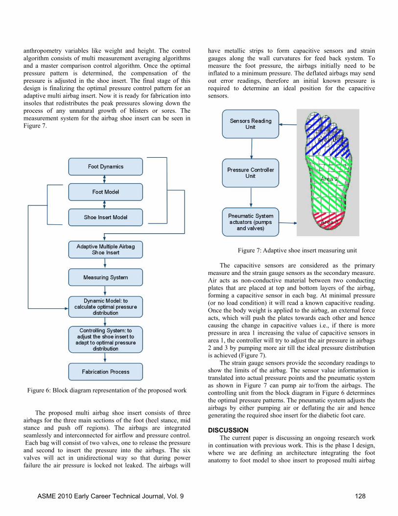
anthropometry variables like weight and height. The control algorithm consists of multi measurement averaging algorithms and a master comparison control algorithm. Once the optimal pressure pattern is determined, the compensation of the pressure is adjusted in the shoe insert. The final stage of this design is finalizing the optimal pressure control pattern for an adaptive multi airbag insert. Now it is ready for fabrication into insoles that redistributes the peak pressures slowing down the process of any unnatural growth of blisters or sores. The measurement system for the airbag shoe insert can be seen in Figure 7.

Figure 6: Block diagram representation of the proposed work

The proposed multi airbag shoe insert consists of three

airbags for the three main sections of the foot (heel stance, mid stance and push off regions). The airbags are integrated seamlessly and interconnected for airflow and pressure control. Each bag will consist of two valves, one to release the pressure and second to insert the pressure into the airbags. The six valves will act in unidirectional way so that during power failure the air pressure is locked not leaked. The airbags will

have metallic strips to form capacitive sensors and strain gauges along the wall curvatures for feed back system. To measure the foot pressure, the airbags initially need to be inflated to a minimum pressure. The deflated airbags may send out error readings, therefore an initial known pressure is required to determine an ideal position for the capacitive sensors.

Figure 7: Adaptive shoe insert measuring unit

The capacitive sensors are considered as the primary measure and the strain gauge sensors as the secondary measure. Air acts as non-conductive material between two conducting plates that are placed at top and bottom layers of the airbag, forming a capacitive sensor in each bag. At minimal pressure (or no load condition) it will read a known capacitive reading. Once the body weight is applied to the airbag, an external force acts, which will push the plates towards each other and hence causing the change in capacitive values i.e., if there is more pressure in area 1 increasing the value of capacitive sensors in area 1, the controller will try to adjust the air pressure in airbags 2 and 3 by pumping more air till the ideal pressure distribution is achieved (Figure 7).

The strain gauge sensors provide the secondary readings to show the limits of the airbag. The sensor value information is translated into actual pressure points and the pneumatic system as shown in Figure 7 can pump air to/from the airbags. The controlling unit from the block diagram in Figure 6 determines the optimal pressure patterns. The pneumatic system adjusts the airbags by either pumping air or deflating the air and hence generating the required shoe insert for the diabetic foot care.

DISCUSSION

The current paper is discussing an ongoing research work in continuation with previous work. This is the phase I design, where we are defining an architecture integrating the foot anatomy to foot model to shoe insert to proposed multi airbag


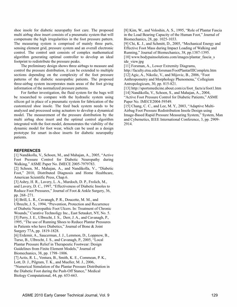
shoe insole for diabetic neuropathy foot care. The proposed multi airbag shoe insert consists of a pneumatic system that will compensate the high irregularities in the foot pressure pattern. The measuring system is comprised of mainly three parts, sensing element grid, pressure system and an overall electronic control. The control unit consists of complex mathematical algorithm generating optimal controller to develop an ideal footprint to redistribute the pressure peaks.

The preliminary design shows three airbags to measure and control the pressure distribution, it can be extended to multiple sections depending on the complexity of the foot pressure patterns of the diabetic neuropathic patients. The proposed three-airbag system incorporates main areas of the foot giving information of the normalized pressure patterns.

For further investigation, the fluid system for the bags will be researched to compare with the hydraulic system using silicon gel in place of a pneumatic system for fabrication of the customized shoe insole. The feed back system needs to be analyzed and processed using actuators to develop a dynamical model. The measurement of the pressure distribution by the multi airbag shoe insert and the optimal control algorithm integrated with the foot model, demonstrates the viability of the dynamic model for foot wear, which can be used as a design prototype for smart in-shoe inserts for diabetic neuropathy patients.

REFERENCES [1] Nandikolla, V., Schoen, M., and Mahajan, A., 2005, “Active Foot Pressure Control for Diabetic Neuropathy during Walking,” ASME Paper No. IMECE 2005-7979783. [2] Schoen, M., Mahajan, A., and Nandikolla, V., “Diabetic Foot,” 2010, Distributed Diagnosis and Home Healthcare, American Scientific Press, Chap.6. [3] Ashry, H. R., Lavery, L. A., Murdoch, D. P., Frolich, M., and Lavery, D. C., 1997, “Effectiveness of Diabetic Insoles to Reduce Foot Pressures,” Journal of Foot & Ankle Surgery, 36, pp. 268–271. [4] Brill, L. R., Cavanagh, P. R., Doucette, M. M., and Ulbrecht, J. S., 1994, “Prevention, Protection and Recurrence of Diabetic Neuropathic Foot Ulcers. In: Treatment of Chronic Wounds,” Curative Technoligy Inc., East Setauket, NY, No. 5. [5] Perry, J. E., Ulbrecht, J. S., Derr, J. A., and Cavanagh, P., 1995, “The use of Running Shoes to Reduce Plantar Pressures in Patients who have Diabetics,” Journal of Bone & Joint Surgery 77A, pp. 1819-1828. [6] Erdemir, A., Saucerman, J. J., Lemmon, D., Loppnow, B., Turso, B., Ulbrecht, J. S., and Cavanagh, P., 2005, “Local Plantar Pressure Relief in Therapeutic Footwear: Design Guidelines from Finite Element Models,” Journal of Biomechanics, 38, pp. 1798–1806. [7] Actis, R. L., Ventura, B., Smith, K. E., Commean, P. K., Lott, D. J., Pilgram, T. K., and Mueller, M. J., 2006, “Numerical Simulation of the Plantar Pressure Distribution in the Diabetic Foot during the Push-Off Stance,” Medical Biology Computational, 44, pp. 653-663.

[8] Kim, W., and Voloshin, A. S., 1995, “Role of Plantar Fascia in the Load Bearing Capacity of the Human Foot,” Journal of Biomechanics, 28, pp. 1025-1033. [9] Chi, K. J., and Schmitt, D., 2005, “Mechanical Energy and Effective Foot Mass during Impact Loading of Walking and Running,” Journal of Biomechanics, 38, pp.1387-1395. [10] www.bodypainsolutions.com/images/plantar_fascia_s ide_view.jpg [11] Forsman, A., Lower Extremity Diagrams, http://faculty.etsu.edu/forsman/FootPlantarIIIComplete.htm [12] Agic, A., Nikolic, V., and Mijovic, B., 2006, “Foot Anthropometry and Morphology Phenomena,” Collegium Antropologicum, 30, pp. 815-821. [13] http://sportsmedicine.about.com/cs/foot_facts/a/foot1.htm [14] Nandikolla, V., Schoen, S., and Mahajan, A., 2004, “Active Foot Pressure Control for Diabetic Patients,” ASME Paper No. IMECE2004-59549. [15] Chang, C. C., and Lee, M. Y., 2003, “Adaptive Multi-Airbag Foot Pressure Redistribution Insole Design using Image-Based Rapid Pressure Measuring System,” System, Man and Cybernetics, IEEE International Conference, 3, pp. 2909-2914.



2010 ASME Early Career Technical Conference, ASME ECTC October 1-2, 2010, Atlanta, Georgia, USA

DESIGN APPROACH TO FIRE LIFE SAFETY IN TUNNELS THROUGH THE USE OF SUBWAY ENVIRONMENT SIMULATION SOFTWARE

Bradley L. Zundel AECOM

Oakland, California, USA

ABSTRACT Fire life safety is an essential aspect in the design of transit

and roadway tunnels. Complexities of tunnel fires include increased temperature at the fire thereby increasing the rate at which it grows, potential for collapse due to concrete spalling, entrapment of patrons, lack of visibility, restricted access for fire personnel, and the entrapment of noxious fumes. Therefore, it is imperative to provide operational protective systems within a network of tunnels, as in a subway system, to ensure all safety needs are addressed.

With regard to tunnel fire safety, there are two general design strategies: prescriptive-based design and performance-based design. Performance-based design pertains to engineering analysis which predicts the effects of a fire. This level of design is applied to active fire protection systems which include ventilation systems and water-based suppression systems

Modeling a tunnel network with an active ventilation system can be analyzed through subway environment simulation (SES) software. The input to the program and the output produced by the program are tailored for design engineers concerned with practical environmental problems. The software consists of five subprograms: Train performance; Aerodynamic; Thermodynamic, consisting of Temperature/humidity and Heat sink/environmental control; and Fire effects. The following will introduce how SES computer software has elevated the success of optimizing the environment within a tunnel network. INTRODUCTION

Fire life safety is an essential aspect in the design of transit and roadway tunnels. As long as sources of combustion exist in tunnels there is an ever-present danger of igniting a fire by which life, property, and economic vitality is threatened. Even though there was no loss of life, the Channel Tunnel fire in 1996 resulted in one half of the tunnel being out of service for 6 months [1] at a cost of £200 million; this does not factor in the cost to industry and to the British economy as a whole [2]. Therefore, transit system authorities require strict design criteria to limit the catastrophic effects of a fire.

The reason tunnel fires are so burdensome is due to the fire being in an enclosed space. This brings about a number of difficulties, including: increased temperature at the fire thereby increasing the rate at which it grows [3], potential for collapse due to concrete spalling, entrapment of patrons, lack of visibility, restricted access for fire personnel, and the entrapment of noxious fumes. Therefore, it is imperative to provide operational protective systems within a network of tunnels, as in a subway system, to ensure all safety needs are addressed. Fire safety of systems is achieved through a composite of facility design, operating equipment, hardware, procedures, and software subsystems that are integrated to provide requirements for the protection of life and property from the effects of fire [4]. METHODS OF DESIGN

With regard to tunnel fire safety, there are two general design strategies. The first is prescriptive-based design standards and regulations. These include best practice codes and guides; for instance, the spacing between fire extinguishers within a road tunnel [5]. The second is performance-based design. This includes engineering analysis to predict the effects of a fire. The majority of this paper will deal with performance-based design, specifically through the use of computer modeling. FIRE PROTECTION SYSTEMS

Passive as well as active fire protection systems are essential deterrents as part of an overall environmental control through aerodynamic and thermodynamic principles. Passive protection systems include (1) a secondary layer of a concrete applied to the inner surface of a tunnel, (2) panels made of protective material fixed to tunnel walls and ceilings, or (3) certain fibers mixed in with the main concrete to render the concrete more fire resistant [1]. Active fire protection systems include ventilation systems and water-based suppression systems with the main goal of providing an adequate tenable environment during evacuation. Common practices include both passive and active fire protection systems to be in use.


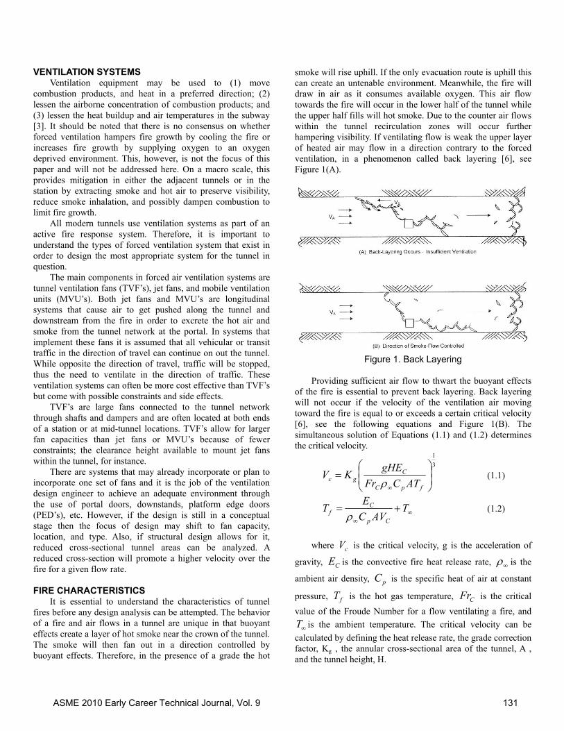
VENTILATION SYSTEMS Ventilation equipment may be used to (1) move

combustion products, and heat in a preferred direction; (2) lessen the airborne concentration of combustion products; and (3) lessen the heat buildup and air temperatures in the subway [3]. It should be noted that there is no consensus on whether forced ventilation hampers fire growth by cooling the fire or increases fire growth by supplying oxygen to an oxygen deprived environment. This, however, is not the focus of this paper and will not be addressed here. On a macro scale, this provides mitigation in either the adjacent tunnels or in the station by extracting smoke and hot air to preserve visibility, reduce smoke inhalation, and possibly dampen combustion to limit fire growth.

All modern tunnels use ventilation systems as part of an active fire response system. Therefore, it is important to understand the types of forced ventilation system that exist in order to design the most appropriate system for the tunnel in question.

The main components in forced air ventilation systems are tunnel ventilation fans (TVF’s), jet fans, and mobile ventilation units (MVU’s). Both jet fans and MVU’s are longitudinal systems that cause air to get pushed along the tunnel and downstream from the fire in order to excrete the hot air and smoke from the tunnel network at the portal. In systems that implement these fans it is assumed that all vehicular or transit traffic in the direction of travel can continue on out the tunnel. While opposite the direction of travel, traffic will be stopped, thus the need to ventilate in the direction of traffic. These ventilation systems can often be more cost effective than TVF’s but come with possible constraints and side effects.

TVF’s are large fans connected to the tunnel network through shafts and dampers and are often located at both ends of a station or at mid-tunnel locations. TVF’s allow for larger fan capacities than jet fans or MVU’s because of fewer constraints; the clearance height available to mount jet fans within the tunnel, for instance.

There are systems that may already incorporate or plan to incorporate one set of fans and it is the job of the ventilation design engineer to achieve an adequate environment through the use of portal doors, downstands, platform edge doors (PED’s), etc. However, if the design is still in a conceptual stage then the focus of design may shift to fan capacity, location, and type. Also, if structural design allows for it, reduced cross-sectional tunnel areas can be analyzed. A reduced cross-section will promote a higher velocity over the fire for a given flow rate. FIRE CHARACTERISTICS

It is essential to understand the characteristics of tunnel fires before any design analysis can be attempted. The behavior of a fire and air flows in a tunnel are unique in that buoyant effects create a layer of hot smoke near the crown of the tunnel. The smoke will then fan out in a direction controlled by buoyant effects. Therefore, in the presence of a grade the hot

smoke will rise uphill. If the only evacuation route is uphill this can create an untenable environment. Meanwhile, the fire will draw in air as it consumes available oxygen. This air flow towards the fire will occur in the lower half of the tunnel while the upper half fills will hot smoke. Due to the counter air flows within the tunnel recirculation zones will occur further hampering visibility. If ventilating flow is weak the upper layer of heated air may flow in a direction contrary to the forced ventilation, in a phenomenon called back layering [6], see Figure 1(A).

Figure 1. Back Layering

Providing sufficient air flow to thwart the buoyant effects

of the fire is essential to prevent back layering. Back layering will not occur if the velocity of the ventilation air moving toward the fire is equal to or exceeds a certain critical velocity [6], see the following equations and Figure 1(B). The simultaneous solution of Equations (1.1) and (1.2) determines the critical velocity.

31

⎟⎟⎠

⎞⎜⎜⎝

⎛=

∞ fpC

Cgc ATCFr

gHEKVρ

(1.1)

∞∞

+= TAVC

ETCp

Cf ρ

(1.2)

where cV is the critical velocity, g is the acceleration of

gravity, CE is the convective fire heat release rate, ∞ρ is the

ambient air density, pC is the specific heat of air at constant

pressure, fT is the hot gas temperature, CFr is the critical

value of the Froude Number for a flow ventilating a fire, and

∞T is the ambient temperature. The critical velocity can be calculated by defining the heat release rate, the grade correction factor, Kg , the annular cross-sectional area of the tunnel, A , and the tunnel height, H.


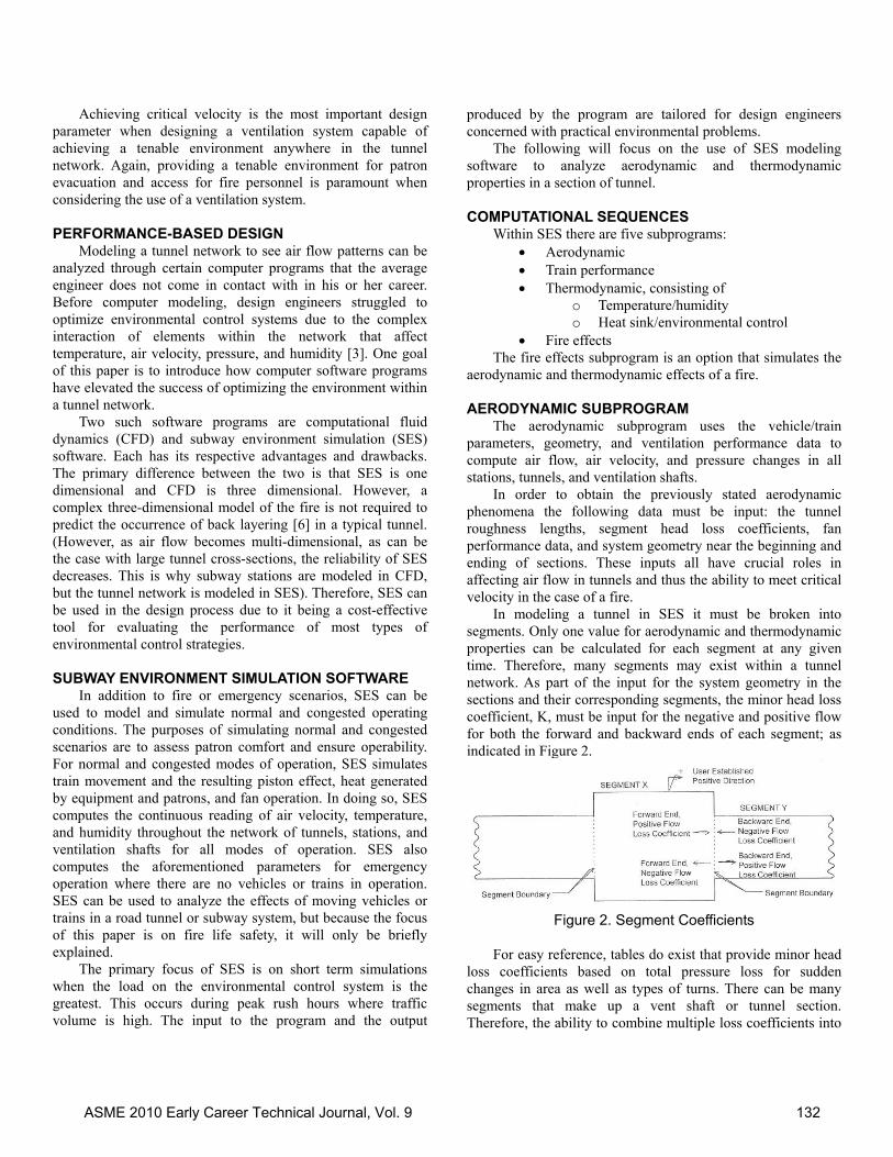
Achieving critical velocity is the most important design parameter when designing a ventilation system capable of achieving a tenable environment anywhere in the tunnel network. Again, providing a tenable environment for patron evacuation and access for fire personnel is paramount when considering the use of a ventilation system. PERFORMANCE-BASED DESIGN

Modeling a tunnel network to see air flow patterns can be analyzed through certain computer programs that the average engineer does not come in contact with in his or her career. Before computer modeling, design engineers struggled to optimize environmental control systems due to the complex interaction of elements within the network that affect temperature, air velocity, pressure, and humidity [3]. One goal of this paper is to introduce how computer software programs have elevated the success of optimizing the environment within a tunnel network.

Two such software programs are computational fluid dynamics (CFD) and subway environment simulation (SES) software. Each has its respective advantages and drawbacks. The primary difference between the two is that SES is one dimensional and CFD is three dimensional. However, a complex three-dimensional model of the fire is not required to predict the occurrence of back layering [6] in a typical tunnel. (However, as air flow becomes multi-dimensional, as can be the case with large tunnel cross-sections, the reliability of SES decreases. This is why subway stations are modeled in CFD, but the tunnel network is modeled in SES). Therefore, SES can be used in the design process due to it being a cost-effective tool for evaluating the performance of most types of environmental control strategies. SUBWAY ENVIRONMENT SIMULATION SOFTWARE

In addition to fire or emergency scenarios, SES can be used to model and simulate normal and congested operating conditions. The purposes of simulating normal and congested scenarios are to assess patron comfort and ensure operability. For normal and congested modes of operation, SES simulates train movement and the resulting piston effect, heat generated by equipment and patrons, and fan operation. In doing so, SES computes the continuous reading of air velocity, temperature, and humidity throughout the network of tunnels, stations, and ventilation shafts for all modes of operation. SES also computes the aforementioned parameters for emergency operation where there are no vehicles or trains in operation. SES can be used to analyze the effects of moving vehicles or trains in a road tunnel or subway system, but because the focus of this paper is on fire life safety, it will only be briefly explained.

The primary focus of SES is on short term simulations when the load on the environmental control system is the greatest. This occurs during peak rush hours where traffic volume is high. The input to the program and the output

produced by the program are tailored for design engineers concerned with practical environmental problems.

The following will focus on the use of SES modeling software to analyze aerodynamic and thermodynamic properties in a section of tunnel. COMPUTATIONAL SEQUENCES

Within SES there are five subprograms: • Aerodynamic • Train performance • Thermodynamic, consisting of

o Temperature/humidity o Heat sink/environmental control

• Fire effects The fire effects subprogram is an option that simulates the

aerodynamic and thermodynamic effects of a fire. AERODYNAMIC SUBPROGRAM

The aerodynamic subprogram uses the vehicle/train parameters, geometry, and ventilation performance data to compute air flow, air velocity, and pressure changes in all stations, tunnels, and ventilation shafts.

In order to obtain the previously stated aerodynamic phenomena the following data must be input: the tunnel roughness lengths, segment head loss coefficients, fan performance data, and system geometry near the beginning and ending of sections. These inputs all have crucial roles in affecting air flow in tunnels and thus the ability to meet critical velocity in the case of a fire.

In modeling a tunnel in SES it must be broken into segments. Only one value for aerodynamic and thermodynamic properties can be calculated for each segment at any given time. Therefore, many segments may exist within a tunnel network. As part of the input for the system geometry in the sections and their corresponding segments, the minor head loss coefficient, K, must be input for the negative and positive flow for both the forward and backward ends of each segment; as indicated in Figure 2.

Figure 2. Segment Coefficients

For easy reference, tables do exist that provide minor head

loss coefficients based on total pressure loss for sudden changes in area as well as types of turns. There can be many segments that make up a vent shaft or tunnel section. Therefore, the ability to combine multiple loss coefficients into


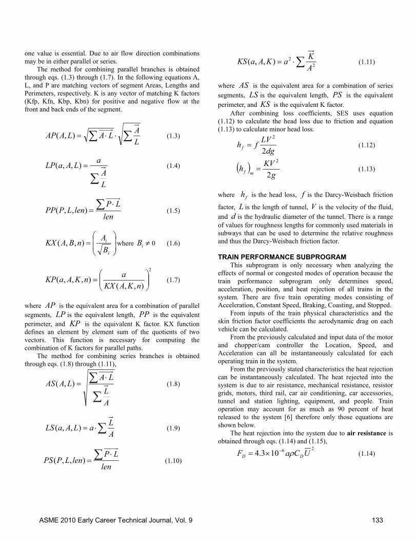
one value is essential. Due to air flow direction combinations may be in either parallel or series.

The method for combining parallel branches is obtained through eqs. (1.3) through (1.7). In the following equations A, L, and P are matching vectors of segment Areas, Lengths and Perimeters, respectively. K is any vector of matching K factors (Kfp, Kfn, Kbp, Kbn) for positive and negative flow at the front and back ends of the segment.

∑∑ ⋅⋅=LALALAAP ),( (1.3)

∑=

LA

aLAaLP ),,( (1.4)

lenLP

lenLPPP ∑ ⋅=),,( (1.5)

⎟⎟⎠

⎞⎜⎜⎝

⎛=

i

i

BAnBAKX ),,( where iB ≠ 0 (1.6)

2

),,(),,,( ⎟⎟

⎠

⎞⎜⎜⎝

⎛=

nKAKXanKAaKP (1.7)

where AP is the equivalent area for a combination of parallel segments, LP is the equivalent length, PP is the equivalent perimeter, and KP is the equivalent K factor. KX function defines an element by element sum of the quotients of two vectors. This function is necessary for computing the combination of K factors for parallel paths.

The method for combining series branches is obtained through eqs. (1.8) through (1.11),

∑

∑ ⋅=

AL

LALAAS ),( (1.8)

∑⋅=ALaLAaLS ),,( (1.9)

lenLP

lenLPPS ∑ ⋅=),,( (1.10)

∑⋅= 22),,(

AKaKAaKS (1.11)

where AS is the equivalent area for a combination of series segments, LS is the equivalent length, PS is the equivalent perimeter, and KS is the equivalent K factor.

After combining loss coefficients, SES uses equation (1.12) to calculate the head loss due to friction and equation (1.13) to calculate minor head loss.

dgLVfh f 2

2

= (1.12)

( )g

KVhmf 2

2

= (1.13)

where fh is the head loss, f is the Darcy-Weisbach friction

factor, L is the length of tunnel, V is the velocity of the fluid, and d is the hydraulic diameter of the tunnel. There is a range of values for roughness lengths for commonly used materials in subways that can be used to determine the relative roughness and thus the Darcy-Weisbach friction factor. TRAIN PERFORMANCE SUBPROGRAM

This subprogram is only necessary when analyzing the effects of normal or congested modes of operation because the train performance subprogram only determines speed, acceleration, position, and heat rejection of all trains in the system. There are five train operating modes consisting of Acceleration, Constant Speed, Braking, Coasting, and Stopped.

From inputs of the train physical characteristics and the skin friction factor coefficients the aerodynamic drag on each vehicle can be calculated.

From the previously calculated and input data of the motor and chopper/cam controller the Location, Speed, and Acceleration can all be instantaneously calculated for each operating train in the system.

From the previously stated characteristics the heat rejection can be instantaneously calculated. The heat rejected into the system is due to air resistance, mechanical resistance, resistor grids, motors, third rail, car air conditioning, car accessories, tunnel and station lighting, equipment, and people. Train operation may account for as much as 90 percent of heat released to the system [6] therefore only those equations are shown below.

The heat rejection into the system due to air resistance is obtained through eqs. (1.14) and (1.15),

26103.4 UCaF DD ρ−×= (1.14)


where DF is aerodynamic drag, ρ is the density of air, DC is

the aerodynamic drag coefficient, U is the average train velocity, and a is the frontal area of the train.

778ndFq bD

D = (1.15)

where Dq is the subway heat gain due to aerodynamic drag,

bd is the stopping distance from maximum speed (da can also

be used in place of bd and represents the distance to accelerate to maximum speed), and n is the number of trains through the station per hour.

The heat rejection into the system due to mechanical resistance is obtained through eqs. (1.16) and (1.17),

( )UW

FM4101.51163.1 −×++= (1.16)

where MF is the mechanical resistance force of a single car, W

is the weight of a single car including passengers, and U is the average train velocity.

778WNndFq bM

M = (1.17)

where Mq is the subway heat gain due to mechanical

resistance, MF is the mechanical resistance force of a single car, and N is the number of cars per train.

The heat rejection into the system due to the resistor grids is obtained through eq. (1.18),

KEqR = (1.18)

where Rq is the resistor heat rejected and KE is the kinetic energy.

The heat rejection into the system due to the car air conditioning is obtained through eq. (1.19),

tAC TNntq 51.4= (1.19)

where ACq is the subway heat gain due to the train air conditioning, T is the weight of the air conditioning units per car, and tt is the time for a single train to traverse the station.

From the previously stated characteristics the power demand can be instantaneously calculated. The power consumption can be divided into two parts: power consumption by auxiliary systems for an empty car and power consumption by auxiliary system per patron.

The power consumption due to an empty car is obtained through eq. (1.20),

IAACEAEC PPPPE++= (1.20)

where ECP is the power consumption by auxiliary systems for

an empty car, EAP is the power consumption by external

auxiliaries, EACP is the power consumption by air conditioning

equipment for an empty car, and IAP is the power consumption by internal auxiliaries.

The power consumption due to the patrons is obtained through eqs. (1.21) and (1.22),

IAACEALC PPPPL++= (1.21)

( )PFL

ECLCP N

PPP −= (1.22)

where LCP is the power consumption for a fully loaded car,

LACP is the power consumption by air conditioning equipment

for a loaded car, PP is the power consumption by auxiliary

systems per patron, and PFLN is the number of people aboard a fully loaded car. TEMPERATURE/HUMIDITY SUBPROGRAM

The temperature/humidity subprogram uses the airflow parameters and train heat release data to compute sensible and latent heat; thereby obtaining the temperature and humidity at all locations.

The input for outdoor ambient temperature for dry and wet bulb during both morning and evening conditions can be determined through the appropriate sources. Ambient temperatures for cooling are contained at 0.4% dry bulb conditions. Ambient temperatures for heating are contained at 99.6% dry bulb conditions. Determination of outdoor ambient temperature for morning and evening is found through the use of Table 1 and Table 2.

Table 1. Corrections for Time of Day [6]


Table 2. Corrections for Time of Year [6]

Table 1 contains corrections in outdoor design

temperatures for time of day. Table 2 contains corrections in outdoor design temperatures for time of year. With this data all ambient input temperatures can be inserted into the SES model. HEAT SINK/ENVIRONMENTAL CTRL SUBPROGRAM

The heat sink/environmental control subprogram uses the ventilation and heat load data, along with the daily and annual changes in outside conditions to compute the conduction of heat to the subway air, the structure, and the surrounding soil.

The tunnel wall and surrounding soil act as a heat sink. Because there is a temperature difference with the subway air flow and tunnel walls there is a transfer of energy [7]. From the previously stated characteristics the wall temperature can be instantaneously calculated with variations to equation (1.23) for heat transfer through conduction and equation (1.24) for heat transfer through convection.

( )L

Attkq Css 21 −= (1.23)

where q is the rate of heat transfer, k is the thermal

conductivity, ( )21 ss tt − is the difference in temperatures, A is

the area of the wall, and L is the wall thickness. ( )∞−= ttAhq SSC (1.24)

where Ch is the heat transfer coefficient, SA is the surface

area, and ( )∞− ttS is the difference in temperatures between the surface and ambient fluid.

FIRE EFFECTS SUBPROGRAM

The fire effects subprogram uses the resulting fire characteristics to determine the buoyancy in tunnels, throttling at the fire site, modified viscous flow losses, wall temperature, and radiation effects.

The temperature at the surface of the tunnel wall due to the thermal radiation effects of a fire can be obtained through variations to eq. (1.25),

4TWb σ= (1.25)

where bW is the blackbody emissive power and σ is the Stefan-Boltzmann constant.

The following, although not explicitly in SES, is important for the design engineer to consider when optimizing the ventilation system’s capacity. From the heat release rate and the previously stated characteristic the stratification of smoke can be determined [1]. The back layering distance due to the presence of a tunnel fire is obtained through eq. (1.26),

3/1

3 ⎟⎟⎠

⎞⎜⎜⎝

⎛∝

HuTcgQ

HL

apa

B

ρ (1.26)

where BL is back layering distance, H is the tunnel height,

Q is the heat release rate, aρ is the ambient density, aT is the ambient temperature, u is the air velocity, g is the acceleration

of gravity, and pc is the specific heat of air at constant

pressure. The average ‘cold’ gas velocity due to the presence of a

tunnel fire is obtained through eq. (1.27),

⎥⎥⎦

⎤

⎢⎢⎣

⎡⎟⎟⎠

⎞⎜⎜⎝

⎛−+++

⎟⎠⎞

⎜⎝⎛ −Δ

=

1

12

1a

sh

D

a

a

TTLL

DfK

TT

TThg

u (1.27)

where u is the ‘cold’ gas velocity, hΔ is the hot smoke stack

height, T is the average temperature over the hot stack height,

Df is the friction factor, L is the tunnel length, sL is the

length of the tunnel exposed to the hot smoke, hD is the

hydraulic diameter, and 1K is the pressure loss coefficient at the entrance of the tunnel.

Equations (1.26) and (1.27) help to determine whether or not back layering still persists in the presence of forced ventilation.

RESULTS

In order to better present the usefulness of SES, an example simulation is given below.

SES was used to determine the locations of fan and vent shafts and the size of the tunnel as part of a preliminary engineering analysis for the California High Speed Rail. Conceptual values for the tunnel roughness lengths, segment head loss coefficients, fan performance data, system geometry,


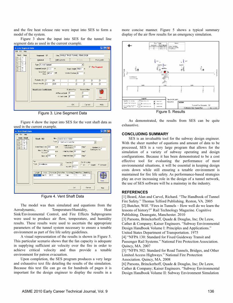
and the fire heat release rate were input into SES to form a model of the system.

Figure 3 show the input into SES for the tunnel line segment data as used in the current example.

Figure 3. Line Segment Data

Figure 4 show the input into SES for the vent shaft data as

used in the current example.

Figure 4. Vent Shaft Data

The model was then simulated and equations from the

Aerodynamic, Temperature/Humidity, Heat Sink/Environmental Control, and Fire Effects Subprograms were used to produce air flow, temperature, and humidity results. These results were used to ascertain the appropriate parameters of the tunnel system necessary to ensure a tenable environment as part of fire life safety guidelines.

A visual representation of the results is shown in Figure 5. This particular scenario shows that the fan capacity is adequate in supplying sufficient air velocity over the fire in order to achieve critical velocity and thus provide a tenable environment for patron evacuation.

Upon completion, the SES program produces a very large and exhaustive text file detailing the results of the simulation. Because this text file can go on for hundreds of pages it is important for the design engineer to display the results in a

more concise manner. Figure 5 shows a typical summary display of the air flow results for an emergency simulation.

Figure 5. Results

As demonstrated, the results from SES can be quite

exhaustive.

CONCLUDING SUMMARY SES is an invaluable tool for the subway design engineer.

With the sheer number of equations and amount of data to be processed, SES is a very large program that allows for the simulation of a variety of subway operating and design configurations. Because it has been demonstrated to be a cost effective tool for evaluating the performance of most environmental situations, it will be essential in keeping design costs down while still ensuring a tenable environment is maintained for fire life safety. As performance-based strategies play an ever increasing role in the design of a tunnel network, the use of SES software will be a mainstay in the industry.

REFERENCES [1] Beard, Alan and Carvel, Richard. “The Handbook of Tunnel Fire Safety.” Thomas Telford Publishing. Reston, VA. 2005 [2] Butcher, Wilf. “Fires in Tunnels – How well do we learn the lessons of history?” Rail Technology Magazine. Cognitive Publishing. Deansgate, Manchester. 2010 [3] Parsons, Brinckerhoff, Quade & Douglas, Inc; De Leuw, Cather & Company; Kaiser Engineers. “Subway Environmental Design Handbook Volume I: Principles and Applications.” United States Department of Transportation. 1975 [4] “NFPA 130: Standard for Fixed Guideway Transit and Passenger Rail Systems.” National Fire Protection Association. Quincy, MA. 2007 [5] “NFPA 502: Standard for Road Tunnels, Bridges, and Other Limited Access Highways.” National Fire Protection Association. Quincy, MA. 2008 [6] Parsons, Brinckerhoff, Quade & Douglas, Inc; De Leuw, Cather & Company; Kaiser Engineers. “Subway Environmental Design Handbook Volume II: Subway Environment Simulation


Computer Program Version 4.1.” United States Department of Transportation. 2001 [7] “ASHRAE Fundamentals Handbook 2009” American Society of Heating, Refrigerating, and Air-Conditioning Engineers, Inc. Atlanta, GA. 2009




TRAJECTORY PLANNING OF 3R ROBOTIC ARM USING GENETIC ALGORITHM (GA) AND ARTIFICIAL BEE COLONY (ABC) OPTIMIZATION METHODS

Savsani Poonam, Dr. Hemant Nagarsheth S.V. National Institute of Technology

Surat, Gujarat, INDIA

ABSTRACT In this paper two different evolutionary algorithms, the Artificial Bee Colony (ABC) and the Genetic algorithm (GA), are implemented for trajectory optimization of a three link robotic arm. The whole travel of the trajectory is divided into two parts, which consist of a fourth order polynomial trajectory for the one part and a fifth order trajectory for the second part. The objective function for the implemented algorithm is to minimize traveling time and space, while not exceeding a maximum pre-defined torque, in free workspace as well as circular obstacle existence robot workspace. The objective function consists of four parameters, viz. excessive driving torque, total joint traveling distance, total joint Cartesian length and total consumed time for robot motion. The results of ABC are compared with the published results of GA. Moreover one practical case was taken for the optimization of a human arm, considering it as a planar robotic arm, which was solved using ABC and GA. The comparison shows better performance of ABC over GA for the considered trajectory optimization problems. INTRODUCTION Robot arms are effectively used in modern production systems, and in order to achieve high-speed operation, optimal trajectory planning is extremely important. Thus many studies on optimal trajectory planning have been reported in free workspaces as well as in obstacle existence work spaces. The evolutionary algorithm is widely used as a practical optimization computation method, because this algorithm can avoid local minimum values and complicated theoretical computations. This work focused on the trajectory optimization of a 3R robotic arm in a free work space as well as a circular obstacle existence robot work space using both the ABC and the GA methods. Fourth-order and fifth-order polynomials are used to describe the segments that connect initial, intermediate and final points in the joint space. The results of ABC give a better

optimal trajectory in comparison with published results for GA. In recent years, evolutionary algorithms have been applied in a large number of fields. An optimal galloping trajectory was proposed by Giju and Jong [2] which cost low energy and which guaranteed the stability of the quadruped robot. Their optimized trajectory was based on energy and stability using GA, which provides a robust and global solution to a multi-body, highly nonlinear dynamic systems. For generating smooth trajectory planning for a specified path, Zoller and Zentan [3] focused on the problem of trajectory planning and dealt with constant kinetic energy motion planning. This method produced trajectory characteristics smoother and better than those obtained from the time optimal method. Zhe Tang et al. [6] proposed a third–order spline interpolation based on the trajectory-planning method to plan a smooth biped swing leg trajectory by reducing the instant velocity change. Garg and M. Kumar [8] used GA techniques for a robot arm to identify the optimal trajectory based on minimum joint torque requirements. The authors use a polynomial of 4th degree in time for trajectory representation to joint space variables. Pires and Machado [9] propose a path planning method based on a GA while adopting the direct kinematics and the inverse dynamics. The optimal trajectory is the one that minimizes the path length, the ripple in the time evolution and the energy requirements, without any collision with obstacles in the workspace. S. G. Yue et al. [4] focused on the problem of point-to-point trajectory planning of a flexible redundant robot manipulator (FRM) in joint space. The proposed trajectory to minimize vibration of FRMs is based on GA. Pires et al. [5] use a genetic algorithm to optimize a planar robot manipulator trajectory. In this line of thought, this work, proposes a point-to-point trajectory planning method based on GA while adopting the direct kinematics and the inverse dynamics.


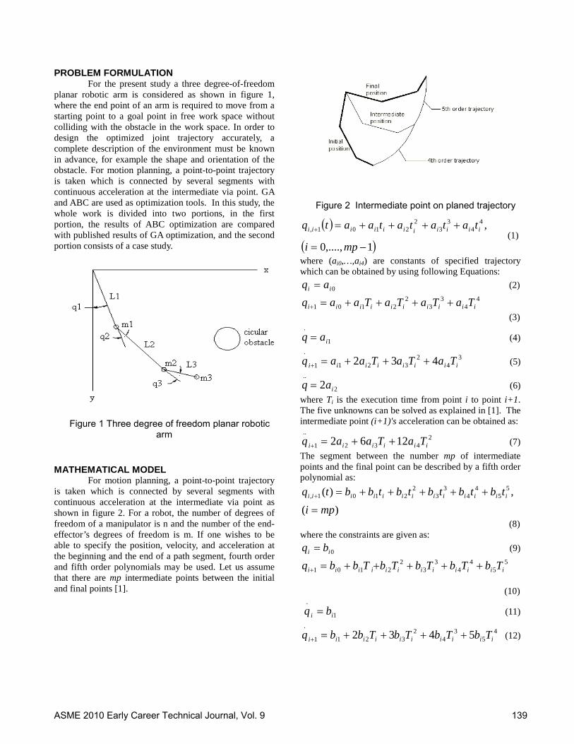
PROBLEM FORMULATION For the present study a three degree-of-freedom planar robotic arm is considered as shown in figure 1, where the end point of an arm is required to move from a starting point to a goal point in free work space without colliding with the obstacle in the work space. In order to design the optimized joint trajectory accurately, a complete description of the environment must be known in advance, for example the shape and orientation of the obstacle. For motion planning, a point-to-point trajectory is taken which is connected by several segments with continuous acceleration at the intermediate via point. GA and ABC are used as optimization tools. In this study, the whole work is divided into two portions, in the first portion, the results of ABC optimization are compared with published results of GA optimization, and the second portion consists of a case study.

Figure 1 Three degree of freedom planar robotic

arm

MATHEMATICAL MODEL For motion planning, a point-to-point trajectory is taken which is connected by several segments with continuous acceleration at the intermediate via point as shown in figure 2. For a robot, the number of degrees of freedom of a manipulator is n and the number of the end-effector’s degrees of freedom is m. If one wishes to be able to specify the position, velocity, and acceleration at the beginning and the end of a path segment, fourth order and fifth order polynomials may be used. Let us assume that there are mp intermediate points between the initial and final points [1].

Figure 2 Intermediate point on planed trajectory

( )( )1,....,0

,44

33

22101,

−=

++++=+

mpi

tatatataatq iiiiiiiiiii (1)

where (ai0,…,ai4) are constants of specified trajectory which can be obtained by using following Equations:

0ii aq = (2) 4

43

32

2101 iiiiiiiiii TaTaTaTaaq ++++=+ (3)

1

.

iaq = (4)

34

23211

.432 iiiiiiii TaTaTaaq +++=+ (5)

2

..2 iaq = (6)

where Ti is the execution time from point i to point i+1. The five unknowns can be solved as explained in [1]. The intermediate point (i+1)'s acceleration can be obtained as:

24321

..1262 iiiiii TaTaaq ++=+ (7)

The segment between the number mp of intermediate points and the final point can be described by a fifth order polynomial as:

)(,)( 5

54

43

32

2101,

mpitbtbtbtbtbbtq iiiiiiiiiiiii

=

+++++=+

(8) where the constraints are given as:

0ii bq = (9) 5

54

43

32

2101 iiiiiiiiiiii TbTbTbTbTbbq +++++=+

(10)

1

.

ii bq = (11)

45

34

23211

.5432 iiiiiiiiii TbTbTbTbbq ++++=+ (12)


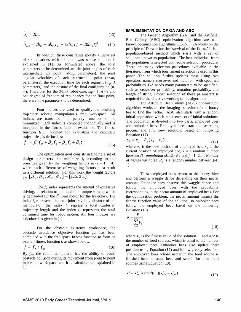
2

..2 ii bq = (13)

35

24321

..201262 iiiiiiii TbTbTbbq +++=+ (14)

In addition, these constraints specify a linear set of six equations with six unknowns whose solution is explained in [1]. As formulated above, the total parameters to be determined are the joint angles of each intermediate via point (n×mp parameters), the joint angular velocities of each intermediate point (n×mp parameters), the execution time for each segment (mp+1 parameters), and the posture of the final configuration (n-m). Therefore, for the 3-link robot case, mp= 1, n =3 and one degree of freedom of redundancy for the final point, there are nine parameters to be determined. Four indices are used to qualify the evolving trajectory robotic manipulator’s free workspace. All indices are translated into penalty functions to be minimized. Each index is computed individually and is integrated in the fitness function evaluation. The fitness function ff , adopted for evaluating the candidate trajectories, is defined as:

Tcqotf tffff 4321 ββββ +++= (15)

The optimization goal consists in finding a set of design parameters that minimize ff according to the priorities given by the weighting factors βi (i = 1,.., 4), where each different set of weighting factors must result in a different solution. For this work the weight factors are, [ ] [ ]1,2,2,1,,, 4321 =ββββ . The fot index represents the amount of excessive driving, in relation to the maximum torque τi max, which is demanded for the ith joint motor for the trajectory. The index fq represents the total joint traveling distance of the manipulator, the index fc represents total Cartesian trajectory length and the index tT represents the total consumed time for robot motion. All four indexes are calculated as given in [1]. For the obstacle existence workspace, the obstacle avoidance objective function fob has been combined with the free space fitness function to form an over all fitness function f, as shown below:

obf fff /= (16) By fob, the robot manipulator has the ability to avoid obstacle collision during its movement from point to point inside the workspace, and it is calculated as explained in [1].

IMPLEMENTATION OF GA AND ABC The Genetic Algorithm (GA) and the Artificial Bee Colony (ABC) optimization algorithm are well known optimization algorithms [11-15]. GA works on the principle of Darwin for the ‘survival of the fittest,’ It is a population-based method which starts with a set of solutions known as populations. The best individual from the population is selected with some selection procedure. There are many selection procedures available in the literature, from which tournament selection is used in this paper. The solution further updates these using two operators, namely crossover and mutation, with specified probabilities. GA needs many parameters to be specified, such as crossover probability, mutation probability, and length of string. Proper selection of these parameters is required for the effective working of the algorithm. The Artificial Bee Colony (ABC) optimization algorithm works on the foraging behavior of the honey bee to find the nectar. ABC also starts with a random initial population which represents set of initial solutions. The population is divided into two parts, employed bees and onlooker bees. Employed bees start the searching process and find new solutions based on following Equation (17).

(17) where vij is the new position of employed bee, xij is the current position of employed bee, k is a random number between (1, population size/2) ≠ i and j =1, 2,..., Number of design variables. Rij is a random number between (-1, 1). These employed bees return to the honey hive and perform a waggle dance depending on their nectar amount. Onlooker bees observe this waggle dance and follow the employed bees with the probability corresponding to the nectar amount of employed bees. For the optimization problem, the nectar amount mimics the fitness function value of the solution, so onlooker bees follow the employed bees based on the following Equation (18).

(18)

where Fi is the fitness value of the solution i, and N/2 is the number of food sources, which is equal to the number of employed bees. Onlooker bees also update their position using Equation (17) and follow greedy selection. The employed bees whose nectar in the food source is finished become scout bees and search for new food sources using Equation (19).

(19)

)( kjijijijij xxRxv −+=

∑=

= 2/

1

N

nn

ii

F

Fp

))(1,0( minmaxminjjjj

i xxrandxx −+=


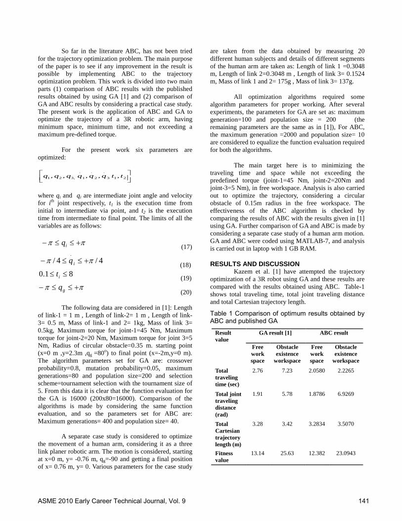
So far in the literature ABC, has not been tried for the trajectory optimization problem. The main purpose of the paper is to see if any improvement in the result is possible by implementing ABC to the trajectory optimization problem. This work is divided into two main parts (1) comparison of ABC results with the published results obtained by using GA [1] and (2) comparison of GA and ABC results by considering a practical case study. The present work is the application of ABC and GA to optimize the trajectory of a 3R robotic arm, having minimum space, minimum time, and not exceeding a maximum pre-defined torque.

For the present work six parameters are optimized:

213

.

2

.

1

.

,321 ,,,,, ttqqqqqq

where qi and qi are intermediate joint angle and velocity for ith joint respectively, t1 is the execution time from initial to intermediate via point, and t2 is the execution time from intermediate to final point. The limits of all the variables are as follows:

ππ +≤≤− iq (17)

4/4/.

ππ +≤≤− iq (18) 81.0 ≤≤ it (19)

ππ +≤≤− gq (20)

The following data are considered in [1]: Length of link-1 = 1 m , Length of link-2= 1 m , Length of link-3= 0.5 m, Mass of link-1 and 2= 1kg, Mass of link 3= 0.5kg, Maximum torque for joint-1=45 Nm, Maximum torque for joint-2=20 Nm, Maximum torque for joint 3=5 Nm, Radius of circular obstacle=0.35 m. starting point (x=0 m ,y=2.3m ,qg =80o) to final point (x=-2m,y=0 m). The algorithm parameters set for GA are: crossover probability=0.8, mutation probability=0.05, maximum generations=80 and population size=200 and selection scheme=tournament selection with the tournament size of 5. From this data it is clear that the function evaluation for the GA is 16000 (200x80=16000). Comparison of the algorithms is made by considering the same function evaluation, and so the parameters set for ABC are: Maximum generations= 400 and population size= 40. A separate case study is considered to optimize the movement of a human arm, considering it as a three link planer robotic arm. The motion is considered, starting at x=0 m, y= -0.76 m, qg=-90 and getting a final position of x= 0.76 m, y= 0. Various parameters for the case study

are taken from the data obtained by measuring 20 different human subjects and details of different segments of the human arm are taken as: Length of link 1 =0.3048 m, Length of link 2=0.3048 m , Length of link 3= 0.1524 m, Mass of link 1 and 2= 175g , Mass of link 3= 137g.

All optimization algorithms required some algorithm parameters for proper working. After several experiments, the parameters for GA are set as: maximum generation=100 and population size = 200 (the remaining parameters are the same as in [1]), For ABC, the maximum generation =2000 and population size= 10 are considered to equalize the function evaluation required for both the algorithms.

The main target here is to minimizing the traveling time and space while not exceeding the predefined torque (joint-1=45 Nm, joint-2=20Nm and joint-3=5 Nm), in free workspace. Analysis is also carried out to optimize the trajectory, considering a circular obstacle of 0.15m radius in the free workspace. The effectiveness of the ABC algorithm is checked by comparing the results of ABC with the results given in [1] using GA. Further comparison of GA and ABC is made by considering a separate case study of a human arm motion. GA and ABC were coded using MATLAB-7, and analysis is carried out in laptop with 1 GB RAM.

RESULTS AND DISCUSSION Kazem et al. [1] have attempted the trajectory optimization of a 3R robot using GA and these results are compared with the results obtained using ABC. Table-1 shows total traveling time, total joint traveling distance and total Cartesian trajectory length.

Table 1 Comparison of optimum results obtained by ABC and published GA

Result value

GA result [1] ABC result

Free work space

Obstacle existence

workspace

Free work space

Obstacle existence

workspace

Total traveling time (sec)

2.76 7.23 2.0580 2.2265

Total joint traveling distance (rad)

1.91 5.78 1.8786

6.9269

Total Cartesian trajectory length (m)

3.28 3.42 3.2834

3.5070

Fitness value

13.14 25.63 12.382 23.0943


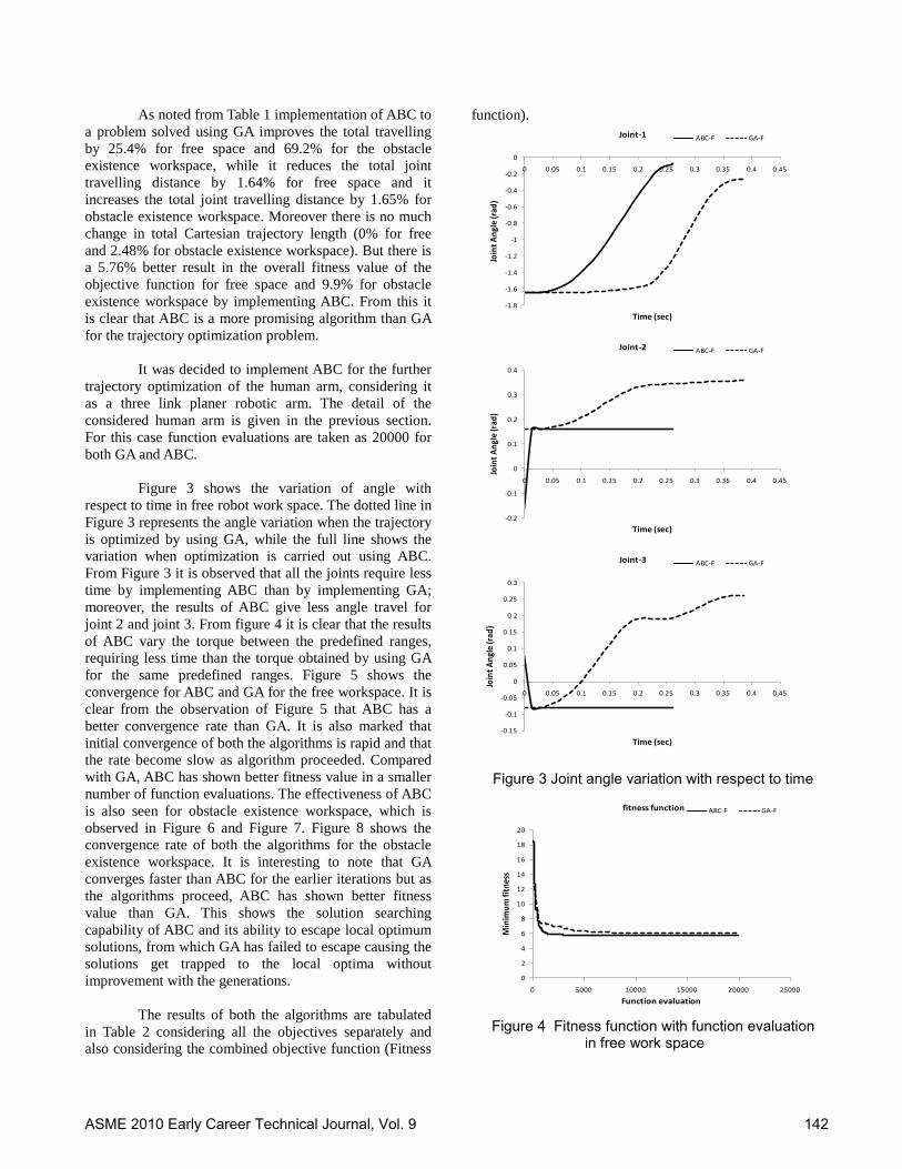
As noted from Table 1 implementation of ABC to a problem solved using GA improves the total travelling by 25.4% for free space and 69.2% for the obstacle existence workspace, while it reduces the total joint travelling distance by 1.64% for free space and it increases the total joint travelling distance by 1.65% for obstacle existence workspace. Moreover there is no much change in total Cartesian trajectory length (0% for free and 2.48% for obstacle existence workspace). But there is a 5.76% better result in the overall fitness value of the objective function for free space and 9.9% for obstacle existence workspace by implementing ABC. From this it is clear that ABC is a more promising algorithm than GA for the trajectory optimization problem. It was decided to implement ABC for the further trajectory optimization of the human arm, considering it as a three link planer robotic arm. The detail of the considered human arm is given in the previous section. For this case function evaluations are taken as 20000 for both GA and ABC. Figure 3 shows the variation of angle with respect to time in free robot work space. The dotted line in Figure 3 represents the angle variation when the trajectory is optimized by using GA, while the full line shows the variation when optimization is carried out using ABC. From Figure 3 it is observed that all the joints require less time by implementing ABC than by implementing GA; moreover, the results of ABC give less angle travel for joint 2 and joint 3. From figure 4 it is clear that the results of ABC vary the torque between the predefined ranges, requiring less time than the torque obtained by using GA for the same predefined ranges. Figure 5 shows the convergence for ABC and GA for the free workspace. It is clear from the observation of Figure 5 that ABC has a better convergence rate than GA. It is also marked that initial convergence of both the algorithms is rapid and that the rate become slow as algorithm proceeded. Compared with GA, ABC has shown better fitness value in a smaller number of function evaluations. The effectiveness of ABC is also seen for obstacle existence workspace, which is observed in Figure 6 and Figure 7. Figure 8 shows the convergence rate of both the algorithms for the obstacle existence workspace. It is interesting to note that GA converges faster than ABC for the earlier iterations but as the algorithms proceed, ABC has shown better fitness value than GA. This shows the solution searching capability of ABC and its ability to escape local optimum solutions, from which GA has failed to escape causing the solutions get trapped to the local optima without improvement with the generations. The results of both the algorithms are tabulated in Table 2 considering all the objectives separately and also considering the combined objective function (Fitness

function).

Figure 3 Joint angle variation with respect to time

Figure 4 Fitness function with function evaluation

in free work space

-1.8

-1.6

-1.4

-1.2

-1

-0.8

-0.6

-0.4

-0.2

0

0 0.05 0.1 0.15 0.2 0.25 0.3 0.35 0.4 0.45

Join

t Ang

le (r

ad)

Time (sec)

Joint-1 ABC-F GA-F

-0.2

-0.1

0

0.1

0.2

0.3

0.4

0 0.05 0.1 0.15 0.2 0.25 0.3 0.35 0.4 0.45

Join

t Ang

le (r

ad)

Time (sec)

Joint-2 ABC-F GA-F

-0.15

-0.1

-0.05

0

0.05

0.1

0.15

0.2

0.25

0.3

0 0.05 0.1 0.15 0.2 0.25 0.3 0.35 0.4 0.45

Join

t Ang

le (r

ad)

Time (sec)

Joint-3 ABC-F GA-F

0

2

4

6

8

10

12

14

16

18

20

0 5000 10000 15000 20000 25000

Min

imum

fitn

ess

Function evaluation

fitness function ABC-F GA-F


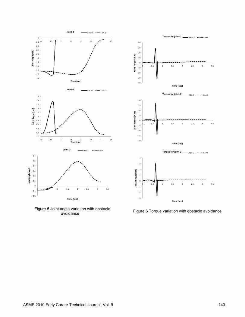
Figure 5 Joint angle variation with obstacle

avoidance

Figure 6 Torque variation with obstacle avoidance

-2

-1.8

-1.6

-1.4

-1.2

-1

-0.8

-0.6

-0.4

-0.2

0

0 0.5 1 1.5 2 2.5 3 3.5

Join

t Ang

le (r

ad)

Time (sec)

Joint-1 ABC-O GA-O

0

0.2

0.4

0.6

0.8

1

1.2

1.4

1.6

1.8

2

0 0.5 1 1.5 2 2.5 3 3.5

Join

t Ang

le (r

ad)

Time (sec)

Joint-2 ABC-O GA-O

-0.2

-0.1

0

0.1

0.2

0.3

0.4

0.5

0.6

0 0.5 1 1.5 2 2.5 3 3.5

Join

t Ang

le (r

ad)

Time (sec)

Joint-3 ABC-O GA-O

-40

-30

-20

-10

0

10

20

30

40

0 0.5 1 1.5 2 2.5 3 3.5

Join

t Tor

que(

N.m

)

Time (sec)

Torque for joint-1 ABC-O GA-O

-20

-15

-10

-5

0

5

10

15

20

0 0.5 1 1.5 2 2.5 3 3.5

Join

t Tor

que(

N.m

)

Time (sec)


-3

-2

-1

0

1

2

3

4

0 0.5 1 1.5 2 2.5 3 3.5

Join

t Tor

que(

N.m

)

Time (sec)



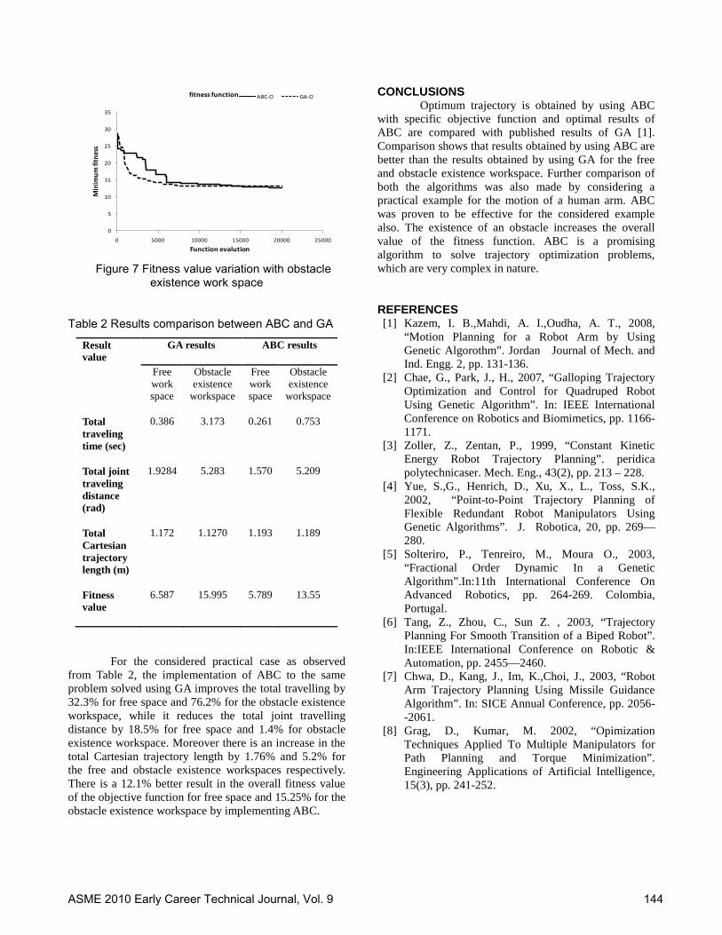
Figure 7 Fitness value variation with obstacle

existence work space

Table 2 Results comparison between ABC and GA

Result value

GA results ABC results

Free work space

Obstacle existence

workspace

Free work space

Obstacle existence

workspace

Total traveling time (sec)

0.386 3.173 0.261 0.753

Total joint traveling distance (rad)

1.9284 5.283 1.570 5.209

Total Cartesian trajectory length (m)

1.172 1.1270 1.193 1.189

Fitness value

6.587 15.995 5.789 13.55

For the considered practical case as observed from Table 2, the implementation of ABC to the same problem solved using GA improves the total travelling by 32.3% for free space and 76.2% for the obstacle existence workspace, while it reduces the total joint travelling distance by 18.5% for free space and 1.4% for obstacle existence workspace. Moreover there is an increase in the total Cartesian trajectory length by 1.76% and 5.2% for the free and obstacle existence workspaces respectively. There is a 12.1% better result in the overall fitness value of the objective function for free space and 15.25% for the obstacle existence workspace by implementing ABC.

CONCLUSIONS Optimum trajectory is obtained by using ABC with specific objective function and optimal results of ABC are compared with published results of GA [1]. Comparison shows that results obtained by using ABC are better than the results obtained by using GA for the free and obstacle existence workspace. Further comparison of both the algorithms was also made by considering a practical example for the motion of a human arm. ABC was proven to be effective for the considered example also. The existence of an obstacle increases the overall value of the fitness function. ABC is a promising algorithm to solve trajectory optimization problems, which are very complex in nature.

REFERENCES [1] Kazem, I. B.,Mahdi, A. I.,Oudha, A. T., 2008,

“Motion Planning for a Robot Arm by Using Genetic Algorothm”. Jordan Journal of Mech. and Ind. Engg. 2, pp. 131-136.

[2] Chae, G., Park, J., H., 2007, “Galloping Trajectory Optimization and Control for Quadruped Robot Using Genetic Algorithm”. In: IEEE International Conference on Robotics and Biomimetics, pp. 1166-1171.

[3] Zoller, Z., Zentan, P., 1999, “Constant Kinetic Energy Robot Trajectory Planning”. peridica polytechnicaser. Mech. Eng., 43(2), pp. 213 – 228.

[4] Yue, S.,G., Henrich, D., Xu, X., L., Toss, S.K., 2002, “Point-to-Point Trajectory Planning of Flexible Redundant Robot Manipulators Using Genetic Algorithms”. J. Robotica, 20, pp. 269—280.

[5] Solteriro, P., Tenreiro, M., Moura O., 2003, “Fractional Order Dynamic In a Genetic Algorithm”.In:11th International Conference On Advanced Robotics, pp. 264-269. Colombia, Portugal.

[6] Tang, Z., Zhou, C., Sun Z. , 2003, “Trajectory Planning For Smooth Transition of a Biped Robot”. In:IEEE International Conference on Robotic & Automation, pp. 2455—2460.

[7] Chwa, D., Kang, J., Im, K.,Choi, J., 2003, “Robot Arm Trajectory Planning Using Missile Guidance Algorithm”. In: SICE Annual Conference, pp. 2056--2061.

[8] Grag, D., Kumar, M. 2002, “Opimization Techniques Applied To Multiple Manipulators for Path Planning and Torque Minimization”. Engineering Applications of Artificial Intelligence, 15(3), pp. 241-252.

0

5

10

15

20

25

30

35

0 5000 10000 15000 20000 25000

Min

imum

fitn

ess

Function evalution

fitness function ABC-O GA-O


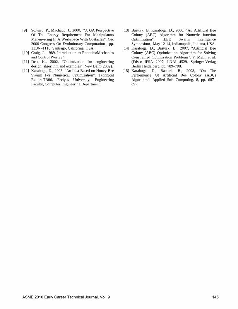
[9] Solteiro, P., Machado, J., 2000, “A GA Perspective Of The Energy Requirement For Manipulators Maneuvering In A Workspace With Obstacles”. Cec 2000-Congress On Evolutionary Computation , pp. 1110- -1116, Santiago, California, USA.

[10] Craig, J., 1989, Introduction to Robotics:Mechanics and Control.Wesley”

[11] Deb, K., 2002, “Optimization for engineering design: algorithm and examples”. New Delhi(2002).

[12] Karaboga, D., 2005, “An Idea Based on Honey Bee Swarm For Numerical Optimization”. Technical Report-TR06, Erciyes University, Engineering Faculty, Computer Engineering Department.

[13] Basturk, B. Karaboga, D., 2006, “An Artificial Bee Colony (ABC) Algorithm for Numeric function Optimization”. IEEE Swarm Intelligence Symposium, May 12-14, Indianapolis, Indiana, USA.

[14] Karaboga, D., Basturk, B., 2007, “Artificial Bee Colony (ABC) Optimization Algorithm for Solving Constrained Optimization Problems”. P. Melin et al. (Eds.): IFSA 2007, LNAI 4529, Springer-Verlag Berlin Heidelberg. pp. 789–798.

[15] Karaboga, D., Basturk, B., 2008, “On The Performance Of Artificial Bee Colony (ABC) Algorithm”. Applied Soft Computing. 8, pp. 687–697.




MULTI-OBJECTIVE OPTIMIZATION OF MECHANICAL ELEMENTS USING ARTIFICIAL BEE COLONY OPTIMIZATION TECHNIQUE

Savsani Vimal, Dr. R.V. Rao, Dr. D.P.Vakharia S.V. National Institute of Technology

Surat, Gujarat, INDIA

ABSTRACT Bearings and gears are very important components of any mechanical system. The multi-objective optimization of a single row deep groove ball bearing and gear box is presented in this paper. Three different objectives are considered viz. dynamic capacity, static capacity and elastohydrodynamic minimum film thickness for ball bearings, and optimization is carried out considering two objectives and three objectives simultaneously. Two stage and three stage gear boxes are considered for multi-objective optimizations which consists of two objectives, viz. surface fatigue life and minimum volume. An artificial bee colony (ABC) optimization technique is used to solve optimization problems. The results of optimization using the ABC technique are compared with the results of other optimization techniques.

INTRODUCTION Rolling bearings are widely used as an important component in most mechanical and aerospace engineering applications. Continuous advancement in the design of bearing is seen for house-hold appliance, automotive, space, aeronautical, micro- or nano-machine applications. This has motivated design engineers to come up with a design technology that gives long lasting, more efficient and highly reliable bearing design. A rolling-element bearing is a bearing which carries a load by placing round elements between two pieces. A common kind of rolling-element bearing is the ball bearing. The bearing has inner and outer races and a set of balls. Each race is a ring with a groove where the balls rest. The groove is usually shaped so the ball is a slightly loose fit in the groove. The ball contacts each race at a single point. In actual practice, the ball deforms slightly where it contacts each race. The race also dents slightly where each ball presses on it. Thus, the contact between ball and race is of finite size and has finite pressure. Because of this deformation of balls, there is little sliding with pure rolling.

All parts of a bearing are subject to many design constraints. For example, the inner and outer races are of complex shapes which make them difficult to design and manufacture. Balls and rollers, though simpler in shape, are small; since they bend sharply where they run on the races, the bearings are prone to fatigue. The loads within a bearing assembly are also affected by the speed of operation. Techniques for minimum volume design of simple and multiple –stage gear boxes have been a subject of interest to researchers because many high performance power transmission applications, such as those in the automotive and aerospace industries, require low weight. Conventional design determines the value of diametral pitch at which tooth bending fatigue failure and surface fatigue failure are equally likely. For cyclic loading in simple bending, ferrous metals exhibit the well known endurance limit phenomenon, and hence infinite fatigue life with respect to the bending load is theoretically possible. However the Hertz contact stress occurring on the tooth surface represents a state of tri-axial stress which in cyclic loading does not exhibit the same endurance limit characteristics. Therefore a specified lifetime in surface fatigue must be assumed, which affects the subsequent calculations. The approach in this paper is to extend the procedure by studying the tradeoff between surface fatigue life and minimum volume using a multi-objective optimization technique. This approach is very useful to determine the optimum selection of a number of stages according to the required multi-objectives. ARTIFICIAL BEE COLONY (ABC) TECHNIQUE The Artificial Bee Colony (ABC) Algorithm is an optimization algorithm based on the intelligent foraging behaviour of honey bee swarms. The colony of artificial bees consists of three groups of bees: employed bees, onlookers and scouts [1, 2]. Employed bee searches the destination where food is available. They collect the food


http://en.wikipedia.org/wiki/Bearing_%28mechanical%29�

http://en.wikipedia.org/wiki/Ball_bearing�

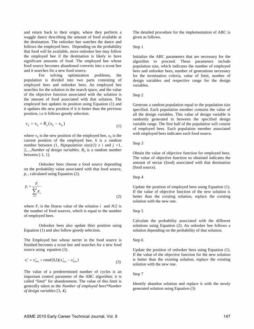
and return back to their origin, where they perform a waggle dance describing the amount of food available at the destination. The onlooker bee watches the dance and follows the employed bees. Depending on the probability that food will be available, more onlooker bee may follow the employed bee if the destination is likely to have significant amounts of food. The employed bee whose food source becomes abandoned converts into a scout bee and it searches for a new food source. For solving optimization problems, the population is divided into two parts consisting of employed bees and onlooker bees. An employed bee searches for the solution in the search space, and the value of the objective function associated with the solution is the amount of food associated with that solution. The employed bee updates its position using Equation (1) and it updates the new position if it is better than the previous position, i.e it follows greedy selection.

)( kjijijijij xxRxv −+= (1) where vij is the new position of the employed bee, xij is the current position of the employed bee, k is a random number between (1, N(population size)/2) ≠ i and j =1, 2,...,Number of design variables. Rij is a random number between (-1, 1). Onlooker bees choose a food source depending on the probability value associated with that food source, pi , calculated using Equation (2).

∑=

= 2/

1

N

nn

ii

F

Fp

(2)

where Fi is the fitness value of the solution i and N/2 is the number of food sources, which is equal to the number of employed bees.

Onlooker bees also update thier position using Equation (1) and also follow greedy selection.

The Employed bee whose necter in the food source is finished becomes a scout bee and searches for a new food source using equation (3).

))(1,0( minmaxminjjjj

i xxrandxx −+= (3)

The value of a predetermined number of cycles is an important control parameter of the ABC algorithm; it is called “limit” for abandonment. The value of this limit is generally taken as the Number of employed bees*Number of design variables [3, 4].

The detailed procedure for the implementation of ABC is given as follows.

Step 1

Initialize the ABC parameters that are necessary for the algorithm to proceed. These parameters include population size, which indicates the number of employed bees and onlooker bees, number of generations necessary for the termination criteria, value of limit, number of design variables and respective range for the design variables.

Step 2

Generate a random population equal to the population size specified. Each population member contains the value of all the design variables. This value of design variable is randomly generated in between the specified design variable range. The first half of the population will consist of employed bees. Each population member associated with employed bees indicates each food source.

Step 3

Obtain the value of objective function for employed bees. The value of objective function so obtained indicates the amount of nectar (food) associated with that destination (food source).

Step 4

Update the position of employed bees using Equation (1). If the value of objective function of the new solution is better than the existing solution, replace the existing solution with the new one.

Step 5

Calculate the probability associated with the different solutions using Equation (2). An onlooker bee follows a solution depending on the probability of that solution.

Step 6

Update the position of onlooker bees using Equation (1). If the value of the objective function for the new solution is better than the existing solution, replace the existing solution with the new one.

Step 7

Identify abandon solution and replace it with the newly generated solution using Equation (3)


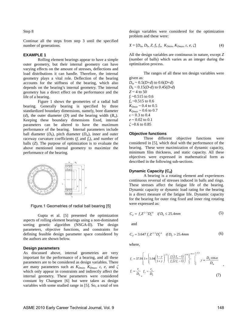
Step 8

Continue all the steps from step 3 until the specified number of generations.

EXAMPLE 1 Rolling element bearings appear to have a simple outer geometry, but their internal geometry can have varying effects on the amount of stresses, deflections and load distributions it can handle. Therefore, the internal geometry plays a vital role. Deflection of the bearing accounts for the stiffness of the bearing, which also depends on the bearing’s internal geometry. The internal geometry has a direct effect on the performance and the life of a bearing. Figure 1 shows the geometries of a radial ball bearing. Generally bearing is specified by three standardized boundary dimensions, namely, bore diameter (d), the outer diameter (D) and the bearing width (Bw). Keeping these boundary dimensions fixed, internal parameters can be altered to have the maximum performance of the bearing. Internal parameters include ball diameter (Db), pitch diameter (Dm), inner and outer raceway curvature coefficients (fi and fo), and number of balls (Z). The purpose of optimization is to evaluate the above mentioned internal geometry to maximize the performance of the bearing.

Figure.1 Geometries of radial ball bearing [5]

Gupta et al. [5] presented the optimization aspects of rolling element bearings using a non-dominated sorting genetic algorithm (NSGA-II). The design parameters, objective functions, and constraints for defining feasible design parameter space considered by the authors are shown below.

Design parameters As discussed above, internal geometries are very important for the performance of a bearing, and all these parameters are to be considered as design variables. There are many parameters such as KDmin, KDmax, ε, e, and ζ which only appear in constraints and indirectly affect the internal geometry. These parameters were considered constant by Changsen [6] but were taken as design variables with some studied range in [5]. So, a total of ten

design variables were considered for the optimization problem and these were: X = [Dm, Db, Z, fi, fo, KDmin, KDmax, ε, e, ζ] (4) All the design variables are continuous in nature, except Z (number of balls) which varies as an integer during the optimization process. The ranges of all these ten design variables were given as: Dm ~ 0.5(D+d) to 0.6(D+d) Db ~ 0.15(D-d) to 0.45(D-d) Z ~ 4 to 50 fi ~0.515 to 0.6 fo ~0.515 to 0.6 KDmin ~ 0.4 to 0.5 KDmax ~ 0.6 to 0.7 ε ~ 0.3 to 0.4 e ~ 0.02 to 0.1 ζ ~0.6 to 0.85 Objective functions Three different objective functions were considered in [5], which deal with the performance of the bearing. These were maximization of dynamic capacity, minimum film thickness, and static capacity. All these objectives were expressed in mathematical form as described in the following sub-sections.

Dynamic Capacity (Cd) A bearing is a rotating element and experiences continuous reversal of stresses induced in balls and rings. These stresses affect the fatigue life of the bearing. Dynamic capacity or dynamic load rating for the bearing is a direct measure of the fatigue life. Dynamic capacity for the bearing for outer ring fixed and inner ring rotating were expressed as:

mmDifDZfC bbcd 4.258.13/2 ≤= (5)

and

mmDifDZfC bbcd 4.25647.3 4.13/2 >= (6)

where,

( )( )

3.03/1041.072.1

1212

1104.1191.37

−

−−

+−

+=io

oic ff

fff

γγ

m

b

DD α

γcos

= ,

b

ii D

rf =

, b

oo D

rf =

(7)


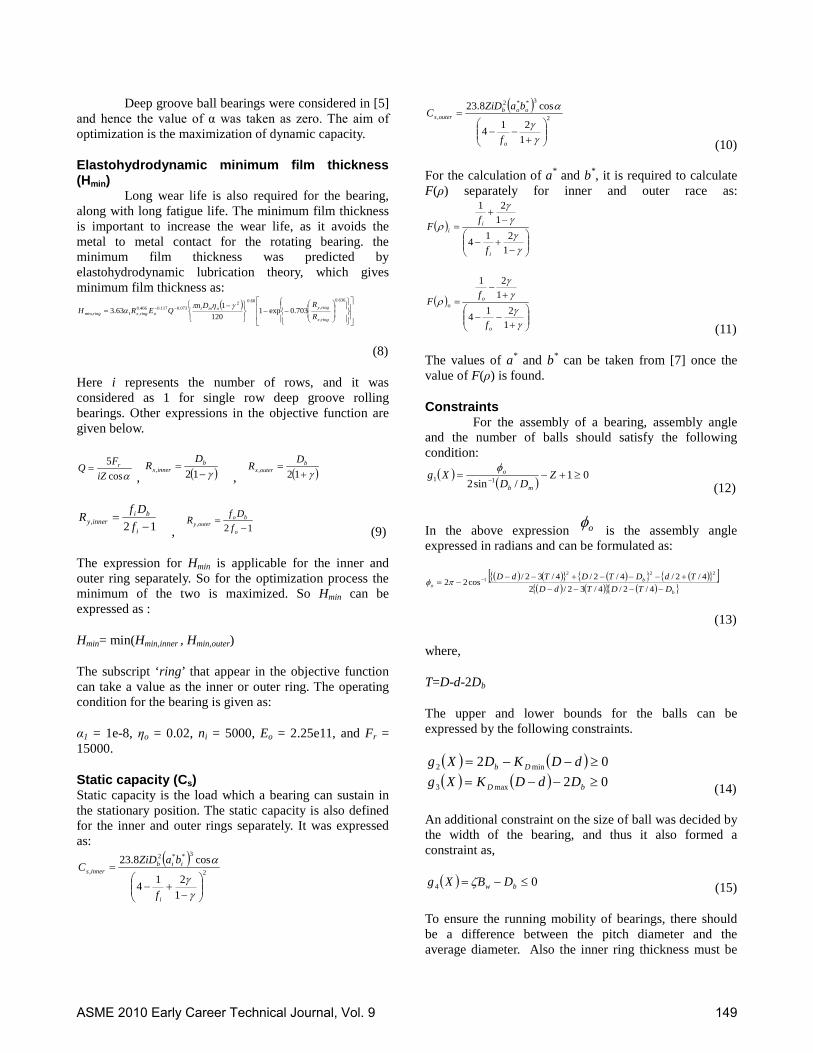
Deep groove ball bearings were considered in [5] and hence the value of α was taken as zero. The aim of optimization is the maximization of dynamic capacity.

Elastohydrodynamic minimum film thickness (Hmin) Long wear life is also required for the bearing, along with long fatigue life. The minimum film thickness is important to increase the wear life, as it avoids the metal to metal contact for the rotating bearing. the minimum film thickness was predicted by elastohydrodynamic lubrication theory, which gives minimum film thickness as:

( )

−−

−

= −−

636.0

,

,68.02

073.0117.0466.0,1min, 703.0exp1

1201

63.3ringx

ringyomioringxring R

RDnQERH

γηπα

(8)

Here i represents the number of rows, and it was considered as 1 for single row deep groove rolling bearings. Other expressions in the objective function are given below.

αcos5

iZFQ r=

, ( )γ−=12,

binnerx

DR

, ( )γ+=12,

bouterx

DR

12, −=

i

biinnery f

DfR

, 12, −=

o

booutery f

DfR

(9)

The expression for Hmin is applicable for the inner and outer ring separately. So for the optimization process the minimum of the two is maximized. So Hmin can be expressed as :

Hmin= min(Hmin,inner , Hmin,outer)

The subscript ‘ring’ that appear in the objective function can take a value as the inner or outer ring. The operating condition for the bearing is given as:

α1 = 1e-8, ηo = 0.02, ni = 5000, Eo = 2.25e11, and Fr = 15000.

Static capacity (Cs) Static capacity is the load which a bearing can sustain in the stationary position. The static capacity is also defined for the inner and outer rings separately. It was expressed as:

( )2

3**2

,

1214

cos8.23

−

+−

=

γγ

α

i

iibinners

f

baZiDC

( )2

3**2

,

1214

cos8.23

+

−−

=

γγ

α

o

oobouters

f

baZiDC

(10) For the calculation of a* and b*, it is required to calculate F(ρ) separately for inner and outer race as:

( )

−

+−

−+

=

γγγγ

ρ

1214

121

i

ii

f

fF

( )

+

−−

+−

=

γγγγ

ρ

1214

121

o

oo

f

fF

(11)

The values of a* and b* can be taken from [7] once the value of F(ρ) is found.

Constraints For the assembly of a bearing, assembly angle and the number of balls should satisfy the following condition:

( ) ( ) 01/sin2 11 ≥+−= − ZDD

Xgmb

oφ

(12)

In the above expression oφ is the assembly angle expressed in radians and can be formulated as:

( ) ( ){ } ( ){ } ( ){ }[ ]( ) ( ){ } ( ){ }b

bo DTDTdD

TdDTDTdD−−−−

+−−−+−−−= −

4/2/4/32/24/2/4/2/4/32/

cos22222

1πφ

(13)

where,

T=D-d-2Db

The upper and lower bounds for the balls can be expressed by the following constraints.

( ) ( ) 02 min2 ≥−−= dDKDXg Db ( ) ( ) 02max3 ≥−−= bD DdDKXg (14)

An additional constraint on the size of ball was decided by the width of the bearing, and thus it also formed a constraint as,

( ) 04 ≤−= bw DBXg ζ (15)

To ensure the running mobility of bearings, there should be a difference between the pitch diameter and the average diameter. Also the inner ring thickness must be


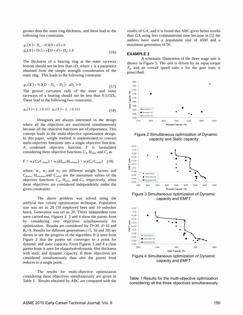
greater than the outer ring thickness, and these lead to the following two constraints.

( ) ( ) 05.05 ≥+−= dDDXg m

( ) ( )( ) 05.06 ≥−++= mDdDeXg (16)

The thickness of a bearing ring at the outer raceway bottom should not be less than εD, where ε is a parameter obtained from the simple strength consideration of the outer ring. This leads to the following constraint:

( ) ( ) 05.07 ≥−−−= bbm DDDDXg ε (17) The groove curvature radii of the inner and outer raceways of a bearing should not be less than 0.515Db. These lead to the following two constraints.

( ) 515.08 ≥= ifXg ( ) 515.09 ≥= ofXg (18)

Designers are always interested in the design where all the objectives are maximized simultaneously because all the objective functions are of importance. This concept leads to the multi-objective optimization design. In this paper, weight method is implemented to convert multi-objective functions into a single objective function. A combined objective function F is formulated considering three objective functions Cd, Hmin, and Cs as

F = w1(Cd/Cdmax) + w2(Hmin/Hminmax) + w3(Cs/Csmax) (19)

where, w1, w2 and w3 are different weight factors and Cdmax, Hminmax,and Csmax are the maximum values of the objective functions Cd, Hmin, and Cs, respectively, when these objectives are considered independently under the given constraints.

The above problem was solved using the artificial bee colony optimization technique. Population size was set as 20 (10 employed bees and 10 onlooker bees). Generation was set as 20. Thirty independent runs were carried out. Figures 2, 3 and 4 show the pareto front by considering two objectives simultaneously for optimization. Results are considered for D=30, d=10 and Bw=9. Results for different generations (=5, 10 and 20) are shown to see the progress of the algorithm. It is seen from Figure 2 that the pareto set converges to a point for dynamic and static capacity. From Figures 3 and 4 a clear pareto front is seen for elastohydrodynamic film thickness with static and dynamic capacity. If three objectives are considered simultaneously than also the pareto front reduces to a single point.

The results for multi-objective optimization considering three objectives simultaneously are given in Table 1. Results obtained by ABC are compared with the

results of GA, and it is found that ABC gives better results than GA using less computational time because in [5] the authors have used a population size of 4500 and a maximum generation of 50.

EXAMPLE 2 A schematic illustration of the three stage unit is shown in Figure 5. The unit is driven by an input torque Tin and an overall speed ratio e for the gear train is prescribed.

Figure.2 Simultaneous optimization of Dynamic capacity and Static capacity

Figure.3 Simultaneous optimization of Dynamic capacity and EMFT

Figure.4 Simultaneous optimization of Dynamic capacity and EMFT

Table 1 Results for the multi-objective optimization considering all the three objectives simultaneously

3620

3640

3660

3680

3700

3720

3740

3760

3780

3800

5750 5800 5850 5900 5950 6000 6050

Stat

ic C

apac

ity (

N)

Dynamic Capacity (N)

Generation-5

Generation-10

Generation-20

0.202

0.204

0.206

0.208

0.21

0.212

0.214

0.216

0.218

0.22

0.222

2500 3000 3500 4000 4500 5000 5500 6000 6500

EM

FT (μm

)

Dynamic Capacity (N)

Generation-5

Generation-10

Generation-20

0.202

0.204

0.206

0.208

0.21

0.212

0.214

0.216

0.218

0.22

0.222

2000 2500 3000 3500 4000

EM

FT (μm

)

Static Capacity (N)

Generation-5

Generation-10

Generation-20


_____________________________________________________________________

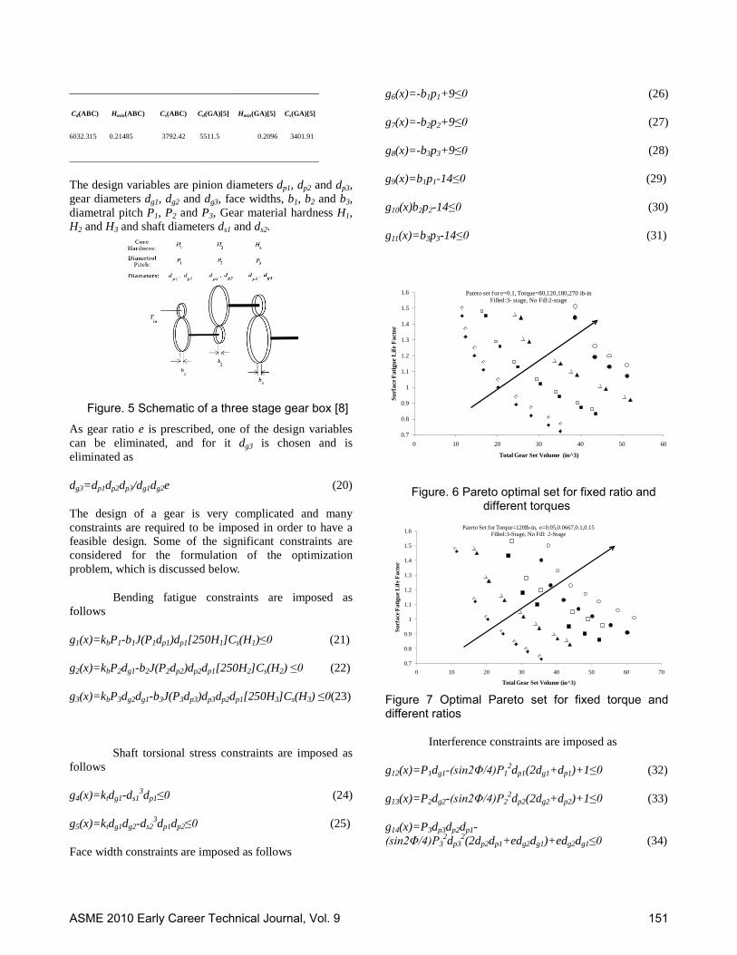
Cd(ABC) Hmin(ABC) Cs(ABC) Cd(GA)[5] Hmin(GA)[5] Cs(GA)[5]

6032.315 0.21485 3792.42 5511.5 0.2096 3401.91

_____________________________________________________________________

The design variables are pinion diameters dp1, dp2 and dp3, gear diameters dg1, dg2 and dg3, face widths, b1, b2 and b3, diametral pitch P1, P2 and P3, Gear material hardness H1, H2 and H3 and shaft diameters ds1 and ds2.

Figure. 5 Schematic of a three stage gear box [8]

As gear ratio e is prescribed, one of the design variables can be eliminated, and for it dg3 is chosen and is eliminated as

dg3=dp1dp2dp3/dg1dg2e (20)

The design of a gear is very complicated and many constraints are required to be imposed in order to have a feasible design. Some of the significant constraints are considered for the formulation of the optimization problem, which is discussed below.

Bending fatigue constraints are imposed as follows

g1(x)=kbP1-b1J(P1dp1)dp1[250H1]Cs(H1)≤0 (21)

g2(x)=kbP2dg1-b2J(P2dp2)dp2dp1[250H2]Cs(H2) ≤0 (22)

g3(x)=kbP3dg2dg1-b3J(P3dp3)dp3dp2dp1[250H3]Cs(H3) ≤0(23)

Shaft torsional stress constraints are imposed as follows

g4(x)=ktdg1-ds13dp1≤0 (24)

g5(x)=ktdg1dg2-ds23dp1dp2≤0 (25)

Face width constraints are imposed as follows

g6(x)=-b1p1+9≤0 (26)

g7(x)=-b2p2+9≤0 (27)

g8(x)=-b3p3+9≤0 (28)

g9(x)=b1p1-14≤0 (29)

g10(x)b2p2-14≤0 (30)

g11(x)=b3p3-14≤0 (31)

Figure. 6 Pareto optimal set for fixed ratio and different torques

Figure 7 Optimal Pareto set for fixed torque and different ratios

Interference constraints are imposed as

g12(x)=P1dg1-(sin2Φ/4)P12dp1(2dg1+dp1)+1≤0 (32)

g13(x)=P2dg2-(sin2Φ/4)P22dp2(2dg2+dp2)+1≤0 (33)

g14(x)=P3dp3dp2dp1-(sin2Φ/4)P3

2dp32(2dp2dp1+edg2dg1)+edg2dg1≤0 (34)

0.7

0.8

0.9

1

1.1

1.2

1.3

1.4

1.5

1.6

0 10 20 30 40 50 60

Surf

ace F

atig

ue L

ife F

acto

r

Total Gear Set Volume (in^3)

Pareto set for e=0.1, Torque=80,120,180,270 ib-in Filled:3- stage, No Fill:2-stage

0.7

0.8

0.9

1

1.1

1.2

1.3

1.4

1.5

1.6

0 10 20 30 40 50 60 70

Surf

ace F

atig

ue L

ife F

acto

r

Total Gear Set Volume (in^3)

Pareto Set for Torque=120lb-in, e=0.05,0.0667,0.1,0.15Filled:3-Stage, No Fill: 2-Stage


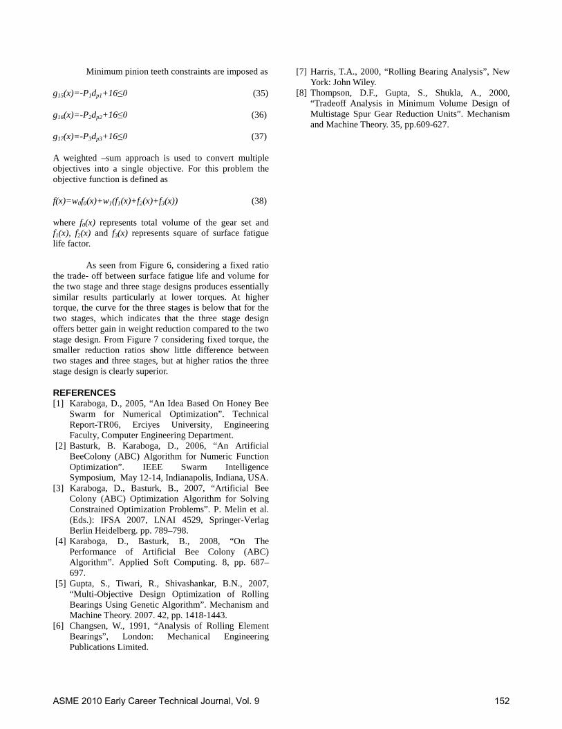
Minimum pinion teeth constraints are imposed as

g15(x)=-P1dp1+16≤0 (35)

g16(x)=-P2dp2+16≤0 (36)

g17(x)=-P3dp3+16≤0 (37)

A weighted –sum approach is used to convert multiple objectives into a single objective. For this problem the objective function is defined as

f(x)=w0f0(x)+w1(f1(x)+f2(x)+f3(x)) (38)

where f0(x) represents total volume of the gear set and f1(x), f2(x) and f3(x) represents square of surface fatigue life factor.

As seen from Figure 6, considering a fixed ratio the tradeoff between surface fatigue life and volume for the two stage and three stage designs produces essentially similar results particularly at lower torques. At higher torque, the curve for the three stages is below that for the two stages, which indicates that the three stage design offers better gain in weight reduction compared to the two stage design. From Figure 7 considering fixed torque, the smaller reduction ratios show little difference between two stages and three stages, but at higher ratios the three stage design is clearly superior.

REFERENCES [1] Karaboga, D., 2005, “An Idea Based On Honey Bee

Swarm for Numerical Optimization”. Technical Report-TR06, Erciyes University, Engineering Faculty, Computer Engineering Department.

[2] Basturk, B. Karaboga, D., 2006, “An Artificial BeeColony (ABC) Algorithm for Numeric Function Optimization”. IEEE Swarm Intelligence Symposium, May 12-14, Indianapolis, Indiana, USA.

[3] Karaboga, D., Basturk, B., 2007, “Artificial Bee Colony (ABC) Optimization Algorithm for Solving Constrained Optimization Problems”. P. Melin et al. (Eds.): IFSA 2007, LNAI 4529, Springer-Verlag Berlin Heidelberg. pp. 789–798.

[4] Karaboga, D., Basturk, B., 2008, “On The Performance of Artificial Bee Colony (ABC) Algorithm”. Applied Soft Computing. 8, pp. 687–697.

[5] Gupta, S., Tiwari, R., Shivashankar, B.N., 2007, “Multi-Objective Design Optimization of Rolling Bearings Using Genetic Algorithm”. Mechanism and Machine Theory. 2007. 42, pp. 1418-1443.

[6] Changsen, W., 1991, “Analysis of Rolling Element Bearings”, London: Mechanical Engineering Publications Limited.

[7] Harris, T.A., 2000, “Rolling Bearing Analysis”, New York: John Wiley.

[8] Thompson, D.F., Gupta, S., Shukla, A., 2000, “Tradeoff Analysis in Minimum Volume Design of Multistage Spur Gear Reduction Units”. Mechanism and Machine Theory. 35, pp.609-627.


Documents

INTERACTIVE COMPUTATIONAL TOOL FOR SIMULATION OF … · 2018-07-24 · Newmark integration (δ=0.25, γ=0.5, ... versus nodal displacement vector (Fig.5) for cross sections located