Interactive molecular dynamics

Daniel V. Schroedera)

Physics Department, Weber State University, Ogden, Utah 84408-2508

(Received 6 August 2014; accepted 27 October 2014)

Physics students now have access to interactive molecular dynamics simulations that can model

and animate the motions of hundreds of particles, such as noble gas atoms, that attract each other

weakly at short distances but repel strongly when pressed together. Using these simulations,

students can develop an understanding of forces and motions at the molecular scale, nonideal

fluids, phases of matter, thermal equilibrium, nonequilibrium states, the Boltzmann distribution, the

arrow of time, and much more. This article summarizes the basic features and capabilities of such a

simulation, presents a variety of student exercises using it at the introductory and intermediate

levels, and describes some enhancements that can further extend its uses. A working simulation

code, in HTML5 and JAVASCRIPT for running within any modern Web browser, is provided as an

online supplement. VC 2015 American Association of Physics Teachers.

[http://dx.doi.org/10.1119/1.4901185]

I. INTRODUCTION

The atomic theory of matter is a pillar of modern science.Richard Feynman said it best:1–3

If, in some cataclysm, all of scientific knowledgewere to be destroyed, and only one sentence passedon to the next generations of creatures, what state-ment would contain the most information in thefewest words? I believe it is the atomic hypothesis(or the atomic fact, or whatever you wish to call it)that all things are made of atoms—little particlesthat move around in perpetual motion, attractingeach other when they are a little distance apart,but repelling upon being squeezed into oneanother. In that one sentence, you will see, there isan enormous amount of information about theworld, if just a little imagination and thinking areapplied.

Experienced physicists can readily apply “just a littleimagination and thinking” to this view of matter, to arrive ata qualitative, microscopic understanding of gas pressure,phase changes, thermal equilibrium, nonequilibrium states,irreversible behavior, and specific phenomena such as fric-tion, thermal expansion, surface tension, crystal dislocations,and Brownian motion. With further analysis and calculation,physicists can also quantify much of this understanding interms of the laws of thermodynamics, Boltzmann statistics,kinetic theory, and so on.

Non-experts, however, do not automatically imagine andthink about these phenomena correctly. For example, manystudents find it difficult to picture atoms in perpetual motion,colliding elastically with no loss of energy over time—eventhough this picture is essential to understanding how a gascan exert a steady pressure.4–6 Physics students graduallylearn quantitative approaches to thermodynamics and statis-tical mechanics, but their qualitative understanding can lagbehind their symbol-pushing skills. Moreover, at the under-graduate level, the thermal physics curriculum tends to berestricted to a disappointingly narrow range of systems:

• “ideal” gases in which the particles do not attract or repeleach other at all; and/or

• systems in equilibrium (so that the fundamental assump-tion of statistical mechanics applies); and/or

• very large systems (in the “thermodynamic limit”), forwhich fluctuations and surface effects are negligible.

Of course, these restrictions are usually necessary in order toperform accurate pencil-and-paper calculations.

To study systems that are free of these restrictions,researchers often use molecular dynamics simulations.7–9 Intheir basic form, these simulations integrate Newton’s sec-ond law numerically to determine the motions of a moder-ately large number of classical particles. In this approach,there is no difficulty with incorporating forces between theparticles, or with studying nonequilibrium states. Simulatingvery large systems is computationally expensive, so fluctua-tions and surface effects are necessarily apparent (for betteror for worse) in practical simulations.

Molecular dynamics is gradually making its way into sci-ence education, from two directions. At the elementary level,there are now simulations with animated graphics that areintended to give precollege students and chemistry students aqualitative understanding of the atomic view of matter, andespecially of the differences between solids, liquids, andgases.10–14 Meanwhile, at a more advanced level, a growingnumber of text materials15–18 for computational physics andstatistical physics are presenting molecular dynamics tem-plate codes and encouraging students to modify them anduse them to perform quantitative numerical “experiments.”

The purpose of this article is to encourage more wide-spread use of molecular dynamics simulations in physicsinstruction at all levels, so that more students will understandthe atomic view of matter and learn to apply it, both qualita-tively and quantitatively, to a wider variety of phenomena.There are especially many opportunities to incorporatemolecular dynamics simulations into courses in introductoryphysics and thermal physics. In these courses the studentsrarely have time to do their own coding, yet they are ready toappreciate the principles behind a molecular dynamics simu-lation and, with sufficiently flexible software, to use it togain solid qualitative understanding and to conduct seriousnumerical experiments. Software intended for this type ofstudent use does exist,3,19,20 but it is not widely used and inmy opinion there is a need for a greater diversity of softwareoptions. In an attempt to partially fill this need, I have writtenan interactive molecular dynamics simulation with animatedgraphics in HTML5/JAVASCRIPT, which is provided as an onlinesupplement to this article.21 Readers may wish to run this

210 Am. J. Phys. 83 (3), March 2015 http://aapt.org/ajp VC 2015 American Association of Physics Teachers 210

simulation while reading the rest of the article. There is noneed to view the source code of this simulation, but I havetried to make the code easy for beginning programmers toread, in the hope that curious students will look to see how itworks, and in the hope that other instructors will modify andadapt it to fulfill a still wider variety of educational needs.

The next two sections summarize the Lennard-Jonesmodel that is widely used in molecular dynamics simula-tions, and discuss some details of implementing the modelon a computer. These sections mostly review material thatcan readily be found elsewhere but are included for com-pleteness. Section IV then briefly summarizes some of thequalitative behavior of the simulated Lennard-Jones system.Section V lists several user interface features that facilitateextensive and open-ended exploration of the system’s behav-ior. A collection of 20 student exercises is presented in Sec.VI, and further enhancements to a basic molecular dynamicssimulation are briefly described in Sec. VII.

II. THE LENNARD-JONES MODEL

In the simplest molecular dynamics simulations, the modelconsists of N classical, spherically symmetrical particlesinteracting pair-wise. A commonly used form for the interac-tion7–9,15,16 is the Lennard-Jones 6-12 potential energyfunction,

u rð Þ ¼ 4�rr

� �12

� rr

� �6" #

; (1)

where r is the distance between the centers of the two par-ticles and r and � are constants. This function is plotted inFig. 1, where we see that the potential reaches a minimumvalue of �� at r ¼ 21=6 r and rises very steeply for r < r.Thus we can think of r as a rough measure of the diameterof the particles. The attractive r�6 term in Eq. (1) representsthe long-range behavior of the van der Waals force betweenuncharged, nonpolar molecules.22 There is no good theoreti-cal or experimental basis for the exact form of the repulsiver�12 term, which is chosen for computational convenience.In any case, this pair-wise potential is a reasonable semi-quantitative model for the interactions of noble gas atoms.23

Computational physicists generally use (with no loss ofgenerality) a natural system of units in which the Lennard-Jones parameters r and � are both equal to 1, along with theparticle mass m and Boltzmann’s constant kB:

r ¼ � ¼ m ¼ kB ¼ 1: (2)

This article and the accompanying code also use this naturalunit system, even though the intent is to reach students whomay have never worked physics problems in non-SI units.Working in natural units and converting between unit sys-tems are essential skills that all scientists and engineers mustlearn at some point. Still, in some educational settings it willbe appropriate to work in more familiar units. Table I listssome approximate values of Lennard-Jones parameters thatcan be used to model different noble gases, including the nat-ural units of temperature (�=kB), velocity (

ffiffiffiffiffiffiffiffi�=m

p), and time

(rffiffiffiffiffiffiffiffim=�

p).

To keep the particles from drifting outward indefinitely, asimulation must either use periodic boundary conditions orprovide an additional confining force. While the formerchoice is preferable for many research studies, students findit easier to conceptualize molecules that bounce off ofwalls.24 Using walls also offers some other advantages, asdescribed below.

It would be most natural to model atoms moving in three-dimensional space, and we could then make quantitativecomparisons to experimental data for real three-dimensionalnoble gases and their condensed phases. However, a two-dimensional simulation can demonstrate most of the impor-tant physical principles equally well and is preferable formany educational purposes. Then the student can see all thesimulated atoms at once on a graphical display and interactwith them in a natural way using a mouse or other pointingmechanism. Both graphics and pointing interactions becomeawkward, though certainly not impossible, with a three-dimensional simulation. A two-dimensional simulation alsotypically requires fewer particles, so it can run at a faster ani-mation rate.

In summary, this article is primarily about two-dimensional dynamical Lennard-Jones simulations withfixed-wall boundary conditions.

III. COMPUTATIONAL DETAILS

For those who are interested in understanding the compu-tational algorithms of a molecular dynamics simulation, andperhaps coding their own simulations, abundant resourcesare available.7–9,15,16 The following remarks merely providea brief overview and highlight a few important issues.

To integrate Newton’s second law for the N-particleLennard-Jones system, a common (and easy) approach is touse the velocity Verlet algorithm. The program stores thepositions (~ri), velocities (~vi), and accelerations (~ai) of the NFig. 1. The Lennard-Jones 6-12 potential energy function, Eq. (1).

Table I. Approximate sizes of natural units of the Lennard-Jones system,

when this system is used to model various noble gases. Values of r and � are

adapted from Ref. 23, p. 582. The � values can vary by 10% or more,

depending on what experimental data are used to fit the Lennard-Jones

function.

Mass Length Energy Temp. Velocity Time

m r � �=kB

ffiffiffiffiffiffiffiffi�=m

prffiffiffiffiffiffiffiffim=�

p(u) (nm) (eV) (K) (m/s) (ps)

Helium 4.0 0.264 0.00094 10.9 150 1.76

Neon 20.2 0.274 0.0035 41.2 130 2.10

Argon 39.9 0.335 0.0122 142 172 1.95

Krypton 83.8 0.358 0.0172 199 141 2.55

Xenon 131.3 0.380 0.0242 281 133 2.84

211 Am. J. Phys., Vol. 83, No. 3, March 2015 Daniel V. Schroeder 211

particles, and repeatedly steps these variables forward bysmall time increments (dt) in the following sequence:

1. Use the current velocities and accelerations to update allof the positions to second-order accuracy:~ri ~ri þ~vi dtþ 1

2~aiðdtÞ2.

2. Use the current accelerations to update all of the veloc-ities by half a time step:~vi ~vi þ 1

2~ai dt.

3. Compute the new accelerations from the updated posi-tions, using the Lennard-Jones force law, i.e., the gradientof Eq. (1).

4. Use these new accelerations to update the velocities byanother half time step: ~vi ~vi þ 1

2~ai dt. (Thus, steps 2

and 4 together update the velocities by a full time step tosecond-order accuracy in a symmetrical way, using theaverage of the old and new accelerations.)

The simulation will run faster with a larger value of dt, butthis also reduces the accuracy and, worse, can lead to a run-away instability (with exponentially increasing total energy)if dt is too large. In practice, dt � 0:01 (in natural units) usu-ally produces good results under the conditions that are ofmost interest.

The system’s total energy can be calculated at any time,using Eq. (1) to calculate the potential energy. The totalenergy should be conserved, so monitoring the energy is agood way to check the accuracy of the simulation.

If the system is in thermal equilibrium, then its tempera-ture T should be related to the total kinetic energy K by theequipartition theorem,

hKi ¼ d

2NkBT; (3)

where h i denotes an average and d is the dimensionality ofspace. In two dimensions, and in units where kB¼ 1, the tem-perature is just the average kinetic energy per particle.Importantly, however, this interpretation is accurate only forsystems in thermal equilibrium. As the system evolves froma nonequilibrium state toward an equilibrium state the“temperature,” computed from Eq. (3), will drift. Even afterequilibrium is reached, for the relatively small systems(N�1000) considered here, the instantaneous “temperature”will fluctuate significantly and so a time average is needed toobtain an accurate temperature measurement.

With fixed-wall boundary conditions, the instantaneouspressure is simply the total force per unit area (or per unitlength in two dimensions) exerted on (or by) the walls. Thistoo will fluctuate significantly, so a time average is necessaryto get a good pressure measurement.

Molecular dynamics simulations are computationally inten-sive, so programmers must pay attention to calculation timesand optimization opportunities. Traditionally, these simula-tions are coded in FORTRAN or C, but today it is also feasible touse interpreted languages, such as JAVA or JAVASCRIPT, so longas the interpreter employs just-in-time compilation with goodoptimization.25,26 On a personal computer it is now fairly easyto simulate and draw 1000 Lennard-Jones particles at aestheti-cally pleasing animation rates, and even the current generationof higher-end smartphones and tablets can feasibly simulateand animate hundreds of particles.

The computational bottleneck is in step 3 of the algo-rithm, which calculates the Lennard-Jones force betweeneach interacting pair of particles. The number of pairs isNðN � 1Þ=2, so the calculation time (per simulated time

step) grows in proportion to N2 when N is large.Programmers using C-derived languages should computethe powers of r in the Lennard-Jones force using repeatedmultiplication, rather than the much slower “pow” function.Another easy optimization is to truncate the Lennard-Jonesinteraction at a cutoff of r � 3:0 (in natural units), settingboth the force and the potential energy to zero beyond thecutoff (and adding a small constant to the energy within thecutoff, to eliminate the resulting discontinuity); then thereis no need to calculate the force for pairs that are separatedby more than the cutoff. The use of a cutoff also makes itpossible27 to organize the force calculations in such a waythat the calculation time grows only in proportion to Nrather than N2.

IV. EQUILIBRIUM AND NONEQUILIBRIUM

STATES

Any Lennard-Jones simulation, if it includes graphicaloutput and a way to generate an assortment of initial states,can quickly demonstrate a wide variety of interestingbehaviors.

Figure 2 shows snapshots of several equilibrium states ofthe two-dimensional Lennard-Jones system. In each case, thesystem was simply left to evolve (with constant energy,

Fig. 2. Equilibrium states of a two-dimensional Lennard-Jones system. In

this and subsequent images, the particles are drawn as circles of diameter r,

colored according to speed with lighter colors corresponding to higher

speeds.

212 Am. J. Phys., Vol. 83, No. 3, March 2015 Daniel V. Schroeder 212

volume, and number of particles) until its macroscopic prop-erties appeared to be stable. The gas, liquid, and solid phasesare readily apparent at suitable densities and temperatures.The gas phase can be far from ideal, with small clumps ofatoms constantly forming and breaking apart. A hexagonalcrystal structure spontaneously forms to give the rigid solidphase, but forms only partially, over short distances, in thenon-rigid liquid phase. Under many conditions, this fixed-volume system will settle into an inhomogeneous mixture,with a condensed crystal or droplet constantly exchangingatoms with a surrounding gas. At one special density (about0.35 particles per unit volume) and temperature (about 0.50),density variations occur on all possible length scales; this isthe critical point.

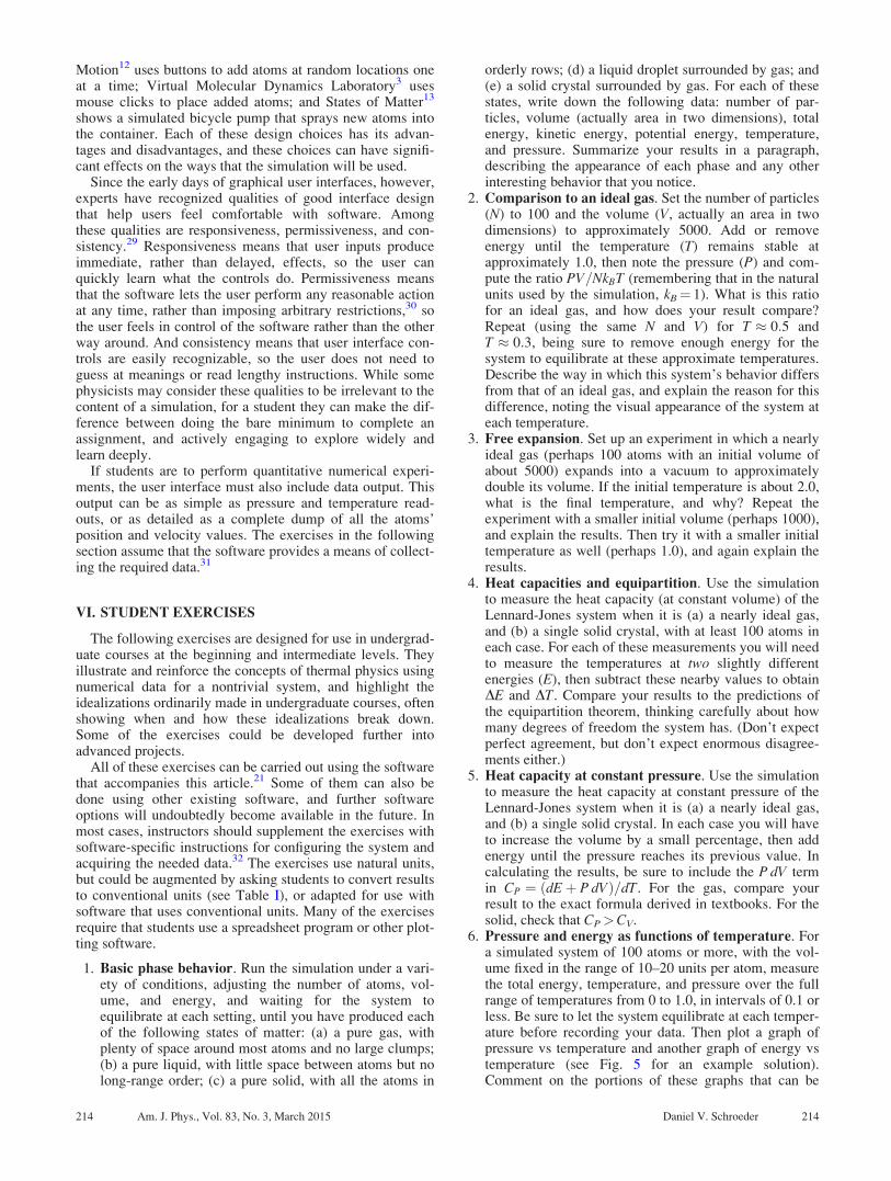
Fascinating as these equilibrium states are, however, theyare just the beginning. With suitable initialization, aLennard-Jones simulation can also show a huge variety ofnonequilibrium states and their subsequent evolution towardequilibrium. Figure 3 shows just a few of the possibilities.

Exploring the evolution of nonequilibrium states can givestudents a vivid understanding of the arrow of time.

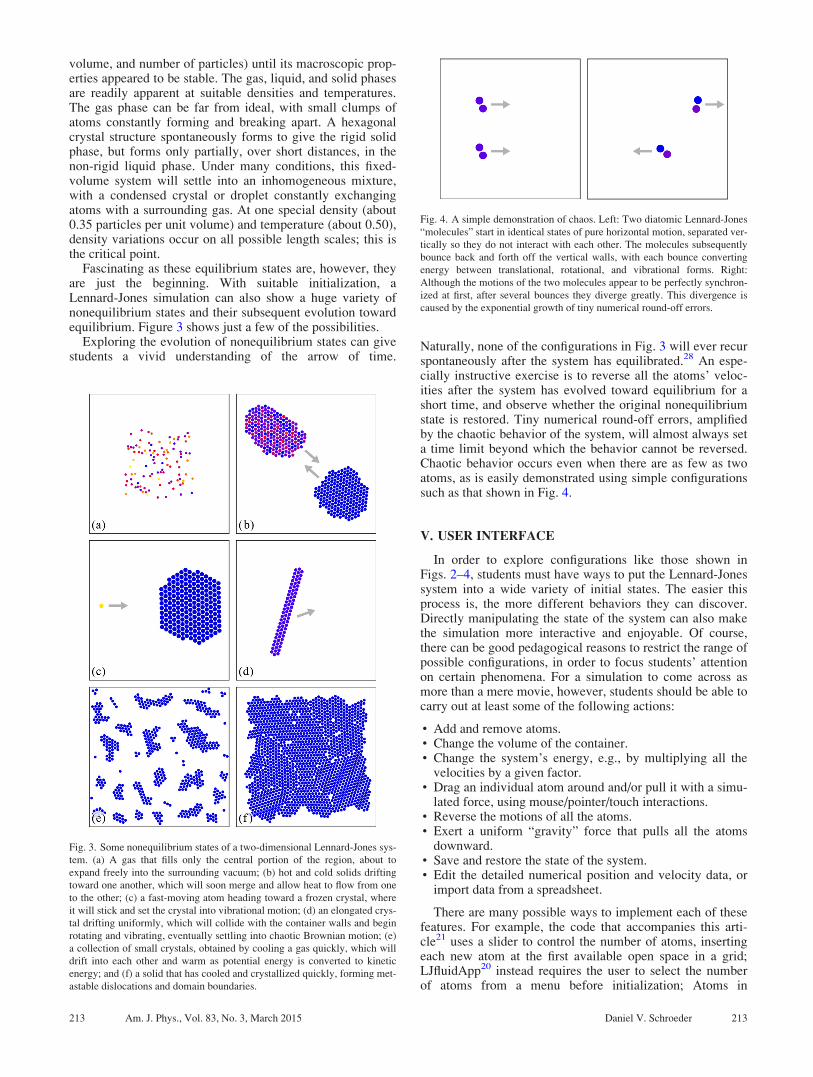
Naturally, none of the configurations in Fig. 3 will ever recurspontaneously after the system has equilibrated.28 An espe-cially instructive exercise is to reverse all the atoms’ veloc-ities after the system has evolved toward equilibrium for ashort time, and observe whether the original nonequilibriumstate is restored. Tiny numerical round-off errors, amplifiedby the chaotic behavior of the system, will almost always seta time limit beyond which the behavior cannot be reversed.Chaotic behavior occurs even when there are as few as twoatoms, as is easily demonstrated using simple configurationssuch as that shown in Fig. 4.

V. USER INTERFACE

In order to explore configurations like those shown inFigs. 2–4, students must have ways to put the Lennard-Jonessystem into a wide variety of initial states. The easier thisprocess is, the more different behaviors they can discover.Directly manipulating the state of the system can also makethe simulation more interactive and enjoyable. Of course,there can be good pedagogical reasons to restrict the range ofpossible configurations, in order to focus students’ attentionon certain phenomena. For a simulation to come across asmore than a mere movie, however, students should be able tocarry out at least some of the following actions:

• Add and remove atoms.• Change the volume of the container.• Change the system’s energy, e.g., by multiplying all the

velocities by a given factor.• Drag an individual atom around and/or pull it with a simu-

lated force, using mouse/pointer/touch interactions.• Reverse the motions of all the atoms.• Exert a uniform “gravity” force that pulls all the atoms

downward.• Save and restore the state of the system.• Edit the detailed numerical position and velocity data, or

import data from a spreadsheet.

There are many possible ways to implement each of thesefeatures. For example, the code that accompanies this arti-cle21 uses a slider to control the number of atoms, insertingeach new atom at the first available open space in a grid;LJfluidApp20 instead requires the user to select the numberof atoms from a menu before initialization; Atoms in

Fig. 3. Some nonequilibrium states of a two-dimensional Lennard-Jones sys-

tem. (a) A gas that fills only the central portion of the region, about to

expand freely into the surrounding vacuum; (b) hot and cold solids drifting

toward one another, which will soon merge and allow heat to flow from one

to the other; (c) a fast-moving atom heading toward a frozen crystal, where

it will stick and set the crystal into vibrational motion; (d) an elongated crys-

tal drifting uniformly, which will collide with the container walls and begin

rotating and vibrating, eventually settling into chaotic Brownian motion; (e)

a collection of small crystals, obtained by cooling a gas quickly, which will

drift into each other and warm as potential energy is converted to kinetic

energy; and (f) a solid that has cooled and crystallized quickly, forming met-

astable dislocations and domain boundaries.

Fig. 4. A simple demonstration of chaos. Left: Two diatomic Lennard-Jones

“molecules” start in identical states of pure horizontal motion, separated ver-

tically so they do not interact with each other. The molecules subsequently

bounce back and forth off the vertical walls, with each bounce converting

energy between translational, rotational, and vibrational forms. Right:

Although the motions of the two molecules appear to be perfectly synchron-

ized at first, after several bounces they diverge greatly. This divergence is

caused by the exponential growth of tiny numerical round-off errors.

213 Am. J. Phys., Vol. 83, No. 3, March 2015 Daniel V. Schroeder 213

Motion12 uses buttons to add atoms at random locations oneat a time; Virtual Molecular Dynamics Laboratory3 usesmouse clicks to place added atoms; and States of Matter13

shows a simulated bicycle pump that sprays new atoms intothe container. Each of these design choices has its advan-tages and disadvantages, and these choices can have signifi-cant effects on the ways that the simulation will be used.

Since the early days of graphical user interfaces, however,experts have recognized qualities of good interface designthat help users feel comfortable with software. Amongthese qualities are responsiveness, permissiveness, and con-sistency.29 Responsiveness means that user inputs produceimmediate, rather than delayed, effects, so the user canquickly learn what the controls do. Permissiveness meansthat the software lets the user perform any reasonable actionat any time, rather than imposing arbitrary restrictions,30 sothe user feels in control of the software rather than the otherway around. And consistency means that user interface con-trols are easily recognizable, so the user does not need toguess at meanings or read lengthy instructions. While somephysicists may consider these qualities to be irrelevant to thecontent of a simulation, for a student they can make the dif-ference between doing the bare minimum to complete anassignment, and actively engaging to explore widely andlearn deeply.

If students are to perform quantitative numerical experi-ments, the user interface must also include data output. Thisoutput can be as simple as pressure and temperature read-outs, or as detailed as a complete dump of all the atoms’position and velocity values. The exercises in the followingsection assume that the software provides a means of collect-ing the required data.31

VI. STUDENT EXERCISES

The following exercises are designed for use in undergrad-uate courses at the beginning and intermediate levels. Theyillustrate and reinforce the concepts of thermal physics usingnumerical data for a nontrivial system, and highlight theidealizations ordinarily made in undergraduate courses, oftenshowing when and how these idealizations break down.Some of the exercises could be developed further intoadvanced projects.

All of these exercises can be carried out using the softwarethat accompanies this article.21 Some of them can also bedone using other existing software, and further softwareoptions will undoubtedly become available in the future. Inmost cases, instructors should supplement the exercises withsoftware-specific instructions for configuring the system andacquiring the needed data.32 The exercises use natural units,but could be augmented by asking students to convert resultsto conventional units (see Table I), or adapted for use withsoftware that uses conventional units. Many of the exercisesrequire that students use a spreadsheet program or other plot-ting software.

1. Basic phase behavior. Run the simulation under a vari-ety of conditions, adjusting the number of atoms, vol-ume, and energy, and waiting for the system toequilibrate at each setting, until you have produced eachof the following states of matter: (a) a pure gas, withplenty of space around most atoms and no large clumps;(b) a pure liquid, with little space between atoms but nolong-range order; (c) a pure solid, with all the atoms in

orderly rows; (d) a liquid droplet surrounded by gas; and(e) a solid crystal surrounded by gas. For each of thesestates, write down the following data: number of par-ticles, volume (actually area in two dimensions), totalenergy, kinetic energy, potential energy, temperature,and pressure. Summarize your results in a paragraph,describing the appearance of each phase and any otherinteresting behavior that you notice.

2. Comparison to an ideal gas. Set the number of particles(N) to 100 and the volume (V, actually an area in twodimensions) to approximately 5000. Add or removeenergy until the temperature (T) remains stable atapproximately 1.0, then note the pressure (P) and com-pute the ratio PV=NkBT (remembering that in the naturalunits used by the simulation, kB¼ 1). What is this ratiofor an ideal gas, and how does your result compare?Repeat (using the same N and V) for T � 0:5 andT � 0:3, being sure to remove enough energy for thesystem to equilibrate at these approximate temperatures.Describe the way in which this system’s behavior differsfrom that of an ideal gas, and explain the reason for thisdifference, noting the visual appearance of the system ateach temperature.

3. Free expansion. Set up an experiment in which a nearlyideal gas (perhaps 100 atoms with an initial volume ofabout 5000) expands into a vacuum to approximatelydouble its volume. If the initial temperature is about 2.0,what is the final temperature, and why? Repeat theexperiment with a smaller initial volume (perhaps 1000),and explain the results. Then try it with a smaller initialtemperature as well (perhaps 1.0), and again explain theresults.

4. Heat capacities and equipartition. Use the simulationto measure the heat capacity (at constant volume) of theLennard-Jones system when it is (a) a nearly ideal gas,and (b) a single solid crystal, with at least 100 atoms ineach case. For each of these measurements you will needto measure the temperatures at two slightly differentenergies (E), then subtract these nearby values to obtainDE and DT. Compare your results to the predictions ofthe equipartition theorem, thinking carefully about howmany degrees of freedom the system has. (Don’t expectperfect agreement, but don’t expect enormous disagree-ments either.)

5. Heat capacity at constant pressure. Use the simulationto measure the heat capacity at constant pressure of theLennard-Jones system when it is (a) a nearly ideal gas,and (b) a single solid crystal. In each case you will haveto increase the volume by a small percentage, then addenergy until the pressure reaches its previous value. Incalculating the results, be sure to include the P dV termin CP ¼ ðdEþ P dVÞ=dT. For the gas, compare yourresult to the exact formula derived in textbooks. For thesolid, check that CP>CV.

6. Pressure and energy as functions of temperature. Fora simulated system of 100 atoms or more, with the vol-ume fixed in the range of 10–20 units per atom, measurethe total energy, temperature, and pressure over the fullrange of temperatures from 0 to 1.0, in intervals of 0.1 orless. Be sure to let the system equilibrate at each temper-ature before recording your data. Then plot a graph ofpressure vs temperature and another graph of energy vstemperature (see Fig. 5 for an example solution).Comment on the portions of these graphs that can be

214 Am. J. Phys., Vol. 83, No. 3, March 2015 Daniel V. Schroeder 214

understood in terms of the ideal gas law and the equipar-tition theorem, and on the portions that cannot be sosimply understood (and why). How does the low-temperature behavior of the heat capacity differ fromthat of a real-world solid?

7. Heat capacity and entropy. From your data in the pre-vious problem, construct a graph of the heat capacity atconstant volume, CV , as a function of temperature. Youmay have to do some smoothing to reduce the effects ofnoise in the data. Then construct a table and graph ofCV=T vs T, and numerically integrate this function (to anaccuracy of one or two significant figures) to determinethe entropy as a function of temperature, relative to theentropy at T¼ 0.1. Why can’t you determine the abso-lute entropy, relative to T¼ 0? Why doesn’t this limita-tion affect real-world materials?

8. Critical point. Set the number of atoms to at least 1000(more is better) and the volume, in natural units, toapproximately three times the number of atoms. Addand remove energy to carefully explore the behavior ofthe system over the temperature range from about 0.4 to0.7, and describe how its appearance changes over thisrange. What is your best estimate of the critical tempera-ture of this system, and what is the correspondingpressure?

9. Phase diagram. Map out the approximate phase dia-gram of the two-dimensional Lennard-Jones system, byadjusting both the temperature and the volume to findthe various phase boundary lines (where two phasescoexist in equilibrium). Keep the number of atoms fixed

(preferably at 500 or more). It’s easiest to start at a largevolume and low temperature, so the system consists of asingle solid crystal surrounded by a low-density gas.Add energy gradually, letting the system equilibrate atvarious temperatures and noting the temperature andpressure after each equilibration. Be sure to note the ap-proximate triple point, where the solid crystal (withatoms in orderly rows) melts into a liquid (with no long-range order). The critical point is the subject of the pre-vious problem. Finally, reduce the volume (and theenergy) to try to locate the solid-liquid phase boundaryat pressures somewhat above that of the triple point. Plotall of your pressure-temperature measurements, sketch-ing in the approximate phase boundary lines and anno-tating the plot with descriptions of the system’sappearance under the various conditions.

10. Phase boundary ambiguities. Phase boundary lines aresharp (because the properties of the system across aboundary are discontinuous) only in the limit of an infin-itely large system. As a follow-up to the previous prob-lem, explore how the phase boundary locations dependon the volume of the system and on the number ofatoms. For example, try plotting the liquid-gas phaseboundary for systems with different sizes but similar av-erage densities. Explain the results qualitatively, by con-sidering what fraction of the atoms in the liquid dropletare near the surface.

11. Velocity distribution. Record the instantaneous veloc-ities (x and y components) for 1000 or more atoms inequilibrium at a temperature of about 0.5 in naturalunits. Using a spreadsheet or other software, plot a histo-gram of the vx values, using about 20 bins to cover thevelocity interval �2.0 toþ 2.0. Do the same for the vy

values. Also plot the expected results according to theMaxwell-Boltzmann velocity distribution, which for

either component vi isffiffiffiffiffiffiffiffiffiffiffiffiffiffiffiffiffiffiffiffiffiffim=ð2pkBTÞ

pexpð�mv2

i =2kBTÞ.(This is the function that, when multiplied by any smallvelocity interval dvi, gives the probability of finding asingle atom within this interval. To compare it to yoursimulation results, you will have to take into account thenumber of atoms and the sizes of the histogram bins.)Repeat this whole procedure for a different temperature(adjusting the histogram range if necessary) and discussthe results. Does it matter whether the simulated materialis in a solid, liquid, or gas state?

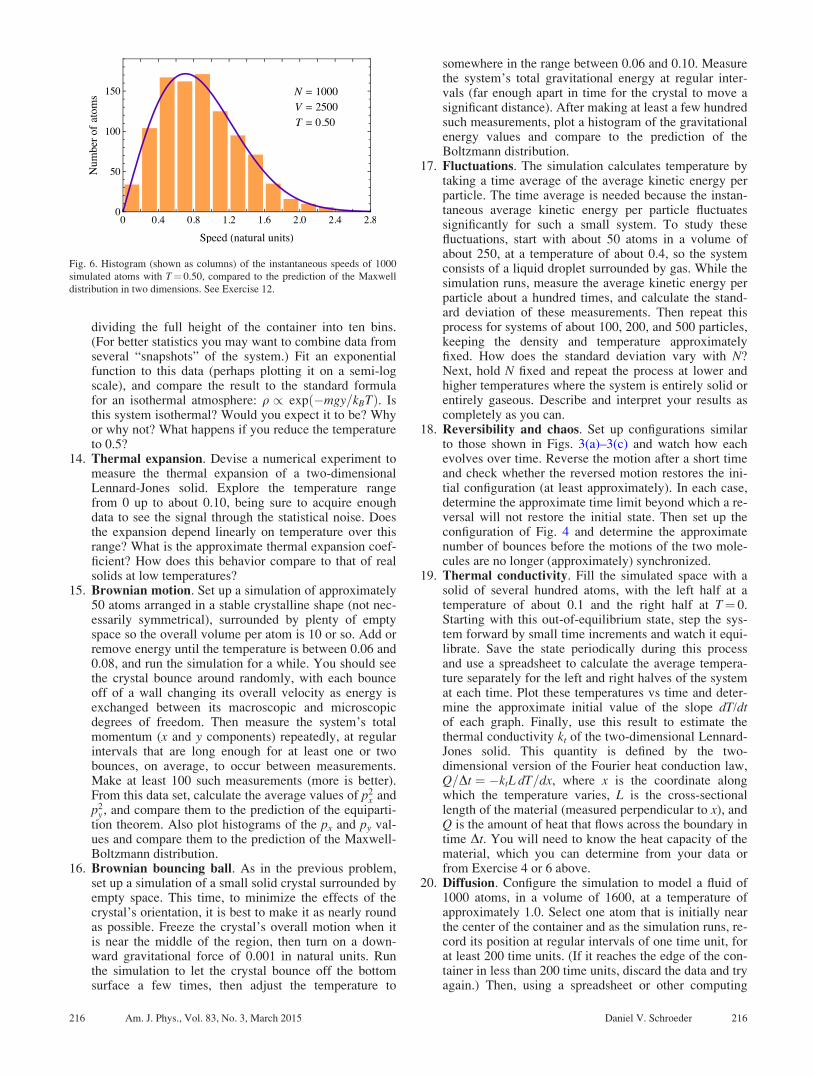
12. Speed distribution. As in the previous problem, recordthe instantaneous velocity components of 1000 or moreatoms in equilibrium. Use a spreadsheet to calculate thespeed of each atom, plot a histogram of the speeds, andcompare to the theoretical prediction (i.e., the two-dimensional Maxwell speed distribution). (See Fig. 6 foran example solution.) Why does the speed distributionequal zero at v¼ 0, whereas the distributions for vx andvy have their peaks at vx¼ 0 and vy¼ 0?

13. Gas density in a gravitational field. Set the size of thecontainer to 100� 100, the number of atoms to 500, thegravitational constant to 0.02, and the temperature toabout 1.0. The system is now an “atmosphere” whosedensity decreases with altitude. How does the typicalgravitational energy compare to the typical kineticenergy? Record the positions of all the atoms at oneinstant and use a spreadsheet (or other software) to plot agraph of relative density (q) as a function of altitude,

Fig. 5. Pressure (top) and energy per particle (bottom) as functions of tem-

perature for a simulated system of 100 Lennard-Jones particles in a two-

dimensional volume of 1600. All quantities are in natural units. The straight

lines show the ideal gas pressure NkBT=V and the equipartition predictions

for the heat capacities C of a solid (C=N ¼ 4ð1=2ÞkB) and an ideal gas

(C=N ¼ 2ð1=2ÞkB). See Exercise 6.

215 Am. J. Phys., Vol. 83, No. 3, March 2015 Daniel V. Schroeder 215

dividing the full height of the container into ten bins.(For better statistics you may want to combine data fromseveral “snapshots” of the system.) Fit an exponentialfunction to this data (perhaps plotting it on a semi-logscale), and compare the result to the standard formulafor an isothermal atmosphere: q / expð�mgy=kBTÞ. Isthis system isothermal? Would you expect it to be? Whyor why not? What happens if you reduce the temperatureto 0.5?

14. Thermal expansion. Devise a numerical experiment tomeasure the thermal expansion of a two-dimensionalLennard-Jones solid. Explore the temperature rangefrom 0 up to about 0.10, being sure to acquire enoughdata to see the signal through the statistical noise. Doesthe expansion depend linearly on temperature over thisrange? What is the approximate thermal expansion coef-ficient? How does this behavior compare to that of realsolids at low temperatures?

15. Brownian motion. Set up a simulation of approximately50 atoms arranged in a stable crystalline shape (not nec-essarily symmetrical), surrounded by plenty of emptyspace so the overall volume per atom is 10 or so. Add orremove energy until the temperature is between 0.06 and0.08, and run the simulation for a while. You should seethe crystal bounce around randomly, with each bounceoff of a wall changing its overall velocity as energy isexchanged between its macroscopic and microscopicdegrees of freedom. Then measure the system’s totalmomentum (x and y components) repeatedly, at regularintervals that are long enough for at least one or twobounces, on average, to occur between measurements.Make at least 100 such measurements (more is better).From this data set, calculate the average values of p2

x andp2

y , and compare them to the prediction of the equiparti-tion theorem. Also plot histograms of the px and py val-ues and compare them to the prediction of the Maxwell-Boltzmann distribution.

16. Brownian bouncing ball. As in the previous problem,set up a simulation of a small solid crystal surrounded byempty space. This time, to minimize the effects of thecrystal’s orientation, it is best to make it as nearly roundas possible. Freeze the crystal’s overall motion when itis near the middle of the region, then turn on a down-ward gravitational force of 0.001 in natural units. Runthe simulation to let the crystal bounce off the bottomsurface a few times, then adjust the temperature to

somewhere in the range between 0.06 and 0.10. Measurethe system’s total gravitational energy at regular inter-vals (far enough apart in time for the crystal to move asignificant distance). After making at least a few hundredsuch measurements, plot a histogram of the gravitationalenergy values and compare to the prediction of theBoltzmann distribution.

17. Fluctuations. The simulation calculates temperature bytaking a time average of the average kinetic energy perparticle. The time average is needed because the instan-taneous average kinetic energy per particle fluctuatessignificantly for such a small system. To study thesefluctuations, start with about 50 atoms in a volume ofabout 250, at a temperature of about 0.4, so the systemconsists of a liquid droplet surrounded by gas. While thesimulation runs, measure the average kinetic energy perparticle about a hundred times, and calculate the stand-ard deviation of these measurements. Then repeat thisprocess for systems of about 100, 200, and 500 particles,keeping the density and temperature approximatelyfixed. How does the standard deviation vary with N?Next, hold N fixed and repeat the process at lower andhigher temperatures where the system is entirely solid orentirely gaseous. Describe and interpret your results ascompletely as you can.

18. Reversibility and chaos. Set up configurations similarto those shown in Figs. 3(a)–3(c) and watch how eachevolves over time. Reverse the motion after a short timeand check whether the reversed motion restores the ini-tial configuration (at least approximately). In each case,determine the approximate time limit beyond which a re-versal will not restore the initial state. Then set up theconfiguration of Fig. 4 and determine the approximatenumber of bounces before the motions of the two mole-cules are no longer (approximately) synchronized.

19. Thermal conductivity. Fill the simulated space with asolid of several hundred atoms, with the left half at atemperature of about 0.1 and the right half at T¼ 0.Starting with this out-of-equilibrium state, step the sys-tem forward by small time increments and watch it equi-librate. Save the state periodically during this processand use a spreadsheet to calculate the average tempera-ture separately for the left and right halves of the systemat each time. Plot these temperatures vs time and deter-mine the approximate initial value of the slope dT/dtof each graph. Finally, use this result to estimate thethermal conductivity kt of the two-dimensional Lennard-Jones solid. This quantity is defined by the two-dimensional version of the Fourier heat conduction law,Q=Dt ¼ �ktL dT=dx, where x is the coordinate alongwhich the temperature varies, L is the cross-sectionallength of the material (measured perpendicular to x), andQ is the amount of heat that flows across the boundary intime Dt. You will need to know the heat capacity of thematerial, which you can determine from your data orfrom Exercise 4 or 6 above.

20. Diffusion. Configure the simulation to model a fluid of1000 atoms, in a volume of 1600, at a temperature ofapproximately 1.0. Select one atom that is initially nearthe center of the container and as the simulation runs, re-cord its position at regular intervals of one time unit, forat least 200 time units. (If it reaches the edge of the con-tainer in less than 200 time units, discard the data and tryagain.) Then, using a spreadsheet or other computing

Fig. 6. Histogram (shown as columns) of the instantaneous speeds of 1000

simulated atoms with T¼ 0.50, compared to the prediction of the Maxwell

distribution in two dimensions. See Exercise 12.

216 Am. J. Phys., Vol. 83, No. 3, March 2015 Daniel V. Schroeder 216

environment, compute the squared displacement,ðDxÞ2 þ ðDyÞ2, for each of the (200 or so) one-unit timeintervals in your data set. Average these values to obtainthe mean squared displacement (MSD). Similarly, usethe same data set to calculate the MSD for time intervals(Dt) of 2, 5, 10, and 20 units. Plot the MSD vs Dt andnotice that the graph is approximately linear; this is thecharacteristic behavior of diffusive motion (or a so-called random walk). The slope of the line is closelyrelated to the diffusion constant D; in two dimensions,the MSD is 4DDt. Estimate the diffusion constant fromyour data, then repeat the analysis, holding the fluid den-sity fixed, at temperatures of approximately 0.5 and 2.0.

VII. ENHANCEMENTS

As the preceding sections illustrate, the pure Lennard-Jones system exhibits a rich variety of physical behaviorsthat can keep students occupied almost indefinitely. Still,there are sometimes good reasons to go beyond the pureLennard-Jones system.

Atoms in Motion,12 for example, can simulate arbitrarymixtures of Lennard-Jones particles of five different types,with sizes, masses, and interaction strengths chosen to modelhelium, neon, argon, krypton, and xenon. States of Matter13

cannot simulate mixtures, but can separately simulate four dif-ferent types of molecules: two different noble gases, a rigiddiatomic species (“oxygen”), and a rigid triatomic species(“water”). Molecular Workbench14 includes an option formodeling charged ions that exert long-range Coulomb forces.

In the spirit of encouraging interactive exploration, thesoftware accompanying this article21 allows the user to con-nect any two atoms together with an elastic “bond” that addsa spring-like force to the Lennard-Jones force. This feature isquite versatile and was easy to code. It is not an accuratemodel of actual covalent bonds, because there is no limit onthe number of bonds per atom, there are no constraints onthe angles between bonds, and the bond stiffness, for compu-tational reasons, is unrealistically low. Still, even this crudemodel of bonds enables some interesting demonstrations andexperiments, such as measuring the heat capacity of a dia-tomic gas (including the contribution of vibrational potentialenergy), watching the Brownian motion of a large objectbombarded by fast-moving atoms, and observing the frictionof one solid object sliding over another (see Fig. 7).

The same simulation also incorporates a second ad hocfeature: the ability to anchor an atom so that it is fixed inspace. In this way the user can build barriers and even simu-late nano-scale “machinery” such as a version of the famousBrownian ratchet.33 If nothing else, such demonstrations viv-idly illustrate how the nano-scale world, with its van derWaals forces and perpetual jiggling motions, differs from themacroscopic world we are used to.

VIII. DISCUSSION

In summary, an interactive molecular dynamics simulationcan augment the teaching of thermal physics and relatedtopics in a variety of ways, complementing the more tradi-tional approaches and highlighting some of the idealizationsthat those approaches require.

On the other hand, any computer simulation incorporatesits own set of idealizations and limitations. The simulations

described in this article are limited to a rather small numberof particles (no more than a few thousand), living in a two-dimensional world. These simulations are reasonably accu-rate at modeling only noble gas atoms, and make no attemptto model chemical reactions.

A critical yet intrinsic limitation is that these simulationsdo not incorporate any quantum effects. This limitationmeans that their low-temperature behavior is never realistic,because quantum effects are responsible for the “freezingout” of degrees of freedom and other phenomena related tothe third law of thermodynamics. Other approaches34 can beused to introduce students to thermodynamic systems at lowtemperature, at least when the systems are in equilibrium.

No “canned” simulation can offer students the sameopportunities for open-ended exploration as writing theirown code. It is my hope that, after a certain amount of timespent with the interactive simulations described here—andreaching the limits of what their graphical user interfacesallow—students will be motivated to take the next step andbegin modifying the code, or writing their own, to conductfurther explorations.

Finally, we should remember that no simulation or numer-ical “experiment” is a substitute for carrying out real experi-ments on real physical systems. Rather, a simulation canhelp bridge the gap between theory and experiment, and of-ten, for thermodynamic systems, between the microscopicand the macroscopic.

Fig. 7. A few of the configurations that are possible with a molecular dy-

namics simulation that allows connecting atoms together with “bonds” and

anchoring atoms at fixed locations.

217 Am. J. Phys., Vol. 83, No. 3, March 2015 Daniel V. Schroeder 217

ACKNOWLEDGMENTS

The author is grateful to Adam Johnston, JohnMallinckrodt, Tom Moore, and Paul Weber for theirassistance and suggestions regarding various aspects of thisarticle. This work was supported in many ways by WeberState University.

a)Electronic mail: dschroeder@weber.edu1R. P. Feynman, R. B. Leighton, and M. Sands, The Feynman Lectures onPhysics (Addison-Wesley, Reading, MA, 1963), Vol. I, available online at

<http://www.feynmanlectures.caltech.edu/>. The “atomic hypothesis”

quote is on p. 1-2.2For a video interview of Feynman applying his imagination and thinking

to the atomic hypothesis, see “Fun to Imagine I: Jiggling Atoms,” BBC

program first broadcast July 8, 1983, <http://www.bbc.co.uk/archive/feyn-

man/10700.shtml>, also available at <https://www.youtube.com/

watch?v¼v3pYRn5j7oI>.3Boston University Center for Polymer Studies, “Virtual Molecular

Dynamics Laboratory,” <http://polymer.bu.edu/vmdl/>. This Web site

also introduces molecular dynamics with the Feynman “atomic hypoth-

esis” quote, which is too good not to steal.4S. Novick and J. Nussbaum, “Pupils’ understanding of the particulate na-

ture of matter: A cross-age study,” Sci. Educ. 65(2), 187–196 (1981).5R. Driver et al., Making Sense of Secondary Science: Research intoChildren’s Ideas (Routledge, London, 1994), Chap. 11.

6A. B. Arons, A Guide to Introductory Physics Teaching (Wiley, New

York, 1990), pp. 274–281.7M. P. Allen and D. J. Tildesley, Computer Simulation of Liquids(Clarendon Press, Oxford, 1987).

8J. M. Haile, Molecular Dynamics Simulation (Wiley, New York, 1992).9D. C. Rapaport, The Art of Molecular Dynamics Simulation, 2nd ed.

(Cambridge U.P., Cambridge, 2004).10Stark Design, “Atomic Microscope” (Windows and Mac Classic applica-

tion). This software, first released around 1999, is apparently no longer

available, but is described in Ref. 11 and is similar in many ways to Atoms

in Motion, Ref. 12.11S. Carlson, “Modeling the atomic universe,” Sci. Am. 281(4), 118–119

(1999).12Atoms in Motion LLC, “Atoms in Motion” (iPad app), <http://www.atom-

sinmotion.com/> (2011–2012).13PhET project, “States of Matter” (JAVA Web Start application), <http://

phet.colorado.edu/en/simulation/states-of-matter> (2009–2012).14The Concord Consortium, “Molecular Workbench” (JAVA simulations and

modeling tools), <http://mw.concord.org/> (2004–2013). A new HTML5

version is also available, at <http://mw.concord.org/nextgen/>.15H. Gould, J. Tobochnik, and W. Christian, An Introduction to Computer

Simulation Methods, 3rd ed. (Pearson Addison Wesley, San Francisco, 2007).16N. J. Giordano and H. Nakanishi, Computational Physics, 2nd ed.

(Pearson Prentice Hall, Upper Saddle River, NJ, 2006).17D. V. Schroeder, Physics Simulations in JAVA: A Lab Manual (unpublished)

2006–2011, <http://physics.weber.edu/schroeder/javacourse/>.18L. M. Sander, Equilibrium Statistical Physics: With Computer Simulations

in Python (CreateSpace Independent Publishing, Seattle, 2013), URL:

<http://www-personal.umich.edu/~lsander/ESP/ESP.htm>.19H. Gould and J. Tobochnik, Statistical and Thermal Physics: With

Computer Applications (Princeton U.P., Princeton, 2010).20Open Source Physics Project, “LJfluidApp,” <http://stp.clarku.edu/simula-

tions/lj/md/index.html> (2009).21See supplemental material at http://dx.doi.org/10.1119/1.4901185 for the sim-

ulation program, user instructions, and a version of the exercises in Sec. VI

that is customized for this particular simulation. These materials are also

available at<http://physics.weber.edu/schroeder/md/InteractiveMD.html>.22In this case, the van der Waals force is also called the London dispersion

force; it is caused by quantum fluctuations of the molecules’ electronic

charge distributions. The 1=r6 dependence is derived using perturbation

theory in many quantum mechanics textbooks. See also B. R. Holstein,

“The van der Waals interaction,” Am. J. Phys. 69(4), 441–449 (2001); and

K. A. Milton, “Resource Letter VWCPF-1: van der Waals and Casimir-

Polder forces,” Am. J. Phys. 79(7), 697–711 (2011).23G. C. Maitland et al., Intermolecular Forces: Their Origin and

Determination (Clarendon Press, Oxford, 1981). This monograph makes

an exhaustive assessment of the limitations of the Lennard-Jones 6-12

potential.24The walls can be hard, producing instantaneous reversals in velocity, or

soft, exerting a spring-like repulsive force that grows as atoms penetrate

into the walls more deeply. The accompanying code (Ref. 21) uses soft

walls (with a spring constant of 50 in natural units), because of the sim-

plicity of all forces being smoothly varying functions of position. A disad-

vantage of this method is that the volume of the simulated space is

somewhat variable and hence ambiguous, especially at high temperatures.25As of this writing, the current versions of all major browsers for personal

computers deliver impressive JAVASCRIPT performance that is more than

adequate for the simulations described in this article. Performance of

JAVASCRIPT on mobile devices, however, is much more variable.26Another popular interpreted language is PYTHON, which offers advantages in

a computational physics course or other setting where students will be writ-

ing or modifying the code. As of this writing, PYTHON’s relatively poor per-

formance limits the size of an interactive molecular dynamics simulation

running at a reasonable animation rate. However, through use of the NumPy

library (<www.numpy.org>) to vectorize the calculations (see, e.g., the

program simplemd.py in Ref. 18), one can still reach a performance level

that is adequate for most of the examples and exercises in this article.27The most powerful optimization technique is to divide the simulation

space into a grid of “cells” whose widths are no smaller than the cutoff dis-

tance. Then each atom can interact only with atoms in its own cell and the

eight nearest neighbor cells. The algorithm is described in Refs. 7 and 9

and is used in the code of Ref. 21. The additional coding can be done in

only a few dozen lines and is well worth the trouble for simulations of 500

or more particles, but provides no benefit at all when N�100.28The configuration shown in Fig. 3(f) will not spontaneously equilibrate,

but it can be annealed by gradually adding energy.29Apple Computer, Inc., Inside Macintosh (Addison-Wesley, Reading, MA,

1985), p. I-27.30Implementing “permissiveness” in a molecular dynamics simulation can

be challenging, because some potential user actions (e.g., placing the

atoms so they overlap) can add large amounts of energy to the system, trig-

gering the numerical instability described in Sec. III. The accompanying

simulation (Ref. 21) tries to adapt to dangerous user actions by decreasing

the time step dt and limiting the rate at which particles can be manually

pushed together. Still, it is not hard for a curious user to “break” the simu-

lation, generating an error message and necessitating a reset. This experi-

ence can sometimes be instructive but is usually just frustrating.31Some molecular dynamics software (Refs. 3 and 20) goes further to

include built-in plotting of various data. This feature can be useful for

quick demonstrations, but it usually reduces the degree to which the stu-

dent is actively engaged in deciding how to gather and analyze the data.

Also, as a practical matter, it is difficult to pre-program all of the different

types of plots that students and instructors might wish to make.32The online supplement (Ref. 21) to this article includes a version of the

exercises with instructions and hints that are specific to the accompanying

software.33Feynman et al., Ref. 1, Chap. 46. See also H. S. Leff and A. F. Rex,

Maxwell’s Demon 2: Entropy, Classical and Quantum Information,Computing (Institute of Physics Publishing, Bristol, 2003), Sec. 1.2.5, and

references therein.34Besides the usual approaches to quantum statistical mechanics found in

every textbook, see (for example) T. A. Moore and D. V. Schroeder, “A

different approach to introducing statistical mechanics,” Am. J. Phys.

65(1), 26–36 (1997); M. Ligare, “Numerical analysis of Bose-Einstein

condensation in a three-dimensional harmonic oscillator potential,” Am. J.

Phys. 66(3), 185–190 (1998); and J. Arnaud et al., “Illustration of the

Fermi-Dirac statistics,” Am. J. Phys. 67(3), 215–221 (1999).

218 Am. J. Phys., Vol. 83, No. 3, March 2015 Daniel V. Schroeder 218