Embed Size (px)
Citation preview

INTEREST RATE PASS-THROUGH IN COLOMBIA: A MICRO-BANKING PERSPECTIVE*
Rocío Betancourt Hernando Vargas
Norberto Rodríguez**
Bogotá, September 2006
_________________________ *The opinions expressed in this paper are those of the authors and do not represent the views of the Banco de la República or of its Board of Directors. **Assistant to the Deputy Governor, Deputy Governor and Econometrician of the Macro Modelling Department of Banco de la República, respectively. Corresponding author: Rocío Betancourt, E-mail: [email protected].

1
INTEREST RATE PASS-THROUGH IN COLOMBIA: A MICRO-BANKING PERSPECTIVE
Abstract
Banks and other credit institutions are key players in the transmission of monetary policy, especially in emerging market economies, where the responses of deposit and loan interest rates to shifts in policy rates are among the most important channels. This pass-through depends on the conditions prevailing in the loan and deposit markets, which are, in turn, affected by macroeconomic factors. Hence, when setting their policy, monetary authorities must take into account those conditions and the behavior of banks. This paper illustrates this point by means of a theoretical micro-banking model and shows empirical evidence for Colombia suggesting that some aspects of the model might be relevant features of the transmission mechanism. Keywords: Monetary Transmission Mechanisms, Interest Rate Pass-Through, Banking JEL Classification: G21, E43, E44, E52

2
1. Introduction In some economies banks and other financial institutions play a key role in the expenditure decisions of firms and households. They are among the most important alternatives of funding and means of saving. As such, banks and bank behavior are critical components of the transmission mechanism of monetary policy. In particular, the interest rate channel of monetary policy, which operates when banks transmit the changes in the monetary policy rate to their customers’ interest rates, depends on the banks’ reaction to different shocks and to the state of the economy. Hence, when setting their policy, monetary authorities should take into account banks’ behavior under different economic conditions. This paper illustrates the idea that the response of market interest rates to changes in the policy interest rate depends on the reaction of banks and financial markets to different shocks hitting the economy. For that purpose, a theoretical microeconomic model of the banking firm and the credit and deposits markets is used. We also present some evidence for the Colombian economy. The paper is organized as follows. A brief review of the literature is given in section 2. A discussion about the importance of the banking system and interest rate pass-through in Colombia is presented in section 3. A theoretical model of the banking firm and the financial markets equilibrium is developed in section 4. This model includes the effects of monetary policy and other macroeconomic conditions. The model is then used to interpret some episodes of interest rate transmission in Colombia. In section 5, some econometric evidence is shown. Finally, in section 6 we discuss the importance for the Central Bank to understand the role of banks’ and financial markets’ behavior in the interest rate pass-through. We do so by means of numerical simulations of a small-open economy macro model which includes a simple version of our micro-banking model. 2. Literature Review The literature has identified different transmission mechanisms of monetary policy such as the interest rate channel, the credit channel and the exchange rate channel among others1. The importance of the banking sector in the transmission of interest rates has been recently recognized in the literature on the interest rate channel2. At the same time, the credit channel has focused on the agency problems that arise between financial institutions, particularly banks, and the agents to which they lend (Bernanke and Gertler, 1995) 3. Therefore, the credit channel is now considered as a set of factors that amplify and propagate the effects of the interest rate channel through their impact on lending rates and other interest rate spreads.
1 See Loayza and Schmidt-Hebbel (2002) for an overview about the transmission mechanisms. 2 The importance of the banking sector in the interest rate pass-through is theoretically studied by Hannan and Berger (1991) and empirically assessed by Cottarelli and Kourelis (1994). For an overview of the banking industry and monetary policy literature see Ahumada and Fuentes (2004). 3 In contrast to the classical monetarist view that emphasizes the role of narrow and broad monetary aggregates in determining prices.
3
The banking sector has been incorporated in this literature, focusing mainly on the financial structure and information asymmetries4. These two elements clearly influence the behavior of banks and help explain why lending and deposit rates may show a limited response to changes in the monetary policy rate. From Hannan and Berger (1991) and Cottarelli and Kourelis (1994), the stickiness of bank lending interest rates after a change in the money market rates has been explained by different features of the financial structure. Empirical studies, like Berstein and Fuentes (2003) and Kot (2004) have found some degree of rigidity of interest rates in the short run and higher long-run interest rate pass-through coefficients. The degree of competition in the banking sector, the size of the bank, the types of customers and the loan risk level, among other financial features, have been found as the main determinants of interest rate flexibility5. Furthermore, depending on the country and also on the maturity of the interest rates, they may respond less than one-for-one to policy rates, so that the pass-through is incomplete at least in the short run (e.g. De Bondt, 2005). The macroeconomic implications of an incomplete long-run pass-through from policy to bank interest rates are analyzed by Kwapil and Scharler (2005), who found that, under these conditions, the Taylor Principle can be insufficient for equilibrium determinacy6. On a wider perspective, financial structure may influence interest rate pass-through by affecting the response of the financial markets to macroeconomic conditions. In particular, a macroeconomic shock may impact market interest rates directly and in addition to the response of the policy rate to the shock. In this sense, not only market rates may react with a delay to movements in policy rates, but also they may react more, less, or simply not react at all in the short run. As a result, the estimation of interest rate pass-through must control for the direct impact of other macro variables on market rates. This paper presents the latter ideas in some detail and explores the evidence of their relevance in the Colombian data. 3. The Transmission of the Interest Rates in Colombia Studies for Colombia have found that, although there is a long-term relationship between policy and bank interest rates, interest rate pass-through is incomplete. Some of these studies have also documented the importance of the banking sector in Colombia and have suggested its significance in the transmission of interest rates.
4 Cottarelli and Kourelis (1994) consider the financial structure as a term that broadly includes different features such as the degree of development of financial markets, the degree of competition within the banking system, the existence of constraints on capital movements and the ownership structure of the financial intermediaries. 5 According to Cottarelli and Kourelis (1994) interest rate stickiness means that in the presence of a change of money market rates, bank rates change by a smaller amount in the short run (short-run stickiness) and possibly also in the long run (long-run stickiness). 6 This principle states that nominal interest rates have to respond at least one-for-one to changes in the expected inflation rate to guarantee a stable and unique equilibrium.

4
Julio (2001) found a stable long-term relationship between the interest rates in Colombia using cointegration for two periods, before and after the removal of the exchange rate band. Huertas et al. (2005) used descriptive statistics7 to estimate that a 1% change in the monetary policy rate implies a change of 0.26% in the 90-day CDs rate in the short-run and a change of 0.6% in the long run8. In addition, using VAR models they found that commercial short term, lending rates react one-for-one to the deposit rate, while the short-run pass-through is just 42% for the ‘preferential’ short term, lending rate. Huertas et al. (2005) show that bank credit was the most important source of funds for firms between 2000 and 20049. However they suggest that the rather low transmission of the monetary policy interest rate to market interest rates can be explained by a loss in the effectiveness of the credit channel. They attributed this to the increase of banks’ holdings of Government bonds as an alternative to loans10, and to the declining share of bank loans as a source of funds for firms during the period (2000-2004). This is in agreement with the results of Zamudio and Martinez (2006), who found that firms decreased their debt with the financial sector in 2005 and internal savings were their main source of funds (52% in contrast to 48% of external resources)11. These results show that the importance of substitutes for loans in banks’ and firms’ balance sheets has increased. However, this change may reflect the adjustment made by agents after the financial crisis and the recession of 1998-1999, and not necessarily a structural change. A reduction of the loan supply might have been due to the higher risk perception of the economy by the financial system after the crisis, and a decrease in loan demand could have occurred because of an explicit policy of leverage reduction by firms and households. Bank loans and deposits remain an important component of private sector liabilities and assets, according to the flow of funds accounts. Financial debt funded on average 42% of the households’ and small firms’ total assets during the period 1996-2004. This figure is 18% for financial-statement-reporting firms in the same period. This proportion fell after the recession, but has recovered in recent years (Graph 1). Further, the proportion of small firms’ and households’ assets held as deposits in the financial system was on average 42% of their total assets for the same period12. This evidence suggests that the banking sector plays a relevant role as a provider of funds and as a deposit system for the private sector in the Colombian economy13. Hence, a
7 The authors also use VAR models in differences in order to see the impact of the interbank interest rate on the 90-day CDs interest rate (DTF). 8 The short run corresponds to one week and the long-run elasticity was calculated as an average of the change in the interest rates between movements in policy rates during the period from March 2001 to December 2004. 9 The authors analyzed a sample of 3.585 financial-statement-reporting firms. 10 According to the authors the proportion of the private credit on the banks’ total assets was 85% in 1994 and 65% in 2004, while the banks’ public investments as a proportion of the total assets increased from 7% to 27% during the same period. 11 The sample analyzed includes 18.588 firms that reported their financial statements during 2005. 12 This proportion is 50% if pensions are not taken into account. 13 According to Villar, L. et al. (2005), in 2001 the domestic private credit/GDP ratio (a measure of financial deepening) was 25% for Colombia, similar to the ratios for Argentina, Perú and Ecuador. This indicator was 65% for Chile, 97% for Thailand, 125% for China and 150% for Malaysia.

5
complete analysis of the monetary transmission channels and interest rate pass-through must take into account bank behavior and the equilibrium in the loan and deposit markets.
Graph 1.
0%
10%
20%
30%
40%
50%
60%
1996 1997 1998 1999 2000 2001 2002 2003 2004
Private Sector Financial Debt/ Total Assets
Firms Households
Source: Banco de la República
4. A Micro-Banking Model Recently, microeconomic models of banks’ behavior have been used to explain the role of financial structure in the transmission of interest rates. Berstein and Fuentes (2003) present a Monti-Klein model to explain the long run behavior of the banks under imperfect competition, taking into account the existence of credit risk. By using disaggregated data for different banks, they find that banks’ characteristics other than the industrial organization can influence the degree of delay in the market interest rate response to changes in the policy rate. Kot (2004) uses a similar microeconomic approach to assess the impact of the degree of competition in the credit market on the interest rates pass-through. Amaya (2005) found empirical evidence for Colombia of the importance of banks’ characteristics and inflation as long-run drivers of the market interest rates in a competitive setting. Following this strand of the literature, a partial equilibrium model is used in order to explain the transmission of interest rates under a perfectly competitive structure of the banking sector. From this model two main results are obtained. First, some macroeconomic variables apart from the policy rate are important determinants of equilibrium market interest rates. Second, the relationship between policy and market interest rates may not be “one-for-one” and possibly not even linear.

6
4.1. Assumptions Following Freixas and Rochet (1997) we consider a micro-banking model which allows for the existence of liquidity risk. This risk appears when there is an insufficient amount of reserves to serve the total amount of withdrawals made by the depositors. We assume that the level of reserves chosen by banks and the amount of withdrawals made by agents depend on the level of deposits, so R = rD and DxX ~~ = where 0 ≤ r ≤ 1 and % [ ]0,1x∈ . This implies that the maximum amount of withdrawals is equal to the total
amount of deposits14 and that when % ( ],1x r∈ , banks have to borrow the shortfall from the
Central Bank, incurring a cost ( ) %( ), max 0,pI D r r D x r = Ε − , where rp is the policy
interest rate. Further, we assume that the proportion of withdrawals follows a uniform
distribution between 0 and 1, so that ( )1,0~~ Ux and I D,r( )= rp D2
1− r( )2 .
Additionally, to understand how credit risk affects the competitive pricing of loans, we introduce a simple approach in which banks can recover only a fraction δ of the loans granted ( L ). The recovered proportion depends positively on the economic conditions of agents, measured by the income (Y )15, and negatively on the loan interest rate ( rL )16. Therefore, only a proportion ( ),Y rδ of the loans are paid back and only on this portion agents pay interest. Thus, each bank has a net revenue given by
( ) ( )( ), 1 ,L L Lr Y r L Y r Lδ δ− − . Since banking activity is modeled as the production of deposit and loan services, the technology is represented by a cost function ( ),C D L that can be interpreted as the cost of managing a volume D of deposits and a volume L of loans. The cost function is the same for all banks17. Moreover, it can be assumed without loss of generality that costs are separable (cross-effects are zero), which means that we don’t take into account the existence of economies of scope in the joint production of loans and deposits. Finally, we incorporate banks’ holdings of government domestic bonds as an important decision variable, given that they have increased rapidly in Colombia since 2000. Thus, banks can invest in this riskless but illiquid asset (T ), with return rT .
14 In contrast to Freixas and Rochet (1997), there are no additional deposits. 15 If firms and households have good economic conditions they can repay their loans with higher probability. 16 This can be interpreted in two ways. First an increase in the loan interest rate implies a higher cost of resources for agents, causing a higher probability of default. The second interpretation follows Stiglitz and Weiss (1981) credit rationing argument, according to which an increase in the loan interest rate changes the risk of the population, either because agents take more risky projects or because less risky firms drop out of the market. 17 This function is supposed to satisfy the usual conditions of convexity and regularity.

7
4.2. The Bank’s Problem Assuming a given banking technology, we examine the behavior of this sector under a perfectly competitive structure, where there are N risk-neutral banks that are price takers18. Each bank chooses the volumes of deposits ( D ), loans ( L ), reserves ( R ) and government securities ( T ) that maximize profits subject to the balance sheet constraint:
( ) ( )( ) ( ) ( )
( ) ( )2
. 1 . , ,
, , ,
s.t. , 12
0 10 1
L T D
p
Max r L r T r D L I D r C D L
D L T RR D L TR rD
r DI D r r
r
π δ δ
δ
= + − − − − −
= − − = = −
≤ ≤ ≤ ≤
This problem can be rewritten as follows:
( ) ( ) ( )( ) ( ) ( ) ( )( )2 . 1 1 . 1 1 , 12
, ,0 1
s.t. 0 1
pL T D
r DMax r r D T r T r D r D T r C D r D T
D T r
r
π δ δ
δ
= − − + − − − − − − − − − −
≤ ≤ ≤ ≤
where bank’s profits are the revenues on assets (loans and government securities19) minus the interest paid on the liabilities (deposits), the costs from credit and liquidity risks, and the operational costs. Profit maximizing behavior for each bank is characterized by the following first order conditions:
( ) ( )( ) ( ) ' '1 . 1 1 12p
D L L D
rr r r r C Cδ
= − + − − − − −
(1)
( )( ) '. 1 1T L Lr r Cδ= + − − (2)
18 They take as given the rate of loans, rL , the rate of deposits, rD , the return on government securities, rT ,
and the policy rate, pr . 19 We assume that reserves do not have any return because we do not take into account the interbank market. It means that banks keep in cash their reserves and that they borrow only from the Central Bank at a cost pr .
8
( )( ) '. 1 11 L L
p
r Cr
rδ + − −
= − (3)
From equations (1) and (3) we obtain:
( )( ) 2''
. 1 12L L
D Dp
r Cr C
rδ + − − = − (4)
where CL
' and CD' are the management marginal costs of loans and deposits, respectively.
As in Freixas and Rochet (1997) and to simplify our analysis, these costs are assumed to be constant, so CL
' = γ L and CD' = γ D .
Equation (1) implies that a competitive bank chooses the optimal amount of deposits in such a way that the marginal net revenue (taking into account the credit risk)20, ( ) ( )( )1 . 1 1L Dr r rδ− + − − , must equal the marginal cost, which corresponds to the
illiquidity and the management costs21, ( ) ( )1 12p
L D
rr r γ γ
− − + +
.
Equation (2) states that the marginal revenue on government bonds, rT , must equal their marginal opportunity cost (of not lending to private agents, taking into account the credit risk), ( )( ). 1 1L Lrδ γ+ − − . Finally, from equation (3), the optimal level of reserves depends on their opportunity cost (of not lending these resources to private agents), relative to the
savings from not having to borrow them from the Central Bank, ( )( ). 1 1L L
p
rr
δ γ+ − −.
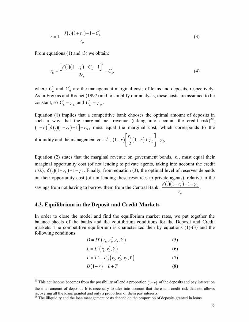
4.3. Equilibrium in the Deposit and Credit Markets In order to close the model and find the equilibrium market rates, we put together the balance sheets of the banks and the equilibrium conditions for the Deposit and Credit markets. The competitive equilibrium is characterized then by equations (1)-(3) and the following conditions:
( )*, , ,sD D TD D r r r Y= (5)
( )*, ,dL LL L r r Y= (6)
( )*, , ,s db D D TT T T r r r Y−= − (7)
( )1D r L T− = + (8)
20 This net income becomes from the possibility of lend a proportion ( )1 r− of the deposits and pay interest on the total amount of deposits. It is necessary to take into account that there is a credit risk that not allows recovering all the loans granted and only a proportion of them pay interests. 21 The illiquidity and the loan management costs depend on the proportion of deposits granted in loans.

9
where:
( )*, , ,sD D TD r r r Y is the total supply of deposits by the non-financial agents, which depends
positively on the domestic deposit interest rate and income, and negatively on the foreign deposit interest rate and the return on government securities. It is assumed that these two types of assets are imperfect substitutes of domestic deposits.
( )*, ,dL LL r r Y is the loan demand by the agents in the economy, that depends negatively on
the loan domestic interest rate and positively on the agents’ level of income. It also depends positively on foreign loans interest rates, which are assumed to be imperfect substitutes of domestic loans. T s is the exogenous supply of securities by the government and ( )*, , ,d
b D D TT r r r Y− is the demand of these securities by other agents in the economy. It depends positively on the income and the own return, and negatively on the interest rate paid by domestic and foreign deposits, considered as imperfect substitutes of these securities. Hence, in equilibrium:
( ) ( ) ( ) ( )* * *, , 1 , , , , , ,d s S d
L L D D T b D D TL r r Y r D r r r Y T T r r r Y−= − − + (9) The equilibrium deposit and loan interest rates are derived from equations (1), (2), (3) and (9), as implicit functions of the exogenous variables ( )* *, , , , , ,S
L L p c D L Dr r r r r T Y γ γ= and
( )* *, , , , , ,SD D p c D L Dr r r r r T Y γ γ= . These functions are potentially non-linear because they
depend on the functional forms of the deposit supply and loan demand22. 4.4. The Results The comparative statics analysis of equations (1)-(3) and (9) allows us to appreciate the effects of shocks to the exogenous variables on deposit and loan interest rates (see Appendix A for the details). Result 1: The effect of a shift in the monetary policy interest rate, rp , on the equilibrium loan interest rate is positive. The effect of the same shift on the deposit interest rate is ambiguous. An increase in the policy interest rate makes the liquidity shortage more costly for banks. This has two implications. On the one hand, banks have more incentives to keep a higher level of reserves, implying a decrease in banks’ loan supply or an increase in deposit demand. Hence, there is an upward pressure on loan and deposit interest rates. On the other hand, since the cost of illiquidity depends on the amount of deposits, the rise in policy rates
22 Also, these functions can be non-linear if the withdrawals have a non-uniform probability distribution.
10
makes deposits more expensive and reduces banks’ demand for them. This pushes deposit rates down. Result 2: A change in the foreign interest rates or the expectations of depreciation has a positive effect on equilibrium loan and deposit interest rates. If the foreign interest rates or the expectations of depreciation rise, agents in the domestic economy perceive a higher cost of borrowing abroad, increasing their demand for domestic loans. Thus, domestic loan interest rates increase. The higher demand for loans makes banks raise their deposit demand at the same time that agents reduce their supply of deposits because foreign deposits are more attractive. Hence, deposit interest rates also increase. Result 3: The effect of a change in the income level on the equilibrium loan and deposit interest rates is ambiguous. An increase in income raises deposit supply and loan demand, implying a decline in the deposit rate and an increase in the loan rate. In order to satisfy the higher demand for loans, banks increase their demand for deposits, pushing deposit interest rates up. Additionally, given that credit risk is reduced by the agents’ better conditions (a higher proportion of loans will be recovered), banks have incentives to increase their loan supply inducing a downward pressure on loan rates. As a result, the effect of the shift in income on market rates is ambiguous. Result 4: An increase in the government securities supply, T s , implies a rise in the equilibrium level of loan and deposit interest rates. An additional supply of government securities competes with loans in banks’ portfolios and with deposits in the agents’ portfolios. This implies a reduction in the supply of deposits by firms and households, and a drop in the loan supply by commercial banks, increasing interest rates. This effect is reinforced if banks increase their demand for deposits to fund their purchases of government securities. Notice that, in general, the response of market interest rates to the exogenous shocks may not be linear and could depend on macro variables affecting the elasticities of the loan demand and the supply for deposits. In other words, that response is complex and may depend on the state of the economy. Furthermore, it is possible that a shock to an exogenous variable has an impact on others. For example, an increase in the foreign interest rate may cause movements in the policy rate, the expectations of depreciation and output. Hence, the observed response of market rates to “a” shock may involve a reaction to movements in several variables. As a corollary, we conclude that there is a possibly complex relationship between policy and market interest rates. We also conclude that interest rate pass-through depends on the state of the economy and that its estimation must control for the presence of other shocks hitting the financial markets.
11
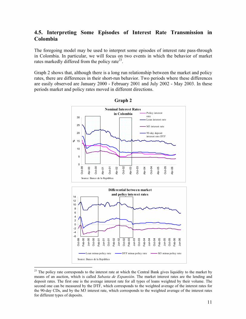
4.5. Interpreting Some Episodes of Interest Rate Transmission in Colombia The foregoing model may be used to interpret some episodes of interest rate pass-through in Colombia. In particular, we will focus on two events in which the behavior of market rates markedly differed from the policy rate23. Graph 2 shows that, although there is a long run relationship between the market and policy rates, there are differences in their short-run behavior. Two periods where these differences are easily observed are January 2000 - February 2001 and July 2002 - May 2003. In these periods market and policy rates moved in different directions.
Graph 2
23 The policy rate corresponds to the interest rate at which the Central Bank gives liquidity to the market by means of an auction, which is called Subasta de Expansión. The market interest rates are the lending and deposit rates. The first one is the average interest rate for all types of loans weighted by their volume. The second one can be measured by the DTF, which corresponds to the weighted average of the interest rates for the 90-day CDs, and by the M3 interest rate, which corresponds to the weighted average of the interest rates for different types of deposits.
Nominal Interest Rates in Colombia
0
5
10
15
20
25
30
Oct
-99
Abr-
00
Oct
-00
Abr-
01
Oct
-01
Abr-
02
Oct
-02
Abr-
03
Oct
-03
Abr-
04
Oct
-04
Abr-
05
Oct
-05
Abr-
06
%
Policy interestrateLoan interest rate
M3 interest rate
90-day depositinterest rate DTF
Source: Banco de la República
Differential between market and policy interest rates
-6-4-202468
101214
Oct
-99
Feb-
00
Jun-
00
Oct
-00
Feb-
01
Jun-
01
Oct
-01
Feb-
02
Jun-
02
Oct
-02
Feb-
03
Jun-
03
Oct
-03
Feb-
04
Jun-
04
Oct
-04
Feb-
05
Jun-
05
Oct
-05
Feb-
06
Jun-
06
Loan minus policy rate DTF minus policy rate M3 minus policy rate
Source: Banco de la República

12
January 2000-February 2001: During this period the monetary policy interest rate was stable, while market interest rates were increasing24. At the same time, the real quantities of loans and deposits in the financial system were going down. These facts suggest shifts of loan and deposit supplies larger than the shifts in their respective demands. This is the period immediately after a deep recession and a financial crisis characterized by a sharp deterioration of loan quality. At the same time, there was a large increase in the supply of Government domestic bonds. As a consequence, the banks´ risk perceptions of the economy soared, their holdings of Government securities rose and loan supply dried. This implied a cut in the banks´ demand for deposits that, however, was more than compensated by the reduction in the supply that followed the increase in country risk, the rise in foreign interest rates, the presence of a high depreciation of the currency and the growing supply of Government domestic debt (Graph 3).
Graph 3.
24 In the beginning of the period market interest rates continued their decreasing trend for one month and then changed their behavior. The lending interest rate was stable during four months and then increased by 280 basis points. The deposit interest rates increased since February 2000. Specifically, the CD rates (DTF) went up by 313 basis points.
Loan Quality
-
2
4
6
8
10
12
14
16
18
20
Mar
-98
Sep-
98
Mar
-99
Sep-
99
Mar
-00
Sep-
00
Mar
-01
Sep-
01
Mar
-02
Sep-
02
Mar
-03
Sep-
03
Mar
-04
Sep-
04
Mar
-05
Sep-
05
Mar
-06
%
Source: Banco de la República
Government Securities/Total Financial Sector Assets
0
3
6
9
12
15
18
21
24
Ene-
99
Jul-9
9
Ene-
00
Jul-0
0
Ene-
01
Jul-0
1
Ene-
02
Jul-0
2
Ene-
03
Jul-0
3
Ene-
04
Jul-0
4
Ene-
05
Jul-0
5
Ene-
06
Source: Banco de la República
%
Nominal Foreign Interest Rate (US$)
0
1
2
3
4
5
6
7
8
9
10
11O
ct-9
9
Feb-
00
Jun-
00
Oct
-00
Feb-
01
Jun-
01
Oct
-01
Feb-
02
Jun-
02
Oct
-02
Feb-
03
Jun-
03
Oct
-03
Feb-
04
Jun-
04
Oct
-04
Feb-
05
Jun-
05
Oct
-05
Feb-
06
Jun-
06
%
PRIMELIBOR
Source: Datastream
EMBI Colombia and Nominal Depreciation
-25
-15
-5
5
15
25
35
Oct
-99
Feb-
00
Jun-
00
Oct
-00
Feb-
01
Jun-
01
Oct
-01
Feb-
02
Jun-
02
Oct
-02
Feb-
03
Jun-
03
Oct
-03
Feb-
04
Jun-
04
Oct
-04
Feb-
05
Jun-
05
Oct
-05
Feb-
06
Jun-
06
0
100
200
300
400
500
600
700
800
900
1000
Anual Depreciation
Embi Colombia
Source: Bloomberg and Banco de la República

13
July 2002 - May 2003: During this period, a sharp increase in country risk occurred that pushed up the depreciation of the currency. At the same time, growth recovered (Graph 4) and the quality of the loan portfolio continued to improve. Market rates slightly declined, while policy rates were kept constant until December 2002, and then were raised by 200 bps to curb inflationary pressures stemming from the depreciation of the currency. The real quantities of deposits and loans showed small increases. The increase in output growth and a better perception of the risk of the financial system pushed up the supply of deposits. This movement and the improvement in loan quality may have produced a positive shift in the loan supply. These factors would have implied a reduction in market interest rates, given a constant policy rate25. However, the skyrocketing country risk and the ensuing depreciation exerted an upward pressure on interest rates that countered the previous effect. The jump in country risk also produced a loss of market value of Government securities that may have increased the supply of deposits, as agents rebalanced their portfolio away from Government debt and in favor of financial system liabilities. In the second part of the period, this shift was reinforced when country risk plummeted. Market interest rates must have declined, but then policy rates were raised, offsetting this trend.
Graph 4.
GDP Anual Growth
-8,0
-6,0
-4,0
-2,0
0,0
2,0
4,0
6,0
8,0
Mar
-98
Jul-9
8
Nov
-98
Mar
-99
Jul-9
9
Nov
-99
Mar
-00
Jul-0
0
Nov
-00
Mar
-01
Jul-0
1
Nov
-01
Mar
-02
Jul-0
2
Nov
-02
Mar
-03
Jul-0
3
%
Source: DANE
25 A higher economic growth may have also pushed loan demand. However, after the financial crisis there was a process of reduction in the leverage of the private sector.

14
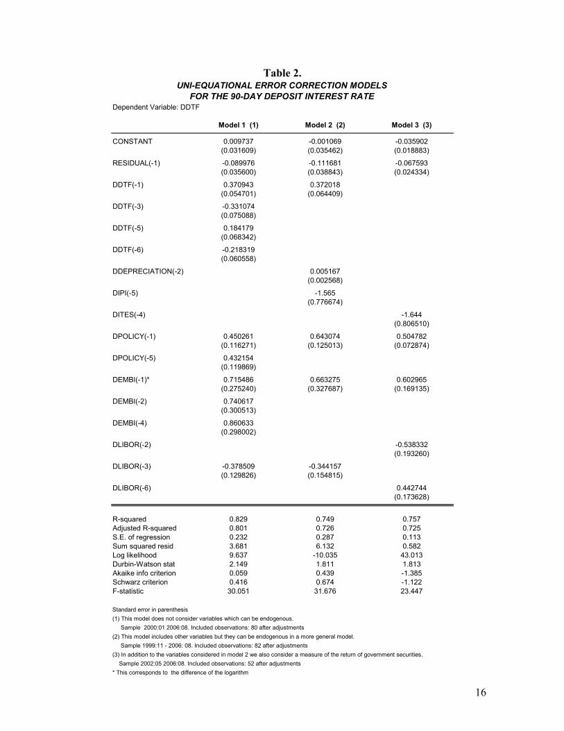
5. Econometric Evidence The theoretical model developed in the previous section implies that market interest rates are affected by factors other than the policy rate. Therefore, the estimation of interest rate pass-through must control for movements in other macroeconomic variables, which may impact the loan and deposit markets equilibrium. To test this hypothesis, we follow two approaches. First, we assume the existence of a long run relationship between market and policy interest rates. Then we estimate uni-equational error correction models for the market rates, in which other macro variables suggested by the theoretical model are included as explanatory variables of the short run dynamics (See Appendix D for the description of the variables). In the second approach we acknowledge that some of the macro explanatory variables may be endogenous in a general equilibrium context. Hence, we estimate a VARX, perform Granger causality tests for the market interest rate equation to verify the significance of the macro variables in determining its dynamics, and examine the impulse response functions to check the direction of the market interest rate reaction to different shocks. 5.1. Uni-equational Error Correction Models For both measures of the deposit interest rate, DTF and M3, we estimate uni-equational error correction models for the period June 1999-August 2006, with the policy interest rate, the industrial production index (as a measure of output), the EMBI, the foreign interest rate (LIBOR) and the nominal depreciation as explanatory variables. We also use a measure of the price change of Government securities as another exogenous variable. However, because this variable is only available from 2001 on, we decided to estimate another model with this shorter sample. Tables 1 and 2, show the estimations of different models for each measure of the deposit interest rate. The first model takes as explanatory variables the EMBI, the LIBOR and the Policy interest rate, which can be assumed to be exogenous in a more general model. The second model also includes the nominal depreciation and the industrial production index as exogenous variables, eventhough they can be endogenous in a more general setting. Finally, the third model was estimated for DTF introducing the price change of Government securities. In most cases, variables different from the policy interest rate and the residual of the long run equation26 are significant in the error correction equations. Hence, the short run dynamics of deposit interest rates are influenced by other macro variables, as suggested by the theoretical model developed above. Also, in most cases the signs of the exogenous variables are those predicted by the theory, with the notable exception of the foreign interest rate.
26 This residual is obtained from the estimation of the long run relationship between the policy and the deposit interest rate.

15
Table 1.
Dependent Variable: DM3
Model 1 (1) Model 2 (2)
CONSTANT 0.003631 -0.007897(0.032964) (0.029407)
RESIDUAL(-1) -0.092387 -0.113488(0.045228) (0.041106)
DDEPRECIATION(-1) 0.008027(0.002196)
DDEPRECIATION(-4) 0.006092(0.002350)
DPOLICY(-1) 0.272142 0.243948(0.118982) (0.109475)
DPOLICY(-2) 0.620527 0.576526(0.108078) (0.099845)
DEMBI(-1)* 0.626833(0.283245)
DEMBI(-4) 0.742623 0.686215(0.289368) (0.295535)
DLIBOR(-4) -0.382553(0.120717)
R-squared 0.675 0.746Adjusted R-squared 0.654 0.722S.E. of regression 0.257 0.230Sum squared resid 5.042 3.945Log likelihood -2013 8.049Durbin-Watson stat 1.461 1.517Akaike info criterion 0.195 -0.001203Schwarz criterion 0.371 0.233599F-statistic 31.676 31.099
Standard error in parenthesis(1) This model does not consider variables which can be endogenous. Sample 1999:11 2006:08. Included observations: 82 after adjustments(2) This model includes other variables but they can be endogenous in a more general model. Sample 1999:11 - 2006: 08. Included observations: 82 after adjustments* This corresponds to the difference of the logarithm
UNI-EQUATIONAL ERROR CORRECTION MODELS FOR THE M3 INTEREST RATE
16
Table 2.
Dependent Variable: DDTF
Model 1 (1) Model 2 (2) Model 3 (3)
CONSTANT 0.009737 -0.001069 -0.035902(0.031609) (0.035462) (0.018883)
RESIDUAL(-1) -0.089976 -0.111681 -0.067593(0.035600) (0.038843) (0.024334)
DDTF(-1) 0.370943 0.372018(0.054701) (0.064409)
DDTF(-3) -0.331074(0.075088)
DDTF(-5) 0.184179(0.068342)
DDTF(-6) -0.218319(0.060558)
DDEPRECIATION(-2) 0.005167(0.002568)
DIPI(-5) -1.565(0.776674)
DITES(-4) -1.644(0.806510)
DPOLICY(-1) 0.450261 0.643074 0.504782(0.116271) (0.125013) (0.072874)
DPOLICY(-5) 0.432154(0.119869)
DEMBI(-1)* 0.715486 0.663275 0.602965(0.275240) (0.327687) (0.169135)
DEMBI(-2) 0.740617(0.300513)
DEMBI(-4) 0.860633(0.298002)
DLIBOR(-2) -0.538332(0.193260)
DLIBOR(-3) -0.378509 -0.344157(0.129826) (0.154815)
DLIBOR(-6) 0.442744(0.173628)
R-squared 0.829 0.749 0.757Adjusted R-squared 0.801 0.726 0.725S.E. of regression 0.232 0.287 0.113Sum squared resid 3.681 6.132 0.582Log likelihood 9.637 -10.035 43.013Durbin-Watson stat 2.149 1.811 1.813Akaike info criterion 0.059 0.439 -1.385Schwarz criterion 0.416 0.674 -1.122F-statistic 30.051 31.676 23.447
Standard error in parenthesis(1) This model does not consider variables which can be endogenous. Sample 2000:01 2006:08. Included observations: 80 after adjustments(2) This model includes other variables but they can be endogenous in a more general model. Sample 1999:11 - 2006: 08. Included observations: 82 after adjustments(3) In addition to the variables considered in model 2 we also consider a measure of the return of government securities. Sample 2002:05 2006:08. Included observations: 52 after adjustments* This corresponds to the difference of the logarithm
UNI-EQUATIONAL ERROR CORRECTION MODELS FOR THE 90-DAY DEPOSIT INTEREST RATE

17
However, to assess the impact of exogenous shocks on market rates, one must take into account not only their direct effect on deposit rates, but also the indirect effects that occur through other macro variables that are endogenous in a general equilibrium context, such as the exchange rate, output and expectations. There may be also feed-back from market rates themselves to those macro endogenous variables. To capture the richer dynamics implied by the argument above, we estimate a VARX for a set of variables in first differences. We assume that the EMBI, the foreign interest rates and the policy rates are exogenous variables, while deposit rates, inflation, nominal depreciation and our measure of output are treated as endogenous (and the return on government securities when included). In order to verify our hypothesis, we check the significance of variables other than the policy rate in the deposit rate equation by means of Granger causality tests. Then, from the impulse-response functions we examine the impact of some shocks on deposit rates. In this context, the response to a shift in the policy rate may be regarded as an appropriate measure of interest rate pass-through, since most direct and indirect effects are taken into account. 5.2. VARX models Tables 3 and 4 show the Granger Causality tests for two specifications of VARX that include DTF or the M3 interest rates, respectively. In each case a system was estimated with and without the price change of Government bonds.27 For the DTF equation, the policy rate, the nominal depreciation and the EMBI Granger cause this deposit rate when the larger sample is used28. With the shorter sample, the policy rate, the nominal depreciation, the industrial production index, the EMBI, and the price change of Government securities Granger cause the DTF rate (Table 3). The equation for the M3 interest rate shows that the policy rate, inflation, nominal depreciation and the EMBI Granger-cause this deposit rate in the larger sample29. For the shorter sample, the policy rate, the industrial production index, the EMBI, the price change of Government securities and the foreign interest rate Granger cause the M3 rate (Table 4). The impulse-response functions of the VARX for the DTF and M3 interest rates are presented in Appendix B and show a positive short-run reaction of market rates to policy rate shocks. For other shocks, the market interest rates short-run response is sometimes in agreement with the theoretical model. In particular, there is a positive response of the DTF rate to shocks to the EMBI.
27 There may exist a bias in the estimation because we are not taking into account the long run relationship between market and policy interest rates and other long run relations between the variables included in the VARX. A method that allows to estimate the correct long and short run relationships is a VEC, but the sample is too short to use this technique. 28 At 10% of significance inflation also Granger causes the DTF. 29 At 10% of significance the foreign interest rate (Libor) also Granger causes the M3 interest rate.

18
Table 3.
Null Hypothesis Test-value Probability
DDEPRECIATION not Granger cause DDTF 26.56 0.0002
DIPI not Granger cause DDTF 3.62 0.7284
DINFLATION not Granger cause DDTF 11.02 0.0878
DEMBI not Granger cause DDTF 13.58 0.0592
DPOLICY not Granger cause DDTF 88.14 0.0001
DLIBOR not Granger cause DDTF 3.70 0.8136
* VARX(6,6) 6 lags for endogenous and exogenous variables
Null Hypothesis Test-value Probability
DDEPRECIATION not Granger cause DDTF 9.93 0.0191
DIPI not Granger cause DDTF 7.87 0.0489
DINFLATION not Granger cause DDTF 5.67 0.1288
DITES not Granger cause DDTFN 22.19 0.0001
DEMBI not Granger cause DDTF 14.48 0.0059
DPOLICY not Granger cause DDTF 12.28 0.0154
DLIBOR not Granger cause DDTF 7.38 0.1171
* VARX(3,3) 3 lags for endogenous and exogenous variables
Model 2
Granger Causality Tests on DTF
Granger Causality Tests on DTF
Model 1
Table 4.
Null Hypothesis Test-value Probability
DDEPRECIATION not Granger cause DM3 25.78 0.0002
DIPI not Granger cause DM3 10.43 0.1077
DINFLATION not Granger cause DM3 27.80 0.0001
DEMBI not Granger cause DM3 18.80 0.0088
DPOLICY not Granger cause DM3 87.14 0.0001
DLIBOR not Granger cause DM3 12.78 0.0778
* VARX(6,6) 6 lags for endogenous and exogenous variables
Null Hypothesis Test-value Probability
DDEPRECIATION not Granger cause DM3 1.84 0.7656
DIPI not Granger cause DM3 10.88 0.0279
DINFLATION not Granger cause DM3 5.84 0.2113
DITES not Granger cause DDTFN 15.66 0.0035
DEMBI not Granger cause DM3 23.86 0.0001
DPOLICY not Granger cause DM3 52.19 0.0001
DLIBOR not Granger cause DM3 12.62 0.0133
* VARX(4,3) 4 lags for endogenous and 3 lags for exogenous variables
Model 1
Model 2
Granger Causality Tests on M3
Granger Causality Tests on M3

19
6. A Small-Open Economy Macro Model In section 4 we showed that the equilibrium market interest rates depend not only on policy rates, but also on other macro variables affecting credit demand and deposit supply, such as income, external interest rates, risk premia and the expectations of inflation and real depreciation among others. These are exogenous variables in a partial equilibrium setting, but some become endogenous once one considers the functioning of the economy as a whole. Hence, interest rate pass-through may be a complex process, with changes in policy having both direct and indirect effects on market rates, the latter taking place through shifts in income, depreciation, inflation and expectations. By the same token, shocks hitting the economy may have direct effects on market interest rates, given a constant policy rate. For example, an increase in external interest rates or the country risk premium will affect not only the exchange rate, as expected, but also market interest rates, since deposits and central bank credit are imperfect substitutes for banks due to the liquidity risk. Were they perfect or very close substitutes, the domestic interest rates would be set by the Central Bank and all the adjustment will be born by the exchange rate. In addition, the model developed in section 4 suggested that the relationship between policy and market interest rates might not be “one for one”, or even linear. That relationship depends on the functional forms of the demand for credit, the supply of deposits and the probability distributions involved in the various risks facing the banking firm. This further complicates the interest rate pass-through. A policy implication follows immediately from the previous arguments: The Central Bank´s policy rule should take into account the direct effects of other (exogenous and endogenous) macro variables on market rates. It should also consider the possibly complex relationship between policy and market rates. If these factors are empirically relevant, a failure by the Central Bank to include them in its reaction function may increase the risk of missing its targets and/or may introduce excessive volatility to interest rates and output. These ideas can be illustrated with a simpler version of the model presented above. In particular, assume that there is neither credit risk nor public debt. There is only a liquidity risk for banks. Deposit interest rates are determined by the equilibrium conditions in the deposit and credit markets and the balance sheet identity of the banking sector:
( )^ ^
* *( , , ) 1 ( , ) ( , , )e e e e e e e eD D p DD i i e Y r i i C i m i e Yπ π π π π π− + − − − − = − + + − (10)
Where D(.) and C(.) are the deposit supply and credit demand functions, respectively. r(.) is the fraction of deposits that banks optimally choose to hold as reserves. Y is the level of output. iD and ip are the nominal deposit and policy rate, respectively. m is a constant intermediation spread that accounts for operational costs. i* is the external nominal interest
rate and ^ee and πe are the expectations of depreciation and inflation, respectively. As in
section 4, the following assumptions are made about the functional forms:

20
*
*
0, 0, 0
0, 0, 0D
D
i Yi
i Yi
D D D
C C C
> < >
< > >
And the following features of the function r(.) are obtained: 0, 0
D pi ir r< >
Starting from a long run equilibrium situation in which π = πe = πTARGET, suppose that there is a transitory shock to the external interest rate, i*, and that the Central Bank is a “strict inflation targeter” that will move its policy rate, ip, so that the inflation target is met at every period. Furthermore, assume that the public fully trust the inflation target. In these
circumstances, 0** ==did
did eππ . Assuming that the Central Bank knows all the parameters
and the structure of the economy, from equation (10) the required adjustment of the policy rate is given by:
( ) ( ) ( ) ( )* *
^1
* * * *(1 ) 1 (1 ) (1 )p D D D
ep D
i i i i Y Yi i
di did e dYD r D r C D r D r C D r Cdi di di di
− = − − + + − − − + − −
(11)
Where *didiD is the adjustment in the deposit rate that is required to keep inflation on target.
*didY is the change in output that results from the shock to the foreign interest rate, i*, the
responses of iD and ip and all the subsequent macroeconomic effects. Similarly, *
^
died e
is the
movement of the expectations of depreciation that follows the shock to i*, the responses of iD and ip and all the ensuing macroeconomic effects. Three results are obtained from equation (11):
(i) The “direct” response of the policy rate to the required adjustment in the market rate is not necessarily equal to one. The expression ( ) ( )(1 )
D D D pi i i iD r D r C D r− − − is generally positive, but may not even be
constant. It may change with the levels of Y, iD, i* and other variables that might affect the elasticities or “slopes” of credit demand, deposit supply and reserves demand.
(ii) Beyond the “direct” response to the required adjustment in the market rates,
policy rates may have to respond independently to the shock itself. The term ( ) ( )* *(1 )
pii iD r C D r− − is generally negative, suggesting a negative reaction of
policy rates to the shift in external interest rates. Intuitively, if market rates react directly to the shock in foreign interest rates, Central Bank rates do not
21
change in the expectations of depreciation that results from the shock and the ensuing adjustment.
(iii) Also, policy interest rates may respond to the change in output that follows the
shock. In this case, however, the effect on policy rates is ambiguous since, as shown in section 4, changes in output hit both loan demand and deposit supply, inducing movements of market rates in opposite directions.
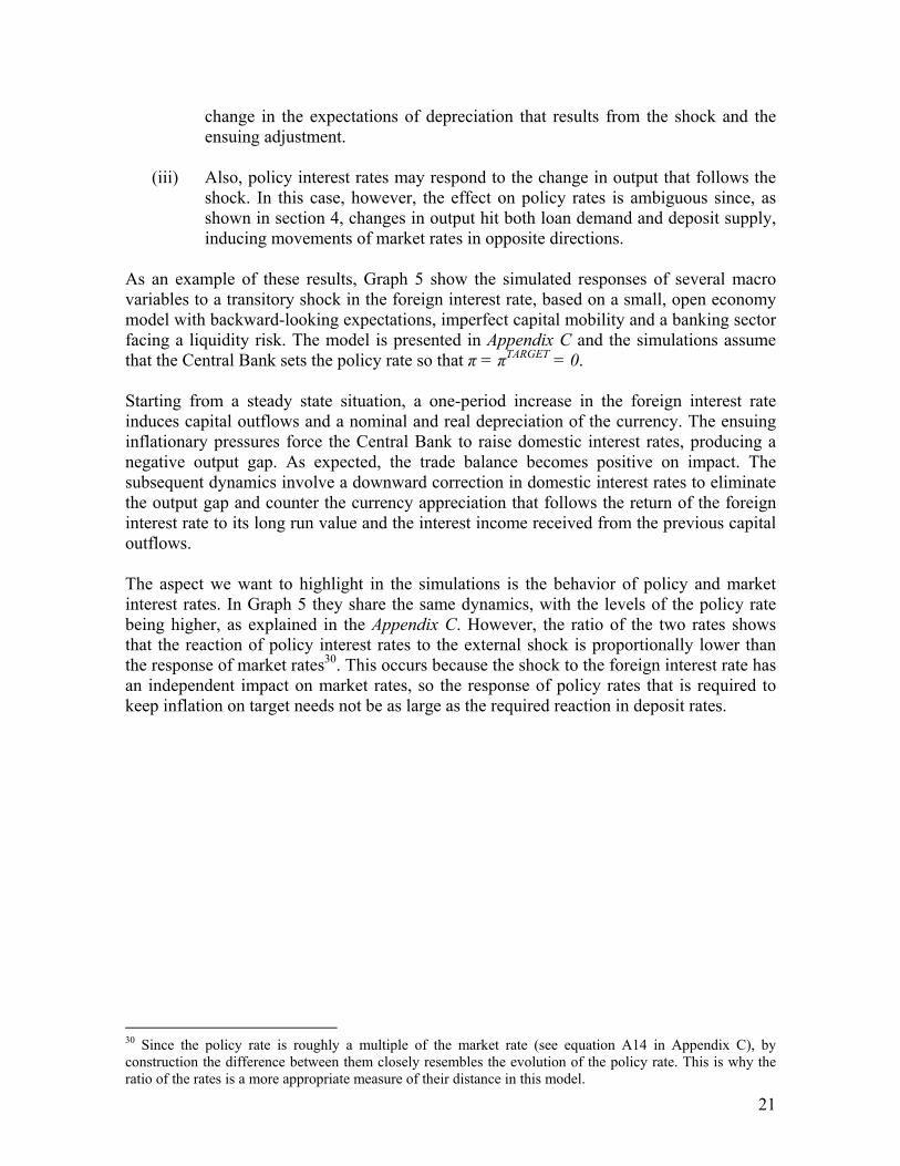
As an example of these results, Graph 5 show the simulated responses of several macro variables to a transitory shock in the foreign interest rate, based on a small, open economy model with backward-looking expectations, imperfect capital mobility and a banking sector facing a liquidity risk. The model is presented in Appendix C and the simulations assume that the Central Bank sets the policy rate so that π = πTARGET = 0. Starting from a steady state situation, a one-period increase in the foreign interest rate induces capital outflows and a nominal and real depreciation of the currency. The ensuing inflationary pressures force the Central Bank to raise domestic interest rates, producing a negative output gap. As expected, the trade balance becomes positive on impact. The subsequent dynamics involve a downward correction in domestic interest rates to eliminate the output gap and counter the currency appreciation that follows the return of the foreign interest rate to its long run value and the interest income received from the previous capital outflows. The aspect we want to highlight in the simulations is the behavior of policy and market interest rates. In Graph 5 they share the same dynamics, with the levels of the policy rate being higher, as explained in the Appendix C. However, the ratio of the two rates shows that the reaction of policy interest rates to the external shock is proportionally lower than the response of market rates30. This occurs because the shock to the foreign interest rate has an independent impact on market rates, so the response of policy rates that is required to keep inflation on target needs not be as large as the required reaction in deposit rates.
30 Since the policy rate is roughly a multiple of the market rate (see equation A14 in Appendix C), by construction the difference between them closely resembles the evolution of the policy rate. This is why the ratio of the rates is a more appropriate measure of their distance in this model.

22
Graph 5.
5 10 15 20 25 30 35t
0.022
0.024
0.026
0.028
0.03
0.032
0.034
ix Foreign interest rate
5 10 15 20 25 30 35t
0.022
0.024
0.026
0.028
0.03
0.032
0.034
id Domestic interest rate
5 10 15 20 25 30 35t
0.045
0.05
0.055
0.06
0.065
0.07
0.075ip Policy interest rate
5 10 15 20 25 30 35t
0.474
0.475
0.476
0.477
0.478
0.479
id�ip Domestic �Policy int.rates ratio
5 10 15 20 25 30 35t
-0.001
-0.0008
-0.0006
-0.0004
-0.0002
0.0002
0.0004
y Output gap
5 10 15 20 25 30 35t
-0.003
-0.002
-0.001
0.001
0.002
0.003
0.004e Nominal Depreciation
5 10 15 20 25 30 35t
-0.002
0.002
0.004
q Real Exchange Rate
5 10 15 20 25 30 35t
-0.0004
-0.0002
0.0002
0.0004
nx Trade Balance

23
7. Conclusions In contrast to the standard approach to monetary policy, which considers the banking sector as a passive aggregate, this paper focused on the implications of modeling commercial banks as independent entities that optimally react to their environment. Based on a theoretical microeconomic model of the banking firm and the credit and deposits markets, we illustrated the idea that the response of market interest rates to changes in the policy interest rate may be a complex process that depends on the state of the economy. We argued that the estimation of interest rate pass-through must control for other shocks hitting the financial system. The model is used to interpret some episodes of interest rate pass-through in Colombia and the results from uni-equational error correction and VARX models seem to support our hypotheses. Finally, a small macro model illustrated the importance for the Central Bank to understand the role of bank behavior in the interest rate pass-through. In particular, consideration of the direct impact of exogenous shocks on the financial system may affect the appropriate policy response. Depending on its empirical relevance, this hypothesis implies that the Central Bank may miss its targets or introduce excessive volatility to interest rates and output, if financial market behavior is ignored.

24
8. Bibliography Ahumada, L., and J.R. Fuentes, “Banking Industry and Monetary Policy: An Overwiew”, In: Banking Market Structure and Monetary Policy, Central Bank of Chile, 2004. Amaya, C.A., “Interest Rate Setting and the Colombian Monetary Transmission Mechanism”, Banco de la República Colombia, Borradores de Economía, No 352, 2005. Bernanke, B., and A. Blinder, “Credit, Money and Aggregate Demand”, American Economic Review, Vol. 78, No. 2, 1988. Bernanke , B., and M. Gertler, “Inside the Black Box: The Credit Channel of Monetary Policy Transmission”, Journal of Economic Perspectives, Vol 9, No 4, 1995. Berstein, S., and R. Fuentes, “Is there Lending Rate Stickiness in the Chilean Banking Industry?”, Central Bank of Chile Working Papers, No 218, 2003. Cottarelli, C., and A. Kourelis, “Financial Structure, Bank Lending Rates, and the Transmission Mechanism of Monetary Policy”, IMF Staff Papers, Vol 41, No 4, 1994. Crespo-Cuaresma, J., et al., “Interest Rate Pass-Through in New EU Member Status: The Case of the Czech Republic, Hungary and Poland”, William Davidson Institute, University of Michigan Business School, Working Paper, No 671, 2004. De Bondt, G., “Retail Bank Interest Rate Pass-Through: New Evidence at the Euro Area Level”, European Central Bank Working Paper Series, No 136, 2002. De Bondt, G., “Interest Rate Pass-Through: Empirical results for the Euro Area”, German Economic Review, Vol 6, No 1, 2005. Ehrmann, M., and A. Worms, “Interbank lending and Monetary Policy Transmission evidence for Germany”, Economic Research Centre of the Deutsche Bundesbank, Discussion Paper No. 11, 2001. Engle, R., and B.S. Yoo, “Forecasting and Testing in Coi-integrated Systems”, Journal of Econometrics, 35, 1987. Freixas X., and J.C. Rochet, “Microeconomics of Banking”, MIT Press, Cambridge, 1997. Hannan, T., and A. Berger, “The Rigidity of Prices: Evidence from the Banking Industry”, American Economic Review, Vol 81, No 4, 1991. Huertas et al., “Algunas Consideraciones sobre el Canal de Crédito y la Transmisión de Tasas de Interés en Colombia, Banco de la República Colombia, Borradores de Economía, No 351, 2005.

25
Julio, J.M., “Relación entre la Tasa de Intervención del Banco de la República y las Tasas del Mercado: Una Exploración Empírica”, Banco de la República Colombia, Borradores de Economía, No 188, 2001. Kot, A., “Is Interest Rate Pass-Through related to Banking Sector Competitiveness?”, National Bank of Poland, 2004. Kwapil, C., and J. Scharler, “Interest Rate Pass-Through, Monetary Policy Rules and Macroeconomic Stability”, Austrian Central Bank Working Papers, No 118, 2005. Loayza, N., and K. Schmidt-Hebbel, “Monetary Policy Functions and Transmission Mechanisms: An Overview”, In: Monetary Policy: Rules and Transmission Mechanisms, Central Bank of Chile, 2002. Mojon, B., “Financial Structure and the Interest Rate Channel of ECB Monetary Policy”, European Central Bank Working Paper Series, No 40, 2000. Sorensen, C.K., and T. Werner, “Bank Interest Rate Pass-Through in the Euro Area: A Cross Country Comparison”, European Central Bank Working Paper Series, No 580, 2006. Stiglitz, J. and A. Weiss, “Credit Rationing in markets with imperfect information”, American Economic Review, Vol 71, No 3, 1981. Villar, L., et al., “Crédito, Represión Financiera y Flujos de Capitales en Colombia: 1974-2003”, Banco de la República Colombia, Borradores de Economía, No 322, 2005. Weth, M., “The Pass-Through from market interest rates to bank lending rates in Germany”, Economic Research Centre of the Deutsche Bundesbank, Discussion Paper No. 11, 2002. Winker, P., “Sluggish Adjustment of Interest Rates and Credit Rationing: An Application of Unit Root Testing and Error Correction Modelling”, Applied Economics, 31, 1999. Zamudio, N., and J. Martinez, “Estructura Financiera de las Empresas y los Hogares 2004-2005”, Mimeo, Banco de la República Colombia, 2006.

26
Appendix A
The Micro-Banking Model
A.1. Effect of a marginal shift in the monetary policy interest rate: Differentiating equation (8) with respect to rp yields the following result:
( ) ( )
( ) ( ) ( )
1 .
1 1 .
dssbD
p D D pLd dd s s
sp b bD T
L L D D L T T L
Tr D rr Dr r r rdr
dr T Tr rL D D rr r Dr r r r r r r r
−
− −
∂∂ ∂ ∂− + − ∂ ∂ ∂ ∂ =
∂ ∂∂ ∂∂ ∂ ∂ ∂− − + − − + + ∂ ∂ ∂ ∂ ∂ ∂ ∂ ∂
(A1)
where:
(i) ( )( ) 2
2
. 1 10
2L LD
p p
rrr r
δ γ+ − − ∂ = − <∂
is the direct impact of the policy rate on the
deposit rate. This effect is negative because a higher policy rate implies a higher illiquidity cost and, as the withdrawals depend on the amount of deposits, banks will demand deposits only at lower deposit rates.
(ii) ( ) ( ). 1TL
L L
r rr r
δδ∂ ∂= + +
∂ ∂ is the impact of the loan interest rate on the government
securities return, which is ambiguous because a positive shift in loan interest rates
implies an increase in the credit risk, ∂δ∂rL
< 0 . However, if the economic conditions
are good, the proportion of recovered loans ( ).δ can be sufficiently high to
compensate the increasing credit risk, so that, ∂rT
∂rL
will be positive. Intuitively,
( ) ( ). 1 LL
rrδδ ∂
+ +∂
is the bank’s marginal revenue derived from an increase in rL . If
it is positive, banks will increase loans, demand less government bonds and the price of the latter will fall ( rT will go up).
(iii) ( ) ( ). 1 L
L
L p
rrr
r r
δδ ∂
+ + ∂∂ = −∂
is the impact of the loan interest rate on the banks’
fraction of reserves It is also ambiguous and depends on credit risk. As before, if the increase in credit risk is smaller than the recovered proportion of loans, this effect is
27
negative. Intuitively, if the bank’s revenues increase with the rise in rL , banks will lend more and reduce reserves.
(iv) ( )( )( ) ( ) ( ). 1 1 . 1L L L
LD
L p
r rrr
r r
δδ γ δ ∂
+ − − + + ∂∂ =∂
is the impact of loan interest rate
on deposit rates. From equation (2), we know that ( )( )( ). 1 1L Lrδ γ+ − − is positive if there are positive returns on government securities. Additionally, as before, if
( ) ( ). 1 LL
rrδδ
∂+ + ∂
>0, then ∂rD
∂rL
> 0 . Intuitively, if the bank’s revenues increase
with the rise in rL , they will demand more deposits inducing an upward pressure on rD .
(v) ( )( )( )
2
. 1 1L L
p p
rrr r
δ γ+ − −∂=
∂ is the direct impact of the policy rate on the proportion
of reserves, which is positive if rT > 0 . If the policy rate increases, the illiquidity cost goes up, and banks prefer to keep a higher proportion of deposits as reserves.
Finally,
drL
drp
is positive if ( ) ( ). 1 LL
rrδδ
∂+ + ∂
>0 and the own elasticity on the demand
for deposits (demand for government securities) is greater than the cross-elasticity with respect to the return on government securities (the deposit interest rate), namely,
∂Ds
∂rD
>∂T−b
d
∂rD
and
∂Ds
∂rT
<∂T−b
d
∂rT
. Thus we suppose that agents react more to the own
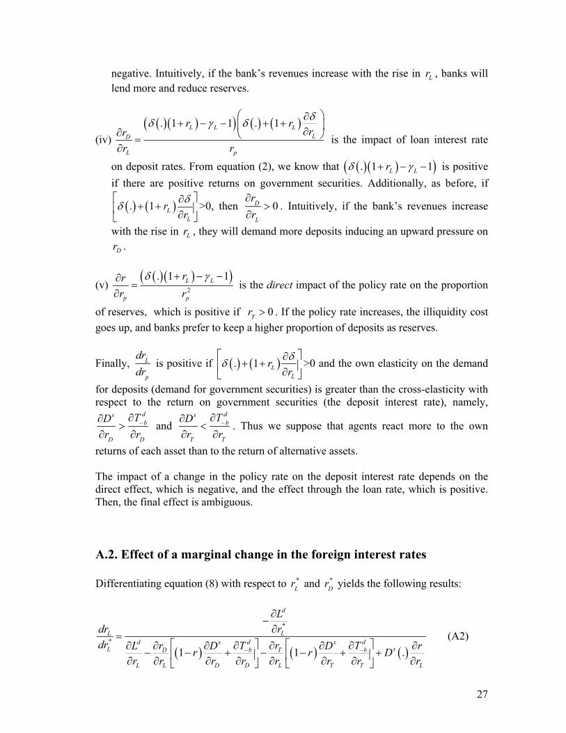
returns of each asset than to the return of alternative assets. The impact of a change in the policy rate on the deposit interest rate depends on the direct effect, which is negative, and the effect through the loan rate, which is positive. Then, the final effect is ambiguous. A.2. Effect of a marginal change in the foreign interest rates
Differentiating equation (8) with respect to rL
* and rD* yields the following results:
( ) ( ) ( )
*
*
1 1 .
d
L Ld dd s s
sL b bD T
L L D D L T T L
Ldr rdr T Tr rL D D rr r D
r r r r r r r r− −
∂−∂
= ∂ ∂∂ ∂∂ ∂ ∂ ∂
− − + − − + + ∂ ∂ ∂ ∂ ∂ ∂ ∂ ∂
(A2)
28
( )
( ) ( ) ( )
* *
*
1
1 1 .
dsb
L D Dd dd s s
sD b bD T
L L D D L T T L
TDrdr r rdr T Tr rL D D rr r D
r r r r r r r r
−
− −
∂∂− +
∂ ∂=
∂ ∂∂ ∂∂ ∂ ∂ ∂− − + − − + + ∂ ∂ ∂ ∂ ∂ ∂ ∂ ∂
(A3)
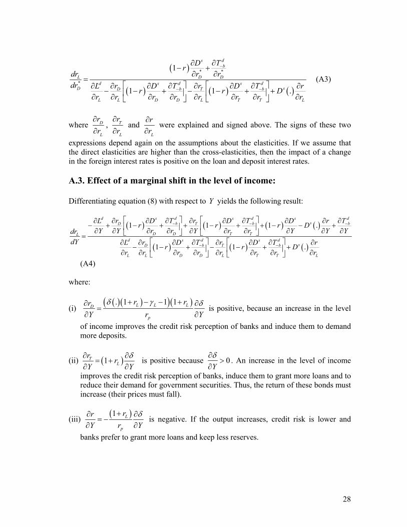
where
∂rD
∂rL
,
∂rT
∂rL
and
∂r∂rL
were explained and signed above. The signs of these two
expressions depend again on the assumptions about the elasticities. If we assume that the direct elasticities are higher than the cross-elasticities, then the impact of a change in the foreign interest rates is positive on the loan and deposit interest rates.
A.3. Effect of a marginal shift in the level of income: Differentiating equation (8) with respect to Y yields the following result:
( ) ( ) ( ) ( )
( ) ( ) ( )
1 1 1 .
1 1 .
d d dd s s ssb b bD T
D D T TLd dd s s
sb bD T
L L D D L T T L
T T Tr rL D D D rr r r DY Y r r Y r r Y Y Ydr
dY T Tr rL D D rr r Dr r r r r r r r
− − −
− −
∂ ∂ ∂∂ ∂∂ ∂ ∂ ∂ ∂− + − + + − + + − − + ∂ ∂ ∂ ∂ ∂ ∂ ∂ ∂ ∂ ∂ =
∂ ∂∂ ∂∂ ∂ ∂ ∂− − + − − + + ∂ ∂ ∂ ∂ ∂ ∂ ∂ ∂
(A4) where:
(i) ( )( )( )( ). 1 1 1L L LD
p
r rrY r Y
δ γ δ+ − − +∂ ∂=
∂ ∂ is positive, because an increase in the level
of income improves the credit risk perception of banks and induce them to demand more deposits.
(ii) ( )1TL
r rY Y
δ∂ ∂= +
∂ ∂ is positive because
∂δ∂Y
> 0 . An increase in the level of income
improves the credit risk perception of banks, induce them to grant more loans and to reduce their demand for government securities. Thus, the return of these bonds must increase (their prices must fall).
(iii) ( )1 L
p
rrY r Y
δ+∂ ∂= −
∂ ∂ is negative. If the output increases, credit risk is lower and
banks prefer to grant more loans and keep less reserves.

29
Although the previous assumptions about the elasticities are made,
drL
dY is ambiguous,
because agents are going to demand more credit,∂Ld
∂Y> 0 , at the same time that banks
grant more loans. The final impact on the deposit rate is also ambiguous, because agents
with higher income supply more deposits ∂Ds
∂Y> 0 , while banks increase their demand
for deposits.
A.4. Effect of a marginal shift in the government securities supply
Differentiating equation (8) with respect to T s yields the following results:
( ) ( ) ( )
1
1 1 .
Ls d dd s s
sb bD T
L L D D L T T L
drdT T Tr rL D D rr r D
r r r r r r r r− −
−=
∂ ∂∂ ∂∂ ∂ ∂ ∂− − + − − + + ∂ ∂ ∂ ∂ ∂ ∂ ∂ ∂
(A5)
where
∂rD
∂rL
,
∂rT
∂rL
and
∂r∂rL
were explained and signed above. The same assumptions
about elasticities imply that
drL
dT s > 0 . If ∂rD
∂rL
> 0 then drD
dT s > 0 .
30
Appendix B Econometric Results
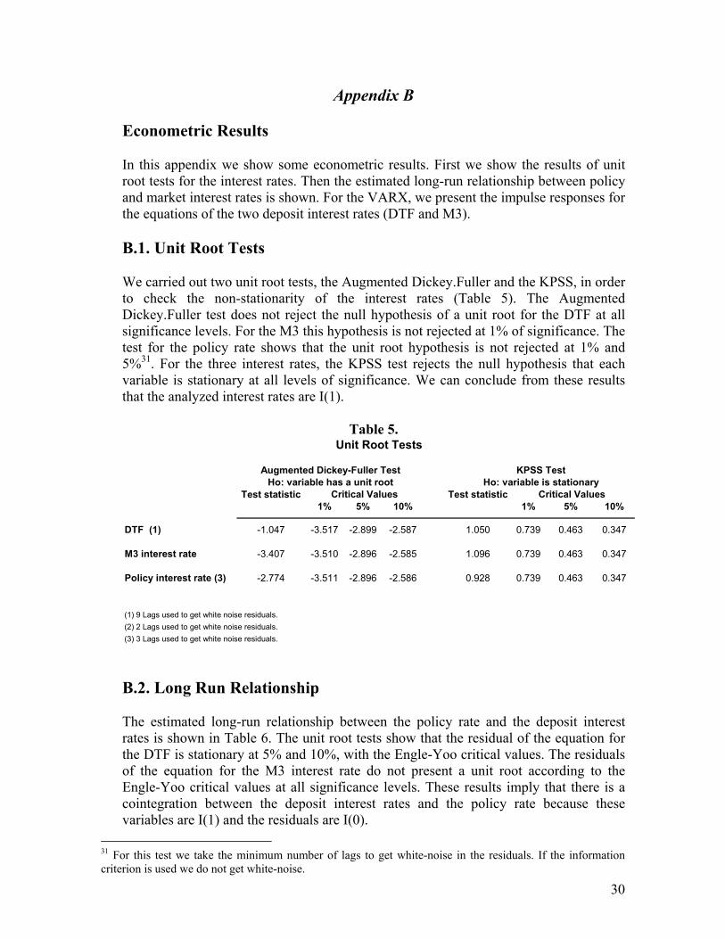
In this appendix we show some econometric results. First we show the results of unit root tests for the interest rates. Then the estimated long-run relationship between policy and market interest rates is shown. For the VARX, we present the impulse responses for the equations of the two deposit interest rates (DTF and M3). B.1. Unit Root Tests We carried out two unit root tests, the Augmented Dickey.Fuller and the KPSS, in order to check the non-stationarity of the interest rates (Table 5). The Augmented Dickey.Fuller test does not reject the null hypothesis of a unit root for the DTF at all significance levels. For the M3 this hypothesis is not rejected at 1% of significance. The test for the policy rate shows that the unit root hypothesis is not rejected at 1% and 5%31. For the three interest rates, the KPSS test rejects the null hypothesis that each variable is stationary at all levels of significance. We can conclude from these results that the analyzed interest rates are I(1).
Table 5.
Test statistic Test statistic1% 5% 10% 1% 5% 10%
DTF (1) -1.047 -3.517 -2.899 -2.587 1.050 0.739 0.463 0.347
M3 interest rate -3.407 -3.510 -2.896 -2.585 1.096 0.739 0.463 0.347
Policy interest rate (3) -2.774 -3.511 -2.896 -2.586 0.928 0.739 0.463 0.347
(1) 9 Lags used to get white noise residuals. (2) 2 Lags used to get white noise residuals. (3) 3 Lags used to get white noise residuals.
Critical Values Critical Values
Unit Root Tests
Augmented Dickey-Fuller Test KPSS TestHo: variable has a unit root Ho: variable is stationary
B.2. Long Run Relationship The estimated long-run relationship between the policy rate and the deposit interest rates is shown in Table 6. The unit root tests show that the residual of the equation for the DTF is stationary at 5% and 10%, with the Engle-Yoo critical values. The residuals of the equation for the M3 interest rate do not present a unit root according to the Engle-Yoo critical values at all significance levels. These results imply that there is a cointegration between the deposit interest rates and the policy rate because these variables are I(1) and the residuals are I(0).
31 For this test we take the minimum number of lags to get white-noise in the residuals. If the information criterion is used we do not get white-noise.

31
Table 6.
DTF (1) M3 (2)
Constant 1.132 -0.777980(0.345) (0.271)
Policy Rate 1.003 0.822(0.037) (0.029)
Test Statistic* -2.575 -3.075
1% 5% 10%2.60 1.95 1.61
* Ho: existence of a unit root** Critical values for a sample of 100 observations and non-constant(1) 3 Lags used in the residual test to get white noise(2) Lags=3 used in the residual test to get white noise
Long Run Equations
Engle Yoo Critical Values**
Dependent Variables
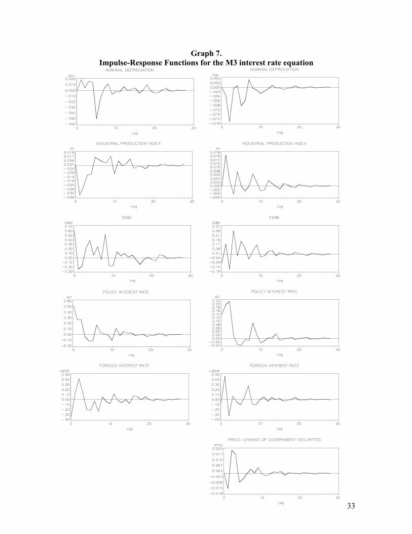
B.3. Impulse-Response Functions The impulse-response functions for the DTF equation in the VARX are shown in Graph 6, including and not the price change of the Government securities. Graph 7 shows the impulse-response functions for the M3 interest rate equation with and without the price change of the public bonds.

32
Graph 6. Impulse-Response Functions for the DTF equation
33
Graph 7. Impulse-Response Functions for the M3 interest rate equation

34
Appendix C
A Small Macroeconomic Model with a Banking Sector
To perform the simulations presented in section 6, the following model of a small, open economy was used. It assumes imperfect capital mobility, backward-looking expectations of inflation and depreciation, and includes a simple version of the banking sector model developed in section 4. The basic setting is an ad-hoc system of an open-economy Phillips Curve, an open-economy IS equation and a balance of payments equation. In the long run the PPP and UIP conditions are met, but in the short run there may movements in the real exchange rate explained by the short-run price stickiness, and there may be deviations from the UIP condition because of the assumption of imperfect capital mobility. The latter is compatible with the existence of a demand for bank loans and a supply of bank deposits, which are imperfect substitutes of foreign bank loans and deposits, respectively. Phillips Curve:
tttoett qqy εααππ +−++= )(
_
1 (A6) Inflation depends on inflation expectations, the output gap and the deviations of the real exchange rate (RER) from its PPP long run level. If the currency is undervalued, the RER is above its long run level and inflation goes up as part of the adjustment of the RER toward its long run equilibrium. Inflation expectations are formed in the beginning of each period. εt is a price shock. IS Curve:
ttet
Dttot qqriyy µδπδδ +−+−−+= − )()(
_
2
_
11 (A7) Dti is the nominal domestic market (deposit) interest rate.32 It is assumed that banks´
interest rates are the relevant prices in the transmission mechanism.33 δo and δ2 > 0. δ1 < 0. µt is an aggregate demand shock. Balance of Payments:
0)1()(^
*^
1*
11*
11
_
=+
−−+
−−+−+− −−−− t
ett
Dt
ett
Dtttto eiifeiifiynxqqnx ζ (A8)
The deviation of the trade balance from its long run equilibrium depends positively on the RER deviation (nxo > 0) and negatively on the output gap (nx1 < 0). One period capital inflows f[.] are assumed. They depend positively on the domestic-external
32 The lending rate could be included. However, since constant operational marginal costs are assumed for banks, the inclusion of deposit rates is equivalent. The distinction would be important if the credit channel were relevant feature of the model economy as in Bernanke and Blinder (1992). 33 To be consistent with the assumption of imperfect substitution between foreign and domestic loans and deposits, the foreign interest rate gap should also be included in the equation. We do not do so for simplicity.
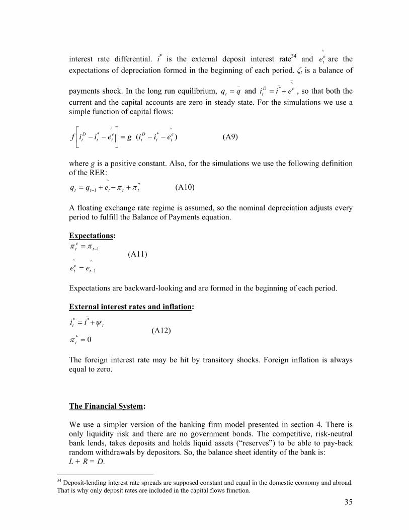
35
interest rate differential. i* is the external deposit interest rate34 and ^ete are the
expectations of depreciation formed in the beginning of each period. ζt is a balance of
payments shock. In the long run equilibrium, _qqt = and
_^_
* eDt eii += , so that both the
current and the capital accounts are zero in steady state. For the simulations we use a simple function of capital flows:
)(^
*^
* ett
Dt
ett
Dt eiigeiif −−=
−− (A9)
where g is a positive constant. Also, for the simulations we use the following definition of the RER:
*^
1 ttttt eqq ππ +−+= − (A10) A floating exchange rate regime is assumed, so the nominal depreciation adjusts every period to fulfill the Balance of Payments equation. Expectations:
^
1
^
1
−
−
=
=
tet
tet
ee
ππ (A11)
Expectations are backward-looking and are formed in the beginning of each period. External interest rates and inflation:
0*
_**
=
+=
t
tt ii
π
ψ (A12)
The foreign interest rate may be hit by transitory shocks. Foreign inflation is always equal to zero. The Financial System: We use a simpler version of the banking firm model presented in section 4. There is only liquidity risk and there are no government bonds. The competitive, risk-neutral bank lends, takes deposits and holds liquid assets (“reserves”) to be able to pay-back random withdrawals by depositors. So, the balance sheet identity of the bank is: L + R = D.
34 Deposit-lending interest rate spreads are supposed constant and equal in the domestic economy and abroad. That is why only deposit rates are included in the capital flows function.

36
Let x~ be the fraction of total deposits, D, that is withdrawn. x~ is a random variable uniformly distributed between 0 and 1. Let ρ the fraction of total deposits that the bank chooses to hold as reserves. If total withdrawals exceed reserves, the bank must borrow the shortfall from the Central Bank at (real) interest rate rp, which is the policy rate. Hence, the expected cost of the funds borrowed from the central bank is:
1 2(1 )[ (0, ( )] ( )2p p pr E Max D x r D x dx r D
ρ
ρρ ρ −
− = − =
∫% % % and the optimization problem
of the bank is: 2
,
(1 )(1 ) (1 )2L D pD
Max r D r D r D mDρ
ρρ ρ −
− − − − −
where rL and rD are real interest rates on loans and deposits, respectively, and m is a constant marginal operational cost incurred on loans. Fist order conditions:
(1 )1 2
(1 )
pDL
L p
rrr m
r r m
ρρ
ρ
−= + +
−
= − +
From these two equations we obtain the optimal fraction of reserves as a function of the deposit and policy interest rates:
21 D
p
rr
ρ = − (A13)
which indicates that the optimal reserve fraction increases with the cost of Central Bank liquidity (the cost of not having reserves) and decreases with the market interest rates (opportunity cost of holding reserves). An interesting implication of equation (A13) is that the relationship between deposit and policy rates is not “one for one”:
2(1 )2
pD
rr
ρ−= (A14)
Actually, in the absence of other risks and costs, in this model deposit interest rates are below policy rates. Also, as it is apparent from equation (A14), if the reserve fraction does not vary too much, the difference between the market and policy rates will move with the level of the policy rate. This is an example of the rather complex relationship that may exist between policy and market rates.

37
To introduce the equilibrium in the deposit and loan markets in the macroeconomic model, we express the balance-sheet constraint in terms of deviations from the steady state:
_ _ _ _
( ) ( ) ( )t t t tD D L L D Dρ ρ− = − + − which implies:
_ _ _ _
( )(1 ) ( ) ( )t t t tD D L L Dρ ρ ρ− − = − + − (A15) Let the following functions represent the deviations of the demand for loans and the supply of deposits from their respective steady state values:
tett
Dtot yeiiDD 1
^*
_)( ωω +−−=− (A16)
tett
Dtot yeiiLL 1
^*
_)( λλ +−−=− (A17)
In the latter equation, lending-deposit interest rate spreads are assumed to be equal in the economy and abroad. Together with the definition of the real interest rates (Fisher equations) e
tp
tp
t ir π−= and et
Dt
Dt ir π−= , equations (A13) and (A15)-(A.17) define the equilibrium deposit rates in
terms of the policy rate and macro variables like the output gap, the expectations of depreciation and inflation, and foreign interest rates. Monetary Policy Rule: It is assumed that the Central Bank knows the structure and parameters of the economy, including the behavior of banks and the features of the financial markets. With that knowledge, the Central Bank sets the policy rates, so that the πTARGET = 0 is met every period (“strict” inflation targeter). Macroeconomic equilibrium: The deposit rate that results from the equilibrium in the loans and deposit markets, and the monetary policy rule are then included in the macro model (A6)-(A12), to yield the equilibrium inflation, nominal depreciation and output gap in terms of the exogenous variables. The order of events in the model economy is as follows: (i) Agents form expectations. (ii) Shocks occur. (iii) The Central Bank reacts to the shocks. (iv) Endogenous variables (market interest rates, the output gap, nominal depreciation and inflation) are determined. In steady state, inflation is on target, and nominal depreciation and inflation expectations equal inflation. The output gap, the trade balance and capital flows are zero. The RER is at its long-run PPP level and domestic loan and deposit interest rates fulfill the UIP condition. The reserves ratio, ρ, is at its long run level which, given UIP,
38
is determined by the external interest rates (see the first order conditions of the bank´s problem above). The steady state policy rate is obtained from equation (A14), given the steady state values of ρ and rD. Parameters used in the Simulation: Long run levels of interest and real exchange rates: _q = 0
_*
_rr = = 0.025
Parameters of the macroeconomic equations: αo = 0.2 α1 = 0.04 δo = 0.7 δ1 = -0.1 δ2 = 0.02 nxo = 0.1 nx1 = 0.2 g = 1 Parameters of the Financial System: ω0 = 1 ω1 = 1 λo = 1 λ1 = 1
_D = 1 _ρ = 0.025

39
Appendix D
The description of the variables used in the econometric exercise is given in the following table.
Table 7.
Variable Definition Sample Frequency Source DDTF Difference of the nominal 90-day
deposit interest rate June 1999 August 2006
Monthly Banco de la República
DM3 (1) Difference of the nominal average deposit interest rate
June 1999 August 2006
Monthly Banco de la República
DPOLICY Difference of the nominal policy interest rate “Subasta de Expansión”
June 1999 August 2006
Monthly Banco de la República
DDEPRECIATION Difference of the nominal annualized quarterly depreciation
June 1999 August 2006
Monthly Banco de la República
DINFLATION Difference of the consumer annual inflation
June 1999 August 2006
Monthly DANE
DIPI Logarithmic difference of the deseasonal industrial production index
June 1999 August 2006
Monthly DANE Authors
DITES Logarithmic difference of the I-TES (Price Index of a representative bundle of fixed rate peso denominated Government Bonds)
December 2001 August 2006
Monthly Corfinsura SuValor
DEMBI Logarithmic difference of the EMBI Colombia
June 1999 August 2006
Monthly Bloomberg
DLIBOR (2) Difference of the nominal LIBOR in dollars.
June 1999 August 2006
Monthly Datastream
(1) The M3 interest rate corresponds to the average of the interest rates for different types of deposits (saving accounts, 90-day CDs and 360-day CDs) weighted by their volume. (2) LIBOR (London Interbank Offer Rate) is the interest rate for 3-month deposits in dollars.