Embed Size (px)
Citation preview
Institute of Actuaries of Australia ABN 69 000 423 656
Level 2, 50 Carrington Street, Sydney NSW Australia 2000
t +61 (0) 2 9233 3466 f +61 (0) 2 9233 3446
e [email protected] w www.actuaries.asn.au
Interest Rates and Inflation in
Property/Casualty Insurance
Prepared by the Working Group of the German Association of Actuaries
Presented to the Actuaries Institute
ASTIN, AFIR/ERM and IACA Colloquia
23-27 August 2015
Sydney
This paper has been prepared for the Actuaries Institute 2015 ASTIN, AFIR/ERM and IACA Colloquia.
The Institute’s Council wishes it to be understood that opinions put forward herein are not necessarily those of the
Institute and the Council is not responsible for those opinions.
German Association of Actuaries
The Institute will ensure that all reproductions of the paper acknowledge the
author(s) and include the above copyright statement.
1
Report on the findings of the German Association of Actuaries e.V.
Interest Rates and Inflation in Property / Casualty Insurance
Cologne, 24 September 2014
2
Preamble
This study has been written by the working group "Interest and Inflation in Property Insurance“. This working group1 originates from the DAV working group on claims reserving but was staffed also with members from other specialist areas in order to be able to consider wider issues than reserving.
The aim of this study is to investigate the effects of interest and inflation on property/casualty insurance. It collates and prepares background information on economic connections, financial mathematics and legal aspects relating to the topic. Using these as a basis it analyses and discussed a variety of questions concerning claims reserving, pricing and risk modelling. Moreover, possible solutions are developed, tested and presented in the report.
The findings constitute the current state of discussion and the conclusions of the working group. The results of the working group are to be made available to the members of the DAV for information purposes as well as to provide impetus for their own actuarial practice.
The aim of this report is to stimulate discussion and, as a consequence, to develop further the ideas and approaches presented. Hence, with this in mind, the working group welcomes feedback.
The report does not constitute a binding position on the part of the DAV and does not purport to contain guidelines for actuarial practice.
The technical scope of this report falls within property/casualty insurance unless any legal or actuarial guidelines from life or health insurance have to take precedence.
The non-life insurance committee of the DAV adopted this report on 24 July 2013.
1 Members of the working group are: Dr. Daniel John (Chair), Mina Averbach, Kristina Baganz, Harald Bredl, Sami Demir, Dr. Heinz-Jürgen Klemmt, Dr. Matthias Land, Philipp Maier, Susanne Plümacher, Dr. Jürgen Reinhart, Karsten Wantia. The translation to an English version was supervised by Prof. Dr. Michael Radtke and Dr. Marcel Wiedemann.
3
Contents
1 Introduction ...................................................................................................................... 7
1.1 A new challenge ....................................................................................................... 7
1.2 Effects of inflation – an initial insight .................................................................. 9
2 Terminology and economic context .......................................................................... 11
2.1 Terminology............................................................................................................. 11
2.1.1 The pace of inflation....................................................................................... 11
2.1.2 The cause of inflation..................................................................................... 12
2.1.3 The characteristics of inflation..................................................................... 17
2.2 Measuring inflation ................................................................................................ 18
2.2.1 Inflation indices ............................................................................................... 18
2.2.2 Market data interest rates ............................................................................ 21
3 Retrospective look at interest rates and inflation.............................................................. 24
3.1 Overview of the historic development of interest rates and the CPI......... 24
3.2 Inflation in historic claims data .......................................................................... 27
3.2.1 Determining inflation from the accident year view ................................ 29
3.2.2 Separation Method ......................................................................................... 33
3.2.3 Comparing claims portfolio inflation with public inflation indices ....... 38
3.3 Including inflation assumptions in the calculation of reserves ................... 42
3.3.1 Calculating reserves adjusted for inflation – Method............................. 42
3.3.2 Example: Consequences of inflation assumptions in the calculation of reserves ........................................................................................................................... 43
3.3.3 Conclusion ........................................................................................................ 44
3.4 Including inflation assumptions in excess of loss rating .............................. 46
4 Future development of interest rate and inflation ............................................................. 51
4.1 Development of deterministic interest scenarios ........................................... 51
4.2 Development of deterministic inflation scenarios .......................................... 52
4.2.1 Inflation forecasting ....................................................................................... 52
4.2.2 Scenario analyses ........................................................................................... 54
4.3 Inflation in stochastic capital market scenarios ............................................. 58
4.4 Stochastic processes to describe economic scenarios .................................. 59
4.4.1 Inflation as a stochastic process ................................................................. 60
4.4.2 Expected future inflation ............................................................................... 67
4.5 Inflation risk in property / casualty insurance ................................................ 68
4
4.5.1 Fundamentals .................................................................................................. 68
4.5.2 Representing inflation risk in internal models ......................................... 69
5 Accounting and legal aspects ........................................................................................... 71
5.1 HGB (German GAAP)............................................................................................. 71
5.1.1 Effects on liabilities......................................................................................... 71
5.1.2 Effects on assets ............................................................................................. 71
5.2 IFRS........................................................................................................................... 72
5.2.1 Effects on liabilities......................................................................................... 72
5.2.2 Effects on assets (IAS 39) ............................................................................ 72
5.3 Solvency II .............................................................................................................. 73
5.4 Practice in companies ........................................................................................... 74
6 Further aspects of interest rate and inflation .................................................................... 76
6.1 Pricing in primary insurance ................................................................................ 76
6.2 Hedging against inflation ..................................................................................... 76
7 Inflation indices.................................................................................................................. 80
7.1 Prices......................................................................................................................... 80
7.1.1 Consumer Price Index (CPI)......................................................................... 80
7.1.2 Harmonised Consumer Price Index (HCPI) .............................................. 81
7.1.3 CPI Transport................................................................................................... 83
7.1.4 CPI Healthcare................................................................................................. 84
7.2 Wages and salaries ................................................................................................ 86
7.2.1 Index of wages and salaries from collectively agreed earnings & national accounts........................................................................................................... 86
7.2.2 Index of wages and salaries for collectively agreed earnings & national accounts – Transport (trade in, maintenance and repair of motor vehicles)........................................................................................................................... 87
7.2.3 Index of wages and salaries for collectively agreed earnings & national accounts - healthcare ................................................................................... 88
7.2.4 Index of wages and salaries for collectively agreed earnings & national accounts – social care (with homes) ........................................................ 89
7.3 GDP Deflator ........................................................................................................... 90
7.4 MEDI (medical expenses index) ......................................................................... 91
7.5 Construction price index for residential property ........................................... 91
8 Bibliography....................................................................................................................... 93

5

6
7
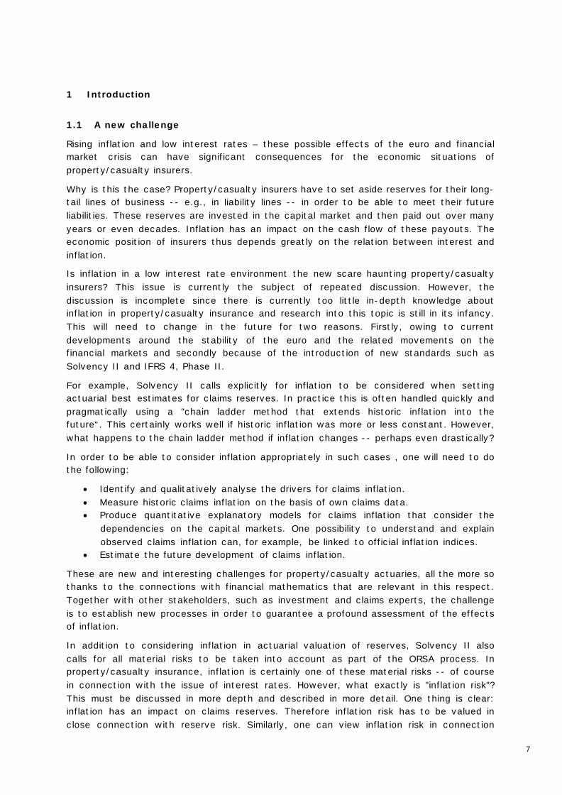
1 Introduction
1.1 A new challenge
Rising inflation and low interest rates – these possible effects of the euro and financial market crisis can have significant consequences for the economic situations of property/casualty insurers.
Why is this the case? Property/casualty insurers have to set aside reserves for their long-tail lines of business -- e.g., in liability lines -- in order to be able to meet their future liabilities. These reserves are invested in the capital market and then paid out over many years or even decades. Inflation has an impact on the cash flow of these payouts. The economic position of insurers thus depends greatly on the relation between interest and inflation.
Is inflation in a low interest rate environment the new scare haunting property/casualty insurers? This issue is currently the subject of repeated discussion. However, the discussion is incomplete since there is currently too little in-depth knowledge about inflation in property/casualty insurance and research into this topic is still in its infancy. This will need to change in the future for two reasons. Firstly, owing to current developments around the stability of the euro and the related movements on the financial markets and secondly because of the introduction of new standards such as Solvency II and IFRS 4, Phase II.
For example, Solvency II calls explicitly for inflation to be considered when setting actuarial best estimates for claims reserves. In practice this is often handled quickly and pragmatically using a "chain ladder method that extends historic inflation into the future“. This certainly works well if historic inflation was more or less constant. However, what happens to the chain ladder method if inflation changes -- perhaps even drastically?
In order to be able to consider inflation appropriately in such cases , one will need to do the following:
• Identify and qualitatively analyse the drivers for claims inflation. • Measure historic claims inflation on the basis of own claims data. • Produce quantitative explanatory models for claims inflation that consider the
dependencies on the capital markets. One possibility to understand and explain observed claims inflation can, for example, be linked to official inflation indices.
• Estimate the future development of claims inflation.
These are new and interesting challenges for property/casualty actuaries, all the more so thanks to the connections with financial mathematics that are relevant in this respect. Together with other stakeholders, such as investment and claims experts, the challenge is to establish new processes in order to guarantee a profound assessment of the effects of inflation.
In addition to considering inflation in actuarial valuation of reserves, Solvency II also calls for all material risks to be taken into account as part of the ORSA process. In property/casualty insurance, inflation is certainly one of these material risks -- of course in connection with the issue of interest rates. However, what exactly is "inflation risk"? This must be discussed in more depth and described in more detail. One thing is clear: inflation has an impact on claims reserves. Therefore inflation risk has to be valued in close connection with reserve risk. Similarly, one can view inflation risk in connection

8
with premium risk. This consideration formed the basis for the definition of "inflation risk" in this study. Alongside the issue of the definition of inflation risk the issue of modelling and measuring this risk is particularly interesting. What should stochastic models for representing inflation risk look like? How can they be calibrated and validated? And how can they be implemented as part of an internal model?
These are all issues that actuaries in property/casualty insurance are going to have to consider in future.
Hence, the aim of this study is to ask precisely these questions and lay the foundations for being able to answer them.
We do not see this work as a "textbook" that collates all techniques and methods surrounding the topic of inflation and interest in property/casualty insurance.
Of course we present theoretical approaches and methods from literature and practice. However, these are limited since the topic is obviously still "in its infancy".
Our primary aim is therefore to encourage more intensive consideration of the issues of inflation and interest rates and to nurture the development of further ideas. It is against this backdrop that we present our own ideas, methods and results.
We hope to generate lively -- perhaps even controversial -- discussion of this fascinating topic.

9
1.2 Effects of inflation – an initial insight
The consequences of inflation in property/casualty insurance can be significant. This is demonstrated by the following example:
The table in Figure 1: Cover shortfall or redundancy of reserves depending on run-off duration and "misjudgement of inflation"", shows, with thanks to Dowling & Partners2), the cover shortfall or redundancy of reserves depending on the duration of the run-off and the "misjudgement" of inflation. Misjudgement of inflation means the deviation between future inflation and the inflation actually observed during the period in question, i.e., the inflation implicitly present in the triangles. The assumption is that the projected cash flow does not include this deviation from implicit inflation and there is thus a difference to the actually realised cash flow that affects income.
Results are shown as a percentage of the nominal original reserve. A positive prefix represents a gain and a negative one a loss.
The table shows, for example, that in a “long-tail“ segment with an average run-off duration of 5 years and with inflation being “misjudged” by -2% the nominal reserve is overestimated at 9.6%. This equates to a profit of the same amount being generated over the whole run-off period. If, in this example, one assumes implicit (present in the triangles) average inflation of 1.5%, this means that, in this case, a deflationary environment is prevailing (median deflation = 2% - 1.5% = 0.5%).
Inflation misjudgement Segment
-3% -2% -1% 1% 2% 3% 4% 5%
Ave
rage
run
-off
dur
atio
n in
yea
rs
0,5 1,5% 1,0% 0,5% -0,5% -1,0% -1,5% -2,0% -2,5%
1,0 3,0% 2,0% 1,0% -1,0% -2,0% -3,0% -4,0% -5,0% "Short-Tail"
1,5 4,5% 3,0% 1,5% -1,5% -3,0% -4,5% -6,1% -7,6%
2,0 5,9% 4,0% 2,0% -2,0% -4,0% -6,1% -8,2% -10,3%
2,5 7,3% 4,9% 2,5% -2,5% -5,1% -7,7% -10,3% -13,0% "Medium-Tail"
3,0 8,7% 5,9% 3,0% -3,0% -6,1% -9,3% -12,5% -15,8%
3,5 10,1% 6,8% 3,5% -3,5% -7,2%
-10,9% -14,7% -18,6%
4,0 11,5% 7,8% 3,9% -4,1% -8,2%
-12,6% -17,0% -21,6% "Long-Tail"
4,5 12,8% 8,7% 4,4% -4,6% -9,3%
-14,2% -19,3% -24,6%
5,0 14,1% 9,6% 4,9% -5,1% -10,4%
-15,9% -21,7% -27,6%
Figure 1: Cover shortfall or redundancy of reserves depending on run-off duration and "misjudgement of inflation"
2 IBNR weekly (#29, Vol. XVI – Page 3) July 2009

10
This table clearly demonstrates how significant the lever of inflation can be for the amount of reserves. Especially in long-tail lines of business, estimating inflation appropriately is thus crucial for the economic success of an insurer.
11
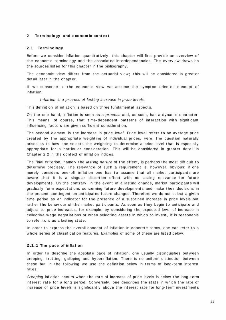
2 Terminology and economic context
2.1 Terminology
Before we consider inflation quantitatively, this chapter will first provide an overview of the economic terminology and the associated interdependencies. This overview draws on the sources listed for this chapter in the bibliography.
The economic view differs from the actuarial view; this will be considered in greater detail later in the chapter.
If we subscribe to the economic view we assume the symptom-oriented concept of inflation:
Inflation is a process of lasting increase in price levels.
This definition of inflation is based on three fundamental aspects.
On the one hand, inflation is seen as a process and, as such, has a dynamic character. This means, of course, that time-dependent patterns of interaction with significant influencing factors are given sufficient consideration.
The second element is the increase in price level. Price level refers to an average price created by the appropriate weighting of individual prices. Here, the question naturally arises as to how one selects the weighting to determine a price level that is especially appropriate for a particular consideration. This will be considered in greater detail in Chapter 2.2 in the context of inflation indices.
The final criterion, namely the lasting nature of the effect, is perhaps the most difficult to determine precisely. The relevance of such a requirement is, however, obvious: if one merely considers one-off inflation one has to assume that all market participants are aware that it is a singular distortion effect with no lasting relevance for future developments. On the contrary, in the event of a lasting change, market participants will gradually form expectations concerning future developments and make their decisions in the present contingent on anticipated future changes. Therefore we do not select a given time period as an indicator for the presence of a sustained increase in price levels but rather the behaviour of the market participants. As soon as they begin to anticipate and adjust to price increases, for example, by considering the expected level of increase in collective wage negotiations or when selecting assets in which to invest, it is reasonable to refer to it as a lasting state.
In order to express the overall concept of inflation in concrete terms, one can refer to a whole series of classification features. Examples of some of these are listed below.
2.1.1 The pace of inflation
In order to describe the absolute pace of inflation, one usually distinguishes between creeping, trotting, galloping and hyperinflation. There is no uniform distinction between these but in the following we use the definition below in terms of long-term interest rates:
Creeping inflation occurs when the rate of increase of price levels is below the long-term interest rate for a long period. Conversely, one describes the state in which the rate of increase of price levels is significantly above the interest rate for long-term investments
12
as galloping inflation. The transition from creeping to galloping inflation is described as trotting inflation.
One acknowledged criterion for hyperinflation is a rate of increase of price levels of at least 100% per annum over a period of several years.
Alongside the absolute pace the pace of the change of inflationary developments also plays a crucial role when considering inflation. Inflation can be stable (constant) or accelerating or decelerating.
2.1.2 The cause of inflation
In order to consider the economic causes a certain knowledge of the theory of macro-economic models is required. Without going into too much detail we will provide a very puristic overview of the Keynesian approach to explaining variations in price levels. For other approaches and further developments readers are referred to the relevant literature. The sources forming the basis for these explanations can be found in the bibliography.
The predominant feature is the premise of a world that can be viewed exclusively empirically. Thus all market players are inevitably in a state whereby they have imperfect information. Only by means of this assumption can disequilibria arise from the sequence of economic processes and disequilibria generated by external distortions exist permanetly. This approach is denoted as multi-causal because it allows for autonomous shifts in supply and demand as well as in the money supply as the cause of changes in price level.
The Keynesian money market is determined by the nominal demand for money and the nominal supply of money . In equilibrium the following condition applies:
.
Thus the supply of money corresponds exactly to the nominal amount of money available. The demand for money is modelled using cash management, thus simulating the fact that market participants keep some of their money in a form that does not earn interest but is instead readily available. This behaviour is known as the liquidity preference. The reasons for maintaining liquidity are, on the one hand, the desire to protect against unforeseen expenditure or to bridge periods between earning and expenditure or buying and selling (transactions motive) and, on the other hand, speculation, i.e., the expectation of being able to take advantage of short-term favourable investment opportunities (speculative motive). It is therefore appropriate to state that rising interest rates reduce the speculative motive. If denotes the money held for speculative purposes and the interest rate then the following holds:
.
According to Keynes, the nominal demand for money arises from the sum of monies held for transactions and speculative purposes:
,
whereby is the cash management coefficient, the price level and the volume of production.
The market for goods regulates itself via the condition of equilibrium which states that the real supply of goods corresponds to the real demand for goods :
13
.
Similar to the money market, the supply of goods corresponds exactly to the volume of production The demand for goods consists of real demand for consumer goods , real demand for investment and real tax expenditure . Therefore
,
with being real tax revenue and a function of net income . One requires that the demand for consumer goods rises if net income rises, the demand for investment I, which is usually credit constrained, falls if the interest rate rises:
and .
On the labour market, equilibrium is only possible in the event of full employment, i.e., if the supply of labour is equal to the demand for labour . Equilibrium also exists if there is an excess supply of labour. The supply of labour may be a function of nominal wage , which increases the higher that becomes but two crucial constraints apply. If labour is too poorly remunerated the employee will no longer offer his labour. In concrete terms this threshold is known as the prevailing nominal wage . Hence
in case .
Moreover, there must be a ceiling for the amount of labour offered which cannot be expanded by means of further wage increases:
in case ,
with being the wage threshold up to which the supply of labour is stillelastic.
Demand for labour depends only on the real wage level and will increase if this falls:
with .
Let us now turn our attention back to inflation. In line with the reasons for how inflation arises we distinguish between the following types of inflation:
2.1.2.1 Monetary inflation
Monetary inflation arises when additional money is injected into the money market. The resulting excess supply means that banks initially reduce interest rates which, in line with the theory of liquidity preference, causes more money to be held for speculative purposes. This encourages investment, in turn stimulating the real demand for goods. Disequilibrium arises when demand for goods exceeds supply. This leads to price increase which in turn results in real wages decreasing given a nominal wage. Now, since cheaper labour is now available and money is available for speculation, factory owners expand production capacity. Higher production reduces the gap in supply and price levels begin to stabilise. Simultaneously, this increase in production via transaction money increases the demand for money on the money market, which then has a counter effect on the excess supply of money. Interest rates increase again, thus dampening demand for goods. This new state of equilibrium depends strongly on the labour market situation.
Let us first of all consider underemployment. In this model, underemployment means that nominal wages remain constant when production capacity is expanded by increasing the workforce. Now an increase in the money supply as described above leads to an
14
increase in price levels. In combination with constant nominal wages this results in real wages actually decreasing and a real expansion of production capacity. Thanks to higher production and greater demand for money the additional money supply is only partially reflected in an increase in price levels. It is, as a result, both disproportionately low compared to the increase in the money supply and of minimal extent.
Now let us assume we have elasticity of full employment. Unlike with underemployment, nominal wages increase with the demand for labour. Despite a rise in price levels, real wages hardly fall, production subsequently increases marginally and the new equilibrium only leads to a small increase in demand for money. All in all, we have a similar picture to our previous case though here a larger proportion of the increase in the money supply results in an increase in price levels. The increase is still disproportionately low but is already moderate.
If we finally consider non-elasticity of full employment we see an increase in price levels that is proportionate to the increase in the money supply. Logically, the inability to expand production is caused by the lack of an increase in the labour supply.
Monetary policy strategies to counter monetary inflation include restricting, or making more expensive, the flow of central bank money into the commercial banking system. This can be done by raising minimum reserves, i.e., the minimum level of deposits that commercial banks have to maintain at the central bank. This has the effect of withdrawing liquidity from the commercial banks, as it is then no longer available for lending. On a similar note, central banks have other monetary policy instruments at their disposal with which to influence interest rates and liquidity, such as standing facilities and open market operations.
2.1.2.2 Demand-Pull Inflation
Demand-pull inflation is triggered by an increase in autonomous demand in the market, for example, in the form of a heightened appetite for investment or increased consumption but not by an increase in demand arising from an increase in the money supply.
In principle, the consequences of the demand-pull inflation are the same as outlined in the paragraphs above. In the event of underemployment or of elasticity of full employment, companies are induced to deploy more labour and hence increase production. Unlike in the above, however, the money supply remains unchanged. Increased demand is now accompanied by higher interest rates, thus reducing the money available for speculation. Since the money supply remains constant the money available for transactions increases. In other words, additional funds are activated that are available for consumption, thus creating further demand. The result is an increase in price levels.
In the case of non-elasticity of full employment, interest rates rise, too, as a result of increased demand, thus reducing demand that is sensitive to interest rates. Unlike in the earlier scenario, there are no positive impulses for investment. In total, this scenario does give rise to an increase in price levels, but much less so.

15
Figure 23: This diagram shows in simplified form the dynamic dependencies in play in the process of demand-pull inflation. If demand exceeds supply this induces factories to
expand production capacities. Employment and wages rise and drive demand higher.
Effective policy measures available to counter demand-pull inflation include, for example, targeted tax increases (taxing profits, which dampens investment; increasing value-added tax, thus reducing consumer spending, etc.) and artificial interest rate increases by means of central bank policy instruments.
2.1.2.3 Supply-Push (Cost-Push) Inflation
In the Keynesian model, supply-push or cost-push inflation occurs when prices rise as a result of a fall in supply. A fall in supply can be triggered either by an increase in costs or profits in an environment where there is little or no competition.
An increase in production costs such as higher labour costs, energy costs or taxation (see Fig. 3) means that the marginal costs of production increase. If one assumes that companies and manufacturers in the market behave in such a way as to maximise their profit then, if price levels remain unchanged, this will result in a drop in production. This will, in turn, lead to a gap in the supply of goods, driving prices upwards at the expense of demand. These higher prices will induce manufacturers to expand production until stability is achieved. The new equilibrium will then mean higher prices and lower production. In this case we refer to cost-push inflation.
3 Drawn from [BWLhelfer / Business Administration Explained]
16
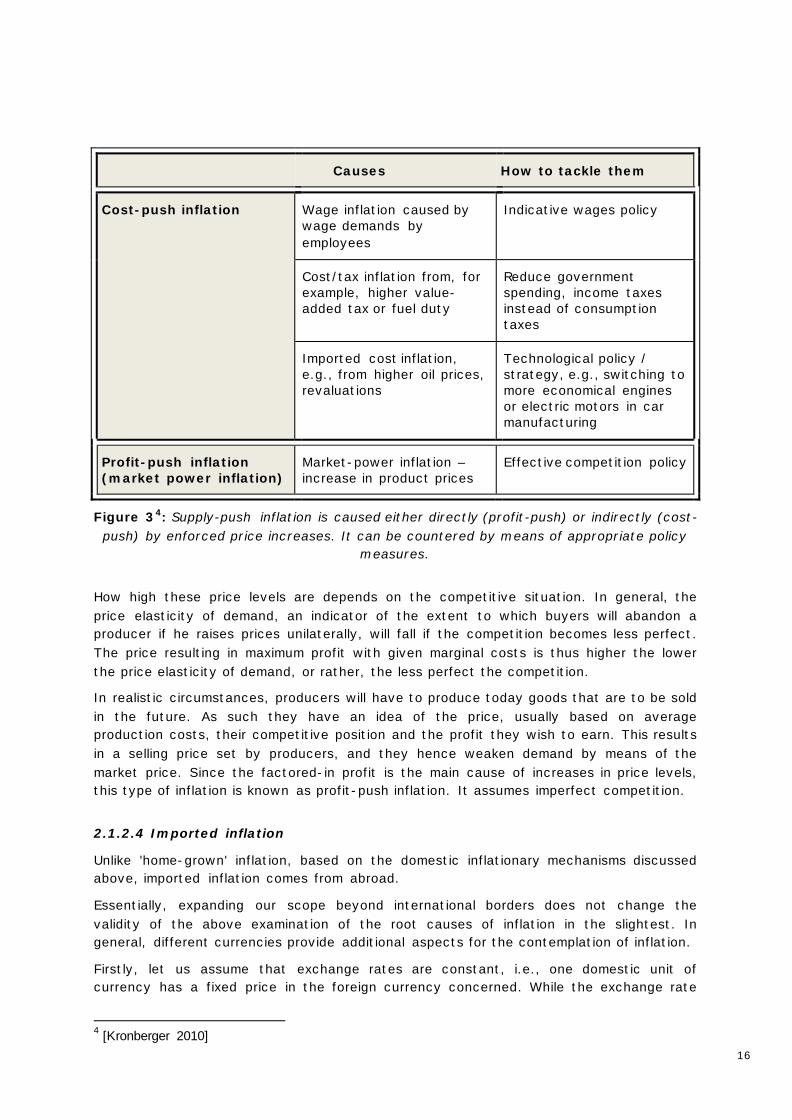
Figure 34: Supply-push inflation is caused either directly (profit-push) or indirectly (cost-push) by enforced price increases. It can be countered by means of appropriate policy
measures.
How high these price levels are depends on the competitive situation. In general, the price elasticity of demand, an indicator of the extent to which buyers will abandon a producer if he raises prices unilaterally, will fall if the competition becomes less perfect. The price resulting in maximum profit with given marginal costs is thus higher the lower the price elasticity of demand, or rather, the less perfect the competition.
In realistic circumstances, producers will have to produce today goods that are to be sold in the future. As such they have an idea of the price, usually based on average production costs, their competitive position and the profit they wish to earn. This results in a selling price set by producers, and they hence weaken demand by means of the market price. Since the factored-in profit is the main cause of increases in price levels, this type of inflation is known as profit-push inflation. It assumes imperfect competition.
2.1.2.4 Imported inflation
Unlike 'home-grown' inflation, based on the domestic inflationary mechanisms discussed above, imported inflation comes from abroad.
Essentially, expanding our scope beyond international borders does not change the validity of the above examination of the root causes of inflation in the slightest. In general, different currencies provide additional aspects for the contemplation of inflation.
Firstly, let us assume that exchange rates are constant, i.e., one domestic unit of currency has a fixed price in the foreign currency concerned. While the exchange rate
4 [Kronberger 2010]
Causes How to tackle them
Cost-push inflation Wage inflation caused by wage demands by employees
Indicative wages policy
Cost/tax inflation from, for example, higher value-added tax or fuel duty
Reduce government spending, income taxes instead of consumption taxes
Imported cost inflation, e.g., from higher oil prices, revaluations
Technological policy / strategy, e.g., switching to more economical engines or electric motors in car manufacturing
Profit-push inflation (market power inflation)
Market-power inflation – increase in product prices
Effective competition policy
17
and its inverse basically depend on supply and demand, in the case of fixed exchange rates the central bank artificially intervenes. It buys up surplus foreign currency supply in return for national currency or offsets surplus demand for foreign currency by accepting national currency.
If prices abroad rise while remaining stable at home, foreign markets demand more goods as they have become cheaper in relative terms because of the inflation gap. This means the export value of the domestic market in the domestic currency increases. Simultaneously domestic markets demand fewer imported goods, which have now become more expensive. The difference between export and import value, the so-called trade balance, increases. If exports exceed imports then the supply of foreign exchange exceeds demand. This excess supply is offset by the central bank selling domestic currency, thus increasing the money supply and sparking the process of monetary inflation. This development is dampened by the capital markets however. Higher nominal interest rates abroad make investments in foreign exchange more attractive for domestic investors and, conversely, the domestic capital market becomes less attractive for foreign investors. The capital market flow thus runs counter to the flow of goods. Alongside the increase in the money supply, a rise in demand also leads to demand-pull inflation as a result of higher exports. Since imported goods have become more expensive and they are used wholly or partly in the production process the resulting rise in price leads to cost-push inflation.
Floating exchange rates rule out money supply inflows from abroad since the central bank does not intervene in the domestic money market by means of corrective foreign exchange measures. In the event of an inflation gap between domestic and foreign market this flexible adjustment has the effect of revaluing the domestic currency compared to the foreign currency, thus levelling the gap. Hence there is no incentive for foreign markets to increase their demand for domestic products, meaning that imports are not impaired. Provided that this adjustment works perfectly, imported inflation can be avoided.
2.1.3 The characteristics of inflation
As mentioned several times already inflation can be controlled by politically-steered countermeasures. It may well be that inflation is not openly reflected in price level statistics but is prevented, for example, by a price freeze. This is known as repressed or suppressed inflation.
If the increase in price level affects all price ratios we refer to pure inflation, if price ratios change then we refer to impure inflation.
In the context of the focus of this study, property/casualty insurance, two further concepts are significant: implicit inflation and superimposed inflation.
Implicit inflation is the inflation contained in the run-off triangles in claims payments. If the run-off triangles are not adjusted for inflation and the chain-ladder method is used then this implicit inflation will be perpetuated into the future.
When one looks more closely at the problem of inflation of insurance claims one frequently represents claims inflation as the sum of consumer price inflation and an additional component, so-called superimposed inflation. This represents everything that goes beyond existing basis inflation, is LoB-specific and typically consists of various factors. In the case of insurance claims, this could be inflationary developments in relevant industries such as in medical care; wage increases in important industries, for
18
example, the remuneration of lawyers; new developments or changes in legal opinion concerning, for example, the level of damages, as well as social changes, for example an increased sense of entitlement among injured parties5. It must be noted that superimposed inflation is defined as relative to consumer price inflation and not, as is often observed in informed discussion, relative to implicit inflation.
2.2 Measuring inflation
The sheer variety of possibilities of classifying inflation makes it clear there is no such thing as the type of inflation in the actual sense of the word. Therefore it is not surprising that the data used as a basis has considerable influence on how inflation is measured. Depending on the context being observed, the selection of individual positions and their weightings are aligned with one another in order to determine a price level, an index, that is as relevant as possible. Inflation is then defined as the change in this index compared to the previous period by means of
or .
In practice one can refer to the many official inflation indices available. Common sources include Eurostat, Destatis and the like. We will consider some key indices in more depth below.
2.2.1 Inflation indices
In Germany prices are captured in a whole series of price indices. Some of them are listed in Figure 4.
The most common general index is the Consumer Price Index (CPI). This index regularly uses representative random samples to maintain and update pricelists for a wide range of goods and services throughout Germany, using a fixed classification for groups of goods, to determine average prices. A weighting pattern, based on statistical findings relating to the proportion of spending by private households, is used to average these prices for groups of goods to create the CPI. Prices in the CPI are given as percentages compared to a base year that was given a value of 100 points.
Since 1995, on the basis of the CPI, the harmonised consumer price index (HCPI) has been determined. Unlike the CPI, the HCPI for Germany does not take into account spending on gambling, own-use residential property, car tax and car registration fees. Prices are captured throughout Europe but the index is adjusted to reflect specific circumstances in the respective countries. However, the underlying methodology applied is largely comparable throughout Europe.
5 See [Gen Re]

19
General LoB-specific Claims category specific
HCPI
CPI
CPI Transport
Motor vehicles
Operating and Maintenance
CPI Healthcare
Outpatient
Inpatient
Medical equipment
LGI VGR
Automobile sector Trade, maintenance and repair
Social sector
Healthcare
Welfare
LGI Tarif
Automobile sector Trade, maintenance and repair
Social sector
Healthcare
Welfare
GDP
MEDI
Rehab
Care
Building price index Residential buildings
Figure 4: For individual insurance lines of business (LoBs) specific sub-indices of the general inflation indices shown on the left can, under certain circumstances, better reflect the actually
observed claims inflation. If the LoBs are heterogeneous in the claims categories, as is the case with motor liability, then further refinement can show better alignment with the type of claim being
considered.
The LGI wage and salary index is based on data that is collected as part of the quarterly earnings survey. This includes the development of gross wages of almost all employees
20
with the exception of employees without a contract or who are in partial retirement, so-called 1-euro jobs and employees who are employed abroad or whose remuneration is exclusively fee based. Gross earnings are collated into indices according to industry and qualification profile; these indices show earnings development for full-time employees assuming a constant composition of and numbers in the workforce based on the base year 2010. The LGI index is hence a good reference for assessing inflation in personal injury claims using payments for loss of earnings as a basis.
The "LGI Tarifverdienst“ (collectively agreed earnings) index collects data from around 600 selected collective agreements that include at least 75% of employees with collectively agreed salaries. Moreover, the index collects data on employees' collectively agreed earnings as well as information on working hours, the dates the collective agreements were signed and cancelled as well as information on the respective level of the German statutory employee savings schemes known as vermögenswirksame Leistungen. In line with the earnings structure survey from the base year 2006, these are then weighted to form the index.
The LGI VGR index is compiled as part of the national accounts. It comprises the domestic product computation, the input-output account, the financial account, the labour force account, the labour volume account and the capital account.
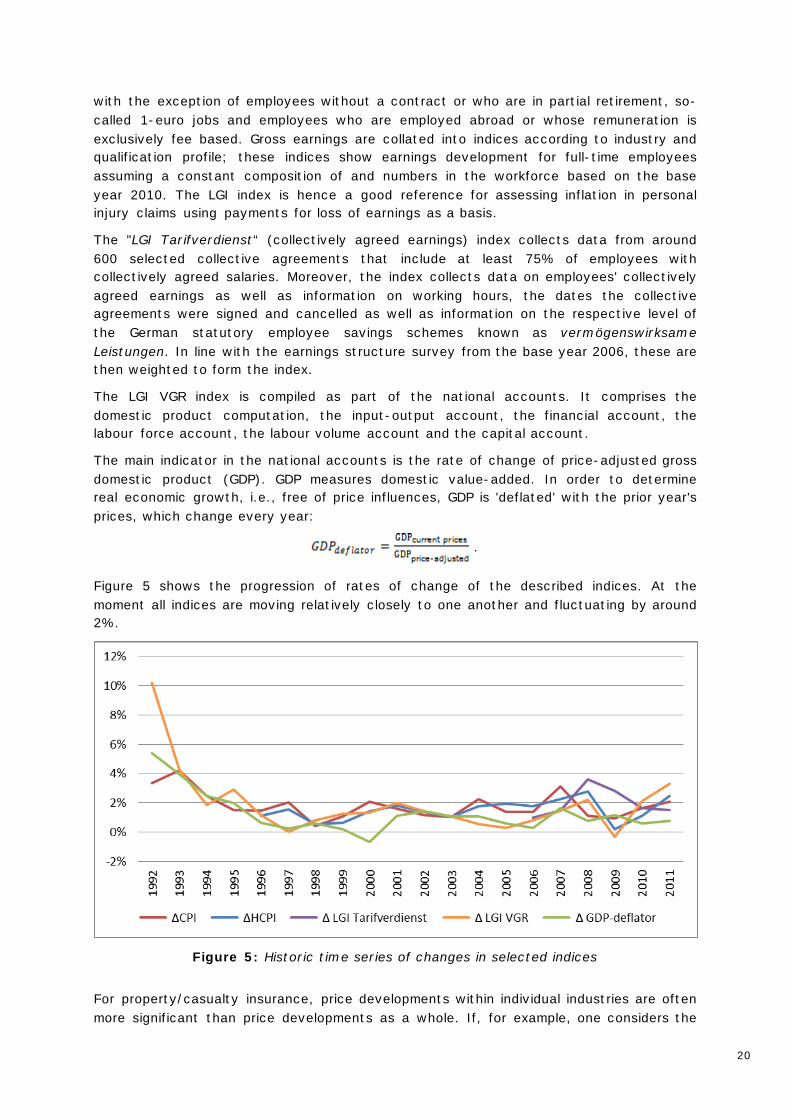
The main indicator in the national accounts is the rate of change of price-adjusted gross domestic product (GDP). GDP measures domestic value-added. In order to determine real economic growth, i.e., free of price influences, GDP is 'deflated' with the prior year's prices, which change every year:
.
Figure 5 shows the progression of rates of change of the described indices. At the moment all indices are moving relatively closely to one another and fluctuating by around 2%.
Figure 5: Historic time series of changes in selected indices
For property/casualty insurance, price developments within individual industries are often more significant than price developments as a whole. If, for example, one considers the
21
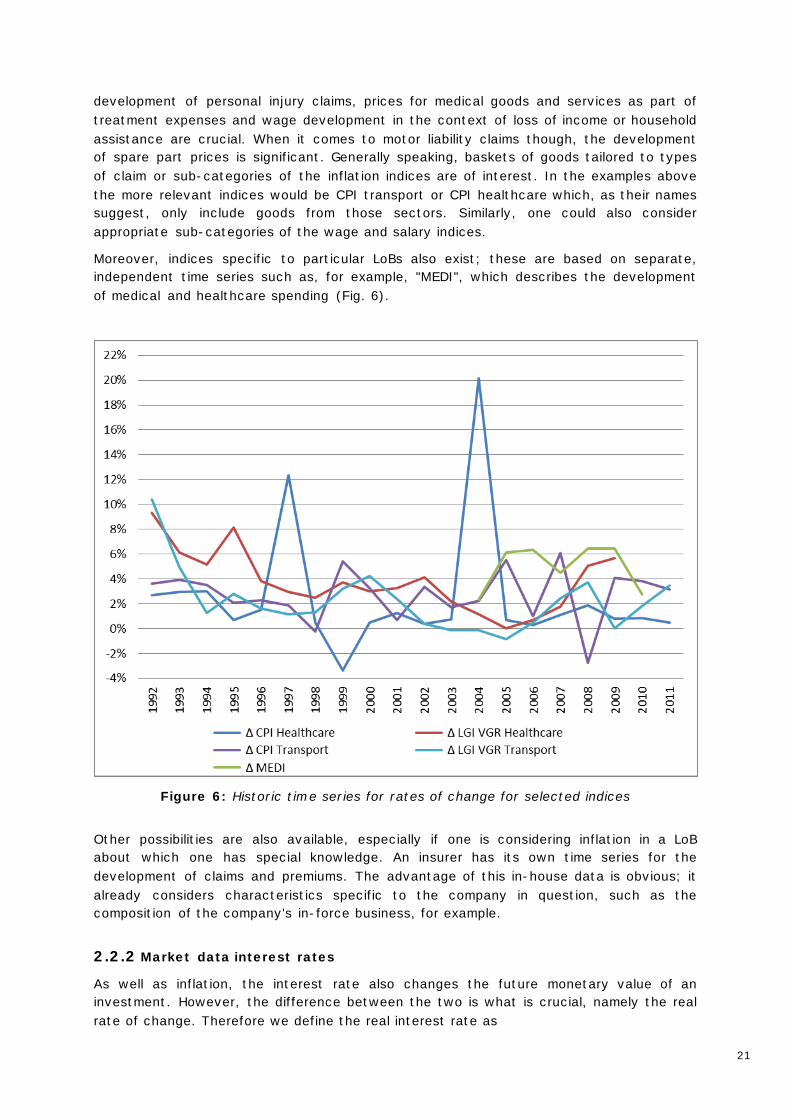
development of personal injury claims, prices for medical goods and services as part of treatment expenses and wage development in the context of loss of income or household assistance are crucial. When it comes to motor liability claims though, the development of spare part prices is significant. Generally speaking, baskets of goods tailored to types of claim or sub-categories of the inflation indices are of interest. In the examples above the more relevant indices would be CPI transport or CPI healthcare which, as their names suggest, only include goods from those sectors. Similarly, one could also consider appropriate sub-categories of the wage and salary indices.
Moreover, indices specific to particular LoBs also exist; these are based on separate, independent time series such as, for example, "MEDI", which describes the development of medical and healthcare spending (Fig. 6).
Figure 6: Historic time series for rates of change for selected indices
Other possibilities are also available, especially if one is considering inflation in a LoB about which one has special knowledge. An insurer has its own time series for the development of claims and premiums. The advantage of this in-house data is obvious; it already considers characteristics specific to the company in question, such as the composition of the company's in-force business, for example.
2.2.2 Market data interest rates
As well as inflation, the interest rate also changes the future monetary value of an investment. However, the difference between the two is what is crucial, namely the real rate of change. Therefore we define the real interest rate as
22
(interest rate)real (interest rate)nominal inflation rate .
In Section 2.1.1 we already anticipated this when we measured inflation using the long-term interest rate, thus indirectly determining the pace of inflation by means of the real interest rate.
2.2.2.1 Money markets
Short-term accounts receivable and securities are traded on the money markets. In this very general definition the money markets represent the counterpart to the capital markets, on which long-term financial transactions are entered into. In international and national statistics, it is common to calculate money market maturities of up to (and including) one year.
The players in the market for central bank money, usually defined as the money market in the narrower sense, are primarily the commercial banks, who use the market to offset micro-economic liquidity surpluses or deficits amongst themselves. The interest rates published by the German Bundesbank refer to the interbank money market.
2.2.2.2 Current yields
Unlike nominal interest rates bond yields represent the actual annual return.
Arranged in types of security:
• fixed-interest securities as a whole
• (covered) bank bonds
• mortgage Pfandbriefe
• public sector Pfandbriefe
• public authority bonds
• listed federal government securities
2.2.2.3 Yield curve on the bond market
The yield curve on the bond market shows the relation between interest rates and maturities of zero-coupon bonds with no default risk. This yield curve data published here are estimates determined on the basis of current yields of coupon bonds.
2.2.2.4 Discount rates as set out in § 253 para. 2 of the German Commercial Code (HGB)
On 29 May 2009, the German Act to Modernise Accounting Law (BilMoG) entered into force. Among other things this law states that reserves with a time to maturity of more than one year have to be discounted with the average market interest rate of the previous seven financial years appropriate for the remaining time to maturity. The Bundesbank determines these discount rates and publishes them every month.
23
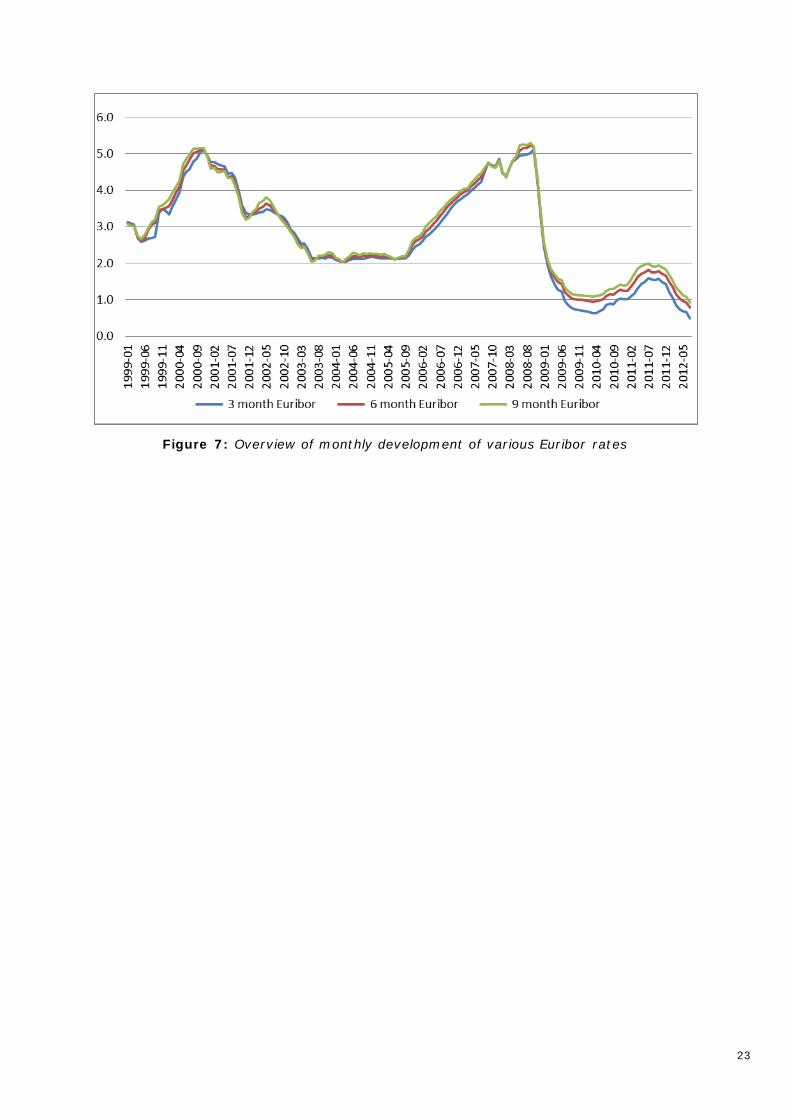
Figure 7: Overview of monthly development of various Euribor rates
24
3 Retrospective look at interest rates and inflation
3.1 Overview of the historic development of interest rates and the CPI
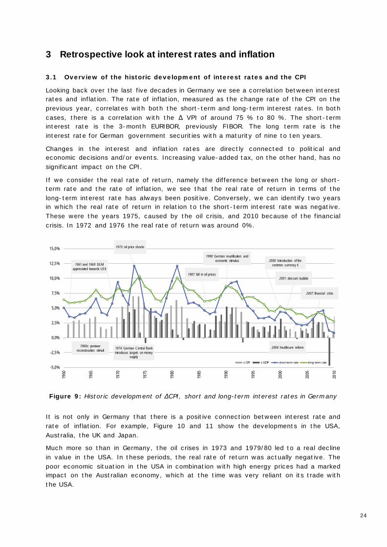
Looking back over the last five decades in Germany we see a correlation between interest rates and inflation. The rate of inflation, measured as the change rate of the CPI on the previous year, correlates with both the short-term and long-term interest rates. In both cases, there is a correlation with the ∆ VPI of around 75 % to 80 %. The short-term interest rate is the 3-month EURIBOR, previously FIBOR. The long term rate is the interest rate for German government securities with a maturity of nine to ten years.
Changes in the interest and inflation rates are directly connected to political and economic decisions and/or events. Increasing value-added tax, on the other hand, has no significant impact on the CPI.
If we consider the real rate of return, namely the difference between the long or short-term rate and the rate of inflation, we see that the real rate of return in terms of the long-term interest rate has always been positive. Conversely, we can identify two years in which the real rate of return in relation to the short-term interest rate was negative. These were the years 1975, caused by the oil crisis, and 2010 because of the financial crisis. In 1972 and 1976 the real rate of return was around 0%.
-5,0%
-2,5%
0,0%
2,5%
5,0%
7,5%
10,0%
12,5%
15,0%
1960
1965
1970
1975
1980
1985
1990
1995
2000
2005
2010
∆ CPI ∆ GDP short-term rate long-term rate
2004: healthcare reform
1990: German reunification und economic stimulus 2000: Introduction of the
common currency €
2001: dot-com bubble
2007: financial crisis
1987: fall in oil prices
1974: German Central Bank introduces targets on money
supply
1973: oil price shocks
1961 and 1969: DEM appreciated towards US$
1960s: postwar reconstruction stimuli
Figure 9: Historic development of ∆CPI, short and long-term interest rates in Germany
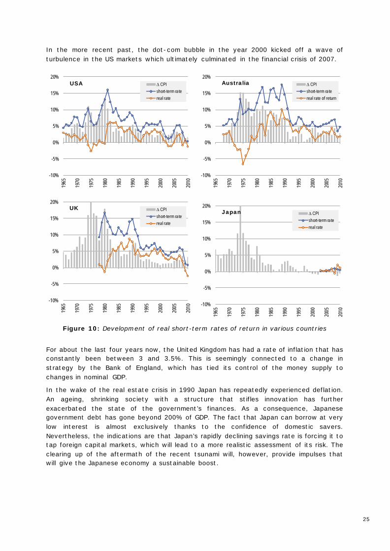
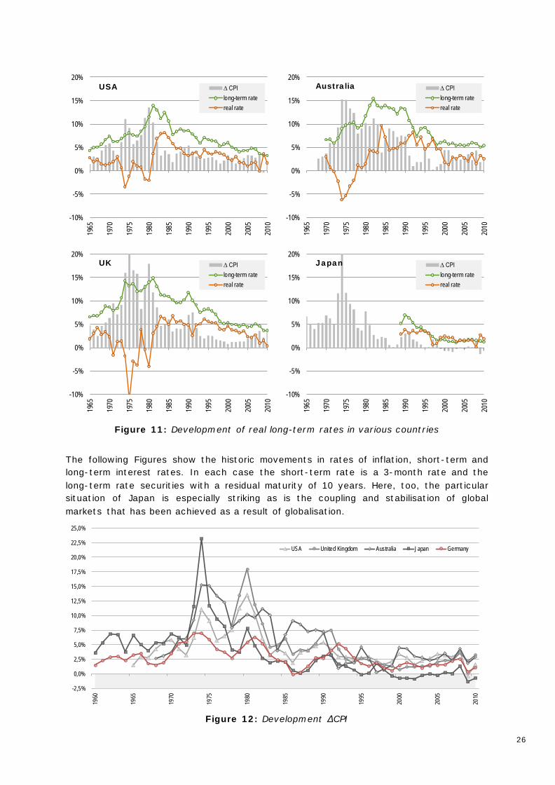
It is not only in Germany that there is a positive connection between interest rate and rate of inflation. For example, Figure 10 and 11 show the developments in the USA, Australia, the UK and Japan.
Much more so than in Germany, the oil crises in 1973 and 1979/80 led to a real decline in value in the USA. In these periods, the real rate of return was actually negative. The poor economic situation in the USA in combination with high energy prices had a marked impact on the Australian economy, which at the time was very reliant on its trade with the USA.
25
In the more recent past, the dot-com bubble in the year 2000 kicked off a wave of turbulence in the US markets which ultimately culminated in the financial crisis of 2007.
-10%
-5%
0%
5%
10%
15%
20%
1965
1970
1975
1980
1985
1990
1995
2000
2005
2010
∆ CPIshort-term ratereal rate
USA
-10%
-5%
0%
5%
10%
15%
20%
1965
1970
1975
1980
1985
1990
1995
2000
2005
2010
∆ CPIshort-term ratereal rate of return
Australia
-10%
-5%
0%
5%
10%
15%
20%
1965
1970
1975
1980
1985
1990
1995
2000
2005
2010
∆ CPIshort-term ratereal rate
UK
-10%
-5%
0%
5%
10%
15%
20%19
65
1970
1975
1980
1985
1990
1995
2000
2005
2010
∆ CPIshort-term ratereal rate
Japan
Figure 10: Development of real short-term rates of return in various countries
For about the last four years now, the United Kingdom has had a rate of inflation that has constantly been between 3 and 3.5%. This is seemingly connected to a change in strategy by the Bank of England, which has tied its control of the money supply to changes in nominal GDP.
In the wake of the real estate crisis in 1990 Japan has repeatedly experienced deflation. An ageing, shrinking society with a structure that stifles innovation has further exacerbated the state of the government’s finances. As a consequence, Japanese government debt has gone beyond 200% of GDP. The fact that Japan can borrow at very low interest is almost exclusively thanks to the confidence of domestic savers. Nevertheless, the indications are that Japan’s rapidly declining savings rate is forcing it to tap foreign capital markets, which will lead to a more realistic assessment of its risk. The clearing up of the aftermath of the recent tsunami will, however, provide impulses that will give the Japanese economy a sustainable boost.
26
-10%
-5%
0%
5%
10%
15%
20%19
65
1970
1975
1980
1985
1990
1995
2000
2005
2010
∆ CPIlong-term ratereal rate
USA
-10%
-5%
0%
5%
10%
15%
20%
1965
1970
1975
1980
1985
1990
1995
2000
2005
2010
∆ CPIlong-term ratereal rate
Australia
-10%
-5%
0%
5%
10%
15%
20%
1965
1970
1975
1980
1985
1990
1995
2000
2005
2010
∆ CPIlong-term ratereal rate
UK
-10%
-5%
0%
5%
10%
15%
20%
1965
1970
1975
1980
1985
1990
1995
2000
2005
2010
∆ CPIlong-term ratereal rate
Japan
Figure 11: Development of real long-term rates in various countries
The following Figures show the historic movements in rates of inflation, short-term and long-term interest rates. In each case the short-term rate is a 3-month rate and the long-term rate securities with a residual maturity of 10 years. Here, too, the particular situation of Japan is especially striking as is the coupling and stabilisation of global markets that has been achieved as a result of globalisation.
-2,5%
0,0%
2,5%
5,0%
7,5%
10,0%
12,5%
15,0%
17,5%
20,0%
22,5%
25,0%
1960
1965
1970
1975
1980
1985
1990
1995
2000
2005
2010
USA United Kingdom Australia Japan Germany
Figure 12: Development ∆CPI
27
-2,5%
0,0%
2,5%
5,0%
7,5%
10,0%
12,5%
15,0%
17,5%
20,0%
22,5%
25,0%
1960
1965
1970
1975
1980
1985
1990
1995
2000
2005
2010
USA United Kingdom Australia Japan Germany
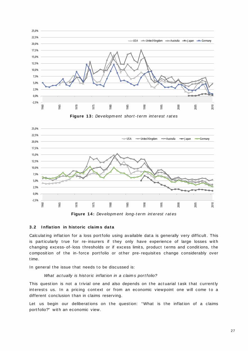
Figure 13: Development short-term interest rates
-2,5%
0,0%
2,5%
5,0%
7,5%
10,0%
12,5%
15,0%
17,5%
20,0%
22,5%
25,0%
1960
1965
1970
1975
1980
1985
1990
1995
2000
2005
2010
USA United Kingdom Australia Japan Germany
Figure 14: Development long-term interest rates
3.2 Inflation in historic claims data
Calculating inflation for a loss portfolio using available data is generally very difficult. This is particularly true for re-insurers if they only have experience of large losses with changing excess-of-loss thresholds or if excess limits, product terms and conditions, the composition of the in-force portfolio or other pre-requisites change considerably over time.
In general the issue that needs to be discussed is:
What actually is historic inflation in a claims portfolio?
This question is not a trivial one and also depends on the actuarial task that currently interests us. In a pricing context or from an economic viewpoint one will come to a different conclusion than in claims reserving.
Let us begin our deliberations on the question: “What is the inflation of a claims portfolio?” with an economic view.

28
In economic terms, inflation means the change in the average price of a given basket of goods. Transferred to a claims portfolio this would mean considering a “basket of goods” consisting of claims. These claims would be fixed by characteristics such as,
• Personal injury / Property claims • Run-off period • Type of injury • Degree of injury • Damaged parts of a motor vehicle.
The characteristics would be selected to provide a “representative” cross-section of the claims portfolio. The individual claims would be weighted so as to suit the composition of the claims portfolio.
Using this “model claims portfolio” one would then henceforth try to observe average price increases and use them to define “claims inflation”.
Determining the claims inflation we have just described is not trivial (GLM, weighting process) and is complicated. In practice, it will usually be difficult to implement, if indeed, it is possible at all, owing to a lack of data availability.
Moreover, if we consider claims reserving, the question arises: Is this “economic claims inflation” view what we actually need in claims reserving?
In reserving we usually have a different view of inflation. In reserving, inflation is a “diagonal effect” in the payment triangles, which affects claims data and run-off factors along the diagonals and which may cause so much distortion that reserves are over- or under-estimated. This effect differs from the economic inflation described above since the diagonals of the run-off triangles are influenced by a multitude of effects such as:
• Changes in claims handling • Technical and medical innovations • Legal changes • Changes in the composition of the claims portfolio • Composition of the customer portfolio • Products and range of benefits and services • Trends for claims frequency and claims levels
Which of these effects should be subsumed under inflationary aspects is often not quite clear and depends on one’s point of view. For a re-insurer, claims frequency may well count as inflation – if one considers XL treaties – though not necessarily for a primary insurer.
For those effects that should not be subsumed under inflation one should consider whether adjustment is possible though, in practice, this is unfortunately often difficult to do.
In the following we shall focus on the view of inflation in claims reserving. That means we will view inflation as a “diagonal effect” that has to be determined. In so doing, we will present two methods that will help to provide an approximate impression of the inflation contained in run-off triangles. These are “determining inflation from an accident year view” and the separation method, which is well known from the relevant literature. These two methods will be presented and applied to real data. Our results will then be discussed.
29
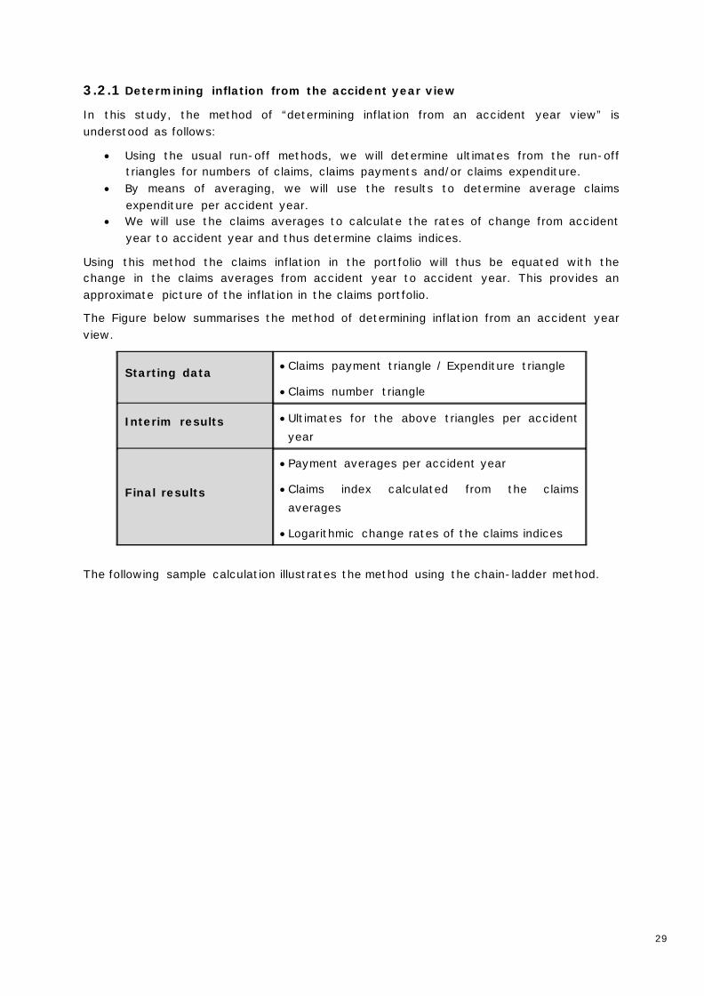
3.2.1 Determining inflation from the accident year view
In this study, the method of “determining inflation from an accident year view” is understood as follows:
• Using the usual run-off methods, we will determine ultimates from the run-off triangles for numbers of claims, claims payments and/or claims expenditure.
• By means of averaging, we will use the results to determine average claims expenditure per accident year.
• We will use the claims averages to calculate the rates of change from accident year to accident year and thus determine claims indices.
Using this method the claims inflation in the portfolio will thus be equated with the change in the claims averages from accident year to accident year. This provides an approximate picture of the inflation in the claims portfolio.
The Figure below summarises the method of determining inflation from an accident year view.
Starting data • Claims payment triangle / Expenditure triangle
• Claims number triangle
Interim results • Ultimates for the above triangles per accident year
Final results
• Payment averages per accident year
• Claims index calculated from the claims averages
• Logarithmic change rates of the claims indices
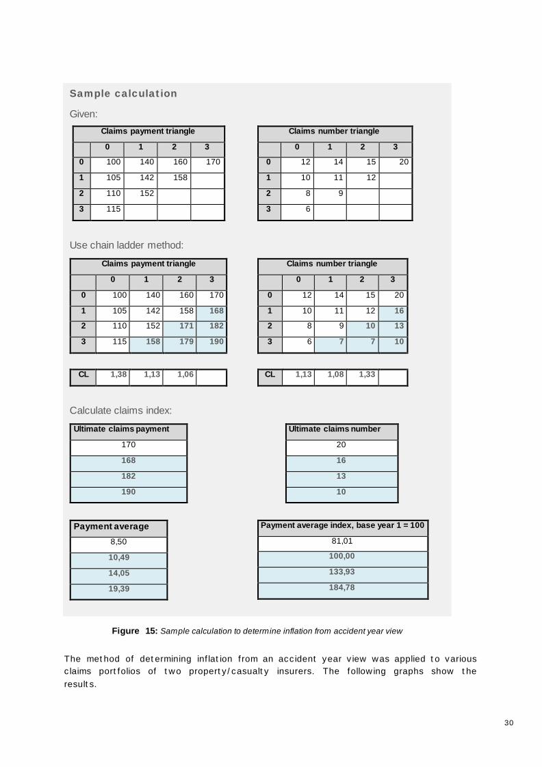
The following sample calculation illustrates the method using the chain-ladder method.
30
Ergebnisse
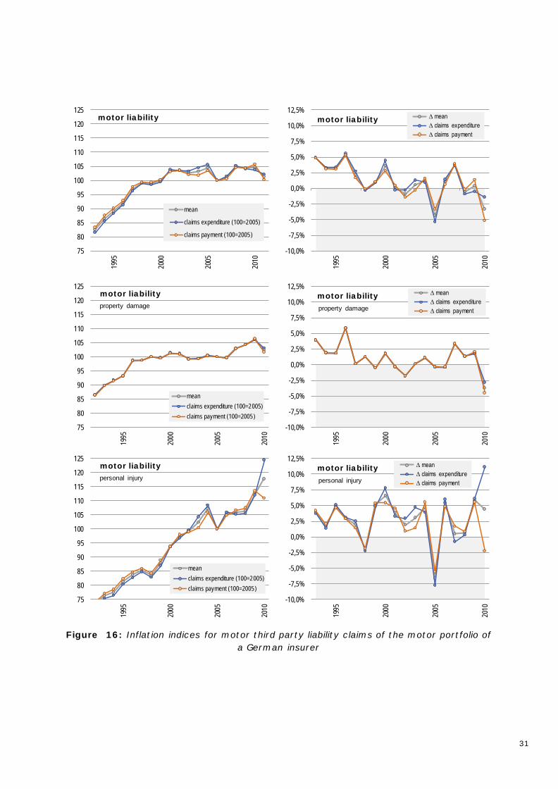
The method of determining inflation from an accident year view was applied to various claims portfolios of two property/casualty insurers. The following graphs show the results.
Sample calculation
Given: Claims payment triangle
0 1 2 3
0 100 140 160 170
1 105 142 158
2 110 152
3 115
Claims number triangle
0 1 2 3
0 12 14 15 20
1 10 11 12
2 8 9
3 6
Use chain ladder method:
Claims payment triangle
0 1 2 3
0 100 140 160 170
1 105 142 158 168
2 110 152 171 182
3 115 158 179 190
CL 1,38 1,13 1,06
Claims number triangle
0 1 2 3
0 12 14 15 20
1 10 11 12 16
2 8 9 10 13
3 6 7 7 10
CL 1,13 1,08 1,33
Calculate claims index:
Ultimate claims payment
170
168
182
190
Ultimate claims number
20
16
13
10
Payment average
8,50
10,49
14,05
19,39
Payment average index, base year 1 = 100
81,01
100,00
133,93
184,78
Figure 15: Sample calculation to determine inflation from accident year view
Sample calculation
Given: Claims payment triangle
0 1 2 3
0 100 140 160 170
1 105 142 158
2 110 152
3 115
Claims number triangle
0 1 2 3
0 12 14 15 20
1 10 11 12
2 8 9
3 6
Use chain ladder method:
Claims payment triangle
0 1 2 3
0 100 140 160 170
1 105 142 158 168
2 110 152 171 182
3 115 158 179 190
CL 1,38 1,13 1,06
Claims number triangle
0 1 2 3
0 12 14 15 20
1 10 11 12 16
2 8 9 10 13
3 6 7 7 10
CL 1,13 1,08 1,33
Calculate claims index:
Ultimate claims payment
170
168
182
190
Ultimate claims number
20
16
13
10
Payment average 8,50
10,49
14,05
19,39
Payment average index, base year 1 = 100
81,01
100,00
133,93
184,78
31
75
80
85
90
95
100
105
110
115
120
12519
95
2000
2005
2010
mean
claims expenditure (100=2005)
claims payment (100=2005)
motor liability
-10,0%
-7,5%
-5,0%
-2,5%
0,0%
2,5%
5,0%
7,5%
10,0%
12,5%
1995
2000
2005
2010
∆ mean∆ claims expenditure∆ claims payment
motor liability
75
80
85
90
95
100
105
110
115
120
125
1995
2000
2005
2010
meanclaims expenditure (100=2005)claims payment (100=2005)
motor liabilityproperty damage
-10,0%
-7,5%
-5,0%
-2,5%
0,0%
2,5%
5,0%
7,5%
10,0%
12,5%
1995
2000
2005
2010
∆ mean∆ claims expenditure∆ claims payment
motor liabilityproperty damage
75
80
85
90
95
100
105
110
115
120
125
1995
2000
2005
2010
meanclaims expenditure (100=2005)claims payment (100=2005)
motor liabilitypersonal injury
-10,0%
-7,5%
-5,0%
-2,5%
0,0%
2,5%
5,0%
7,5%
10,0%
12,5%
1995
2000
2005
2010
∆ mean∆ claims expenditure∆ claims payment
motor liabilitypersonal injury
Figure 16: Inflation indices for motor third party liability claims of the motor portfolio of a German insurer
32
70
75
80
85
90
95
100
105
110
1995
2000
2005
2010
Insurer 1
Insurer 2
motor liability
-10,0%
-7,5%
-5,0%
-2,5%
0,0%
2,5%
5,0%
7,5%
10,0%
12,5%
1995
2000
2005
2010
Insurer 1Insurer 2
motor liability
25
50
75
100
125
1995
2000
2005
2010
motor liabilitythird patry liabilityarchitcts liabilitymedic care
-50,0%
-30,0%
-10,0%
10,0%
30,0%
50,0%
1995
2000
2005
2010
motor liabilitythird party liabilityarchitects liabilitymedic care
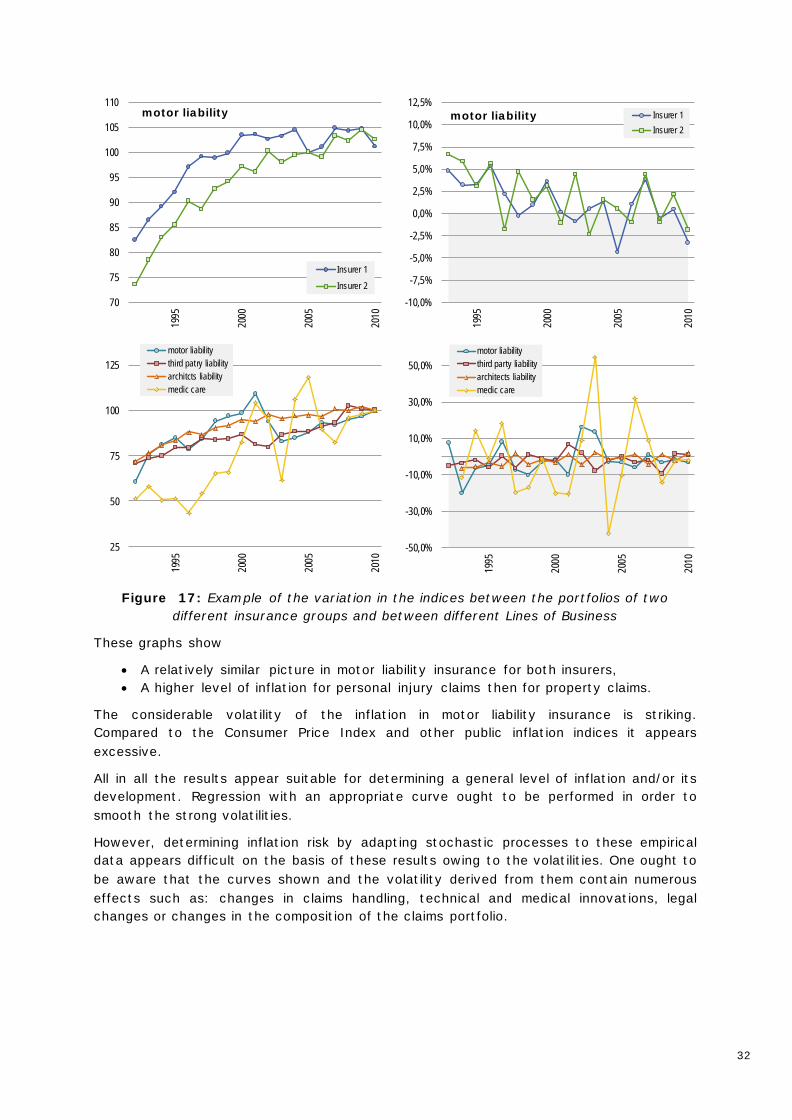
Figure 17: Example of the variation in the indices between the portfolios of two different insurance groups and between different Lines of Business
These graphs show
• A relatively similar picture in motor liability insurance for both insurers, • A higher level of inflation for personal injury claims then for property claims.
The considerable volatility of the inflation in motor liability insurance is striking. Compared to the Consumer Price Index and other public inflation indices it appears excessive.
All in all the results appear suitable for determining a general level of inflation and/or its development. Regression with an appropriate curve ought to be performed in order to smooth the strong volatilities.
However, determining inflation risk by adapting stochastic processes to these empirical data appears difficult on the basis of these results owing to the volatilities. One ought to be aware that the curves shown and the volatility derived from them contain numerous effects such as: changes in claims handling, technical and medical innovations, legal changes or changes in the composition of the claims portfolio.
33
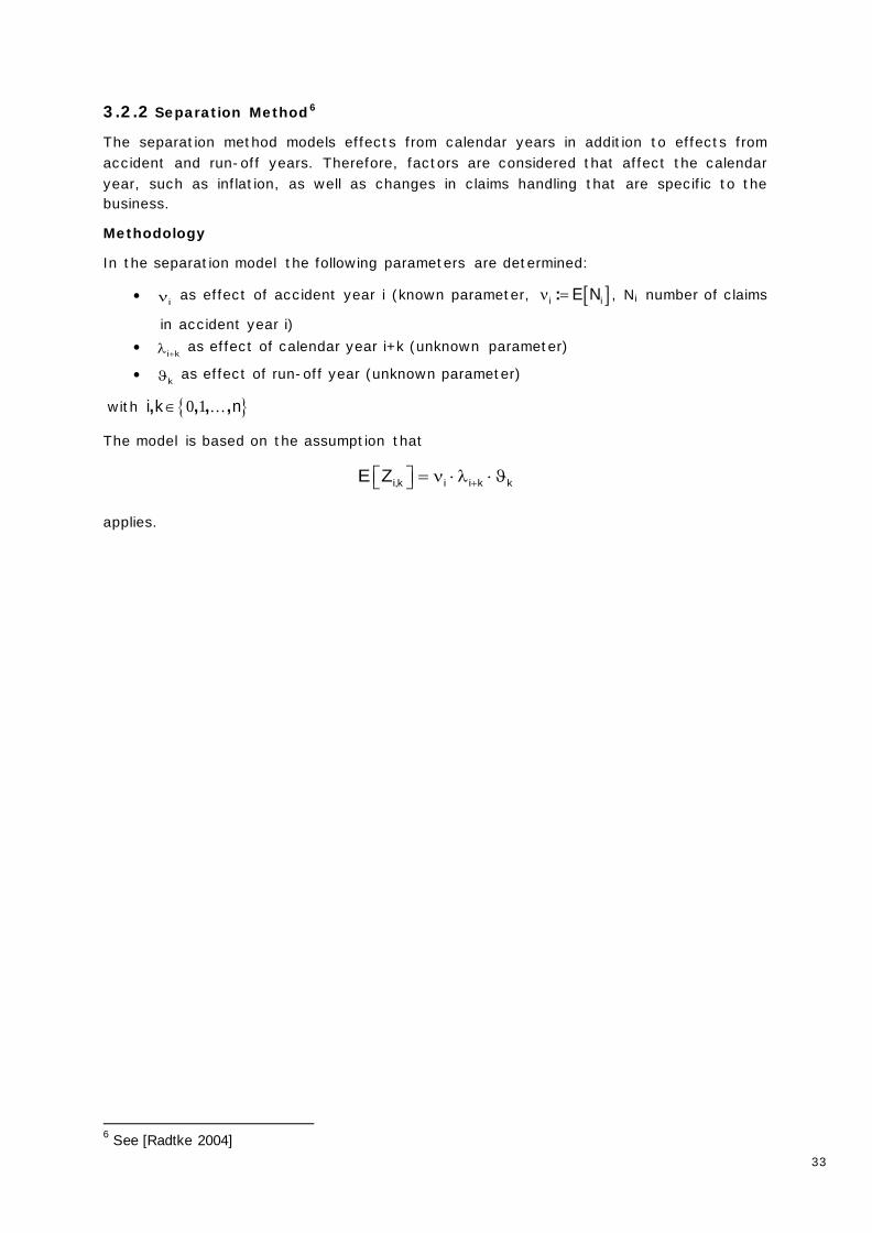
3.2.2 Separation Method6
The separation method models effects from calendar years in addition to effects from accident and run-off years. Therefore, factors are considered that affect the calendar year, such as inflation, as well as changes in claims handling that are specific to the business.
Methodology
In the separation model the following parameters are determined:
• iν as effect of accident year i (known parameter, [ ]i iE Nν =: , Ni number of claims
in accident year i) • i k+λ as effect of calendar year i+k (unknown parameter)
• kϑ as effect of run-off year (unknown parameter)
with { }0 1i k n∈ , , , ,
The model is based on the assumption that
i,k i i k kE Z + = ν ⋅ λ ⋅ ϑ
applies.
6 See [Radtke 2004]
34
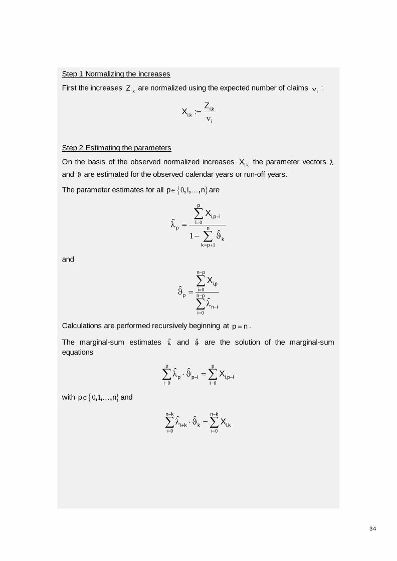
Step 1 Normalizing the increases
First the increases i,kZ are normalized using the expected number of claims iν :
i,ki,k
i
ZX :=
ν
Step 2 Estimating the parameters
On the basis of the observed normalized increases i,kX the parameter vectors λ
and ϑ are estimated for the observed calendar years or run-off years.
The parameter estimates for all { }0 1p n∈ , , , are
0
11
p
i,p ii
p n
kk p
Xˆ
ˆ
−=
= +
λ =− ϑ
∑
∑
and
0
0
n p
i,pi
p n p
n ii
Xˆ
ˆ
−
=−
−=
ϑ =λ
∑
∑
Calculations are performed recursively beginning at p n= .
The marginal-sum estimates λ̂ and ϑ̂ are the solution of the marginal-sum equations
0 0
p p
p p i i,p ii i
ˆ ˆ X− −= =
λ ⋅ ϑ =∑ ∑
with { }0 1p n∈ , , , and
0 0
n k n k
i k k i,ki i
ˆ ˆ X− −
+= =
λ ⋅ ϑ =∑ ∑
35
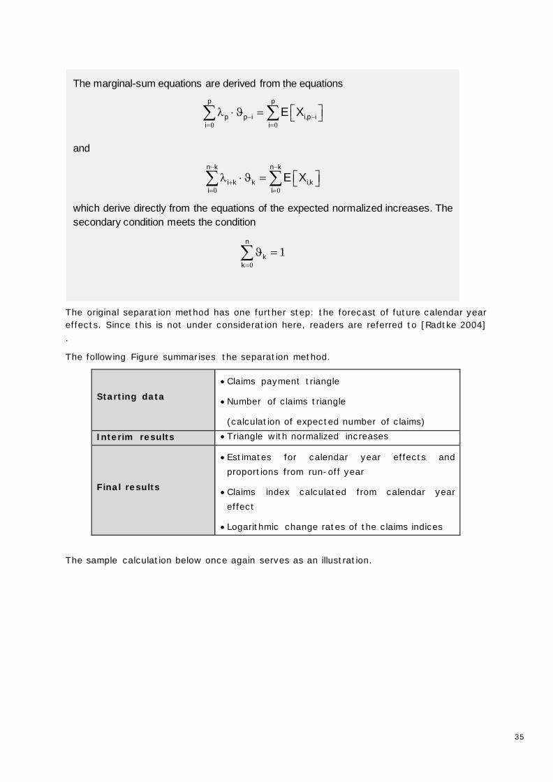
The marginal-sum equations are derived from the equations
0 0
p p
p p i i,p ii i
E X− −= =
λ ⋅ ϑ = ∑ ∑
and
0 0
n k n k
i k k i,ki i
E X− −
+= =
λ ⋅ ϑ = ∑ ∑
which derive directly from the equations of the expected normalized increases. The secondary condition meets the condition
01
n
kk=
ϑ =∑
The original separation method has one further step: the forecast of future calendar year effects. Since this is not under consideration here, readers are referred to [Radtke 2004] .
The following Figure summarises the separation method.
Starting data • Claims payment triangle
• Number of claims triangle
(calculation of expected number of claims) Interim results • Triangle with normalized increases
Final results
• Estimates for calendar year effects and proportions from run-off year
• Claims index calculated from calendar year effect
• Logarithmic change rates of the claims indices
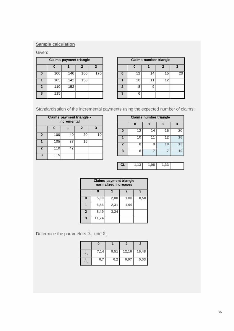
The sample calculation below once again serves as an illustration.
36
Sample calculation
Given: Claims payment triangle
0 1 2 3
0 100 140 160 170
1 105 142 158
2 110 152
3 115
Claims number triangle
0 1 2 3
0 12 14 15 20
1 10 11 12
2 8 9
3 6
Standardisation of the incremental payments using the expected number of claims:
Claims payment triangle - incremental
0 1 2 3
0 100 40 20 10
1 105 37 16
2 110 42
3 115
Claims number triangle
0 1 2 3
0 12 14 15 20
1 10 11 12 16
2 8 9 10 13
3 6 7 7 10
CL 1,13 1,08 1,33
Claims payment triangle normalized increases
0 1 2 3
0 5,00 2,00 1,00 0,50
1 6,56 2,31 1,00
2 8,49 3,24
3 11,74
Determine the parameters p pˆ ˆ und λ ϑ
0 1 2 3
pλ̂ 7,14 9,51 12,16 16,48
pϑ̂ 0,7 0,2 0,07 0,03
37
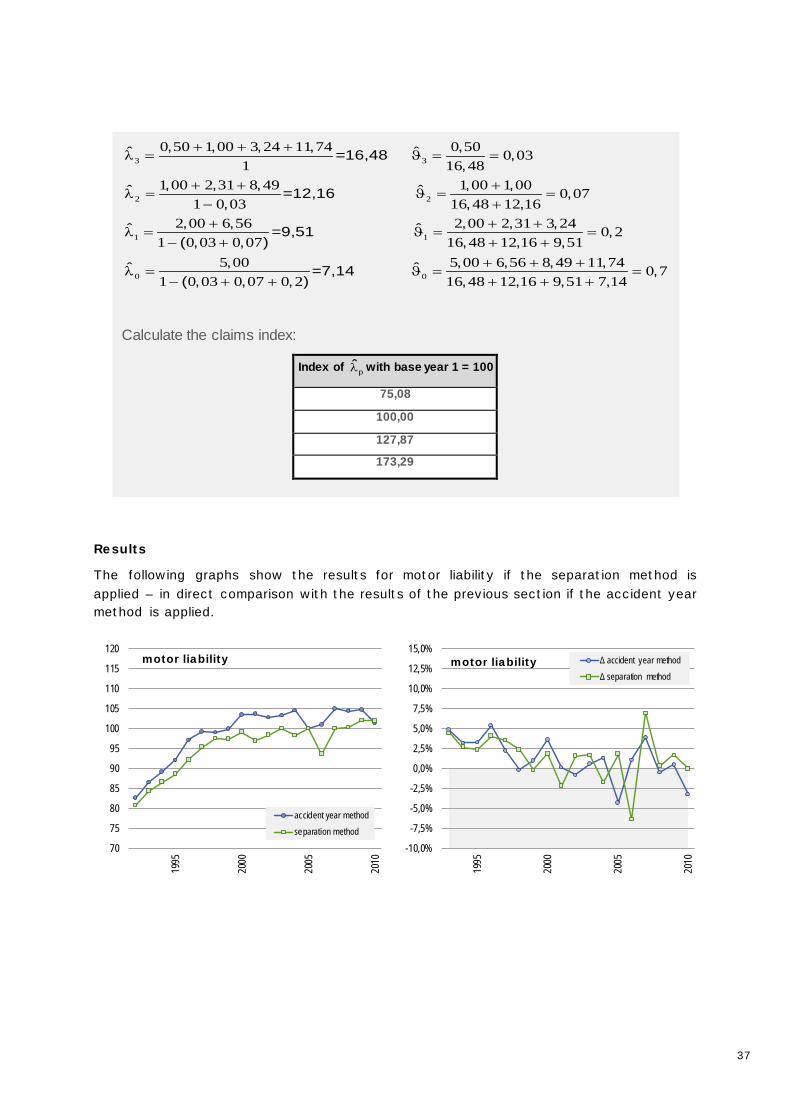
Results
The following graphs show the results for motor liability if the separation method is applied – in direct comparison with the results of the previous section if the accident year method is applied.
70
75
80
85
90
95
100
105
110
115
120
1995
2000
2005
2010
accident year method
separation method
motor liability
-10,0%
-7,5%
-5,0%
-2,5%
0,0%
2,5%
5,0%
7,5%
10,0%
12,5%
15,0%
1995
2000
2005
2010
Δ accident year method
Δ separation methodmotor liability
3 3
2 2
1 1
0 50 1 00 3 24 11 74 0 50 0 031 16 48
1 00 2 31 8 49 1 00 1 00 0 071 0 03 16 48 12 16
2 00 6 56 2 00 2 31 3 241 0 03 0 07
, , , , ,ˆ ˆ=16,48 ,,
, , , , ,ˆ ˆ=12,16 ,, , ,
, , , , ,ˆ ˆ=9,51 ( , , )
+ + +λ = ϑ = =
+ + +λ = ϑ = =
− ++ + +
λ = ϑ =− +
0 0
0 216 48 12 16 9 51
5 00 5 00 6 56 8 49 11 74 0 71 0 03 0 07 0 2 16 48 12 16 9 51 7 14
,, , ,
, , , , ,ˆ ˆ=7,14 ,( , , , ) , , , ,
=+ ++ + +
λ = ϑ = =− + + + + +
Calculate the claims index:
Index of pλ̂ with base year 1 = 100
75,08
100,00
127,87
173,29

38
70
75
80
85
90
95
100
105
110
115
120
1995
2000
2005
2010
accident year method
separation method
motor liability
property damage
-10,0%
-7,5%
-5,0%
-2,5%
0,0%
2,5%
5,0%
7,5%
10,0%
12,5%
1995
2000
2005
2010
Δ accident year method
Δ separation methodmotor liabilityproperty damage
70
75
80
85
90
95
100
105
110
115
120
1995
2000
2005
2010
accident year method
separation method
motor liabilitypersonal injury
-10,0%
-7,5%
-5,0%
-2,5%
0,0%
2,5%
5,0%
7,5%
10,0%
12,5%
15,0%
1995
2000
2005
2010
Δ accident year method
Δ separation methodmotor liabilitypersonal injury
Figure 18: Comparison of accident year method and separation method
Essentially we can state that both methods produced qualitatively similar results in terms of level of inflation and volatility. This was echoed in calculations for other lines of lusiness and companies that were performed as part of this research but are not published here.
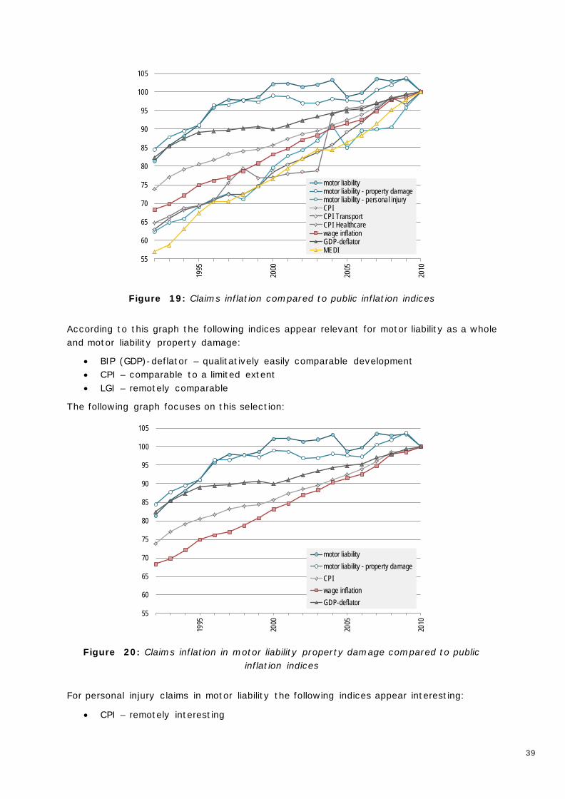
3.2.3 Comparing claims portfolio inflation with public inflation indices
If it is not possible to calculate inflation using the data one usually has no other choice but to make assumptions about the inflation contained in the data and to construct a claims index on the basis of a presumably “suitable” inflation index (e.g., wages and earnings, Consumer Price Index or also combinations of similar indices of this type). Frequently, assumptions about superimposed inflation are made, for example, to cover price increases in health and medical care.
Below, as an example, we compare inflation determined using the accident year method with that contained in a selection of publicly available indices for motor liability. We distinguish between motor liability as a whole as well as property damage and personal injury in motor liability.
39
55
60
65
70
75
80
85
90
95
100
105
1995
2000
2005
2010
motor liabilitymotor liability - property damagemotor liability - personal injuryCPICPI TransportCPI Healthcarewage inflationGDP-deflatorMEDI
Figure 19: Claims inflation compared to public inflation indices
According to this graph the following indices appear relevant for motor liability as a whole and motor liability property damage:
• BIP (GDP)-deflator – qualitatively easily comparable development • CPI – comparable to a limited extent • LGI – remotely comparable
The following graph focuses on this selection:
55
60
65
70
75
80
85
90
95
100
105
1995
2000
2005
2010
motor liabilitymotor liability - property damageCPIwage inflationGDP-deflator
Figure 20: Claims inflation in motor liability property damage compared to public inflation indices
For personal injury claims in motor liability the following indices appear interesting:
• CPI – remotely interesting
40
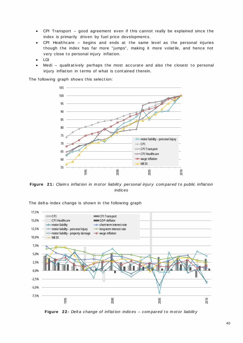
• CPI Transport – good agreement even if this cannot really be explained since the index is primarily driven by fuel price developments.
• CPI Healthcare – begins and ends at the same level as the personal injuries though the index has far more “jumps”, making it more volatile, and hence not very close to personal injury inflation.
• LGI • Medi – qualitatively perhaps the most accurate and also the closest to personal
injury inflation in terms of what is contained therein.
The following graph shows this selection:
55
60
65
70
75
80
85
90
95
100
10519
95
2000
2005
2010
motor liability - personal injuryCPICPI TransportCPI Healthcarewage inflationMEDI
Figure 21: Claims inflation in motor liability personal injury compared to public inflation indices
The delta-index change is shown in the following graph
-7,5%
-5,0%
-2,5%
0,0%
2,5%
5,0%
7,5%
10,0%
12,5%
15,0%
17,5%
1995
2000
2005
2010
CPI CPI TransportCPI Healthcare GDP-deflatormotor liability short-term interest ratemotor liability - personal injury long-term interest ratemotor liability - property damage wage inflationMEDI
Figure 22: Delta change of inflation indices – compared to motor liability
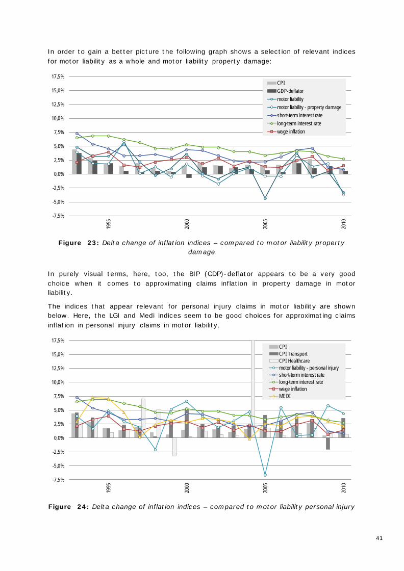
41
In order to gain a better picture the following graph shows a selection of relevant indices for motor liability as a whole and motor liability property damage:
-7,5%
-5,0%
-2,5%
0,0%
2,5%
5,0%
7,5%
10,0%
12,5%
15,0%
17,5%
1995
2000
2005
2010
CPIGDP-deflatormotor liabilitymotor liability - property damageshort-term interest ratelong-term interest ratewage inflation
Figure 23: Delta change of inflation indices – compared to motor liability property damage
In purely visual terms, here, too, the BIP (GDP)-deflator appears to be a very good choice when it comes to approximating claims inflation in property damage in motor liability.
The indices that appear relevant for personal injury claims in motor liability are shown below. Here, the LGI and Medi indices seem to be good choices for approximating claims inflation in personal injury claims in motor liability.
-7,5%
-5,0%
-2,5%
0,0%
2,5%
5,0%
7,5%
10,0%
12,5%
15,0%
17,5%
1995
2000
2005
2010
CPICPI TransportCPI Healthcaremotor liability - personal injuryshort-term interest ratelong-term interest ratewage inflationMEDI
Figure 24: Delta change of inflation indices – compared to motor liability personal injury
42
3.3 Including inflation assumptions in the calculation of reserves
Calculating reserves in property/casualty insurance is usually done on the basis of run-off triangles with historic data. These data usually implicitly include the effect of past inflation. If actuaries wish to calculate reserves they are faced with the question:
• Should the run-off triangle remain unchanged? If so the run off procedures are simply applied to the historic data; the inflation that is implicitly present in the triangle will thus also be continued into the future.
• Or should the run-off triangle be adjusted for inflation? If so, one requires knowledge of the past inflation inherent in the triangle. This enables the triangle to be adjusted for inflation. Run-off procedures can then be applied to this triangle. Finally assumptions about future inflation have to be made in order to be able to consider future inflation in the projected cash flow.
The literature on actuarial reserving often states that “inflation has to be considered” or “triangles should be adjusted for inflation if appropriate”. But what does this actually mean in practice? How can this adjustment be done? And what lever does inflation have on the level of reserves when it comes to calculating them?
These issues are addressed below. It becomes evident that, in practice, “adjusting for inflation” throws up considerable problems.
3.3.1 Calculating reserves adjusted for inflation – Method
When calculating the best estimate reserve that is adjusted for inflation two key assumptions concerning the inflation have to be made:
(1.) Assumption of a time line for the historic inflation contained in the triangles, e.g., an inflation time line for the years from 1975 to the present.
(2.) Assumption of a time line for future inflation that will have an impact on the projected cash flow of the claims portfolio – e.g., an inflation time line from the present until 2075.
On the basis of these two assumptions the calculation of the reserves based on a payment triangle can then be done as follows:
• The payment triangle is represented incrementally. • Using time line (1) for historic inflation the incremental payments – i.e., the entire
cash flow of the run-off triangle – can be converted to the present cash value. This produces a run-off triangle, adjusted for the inflation assumption, which (perhaps?) better meets the conditions of chain-ladder or other models.
• The reserving methods (e.g., chain ladder, …) can then be calculated on the adjusted triangle; this produces a future cash flow projection, i.e., the bottom triangle of the rectangle is filled. All these fields are still calculated in the present cash value.
• In one further step the projection has to be further transformed using the assumed future rates of inflation – i.e., time line (2) – so that the projected future cash flow can be updated to the value of the respective future year.
• This then allows the reserve to be calculated as usual: the future cash flows (now containing inflation) – i.e., the fields of the bottom right hand triangle – are simply added up.
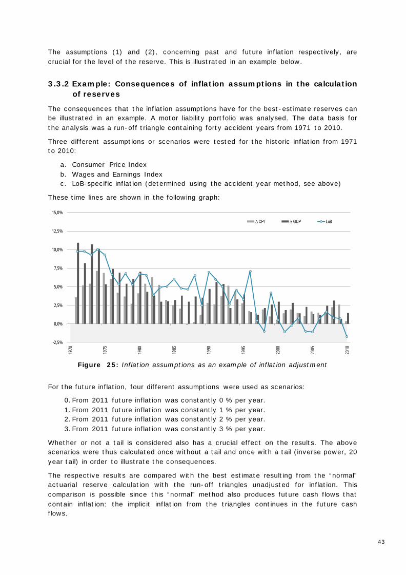
43
The assumptions (1) and (2), concerning past and future inflation respectively, are crucial for the level of the reserve. This is illustrated in an example below.
3.3.2 Example: Consequences of inflation assumptions in the calculation of reserves
The consequences that the inflation assumptions have for the best-estimate reserves can be illustrated in an example. A motor liability portfolio was analysed. The data basis for the analysis was a run-off triangle containing forty accident years from 1971 to 2010.
Three different assumptions or scenarios were tested for the historic inflation from 1971 to 2010:
a. Consumer Price Index b. Wages and Earnings Index c. LoB-specific inflation (determined using the accident year method, see above)
These time lines are shown in the following graph:
-2,5%
0,0%
2,5%
5,0%
7,5%
10,0%
12,5%
15,0%
1970
1975
1980
1985
1990
1995
2000
2005
2010
∆ CPI ∆ GDP LoB
Figure 25: Inflation assumptions as an example of inflation adjustment
For the future inflation, four different assumptions were used as scenarios:
0. From 2011 future inflation was constantly 0 % per year. 1. From 2011 future inflation was constantly 1 % per year. 2. From 2011 future inflation was constantly 2 % per year. 3. From 2011 future inflation was constantly 3 % per year.
Whether or not a tail is considered also has a crucial effect on the results. The above scenarios were thus calculated once without a tail and once with a tail (inverse power, 20 year tail) in order to illustrate the consequences.
The respective results are compared with the best estimate resulting from the “normal” actuarial reserve calculation with the run-off triangles unadjusted for inflation. This comparison is possible since this “normal” method also produces future cash flows that contain inflation: the implicit inflation from the triangles continues in the future cash flows.
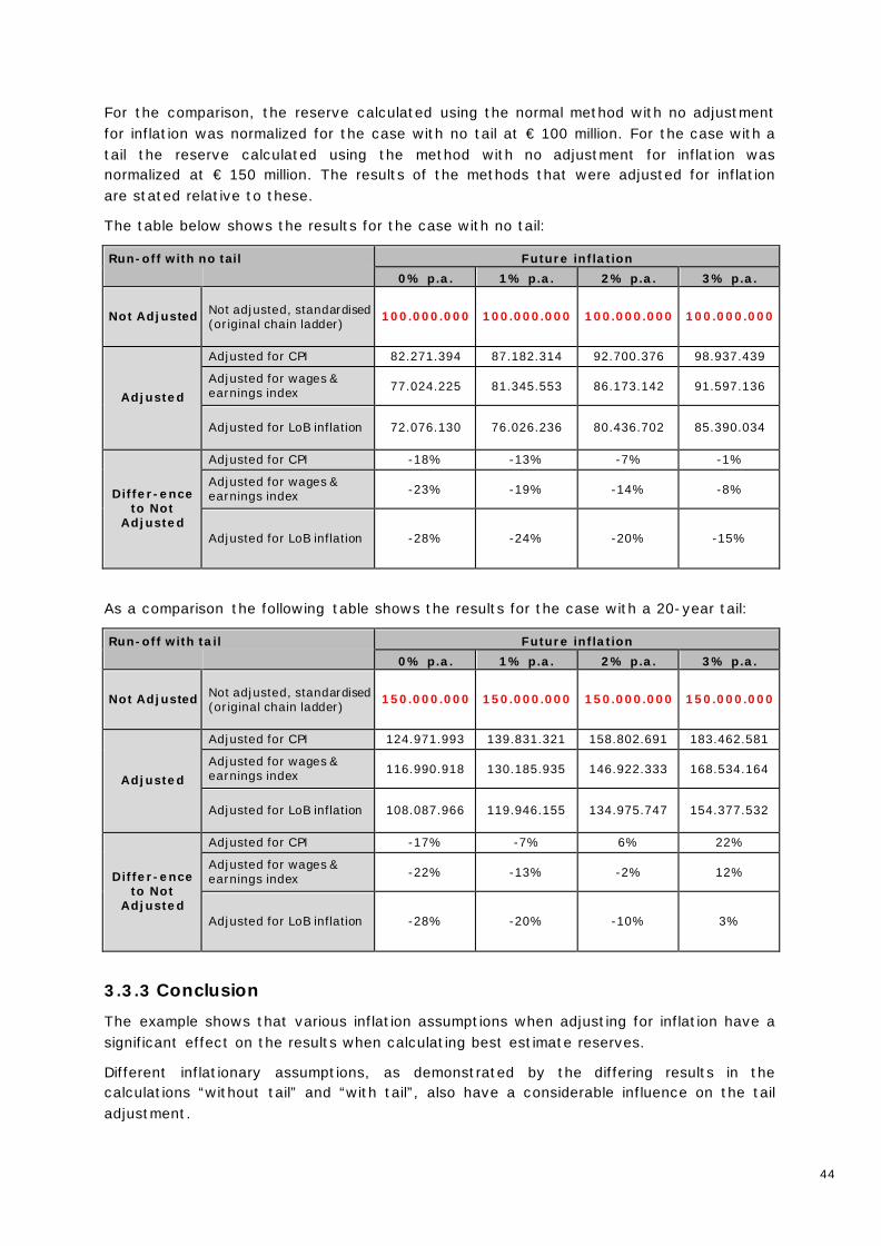
44
For the comparison, the reserve calculated using the normal method with no adjustment for inflation was normalized for the case with no tail at € 100 million. For the case with a tail the reserve calculated using the method with no adjustment for inflation was normalized at € 150 million. The results of the methods that were adjusted for inflation are stated relative to these.
The table below shows the results for the case with no tail:
Run-off with no tail Future inflation 0% p.a. 1% p.a. 2% p.a. 3% p.a.
Not Adjusted Not adjusted, standardised (original chain ladder) 100.000.000 100.000.000 100.000.000 100.000.000
Adjusted
Adjusted for CPI 82.271.394 87.182.314 92.700.376 98.937.439
Adjusted for wages & earnings index 77.024.225 81.345.553 86.173.142 91.597.136
Adjusted for LoB inflation 72.076.130 76.026.236 80.436.702 85.390.034
Differ-ence to Not
Adjusted
Adjusted for CPI -18% -13% -7% -1%
Adjusted for wages & earnings index -23% -19% -14% -8%
Adjusted for LoB inflation -28% -24% -20% -15%
As a comparison the following table shows the results for the case with a 20-year tail:
Run-off with tail Future inflation 0% p.a. 1% p.a. 2% p.a. 3% p.a.
Not Adjusted Not adjusted, standardised (original chain ladder) 150.000.000 150.000.000 150.000.000 150.000.000
Adjusted
Adjusted for CPI 124.971.993 139.831.321 158.802.691 183.462.581
Adjusted for wages & earnings index 116.990.918 130.185.935 146.922.333 168.534.164
Adjusted for LoB inflation 108.087.966 119.946.155 134.975.747 154.377.532
Differ-ence to Not
Adjusted
Adjusted for CPI -17% -7% 6% 22%
Adjusted for wages & earnings index -22% -13% -2% 12%
Adjusted for LoB inflation -28% -20% -10% 3%
3.3.3 Conclusion The example shows that various inflation assumptions when adjusting for inflation have a significant effect on the results when calculating best estimate reserves.
Different inflationary assumptions, as demonstrated by the differing results in the calculations “without tail” and “with tail”, also have a considerable influence on the tail adjustment.

45
Adjusting triangles for inflation thus raises more questions than answers. What is the “correct” inflationary assumption? This question is almost impossible to answer. This applies all the more since the results produced by adjusting for LoB-specific inflation are far away from the results produced when calculating with no adjustment. This shows the problems associated with adjusting run-off triangles when calculating reserves.
Hence the following recommendation:
• In normal circumstances, run-off triangles should not be adjusted for inflation. o Changes in the triangles caused by inflation (e.g., effects of the reform of
the RVG - German Lawyer Remuneration Act - in legal expenses insurance) can usually be managed by deleting a diagonal from the run-off factors. A different level of inflation in the past can be “blanked out” by only using current diagonals – e.g., from the last 10 years.
o It is important to consider future inflation and the consequences it will have on future cash flows. The unadjusted triangle ought to be used as usual. Various inflation scenarios can then be applied to the resulting future cash flows. This provides a picture of the effects of future inflation that is both easy to understand and interpret in terms of sensitivity analyses. The inflation scenarios should be developed on the basis of historic inflation – see below for guidance on how to develop such scenarios. One must consider, too, that implicit inflation is already contained in the projected cash flows; thus scenarios may only incorporate inflation that goes beyond this.
• Adjusting run-off triangles for inflation should only be done if one truly knows exactly what one is doing.
Of course the recommendation cannot be binding. It merely reflects the experiences of our working group. Every actuary has to exercise his or her own professional judgement when it comes to deciding how to deal with adjusting for inflation.

46
3.4 Including inflation assumptions in excess of loss rating
In experience rating in excess of loss reinsurance (burning cost rating) one faces the problem that inflation has a disproportionate effect on the loss costs of the re-insurer. A burning cost ratio on the actually incurred xs-losses would thus systematically underestimate the loss costs of the excess.
Therefore one usually proceeds as follows:
• "Indexation" of individual losses from the period of observation to the quote year, i.e., one calculates an as-if loss in the quote year for every historic loss. This as-if loss is an estimate of what the historic loss would look like if it occurred again in the quote year. A claims index is used for indexation that is meant to reflect the inflation in the large losses.
• Using the indexed losses and the planned excess of loss cover for the quote year an as-if triangle is produced.
• An IBNR method is applied to this triangle to estimate the settlement of the previous accident years (as if)
• A tail factor is applied to consider the late development of the losses.
This procedure is described in detail below.
Notations:
• Observation period: accident years N,,1
• Current year: 1+N
• Quote year: 2+= NQ
• i = accident year , j = number of large losses in one accident year, k = development year
• ijkz payment for the j-th large loss from accident year i in year 1−+ ki ( inj ,,1= ,
)1,,1 +−= iNk
• ijkr Reserve level for the loss ij at the end of year 1−+ ki ( )1,,1 +−= iNk
• ijkijkijijk rzza +++= 1: claims expenditure for the loss ij after the k-th development year
• siI Claims index in year i (for Ni ,,1= known, für Ni > estimated)
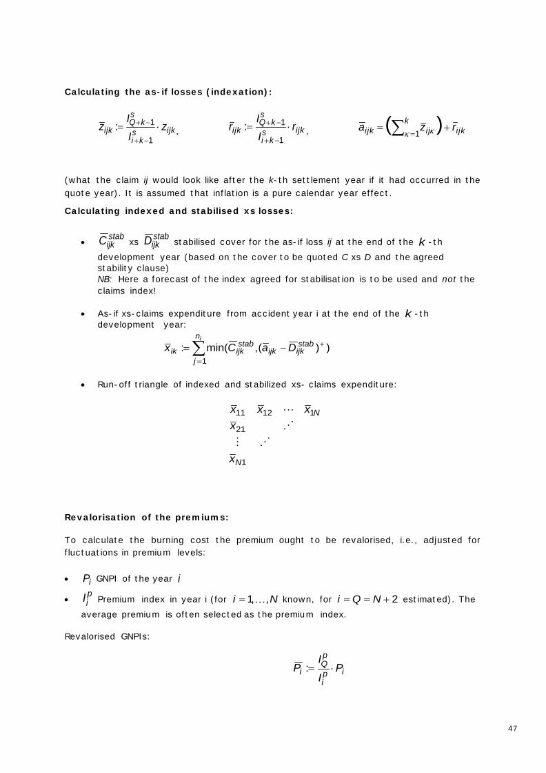
47
Calculating the as-if losses (indexation):
ijkski
skQ
ijk zII
z ⋅=−+
−+
1
1: , ijkski
skQ
ijk rII
r ⋅=−+
−+
1
1: , ∑ =+=
kijkiji jk rza
1)(
κ κ
(what the claim ij would look like after the k-th settlement year if it had occurred in the quote year). It is assumed that inflation is a pure calendar year effect.
Calculating indexed and stabilised xs losses:
• stabijkC xs stab
ijkD stabilised cover for the as-if loss ij at the end of the k -th development year (based on the cover to be quoted C xs D and the agreed stability clause) NB: Here a forecast of the index agreed for stabilisation is to be used and not the claims index!
• As-if xs-claims expenditure from accident year i at the end of the k -th development year:
∑=
+−=in
j
stabijkijk
stabijkik DaCx
1))(,min(:
• Run-off triangle of indexed and stabilized xs- claims expenditure:
1
21
11211
N
N
x
xxxx
Revalorisation of the premiums:
To calculate the burning cost the premium ought to be revalorised, i.e., adjusted for fluctuations in premium levels:
• iP GNPI of the year i
• piI Premium index in year i (for Ni ,,1= known, for 2+== NQi estimated). The
average premium is often selected as the premium index.
Revalorised GNPIs:
ipi
pQ
i PI
IP ⋅=:
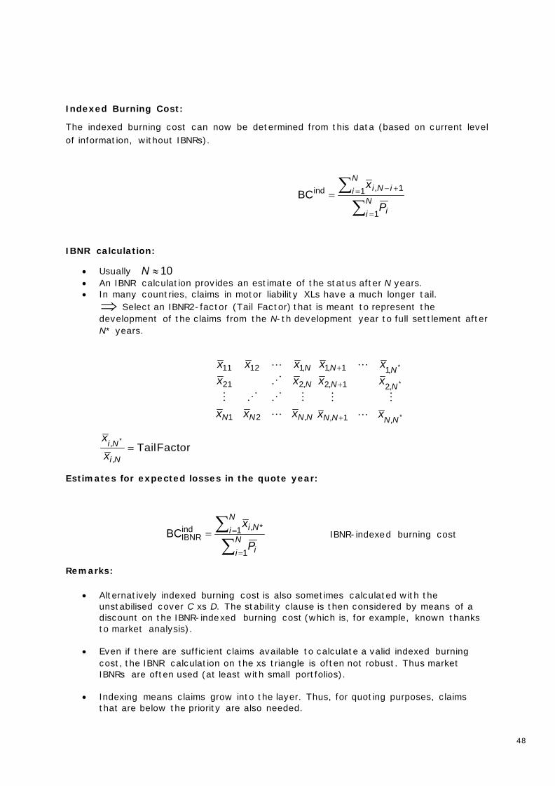
48
Indexed Burning Cost:
The indexed burning cost can now be determined from this data (based on current level of information, without IBNRs).
∑∑
=
= +−= N
i i
Ni iNi
P
x
1
1 1,indBC
IBNR calculation:
• Usually 10≈N • An IBNR calculation provides an estimate of the status after N years. • In many countries, claims in motor liability XLs have a much longer tail. ⇒ Select an IBNR2-factor (Tail Factor) that is meant to represent the development of the claims from the N-th development year to full settlement after N* years.
NNNN
N
N
xxx
xxxxx
,21
,221
,11211
*
*
*
,1,
,21,2
,11,1
NNNN
NN
NN
xx
xxxx
+
+
+
Factor Tail,
, *=
Ni
Nix
x
Estimates for expected losses in the quote year:
∑∑
=
== Ni i
Ni Ni
P
x
1
1 *,indIBNRBC IBNR-indexed burning cost
Remarks:
• Alternatively indexed burning cost is also sometimes calculated with the unstabilised cover C xs D. The stability clause is then considered by means of a discount on the IBNR-indexed burning cost (which is, for example, known thanks to market analysis).
• Even if there are sufficient claims available to calculate a valid indexed burning cost, the IBNR calculation on the xs triangle is often not robust. Thus market IBNRs are often used (at least with small portfolios).
• Indexing means claims grow into the layer. Thus, for quoting purposes, claims that are below the priority are also needed.

49
In the claims reporting clause a floor is defined above which claims have to be reported to the re-insurer (typically from 50% or 75% of the priority).
• For that part of the layer between the largest claim and the ceiling, an additional price should be factored in (e.g., extrapolation or exposure).
• If the period under observation contains an unusually high claim this is often spread over a longer period.
• The selection of the observation period is especially important:
- IBNR-problem and sufficient statistical basis ⇒ as long a period as possible
- High error risk in the as-if correction of old claims ⇒ as short a period as possible
In practice periods of observation of between seven and ten years are usually used.
• High significance of change risk:
- Deviations of actual claims inflation from forecast development of claims index
- Deviations from forecast development of stability index
• Sensitivity analyses enable change risk to be better assessed (e.g., consequence of superimposed inflation being one percentage point higher than expected …)
Practical consequence of various inflation assumptions / sensitivity analyses The following assumes for the model described above a notional fixed rate of inflation of 4.75 % for the future consisting of a 2.75 % increase in the wages and earnings index (LGI) and 2% hyperinflation for seriously ill or injured (SII).
This benchmark scenario is henceforth denoted as BM. If one assumes a reinsurance treaty with a stability clause based on the wages and earning index with a margin of 10% (APK 10), one gets, by varying the assumptions for the wages and earning index and the hyperinflation from the benchmark scenario, different results for the indexed and stabilized burning cost if 10 accident years and 10 subsequent years are taken into consideration. It is important to emphasis that, in this case, changes in the wages and earning index affect both the claims index and the index for the stability clause whereas changes in the hyperinflation only affect the claims index.
In the following table, the variations observed for the wages and earning index have been applied to the rows and the variations for hyperinflation applied to the columns. If one now assumes the following deviations from the benchmark scenario (BM), LGI 1.75% (instead of 2.75%, i.e., BM-1%) and hyperinflation 0.5% (instead of 2%, i.e., BM-1.5%), one gets as the indexed, stabilized 10-year burning cost xs 1 million precisely 86.4% of the value calculated with the benchmark scenario.
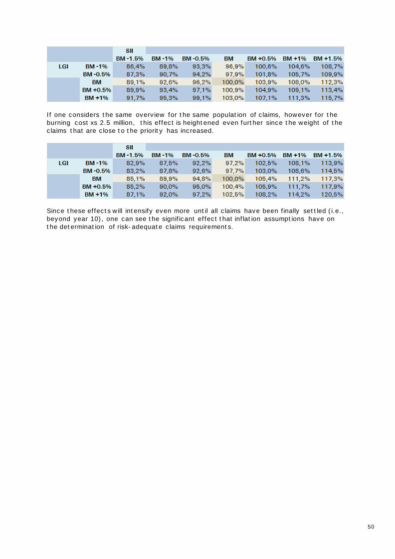
50
If one considers the same overview for the same population of claims, however for the burning cost xs 2.5 million, this effect is heightened even further since the weight of the claims that are close to the priority has increased.
Since these effects will intensify even more until all claims have been finally settled (i.e., beyond year 10), one can see the significant effect that inflation assumptions have on the determination of risk-adequate claims requirements.
51
4 Future development of interest rate and inflation
How are interest and inflation likely to develop in the future? This question has a material influence on actuarial calculations and projections, especially in the areas of
• Reserving: Inflation and discounting are key factors in determining best estimate reserves.
o In order to be able to analyse various possible developments, scenario analyses ought to be performed. This requires appropriate deterministic scenarios to be developed.
o If the actuarial reserve is to be posted in a balance sheet – for example the solvency balance sheet – then a concrete assumption about future inflation has to be made. This “expected” inflation scenario should be applied to the actuarially projected cash flow or rather this cash flow has to include this expected future inflation. Finally, this cash flow is usually discounted with a current yield curve in order to arrive at the current value of the best estimate reserve.
• Rating/Pricing: Inflation affects future claims expenditure. This must be considered in pricing.
• Internal modelling: Interest and inflation are risks that have a clear impact on the development of best estimate reserves and on claims expenditure in future years. The risks arising should be represented on the liabilities side of the internal model. To do so, stochastic yield curves and inflation scenarios have to be generated. This is largely a new discussion that has taken a considerable significance in the context of Solvency II. As a consequence of that inflation risk has to be taken into account as part of reserving risk. But can we even define inflation risk at all? And how can it be modelled?
This shows that, for the work of actuaries, the development of
• deterministic and • stochastic
interest and inflation scenarios is crucial.
This chapter aims to discuss how such scenarios can be generated. Using the example of claims reserving it will illustrate how scenario analyses with deterministic scenarios are performed. Moreover it will show how a “best estimate inflation scenario” as part of a “future inflation workshop” can be determined when accounting for best estimate reserves. The topic of inflation risk for internal modelling will also be discussed. Before doing so inflation risk will be defined before demonstrating how it can be modelled using stochastic scenarios.
4.1 Development of deterministic interest scenarios
In property/casualty insurance interest in used on the liabilities side of the balance sheet to discount technical cash flows. Thus, both interest scenarios and inflation scenarios are crucial when it comes to estimating future cash flow. In concrete terms “interest scenarios” usually mean scenarios for the yield curve used to discount premium, claims and reserves.
As a rule, many analyses and projections concerning the future development of interest or yield curves are available on the market. These are a good basis for the actuarial
52
reserve analysis as part of scenario analyses. Examples are the EIOPA yield curves to be used as part of Solvency II.
For the purposes of fair valuation, risk-free yield curves are used on the liabilities side. Nowadays of course, one has to ask what exactly “risk-free” means. Discussion of the potential default risks contained in government bonds, hitherto considered to be risk-free, is beyond the scope of this study.
4.2 Development of deterministic inflation scenarios
In claims reserving the following various forms of deterministic inflation assumptions are used:
• In the best estimate calculation, for example, for the Solvency II balance sheet or in accounting in general. This requires a single inflation scenario to be developed that then affects the projected cash flow and is thus incorporated in the balance sheet. That means that a decision has to be made about ONE scenario, so to speak a “best-estimate inflation scenario” that represents “the” expected level of inflation. Of course this expected level of inflation can contain various inflation assumptions for various types of claim. One must ensure that this one scenario is consistent, that it suits historic data, that it fits the assumed yield curve etc.
• Scenario analyses do not involve developing one single ideal scenario but rather testing the consequences of several different scenarios. Thus, several scenarios are developed. In so doing, every scenario is not required to be as exact as possible but rather a whole spectrum of possible scenarios is generated that may each produce very different results.
Both these aspects will be explored in greater detail below.
The requirements described above for reserving naturally also apply more or less to rating/pricing.
It must be noted that in standard reserving approaches implicit inflation embedded in the run-off triangle is projected in a certain way. When creating scenarios, one must thus always analyse and consider the effect of claims inflation that may go beyond the implicit inflation.
4.2.1 Inflation forecasting
In this study, the “best estimate inflation scenario” denotes “the” future expected level of inflation. This expectation depends to a great extent on the individual company, its business model and the Line of Business being observed. The scenario inevitably has a certain degree of subjectivity. Thus, expert judgement is very important.
In order to arrive at a solid, valid, transparent and understandable assessment, a separate appropriate process should be set up. The goal of this process is to assemble a panel of experts from different disciplines, to compare and coordinate their opinions and the results of their analyses so as to consolidate different correlating qualitative and quantitative effects of various factors into one “expected claims inflation level”.
Some companies have already set up processes of this type, giving them names such as
• Future Inflation Workshop; or • Task Force Future Inflation.
In this context we use the term “Inflation Forecasting”.

53
Below, we will outline one possible approach and the possible components of such a process. The design of such an inflation forecasting process will, of course, depend on the situation of the individual company and each company will make its own decision.
We will concentrate on the task of determining a “best estimate inflation scenario” for claims reserving of a given claims portfolio. This means that this scenario is to be used for determining the best estimate reserve for, for example, the solvency balance sheet. A similar approach could be applied to rating/pricing.
The basis for an inflation forecast should be solid and detailed data:
• Determining the historic inflation of the claims portfolios, for example, using the accident year or separation method
• Compiling historic data on interest and official inflation indices and sub-indices that are (causally) connected to the claims segment, e.g., CPI, CPI Transport, medical care, …
• Compiling historic data on the claims portfolio in the form of time series, e.g., the proportion of personal injury claims, the proportion of property claims, frequency, breakdown into size classes, the proportion of different benefits as part of the claims expenditure (compensation, medical treatment, nursing care costs, loss of earnings, …).
Comprehensive analyses are carried out using this data. The inflation forecast can essentially be done in one of two different ways:
• Either by direct forward projection of the observed times series to the claims portfolio inflation;
• or by linking the Line of Business inflation to explanatory factors such as official inflation indices, proportions of types of benefit, ….
The aim of these analyses must therefore be to perform and make available the evaluations necessary for both these methods. This certainly includes determining correlations, regression analyses and much more.
On the basis of these analyses a process of discussion can be initiated that will result in an estimation of the specific future inflation. This process will include the relevant experts such as:
• product managers • claims experts • economists • actuaries • investors
They will discuss:
• how the official factors (CPI, CPI Transport, …) will develop. • how the specifics (frequency, proportion of personal injury, proportion of types of
benefit, …) of the claims portfolio will develop • how specific claims inflation will develop purely on the basis of the “measured”
time series • etc.
The results of these discussions will finally be consolidated into a consistent picture. That means “the” inflation expectation will be constructed. Instead of developing one single scenario, as an alternative, for example, three possible scenarios can be generated. These can then be used to fix “the” scenario that will be used in best estimate reserving.
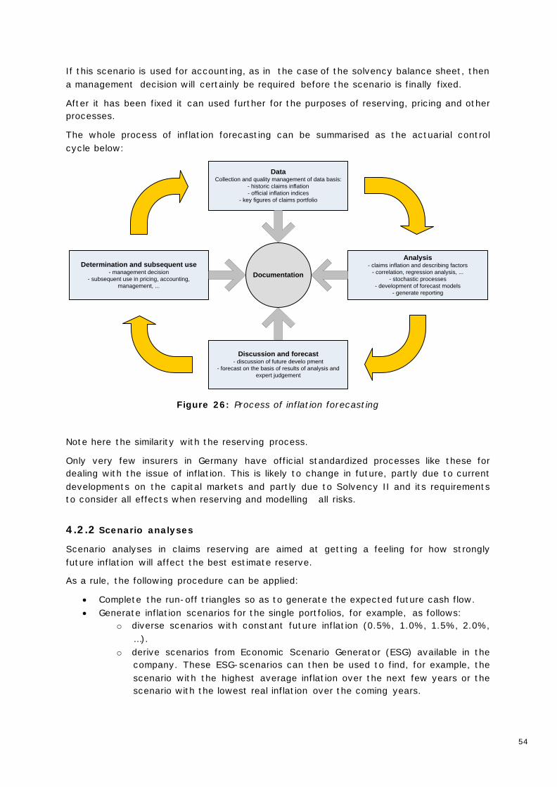
54
If this scenario is used for accounting, as in the case of the solvency balance sheet, then a management decision will certainly be required before the scenario is finally fixed.
After it has been fixed it can used further for the purposes of reserving, pricing and other processes.
The whole process of inflation forecasting can be summarised as the actuarial control cycle below:
DataCollection and quality management of data basis:
- historic claims inflation- official inflation indices
- key figures of claims portfolio
Analysis- claims inflation and describing factors
- correlation, regression analysis, ...- stochastic processes
- development of forecast models- generate reporting
Discussion and forecast- discussion of future develo pment
- forecast on the basis of results of analysis and expert judgement
Determination and subsequent use- management decision
- subsequent use in pricing, accounting, management, ...
Documentation
Figure 26: Process of inflation forecasting
Note here the similarity with the reserving process.
Only very few insurers in Germany have official standardized processes like these for dealing with the issue of inflation. This is likely to change in future, partly due to current developments on the capital markets and partly due to Solvency II and its requirements to consider all effects when reserving and modelling all risks.
4.2.2 Scenario analyses
Scenario analyses in claims reserving are aimed at getting a feeling for how strongly future inflation will affect the best estimate reserve.
As a rule, the following procedure can be applied:
• Complete the run-off triangles so as to generate the expected future cash flow. • Generate inflation scenarios for the single portfolios, for example, as follows:
o diverse scenarios with constant future inflation (0.5%, 1.0%, 1.5%, 2.0%, …).
o derive scenarios from Economic Scenario Generator (ESG) available in the company. These ESG-scenarios can then be used to find, for example, the scenario with the highest average inflation over the next few years or the scenario with the lowest real inflation over the coming years.
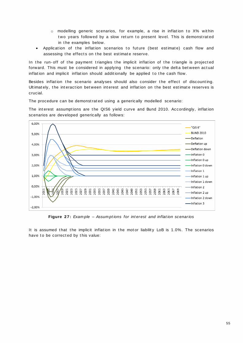
55
o modelling generic scenarios, for example, a rise in inflation to X% within two years followed by a slow return to present level. This is demonstrated in the examples below.
• Application of the inflation scenarios to future (best estimate) cash flow and assessing the effects on the best estimate reserve.
In the run-off of the payment triangles the implicit inflation of the triangle is projected forward. This must be considered in applying the scenario: only the delta between actual inflation and implicit inflation should additionally be applied to the cash flow.
Besides inflation the scenario analyses should also consider the effect of discounting. Ultimately, the interaction between interest and inflation on the best estimate reserves is crucial.
The procedure can be demonstrated using a generically modelled scenario:
The interest assumptions are the QIS6 yield curve and Bund 2010. Accordingly, inflation scenarios are developed generically as follows:
Figure 27: Example – Assumptions for interest and inflation scenarios
It is assumed that the implicit inflation in the motor liability LoB is 1.0%. The scenarios have to be corrected by this value:
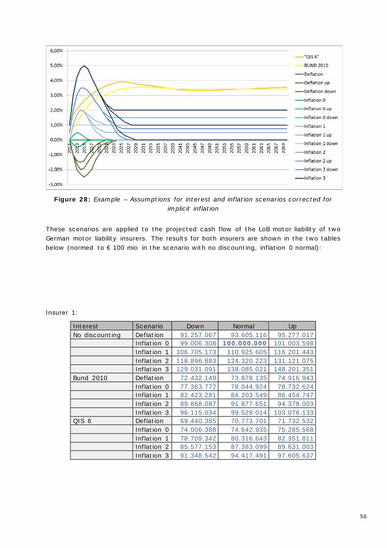
56
Figure 28: Example – Assumptions for interest and inflation scenarios corrected for implicit inflation
These scenarios are applied to the projected cash flow of the LoB motor liability of two German motor liability insurers. The results for both insurers are shown in the two tables below (normed to € 100 mio in the scenario with no discounting, inflation 0 normal):
Insurer 1:
Interest Scenario Down Normal Up No discounting Deflation 91.257.067 93.605.116 95.277.017 Inflation 0 99.006.308 100.000.000 101.003.598 Inflation 1 106.705.173 110.925.605 116.201.443 Inflation 2 118.896.883 124.320.223 131.121.075 Inflation 3 129.031.091 138.085.021 148.201.351 Bund 2010 Deflation 72.432.149 73.878.135 74.916.943 Inflation 0 77.363.772 78.044.924 78.732.624 Inflation 1 82.423.281 84.203.549 86.454.747 Inflation 2 89.868.087 91.877.651 94.378.003 Inflation 3 96.115.034 99.528.014 103.076.133 QIS 6 Deflation 69.440.385 70.773.701 71.732.532 Inflation 0 74.006.388 74.642.935 75.285.568 Inflation 1 78.709.342 80.316.643 82.351.811 Inflation 2 85.577.153 87.383.099 89.631.003 Inflation 3 91.348.542 94.417.491 97.605.637
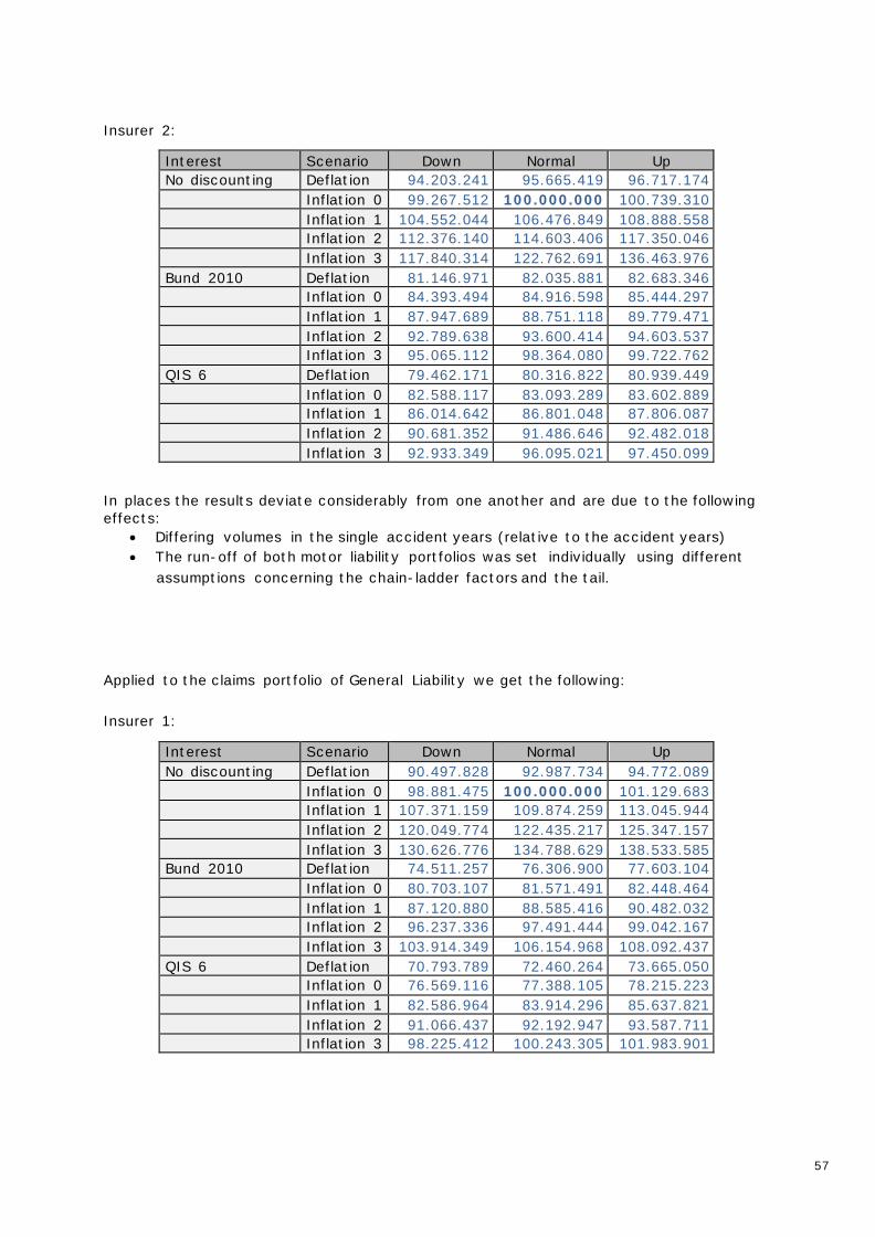
57
Insurer 2:
Interest Scenario Down Normal Up No discounting Deflation 94.203.241 95.665.419 96.717.174 Inflation 0 99.267.512 100.000.000 100.739.310 Inflation 1 104.552.044 106.476.849 108.888.558 Inflation 2 112.376.140 114.603.406 117.350.046 Inflation 3 117.840.314 122.762.691 136.463.976 Bund 2010 Deflation 81.146.971 82.035.881 82.683.346 Inflation 0 84.393.494 84.916.598 85.444.297 Inflation 1 87.947.689 88.751.118 89.779.471 Inflation 2 92.789.638 93.600.414 94.603.537 Inflation 3 95.065.112 98.364.080 99.722.762 QIS 6 Deflation 79.462.171 80.316.822 80.939.449 Inflation 0 82.588.117 83.093.289 83.602.889 Inflation 1 86.014.642 86.801.048 87.806.087 Inflation 2 90.681.352 91.486.646 92.482.018 Inflation 3 92.933.349 96.095.021 97.450.099
In places the results deviate considerably from one another and are due to the following effects:
• Differing volumes in the single accident years (relative to the accident years) • The run-off of both motor liability portfolios was set individually using different
assumptions concerning the chain-ladder factors and the tail. Applied to the claims portfolio of General Liability we get the following: Insurer 1:
Interest Scenario Down Normal Up No discounting Deflation 90.497.828 92.987.734 94.772.089 Inflation 0 98.881.475 100.000.000 101.129.683 Inflation 1 107.371.159 109.874.259 113.045.944 Inflation 2 120.049.774 122.435.217 125.347.157 Inflation 3 130.626.776 134.788.629 138.533.585 Bund 2010 Deflation 74.511.257 76.306.900 77.603.104 Inflation 0 80.703.107 81.571.491 82.448.464 Inflation 1 87.120.880 88.585.416 90.482.032 Inflation 2 96.237.336 97.491.444 99.042.167 Inflation 3 103.914.349 106.154.968 108.092.437 QIS 6 Deflation 70.793.789 72.460.264 73.665.050 Inflation 0 76.569.116 77.388.105 78.215.223 Inflation 1 82.586.964 83.914.296 85.637.821 Inflation 2 91.066.437 92.192.947 93.587.711 Inflation 3 98.225.412 100.243.305 101.983.901
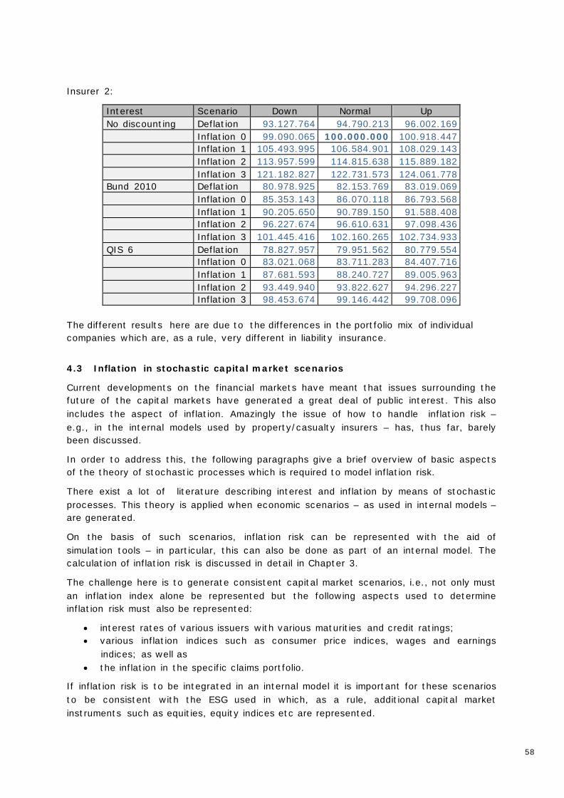
58
Insurer 2:
Interest Scenario Down Normal Up No discounting Deflation 93.127.764 94.790.213 96.002.169 Inflation 0 99.090.065 100.000.000 100.918.447 Inflation 1 105.493.995 106.584.901 108.029.143 Inflation 2 113.957.599 114.815.638 115.889.182 Inflation 3 121.182.827 122.731.573 124.061.778 Bund 2010 Deflation 80.978.925 82.153.769 83.019.069 Inflation 0 85.353.143 86.070.118 86.793.568 Inflation 1 90.205.650 90.789.150 91.588.408 Inflation 2 96.227.674 96.610.631 97.098.436 Inflation 3 101.445.416 102.160.265 102.734.933 QIS 6 Deflation 78.827.957 79.951.562 80.779.554 Inflation 0 83.021.068 83.711.283 84.407.716 Inflation 1 87.681.593 88.240.727 89.005.963 Inflation 2 93.449.940 93.822.627 94.296.227 Inflation 3 98.453.674 99.146.442 99.708.096
The different results here are due to the differences in the portfolio mix of individual companies which are, as a rule, very different in liability insurance.
4.3 Inflation in stochastic capital market scenarios
Current developments on the financial markets have meant that issues surrounding the future of the capital markets have generated a great deal of public interest. This also includes the aspect of inflation. Amazingly the issue of how to handle inflation risk – e.g., in the internal models used by property/casualty insurers – has, thus far, barely been discussed.
In order to address this, the following paragraphs give a brief overview of basic aspects of the theory of stochastic processes which is required to model inflation risk.
There exist a lot of literature describing interest and inflation by means of stochastic processes. This theory is applied when economic scenarios – as used in internal models – are generated.
On the basis of such scenarios, inflation risk can be represented with the aid of simulation tools – in particular, this can also be done as part of an internal model. The calculation of inflation risk is discussed in detail in Chapter 3.
The challenge here is to generate consistent capital market scenarios, i.e., not only must an inflation index alone be represented but the following aspects used to determine inflation risk must also be represented:
• interest rates of various issuers with various maturities and credit ratings; • various inflation indices such as consumer price indices, wages and earnings
indices; as well as • the inflation in the specific claims portfolio.
If inflation risk is to be integrated in an internal model it is important for these scenarios to be consistent with the ESG used in which, as a rule, additional capital market instruments such as equities, equity indices etc are represented.
59
The ESGs of various providers usually include many different scenarios concerning interest. Concerning inflation, however, the standard approach for scenarios tend to be restricted to the consumer price indices and wages and earnings indices for different regions. Inflation indices going beyond this – e.g., for medical inflation – are not usually included as standard in “normal” ESGs.
There are numerous providers of ESGs. The approaches they use to model inflation in connection with other capital market data are equally numerous. If inflation risk is to be represented in internal models, one must discuss
• whether and how data from own claims portfolios can and must be included in order to be able to represent specific inflation of the claims portfolio being investigated;
• what possibilities are provided by capital market scenario generators, or rather, the theory behind them, for modelling LoB-specific inflation;
• whether scenarios generated in this way realistically represent the phenomena and connections to other aspects of the capital markets that are observed in reality; and
• whether and how expectations concerning the future development of interest and inflation (expected values, variances, connections) can be incorporated and represented.
In general, a considerable degree of research and development effort is necessary to handle company-specific situations and requirements satisfactorily.
4.4 Stochastic processes to describe economic scenarios
If one considers the consistency between the economic scenarios described in the last paragraph, there are basically three inflation modelling requirements that an internal model should meet:
(1) Consistency with stochastic modelling of the yield curve (2) a. Modelling the realised inflation rates for future financial years
b. Modelling the inflation expectation at future points in time (3) Modelling company-specific claims inflation for different claims portfolios
This section will show two basic procedures that ensure (1) and (2) a. In this context a rough overview of interest and inflation models is given and it will be shown which approaches to modelling LoB-specific inflation could be adopted (3). In order to have a representation of the inflation risk for the actuary in the box approach it is necessary to calculate a conditional expectation (2)b in addition to ultimate inflation risk. This is discussed afterwards.
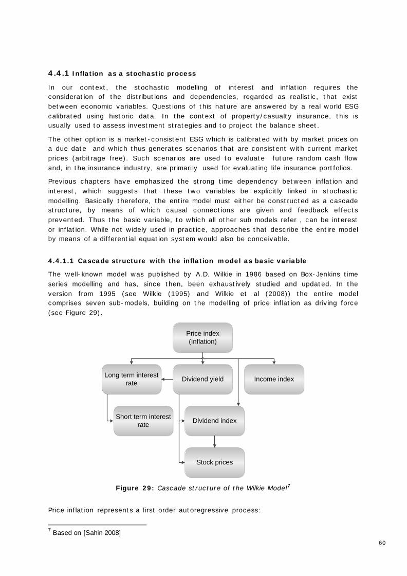
60
4.4.1 Inflation as a stochastic process
In our context, the stochastic modelling of interest and inflation requires the consideration of the distributions and dependencies, regarded as realistic, that exist between economic variables. Questions of this nature are answered by a real world ESG calibrated using historic data. In the context of property/casualty insurance, this is usually used to assess investment strategies and to project the balance sheet.
The other option is a market-consistent ESG which is calibrated with by market prices on a due date and which thus generates scenarios that are consistent with current market prices (arbitrage free). Such scenarios are used to evaluate future random cash flow and, in the insurance industry, are primarily used for evaluating life insurance portfolios.
Previous chapters have emphasized the strong time dependency between inflation and interest, which suggests that these two variables be explicitly linked in stochastic modelling. Basically therefore, the entire model must either be constructed as a cascade structure, by means of which causal connections are given and feedback effects prevented. Thus the basic variable, to which all other sub models refer , can be interest or inflation. While not widely used in practice, approaches that describe the entire model by means of a differential equation system would also be conceivable.
4.4.1.1 Cascade structure with the inflation model as basic variable
The well-known model was published by A.D. Wilkie in 1986 based on Box-Jenkins time series modelling and has, since then, been exhaustively studied and updated. In the version from 1995 (see Wilkie (1995) and Wilkie et al (2008)) the entire model comprises seven sub-models, building on the modelling of price inflation as driving force (see Figure 29).
Price index(Inflation)
Dividend yieldLong term interest rate Income index
Short term interest rate Dividend index
Stock prices
Figure 29: Cascade structure of the Wilkie Model7
Price inflation represents a first order autoregressive process:
7 Based on [Sahin 2008]
61
so that
Moreover:
with
Price index at time
Continuous change rate of price index from to
Expected value of
Standard deviation of
Autoregression parameter of .
If the autoregression parameter is less than 1, then the AR(1) process is at least weak stationary, i.e., expectation, variance and co-variance are time-invariant. As can be seen in Figure 29 , the long-term interest model builds on the price inflation model and the dividend yield model. In particular, the logarithmic long-term interest rate is modelled following subtraction of a future expected inflation rate as AR(1) process with the dividend yield as an additional component. With this the equation becomes:
with
Long-term interest rate at time
Inflation factor
MA process with continuous change rate of price inflation
AR process with additional effect of dividend yield
Expected value of .
Modelling of the short-term interest rate, too, is based on an AR(1) process in which the difference between the logarithmic long and short-term interest rates is considered. However, one must take into account that, in reality, short-term interest rates are, on average, lower than long-term rates. The following Wilkie equation takes this into account:
and
With
Short-term interest rate at time
Long-term interest rate at time

62
Expected value of
Autoregression parameter of
Standard deviation of .
For modelling of further variables, refer to the relevant financial mathematics literature.
Various aspects of the Wilkie model are criticised nowadays (see, e.g., Hibbert et al and Stahl et al). These are primarily the inadequate representation of the causality structures between the variables. In their model, which expanded the Wilkie model, Stahl et al, for example, considered additional significant correlations, e.g., between dividend index and purchasing powered-adjusted exchange rate. They were able to show the success of this model thanks to its improved forecasting quality.
4.4.1.2 Cascade structure with the interest model as basic variable
Instead of price inflation, the interest model (more precisely; yield curve model) in the overall model can precede in the causal chain.
Since the short rate (current rate, i.e., the interest rate for a secure investment for an infinitesimal short period of time) implies the whole yield curve, mathematical models to describe the future development of the yield curve using the short rate, so called short-rate models, are useful.
The best-known short-rate model is the Vasicek model (see Vasicek 1977), which uses a Gaussian Ornstein-Uhlenbeck process and is defined via a stochastic differential equation:
All other significant short-rate models are basically extensions of the Vasicek model, e.g.:
Cox-Ingersoll-Ross model (CIR):
Black-Karasinski model (BK):
with
short rate at time
long-term average of the short rate
mean-reversion parameter, strictly positive
standard deviation of
Wiener Process.
Short-rate models like this are simple to implement because they are one-factor models. The drift factor ensures that the interest rate reverts to the mean in the long
run with a speed dependent on . By integration of the short rate, the prices of zero
coupon bonds can be determined (and hence the entire yield curve).

63
One drawback of the Vasicek and the Hull & White models is that the short rate is normally distributed and hence negative interest rates are possible. CIR and BK excluded this by means of an - distribution and a lognormal distribution respectively. In general, one has to note that by the short rate an economic variable is modelled that cannot be observed on the capital market. The main reason for the change to other models is, however, that the above one-factor models imply that all interest rates in the yield curve are perfectly correlated and hence only a few realistic yield curve forms (normal, flat, inverse and irregular)can be generated.
One alternative is provided by including the forward rate, i.e., the interest rate that can be secured today for a specific point in time in the future. To this end, Heath-Jarrow-Morton developed a model framework that models the entire forward yield curve (hence forward-rate models). The forward rate, too, is an economic variable that cannot be observed on the capital market.
With this in mind market models use interest rates that can be observed on the capital markets, especially LIBOR rates in the LIBOR market model (LMM) or Brace-Gatarek-Musiela model (BGM) and swap rates in the swap market model.
The first of these multi-factor models can be described using the following equation:
with
Forward rate for time period
multi-dimensional Brownian motion.
By means of a principal component analysis the model keeps manageable in terms of the number of parameters.
This model, too, has a mean-reversion effect. Furthermore the distribution of the forward rates is lognormal, making the interest rates constantly positive. Moreover, in a multi-factor model such as this it is usually possible to reproduce 98% of the dynamic of realistic yield curve forms with only four factors. Adding further factors may result in an over parameterisation .
Note that the yield curve is normally projected for about 20 years. Afterwards, extrapolation using, for example, Nelson-Siegel functions, is necessary in order to include cash flow that is even further in the future. The “interface” between the modelled and extrapolated part of the yield curve remains, however, vulnerable to breaks or other inconsistencies.
Based on one of the interest models the rate of change of price inflation can, for example, be described by a linear autoregressive model with an autoregressive error term. This considers both short-term interest and the change in short-term interest:
rate of change of price inflation
short-term interest
heteroscedastic error term.
Such a model guarantees that, as has been observed historically, when inflation is high its volatility increases as well.
64
Despite the proven dependence between interest and inflation, the recent past has, triggered by the financial crisis, seen the difference between interest and price inflation shrink considerably or even become negative at several points in time and in several countries. It is difficult to capture such movements using the models referred to above. Models that represent economic cycles thus need further study in the future. Regime (State) switching models, for example, attempt to model drastic twists in the development of economic variables, accompanied by events such as financial crises or radical changes in government policy, using a random variable. This represents, depending on the development of the economic variables observed, the moment of regime switch.
4.4.1.3 Differences in the cascade structures
A cascade structure means that there are no interdependencies between the sub-models but rather a cause-effect relation. In Wilkie’s model, price inflation is causal for long and short-term interest; the interest is not causal for inflation. Conversely in the models discussed subsequently the short-term interest rate is causal for the price inflation; inflation is not causal for the interest. This requires the assumption that the model is exogenous which, as Stahl et al demonstrate, does not appear justified.
Furthermore, the above models are constructed in such a way that the cause is simultaneously accompanied by the effect; delayed causal effects cannot be usefully represented in this manner.
4.4.1.4 Wage and salary inflation
Studies have shown that wage and salary inflation lags behind price inflation. Thus it makes sense to model wage and salary inflation dependent on price inflation both at the same time and at the previous point in time.
The following well-known time series model is also a Wilkie model and consists of two components: the dependency on price inflation and an autoregressive process. The latter has the effect that, if wage and salary inflation is far away from the level that implies price inflation, this difference is not directly compensated for in the next time step.
Wilkie states:
so that
and
Δ
with
Wage and salary inflation at time
Continuous change in wage and salary inflation from to
Continuous change in price inflation from to
Expected value of
65
Autoregression parameter of
Standard deviation of
constant parameters
Δ Data frequency.
Several variations of the Wilkie model, e.g., concerning restricting the constant parameters, are discussed in the literature.
Basically the above model is an economical model, i.e., it has few parameters but still captures the wage and salary inflation cycle.
In this context the Philips curve is also mentioned; it was published in 1958 by A.W.H. Phillips and has been further developed since. It creates a relation between changes in nominal wages or rather prices and unemployment. The neo-Keynesian Philips curve is a model that captures future expected inflation (feed-forward mechanism). This contrasts with backward-looking adaptive models that use either MA processes or random walks (feed-backward mechanism).
4.4.1.5 Generating stochastic LoB-specific inflation indices
The necessity of generating inflation indices related to a company‘s own business was already described in the previous chapter. In so doing it is absolutely crucial that this is based on macro-economic variables, in particular interest, that come from the ESG. If this dependency is present, then the interdependency between the ESG variables guarantees an implicit dependency of the LoB-specific index to price and wage and salary inflation.
Generic modelling and parametrisation is not generally possible since LoB-specific inflation usually depends on the country and the product. Nevertheless we present some possible approaches here that can then be examined, extended and modified on a case by case basis.
The most intuitive option seems to be a linear combination of indices already available in the ESG, primarily price inflation, wage and salary inflation and gross domestic product (GDP), coupled with yield curves (if appropriate with different residual maturities):
With :
rate of change of LoB-specific inflation
rate of change of price inflation
rate of change of wage and salary inflation
rate of change of GDP
interest
constant term
error term (where possible, standard normally distributed though skewed distribution is also conceivable).
at time
66
A further possibility is a stochastic spread model based on the spread of the LoB-specific inflation to price or wage and salary inflation:
As an alternative to the additive version this model could also be made multiplicative, i.e., on the basis of relative spreads.
An Ornstein-Uhlenbeck process is appropriate for oscillating time series that, in the long run, revert to the expectation. To parametrise the equilibrium level, the continuity, the diffusion and the starting value can be determined by the maximum likelihood method .
Andrew Davidson & Co have developed a model for modelling the house price index that assumes that the house price index behaves like a dynamic asset similarly to a share index. Let:
with
logarithmic house price index at time
long-term expectation of
oscillating components
interest at time
long-term expectation of
standard deviation of .
In the above formula the drift component, which is dependent on the interest, represents the “affordability” of property; the oscillating component, defined using an Ornstein-Uhlenbeck process, represents the disequilibrium between supply and demand.
, as used in the above models, need not necessarily be the LoB-specific inflation. Initially an index could be modelled that is in addition to those indices present in the ESG, such as, for example, a medical inflation index, a construction costs index or a motor vehicle maintenance cost index. By mixing these additional indices (if possible together with ESG indices) it could be possible to produce the actual LoB-specific index although one would have to discuss whether, when mixing the indices, it would be useful to have an additional error term.
The need for an autoregressive component in modelling a LoB-specific index finally becomes apparent when considering expected inflation in future years. Without this, the level of previous inflation rates have no direct effect on the next inflation rate8, something which is usually undesirable .
Historic time series have to be used to parametrise the additional index, for example with the aid of regression analyses. These should represent the time series on which the parametrisation of the ESG is based as well as representing the time series that can be allocated to the additional index. Publicly available time series from the Bundesbank, the German Federal Statistical Office or Eurostat are suitable for this purpose. The greatest challenge arising when creating a LoB-specific inflation index is the need for a historic time series that represents inflation relating to the company’s own business. Chapter 2 8 Often submodels in the ESG have an autoregessive component meaning that the newly modelled inflation rate is definitely affected by the previous inflation rate. In practice, however, modelling has shown that this is usually insufficient and generates implausible results.

67
has already examined some possible ways to produce such an index. Likewise, sophisticated solutions are needed to handle sparse data and/or very noisy data. Possible solutions could be to smooth the data or to have the option of using individual judgement.
Although Chapter 3 has already concluded that, under normal circumstances, claims triangles should not be adjusted for inflation, legitimate application of the modelled stochastic LoB-specific inflation index nevertheless requires that this index is to be reduced by precisely that level of inflation that is already implicitly present in the stochastic projection because the claims triangles have not been de-inflated, i.e., adjusted for inflation.
4.4.2 Expected future inflation
To represent ultimate inflation risk in an internal model the previous section presented approaches for stochastically modelling realisations of future inflation. Taking another risk horizon into account it is, however, also important to represent one-year inflation risk in an internal model, which defines the risk of future adverse developments on individual future business years.
For stochastic modelling of reserve risk over a limited period, a virtual actuary, the so-called “actuary in the box” is often provided with the reserving methodology applied in t = 0; he then applies this to the additional claims experience in t=1, and subsequently proceeds in a same manner to the best-estimate reserving in . The claims experience gained is expressed in the model by a claims triangle which has been expanded by one (or several) diagonals.
Transferred to the issue of inflation this would mean determining inflation expectations every time re-reserving is done given previously observed inflation. Theoretically this would have to be accompanied by a re-parametrisation of the ESG every time re-reserving was done. This procedure is, however, unrealistic and different approaches need to be found.
In fact the ESG calibrated for the current time already implicitly provides the conditional expected inflation consistent with the interest rate: as the only economic variable in the ESG with a time structure the difference between nominal and real yield curve provides a kind of inflation yield curve and thus precisely the “price” of hedging against inflation:
Naturally inflation-linked bonds are not traded on the market and projected in ESGs for all different kinds of inflation and certainly not for LoB- and company-specific inflation. To model inflation expectations of such indices, other techniques are therefore necessary.
One modelling option consists in observing conditional expectation in the modelled “actual” rates of inflation. If, for example, after one year, one is in a scenario with high or low inflation, examining the realization of those scenarios that were similar in the first year provides an indicator of further inflation expectation.
Other approaches are also possible. For example, inflation expectation could consist in the actuary in the box assuming the approximation to the expected value of future inflation over a specific period.
68
4.5 Inflation risk in property / casualty insurance
What is inflation risk in property/casualty insurance? So far it has not been precisely defined. Also the question of the significance of inflation risk and how it can be calculated or modelled has rarely been discussed.
The following paragraphs will attempt to find some answers to these questions.
4.5.1 Fundamentals
Our starting point is the question: How and where does inflation have an effect in property/casualty insurance? We will restrict ourselves to the effects in “non-life” actuarial practice. There are certainly further areas where inflation may be important. One example is an insurer’s pension reserves for its own employees or the actuarial reserves for pension assets in liability lines (motor and general liability).
In our view, there are two key areas in non-life actuarial practice where inflation has an impact:
• In respect of reserves for incurred losses, i.e., for old accident years. Here there is the risk that, because of future inflation or rather a bad relation between interest and inflation, existing reserves will not be sufficient to meet obligations.
• In respect of the claims average for claims of the current or future accident year(s). Here there is the risk that premiums will not be sufficient to cover expenditure that has risen as a result of inflation.
Therefore, inflation risk is closely connected to premium risk or reserve risk and can, on the one hand, be considered as a component of these risks. On the other hand, however, it extends beyond these risks since we explicitly consider the effect of future changes in rates of inflation and interest. These effects can be significant and are directly connected to developments on the capital markets. This constitutes the bridge to the assets side of the balance sheet.
It could be tempting to state that inflation risk concerning previously incurred losses is contained in reserve risk. After all, inflation has already had an impact on the historic data in the run-off triangles. It would be fair to say that when calculating reserve risk – e.g., using the bootstrap method – volatility caused by inflation and hence inflation risk has already been represented. However, if a run-off triangle is adjusted for inflation the following effect is usually observed in practice: the volatility of the adjusted triangle (e.g., measured in terms of the standard deviation) is very similar to that of the unadjusted triangle – provided that the index series does not contain any significant breaks or jumps. Does this mean that the reserve risk in the unadjusted triangle corresponds to the reserve risk of the inflation-adjusted triangle and that the inflation risk can be ignored?
In our opinion the inflation risk is not zero. The stochastic effect of inflation on the best estimate reserves can be calculated explicitly: To do so one simply considers the projected expected future cash flow from the reserve run-off. This comprises the deterministic payments for the next years. If one applies stochastic scenarios for future inflationary changes to this deterministic cash flow, it is possible to directly see and calculate the volatility in the best-estimate reserve estimations caused by inflation.
This means that inflation risk is obviously not zero but the usual methods of determining reserve risk do not take it into consideration. The problem here is that, because of their underlying theory, these methods are not designed for measuring inflation risk. For example, methods usually work on the assumption that the triangle has been adjusted
69
for inflation. The diagonal effect of inflation usually only has a minimal effect on the volatility of the triangle.
As an interim conclusion one can say that inflation risk is an independent effect that needs to be considered as part of risk management. It is closely linked to reserve risk and premium risk. By extending traditional methods the risk can be determined at the same time as reserve and premium risk are being determined. The idea is to apply stochastic scenarios for interest and inflation to the stochastic claims cash flows generated by the usual bootstrapping methods.
4.5.2 Representing inflation risk in internal models
The basis for representing inflation risk in internal models is stochastic real world scenarios for inflation and yield curves. The following steps show one possible way of implementation. We assume an internal model that works on the basis of 100,000 simulations. The following input is required:
• 100,000 scenarios to realise the cash flow from the reserve run-off. • 100,000 scenarios for the ultimate claims expenditure of the new year. • The current risk-free yield curve (nominal interest rate), i.e., at time t=0. This is
required to discount the projected cash flow for the reserve run-off. • 100,000 scenarios risk-free yield curve (nominal interest rate), i.e., at time t=1.
This is required to discount the newly-simulated cash flow projections for the reserve run-off in time t=1.
• 100,000 scenarios for the rates of inflation in the official inflation indices in the next years, especially for
o Consumer Price Index o Wage and salary index o GDP deflator o MEDI o CPI Transport
These scenarios are then used to simulate the inflation specific to the respective claims portfolio using linear combination or similar.
• Alternatively, 100,000 scenarios directly for the rates of inflation specific to the respective claims portfolio in the next years. This means that these scenarios are generated by stochastic processes calibrated on own claims data.
• Scenarios for expected inflation for the next years in time t=1. For consumer price inflation, as described in the previous paragraph, this can be derived from the difference between nominal and real yield curves. Strictly speaking, however, one further step is necessary because, ultimately, expected inflation specific to the individual claims portfolio is required, see Section 4.4.2.
Care must be taken to ensure that these scenarios are consistent with one another, i.e., that within every simulation the inflation scenario is compatible with the corresponding interest scenario. If an ESG is used this can generally be assumed even if it will be difficult to prove for the user of the ESG. If, instead, an own construction is being used care should at least be taken that the correlations between the scenarios are realistic. Below we assume that scenarios from an ESG are available.
These scenarios are used in an internal model to generate 100,000 simulations of premium risk and reserve risk:
• Ultimate premium risk:
70
o The rate of inflation for period t=0 to t=1 is applied to the claim average of the respective claim amount distribution. This generates a volatility of the ultimate claims expenditure caused by inflation.
o If necessary, following the simulation of the ultimate claims expenditure for the current accident year the associated cash flow is generated. Then an inflation scenario can also be applied to this cash flow. Finally it is discounted with the yield curve at time t=1.
• Ultimate reserve risk: o For all of the 100,000 realisations of the cash flow of the reserve run-off, the
inflation scenario is applied according to a randomly drawn ESG scenario number. Finally it is discounted with the associated yield curve.
• One-year reserve risk: o The actuary in the box method is applied to project the cash flow in the
100,000 realisations of the diagonals of the run-off triangles including an inflation rate for the period t=0 to t=1. The scenario for expected inflation (assuming that inflation for the period t=0 to t=1 has occurred) is applied to each of the 100,000 cash flows from time t=1 according to the randomly drawn ESG scenario number. Finally the appropriate yield curve is used for discounting. The “actuary in the box” method is then continued as usual.
• One-year premium risk: o The one year premium risk is calculated on the basis of the method used for
one-year reserve risk. Inflation risk can be considered exactly as described above.
The ideas described here are basically new. Internal models will have to be developed further so as to reflect inflation risk.
In practice the main difficulty would appear to be the adequate representation of claims inflation using stochastic processes and their calibration. To date little experience of this is available. This is expected to change in the foreseeable future because representing inflation risk in an internal model will be a requirement that is certain to be supported by Solvency II.
71
5 Accounting and legal aspects
5.1 HGB (German GAAP)
5.1.1 Effects on liabilities
HGB norms were, in part, changed considerably by the German Act on the Modernisation of Accounting Law (BilMoG). The following aspects should be taken into account when it comes to inflation and interest fluctuations:
Provisions
Under § 253 paragraph 1 item 2 of HGB, provisions are to be assessed at the amount which is required to be paid according to a reasonable commercial assessment. This means, unlike previous assessment, that future price and cost increases have to be included (previously price and cost increases were assessed on the cut-off date).
In future, all provisions with a time to maturity of more than one year -- with the exception of technical provisions -- are to be discounted with an average market interest rate of the last 7 years appropriate for the remaining time to maturity (§ 253 para. 2).
Technical provisions
For technical provisions the existing procedure will be retained as set out in § 341e para. 1 HGB, i.e., provisions are to be valued based on the value on the balance sheet cut-off date and not discounted in accordance with § 253 para. 2.
Pension reserves
Pension reserves are generally valued at the discounted amount to be paid (see above).
The pension reserves to be created under BilMoG will be considerably higher because the underlying interest rate is well below the capitalisation rate of 6% which, for tax reasons, has regularly been used hitherto. Instead of determining individual discount rates for each individual obligation, it is permissible for both pension obligations and comparable long term obligations to assume a standardised residual maturity for all obligations of 15 years (e.g., 5.14% on 30.11.2011) (§ 253 para. 2 item 2).
German legislation has passed transitional rules allowing any deficits arising from amended valuation provisions to be allocated over a period of up to 15 years.
5.1.2 Effects on assets
Under BilMoG too, assets are generally valued at their acquisition cost or their lower market value. Two kinds of assets have to be considered separately.
• Securities held as current assets (i.e. securities that are not intended to be held long term) are valued according to strict lowest-value principle. This results in valuation haircuts arising from changes to market interest rates being reflected 100% on the asset side of the balance sheet. Later increases in value will be considered by means of write-ups to the amount of the original acquisition cost.
• Securities held as fixed assets (i.e. securities to be held longer term) are valued according to the moderate lowest-value principle. This means that valuation haircuts arising from changes to market interest rates are not reflected on the
72
assets side of the balance sheet, provided that a lasting value impairment need not be assumed.
The discount rate fixed bylaw is a seven-year average. Thus interest rate changes do not have an abrupt, but rather a gradual, effect on the liabilities side of the balance sheet. The moderate lowest-value principle means that changes in value arising from interest rate changes are countered, at least in the case of fixed-interest securities, even though capping write-ups to the level of acquisition cost means that a complete offset is not possible in the balance sheet.
5.2 IFRS
5.2.1 Effects on liabilities
Technical provisions
Accounting of insurance contracts at insurers is regulated in accordance with IFRS 4. The current version of IFRS 4 is a transitional standard that largely enables companies to retain their existing accounting practice.
Phase II of the IFRS 4 project (as at 2012) provides for technical provisions to be valued at the fulfilment value:
• Estimation of the statistical expected value of future company-specific cash flows including acquisition and administration costs as well as including future inflation.
• Discounting of the cash flows with current interest rates (risk-free market interest rates as at the cut off date, adjusted for a liquidity premium; use of yield curves, possible extrapolation of yield curves).
• A risk margin represents the risk that actual cash flows will exceed the fulfilment value.
• A residual margin (initial profit may not be reported) will be included in addition to the discounted expected value and risk margin at the beginning of the contract term; it equates to the expected profit and will be reduced over time.
Pension reserves (IAS 19)
Under IAS 19 pension reserves also have to be discounted by the interest rate prevailing on the cut-off date. In so doing, high quality underlying investments are assumed (usually corporate bonds with a AA rating). Discounting is done either using a yield curve or an average interest rate for a term of 15 years.
5.2.2 Effects on assets (IAS 39)
There are four asset categories; upon acquisition they are allocated to one of these asset categories:
Held to Maturity – Valuation is at the lower acquisition or market price provided that impairment is expected to be not permanent. Accordingly, interest rate fluctuations have no direct impact on the balance sheet and P&L statement.
Held for Trading or Fair Value through Profit and Loss - Interest rate fluctuations do have an impact on the balance sheet and P&L statement; market price or fair value approach.
73
Available for Sale – Interest rate fluctuations have no impact on the P&L statement but on the balance sheet
Loans and Receivables – Valuation is at amortised cost using the effective interest rate method to calculate the amortised cost (NB: amortisations required in the case of impairment that is expected to be permanent).
Outlook towards IFRS 9 (probable application in 2015)
IFRS 9 will replace IAS 39, in future valuation will only be done according to two asset categories:
Amortised Cost (valued at amortised acquisition cost)
Fair Value (valued at fair value).
Since their business models mean that insurers tend to invest conservatively most of their assets will be recognised in the accounts as amortised costs provided that the appropriate conditions are met. In order to steer the resulting mismatch risk resulting from the differing valuation methods insurers may still use the fair-value option and hedge accounting.
Against the backdrop of the discussion on the new version of IFRS 4, the introduction of a further asset category for the insurance industry is being considered. While not yet certain one of the above classes similar to 'available for sale' is being considered.
5.3 Solvency II
Under Article 78 of the Framework Directive, inflation must be taken into account when calculating technical provisions.
Moreover, Solvency II requires all material risks permanently to be taken into account. This applies especially to
• the ORSA process • the calculation of the SCR on the basis of an internal model.
Every insurer will therefore have to consider whether or not inflation constitutes a material risk for the company. It thus follows that inflation will have to be addressed as part of risk management.
Interestingly, inflation was not considered as a risk in the standard formula. This is made clear, for example, when one considers the calibration for reserve risk. The methods used do not include inflation risk as they are simply not suitable for doing so. Since the standard formula does not have a separate module for actuarial inflation risk either, this risk is quite simply ignored in the Solvency II standard formula. However, this may not be as serious as it appears since the factors for calibrating the standard formula were gauged extremely generously, and hence with security in mind, anyway. Certainly thanks to these many security buffers, inflation risk has been given implicit consideration.
In terms of methodology, however, this situation is not ideal. For it is now incumbent on every company once again to make its own separate observations and estimations concerning inflation risk. Moreover, every company has to judge on this basis whether or not the standard formula is appropriate for the company.
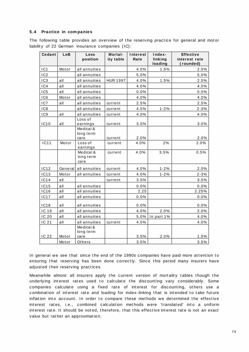
74
5.4 Practice in companies
The following table provides an overview of the reserving practice for general and motor liability of 22 German insurance companies (IC):
Cedant LoB Loss position
Mortal-ity table
Interest Rate
Index-linking loading
Effective interest rate (rounded)
IC1 Motor all annuities 4.0% 1.5% 2.5% IC2 all annuities 5.0% 5.0% IC3 all all annuities HUR 1997 4.0% 1.5% 2.5% IC4 all all annuities 4.0% 4.0% IC5 all all annuities 0.0% 0.0% IC6 Motor all annuities 4.0% 4.0% IC7 all all annuities current 2.5% 2.5% IC8 all annuities current 4.0% 1-2% 2-3% IC9 all all annuities current 4.0% 4.0%
IC10 all Loss of earnings current 3.0% 3.0%
Medical & long term care current 2.0% 2.0%
IC11 Motor Loss of earnings
current 4.0% 2% 2.0%
Medical & long term care
current 4.0% 3.5% 0.5%
IC12 General all annuities current 4.0% 1-2% 2.0% IC13 Motor all annuities current 4.0% 1-2% 2-3% IC14 all current 3.5% 3.5% IC15 all all annuities 0.0% 0.0% IC16 all all annuities 2.25 2.25% IC17 all all annuities 0.0% 0.0%
IC18 all all annuities 0.0% 0.0% IC 19 all all annuities 4.0% 2.0% 2.0% IC 20 all all annuities 5.0% In part 1% 4.0% IC 21 all all annuities current 4.0% 4.0%
IC 22 Motor
Medical & long term care 3.5% 2.0% 1.5%
Motor Others 3.5% 3.5%
In general we see that since the end of the 1990s companies have paid more attention to ensuring that reserving has been done correctly. Since this period many insurers have adjusted their reserving practices.
Meanwhile almost all insurers apply the current version of mortality tables though the underlying interest rates used to calculate the discounting vary considerably. Some companies calculate using a fixed rate of interest for discounting, others use a combination of interest rate and loading for index-linking that is intended to take future inflation into account. In order to compare these methods we determined the effective interest rates, i.e., combined calculation methods were 'translated' into a uniform interest rate. It should be noted, therefore, that this effective interest rate is not an exact value but rather an approximation.

75
The result is an average capitalisation interest rate of 2.6 %. The majority of companies surveyed (9) capitalise with a realistic to secure rate of 2-2.5 %. Five companies adopted an even safer reserving approach and either no longer discounted at all or used, at best, a minimal effective interest rate.
Five of the companies surveyed continue to reserve using a rate of 4-5%, which is rather 'tight'.
In addition to the interest rate and the mortality tables other factors can be used to evluate the quality of reserving, e.g., the initial values used for capitalisation, considering not yet secured liability quotients as well as possibly shorter life expectancy. These factors can transform safe reserves, at least considering the discounting interest rate used, into deficient ones.
76
6 Further aspects of interest rate and inflation
6.1 Pricing in primary insurance
The working group on pricing has published a study on the overall issue of calculation/pricing9. Its main conclusions concerning inflation are summarised as follows: All value-related figures are by definition affected by inflation, including cost developments. This also includes sums insured since, for example, reconstruction of a building after a total loss is dependent on wage and earnings developments. Indices are used here, too, (for example the construction prices index in residential buildings insurance) to automatically bring sums insured into line with current conditions.
This also applies when setting thresholds for large losses, which experience has shown are usually exceeded by considerably more losses within several years.
Sums insured and excesses / deductibles also suffer from the effects of inflation which can lead to their being 'devalued' if absolute sums have been selected.
In order to diagnose trends or the absence of trends, it is often appropriate to separate claims into claims frequency and average claim size. The underlying trends, which often only affect one of the two factors, are thus usually much more stable. The Average claims size should be adjusted for well-known inflation indices in order to establish or exclude residual trends if necessary.
Every forecast ought to take into account inflationary developments. This is particularly true when it comes to setting adequate reserves, with inflation in the healthcare sector deserving particular attention, for example.
In general, inflation clearly affects the validity of statistics.
Calculated premiums do not only depend on inflation but also on interest rate. The difference between the interest rate and the future inflation rate is critical.
6.2 Hedging against inflation
There are various options for hedging against the inflation risk to which technical reserves are exposed. Essentially, all one can expect is that the effects be mitigated since it is rarely possible to determine the level of inflation from the technical reserves, nor is it usually possible to match cover congruently in the market. Without demanding completeness , we will list some options and describe them in more detail below:
1. Investment in a capital market instrument that is directly linked to an inflation index.
2. Investment in a 'common' asset class with an observed or assumed (strong) negative correlation to inflation.
3. Implicit reinsurance solutions. 4. Explicit reinsurance solutions.
to 1.: In this case, so-called inflation-linked bonds (usually government bonds) are usually used with coupons and the nominal amount to be repaid partly depending on the development of an inflation index, as are various kinds of inflation swaps, i.e., OTC 9 See also [DGVM 38]
77
(over the counter) derivatives, which are derivative contracts in which one or more fixed payments -- fixed when the contract was entered into -- is/are swapped against one or more variable inflation-dependent payments. With the same underlying (i.e., underlying inflation index), the protection against inflation provided by these products is more or less identical, give or take a few minor details.
A liquid market exists for both swaps and Linkers albeit only with 'all-encompassing' inflation indices such as Eurostat Eurozone HICP Ex Tobacco and Unrevised Series NSA US CPI Urban Consumer NSA as the underlying indices. In this context, the question of basis risk and hence the efficiency of the hedging arises: in specific cases one has to evaluate how high the correlation is between 'actuarial' inflation and the indices mentioned, for example. Does hedging make sense or not? What is certain is that it will never be possible to achieve a 100% hedge using this method.
The advantage of swaps over inflation linkers is that this type of hedge does not require initial cash flow and thus does not require the portfolio to be restructured. One disadvantage, however, is that they can only be traded over the counter. For all these products, fair-value valuation is relatively simple since the market data required for the valuation are readily available and no complicated financial-mathematical models are required. For inflation swaps a different underlying is conceivable (such as for medical inflation) if a counterparty (bank) can be found for the variable side of the swap. However, it would be difficult to set a price as no market is available.
Since this hedging is not 100% efficient, the question of accounting treatment arises. Inflation linkers do not qualify as held-to-maturity. This means that any fluctuations in market value (including those arising from changes to interest rates) have to be represented in the equity capital or in the profit and loss (P&L) statement because the cash flow cannot be determined at the time of maturity. The real observable rates of inflation are basically reflected in the increase in the amortisation, meaning that every time an adjustment is made repayment will have to be recalculated. In other words, this means that no effects equating to the real level of inflation for the P&L statement of the corresponding year can be isolated. This means that, in accounting terms, there can be no protection in the same period even if the protection is available economically. Swaps must be accounted in trading, which would result in a market valuation in the P&L statement. This variation is thus superior to that of inflation-linked bonds especially if the fluctuations in the reserves caused by inflation can be booked simultaneously in the P&L statement.
to 2.: Hedging using shares, real estate and commodities:
As with Point 1, shares, real estate and commodities do not offer perfect protection against inflation. Over a very long period prices for all three of these asset classes will naturally rise (comparably with any inflationary movement), in the short term (< 5 years) no stable correlation of one of these asset classes with inflation has been observed historically (cf Swiss Re SIGMA Study10) meaning that investment purely for reasons of hedging against inflation appears to make little sense.
to 3.: Implicit (P&C) reinsurance solutions:
10 Swiss Re Sigma Study No 4/2010: “The impact of inflation on insurers”
78
Basic assumption: Inflation leads to an increase in future payments. Thus inflation should mainly affect the so-called long-tail lines of business. Below we present some solutions:
1. Non-proportional reinsurance: Non-proportional cover has significant exposure (from the reinsurer view) to inflation risk. This is caused by several factors, including much longer run-off periods and higher inflation in the case of larger losses (such as for serious personal injury claims, which almost always include a care cost component that is subject to increases in prices and rates). Typically this inflation risk is partly mitigated for reinsurers by means of so-called stabilisation clauses. The rationale is that inflation is spread proportionately between the primary and reinsurer. Only price increases beyond the wage and earnings index, so-called superimposed inflation, remains fully with the reinsurer. Hence, non-proportional reinsurance is only a partial hedge against inflation.
2. Quota share reinsurance: For quota share cessions, it is obvious that every increase in claims payments driven by inflation should be borne by both reinsurer and primary insurer at the agreed ratio.
3. Adverse development cover (ADC): This type of cover offers cover for losses that have occurred before cover commenced (typically very precisely restricted to specific industries and accident years). Its function can be compared to that of non-proportional reinsurance and it provides cover in case of run-off losses compared to the opening level of reserves at the signing of the treaty (assuming these exceed a predefined threshold above which the reinsurer is liable). Depending on the structure this type of cover may also include a stabilisation clause (see point 1).
4. Loss Portfolio Transfer (LPT): similarly to ADC, LPT covers losses that occurred before cover commenced. It works like quota share reinsurance and covers all movements in reserves up to complete run-off on a proportional basis. Therefore, in principle, the same applies as for quota share reinsurance above.
5. Multi-year cover: Multi-year covers provide reinsurance cover for a series of consecutive years on the basis of terms and conditions fixed in advance. This gives the reinsured additional cover against change risk (e.g., model changes; changes to the market environment). Normally multi-year covers contain so-called change of exposure clauses that are intended to ensure that the degree of exposure and hence the quality of cover remains homogenous over time. These clauses usually refer to changes in exposure such as, for example, with regard to the development of the aggregate liability / total sum insured, average premiums etc. Since the reinsurance cover for every single accident year is comparable with that of a one-year cover the same statement apply as made in the paragraphs above. If the expectation of future inflation for the series of covered years was not adequately considered in the price then this type of cover implicitly provides additional protection against inflation.
to 4.: Explicit solutions
1. "Enhance" reinsurance that implicitly provides cover against inflation: In rare cases, the above described cover models are enhanced to explicitly cover against inflation risk (the simplest case would be non-proportional cover with no stabilisation clause). In order to be able to provide this type of cover, the reinsurer breaks down the original risk into insurance risk and pure inflation risk (this is quite a challenge in practice). The cost of insuring against inflation is thus determined separately and then included in the overall price.

79
2. Hybrid cover: This type of reinsurance covers insurance risk similarly to classic reinsurance as well as additionally covering other risks, such as capital market risk, on the basis of selected indices. The rationale is that the adverse development of capital market indices is transferred to reinsurance cover parameters. This should increase the probability of using reinsurance cover given adverse capital market indices (trigger variable). One example of this would be a catastrophe cover whose priority is linked to a capital market index. Poor capital market performance lowers the priority of the cover since results on the investment side will probably suffer too, thus creating interest in better protection on the insurance side. In cases in which an inflation index or similar variable is used as a trigger variable there is additional protection against inflation. Typically, this kind of cover is used for industries with short run offs (i.e., property LoBs) on a one-year basis which, in turn, means this type of cover can only be used to hedge against inflation for short periods.
80
7 Inflation indices
Unless otherwise stated, all data in this chapter are taken from the website of the German Federal Statistical Office: www-genesis.destatis.de. Currently all indicators listed below refer to the base year 2005.
7.1 Prices
7.1.1 Consumer Price Index (CPI)
The reference population used to draw up consumer price statistics includes all providers of goods and services in the economic territory (domestic concept) whose goods and services form part of the consumer spending of private households. Spending on owner-occupied residential property is also included using the rental equivalent evaluation approach.
The reference population for goods, local units of all providers of goods and services, are determined on the basis of the Systematic Classification of Receipts and Expenditure of Private Households (SEA 98), which is in turn, based on the Classification of Individual Consumption by Purpose (COICOP).
Retail prices including value added tax and other consumer taxes for a representative selection of goods and services are collected. The information collected also includes the exact description of the good as well as other features that determine the price (e.g., type of business, warranty, method of dispatch, discounts, packaging, unit of quantity, payment terms).
The population of consumer price statistics consists of all sales of goods and services to private households in the economic territory. The sampling is done by means of a multi-stage procedure using the method commonly adopted in all price statistics of targeted selection of reporting communities, reporting offices and the actual goods and services for the price collection survey.
The current basket of goods (incl. weighting) contains: • Food and non-alcoholic drinks (103.55‰) • Alcoholic beverages, tobacco (38.99‰) • Clothing and footwear (48.88‰) • Housing, water, electricity, gas and other fuels (308.00‰) • Furniture, lighting equipment, appliances and other household equipment and
their maintenance (55.87‰) • Health (40.27‰) • Transport (131.90‰) • Communication (31.00‰) • Recreation, entertainment and culture (115.68‰) • Education (7.40‰) • Accommodation and restaurant services (43.99‰) • Miscellaneous goods and services (74.47‰)
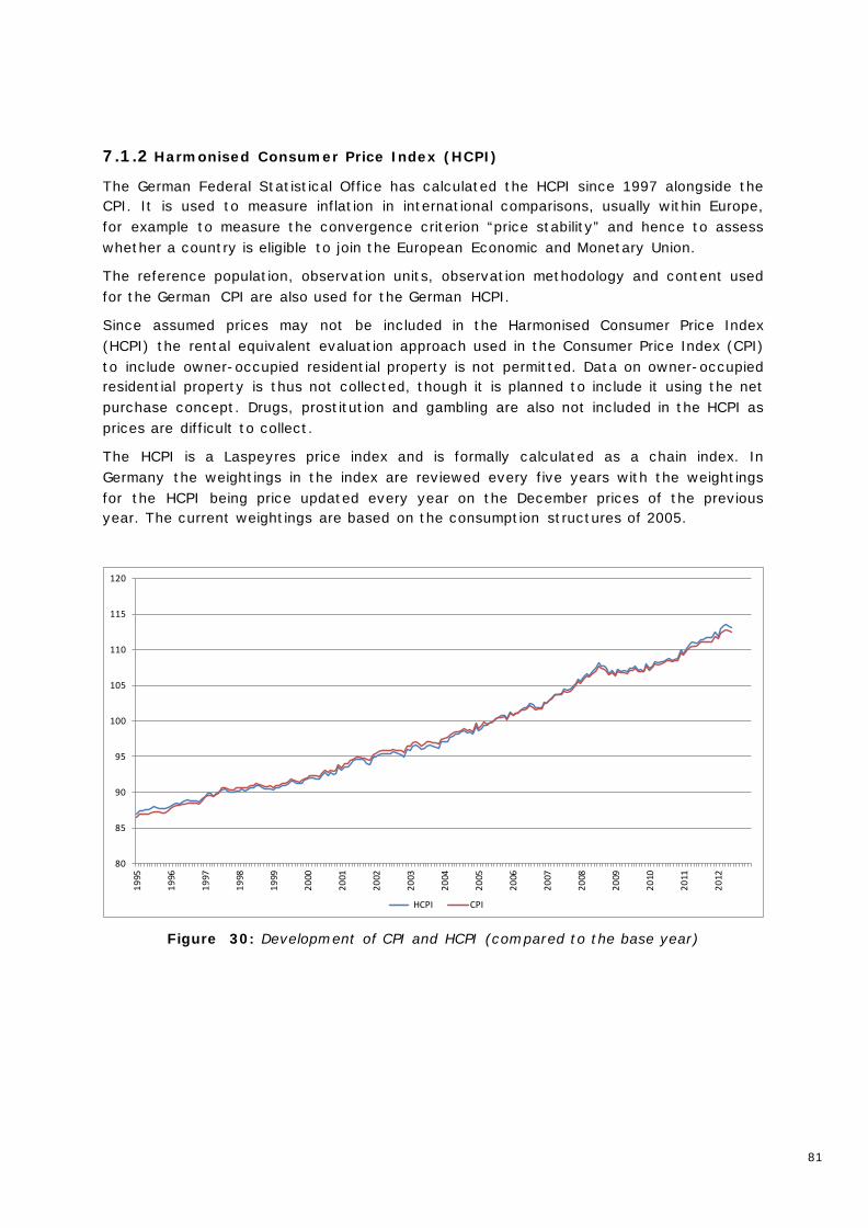
81
7.1.2 Harmonised Consumer Price Index (HCPI)
The German Federal Statistical Office has calculated the HCPI since 1997 alongside the CPI. It is used to measure inflation in international comparisons, usually within Europe, for example to measure the convergence criterion “price stability” and hence to assess whether a country is eligible to join the European Economic and Monetary Union.
The reference population, observation units, observation methodology and content used for the German CPI are also used for the German HCPI.
Since assumed prices may not be included in the Harmonised Consumer Price Index (HCPI) the rental equivalent evaluation approach used in the Consumer Price Index (CPI) to include owner-occupied residential property is not permitted. Data on owner-occupied residential property is thus not collected, though it is planned to include it using the net purchase concept. Drugs, prostitution and gambling are also not included in the HCPI as prices are difficult to collect.
The HCPI is a Laspeyres price index and is formally calculated as a chain index. In Germany the weightings in the index are reviewed every five years with the weightings for the HCPI being price updated every year on the December prices of the previous year. The current weightings are based on the consumption structures of 2005.
80
85
90
95
100
105
110
115
120
1995
1996
1997
1998
1999
2000
2001
2002
2003
2004
2005
2006
2007
2008
2009
2010
2011
2012
HCPI CPI
Figure 30: Development of CPI and HCPI (compared to the base year)
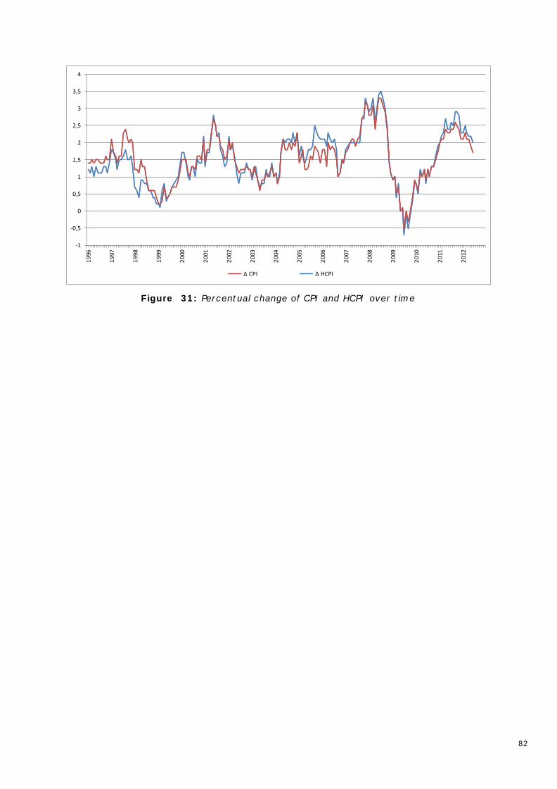
82
-1
-0,5
0
0,5
1
1,5
2
2,5
3
3,5
4
1996
1997
1998
1999
2000
2001
2002
2003
2004
2005
2006
2007
2008
2009
2010
2011
2012
∆ CPI ∆ HCPI
Figure 31: Percentual change of CPI and HCPI over time
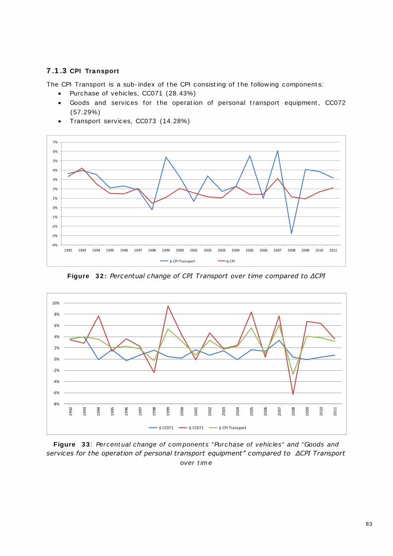
83
7.1.3 CPI Transport
The CPI Transport is a sub-index of the CPI consisting of the following components: • Purchase of vehicles, CC071 (28.43%) • Goods and services for the operation of personal transport equipment, CC072
(57.29%) • Transport services, CC073 (14.28%)
-4%
-3%
-2%
-1%
0%
1%
2%
3%
4%
5%
6%
7%
1992 1993 1994 1995 1996 1997 1998 1999 2000 2001 2002 2003 2004 2005 2006 2007 2008 2009 2010 2011
∆ CPI Transport ∆ CPI
Figure 32: Percentual change of CPI Transport over time compared to ∆CPI
-8%
-6%
-4%
-2%
0%
2%
4%
6%
8%
10%
1992
1993
1994
1995
1996
1997
1998
1999
2000
2001
2002
2003
2004
2005
2006
2007
2008
2009
2010
2011
∆ CC071 ∆ CC072 ∆ CPI Transport
Figure 33: Percentual change of components “Purchase of vehicles“ and “Goods and services for the operation of personal transport equipment” compared to ∆CPI Transport
over time
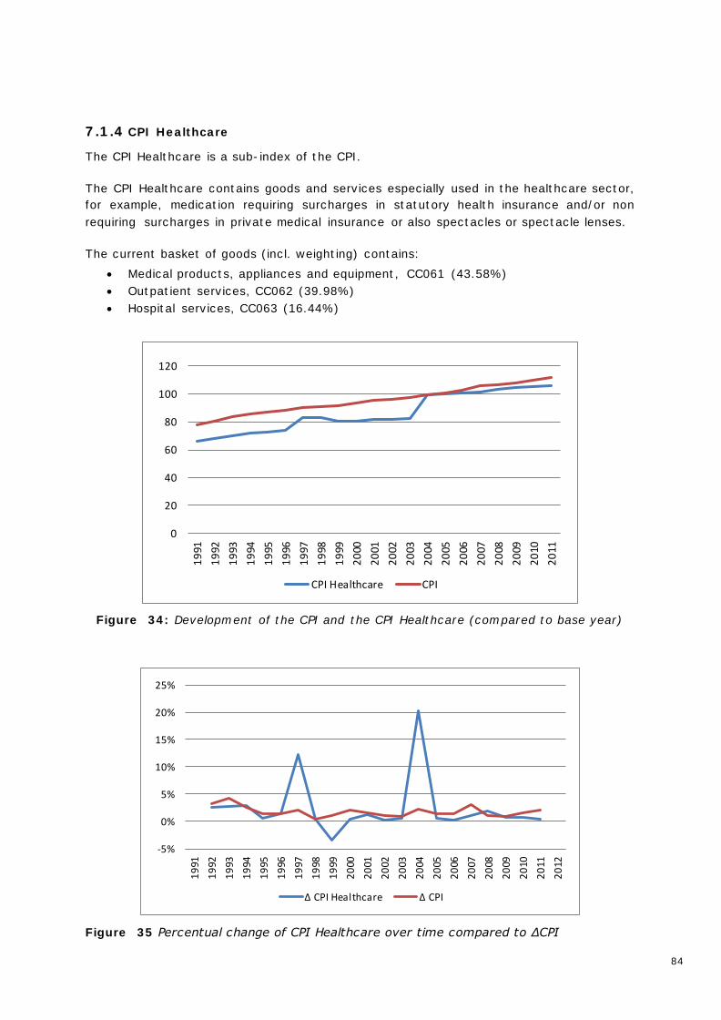
84
7.1.4 CPI Healthcare
The CPI Healthcare is a sub-index of the CPI.
The CPI Healthcare contains goods and services especially used in the healthcare sector, for example, medication requiring surcharges in statutory health insurance and/or non requiring surcharges in private medical insurance or also spectacles or spectacle lenses.
The current basket of goods (incl. weighting) contains: • Medical products, appliances and equipment, CC061 (43.58%) • Outpatient services, CC062 (39.98%) • Hospital services, CC063 (16.44%)
0
20
40
60
80
100
120
1991
1992
1993
1994
1995
1996
1997
1998
1999
2000
2001
2002
2003
2004
2005
2006
2007
2008
2009
2010
2011
CPI Healthcare CPI
Figure 34: Development of the CPI and the CPI Healthcare (compared to base year)
-5%
0%
5%
10%
15%
20%
25%
1991
1992
1993
1994
1995
1996
1997
1998
1999
2000
2001
2002
2003
2004
2005
2006
2007
2008
2009
2010
2011
2012
∆ CPI Healthcare ∆ CPI
Figure 35 Percentual change of CPI Healthcare over time compared to ∆CPI
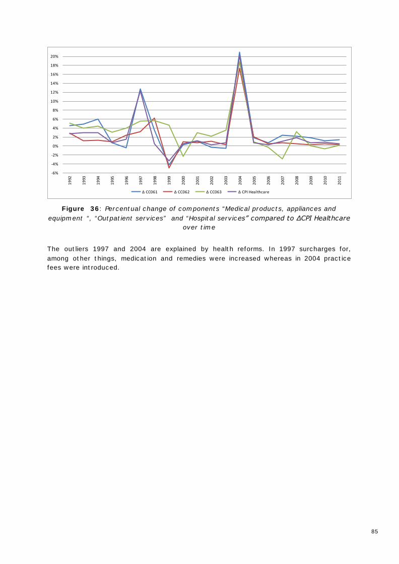
85
-6%
-4%
-2%
0%
2%
4%
6%
8%
10%
12%
14%
16%
18%
20%
1992
1993
1994
1995
1996
1997
1998
1999
2000
2001
2002
2003
2004
2005
2006
2007
2008
2009
2010
2011
∆ CC061 ∆ CC062 ∆ CC063 ∆ CPI Healthcare
Figure 36: Percentual change of components “Medical products, appliances and equipment “, “Outpatient services” and “Hospital services” compared to ∆CPI Healthcare
over time
The outliers 1997 and 2004 are explained by health reforms. In 1997 surcharges for, among other things, medication and remedies were increased whereas in 2004 practice fees were introduced.
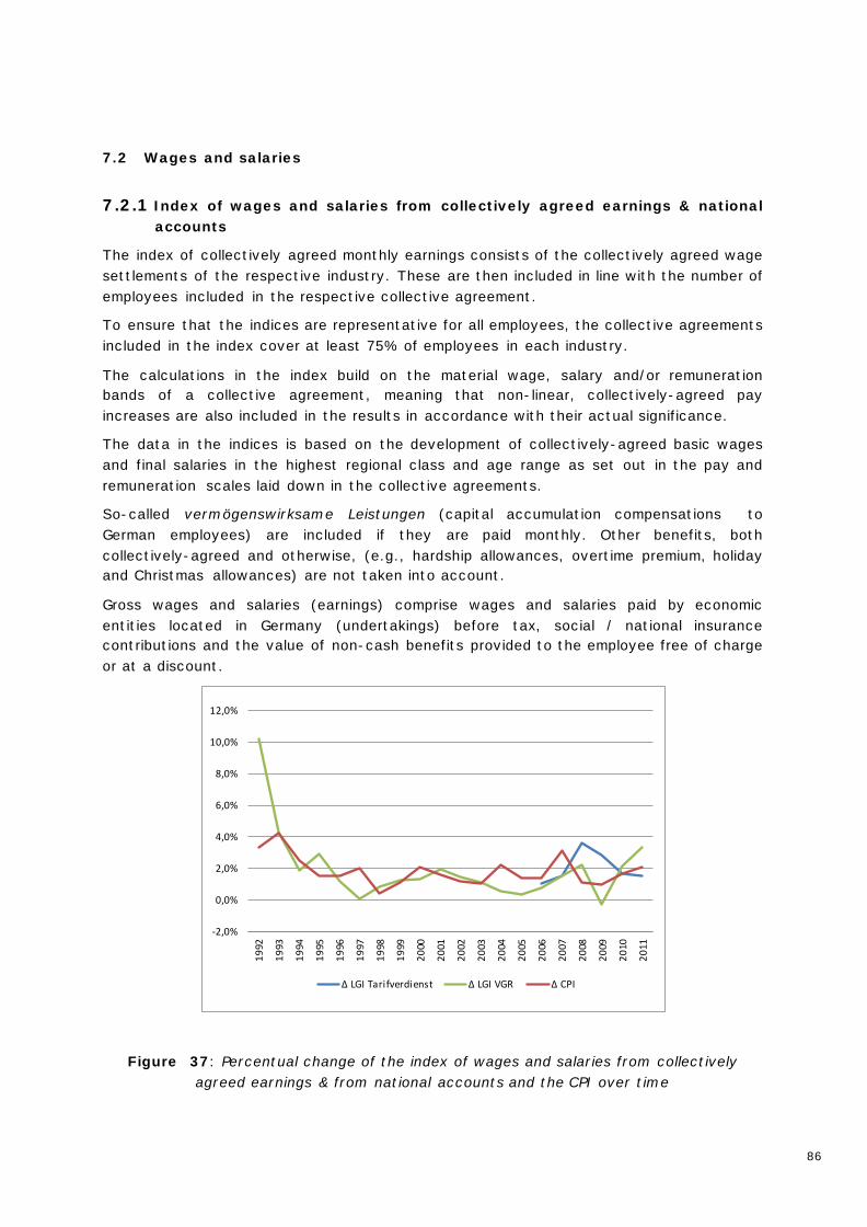
86
7.2 Wages and salaries
7.2.1 Index of wages and salaries from collectively agreed earnings & national accounts
The index of collectively agreed monthly earnings consists of the collectively agreed wage settlements of the respective industry. These are then included in line with the number of employees included in the respective collective agreement.
To ensure that the indices are representative for all employees, the collective agreements included in the index cover at least 75% of employees in each industry.
The calculations in the index build on the material wage, salary and/or remuneration bands of a collective agreement, meaning that non-linear, collectively-agreed pay increases are also included in the results in accordance with their actual significance.
The data in the indices is based on the development of collectively-agreed basic wages and final salaries in the highest regional class and age range as set out in the pay and remuneration scales laid down in the collective agreements.
So-called vermögenswirksame Leistungen (capital accumulation compensations to German employees) are included if they are paid monthly. Other benefits, both collectively-agreed and otherwise, (e.g., hardship allowances, overtime premium, holiday and Christmas allowances) are not taken into account.
Gross wages and salaries (earnings) comprise wages and salaries paid by economic entities located in Germany (undertakings) before tax, social / national insurance contributions and the value of non-cash benefits provided to the employee free of charge or at a discount.
-2,0%
0,0%
2,0%
4,0%
6,0%
8,0%
10,0%
12,0%
1992
1993
1994
1995
1996
1997
1998
1999
2000
2001
2002
2003
2004
2005
2006
2007
2008
2009
2010
2011
∆ LGI Tarifverdienst ∆ LGI VGR ∆ CPI
Figure 37: Percentual change of the index of wages and salaries from collectively agreed earnings & from national accounts and the CPI over time
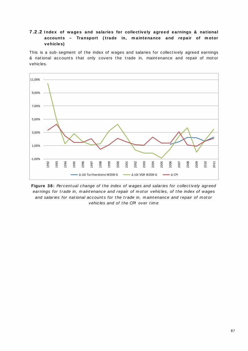
87
7.2.2 Index of wages and salaries for collectively agreed earnings & national accounts – Transport (trade in, maintenance and repair of motor vehicles)
This is a sub-segment of the index of wages and salaries for collectively agreed earnings & national accounts that only covers the trade in, maintenance and repair of motor vehicles.
-1,00%
1,00%
3,00%
5,00%
7,00%
9,00%
11,00%
1992
1993
1994
1995
1996
1997
1998
1999
2000
2001
2002
2003
2004
2005
2006
2007
2008
2009
2010
2011
∆ LGI Tarifverdienst WZ08-G ∆ LGI VGR WZ08-G ∆ CPI
Figure 38: Percentual change of the index of wages and salaries for collectively agreed earnings for trade in, maintenance and repair of motor vehicles, of the index of wages and salaries for national accounts for the trade in, maintenance and repair of motor
vehicles and of the CPI over time
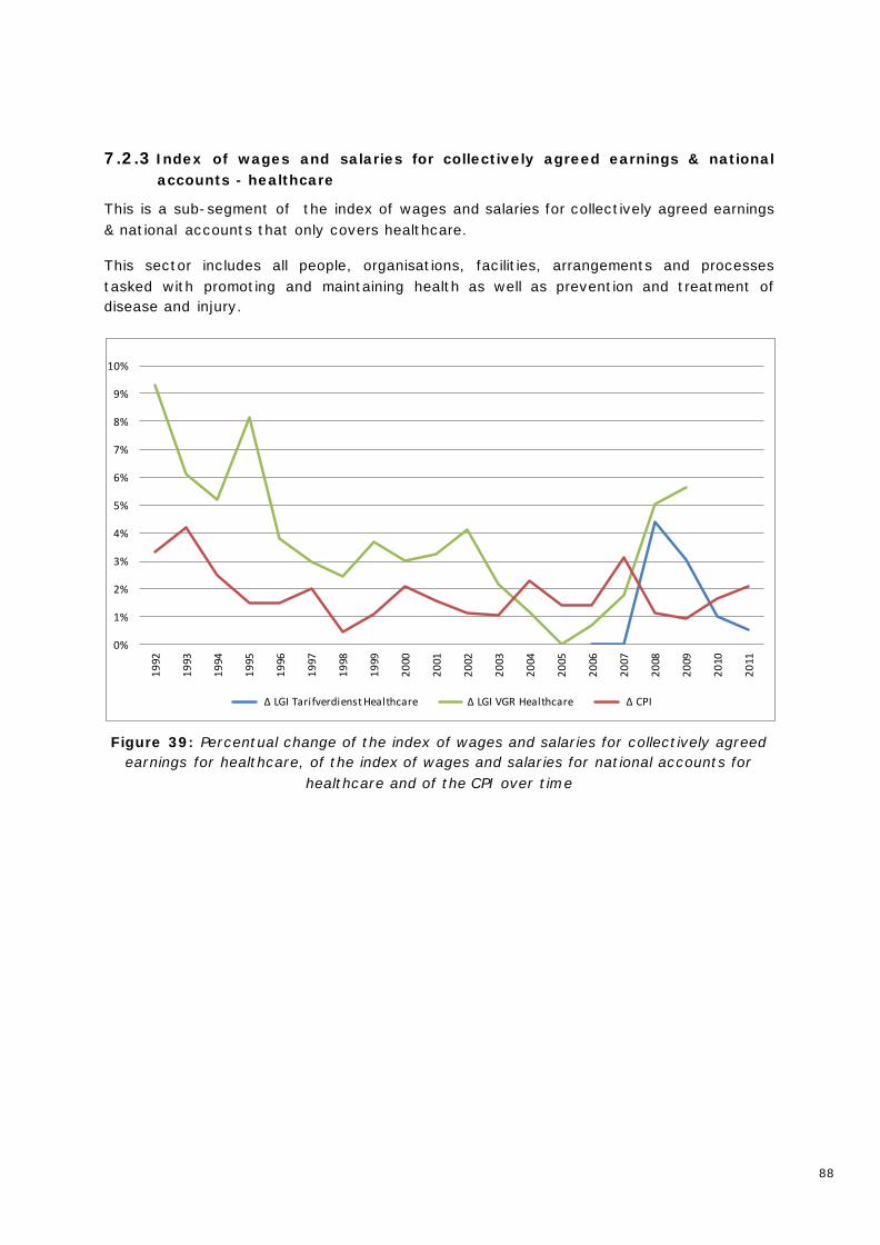
88
7.2.3 Index of wages and salaries for collectively agreed earnings & national accounts - healthcare
This is a sub-segment of the index of wages and salaries for collectively agreed earnings & national accounts that only covers healthcare.
This sector includes all people, organisations, facilities, arrangements and processes tasked with promoting and maintaining health as well as prevention and treatment of disease and injury.
0%
1%
2%
3%
4%
5%
6%
7%
8%
9%
10%
1992
1993
1994
1995
1996
1997
1998
1999
2000
2001
2002
2003
2004
2005
2006
2007
2008
2009
2010
2011
∆ LGI Tarifverdienst Healthcare ∆ LGI VGR Healthcare ∆ CPI
Figure 39: Percentual change of the index of wages and salaries for collectively agreed earnings for healthcare, of the index of wages and salaries for national accounts for
healthcare and of the CPI over time
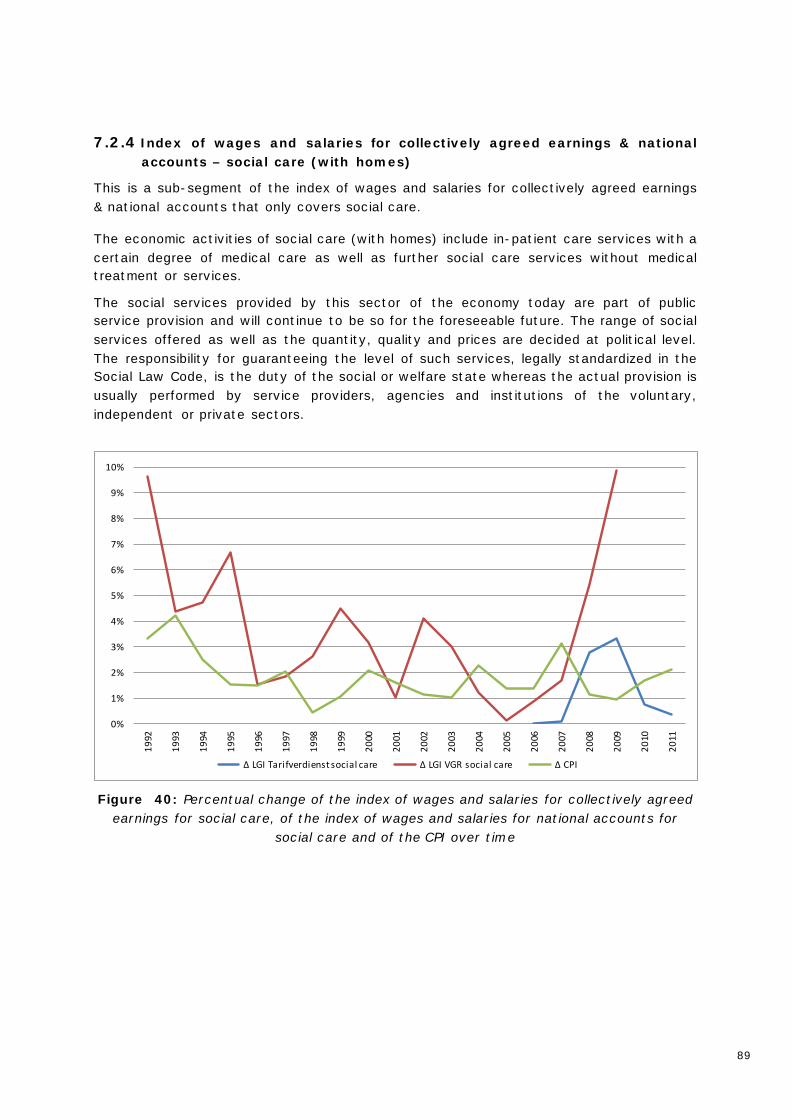
89
7.2.4 Index of wages and salaries for collectively agreed earnings & national accounts – social care (with homes)
This is a sub-segment of the index of wages and salaries for collectively agreed earnings & national accounts that only covers social care.
The economic activities of social care (with homes) include in-patient care services with a certain degree of medical care as well as further social care services without medical treatment or services.
The social services provided by this sector of the economy today are part of public service provision and will continue to be so for the foreseeable future. The range of social services offered as well as the quantity, quality and prices are decided at political level. The responsibility for guaranteeing the level of such services, legally standardized in the Social Law Code, is the duty of the social or welfare state whereas the actual provision is usually performed by service providers, agencies and institutions of the voluntary, independent or private sectors.
0%
1%
2%
3%
4%
5%
6%
7%
8%
9%
10%
1992
1993
1994
1995
1996
1997
1998
1999
2000
2001
2002
2003
2004
2005
2006
2007
2008
2009
2010
2011
∆ LGI Tarifverdienst social care ∆ LGI VGR social care ∆ CPI
Figure 40: Percentual change of the index of wages and salaries for collectively agreed earnings for social care, of the index of wages and salaries for national accounts for
social care and of the CPI over time
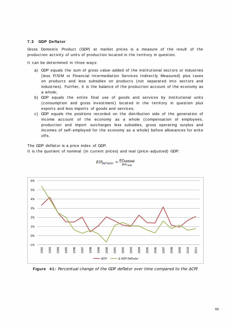
90
7.3 GDP Deflator
Gross Domestic Product (GDP) at market prices is a measure of the result of the production activity of units of production located in the territory in question.
It can be determined in three ways:
a) GDP equals the sum of gross value-added of the institutional sectors or industries (less FISIM or Financial Intermediation Services Indirectly Measured) plus taxes on products and less subsidies on products (not separated into sectors and industries). Further, it is the balance of the production account of the economy as a whole;
b) GDP equals the entire final use of goods and services by institutional units (consumption and gross investment) located in the territory in question plus exports and less imports of goods and services;
c) GDP equals the positions recorded on the distribution side of the generation of income account of the economy as a whole (compensation of employees, production and import surcharges less subsidies, gross operating surplus and incomes of self-employed for the economy as a whole) before allowances for write offs.
The GDP deflator is a price index of GDP. It is the quotient of nominal (in current prices) and real (price-adjusted) GDP:
-1%
0%
1%
2%
3%
4%
5%
6%
1992
1993
1994
1995
1996
1997
1998
1999
2000
2001
2002
2003
2004
2005
2006
2007
2008
2009
2010
2011
∆CPI ∆ GDP-Deflator
Figure 41: Percentual change of the GDP deflator over time compared to the ∆CPI
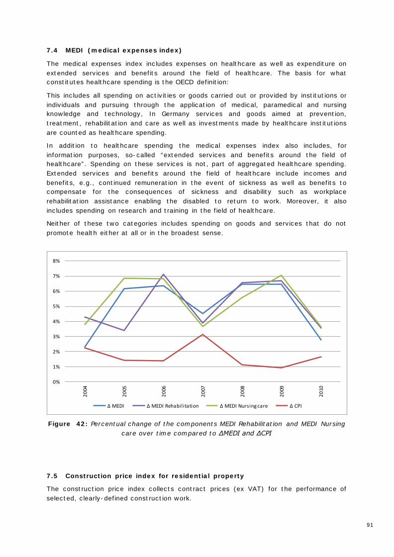
91
7.4 MEDI (medical expenses index)
The medical expenses index includes expenses on healthcare as well as expenditure on extended services and benefits around the field of healthcare. The basis for what constitutes healthcare spending is the OECD definition:
This includes all spending on activities or goods carried out or provided by institutions or individuals and pursuing through the application of medical, paramedical and nursing knowledge and technology, In Germany services and goods aimed at prevention, treatment, rehabilitation and care as well as investments made by healthcare institutions are counted as healthcare spending.
In addition to healthcare spending the medical expenses index also includes, for information purposes, so-called “extended services and benefits around the field of healthcare”. Spending on these services is not, part of aggregated healthcare spending. Extended services and benefits around the field of healthcare include incomes and benefits, e.g., continued remuneration in the event of sickness as well as benefits to compensate for the consequences of sickness and disability such as workplace rehabilitation assistance enabling the disabled to return to work. Moreover, it also includes spending on research and training in the field of healthcare.
Neither of these two categories includes spending on goods and services that do not promote health either at all or in the broadest sense.
0%
1%
2%
3%
4%
5%
6%
7%
8%
2004
2005
2006
2007
2008
2009
2010
∆ MEDI ∆ MEDI Rehabilitation ∆ MEDI Nursing care ∆ CPI
Figure 42: Percentual change of the components MEDI Rehabilitation and MEDI Nursing care over time compared to ∆MEDI and ∆CPI
7.5 Construction price index for residential property
The construction price index collects contract prices (ex VAT) for the performance of selected, clearly-defined construction work.
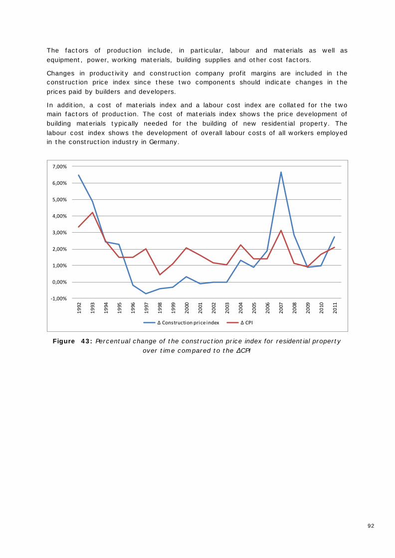
92
The factors of production include, in particular, labour and materials as well as equipment, power, working materials, building supplies and other cost factors.
Changes in productivity and construction company profit margins are included in the construction price index since these two components should indicate changes in the prices paid by builders and developers.
In addition, a cost of materials index and a labour cost index are collated for the two main factors of production. The cost of materials index shows the price development of building materials typically needed for the building of new residential property. The labour cost index shows the development of overall labour costs of all workers employed in the construction industry in Germany.
-1,00%
0,00%
1,00%
2,00%
3,00%
4,00%
5,00%
6,00%
7,00%
1992
1993
1994
1995
1996
1997
1998
1999
2000
2001
2002
2003
2004
2005
2006
2007
2008
2009
2010
2011
∆ Construction price index ∆ CPI
Figure 43: Percentual change of the construction price index for residential property over time compared to the ∆CPI

93
8 Bibliography
Chapter 1
Dowling & Partners Securities LLC (2009). Inflation is “Good” for (Re)Insurers Unless Expectations Change Suddenly & Materially. IBNR weekly July 24th (#29, Vol. XVI – Page 3)
Chapter 2
Baßeler, U., Heinrich, J., Utecht, B. (2010). Grundlagen und Probleme der Volkswirtschaft. Schäffer-Poeschel BWLhelfer.de. Inflation. bwlhelfer.de/html/Inflation.html www-genesis.destatis.de Kronberger, R. (2010). Inflation - Wird hohe Inflation wieder zum Thema? unet.fh-vie.ac.at/ralf.kronberger/aws_aktuelle_65_screen.pdf www.oecd.org Pätzold, J. (2008). Stabilisierungspolitik. Vahlen Verlag, Stuttgart Pätzold, J. Das Inflationsproblem. Ursachen und Strategien. www.juergen-paetzold.de/stabpol/BG+Infl/Inf lation.html Pohl, R. (1981). Theorie der Inflation – Grundzüge der monitären Makroökonomie. Franz Vahlen Verlag, München Riese, H. (1986). Theorie der Inflation. J. C. B. Mohr Verlag, Tübingen Chapter 3
www.genesis.destatis.de Radtke, M., Schmidt, K. D. (2004). Handbuch zur Schadenreservierung. Verlag Versicherungswirtschaft Karlsruhe Chapter 4
Albrecht, P. (2007). Grundprinzipien der Finanz- und Versicherungsmathematik. Schäffer-Poeschel. Albrecht, P., Maurer, R. (2008). Investment und Risikomanagement: Modell, Methoden, Anwendungen. Schäffer-Poeschel. Castle, J.L. Checking the Robustness and Validity of Model Selection: An Application to UK Wages. http://www.economics.ox.ac.uk/members/jennifer.castle/JLC_JobMarketPaper.pdf

94
Hamilton, J.D. (2005). Regime-Switching Models. http://dss.ucsd.edu/~jhamilto/palgrav1.pdf Hibbert, J., Mowbray, P., Turnbull, C. (2001). A stochastic asset model & calibration for long-term financial planning purposes. http://www.actuaries.org.uk/system/files/documents/pdf/hibbert0.pdf Levin, A. (2008), Andrew Davidson & Co. AD&Co’s Home Price Simulator. The Pipeline Levin, A. (2009), Andrew Davidson & Co. Geographical HPA Modeling and Forecasting. The Pipeline Stahl, G., Sibbertsen, P., Bertram, P. Modellrisiko = Spezifikation + Validierung. http://www3.wiwi.uni-hannover.de/Forschung/Diskussionspapiere/dp-468.pdf Wilkie, A.D. (1995). More on a stochastic asset model for actuarial use. British Actuarial Journal Wilkie, A.D., Sahin, S., Cairns, A., Kleinow, T. (2008). Revisiting the Wilkie investment model. http://www.actuaries.org/AFIR/Colloquia/Rome2/Cairns_Kleinow_Sahin_Wilkie.pdf Worthington, S. (2011), Towers Watson. ERM Conference – Winning strategies in the Solvency II world. http://www.towerswatson.com/assets/pdf/events/14144/Calibrating-real-world-ESG-to-your-view.pdf Chapter 5
Relevant Laws and Drafts Chapter 6
DAV-Arbeitsgruppe Tarifierungsmethodik. Aktuarielle Methoden der Tarifierung in der Schaden-/Unfallversicherung“. Deutsche Gesellschaft für Versicherungs- u. Finanzmathematik, DGVM 38 Sigma Studie (2010), No 4/2010: The impact of inflation on insurers. Swiss Reinsurance