Intergovernmental Communication under Decentralization∗

Shiyu Bo,† Liuchun Deng,‡ Yufeng Sun,§ and Boqun Wang¶

February 3, 2021

Abstract: We develop a model of inter-governmental communication to study the impact of de-

centralization on economic performance under an authoritarian regime. Decentralization shifts the

decision power of policy-making from the central government to the local. The local government

has the information advantage, but it also has the loyalty concern to follow the policy prescriptions

from the central. We show that the loyalty concern impacts the economic outcome of decentral-

ization by distorting both inter-governmental transmission of information and final policy-making.

A strict adherence to the central renders decentralization welfare-reducing, causing low output and

high volatility. Our model implications shed light on the history of decentralization reforms in the

People’s Republic of China. A reinterpretation of our analytical framework also extends the core

insights to representative democracies.

Keywords: Decentralization, authoritarian regime, output, volatility, communication, China

JEL Classification Numbers: H10, H70, O50, P20.

∗We would like to thank the editor, Mark Koyama, and two anonymous referees, whose comments and suggestionsgreatly improve this paper. We are grateful to Ying Chen for helpful conversations. We thank Hulya Eraslan,Pravin Krishna, Cong Liu, Jiwei Qian, Zhiyong Yao, Sezer Yasar, Miaojie Yu, our discussants, Yu-Hsiang Lei, VanesaPesque-Cela, and Andrea Schneider, and participants at conferences for helpful comments. We thank Hongxia Mafor excellent research assistance. This paper subsumes an earlier version entitled “A Tale of Two Decentralizations:Volatility and Economic Regimes”. This project was supported by National Natural Science Foundation of China (No.71803064), Guangzhou Philosophy and Social Science Planning Grant (No. 2020GZGJ42), the Fundamental ResearchFunds for the Central Universities (No. 20JNTZ16), the 111 Project of China (No. B18026) and the Start-up Grantfrom Yale-NUS College.†Institute for Economic and Social Research, Jinan University.‡Social Sciences Division, Yale-NUS College.§Corresponding author. School of Public Economics and Administration, Shanghai University of Finance and

Economics, Shanghai, 200433, China, Email: sun.yufeng@mail.shufe.edu.cn.¶School of Banking & Finance, University of International Business and Economics; China Financial Policy Research

Center, Renmin University of China.

1 Introduction

Decentralization, being political or economic, has become a catchword in the ongoing discussion

about structural reforms in the developing world. Historically, decentralization did not always pro-

duce desirable outcomes and sometimes, in fact, led to socio-economic catastrophes. Why would

decentralization fail? A large literature examines the role of heterogeneity, competition, and ex-

ternality across different localities. In this paper, we investigate the vertical linkage between the

central and the local governments and formalize the inter-governmental communication, a less ex-

plored channel in the literature but oftentimes hinted in historical anecdotes. Despite the local

having information advantage, as forcefully argued by Hayek (1945), our framework demonstrates

how loyalty concern, the political incentives of the local government to follow the policy prescriptions

from the central, renders decentralization welfare-reducing through a tightly specified communica-

tion process, thus highlighting the distortion deeply rooted in political hierarchy.

Our formal analysis is motivated by the two major decentralization reforms in the history of the

People’s Republic of China (PRC, henceforth). The “reform and opening up” in 1978, decentralizing

economic decision making from the central to the local, has long been understood as the trigger

of China’s growth over the last four decades. In sharp contrast to the huge success of the 1978

reform is the sometimes forgotten story of PRC’s first major decentralization reform in the late

1950s. This wave of decentralization, which has been seen by outside observers to share common

essentials with the 1978 reform, however, produced disastrous outcomes including the Great Chinese

Famine, claiming millions of lives (Wu and Reynolds, 1988).1 Against this backdrop, we build a

politico-economic model of intergovernmental communication. Our theoretical result sheds light on

the contrasting experience following the two decentralization reforms in China and, perhaps more

importantly, regional variation in economic downturns during the first wave of decentralization.2

The theory may also be used broadly to rationalize the mixed outcomes of decentralization in many

transition economies under (semi-)authoritarian regimes over the last three decades.

Our framework identifies two information-based channels through which loyalty concern impacts

the economic performance of decentralization. First, loyalty concern directly changes the use of

information in local governments’ decision making. In the extreme case like the reform in the

1950s, the local bureaucrats’ own knowledge of the local economy was often irrelevant as pursuit

of economic betterment bore great political risks. Equally important but being less appreciated in

the previous studies is the second channel: Loyalty concern alters endogenous allocation of efforts

between information acquisition and transmission. The information advantage of being local could

completely be squandered when the local bureaucrats are strongly motivated to decipher policy

documents from the central rather than directly acquire useful information about the economy.3 The

success of China’s 1978 reform can then be attributed to the bundling of promotion with economic

1Che et al. (2017) also juxtapose these two reforms in China and construct an overlapping generation model tocharacterizes the two-way relationship between decentralization and career concern. They mainly examine the nexusbetween political career incentive and decentralization through the lens of public good provision.

2To be sure, the disastrous outcome of the Great Leap Forward is due to the central planning regime. Rather thanpropose an alternative theory of the Great Leap Forward, our model intends to highlight a structural parameter inthe authoritarian regime that could give rise to differential decentralization outcomes.

3For example, in Anhui, the province that was most hard hit by the great famine, it is unclear whether the provincialleaders really knew their local situation better than the central did.

1

performance as documented by Li and Zhou (2005):4 The incentive of the local bureaucrats to signal

loyalty at the expense of the economy through either channel has been substantially dampened.

In the model, a central government and a local government engage in policy making subject to

uncertainty. Decentralization shifts the decision power of policy-making from the central government

to the local which holds information advantage. Under a decentralized regime, the local government’s

decision problem has two layers, which give rise to the two aforementioned sources of distortion. The

local government first decides on how to allocate its resources between directly acquiring information

from the economy and indirectly seeking policy advice from the central government. Based on

the information obtained, the local government then makes the policy decision. We demonstrate,

with minimum parametric assumption, that decentralization improves the economic performance,

bringing about higher output and lower volatility, if and only if the loyalty concern of the local

bureaucrats is sufficiently weak.

Our model is directly related to the long-standing debate over centralization versus decentral-

ization. In a seminal paper, Tiebout (1956) first points out the efficiency of decentralization hinges

on inter-jurisdictional competition and individual’s voting by one’s feet. Oates (1972) argues that

even though centralization can internalize the spillovers across districts, the accompanying unifor-

mity produces inefficiency, since preferences are heterogeneous. Beyond its economic consequences,

Weingast (1995) emphasizes how market-preserving federalism secures the political foundations of

markets. The trade-off between conflicts of interests under centralization and (informational or

non-informational) externality problems under decentralization is further formalized in a political-

economic framework (Besley and Coate, 2003) and recently elaborated in an alternative policy

experimentation setting (Cheng and Li, 2019). Alternative theoretical arguments suggest that de-

centralization could avoid the accountability problem (Seabright, 1996), while it may induce a race-

to-the-bottom competition between local governments (Keen and Marchand, 1997) and corrode

the state capacity by locally shielding firms from central regulations and tax collectors (Cai and

Treisman, 2004). This paper contributes to this literature by offering a new perspective of vertical

information transmission. Depending on the institutional contexts, there are varieties of decentral-

ization in practice, being fiscal, administrative, and political (Qian and Roland, 1998; Zhuravskaya,

2000; Bardhan, 2002; Jin et al., 2005; Enikolopov and Zhuravskaya, 2007; Suzuki, 2019; Bo, 2020).

Abstracting from its specific content, our work goes to the very nature of decentralization, the shift

of decision power from the central to the local government.

This paper joins a large literature on the role of institutions, decentralization and centralization

in particular, in economic history (North, 1990; Acemoglu et al., 2005). Political fragmentation,

as an extreme case of decentralization, has been regarded as a primary driving force in the rise of

Europe: frequent warfare led to the advancement of technology and enhancement of state capacity

(Tilly, 1990; Dincecco, 2011; Karaman and Pamuk, 2013; Hoffman, 2015). On the contrary, the

long-standing political centralization in China contributed to maintaining population growth and

governance under relatively low tax rates (Wong, 1997; Rosenthal and Wong, 2011; Ko et al., 2018;

Ma and Rubin, 2019). Notably, Sng (2014) offers a neat game-theoretic model to clarify how the

agency problem that arises from taxation deteriorates with the size of a country. In the concluding

4As a seminal paper, Li and Zhou (2005) initiate a large literature on politico-economic determinants of personnelcontrol in China. Our work complements this literature by focusing exclusively on the vertical dimension of politicalhierarchy. As explained in Section 4.5.1, competition across localities further strengthens the channels highlighted inour model.

2

section of that paper, the author discusses decentralization as a potential solution to the agency

problem and its associated pitfalls. Our work highlights another form of the agency problem in

a large country, the communication friction inherent to a gigantic bureaucratic structure. Beyond

Europe and China, of which the comparison is the traditional focus of the Great Divergence litera-

ture (Pomeranz, 2000), historical evidence from other parts of the world such as Japan and African

countries (Michalopoulos and Papaioannou, 2013; Koyama et al., 2018) also reveals the potential

value of centralized and unified regimes in long-run economic growth. Using a Hotelling-type model

with endogenous investment in state capacity, Koyama et al. (2018) argue that China’s decentraliza-

tion in response to multiple geopolitical threats was responsible for its failure in building a modern

state in the late 19th century, whereas Japan, as an island state, during the same period had more

incentives to move towards political centralization and later successfully modernized itself. Our

work contributes to this strand of the literature by formalizing a novel source of the heterogeneous

outcomes of political decentralization: the local bureaucrats’ career incentives.

Specifically, the career incentives of local officials played a crucial role in the failure of the de-

centralization reform in the late 50s in China. Since political loyalty paid off, officials became blind

followers rather than critics of the wishful thinking at the very top (Kung and Chen, 2011; Li and

Yang, 2005), and therefore, the benefits of local information, which has long been argued as a key

reason for decentralization (Hayek, 1945),5 cannot be fully reaped following decentralization. This

line of informal reasoning is intuitive, but it could not explain why the two waves of decentraliza-

tion in China yielded completely opposite outcomes nor why there was huge regional variation in

socio-economic outcomes during the Great Leap Forward. More fundamentally, it does not clarify

the nature of how career incentives, loyalty concern in particular,6 distorts acquisition and use of

local information in an authoritarian regime.7 This paper attempts to fill this void with a formal

framework.

The degree of loyalty concern, which serves as the key explanatory variable in our model, has been

examined by an active literature on the roots of loyalty in authoritarian regimes. In his influential

book, Svolik (2012) carries out a systematic investigation of the problem of authoritarian power-

sharing. Motivated by rich empirical evidence, a formal game-theoretic framework is developed

to characterize the balance of power between the dictator and the ruling coalition and how it

evolves over time. As pointed out by Svolik (2012), the loyalty concern is an incentive structurally

inherent to the authoritarian regime and this concern is crucial in the understanding of politicians’

decisions in key political events in the history of many autocracies. Egorov and Sonin (2011)

endogenize the trade-off between loyalty and competence in a principal-agent framework. Their

model highlights how the inherent agency problem in autocracies gives rise to long-term polico-

economic inefficiencies. The loss of information from the subordinate’s side echoes the “yes-man”

theory of Prendergast (1993), according to which an incentive contract could endogenously give rise

to inefficient conformity of subordinates to the leaders. This paper abstracts from the underlying

political distortion arising from a dictatorial environment. We take the degree of loyalty concern

5Local information, knowingly difficult to measure, has been empirically identified as one of the driving forces ofdecentralization in the reform era of China; see, for example, an influential empirical study by Huang et al. (2017).

6It should be emphasized that loyalty concern is conceptualized and modeled in a relative sense. In the 1980sfollowing the second decentralization reform, political loyalty may still be important in promotion, but due to fiscaldecentralization, ideological shifts, and various economic motivations, its relative weight became smaller.

7One notable exception is the empirical work by Fan et al. (2016), which documents the information distortion inlocal governments’ reports to the central before and during the great famine.

3

as our model primitive while enriching and focusing on the channel of endogenous information

acquisition and communication.

Our work also complements a growing literature that links the outcome of decentralization with

the state capacity of the local governments (Besley and Persson, 2014; Bardhan, 2016; Bellofatto

and Besfamille, 2018). In the context of our historical setting, Lu et al. (2020) exploit the Red

Army’s Long March as a quasi-natural experiment to document a causal impact of state capacity

proxied by the local communist party membership on socio-economic outcomes.8 During the Maoist

era, counties with stronger state capacity had already made more progresses in education attain-

ment, road construction, and agriculture mechanization, while it was until the post-1978 reform era

that state capacity manifested itself in output growth. Their findings substantiate empirically, to

some extent, one of our key modeling assumptions that the local government (with sufficient state

capacity) holds information advantage and are consistent with our theoretical prediction that, once

loyal-driven distortions are alleviated, decentralization raises economic output. At a perhaps more

fundamental level, the notion of information processing capacity and the inter-governmental com-

munication friction in our rational inattention framework gets to the heart of the matter in Mann’s

original writing on two forms of the state power: despotic and infrastructural (Mann, 1984). The

success or failure of decentralization hinges on the interplay between despotic and infrastructural

power.

Moreover, our framework provides a tool to analyze the consequences of decentralization be-

yond the first moment, that is, the level terms which the empirical work predominantly focuses on

(Mookherjee, 2015). Partly due to the lack of theoretical underpinnings, it is until very recently that

a burgeoning literature starts to tackle the relationship between decentralization and volatility.9 In

his pioneering paper, Nishimura (2006) studies theoretically whether and how fiscal decentralization

could lower volatility of economic growth and the key theoretical predication is tested using the

state-level data of the United States by Akai et al. (2009). Incorporating policy-making margin

into a macroeconomic framework, Cheng et al. (2018) study both theoretically and empirically the

relationship between governmental system and volatility under democracy. Our information-based

framework adds to this literature as the economic performance in our model can be both measured

by the output level and volatility.

Last, we model the tradeoff between direct information acquisition and inter-governmental com-

munication in the fashion of rational inattention as in Sims (2003). Bolton et al. (2012) touch

upon the role of rational inattention in information flows within an organization. With a network

grounding, Dessein et al. (2016) discuss how to allocate limited attention optimally in organizing

production. A technical contribution of this paper is that we provide the closed form solution to a

model of rational inattention with two conditionally correlated sources of uncertainty.

The rest of this paper is organized as follows. Section 2 discusses the historical setting that

motivates our model. Section 3 describes the baseline model. Section 4 presents the main results of

the baseline model and connects them with the historical episodes covered in Section 2. Section 5

8It cannot be completely ruled out that variation in state capacity across localities may also stem from legacies inimperial China. See, for example, Chen et al. (2020) and Xue (2021).

9In particular, Wang and Yang (2016) provide systematic empirical evidence concerning the relationship betweendecentralization and volatility in China. Since they focus mainly on the second wave of decentralization in China, theyfind an unambiguously negative impact of decentralization on output volatility. Following their approach, we enrichtheir findings by examining both waves of decentralization, thus suggesting a more nuanced view of decentralizationunder an authoritarian regime.

4

discusses theoretical extensions. Section 6 concludes.

2 Historical Setting

2.1 Decentralization Reforms in the History of the People’s Republic of China

Ever since its establishment in 1949, the PRC started building its socialist central planning economy

in the Soviet style. In 1956, during the period of the first five-year plan, socialist transformation of

the agricultural sector, the handicrafts, and capitalist industry and commerce was largely completed

(Bowie, 1962), which marked the accomplishment of the transition into a socialist economy. Very

soon the Communist Party leaders realized the issue of over-concentration of decision power in

this new central planning regime.10 The discussion and debate at the very top led to the first

wave of decentralization reforms from 1956 to 1958. According to Wu and Reynolds (1988), the

reform policy package consists of: (1) transferring the control of central ministry enterprises to the

local; (2) planning management reformed to be bottom-up balancing; (3) more autonomy for the

local to choose investment projects; (4) more decision power for the local to allocate resources; (5)

decentralization of the financial and credit systems. The rapid delegation of power to the local (Zhou,

ed, 1984; Lin et al., 2006), together with collectivization (Lin, 1990; Li and Yang, 2005), provides

“the institutional basis for the Great Leap Forward” (Wu and Reynolds, 1988). It is noted that

even though this wave of decentralization involved substantial delegation of decision-making power,

promotion of the local bureaucrats was tightly controlled by the central and, more importantly, was

determined by political consideration rather than the economic performance. Local bureaucrats were

rewarded for closely following instructions from the central government (Kung and Chen, 2011).

Following an extended period of political and economic turmoil,11 the second wave of decentral-

ization came as a major ingredient of the famous reform in 1978. The reform has been regarded as

the most important factor in the recent growth of China (Xu, 2011). To incentivize local bureaucrats

and to foster inter-regional competition, this reform emphasized the great importance of economic

betterment, which stands in sharp contrast with the earlier reforms which stigmatized pursuit of

economic goals (Li and Zhou, 2005).

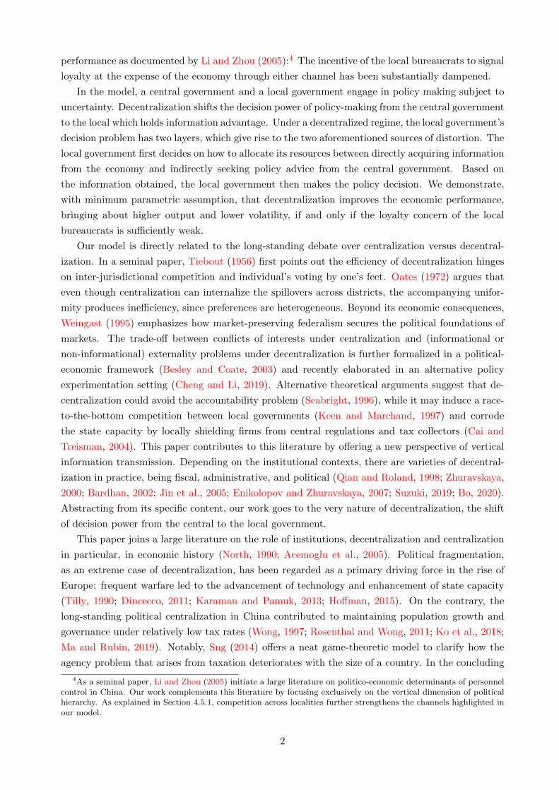
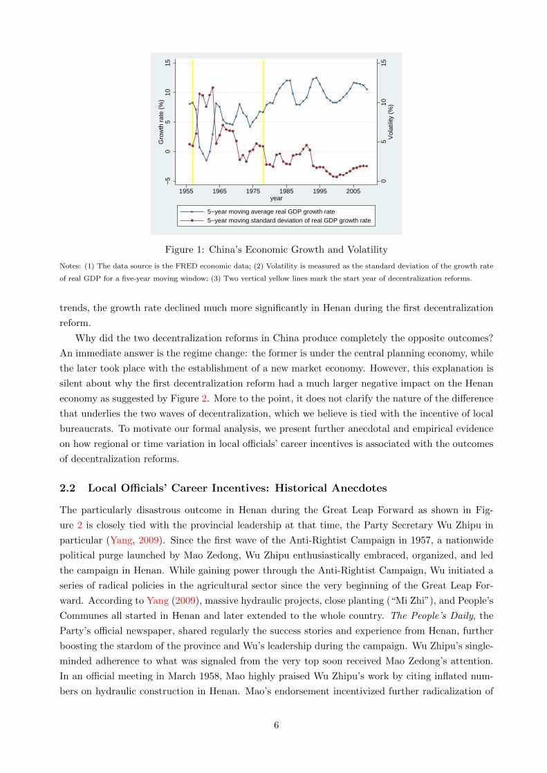
Figure 1 plots China’s GDP growth rate and its output volatility over the past six decades.

Evidently in the figure, economic growth tanked dramatically following the first wave of decentral-

ization, while the economy enjoyed much higher growth in the post 1978 reform era. Less attention

has been paid to the output volatility, but the same, contrasting dynamics followed two waves of

decentralization:12 volatility skyrocketed in the late 1950s and it steadily went down after 1978. Be-

sides contrasting experience between the two reforms, there is also substantial heterogeneity across

regions. Figure 2 plots the evolution of GDP growth rate and output volatility using the data from

Henan and Zhejiang, two provinces in central and southern China respectively. Despite similar

10In his famous speech on the relationship between the central and local governments, Mao Zedong pointed out,“the local should be empowered. This helps us build a strong socialist country. It seems not a good idea to squeezethe power from the local” (“On Ten Major Relationships”, April 25, 1956).

11Due to the disappointing outcome of the first wave of decentralization, there were a sequence of re-centralizationand decentralization reforms, albeit at smaller scales, during 1960s and 70s. For more detailed discussions, see Lin etal. (2006).

12The output volatility is calculated in a very simple manner, but as shown in Wang and Yang (2016), the samepattern persists if we detrend the GDP series using HP filter and control for conventional economic factors thatdetermine volatility such as financial development, openness, inventory management, and monetary policy.

5

05

1015

Vol

atili

ty (

%)

−5

05

1015

Gro

wth

rat

e (%

)

1955 1965 1975 1985 1995 2005year

5−year moving average real GDP growth rate5−year moving standard deviation of real GDP growth rate

Figure 1: China’s Economic Growth and Volatility

Notes: (1) The data source is the FRED economic data; (2) Volatility is measured as the standard deviation of the growth rate

of real GDP for a five-year moving window; (3) Two vertical yellow lines mark the start year of decentralization reforms.

trends, the growth rate declined much more significantly in Henan during the first decentralization

reform.

Why did the two decentralization reforms in China produce completely the opposite outcomes?

An immediate answer is the regime change: the former is under the central planning economy, while

the later took place with the establishment of a new market economy. However, this explanation is

silent about why the first decentralization reform had a much larger negative impact on the Henan

economy as suggested by Figure 2. More to the point, it does not clarify the nature of the difference

that underlies the two waves of decentralization, which we believe is tied with the incentive of local

bureaucrats. To motivate our formal analysis, we present further anecdotal and empirical evidence

on how regional or time variation in local officials’ career incentives is associated with the outcomes

of decentralization reforms.

2.2 Local Officials’ Career Incentives: Historical Anecdotes

The particularly disastrous outcome in Henan during the Great Leap Forward as shown in Fig-

ure 2 is closely tied with the provincial leadership at that time, the Party Secretary Wu Zhipu in

particular (Yang, 2009). Since the first wave of the Anti-Rightist Campaign in 1957, a nationwide

political purge launched by Mao Zedong, Wu Zhipu enthusiastically embraced, organized, and led

the campaign in Henan. While gaining power through the Anti-Rightist Campaign, Wu initiated a

series of radical policies in the agricultural sector since the very beginning of the Great Leap For-

ward. According to Yang (2009), massive hydraulic projects, close planting (“Mi Zhi”), and People’s

Communes all started in Henan and later extended to the whole country. The People’s Daily, the

Party’s official newspaper, shared regularly the success stories and experience from Henan, further

boosting the stardom of the province and Wu’s leadership during the campaign. Wu Zhipu’s single-

minded adherence to what was signaled from the very top soon received Mao Zedong’s attention.

In an official meeting in March 1958, Mao highly praised Wu Zhipu’s work by citing inflated num-

bers on hydraulic construction in Henan. Mao’s endorsement incentivized further radicalization of

6

05

1015

2025

05

1015

2025

−10

010

20−

100

1020

1955 1965 1975 1985 1995 2005

Vol

atili

tyV

olat

ility

Gro

wth

rat

e (%

)G

row

th r

ate

(%)

Henan

Zhejiang

5−year moving average real GDP growth rate5−year moving std. dev. of real GDP growth rate

Year

Figure 2: Economic Growth and Volatility at the Provincial Level

Notes: (1) The data source is China Compendium of Statistics; (2) Volatility is measured as the standard deviation of the growth

rate of real GDP for a five-year moving window; (3) Two vertical yellow lines mark the start year of decentralization reforms.

7

policy-making in Henan. From the summer of 1958, fake reports and misleading statistics became

commonplace, and shortly afterwards, Henan was among the provinces hardest hit by the most

tragic famine in human history.

In contrast to Henan is Zhejiang’s experience. Like many southern provinces, shortly before the

establishment of the PRC, Zhejiang started seeing the arrival of the so-called southbound cadres, the

party cadres sent by the new central government to take over and consolidate the political power.

Soon a power struggle arose between the southbound cadre group and the local guerrilla cadre

group.13 Being backed by the central, the southbound cadre group captured major positions in the

new Zhejiang government while the local guerrilla cadre group were largely marginalized during the

power transition. However, because the local guerrilla cadres had been working in the region for

much longer and thus understood better the local social economy, the new government mainly led

by southbound cadres still had to rely on their political competitors in the actual implementation

of policies. With little political support from the top, the political survival of local guerrilla cadres

hinged on the support from the grassroots. Consequently, the local guerrilla cadre group had much

stronger incentives to act in the interests of the masses especially when they sensed the great damage

a campaign like the Great Leap Forward may bring about to the local economy (Zhang and Liu,

2016). By deviating from the policy guidance from the central, the local guerrilla cadre group helped

mitigate the consequences of the nation-wide policy mistake. Going beyond the Great Leap Forward

episode, Zhang et al. (2013) further provide convincing evidence of how this unique power-sharing

structure in Zhejiang in the wake of the establishment of the PRC causally impacted local private

sector development. The legacy had its influences even during the turbulent period of the Cultural

Revolution and manifested itself in the form of a province known for its booming private sector

during the post 1978 reform era.

The two contrasting historical anecdotes underscore the vital role played by local officials’ ca-

reer incentives in shaping the regional variation in decentralization reform outcomes. In the next

subsection, we provide further empirical evidence to illustrate the structural differences in career

incentives between the two decentralization reforms.

2.3 Local Officials’ Career Incentives: Empirical Evidence

Using the historical data, the existing work suggests that the loyalty concern was one of the culprits

of the tragedy during the Great Leap Forward (Kung and Chen, 2011). On the other hand, it

has been highlighted that economic performance has become an important promotion criterion for

local bureaucrats in the post 1978 reform era (Li and Zhou, 2005), while how important the loyalty

concern remains to be is subject to debate (Jia et al., 2015; Fisman et al., 2020). In this subsection,

we demonstrate that relative to Maoist China, the loyalty concern plays a less important role in

promotion of local bureaucrats in post-reform China.

We follow Jia et al. (2015) to use local officials’ connection with the central politicians as the

measurement of loyalty, defined by whether they worked at the same time in the same branch of

the Party, the government, or the army. We focus on the connection between each provincial Party

secretary and the highest central leaders (Mao Zedong, Deng Xiaoping, Jiang Zemin, and Hu Jintao

13For an excellent and insightful account of this historical episode in Zhejiang, see the book by Zhang and Liu(2016).

8

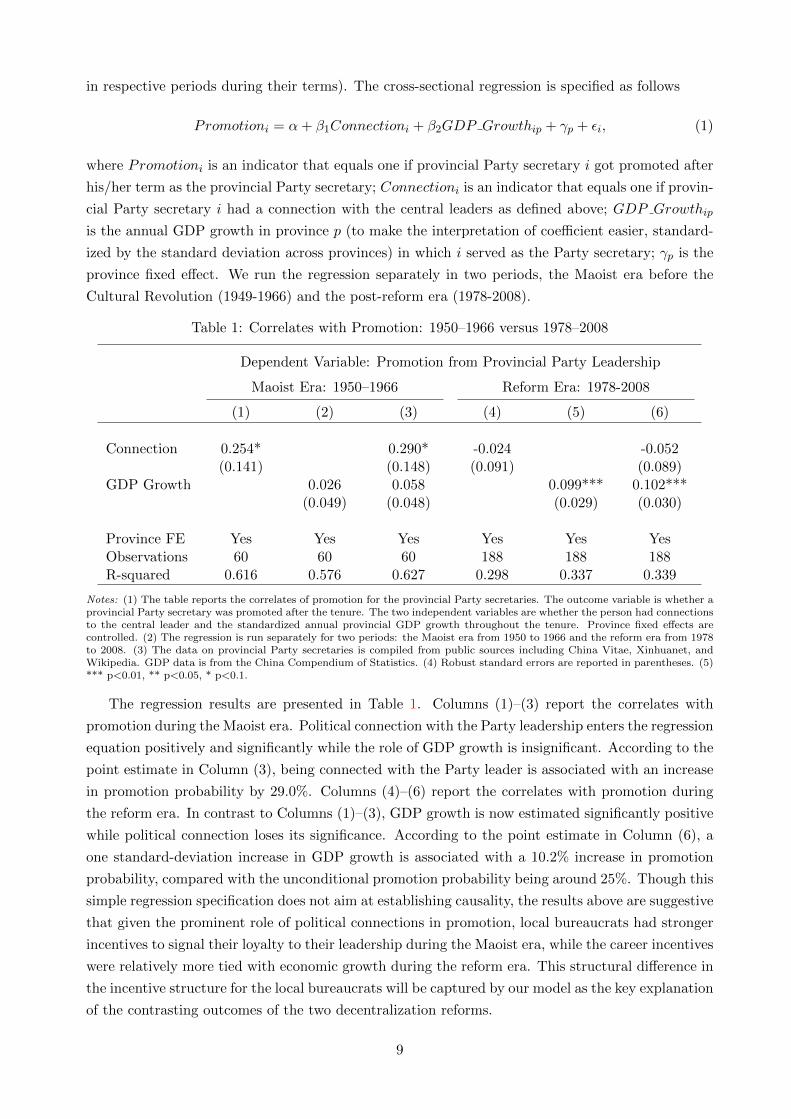
in respective periods during their terms). The cross-sectional regression is specified as follows

Promotioni = α+ β1Connectioni + β2GDP Growthip + γp + εi, (1)

where Promotioni is an indicator that equals one if provincial Party secretary i got promoted after

his/her term as the provincial Party secretary; Connectioni is an indicator that equals one if provin-

cial Party secretary i had a connection with the central leaders as defined above; GDP Growthip

is the annual GDP growth in province p (to make the interpretation of coefficient easier, standard-

ized by the standard deviation across provinces) in which i served as the Party secretary; γp is the

province fixed effect. We run the regression separately in two periods, the Maoist era before the

Cultural Revolution (1949-1966) and the post-reform era (1978-2008).

Table 1: Correlates with Promotion: 1950–1966 versus 1978–2008

Dependent Variable: Promotion from Provincial Party Leadership

Maoist Era: 1950–1966 Reform Era: 1978-2008

(1) (2) (3) (4) (5) (6)

Connection 0.254* 0.290* -0.024 -0.052(0.141) (0.148) (0.091) (0.089)

GDP Growth 0.026 0.058 0.099*** 0.102***(0.049) (0.048) (0.029) (0.030)

Province FE Yes Yes Yes Yes Yes YesObservations 60 60 60 188 188 188R-squared 0.616 0.576 0.627 0.298 0.337 0.339

Notes: (1) The table reports the correlates of promotion for the provincial Party secretaries. The outcome variable is whether aprovincial Party secretary was promoted after the tenure. The two independent variables are whether the person had connectionsto the central leader and the standardized annual provincial GDP growth throughout the tenure. Province fixed effects arecontrolled. (2) The regression is run separately for two periods: the Maoist era from 1950 to 1966 and the reform era from 1978to 2008. (3) The data on provincial Party secretaries is compiled from public sources including China Vitae, Xinhuanet, andWikipedia. GDP data is from the China Compendium of Statistics. (4) Robust standard errors are reported in parentheses. (5)*** p<0.01, ** p<0.05, * p<0.1.

The regression results are presented in Table 1. Columns (1)–(3) report the correlates with

promotion during the Maoist era. Political connection with the Party leadership enters the regression

equation positively and significantly while the role of GDP growth is insignificant. According to the

point estimate in Column (3), being connected with the Party leader is associated with an increase

in promotion probability by 29.0%. Columns (4)–(6) report the correlates with promotion during

the reform era. In contrast to Columns (1)–(3), GDP growth is now estimated significantly positive

while political connection loses its significance. According to the point estimate in Column (6), a

one standard-deviation increase in GDP growth is associated with a 10.2% increase in promotion

probability, compared with the unconditional promotion probability being around 25%. Though this

simple regression specification does not aim at establishing causality, the results above are suggestive

that given the prominent role of political connections in promotion, local bureaucrats had stronger

incentives to signal their loyalty to their leadership during the Maoist era, while the career incentives

were relatively more tied with economic growth during the reform era. This structural difference in

the incentive structure for the local bureaucrats will be captured by our model as the key explanation

of the contrasting outcomes of the two decentralization reforms.

9

2.4 Historical Reforms in Other Countries

Finally, it is worth emphasizing that even though our discussion revolves around the reform his-

tory of China, reforms featuring decentralization of decision making have been taking place across

countries under the authoritarian regime since the late 1980s. Among Asian countries, Viet Nam

launched its large-scale reform (“Doi Moi”) in 1986 which shared many similar characteristics with

the China’s 1978 reform (World Bank, 1993; St John, 1997). In the same year, Laos initiated a

structural reform program called “New Economic Mechanism” (“Chintanakhan Mai”) (Stuart-Fox,

2005). A few years later, Cambodia entered a decade-long process of decentralization reform which

made its breakthrough in early 2000s (Un and Ledgerwood, 2003; World Bank, 2015). In 2001,

known as one of the most radical decentralization reforms, Indonesia started its big bang reform

that packages together economic, political, and administrative decentralizations (Kassum et al.,

2003; Yap, 2018). Unlike Viet Nam, Laos, and Cambodia, Indonesia’s decentralization reform is

accompanied with a prolonged phase of democratization after which the country is no longer under

the authoritarian regime. South Korea, to some extent, follows a similar path despite having a

more dramatic democratization process and a more gradual process of decentralization. All these

reforms share the common ingredient of shifting the economic decision from the central to the local

governments. Like the 1978 reform in China, the impact of those reforms is generally positive, albeit

less conclusive.14

3 The Baseline Model

We model policy making under uncertainty. There are two players, a central government and a

local government. They want to implement an economic policy that hinges on the true state of

the economy subject to uncertainty. There are two channels through which the governments can

reduce the uncertainty. Each government can directly acquire information of the true state of the

economy. It can also acquire information from the other government through the inter-governmental

communication which is nevertheless subject to communication friction. In the baseline setting, the

communication friction is endogenously determined. We will present a version of the model with

exogenous communication friction in the section on extensions, highlighting under what condition

the endogenous communication channel is essential to our main results. Each government has a fixed

amount of resource, which can be allocated between the two activities: direct information acquisition

and indirect information acquisition by reducing the friction in inter-governmental communication.

We consider two economic regimes. Under the centralized regime, the communication is bottom-

up. The local government directly acquires information and then sends a noisy signal to the central

government. Facing the trade-off between the two information acquisition channels, the central gov-

ernment decides how to allocate its attention resource and chooses the economic policy accordingly.

Under the decentralized regime, the communication is top-down. The central government directly

acquires information and sends a noisy signal to the local government. The local government allo-

cates its attention resource and then implements its desired economic policy. Figure 3 illustrates

respectively the timeline of the model under the two regimes.

14We plot how output growth and volatility evolve over the reform period for these four Asian countries in theappendix. See Figures 8 and 9.

10

Figure 3: Timeline

11

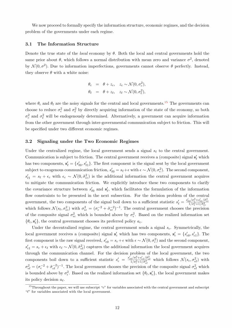
We now proceed to formally specify the information structure, economic regimes, and the decision

problem of the governments under each regime.

3.1 The Information Structure

Denote the true state of the local economy by θ. Both the local and central governments hold the

same prior about θ, which follows a normal distribution with mean zero and variance σ2, denoted

by N (0, σ2). Due to information imperfections, governments cannot observe θ perfectly. Instead,

they observe θ with a white noise:

θc = θ + zc, zc ∼ N (0, σ2c ),

θ` = θ + z`, z` ∼ N (0, σ2` ),

where θc and θ` are the noisy signals for the central and local governments.15 The governments can

choose to reduce σ2c and σ2

` by directly acquiring information of the state of the economy, so both

σ2c and σ2

` will be endogenously determined. Alternatively, a government can acquire information

from the other government through inter-governmental communication subject to friction. This will

be specified under two different economic regimes.

3.2 Signaling under the Two Economic Regimes

Under the centralized regime, the local government sends a signal s` to the central government.

Communication is subject to friction. The central government receives a (composite) signal s′` which

has two components, s′` = {s′`0, s′`1}. The first component is the signal sent by the local government

subject to exogenous communication friction, s′`0 = s`+ε with ε ∼ N (0, σ2ε ). The second component,

s′`1 = s` + εc with εc ∼ N (0, σ2εc) is the additional information the central government acquires

to mitigate the communication friction. We explicitly introduce these two components to clarify

the covariance structure between s′`0 and s′`, which facilitates the formulation of the information

flow constraints to be presented in the next subsection. For the decision problem of the central

government, the two components of the signal boil down to a sufficient statistic s′` =s′`0/σ

2ε+s′`1/σ

2εc

1/σ2ε+1/σ2

εc

which follows N (s`, σ2εc) with σ2

εc = (σ−2ε + σ−2

εc )−1. The central government chooses the precision

of the composite signal σ2εc which is bounded above by σ2

ε . Based on the realized information set

{θc, s′`}, the central government chooses its preferred policy ac.

Under the decentralized regime, the central government sends a signal sc. Symmetrically, the

local government receives a (composite) signal s′c which has two components, s′c = {s′c0, s′c1}. The

first component is the raw signal received, s′c0 = sc+ε with ε ∼ N (0, σ2ε ) and the second component,

s′c1 = sc + ε` with ε` ∼ N (0, σ2ε`) captures the additional information the local government acquires

through the communication channel. For the decision problem of the local government, the two

components boil down to a sufficient statistic s′c =s′c0/σ

2ε+s′c1/σ

2ε`

1/σ2ε+1/σ2

ε`which follows N (sc, σ

2ε`) with

σ2ε` = (σ−2

ε + σ−2ε` )−1. The local government chooses the precision of the composite signal σ2

ε` which

is bounded above by σ2ε . Based on the realized information set {θ`, s′c}, the local government makes

its policy decision a`.

15Throughout the paper, we will use subscript “c” for variables associated with the central government and subscript“`” for variables associated with the local government.

12

The friction in information transmission is pervasive in any large organization, but it could be

particularly severe in the context of an authoritarian government. For the top-down communica-

tion, the friction comes from the lack of transparency of discussions and debates at the very top

and the tendency of over-simplifying real economic issues in policy documents,16 not to mention

the complication of coupling policy prescription with political propaganda.17 For the bottom-up

communication, it is also essential for the central to read between the lines to better understand

the reports from the local. The random or intentional noise accumulates over the long process of

reporting from the very bottom of the regime.

From now on, we assume that s` = θ` and sc = θc. In one of the extensions, we will allow

the signal sender to strategically introduce noise into the inter-governmental communication.18 We

assume all the white noises zc, z`, ε, ε`, and εc are independent.

3.3 The Information Flow Constraint

The decision problem for the government that decides the economic policy, that is, the signal

receiver, has two layers. It has to first decide the resource allocation over two channels of information

acquisition and then choose the optimal policy based on the information gathered.

We first formalize the resource allocation problem. We assume that each government can only

acquire a fixed amount of information following the framework of rational inattention (Sims, 2003;

Mackowiak and Wiederholt, 2009). To formalize the notion of information, we define the differential

entropy as in the standard information theory, which is a measure of the uncertainty of a continuous

random variable.19

Definition 1. The differential entropy H(X) of a continuous random variable X with a probability

density function f(x) is defined as

H(X) = E[− log2 f(x)] = −∫f(x) log2 f(x)dx.

If X follows a multivariate normal distribution with a covariance matrix Σ, it can be shown that

the entropy of X is given by

H(X) =n

2log2(2πe) +

1

2log2 |Σ|,

where n is the dimension of the random variable and |Σ| is the determinant of Σ.

16In an authoritarian regime, the official policy documents are usually the product of the input from the technocrats,fights and compromises among the few decision makers, and politico-economic needs. Wu (1995) presents an excellentstudy of the so-called “Documentary Politics” in China. His case studies detail the whole political process of draftingand disseminating official documents, explaining why even specific wording or quotation could have deep connotations.

17For example, in the May of 1958, the second meeting of the Eighth National Congress of the Party approved thatthe “overall strategy” is to “achieve greater, faster, better, and more economical results in building socialism”. Dueto the political climate in late 1950s, tremendous emphasis was put on quantity and speed with quality and efficiencybeing effectively unnoticed while communicating this overall strategy to the lower level governments, which contributesto the disastrous Great Leap Forward.

18To be sure, misreporting and manipulation are quite common under the authoritarian regime. For the strikingexample of over-reporting, see the announcements of agricultural output during the Great Leap Forward period inChina. In contrast, for fear of the ratchet effect, managers in Soviet Union had great incentive to under-report (Weitz-man, 1976). However, since our main focus is on the tradeoff between different channels of information acquisition inrelation to the resulting policy choice, we abstract from misreporting in this model.

19See, for example, chapter 8 in Cover and Thomas (2012) for a standard treatment.

13

Definition 2. The conditional differential entropy H(X|Y ) of two continuous random variables X

and Y with a joint probability density function f(x, y) is defined as

H(X|Y ) = −∫f(x, y) log2 f(x|y)dxdy.

In general, we have

H(X|Y ) = H(X,Y )−H(Y ).

Hence, if one is interested in X, the informativeness of an observation Y can be captured by the

difference between H(X)−H(X|Y ). In other words, the difference between H(X) and H(X|Y ) is

the reduction of uncertainty with respect to X when Y is observed. In the framework of rational

inattention, we assume that each economic agent has limited attention resource, so its information

flow constraint is generally given by H(X)−H(X|Y ) < κ. We now specialize this constraint to our

setting.

Under the centralized regime, the information flow constraint for the signal sender, the local

government, is given by

H(θ)−H(θ|θ`) ≤ κ` ⇔1

2log2

(Var(θ)

Var(θ|θ`)

)=

1

2log2

(σ2 + σ2

`

σ2`

)≤ κ`, (2)

where κ` > 0 is the capacity of information acquisition of the local government.

For the central government, the reduction of entropy comes from two sources: improved infor-

mation about both θ and ε. The constraint on the entropy reduction is then given by

H(θ, ε|s′`0)−H(θ, ε|θc, s′`) ≤ κc,

where κc > 0 is the capacity of information acquisition of the central government.

Notice that even though θ and ε are unconditionally independent, we cannot write the con-

straint in an additively separable form for θ and ε as they might not be independent conditional

on the acquired information (θc, s′`).

20 The following lemma provides a closed form solution to this

information flow constraint.21

Lemma 1. The information flow constraint of the central government under the centralized regime

is given by (1

σ2`

+1

σ2εc

)(1

σ2+

1

σ2`

+1

σ2c

)≤

22κc(σ2 + σ2` + σ2

ε )

σ2σ2`σ

2ε

+1

σ4`

≡ Kc(σ2` ). (3)

Equation 3 may appear a bit complicated, but the choice variables, σ2c and σ2

εc for the central

government are multiplicatively separable, which is very important for a sharp characterization of

the attention allocation problem. Moreover, we have K` ≥(1/σ2

ε + 1/σ2`

) (1/σ2 + 1/σ2

`

)with the

equality if and only if κc = 0, i.e., if the central government has zero information capacity, then it

is impossible to acquire any information (σ2εc = σ2

ε and σ2c = ∞). It should be noted that σ2

` , the

signal precision of the local government, enters the above constraint. In what follows, we sometimes

20This stands in sharp contrast with the earlier macroeconomic applications of rational inattention such as Mack-owiak and Wiederholt (2009). Conditional correlation substantially complicates the analytics of the model.

21All the proofs are relegated to the appendix.

14

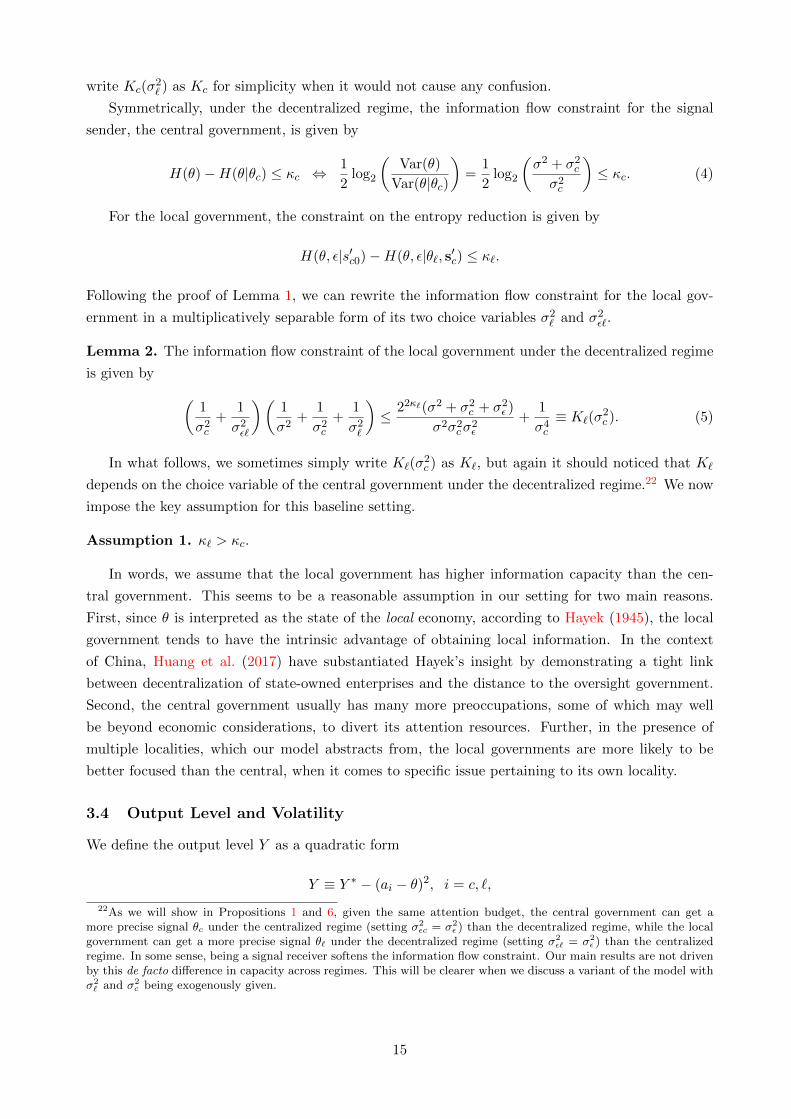
write Kc(σ2` ) as Kc for simplicity when it would not cause any confusion.

Symmetrically, under the decentralized regime, the information flow constraint for the signal

sender, the central government, is given by

H(θ)−H(θ|θc) ≤ κc ⇔1

2log2

(Var(θ)

Var(θ|θc)

)=

1

2log2

(σ2 + σ2

c

σ2c

)≤ κc. (4)

For the local government, the constraint on the entropy reduction is given by

H(θ, ε|s′c0)−H(θ, ε|θ`, s′c) ≤ κ`.

Following the proof of Lemma 1, we can rewrite the information flow constraint for the local gov-

ernment in a multiplicatively separable form of its two choice variables σ2` and σ2

ε`.

Lemma 2. The information flow constraint of the local government under the decentralized regime

is given by (1

σ2c

+1

σ2ε`

)(1

σ2+

1

σ2c

+1

σ2`

)≤ 22κ`(σ2 + σ2

c + σ2ε )

σ2σ2cσ

2ε

+1

σ4c

≡ K`(σ2c ). (5)

In what follows, we sometimes simply write K`(σ2c ) as K`, but again it should noticed that K`

depends on the choice variable of the central government under the decentralized regime.22 We now

impose the key assumption for this baseline setting.

Assumption 1. κ` > κc.

In words, we assume that the local government has higher information capacity than the cen-

tral government. This seems to be a reasonable assumption in our setting for two main reasons.

First, since θ is interpreted as the state of the local economy, according to Hayek (1945), the local

government tends to have the intrinsic advantage of obtaining local information. In the context

of China, Huang et al. (2017) have substantiated Hayek’s insight by demonstrating a tight link

between decentralization of state-owned enterprises and the distance to the oversight government.

Second, the central government usually has many more preoccupations, some of which may well

be beyond economic considerations, to divert its attention resources. Further, in the presence of

multiple localities, which our model abstracts from, the local governments are more likely to be

better focused than the central, when it comes to specific issue pertaining to its own locality.

3.4 Output Level and Volatility

We define the output level Y as a quadratic form

Y ≡ Y ∗ − (ai − θ)2, i = c, `,

22As we will show in Propositions 1 and 6, given the same attention budget, the central government can get amore precise signal θc under the centralized regime (setting σ2

εc = σ2ε ) than the decentralized regime, while the local

government can get a more precise signal θ` under the decentralized regime (setting σ2ε` = σ2

ε ) than the centralizedregime. In some sense, being a signal receiver softens the information flow constraint. Our main results are not drivenby this de facto difference in capacity across regimes. This will be clearer when we discuss a variant of the model withσ2` and σ2

c being exogenously given.

15

where Y ∗ is the ideal output level if the policy choice ac or a` perfectly matches the true state of

the economy θ. In this paper, we are particularly interested in the ex ante expected output level

E(Y ) and its variance V ar(Y ).

3.5 The Decision Problem for Each Government

Under the decentralized regime, the central government, which is the signal sender, is assumed to

be benevolent. Its decision problem is given by

maxσ2c

E(Y ) = Y ∗ − E(a` − θ)2,

subject to Constraint 4.

The local government, which receives the signal from the central, has a two-layer decision prob-

lem, which is given by

maxσ2` ,σ

2ε`

E

{maxa`

(1− γ)(Y ∗ − E[(a` − θ)2|θ`, s′c]

)− γE[(a` − θc)2|θ`, s′c]

},

subject to Constraint 5 and σ2ε` ≤ σ2

ε . Suggested by the objective function, beyond economic output,

the local government is also concerned with whether its economic policy follows closely enough the

signal sent by the central. The local government has the incentive to stick to the policy prescription

of the central, signaling its political loyalty. This additional career concern seems to be a common

characteristics in many authoritarian regimes,23 and it turns out to be the key driving force of our

main results.

The parameter γ ∈ [0, 1] captures the importance of signaling political loyalty relative to eco-

nomic consideration in policy making. From now on we simply interpret γ as loyalty concern but

our comparative static results should be understood as a change of either political or economic

incentives. When γ = 0, the objective of the local government is perfectly aligned with that of the

central government. When γ = 1, the local government attaches no importance to economic output

and only attempts to induce the central government to adopt its policy recommendation. During

the reform in the late 1950s, under a more coercive system with greater emphasis on political loyalty,

the central government faces a high γ. In the 1978 reform, the change of political climate, as well as

more focus placed on economic development, yields a lower γ. It should be noted that γ reflects the

institutional constraints faced by the central government and thus is not a choice variable at least

in the short run and as far as economic policy-making is concerned.

An important asymmetry arises in the objective function between the local and central gov-

ernment. For simplicity, the central government is assumed to be benevolent. This assumption

presumes that the central government can separate political consideration from economic motiva-

tion while the local government cannot. Alternatively, we could assume that the central government

indeed cares about conformity of the local as well, but as long as its loyalty concern is not as strong

23Besides the Great Leap Forward in China, Nikita Khrushchev’s Corn Campaign is another infamous example.Seeing the increase of corn production as an important part of his agricultural reform, Khrushchev initiated a largescale expansion program of corn production in mid 1950s. With his strong backing, the area of corn cultivation grewexponentially, which was later proven to be quite unproductive and inefficient. However, according to a detailed casestudy by Hale-Dorrell (2014), even subordinates had recognized the absurdity of the corn campaign much earlier,deception, submission, and fine-tuning were widespread.

16

as the local’s in the domain of economic policy decisions, the intuition of our main results would

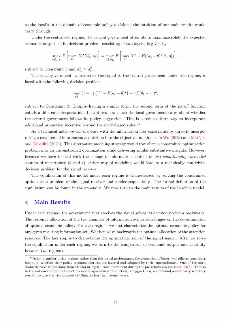
carry through.

Under the centralized regime, the central government attempts to maximize solely the expected

economic output, so its decision problem, consisting of two layers, is given by

maxσ2c ,σ

2εc

E

[maxac

E(Y |θc, s′`)]

= maxσ2c ,σ

2εc

E

[maxac

Y ∗ − E((ac − θ)2|θc, s′`)],

subject to Constraint 3 and σ2εc ≤ σ2

ε .

The local government, which sends the signal to the central government under this regime, is

faced with the following decision problem

maxσ2`

(1− γ)(Y ∗ − E(ac − θ)2

)− γE(θ` − ac)2,

subject to Constraint 2. Despite having a similar form, the second term of the payoff function

entails a different interpretation. It captures how much the local government cares about whether

the central government follows its policy suggestion. This is a reduced-form way to incorporate

additional promotion incentive beyond the merit-based rules.24

As a technical note, we can dispense with the information flow constraints by directly incorpo-

rating a cost item of information acquisition into the objective function as in Wu (2019) and Matejka

and Tabellini (2020). This alternative modeling strategy would transform a constrained optimization

problem into an unconstrained optimization while delivering similar substantive insights. However,

because we have to deal with the change in information content of two conditionally correlated

sources of uncertainty (θ and ε), either way of modeling would lead to a technically non-trivial

decision problem for the signal receiver.

The equilibrium of this model under each regime is characterized by solving the constrained

optimization problem of the signal receiver and sender sequentially. The formal definition of the

equilibrium can be found in the appendix. We now turn to the main results of the baseline model.

4 Main Results

Under each regime, the government that receives the signal solves its decision problem backwards.

The resource allocation of the two channels of information acquisition hinges on the determination

of optimal economic policy. For each regime, we first characterize the optimal economic policy for

any given resulting information set. We then solve backwards the optimal allocation of the attention

resource. The last step is to characterize the optimal decision of the signal sender. After we solve

the equilibrium under each regime, we turn to the comparison of economic output and volatility

between two regimes.

24Under an authoritarian regime, rather than the actual performance, the promotion of lower-level officers sometimeshinges on whether their policy recommendations are favored and adopted by their superordinates. One of the mostdramatic cases is “learning-from-Dazhai-in-Agriculture” movement during the pre-reform era (Meisner, 1978). Thanksto the nation-wide promotion of his model agricultural production, Yonggui Chen, a community-level party secretaryrose to become the vice premier of China in less than twenty years.

17

4.1 Optimal Economic Policy

Because of the quadratic objective function, the optimal policy of the final policy maker is a linear

combination of the signals it receives. Under the centralized regime, the benevolent central govern-

ment always targets its policy to the expected state of the economy conditional on all the signals

it gathers. For the closed-form solution to the central government’s policy, see Lemma 12 in the

appendix. We can write the distance between the policy and the true state of the economy as

E(ac − θ)2 = V ar(θ|θc, s′`) =

(1

σ2+

1

σ2c

+1

σ2` + σ2

εc

)−1

. (6)

which suggests that direct information acquisition has a first-order impact on reducing the expected

deviation through σ2c , while the contribution of inter-governmental communication through σ2

εc is

constrained by the quality of the signal sent by the local, σ2` .

Under the decentralized regime, the local government’s policy choice, formally stated as Lemma

13 in the appendix, is a weighted average of the optimal policy chosen by the local government if

it were benevolent (the case of γ = 0) and the local government’s conditional expectation of the

signal from the central (the case of γ = 1). The loyalty concern of the local government introduces

distortion directly through the policy-making margin. In the absence of loyalty concern (γ = 0),

the distance between the chosen policy and the true state of the economy is symmetric to what we

have obtained under the centralized regime:

E(a` − θ)2∣∣∣γ=0

= V ar(θ|θ`, s′c) =

(1

σ2+

1

σ2`

+1

σ2c + σ2

ε`

)−1

(7)

On the other hand, when the local government is entirely loyalty driven (γ = 1), the distance

between the policy and its best guess of the central government’s signal is of the similar form of

harmonic mean:

E(a` − θc)2∣∣∣γ=1

= V ar(θc|θ`, s′c) =

(1

σ2ε`

+1

σ2c + (1/σ2 + 1/σ2

` )−1

)−1

, (8)

which implies that, to minimize the distance between a` and θc, inter-governmental communication

tends to be more effective than direct information acquisition.

Since the optimal policy chosen by the signal receiver is always a linear combination of all the

signals it obtains, we obtain a tight relationship between the expected output and output volatility.

Lemma 3. Let ai be a linear combination of all the signals: θ`, θc, s′`, and s′c (i = c, `). The

expected output is given by

E(Y ) ≡ Y ∗ − E(ai − θ)2 and V ar(Y ) = 2(Y ∗ − E(Y ))2.

The lemma shows that the output level and volatility move in the opposite direction, and as a

result, the comparative statics concerning the output level can easily be re-interpreted in terms of

volatility. From now on, we will mainly work with E(Y ), or more directly, the deviation of policy

from the true state of the economy, E(ai − θ)2.

18

4.2 The Equilibrium under the Centralized Regime

Under the centralized regime, there is a sharp characterization of the equilibrium. First, the central

government spends all of its attention budget on direct information acquisition.25 Since the central

government cares only about economic output and direct information acquisition has a first-order

impact on economic output, the central has no incentive to divert its resource to inter-governmental

communication. As a result, σ2εc = σ2

ε . Second, the local government also devotes itself to direct

information acquisition.26 On the one hand, the economic motive (the term (1 − γ)EY in the

objective function) incentivizes the local government to increase the precision of the signal it sends

to the central. On the other hand, since the central government attaches more importance to the

signal sent by the local government if the quality of the signal is higher, the political motive (the

term −γE(ac − θ`)2) gives additional incentive for the local government to maximize its effort to

acquire information. Since all the attention budget of the local is spent on information acquisition,

Constraint 2 is binding, leading to σ2` = σ2/(22κ` −1). The following proposition formally states the

equilibrium characterization under the centralized regime.

Proposition 1. Under the centralized regime, we have

E(ac − θ)2 =

(1

σ2+

1

σ2c

+1

σ2` + σ2

ε

)−1

with σ2` = σ2/(22κ` − 1), σ2

εc = σ2ε , and

σ2c =

[Kc

(1

σ2ε

+1

σ2`

)−1

− 1

σ2− 1

σ2`

]−1

=σ2(σ2

ε + σ2` )

(22κc − 1)(σ2 + σ2ε + σ2

` ).

4.3 The Equilibrium under the Decentralized Regime

The equilibrium characterization under the decentralized regime is more involved, which hinges on

the degree of loyalty concern γ. To proceed, we first provide the following characterization of how

the local government allocates its attention budget for any given γ.

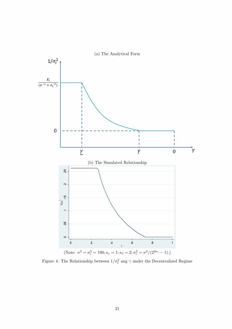
Lemma 4. Under the decentralized regime, there exist two cutoffs γ and γ such that 0 < γ < γ < 1.

If γ ≤ γ, the local government specializes in direct information acquisition (σ2ε` = σ2

ε ). If γ ≥ γ, the

local government specializes in intergovernmental communication (σ2` =∞). If γ ∈ (γ, γ), the local

government allocates its budget to both activities (σ2` <∞ and σ2

ε` < σ2ε ) with

1

σ2`

+1

σ2+

1

σ2c

=K

1/2` (1− γ)

γ, (9)

which implies that ∂σ2` /∂γ > 0.

According to this lemma,27 the parameter space of γ can be partitioned into three subsets. The

local government focuses exclusively on intergovernmental communication if its loyalty concern is

25See Lemma 14 in the appendix.26See Lemma 15 in the appendix.27As a technical note, we prove this lemma by first showing that the information flow constraint must be binding.

Using the binding constraint, we recast the decision problem as an unconstrained univariate optimization problem.We then solve the optimization problem for γ in different ranges. Moreover, γ and γ can be solved in closed form.

19

sufficiently strong (γ ≥ γ). Intuitively, if the main concern of the local bureaucrats is to infer the

signal sent by the central government, then they can best achieve this goal by directly reducing the

inter-governmental communication friction, at the cost of not acquiring any additional information

about the true state of the economy.28 Second, the local government focuses exclusively on direct

information acquisition provided that the economic motive is sufficiently strong (γ ≤ γ). This case

is symmetric to the equilibrium under the centralized regime. Last, if the loyalty concern is in the

intermediate range, then the attention resource will be allocated to both channels with the effort

on intergovernmental communication strictly increasing with the intensity of the loyalty concern.

We illustrate the relationship between 1/σ2` with γ in Figure 4. Clearly, the precision of the

signal acquired by the local government (weakly) decreases with γ. The loyalty concern could

heavily influence the information acquisition margin of the local government. On top of the policy-

making margin, this is the second margin that the loyalty concern distorts the economy, which turns

out to be indispensable for generating differential economic outcomes under decentralization.

We turn to the strategy of the central government under the decentralized regime. A better

signal from the central helps the local target the true state of the economy, but it is also possible

that a better signal induces the local to spend more effort on inter-governmental communication,

leading to a waste of the attention budget from the standpoint of social welfare. In our frame-

work, the first channel dominates, so the central government always maximizes its effort to direct

information acquisition. The actual proof is tedious because the strategy of the local government is

not differentiable with respect to γ at the two cutoffs and the two cutoffs γ and γ themselves are

functions of σ2c .

Lemma 5. Under the decentralized regime, for any γ, the central government spends all of its

attention resource on information acquisition (Constraint 4 is binding), which leads to

σ2c = σ2/(22κc − 1).

Given the sharp characterization of the strategy of the central government, we can establish the

counterpart of Proposition 1 under the decentralized regime.29 More importantly, we establish the

following monotonicity result that is crucial for the comparison of economic performance between

the two regimes.

Proposition 2. Under the decentralized regime, E(a` − θ)2 strictly increases with γ.

In words, the stronger the loyalty concern is, the further away the economic policy is from the

true state of the local economy.

They are roots in [0, 1] to the following two equations respectively:

γ2 − (1− γ)2K−1` (1/σ2

ε + 1/σ2c )2 = 0

γ2 − (1− γ)2K`(1/σ2 + 1/σ2

c )−2 = 0.

28It is noted that the local government could also infer the central government’s signal by acquiring informationabout θ, but it is indirect and turns out to be less efficient.

29See Propositions 6 and 7 for two special cases in the appendix.

20

(a) The Analytical Form

(b) The Simulated Relationship

(Note: σ2 = σ2ε = 100;κc = 1;κ` = 2;σ2

c = σ2/(22κc − 1).)

Figure 4: The Relationship between 1/σ2` ang γ under the Decentralized Regime

21

4.4 Comparison between Two Regimes

In the absence of loyalty concern, governments under each regime focus exclusively on direct infor-

mation acquisition. The intergovernmental communication friction has an asymmetric impact on

information transmission under the two regimes. Under the centralized regime, it is the better signal

received by the central that becomes noisier, while under the decentralized regime, it is the worse

signal received by the local that becomes noisier. To predict the true state of the economy, one high

quality signal is better than two mediocre quality signals. Therefore, if γ = 0, the decentralized

regime performs better (higher expected output and lower volatility). The assumption that the local

government has higher information capacity (Assumption 1) is essential to this result.30

Lemma 6. E(ac − θ)2 > E(a` − θ)2∣∣∣γ=0

.

On the other hand, decentralization with γ = 1 always worsens economic performance. Distor-

tion in the information acquisition margin leads to strictly less informative signals for the decision

maker, the local government. The economic outcome further deteriorates due to distortion in the

policy making margin.

Lemma 7. E(ac − θ)2 < E(a` − θ)2∣∣∣γ=1

.

Following Proposition 2 and Lemmas 3, 6, and 7, we now obtain the core result of the paper.

Theorem 1. There exists a unique γ in (0, 1) such that E(ac − θ)2 = E(a` − θ)2∣∣∣γ=γ

. If γ >

γ, decentralization worsens economic performance; if γ < γ, decentralization improves economic

performance.

This result highlights the pivotal role played by the loyalty concern in determining the economic

outcome of decentralization in an authoritarian regime. Despite the information advantage held by

the local, decentralization could be detrimental to the economy if the local bureaucrats have strong

incentive to follow the policy suggestions from the central. Figure 5 illustrates the comparison

between two economic regimes in relation to the degree of loyalty concern γ. Notice there are two

kinks on the curve of E(a`−θ)2 at which γ = γ or γ. The curve is much steeper in the middle range

as both margins of loyalty-driven distortion are effectively at work.

Corollary 1. γ > γ.

The corollary suggests that for decentralization to be welfare-improving, we should expect local

bureaucrats to at least spend some effort on direct information acquisition.31 In light of the intuition

behind Lemma 7, the devotion of local bureaucrats to understanding and deciphering the policy

message from the top guarantees the failure of decentralization.

4.5 Discussion

4.5.1 Revisiting China’s Reform History

In light of our theory, the difference in γ could help explain the contrasting experience following the

two decentralization reforms in China and possibly the heterogeneous outcomes across regions. In

30As made clear in the proof, for γ = 0, decentralization improves economic performance if and only if κ` > κc.31On the other hand, there is no clear relationship between γ and γ. Consider two numerical example. First, we

let σ2 = σ2ε = 100, κ` = 2κc = 2. We find that γ ≈ 0.27 and γ ≈ 0.47. Then, we reduce σ2

ε to be 10, which leads toγ ≈ 0.33 and γ ≈ 0.26.

22

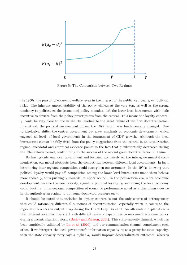
Figure 5: The Comparison between Two Regimes

the 1950s, the pursuit of economic welfare, even in the interest of the public, can bear great political

risks. The inherent unpredictability of the policy choices at the very top, as well as the strong

tendency to politicalize the (economic) policy mistakes, left the lower-level bureaucrats with little

incentive to deviate from the policy prescriptions from the central. This means the loyalty concern,

γ, could be very close to one in the 50s, leading to the great failure of the first decentralization.

In contrast, the political environment during the 1978 reform was fundamentally changed. Due

to ideological shifts, the central government put great emphasis on economic development, which

engaged all levels of local governments in the tournament of GDP growth. Although the local

bureaucrats cannot be fully freed from the policy suggestions from the central in an authoritarian

regime, anecdotal and empirical evidence points to the fact that γ substantially decreased during

the 1978 reform period, contributing to the success of the second great decentralization in China.

By having only one local government and focusing exclusively on the inter-governmental com-

munication, our model abstracts from the competition between different local governments. In fact,

introducing inter-regional competition could strengthen our argument. In the 1950s, knowing that

political loyalty would pay off, competition among the lower level bureaucrats made them behave

more radically, thus pushing γ towards its upper bound. In the post-reform era, since economic

development became the new priority, signaling political loyalty by sacrificing the local economy

could backfire. Inter-regional competition of economic performance acted as a disciplinary device

in the authoritarian regime to put some downward pressure on γ.

It should be noted that variation in loyalty concern is not the only source of heterogeneity

that could rationalize differential outcomes of decentralization, especially when it comes to the

regional differences in output drop during the Great Leap Forward. An alternative explanation is

that different localities may start with different levels of capabilities to implement economic policy

during a decentralization reform (Besley and Persson, 2014). This state-capacity channel, which has

been empirically validated by Lu et al. (2020), and our communication channel complement each

other. If we interpret the local government’s information capacity κ` as a proxy for state capacity,

then the state capacity story says a higher κ` would improve decentralization outcomes, whereas

23

our analysis enriches this argument by including a qualification: decentralization is only welfare

improving when the loyalty concern is not too strong; otherwise building the local government’s

information capacity would be in vain.

4.5.2 Reinterpreting the Model in the Context of Democracies

Throughout our modeling exercise, we focus exclusively on a hierarchical authoritarian regime, but

our formulation and results can also be reinterpreted in the context of democracies, thus shedding

light on the role of voters’ information-processing capacity in representative democracies.32 To rein-

terpret the model, we relabel the central government as voters and the local government as the

elected politicians. The centralized regime in our model can be viewed as classical Athenian democ-

racies, in which voters directly deliberate and decide on policy-making while the politicians’ role is

to help voters make informed decisions. The decentralized regime can be viewed as representative

democracies, in which it is the elected politicians who enact legislation. Our Theorem 1 suggests

that, representative democracies tend to produce better outcomes than classical democracies, which

is consistent with the fact that modern democracies are predominantly representative democracies;

however, perhaps more importantly, in the presence of communication frictions and information

processing constraints, when voters possess less precise information, larger inefficiencies may arise

from representative democracies (for example, in the form of populist parties) when the politicians

have very strong incentives to pander to voters. Policy-making mostly driven by voter opinion

erodes the informational advantage of the representative democracies.

Closely related to this reinterpretation is the recent work by Matejka and Tabellini (2020). In

their model, they consider an electoral competition between two opportunistic politicians for ra-

tionally inattentive voters. Due to the interplay between endogenous information acquisition and

opportunistic policy making, greater availability of information may have negative welfare conse-

quences. Albeit in different settings, both models point to the critical importance of information

processing constraints in understanding the distortions in political processes. More broadly, the rein-

terpretation connects our model to a larger literature examining electoral accountability through

the lens of contractual theory. As reviewed by Ashworth (2012), a key insight from this literature is

that politicians’ incentive to “impress the voters” may be conflicted with “the normative imperative

to advance the voter’s interests”. There is a direct parallelism between this tension in the models

of political agency and the loyalty concern in our formulation.

5 Extensions

To check the robustness of our model prediction, we consider three extensions. The first extension

shuts down the channel of endogenous information transmission between governments. In this non-

strategic environment, if the exogenous communication friction is large enough, then decentralization

always benefits the economy. Thus, the inter-governmental communication channel is essential to

generating differential outcomes of decentralization. Moreover, in this simplified setting, a seemingly

paradoxical relationship arises: the economic performance improves with the noisiness of the inter-

32We gratefully acknowledge one of our referees for his/her suggestion and advice to write this subsection. It isto bring out an insightful reinterpretation and an intriguing connection elucidated in the referee report between ourmodel and the issues arising from informational asymmetry in a democratic environment.

24

governmental communication friction, as higher exogenous communication friction incentivizes the

local government to focus on its self-obtained and more precise information in the policy marking.

This finding echoes the earlier result due to Board et al. (2007) in a cheap-talk environment. The

second extension introduces strategic communication and the third extension relaxes the assumption

of information advantage of the local. We discuss how the main insights of this paper adapt to those

extensions.

5.1 Exogenous Communication Frictions

The first extension shuts down the endogenous communication channel. It concerns whether the

model will deliver our main results when loyalty concern only operates through the final decision-

making margin and, under what condition, the endogenous communication channel is essential to

generating differential outcomes of decentralization.

The basic setup is very similar. The main departure is that σ2` and σ2

c are exogenously given.

In particular, we assume that each government receives a private signal about θ from the nature.

The private signal of the central government θc follows N (θ, σ2c ), while the private signal of the local

government θ` follows ∼ N (θ, σ2` ) with σ2

` and σ2c exogenously given. We assume σ2

c > σ2` , that is,

the local government receives a more precise signal than the central government. The quality of the

signal (σ2` or σ2

c ) is the same under both regimes.

Under the centralized regime, the local government sends its signal s` = θ` to the central. The

central government receives a signal s′` with s′` = s` + ε. Upon receiving the signal, the central

government makes the policy choice ac based on the private information θc and the signal received

s′`. Similarly, under the decentralized regime, the central government sends a signal sc = θc. The

local government receives a signal s′c with s′c = sc + ε. The local government then picks its preferred

policy a` based on θ` and s′c. We assume ε ∼ N (0, σ2ε ) with σ2

ε being exogenous. The model

otherwise follows the baseline setting. Figure 6 illustrates the timeline of the model without rational

inattention.

Abstracting from the strategic behavior in this simplified framework, the decision problem of

the signal receiver is only to determine the desired economic policy.

Under the centralized regime, the decision problem of the central government is given by

maxac

E(Y |θc, s′`) = Y ∗ − E[(ac − θ)2|θc, s′`],

Under the decentralized regime, the decision problem of the local government is given by

maxa`

(1− γ)(Y ∗ − E[(a` − θ)2|θ`, s′c]

)− γE[(a` − sc)2|θ`, s′c].

Solving for the optimal policy, we again find that the government policy is always a linear

combination of two private signals, θc and θ`, and the communication friction ε.33 According to

Lemma 3, to analyze economic output and volatility, we only need to focus on E(ac − θ)2 and

E(a` − θ)2.34

33See Lemma 18 in the appendix.34For the explicit expressions of E(ac − θ)2 and E(a` − θ)2 under γ = 0 and γ = 1, see Lemma 19 in the appendix.

25

Figure 6: Timeline without Rational Inattention

26

Lemma 8. In the absence of the loyalty concern (γ = 0), decentralization improves the economic

performance.

Following the same intuition as in the benchmark model, the assumption σ2` < σ2

c and the

presence of communication friction play a crucial role in the above result. However, the outcome of

decentralization under γ = 1 is now less clear.

Lemma 9. Under the decentralized regime with γ = 1, there exists a unique σ2ε > 0 such that

E(a` − θ)2 = E(ac − θ)2 for σ2ε = σ2

ε and E(a` − θ)2 > E(ac − θ)2 if and only if σ2ε < σ2

ε .

To understand this result, consider two thought experiments. If the communication friction

vanishes, this non-strategic environment coincides with the benchmark model and therefore, our

earlier results carry over. The local government ignores its self-obtained and more precise signal

and simply follow the policy prescription from the central government, thus leading to a worse

economic outcome. To the other extreme, if the communication is prohibitively noisy (σ2ε → ∞),

the local government cannot rely on the signal it receives from the central government to predict

sc. Instead, it has to rely on its own signal, which is correlated with the original signal sent by the

central, sc, via the mutual component θ. In this case, decentralization could be welfare improving

even in the presence of pure loyalty concern.

This result stands in sharp contrast with Lemma 7 in which decentralization under γ = 1 always

leads to worse economic performance. The difference precisely stems from the missing endogenous

communication margin.

It can be easily seen from Lemma 19 that the expected output strictly decreases with σ2ε under

the centralized regime and the decentralized regime with γ = 0. When governments attempt to

maximize the expected output, additional communication friction worsens the economic outcome.

However, the intuition gets reversed when we turn to a purely loyalty-driven local government. In

fact, we can prove the following seemingly paradoxical result: higher communication friction could

be welfare improving under decentralization.

Proposition 3. Under the decentralized regime with γ = 1, ∂E(a` − θ)2/∂(σ2ε ) < 0.

This result underscores the insights behind the two thought experiments conducted above.

Higher communication friction, on the one hand, makes information transmission more difficult,

but on the other hand, makes the local government effectively more independent from the central

in policy-making. The second channel dominates when γ = 1.

We now prove a counterpart of Proposition 2 in this alternative setup. In the absence of strategic

considerations, the proof turns out to be much simpler.

Corollary 2. Under the decentralized regime in a non-strategic environment, E(a` − θ)2 strictly

increases with γ.

Now we are ready to provide the main theorem in this non-strategic environment, a complete

characterization of the relative economic performance under two regimes.

Theorem 2. In a non-strategic environment, there exists a unique σ2ε > 0 such that

1. if σ2ε > σ2

ε , decentralization always improves economic performance

27

2. if σ2ε < σ2

ε , there exists a unique γ ∈ (0, 1) such that (i) if γ < γ, decentralization improves

economic performance; (ii) if γ > γ, decentralization worsens economic performance.

The differential outcomes of decentralization emerge only when the exogenous communication

friction is sufficiently small. When inter-governmental communication is sufficiently noisy, this non-

strategic environment predicts that decentralization is always welfare improving, even for γ = 1. This

is because distortion in the information acquisition margin is muted and thus loyalty concern only

impacts the policy making margin. When there is substantial exogenous communication friction,

distortion in the policy making margin is not large enough to alter the sign of the outcome under

decentralization.

5.2 Strategic Communication

In the baseline setting, we assume that the signal sender always reveals its information truthfully:

s` = θ` under the centralized regime and sc = θc under the decentralized regime. We now relax this

assumption by allowing the signal sender to introduce additional noise to its signal. In particular,

under the decentralized regime, we assume the local government sends a signal of the form

s` = θ` + δ`

with δ` ∼ N (0, σ2δ`). Under the decentralized regime, the central government sends a signal of the

form

sc = θc + δc

with δc ∼ N (0, σ2δc). We assume that the signal sender can choose any σ2

δ` (or σ2δc) costlessly.

The local government’s decision problem can be modeled in two different ways.35 First, if the

local government attempts to target its policy to the central government’s original signal θc, then

the objective function is given by

maxσ2` ,σ

2ε`

E

{maxa`

(1− γ)(Y ∗ − E[(a` − θ)2|θ`, s′c]

)− γE[(a` − θc)2|θ`, s′c]

}.

In this case, the local government’s information acquisition decision hinges on σ2δc, which is summa-

rized by the following proposition.

Proposition 4. Under the decentralized regime with γ = 1, there exist two cutoffs for σ2δc: σ

2δc and

σ2δc. If σ2

δc ≥ σ2δc, then σ2

ε` = σ2ε ; If σ2

δc ≤ σ2δc, σ

2` =∞; if σ2

δc ∈ (σ2δc, σ

2δc), then σ2

` strictly decreases

with σ2δc.

The proposition suggests a (weakly) monotonically decreasing relationship between σ2` and σ2

δc.

For a large σ2δc, the return of acquiring information about the central government’s private signal

θc through communication is lower and thus the local government has stronger incentives for direct

information acquisition. As a result, strategic communication gives rise to a new type of equilib-

rium: knowing that the local government may divert their attention resources to recover the central

35We are indebted to one of the referees for the rewriting of this subsection. The second case is incorporated inlight of his/her insightful comment.

28

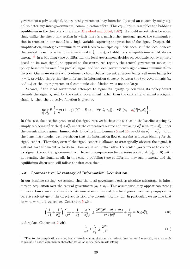
government’s private signal, the central government may intentionally send an extremely noisy sig-

nal to deter any inter-governmental communication effort. This equilibrium resembles the babbling

equilibrium in the cheap-talk literature (Crawford and Sobel, 1982). It should nevertheless be noted

that, unlike the cheap-talk setting in which there is a much richer message space, the communica-

tion instrument in our model is a single variable capturing the precision of the signal. Despite this

simplification, strategic communication still leads to multiple equilibria because if the local believes

the central to send a non-informative signal (σ2δc = ∞), a babbling-type equilibrium would always

emerge.36 In a babbling-type equilibrium, the local government decides on economic policy entirely

based on its own signal, as opposed to the centralized regime, the central government makes its

policy based on its own (less precise) signal and the local government’s signal-cum-communication-

friction. Our main results will continue to hold, that is, decentralization being welfare-reducing for

γ = 1, provided that either the difference in information capacity between the two governments (κ`

and κc) or the inter-governmental communication friction σ2ε is not too large.

Second, if the local government attempts to signal its loyalty by orienting its policy target

towards the signal sc sent by the central government rather than the central government’s original

signal θc, then the objective function is given by

maxσ2` ,σ

2ε`

E

{maxa`

(1− γ)(Y ∗ − E[(a` − θ)2|θ`, s′c]

)− γE[(a` − sc)2|θ`, s′c]

}.

In this case, the decision problem of the signal receiver is the same as that in the baseline setting by

simply replacing σ2` with σ2

` +σ2δ` under the centralized regime and replacing σ2

c with σ2c +σ2

δc under

the decentralized regime. Immediately following from Lemmas 5 and 15, we obtain σ2δ` = σ2

δc = 0. In

the benchmark model, we have shown that the information flow constraint is always binding for the

signal sender. Therefore, even if the signal sender is allowed to strategically obscure the signal, it

will not have the incentive to do so. However, if we further allow the central government to conceal

its signal, the central government will have to compare sending a noiseless signal (σ2δc = 0) with

not sending the signal at all. In this case, a babbling-type equilibrium may again emerge and the

equilibrium discussion will follow the first case then.

5.3 Comparative Advantage of Information Acquisition

In our baseline setting, we assume that the local government enjoys absolute advantage in infor-

mation acquisition over the central government (κ` > κc). This assumption may appear too strong

under certain economic situations. We now assume, instead, the local government only enjoys com-

parative advantage in the direct acquisition of economic information. In particular, we assume that

κ` = κc = κ, and we replace Constraint 5 with(1

σ2c

+1

σ2ε`

)(1

σ2+

1

σ2c

+λ

σ2`

)≤ 22κ(σ2 + σ2

c + σ2ε )

σ2σ2cσ

2ε

+1

σ4c

≡ K`(σ2c ), (10)

and replace Constraint 2 with1

σ2+

λ

σ2`

≤ 22κ

σ2, (11)

36Due to the complication arising from strategic communication in a rational inattention framework, we are unableto provide a sharp equilibrium characterization as in the benchmark setting.

29

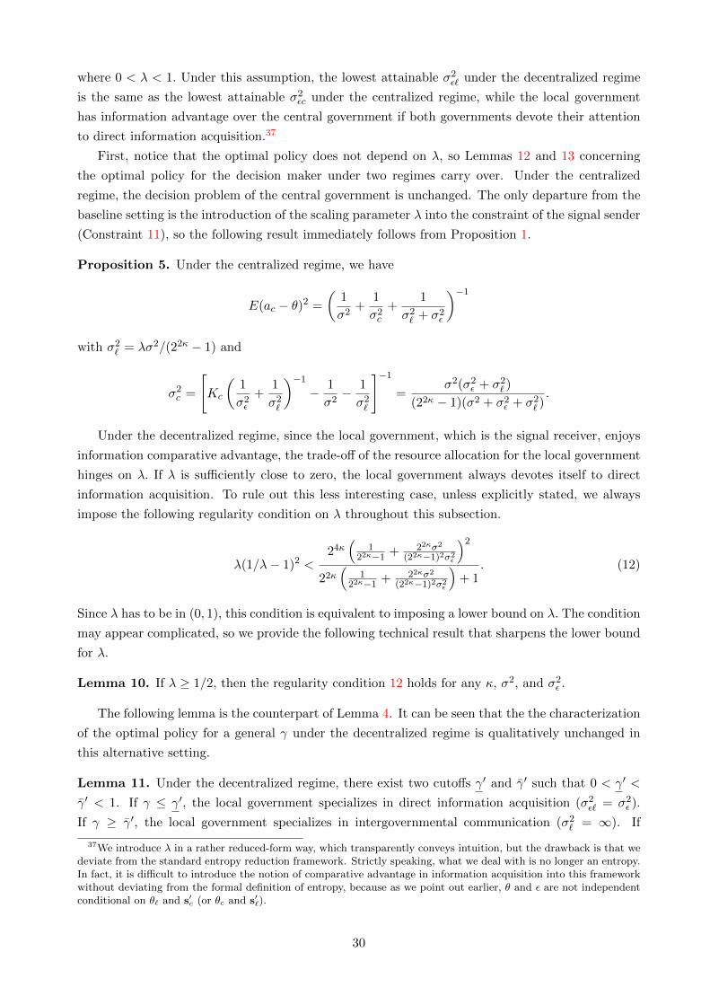
where 0 < λ < 1. Under this assumption, the lowest attainable σ2ε` under the decentralized regime

is the same as the lowest attainable σ2εc under the centralized regime, while the local government

has information advantage over the central government if both governments devote their attention

to direct information acquisition.37

First, notice that the optimal policy does not depend on λ, so Lemmas 12 and 13 concerning

the optimal policy for the decision maker under two regimes carry over. Under the centralized

regime, the decision problem of the central government is unchanged. The only departure from the

baseline setting is the introduction of the scaling parameter λ into the constraint of the signal sender

(Constraint 11), so the following result immediately follows from Proposition 1.

Proposition 5. Under the centralized regime, we have

E(ac − θ)2 =

(1

σ2+

1

σ2c

+1

σ2` + σ2

ε

)−1

with σ2` = λσ2/(22κ − 1) and

σ2c =

[Kc

(1

σ2ε

+1

σ2`

)−1

− 1

σ2− 1

σ2`

]−1

=σ2(σ2

ε + σ2` )

(22κ − 1)(σ2 + σ2ε + σ2

` ).

Under the decentralized regime, since the local government, which is the signal receiver, enjoys

information comparative advantage, the trade-off of the resource allocation for the local government

hinges on λ. If λ is sufficiently close to zero, the local government always devotes itself to direct

information acquisition. To rule out this less interesting case, unless explicitly stated, we always

impose the following regularity condition on λ throughout this subsection.

λ(1/λ− 1)2 <24κ(

122κ−1

+ 22κσ2

(22κ−1)2σ2ε

)2

22κ(

122κ−1

+ 22κσ2

(22κ−1)2σ2ε

)+ 1

. (12)

Since λ has to be in (0, 1), this condition is equivalent to imposing a lower bound on λ. The condition

may appear complicated, so we provide the following technical result that sharpens the lower bound

for λ.

Lemma 10. If λ ≥ 1/2, then the regularity condition 12 holds for any κ, σ2, and σ2ε .

The following lemma is the counterpart of Lemma 4. It can be seen that the the characterization

of the optimal policy for a general γ under the decentralized regime is qualitatively unchanged in

this alternative setting.

Lemma 11. Under the decentralized regime, there exist two cutoffs γ′ and γ′ such that 0 < γ′ <

γ′ < 1. If γ ≤ γ′, the local government specializes in direct information acquisition (σ2ε` = σ2

ε ).

If γ ≥ γ′, the local government specializes in intergovernmental communication (σ2` = ∞). If

37We introduce λ in a rather reduced-form way, which transparently conveys intuition, but the drawback is that wedeviate from the standard entropy reduction framework. Strictly speaking, what we deal with is no longer an entropy.In fact, it is difficult to introduce the notion of comparative advantage in information acquisition into this frameworkwithout deviating from the formal definition of entropy, because as we point out earlier, θ and ε are not independentconditional on θ` and s′c (or θc and s′`).

30

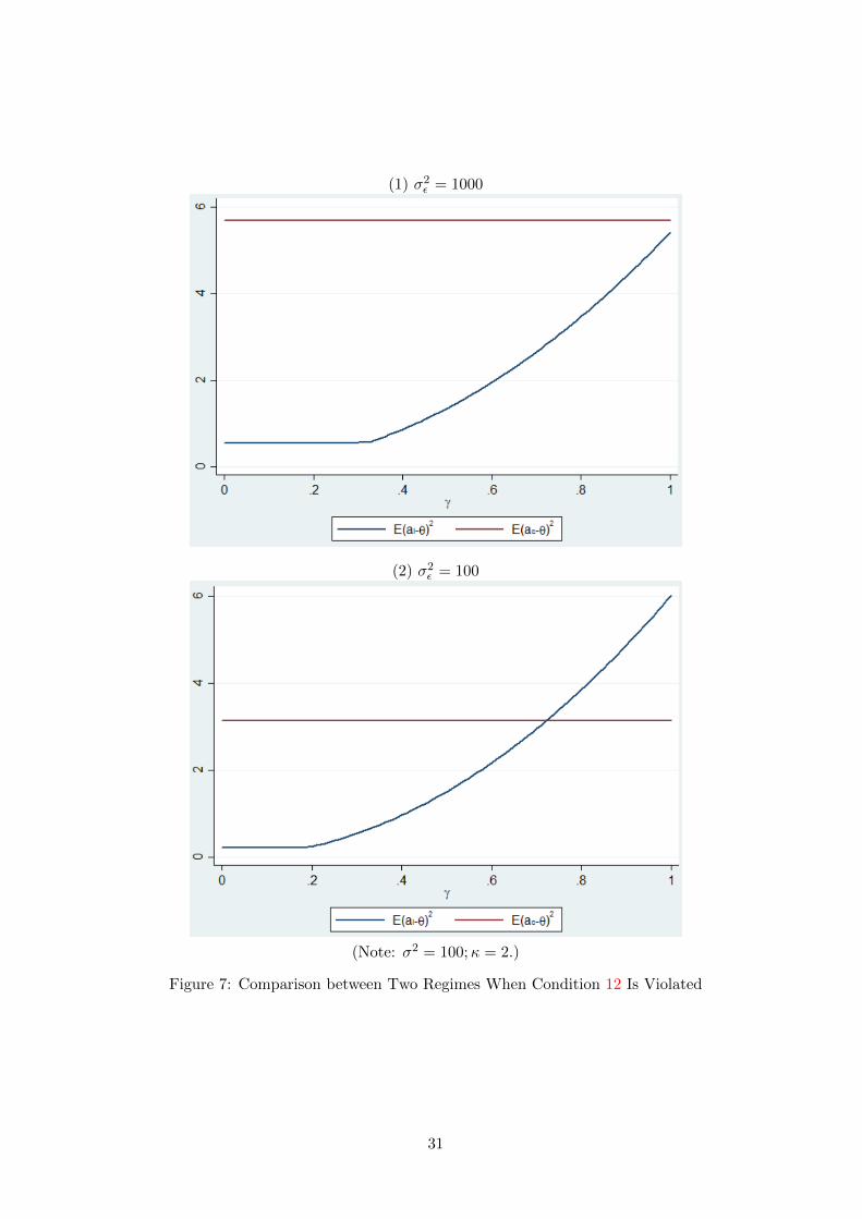
(1) σ2ε = 1000

(2) σ2ε = 100

(Note: σ2 = 100;κ = 2.)

Figure 7: Comparison between Two Regimes When Condition 12 Is Violated

31

γ ∈ (γ′, γ′), the local government allocates its budget to both activities (σ2` <∞ and σ2

ε` < σ2ε ) with

∂σ2` /∂γ > 0.

However, due to the complication for γ in the middle range, it is very challenging to establish

the counterpart of Theorem 1 in this setting. Instead, we provide a slightly weaker result which

nevertheless captures the main insight.

Theorem 3. If γ is sufficiently close to one, decentralization worsens economic performance; if γ

is sufficiently close to zero, decentralization improves economic performance.

Albeit not being formally established, our simulation results suggest that the comparison between

two regimes seems very similar to what has been illustrated by Figure 5: economic volatility increases

monotonically with γ and there are two kinks on the curve of E(a`−θ)2, representing the structural

changes of the local government’s optimal strategy when γ = γ′ and γ = γ′.

To close this subsection, we consider the case the local government has very strong comparative

advantage such that Condition 12 does not hold. In this case, γ′ disappears. Since there is no equi-

librium characterization for the middle range of γ, we perform a battery of numerical experiments.

As shown in Figure 7, other things equal, when σ2ε is relatively large, then decentralization always

leads to improvement of economic performance; when σ2ε is relatively small, then the economic out-

come of decentralization hinges on γ. The numerical results are qualitatively similar to what we

have shown for the setting with exogenous communication friction.

6 Conclusion

In this paper, we propose a model of inter-governmental information transmission to understand the

political economy of decentralization. The model demonstrates that the impact of decentralization

on economic performance hinges on the degree of loyalty concern of the local government. Decen-

tralization leads to higher volatility and lower output, if the local government is a loyal follower

of the central government. A closer examination of the underlying mechanism reveals that loyalty

concern impacts the economic outcome of decentralization through two margins: policy making

and information acquisition. The latter turns out to be crucial for welfare-reducing decentralization

to emerge from our theoretical construction. The main result sheds light the sub-context of our

model, the contrasting dynamics following the two waves of decentralization in China. It highlights

the complex interplay between loyalty concern, inter-governmental communication, and friction

therein. Therefore, for policy makers, evaluation of the past decentralization reforms requires a

better understanding of political distortion deeply embedded in the system.

Our work can be extended in several directions. Empirically, it would be interesting to directly

test the model prediction by applying text analysis of official government documents. Does a

loyalty-driven local government tend to spend more time in inter-governmental communication?

Is there a general trend of how lower level governments study and interpret directives from their

superordinates from the Maoist era to the reform era? Theoretically, the model can be extended

to accommodate multiple local governments. Once competition across localities is put into play,

under what condition will information distortion through inter-governmental communication be

further amplified? More importantly, if we allow the local governments to be heterogeneous in their

information capacity, could we further incorporate the insights from the state capacity literature

32

into our model? Moreover, given its generality, our analytical framework can be reframed to help

understand decentralization experience in other authoritarian countries and more broadly, large

organizations with internal hierarchies. We leave all these avenues for future research.

33

A Proofs and Some Unreported Results

A.1 Proof of Lemma 1

Proof. Since H(θ, ε|s′`0) = H(θ, ε, s′`0) − H(s′`0) and H(θ, ε|θc, s′`) = H(θ, ε, θc, s′`) − H(θc, s

′`), we

have38

H(θ, ε|s′`0)−H(θ, ε|θc, s′`) = H(θ, ε, s′`0) +H(θc, s′`)−H(s′`0)−H(θ, ε, θc, s

′`)

=1

2

(log2 |Σθ,ε,s′`0

|+ log2 |Σθc,s′`| − log2 |Σs′`0

| − log2 |Σθ,ε,θc,s′`|)≤ κc.

Under the assumption of the model, we have |Σs′`0| = σ2 + σ2

` + σ2ε and

|Σθ,ε,s′`0| =

∣∣∣∣∣∣∣σ2 0 σ2

0 σ2ε σ2

ε

σ2 σ2ε σ2 + σ2

` + σ2ε

∣∣∣∣∣∣∣ = σ2σ2εσ

2` ,

|Σθc,s′`| =

∣∣∣∣∣∣∣σ2 + σ2

c σ2 σ2

σ2 σ2 + σ2` + σ2

ε σ2 + σ2`

σ2 σ2 + σ2` σ2 + σ2

` + σ2εc

∣∣∣∣∣∣∣ = (σ2 +σ2c )(σ

2` σ

2εc+σ

2ε σ

2εc+σ

2εσ

2` )+σ2

cσ2(σ2

εc+σ2ε ),

|Σθ,ε,θc,s′`| =

∣∣∣∣∣∣∣∣∣∣∣∣

σ2 0 σ2 σ2 σ2

0 σ2ε 0 σ2

ε 0

σ2 0 σ2 + σ2c σ2 σ2

σ2 σ2ε σ2 σ2 + σ2

` + σ2ε σ2 + σ2

`

σ2 0 σ2 σ2 + σ2` σ2 + σ2

` + σ2εc

∣∣∣∣∣∣∣∣∣∣∣∣= σ2σ2

εσ2cσ

2` σ

2εc.

Plugging the terms into the information flow constraint, we obtain(1

σ2cσ

2ε

+1

σ2σ2ε

+1

σ2cσ

2`

+1

σ2σ2`

+1

σ2c σ

2εc

+1

σ2σ2εc

+1

σ2εσ

2`

+1

σ2` σ

2εc

)≤ 22κc

σ2 + σ2` + σ2

ε

σ2σ2εσ

2`

.

Using σ2εc = (σ−2

ε + σ−2εc )−1 and simplifying the equation, we obtain the desired conclusion.

A.2 Proof of Lemma 2

Proof. Since H(θ, ε|s′c0) = H(θ, ε, s′c0)−H(s′c0) and H(θ, ε|θ`, s′c) = H(θ, ε, θ`, s′c)−H(θ`, s

′c),

H(θ, ε|s′c0)−H(θ, ε|θ`, s′c) = H(θ, ε, s′c0) +H(θ`, s′c)−H(s′c0)−H(θ, ε, θ`, s

′c)

=1

2

(log2 |Σθ,ε,s′c0

|+ log2 |Σθ`,s′c | − log2 |Σs′c0| − log2 |Σθ,ε,θ`,s′c |

)≤ κ`.

Under the assumption of the model, we have |Σs′c0| = σ2 + σ2

c + σ2ε and

|Σθ,ε,s′c0| =

∣∣∣∣∣∣∣σ2 0 σ2

0 σ2ε σ2

ε

σ2 σ2ε σ2 + σ2

c + σ2ε

∣∣∣∣∣∣∣ = σ2σ2εσ

2c ,

38Alternatively, for two multivariate normal distributions X and Y , we have |ΣX|Y ||ΣY | = |ΣX |.

34

|Σθ`,s′c | =

∣∣∣∣∣∣∣σ2 + σ2

` σ2 σ2

σ2 σ2 + σ2c + σ2

ε σ2 + σ2c

σ2 σ2 + σ2c σ2 + σ2

c + σ2ε`

∣∣∣∣∣∣∣ = (σ2 +σ2` )(σ

2c σ

2ε`+σ

2ε σ

2ε`+σ

2εσ

2c )+σ2

`σ2(σ2

ε`+σ2ε ),

|Σθ,ε,θ`,s′c | =

∣∣∣∣∣∣∣∣∣∣∣∣

σ2 0 σ2 σ2 σ2

0 σ2ε 0 σ2

ε 0

σ2 0 σ2 + σ2` σ2 σ2

σ2 σ2ε σ2 σ2 + σ2

c + σ2ε σ2 + σ2

c

σ2 0 σ2 σ2 + σ2c σ2 + σ2

c + σ2ε`

∣∣∣∣∣∣∣∣∣∣∣∣= σ2σ2

εσ2cσ

2` σ

2ε`.

Plugging the terms into the information flow constraint, we obtain(1

σ2ε

+1

σ2ε`

+1

σ2c

)(1

σ2+

1

σ2`

)+

1

σ2c

(1

σ2ε`

+1

σ2ε

)+

1

σ4c

≤ 22κ`σ2 + σ2

c + σ2ε

σ2σ2εσ

2c

+1

σ4c

.

Using σ2ε` = (σ−2

ε + σ−2ε` )−1 and simplifying the equation, we obtain the desired conclusion.

A.3 Equilibrium Definition

We now formally define the (perfect Bayesian Nash) equilibrium of the sequential game under each

regime. In both regimes, we require the belief updating follows the Bayes’ rule.39 The equilibrium

under the centralized regime is defined as a quadruplet (σ∗`2, σ∗c

2(·), σ∗εc2(·), a∗c(·)) such that for any

quintuplet (σ2` , σ

2c , σ

2εc; θc, s

′`),

a∗c(σ2` , σ

2c , σ

2εc; θc, s

′`) ∈ arg max

acE(Y ∗ − (ac − θ)2|θc, s′`);

For any σ2` > 0,

(σ∗c2(σ2

` ), σ∗εc

2(σ2` )) ∈ arg max

σ2c ,σ

2εc

E(Y ∗ − (a∗c(σ2` , σ

2c , σ

2εc; θc, s

′`)− θ)2)

subject to Constraint 3 and σεc2 ≤ σ2

ε ;

σ∗`2 ∈ arg max

σ2`

{(1− γ)(Y ∗ − E(a∗c(σ

2` , σ∗c

2(σ2` ), σ

∗εc

2(σ2` ); θc, s

′`)− θ)2)

−γE(θ` − a∗c(σ2` , σ∗c

2(σ2` ), σ

∗εc

2(σ2` ); θc, s

′`))

2}

subject to Constraint 2.

The equilibrium under the decentralized regime is defined as a quadruplet (σ∗c2, σ∗`

2(·), σ∗ε`2(·), a∗` (·))

such that for any quintuplet (σ2c , σ

2` , σ

2ε`; θ`, s

′c),

a∗` (σ2c , σ

2` , σ

2ε`; θ`, s

′c) ∈ arg max

a`(1− γ)E(Y ∗ − (a` − θ)2|θ`, s′c)− γE[(a` − θc)2|θ`, s′c];

For any σ2c > 0,

(σ∗`2(σ2

c ), σ∗ε`

2(σ2c )) ∈ arg max

σ2` ,σ

2ε`

{(1− γ)E(Y ∗ − (a∗` (σ

2c , σ

2` , σ

2ε`; θ`, s

′c)− θ)2)

39For simplicity, we omit the prior of θ whenever we state the information set.

35

−γE(a∗` (σ2c , σ

2` , σ

2ε`; θ`, s

′c)− θc)2

}subject to Constraint 5 and σε`

2 ≤ σ2ε ;

σ∗c2 ∈ arg max

σ2c

(Y ∗ − E(a∗` (σ2c , σ∗`

2(σ2c ), σ

∗ε`

2(σ2c ); θ`, s

′c)− θ)2)

subject to Constraint 4.

A.4 The Optimal Policy under the Two Regimes

Lemma 12. Under the centralized regime, the optimal policy of the central government is given by

ac = E(θ|θc, s′`) =

θcσ2c

+s′`

σ2`+σ2

εc

1σ2 + 1

σ2c

+ 1σ2`+σ2

εc

.

Proof. Under the centralized regime, given the quadratic form of the objective function, the optimal

policy for the central government is given by

ac = E(θ|θc, s′`).

To find the expression of the conditional expectation above, we first notice the probability density

function of the joint distribution of (θ, θc, θ`, s′`) can be written as

f(θ, θc, θ`, s′`) = f(θ)f(θc, θ`, s

′`|θ) = f(θ)f(θc|θ)f(θ`, s

′`|θ)

= f(θ)f(θc|θ)f(θ`|θ)f(s′`|θ`) = f(θ)f(θc|θ)f(θ`|θ)f(s′`0|θ`)f(s′`1|θ`),

where the second to last equation stems from the fact that conditional on θ`, ε and εc are independent

of θ. More explicitly, we have40

f(θ, θc, θ`, s′`) ∼ exp

{−1

2

[θ2

σ2+

(θc − θ)2

σ2c

+(θ` − θ)2

σ2`

+(s′`0 − θ`)2

σ2ε

+(s′`1 − θ`)2

σ2εc

]}= exp

{−1

2

[(1

σ2`

+1

σ2ε

+1

σ2εc

)θ2` − 2

(θ

σ2`

+s′`0σ2ε

+s′`1σ2εc

)θ`

+θ2

σ2+

(θc − θ)2

σ2c

+θ2

σ2`

+s′`0

2

σ2ε

+s′`1

2

σ2εc

]}40Alternatively, we know f(θ, θc, θ`, s

′`) ∼ exp

(− 1

2(θ, θc, θ`, s

′`)Σ−1θ,θc,θ`,s

′`(θ, θc, θ`, s

′`)T)

with

Σ−1θ,θc,θ`,s

′`

=

σ2 σ2 σ2 σ2 σ2

σ2 σ2 + σ2c σ2 σ2 σ2

σ2 σ2 σ2 + σ2` σ2 + σ2

` σ2 + σ2`

σ2 σ2 σ2 + σ2` σ2 + σ2

` + σ2ε σ2 + σ2

`

σ2 σ2 σ2 + σ2` σ2 + σ2

` σ2 + σ2` + σ2

εc

−1

=

1σ2 + 1

σ2c

+ 1σ2`− 1σ2c

− 1σ2`

0 0

− 1σ2c

1σ2c

0 0 0

− 1σ2`

0 1σ2`

+ 1σ2ε

+ 1σ2εc− 1σ2ε− 1σ2εc

0 0 − 1σ2ε

1σ2ε

0

0 0 − 1σ2εc

0 1σ2εc

.

36

= exp

−1

2

( 1

σ2`

+1

σ2ε

+1

σ2εc

)θ` − θσ2`

+s′`0σ2ε

+s′`1σ2εc

1σ2`

+ 1σ2ε

+ 1σ2εc

2

+θ2

σ2+

(θc − θ)2

σ2c

+θ2

σ2`

+s′`0

2

σ2ε

+s′`1

2

σ2εc

−

(θσ2`

+s′`0σ2ε

+s′`1σ2εc

)2

1σ2`

+ 1σ2ε

+ 1σ2εc

Integrating out θ` and using s′` =s′`0/σ

2ε+s′`1/σ

2εc

1/σ2ε+1/σ2

εcand σ2

εc = (σ−2ε + σ−2

εc )−1, we obtain

f(θ, θc, s′`) ∼ exp

{−1

2

[(1

σ2+

1

σ2c

+1

σ2` + σ2

εc

)θ2 − 2

(θcσ2c

+s′`

σ2` + σ2

εc

)θ

]}.

This leads to

f(θ|θc, s′`) ∼ f(θ, θc, s′`) ∼ exp

−1

2

(1

σ2+

1

σ2c

+1

σ2` + σ2

εc

)θ − θcσ2c

+s′`

σ2`+σ2

εc

1σ2 + 1

σ2c

+ 1σ2`+σ2

εc

2 ,

which yields the closed-form solution to E(θ|θc, s′`).

Lemma 13. Under the decentralized regime, the optimal policy of the local government is given

by

a` = (1− γ)E(θ|θ`, s′c) + γE(θc|θ`, s′c) = (1− γ)

θ`σ2`

+ s′cσ2c+σ2

ε`

1σ2 + 1

σ2`

+ 1σ2c+σ2

ε`

+ γ

θ`σ2c+σ2

`+σ2cσ

2` /σ

2 + s′cσ2ε`

1σ2c+(1/σ2+1/σ2

` )−1 + 1σ2ε`

.

Proof. Under the decentralized regime, given the quadratic form of the objective function, the

optimal policy for the local government is given by

a` = (1− γ)E(θ|θ`, s′c) + γE(θc|θ`, s′c).

E(θ|θ`, s′c) can be obtained similarly as E(θ|θc, s′`). For E(θc|θ`, s′c), we have

f(θ, θc, θ`, s′c) = f(θ)f(θc|θ)f(θ`|θ)f(s′c0|θc)f(s′c1|θc)

∼ exp

{−1

2

[θ2

σ2+

(θc − θ)2

σ2c

+(θ` − θ)2

σ2`

+(s′c0 − θc)2

σ2ε

+(s′c1 − θc)2

σ2ε`

]}= exp

{−1

2

[(1

σ2+

1

σ2c

+1

σ2`

)θ2 − 2

(θcσ2c

+θ`σ2`

)θ +

θ2c

σ2c

+θ2`

σ2`

+(s′c0 − θc)2

σ2ε

+(s′c1 − θc)2

σ2ε`

]}

= exp

−1

2

( 1

σ2+

1

σ2c

+1

σ2`

)θ − θcσ2c

+ θ`σ2`

1σ2 + 1

σ2c

+ 1σ2`

2

+θ2c

σ2c

+θ2`

σ2`

+(s′c0 − θc)2

σ2ε

+(s′c1 − θc)2

σ2ε`

−

(θcσ2c

+ θ`σ2`

)2

1σ2 + 1

σ2c

+ 1σ2`

.

37

Integrating out θ, we obtain

f(θc, θ`, s′c) ∼ exp

{−1

2

[θ2c

σ2c

+θ2`

σ2`

+(s′c0 − θc)2

σ2ε

+(s′c1 − θc)2

σ2ε`

−(θc/σ

2c + θ`/σ

2` )

2

1/σ2 + 1/σ2c + 1/σ2

`

]}.

Using s′c =s′c0/σ

2ε+s′c1/σ

2ε`

1/σ2ε+1/σ2

ε`and σ2

ε` = (σ−2ε + σ−2

ε` )−1, we obtain

f(θc|θ`, s′c) ∼ f(θc, θ`, s′c) ∼ exp

−1

2

1

σ2ε`

+1

σ2c + 1

1/σ2+1/σ2`

θc − s′cσ2ε`

+ θ`σ2c+σ2

`+σ2cσ

2` /σ

2

1σ2ε`

+ 1σ2c+(1/σ2+1/σ2

` )−1

2 ,

which implies the closed form solution to E(θc|θ`, s′c). Plugging the expressions of E(θ|θ`, s′c) and

E(θc|θ`, s′c) into the equation for a`, we obtain the desired conclusion.

A.5 Proof of Lemma 3

Proof. Since ai is a linear combination of all the signals θ`, θc, s′`, and s′c, we can write (ai − θ) as

a linear combination of six independent normal random variables with mean zero,

ai − θ = mi1(θ` − θ) +mi2(θc − θ) +mi3ε+mi4εc +mi5ε` + (mi1 +mi2 − 1)θ.

Then according to the central moments of a normal distribution, we have

E(ai − θ)2 = m2i1σ

2` +m2

i2σ2c +m2

i3σ2ε +m2

i4σ2εc +m2

i5σ2ε` + (1−mi1 −mi2)2σ2,

E(ai−θ)4 = 3(m2i1σ

2` +m2

i2σ2c +m2

i3σ2ε +m2

i4σ2εc +m2

i5σ2ε` + (1−mi1 −mi2)2σ2

)2= 3

(E(ai − θ)2

)2.

Therefore, by definition,

E(Y ) ≡ Y ∗−E(ai−θ)2 = Y ∗−(m2i1σ

2` +m2

i2σ2c +m2

i3σ2ε +m2

i4σ2εc +m2

i5σ2ε` + (1−mi1 −mi2)2σ2)

),

V ar(Y ) = E(ai − θ)4 −(E(ai − θ)2

)2= 2

(E(ai − θ)2

)2= 2(Y ∗ − E(Y ))2.

A.6 The Equilibrium under the Centralized Regime

According to Lemma 12 and Equation 6, the resource allocation problem for the central government

can be simplified to

maxσ2c ,σ

2εc

1

σ2+

1

σ2c

+1

σ2` + σ2

εc

,

subject to Constraint 3 and σ2εc ≤ σ2

ε . By inspection, the constraint has to be binding. Given the

binding constraint, we can further simplify the constrained optimization problem to

maxσ2c ,σ

2εc

(1− 1

σ4`Kc

)(1

σ2+

1

σ2`

+1

σ2c

)subject to Constraint 3. Since Kc > 1/σ4

` , the maximum is attained when σ2c attains its minimum

under the constraint, or equivalently, σ2εc = σ2

ε . Therefore, we obtain the following characterization

38

of the central government’s strategy under the centralized regime.

Lemma 14. Under the centralized regime, for any given σ2` , the central government completely

devotes itself to the direct information acquisition with σ2εc = σ2

ε .

Our next lemma suggests that the career concern of the local bureaucrats does not distort the

economic outcome under the centralized regime, as long as the central government is benevolent.

Lemma 15. Under the centralized regime, for any γ, the local government always spends all of its

attention resource on information acquisition (Constraint 2 is binding), which leads to

σ2` = σ2/(22κ` − 1).

Proof. According to Lemma 14, under the centralized regime, σ2εc = σ2

ε , so we can simplify ac as

ac =

θcσ2c

+s′`

σ2`+σ2

ε

1σ2 + 1

σ2c

+ 1σ2`+σ2

ε

,

Using the backward induction, the local government solves its decision problem

maxσ2`

(1− γ)(Y ∗ − E(ac − θ)2

)− γE(θ` − ac)2,

or equivalently,

minσ2`

(1− γ)E(ac − θ)2 + γE(θ` − ac)2 ≡ F (σ2` ),

subject to Constraint 2. Plugging in the expression of ac, we can write the objective function

explicitly as

F (σ2` ) = (1− γ)E(ac − θ)2 + γE(θ` − ac)2

= E(ac − θ)2 + 2γE(θ` − θ)(θ − ac) + γE(θ` − θ)2

=1

1σ2 + 1

σ2c

+ 1σ2`+σ2

ε

−2γσ2

`

σ2`+σ2

ε

1σ2 + 1

σ2c

+ 1σ2`+σ2

ε

+ γσ2`

Since we know σ2εc = σ2

ε , Constraint 3 gives us(1

σ2ε

+1

σ2`

)(1

σ2+

1

σ2`

+1

σ2c

)= Kc(σ

2` ) = 22κc

σ2 + σ2` + σ2

ε

σ2σ2`σ

2ε

+1

σ4`

.

The difficulty of this optimization problem can be seen from the equation above. Despite the fact

that the central government always devotes to direct information acquisition, the resulting σ2c is

still a function of σ2` due to the information flow constraint. Using the binding constraint, then the

objective function can be rewritten as

F (σ2` ) =

1Kc

1/σ2ε+1/σ2

`− 1

σ2`

+ 1σ2`+σ2

ε

−2γσ2

`

σ2`+σ2

ε

Kc1/σ2

ε+1/σ2`− 1

σ2`

+ 1σ2`+σ2

ε

+ γσ2`

=(1− 2γ)σ4

` + σ2εσ

2`

Kcσ2εσ

4` − σ2

ε

+ γσ2` =

(1− 2γ)σ4` + σ2

εσ2`

22κcσ2ε

((1/σ2 + 1/σ2

ε )σ2` + σ4

` /(σ2σ2ε )) + γσ2

` .

39

F ′(σ2` ) =

[(2− 4γ)σ2` + σ2

ε ][(

1σ2 + 1

σ2ε

)σ2` +

σ4`

σ2σ2ε

]− [(1− 2γ)σ4

` + σ2εσ

2` ][

1σ2 + 1

σ2ε

+2σ2`

σ2σ2ε

]22κcσ2

ε

[(1σ2 + 1

σ2ε

)σ2` +

σ4`

σ2σ2ε

]2 + γ

=

[1−2γσ2ε− 2γ

σ2

]σ4`

22κcσ2ε

[(1σ2 + 1

σ2ε

)σ2` +

σ4`

σ2σ2ε

]2 + γ

≥22κcγσ2

ε

[2(

1σ2 + 1

σ2ε

)σ6`

σ2σ2ε

+σ8`

σ4σ4ε

]+

[1σ2ε

+ γσ2ε

(1σ2 + 1

σ2ε

)2− 2γ

σ2ε− 2γ

σ2

]σ4`

22κcσ2ε

[(1σ2 + 1

σ2ε

)σ2` +

σ4`

σ2σ2ε

]2

=22κcγσ2

ε

[2(

1σ2 + 1

σ2ε

)σ6`

σ2σ2ε

+σ8`

σ4σ4ε

]+[

1−γσ2ε

+ γσ2ε

σ4

]σ4`

22κcσ2ε

[(1σ2 + 1

σ2ε

)σ2` +

σ4`

σ2σ2ε

]2 > 0

where the first inequality follows from κc > 0 and the last inequality follows from γ ∈ [0, 1].

Therefore, the objective function is minimized if σ2` attains its minimum, σ2/(22κ` − 1).

Collecting the results from Lemmas 12, 14, and 15, we have the equilibrium characterization for

the centralized regime.

A.7 Proof of Lemma 4

To gain some intuition, we first show the optimal resource allocation for the local government when

γ = 0 or γ = 1 under the decentralized regime.

In the absence of loyalty concern (γ = 0), we know from Equation 7,

E(a` − θ)2 =

(1

σ2+

1

σ2`

+1

σ2c + σ2

ε`

)−1

= V ar(θ|θ`, s′c).

The resource allocation problem of the local government can now be written as

maxσ2` ,σ

2ε`

1

σ2+

1

σ2`

+1

σ2c + σ2

ε`

subject to Constraint 5 and σ2ε` ≤ σ2

ε . This is symmetric to the central government’s decision problem

under the centralized regime. Following the same intuition, we obtain a simple characterization of

the local government’s strategy under the decentralized regime with no loyalty concern.

Lemma 16. Under the decentralized regime with γ = 0, for any given σ2c , the local government

completely devotes itself to the direct information acquisition with σ2ε` = σ2

ε .

If the local government is purely loyalty driven (γ = 1), we know from Equation 8 that

E(a` − θc)2 =

(1

σ2ε`

+1

σ2c + (1/σ2 + 1/σ2

` )−1

)−1

= V ar(θc|θ`, s′c).

40

The resource allocation of the local government can now be written as

maxσ2` ,σ

2ε`

1

σ2ε`

+1

σ2c + (1/σ2 + 1/σ2

` )−1

subject to Constraint 5 and σ2ε` ≤ σ2

ε . Similarly, by inspection, the constraint must be binding.

Given the binding constraint, we can further simplify the constrained optimization problem to

maxσ2` ,σ

2ε`

(1− 1

σ4cK`

)(1

σ2c

+1

σ2ε`

)

subject to Constraint 5 and σ2ε` ≤ σ2

ε . Since K` > 1/σ4c , the maximum is attained when σ2

ε` attains

its minimum under the constraint, or equivalently, σ2` =∞.

Lemma 17. Under the decentralized regime with γ = 1, for any given σ2c , the local government

completely devotes to the inter-governmental communication with σ2` =∞.

We now turn to the proof of Lemma 4 that nests the two lemmas above as special cases.

Proof. According to Lemma 13, we can rewrite the constrained optimization problem as

minσ2` ,σ

2ε`

E{

(1− γ)E[(a` − θ)2|θ`, s′c] + γE[(a` − θc)2|θ`, s′c]}≡ F (σ2

` , σ2ε`),

with a` = (1 − γ)E(θ|θ`, s′c) + γE(θc|θ`, s′c), subject to Constraint 5 and σ2ε` ≤ σ2

ε . Given the

expression of a`, we have

F (σ2` , σ

2ε`) = E

{(1− γ)E[((1− γ)(E(θ|θ`, s′c)− θ) + γ(E(θc|θ`, s′c)− θ))2|θ`, s′c]

+ γE[((1− γ)(E(θ|θ`, s′c)− θc) + γ(E(θc|θ`, s′c)− θc))2|θ`, s′c]}

= E{

(1− γ)[(1− γ)2V ar(θ|θ`, s′c) + 2γ(1− γ)V ar(θ|θ`, s′c)

+γ2E((E(θc|θ`, s′c)− θc + θc − θ)2|θ`, s′c)]

+γ[γ2V ar(θc|θ`, s′c) + 2γ(1− γ)V ar(θc|θ`, s′c)

+(1− γ)2E((E(θ|θ`, s′c)− θ + θ − θc)2|θ`, s′c)]}

= (1− γ)2(1 + γ)V ar(θ|θ`, s′c) + γ2(2− γ)V ar(θc|θ`, s′c)

+(1− γ)γ2[V ar(θc|θ`, s′c) + 2E((E(θc|θ`, s′c)− θc)(θc − θ)) + σ2c ]

+(1− γ)2γ[V ar(θ|θ`, s′c) + 2E((E(θ|θ`, s′c)− θ)(θ − θc)) + σ2c ]

= (1− γ)2(1 + 2γ)V ar(θ|θ`, s′c) + γ2(3− 2γ)V ar(θc|θ`, s′c) + (1− γ)γσ2c

−2σ2c

(1− γ)γ2

1σ2c+(1/σ2+1/σ2

` )−1

1σ2ε`

+ 1σ2c+(1/σ2+1/σ2

` )−1

+ (1− γ)2γ

1σ2c+σ2

ε`

1σ2 + 1

σ2`

+ 1σ2c+σ2

ε`

(13)

To see that Constraint 5 has to be binding, we further write the objective function as

F (σ2` , σ

2ε`) =

(1− γ)2

1σ2 + 1

σ2`

+ 1σ2c+σ2

ε`

+γ2

1σ2ε`

+ 1σ2c+(1/σ2+1/σ2

` )−1

+ (1− γ)γσ2c

+

2γ(1−γ)2σ2ε`

σ2c+σ2

ε`

1σ2 + 1

σ2`

+ 1σ2c+σ2

ε`

+

2(1−γ)γ2(1/σ2+1/σ2` )−1

σ2c+(1/σ2+1/σ2

` )−1

1σ2ε`

+ 1σ2c+(1/σ2+1/σ2

` )−1

,

41

which strictly increases with σ2` or σ2

ε`. Since Constraint 5 is binding, from Equation 13, the objective

function can be further simplified

F (σ2` , σ

2ε`) =

1

K` − 1/σ4c

[(1− γ)2(1 + 2γ)

(1

σ2ε`

+1

σ2c

)+ γ2(3− 2γ)

(1

σ2+

1

σ2`

+1

σ2c

)]+(1− γ)γσ2

c − 2(1− γ)γ2 1/σ2 + 1/σ2`

K` − 1/σ4c

− 2(1− γ)2γ1/σ2

ε`

K` − 1/σ4c

=1

K` − 1/σ4c

[(1− γ)2K`

(1

σ2+

1

σ2`

+1

σ2c

)−1

+ γ2

(1

σ2+

1

σ2`

+1

σ2c

)]

+(1− γ)γσ2c −

2(1− γ)γ

σ2c (K` − 1/σ4

c ).

Since K` > 1/σ4c and K` is constant with respect to σ2

` and σ2ε`, we can simplify the optimization

problem as

minxγ2x+ (1− γ)2K`/x ≡ H(x)

with x ≡ 1σ2 + 1

σ2`

+ 1σ2c

taking value from [ 1σ2 + 1

σ2c, K`

1/σ2ε+1/σ2

c]. Let the minimizer be x∗. It is easy to

see that when γ = 0, x∗ = K`1/σ2

ε+1/σ2c

with σ2ε` = σ2

ε , as in Lemma 16, and when γ = 1, x∗ = 1σ2 + 1

σ2c

with σ2` =∞, as in Lemma 17. Moreover, we have

H ′(x) = γ2 − (1− γ)2K`/x2 ≡ G(γ;x).

Since dGdγ (γ;x) = 2γ + 2(1 − γ)K`/x

2 > 0 for any γ ∈ [0, 1] and G(0;x) < 0 and G(1;x) > 1, there

exists a unique γ ∈ (0, 1) such that G(γ;x) = 0 for any given x > 0. Define γ such that G(γ;x) = 0

for x = K`1/σ2

ε+1/σ2c

and γ such that G(γ;x) = 0 for x = 1σ2 + 1

σ2c. Since 1

σ2 + 1σ2c< K`

1/σ2ε+1/σ2

c, by

construction, we have(γ

1− γ

)2

= K`

(1

σ2+

1

σ2c

)−2

> K`

(K`

1/σ2ε + 1/σ2

c

)−2

=

(γ

1− γ

)2

,

which implies γ < γ. Since dGdγ (γ;x) > 0, for any γ ≤ γ and x < K`

1/σ2ε+1/σ2

c, we must have

H ′(x) = G(γ;x) ≤ G(γ;x) = γ2 − (1− γ)2K`/x2 < γ2 − (1− γ)2 K`

(K`/(1/σ2ε + 1/σ2

c ))2

= 0.

Therefore, for γ ≤ γ, x∗ = K`/(1/σ2ε + 1/σ2

c ) with σ2ε` = σ2

ε : The local government specializes in

direct information acquisition provided that γ is sufficiently small.

Similarly, for any γ ≥ γ and x > 1σ2 + 1

σ2c,

H ′(x) = G(γ;x) ≥ G(γ;x) = γ2 − (1− γ)2K`/x2 > γ2 − (1− γ)2 K`

(1/σ2 + 1/σ2c )

2= 0.

Therefore, for γ ≥ γ, x∗ = 1σ2 + 1

σ2c

with σ2` = ∞ : The local government devotes all its attention

budget to inter-governmental communication provided that γ is sufficiently large.

42

For γ ∈ (γ, γ), we have

H ′(1

σ2+

1

σ2c

) = G(γ;1

σ2+

1

σ2c

) < G(γ;1

σ2+

1

σ2c

) = 0

H ′(K`

1/σ2 + 1/σ2c

) = G(γ;K`

1/σ2 + 1/σ2c

) > G(γ;K`

1/σ2 + 1/σ2c

) = 0.

Further, H ′′(x) > 0 for any x ∈ [ 1σ2 + 1

σ2c, K`

1/σ2ε+1/σ2

c]. Therefore, there exists a unique x∗ ∈ ( 1

σ2 +1σ2c, K`

1/σ2ε+1/σ2

c) with σ2

` < ∞ and σ2ε` < σ2

ε : When γ is in the intermediate range, the government

allocates its attention budget to both dimensions. Furthermore, if γ ∈ (γ, γ), we have

H ′(x∗) = 0⇔ x∗ = K1/2` (1− γ)/γ.

Clearly, x∗ strictly decreases with γ for γ ∈ (γ, γ), or equivalently, σ2` strictly increases with γ. Thus,

we have obtained the desired conclusion.

A.8 Proof of Lemma 5

Proof. Following a similar derivation of Equation 13 as in the proof of Lemma 4, we have

E(a` − θ)2 = E{E[((1− γ)(E(θ|θ`, s′c)− θ) + γ(E(θc|θ`, s′c)− θ))2|θ`, s′c]

}= (1− γ)2V ar(θ|θ`, s′c) + 2γ(1− γ)V ar(θ|θ`, s′c)

+γ2E{E[(E(θc|θ`, s′c)− θc + θc − θ)2|θ`, s′c]}

= (1− γ2)V ar(θ|θ`, s′c) + γ2V ar(θc|θ`, s′c) + γ2σ2c − 2γ2σ2

c

1σ2c+(1/σ2+1/σ2

` )−1

1σ2ε`

+ 1σ2c+(1/σ2+1/σ2

` )−1

=1

K` − 1/σ4c

(1− γ2)K`1σ2 + 1

σ2`

+ 1σ2c

+ γ2

(1

σ2c

− 1

σ2− 1

σ2`

)+ γ2σ2c

=1

K` − 1/σ4c

(1− γ2)K`1σ2 + 1

σ2`

+ 1σ2c

+K`γ2σ2c − γ2

(1

σ2+

1

σ2`

) . (14)

where the second to last equality follows from the fact that Constraint 5 is binding. Then the

optimization problem of the central government can be rewritten as

minσ2c

E(a` − θ)2 =1

K` − 1/σ4c

(1− γ2)K`1σ2 + 1

σ2`

+ 1σ2c

+K`γ2σ2c − γ2

(1

σ2+

1

σ2`

) ≡ F (σ2c )

subject to Constraint 4, where it should be emphasized that both σ2` and K` are functions of σ2

c .

According to Lemma 4, γ and γ are, by construction, continuous functions of σ2c . For any given

σ2c , we can divide the [0, 1] interval for γ into three regions: [0, γ), (γ, γ), and (γ, 1]. Since γ and

γ are continuous in σ2c , for a given γ that is in any of three regions, a small change of σ2

c will not

change the region that a given γ belongs to.

We arbitrarily pick a σ2c subject to Constraint 4 and consider four possible cases: (1) γ < γ; (2)

γ < γ < γ; (3) γ > γ; (4) γ = γ or γ = γ.

Case (1): γ < γ.

43

According to Lemma 4, we have σ2ε` = σ2

ε , which implies that Constraint 5 can be rewritten as

1

σ2+

1

σ2`

+1

σ2c

= K`

(1

σ2ε

+1

σ2c

)−1

.

The objective function of the central government can then be written as

F (σ2c ) =

1

K` − 1/σ4c

[(1− γ2)

(1

σ2ε

+1

σ2c

)+K`γ

2σ2c − γ2

(K`

(1

σ2ε

+1

σ2c

)−1

− 1

σ2c

)]

=1

K` − 1/σ4c

(1− γ2)1

σ2ε

+1

σ2c

+

γ2K`σ2c

σ2ε

1σ2ε

+ 1σ2c

=

(1− γ2)σ2σ2c + σ2σ2

ε + γ2(22κ` (σ2c+σ2+σ2

ε )σ4c+σ2σ2

εσ2c )

σ2c+σ2

ε

22κ`(σ2c + σ2 + σ2

ε )

=[(1− γ2)σ2σ2

c + σ2σ2ε ](σ

2c + σ2

ε ) + γ2(22κ`(σ2c + σ2 + σ2

ε )σ4c + σ2σ2

εσ2c )

22κ`(σ2c + σ2 + σ2

ε )(σ2c + σ2

ε )

where the second to last inequality follows from K` = 22κ`(σ2c + σ2 + σ2

ε )/(σ2cσ

2σ2ε ) + 1/σ4

c . Since

γ < γ continues to hold for a small change of σ2c , the objective function is differentiable and its first

derivative is given by

F ′(σ2c ) =

G1(σ2c )

22κ`(σ2c + σ2 + σ2

ε )2(σ2

c + σ2ε )

2

with the numerator G1(σ2c ) given by

G1(σ2c ) =

{2(1− γ2)σ2σ2

c + σ2σ2ε + (1− γ2)σ2σ2

ε + γ2[22κ`(3σ4c + 2(σ2 + σ2

ε )σ2c ) + σ2σ2

ε ]}

·(σ2c + σ2 + σ2

ε )(σ2c + σ2

ε )

−{

[(1− γ2)σ2σ2c + σ2σ2

ε ](σ2c + σ2

ε ) + γ2(22κ`(σ2c + σ2 + σ2

ε )σ4c + σ2σ2

εσ2c )}

(2σ2c + σ2 + 2σ2

ε )

= 2(1− γ2 + γ222κ`)σ2σ2c (σ

2c + σ2 + σ2

ε )(σ2c + σ2

ε ) + 2σ2σ2ε (σ

2c + σ2 + σ2

ε )(σ2c + σ2

ε )

+3γ222κ`σ4c (σ

2c + σ2 + σ2

ε )(σ2c + σ2

ε ) + 2γ222κ`σ2εσ

2c (σ

2c + σ2 + σ2

ε )(σ2c + σ2

ε )

−[(1− γ2)σ2σ2c + σ2σ2

ε ](σ2c + σ2 + σ2

ε )(σ2c + σ2

ε )− [(1− γ2)σ2σ2c + σ2σ2

ε ](σ2c + σ2

ε )2

−γ222κ`σ4c (σ

2c + σ2 + σ2

ε )(2σ2c + σ2 + 2σ2

ε )− γ2σ2σ2εσ

2c (2σ

2c + σ2 + 2σ2

ε )

= (2γ222κ` + 1− γ2)σ2σ2c (σ

2c + σ2 + σ2

ε )(σ2c + σ2

ε ) + σ2σ2ε (σ

2c + σ2 + σ2

ε )(σ2c + σ2

ε )

+γ222κ`σ4c (σ

2c + σ2 + σ2

ε )(σ2c − σ2 + σ2

ε ) + 2γ222κ`σ2εσ

2c (σ

2c + σ2 + σ2

ε )(σ2c + σ2

ε )

−σ2[(1− γ2)σ2c + σ2

ε ](σ2c + σ2

ε )2 − γ2σ2

εσ2σ2c (2σ

2c + σ2 + 2σ2

ε )

= 2γ222κ`σ2σ2c (σ

2c + σ2

ε )2 + (2γ222κ` + 1− γ2)σ4σ2

c (σ2c + σ2

ε ) + (1− γ2)σ4σ2εσ

2c + σ4σ4

ε

+γ222κ`σ4c (σ

2c + σ2 + σ2

ε )(σ2c + σ2

ε ) + 2γ222κ`σ2εσ

2c (σ

2c + σ2

ε )2 + 2γ2(22κ` − 1)σ2

εσ2σ2c (σ

2c + σ2

ε )

−γ222κ`σ4cσ

2(σ2c + σ2 + σ2

ε )

> 2γ222κ`σ2σ4c (σ

2c + σ2

ε ) + (2γ222κ` + 1− γ2)σ4σ4c + (1− γ2)σ4σ2

εσ2c + σ4σ4

ε

+2γ222κ`σ2εσ

2c (σ

2c + σ2

ε )2 + 2γ2(22κ` − 1)σ2

εσ2σ2c (σ

2c + σ2

ε )− γ222κ`σ4cσ

2(σ2c + σ2 + σ2

ε )

= γ222κ`σ2σ4c (σ

2c + σ2

ε ) + (γ222κ` + 1− γ2)σ4σ4c + (1− γ2)σ4σ2

εσ2c + σ4σ4

ε

+2γ222κ`σ2εσ

2c (σ

2c + σ2

ε )2 + 2γ2(22κ` − 1)σ2

εσ2σ2c (σ

2c + σ2

ε ) > 0,

44

where the last inequality follows from κ` > 0 and γ ∈ [0, 1]. Since G1(σ2c ) > 0, F ′(σ2

c ) > 0.

Case (2): γ < γ < γ.

According to Lemma 4, we obtain the first order condition for the local government,

1

σ2+

1

σ2`

+1

σ2c

=1− γγ

K1/2` .

Plugging in the expression of 1/σ2` , the objective function F can be simplified as

F (σ2c ) =

γ(1 + γ)K1/2` +K`γ

2σ2c − γ(1− γ)K

1/2` + γ2/σ2

c

K` − 1/σ4c

= γ2σ2cK` + 2K

1/2` + 1/σ2

c

K` − 1/σ4c

= γ2

(σ2c +

2K1/2` + 2/σ2

c

K` − 1/σ4c

)

= γ2

(σ2c +

2

K1/2` − 1/σ2

c

)

Again, since γ is still in the middle range for a small change of σ2c , the objective function is differ-

entiable and its first derivative is given by

F ′(σ2c ) = γ2

(1−

K−1/2` dK`/d(σ2

c ) + 2/σ4c

(K1/2` − 1/σ2

c )2

)

= γ2

(K` − 2K

1/2` /σ2

c −K−1/2` dK`/d(σ2

c )− 1/σ4c

(K1/2` − 1/σ2

c )2

)

= γ2

22κ` σ2+σ2

c+σ2ε

σ2σ2cσ

2ε− 2K

1/2`σ2c

+ 22κ` (σ2+σ2ε )σ2

c+2σ2σ2ε

K1/2` σ6

cσ2σ2ε

(K1/2` − 1/σ2

c )2

=

γ2

K1/2` (K

1/2` − 1/σ2

c )2

(K

1/2` 22κ`(σ2 + σ2

c + σ2ε )− 2σ2σ2

εK` + 22κ`(σ2 + σ2ε )/σ

2c + 2σ2σ2

ε /σ4c

σ2σ2cσ

2ε

)

=22κ`γ2

K1/2` (K

1/2` − 1/σ2

c )2

(K

1/2` (σ2 + σ2

c + σ2ε )− (σ2/σ2

c + σ2ε /σ

2c + 2)

σ2σ2cσ

2ε

)

>22κ`γ2

K1/2` (K

1/2` − 1/σ2

c )2

((1/σ2

ε + 1/σ2c )

1/2(1/σ2 + 1/σ2c )

1/2(σ2 + σ2c + σ2

ε )− (σ2/σ2c + σ2

ε /σ2c + 2)

σ2σ2cσ

2ε

),

where the last inequality follows from κ` > 0. There are two possibilities. If 1/σ2ε ≥ 1/σ2, then

F ′(σ2c ) ≥

22κ`γ2

K1/2` (K

1/2` − 1/σ2

c )2

((1/σ2 + 1/σ2

c )(σ2 + σ2

c + σ2ε )− (σ2/σ2

c + σ2ε /σ

2c + 2)

σ2σ2cσ

2ε

)> 0.

If 1/σ2ε < 1/σ2, then

F ′(σ2c ) >

22κ`γ2

K1/2` (K

1/2` − 1/σ2

c )2

((1/σ2

ε + 1/σ2c )(σ

2 + σ2c + σ2

ε )− (σ2/σ2c + σ2

ε /σ2c + 2)

σ2σ2cσ

2ε

)> 0.

Hence, we must have F ′(σ2c ) > 0.

45

Case (3): γ > γ.

In this case, according to Lemma 4, σ2` =∞. Then we have

F (σ2c ) =

1

K` − 1/σ4c

[(1− γ2)K`

1σ2 + 1

σ2c

+K`γ2σ2c −

γ2

σ2

]

=K` +K`γ

2σ2c/σ

2 − γ2(1/σ2 + 1/σ2c )/σ

2

(K` − 1/σ4c )(1/σ

2 + 1/σ2c )

Again, since γ > γ continues to hold for a small change of σ2c , the objective function is differentiable

and its first derivative is given by

F ′(σ2c ) =

G2(σ2c )(

K` − 1σ4c

)2 (1σ2 + 1

σ2c

)2

with the numerator G2(σ2c ) given by

G2(σ2c ) =

[dK`

d(σ2c )

(1 +

γ2σ2c

σ2

)+K`γ

2

σ2+

γ2

σ4cσ

2

](K` −

1

σ4c

)(1

σ2+

1

σ2c

)−[K`

(1 +

γ2σ2c

σ2

)− γ2

σ2

(1

σ2+

1

σ2c

)][dK`

d(σ2c )

(1

σ2+

1

σ2c

)+

2

σ6cσ

2− K`

σ4c

+3

σ8c

]=

(γ2

(1

σ4+

2

σ2σ2c

)+

1

σ4c

)K2` +

[γ2

σ4cσ

2

(1

σ2+

1

σ2c

)− γ2

σ2σ4c

(1

σ2+

1

σ2c

)−(

2

σ6cσ

2+

3

σ8c

)(1 +

γ2σ2c

σ2

)− γ2

σ4cσ

2

(1

σ2+

1

σ2c

)]K` +

[− 1

σ4c

(1 +

γ2σ2c

σ2

)(1

σ2+

1

σ2c

)+γ2

σ2

(1

σ2+

1

σ2c

)2]dK`

d(σ2c )− γ2

σ8cσ

2

(1

σ2+

1

σ2c

)+γ2

σ2

(1

σ2+

1

σ2c

)(2

σ6cσ

2+

3

σ8c

)=

K2`

σ4c

−(

2

σ6cσ

2+

3

σ8c

)K` −

1

σ4c

(1

σ2+

1

σ2c

)dK`

d(σ2c )

+ γ2

{(1

σ4+

2

σ2σ2c

)K2` −

(3

σ4cσ

4+

4

σ6cσ

2

)K`

+1

σ4

(1

σ2+

1

σ2c

)dK`

d(σ2c )

+

(1

σ2+

1

σ2c

)(2

σ6cσ

4+

2

σ8cσ

2

)}=

1

σ4c

{[22κ`

σ2cσ

2εσ

2(σ2c + σ2 + σ2

ε )−2

σ2c

(1

σ2c

+1

σ2

)][22κ`

σ2cσ

2εσ

2(σ2c + σ2 + σ2

ε ) +1

σ4c

]+

(1

σ2+

1

σ2c

)[22κ`

σ4c

(1

σ2ε

+1

σ2

)+

2

σ6c

]}+γ2

{(22κ`

σ2cσ

2εσ

2(σ2c + σ2 + σ2

ε ) +1

σ4c

)[(1

σ4+

2

σ2σ2c

)22κ`(σ2

c + σ2 + σ2ε )

σ2cσ

2εσ

2− 2

σ4cσ

4− 2

σ6cσ

2

]− 1

σ4

(1

σ2+

1

σ2c

)(22κ`

σ4c

(1

σ2ε

+1

σ2

)+

2

σ6c

)+

(1

σ2+

1

σ2c

)(2

σ6cσ

4+

2

σ8cσ

2

)}=

1

σ4c

{24κ`

σ4cσ

4εσ

4(σ2c + σ2 + σ2

ε )2 − 1

σ2c

(1

σ2c

+2

σ2

)· 22κ`

σ2cσ

2εσ

2(σ2c + σ2 + σ2

ε )

+22κ`

σ4c

(1

σ2+

1

σ2c

)(1

σ2ε

+1

σ2

)}+γ2

{(22κ`

σ2cσ

2εσ

2(σ2c + σ2 + σ2

ε ) +1

σ4c

)(1

σ4+

2

σ2σ2c

)22κ`(σ2

c + σ2 + σ2ε )

σ2cσ

2εσ

2

− 22κ`

σ4cσ

4

(1

σ2c

+1

σ2

)(3

σ2ε

+2

σ2c

+1

σ2+

2σ2

σ2cσ

2ε

)}

46

=22κ`

σ4c

{22κ`(σ2

c + σ2 + σ2ε )

2

σ4cσ

4εσ

4− 2σ2

c + 2σ2 + σ2ε

σ4cσ

4σ2ε

}+γ222κ`

{(22κ`

σ2cσ

2εσ

2(σ2c + σ2 + σ2

ε ) +1

σ4c

)(1

σ4+

2

σ2σ2c

)σ2c + σ2 + σ2

ε

σ2cσ

2εσ

2

− 1

σ4cσ

4

(1

σ2c

+1

σ2

)(3

σ2ε

+2

σ2c

+1

σ2+

2σ2

σ2cσ

2ε

)}>

22κ`

σ4c

{(σ2c + σ2 + σ2

ε )2

σ4cσ

4εσ

4− 2σ2

c + 2σ2 + σ2ε

σ4cσ

4σ2ε

}+ γ222κ`

(1

σ2c

+1

σ2

)·{(

1

σ2c

+1

σ2ε

)(1

σ4+

2

σ2σ2c

)σ2c + σ2 + σ2

ε

σ2cσ

2εσ

2− 1

σ4cσ

4

(3

σ2ε

+2

σ2c

+1

σ2+

2σ2

σ2cσ

2ε

)}>

22κ`

σ4c

{(σ2c + σ2 + σ2

ε )2

σ4cσ

4εσ

4− 2σ2

c + 2σ2 + σ2ε

σ4cσ

4σ2ε

}+ γ222κ`

(1

σ2c

+1

σ2

)·{

1

σ2c

(1

σ4+

2

σ2σ2c

)σ2c + σ2 + σ2

ε

σ2cσ

2εσ

2− 1

σ4cσ

4

(3

σ2ε

+2

σ2c

+1

σ2+

2σ2

σ2cσ

2ε

)}=

22κ`

σ4c

(σ2c + σ2)2

σ4cσ

4σ4ε

+γ222κ`

σ4cσ

4

σ2c

σ2εσ

2> 0

where the first inequality follows from κ` > 0. Therefore, we have F ′(σ2c ) > 0.

Case (4): γ = γ or γ = γ.

Suppose γ = γ. A small change of σ2c will make γ < γ or γ ∈ (γ, γ). Since whether γ ends up

in Case (1) or (2) depends on the direction of the change of σ2c , the left or right derivatives of F

at σ2c may not be equal to each other. If an infinitesimal negative change of σ2

c leads to Case (1),

we know that F ′−(σ2c ) is equal to F ′(σ2

c ) for Case (1) and therefore F ′−(σ2c ) > 0. If an infinitesimal

negative of σ2c leads to Case (2), we know that F ′−(σ2

c ) is equal to F ′(σ2c ) for Case (2) and therefore

F ′−(σ2c ) > 0. The same argument applies to F ′+(σ2

c ) and we have F ′+(σ2c ) > 0. Similarly, we can also

show that F ′−(σ2c ) > 0 and F ′+(σ2

c ) > 0 for γ = γ.

In sum, for an arbitrarily picked σ2c , we have shown that the objective function is strictly in-

creasing for any γ ∈ [0, 1]. Then the optimal strategy for the central government is to minimize σ2c .

Therefore, Constraint 4 must be binding and σ2c = σ2/(22κc − 1). We have obtained the desired

conclusion.

A.9 Equilibrium Characterization under the Decentralized Regime with γ = 0

Proposition 6. Under the decentralized regime with γ = 0, we have

E(a` − θ)2∣∣∣γ=0

=

(1

σ2+

1

σ2`

+1

σ2c + σ2

ε

)−1

with σ2c = σ2/(22κc − 1), σ2

ε` = σ2ε , and

σ2` =

[K`

(1

σ2ε

+1

σ2c

)−1

− 1

σ2− 1

σ2c

]−1

=σ2(σ2

ε + σ2c )

(22κ` − 1)(σ2 + σ2ε + σ2

c ).

Proof. It directly follows from Lemma 16 that σ2ε` = σ2

ε and from Lemma 5 that σ2c = σ2/(22κc − 1).

The expression of σ2` can then be derived from the binding Constraint 5. The expression of E(a` −

θ)2∣∣∣γ=0

from Equation 7.

47

A.10 Equilibrium Characterization under the Decentralized Regime with γ = 1

Proposition 7. Under the decentralized regime with γ = 1, we have

E(a` − θ)2∣∣∣γ=1

=σ2c/σ

4ε` + 1/σ2

ε` + σ2/(σ2c + σ2)2[

1/σ2ε` + 1/(σ2

c + σ2)]2

with σ2c = σ2/(22κc − 1), σ2

` =∞, and

σ2ε` =

[K`

(1

σ2+

1

σ2c

)−1

− 1

σ2c

]−1

=σ2ε (σ

2 + σ2c )

22κ`(σ2 + σ2c ) + (22κ` − 1)σ2

ε

.

Proof. It directly follows from Lemma 17 that σ2` =∞ and from Lemma 5 that σ2

c = σ2/(22κc − 1).

The expression of σ2ε` can then be derived from the binding Constraint 5. We can derive the

expression of E(a` − θ)2∣∣∣γ=0

by invoking the formula in Lemma 3 and specializing it with the

expression of a` for γ = 1 in Lemma 13 (or alternatively from Equation 14):

E(a` − θ)2∣∣∣γ=1

=σ2c/σ

4ε` + 1/σ2

ε` + σ2/(σ2c + σ2)2[

1/σ2ε` + 1/(σ2

c + σ2)]2 =

σ2c/σ

2ε` + σ2/(σ2

c + σ2)

1/σ2ε` + 1/(σ2

c + σ2).

A.11 Proof of Proposition 2

Proof. In the proof of Lemma 5, we have obtained Equation 14:

E(a` − θ)2 =1

K` − 1/σ4c

(1− γ2)K`1σ2 + 1

σ2`

+ 1σ2c

+K`γ2σ2c − γ2

(1

σ2+

1

σ2`

) ≡ F (σ2` (γ), γ),

with σ2c = σ2/(22κc − 1) being constant with respect to γ.

It is easy to see that ∂F/∂(σ2` ) > 0, and

∂F

∂γ=

2γ

K` − 1/σ4`

− K`1σ2 + 1

σ2`

+ 1σ2c

+K`σ2c −

1

σ2− 1

σ2`

=

2γ

K` − 1/σ4`

(1

σ2+

1

σ2`

) K`σ2c

1σ2 + 1

σ2`

+ 1σ2c

− 1

=2γσ2

c

K` − 1/σ4`

(1

σ2+

1

σ2`

)· 1

σ2ε`

where the last equality follows again from the fact that Constraint 5 is binding. Then ∂F/∂γ ≥ 0

with the equality if and only if γ = 0. Since σ2` is a function of γ and we know from Lemma 4 that

σ2` weakly increases with γ, we conclude that E(a` − θ)2 strictly increases with γ.

A.12 Proof of Lemma 6

Proof. According to Propositions 1 and 6, E(ac − θ)2 > E(a` − θ)2∣∣∣γ=0

if and only if

(22κ` − 1)(σ2 + σ2ε + σ2

c )

σ2(σ2ε + σ2

c )+

1

σ2c + σ2

ε

>(22κc − 1)(σ2 + σ2

ε + σ2` )

σ2(σ2ε + σ2

` )+

1

σ2` + σ2

ε

,

48

where σ2c = σ2/(22κc − 1) and σ2

` = σ2/(22κ` − 1). Simplifying the expression above, we obtain

σ2 + σ2ε + σ2

c

σ2` (σ

2ε + σ2

c )+

1

σ2c + σ2

ε

>σ2 + σ2

ε + σ2`

σ2c (σ

2ε + σ2

` )+

1

σ2` + σ2

ε

.

The inequality holds if and only if σ2c > σ2

` , which follows from κ` > κc.

A.13 Proof of Lemma 7

Proof. According to Proposition 7, we know

E(a` − θ)2∣∣∣γ=1

=σ2c/σ

4ε` + 1/σ2

ε` + σ2/(σ2c + σ2)2[

1/σ2ε` + 1/(σ2

c + σ2)]2

=σ2c/σ

2ε` + σ2/(σ2

c + σ2)

1/σ2ε` + 1/(σ2

c + σ2)= σ2

c +σ2 − σ2

c

σ2c + σ2

(1

σ2ε`

+1

σ2c + σ2

)−1

.

If σ2c ≤ σ2, we have E(a`− θ)2

∣∣∣γ=1≥ σ2

c . If σ2c > σ2, then E(a`− θ)2

∣∣∣γ=1

strictly decreases with

σ2ε`. We know limσ2

ε`→∞E(a` − θ)2

∣∣∣γ=1

= σ2, so when σ2c > σ2, E(a` − θ)2

∣∣∣γ=1

> σ2. Therefore, we

must have E(a` − θ)2∣∣∣γ=1≥ min{σ2, σ2

c} where σ2c = σ2/(22κc − 1).

According to Proposition 1, with σ2` = σ2/(22κ` − 1), we have

E(ac − θ)2 =

(1

σ2+σ2 + σ2

ε + σ2`

σ2c (σ

2ε + σ2

` )+

1

σ2` + σ2

ε

)−1

=

(1

σ2+

1

σ2c

+σ2 + σ2

c

σ2c (σ

2ε + σ2

` )

)−1

,

where σ2c = σ2/(22κc−1). It is easy to see that E(ac−θ)2 < 1/σ2 and E(ac−θ)2 < 1/σ2

c . Therefore,

E(ac − θ)2 < min{σ2, σ2c} ≤ E(a` − θ)2

∣∣∣γ=1

. We have obtained the desired conclusion.

A.14 Proof of Corollary 1

Proof. Using Equation 14 in the proof of Lemma 5, we obtain

E(a` − θ)2∣∣∣γ=γ

=1

K` − 1/σ4c

(1− γ2)K`1σ2 + 1

σ2`

+ 1σ2c

+K`γ2σ2c − γ2

(1

σ2+

1

σ2`

)=

1

K` − 1/σ4c

[(1− γ2)K`

1σ2 + 1

σ2c

+K`γ2σ2c − γ2

(1

σ2

)]

=1

K` − 1/σ4c

K` + γ2σ2c

σ2

(K` − 1

σ2c

(1σ2 + 1

σ2c

))1σ2 + 1

σ2c

>K`

K` − 1/σ4c

(1

σ2+

1

σ2c

)−1

>

(1

σ2+

1

σ2c

)−1

where σ2c = σ2/(22κc−1) (Lemma 5), the second inequality follows from the fact that σ2

` =∞ when

γ = γ (Lemma 4), and the first inequality follows from the definition of K`. From Proposition 1,

49

we know

E(ac − θ)2 =

(1

σ2+

(22κc − 1)(σ2 + σ2ε + σ2

` )

σ2(σ2ε + σ2

` )+

1

σ2` + σ2

ε

)−1

with σ2` = σ2/(22κ` − 1). Hence, we have

E(ac − θ)2 =

(1

σ2+σ2 + σ2

ε + σ2`

σ2c (σ

2ε + σ2

` )+

1

σ2` + σ2

ε

)−1

<

(1

σ2+

1

σ2c

)−1

< E(a` − θ)2∣∣∣γ=γ

.

By definition, E(ac − θ)2 = E(a` − θ)2∣∣∣γ=γ

. Then γ > γ directly follows from Proposition 2.

A.15 Optimal Policy in a Non-strategic Environment

Lemma 18. Under the centralized regime, the optimal policy for the central government is given

by

ac = E(θ|θc, s′`) =

θcσ2c

+s′`

(σ2`+σ2

ε )

1(σ2`+σ2

ε )+ 1

σ2c

+ 1σ2

, (15)

with s′` = θ` + ε. Under the decentralized regime, the optimal policy for the local government is

given by

a` = (1− γ)E(θ|θ`, s′c) + γE(θc|θ`, s′c) = k′1θ` + k′2s′c, (16)

with s′c = θc + ε and

k′1 ≡1−γσ2`

1σ2`

+ 1σ2c+σ2

ε+ 1

σ2

+

γσ2`+σ2

c+σ2cσ

2` /σ

2

1σ2ε

+ 1σ2c+(1/σ2+1/σ2

` )−1

k′2 ≡1−γσ2c+σ2

ε

1σ2`

+ 1σ2c+σ2

ε+ 1

σ2

+

γσ2ε

1σ2ε

+ 1σ2c+(1/σ2+1/σ2

` )−1

.

Proof. The proof directly follows from Lemmas 12 and 13 by letting σ2ε` = σ2

εc = σ2ε .

A.16 E(ac− θ)2, E(a`− θ)2∣∣∣γ=0

, and E(a`− θ)2∣∣∣γ=1

in a Non-strategic Environment

Lemma 19. Under the centralized regime,

E(ac − θ)2 = V ar(θ|θc, s′`) =

(1

σ2c

+1

σ2` + σ2

ε

+1

σ2

)−1

.

Under the decentralized regime,

E(a` − θ)2∣∣∣γ=0

= V ar(θ|θ`, s′c) =

(1

σ2`

+1

σ2c + σ2

ε

+1

σ2

)−1

E(a` − θ)2∣∣∣γ=1

=

σ2cσ2ε

+(1/σ2+1/σ2

` )−1

σ2c+(1/σ2+1/σ2

` )−1

1σ2ε

+ 1σ2c+(1/σ2+1/σ2

` )−1

Proof. The expressions are obtained from taking the expressions of ac and a` from Lemma 18 and

50

applying the results in Lemma 3. Under the decentralized regime, when γ = 1, we have

E(a` − θ)2∣∣∣γ=1

=

σ2`

(σ2c+σ2

`+σ2cσ

2` /σ

2)2+ σ2

c+σ2ε

σ4ε

+σ4` /σ

2

(σ2c+σ2

`+σ2cσ

2` /σ

2)2(1σ2ε

+ 1σ2c+(1/σ2+1/σ2

` )−1

)2

=

σ2cσ4ε

+ 1σ2ε

+ (1/σ2+1/σ`)−1

(σ2c+(1/σ2+1/σ2

` )−1)2(

1σ2ε

+ 1σ2c+(1/σ2+1/σ2

` )−1

)2 =

σ2cσ2ε

+(1/σ2+1/σ2

` )−1

σ2c+(1/σ2+1/σ2

` )−1

1σ2ε

+ 1σ2c+(1/σ2+1/σ`)−1

.

A.17 Proof of Lemma 8

Proof. Since we assume σ2ε > 0 and σ2

c > σ2` , we have

1

σ2cσ

2`

>1

(σ2c + σ2

ε )(σ2` + σ2

ε )⇔ 1

σ2`

− 1

σ2c

=σ2c − σ2

`

σ2cσ

2`

>σ2c − σ2

`

(σ2c + σ2

ε )(σ2` + σ2

ε )=

1

σ2` + σ2

ε

− 1

σ2c + σ2

ε

.

Therefore, we have (1

σ2c

+1

σ2` + σ2

ε

+1

σ2

)−1

>

(1

σ2`

+1

σ2c + σ2

ε

+1

σ2

)−1

.

The desired conclusion directly follows from Lemma 19.

A.18 Proof of Lemma 9

Proof. According to Lemma 19, we have

E(a` − θ)2∣∣∣γ=1− E(ac − θ)2 =

σ2cσ2ε

+(1/σ2+1/σ2

` )−1

σ2c+(1/σ2+1/σ2

` )−1

1σ2ε

+ 1σ2c+(1/σ2+1/σ2

` )−1

−(

1

σ2c

+1

σ2` + σ2

ε

+1

σ2

)−1

=F (σ2

ε )(1σ2ε

+ 1σ2c+(1/σ2+1/σ2

` )−1

)(1σ2c

+ 1σ2`+σ2

ε+ 1

σ2

) ,with the numerator given by

F (σ2ε ) =

(σ2c

σ2ε

+(1/σ2 + 1/σ2

` )−1

σ2c + (1/σ2 + 1/σ2

` )−1

)(1

σ2c

+1

σ2` + σ2

ε

+1

σ2

)−(

1

σ2ε

+1

σ2c + (1/σ2 + 1/σ2

` )−1

)=

σ2c

σ2ε

(1

σ2` + σ2

ε

+1

σ2

)+

1/σ2c − 1/σ2

` + 1/(σ2` + σ2

ε )

σ2c (1/σ

2 + 1/σ2` ) + 1

.

We have F ′(σ2ε ) < 0, limσ2

ε→0 F (σ2ε ) > 0 and

limσ2ε→∞

F (σ2ε ) =

1/σ2c − 1/σ2

`

σ2c (1/σ

2 + 1/σ2` ) + 1

< 0,

where the inequality follows from σ2c > σ2

` . Applying the intermediate value theorem, there must

exist a unique σ2ε > 0 such that F (σ2

ε ) = 0, or equivalently, E(a` − θ)2∣∣∣γ=1

= E(ac − θ)2. Given the

51

monotonicity of F , we know that F (σ2ε ) > 0, or equivalently, E(a` − θ)2

∣∣∣γ=1

> E(ac − θ)2 if and

only if σ2ε < σ2

ε .

A.19 Proof of Proposition 3

Proof. According to Lemma 19, we have

E(a` − θ)2∣∣∣γ=1

=

σ2cσ2ε

+ (1/σ2+1/σ`)−1

σ2c+(1/σ2+1/σ`)−1

1σ2ε

+ 1σ2c+(1/σ2+1/σ`)−1

=

(1

σ2+

1

σ2`

)−1

+σ2c − (1/σ2 + 1/σ2

` )−1

1 + σ2ε

σ2c+(1/σ2+1/σ2

` )−1

.

Since σ2c > σ2

` , σ2c > (1/σ2 + 1/σ2

` )−1, which suggests that E(a` − θ)

∣∣∣γ=1

strictly decreases with

σ2ε .

A.20 Proof of Corollary 2

Proof. According to Lemma 18, a` = (1− γ)E(θ|θ`, s′c) + γE(θc|θ`, s′c). Then we have

E(a` − θ)2 = E([E(θ|θ`, s′c)− θ] + γ[E(θc|θ`, s′c)− E(θ|θ`, s′c)]

)2= E[E(θ|θ`, s′c)− θ]2 + γ2E[E(θc|θ`, s′c)− E(θ|θ`, s′c)]2

+2γE([E(θ|θ`, s′c)− θ] · [E(θc|θ`, s′c)− E(θ|θ`, s′c)]

)= V ar(θ|θ`, s′c) + γ2E((θc − θ)|θ`, s′c)2

Since E((θc − θ)|θ`, s′c)2 > 0, we must have ∂E(a` − θ)2/∂(γ2) > 0.

A.21 Proof of Proposition 4

Proof. In the first case of strategic communication, the information constraint for the local govern-

ment, Constraint 5 should be replaced with(1

σ2c + σ2

δc

+1

σ2ε`

)(1

σ2+

1

σ2c + σ2

δc

+1

σ2`

)≤

22κ`(σ2 + σ2c + σ2

δc + σ2ε )

σ2(σ2c + σ2

δc)σ2ε

+1

(σ2c + σ2

δc)2≡ K`.

Explicitly expressing the objective function with γ = 1, we obtain the following optimization problem

for the local government:

minσ2` ,σ

2ε`

(1

σ2ε` + σ2

δc

+1

σ2c + (σ−2 + σ−2

` )−1

)−1

subject to the above constraint and σ2ε` ≤ σ2

ε . For σ2δc = 0, this decision problem is reduced to

the one in the baseline setting. Using the constraint above, letting x ≡ σ−2 + σ−2` , we rewrite the

constrained optimization problem as

maxx

F (x) ≡[K`(σ2

c + σ2δc)−

1

σ2c + σ2

δc

]·

x+ 1σ2c+σ2

δc[K`σ2

δc + σ2c

σ2c+σ2

δcx+ σ2

c

(σ2c+σ2

δc)2

](σ2cx+ 1)

52

subject to x ≥ σ−2 and σ2ε` ≤ σ2

ε . Let y ≡ x+ 1σ2c+σ2

δc. We further have

G(y) ≡K`(σ2

c + σ2δc)−

1σ2c+σ2

δc

F (y)=

σ4c

σ2c + σ2

δc

y +K`σ4δc

σ2c + σ2

δc

y−1 +σ2cσ

2δc

(σ2c + σ2

δc)2

+K`σ2δcσ

2c .

G(·) is strictly decreasing for y ≤√K`σ4

δc/σ4c and is strictly increasing for y >

√K`σ4

δc/σ4c . Or

equivalently, F (·) is strictly increasing for x ≤√K`σ4

δc/σ4c − 1

σ2c+σ2

δcand is strictly decreasing for

x >√K`σ4

δc/σ4c − 1

σ2c+σ2

δc. The turning point t(σ2

δc) ≡√K`σ4

δc/σ4c − 1

σ2c+σ2

δcstrictly increases with

σ2δc. There exists a unique σ2

δc such that t(σ2δc) = σ−2 and for σ2

δc ≤ σ2δc, F (x) attains its maximum

at x = σ−2 with σ2` =∞. There exists a unique σ2

δc > σ2δc such that t(σ2

δc) = K`1

σ2c+σ2δc

+ 1

σ2ε

− 1σ2c+σ2

δcand

for σ2δc ≥ σ2

δc, F (x) attains its maximum when σ2` attains its minimum with σ2

ε` = σ2ε . Moreover, for

σ2δc ∈ (σ2

δc, σ2δc), then F (x) is maximized for x = t(σ2

δc) which implies σ2` strictly decreases with σ2

δc.

Thus, we have obtained the desired conclusion.

A.22 Proof of Lemma 10

Proof. Let x ≡ σ2

(22κ−1)σ2ε> 0 and k ≡ 22κ > 1, we can write the right hand side of Condition 12 as

F (k, x) ≡k2(

1k−1 + kx

k−1

)2

k(

1k−1 + kx

k−1

)+ 1

=k2(kx+ 1)2

(k − 1)(k(kx+ 1) + k − 1).

It is easy to see that F (k, x) strictly increases with x for k > 1. So we must have

F (k, x) > F (k, 0) =k2

(k − 1)(2k − 1).

It is to show that F (k, 0) attains its minimum on (1,∞) when k →∞, which implies F (k, 0) > 1/2.

Therefore, for the regularity condition 12 to hold, it suffices to have

λ(1/λ− 1)2 ≤ 1/2.

Solving the inequality with the constraint that λ ∈ (0, 1), we then obtain λ ≥ 1/2.

A.23 Proof of Lemma 11

Proof. Following the proof of Lemma 4, we can write the decision problem of the local government

as

minσ2` ,σ

2ε`

F (σ2` , σ

2ε`),

subject to Constraint 10, with F (σ2` , σ

2ε`) given by

F (σ2` , σ

2ε`) =

(1− γ)2(1 + 2γ)1σ2 + 1

σ2`

+ 1σ2c+σ2

ε`

+γ2(3− 2γ)

1σ2ε`

+ 1σ2c+(1/σ2+1/σ2

` )−1

+ (1− γ)γσ2c

53

− 2(1− γ)γ2σ2c

1σ2ε`·(σ2c +

(1σ2 + 1

σ2`

)−1)

+ 1

− 2(1− γ)2γσ2c(

1σ2 + 1

σ2`

) (σ2c + σ2

ε`

)+ 1

We know Constraint 10 must be binding, so we can rewrite the objective function as

F (σ2` , σ

2ε`) =

(1− γ)2(1 + 2γ)

1σ2 + 1

σ2`

+

K`1σ2

+ 1σ2c

+ λσ2`

− 1

σ2c

σ2c

K`1σ2

+ 1σ2c

+ λσ2`

− 1

σ2c

+1

+γ2(3− 2γ)

K`1σ2

+ 1

σ2c+ λ

σ2`

− 1σ2c

+ 1σ2c+(1/σ2+1/σ2

` )−1

+ (1− γ)γσ2c

− 2(1− γ)γ2σ2c(

K`1σ2

+ 1

σ2c+ λ

σ2`

− 1σ2c

)(σ2c +

(1σ2 + 1

σ2`

)−1)

+ 1

−2(1− γ)2γσ2

c

(K`

1σ2

+ 1

σ2c+ λ

σ2`

− 1σ2c

)(

1σ2 + 1

σ2`

)(σ2c

(K`

1σ2

+ 1

σ2c+ λ

σ2`

− 1σ2c

)+ 1

)+

(K`

1σ2

+ 1

σ2c+ λ

σ2`

− 1σ2c

)

=(1− γ)2(1 + 2γ)K`σ

4c

K`σ4c

(1σ2 + 1

σ2c

+ 1σ2`

)−(

1σ2 + 1

σ2c

+ λσ2`

) +γ2(3− 2γ)σ4

c

(1σ2 + 1

σ2c

+ λσ2`

)(1σ2 + 1

σ2c

+ 1σ2`

)K`σ4

c

(1σ2 + 1

σ2c

+ 1σ2`

)−(

1σ2 + 1

σ2c

+ λσ2`

)+(1− γ)γσ2

c −2(1− γ)γ2σ4

c

(1σ2 + 1

σ2c

+ λσ2`

)(1σ2 + 1

σ2`

)K`σ4

c

(1σ2 + 1

σ2c

+ 1σ2`

)−(

1σ2 + 1

σ2c

+ λσ2`

)−

2(1− γ)2γ(σ4cK` −

(1σ2 + 1

σ2c

+ λσ2`

)σ2c

)K`σ4

c

(1σ2 + 1

σ2c

+ 1σ2`

)−(

1σ2 + 1

σ2c

+ λσ2`

)=

(1− γ)2(K`σ

4c + 2γ

(1σ2 + 1

σ2c

+ λσ2`

)σ2c

)K`σ4

c

(1σ2 + 1

σ2c

+ 1σ2`

)−(

1σ2 + 1

σ2c

+ λσ2`

) + (1− γ)γσ2c

+γ2σ4

c

(1σ2 + 1

σ2c

+ λσ2`

)(1σ2 + 1

σ2c

+ 1σ2`

+ 2(1−γ)σ2c

)K`σ4

c

(1σ2 + 1

σ2c

+ 1σ2`

)−(

1σ2 + 1

σ2c

+ λσ2`

) .

Dropping terms that are constant with respect to σ2` and σ2

ε` and letting x = λ/σ2` + 1/σ2 + 1/σ2

c ,

we can rewrite the decision problem as

minx

(1− γ)2(K`σ

4c + 2γσ2

cx)

+ γ2σ4cx(

1−1/λσ2 + 1−1/λ

σ2c

+ x/λ+ 2(1−γ)σ2c

)K`σ4

c

(1−1/λσ2 + 1−1/λ

σ2c

+ x/λ)− x

≡ H(x)

with x taking value from [1/σ2 + 1/σ2c ,K`/(1/σ

2ε + 1/σ2

c )]. Denote the minimizer be x∗.

H ′(x) =

[2(1− γ)2γσ2

c + γ2σ4c

(1−1/λσ2 + 1−1/λ

σ2c

+ 2x/λ+ 2(1−γ)σ2c

)] [K`σ

4c

(1−1/λσ2 + 1−1/λ

σ2c

+ x/λ)− x]

[K`σ4

c

(1−1/λσ2 + 1−1/λ

σ2c

+ x/λ)− x]2

54

−

[(1− γ)2

(K`σ

4c + 2γσ2

cx)

+ γ2σ4cx(

1−1/λσ2 + 1−1/λ

σ2c

+ x/λ+ 2(1−γ)σ2c

)] (K`σ

4c/λ− 1

)[K`σ4

c

(1−1/λσ2 + 1−1/λ

σ2c

+ x/λ)− x]2

=

γ2σ4c

λ

(K`σ

4c

λ − 1)x2 + γ2K`σ

8c

(1−1/λσ2 + 1−1/λ

σ2c

+ 2x/λ+ 2(1−γ)σ2c

)(1−1/λσ2 + 1−1/λ

σ2c

)[K`σ4

c

(1−1/λσ2 + 1−1/λ

σ2c

+ x/λ)− x]2

+2(1− γ)2γK`σ

6c

(1−1/λσ2 + 1−1/λ

σ2c

)− (1− γ)2K`σ

4c (K`σ

4c/λ− 1)[

K`σ4c

(1−1/λσ2 + 1−1/λ

σ2c

+ x/λ)− x]2

=γ2σ4

c

K`σ4c − λ

− A[K`σ4

c

(1−1/λσ2 + 1−1/λ

σ2c

+ x/λ)− x]2 ,

with A, being constant with respect to x, is given by

A ≡ B2 γ2K`σ

8cλ

K`σ4c − λ

+ 2(1− γ)γK`σ6cB + (1− γ)2K`σ

4c

(K`σ

4c

λ− 1

),

where B ≡ (1/λ− 1)(1/σ2 + 1/σ2c ) > 0. Since B > 0 and K`σ

4c > 1 > λ, A > 0. We then have

H ′′(x) =2A(K`σ

4c/λ− 1)

[(K`σ4c/λ− 1)x−K`σ4

cB]3> 0,

which implies that x∗ must be unique.

Following the proof of Lemma 4, we define

G(γ;x) ≡ γ2σ4c

K`σ4c − λ

−B2 γ

2K`σ8cλ

K`σ4c−λ

+ 2(1− γ)γK`σ6cB + (1− γ)2K`σ

4c

(K`σ

4c

λ − 1)

[(K`σ4c/λ− 1)x−K`σ4

cB]2= H ′(x)

with x taking value from [1/σ2 + 1/σ2c ,K`/(1/σ

2ε + 1/σ2

c )].

Claim 1. For any x in [1/σ2 + 1/σ2c ,K`/(1/σ

2ε + 1/σ2

c )], G(1;x) > 0.

Given the definition of G, it is equivalent to show

σ4c

K`σ4c − λ

>B2 K`σ

8cλ

K`σ4c−λ

[(K`σ4c/λ− 1)x−K`σ4

cB]2⇔[(K`σ

4c/λ− 1)x−K`σ

4cB]2> B2K`σ

4cλ,

for any x in [1/σ2+1/σ2c ,K`/(1/σ

2ε +1/σ2

c )]. Since the left hand side increases with x, it is equivalent

to have the inequality with x being replaced with 1/σ2 + 1/σ2c . Then we have

(K`σ4c − 1)2

K`σ4c

> λ(1/λ− 1)2.

Since K`σ4c > 1, (K`σ

4c − 1)2/(K`σ

4c ) increases with K`σ

4c which itself increases with σ2

c . Then it

suffices for the inequality above to hold if it holds for the smallest σ2c = σ2/(22κ − 1), that is,

λ(1/λ− 1)2 <24κ(

122κ−1

+ 22κσ2

(22κ−1)2σ2ε

)2

22κ(

122κ−1

+ 22κσ2

(22κ−1)2σ2ε

)+ 1

,

55

which coincides with regularity condition 12 for λ.

We now have shown that G(1;x) > 0. This implies that x∗ = 1/σ2 + 1/σ2c or equivalently

σ2` =∞ when γ = 1, which echoes the result in the baseline setting.

Since G(1;x) > 0, we claim that there must exist a unique γ ∈ (0, 1) such that G(γ;x) = 0 for

any x in [1/σ2 + 1/σ2c ,K`/(1/σ

2ε + 1/σ2

c )]. To see this, G(γ;x) = 0 is equivalent to

L(γ) ≡ 2K`σ6cB

(1− γγ

)+K`σ

4c

(K`σ

4c

λ− 1

)(1− γγ

)2

=σ4c

[(K`σ

4c/λ− 1)x−K`σ

4cB]2

K`σ4c − λ

−B2 K`σ8cλ

K`σ4c − λ

> 0,

where the inequality follows from G(1;x) > 0. Given γ ∈ [0, 1], it is easy to see that L(γ) strictly

decreases with γ and L(1) = 0 and limγ→0 L(γ)→∞. Therefore, there must exist a unique γ ∈ (0, 1)

such that G(γ;x) = 0. We now define γ′ such that G(γ′;x) = 0 for x = K`/(1/σ2ε + 1/σ2

c ) and γ′

such that G(γ′;x) = 0 for x = 1/σ2 +1/σ2c . Since 1/σ2 +1/σ2

c < K`/(1/σ2ε +1/σ2

c ), by construction,

we have L(γ′) > L(γ′). Further, we know L is strictly decreasing, so γ′ < γ′.

The rest of the proof directly follows from the proof of Lemma 4. When γ ∈ (γ′, γ′), we have

H ′(x∗) = 0, or equivalently

γ2σ4c

K`σ4c − λ

=B2 γ

2K`σ8cλ

K`σ4c−λ

+ 2(1− γ)γK`σ6cB + (1− γ)2K`σ

4c

(K`σ

4c

λ − 1)

[(K`σ4c/λ− 1)x∗ −K`σ4

cB]2[(K`σ

4c − λ)x∗ − λK`σ

4cB]2

= λ

(B2K`λ

2σ4c +

2(1− γ)

γBK`λσ

2c (K`σ

4c − λ) +

(1− γγ

)2

K`(K`σ4c − λ)2

)[(K`σ

4c − λ)x∗ − λK`σ

4cB]2

= λK`

(Bλσ2

c +

(1− γγ

)(K`σ

4c − λ)

)2

(K`σ4c − λ)x∗ − λK`σ

4cB = λ1/2K

1/2`

(Bλσ2

c +

(1− γγ

)(K`σ

4c − λ)

)x∗ =

1− γγ

(λK`)1/2 +

λBK1/2` σ2

c (K1/2` σ2

c + λ1/2)

K`σ4c − λ

x∗ =1− γγ

(λK`)1/2 +

λBK1/2` σ2

c

K1/2` σ2

c − λ1/2, (17)

where the last equation nests Equation 9 as a special case.

A.24 Proof of Theorem 3

We first prove a weaker counterpart of Proposition 2.

Lemma 20. Under the decentralized regime, E(a` − θ)2 strictly increases with σ2c for γ such that

γ < γ′ or γ > γ′.

Proof. Following the proof of Lemma 5, we first obtain

E(a` − θ)2 = (1− γ2)V ar(θ|θ`, s′c) + γ2V ar(θc|θ`, s′c) + γ2σ2c − 2γ2σ2

c

1σ2c+(1/σ2+1/σ2

` )−1

1σ2ε`

+ 1σ2c+(1/σ2+1/σ2

` )−1

56

=(1− γ2)K`σ

4c

K`σ4c

(1σ2 + 1

σ2c

+ 1σ2`

)−(

1σ2 + 1

σ2c

+ λσ2`

) +γ2σ4

c

(1σ2 + 1

σ2c

+ λσ2`

)(1σ2 + 1

σ2c

+ 1σ2`

)K`σ4

c

(1σ2 + 1

σ2c

+ 1σ2`

)−(

1σ2 + 1

σ2c

+ λσ2`

)+γ2σ2

c −2γ2σ4

c

(1σ2 + 1

σ2c

+ λσ2`

)(1σ2 + 1

σ2`

)K`σ4

c

(1σ2 + 1

σ2c

+ 1σ2`

)−(

1σ2 + 1

σ2c

+ λσ2`

)=

(1− γ2)K`σ4c + γ2σ4

c

(1σ2 + 1

σ2c

+ λσ2`

)(1σ2c− 1

σ2 − 1σ2`

)K`σ4

c

(1σ2 + 1

σ2c

+ 1σ2`

)−(

1σ2 + 1

σ2c

+ λσ2`

) + γ2σ2c

where the second to last equality follows from the fact that Constraint 10 is binding. Then the

optimization problem of the central government can be rewritten as

minσ2c

E(a` − θ)2 =(1− γ2)K`σ

4c + γ2σ4

c

(1σ2 + 1

σ2c

+ λσ2`

)(1σ2c− 1

σ2 − 1σ2`

)K`σ4

c

(1σ2 + 1

σ2c

+ 1σ2`

)−(

1σ2 + 1

σ2c

+ λσ2`

) + γ2σ2c ≡ F (σ2

c )

subject to Constraint 4, where it should be emphasized that both σ2` and K` are functions of σ2

c .

Consider two cases: (1) γ > γ′; (2) γ < γ′.

Case (1): γ > γ′. In this case, according to Lemma 4, σ2` =∞. Then we have

F (σ2c ) =

K` +K`γ2σ2c/σ

2 − γ2(1/σ2 + 1/σ2c )/σ

2

(K` − 1/σ4c )(1/σ

2 + 1/σ2c )

,

which does not depend on λ and the objective function coincides with that in the baseline setting.

Then we know F ′(σ2c ) > 0.

Case (2): γ < γ′. According to Lemma 4, we have σ2ε` = σ2

ε , which implies that Constraint 5

can be rewritten as1

σ2+

λ

σ2`

+1

σ2c

= K`

(1

σ2ε

+1

σ2c

)−1

.

The objective function of the central government can then be written as

F (σ2c ) =

(1− γ2)K`σ4c + γ2σ4

cK`1

σ2ε+ 1

σ2c

(1σ2c− 1

σ2 − 1λ

(K`

1

σ2ε+ 1

σ2c

− 1σ2 − 1

σ2c

))K`σ4

c

(1σ2 + 1

σ2c

+ 1λ

(K`

1

σ2ε+ 1

σ2c

− 1σ2 − 1

σ2c

))− K`

1

σ2ε+ 1

σ2c

+ γ2σ2c

=(1− γ2)K`σ

4c

(1σ2c

+ 1σ2ε

)2+ γ2σ4

cK`

((1+λλσ2c

+ 1−λλσ2

)(1σ2c

+ 1σ2ε

)− K`

λ

)K`σ4

c

(λ−1λ

(1σ2 + 1

σ2c

)(1σ2c

+ 1σ2ε

)2+ K`

λ

(1σ2c

+ 1σ2ε

))−K`

(1σ2ε

+ 1σ2c

) + γ2σ2c

=(1− γ2)

(1σ2c

+ 1σ2ε

)2+ γ2

((1+λλσ2c

+ 1−λλσ2

)(1σ2c

+ 1σ2ε

)− K`

λ

)(K`λ −

1σ4c

)(1σ2c

+ 1σ2ε

)− 1−λ

λ

(1σ2 + 1

σ2c

)(1σ2c

+ 1σ2ε

)2 + γ2σ2c

≡ (1− γ2)F1(σ2c ) + γ2F2(σ2

c )

57

with

F1(σ2c ) ≡

(1σ2c

+ 1σ2ε

)2

(K`λ −

1σ4c

)(1σ2c

+ 1σ2ε

)− 1−λ

λ

(1σ2 + 1

σ2c

)(1σ2c

+ 1σ2ε

)2

=

( K`λ −

1σ4c

1σ2c

+ 1σ2ε

− 1− λλ

(1

σ2+

1

σ2c

))−1

=

1σ2c

+ 1σ2ε

22κ−1+λλ

(σ2c+σ2+σ2

εσ2cσ

2σ2ε

) =λσ2(σ2

c + σ2ε )

(22κ − 1 + λ)(σ2c + σ2 + σ2

ε ),

F2(σ2c ) ≡

(1+λλσ2c

+ 1−λλσ2

)(1σ2c

+ 1σ2ε

)− K`

λ(K`λ −

1σ4c

)(1σ2c

+ 1σ2ε

)− 1−λ

λ

(1σ2 + 1

σ2c

)(1σ2c

+ 1σ2ε

)2 + σ2c

=σ2ε [(1 + λ)σ2 + (1− λ)σ2

c ](σ2c + σ2

ε

)−K`σ

2σ4εσ

4c

(22κ − 1 + λ)(σ2c + σ2

ε + σ2)(σ2c + σ2

ε )+ σ2

c

It is easy to see that F ′1(σ2c ) > 0 and

F ′2(σ2c ) = 1 +

σ2ε [(1 + λ)σ2 + (1− λ)σ2

ε + 2(1− λ)σ2c ]− 22κσ2

ε (σ2 + 2σ2

c + σ2ε )

(22κ − 1 + λ)(σ2c + σ2

ε + σ2)(σ2c + σ2

ε )

−{σ2

ε [(1 + λ)σ2 + (1− λ)σ2c ](σ2c + σ2

ε

)−K`σ

2σ4εσ

4c}(2σ2

c + 2σ2ε + σ2)

(22κ − 1 + λ)(σ2c + σ2

ε + σ2)2(σ2c + σ2

ε )2

=2λσ2σ2

ε + (22κ − 1 + λ)σ2c (σ

2c + σ2)

(22κ − 1 + λ)(σ2c + σ2

ε + σ2)(σ2c + σ2

ε )

−σ2ε {[(1 + λ)σ2 + (1− λ)σ2

c ](σ2c + σ2

ε

)−K`σ

2σ2εσ

4c}(2σ2

c + 2σ2ε + σ2)

(22κ − 1 + λ)(σ2c + σ2

ε + σ2)2(σ2c + σ2

ε )2

=σ2c (σ

2c + σ2)

(σ2c + σ2

ε + σ2)(σ2c + σ2

ε )+

2λσ4σ2ε

(22κ − 1 + λ)(σ2c + σ2

ε + σ2)2(σ2c + σ2

ε )

+σ2ε {K`σ

2σ2εσ

4c − [σ2 + (1− λ)σ2

c ](σ2c + σ2

ε

)}(2σ2

c + 2σ2ε + σ2)

(22κ − 1 + λ)(σ2c + σ2

ε + σ2)2(σ2c + σ2

ε )2

>σ2c (σ

2c + σ2)

(σ2c + σ2

ε + σ2)(σ2c + σ2

ε )+

2λσ4σ2ε

(22κ − 1 + λ)(σ2c + σ2

ε + σ2)2(σ2c + σ2

ε )

+σ4εσ

2σ4c

{K` −

(1σ2 + 1

σ2c

)(1σ2c

+ 1σ2ε

)}(2σ2

c + 2σ2ε + σ2)

(22κ − 1 + λ)(σ2c + σ2

ε + σ2)2(σ2c + σ2

ε )2

> 0,

where the first inequality follows from λ > 0 and the second inequality follows from K` > (1/σ2 +

1/σ2c )(1/σ

2c + 1/σ2

ε ). Since γ < γ continues to hold for a small change of σ2c , the objective function

is differentiable and its first derivative is given by F ′(σ2c ) = (1− γ2)F ′1(σ2

c ) + γ2F ′2(σ2c ) > 0. We thus

have obtained the desired conclusion.

Notice that γ′ and γ′ are functions of σ2c . Although according to the simulation, E(a` − θ)2

appears to strictly increase with σ2c for γ ∈ [γ′, γ′], we are not able to formally establish this result.

Since we know 0 < γ′ < γ′ < 1, we then have a partial characterization of the optimal strategy of

the central government.

Corollary 3. Let 0 < λ < 1. Under the decentralized regime, the central government devotes itself

58

to information acquisition with σ2c = σ2/(22κ − 1) if γ = 0 or γ = 1. Moreover, we have

E(ac − θ)2 > E(a` − θ)2∣∣∣γ=0

,

E(ac − θ)2 < E(a` − θ)2∣∣∣γ=1

.

Proof. We first consider γ = 0. We have

E(a` − θ)2∣∣∣γ=0

=

(1

σ2+λ(22κ − 1)(σ2 + σ2

ε + σ2c )

σ2(σ2ε + σ2

c )+

1

σ2c + σ2

ε

)−1

,

with σ2c = σ2/(22κ − 1).

E(ac − θ)2 =

(1

σ2+

(22κ − 1)(σ2 + σ2ε + σ2

` )

σ2(σ2ε + σ2

` )+

1

σ2` + σ2

ε

)−1

,

with σ2` = λσ2/(22κ − 1). Then to show E(ac − θ)2 > E(a` − θ)2

∣∣∣γ=0

, it is equivalent to show

1

σ2+

(22κ − 1)(σ2 + σ2ε + σ2

` )

σ2(σ2ε + σ2

` )+

1

σ2` + σ2

ε

<1

σ2+λ(22κ − 1)(σ2 + σ2

ε + σ2c )

σ2(σ2ε + σ2

c )+

1

σ2c + σ2

ε

⇔σ2 + σ2

ε + σ2` + σ2

c

σ2c (σ

2ε + σ2

` )<σ2 + σ2

ε + σ2` + σ2

c

σ2` (σ

2ε + σ2

c ),

where the second inequality directly follows from λ < 1 (i.e., σ2` < σ2

c ).

Now consider γ = 1. The expression of E(a`−θ)2∣∣∣γ=1

coincides with that in the baseline setting.

Following the proof of Lemma 7, we can show that E(a`− θ)2∣∣∣γ=1

> min{σ2, σ2c} > E(ac− θ)2.

Theorem 3 directly follows from the above result and continuity of E(a`− θ)2 with respect to γ.

B Additional Figures

References

Acemoglu, Daron, Simon Johnson, and James A. Robinson, Institutions as a fundamental

cause of long-run growth, Vol. 1 of Handbook of Economic Growth, Elsevier,

Akai, Nobuo, Masayo Hosoi, and Yukihiro Nishimura, “Fiscal decentralization and economic

volatility: Evidence from state-level cross-section data of the USA,” Japanese Economic Review,

2009, 60 (2), 223–235.

Ashworth, Scott, “Electoral accountability: Recent theoretical and empirical work,” Annual Re-

view of Political Science, 2012, 15, 183–201.

Bardhan, Pranab, “Decentralization of governance and development,” Journal of Economic Per-

spectives, 2002, 16 (4), 185–205.

, “State and development: The need for a reappraisal of the current literature,” Journal of

Economic Literature, 2016, 54 (3), 862–92.

59

Bellofatto, Antonio Andres and Martin Besfamille, “Regional state capacity and the optimal

degree of fiscal decentralization,” Journal of Public Economics, 2018, 159, 225–243.

Besley, Timothy and Stephen Coate, “Centralized versus decentralized provision of local public

goods: A political economy approach,” Journal of Public Economics, 2003, 87 (12), 2611–2637.

and Torsten Persson, “The causes and consequences of development clusters: State capacity,

peace, and income,” Annual Review of Economics, 2014, 6 (1), 927–949.

Bo, Shiyu, “Centralization and regional development: Evidence from a political hierarchy reform

to create cities in china,” Journal of Urban Economics, 2020, 115, 103182.

Board, Oliver J, Andreas Blume, and Kohei Kawamura, “Noisy talk,” Theoretical Eco-

nomics, 2007, 2 (4), 395–440.

Bolton, Patrick, Markus K Brunnermeier, and Laura Veldkamp, “Leadership, coordina-

tion, and corporate culture,” Review of Economic Studies, 2012, 80 (2), 512–537.

Bowie, Robert R, Communist China 1955-1959: Policy Documents with Analysis, Vol. 1, Harvard

University Press, 1962.

Cai, Hongbin and Daniel Treisman, “State corroding federalism,” Journal of Public Economics,

2004, 88 (3-4), 819–843.

Che, Jiahua, Kim-Sau Chung, and Yang K Lu, “Decentralization and political career con-

cerns,” Journal of Public Economics, 2017, 145, 201–210.

Chen, Ting, James Kai sing Kung, and Chicheng Ma, “Long live Keju! The persistent

effects of China’s civil examination system,” The Economic Journal, 2020, 130 (161), 2030–2064.

Cheng, Chen and Christopher Li, “Laboratories of democracy: Policy experimentation under

decentralization,” American Economic Journal: Microeconomics, 2019, 11 (3), 125–54.

, , and Weifeng Zhong, “Governmental system and economic volatility under democracy,”

Working Paper, 2018.

Cover, Thomas M and Joy A Thomas, Elements of Information Theory, John Wiley & Sons,

2012.

Crawford, Vincent P and Joel Sobel, “Strategic information transmission,” Econometrica,

1982, 50 (6), 1431–1451.

Dessein, Wouter, Andrea Galeotti, and Tano Santos, “Rational inattention and organiza-

tional focus,” American Economic Review, 2016, 106 (6), 1522–36.

Dincecco, Mark, Political Transformations and Public Finances: Europe, 1650–1913, Cambridge

University Press, 2011.

Egorov, Georgy and Konstantin Sonin, “Dictators and their viziers: Endogenizing the loyalty–

competence trade-off,” Journal of the European Economic Association, 2011, 9 (5), 903–930.

60

Enikolopov, Ruben and Ekaterina Zhuravskaya, “Decentralization and political institutions,”

Journal of Public Economics, 2007, 91 (11-12), 2261–2290.

Fan, Ziying, Wei Xiong, and Li-An Zhou, “Information distortion in hierarchical organization:

A study of China’s great famine,” Working Paper, 2016.

Feenstra, Robert C, Robert Inklaar, and Marcel P Timmer, “The next generation of the

Penn World Table,” American Economic Review, 2015, 105 (10), 3150–82.

Fisman, Raymond, Jing Shi, Yongxiang Wang, and Weixing Wu, “Social ties and the

selection of China’s political elite,” American Economic Review, 2020, 110 (6), 1752–81.

Hale-Dorrell, Aaron Todd, “Khrushchev’s Corn Crusade: The Industrial Ideal and Agricultural

Practice in the Era of Post-Stalin Reform, 1953-1964.” PhD dissertation, University of North

Carolina at Chapel Hill 2014.

Hayek, Friedrich August, “The use of knowledge in society,” American Economic Review, 1945,

35 (4), 519–530.

Hoffman, Philip T, Why Did Europe Conquer the World?, Princeton University Press, 2015.

Huang, Zhangkai, Lixing Li, Guangrong Ma, and Lixin Colin Xu, “Hayek, local infor-

mation, and commanding heights: Decentralizing state-owned enterprises in china,” American

Economic Review, 2017, 107 (8), 2455–78.

Jia, Ruixue, Masayuki Kudamatsu, and David Seim, “Political selection in China: The

complementary roles of connections and performance,” Journal of the European Economic Asso-

ciation, 2015, 13 (4), 631–668.

Jin, Hehui, Yingyi Qian, and Barry R Weingast, “Regional decentralization and fiscal incen-

tives: Federalism, Chinese style,” Journal of Public Economics, 2005, 89 (9-10), 1719–1742.

John, Ronald Bruce St, “End of the beginning: Economic reform in Cambodia, Laos, and

Vietnam,” Contemporary Southeast Asia, 1997, 19 (2), 172.

Karaman, K Kivanc and Sevket Pamuk, “Different paths to the modern state in Europe:

The interaction between warfare, economic structure, and political regime,” American Political

Science Review, 2013, 107 (3), 603–626.

Keen, Michael and Maurice Marchand, “Fiscal competition and the pattern of public spend-

ing,” Journal of Public Economics, 1997, 66 (1), 33–53.

Ko, Chiu Yu, Mark Koyama, and Tuan-Hwee Sng, “Unified china and divided Europe,”

International Economic Review, 2018, 59 (1), 285–327.

Koyama, Mark, Chiaki Moriguchi, and Tuan-Hwee Sng, “Geopolitics and Asia’s little di-

vergence: State building in China and Japan after 1850,” Journal of Economic Behavior &

Organization, 2018, 155, 178–204.

61

Kung, James Kai-Sing and Shuo Chen, “The tragedy of the nomenklatura: Career incentives

and political radicalism during China’s Great Leap famine,” American Political Science Review,

2011, 105 (1), 27–45.

Li, Hongbin and Li-An Zhou, “Political turnover and economic performance: The incentive role

of personnel control in China,” Journal of Public Economics, 2005, 89 (9), 1743–1762.

Li, Wei and Dennis Tao Yang, “The Great Leap Forward: Anatomy of a central planning

disaster,” Journal of Political Economy, 2005, 113 (4), 840–877.

Lin, Justin Yifu, “Collectivization and China’s agricultural crisis in 1959-1961,” Journal of Po-

litical Economy, 1990, 98 (6), 1228–1252.

, Ran Tao, and Mingxing Liu, “Decentralization and local governance in China’s economic

transition,” in Pranab Bardhan and Dilip Mookherjee, eds., Decentralization and local governance

in China’s economic transition, MIT Press. Cambridge, MA, 2006, pp. 305–327.

Lu, Yi, Mengna Luan, and Tuan-Hwee Sng, “Did the communists contribute to China’s rural

growth?,” Explorations in Economic History, 2020, 75, 101315.

Ma, Debin and Jared Rubin, “The paradox of power: Principal-agent problems and admin-

istrative capacity in Imperial China (and other absolutist regimes),” Journal of Comparative

Economics, 2019, 47 (2), 277–294.

Mackowiak, Bartosz and Mirko Wiederholt, “Optimal sticky prices under rational inatten-

tion,” American Economic Review, 2009, 99 (3), 769–803.

Mann, Michael, “The autonomous power of the state: its origins, mechanisms and results,” Euro-

pean Journal of Sociology/Archives Europeennes de Sociologie/Europaisches Archiv fur Soziologie,

1984, 25 (2), 185–213.

Matejka, Filip and Guido Tabellini, “Electoral competition with rationally inattentive voters,”

Journal of the European Economic Association, 2020, forthcoming.

Meisner, Mitch, “Dazhai: The mass line in practice,” Modern China, 1978, 4 (1), 27–62.

Michalopoulos, Stelios and Elias Papaioannou, “Pre-colonial ethnic institutions and contem-

porary African development,” Econometrica, 2013, 81 (1), 113–152.

Mookherjee, Dilip, “Political decentralization,” Annual Review of Economics, 2015, 7 (1), 231–

249.

Nishimura, Yukihiro, “Human fallibility, complementarity, and fiscal decentralization,” Journal

of Public Economic Theory, 2006, 8 (3), 487–501.

North, Douglass C, Institutions, institutional change and economic performance, Cambridge Uni-

versity Press, 1990.

Oates, Wallace E, Fiscal Federalism, Edward Elgar Publishing, 1972.

62

Pomeranz, Kenneth, The great divergence: China, Europe, and the making of the modern world

economy, Princeton University Press, 2000.

Prendergast, Canice, “A theory of “yes men”,” The American Economic Review, 1993, pp. 757–

770.

Qian, Yingyi and Gerard Roland, “Federalism and the soft budget constraint,” American

Economic Review, 1998, 88 (5), 1143–1162.

Rosenthal, Jean-Laurent and Roy Bin Wong, Before and Beyond Divergence, Harvard Uni-

versity Press, 2011.

Seabright, Paul, “Accountability and decentralisation in government: An incomplete contracts

model,” European Economic Review, 1996, 40 (1), 61–89.

Sims, Christopher A, “Implications of rational inattention,” Journal of Monetary Economics,

2003, 50 (3), 665–690.

Sng, Tuan-Hwee, “Size and dynastic decline: The principal-agent problem in late imperial China,

1700–1850,” Explorations in Economic History, 2014, 54, 107–127.

Stuart-Fox, Martin, “Politics and reform in the Lao People’s Democratic Republic,” Working

Paper, 2005.

Suzuki, Yutaka, “A contract theory analysis to fiscal relations between the central and local

governments in China,” Economic and Political Studies, 2019, 7 (3), 281–313.

Svolik, Milan W, The Politics of Authoritarian Rule, Cambridge University Press, 2012.

Tiebout, Charles M, “A pure theory of local expenditures,” Journal of Political Economy, 1956,

64 (5), 416–424.

Tilly, Charles, Coercion, Capital, and European States, AD 990-1992, Blackwell Oxford, 1990.

ud-din Kassum, Jemal, Andrew Steer, Homi Kharas, and Bert Hofman, “Decentralizing

Indonesia,” The World Bank Report, 2003.

Un, Kheang and Judy Ledgerwood, “Cambodia in 2002: Decentralization and its effects on

party politics,” Asian Survey, 2003, 43 (1), 113–119.

Wang, Boqun and Tao Yang, “Volatility and economic systems: Evidence from a large transi-

tional economy,” University of Virginia Working Paper, 2016.

Weingast, Barry R, “The economic role of political institutions: Market-preserving federalism

and economic development,” Journal of Law, Economics, & Organization, 1995, 11 (1), 1–31.

Weitzman, Martin L, “The new Soviet incentive model,” The Bell Journal of Economics, 1976,

7 (1), 251–257.

Wong, Roy Bin, China Transformed: Historical Change and the Limits of European Experience,

Cornell University Press, 1997.

63

World Bank, “Viet Nam transition to the market: An economic report,” The World Bank Official

Report, 1993.

, “Cambodia: Description of legislation/policy,” The World Bank Country Summary Brief, 2015.

Wu, Guoguang, “Documentary politics: Hypotheses, process, and case studies,” in “Decision-

Making in Deng’s China, Perspectives from Insiders,” M.E. Sharpe, 1995.

Wu, Jinglian and Bruce L Reynolds, “Choosing a strategy for China’s economic reform,” The

American Economic Review, 1988, 78 (2), 461–466.

Wu, Liangjie, “Partially directed search in the labor market,” Working Paper, 2019.

Xu, Chenggang, “The fundamental institutions of China’s reforms and development,” Journal of

Economic Literature, 2011, 49 (4), 1076–1151.

Xue, Melanie Meng, “Autocratic rule and social capital: Evidence from imperial China,” Working

Paper, 2021.

Yang, Jishen, Mu Bei (Tombstone: The Great Famine), Tian Di Tu Shu, 2009.

Yap, O Fiona, “Politics or the economy? Weak economic performance and political support in

East and Southeast Asia,” Economic and Political Studies, 2018, 6 (1), 11–29.

Zhang, Qi and Mingxing Liu, Quan Li Jie Gou, Zheng Zhi Ji Li, He Jing Ji Zeng Zhang (Power

Structure, Political Incentives, and Economic Growth), Ge Zhi, 2016.

, , and Victor Shih, “Guerrilla capitalism: Revolutionary legacy, political cleavage, and the

preservation of the private economy in Zhejiang,” Journal of East Asian Studies, 2013, 13 (3),

379–407.

Zhou, Taihe, ed., Dangdai Zhongguo de jing ji tizhi gaige, China Social Science Press, 1984.

Zhuravskaya, Ekaterina V, “Incentives to provide local public goods: Fiscal federalism, Russian

style,” Journal of Public Economics, 2000, 76 (3), 337–368.

64

−5

05

1015

1975 1980 1985 1990 1995

Laos

−5

05

10

1975 1980 1985 1990 1995

Viet Nam

−10

−5

05

10

1990 1995 2000 2005 2010

Cambodia

−10

010

20

1990 1995 2000 2005 2010

Indonesia

Ann

ual G

row

th R

ate

of R

eal G

DP

per

cap

ita (

%)

Year

Figure 8: Decentralization and Economic Growth

Notes: (1) Data Source: Penn World Table 9.0 (Feenstra et al., 2015); (2) Our calculation is based on the

expenditure-side real GDP at chained PPPs in 2011 US dollars; (3) The red line indicates the start year of

the decentralization reform.

65

02

46

8

1975 1980 1985 1990 1995

Laos

12

34

56

1975 1980 1985 1990 1995

Viet Nam

12

34

56

1990 1995 2000 2005 2010

Cambodia

02

46

8

1990 1995 2000 2005 2010

Indonesia

Vol

atili

ty

Year

Figure 9: Decentralization and Output Volatility

Notes: Volatility is measured as the standard deviation of the growth rate of real GDP per capita for a

five-year moving window.

66