Embed Size (px)
Citation preview

June 2004
Interim Guide For Assessing Sediment Transport
At Navy Facilities
A.C. Blake D.B. Chadwick
SSC San Diego
P.J. White Battelle
C.A. Jones
Sea Engineering, Inc.
SSC San Diego San Diego, CA 92125-5001
Systems CenterSan Diego

This page left blank intentionally.

Interim Guide for Assessing Sediment Transport at Navy Facilities June 2004
iii
CONTENTS
1.0 INTRODUCTION............................................................................................................................1-1 1.1 Overall Approach ...................................................................................................................1-2 1.2 Document Organization..........................................................................................................1-4
2.0 SEDIMENT TRANSPORT OVERVIEW .......................................................................................2-1 2.1 Sediment Transport Processes ................................................................................................2-1
2.1.1 Physical Properties of Sediment ................................................................................2-1 2.1.2 Hydrodynamic Processes...........................................................................................2-2 2.1.3 Bioturbation...............................................................................................................2-5
2.2 Sedimentary Environments.....................................................................................................2-5 2.2.1 Rivers.........................................................................................................................2-6 2.2.2 Bays ...........................................................................................................................2-6 2.2.3 Estuaries ....................................................................................................................2-7
3.0 TIER 1 EVALUATION ...................................................................................................................3-1 3.1 Compile Tier 1 Data ...............................................................................................................3-1
3.1.1 Site Characteristics ....................................................................................................3-1 3.1.2 Sediment Properties...................................................................................................3-5 3.1.3 Hydrodynamic Data...................................................................................................3-6
3.2 Develop Conceptual Site Model.............................................................................................3-6 3.3 Formulate Sediment Management Questions and Tier 1 Study Objectives ...........................3-7 3.4 Conduct Tier 1 Analysis .........................................................................................................3-9
3.4.1 Erosion/Resuspension ...............................................................................................3-9 3.4.2 Transport .................................................................................................................3-13 3.4.3 Deposition ...............................................................................................................3-14
3.5 Evaluate Tier 1 Results.........................................................................................................3-17 3.5.1 Could Erosion of the Sediment Bed Lead to Exposure of
Buried Contamination? ...........................................................................................3-17 3.5.2 Could Sediment Transport Lead to the Redistribution of Contamination within
the Site, or Movement of Contamination Off Site? ................................................3-17 3.5.3 Will Natural Processes Lead to the Burial of Contaminated Sediment by
Relatively Clean Sediment? ....................................................................................3-17 3.5.4 If a Site is Actively Remediated, Could Sediment Transport Lead to the
Recontamination of the Site? ..................................................................................3-18 3.6 Determine Need for Tier 2 Analysis.....................................................................................3-18
4.0 TIER 2 EVALUATION ...................................................................................................................4-1 4.1 Collect Tier 2 Data .................................................................................................................4-1 4.2 Conduct Tier 2 Analysis .........................................................................................................4-3
4.2.1 Erosion/Resuspension ...............................................................................................4-3 4.2.2 Transport ...................................................................................................................4-6 4.2.3 Deposition .................................................................................................................4-7 4.2.4 Numerical Modeling................................................................................................4-10
4.3 Evaluate Tier 2 Results.........................................................................................................4-13 4.3.1 Could Erosion of the Sediment Bed Lead to Exposure
of Buried Contamination?.......................................................................................4-13 4.3.2 Could Sediment Transport Lead to the Redistribution of Contamination within
the Site, or Movement of Contamination Off Site? ................................................4-14 4.3.3 Will Natural Processes Lead to the Burial of Contaminated Sediment by
Relatively Clean Sediment? ....................................................................................4-14

Interim Guide for Assessing Sediment Transport at Navy Facilities June 2004
iv
4.3.4 If a Site is Actively Remediated, Could Sediment Transport Lead to the Recontamination of the Site? ..................................................................................4-14
5.0 APPLICATION TO SITE MANAGEMENT ..................................................................................5-1 5.1 Interpreting Sediment Transport within the CSM ..................................................................5-1 5.2 Developing Sediment Management Strategies that Account for Sediment Transport Processes .........................................................................................................5-1 5.3 Integrating Sediment Transport into the Feasibility Study.....................................................5-2
6.0 REFERENCES.................................................................................................................................6-1
FIGURES
Figure 1-1. Overall approach for sediment transport evaluation process. ................................................1-3 Figure 2-1. Simplified diagram of sediment transport processes..............................................................2-3 Figure 2-2. Boundary layer diagram. ........................................................................................................2-3 Figure 2-3. Tube-building worms at 13 cm deep horizontal cross-section and vertical profile of
same core (sediment from 0-13 cm in cross-section was eroded in Sedflume). ....................2-5 Figure 2-4. Illustration of: A) basic wave anatomy, B) waves in deep water, and C) waves in
shallow water. ........................................................................................................................2-7 Figure 2-5. Examples of salt wedge, partially-mixed, and well-mixed estuaries. ....................................2-9 Figure 4-1. Tidal time-series measurements of suspended sediment concentration (top) and
along-channel current velocity (bottom) from the ACE Basin, SC show that sediments are resuspended during maximum flood and ebb currents....................................4-5
Figure 4-2. Spatial measurements in San Diego Bay, CA show evidence of a stormwater plume from a small urban creek........................................................................................................4-5
Figure 4-3. A schematic of net sediment flux through a parcel of water. .................................................4-6 Figure 4-4. Lead-210 profile: ideal and actual from Florida Bay. ............................................................4-7 Figure 4-5. Diver-deployed sediment trap. ...............................................................................................4-9
TABLES
Table 2-1. Grain size scale for sediments. ................................................................................................2-2 Table 3-1. Data needs for Tier 1 and Tier 2 sediment transport evaluation..............................................3-2 Table 3-2. Common sediment management questions and associated data needs....................................3-4 Table 3-3. Critical shear stress for particles larger than 200 µm. ...........................................................3-11 Table 3-4. Example erosion parameters for cohesive sediments. ...........................................................3-12 Table 4-1. Example Tier 2 data quality objectives for South Basin. ........................................................4-1 Table 4-2. Comparison of various sediment stability measurement devices. ...........................................4-4
BOXES
Box 3-1. Online information resources for Tier 1 analysis. ....................................................................3-5 Box 3-2. Simplified sediment transport conceptual site model. ..............................................................3-8 Box 3-3. Mass balance approach example. ...........................................................................................3-15
APPENDICES
Appendix A: Glossary Appendix B: Tools, Technologies, and Approaches for Measuring Sediment Transport Properties

Interim Guide for Assessing Sediment Transport at Navy Facilities June 2004
v
ACRONYMS AND ABBREVIATIONS 1-D one-dimensional 2-D two-dimensional 3-D three-dimensional ADCP Acoustic Doppler Current Profiler ADV Acoustic Doppler Velocimeter ARAR applicable or relevant and appropriate requirement CNO Chief of Naval Operations COMAPS Coupled Marine Prediction System CSM conceptual site model DQO data quality objectives EFDC Environmental Fluid Dynamics Code FS Feasibility Study GIS geographic information system GSTARS 2.1 Generalized Stream Tube model for Alluvial River Simulation, version 2.1 HEC Hydraulic Engineering Center HOC hydrophobic organic contaminant LISST Laser In-Situ Scattering and Transmissometry NCP National Contingency Plan NOAA National Oceanic and Atmospheric Administration NRC National Research Council NWS National Weather Service OBS optical backscatter sensor PCB polychlorinated biphenyl RDT&E Research, Development, Testing and Evaluation RI remedial investigation RPM Remedial Project Manager SSC SD Space and Naval Warfare Systems Center San Diego TOC total organic carbon TSS total suspended solids USACE United States Army Corps of Engineers USEPA United States Environmental Protection Agency USGS United States Geological Survey WCSD Watershed Contaminated Source Document

Interim Guide for Assessing Sediment Transport at Navy Facilities June 2004
1-1
1.0 INTRODUCTION
The Navy has more than 200 contaminated sediment sites with a projected remediation cost of $1.3 bil-lion1. The Implementation Guide for Assessing and Managing Contaminated Sediments at Navy Facil-ities (Navy Sediment Guide) (Space and Naval Warfare Systems Center San Diego [SSC SD], 2003) was developed in an effort to ensure that sediment investigations and remedial actions are successful and cost effective. This Interim Guide is a supporting document that provides guidance on evaluating sediment transport at contaminated sediment sites, and using sediment transport information to support sediment management decisions. The inability to adequately characterize or predict sediment transport at a contaminated site can limit the range of potential response actions due to lack of technical defensibility and regulatory or community acceptance. As contaminated sediment site investigations move into the Feasibility Study (FS) phase, a lack of accurate and defensible information regarding sediment transport and sediment deposition patterns can potentially lead to selection of unnecessary removal or treatment actions, potentially costing the Navy millions of dollars. Alternatively, the failure to contain or remove contaminated sediments that may be subject to destabilizing hydrodynamic events may lead to larger contamination footprints, movement of contamination off site, and potentially increased future cleanup costs. Sediment stability has been iden-tified by the United States Environmental Protection Agency (USEPA) as a key concern for contaminated sediment sites (see Principles for Managing Contaminated Sediment Risks at Hazardous Waste Sites, Office of Solid Waste and Emergency Response [OSWER] Directive 9285.6-08, February 12, 2002 and USEPA Draft Contaminated Sediments Science Plan, June 13, 2002). To date, little practical guidance has been available for performing a sediment transport assessment at a contaminated sediment site. The purpose of this guide is to provide Navy Remedial Project Managers (RPMs) and their technical support staff practical guidance on planning and conducting sediment trans-port evaluations. It identifies and reviews methods and tools that can be used to characterize sediment transport, and provides a framework that can be used to more clearly identify the types of measurements and data analysis methods that can be used at a contaminated sediment site. The final section provides guidance on how the results of a well-designed sediment transport evaluation can be used to develop management decisions for contaminated sediment sites. Regulatory and stakeholder acceptance of sediment management decisions will be facilitated by use of sound science and engineering principles and targeted, consensus-based data collection efforts. The framework developed in this interim guidance document will be applied at one or more appropriate demonstration sites. Sediment transport data collection and analysis at one of the demonstration sites, Hunters Point Shipyard in San Francisco, CA, has already been initiated. Various technologies and data analysis methods identified in this guide will be used at the site(s), and results will be used to develop a detailed conceptual site model (CSM) that will support the selection of the most cost-effective and environmentally sound remediation scenario for the site. In addition, a numerical hydrodynamic and sediment transport model will be developed for at least one of the sites. The model will be calibrated and verified, and used to predict the effects of extreme events and various remediation scenarios. The completed model will allow RPMs to investigate the effects of natural processes and remediation scenarios so that the overall impact of contamination at the site over time can be quantified. The final guidance document will incorporate the results of the site demonstration(s) and provide a general approach that can be applied at other aquatic sites. 1 Navy Environmental Quality Research, Development, Testing and Evaluation (RDT&E) Requirement Improved
Characterization and Monitoring Techniques for Sediments, ID No. 1.III.02.n

Interim Guide for Assessing Sediment Transport at Navy Facilities June 2004
1-2
1.1 Overall Approach
Contaminant fate and transport in aquatic systems are influenced by a range of physical, chemical, and biological processes. Physical processes significantly affect the fate and transport of hydrophobic organic contaminants (HOCs) such as polychlorinated biphenyls (PCBs) and dioxins, as well as many inorganic contaminants such as lead and mercury because they are naturally adsorbed to particles in the sediment bed or suspended in the water column. Often, sediment resuspension, transport, and deposition are the largest components of contaminant transport at a given site. Moreover, the success of many remediation approaches such as in situ capping, dredging, and natural recovery is directly affected by physical sedi-ment transport processes. The effects of physical processes must be evaluated in conjunction with the effects of chemical and biological processes to assess overall fate and transport at a site. Many Navy sediment sites are located in areas of relatively low hydrodynamic energy such as rivers, bays, and estuaries, where sediments and contaminants tend to accumulate over time. In some cases, the original source(s) of contamination have been eliminated, reduced, or controlled as environmental man-agement practices improved over the past 30 years. At some sites, the deposition of newer, relatively clean sediment on top of more contaminated sediment has resulted in burial of contamination. The most common management questions associated with these sites are as follows:
• Could erosion of the sediment bed lead to the exposure of buried contamination?
• Will sediment transport lead to the redistribution of contamination within the site, or movement of contamination off site?
• Will natural processes lead to the burial and isolation of contamination by relatively clean sediment?
• If a site is actively remediated, could sediment transport lead to the recontamination of the site?
This guide focuses on the collection and analysis of data needed to address these primary questions. A combination of regional and historical data, site-specific measurements, empirical data evaluation meth-ods, and numerical modeling techniques can be used to characterize sediment transport at a given site. Empirical approaches are particularly useful for characterizing the past and present effects of sediment transport; however, numerical models are more useful for predicting the effects of future events and sedi-ment deposition patterns with a sufficient level of certainty. The appropriate method(s) and tool(s) should be selected and used on a site-specific basis to qualitatively and/or quantitatively characterize sediment transport, and assess the viability of various remedial options. The approach for a given site will depend upon the size and complexity of the site, the CSM, the specific site objectives, and the available resources. The general approach for a sediment transport evaluation is presented in Figure 1-1. Initially, the project team will collect all available data, conduct a site inspection, and develop a site-specific CSM for sediment transport. The team also will formulate the preliminary sediment management questions, define the overall study objectives, and identify the most critical data gaps. After this initial evaluation, the team can conduct a Tier 1 sediment transport evaluation. The goal of the Tier 1 evaluation is to address the most common sediment management questions using readily available data from the remedial investigation (RI) and relatively uncomplicated data analysis methods. The Tier 1 evaluation has relatively simple data needs, a lower cost, a shorter time frame, and a higher level of uncertainty than a Tier 2 evaluation. The Tier 1 results can be used to refine the sediment transport CSM and address the relevant site-specific sediment management questions. Depending on the questions being asked at a specific site, this level of analysis may be sufficient.

Interim Guide for Assessing Sediment Transport at Navy Facilities June 2004
1-3
Figure 1-1. Overall approach for sediment transport evaluation process.
Tier 1 Evaluation • Compile data • Develop sediment transport CSM • Formulate sediment management questions
and sediment transport study objectives • Conduct Tier 1 data analyses • Evaluate Tier 1 results • Determine need for Tier 2 analysis
Answer management questions with
acceptable level of certainty?
Tier 2 Evaluation • Identify data gaps and develop study design • Collect Tier 2 data • Conduct Tier 2 analyses, including potential
model development and application • Refine sediment transport CSM • Draw conclusions • Evaluate uncertainty
Incorporate results into RI/FS reports
YES
NO

Interim Guide for Assessing Sediment Transport at Navy Facilities June 2004
1-4
For large or complex sites, a higher degree of certainty may be needed to characterize sediment transport processes and address sediment management questions. In this case, collection of additional site-specific data may be necessary, and more detailed and complex data analysis methods may be warranted, includ-ing the possible development and use of predictive models. These activities comprise the Tier 2 evalua-tion. The scope of data collection and analysis for the Tier 2 evaluation will depend upon the complexity of the site, the type of data needed to address the most critical data gaps, and the available project budget. Tier 2 results will be used to refine the CSM until the uncertainty associated with the sediment manage-ment decision(s) is reduced to an acceptable level. The sediment transport evaluation can be conducted in conjunction with other sediment site characteriza-tion activities, including the evaluation of chemical and biological fate and transport processes. Data collection activities for the Tier 1 and Tier 2 sediment transport evaluations should be coordinated with the RI/FS to maximize data utility and cost efficiency. The Tier 1 evaluation is performed during the RI phase of the investigation, and generally relies on site characterization data collected for the RI. The Tier 2 evaluation, if necessary, should generally take place in the latter stages of the RI or initial stages of the FS, when it becomes apparent that remedial action at the site will most likely be required. Additional site-specific data collection is generally required for a Tier 2 evaluation.
1.2 Document Organization
This Interim Guide is organized as follows:
Chapter 1 – Introduction.
Chapter 2 – Sediment Transport Processes. This chapter presents an overview of sediment transport processes and their relative importance in various site settings. It also describes the sedimentary environments found at most Navy contaminated sediment sites. This background information lays the groundwork for understanding the Tier 1 and Tier 2 evaluation approaches. Chapter 3 – Tier 1 Evaluation. This chapter discusses the compilation of available data, development of a CSM for sediment transport, and formulation of site-specific sediment management questions and study objectives. Tier 1 data needs and data analysis methods are presented. Chapter 4 – Tier 2 Evaluation. This chapter presents the data needs and data analysis methods for a Tier 2 sediment transport evaluation. Tier 2 methods are described in less detail in this Interim Guide than the Tier 1 methods. Tier 2 will be presented in more detail in the Final Guide, including the results of a site demonstration that applies many of the Tier 2 tools and methods. Chapter 5 - Application to Site Management. This chapter describes how the results of a sediment transport evaluation can be used to support sediment management decisions for a site. Chapter 6 – References.
Appendices to the document include a glossary of technical terms (Appendix A), and a compilation of information on the various tools and technologies that can be used in the Tier 1 and Tier 2 sediment transport evaluations (Appendix B). Supporting information for the available tools and technologies includes a description of the technology, applicability, advantages and limitations, level of development, and relative cost.

Interim Guide for Assessing Sediment Transport at Navy Facilities June 2004
2-1
2.0 SEDIMENT TRANSPORT OVERVIEW
This section provides a general conceptual overview of sediment transport processes and environments, and defines relevant terms so that the discussion of tools and approaches for the Tier 1 and Tier 2 sedi-ment transport evaluations can be more clearly understood. Section 2.1 describes the most important sediment properties and hydrodynamic processes, and Section 2.2 describes the sediment transport environments most commonly associated with contaminated sediment sites. Terms shown in bold are included in the glossary in Appendix A.
2.1 Sediment Transport Processes
The key to understanding sediment transport is the identification, description, and quantification of the dominant processes involved in moving sediments. These processes are (1) erosion, (2) movement of sediments in the water column, and (3) deposition. Although there are other processes that can affect sediment transport, an understanding of these fundamental processes is critical. The following sections describe the properties of sediments and sediment beds that have the greatest influence on sediment transport, and the hydrodynamic processes that act on the sediments and sediment beds. 2.1.1 Physical Properties of Sediment
For most systems, knowledge of particle size distribution and bulk density are fundamental to the under-standing of local sediment transport processes. Particle size (or grain size) distribution is the most widely used property in engineering and environmental studies for the description of the sediment bed. Sediment particle sizes are classed from very fine clays with a particle diameter of 0.24 µm to boulders larger than 0.25 m in diameter. In the middle of these extremes are particle sizes that make up the sediment beds of common aquatic systems, sands, and silts. Table 2-1 describes the typical ranges of particle (or grain) size associated with each classification, along with a corresponding phi (Φ) classification that is also used in many engineering and environmental classifications. Most often, natural sediments consist of a mixture of sediment grain sizes. These sediments are often described based on the relative proportions of each sediment type. For example, a mixture of a small amount of sand with clay can be called a sandy clay, and a smaller amount of silt with sand might be called a silty sand. Based on particle size distributions, sediments are generally classed as cohesive or non-cohesive. Cohesive sediments are sediments in which inter-particle forces are significant, creating an attraction or cohesion between particles. Cohesive sediments are generally defined as those with particle sizes less than 200 µm in diameter. The smaller ranges of cohesive particles (<62 µm) are silts and clays, and the larger sizes (62-200 µm) are fine sands. Non-cohesive sediments are those in which inter-particle forces are not significant, and are generally defined as those with particle diameters larger than 200 µm. These size ranges start with fine to medium sands. Because contaminants are generally associated with finer-grained sediments, the focus of this guide is on cohesive sediments. Studies on non-cohesive sediments have shown a strong correlation between sediment bed particle size and sediment transport rates under controlled flow conditions, where transport rates decline as particle size increases. However, this observation does not hold for cohesive sediments, where particle size cannot be used alone to predict transport rates (van Rijn et al., 1993; Roberts et al., 1998; Mehta and McAnally, 1998; Mehta et al., 1989). Bulk density is another basic property of a sediment bed that is useful for classifying sediments and quantifying transport properties. The bulk density, ρb, of a sediment bed describes the overall degree of packing or consolidation of the sediments, and is defined as the total mass of sediment and water in a given volume of bed material. The approximate density of the quartz and clay minerals that make up the majority of sediment particles in the natural world is about 2.65 g/cm3. The sediment bed itself is

Interim Guide for Assessing Sediment Transport at Navy Facilities June 2004
2-2
Table 2-1. Grain size scale for sediments.
Description Phi
Φ = -log2(mm) Grain Size
(mm) Grain Size
(µm) Boulder −8 256+ - Cobble
Large Small
−7 −6
128-256 64-128
-
Gravel Very coarse Coarse Medium Fine Very fine
−5 −4 −3 −2 −1
32-64 16-32 8-16 4-8 2-4
-
Sand Very coarse Coarse Medium Fine Very fine
0 1 2 3 4
1-2
0.5-1 0.25-0.5
0.125-0.25 0.062-0.125
1000-2000 500-1000 250-500 125-250 62.5-125
Silt Coarse Medium Fine Very fine
5 6 7 8
0.031-0.062 0.016-0.032 0.008-0.016 0.004-0.008
31.3-62.5 15.6-31.3 7.8-15.6 3.9-7.8
Clay Coarse Medium Fine Very fine
9
10 11 12
0.002-0.004 0.001-0.002
0.0005-0.001 0.00025-0.0005
1.95-3.9
0.98-1.95 0.49-0.98 0.24-0.49
comprised of these sediment particles packed into a porous bed. For cohesive sediments, bulk density generally increases with depth into the sediment because the deeper sediments are more consolidated, with less space between individual particles. Cohesive sediments beds also will consolidate over time, causing an increase in the bulk density. As the bulk density increases due to consolidation, the potential for scour or erosion of the sediment generally decreases (Jepsen et al., 1997; Mehta and McAnally, 1998). 2.1.2 Hydrodynamic Processes
Sediment transport in aquatic systems occurs because of the action of currents and/or waves on the sedi-ment bed. In river systems, a downstream current is generally responsible for the influence of the fluid on the sediment bed, whereas in coastal regions and estuaries, a combination of waves, currents and tides are responsible. Erosion, water column transport, and deposition are the major sediment transport processes in aquatic systems (Figure 2-1). These processes are discussed in more detail below.
Erosion
Erosion is the flux (i.e., movement) of particles from the sediment bed into the overlying water column. Sediment transport is initiated by erosion at some location. This could be upstream

Interim Guide for Assessing Sediment Transport at Navy Facilities June 2004
2-3
Sediment Bed
Suspended Sediment
Bottom ShearStress
Erosion FluxDeposition FluxCurrents
Figure 2-1. Simplified diagram of sediment transport processes.
erosion in a river valley bringing sediments to an estuary, a large storm event in an estuary eroding sediments, coastal waves eroding a shoreline, or any number of scenarios depending on the environmental setting. Erosion is the primary process that can potentially expose contami-nated sediments and suspend them in the water column. Sediment transport (i.e., erosion) is initiated by shear stress, τo, which is a force produced at the sediment bed as a result of friction between the flowing water and the solid bottom boundary. As a result, flow velocity is decreased, with the greatest reduction at the interface between the sediment bed and overlying water. Velocity increases logarithmically away from the bed until a point is reached where the shear stress no longer affects the flow. This near-bed layer is called the boundary layer (Figure 2-2). Shear stress is denoted as force per unit area (N/m2) and can be directly measured. It has been studied in detail for currents and waves, and can be defined and quantified mathematically given sufficient information about the hydrodynamics of the system. Resting sediment particles are in constant equilibrium between the drag forces from fluid shear and the lift forces from flow over the particles. At a certain velocity, the com-bined drag and lift forces on the uppermost particles of the sediment bed are great enough to dislodge them from their equilibrium positions. This velocity is related to the critical shear stress for erosion, τce, which is defined as the shear stress at which a small but accurately measurable rate of erosion occurs. This initial motion tends to occur only at a few isolated spots. As the shear stress increases with increas-ing flow velocity, the movement of particles becomes more sustained, causing a net erosive flux from the sediment bed.
Region of highest shearstress = zero velocity
Figure 2-2. Boundary layer diagram.

Interim Guide for Assessing Sediment Transport at Navy Facilities June 2004
2-4
Movement of Sediments in the Water Column
After sediment movement is initiated, the subsequent transport is divided into two modes: bedload transport and suspended load transport. Coarser particles move along the bed by rolling and/or saltation (i.e., bouncing) in a thin layer as bedload, whereas finer particles are suspended into the water column and move as suspended load. The mode of transport for a given particle is largely affected by the sediment properties and flow regime of the region. Bedload can account for a significant amount of sediment transport in systems comprised of coarse-grained sediments (sands and larger), where the flow is high enough to cause motion but not high enough to lift particles off of the sediment bed. Although bedload transport may be dominant in coarse-grained rivers and coastal regions, it may or may not be of importance in fine-grained (fine sands and smaller) regions such as estuaries and slow-flowing rivers. In fine-grained sediment systems, both individual particles and clumps or small aggregates of particles will erode. The small individual particles move as suspended load. The clumps and aggregates can move along the bed as bedload and, if the flow is high enough, can be suspended into the water column or broken up into smaller aggregates or individual particles. Sediment particles transported as suspended load are moving at or very close to the velocity of the fluid. In a steady-state situation, upward turbulent transport of a sediment particle by the fluid is balanced by the gravitational particle settling. This balance keeps the sediments suspended in the water column. As long as the flow remains large enough, sediments will be transported as suspended load. As current velocity decreases, suspended sediment concentrations generally increase near the bed. Vertical profiles of suspended sediment concentrations can be calculated based on particle size, a reference concentration and fluid velocity (Rouse, 1938; van Rijn, 1993). Two processes generally dominate the movement and net transport of particles in the water column: advection and turbulent diffusion. Advection is the transport of particles due to the motion or velocity of the fluid. Turbulent diffusion is the dispersal of particles in the water column due to random turbulent motion within the fluid. An accurate characterization of these processes in any aquatic system will yield a good quantitative description of local sediment transport. Deposition
Deposition is the process by which sediment particles settle out onto the sediment bed, causing an accretion of particles. As suspended and bedload sediments are transported, they can encounter areas of lower fluid velocity. If the fluid velocity is low enough, turbulent eddies may be insuffi-cient to keep the particles suspended or in motion as bedload. When this happens, the particles will settle to the sediment bed. The shear stress at which this begins to happen is termed the critical shear stress for suspension, τcs, and is also measured in units of force per unit area (N/m2). As the shear stress decreases, the probability increases of a particle settling onto the sediment bed and remaining there as deposited material. At a shear stress of zero, the probability of deposition is one. Settling can occur significantly in backwater areas of large rivers, tidal flats, river deltas, etc. where flow is reduced. If shear stress fluctuates, the sediment bed may be subjected to episodic erosion and resuspen-sion. Net deposition occurs if, over time, the amount of sediment being deposited on the bed exceeds the amount that is episodically eroded. As fine-grained particles interact in the water column, they can attach together, or flocculate, to form larger clumps. This process is dependent on sediment type, suspended sediment concen-

Interim Guide for Assessing Sediment Transport at Navy Facilities June 2004
2-5
tration, fluid velocity and shear, and water chemistry. In general, as sediments flocculate, they form larger particles that tend to deposit faster than smaller individual particles.
2.1.3 Bioturbation
Sediments that remain relatively stable even during large flow events may still undergo active mixing due to biological activity, or bioturbation, by benthic macrofauna (i.e., animals) living in the surficial sedi-ments (Figure 2-3). Bioturbation occurs in the uppermost layers of sediment in which the animals reside, with the most intensive activity in surficial sediments (generally on the order of centimeters), and a decrease in activity with increasing depth (Clarke et al., 2001). The most common bioturbators in marine/ estuarine environments are polychaetes, crustaceans, and mollusks. Theses animals can have a significant effect on the sediments they inhabit depending on their modes of feeding and other activities. Bioturba-tion can affect not only the physical properties of the sediments (i.e., bulk density and cohesion), but can also redistribute contaminated sediments. Biological activity can increase or decrease the ability of the sediment bed to resist erosion. Secretions associated with tube building activities can bind sediment particles and increase sediment strength; burrowing can decrease cohesion and bulk density (Rhoads and Carey, 1997; Boudreau, 1998). The effects of bioturbation are site-specific and can exhibit spatial and seasonal variation.
Figure 2-3. Tube-building worms at 13 cm deep horizontal cross-section and vertical profile of
same core (sediment from 0-13 cm in cross-section was eroded in Sedflume).
2.2 Sedimentary Environments
Sediment transport in natural systems is a function of the physical characteristics of the environments. The driving forces of sediment transport vary from place to place; from lagoons to estuaries, and bays to continental shelves. For example, currents on the west coast of the United States are primarily driven by along-shelf winds, whereas currents in the gulf coast and South Atlantic bight are strongly influenced by freshwater input from rivers (National Research Council [NRC], 1993). In other regions, like Puget Sound and the Gulf of Mexico, tidal motions are a driving force for sediment transport. Most of the Navy’s contaminated sediment sites are located in rivers, bays, and estuaries. Sediment transport pro-cesses in each of these environments are described in the following sections.

Interim Guide for Assessing Sediment Transport at Navy Facilities June 2004
2-6
2.2.1 Rivers
Sediment transport in fluvial environments (i.e., rivers or streams) is dominated by the interaction between fluid flow and bed friction. The critical parameters controlling fluid flow in a river are mean flow characteristics (i.e., discharge), channel shape, sediment size, and bedforms. In rivers, sediments are transported as both bedload and suspended load. Fluvial bedload can be a major factor in forming and changing the character of river channels, and can contribute up to 50% of the total sediment yield of a river. Bedload sediments can move along the channel as a series of bedforms (for example ripples, dunes, and antidunes). Direct measurement of bedload transport is so difficult that no standard procedure is available despite almost a century of research devoted to this problem. As a result, many researchers have developed equations that can predict the bedload flux using experimental (Meyer-Peter and Muller, 1948), theoretical (Einstein, 1950; Bagnold, 1956; Bagnold, 1966; van Rijn, 1993) and dimensional analysis (Acker and White, 1973; Yalin, 1963) approaches. The suspended load also contributes significantly to the total sediment load in many rivers. Suspended sediments can be derived from overland flow (runoff), bank erosion, and resuspension off the channel bed. Consequently, changes in suspended sediment load are highly dependent on the land use of the drainage basin (Reid et al., 1997). The suspended sediment load can be measured by direct sampling or calculated using existing data for sediment and water discharge. Sediment and water discharge are most commonly compared using a power law relationship, where sediment discharge increases with water discharge (Geyer et al., 2000; Wheatcroft et al., 1997). 2.2.2 Bays
A bay is a part of an ocean that is semi-isolated by land, but not significantly diluted by freshwater drain-age. Harbors, gulfs, inlets, sounds, channels, and straits are similar to bays in that they have similar water properties and circulation patterns. Some bays are tide-dominated, and others are wave-dominated. Tides are the rise and fall of the sea around the edge of land due to the gravitational attraction between earth and sun, and earth and moon. A diurnal tidal cycle is characterized by one high and one low tide each day. A semidiurnal tidal cycle has two high and two low tides each day. A mixed tide is a semidiurnal tide where the two high tides have unequal height, and two lows have unequal heights. A rising tide is a flood tide, and a falling tide is an ebb tide. A spring tide has the greatest difference between high and low tides and occurs during a new moon and a full moon. A neap tide has the smallest difference between high and low tides and occurs during the first and last quarter moons. Tidal currents are generated by the rising (flood) and falling (ebb) tide. Slack water occurs when tidal currents slow down and then reverse. Areas that are always below the lowest water level are subtidal. The intertidal zone is sometimes but not always covered by water. Intertidal areas are subject to regular flooding and uncovering on a daily basis. On many intertidal flats, the tide rises and falls as a broad sheet of water. Fine-grained sediments are commonly carried into the intertidal area as suspended sediment on the flood tide. These sediments are deposited when the current decreases and reverses at slack tide. The net effect is the transport of fine particles towards the shore, where they accumulate unless resuspended by waves or storms. Waves are most commonly generated by wind, but can also be caused by landslides, sea bottom move-ment, ships, etc. Enclosed and semi-enclosed bodies of water are susceptible to wave energy formed from local winds and/or open ocean swell. Wave features are shown in Figure 2-4A. The portion of the wave that is elevated above the surface is the crest; and the portion depressed below the surface is the trough. The distance between two successive crests or troughs is the wavelength. The wave height is vertical distance from the crest to the trough. The wave height is controlled by wind speed, wind duration, and fetch (the distance over the water that the wind blows in a single direction). Wave height

Interim Guide for Assessing Sediment Transport at Navy Facilities June 2004
2-7
may be limited by any one of these factors (e.g., high speed winds blowing over a long fetch for a short period of time will not generate large waves). As a wave form moves across the surface of the water, particles of water are set in motion. Beyond the surf and breaker zone, water moves in a circular path (orbit) as a wave passes (Figure 2-4B). The diameter of the orbit is equal to the height of the wave. Energy is transferred downward, and the diameters of the orbits become smaller with increasing depth. At a depth of one-half the wavelength, the orbital motion decreases to almost zero. As the wave passes into water that is shallower than one-half its wavelength, the orbits become elliptical (Figure 2-4C) and the wave begins to “feel” the bottom. In the case of shallow water waves, the orbital motions of the water particles exert a shear stress on the sediment bed, potentially leading to sediment resuspension.
Length,
L
Amplitude,A
Height,h
Crest
Trough
A.
C = speed of advancingwave front
D = L/2
Deep Water B.
C
D = L/2Shallow Water C.
Figure 2-4. Illustration of: A) basic wave anatomy, B) waves in deep water, and C) waves in
shallow water.
2.2.3 Estuaries
Estuaries are transition zones between rivers and the ocean, where the mixing of fresh and salt water occurs. The most common definition of an estuary is from Cameron and Pritchard (1963) who state that “an estuary is a semi-enclosed coastal body of water which has a free connection to the open sea and within which sea water is measurably diluted by land drainage.” The interaction between river discharge, tidal asymmetry, and local bathymetry can lead to large differences in circulation patterns, density stratification, and mixing processes within an estuary.

Interim Guide for Assessing Sediment Transport at Navy Facilities June 2004
2-8
Three main categories of estuaries have been defined based on their circulation and vertical distribution of salinity in the water column: salt-wedge estuaries, partially-mixed estuaries, and well-mixed estuaries. An estuary may not fall cleanly into one category, or may change seasonally or with changes in tidal currents or river flow.
• A salt wedge estuary occurs when the mouth of a river flows directly into salt water. The river water, being less dense than sea water, flows outwards over the surface of the surface of the denser saline water. Salinity is strongly stratified and the boundary between salt and freshwater is sharp (Figure 2-5A). Highly stratified estuaries generally occur when tides are very small relative to river discharge. As fresh river water flows out over the surface of denser saline water, small parcels of salt water are entrained into the upper layer due to velocity shearing at the halocline, which is the interface between the fresh and salt water. As a result, a residual landward flow of salt water at the bed compensates for the volume of salt water passing into the upper layer and exiting the estuary. The strength of residual currents tends to be controlled by horizontal and vertical density gradients between the river and sea (Dyer, 1986). The result is a system where fresh water flows seaward at the surface and salt water flows landward at the bed, a condition commonly referred to as estuarine circulation. The mouths of the Mississippi, Columbia, Hudson, and Thames Rivers are examples of salt wedge estuaries.
• In partially-mixed estuaries, the influence of tides is increased and frictional drag at the bed
produces turbulent eddies that lead to mixing both upwards and downwards across the halocline (Figure 2-5B). Because the mixing of salt water into the upper layer is increased, compensation in the lower layer results in a landward residual flow that generally has a much larger magnitude than in a salt wedge estuary. Partially-mixed estuaries are generally deeper than a well-mixed estuary. Puget Sound and San Francisco Bay are examples of partially-mixed estuaries.
• When the tidal range is very large compared to the water depth in the estuary, the turbulence
produced by velocity shear may be enough to mix the entire water column, creating a well-mixed estuary. Salinity is generally vertically uniform and increases from river to ocean (Figure 2-5C). Lateral circulation may occur in wide estuaries as a result of Coriolis and centrifugal forces, where river water flows down one side of the channel and salt water enter the other side of the estuary (Dyer, 1997). In narrower estuaries, lateral shear may be great enough to create laterally homogeneous conditions where the salinity increases evenly towards the mouth. Examples of well-mixed estuaries include the Chesapeake Bay and the Delaware Bay.
The dynamics of estuarine sediment transport depend on a complex relationship between tidal exchange, residual circulation, and the physical properties of the sediments. These sediments form an important link to estuarine processes, including the transport of pollutants that have an affinity for fine, cohesive sediments. As a result, estuarine sediment transport processes must often be described on a site-specific basis. Suspended-sediment concentrations are generally high, with fine sediment particles that are cohesive and have a tendency to flocculate. The most significant impact of flocculation in terms of sediment transport is that it alters the hydrodynamic properties of the sediment. Aggregation and breakup of flocs essentially alter the particle size, porosity, and surface area with concomitant changes in particle settling velocity. In many estuaries, particularly those that are partially and well-mixed, a feature known as the turbidity maximum can occur where fine-grained suspended-sediment concentrations in the upper or middle reaches of the estuary are greater than upstream or downstream concentrations (Nichols and Biggs, 1985; Grabemann and Krause, 1989). A turbidity maximum occurring at the head of a salt intrusion has been observed in the Rappanhannock Estuary, Virginia (Nichols, 1977) and the Tamar Estuary, England (Dyer, 1997).
Interim Guide for Assessing Sediment Transport at Navy Facilities June 2004
2-9
0 2030
10
Salt Water
Fresh Water
Well-mixed
020
3010
Salt Water
Fresh Water
Partially-mixed
turbulence
Salt Water
Fresh Water
Saltwedge
30
1020
Salt wedge
0
Figure 2-5. Examples of salt wedge, partially-mixed, and well-mixed estuaries.

Interim Guide for Assessing Sediment Transport at Navy Facilities June 2004
3-1
3.0 TIER 1 EVALUATION
The goal of the Tier 1 evaluation is to address the most common sediment management questions using readily available data from the RI and relatively uncomplicated data analysis methods. The Tier 1 evalua-tion has relatively simple data needs, a lower cost, a shorter time frame, and a higher level of uncertainty than a Tier 2 evaluation. Depending on the questions being asked at a specific site, the Tier 1 level of analysis may be sufficient. The Tier 1 evaluation is typically conducted after the RI field and lab work are completed and the degree of sediment contamination is generally known. The sediment transport evaluation is conducted concurrently with other fate and transport analyses for the RI and includes the following activities:
• Compilation of existing data on the physical characteristics of the site.
• Development of the sediment transport CSM.
• Formulation of sediment management questions and Tier 1 sediment transport study objectives.
• Performance of the Tier 1 analysis.
• Evaluation of the Tier 1 results and determination of whether additional Tier 2 analysis is warranted.
Each of these elements is described in the following sections.
3.1 Compile Tier 1 Data
During the initial stages of the sediment transport evaluation, the project team should compile existing data on the site characteristics, sediment properties, and hydrodynamics. Because all of the necessary data should be available from the RI and historical sources, little or no targeted data collection should be needed. These data can be used to develop the initial sediment transport CSM and support the Tier 1 evaluation. Sources of data for the Tier 1 evaluation are listed in Table 3-1, and data needs for addressing specific sediment management questions are summarized in Table 3-2. A summary of the key data categories is provided below. 3.1.1 Site Characteristics
Bathymetric, topographic, and historical information are always needed to characterize a site because physical boundaries often define the extent of a site and its potential influence on the surrounding areas. Historical information can be used to infer past and present sediment transport patterns on the site. Some publicly available sources of information and data are summarized in Box 3-1.
Bathymetric Data. Bathymetric maps and data may be available from the National Oceanographic and Atmospheric Administration (NOAA) or from Navy records. Dredging records from the Navy or the U.S. Army Corps of Engineers (USACE) may provide information about bathymetric changes, depositional environment, and sediment accumulation rate. Aerial Photographs and Site Maps. Historical and recent aerial photographs and site maps can provide information on historical changes in the water body configuration, and sources of incoming sediment.

Interim G
uide for Assessing
Sediment Transport at N
avy Facilities
June 2004
3-2
Table 3-1. Data needs for Tier 1 and Tier 2 sediment transport evaluation.
Parameter Tier 1 Data Sources Tier 2 Data Sources Why do you measure this? Site Characteristics
Water body configuration and bathymetry (current and historical)
Maps, NOAA bathymetric charts, aerial photographs, and other available regional and site-specific data (current and historical)
• Detailed bathymetric survey - single or multi-beam mapping systems
• Shoreline surveys • Side scan sonar
• A basic level of bathymetric, topographic, and historical information is needed to characterize a site because physical boundaries often define the relevant zone of influence.
• A bathymetric/shoreline change analysis can yield information on long-term depositional or erosional characteristics of the system (sediment sources and sinks) and help quantify rates of change.
Contaminant source identification; horizontal and vertical distribution of sediment contaminants
Sediment chemistry data as collected for the RI
High resolution horizontal and vertical sediment contaminant distribution data
• If contaminant source(s) and loading history are known, then sediment transport patterns can be inferred from the horizontal and vertical contaminant distribution.
• Sediment contaminants can act as a tracer for the transport of contaminants away from the site, or to identify potential off-site sources contributing to sediment contamination.
Anthropogenic activities (historical, current and future)
Information on outfalls, dredging, navigation, planned construction activities, future use, anticipated watershed changes
Not applicable The influence of anthropogenic activities must be taken into account during a sediment transport analysis
Water Column Properties Waves, tides, and currents; salinity and temperature
Available regional or site-specific data
• Detailed site-specific current measurements (S4, ADV, ADCP, PC-ADP, velocimeters)
• Tide and wave measurements (pressure sensors, ADCP wave array, S4)
• Salinity and temperature profiles (in estuaries)
• The dominant hydrodynamic forces should be identified and quantified because they drive sediment transport. When combined with suspended sediment measurements, directions and quantities of sediment transport can be described.
• Analysis of water column transport properties is necessary for the determination of sediment flux on/off site and for determining settling properties of sediments.
Suspended sediment concentrations
Water quality data from USGS or local regulatory agencies
Site-specific measurement of suspended sediment concentrations (OBS, LISST, transimissometer, and/or analytic TSS samples)
Knowledge of the quantity and character of suspended solids is necessary to calculate the flux of suspended sediments on/off site and to determine sedimentation rates.

Interim G
uide for Assessing
Sediment Transport at N
avy Facilities
June 2004
3-3
Table 3-1. Data needs for Tier 1 and Tier 2 sediment transport evaluation (continued)
Parameter Tier 1 Data Sources Tier 2 Data Sources Why do you measure this? Sediment Bed Properties
Horizontal and vertical particle size distribution
Grain size data as collected for the RI
Sieve analysis for sediments >63 µm and laser diffraction methods for high resolution <63 µm
Water content/bulk density
Water content data as collected for the RI
Additional data collection if needed
Total organic carbon content
TOC data as collected for the RI
Additional data collection if needed
Sediment bed property data can be used to infer the sediment transport environment based on distributions of sediment grain sizes and densities; data also are needed for analytic and numeric computations.
Sediment stratigraphy Available site data, sediment core descriptions
Sub-bottom profiler and/or multi-beam mapping system
Stratigraphic information can be used to infer depositional environments and stability of sediment bed with depth
Sediment stability Calculated estimates or literature values based on sediment properties
• Surficial critical shear stress and resuspension potential for cohesive sediments (shaker/annular flume)
• Sediment erosion profiles with depth for cohesive sediments (Sedflume)
• Side scan sonar
• Some measure of sediment stability must be conducted for cohesive sediments to determine the potential for sediment erosion and potential depths of erosion during extreme events. Non-cohesive sediment behavior can generally be predicted from grain size and density information.
• An understanding of sediment stability is required to identify erosional sources of contaminated sediment.
Sediment accumulation rate
• Bathymetric differences • Dredging records
• Radioisotope analysis • Sediment traps • Pin/pole survey
• Sediment accumulation rates can be used to directly determine rates of burial of on-site sediments.
Bioturbation Regional and site-specific biological data as available and as collected for the RI
• Qualitative or quantitative benthic survey
• Sediment profile images • Push core observations • Radioisotope profiling • Oxidation-reduction
potential measurements
• Physical transport of sediments vertically in the zone of bioturbation must be understood and quantified to characterize potential depths to which contaminated sediments may be exposed and/or transported.
• Oxidized layer of surficial sediment corresponds with most actively mixed sediments

Interim G
uide for Assessing
Sediment Transport at N
avy Facilities
June 2004
3-4
Table 3-2. Common sediment management questions and associated data needs.
Water Column Properties Sediment Bed Properties
Question Site
Characteristics(a)Waves, Tides,
Currents
Suspended Sediment
ConcentrationsSediment
Properties(b) Sediment Stability
Sediment Accumulation
Rate Bioturbation Could erosion of the sediment bed lead to the exposure of buried contamination?
X X (c) X X
Could sediment transport lead to the redistribution of contamina-tion within the site, or movement of contamination off site?
X X X X X
Will natural processes lead to burial of contaminated sediment by relatively clean sediment?
X X X X X X X
If a site is actively remediated, could sediment transport lead to the recontamination of the site?
X X X
(a) Water body configuration, bathymetry, sediment sources, contaminant sources, horizontal and vertical distribution of sediment contaminants, anthropogenic activities (past, present, future).
(b) Particle size distribution, bulk density, TOC. (c) For typical conditions and extreme events such as a 100-year storm.
Interim Guide for Assessing Sediment Transport at Navy Facilities June 2004
3-5
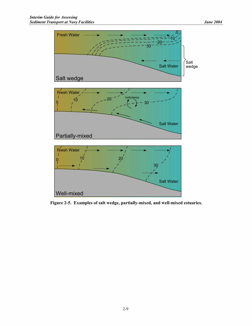
Box 3-1. Online information resources for Tier 1 analysis.
Organization World Wide Web Address NOAA National Geophysical Data Center
Bathymetry and topography http://www.ngdc.noaa.gov/mgg/bathymetry/relief.html
NOAA Office of Coast Survey Nautical charts http://chartmaker.ncd.noaa.gov/
NOAA CO-OPS Tide and current predictions http://co-ops.nos.noaa.gov/tide_pred.html
USGS Water Resources Maps and GIS information http://water.usgs.gov/maps.html
USCOE Links to individual divisions and districts http://www.usace.army.mil/where.html#Maps
NWS Office of Climate, Water and Weather Services
Information dissemination services http://www.nws.noaa.gov/om/disemsys.shtml#FOS
Anthropogenic Activity. Information regarding navigation, dredging, past and future construc-tion activities, and other future use issues should be obtained from various sources including the Navy, USACE, U.S. Coast Guard, and state, regional, or local agencies. Locations, diameters and types of outfalls at or near the site also should be determined.
Existing site conditions should be described as part of the Tier 1 evaluation. If possible, the site should be examined from a boat at high tide and low tide so that shoreline features can be observed. Information that should be noted includes the following:
• Site layout, topography, water body configuration, and identification of features that drain into the water body, including outfalls.
• Nature of the shoreline (e.g., presence of riprap, beaches, and intertidal areas; slope, density and type of vegetation, location of high and low tide lines).
• Dredging and other anthropogenic activity.
• Potential sources of sediment to the water body.
• Flow directions and estimates of velocities.
Any features that are not recorded on maps or in reports should be noted. 3.1.2 Sediment Properties
The characteristics of sediment and the sediment bed often provide insight into the sediment transport environment based on distributions of sediment grain sizes, densities, and contaminants. Biological information also is needed to assess the potential effects of bioturbation.
Sediment Particle Size Distribution, Moisture Content, and Total Organic Carbon (TOC) Content. Sediment type (i.e., particle size distribution) is one of the most important parameters for characterizing sediment transport. Percent moisture data can be used to infer the bulk density of the sediment, which is another critical parameter. If possible, the horizontal and vertical distribution of sediment type (i.e., stratigraphy) should be established.

Interim Guide for Assessing Sediment Transport at Navy Facilities June 2004
3-6
Sediment Contaminant Distribution Data. If available, data on the horizontal and vertical distribution of contaminants potentially can be used to infer sediment transport patterns, if the contaminant source(s) and source loading history are known. Biological Activity. Any existing site-specific or regional data on epibenthic (near bottom dwelling) and benthic (bottom dwelling) biota should be gathered, such as information on organism type and abundance, and seasonal or spatial patterns in biotic activity.
3.1.3 Hydrodynamic Data
Because hydrodynamic processes are always the driving force in sediment transport, these data will often provide a basic level of understanding of the dominant forces in a given site setting. When combined with suspended sediment concentration data, directions and quantities of sediment transport can begin to be determined.
Currents, Tides, Waves, Wind, and Surface Water Runoff. Site-specific or regional data on hydrodynamic forces may be available from a variety of sources including the Navy; USACE; NOAA; the United States Geological Survey (USGS); National Weather Service (NWS); state, regional, and local agencies; and universities (see Box 3-1). Suspended Sediment Concentration Data. Site-specific or regional data on suspended sediment concentrations may be available from the sources listed above. Additionally, available satellite imagery may be used to look at regional trends in relative suspended sediment concentrations.
3.2 Develop Conceptual Site Model
The Navy Sediment Guide (SSC SD, 2003) provides guidance on the development of the overall CSM for a contaminated sediment site. The sediment transport CSM should synthesize all available data, describe a mass balance (i.e., a simple representation of all inputs and outputs to a system), and describe inferred sediment transport patterns (areas of deposition and erosion) based on grain size distribution, contaminant distribution, and geomorphology. The following information should be incorporated into the CSM:
• Describe the site setting and water body characteristics, including the shoreline configuration and bathymetry. Use geographic and geomorphic features to identify likely areas of erosion and deposition.
• Describe the sediment and sediment bed properties. This description should include:
o Sediment type and distribution. Finer-grained sediment (silt and clay) tends to accumulate in depositional areas and coarser-grained sediments tend to occur in higher-energy areas, although fine-grained sediment may be found everywhere in areas with high suspended sediment concentrations.
o Distribution of contaminants (horizontal and vertical). If a single source is responsi-ble for the majority of the contamination, then contaminant concentration gradients can be used to infer the direction of sediment transport away from the source. If the loading history is known, then vertical contaminant concentration gradients can be used to infer sediment accumulation rate (i.e., depth of maximum sediment concen-tration should correspond with period of maximum loading).
o Description of benthic infauna and epifauna.

Interim Guide for Assessing Sediment Transport at Navy Facilities June 2004
3-7
• Identify and describe the most important hydrodynamic processes, and estimate their magnitude and frequency.
o In a fluvial setting, this will be unidirectional currents. o In a marine or estuarine setting, it may be a wave-dominated system, tide-dominated
system, or a combination. o Identify areas where current speeds decrease and are therefore likely to be
depositional.
• Identify sources of particulates to the system. Possible sources of particulates include shore-line erosion, stream or river discharge, local resuspension, advection of particulates from other areas of the water body, and outfalls.
• Define the likely hydrodynamic boundaries of the system.
• Describe any anthropogenic activities that may influence sediment transport processes such as dredging, ship activity, or construction.
• Develop an initial assessment of the mass balance (sediment sources and sinks) and sediment transport patterns (areas of erosion and deposition) based on available information.
The CSM can be presented graphically with an accompanying narrative. An example of a sediment trans-port CSM is presented in Box 3-2. Once developed, the CSM can be used to identify the dominant sedi-ment transport processes at the site based on available site data. The CSM is refined throughout the Tier 1 and Tier 2 evaluations as more data become available.
3.3 Formulate Sediment Management Questions and Tier 1 Study Objectives
The sediment management questions associated with a given site should be formulated concurrently with the development of the CSM. The relevant questions should be used to guide the Tier 1 evaluation. The most common contaminated sediment management questions as related to sediment transport are the following:
• Could erosion of the sediment bed lead to the exposure of buried contamination?
o Under typical conditions? o Under extreme conditions? o Due to prop scour or other anthropogenic activities? o In the future (anticipated change in site use or hydrodynamic conditions)?
• Could sediment transport lead to the redistribution of contamination within the site or
movement of contamination off site?
• Will natural processes lead to the burial of contaminated sediment by relatively clean sediment?
o Is the area depositional? o What is the sediment accumulation rate? o What are the sources of the incoming sediment particles, and are these likely to
change in the future?

Interim Guide for Assessing Sediment Transport at Navy Facilities June 2004
3-8
Box 3-2. Simplified sediment transport conceptual site model.
SOUTH BASIN
Figure 1 shows a site map of South Basin, including existing and historical features. South Basin is a shallow embayment in San Francisco Bay, with depths ranging from 6 ft to less than 2 ft. No streams or rivers enter the South Basin except for Yosemite Creek, a shallow, tidally-influenced channel that only flows approximately once per year. Sediments in South Basin are composed primarily of clayey silt, with silty sand along the shoreline. The primary contaminants of concern are PCBs. The highest concentrations of PCBs in surface sediment are found along the northeastern shoreline of South Basin, adjacent to an onshore landfill. PCB concentrations offshore of the landfill decrease with increasing distance from the shoreline. Sediment core data indicate that the highest PCB concentrations are found in subsurface sediments, which suggests that the original source of PCBs to sediment has been reduced or eliminated. Because PCBs strongly adsorb to sediment particles, sediment transport is expected to be the primary mechanism for their movement over time. PCBs appear to have been historically transported to the offshore area primarily via erosion and transport of contaminated soils in and near the surface of the landfill. Because of its restricted circulation, tidal currents in South Basin are very weak. Waves are likely to be the dominant sediment resuspension mechanism because the basin is shallow and open to the southeast, which is the direction of the prevailing winds during winter storms. The primary source of sediment to the basin appears to be suspended sediment from San Francisco Bay; shoreline erosion may contribute some sediment although the topography adjacent to the basin is relatively flat. Because of the weak circulation in the basin, it is likely to be a net depositional environment with infrequent resuspension events that only act on the surficial sediments (~1-5 cm). A basic CSM for sediment and contaminant transport in South Basin is shown in Figure 2. The dispersal pattern of PCBs, with higher concentrations nearshore and decreasing concentrations offshore, is consistent with wave- and tidally-influenced sediment transport. Storm waves breaking along the shoreline suspend fine, low-density sediments in the nearshore region. A return flow near the bottom of the water column (balancing the shoreward flow due to waves at the surface of the water column) transports the sediments away from the shoreline and into South Basin. Tidally induced currents may facilitate additional transport across the mudflats and extend the influence of waves further offshore during low tide, and potentially carry material further offshore into South Basin. Finally, the deposition of cleaner background sediments transported in from San Francisco Bay and deposited in South Basin results in the dilution and burial of the nearshore and offshore sediments. Biological activity mixes the newly-deposited surface sediment into the sediment bed.
Resuspension due to wave action in shallow waters suspends fine, low density particles
Offshore transport of fine, lower density sediments with bottom return flow due to waves and tides, transports fine sediments from the shore into South Basin, while coarser sediments remain deposited at the shoreline
Net Flux of San Francisco Bay sediments over time cause net sedimentation/deposition in South Basin and Area X
MLLW
Figure 1. Site Map Figure 2. Sediment Transport CSM

Interim Guide for Assessing Sediment Transport at Navy Facilities June 2004
3-9
o What are the physical and chemical properties of the incoming sediment? o At what depth will sediment be unaffected by biological and physical forces? o Are there anticipated changes in site use or hydrodynamic conditions?
• If a site is actively remediated, could sediment transport lead to the recontamination of the
site?
An analysis of the major sediment transport processes (erosion/resuspension, transport, and deposition) at a site is necessary to address any of these questions. Various approaches for characterizing these processes using readily available site data and Tier 1 evaluation methods are described in the following sections. Table 3-2 summarizes the types of data needed to evaluate each of the questions.
3.4 Conduct Tier 1 Analysis
When possible, multiple lines of evidence should be developed in the Tier 1 analysis to support the overall interpretation of sediment transport at a site and facilitate regulatory acceptance of study results. Various approaches (i.e., lines of evidence) for characterizing sediment transport processes are provided below, and the application of the Tier 1 results to common sediment management questions is discussed in Section 3.5. The following is a description of basic calculations that may be performed to obtain a quantitative order-of-magnitude estimate of sediment transport processes. These calculations also can be used to identify critical data gaps and guide additional field data collection at the site. The Tier 1 evaluation relies primarily on analytical techniques (i.e., solved using mathematical formula-tions). The analytical calculations presented below are based on both theoretical (i.e., derived from basic principles) and empirical (i.e., based on measured laboratory or field data) analysis yielding methods use-ful in describing sediment transport processes. More detail on both numerical (i.e., solved using numerical solutions to governing equations) and analytical techniques will be presented as part of Tier 2 along with details on providing empirical data to support these calculations (Section 4.2). 3.4.1 Erosion/Resuspension
The following lines of evidence can be used to characterize sediment stability through the quantification of potential sediment erosion/resuspension at a site:
• Evaluate qualitative indicators (grain size, bathymetry, chemical profiles, etc.) during CSM development to infer if sediments may be erosive (see Section 3.3).
• Calculate the bottom shear stresses and critical shear stress for the system to determine under what conditions erosion is likely.
• Estimate the potential depth of scour based on expected shear stress.
• Evaluate the likelihood and magnitude of extreme events in the system of interest.
Methods for developing these lines of evidence (and for evaluating potential resuspension from ship traffic) are presented below.

Interim Guide for Assessing Sediment Transport at Navy Facilities June 2004
3-10
Estimating Bottom Shear Stress
As described in Section 2.1.2, shear stress is the force produced at the bed as a result of the fluid flow, due to waves and/or currents, applied to an area of sediments. Turbulent shear stress can be simply calculated as:
2uC fρτ = where ρ is the fluid density (kg/m3), Cf is the coefficient of friction, and u is the average fluid velocity (m/s). The coefficient of friction can be calculated for a unidirectional flow by:
2
0
2
2ln
=
zh
kc f
where k is von Karman’s constant (0.42), z0 is the effective bottom roughness (m), and h is the water depth (m). A first estimate of the effective bottom roughness is generally chosen on the order of the grain size diameter of the sediment bed. Using these values, typical ranges for cf are between 0.002 and 0.004 in rivers and estuaries. The coefficients of friction for environments where waves play a larger role involve more effort in their computation and are outlined in more detail in van Rijn (1993), Christoffersen and Jonnson (1985), and Grant and Madsen (1979). The key to estimating shear stress in rivers and estuaries is knowledge of the average velocity over the sediment bed. The average velocity in a river at a given flowrate can generally be obtained through flow rating curves, which give an empirical estimate of velocity from flowrate measurements. The USGS generally has the data for flow rating curves on any river or stream it has gauged. These data provide a good resource for a first estimate of the flow magnitudes expected in the region. NOAA has developed resources for the prediction of tides and associated currents for most of the navigable estuaries and coastal regions in North America. In many navigable locations, NOAA has worked with local agencies to deploy real time current and wave meters for a region. These data provide an excellent resource for determining order of magnitude waves and currents for sites of interest. More sophisticated instrumentation for directly measuring velocity and shear stress is discussed in more detail in the Tier 2 analysis (Section 4.0). In some cases, current and wave data from more sophisticated instruments may be readily available and should be sought out. The error associated with these computations of shear stress come from the error of the velocity used to compute the shear stress and the calculation of the coefficient of friction. The more data available for the calculation of shear stress, the lower the level of uncertainty associated with these calculations. Some sites may have sufficient information available for the Tier 1 analysis. If the data are not available for even basic calculations, instruments and methods for collecting site-specific measurements will need to be used. These instruments and methods are described in Section 4.0 and summarized in Appendix B.

Interim Guide for Assessing Sediment Transport at Navy Facilities June 2004
3-11
Estimating Critical Shear Stress
To predict whether contaminated sediments will be exposed under various flow conditions, the stability of the sediments under those conditions must be determined. As described in Sec-tion 2.1.2, sediment motion is initiated through the shear stress at the bed. The shear stress at which sediment movement begins, the critical shear stress for erosion (τce), can be determined from the Shields curve which gives the critical shear stress for erosion as a function of particle diameter for sediment particles greater than 200 µm (van Rijn, 1993). To calculate the critical shear stress for a particle larger than 200 µm, it is first necessary to calculate the dimensionless particle diameter, d*.
( )3/1
2* 1
−=
υρ gdd s
where d is the median particle diameter (cm), ρs is the density of the particles which is generally assumed to be about 2.6 g/cm3, υ is the kinematic fluid viscosity which is 0.0117 cm2/s for saltwater and 0.0112 cm2/s for freshwater, and g is the acceleration due to gravity (980 cm/s2). Using the d* for the sediment bed, the critical shear stress may be calculated as shown in Table 3-3.
Table 3-3. Critical shear stress for particles larger than 200 µm.
Critical Shear Stress (dynes/cm2) Valid d* Range
( )[ ]gdd sce 1*24.0 1 −= − ρτ 4*1 ≤< d
( )[ ]gdd sce 1*14.0 64.0 −= − ρτ 10*4 ≤< d
( )[ ]gdd sce 1*04.0 1.0 −= − ρτ 20*10 ≤< d
( )[ ]gdd sce 1*013.0 29.0 −= ρτ 150*20 ≤< d
( )[ ]gdsce 1055.0 −= ρτ 150* >d
For smaller cohesive sediment particles (i.e., smaller than 200 µm), the determination of τce is a function of many more sediment variables than particle size, and no single formulation for its calculation exists. For a conservative estimate, 1 dyne/cm2 can be used (Gailani et al., 1991), but this value might vary by almost an order of magnitude for cohesive sediments at various sites (Roberts et al., 1998). For cases requiring a high degree of certainty in critical shear stress measurements, site-specific measurements such as those outlined in the Tier 2 analysis may be required (see Section 4.0). Estimating Resuspension and Depth of Scour
With an initial estimate of τce, the potential for sediment motion can be calculated. For non-cohesive sediments, van Rijn (1993) has developed formulations to describe the transport rates of sediments in wave- and/or current-dominated environments. Depths of scour around structures in non-cohesive sediments are also well outlined in Sumer and Fredsoe (2002).

Interim Guide for Assessing Sediment Transport at Navy Facilities June 2004
3-12
Because contaminants of concern are generally associated with cohesive sediments, cohesive sediment sizes are addressed in more detail. The erosion of cohesive sediments is generally described through empirical formulations as no predictive analytical formulation has been developed to date. One common empirical formulation based on a variation of Partheniades (1965) and refined by Gailani et al. (1991) can be used to obtain order-of-magnitude predictions of sediment erosion. It has been further modified by Ziegler (2002) to estimate the maximum sediment erosion, Emax (mg/cm2), for a specific site based on a maximum expected shear stress, τmax, where all shear stress values are in dynes/cm2:
n
ce
ceAE
−=
τττ max
max
where constant A and exponent n are site-specific parameters. Average values of A and n for eight cohesive sediment systems have been compiled by Ziegler (2002) and are shown in Table 3-4.
Table 3-4. Example erosion parameters for cohesive sediments.
Study Site Constant A (mg/cm2) Exponent n
Upper Hudson River (HydroQual, Inc., 1995) 0.027 3.0 Pawtuxet River (Ziegler and Nisbet, 1994) 0.24 2.0 Watts Bar Reservoir (Ziegler and Nisbet, 1995) 0.1 2.7 Upper Mississippi River 0.11 2.6 Fox River (Lick et al., 1995) 0.75 2.3 Green Bay (Lick et al., 1995) 0.34 2.5 Saginaw River (Lick et al., 1995) 0.053 2.7 Buffalo River (Lick et al., 1995) 0.081 3.1
Average values ± 95% confidence interval 0.21 ± 0.20 2.6 ± 0.3
From this estimate of the maximum erosion at a specific location, the depth of scour in cm, Smax, can be estimated as follows:
sed
ES
ρ1000max
max =
The dry density of the sediments, ρsed (g/cm3), is determined from site-specific data. If no data are available, Ziegler (2002) recommends 1 g/cm3 as a first-order approximation. Extreme Events
Many contaminated sediment sites are located in areas that are depositional most of the time. The most significant risk of contaminant exposure in these systems occurs during large storm or flood events that create conditions under which significant amounts of sediment can be resus-pended. These storm and flood events are termed extreme events and must be considered in any sediment transport evaluation.

Interim Guide for Assessing Sediment Transport at Navy Facilities June 2004
3-13
At riverine sites, the extreme event will typically be a flood. The average number of years between floods of a certain size is the recurrence interval or return period. Flood designations are based on statistical averages, not on the number of years between big floods (USGS, 1996). The term 100-year flood indicates that there is a 1-in-100 chance that a flood of this size will occur in any given year. The actual number of years between floods of any given size varies in response to natural climatic fluctuations. USACE has developed a manual titled “Hydrologic Frequency Analysis” (USACE, 1993) that can be used to evaluate hydrographs and determine the frequency and magnitude of flood events. The values from these analyses can be used to determine the order of magnitude bottom shear stress that may be anticipated during these events. For coastal and estuarine sites, storm activity typically will generate the most extreme event poten-tially affecting sediment transport in the region. USACE has developed the “Coastal Engineering Manual” (USACE, 2002) that outlines how to evaluate the maximum wave and water level con-ditions at a coastal or estuarine site. These values can be used to predict the order of magnitude bottom shear stress that may be expected during these events. It should also be noted the river input into an estuary during an extreme event can significantly alter flow patterns in the region, in which case the analyses for both the riverine and estuarine environments should be combined. Erosion/Resuspension due to Prop Scour
The sediment beds of navigable waterways may be susceptible to scouring action from passing ship traffic. This has presented an engineering challenge in the past and has been studied in some detail. Techniques for the determination of the maximum depth of scour due to ship propellers include those of Sumer and Fredsoe (2002), Blaauw and van de Kaa (1978), Fredsoe (2002), and Hamill et al. (1999). The impacts of ship scour have been investigated by Lindholm et al. (2001) and Michelsen et al. (1998). With known vessel characteristics, empirical methods can be used to predict the depth of scour as a function of time (Liou and Herbich, 1976; Dargahi, 2003).
Summary
The assessment of sediment stability at a site is achieved through the quantification of potential erosion/resuspension of sediments. Once the site has been described in the CSM, typical currents and/or waves at the site can generally be described using the methods outlined above. The range of these values can additionally be determined through an extreme event analysis appropriate for the type of site. With this information, bottom shear stresses typical of the site can be calculated along with a critical shear stress for the sediments present. This information can be used to deter-mine order of magnitude scour depths in regions of interest. Additionally, the potential for erosion due to ship traffic should be considered. For cohesive sediments, a great deal of uncertainty is generally associated with the prediction of an erosion rate and scour depth. Cohesive sediments are known to be highly heterogeneous not only from site to site, but within a localized area. This uncertainty is in addition to any uncer-tainty regarding currents and/or wave forces at the site. Therefore, if an accurate estimate of erosion rates and scour depths is required for the site, a Tier 2 analysis should be considered.
3.4.2 Transport
As discussed in Section 2.1.2, the two fundamental processes responsible for moving sediments from one location to another are advection and diffusion. Advection is the primary process in most systems and therefore is the focus of the Tier 1 analysis. The most useful tool in the initial determination of directions and quantities of sediment transport is a mass balance. A mass balance is a simple representation of all of

Interim Guide for Assessing Sediment Transport at Navy Facilities June 2004
3-14
the inputs and outputs of mass in a system. In an ideal steady-state system, a mass balance can be written as follows:
Sediment mass inflow – Sediment mass outflow + Sediment erosion – Sediment deposition = 0
This basic steady-state mass balance can help determine whether the area of interest is net depositional or net erosional. Mathematically, the steady state mass balance can be expresses as follows:
0=−+− DECQCQ outoutinin The average suspended sediment concentration of the region in mass per unit volume is C; t is the time; Qin and Qout are the incoming and outgoing mass flowrate in volume per unit time; Cin and Cout are the suspended sediment concentrations of the incoming and outgoing water in mass per unit volume; and E and D are erosion and deposition in mass per unit volume per unit time. As a first approximation, the region selected for the CSM can be used as the volume of the area, V. Inflow and outflow from the region, Q, can be estimated for known sources such as rivers and can gener-ally be calculated as Q=A*u where A is the cross-sectional area of the inflow (e.g. river, outfall, etc.) and u is the average velocity through the cross section. The suspended sediment concentrations must be taken from measurements of suspended solids in the system. Erosion and deposition can be estimated as shown in Sections 3.5.1 and 3.5.3, respectively. Conversely, if erosion and deposition rates are unknown, the system inputs and outputs can be balanced to determine if the system is net depositional or net erosional. This can be extremely useful in characterizing a site. Although the information to complete the mass balance with any quantitative certainty will generally not be available in a Tier 1 analysis, it is a useful framework for identifying potential inputs and outputs of sediments and refining the CSM. As an example, a simple bay may be approached from the mass balance framework as shown in Box 3-3. 3.4.3 Deposition
For a Tier 1 analysis, the following lines of evidence can be used to characterize deposition at a site:
• Estimate sediment supply to the site (Section 3.5.2).
• Use bathymetric change over time to determine deposition rate (surveys, dredging records, etc.).
• Use suspended sediment concentrations if available to determine deposition rate.
The measurement of specific radioisotopes in sediment cores can yield estimates of sediment deposition rate; this method is discussed further in Section 4.0 as part of the Tier 2 analysis. At some sites, these data may be available from other research efforts. For navigable waterways, bathymetry records and/or dredging records are generally maintained by the USACE or the local port authority. Sequential bathymetry records can be analyzed to determine volumetric sediment changes throughout an area of interest and/or to simply determine a net change in sediment depth at a specific location over time (see Byrnes et al., 2002; and van der Wal and Pye, 2003). The ability to accurately resolve depth differences between survey dates depends upon the type and consistency of the methods used to collect the data (i.e., single-beam versus multi-beam mapping
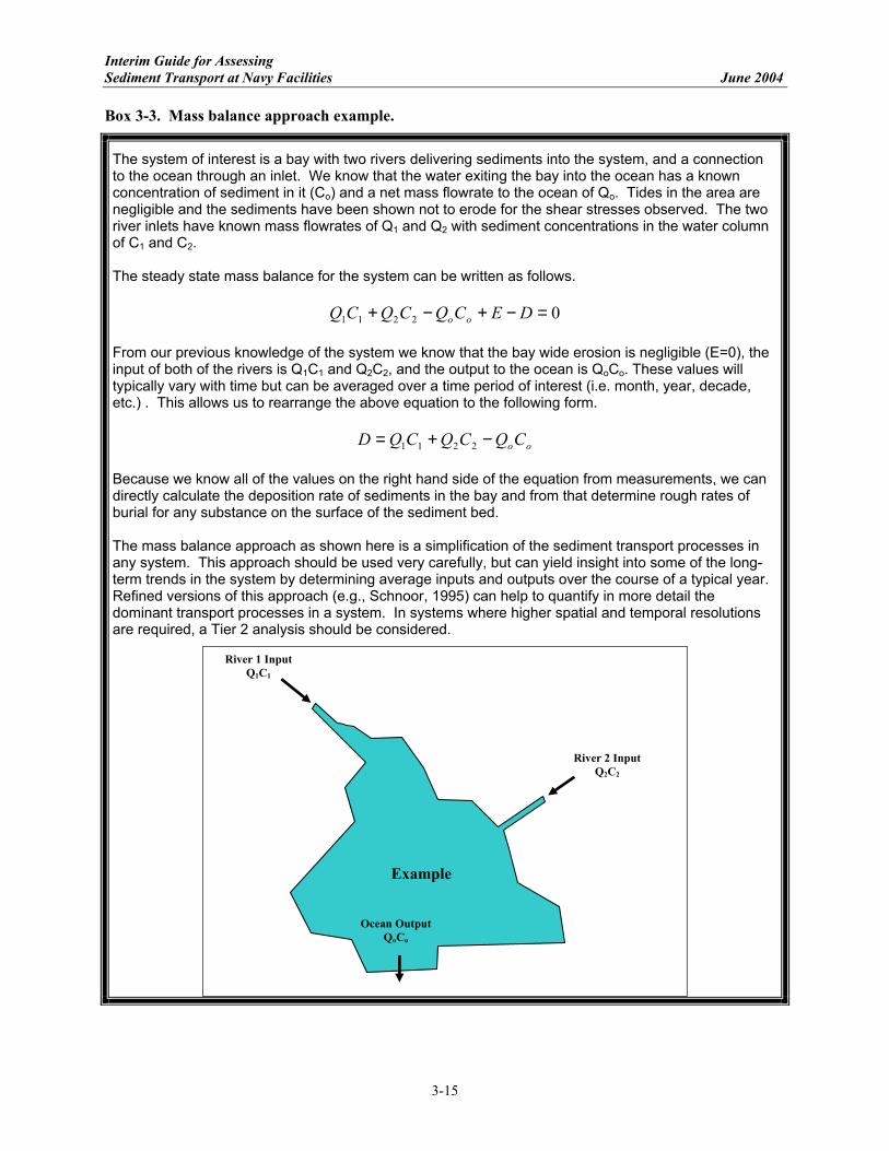
Interim Guide for Assessing Sediment Transport at Navy Facilities June 2004
3-15
Box 3-3. Mass balance approach example.
The system of interest is a bay with two rivers delivering sediments into the system, and a connection to the ocean through an inlet. We know that the water exiting the bay into the ocean has a known concentration of sediment in it (Co) and a net mass flowrate to the ocean of Qo. Tides in the area are negligible and the sediments have been shown not to erode for the shear stresses observed. The two river inlets have known mass flowrates of Q1 and Q2 with sediment concentrations in the water column of C1 and C2. The steady state mass balance for the system can be written as follows.
02211 =−+−+ DECQCQCQ oo
From our previous knowledge of the system we know that the bay wide erosion is negligible (E=0), the input of both of the rivers is Q1C1 and Q2C2, and the output to the ocean is QoCo. These values will typically vary with time but can be averaged over a time period of interest (i.e. month, year, decade, etc.) . This allows us to rearrange the above equation to the following form.
ooCQCQCQD −+= 2211 Because we know all of the values on the right hand side of the equation from measurements, we can directly calculate the deposition rate of sediments in the bay and from that determine rough rates of burial for any substance on the surface of the sediment bed. The mass balance approach as shown here is a simplification of the sediment transport processes in any system. This approach should be used very carefully, but can yield insight into some of the long-term trends in the system by determining average inputs and outputs over the course of a typical year. Refined versions of this approach (e.g., Schnoor, 1995) can help to quantify in more detail the dominant transport processes in a system. In systems where higher spatial and temporal resolutions are required, a Tier 2 analysis should be considered.
Example
Ocean Output QoCo
River 2 Input Q2C2
River 1 Input Q1C1

Interim Guide for Assessing Sediment Transport at Navy Facilities June 2004
3-16
methods; use of same vertical datum and tide correction procedure, etc.). If possible, bathymetric surveys based on the same survey method should be used to ensure data comparability, and the measurement error of the survey method should be noted. Additionally, dredging records can be used to directly determine the volume of sediment deposited in the navigable waterways. All of this information can be used to better characterize the depositional environment (i.e., amount of deposition, type of material, quality of material, and direction of long-term transport). To more quantitatively determine deposition rates at a specific location, the following methodology can be used. In a non-moving fluid where no shear stress is present, the deposition to the sediment bed, D in g/cm2/s, can be described as the product of the settling speed of the sediment particles, ws in cm/s, and the concentration of the sediment in the overlying water, C in mg/L. However, in flowing water, the deposi-tion is affected by the fluid turbulence, which is a function of shear stress. In this case, a probability of deposition, P, can be included in the formulation to account for the effects of the shear stress to yield the following equation:
CwPD s= The settling speed of a sediment particle can be described by Cheng’s (1997) formulation as follows:
( ) 5.12* 52.125 −+= d
dws
ν
where d* is the dimensionless particle diameter calculated in Section 3.4.1 for estimating critical shear stress. This formula gives a generally accurate settling speed based on the sediment particle diameter. The probability, P, would be unity (i.e., 1) in the case of zero flow and would decrease as the shear stress increases. The probability accounts for the decreased chance for deposition as the shear stress increases. For sediment particles, Krone (1962) found that the probability of deposition varied approximately as follows:
≤
−
>=
cscs
cs
for
forP
ττττ
ττ
1
0
When the shear stress at the sediment bed is lower than the critical shear stress for suspension, τcs, parti-cles will begin to deposit onto the sediment bed. For a first guess, τcs can be assumed equivalent to τce. With an approximation of shear stress, settling speed, and suspended sediment concentration, the deposi-tion rate at a location can be estimated. Multiplying the deposition rate over the area of interest A in cm2, and dividing by the bulk density of the deposited sediments, ρsed (~1 g/cm3), gives the burial velocity, Bv, in cm/s (Bv=DA/ρsed). Long-term deposition calculated using this technique is highly dependent on having accurate time series data of sediment concentrations, generally at multiple locations, at the site. Any calculations based on relatively short-term measurements of sediment concentration can yield deposition rates much different from the long-term rates at the site. If an accurate determination of deposition rates at a site is required and the requisite water column data, historic bathymetry, and/or dredging records are not available for a quantitative analysis, a Tier 2 analysis should be considered.

Interim Guide for Assessing Sediment Transport at Navy Facilities June 2004
3-17
3.5 Evaluate Tier 1 Results
The use of the Tier 1 analysis results to address specific sediment management questions is discussed below. When addressing these questions, the uncertainty associated with the Tier 1 estimates must be carefully evaluated, documented, and taken into account. The degree of uncertainty will depend upon the quantity and quality of data used in the Tier 1 analysis. Confidence in the results will be greater if multi-ple lines of evidence point to similar conclusions. The Tier 1 results should be used to refine the sediment transport CSM developed as part of the initial site evaluation. 3.5.1 Could Erosion of the Sediment Bed Lead to Exposure of
Buried Contamination?
The Tier 1 results should be used to describe the conditions under which bottom shear stresses at the site are likely to exceed the critical shear stress, resulting in sediment resuspension and erosion. The Tier 1 analysis may indicate that erosion will occur under some conditions such as spring tides or seasonal storm events, may occur only in an extreme event, or is unlikely to occur under any meteorological conditions. In many cases the extreme event predictions are the most important because contamination would not have persisted at the site for decades (assuming that most contamination occurred from the 1940s to the 1980s) if it was subject to significant erosion under typical conditions. If erosion is possible, then the potential depth of scour can be estimated and compared with the vertical distribution of contamination. If unacceptably high contaminant concentrations are within the possible depth of scour, then it should be assumed that exposure could occur. 3.5.2 Could Sediment Transport Lead to the Redistribution of Contamination
within the Site, or Movement of Contamination Off Site?
If the Tier 1 analysis indicates that sediment resuspension and erosion may occur, then the direction and magnitude of sediment transport should be estimated. Suspended sediments will advect in the direction of currents until reaching a region of lower shear stress, where they will be deposited back onto sediment bed. In tidally-influenced areas, the net direction of transport generally will be in the direction of residual circulation. The accurate characterization of transport generally requires a Tier 2 analysis, although esti-mates can be made on the basis of the mass balance developed in Tier 1. Contaminant distribution data (i.e., concentration gradients) may be the most useful for inferring whether sediment transport is leading to contaminant migration. 3.5.3 Will Natural Processes Lead to the Burial of Contaminated Sediment by
Relatively Clean Sediment?
All lines of evidence that indicate that an area is depositional should be summarized (i.e., based on geo-graphic location, contaminant distribution, mass balance, and/or bathymetric changes). If possible, the sediment accumulation rate should be estimated. The following questions should be addressed: Are sedi-ment sources and quantities likely to change in the future? Do contaminant data indicate that surficial sediments are cleaner than subsurface sediments? At what depth are hydrodynamic forces and bio-turbation unlikely to disrupt sediment profile? Are unacceptable levels of contamination below this depth, or likely to be below this depth in a reasonable amount of time? These questions can be answered with varying degrees of certainty based on the quantity and quality of data available for the Tier 1 analysis.
Interim Guide for Assessing Sediment Transport at Navy Facilities June 2004
3-18
3.5.4 If a Site is Actively Remediated, Could Sediment Transport Lead to the Recontamination of the Site?
In cases where a sediment site has been remediated, recontamination could occur as a result of off-site sources, or from changes in site conditions that would allow on-site contamination to be remobilized (i.e., through changes in site use or hydrodynamic conditions). If potential off-site sources of contamination have been identified, these should be documented in a Watershed Contaminated Source Document (WCSD), which is required as part of Navy sediment policy (Chief of Naval Operations [CNO], 2002). Potential recontamination from off-site sources should be documented in the Record of Decision for the site before the response action is taken. The mass balance can be used to qualitatively evaluate the effects of changes in future hydrodynamic conditions or site use. For example, construction of a navigational channel near the remediated area could increase current speeds and the potential for erosion. Additionally, the potential effects of the remedial approaches themselves (e.g., construction of a cap) on the site hydrodynamics should be evaluated in the FS.
3.6 Determine Need for Tier 2 Analysis
After the sediment management questions have been addressed, the need for a more refined Tier 2 evalua-tion must be evaluated. The decision about whether to conduct a Tier 2 analysis must take into considera-tion the level of uncertainty associated with the Tier 1 analysis, and the potential consequences both from a risk and cost perspective of making an incorrect site management decision based on the Tier 1 analysis. Possible scenarios include the following:
• In general, if a site is relatively large and complex and the anticipated costs for remediation are high, then a Tier 2 analysis will be required to refine the sediment transport CSM and reduce the uncertainty associated with site management decisions, particularly if in situ approaches (i.e., monitored natural recovery or capping) are expected to be a component of the remedy.
• If a site is relatively small and the anticipated cost of remediation is relatively low, then a Tier 2 analysis may not be necessary.
• If the Tier 1 analysis indicates that sediment transport is not likely to be a major factor in contaminant migration, the site risks are relatively low to moderate, and the uncertainty is relatively small, then a Tier 2 analysis may not be warranted. However, if the uncertainty associated with the same analysis is relatively high, then a Tier 2 analysis should be considered.
• If the Tier 1 analysis indicates that a site is stable, then the consequences of contaminant dispersal in the future due to sediment transport should be considered in case the conclusion is incorrect. If the consequences are unacceptable, then a Tier 2 analysis should be performed to reduce uncertainty.

Interim Guide for Assessing Sediment Transport at Navy Facilities June 2004
4-1
4.0 TIER 2 EVALUATION
When the results of a Tier 1 investigation indicate that remedial action is likely, a more detailed analysis may be needed to support evaluation of alternatives, particularly in situ approaches (i.e., capping and natural recovery). The goal of a Tier 2 evaluation is to address common sediment management questions with a higher degree of certainty using targeted, site-specific data and more sophisticated data analysis methods than for Tier 1 investigations. Tier 2 evaluations generally are conducted in latter stages of the RI or early stages of the FS. Additional site-specific, focused data collection is generally required to support Tier 2 analyses. Detailed sediment contaminant distribution mapping also may be useful and can be conducted concurrently to better define the area and volume of sediment to be considered in the FS. Tier 2 methods are described in less detail in this Interim Guide than the Tier 1 methods. Tier 2 will be presented in more detail in the Final Guide, including presentation and discussion of the results of site demonstrations that apply many of the tools and methods described in this section and Appendix B. The Final Guide will identify the most important types of Tier 2 data to collect to address specific sediment management questions. The Final Guide also will provide a more detailed description of how Tier 2 data are used in numerical models.
4.1 Collect Tier 2 Data
The refined CSM and a sensitivity analysis of the Tier 1 results can be used to identify the greatest sources of uncertainty associated with sediment transport estimates. The Tier 2 data collection effort should be based on the key data gaps identified at the end of the Tier 1 evaluation. The scope of the data collection effort should be developed through application of the seven step data quality objective (DQO) process (USEPA, 2000). Example DQOs for a Tier 2 sediment transport evaluation are provided in Table 4-1. Examples of Tier 2 data sources and data collection methods are summarized in Table 3-1. Appendix B provides more detail on tools and technologies available for Tier 2 data collection, including advantages, limitations, and cost considerations.
Table 4-1. Example Tier 2 data quality objectives for South Basin.
STEP 1: State the Problem Sediments in South Basin are contaminated with PCBs and may pose an unacceptable risk to human health and the environment. Additional data are needed to characterize sediment transport, refine the conceptual site model (CSM), and evaluate the feasibility of various remedial alternatives (i.e., removal, monitored natural recovery, and in situ capping). STEP 2: Identify the Decision 1. Is the sediment bed likely to erode under typical and extreme hydrodynamic conditions, and to what depth? 2. Will natural processes effectively cap contaminated sediments? STEP 3: Identify Inputs to the Decision 1. Existing site-specific data on the horizontal and vertical distribution of PCBs sediment, and current velocities
in South Basin in summer and winter. 2. Vertical profiles of bulk density, grain size, and erosion rates for sediment cores obtained from Sedflume
sampling to characterize stability of the sediment bed. 3. Sediment accumulation rate (age profile) from radioisotope data (210Pb, 137Cs, 7Be, 237Th). 4. PCB concentration data for sediment particles settling on the sediment bed as collected in sediment traps. 5. Thickness of the biologically active zone from published literature, and estimation of the mixed depth from
site-specific radioisotope data (210Pb, 137Cs, 7Be, 237Th). STEP 4: Define the Study Boundaries The study area is bounded by the toe of the embankment along the South Basin shoreline. Only soft sediment
will be sampled. Sediment cores will be collected in South Basin from Yosemite Creek to Candlestick Point. The vertical limit of the study area is 1 m, because previously collected core data indicate that PCB concen-
trations drop significantly below 0.7 m. Cores for radioisotope analysis will be collected to a depth of 1.5 m.
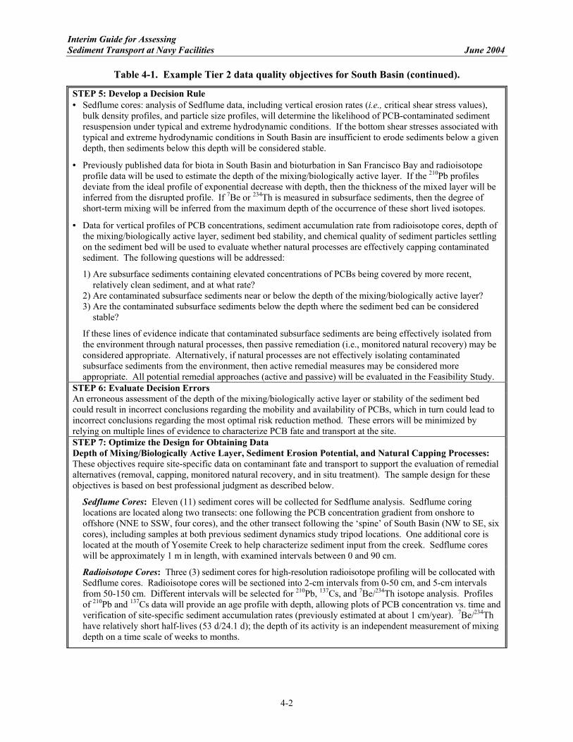
Interim Guide for Assessing Sediment Transport at Navy Facilities June 2004
4-2
Table 4-1. Example Tier 2 data quality objectives for South Basin (continued).
STEP 5: Develop a Decision Rule • Sedflume cores: analysis of Sedflume data, including vertical erosion rates (i.e., critical shear stress values),
bulk density profiles, and particle size profiles, will determine the likelihood of PCB-contaminated sediment resuspension under typical and extreme hydrodynamic conditions. If the bottom shear stresses associated with typical and extreme hydrodynamic conditions in South Basin are insufficient to erode sediments below a given depth, then sediments below this depth will be considered stable.
• Previously published data for biota in South Basin and bioturbation in San Francisco Bay and radioisotope profile data will be used to estimate the depth of the mixing/biologically active layer. If the 210Pb profiles deviate from the ideal profile of exponential decrease with depth, then the thickness of the mixed layer will be inferred from the disrupted profile. If 7Be or 234Th is measured in subsurface sediments, then the degree of short-term mixing will be inferred from the maximum depth of the occurrence of these short lived isotopes.
• Data for vertical profiles of PCB concentrations, sediment accumulation rate from radioisotope cores, depth of the mixing/biologically active layer, sediment bed stability, and chemical quality of sediment particles settling on the sediment bed will be used to evaluate whether natural processes are effectively capping contaminated sediment. The following questions will be addressed:
1) Are subsurface sediments containing elevated concentrations of PCBs being covered by more recent, relatively clean sediment, and at what rate?
2) Are contaminated subsurface sediments near or below the depth of the mixing/biologically active layer? 3) Are the contaminated subsurface sediments below the depth where the sediment bed can be considered
stable?
If these lines of evidence indicate that contaminated subsurface sediments are being effectively isolated from the environment through natural processes, then passive remediation (i.e., monitored natural recovery) may be considered appropriate. Alternatively, if natural processes are not effectively isolating contaminated subsurface sediments from the environment, then active remedial measures may be considered more appropriate. All potential remedial approaches (active and passive) will be evaluated in the Feasibility Study.
STEP 6: Evaluate Decision Errors An erroneous assessment of the depth of the mixing/biologically active layer or stability of the sediment bed could result in incorrect conclusions regarding the mobility and availability of PCBs, which in turn could lead to incorrect conclusions regarding the most optimal risk reduction method. These errors will be minimized by relying on multiple lines of evidence to characterize PCB fate and transport at the site. STEP 7: Optimize the Design for Obtaining Data Depth of Mixing/Biologically Active Layer, Sediment Erosion Potential, and Natural Capping Processes: These objectives require site-specific data on contaminant fate and transport to support the evaluation of remedial alternatives (removal, capping, monitored natural recovery, and in situ treatment). The sample design for these objectives is based on best professional judgment as described below.
Sedflume Cores: Eleven (11) sediment cores will be collected for Sedflume analysis. Sedflume coring locations are located along two transects: one following the PCB concentration gradient from onshore to offshore (NNE to SSW, four cores), and the other transect following the ‘spine’ of South Basin (NW to SE, six cores), including samples at both previous sediment dynamics study tripod locations. One additional core is located at the mouth of Yosemite Creek to help characterize sediment input from the creek. Sedflume cores will be approximately 1 m in length, with examined intervals between 0 and 90 cm.
Radioisotope Cores: Three (3) sediment cores for high-resolution radioisotope profiling will be collocated with Sedflume cores. Radioisotope cores will be sectioned into 2-cm intervals from 0-50 cm, and 5-cm intervals from 50-150 cm. Different intervals will be selected for 210Pb, 137Cs, and 7Be/234Th isotope analysis. Profiles of 210Pb and 137Cs data will provide an age profile with depth, allowing plots of PCB concentration vs. time and verification of site-specific sediment accumulation rates (previously estimated at about 1 cm/year). 7Be/234Th have relatively short half-lives (53 d/24.1 d); the depth of its activity is an independent measurement of mixing depth on a time scale of weeks to months.

Interim Guide for Assessing Sediment Transport at Navy Facilities June 2004
4-3
Table 4-1. Example Tier 2 data quality objectives for South Basin (continued).
STEP 7: Optimize the Design for Obtaining Data (continued) Sediment Traps: Two sets of sediment traps will be collocated with two of the radioisotope profile cores to provide complementary data on the quantity and quality of sediment particles settling on the sediment bed. A third set of sediment traps will be deployed at the entrance to South Basin, at the location of the previous sedi-ment dynamics study tripod location. Two sediment traps will be deployed at each location to provide suffi-cient sample material in the event that one of the traps fails. Sediment from both traps at each location will be combined into a single sample. Sediment traps will be deployed for one year to assess seasonal variability. Each deployment period will be three months in duration, with the initial deployment in October 2003 and turnaround cruises in January, April, and July 2004.
Depth of Mixing/Biologically Active Layer: A literature review will be conducted to provide information on a range of bioturbation depths for a number of different species and habitats in San Francisco Bay. Radioisotope profile data from sediment cores will also be used to support an estimation of total mixed depth.
4.2 Conduct Tier 2 Analysis
The Tier 2 analyses should be focused based on Tier 1 findings, the refined CSM, and relevant sediment management questions. Tier 2 analyses should provide a description of more complex and site-specific sediment transport processes. When possible, multiple lines of evidence should be used in Tier 2 to support the overall interpretation. Generally, a Tier 2 analysis will focus on site-specific data collection to support modeling efforts. These modeling efforts can be analytical and/or numerical. 4.2.1 Erosion/Resuspension
If sediment erosion and/or resuspension have been identified in Tier 1 as one of the driving forces for sediment transport, additional data/analyses may be done to more accurately quantify this parameter. One of the key measurements in predicting sediment erosion at a site is to directly measure the critical shear stress and sediment erosion rate with depth. These measurements will allow a quantitative estimation of sediment erosion under both typical and extreme conditions based on site-specific hydrodynamic and sediment strength data. Several types of laboratory and in situ flume techniques exist to measure these parameters, including annular flumes, straight flumes, and shaker flumes. Table 4-2 summarizes some of the more common research and commercially-available methods for the measurement of sediment stabil-ity parameters. All of the devices measure critical shear stress of erosion of cohesive sediments; the pri-mary differences between them are related to whether they can be used in situ, the applicable shear stress range, and the depth to which erosion properties can be measured. Appendix B provides additional information on advantages, limitations, and relative costs for some of the more readily available devices. In combination with measurements of critical shear stress and erosion rates, the forces driving erosion events must be characterized. This analysis will be site-specific, and can include river discharge, tidal currents, and wave action. At sites where wave action is a driver of sediment transport, wave energy can be measured. Waves contribute to sediment transport by increasing the bed shear stress and by mixing and transporting sediment that is already suspended. Most commonly, these data can be used in conjunction with measurements of critical shear stress and erosion rate to predict the erosion of sediments as a result of wave action. Erosion and resuspension events in riverine and estuarine environments can also be directly measured at a site by collecting both spatial and time-series measurements of suspended sediment concentrations and current velocity in the water column. These types of measurements can allow determination of the current velocity at which sediments become resuspended, the concentration of sediment in suspension,

Interim Guide for Assessing Sediment Transport at Navy Facilities June 2004
4-4
Table 4-2. Comparison of various sediment stability measurement devices (courtesy of Sandia National Laboratories).
Device
Flow Conditions
(over sediment surface)
In Situ
Ex Situ
Transport Measured τcs
ErosionRate
Sediment Type
Depth Measured
ShearStressRange
Straight Flume
Linear/ Oscillatory
Yes Yes Total Load Yes Yes Clay/Silt/ Sand
Surficial Layers
0-4 PA
Annular Flume / Sea Carousel
Linear Yes Yes Suspended Load Only
Yes No Clay/Silt/ Sand
Surficial Layers
0-1 PA
Shaker Unknown No Yes Suspended Load Only
Yes No Clay/Silt/ Sand
Surficial Layers
0-1 PA
Sedflume Linear No Yes Total Load Yes Yes Clay/Silt/ Sand
0-3 m 0-10+ PA
ASSET Fume
Linear No Yes Suspended And
Bedload
Yes Yes Clay/Silt/ Sand
0-3 m 0-10+ PA
SEAWOLF Flume
Linear/ Oscillatory
No Yes Total Load Yes Yes Clay/Silt/ Sand
0-3 m 0-10+ PA
and the height in the water column to which sediments are being carried. The signature of the sediment signal may also indicate whether the sediments are being resuspended by tidal currents (Figure 4-1), advection, or storm events (Figure 4-2). Extreme weather events, such as floods and hurricanes, may have significant effects on sediment transport at a site. To predict the impact of extreme events, a statistical analysis can be performed to quantify the probability and magnitude of events and their effect on erosion, transport, and deposition at a site. Because extreme conditions are typically difficult to estimate accurately and often have large economic implications, a number of different techniques have been developed to determine the probability and magnitude of extreme events in different systems (USACE, 1993 and 2002). Another factor affecting the stability of bed sediments is biological activity in the surface sediments. Biological activity can have a significant effect on the physical properties of the sediments both by increasing sediment strength during tube-building activities and decreasing strength and cohesion during burrowing. Changes in sediment stability resulting from biological activity can be estimated from detailed biological assessment, sediment profile images, redox profiles, and measurement of short-lived isotopes. Anthropogenic activities such as ship movement and dredging also may affect the erosional characteris-tics of a site. The propellers of ships generate a high intensity current, which can scour marine sediments to significant depths. If the sediments in the region of scour are contaminated, there is a significant potential for contaminant release. The subsequent transport of these sediments in littoral zones and side channels also may adversely affect ecosystems over larger areas.

Interim Guide for Assessing Sediment Transport at Navy Facilities June 2004
4-5
Figure 4-1. Tidal time-series measurements of suspended sediment concentration (top) and along-channel current velocity (bottom) from the ACE Basin, SC show that sediments are resuspended
during maximum flood and ebb currents.
TSS (mg/l)
PaletaCreek
Chollas Creek 0
50
100
Figure 4-2. Spatial measurements in San Diego Bay, CA show evidence of a
stormwater plume from a small urban creek.

Interim Guide for Assessing Sediment Transport at Navy Facilities June 2004
4-6
As stated in Section 3.4.1, the sediment beds of navigable waterways may be susceptible to scouring action from passing ship traffic. Currently available methods for the estimation of prop scour rely on empirical sediment stability relations for sands (e.g., non-cohesive sediments), which have been demon-strated to be of limited use in determining the resistance of natural sediments to scour. The Sedflume and related devices are effective tools that may be used to measure sediment erosion (or scour) rates under various flow conditions. 4.2.2 Transport
The direct measurement of suspended sediment transport at a site may include additional data on currents, waves, and suspended sediment concentration. These data should be collected over time scales (i.e., tidal time scales, seasonal time scales) that correspond to the hydrodynamic forces of interest. Time-series measurements of current velocity and suspended sediment concentration can be used to determine the net flux of sediments past a given point (Figure 4-3). A calculation of the net flux will provide information on the direction of net sediment movement.
z, depth
u, along-channel
v, across-channel
∆v
∆u∆z
uc
F
Figure 4-3. A schematic of net sediment flux through a parcel of water.
The instantaneous sediment flux, F, through a section perpendicular to the mean flow can be calculated by using the equation:
∫ =∆⋅=h
0
uchzucF
where u is the along-channel velocity, c is suspended-sediment concentration, z∆ is the depth interval between measurements, and h is the total depth (Dyer, 1997). The instantaneous fluxes of sediment can also be evaluated over time (i.e., a tidal cycle), yielding a net mean flux, Q (Dyer, 1997). The angle brackets denote averaging over the total depth, and an overbar (i.e., Q ) denotes an average over time. The calculated value for the net sediment flux can also be used to refine the mass balance for the system (Section 3.4.2).

Interim Guide for Assessing Sediment Transport at Navy Facilities June 2004
4-7
If bed transport is suspected, regional bathymetry data may be collected over time to determine the net movement of sediments by tracking bedforms. The direction of sediment movement can sometimes be determined based on the shape of bedforms. Direct measurement of bedload transport is difficult, however, and many different equations have been developed to predict the bedload flux (van Rijn, 1993). 4.2.3 Deposition
In Tier 2, site-specific deposition processes can be characterized in more detail through use of radio-isotope dating techniques and/or sediment traps. Particle settling characteristics can also be evaluated. Radioisotope profiling is a useful tool that can be used to date sediment sections in an undisturbed core and determine the net accumulation rate of sediments (USGS, 1998). The age of sediments is calculated by knowing the original concentration of the isotope and measuring the percentage of the remaining radioactive material after decay has occurred. In an undisturbed sediment core, the activity of the isotope will decrease exponentially with increasing depth until it reaches a background level (Figure 4-4). How-ever, mixing of sediment by organisms or other processes will disrupt the smooth profile and reduce the accuracy of the estimated dates and sediment accumulation rates. Commonly used radioisotope tracers are 210Pb, 137Cs, 14C, 7Be, and 234Th. Each isotope has a different half-life and can be used to detect sedimentary accumulation over different timescales.
Source: USGS, 1998.
Figure 4-4. Lead-210 profile: ideal and actual from Florida Bay.
210Pb forms by the radioactive decay of its gaseous parent, 222Rn (222Rn forms from the decay of radium). 210Pb is removed from the atmosphere by precipitation, and is rapidly adsorbed to and deposited with sediment particles. This flux of 210Pb from the atmosphere produces a concentration of “unsupported” 210Pb (i.e., a concentration which exceeds the “supported” concentration resulting from radioactive decay of the sediment itself). The half-life of 210Pb is 22.3 years, and dates of sediment deposition can be esti-mated by determining decrease of 210Pb activity with depth. In an undisturbed sediment core, “unsup-ported” 210Pb activity will decrease exponentially with increasing depth until it reaches the supported 210Pb level. The rate of sediment accumulation in cm/yr can be calculated based on the dated sediment column. The sedimentation rate in grams of dry sediment per year per cm2 also can be calculated if the wet and dry densities of the sediment are determined.

Interim Guide for Assessing Sediment Transport at Navy Facilities June 2004
4-8
137Cs was present in the fallout from atmospheric nuclear tests, and first appeared in sediment cores around 1952-1955. Deposition of 137Cs peaked in 1963-1964. In an undisturbed sediment core, 137Cs activity levels will reflect 137Cs production during the period of atmospheric nuclear testing, with an initial appearance in the early to mid-1950s, a peak in the early 1960s, and a decrease in the early 1970s after atmospheric testing was halted. 14C was also a byproduct of atmospheric nuclear testing. The amount of bomb-produced 14C can be determined by comparing present activity to the 1950 carbon activity, which is by convention the baseline used for radiocarbon dating (USGS, 1998). Naturally-occurring 14C can be used to date organic material between 100 and 70,000 years old. 7Be and 234Th can be used to date sediments in shorter time frames and provide information about short-term surface sediment mixing. 7Be is formed by the atmospheric bombardment of atmospheric nitrogen and oxygen. It has a half-life of 53 days, and can be used to date sediments with an age up to one year. 234Th forms from the decay of 238U. 234Th has a half-life of 24 days. The reliability of the ages obtained from radioisotope dating methods depends on the degree to which the assumptions underlying the method are met. Some of the key assumptions are as follows:
• The sediment accumulation rate is constant (i.e., sedimentation processes are constant). How-ever, natural sedimentation is commonly episodic rather than continuous, and sedimentation rates are likely to fluctuate rapidly over short periods of time in watersheds where rapid development has taken place.
• The grain size of the deposited sediment is uniform. Uncertainty will be introduced if samples are taken from core segments with unequal grain sizes.
• The background (i.e., unsupported) level of activity is known. If this information is not available from regional studies, then an assumption regarding the background activity level must be made.
Because of the inherent uncertainty in the ages obtained from radioisotope analysis, other information (geological, chemical, and historical) should be taken into consideration when interpreting the data. Detailed stratigraphic information can be used in conjunction with the radioisotope data to infer the depositional characteristics of the site. Contaminant profiles in the sediment core may also be used as a reference for age-dated core sections. For example, a historical contaminant spill at a site may be evident as a spike at depth in the chemical profile. Dates obtained from one age-dating method (e.g., 137Cs) can be used to validate the dates derived by another method (e.g., 210Pb). Chillrud et al. (2003), Fuller et al. (1999), and Aller and Cochran (1976) are examples of studies based on radioisotope analysis of sediment cores. A sediment trap is a device deployed in the water column that collects a representative sample of the material settling through the water column before it passes to a greater depth and is incorporated into the sediment bed (Figure 4-5). Sediment trap data can be used to characterize the flux of sinking particles in a system, which may relate to deposition. The difference between the gross downward flux of sediments and the net sediment accumulation rate (i.e., from radioisotope dating) also can be used to approximate the flux due to sediment resuspension (Jensen et al., 1990; Perjup et al., 1996). Contaminant chemistry measurements from sediment traps can also be very useful in determining the source(s) and quality of incoming sediments. Sediment traps were first designed for use in the deep ocean where current velocities are very small (<0.1 m/s). However, recent work has been done to assess the use of sediment traps in shallower,

Interim Guide for Assessing Sediment Transport at Navy Facilities June 2004
4-9
Figure 4-5. Diver-deployed sediment trap.
high-energy environments. Many different designs for sediment traps have been used over the last few decades, with most designs falling into the following five broad categories (Gardner, 1980):
• Cylinders • Funnels • Wide-mouth jars • Flasks and Tauber traps (mouth of container < body) • Basin/tray-like containers (width >> height).
Studies have shown that cylinders are the most efficient sediment trap shape (Hargrave and Burns, 1979; Bloesch and Burns, 1980; Blomqvist and Hakanson, 1981; Butman, 1986), whereas funnel and tray shaped traps tend to under-collect sediment (Pennington, 1974; Reynolds and Godfrey, 1983) and Tauber traps tend to over-collect sediment (Pennington, 1974). Additional factors affecting the efficiency of a sediment trap are the aspect ratio (height:diameter ratio) of the trap and the addition of brine. For example, upwelling and resuspension of sediments in the trap may occur if the height:diameter ratio is too low. In high-energy environments, an aspect ratio between 3 and 5 is recommended (White, 1990). Traps are commonly partially filled with a brine solution (~50 psu) to prevent sediments from being resuspended by currents (Nodder and Alexander, 1999). Dye may be added to the brine solution so that the interface can be seen and to determine if the brine layer has been mixed with the overlying water during deployment. Biocides (i.e., formalin or sodium azide) also can be added to deter animals from eating or removing sediment from the trap.

Interim Guide for Assessing Sediment Transport at Navy Facilities June 2004
4-10
Particle size characteristics may also affect the deposition of sediments in an aquatic environment. The settling speed of a natural sediment particle can be described by Cheng’s (1997) formulation as follows:
( ) 5.12* 52.125 −+= d
dws
ν
where d* is the dimensionless particle diameter calculated in Section 3.4.1 for estimating critical shear stress. This formula gives a generally accurate settling speed based on the sediment particle diameter. In estuarine waters in particular, suspended sediments are prone to flocculate, or aggregate, into larger particles. By neglecting to consider the aggregation of particles in fine-sediment environments, an underestimation of particle settling velocities of up to an order of magnitude may result (Kineke and Sternberg, 1989). Techniques have been developed to predict flocculation and determine resulting particle sizes (Burban et al., 1990). Post-depositional processes (i.e., bioturbation) may alter sedimentary structures, making the analysis of the depositional history difficult. As noted above, these processes can be characterized through detailed biological assessment, sediment profile imaging, redox profiling, and the measurement of short-lived radioisotopes. 4.2.4 Numerical Modeling
Numerical models are useful tools that can provide a more complete understanding of the transport and fate of sediments than can be provided by empirical data (from field or laboratory) alone. However, they can be expensive to apply at complex sediment sites because of the large quantities of site-specific data and modeling experience that is needed. Modeling of contaminated sediments, just as with other model-ing, should follow a systematic planning process that involves examination of data quality objectives (or other measures), uncertainty, and specific hypothesis. In most cases, models are expected to complement environmental measurements and address gaps that exist in empirical information. Ziegler (2002) presents a good discussion of Tier 2 modeling approaches. Models can be used to assess the historical stability of sediment and the future of sediment stability under a variety of events or conditions. Confidence in a model’s predictions is based largely on the amount of site-specific data available, and the error associated with predicting the natural variability in the system. Because predictions are accompanied by uncertainty, validation often needs to be performed in order to demonstrate the numerical accuracy of the prediction (e.g., via confidence intervals). Typically, confi-dence decreases with the degree of extrapolation involved in predicting the design event (e.g., long-range predictions). Once a sediment transport model is calibrated properly and validated, the model can be used as a management tool to quantitatively and objectively evaluate the efficacy of various remedial alternatives. A wide range of models have been developed with varying levels of complexity. The models described here have been broken down into three types. A few examples of modeling frameworks are presented below for Types 2 and 3. Characteristics of various hydrodynamic and coupled hydrodynamic/sediment transport models also have been summarized by the USGS (2002).
• Type 1 – Control volume models (i.e., box models).
• Type 2 – Simplified hydrodynamic and sediment transport: one-dimensional (1-D) simula-tions of flow and sediment transport.

Interim Guide for Assessing Sediment Transport at Navy Facilities June 2004
4-11
• Type 3 – Higher order hydrodynamic and sediment transport models: two-dimensional (2-D) or three-dimensional (3-D) transport models.
Type 1
Most Type 1 models are designed to solve the mass continuity equation (advective/dispersive transport) employing a “well-mixed” controlled volume approach. These models are also commonly referred to as “box models”. Although the number of dimensions and scales of resolution that can be specified with these models is very flexible, the hydrodynamic and sediment transport portions of the model are typically very general (i.e., coarse resolution). Although models of this type are widely available, well-developed, and provide a good descriptive ability, they are generally not suitable for accurate predictions of sediment transport because they do not resolve fine scale transport processes critical for accurate predictive capability. These relatively simple models are usually used for preliminary screening level analyses at a site and are a common framework for contaminant fate and transport efforts. Type 2
Type 2 models simulate one-dimensional flow and sediment transport using simplistic mechan-ical descriptions of resuspension and deposition. These models differentiate between non-cohesive and cohesive sediments and take into account bed armoring effects, multiple particle size classes, and spatially variable bed properties. Generally, these models require almost as much site-specific data as Type 3 models, although less modeling experience is needed to apply them. Interpretation requires as much (if not more) knowledge of hydrodynamics and sediment transport as that for multi-dimensional models. Examples of Type 2 models are HEC-6, Gener-alized Stream Tube Model for Alluvial River Simulation (GSTARS) 2.1 and Environmental Fluid Dynamics Code (EFDC)-1D. Each of these models is described in more detail below.
HEC-6 (USACE, 1990)
HEC-6 is a 1-D movable boundary open channel flow model designed to simulate and predict changes in river profiles resulting from scour and/or deposition. It can be used to analyze networks of streams, channel dredging, and various levee and encroachment alternatives. HEC-6 simulates the capability of a stream to transport sediment, given the yield from upstream sources. This computation of transport includes both bed and suspended load as described by Einstein’s bedload function (Einstein, 1950). Effects of the creation and removal of an armor layer can also be simulated. GSTARS 2.1 (Molinas and Yang, 1986)
GSTARS 2.1 is a hydraulic and sedimentation numerical model developed to simulate flows in rivers and channels with or without movable boundaries. The bed sorting and armoring algorithm used by GSTARS 2.1 is based on sediment size fractions. The model also accepts tributary inflows of water and sediment. EFDC-1D (TetraTech, 2001)
The EFDC-1D is a control volume-based 1-D hydrodynamic and sediment transport model for river networks. It can simulate bidirectional unsteady flows and can accommodate unsteady inflows and outflows, lateral inflows and withdrawals, groundwater-surface water interaction, evaporation, and direct rainfall. For sediment transport, the model includes settling, deposition, and resuspension of multiple size classes of cohesive and non-cohesive sediments. A bed consolidation model is implemented to predict time variations of bed

Interim Guide for Assessing Sediment Transport at Navy Facilities June 2004
4-12
depth, void ratio, bulk density, and shear strength. The sediment bed representation is dynamically coupled to the cross-sectional area representation in order to account for area changes due to deposition and resuspension.
Type 3
In general, Type 3 models employ more detailed descriptions of resuspension and deposition processes that are developed from experimental results. Like Type 2 models, Type 3 models can differentiate between non-cohesive and cohesive sediments and include bed armoring effects, particle size classes, and spatially variable bed properties. They are used to assess 2-D or 3-D water column transport and are coupled to sophisticated hydrodynamic models. They also incorporate the effects of currents and waves on bottom shear stress. In general, these models are capable of producing accurate simulations of sediment transport, assuming an adequate amount of site-specific and calibration data are entered into the model. Because they are relatively complicated models, an experienced engineer or scientist needs to be responsible for applying or interpreting these models. Several Level 3 models are described in detail below.
EFDC (TetraTech, 2000)
The EFDC model is a public domain modeling system for simulating 3-D flow, transport, and biogeochemical processes in surface water systems, including rivers, lakes, estuaries, reservoirs, wetlands, and nearshore coastal regions. The EFDC model solves the 3-D, vertically hydrostatic, free surface, turbulent averaged equations of motion for a variable density fluid. EFDC uses curvilinear-orthogonal horizontal and sigma vertical grids and Mellor-Yamada 2.5 turbulence closure (Mellor and Yamada, 1982). It also includes drying and wetting, wave-induced currents, vegetation resistance, and hydraulic structures. The model has a number of sediment transport capabilities including:
1) Multiple size classes of cohesive and non-cohesive sediment; 2) Multi-layer sediment bed with armoring and consolidation; 3) Sediment processes function library allowing many different settling, deposition,
resuspension, armoring, and bedload transport formulations; 4) Hindered settling of non-cohesive sediment; 5) Concentration and shear (or stress) dependent settling of cohesive sediment; 6) Non-cohesive bed exchange; 7) Cohesive sediment deposition resuspension. COMAPS (Welsh et al., 2000)
The COupled MArine Prediction System, or COMAPS, uses the following combination of wave, circulation, sediment transport, and boundary layer models: 1) CH3D-SED (Spasojevic and Holly, 1994) for circulation and sediment transport; 2) CONS for sediment consolidation; 3) WAM (WAMDI, 1988) and SWAN for wind-wave interactions; 4) WCBL (Lee, 1992; Keen and Glenn, 1998) for the wave-current bottom boundary layer; 5) SEAF for shore erosion; 6) EPT for Eulerian particle tracking; and 7) RT3D-SED for radioactivity-toxicant transport. In addition to is ability to perform quantitative, source-specific, sediment flux and loading analyses, COMAPS can also be used to: (1) assess the impacts of bed armoring, replacement,

Interim Guide for Assessing Sediment Transport at Navy Facilities June 2004
4-13
and sequestration; (2) recreate “virtual sight” for amphibious operations; (3) perform a wave-length-dependent light field penetration for ecosystem analysis; (4) identify a severe sea state hazard located near shore; (5) assess design applications including scenario testing; (6) assess the real-time disposal of dredged material/toxins; and (7) interpret acoustic instrument response data. SEDZL (Zeigler and Lick, 1986)
SEDZL models have been tested in a large number of environments including rivers, lakes and bays, coastal bays and lagoons, and coastal ocean regions. Typically two sediment size classes are used (flocculating and coarse) during a SEDZL simulation, each with its own range of settling speeds that are established using calibration data. The probability of deposi-tion accounts for the effects of near-bed turbulence. Resuspension of cohesive and non-cohesive sediments are accounted for using the Lick equation and Van Rijn equations. In addition to simulating bedloads, this 3-D bed model tracks spatial and temporal variations in bed properties and simulates bed-armoring effects. SEDZLJ (Jones and Lick, 2000)
SEDZLJ is a good model for assessing extreme events because it uses Sedflume data, which can be collected under high shear stress conditions. SEDZLJ includes erosion rates as a function of shear stress with depth measurements obtained from Sedflume. It also uses at least three size classes of sediments and adheres to unified treatment of suspended load and bedload. SEDZLJ also accounts for bed armoring and its effect on erosion rates. The bed armoring aspect of the model has been demonstrated for straight channel flow, as shown by a comparison of experimental and calculated transport rates. Although this model can poten-tially provide a more accurate simulation of cohesive sediment transport than SEDZL, applications of this model have been limited.
4.3 Evaluate Tier 2 Results
The use of the Tier 2 results to address specific sediment management questions is discussed below. The uncertainties and limitations associated with the Tier 2 analysis should be described and documented, and taken into consideration when making site management decisions. As with the Tier 1 evaluation, confi-dence in the Tier 2 results will be greater if multiple lines of evidence lead to similar conclusions. If different lines of evidence produce conflicting results, then the reasons for the discrepancies should be investigated, and greater weight should be given to the lines of evidence that have less uncertainty. The Tier 2 results should be used to refine the sediment transport CSM, which will be integrated with the overall CSM for the site in the FS (see Section 5.0). 4.3.1 Could Erosion of the Sediment Bed Lead to Exposure
of Buried Contamination?
The expected stability of the sediment bed under typical and extreme conditions based on site-specific hydrodynamic and sediment strength data should be described. The potential effects of extreme events can be predicted with greater certainty using site-specific data on the erosion properties of the sediment bed. Therefore, the probability of exposing subsurface contamination can be more reliably predicted based on site-specific erosion estimates and vertical profiles of contaminant concentrations.

Interim Guide for Assessing Sediment Transport at Navy Facilities June 2004
4-14
4.3.2 Could Sediment Transport Lead to the Redistribution of Contamination within the Site, or Movement of Contamination Off Site?
The magnitude and direction of net sediment transport (i.e., net flux) can be calculated based on site-specific information on waves, currents, and suspended sediment concentrations. These data also can be used to refine the mass balance for the site. 4.3.3 Will Natural Processes Lead to the Burial of Contaminated Sediment by
Relatively Clean Sediment?
Evidence for sediment deposition at the site should be summarized based on flux estimates, radioisotope data, and/or sediment trap data as available. Sources of incoming sediment particles should be described based on the refined mass balance, and the quality of incoming sediment should be evaluated based on sediment trap data or detailed vertical contaminant profile data. Natural recovery may be occurring if the site is depositional and if vertical contaminant profiles indicate that surface sediments are relatively clean compared with subsurface sediments. The depth at which subsurface sediment is unlikely to be affected by physical (i.e., hydrodynamic) or biological processes should be estimated based on site-specific data. Sediment accumulation rates can be used to estimate the time required to bury contaminated sediments below this depth, although post-depositional mixing of surface and subsurface sediments must be taken into account. Potential changes in any of the processes responsible for natural recovery should be evaluated. For example, are the sources or quality of incoming sediment likely to change in the future? Will dredging or marine construction alter the hydrodynamic conditions at the site? Contingency plans should be considered in the event that recovery ceases to occur. 4.3.4 If a Site is Actively Remediated, Could Sediment Transport Lead to the
Recontamination of the Site?
The refined mass balance can be used to re-evaluate the potential for recontamination of the site from off-site sources, or the effects of potential changes in hydrodynamic conditions at the site. The potential effects of the most promising remedial approaches also can be re-evaluated using site-specific Tier 2 data.

Interim Guide for Assessing Sediment Transport at Navy Facilities June 2004
5-1
5.0 APPLICATION TO SITE MANAGEMENT
5.1 Interpreting Sediment Transport within the CSM
The overall CSM for the site identifies known or suspected contaminant sources, release and transport mechanisms, contaminated media, exposure pathways, and potential receptors. The potential ramifica-tions of sediment transport at the site must be interpreted within the CSM. For example, if the sediment transport analysis indicates that natural processes will lead to the burial of contaminated sediment by relatively clean sediment, interpretation within the CSM may indicate that a previously complete expo-sure pathway may be eliminated over time as a result of deposition. Alternatively, if the sediment trans-port analysis indicates that erosion of the sediment bed could lead to exposure of previously buried contamination, interpretation within the CSM may indicate that action will be required to prevent the development of a complete exposure pathway in the future. Sediment transport also should be interpreted in the context of other contaminant transport mechanisms identified in the CSM (e.g. diffusive fluxes, advective fluxes, biodegradation) to evaluate the significance of sediment transport relative to other processes. For example, although burial of contaminants due to transport of clean sediment may reduce direct exposure, it may also act to limit oxygen penetration, thus inhibiting biodegradation. In general, one should not assume that contaminant transport is insignificant solely based on physical stability of the sediment bed. This interpretation and integration with the CSM should be presented in the FS report and used to help form a technically defensible basis for the development of remedial alternatives. The development of remedial alternatives in the FS should consider the most significant contaminant transport pathways.
5.2 Developing Sediment Management Strategies that Account for Sediment Transport Processes
The results of the sediment transport analysis and interpretation should be considered during the develop-ment of sediment management strategies for the site. This is particularly critical when the remedial options include in-place management alternatives. A combination of management options is commonly used at sediment sites, particularly at sites that are large and complex. Contaminant hot spots may be dredged, whereas in-place methods such as in situ capping and/or natural recovery may be adopted for other parts of the site. Considerations in accounting for sediment transport processes are described below for the major remedial approaches for sediment, including monitored natural recovery, capping, and dredging. Other factors such as source control and magnitude of risk also need to be taken into account during the development of sediment management strategies.
• Monitored natural recovery is most suitable for depositional areas where the sediment bed appears to be stable and is expected to remain stable for a long period of time. Sources should be controlled and the sediment being deposited on the sediment bed should be relatively clean. If the sediment bed is disturbed and contaminants are released as a consequence, no immediate and substantial risk to potential receptors should be anticipated. Ideally, there should be no changes in site use, adjacent land use, or regional hydrodynamic conditions that would lead to a significant change in the bed stability or the mass balance. Institutional controls to prevent marine construction, navigational dredging, anchoring, and prop scour from ships may be required in conjunction with monitored natural recovery.
• The sediment transport characteristics that support a capping alternative are similar to those for
monitored natural recovery. In addition, contaminant release and subsequent risk from sediment disturbance during placement of cap materials should be controlled. The cap should be designed

Interim Guide for Assessing Sediment Transport at Navy Facilities June 2004
5-2
to withstand existing and potential future hydrodynamic conditions, and an immediate or substantial risk should not be expected if the cap is disturbed.
• For dredging remedies, sediment transport information should be used to select the optimal times
for dredging to control sediment resuspension and contaminant dispersion. If dredging significantly deepens an area, then current speeds and circulation patterns may change. Potential changes in hydrodynamic conditions should be analyzed to ensure that they do not adversely affect any other components of a remedy. If nearshore, in-water disposal methods are used (i.e., confined disposal or contained aquatic disposal), then the containment structures should be designed to withstand expected hydrodynamic forces.
5.3 Integrating Sediment Transport into the Feasibility Study
The results of the sediment transport studies should be incorporated into the detailed evaluation of reme-dial alternatives according to the National Contingency Plan (NCP) nine remedy selection criteria. All remedies must meet the two threshold criteria: overall protectiveness and compliance with applicable or relevant and appropriate requirements (ARARs). Hydrodynamic conditions and sediment transport characteristics are most important when evaluating long-term effectiveness and permanence, short-term effectiveness, implementability, and state and community acceptance, as described below. If monitored natural recovery or capping is incorporated into a remedy, then post-remediation monitoring will be required to verify that sediment transport processes occur as predicted. Sediment transport considerations for the five balancing criteria are summarized below.
Long-Term Effectiveness and Permanence Sediment transport can directly influence the long-term effectiveness and permanence of a remedial option. The long-term effectiveness of any remedial option can be reduced if sediment transport acts to recontaminate the site. Monitored natural recovery may or may not be a perma-nent remedy, depending upon the efficacy of the recovery processes and the influence of sedi-ment transport processes (e.g., stability of the bed, sediment accumulation rate, depth and degree of bioturbation, potential for contaminant degradation). The degree of permanence is generally higher and magnitude of residual risk lower for sediment caps because control can be exerted over transport processes during the cap design process. Institutional controls may be needed to improve permanence and manage the residual risks that result from sediment transport at the site. Long-term effectiveness of in-place remedial actions such as capping can also be significantly degraded by extreme events. Short-Term Effectiveness Sediment transport can also influence the short-term effectiveness of a remedial option. For example, natural recovery controlled by deposition of clean sediment is unlikely to be effective on a short-term basis due to the low deposition rates that are characteristic of most Navy harbors. However, for the same reason, other short-term issues such as community and worker protection during the implementation of a monitored natural recovery or capping remedy generally are not an issue. The short-term transport of residual sediments during dredging can reduce the effective-ness of a removal action and lead to the potential contamination of previously uncontaminated areas. Sediment transport processes should also be taken into account when predicting short-term benthic recolonization rates following capping or dredging actions. Implementability With both monitored natural recovery and capping remedies, institutional controls and monitoring may be required for long periods of time to ensure that the sediment bed is not disrupted by anthropogenic activities. However, due to the long implementation period for institutional

Interim Guide for Assessing Sediment Transport at Navy Facilities June 2004
5-3
controls and monitoring, their use may adversely affect the administrative feasibility of in-place sediment management. State and Community Acceptance If in situ remedial approaches are used, stakeholders may have concerns about leaving contami-nation in place and the potential spread of contamination during an extreme event. The need for long-term institutional controls may also be a concern. These concerns are best addressed by collecting high-quality site-specific data that reduces the uncertainty associated with predicting the long-term fate of contaminants that are left in place.

Interim Guide for Assessing Sediment Transport at Navy Facilities June 2004
6-1
6.0 REFERENCES
Acker, P., and W.R. White. 1973. “Sediment Transport: New Approach and Analysis.” Journal of Hydraulics Division, ASCE, 99(HY11): 2041-2060.
Aller, R.C., and J.K. Cochran. 1976. “234Th/238U Disequilibrium in Near-Shore Sediment: Particle
Reworking and Diagenetic Time Scales.” Earth and Planetary Science Letters, 29: 37-50. Bagnold, R.A. 1956. “Flow of Cohesionless Grains in Fluids.” Philosophical Transactions Royal
Society of London, Series A 249: 235-297. Bagnold, R.A. 1966. “An Approach to the Sediment Transport Problem from General Physics.” USGS
Professional Paper No. 422, 37 pp. Blaauw, H.G., and E.J. van de Kaa. 1978. “Erosion of Bottom and Banks Caused by the Screw Race of
Maneuvering Ships.” Publication No. 202, Delft Hydraulics Laboratory, Delft, Netherlands. Bloesch, J., and N.M. Burns. 1980. “A Critical Review of Sediment Trap Technique.” Schweizerisch
Zeitschrift fur Hydrologie, 42: 15-55. Blomqvist, S., and L. Hakanson. 1981. “A Review of Sediment Traps in Aquatic Environments.” Arch.
Hydrobiol., 91: 101-132. Boudreau, B.P. 1998. “Mean Mixed Depth of Sediments: The Wherefore and the Why.” Limnol.
Oceanogr., 43(3): 524-526. Burban, P., Y. Xu, J. McNeil, and W. Lick. 1990. “Settling Speeds of Flocs in Fresh and Sea Waters.”
J. Geophysical Research 95(C10): 18213-18220. Butman, C.A. 1986. “Sediment Trap Biases in Turbulent Flows: Results from a Laboratory Flume
Study.” Journal of Marine Research, 44: 645-693. Byrnes, M.R., J.L. Baker, and F. Li. 2002. Quantifying Potential Measurement Errors Associated with
Bathymetric Change Analysis. ERDC/CHL CHETN-IV-50. U.S. Army Engineer Research and Development Center, Vicksburg, MS. September.
Cameron, W.M., and D.W. Pritchard. 1963. “Estuaries.” In: M.N. Hill (ed.), The Sea, Vol. 2. Wiley,
NY, pp. 306-324. Cheng, N.S. 1997. “Simplified Settling Velocity Formula for Sediment Particles.” J. Hydr. Engrg.,
ASCE, 123(2): 149-152. Chillrud, S., S. Hemming, E. Shuster, H. Simpson, R. Bopp, J. Ross, D. Pederson, D. Chaky, L. Tolley,
and F. Estabrooks. 2003. “Stable Lead Isotopes, Contaminant Metals and Radionuclides in Upper Hudson River Sediment Cores: Implications for Improved Time Stratigraphy and Transport Processes.” Chemical Geology, 199: 53-70.
Christoffersen, J., and I. Jonsson. 1985. “Bed Friction and Dissipation in a Combined Current and Wave
Motion.” Ocean Engr., 17(4): 479-494.
Interim Guide for Assessing Sediment Transport at Navy Facilities June 2004
6-2
Chief of Naval Operations. 2002. Policy on Sediment Site Investigation and Response Action. Ser N453E/2U589601. February 8.
Clarke, D., M. Palermo, and T. Sturgis. 2001. “Subaqueous Cap Design: Selection of Bioturbation
Profiles, Depths, and Rates.” DOER Technical Notes Collection (ERDC TN-DOER-C21), U.S. Army Engineering Research and Development Center, Vicksburg, MS.
CNO, see Chief of Naval Operations. Dargahi, B. 2003. “Three-Dimensional Modeling of Ship-Induced Flow and Erosion.” Proceedings of
the Institution of Civil Engineers: Water and Maritime Engineering, 156(2): 193-204. Dyer, K.R. 1986. Coastal and Estuarine Sediment Dynamics. John Wiley and Sons, Chichester,
England. Dyer, K.R. 1997. Estuaries: A Physical Introduction (2nd edition). John Wiley and Sons, Chichester,
England. 195 pp. Einstein, H.A. 1950. “The Bed Load Function for Sediment Transport in Open Channel Flows.” U.S.
Department of Agriculture, Soil Conservation Service, Technical Bulletin 1026. Washington, DC.
Fredsoe, J. 2002. The Mechanics of Scour in the Marine Environment. World Scientific, River Edge, NJ
USA, 536 pp. Fuller, C.C., A. van Geen, M. Baskaran, and R. Anima. 1999. “Sediment Chronology in San Francisco
Bay, California, defined by 210Pb, 234Th, 137Cs, and 239,240Pu.” Marine Chemistry, 64: 7-27. Gailani, J., C.K. Ziegler, and W. Lick. 1991. “The Transport of Suspended Solids in the Lower Fox
River.” J. Great Lakes Res., 17(4): 479-494. Gardner, W.D. 1980. “Sediment Trap Dynamics and Calibration: A Laboratory Evaluation.” Journal of
Marine Research, 38: 17-39. Geyer, W.R., P.S. Hill, T.G. Milligan, and P. Traykovski. 2000. “The Structure of the Eel River Plume
During Floods.” Continental Shelf Research, 20: 2067–2093. Grabemann, I. and G. Krause. 1989. “Transport Processes of Suspended Matter Derived from Time
Series in a Tidal Estuary.” Journal of Geophysical Research, 94(C10): 14373-14379. Grant, W.D., and O.S. Madsen. 1979. “Combined Wave and Current Interaction with a Rough Bottom.”
J. Geophys. Res. 84(C4): 1797-1808. Hamill, G.A., H.T. Johnston, and D.P. Stewart. 1999. “Propeller Wash Scour Near Quay Walls.”
Journal of Water, Port and Coastal Engineering, 125(4): 170-175. Hargrave, B.T., and N.M. Burns. 1979. “Assessment of Sediment Trap Collection Efficiency.”
Limnology and Oceanography, 24: 1124-1136. HydroQual, Inc. 1995. “The Erosion Properties of Cohesive Sediments in the Upper Hudson River.”
Mahwah, NJ.

Interim Guide for Assessing Sediment Transport at Navy Facilities June 2004
6-3
Jensen, A., M. Perjup, and J.R. Valeur. 1990. “Accumulation and Resuspension of Sediment and Nutrient in Vejle Fjord.” Report #4, National Environmental Research Institute, pp. 189-193.
Jepsen, R., J. Roberts, and W. Lick. 1997. “Effects of Bulk Density on Sediment Erosion Rates.” Water,
Air, and Soil Pollution, 99: 21-31. Jones, C., and W. Lick. 2000. “Effects of Bed Coarsening on Sediment Transport.” Estuarine and
Coastal Modeling, 6: 915-930. Keen, T.R., and S.M. Glenn. 1998. “Resuspension and Advection of Sediment During Hurricane
Andrew on the Louisiana Continental Shelf.” Proceedings of the 5th International Conference on Estuarine and Coastal Modeling, pp. 481-494.
Kineke, G.C., and R.W. Sternberg. 1989. “The Effects of Particle Settling Velocity on Computed
Suspended-Sediment Concentration Profiles.” Marine Geology, 90: 159-174. Krone, R.B. 1962. Flume Studies of the Transport of Sediment in Estuarial Shoaling Processes. Final
Report to San Francisco District, U.S. Army Corps of Engineers, Washington, DC. Lee, J. 1992. “An Empirical Relationship Between the Bed-Load Concentration and the Excess Shear
Stress in a Wave-Current Boundary Layer.” Master’s Thesis, Ohio State University, Columbus, OH.
Lick, W., Y.J. Xu, and J. McNeil. 1995. “Resuspension Properties of Sediments from the Fox,
Saginaw, and Buffalo Rivers.” J. Great Lakes Res. 21(2): 257-274. Lindholm, T., M. Svartstrom, L. Spoof, and J. Meriluoto. 2001. “Effects of Ship Traffic on Archipeligo
Waters Off the Langnas Harbor in Aland, SW Finland.” Hydrobiologia, 444: 217-225. Liou, Y., and J.B. Herbich. 1976. Sediment Movement Induced by Ships in Restricted Waterways.
TAMU-SG-76-209, COE Report No. 188. Mehta, A.J., J. Hayter, W. Parker, R. Krone, and R. Teeter. 1989. “Cohesive Sediment Transport, I:
Process Description.” J. Hydr. Engr., 115(80): 1076-1092. Mehta, A.J. and W.H. McAnally. 1998. “Fine-Grained Cohesive Sediment Transport” In: Sedimentation
Engineering, American Society of Civil Engineers Manual 54, Volume 2, American Society of Civil Engineers, New York.
Mellor, G.L., and T. Yamada, T. 1982. “Development of a Turbulence Closure Model for Geophysical
Fluid Problems.” Rev. Geophys. Space Phys., 20: 851-875. Meyer-Peter, E., and R. Müller. 1948. “Formulas for Bed-Load Transport.” In: Proceeding of the 2nd
Meeting of the International Association of Hydraulic Research, Stockholm, Sweden, pp. 39-64. Michelsen, T.C., C.C. Ebbesmeyer, M.D. Francisco, C.D. Boatman, and D. Norton. 1998. “Transport of
Contaminants Along the Seattle Waterfront: Effects of Vessel Traffic and Waterfront Construction Activities.” Water Science and Technology, 37(6-7): 9-15.

Interim Guide for Assessing Sediment Transport at Navy Facilities June 2004
6-4
Molinas, A., and C.T. Yang. 1986. Computer Program User’s Manual for GSTARS (Generalized Stream Tube model for Alluvial River Simulation). U.S. Dept. of the Interior, Bureau of Reclamation, Technical Service Center, Denver, CO.
National Research Council. 1993. Managing Water in Coastal Urban Areas. National Academy of
Sciences, Washington, DC. Nichols, M.M. 1977. “Response and Recovery of an Estuary Following a River Flood.” Journal of
Sedimentary Petrology, 47: 1171-1186. Nichols, M.M., and R.B. Biggs. 1985. “Estuaries.” In: R.A. Davis, Jr. (ed.), Coastal Sedimentary
Environments. Springer-Verlag, New York, pp. 77-186. Nodder, S.D., and B.L. Alexander. 1999. “The Effects of Multiple Trap Spacing, Baffles and Brine
Volume on Sediment Trap Collection Efficiency.” Journal of Marine Research, 57: 537-559. NRC, see National Research Council. Partheniades, E. 1965. “Erosion and Deposition of Cohesive Soils.” J. Hydr. Engrg., 91(1): 105-138. Pennington, W. 1974. “Seston and Sediment Formation in Five Lake District Lakes.” Journal of
Ecology, 62: 215-251. Perjup, M., J.R. Valeur, and A. Jensen. 1996. “Fluxes of Particulate Matter in the Arhus Bight.”
Continental Shelf Research, 16: 1047-1064. Reid, I., J.C. Bathurst, P.A. Carling, D.E. Walling and B.W. Webb. 1997. “Sediment Erosion, Transport
and Deposition.” In: C.R. Thorne, R.D. Hey, and M.D. Newson (eds.), Applied Fluvial Geomorphology for River Engineering and Management. John Wiley & Sons, Chichester, England.
Reynolds, C.S., and B.M. Godfrey. 1983. “Failure of a Sediment Trapping Device.” Limnology and
Oceanography, 28: 172-176. Rhoads, D.C., and D.A. Carey. 1997. “Capping Dredged Materials in the New York Bight: Evaluation
of the Effects of Bioturbation.” Science Applications International Corporation Report No. 374, Report No. 39 of the New York Mud Dump Series submitted to the U.S. Army Engineer District, New York.
Roberts, J., R. Jepsen, D. Gotthard, and W. Lick. 1998. “Effects of Particle Size and Bulk Density on
Erosion of Quartz Particles.” J. Hydr. Engrg., 124(12): 1261-1267. Rouse, H. 1938. “Experiments on the Mechanics of Sediment Suspension.” Reprint from Proceedings
of the Fifth International Congress for Applied Mechanics. 20 pp. Schnoor, J. 1995. “Environmental Modeling: Fate and Transport of Pollutants in Water, Air, and Soil.”
John Wiley & Sons, Inc., New York, NY. Space and Naval Warfare Systems Center San Diego. 2003. Implementation Guide for Assessing and
Managing Contaminated Sediment at Navy Facilities. Prepared by SSC SD; contributing author, Battelle. February.

Interim Guide for Assessing Sediment Transport at Navy Facilities June 2004
6-5
Spasojevic, M., and M.J. Holly. 1994. Three-Dimensional Numerical Simulation of Mobile-Bed Hydrodynamics. Technical Report HL-94-2, U.S. Army Engineer Waterways Experiment Station, Vicksburg, MS.
SSC SD, see Space and Naval Warfare Systems Center San Diego. Sumer, M., and J. Fredsoe. 2002. “The Mechanics of Scour in the Marine Environment.” World
Scientific Publishing Co. Pte. Ltd., River Edge, NJ. Tetra Tech, Inc. 2000. A Theoretical Description of Sediment Transport Formulations used in the EFDC
Model. Technical Memo TT-EFDC-00-1, Tetra Tech, Inc., Fairfax, VA. Tetra Tech, Inc. 2001. EFDC1D – A One-Dimensional Hydrodynamic and Sediment Transport Model
for River and Stream Networks: Model Theory and User’s Guide. EPA/600/R-01/073. U.S. Army Corps of Engineers. 1990. “Status and New Capabilities of Computer Program HEC-6:
Scour and Deposition in Rivers and Reservoirs.” Technical Paper No. 129, Hydrologic Engineering Center.
U.S. Army Corps of Engineers. 1993. Hydrologic Frequency Analysis. EM 1110-2-1415. U.S. Army Corps of Engineers. 2002. Coastal Engineering Manual. EM 1110-2-1100. U.S. Environmental Protection Agency. 2000. Final Data Quality Objectives Process for Hazardous
Waste Site Investigations (EPA QA/G-4HW). USEPA Office of Environmental Information. EPA/600/R-00/007. January.
U.S. Geological Survey. 1996. The “100-Year Flood”. Fact Sheet FS-073-98. Available at:
http://water.usgs.gov/pubs/fs/FS-229-96/. U.S. Geological Survey. 1998. Short-Lived Isotopic Chronometers – A Means of Measuring Decadal
Sedimentary Dynamics. Fact Sheet FS-073-98. Available at: http://sofia.usgs.gov/publications/fs/73-98/.
U.S. Geological Survey. 2002. Community Model for Coastal Sediment Transport: Existing Model.
Available at: http://woodshole.er.usgs.gov/project-pages/sediment-transport/ModelTable.pdf. USACE, see U.S. Army Corps of Engineers. USEPA, see U.S. Environmental Protection Agency. USGS, see U.S. Geological Survey. Van der Wal, K., and K. Pye. 2003. “The Use of Historical Bathymetric Charts in a GIS to Assess
Morphological Changes in Estuaries.” Hydrographic Journal, 110. October. Van Rijn, L. 1993. Principles of Sediment Transport in Rivers, Estuaries, and Coastal Seas. Aqua
Publications, Amsterdam, The Netherlands. WAMDI. 1988. “The WAM model – A Third Generation Ocean Wave Prediction Model.” Journal of
Physical Oceanography, 18: 1775-1810.

Interim Guide for Assessing Sediment Transport at Navy Facilities June 2004
6-6
Welsh, D.J.S., K.W. Bedford, R. Wang, and P. Sadayappan. 2000. A Parallel-Processing Coupled Wave/Current/Sediment Transport Model. ERDC MSRC/PET TR/00-20.
Wheatcroft, R.A., C.K. Sommerfield, D.E. Drake, J.C. Borgeld, and C.A. Nittrouer. 1997. “Rapid and
Widespread Dispersal of Flood Sediments on the Northern California Margin.” White, J. 1990. “The Use of Sediment Traps in High-Energy Environments.” Marine Geophysical
Research, 12: 145-152. Yalin, M.S. 1963. “An Expression for Bedload Transportation.” Journal of the Hydraulic Division,
ASCE, 89(HY3): 221-250. Ziegler, C.K., and W. Lick. 1986. A Numerical Model of the Resuspension, Deposition, and Transport of
Fine-Grained Sediments in Shallow Water. UCSB Report ME-86-3. Ziegler, K. 2002. “Evaluating Sediment Stability at Sites with Historic Contamination.” Environmental
Management, 29(3): 409-427. Ziegler, C.K., and B.S. Nisbet. 1994. “Fine-Grained Sediment Transport in Pawtuxet River, Rhode
Island.” ASCE J. Hyd. Engr., 120(5): 561-576. Ziegler, C.K., and B.S. Nisbet. 1995. “Long-Term Simulation of Fine-Grained Sediment Transport in
Large Reservoir.” ASCE J. Hydr.Engr., 121(11): 773-781.

APPENDIX A
GLOSSARY

Interim Guide for Assessing Sediment Transport at Navy Facilities June 2004
A-1
APPENDIX A GLOSSARY
advection The transport of particles due to the motion or velocity of the fluid.
analytical methods Using mathematical techniques to solve a problem.
bedload Sediment particles resting on or near the channel bottom that are pushed or rolled along by the flow of water.
benthic Of the seafloor, or pertaining to organisms living on or in the seafloor.
bioturbation Reworking of sediments by organisms that burrow and ingest them.
boundary layer The thin layer of fluid next to a solid boundary (e.g. bottom of an estuary) where friction is very important.
bulk density The total mass density of sediment and water in a given volume of sediment bed material.
cohesive Description of sediments, generally less than 200 µm in diameter, which tend to stick together and resist separation.
critical shear stress The shear stress at which sediments begin to exhibit a measurable amount of motion.
diurnal tide Tide with one high water and one low water each tidal day.
epibenthic Pertaining to organisms living near the seafloor.
empirical Based on laboratory or field measurements of the process to be described.
fetch Continuous area of water over which the wind blows in essentially a constant direction.
flocculate When suspended sediment particles aggregate to form larger particles called flocs.
fluvial Pertaining to rivers or streams.
flux The rate of flow of a physical substance (e.g. water or sediments) through a given area.
intertidal Area of the shore between mean high water and mean low water; the intertidal zone.
mixed tide Type of tide in which large inequalities between the two high waters and the two low waters occur in a tidal day.
neap tide Tides occurring near the times of the first and last quarters of the moon, when the range of the tide is least.
non-cohesive Description of sediments, generally more than 200 µm in diameter, which exhibit no tendency towards resisting separation.
numerical methods Using iterative techniques to solve a problem. Generally, the methods that are used in computer modeling.

Interim Guide for Assessing Sediment Transport at Navy Facilities June 2004
A-2
100-year flood A flood of a given size that has a 1-in-100 chance of occurring in any given year. The actual number of years between floods of any given size varies in response to natural climatic fluctuations.
residual circulation The net circulation of a system, generally tidal, left after filtering out any oscillatory processes affecting the circulation.
semidiurnal tide Tide with two high waters and two low waters each tidal day.
shear stress The force due to friction exerted on the sediment bed due to a moving water mass.
spring tide Tides occurring near the times of the new and full moon, when the range of the tide is greatest.
subtidal Benthic zone from the low tide line to the seaward edge of the continental shelf.
suspended load Specific sediment particles maintained in the water column by turbulence and carried with the flow of water.
turbulent diffusion The movement and dispersal of a mass in the water column due to random turbulent motions in the flow.
theoretical methods Methodology derived from basic physical principles.
wave height Vertical distance between a wave crest and the adjacent trough.
wavelength Horizontal distance between two successive wave crests or two successive wave troughs.
APPENDIX B
TOOLS, TECHNOLOGIES AND APPROACHES FOR MEASURING
SEDIMENT TRANSPORT PROPERTIES
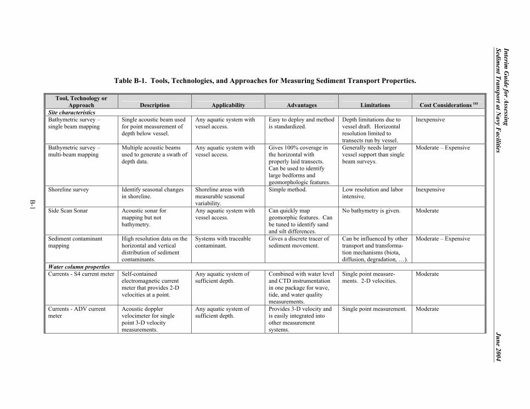
B-1
Interim G
uide for Assessing
Sediment Transport at N
avy Facilities
June 2004
Table B-1. Tools, Technologies, and Approaches for Measuring Sediment Transport Properties.
Tool, Technology or Approach Description Applicability Advantages Limitations Cost Considerations (a)
Site characteristics Bathymetric survey – single beam mapping
Single acoustic beam used for point measurement of depth below vessel.
Any aquatic system with vessel access.
Easy to deploy and method is standardized.
Depth limitations due to vessel draft. Horizontal resolution limited to transects run by vessel.
Inexpensive
Bathymetric survey – multi-beam mapping
Multiple acoustic beams used to generate a swath of depth data.
Any aquatic system with vessel access.
Gives 100% coverage in the horizontal with properly laid transects. Can be used to identify large bedforms and geomorphologic features.
Generally needs larger vessel support than single beam surveys.
Moderate – Expensive
Shoreline survey Identify seasonal changes in shoreline.
Shoreline areas with measurable seasonal variability.
Simple method. Low resolution and labor intensive.
Inexpensive
Side Scan Sonar Acoustic sonar for mapping but not bathymetry.
Any aquatic system with vessel access.
Can quickly map geomorphic features. Can be tuned to identify sand and silt differences.
No bathymetry is given. Moderate
Sediment contaminant mapping
High resolution data on the horizontal and vertical distribution of sediment contaminants.
Systems with traceable contaminant.
Gives a discrete tracer of sediment movement.
Can be influenced by other transport and transforma-tion mechanisms (biota, diffusion, degradation, …).
Moderate – Expensive
Water column properties Currents - S4 current meter Self-contained
electromagnetic current meter that provides 2-D velocities at a point.
Any aquatic system of sufficient depth.
Combined with water level and CTD instrumentation in one package for wave, tide, and water quality measurements.
Single point measure-ments. 2-D velocities.
Moderate
Currents - ADV current meter
Acoustic doppler velocimeter for single point 3-D velocity measurements.
Any aquatic system of sufficient depth.
Provides 3-D velocity and is easily integrated into other measurement systems.
Single point measurement. Moderate

B-2
Interim G
uide for Assessing
Sediment Transport at N
avy Facilities
June 2004
Table B-1. Tools, Technologies, and Approaches for Measuring Sediment Transport Properties (continued).
Tool, Technology or Approach Description Applicability Advantages Limitations Cost Considerations (a)
Water column properties (continued) Currents - PC-ADP current meter
Pulse coherent – acoustic doppler profiler provides 3-D velocity profile near the sediment bed.
Any aquatic system of sufficient depth.
High-resolution velocity profile near the bed allows for wave and current shear stresses on the sediment bed to be directly measured.
Only provides near-bed measurements which can limit description of stratified systems.
Moderate – Expensive
Currents - upward looking ADCP current meter
Subsurface-deployed acoustic profiler provides 2-D velocity profiles through the entire water column.
Any aquatic system of sufficient depth.
Standardized system provides wave and current information. Can be tailored to specific water depths. Data can be used to determine shear stress. Can also be used to deter-mine suspended sediments.
Only single point profile. Must be carefully cali-brated for suspended sediments.
Moderate - Expensive
Currents - boat mounted downward looking ADCP current meter
Vessel-deployed acoustic profiler provides downward looking 2-D current profiles.
Any aquatic system of sufficient depth.
Standardized system provides current information at a point or along transects. Can be used to determine shear stress and suspended solids.
Must be relatively calm water. Only provides relatively short-term snapshot during time of deployment. Must be carefully calibrated for suspended sediments.
Moderate - Expensive
Currents - mechanical current meter
Measures velocity and direction of currents.
Any aquatic system of sufficient depth.
Very simple to deploy. Low accuracy and only provides single data point. In situ deployments must be short term due to fouling.
Inexpensive
Waves and tides - pressure sensors to measure wave and tide height
Measures subsurface pressure to determine water surface variations due to waves and tides.
Any aquatic system of sufficient depth.
Easily deployable and calibrated. Applicable to any type of aquatic system.
Higher memory sensor required for wave measurements. Only provides single point measurement.
Inexpensive

B-3
Interim G
uide for Assessing
Sediment Transport at N
avy Facilities
June 2004
Table B-1. Tools, Technologies, and Approaches for Measuring Sediment Transport Properties (continued).
Tool, Technology or Approach Description Applicability Advantages Limitations Cost Considerations (a)
Water column properties (continued) Salinity - conductivity meter
Measurement of salinity. Any aquatic system of sufficient depth.
Easily deployable and calibrated.
Single point measurement. Inexpensive
Temperature - temperature recorder
Measurement of temperature.
Any aquatic system of sufficient depth.
Easily deployable and calibrated.
Single point measurement. Inexpensive
Suspended sediment concentrations - OBS
Uses optical backscatter techniques to determine suspended sediment concentrations.
Any aquatic system of sufficient depth.
Easily deployable and integrated into other systems. Tunable to be very accurate in specific concentration ranges. Good for very large sediment concentrations.
Single point measurement that is only valid for a specific concentration range. Degradation of data quality due to biofouling over time. Must be calibrated to TSS.
Inexpensive – Moderate
Suspended sediment concentrations - transmissometer
Uses an optical measure of light transmission to determine suspended sediment concentrations.
Any aquatic system of sufficient depth.
Easily deployable and integratable into other systems. Very good in low suspended sediment concentrations.
Single point measurement. Not as durable as other systems. Not good for heavy sediment loads. Must be calibrated to TSS.
Inexpensive - Moderate
Suspended sediment concentrations - LISST 100
Optical measurement of light transmission to determine suspended sediment concentrations and particle size.
Any aquatic system of sufficient depth.
Easily deployable and integrated into other systems. Tunable to be accurate for a specific range of particle sizes and concentrations. Strong Navy support.
Generally needs trained technician to calibrate. Single point measurement that is only valid for a specific concentration range.
Expensive
Suspended sediment concentrations - laboratory determination of TSS
Discrete sample filtered and weighed in laboratory to determine total suspended solids concentration.
Any aquatic system. Generally required for calibration of any other instrumentation. Can be determined for any system at any time. Standardized method available in all aquatic laboratories.
Provides only discrete single point measurement.
Inexpensive

B-4
Interim G
uide for Assessing
Sediment Transport at N
avy Facilities
June 2004
Table B-1. Tools, Technologies, and Approaches for Measuring Sediment Transport Properties (continued).
Tool, Technology or Approach Description Applicability Advantages Limitations Cost Considerations (a)
Sediment bed properties Sediment properties - particle (grain) size distri-bution by sieve analysis
Physical determination of particle size distribution by ASTM D244.
All sediment systems. Standardized method. Labor-intensive and low resolution distributions. Large quantities of sediment required.
Moderate
Sediment properties - particle (grain) size distribution by laser diffraction analysis
Optical determination of particle size by laser scattering properties.
All sediment systems with particle sizes up to 3,000 µm.
Provides very high resolu-tion distributions down to 1 µm. Small quantities required so may be subsampled from other cores.
Non-standard technique. Moderate
Sediment properties - water content/bulk density
Wet and dry weighing of sediments to determine bulk density.
All sediment systems. Standardized measurement required for most sediment transport analyses.
Point measurement. Inexpensive
Sediment properties - total organic carbon
Percentage determination by mass of the total organic carbon present in sediments.
All sediment systems. Can be used for contaminant transport calculations as well.
Point measurement. Moderate
Stratigraphy - sediment core logging
Geologic description of sediment cores to identify sediment types and map stratigraphy.
All sedimentary systems where changes in sediment types exist.
Can be used to identify erosion/deposition patterns. Provides ground truth for remote systems. Provides a core that can be subsampled for other purposes.
Disturbs collected core. Relies on generally quali-tative description of sedi-ments. Labor-intensive.
Inexpensive – Moderate
Stratigraphy - sub-bottom profiling
Establishes sediment stratigraphy and density.
All aquatic systems with vessel access that have distinct sediment differences.
Tunable to specific sediment environments. Gives large area coverage and high resolution description of sediment distribution.
Must be ground-truthed. Low penetration in sandy environments. Presence of gas in fine sediments can invalidate results.
Moderate – Expensive
Sediment stability - shaker/annular flume
Establishes critical shear stress and resuspension potential for surficial cohesive sediments.
Any soft sediment systems. Easily deployable and quick processing of cores. Provides core for epi-benthic characterization.
Only provides surficial information.
Moderate

B-5
Interim G
uide for Assessing
Sediment Transport at N
avy Facilities
June 2004
Table B-1. Tools, Technologies, and Approaches for Measuring Sediment Transport Properties (continued).
Tool, Technology or Approach Description Applicability Advantages Limitations Cost Considerations (a)
Sediment bed properties (continued) Sediment stability - Sedflume
Measures critical shear stress sediment erosion profiles with depth for cohesive sediments.
Any soft sediment systems. Provides a direct measure of sediment erosion and critical shear stress. Provides quantitative and qualitative characteriza-tions of sediments and benthic communities with depths up to 1 m.
Labor intensive and limited area coverage.
Moderate – Expensive
Sediment accumulation rate - radioisotope profiles (Pb-210, Cs-137)
Sedimentation rate, sediment mixing profile and rate.
Best suited for fine-grained depositional sites where the sediment column is undisturbed.
Best method available for estimating sediment accumulation rate over time scales of interest.
Accuracy depends on the validity of the assumptions inherent in the method. Method is ineffective for dating if significant post-depositional disturbance has occurred.
Inexpensive - Moderate
Sediment accumulation rate - sediment traps
Assess quantity and quality of sediment settling on the sediment bed.
Any aquatic system of sufficient depth.
Provides in situ measure of sediments settling to bed. No support required during long-term deployments.
No time series data without retrieval and redeploy-ment. No standardized trap design methodology.
Inexpensive - Moderate
Sediment accumulation rate - erosion pin/pole survey
Determines long-term erosion/sedimentation patterns.
Any sediment system. Easily deployable. Easy to obtain measurements.
Measurements at discrete intervals only. Large changes in bed height can be biased by presence of pole and/or pole movement.
Inexpensive
Bioturbation - qualitative benthic survey
Visual inspection of epibenthic (surficial) communities.
All aquatic systems. Quick and efficient method for describing epibenthic communities. Large area coverage easily possible.
Surficial communities are the only ones covered. Not a quantitative measurement.
Moderate
Bioturbation - quantitative benthic survey
Provides an accurate count of epibenthic and infaunal communities.
Systems with observed biotic activity.
Quantitative description of community structure. Can be used to define bioturbation rates and depths throughout a system.
Labor intensive and relies heavily on local expertise of personnel conducting survey.
Expensive

B-6
Interim G
uide for Assessing
Sediment Transport at N
avy Facilities
June 2004
Table B-1. Tools, Technologies, and Approaches for Measuring Sediment Transport Properties (continued).
Tool, Technology or Approach Description Applicability Advantages Limitations Cost Considerations (a)
Sediment bed properties (continued) Bioturbation - sediment profile imaging
Camera is inserted into the sediments to photograph cross-section of sediment and biotic activity.
Any sedimentary system with vessel access.
Remotely deployed technology. High resolution photography of sediment cross-section. Can provide measure of bioturbation.
Only provides 15 cm of depth. Large vessel requirements for deployment. Relies heavily on local expertise of personnel for the determination of bioturbation.
Moderate
Bioturbation - push cores: visual description and high resolution photography
Clear cores pushed into sediments are collected and photographed.
Any sedimentary system. Provides cores on the order of 1 m depth in soft sediment systems. Cores can be used for other analysis. Simple equipment requirements.
Labor intensive and techniques must be modified for deeper (>10 m) waters.
Inexpensive – Moderate
Bioturbation – radioisotope profiles (Th-234, Be-7)
Depth to which short-lived isotopes are found in sediment bed can provide information about short-term mixing rates.
Any sedimentary system. Allows characterization of the surficial, rapidly mixed zone.
Data should be collected and interpreted by a technical expert.
Inexpensive – Moderate
Bioturbation – oxidation-reduction profile measurements
Semi-quantitative measurement of redox potential discontinuity.
Any sedimentary system. Real time, in situ determination of redox discontinuity
Only provides relative changes in redox potential – not absolute measurements
Inexpensive
(a) All costs are relative to other devices in same category.