Interior Point Methods for Large Scale Optimizationbluebox.ippt.pan.pl/.../JGondzioIPPT2019.pdf · Interior Point Methods for Optimization J. Gondzio, Interior Point Methods 25 Years

J. Gondzio IPMs and Engineering Applications

School of Mathematics

TH

E

U N I V E R S

I TY

OF

ED I N B U

RG

H

Interior Point Methods

for Large Scale Optimization

Jacek [email protected]

http://www.maths.ed.ac.uk/~gondzio

IPPT PAN, Warsaw, 4 November 2019 1


Outline• Interior Point Methods for Optimization

– log barrier, first-order conditions, Newton method– linear, quadratic, semidefinite programming, etc.– IPMs are well suited to large scale optimization

• Sparse Approximations: Signal/Image Processing– Inverse problems

→ ℓ1-regularized least squares– Machine Learning (and Big Data)

• Plastic Truss Layout Optimization– Ground structures

→ linear programming formulation– Stability constraints

→ semidefinite programming formulation– Geometry optimization

• Final Remarks



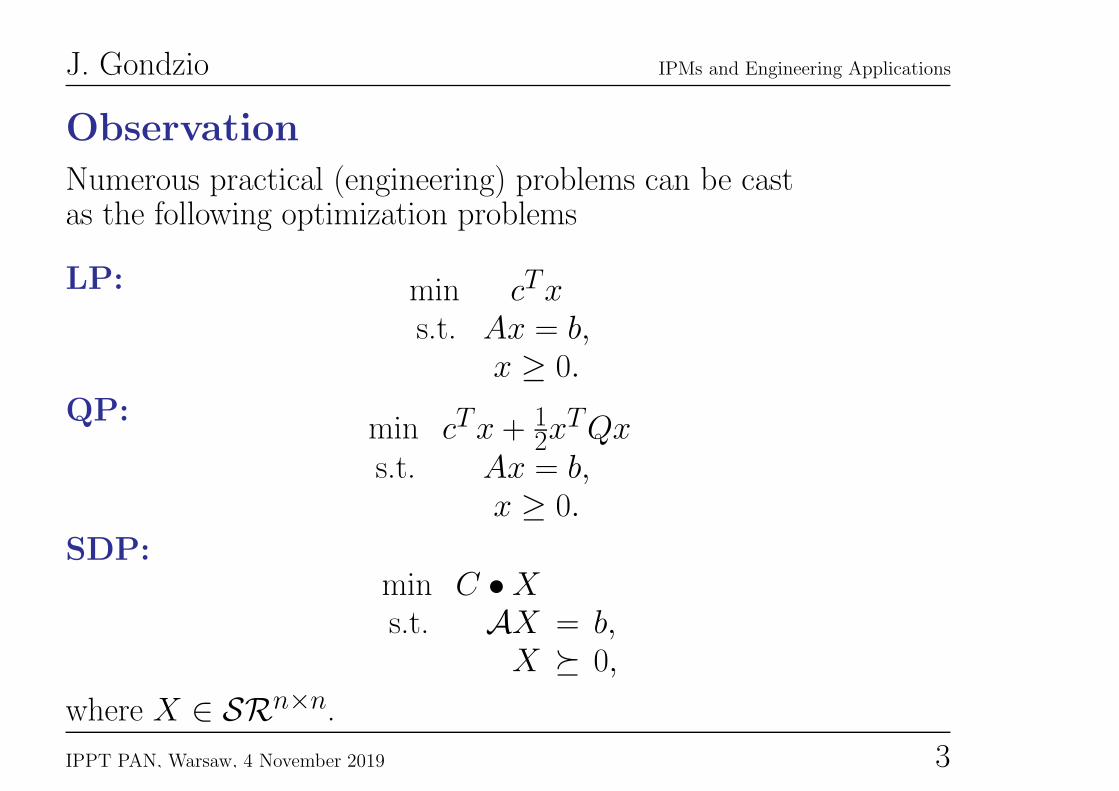
ObservationNumerous practical (engineering) problems can be castas the following optimization problems

LP: min cTxs.t. Ax = b,

x ≥ 0.

QP:min cTx + 1

2xTQx

s.t. Ax = b,x ≥ 0.

SDP:min C •Xs.t. AX = b,

X � 0,

where X ∈ SRn×n.



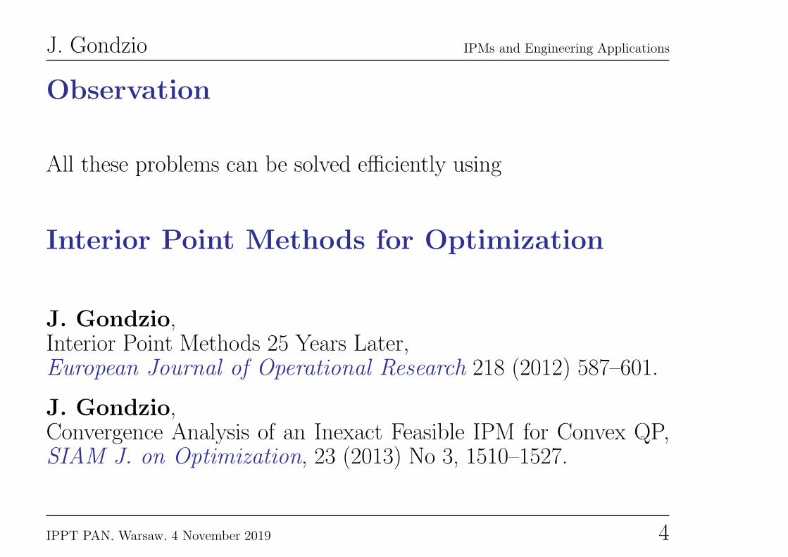
Observation

All these problems can be solved efficiently using

Interior Point Methods for Optimization

J. Gondzio,Interior Point Methods 25 Years Later,European Journal of Operational Research 218 (2012) 587–601.

J. Gondzio,Convergence Analysis of an Inexact Feasible IPM for Convex QP,SIAM J. on Optimization, 23 (2013) No 3, 1510–1527.



Interior Point Methods

Shocking mathematical concept: A step against commonsense and many centuries of mathematical practice:

“nonlinearize” the linear problemTake linear optimization problemand add nonlinear function to the objective.

Mathematical “elements” of the IPM

What do we need to derive the IPM?

• duality theory:Lagrangian function;first order optimality conditions.

• logarithmic barriers.• Newton method.



Primal-Dual Pair of Linear Programs

Primal Dual

min cTx max bTys.t. Ax = b, s.t. ATy + s = c,

x ≥ 0; s ≥ 0.

Lagrangian

L(x, y) = cTx− yT (Ax− b)− sTx.

Optimality Conditions

Ax = b,

ATy + s = c,XSe = 0, ( i.e., xj · sj = 0 ∀j),

(x, s) ≥ 0,

X=diag{x1, · · ·, xn}, S=diag{s1, · · ·, sn}, e = (1, · · ·, 1)∈Rn.



Logarithmic barrier

− ln xj“replaces” the inequality

xj ≥ 0 .

x

−ln x

1

Observe that

min e−∑nj=1 ln xj ⇐⇒ max

n∏

j=1

xj

The minimization of−∑nj=1 ln xj is equivalent to the maximization

of the product of distances from all hyperplanes defining the positiveorthant: it prevents all xj from approaching zero.



Logarithmic barrier

Replace the primal LP

min cTxs.t. Ax = b,

x ≥ 0,

with the primal barrier program

min cTx− µn∑

j=1ln xj

s.t. Ax = b.

Lagrangian: L(x, y, µ) = cTx− yT (Ax− b)− µn∑

j=1

lnxj.



Conditions for a stationary point of the Lagrangian

∇xL(x, y, µ) = c− ATy − µX−1e = 0∇yL(x, y, µ) = Ax− b = 0,

where X−1 = diag{x−11 , x−1

2 , · · · , x−1n }.

Let us denote

s = µX−1e, i.e. XSe = µe.

The First Order Optimality Conditions are:

Ax = b,ATy + s = c,

XSe = µe,(x, s) > 0.



Apply Newton Method to the FOC

The first order optimality conditions for the barrier problem form alarge system of nonlinear equations

f (x, y, s) = 0,

where f : R2n+m 7→ R2n+m is a mapping defined as follows:

f (x, y, s) =

Ax − bATy + s − c

XSe − µe

.

Actually, the first two terms of it are linear; only the last one,corresponding to the complementarity condition, is nonlinear.



Interior-Point FrameworkThe logarithmic barrier

− ln xj

“replaces” the inequality xj ≥ 0.

We derive the first order optimality conditions for the primalbarrier problem:

Ax = b,ATy + s = c,

XSe = µe,

and apply Newton method to solve this system of (nonlinear)equations.

Actually, we fix the barrier parameter µ and make only one (damped)Newton step towards the solution of FOC. We do not solve the FOCexactly. Instead, we immediately reduce the barrier parameter µ (toensure progress towards optimality) and repeat the process.



Self-concordant Barrier

Def: Let C ∈ Rn be an open nonempty convex set.

Let f : C 7→ R be a 3 times continuously diff’able convex function.

A function f is called self-concordant if there exists a constant

p > 0 such that

|∇3f(x)[h, h, h]| ≤ 2p−1/2(∇2f(x)[h, h])3/2,

∀x ∈ C, ∀h : x+h ∈ C. (We then say that f is p-self-concordant).

Note that a self-concordant function is always well approximated bythe quadratic model because the error of such an approximation canbe bounded by the 3/2 power of ∇2f (x)[h, h].

Lemma The barrier function − log x is self-concordant on R+.

Nesterov and Nemirovskii,Interior Point Polynomial Algorithms in Convex Programming:Theory and Applications, SIAM, 1994.



From LP via QP to NLP, SOCP and SDPFor the quadratic cone

Kq = {(x, t) : x ∈ Rn−1, t ∈ R, t2 ≥ ‖x‖2, t ≥ 0},

define the logarithmic barrier function, f : Rn 7→ R

f (x, t) =

{

− ln(t2 − ‖x‖2) if ‖x‖ < t+∞ otherwise.

For the cone SRn×n+ of positive definite matrices,

define the logarithmic barrier function, f : SRn×n+ 7→ R

f (X) =

{

− ln detX if X ≻ 0+∞ otherwise.

LP: Replace x ≥ 0 with −µ∑nj=1 ln xj.

SDP: Replace X � 0 with −µ∑nj=1 lnλj = −µ ln(

∏nj=1 λj).



Interior Point Methods:• Unified view of optimization→ from LP via QP to NLP, SOCP and SDP

• Predictable behaviour→ small number of iterations

• Unequalled efficiency– competitive for small problems (n ≤ 106)– beyond competition for large problems (n ≥ 106)

Problem of size 109 solved in 2005.

Object-Oriented Parallel IPM Solver (OOPS):http://www.maths.ed.ac.uk/~gondzio/parallel/solver.html

Gondzio and Grothey, Parallel IPM solver for structured QPs:application to financial planning problems,Annals of Operations Research 152 (2007) 319-339.



Overarching Feature of IPMs

They possess an unequalled ability to identifythe “essential subspace”

in which the optimal solution is hidden.



Machine Learning/Big Data

Sparse Approximation

• Machine Learning: Classification with SVMs

• Statistics: Estimate x from observations

• Wavelet-based signal/image reconst. & restoration

• Compressed Sensing (Signal Processing)

All such problems lead to the same dense, possibly very large QP.



Binary Classification

min τ‖x‖1+m∑

i=1log(1+e−bix

Tai) min τ‖x‖22+m∑

i=1log(1+e−bix

Tai)



ℓ1-regularization

minx

τ‖x‖1 + φ(x).

think of LASSO:

minx

f (x) = τ‖x‖1 + ‖Ax− b‖22

Unconstrained optimization ⇒ easy

Serious Issue: nondifferentiability of ‖.‖1

Two possible tricks:

• Splitting x = u− v with u, v ≥ 0

• Smoothing with pseudo-Huber approximation

replaces ‖x‖1 with ψµ(x) =∑ni=1(

√

µ2 + x2i − µ)



Huber:



Continuation

Embed inexact Newton Meth into a homotopy approach:

• Inequalities u ≥ 0, v ≥ 0 −→ use IPM

replace z ≥ 0 with −µ logz and drive µ to zero.

• pseudo-Huber regression −→ use continuation

replace |xi| with µ(

√

1+x2iµ2

−1) and drive µ to zero.

Questions:• Theory?

• Practice?



Compressed Sensing and Continuation

Replace minx

f (x) = τ‖W ∗x‖1 +1

2‖Ax− b‖22, −→ xτ

with minx

fµ(x) = τψµ(W∗x) +

1

2‖Ax− b‖22, −→ xτ,µ

Solve approximately a family of problems for a (short) decreasingsequence of µ’s: µ0 > µ1 > µ2 · · ·

Theorem (Brief description)

There exists a µ such that ∀µ ≤ µ the difference of the two solutionssatisfies

‖xτ,µ − xτ‖2 = O(µ1/2) ∀ τ, µ

Primal-Dual Newton Conjugate Gradient Method:

Fountoulakis and Gondzio, A Second-order Method for Strongly Convex ℓ1-regularization Problems,Mathematical Programming, 156 (2016) 189–219.

Dassios, Fountoulakis and Gondzio, A Preconditioner for a Primal-Dual Newton Conjugate Gradient

Method for Compressed Sensing Problems, SIAM J on Scientific Computing, 37 (2015) A2783–A2812.



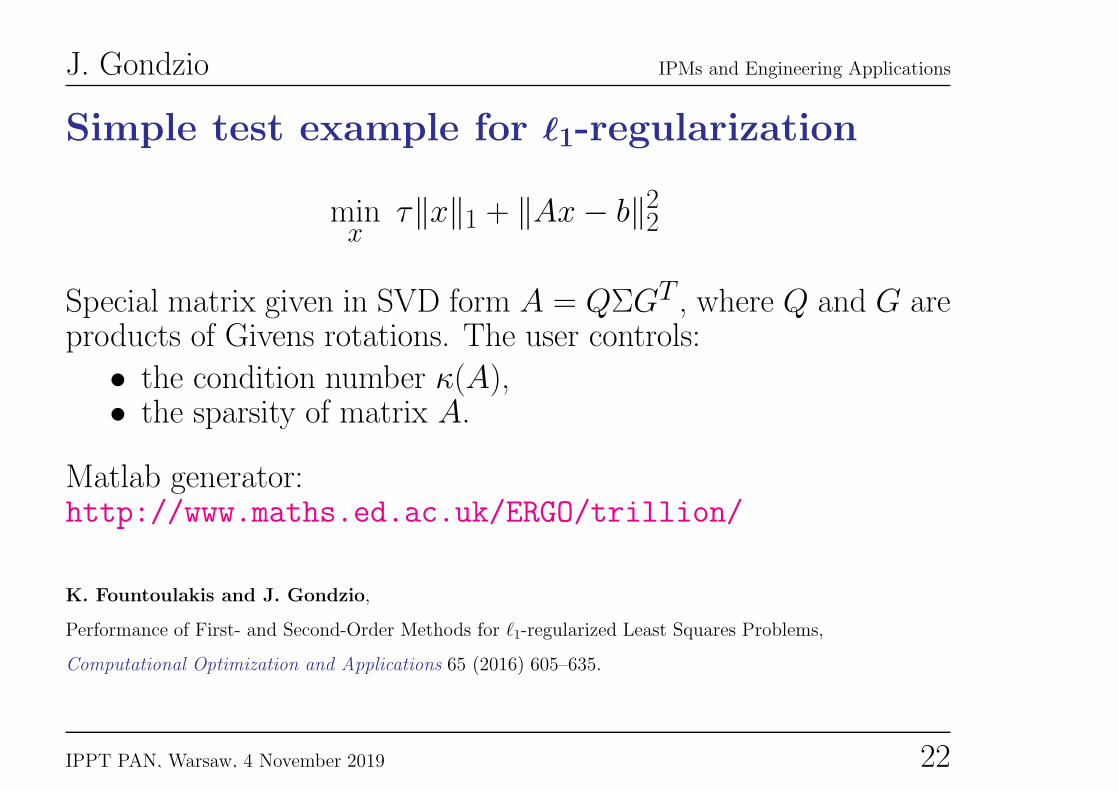
Simple test example for ℓ1-regularization

minx

τ‖x‖1 + ‖Ax− b‖22

Special matrix given in SVD form A = QΣGT , where Q and G areproducts of Givens rotations. The user controls:

• the condition number κ(A),• the sparsity of matrix A.

Matlab generator:http://www.maths.ed.ac.uk/ERGO/trillion/

K. Fountoulakis and J. Gondzio,

Performance of First- and Second-Order Methods for ℓ1-regularized Least Squares Problems,

Computational Optimization and Applications 65 (2016) 605–635.



Let us go big: a trillion (240) variables

n (billions) Processors Memory (TB) time (s)1 64 0.192 19234 256 0.768 196816 1024 3.072 198664 4096 12.288 1970256 16384 49.152 1990

1,024 65536 196.608 2006

ARCHER (ranked 25 on top500.com, 11 March 2015)

Linpack Performance (Rmax) 1,642.54 TFlop/sTheoretical Peak (Rpeak) 2,550.53 TFlop/s



Optimization of truss structures

Potential applications:

the design of

• bridges

• exoskeleton of tall buildings

• large span roof structures, etc



Optimization of truss structures

Given the following:

• d nodes,

• n bars and their lengths,

• external forces f ,

• boundary conditions (some fixed nodes),

find the lightest truss structure that can support the applied loads.

(a) Design domain, boundary (b) Optimal designconditions, and loads



The truss problem: plastic design formulation

minimizea,qℓ

lTa

subject to Bqℓ = fℓ, ℓ = 1, · · · , nL− σ−a ≤ qℓ ≤ σ+a, ℓ = 1, · · · , nLa ≥ 0

• nL number of load cases,

• l ∈ Rn is a vector of bar lengths,

• a ∈ Rn is a vector of bar cross-sectional areas,

• fℓ ∈ Rm is a vector of applied load forces,

• qℓ ∈ Rn are axial forces in members,

• σ− > 0 and σ+ > 0 are the the material’s yieldstresses in compression and tension,

• B ∈ Rm×n nodal equilibrium matrix.

This is a large-scale LP.For d nodes, N -dim problem:

m = Nd, n =d(d−1)

2hence n≫ m.

A challenge for optimization methods!



Difficult optimization problem

For fine grid, the resulting linear programming problem may be verylarge (m is in millions and n easily goes to billions).

Design a specialized IPM for it• n≫ m→ use column generation technique

• a sequence of ‘similar’ problems to be solved→ use warm-starting ability of IPM

• difficult linear systems to solve→ exploit special structure of the problem, i.e.,use appropriately preconditioned Krylov-subspace method



Numerical results

2D 3D# of potential bars in the original problem 85,027,320 163,452,240# of primal vars in the original problem 340,109,280 653,808,960# of constraints in the original problem 85,053,399 16,350,647# of member adding iterations 9 8# of bars in the largest LP solved 201,796 498,058# of primal vars in the largest LP solved 807,184 1,992,232# of constraints in the largest LP solved 227,875 552,289Total CPU[s] (applying) column generation 311 1220



Stability constraints

Design domains, bc, and loads. Without stability considerations. With stability considerations.

• Without stability considerations:– A slender bar lacks any kind of support or bracing (?)– A bridge includes only independent planar trusses (?)

• With stability considerations:– The bar has bracing.– The planar trusses in the bridge are connected.

M. Stingl, On the solution of nonlinear semidefinite programs byaugmented Lagrangian method, PhD thesis 2006,IAM II, Friedrich-Alexander U. of Erlangen–Nuremberg.



Stability constraintsThe stiffness matrix K(a) is given by

K(a) =

n∑

j=1

ajKj, with Kj =E

ljγjγ

Tj (E = Young’s modulus)

and the geometry stiffness matrix G(q) is given by

G(q) =n∑

j=1

qjGj, with Gj =1

lj(δjδ

Tj + ηjη

Tj ),

such that (δj, γj, ηj) are mutually orthogonal (η = 0 for 2D probs).

Global stability constraint:K(a) + τG(q) � 0.

M. Kocvara, On the modelling and solving of the truss designproblem with global stability constraints,Structural and Multidisciplinary Optimization 23(2002), 189–203.



The truss problem with stability constraintsWe consider the so-called global stability which is based on linearbuckling. This leads to the following SDP formulation

mina,qℓ,uℓ

lTa

s.t.ajE

ljγTj uℓ = qℓ,j, ∀ℓ,∀j

Bqℓ = fℓ, ∀ℓ

− σ−a ≤ qℓ ≤ σ+a, ∀ℓK(a) + τℓG(qℓ) � 0, ∀ℓa ≥ 0.

Ignore the kinematic compatibility constraintajEljγTj uℓ = qℓ,j.

But control its violation:

minuℓ

maxℓ

∑

j

(ajE

ljγTj uℓ − qℓ,j)

2



Constraints on eigenfrequencyMinimum compliance problem with a constraint on eigenfrequency

mina,uℓ

lTa

s.t. K(a)uℓ = fℓ, ∀ℓ

fTℓ uℓ ≤ c, ∀ℓK(a)− λM (a) � 0,a ≥ 0.

→

mina

lTa

s.t.

[

c fTℓfℓ K(a)

]

� 0, ∀ℓ

K(a)− λM (a) � 0,a ≥ 0.

The three constraints K(a)u = f, K(a) � 0 and fTu ≤ c arereplaced with a (linear) SDP constraint

[

c fT

f K(a)

]

� 0.

M. Kocvara, On the modelling and solving of the truss designproblem with global stability constraints,Structural and Multidisciplinary Optimization 23(2002), 189–203.



Example: The bridge problem

Small-scale problem: 3,240 bars.



Example: The bridge problemLarge-scale problem: 90,100 bars.

A.G. Weldeyesus and J. Gondzio,A specialized primal-dual interior point method for the plastic truss layout optimization,Computational Optimization and Applications, 71(2018) 613–640.

A.G. Weldeyesus, J. Gondzio, L. He, M. Gilbert, P. Shepherd, A. Tyas,

Adaptive solution of truss layout optimization problems with global stability constraints,

Structural and Multidisciplinary Optimization. https://doi.org/10.1007/s00158-019-02312-9



Example (cont’d)



Geometry Optimization

Allow to move nodes

vol = 7.1191 vol = 6.3128



Geometry Optimization: Bridge design

vol = 3.6980vol = 3.1796



Conclusions

• IPMs are well-suited to solving large scaleoptimization problems

– predictable behaviour– high accuracy

• IPMs can be applied in various contexts

Use IPMs in your research!


Documents

Interior Point Methods for Large Scale Optimizationbluebox.ippt.pan.pl/.../JGondzioIPPT2019.pdf · Interior Point Methods for Optimization J. Gondzio, Interior Point Methods 25 Years