Embed Size (px)
Citation preview

INTERMEDIATE (IPC) COURSE
STUDY MATERIAL
PAPER : 3
COST ACCOUNTING AND
FINANCIAL MANAGEMENT Part – 1 : Cost Accounting
MODULE – 1
BOARD OF STUDIES
THE INSTITUTE OF CHARTERED ACCOUNTANTS OF INDIA
© The Institute of Chartered Accountants of India

ii
This Study Material has been prepared by the faculty of the Board of Studies. The objective of
the study material is to provide teaching material to the students to enable them to obtain
knowledge in the subject. In case students need any clarifications or have any suggestions to
make for further improvement of the material contained herein, they may write to the Director
of Studies.
All care has been taken to provide interpretations and discussions in a manner useful for the
students. However, the study material has not been specifically discussed by the Council of
the Institute or any of its Committees and the views expressed herein may not be taken to
necessarily represent the views of the Council or any of its Committees.
Permission of the Institute is essential for reproduction of any portion of this material.
© The Institute of Chartered Accountants of India
All rights reserved. No part of this book may be reproduced, stored in a retrieval system, or
transmitted, in any form, or by any means, electronic, mechanical, photocopying, recording, or
otherwise, without prior permission, in writing, from the publisher.
Revised Edition : April, 2016
Website : www.icai.org
E-mail : [email protected]
Committee/ : Board of Studies
Department
ISBN No. :
Price (All Modules) : `
Published by : The Publication Department on behalf of The Institute of
Chartered Accountants of India, ICAI Bhawan, Post Box No.
7100, Indraprastha Marg, New Delhi 110 002, India.
Printed by :
© The Institute of Chartered Accountants of India

iii
A WORD ABOUT STUDY MATERIAL
The Study Material has been divided into two parts, namely, Study Material dealing with
conceptual theoretical framework; and Practice Manual. The Study Material has been
designed having regard to the needs of home study and distance learning students in mind.
The students are expected to cover the entire syllabus and also do practice on their own while
going through the Practice Manual.
The Study Material deals with the specific conceptual theoretical framework of cost accounting
in detail. The main features of Study Material are as under:
The entire syllabus has been divided into thirteen chapters.
The chapters have been grouped into two modules
Module- 1 consisting of four chapters namely :
Chapter- 1: Basic Concepts
Chapter- 2: Material
Chapter- 3: Labour
Chapter- 4: Overheads
Module- 2 consisting of nine chapters namely:
Chapter- 5: Non-integrated Accounts
Chapter- 6: Job Costing and Batch Costing
Chapter- 7: Contract Costing
Chapter- 8: Operating Costing
Chapter- 9: Process & Operation Costing
Chapter- 10: Joint Products & By Products
Chapter- 11: Standard Costing
Chapter- 12: Marginal Costing
Chapter- 13: Budgets and Budgetary Control
In each chapter, learning objectives have been stated. The learning objectives would
enable you to understand the sequence of various aspects dealt within the chapter before
going into the details so that you know the direction of your studies.
© The Institute of Chartered Accountants of India

iv
In each chapter, the topic has been covered in step by step approach. The text has been
explained, where appropriate, through illustrations and practical problems. You should go
through the chapter carefully ensuring that you understand the topic and then can tackle
the exercises.
Main features of Practice Manual are as under:
Questions bunch with compilation of questions appearing during last examinations also.
Important definitions, equations and formulae have been given before each topic for quick
recapitulation. Students are expected to attempt the questions and then compare it with
the actual answers.
Aims to provide guidance as to the manner of writing an answer in the examination.
Feedback form is given in the Module-1 of the Study Material wherein students are
encouraged to give their feedback/ suggestions.
In this Study Material, formats of Financial Statements (i.e. Balance Sheet, Income
Statements etc) and financial terms used are for illustrative purpose only. For appropriate
format and applicability of various Standards, students are advised to refer the study material
of appropriate subject (s).
Every effort has been made to make the Study Material error free, however if inadvertently any
error is present and found by readers they may send it to us immediately so that it can be
rectified at our end.
In case you need any further clarification/ guidance, you may send your queries at
[email protected]; [email protected] and [email protected].
© The Institute of Chartered Accountants of India
vii
SYLLABUS
PAPER – 3 : COST ACCOUNTING AND FINANCIAL MANAGEMENT
(One paper ─ Three hours – 100 Marks)
Level of Knowledge: Working knowledge
PART – I : COST ACCOUNTING (50 MARKS)
Objectives:
(a) To understand the basic concepts and processes used to determine product costs,
(b) To be able to interpret cost accounting statements,
(c) To be able to analyse and evaluate information for cost ascertainment, planning, control
and decision making, and
(d) To be able to solve simple cases.
Contents
1. Introduction to Cost Accounting
(a) Objectives and scope of Cost Accounting
(b) Cost centres and Cost units
(c) Cost classification for stock valuation, Profit measurement, Decision making and
control
(d) Coding systems
(e) Elements of Cost
(f) Cost behaviour pattern, Separating the components of semi-variable costs
(g) Installation of a Costing system
(h) Relationship of Cost Accounting, Financial Accounting, Management Accounting
and Financial Management.
2. Cost Ascertainment
(a) Material Cost
(i) Procurement procedures— Store procedures and documentation in respect of
receipts and issue of stock, Stock verification (ii)Inventory control —
© The Institute of Chartered Accountants of India

viii
Techniques of fixing of minimum, maximum and reorder levels, Economic
Order Quantity, ABC classification; Stocktaking and perpetual inventory
(iii) Inventory accounting
(iv) Consumption — Identification with products of cost centres, Basis for
consumption entries in financial accounts, Monitoring consumption.
(b) Employee Cost
(i) Attendance and payroll procedures, Overview of statutory requirements,
Overtime, Idle time and Incentives
(ii) Labour turnover
(iii) Utilisation of labour, Direct and indirect labour, Charging of labour cost,
Identifying labour hours with work orders or batches or capital jobs
(iv) Efficiency rating procedures
(v) Remuneration systems and incentive schemes.
(c) Direct Expenses
Sub-contracting — Control on material movements, Identification with the main
product or service.
(d) Overheads
(i) Functional analysis — Factory, Administration, Selling, Distribution, Research
and Development Behavioural analysis — Fixed, Variable, Semi variable and
Step cost
(ii) Factory Overheads — Primary distribution and secondary distribution, Criteria
for choosing suitable basis for allotment, Capacity cost adjustments, Fixed
absorption rates for absorbing overheads to products or services
(iii) Administration overheads — Method of allocation to cost centres or products
(iv) Selling and distribution overheads — Analysis and absorption of the expenses
in products/customers, impact of marketing strategies, Cost effectiveness of
various methods of sales promotion.
3. Cost Book-keeping
Cost Ledgers—Non-integrated accounts, Integrated accounts, Reconciliation of cost and
financial accounts.
© The Institute of Chartered Accountants of India

ix
4. Costing Systems
(a) Job Costing
Job cost cards and databases, Collecting direct costs of each job, Attributing
overhead costs to jobs, Applications of job costing.
(b) Batch Costing
(c) Contract Costing
Progress payments, Retention money, Escalation clause, Contract accounts,
Accounting for material, Accounting for plant used in a contract, Contract profit and
Balance sheet entries.
(d) Process Costing
Double entry book keeping, Process loss, Abnormal gains and losses, Equivalent
units, Inter-process profit, Joint products and by products.
(e) Operating Costing System
5. Introduction to Marginal Costing
Marginal costing compared with absorption costing, Contribution, Breakeven analysis
and profit volume graph.
6. Introduction to Standard Costing
Various types of standards, Setting of standards, Basic concepts of material and Labour
standards and variance analysis.
7. Budget and Budgetary Control
The budget manual, preparation and monitoring procedures, budget variances, flexible
budget, preparation of functional budget for operating and non operating functions, cash
budget, master budget, principal budget factors.
© The Institute of Chartered Accountants of India

x
STUDY PLAN – KEY TO EFFECTIVE LEARNING
Introduction
Cost Accounting and Financial Management is a subject which consists of two parts i.e. Cost
accounting and Financial Management. The Cost Accounting part deals with basic concepts of
Cost Accounting, elements of Cost, various methods of Costing and application of costing
techniques. The basic objective of Cost Accounting part is as follows:
(a) To understand the basic concepts and processes used to determine product costs,
(b) To be able to interpret cost accounting statements,
(c) To be able to analyse and evaluate information for cost ascertainment, planning, control
and decision making, and
(d) To be able to solve simple cases.
Outline of the Syllabus
The entire syllabus of the Cost Accounting part has been divided into thirteen chapters. The
topics covered under these chapters are
1. Basic Concepts, 2.Material, 3.Labour, 4.Overheads, 5.Non Integrated Accounts, 6. Job
Costing & Batch Costing 7. Contract Costing 8. Operating Costing 9. Process & Operation
Costing 10. Joint products & By Products 11. Standard Costing 12. Marginal costing 13.
Budgets and Budgetary Control.
Chapter Specific
In the first chapter ‘Basic Concepts’, overview of all the concepts of Cost Accounting
needs to be understood. The major parts which need to understand are definitions and
different terminologies used in Cost Accounting and the context in which these are
normally used. You are required to understand the objectives and importance of Cost
Accounting system and its installation in industry, relation between Cost Accounting with
other fields of study and its synchronisation with other related department/ stake holders
to assist the management of the Organisation. Classification of cost, various elements
and components of cost and various costing methods used in different industries need to
be studied carefully. Theoretical questions are generally asked from this chapter almost
in every examination. To answer these questions conceptual clarity and visualisation of
practical life examples are necessary.
The second chapter ‘Material’ is very important for the students. Students shall
understand the concept, need and importance of materials in production system, various
procedures involved in procuring, storing and issuing of material. You must know the
© The Institute of Chartered Accountants of India

xi
treatment of excess/ shortage of stores and valuation of store to be received, issued &
stock at hand. Components which should form part of value of material should be
understood; you may refer illustrations given in the Study Material. Generally problems
on EOQ are solved using formula but some time instead of using formula answers to the
questions is required to be done in tabular format as shown in the Study Material. You
should also learn to draft format of Store Ledger under different valuation methods and
accounting treatment. Treatment of normal and abnormal loss of materials, waste, scrap,
spoilage and defectives in the Store ledger to be understood to arrive at correct stock
position and its respective value. You should clearly know the differences between
Simple average method and weighted average method of stock valuation. To avoid any
confusion you should read the question carefully and understand the calculation under
two methods of Valuation.
In the third chapter ‘Labour’ students shall learn and understand the need of labour cost
control, methods of attendance and payroll preparation procedures. Treatment of idle
time and overtime both as normal and abnormal should be clearly understood by you.
Students may also refer various illustrations given in the Study material for better and
clear understanding. Labour Turnover is a term which can be heard in almost every
Industry; you should understand what exactly, labour turnover is, reasons for labour
turnover and its impact on an organisation’s productivity directly and on image indirectly.
Be conversed with various methods of computing labour turnover and Incentive plans to
the workers. Students should be acquaintance with of different systems of wage payment
and Incentives through practicing different types of problems. In examination generally
questions are asked to compute Incentives based on a particular incentive plan or make
comparison between two given plans. Students are advised to avoid selective study like
only Rowan or Halsey method of bonus plan.
The fourth chapter ‘Overheads’ in which students shall understand the meaning and
difference between direct cost and indirect cost i.e. overheads. Overheads are generally
associated with more than one department or product line. Overheads are distributed
amongst the concerned departments/ product lines using a basis. Distribution of
overheads is called allocation of overheads or apportionment of overheads or absorption
of overheads. Understanding the meaning and differences among the terms such as
allocation, apportionment and absorption of overhead is important for conceptual clarity.
As stated above overheads are allocated/ apportioned/ absorbed using some basis e.g.
primary distributions are done using labour hours, machine hours, floor area, capacity,
number of staff etc. Students should be versed with treatment of under absorption and
over absorption of overheads through application of supplementary rate while
ascertaining the cost of a particular product or department. You should also learn
different methods of secondary distribution and calculation involved therein. Students
should do thorough practice to avoid computational errors. Some time questions are
related with capacity determination, in this regard students should be familiar with terms
such as Installed/ Rated capacity, normal capacity, practical capacity, actual capacity
etc. Question may be asked to calculate idle capacity and/or cost.
© The Institute of Chartered Accountants of India

xii
In the Fifth chapter ‘Non-Integrated Accounts’ students shall acquainted with both
Integrated and Non-Integrated systems of accounting and different ledgers account to be
opened under the two methods of cost accounting. You should know the reasons for the
differences between profit as per the financial accounting and the cost accounting and
ways to reconcile it. Accounting treatment of over absorption and under absorption of
overheads should be understood.
The sixth, seventh and eighth chapters consist of Job Costing and Batch Costing,
Contract Costing, Operating Costing and Multiple Costing. Here students should
understand the meaning and distinctive features of above mentioned methods of costing
and the accounting procedures to be applied in the above mentioned different methods of
costing. Students shall be conversed with the adjustment of opening and closing stock of
raw material, work in process and finished goods while preparation of Job/ Batch cost
sheet. In Contract Costing profit from the contract is recognised using percentage of
completion method. To arrive at it various factors such as Value of contract, Cost of Work
certified, work uncertified, retention money, cash received should be understood.
Computation of notional profit and estimated profit shall be learned. You should
understand effects of escalation clause both to contractor and contractee and revision of
work certified.
The ninth and tenth chapters consist of Process & Operation Costing and Joint Products
and By Products. Area of application of the above costing methods and accounting
difference among these should be understood. Process Costing method is followed in an
industry where a product passing through various identifiable processes, where output of
one process becomes the input of succeeding process and so on till it reaches its final
shape. Students should be able to identify each process and related cost. Production
being a continuous process where some incomplete (work in process) stock remains a
possibility. To find out accurate cost incurred and output for a given period ‘Statement of
Equivalent Production’ is prepared. Students should be able to calculate equivalent
production for a given period with the use of any methods of inventory valuation.
Students may refer illustrations given in the Study material for practice and clarity. One
most important area of calculation is the treatment of normal loss, abnormal losses/
gains, adjustment for scrap in ascertainment of actual abnormal loss/gain.
Some time more than one final products are obtained from a common process or input.
Students shall know the treatment of joint cost to joint products for stock valuation
purposes. Joint costs are apportioned using various methods such as based on sales
value or based on volume etc. students may refer illustrations given in the Study Material
for clear understanding. Some time questions may be asked on selling price at which a
particular product can be sold or should be sold after further processing. Various
illustrations have been given in the Study materials showing this type of calculations.
Similarly all other methods such as operation costing and costing for By Products should
be understood.
© The Institute of Chartered Accountants of India

xiii
The eleventh chapter is ‘Standard Costing’. First of all students should understand the
meaning of standard cost and what is actual cost. The difference between standard
values with actual value is called variance; Variances are calculated using some rational
and conventional formulas. Formulas and its logical interlinks for finding out variances
should be understood. Mere mugging up of formulas without proper understanding of its
relationship will not going to help, as this chapter is just an introduction, clear
understanding will definitely help students at Final level where numerical are based on
practical situations. Students should also understand the accounting procedures and
disposition of variances. Classification of variances and interrelationship could be
understood from the chart given in the study material. This chapter requires lots of
practice.
‘Marginal Costing’ is the twelfth chapter of Cost Accounting at IPCC level and is one of
the most vital chapter. Basic marginal equations and formulas should be understood.
Students should be able to extract Profit Volume Ratio (P/V Ratio), Break Even Point/
sales, margin of safety, contribution, bifurcation of fixed cost from semi variable cost.
Difference between marginal costing and absorption costing should be understood as
some time you are required to reconcile figures from one method to another. Specimen
Income Statement given in Study material is very helpful for clear understanding of the
differences and treatment.
In thirteenth chapter ‘Budgets and Budgetary Control’, objectives and importance of
budgets and budgetary control, advantages and disadvantages of budgetary control
should be understood. You are also required to learn the difference between various
types of budgets and process of preparation of budgets. Generally preparation of flexible
budget segregation of fixed cost and variable cost is required, so segregation techniques
should be learnt (also discussed in Chapter-1). It is important for the students to
understand inter linkage among different functional budget while answering question on
functional budget. You may refer illustrations given in the Study Material.
Happy Reading and Best Wishes!
© The Institute of Chartered Accountants of India

xiv
© The Institute of Chartered Accountants of India

xv
CONTENTS
MODULE – 1
Chapter 1 – Basic Concepts
Chapter 2 – Material
Chapter 3 – Labour
Chapter 4 – Overheads
MODULE – 2
Chapter 5 – Non Integrated Accounts
Chapter 6 – Job Costing and Batch Costing
Chapter 7 – Contract Costing
Chapter 8 – Operating Costing
Chapter 9 – Process & Operations Costing
Chapter 10 – Joint Products & By Products
Chapter 11 – Standard Costing
Chapter 12 – Marginal Costing
Chapter 13 – Budgets and Budgetary Control
© The Institute of Chartered Accountants of India
xvi
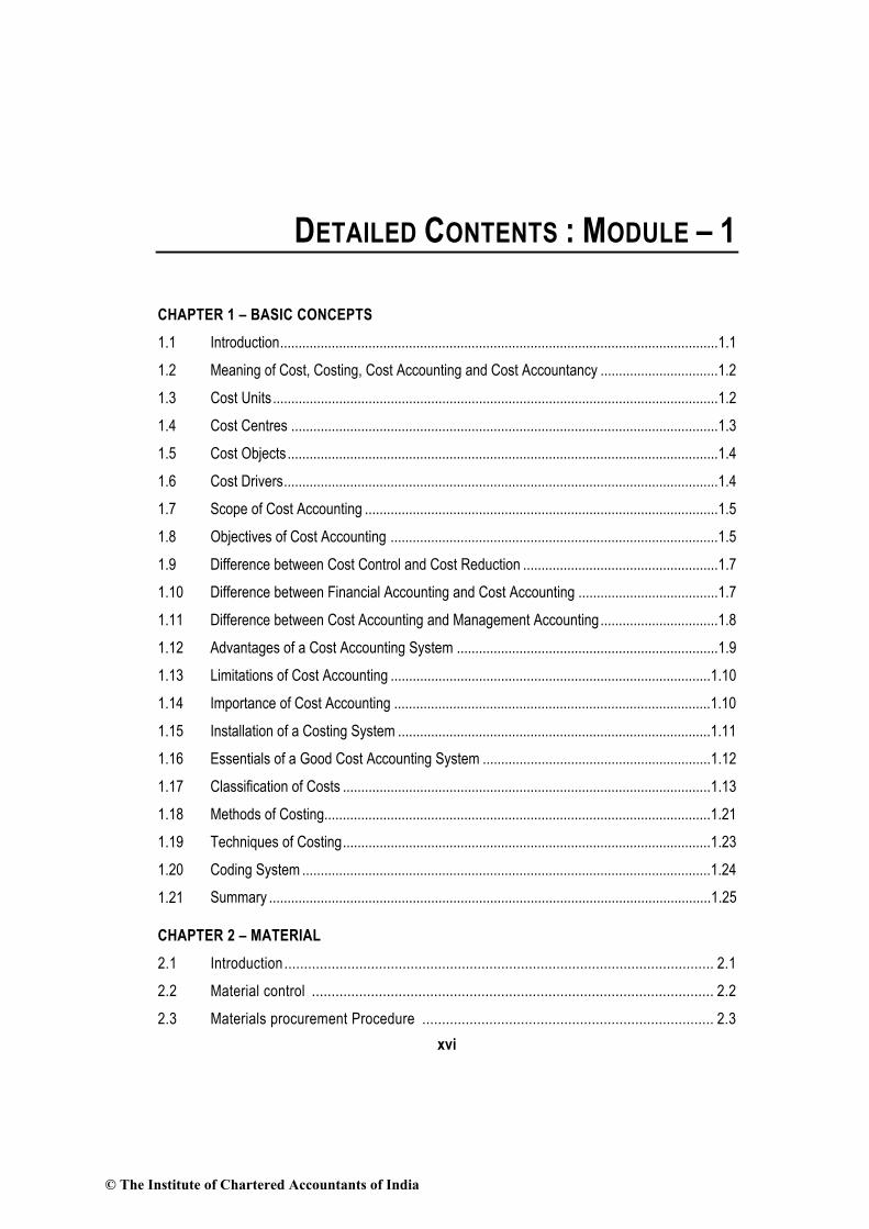
DETAILED CONTENTS : MODULE – 1
CHAPTER 1 – BASIC CONCEPTS
1.1 Introduction ....................................................................................................................... 1.1
1.2 Meaning of Cost, Costing, Cost Accounting and Cost Accountancy ................................ 1.2
1.3 Cost Units ......................................................................................................................... 1.2
1.4 Cost Centres .................................................................................................................... 1.3
1.5 Cost Objects ..................................................................................................................... 1.4
1.6 Cost Drivers ...................................................................................................................... 1.4
1.7 Scope of Cost Accounting ................................................................................................ 1.5
1.8 Objectives of Cost Accounting ......................................................................................... 1.5
1.9 Difference between Cost Control and Cost Reduction ..................................................... 1.7
1.10 Difference between Financial Accounting and Cost Accounting ...................................... 1.7
1.11 Difference between Cost Accounting and Management Accounting ................................ 1.8
1.12 Advantages of a Cost Accounting System ....................................................................... 1.9
1.13 Limitations of Cost Accounting ....................................................................................... 1.10
1.14 Importance of Cost Accounting ...................................................................................... 1.10
1.15 Installation of a Costing System ..................................................................................... 1.11
1.16 Essentials of a Good Cost Accounting System .............................................................. 1.12
1.17 Classification of Costs .................................................................................................... 1.13
1.18 Methods of Costing......................................................................................................... 1.21
1.19 Techniques of Costing .................................................................................................... 1.23
1.20 Coding System ............................................................................................................... 1.24
1.21 Summary ........................................................................................................................ 1.25
CHAPTER 2 – MATERIAL
2.1 Introduction ............................................................................................................. 2.1
2.2 Material control ...................................................................................................... 2.2
2.3 Materials procurement Procedure .......................................................................... 2.3
© The Institute of Chartered Accountants of India

xvii
2.4 Valuation of Material Receipts ............................................................................... 2.11
2.5 Material Storage & Records .................................................................................. 2.14
2.6 Inventory Control .................................................................................................. 2.17
2.7 Material Issue Procedure ...................................................................................... 2.43
2.8 Valuation of Material Issues .................................................................................. 2.45
2.9 Valuation of Returns & Shortages ......................................................................... 2.63
2.10 Selection of Pricing Method................................................................................... 2.63
2.11 Treatment of normal and abnormal loss of materials ............................................. 2.64
2.12 Accounting & Control of Waste, Scrap, Spoilage and Defectives ........................... 2.64
2.13 Consumption of Materials...................................................................................... 2.69
2.14 Summary .............................................................................................................. 2.71
CHAPTER 3 – LABOUR
3.1 Introduction ............................................................................................................. 3.1
3.2 Classification of Labour Cost................................................................................... 3.1
3.3 Labour Cost Control ............................................................................................... 3.2
3.4 Attendance & Payroll procedures ............................................................................ 3.4
3.5 Idle Time ............................................................................................................... 3.12
3.6 Overtime ............................................................................................................... 3.14
3.7 Labour turnover .................................................................................................... 3.21
3.8 Incentive system ................................................................................................... 3.27
3.9 Labour utilisation ................................................................................................... 3.30
3.10 Systems of Wage Payment and Incentives ............................................................ 3.31
3.11 Absorption of Wages ............................................................................................. 3.68
3.12 Efficiency Rating Procedures ................................................................................ 3.74
3.13 Summary .............................................................................................................. 3.76
CHAPTER 4 – OVERHEADS
4.1 Introduction ............................................................................................................. 4.1
4.2 Classification of Overheads..................................................................................... 4.2
4.3 Accounting and Control of Manufacturing Overheads ............................................. 4.5
© The Institute of Chartered Accountants of India

xviii
4.4 Steps for the Distribution of Overheads ................................................................... 4.8
4.5 Methods of Absorbing Overheads to Various Products or Jobs ............................ 4.26
4.6 Types of Overhead Rates ..................................................................................... 4.31
4.7 Treatment of Under-Absorbed and Over-Absorbed Overheads in Cost Accounting ... 4.42
4.8 Accounting and Control of Administrative Overheads ........................................... 4.54
4.9 Accounting and Control of Selling and Distribution Overheads .............................. 4.58
4.10 Concepts Related to Capacity .............................................................................. 4.61
4.11 Treatment of Certain Items in Costing .................................................................. 4.63
4.12 Summary .............................................................................................................. 4.65
© The Institute of Chartered Accountants of India

1 Basic Concepts
Learning Objectives
After studying this chapter you will be able to:
♦ Understand the Cost Accounting System.
♦ Know about the objective and importance of Cost Accounting.
♦ Basic Cost Accounting terminology used in the subject.
♦ Difference and relation between Cost Accounting and Financial Accounting and Management Accounting will become clear.
♦ Understand the process of installation of Cost Accounting system with the key factors to be recognized for the process to take place.
♦ Classify costs into different categories.
♦ Identify different elements and components of costs and
♦ Understand and apply the various methods of costing used in the industry.
♦ The concept of Codes and the process of codification will become clear.
1.1 Introduction
In the seventeenth century in France, the Royal Wallpaper Manufactory had a Cost Accounting
System. Some iron masters and potters in eighteenth century in England too began to produce
Cost Accounting information before the Industrial Revolution. However, the period, 1880 AD –
1925 AD saw the development of complex product designs and the emergence of multi activity
diversified corporations like Du Pont, General Motors etc. It was during this period that scientific
management was developed which led accountants to convert physical standards into cost
standards, the latter being used for variance analysis and control.
During World War I and II the social importance of cost accounting grew with the growth of each
country’s defence expenditure. In the absence of competitive markets for most of the material
required to fight war, the Governments in several countries placed cost-plus contracts under
which the price to be paid was the cost of production plus an agreed rate of profit. The reliance
on cost information by the parties to defence contracts continued after World War II as well.
© The Institute of Chartered Accountants of India

1.2 Cost Accounting
1.2 Meaning of Cost, Costing, Cost Accounting and Cost Accountancy
Term Meaning
Cost
As a noun- The amount of expenditure (actual or notional) incurred
on or attributable to a specified article, product or activity.
As a verb- To ascertain the cost of a specified thing or activity.
Costing
Costing is defined as “the technique and process of ascertaining
costs”.
According to CIMA “An organisation costing system is the foundation
of the internal financial information system for managers. It provides
the information that management needs to plan and control the
organisation’s activities and to make decisions about the future.”
Cost Accounting
Cost Accounting is defined as "the process of accounting for cost
which begins with the recording of income and expenditure or the
bases on which they are calculated and ends with the preparation of
periodical statements and reports for ascertaining and controlling
costs."
Cost Accountancy
Cost Accountancy has been defined as “the application of costing and
cost accounting principles, methods and techniques to the science,
art and practice of cost control and the ascertainment of profitability.
It includes the presentation of information derived there from for the
purpose of managerial decision making.”
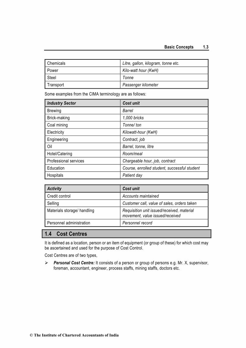
1.3 Cost Units
It is a unit of product, service or time (or combination of these) in relation to which costs may be ascertained or expressed.
We may for instance determine the cost per tonne of steel, per tonne kilometre of a transport service or cost per machine hour. Sometime, a single order or a contract constitutes a cost unit. A batch which consists of a group of identical items and maintains its identity through one or more stages of production may also be considered as a cost unit.
Cost units are usually the units of physical measurement like number, weight, area, volume, length, time and value.
A few typical examples of cost units are given below:
Industry or Product Cost Unit Basis
Automobile Number
Cement Tonne/ per bag etc.
© The Institute of Chartered Accountants of India
Basic Concepts 1.3
Chemicals Litre, gallon, kilogram, tonne etc.
Power Kilo-watt hour (KwH)
Steel Tonne
Transport Passenger kilometer
Some examples from the CIMA terminology are as follows:
Industry Sector Cost unit
Brewing Barrel
Brick-making 1,000 bricks
Coal mining Tonne/ ton
Electricity Kilowatt-hour (KwH)
Engineering Contract, job
Oil Barrel, tonne, litre
Hotel/Catering Room/meal
Professional services Chargeable hour, job, contract
Education Course, enrolled student, successful student
Hospitals Patient day
Activity Cost unit
Credit control Accounts maintained
Selling Customer call, value of sales, orders taken
Materials storage/ handling Requisition unit issued/received, material movement, value issued/received
Personnel administration Personnel record
1.4 Cost Centres
It is defined as a location, person or an item of equipment (or group of these) for which cost may be ascertained and used for the purpose of Cost Control.
Cost Centres are of two types,
Personal Cost Centre: It consists of a person or group of persons e.g. Mr. X, supervisor,
foreman, accountant, engineer, process staffs, mining staffs, doctors etc.
© The Institute of Chartered Accountants of India

1.4 Cost Accounting
Impersonal Cost Centre: It consists of a location or an item of equipment (or group of
these) e.g. Ludhiana branch, boiler house, cooling tower, weighing machine, canteen, and
generator set etc.
Cost Centre in a manufacturing concern:
Two main types of Cost Centres are indicated as below:
Production Cost Centre: It is a cost centre where raw material is handled for conversion
into finished product. Here both direct and indirect expenses are incurred. Machine shops,
welding shops and assembly shops etc. are examples of production Cost Centres.
Service Cost Centre: It is a cost centre which serves as an ancillary unit to a production
cost centre. Payroll processing department, HRD, Power house, gas production shop,
material service centres, plant maintenance centres etc. are examples of service cost
centres.
1.5 Cost Objects
Cost object is anything for which a separate measurement of cost is required. Cost object may be a
product, a service, a project, a customer, a brand category, an activity, a department or a programme
etc.
Examples of Cost Object are:
• Product Smart phone, Tablet computer, SUV Car, Book etc.
• Services An airline flight from Delhi to Mumbai, Concurrent audit assignment, Utility bill payment facility etc.
• Project Metro Rail project of DMRC, Road projects of NHAI etc.
• Activity Quality inspection of materials, Placing of orders etc.
• Process Refinement of crudes in oil refineries, melting of billets or ingots in rolling mills etc.
• Department Production department, Finance & Accounts, Safety etc
1.6 Cost Drivers
A Cost driver is a factor or variable which effect level of cost. Generally it is an activity which is
responsible for cost incurrence. Level of activity or volume of production is the example of a
cost driver. An activity may be an event, task, or unit of work etc.
CIMA Official terminology defines cost driver as “Factor influencing the level of cost. Often used
in the context of ABC to denote the factor which links activity resource consumption to product
outputs, for example the number of purchase orders would be a cost driver for procurement
cost.”
© The Institute of Chartered Accountants of India

Basic Concepts 1.5
Examples of cost drivers are number of machines setting ups, number of purchase orders, hours
spent on product inspection, number of tests performed etc.
1.7 Scope of Cost Accounting
Scope of cost accounting consists of the following functions:
(i) Costing: Costing is the technique and process of ascertaining costs of products or
services. The cost ascertainment procedure is governed by some cost accounting
principles and rules. Generally cost is ascertained using some arithmetical process.
(ii) Cost Accounting: This is a process of accounting for cost which begins with the recording
of expenditure and ends with the preparation of periodical statement and reports for
ascertaining and controlling cost. Cost Accounting is a formal mechanism of cost
ascertainment.
(iii) Cost Analysis: It involves the process of finding out the factors responsible for variance
in actual costs from the budgeted costs and accordingly fixation of responsibility for cost
differences. This also helps in better cost management and strategic decisions.
(iv) Cost Comparisons: Cost accounting also includes comparisons of cost from alternative
courses of action such as use of different technology for production, cost of making
different products and activities, and cost of same product/ service over a period of time.
(v) Cost Control: It involves a detailed examination of each cost in the light of advantage
received from the incurrence of the cost. Thus, we can state that cost is analyzed to know
whether cost is not exceeding its budgeted cost and whether further cost reduction is
possible or not.
(vi) Cost Reports: This is the ultimate function of cost accounting. These reports are primarily
prepared for use by the management at different levels. Cost Reports helps in planning
and control, performance appraisal and managerial decision making.
(vii) Statutory Compliances: Maintaining cost accounting records as per the rules prescribed
by the statute. As per the Companies (Cost Records and Audits) Rules, 2014, Companies
governed by the Companies Act has to maintain cost records relating to utilization of
materials, labour and other items of cost as applicable to the production of goods or
provision of services as provided in the Act and these rules..
1.8 Objectives of Cost Accounting
The main objectives of Cost Accounting are explained as follows:
(i) Ascertainment of Cost: There are two methods of ascertaining costs:
Post Costing: It means analysis of actual information as recorded in financial books. It is
accurate and is useful in the case of “Cost plus contracts” where price is to be determined
finally on the basis of actual cost.
© The Institute of Chartered Accountants of India

1.6 Cost Accounting
Continuous Costing: It aims at collecting information about cost as and when the activity
takes place so that as soon as a job is completed the cost of completion would be known.
This involves careful estimation of overheads. In order to be of any use, costing must be a
continuous process.
Cost ascertained by the above two methods may be compared with the standard costs
which are the target figures already compiled on the basis of experience and experiments.
(ii) Determination of Selling Price: Business enterprises run on a profit making basis. It
is thus necessary that the revenue should be greater than the costs incurred. Cost
accounting provides the information regarding the cost to make and sell the product or
services produced. Though the selling price of a product is also influenced by market
conditions, which are beyond the control of any business, it is still possible to determine
the selling price within the market constraints; hence cost plays a dominating role.
(iii) Cost Control: To exercise cost control, broadly the following steps should be observed:
(a) Determine clearly the objective, i.e., pre-determine the desired results: The target
cost and/ or targets of performance should be laid down in respect of each department
or operation and these targets should be related to individuals who, by their action,
control the actual and bring them into line with the targets
(b) Measure the actual performance: Actual cost of performance should be measured in
the same manner in which the targets are set up, i.e. if the targets are set up
operation-wise, and then the actual costs should also be collected operation-wise and
not cost centre or department-wise as this would make comparison difficult.
(c) Investigate into the causes of failure to perform according to plan; and
(d) Institute corrective action.
(iv) Cost Reduction: It may be defined "as the achievement of real and permanent reduction
in the unit cost of goods manufactured or services rendered without impairing their
suitability for the use intended or diminution in the quality of the product."
Cost reduction implies the retention of the essential characteristics and quality of the
product and thus it must be confined to permanent and genuine savings in the cost of
manufacture, administration, distribution and selling, brought about by elimination of
wasteful and inessential elements from the design of the product and from the techniques
carried out in connection therewith.
The three-fold assumptions involved in the definition of cost reduction may be summarised as
under :
(a) There is a saving in unit cost.
(b) Such saving is of permanent nature.
(c) The utility and quality of the goods and services remain unaffected, if not improved.
© The Institute of Chartered Accountants of India

Basic Concepts 1.7
(v) Ascertaining the profit of each activity: The profit of any activity can be ascertained
by matching cost with the revenue of that activity. The purpose under this step is to
determine costing profit or loss of any activity on an objective basis.
(vi) Assisting management in decision making: Decision making is defined as a process
of selecting a course of action out of two or more alternative courses. For making a choice
between different courses of action, it is necessary to make a comparison of the outcomes,
which may be arrived under different alternatives. Such a comparison has only been made
possible with the help of Cost Accounting information. (e.g: Determination of Cost Volume
Relationship, shutting down or operating at loss, making or buying from outside)
1.9 Difference between Cost Control and Cost Reduction
Cost Control Cost Reduction
1. Cost control aims at maintaining the costs in accordance with the established standards.
1. Cost reduction is concerned with reducing costs. It challenges all standards and endeavours to better them continuously
2. Cost control seeks to attain lowest possible cost under existing conditions.
2. Cost reduction recognises no condition as permanent, since a change will result in lower cost.
3. In case of Cost Control, emphasis is on past and present
3. In case of cost reduction it is on present and future.
4. Cost Control is a preventive function 4. Cost reduction is a corrective function. It operates even when an efficient cost control system exists.
5. Cost control ends when targets are achieved
5. Cost reduction has no visible end.
1.10 Difference between Financial Accounting and Cost Accounting
Difference between financial accounting and cost accounting is as follows:
Basis Financial Accounting Cost Accounting
(i) Objective It provides information about the financial performance.
It provides information of ascertainment of cost for the purpose of cost control and decision making.
(ii) Nature It classifies records, presents and interprets transactions in terms of money.
It classifies, records, presents, and interprets in a significant
© The Institute of Chartered Accountants of India

1.8 Cost Accounting
manner the material, labour and overheads cost.
(iii) Recording of data
It records Historical data. It makes use of both the historical costs and pre-determined costs.
(iv) Users of information
The users of financial accounting statements are shareholders, creditors, financial analysts and government and its agencies, etc.
The cost accounting information is used by internal management.
(v) Analysis of costs and profits
It shows the either Profit or loss of the organization.
It provides the details of cost and profit of each product, process, job, contracts, etc.
(vi) Time period Financial Statements are prepared usually for a year.
Its reports and statements are prepared as and when required.
(vii) Presentation of information
A set format is used for presenting financial information.
There are no set formats for presenting cost information.
1.11 Difference between Cost Accounting and Management Accounting
Basis Cost Accounting Management Accounting
(i) Nature
It records the quantitative aspect only
It records both qualitative and quantitative aspect.
(ii) Objective
It records the cost of producing a product and providing a service
It Provides information to management for planning and co-ordination
(iii) Area
It only deals with cost Ascertainment.
It is wider in scope as it includes F.A., budgeting, Tax, Planning.
(iv) Recording of data
It uses both past and present figures.
It is focused with the projection of figures for future.
(v) Development
It’s development is related to industrial revolution.
It develops in accordance to the need of modern business world.
(vi) Rules and Regulation It follows certain principles and procedures for recording costs of different products
It does not follow any specific rules and regulations.
© The Institute of Chartered Accountants of India

Basic Concepts 1.9
1.12 Advantages of a Cost Accounting System
Important advantages of a Cost Accounting System may be listed as below:
1. Cost Determination A good cost accounting system helps in identifying all expenses incurred to produce a product and determination of total cost of production.
2. Helping in Cost Reduction
The application of various cost accounting techniques helps in achieving the objective of economy in concern’s operations and thereby helping the organisation to reduce cost. Continuous efforts are being made by the business organisation for finding new and improved methods for reducing costs.
3. Product Profitability Analysis
Cost Accounting is useful for identifying the exact causes for decrease or increase in the profit/loss of the business. It also helps in identifying unprofitable products or product lines so that these may be eliminated or alternative measures may be taken.
4. Provide information relevant for Decision Making
It provides information to the management to serve as guides in making decisions involving financial considerations. Guidance may also be given by the Cost Accountant on various issues such as, whether to purchase or manufacture a given component, whether to accept orders below cost, which machine to purchase when a number of choices are available.
5. Determination of selling price Cost Accounting is quite useful for price fixation. The price determined may be useful for preparing estimates or filling tenders.
6. Cost Control and Variance Analysis
The use of cost accounting technique viz., variance analysis, points out the deviations from the pre-determined level and thus demands suitable action to eliminate such deviations in future.
7. Cost Comparison and Benchmarking
Cost comparison helps in cost control. Such a comparison may be made from period to period by using the figures in respect of the same unit of firms or of several units in an industry by employing uniform costing and inter-firm comparison methods. Comparison may be made in respect of costs of jobs, processes or cost centres.
© The Institute of Chartered Accountants of India

1.10 Cost Accounting
8. Compliances with Statutory requirement
A system of costing provides figures for the use of Government, Wage Tribunals and other bodies for dealing with a variety of problems. Some such problems include price fixation, price control, tariff protection, wage level fixation, etc.
9. Identification of lacunae The cost of idle capacity can be easily worked out, when a concern is not working to full capacity.
10. Helpful in Strategic Management Decision Making
The use of Marginal Costing technique may help the executives in taking various suitable decisions. This technique of costing is highly useful during the period of trade depression, as the orders may have to be accepted during this period at a price less than the total cost.
11. Helpful in solving Linear Programming Problems.
The marginal cost has linear relationship with production volume and hence in formulating and solving “Linear Programming Problems”, marginal cost is useful.
1.13 Limitations of Cost Accounting
Like other branches of accounting, cost accounting is also having certain limitations. The
limitations of cost accounting are as follows:
1. Expensive: It is expensive because analysis, allocation and absorption of overheads
require considerable amount of additional work, and hence additional money.
2. Requirement of Reconciliation: The results shown by cost accounts differ from those
shown by financial accounts. Thus Preparation of reconciliation statements is necessary
to verify their accuracy.
3. Duplication Work: t involves duplication of work as organization has to maintain two sets
of accounts i.e. Financial Account and Cost Account.
4. Inefficiency: Costing system itself does not control costs but its usage does.
1.14 Importance of Cost Accounting
Importance of Cost Accounting to Business Concerns:
Management of business concerns expects from Cost Accounting detailed cost information in
respect of its operations to equip their executives with relevant information required for planning,
scheduling, controlling and decision making. To be more specific, management expects from
cost accounting - information and reports to help them in the discharge of the following functions:
(a) Control of Direct and Indirect cost: It includes the cost of material, cost of labour and overheads. Cost of material usually constitutes a substantial portion of the total cost of a
© The Institute of Chartered Accountants of India

Basic Concepts 1.11
product. Therefore, it is necessary to control it as far as possible. Such a control may be exercised by ensuring un-interrupted supply of material and spares for production, by avoiding excessive locking up of funds/capital in stocks of materials and stores, also by the use of techniques like value analysis, standardisation etc. to control material cost, it can be controlled if workers complete their work within the standard time limit. Reduction of labour turnover and idle time too help us, to control labour cost. Overheads consist of indirect expenses which are incurred in the factory, office and sales department; they are part of production and sales cost. Such expenses may be controlled by keeping a strict check over them.
(b) Measuring efficiency and fixing responsibility: Cost Accounting department provides information about standard and actual performance of the concerned activity to measure efficiency of a particular cost centre and fix responsibility for any deviations from the set standards.
(c) Budgeting: Now–a–days detailed estimates in terms of quantities and amounts are drawn up before the start of each activity. This is done to ensure that a practicable course of action can be chalked out and the actual performance corresponds with the estimated or budgeted performance. The preparation of the budget is the function of Costing Department.
(d) Price determination: Cost accounts should provide information, which enables the management to fix remunerative selling prices for various items of products and services in different circumstances.
(e) Curtailment of loss during the off-season: Cost Accounting can also provide information, which may enable reduction of overhead, by utilising idle capacity during the off-season or by lengthening the season.
(f) Expansion: Cost Accounts may provide estimates of production of various levels on the basis of which the management may be able to formulate its approach to expansion.
(g) Arriving at decisions: Most of the decisions in a business undertaking involve correct statements of the likely effect on profits. Cost Accounts are of vital help in this respect. In fact, without proper cost accounting, decision would be like taking a jump in the dark, such as when production of a product is stopped.
1.15 Installation of a Costing System
As in the case of every other form of activity, it should be considered whether it would be profitable to have a cost accounting system. Management of an organisation needs complete and accurate information to make decisions. A well Costing system should provide all relevant information as and when required by various stakeholders.
Before setting up a system of cost accounting the under mentioned factors should be studied:
(a) Objective: The objective of costing system, for example whether it is being introduced for fixing prices or for insisting a system of cost control.
(b) Nature of Business or Industry: The Industry in which business is operating. Every business industry has its own peculiar feature and costing objectives. According to its cost
© The Institute of Chartered Accountants of India

1.12 Cost Accounting
information requirement cost accounting methods are followed. For example Indian Oil Corporation Ltd. has to maintain process wise cost accounts to find out cost incurred on a particular process say in crude refinement process etc.
(c) Organisational Hierarchy: Costing system should fulfil the requirement of different level of management. Top management is concerned with the corporate strategy, strategic level management is concerned with marketing strategy, product diversification, product pricing etc. Operational level management needs the information on standard quantity to be consumed, report on idle time etc.
(d) Knowing the product: Nature of product determines the type of costing system to be implemented. The product which has by-products requires costing system which account for by-products as well. In case of perishable or short self- life, marginal costing method is required to know the contribution and minimum price at which it can be sold.
(e) Knowing the production process: A good costing system can never be established without the complete knowledge of the production process. Cost apportionment can be done on the most appropriate and scientific basis if a cost accountant can identify degree of effort or resources consumed in a particular process. This also includes some basic technical know-how and process peculiarity.
(f) Information synchronisation: Establishment of a department or a system requires substantial amount of organisational resources. While drafting a costing system, information needs of various other departments should be taken into account. For example in a typical business organisation accounts department needs to submit monthly stock statement to its lender bank, quantity wise stock details at the time filing returns to tax authorities etc.
(g) Method of maintenance of cost records: The manner in which Cost and Financial accounts could be inter-locked into a single integral accounting system and in which results of separate sets of accounts, cost and financial, could be reconciled by means of control accounts.
(h) Statutory compliances and audit: Records are to be maintained to comply with statutory requirements, standards to be followed (Cost Accounting Standards and Accounting Standards).
(i) Information Attributes: Information generated from the Costing system should be possess all the attributes of an information i.e. complete, accurate, timeliness, confidentiality etc. This also meets the requirements of management information system.
1.16 Essentials of a Good Cost Accounting System
The essential features, which a good Cost Accounting System should possess, are as follows:
(a) Informative and Simple: Cost Accounting System should be tailor-made, practical, simple
and capable of meeting the requirements of a business concern. The system of costing
should not sacrifice the utility by introducing meticulous and unnecessary details.
(b) Accuracy: The data to be used by the Cost Accounting System should be accurate;
otherwise it may distort the output of the system and a wrong decision may be taken.
© The Institute of Chartered Accountants of India

Basic Concepts 1.13
(c) Support from Management and subordinates: Necessary cooperation and participation
of executives from various departments of the concern is essential for developing a good
system of Cost Accounting.
(d) Cost-Benefit: The Cost of installing and operating the system should justify the results.
(e) Procedure: A carefully phased programme should be prepared by using network analysis
for the introduction of the system.
(f) Trust: Management should have faith in the Costing System and should also provide a
helping hand for its development and success.
1.17 Classification of Costs
It means the grouping of costs according to their common characteristics. The important ways of classification of costs are:
(1) By Nature or Element
(2) By Functions
(3) By Variability or Behaviour
(4) By Controllability
(5) By Normality
(6) By Costs for Managerial Decision Making
1.17.1 By Nature or Element: This type of classification is useful to determine the total cost.
A diagram as given below shows the elements of cost described as under:
Elements of cost
Material Cost
Direct Material
Cost
Indirect Material
Cost
Labour Cost
Direct Labour Cost
Indirect Labour Cost
Overheads
Production Overheads
Administration Overheads
Selling and Distribution Overhead
Other Expenses
Direct Expenses
Indirect Expenses
© The Institute of Chartered Accountants of India

1.14 Cost Accounting
(i) Direct Materials: Materials which are present in the finished product (cost object) or can be economically identified in the product are called direct materials. For example, cloth in dress making; materials purchased for a specific job etc. However in some cases a material may be direct but it is treated as indirect, because it is used in small quantities, it is not economically feasible to identify that quantity and those materials which are used for purposes ancillary to the business.
(ii) Direct Labour: Labour which can be economically identified or attributed wholly to a cost object is called direct labour. For example, labour engaged on the actual production of the product or in carrying out the necessary operations for converting the raw materials into finished product.
(iii) Direct Expenses: It includes all expenses other than direct material or direct labour which are specially incurred for a particular cost object and can be identified in an economically feasible way. For example, hire charges for some special machinery, cost of defective work.
(iv) Indirect Materials: Materials which do not normally form part of the finished product (cost object) are known as indirect materials. These are —
Stores used for maintaining machines and buildings (lubricants, cotton waste, bricks etc.)
Stores used by service departments like power house, boiler house, canteen etc.
(v) Indirect Labour : Labour costs which cannot be allocated but can be apportioned to or absorbed by cost units or cost centres is known as indirect labour. Examples of indirect labour includes foreman and supervisors; maintenance workers; etc.
(vi) Indirect Expenses: Expenses other than direct expenses are known as indirect expenses, that cannot be directly, conveniently and wholly allocated to cost centres. Factory rent and rates, insurance of plant and machinery, power, light, heating, repairing, telephone etc., are some examples of indirect expenses.
(vii) Overheads: It is the aggregate of indirect material costs, indirect labour costs and indirect expenses. The main groups into which overheads may be subdivided are the following:
Production or Works Overheads: Indirect expenses which are incurred in the factory and for the running of the factory. E.g.: rent, power etc.
Administration Overheads: Indirect expenses related to management and administration of business. E.g.: office rent, lighting, telephone etc.
Selling Overheads: Indirect expenses incurred for marketing of a commodity. E.g.: Advertisement expenses, commission to sales persons etc.
Distribution Overheads: Indirect expenses incurred in despatch of the goods E.g.: warehouse charges, packing and loading charges.
1.17.2 By Functions: Under this classification, costs are divided according to the function for
which they have been incurred. It includes the following:
(i) Prime Cost
(ii) Factory Cost or Works Cost
(iii) Cost of Production
© The Institute of Chartered Accountants of India

Basic Concepts 1.15
(iv) Cost of Goods Sold
(v) Cost of Sales
It can be understood with the help of the following diagram:
Direct Materials
Direct Labours Prime Cost
Direct Expenses
Indirect Material
Indirect Labour
Indirect Expenses
Factory Overheads
Factory Cost or Works Cost
Administration Overheads
Cost of Goods Sold
Selling and Distribution Overheads
Cost of Sales
1.17.3 By Variability or Behaviour: According to this classification costs are classified into
three group viz., fixed, variable and semi-variable.
(a) Fixed costs – These are the costs which are incurred for a period, and which, within certain
output and turnover limits, tend to be unaffected by fluctuations in the levels of activity
(output or turnover). They do not tend to increase or decrease with the changes in output.
For example, rent, insurance of factory building etc., remain the same for different levels
of production.
(b) Variable Costs – These costs tend to vary with the volume of activity. Any increase in the
activity results in an increase in the variable cost and vice-versa. For example, cost of
direct labour, etc.
(c) Semi-variable costs – These costs contain both fixed and variable components and are
thus partly affected by fluctuations in the level of activity. Examples of semi variable costs
are telephone bills, gas and electricity etc. Such costs are depicted graphically as follows:
© The Institute of Chartered Accountants of India

1.16 Cost Accounting
1.17.4 Methods of segregating Semi-variable costs into fixed and variable costs -
The segregation of semi-variable costs into fixed and variable costs can be carried out by using
the following methods:
(a) Graphical method
(b) High points and low points method
(c) Analytical method
(d) Comparison by period or level of activity method
(e) Least squares method
(a) Graphical Method: Under this method, the following steps are followed:
i. A large number of observations regarding the total costs at different levels of output
are plotted on a graph with the output on the X-axis
ii. The total cost is plotted on the Y-axis.
iii. Then, by judgment, a line of “best-fit”, which passes through all or most of the points,
is drawn.
iv. The point at which this line cuts the Y-axis indicates the total fixed cost component in the
total cost.
v. If a line is drawn at this point parallel to the X-axis, this indicates the fixed cost.
vi The variable cost, at any level of output, is derived by deducting this fixed cost element
from the total cost.
Semi – Variable overhead graph
Semi – Variable Cost
© The Institute of Chartered Accountants of India

Basic Concepts 1.17
The following graph illustrates this:
(b) High points and Low points Method: - Under this method difference between the total
cost at highest and lowest volume is divided by the difference between the sales value at
the highest and lowest volume. The quotient thus obtained gives us the rate of variable
cost in relation to sales value.
Illustration 1: (Segregation of fixed cost and variable cost)
Sales value Total cost
(`) (`)
At the Highest volume 1,40,000 72,000
At the Lowest volume 80,000 60,000
60,000 12,000
Thus, Variable Cost (` 12,000/ ` 60,000) = 1/5 or 20% of sales value
= ` 28,000 (at highest volume)
Fixed Cost ` 72,000 – ` 28,000 i.e., (20% of ` 1,40,000) = ` 44,000.
Alternatively ` 60,000 – ` 16,000 (20% of ` 80,000) = ` 44,000.
(c) Analytical Method: Under this method an experienced cost accountant tries to judge
empirically what proportion of the semi-variable cost would be variable and what would be
fixed. The degree of variability is ascertained for each item of semi-variable expenses. For
example, some semi-variable expenses may vary to the extent of 20% while others may
vary to the extent of 80%. Although it is very difficult to estimate the extent of variability of
an expense, the method is easy to apply. (Go through the following illustration for clarity).
© The Institute of Chartered Accountants of India
1.18 Cost Accounting
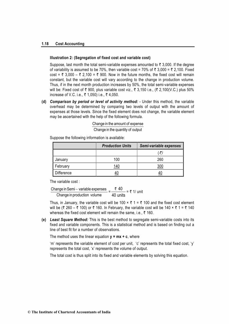
Illustration 2: (Segregation of fixed cost and variable cost)
Suppose, last month the total semi-variable expenses amounted to ` 3,000. If the degree
of variability is assumed to be 70%, then variable cost = 70% of ` 3,000 = ` 2,100. Fixed
cost = ` 3,000 – ` 2,100 = ` 900. Now in the future months, the fixed cost will remain
constant, but the variable cost will vary according to the change in production volume.
Thus, if in the next month production increases by 50%, the total semi-variable expenses
will be: Fixed cost of ` 900, plus variable cost viz., ` 3,150 i.e., (` 2,100(V.C.) plus 50%
increase of V.C. i.e., ` 1,050) i.e., ` 4,050.
(d) Comparison by period or level of activity method: - Under this method, the variable
overhead may be determined by comparing two levels of output with the amount of
expenses at those levels. Since the fixed element does not change, the variable element
may be ascertained with the help of the following formula.
output ofquantity the in Change
expense ofamount the in Change
Suppose the following information is available:
Production Units Semi-variable expenses
(`)
January 100 260
February 140 300
Difference 40 40
The variable cost :
volume production in Change
expenses variable Semi in Change −=
40
40 units
`= ` 1/ unit
Thus, in January, the variable cost will be 100 × ` 1 = ` 100 and the fixed cost element
will be (` 260 – ` 100) or ` 160. In February, the variable cost will be 140 × ` 1 = ` 140
whereas the fixed cost element will remain the same, i.e., ` 160.
(e) Least Square Method: This is the best method to segregate semi-variable costs into its
fixed and variable components. This is a statistical method and is based on finding out a
line of best fit for a number of observations.
The method uses the linear equation y = mx + c, where
‘m’ represents the variable element of cost per unit, ‘c’ represents the total fixed cost, ‘y’
represents the total cost, ‘x’ represents the volume of output.
The total cost is thus split into its fixed and variable elements by solving this equation.
© The Institute of Chartered Accountants of India
Basic Concepts 1.19
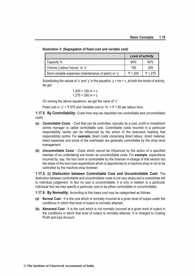
Illustration 3: (Segregation of fixed cost and variable cost)
Level of activity
Capacity % 60% 80%
Volume (Labour hours) or ‘x’ 150 200
Semi-variable expenses (maintenance of plant) or ‘y’ ` 1,200 ` 1,275
Substituting the values of ‘x’ and ‘y’ in the equation, y = mx + c, at both the levels of activity,
we get
1,200 = 150 m + c
1,275 = 200 m + c
On solving the above equations, we get the value of ‘c’
Fixed cost or ‘c’ = ` 975 and Variable cost or ‘m’ = ` 1.50 per labour hour.
1.17.5 By Controllability: Costs here may be classified into controllable and uncontrollable
costs.
(a) Controllable Costs: - Cost that can be controlled, typically by a cost, profit or investment
centre manager is called controllable cost. Controllable costs incurred in a particular
responsibility centre can be influenced by the action of the executive heading that
responsibility centre. For example, direct costs comprising direct labour, direct material,
direct expenses and some of the overheads are generally controllable by the shop level
management.
(b) Uncontrollable Costs - Costs which cannot be influenced by the action of a specified
member of an undertaking are known as uncontrollable costs. For example, expenditure
incurred by, say, the tool room is controllable by the foreman in-charge of that section but
the share of the tool-room expenditure which is apportioned to a machine shop is not to be
controlled by the machine shop foreman.
1.17.5. (i) Distinction between Controllable Cost and Uncontrollable Cost: The
distinction between controllable and uncontrollable costs is not very sharp and is sometimes left
to individual judgement. In fact no cost is uncontrollable; it is only in relation to a particular
individual that we may specify a particular cost to be either controllable or uncontrollable.
1.17.6 By Normality: According to this basis cost may be categorised as follows:
(a) Normal Cost - It is the cost which is normally incurred at a given level of output under the
conditions in which that level of output is normally attained.
(b) Abnormal Cost - It is the cost which is not normally incurred at a given level of output in
the conditions in which that level of output is normally attained. It is charged to Costing
Profit and loss Account.
© The Institute of Chartered Accountants of India

1.20 Cost Accounting
1.17.7 By Costs for Managerial Decision Making: According to this basis cost may be
categorised as follows:
(a) Pre-determined Cost - A cost which is computed in advance before production or operations start, on the basis of specification of all the factors affecting cost, is known as a pre-determined cost.
(b) Standard Cost - A pre-determined cost, which is calculated from managements ‘expected standard of efficient operation’ and the relevant necessary expenditure. It may be used as a basis for price fixing and for cost control through variance analysis.
(c) Marginal Cost - The amount at any given volume of output by which aggregate costs are changed if the volume of output is increased or decreased by one unit.
(d) Estimated Cost - Kohler defines estimated cost as “the expected cost of manufacture, or acquisition, often in terms of a unit of product computed on the basis of information available in advance of actual production or purchase”. Estimated costs are prospective costs since they refer to prediction of costs.
(e) Differential Cost - (Incremental and decremental costs). It represents the change (increase or decrease) in total cost (variable as well as fixed) due to change in activity level, technology, process or method of production, etc. For example if any change is proposed in the existing level or in the existing method of production, the increase or decrease in total cost or in specific elements of cost as a result of this decision will be known as incremental cost or decremental cost.
(f) Imputed Costs - These costs are notional costs which do not involve any cash outlay. Interest on capital, the payment for which is not actually made, is an example of imputed cost. These costs are similar to opportunity costs.
(g) Capitalised Costs - These are costs which are initially recorded as assets and subsequently treated as expenses.
(h) Product Costs - These are the costs which are associated with the purchase and sale of goods (in the case of merchandise inventory). In the production scenario, such costs are associated with the acquisition and conversion of materials and all other manufacturing inputs into finished product for sale. Hence, under marginal costing, variable manufacturing costs and under absorption costing, total manufacturing costs (variable and fixed) constitute inventoriable or product costs.
(i) Opportunity Cost - This cost refers to the value of sacrifice made or benefit of opportunity foregone in accepting an alternative course of action. For example, a firm financing its expansion plan by withdrawing money from its bank deposits. In such a case the loss of interest on the bank deposit is the opportunity cost for carrying out the expansion plan.
(j) Out-of-pocket Cost - It is that portion of total cost, which involves cash outflow. This cost concept is a short-run concept and is used in decisions relating to fixation of selling price in recession, make or buy, etc. Out–of–pocket costs can be avoided or saved if a particular proposal under consideration is not accepted.
© The Institute of Chartered Accountants of India

Basic Concepts 1.21
(k) Shut down Costs - Those costs, which continue to be, incurred even when a plant is temporarily shutdown e.g. rent, rates, depreciation, etc. These costs cannot be eliminated with the closure of the plant. In other words, all fixed costs, which cannot be avoided during the temporary closure of a plant, will be known as shut down costs.
(l) Sunk Costs - Historical costs incurred in the past are known as sunk costs. They play no role in decision making in the current period. For example, in the case of a decision relating to the replacement of a machine, the written down value of the existing machine is a sunk cost and therefore, not considered.
(m) Absolute Cost - These costs refer to the cost of any product, process or unit in its totality. When costs are presented in a statement form, various cost components may be shown in absolute amount or as a percentage of total cost or as per unit cost or all together. Here the costs depicted in absolute amount may be called absolute costs and are base costs on which further analysis and decisions are based.
(n) Discretionary Costs – Such costs are not tied to a clear cause and effect relationship between inputs and outputs. They usually arise from periodic decisions regarding the maximum outlay to be incurred. Examples include advertising, public relations, executive training etc.
(o) Period Costs - These are the costs, which are not assigned to the products but are charged as expenses against the revenue of the period in which they are incurred. All non-manufacturing costs such as general & administrative expenses, selling and distribution expenses are recognised as period costs.
(p) Engineered Costs - These are costs that result specifically from a clear cause and effect relationship between inputs and outputs. The relationship is usually personally observable. Examples of inputs are direct material costs, direct labour costs etc. Examples of output are cars, computers etc.
(q) Explicit Costs - These costs are also known as out of pocket costs and refer to costs involving immediate payment of cash. Salaries, wages, postage and telegram, printing and stationery, interest on loan etc. are some examples of explicit costs involving immediate cash payment.
(r) Implicit Costs - These costs do not involve any immediate cash payment. They are not recorded in the books of account. They are also known as economic costs.
1.18 Methods of Costing
Different industries follow different methods of costing because of the differences in the nature
of their work. The various methods of costing are as follows:
Methods Description
Job Costing In this method of costing, cost of each job is ascertained separately. It is suitable in all cases where work is undertaken
© The Institute of Chartered Accountants of India

1.22 Cost Accounting
on receiving a customer’s order like a printing press, motor workshop, etc.
Batch Costing It is the extension of job costing. A batch may represent a number of small orders passed through the factory in batch. Each batch here is treated as a unit of cost and thus separately costed. Here cost per unit is determined by dividing the cost of the batch by the number of units produced in the batch.
Contract Costing Here the cost of each contract is ascertained separately. It is suitable for firms engaged in the construction of bridges, roads, buildings etc.
Single or Output Costing Here the cost of a product is ascertained, the product being the only one produce like bricks, coals, etc.
Process Costing Here the cost of completing each stage of work is ascertained, like cost of making pulp and cost of making paper from pulp. In mechanical operations, the cost of each operation may be ascertained separately; the name given is operation costing.
Operating Costing It is used in the case of concerns rendering services like transport, supply of water, retail trade etc.
Multiple Costing It is a combination of two or more methods of costing outlined above. Suppose a firm manufactures bicycles including its components; the parts will be costed by the system of job or batch costing but the cost of assembling the bicycle will be computed by the Single or output costing method. The whole system of costing is known as multiple costing.
The following table summarises the various methods of costing applied in different industries:
Nature of Output Method Cost Examples of Industries
A Series of Processes
Process costing or Operation Costing
For each process Sugar
Construction of building
Contract Costing For each contract Real estate
Similar units of a Single Product, produced by Single Process
Unit or output or Single Costing
For the entire activity, but averaged for the output
Cold Drinks
© The Institute of Chartered Accountants of India

Basic Concepts 1.23
Rendering of Services
Operating Costing For all services Hospitals
Customer Specifications: single Unit
Job Costing For each order/ assignment/job
Advertising
Consisting of multiple varieties of activities and processes
Multiple Costing Combination of any method
Car Assembly
1.19 Techniques of Costing
For ascertaining cost, following types of costing are usually used.
Techniques Description
Uniform Costing When a number of firms in an industry agree among themselves to follow the same system of costing in detail, adopting common terminology for various items and processes they are said to follow a system of uniform costing.
Advantages of such a system are that
i. A comparison of the performance of each of the firms can be made with that of another, or with the average performance in the industry.
ii. Under such a system it is also possible to determine the cost of production of goods which is true for the industry as a whole. It is found useful when tax-relief or protection is sought from the Government.
Marginal Costing It is defined as the ascertainment of marginal cost by differentiating between fixed and variable costs. It is used to ascertain effect of changes in volume or type of output on profit.
Standard Costing and Variance Analysis
It is the name given to the technique whereby standard costs are pre-determined and subsequently compared with the recorded actual costs. It is thus a technique of cost ascertainment and cost control. This technique may be used in conjunction with any method of costing. However, it is especially suitable where the manufacturing method involves production of standardised goods of repetitive nature.
Historical Costing It is the ascertainment of costs after they have been incurred. This type of costing has limited utility.
Post Costing: It means ascertainment of cost after production is completed.
© The Institute of Chartered Accountants of India

1.24 Cost Accounting
Continuous costing: Cost is ascertained as soon as the job is completed or even when the job is in progress.
Direct Costing It is the practice of charging all direct costs to operations, processes or products leaving all indirect costs to be written off against profits in which they arise.
Absorption Costing It is the practice of charging all costs, both variable and fixed to operations, processes or products. This differs from marginal costing where fixed costs are excluded.
1.20 Coding System
1.20.1 Codes: The Chartered Institute of Management Accountants has defined a code as “a
system of symbols designed to be applied to a classified set of items to give a brief account
reference, facilitating entry collation and analysis”
Hence cost classification forms the basis of any cost coding. It helps us understand the
characteristic of any cost through a short symbolised form.
1.20.2 Composite Codes (Example): A company has devised a system of codification in
which the first three digits indicate the nature of the expenditure and the last three digits the
cost centre or cost unit to be charged e.g. if the first digit is 1, the system implies that it refers
to raw material and if the number is 2 it represents a labour cost. The second and third numbers
relating to 1 i.e., raw material, provide details of the type e.g., whether the raw material is an
electronic component (number 4), mechanical component (number 1) consumables(number 2)
or packing (number 3) and the name respectively. Hence the description of a cost with a code
146.729 shall be understood as follows:
Since the first number is 1 the cost refers to raw material cost
The second number being 4 indicates that the raw material is an electronic component.
The third number 6 refers to the description which according to the company’s codification
refers to Diodes.
The last three numbers provide details of the cost centre e.g. the first number provides details of the
location of the plant, the second number gives detail of the department (machining or assembly or
something else) and the third number indicates whether the cost is direct or indirect.
1.20.3 Advantages of a coding system: The following are some of the advantages of a
well-designed coding system:
(a) Short and simple: Since the code is, most of the times, briefer than a description, it saves time when systems are worked upon manually and in case the system is computerised it reduces the data storage capacity. The illustration above demonstrates this advantage very clearly.
© The Institute of Chartered Accountants of India

Basic Concepts 1.25
(b) Clarity: A code helps in reducing ambiguity. In case two professionals understand the same item differently a code will help them objectively.
(c) Computer friendly: Unlike detailed descriptions, a code facilitates data processing in computerised systems.
1.20.4 The requirements for an efficient coding system
(a) Unique: Every number used in the code should be unique and certain, i.e. it should be
easily identified from the structure of the code.
(b) Flexibility: Elasticity and comprehensiveness is an absolute must for a well designed
coding system. It should be possible to identify a code for every item and the coding system
should be capable of expanding to accommodate new items.
(c) Brief: The code should be brief and meaningful.
(d) Centralised: The maintenance of the coding system should be centrally controlled. It
should not be possible for individuals to independently add new codes to the existing
coding system.
(e) Similarity: Codification systems should be of the same length. This makes errors easier
to spot and it assists computerised data processing.
1.21 Summary
Classification of Costs
Nature of classification
Classified Costs
Examples
Nature of Element
Material: Cost of Material used in production Cost of Raw Material
Labour: Cost of Workers Wages and Salary
Expenses: Costs other than Material and Labour
Power, Office Maintenance
Traceability to Object
Direct Costs: Which can be allocated directly to the product
Wood in case of Furniture
Indirect Costs: Which cannot be directly allocated to the product
Nails used in Furniture
Functions Production Costs Cost of whole process of Production
Direct Materials and Conversion Cost.
Selling Costs: Cost for creating demand of the product produced
Advertising Expenses
Distribution Costs: Costs starting from packing of the product till reconditioning of empty products
Freight and Transportation Costs on Sales
© The Institute of Chartered Accountants of India

1.26 Cost Accounting
Administrative Costs: Cost of formulating policy, controlling the organisation, costs not directly related to production
Salary of Office Staff
Development Costs: Development Costs for trial Run
Research Costs
Pre- Production Costs: Costs starting with implementation of decisions and ending with the commencement of the production process
Direct Labour and Factory Overheads
Conversion Costs: Cost of transforming direct material into Finished Products
Direct Labour and Overheads
Product Costs: Costs necessary for production
Cost of purchase
Variability Fixed Costs: Cost which remains constant in total
Factory Rent
Variable Costs: Costs which changes with production
Cost of Raw Material
Semi- Variable Costs: Costs which are partly fixed and partly variable
Repair and Maintenance
Controllability Controllable Costs: Costs which can be influenced by the action of a specific member of an undertaking
Raw Material, Labour Costs, controlled by shop level management
Uncontrollable Costs: Costs which cannot be influenced by the action of a specific member.
Fixed Costs- Rent
Normality Normal Costs: Costs which are expected to be incurred in normal routine
Raw Material Costs
Abnormal Costs: Costs which are over and above normal costs
Cost of Wastes
Decision Making
Relevant Costs (Marginal Costs, Differential Costs, Opportunity Costs, Out of Pocket): Costs which are relevant and useful for decision making
Cost of Best Possible Use
Irrelevant Costs (Sunk costs, Committed costs, Fixed costs): Costs which are not relevant or useful to decision making
Costs incurred in the past - Advance Payment
Cash Outflow Explicit Costs: Costs involving immediate payment of cash
Purchase of Raw material.
Implicit Costs: Costs not involving immediate cash payment
Depreciation
© The Institute of Chartered Accountants of India

Basic Concepts 1.27
Types of Costing
Type Description
Uniform Costing Standardised principles and practices of costing are used by a number of different industries.
Marginal Costing Only Variable Costs or costs directly linked are charged to the product or process
Standard Costing Standard Costs are compared with actual costs, to determine variances
Historical Costing Where costs are recorded after they have incurred
Direct Costing Direct Costs are charged to the product or process, Indirect Costs are charged to the profit from the product or process.
Absorption Costing All costs (variable and Fixed) are charged to the product or process
Methods of Costing
Method Description
Job costing Where all costs can be directly charged to a specific job
Batch Costing Where all costs can be directly charged to a group of products (batch)
Contract Costing Similar to Job costing, but in this case the job is larger than job costing.
Single or Output Costing
Cost ascertainment for a single product.
Process Costing The cost of production at each stage is ascertained separately
Operating Costing Ascertainment of Costs in cases where services are rendered
Multiple Costing Combination of two or more methods of costing, used where the nature of the product is complex and method cannot be ascertained
© The Institute of Chartered Accountants of India

2 Material
Learning Objectives
After studying this chapter you will be able to:
Understand the concept of materials,
Understand its need and importance.
Describe the procedures involved in procuring, storing and issuing material.
Differentiate amongst the various methods of valuing material.
Evaluate different methods of pricing material issues, material received and material return.
Understand the meaning and accounting treatment for normal and abnormal loss of 0material.
Understand the meaning and the accounting treatment of waste, scrap, spoilage and
defectives.
2.1 Introduction
We have acquired a basic knowledge about the concepts, objectives, advantages, methods
and elements of cost. We shall now study each element of cost separately begin with material.
The general meaning of material is all commodities/ physical objects supplied to an
organization. It may be direct material or indirect material. Materials constitute a very
significant portion of total cost of finished product. A proper recording and control over the
material costs is very essential. Importance of proper recording and control of material are
following:
(a) Dependence of the Quality of finished product: The exact quality of raw materials re-
quired should be determined according to the required quality of the finished product.
Quality and cost both should be given equal consideration.
(b) Price of the product: The price paid should be the minimum possible otherwise the
higher cost of the finished products would make the product uncompetitive in the market.
(c) Continuity in production: There should not be any interruption in the production
process for want of materials and stores, including small inexpensive items like
lubricating oil for a machine.
© The Institute of Chartered Accountants of India

Material 2.2
(d) Cost of holding material: There should not be over stocking of materials because this
would result in loss of interest charges, higher warehouse charges, deterioration in
quality and losses due to obsolescence
(e) Wastages: Wastage and losses while the materials are in store and during the process
of manufacture should be avoided as far as possible; and
(f) Regular information about resources: It may also be added that information about
availability of materials and stores should be continuously available so that production
may be planned properly and the required materials purchased in time.
2.2 Material Control
The publication of the Chartered Institute of Management Accountants (CIMA) on Inventory
Control defines it as “The function of ensuring that sufficient goods are retained in stock to
meet all requirements without carrying unnecessarily large stocks.”
2.2.1 Objectives of system of material control: The objectives of a system of material control are the following:
(i) Minimising interruption in production process: Ensuring that no activity, particularly
production, suffers from interruption for want of materials and stores. It should be noted
that this requires constant availability of every item that may be needed howsoever small
its cost may be.
(ii) Cost of Material: Seeing to it that all the materials and stores are acquired at the lowest
possible price considering the quality that is required and considering other relevant
factors like reliability in respect of delivery, etc. Holding cost should also be tried to be
minimized.
(iii) Reduction in Wastages: Avoidance of unnecessary losses and wastages that may arise
from deterioration in quality due to defective or long storage or from obsolescence. It may
be noted that losses and wastages in the process of manufacture, concern the
production department.
(iv) Adequate Information: Maintenance of proper records to ensure that reliable
information is available for all items of materials and stores that not only helps in
detecting losses and pilferages but also facilitates proper production planning.
(v) Completion of order in time: Proper material management is very necessary for
fulfilling orders of the firm. This adds to the goodwill of the firm.
2.2.2 Requirements of material control: Material control requirements can be summarised as follows:—
1. Proper co-ordination of all departments involved viz., finance, purchasing, receiving,
inspection, storage, accounting and payment.
© The Institute of Chartered Accountants of India

2.3 Cost Accounting
2. Determining purchase procedure to see that purchases are made, after making suitable
enquiries, at the most favourable terms to the firm.
3. Use of standard forms for placing the order, noting receipt of goods, authorising issue of
the materials etc.
4. Preparation of budgets concerning materials, supplies and equipment to ensure economy
in purchasing and use of materials.
5. Operation of a system of internal check so that all transactions involving materials,
supplies and equipment purchases are properly approved and automatically checked.
6. Storage of all materials and supplies in a well designated location with proper
safeguards.
7. Operation of a system of perpetual inventory together with continuous stock checking so that
it is possible to determine at any time the amount and value of each kind of material in stock.
8. Operation of a system of stores control and issue so that there will be delivery of materials
upon requisition to departments in the right amount at the time they are needed.
9. Development of system of controlling accounts and subsidiary records which exhibit
summary and detailed material costs at the stage of material receipt and consumption.
10. Regular reports of materials purchased, issue from stock, inventory balances, obsolete
stock, goods returned to vendors, and spoiled or defective units.
2.2.3 Elements of Material Control: Material control is a systematic control over the procurement, storage and usage of material so as to maintain an even flow of material.
Material control involves efficient functioning of the following operations:
Purchasing of materials
Receiving of materials
Inspection of materials
Storage of materials
Issuing materials
Maintenance of inventory records
Stock audit.
2.3 Materials Procurement Procedure
Material procurement procedure can be understood with help of the following diagram. Documents required and the departments who initiate these documents are shown sequentially.
© The Institute of Chartered Accountants of India

Material 2.4
Engineering/ Planning Department
1. Bill o
f Materials
2. Material Requisition Note
3. Purchase Requisition
Production Department / Work Shop
Store Purchase Department
4. Ten
der o
r Req
uest fo
r pro
po
sal (RF
P)
5. Q
uo
tati
on
6. Pu
rchase O
rder
r
7. Performa Invoice
8. Payment and Form-C etc.
9. Invoice
10. Goods delivery with Challan or/and Invoice
11. Go
od
s Received
No
te
12. Material R
eturn
ed N
ote
12. Material Returned Note
13. Material A
bstract
Diagram: Material Procurement Procedure
Supplier(s) Cost/ Accounting Department
© The Institute of Chartered Accountants of India

2.5 Cost Accounting
2.3.1 Bill of Materials: It is also known as Materials Specification List or simply Materials
List. It is a schedule of standard quantities of materials required for any job or other unit of
production. A comprehensive Materials List should rigidly lay down the exact description and
specifications of all materials required for a job or other unit of production and also required
quantities so that if there is any deviation from the standard list, it can easily be detected. The
materials specification list is prepared by the Engineering or Planning Department in a
standard form. The numbers of copies prepared vary according to the requirement of each
business. Generally Bill of Material is sent to Production control department, Store
department, Cost/ Accounting department and a copy retained with engineering or planning
department. A proforma of Bill of Materials is as follows:
Bill of Materials
Job No. ............................................. No. ......................................
Department authorised ............... Date ...................................
Sl. Code Description Qty. Date of Rate Amount
No. No. issue & Qty. ` `
issued
Date Qty.
Authorised by .................................................. Received by .........................
Checked by ..........................
Store Keeper’s signature ............................. Cost clerk .............................
The advantages of using “bill of materials”, by the concerned departments may be
summed up as follows:—
Stores Department:
1. A bill of material serves as an important basis of preparing material purchase requisitions
by stores department.
2. It acts as an authorisation for issuing total material requirement.
3. The clerical activity is reduced as the stores clerk issues the entire/part of the material
requirement to the users if the details of material asked are present in the bill of
materials.
© The Institute of Chartered Accountants of India

Material 2.6
Cost Accounts Department:
1. Bill of material, is used by Cost Accounts department for preparing an estimate/budget of
material cost for the job/process/operation, it is meant.
2. It may be used as a device for controlling the excess cost of material used. This is done
after determining material variances and ascertaining the reasons for their occurrence.
Production Control Department:
1. Bill of material may be used by this department for controlling usage of materials.
2. Its usage saves time which otherwise would have been wasted for preparing separate
requisitions of material.
Engineering or Planning department: As stated earlier this department prepares the
materials list in a standard form. A copy of list is sent to stores, cost accounts and production
control department.
2.3.2 Material Requisition Note: It is also known as material requisition slip, It is the
voucher of the authority regarding issue of materials for use in the factory or in any of its
departments. Generally it is prepared by the production department and materials are
withdrawn on the basis of material requisition list or bill of materials. If no material list has
been prepared, it is desirable that the task of the preparation of material requisition notes be
left to the planning department or by the department requires the materials. Usually, a
foreman’s authority is enough but, in the case of costly materials, it would be desirable to have
such requisitions duly approved by some higher authority, like the superintendent or works
manager before these are presented to Stores. Apart from sending a material requisition to
store a copy is sent to cost accounting department and one copy is retained as office copy.
A specimen form of the Material Requisition is shown below:
Material Requisition Note
Work Order No. ............................ No. ..........................................
Department ..................................... Date .......................................
Item No. Particulars Qnty. Rate Amount ` `
Store-keeper Workman receiving Foreman S.L. Clerk the material
© The Institute of Chartered Accountants of India

2.7 Cost Accounting
Difference between Bill of Materials and Material Requisition Note:
Bill of Materials Material Requisition Note
1. It is the document prepared by the drawing office.
1. It is prepared by the Foreman of the consuming department.
2. It is a complete schedule of component parts and raw materials required for a particular job or work order.
2. It is a document authorizing Store-keeper to issue materials to the consuming department.
3. It often serves the purpose of a Stores Requisition as it shows the complete schedule of materials required for a particular job i.e. it can replace stores requisition.
3. It cannot replace a bill of materials.
4. It can be used for the purpose of quotations.
4. It is useful in arriving historical cost only.
5. It helps in keeping a quantitative control on materials drawn through stores Requisition.
5. It shows the material actually drawn from stores.
2.3.3 Purchase Requisition: Since the materials purchased will be used by the production
departments, there should be constant co-ordination between the purchase and production
departments. A purchase requisition is a form used for making a formal request to the
purchasing department to purchase materials. This form is usually filled up by the store keeper
for regular materials and by the departmental head for special materials (not stocked as
regular items). The requisition form is duly signed by either works manager or plant
superintendent, in addition to the one originating it. At the beginning a complete list of
materials and stores required should be drawn up, the list should have weekly consumption
figures. It should be gone through periodically so that necessary deletion and addition may be
made. If there is any change in the rate of consumption per week (say, due to extra shift being
worked), the purchase department should be informed about the new figures. Once an item
has been included in the standard list, it becomes the duty of the purchase department to
arrange for fresh supplies before existing stocks are exhausted. But if the production
department requires some new material, it should make out an indent well in time and send it
to the purchase department for necessary action.
For control over buying of regular store materials it is necessary to determine their maximum, minimum, reorder level and economic order quantities. The use of economic order quantities and various levels constitutes an adequate safeguard against improper indenting of regular materials. In respect of special materials, required for a special order or purpose, it is desirable that the technical department concerned should prepare materials specifications list specifying the quantity, size and order specifications of materials to be drawn from the store and those to be specially procured. It may originate either in the stores department in connection with regular stock of materials or in the production planning or in other technical
© The Institute of Chartered Accountants of India

Material 2.8
departments concerned in respect of special materials. Its purpose is to request and authorise the purchase department to order to procure the materials specified in stated quantities. It should be made out in triplicate and send to following.
Purchase Requisition (Regular/Special)
(Use a separate form for each item)
No.................. Department.................................
Date.............
Purchase................... Date by which material required...............................
Description of Quantity Exact specification
Materials required required
………………
Indentor
For use in purchase department
Firm 1. 2. 3. Order
Quotations No. & Date...........................
.......................................................................................
Price (including charges) With......................................
.......................................................................................
Price...............................
Date of Delivery Date of dly...................
.......................................................................................
Remarks Purchase Manager
2.3.4 Inviting Tender/ Requesting for proposal (RFP): After receipt of purchase
requisition from the store department or other competent departments, role of purchasing
department comes into play. If a concern can afford or the size of the concern is big enough,
there should be a separate purchase department for all purchases to be made on behalf of all
other departments. Such a department is bound to become expert in the various matters to be
© The Institute of Chartered Accountants of India
2.9 Cost Accounting
attended to, for examples— units of materials to be purchased and licences to be obtained,
transport, sources of supply, probable price etc.
Materials purchase department in a business house is confronted with the following issues:
(i) What to purchase?
(ii) When to purchase?
(iii) How much to purchase?
(iv) From where to purchase.
(v) At what price to purchase.
To overcome these questions, purchase department make an enquiry into the market for the
required material. The process of gathering information about the rate, quantity, technology,
services and support etc., purchase department sent RFP to selected vendors in case if
purchase policy allows this practice. Some organizations follow the open and transparent
purchase policy and invite quotationsS from the interested vendors. This process is called
Tender Notification or Invitation of Tender.
2.3.5 Selection of Quotation/ Proposal: After invitation of tender from the vendors, interested
vendors who are fulfilling all the criteria mentioned in the tender notice send their price quotations/
proposals to the purchase department. On the receipt of quotations a comparative statement is
prepared. For selecting material suppliers the factors which the purchase department keeps in
its mind are—price; quantity; quality offered; time of delivery; mode of transportation; terms of
payment; reputation of supplier; etc. In addition to the above listed factors purchase manager
obtains other necessary information from the statement of quotations; past records, buyer
guides etc. for finally selecting material suppliers.
2.3.6 Preparation and execution of Purchase Orders: Having decided on the best
quotation that should be accepted, the purchase manager or concerned officer proceeds to
issue the formal purchase order. It is a written request to the supplier to supply certain
specified materials at specified rates and within a specified period. Generally copies of
purchase order are given to Store or order indenting department, receiving department and
cost accounting department. A copy of the purchase order, alongwith relevant purchase requi-
sitions, is held in the file of the department to facilitate the follow-up, of the delivery and also
for approving the invoice for payment.
2.3.7 Receipt and inspection of materials: After execution of purchase order and
advance payment (if terms of quotation so specified), necessary arrangement is made to
receive the delivery of materials (in case of inter-state purchase way bill (e.g. Form-C) is get
issued by the purchase or accounting department). After receipt of materials along with
challan or/ and invoice, Receiving department arrange to inspect the materials for its
conformity with purchase order. After satisfactory inspection materials are received and Goods
Received Note is issued. If some materials are not found in good condition or not in conformity
with the purchase order are returned back to the vendor alongwith a Material Returned Note.
© The Institute of Chartered Accountants of India

Material 2.10
2.3.7.1 Goods Received Note: If everything is in order and the supply is considered
suitable for acceptance, the Receiving department prepares a Receiving Report or Material
Inward Note or Goods Received Note. Generally it is prepared in quadruplicate, the copies
being distributed to purchase department, store or order indenting department, receiving
depart and accounting department.
A specimen form of the receiving report is given below:
Goods Received Note
Received from.............................. No. ..............
Order No. .................. Date............................
Amount
Quantity Code Description Amount Charges Total Remarks
due to ` `
supplier
`
Inspector....................... Store Keeper..................................
Receiver........................ Store Ledger Clerk......................
2.3.7.2 Material Returned Note : Sometimes materials have to be returned to suppliers
after these have been received in the factory. Such returns may occur before or after the
preparation of the receiving report. If the return takes place before the preparation of the
receiving report, such material obviously would not be included in the report and hence not
debited in the stores books and ledgers. In that case, no adjustment in the account books
would be necessary. But if the material is returned after its entry in the receiving report, a
suitable document must be drawn up in support of the credit entry so as to exclude from the
Stores of Material Account the value of the materials returned back. This document usually
takes the form of a Material Returned Note or Material outward return note.
The Material outward return note is drawn up by the Stores or the Despatch Department. Five
copies of it are usually prepared; two for the supplier (one of which is to be sent back by the
supplier after he has signed the same), one for Store, one for Cost (stores) Ledger and one
copy to be retained in the Material outward return book.
2.3.8 Checking and passing of bills for payment: The invoice received from the supplier
is sent to the stores accounting section to check authenticity and mathematical accuracy. The
quantity and price are also checked with reference to goods received note and the purchase
order respectively. The stores accounting section after checking its accuracy finally certifies
and passes the invoice for payment. In this way the payment is made to supplier.
© The Institute of Chartered Accountants of India

2.11 Cost Accounting
2.4 Valuation of Material Receipts
After the procurement of materials from the supplier actual material cost is calculated. Ascertainment of cost of material purchased is called valuation of materials. Cost of material includes cost of purchase net of trade discounts, rebates, duty draw-back, Cenvat credit availed, etc. and other costs incurred in bringing the inventories to their present location and condition. The invoice of material purchased from the market sometime contain items such as trade discount, quantity discount, freight, duty, insurance, cost of containers, sales tax, excise duty, cash discount etc.
Treatment of items associated with purchase of materials is tabulated as below
Sl no.
Items Treatment
Discounts and Subsidy
(i) Trade Discount Trade discount is deducted from the purchase price if it is not shown as deduction in the invoice.
(ii) Quantity Discount Like trade discount quantity discount is also shown as deduction from the invoice. It is deducted from the purchase price if not shown as deduction.
(iii) Cash Discount Cash discount is not deducted from the purchase price. It is treated as interest and finance charges.
(iv) Subsidy/ Grant/ Incentives
Any subsidy/ grant/ incentive received from the Government or from other sources deducted from the cost of purchase.
Duties and Taxes
(v) Road Tax/ Toll Tax Road tax/ Toll tax if paid by the buyer then it is included with the cost of purchase.
(vi) Octroi/ Entry Tax Octroi/ Entry tax is collected by the Panchayats/ local authorities. It is added with cost of purchase if it is borne by the buyer.
(vii) Central Sales Tax (CST)
Central Sales Tax (CST) is paid on inter-state sale and collected from the buyers. The buyer is not getting any credit for tax paid hence it is added with cost of purchase.
(viii) State Sales tax or Value Added Tax (VAT)
State Sales Tax/ VAT is paid on intra-state sale and collected from the buyers. It is excluded from the cost of purchase if credit for the same is available. Unless mentioned specifically it should not form part of cost of purchase.
© The Institute of Chartered Accountants of India

Material 2.12
(ix) Excise Duty Excise duty is paid on manufacture of goods and collected from the buyer. It is excluded from the cost of purchase if credit (CENVAT) is available for the same. Unless mentioned specifically excise duty is not added with the cost of purchase.
(x) Custom Duty Custom duty is paid on import of goods from outside India. It is added with the purchase cost.
(xi) Purchase Tax It is a tax paid on purchase of goods from unregistered supplier. Credit on purchase tax is available hence unless specifically mentioned it is not added with the cost of purchase.
Penalty and Charges
(xii) Demurrage Demurrage is a penalty imposed by the transporter for delay in uploading or offloading of materials. It is an abnormal cost and not included with cost of purchase
(xiii) Detention charges/ Fine
Detention charges/ fines are imposed for non compliance of rule or law by any statutory authority. It is an abnormal cost and not included with cost of purchase
(xiv) Penalty Penalty of any type is not included with the cost of purchase
Other expenditures
(xv) Insurance charges Insurance charges are paid for protecting goods during transit. It is added with the cost of purchase.
(xvi) Commission or brokerage paid.
Commission or brokerage paid is added with the cost of purchase.
(xvii) Freight inwards It is added with the cost of purchase as it is directly attributable to procurement of material.
(xviii) Cost of containers Treatment of cost of containers are as follows:
Non-returnable containers: The cost of containers is added with the cost of purchase of materials.
Returnable Containers: If on return of containers cost of containers is returned back then in this case cost of containers is not added with the cost of purchase.
If the amount of refund on returning the container is less than the amount paid then only short fall is added with the cost of purchase.
(xix) Shortage Shortage in materials are treated as follows:
Shortage due to normal reasons: Good units absorb
© The Institute of Chartered Accountants of India

2.13 Cost Accounting
the cost of shortage due to normal reasons. Losses due to breaking of bulk, evaporation, due to unavoidable conditions etc. are the reasons of normal loss.
Shortage due to abnormal reasons: shortage arises due to abnormal reasons such as material mishandling, pilferage, due to avoidable reasons are not absorbed by the good units. Losses due to abnormal reasons are debited to costing profit and loss account.
Illustration 1: (Valuation of material)
An invoice in respect of a consignment of chemicals A and B provides the following information:
(`)
Chemical A: 10,000 kgs. at ` 10 per kg. 1,00,000
Chemical B: 8,000 kgs. at ` 13 per kg. 1,04,000
Central Sales tax @ 2% 4,080
Railway freight 3,840
Total cost 2,11,920
A shortage of 500 kgs. in chemical A and 320 kgs. in chemical B is noticed due to normal breakages. You are required to determine the rate per kg. of each chemical, assuming a provision of 2% for further deterioration.
Solution
Working:
Computation of effective quantity of each chemical available for use
Chemical A (kg.) Chemical B (kg.)
Quantity purchased 10,000 8,000
Less : Shortage due to normal breakages 500 320
9,500 7,680
Less : Provision for deterioration 2% 190 153.6
Quantity available 9,310 7,526.4
Statement showing the computation of rate per kg. of each chemical
Chemical A (`) Chemical B (`)
Purchase price 1,00,000 1,04,000
Add : Central Sales tax @2% 2,000 2,080
Add: Railway freight
© The Institute of Chartered Accountants of India

Material 2.14
(in the ratio of quantity purchased i.e., 5:4) 2,133 1,707
Total cost (A) 1,04,133 1,07,787
Effective Quantity (see working) (B) 9,310 kg. 7,526.4 kg.
Rate per kg. (A ÷ B) 11.19 14.32
Illustration 2: (Valuation of material)
At what price per unit would Part No. A 32 be entered in the Stores Ledger, if the following
invoice was received from a supplier:
Invoice (`)
200 units Part No. A 32 @ ` 5 1,000.00
Less : 20% discount (200.00)
800.00
Add : Excise duty @ 15% 120.00
920.00
Add : Packing charges (5 non-returnable boxes) 50.00
970.00
(i) A 2 per cent cash discount will be given if payment is made in 30 days.
(ii) Documents substantiating payment of excise duty is enclosed for claiming CENVAT credit.
Solution
Computation of cost per unit
(`)
Net purchase Price 800.00
Add : Packing charges (5 non-returnable boxes) 50.00
850.00
No. of units purchased 200 units
Cost per unit 4.25
Note: (i) Cash discount is treated as interest and finance charges hence, it is not considered
for valuation of material.
(ii) Excise duty is refundable; hence it will not be added to purchase cost.
2.5 Material Storage & Records
Proper storing of materials is of primary importance. It is not enough only to purchase material
of the required quality. If the purchased material subsequently deteriorates in quality because
of bad storage, the loss is even more than what might arise from purchase of bad quality
© The Institute of Chartered Accountants of India

2.15 Cost Accounting
materials. Apart from preservation of quality, the store-keeper also must ensure safe custody
of the material. It should be the function of store-keeper that the right quantity of materials
always should be available in stock.
2.5.1 Duties of store keeper: These can be briefly set out as follows:
(i) General control over store: Store keeper should keep control over all activities in
Stores department. He should check the quantities as mentioned in Goods received note
and with the purchased materials forwarded by the receiving department and to arrange
for the storage in appropriate places.
(ii) Safe custody of materials: Store keeper should ensure that all the materials are stored
in a safe condition and environment required to preserve the quality of the materials.
(iii) Maintaining records: Store keeper should maintain proper record of quantity received,
issued, balance in hand and transferred to/ from other stores.
(iv) Initiate purchase requisition: Store keeper should initiate purchase requisitions for the
replacement of stock of all regular stores items whenever the stock level of any item of
store approaches the re-order level fixed.
(v) Maintaining adequate level of stock: Store keeper should maintain adequate level of
stock at all time. He/ she should take all necessary action so that production could not be
interrupted due to lack of stock. Further he/ she should take immediate action for
stoppage of further purchasing when the stock level approaches the maximum limit. To
reserve a particular material for a specific job when so required.
(vi) Issue of materials: Store keeper should issue materials only against the material
requisition slip approved by the appropriate authority. He/ she should also refer to bill of
materials while issuing materials to requisitioning department.
(vii) Stock verification and reconciliation: Store keeper should verify the book balances
with the actual physical stock at frequent intervals by way of internal control and check
the any irregular or abnormal issues, pilferage, etc.
2.5.2 Store Records: The record of stores may be maintained in three forms:
Bin Cards
Stock Control Cards
Store Ledger
Bin Cards: Bin refers to a box/ container/ space where materials are kept. Card is placed with
each of the bin (space) to record the details of material like receipt, issue and return. The first two
forms are records of quantities received, issued and those in balance, but in the third record i.e.
store ledger, value of receipts, issues and closing balance is also maintained. Usually, records of
quantities i.e. Bin cards and Store Control Cards are kept by the store keeper in store department
while record of both quantity and value is maintained by cost accounting department.
Stock Control Cards: It is a record keeping document maintained by stores department for
© The Institute of Chartered Accountants of India
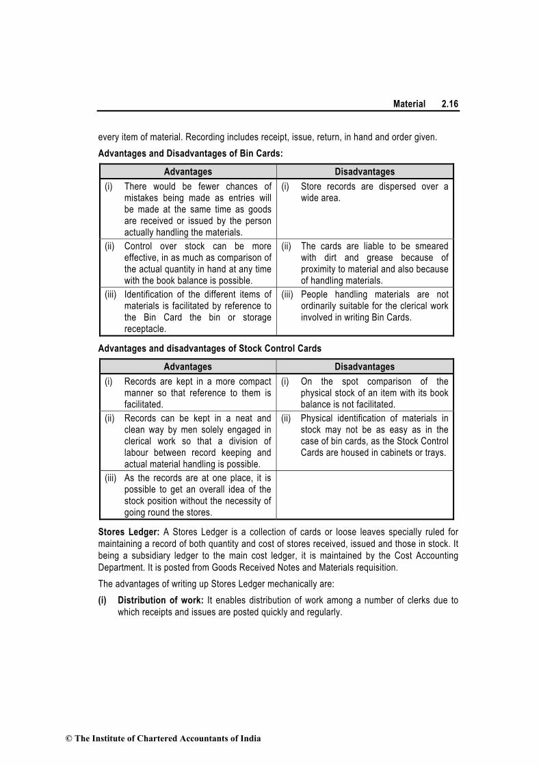
Material 2.16
every item of material. Recording includes receipt, issue, return, in hand and order given.
Advantages and Disadvantages of Bin Cards:
Advantages Disadvantages
(i) There would be fewer chances of mistakes being made as entries will be made at the same time as goods are received or issued by the person actually handling the materials.
(i) Store records are dispersed over a wide area.
(ii) Control over stock can be more effective, in as much as comparison of the actual quantity in hand at any time with the book balance is possible.
(ii) The cards are liable to be smeared with dirt and grease because of proximity to material and also because of handling materials.
(iii) Identification of the different items of materials is facilitated by reference to the Bin Card the bin or storage receptacle.
(iii) People handling materials are not ordinarily suitable for the clerical work involved in writing Bin Cards.
Advantages and disadvantages of Stock Control Cards
Advantages Disadvantages
(i) Records are kept in a more compact manner so that reference to them is facilitated.
(i) On the spot comparison of the physical stock of an item with its book balance is not facilitated.
(ii) Records can be kept in a neat and clean way by men solely engaged in clerical work so that a division of labour between record keeping and actual material handling is possible.
(ii) Physical identification of materials in stock may not be as easy as in the case of bin cards, as the Stock Control Cards are housed in cabinets or trays.
(iii) As the records are at one place, it is possible to get an overall idea of the stock position without the necessity of going round the stores.
Stores Ledger: A Stores Ledger is a collection of cards or loose leaves specially ruled for
maintaining a record of both quantity and cost of stores received, issued and those in stock. It
being a subsidiary ledger to the main cost ledger, it is maintained by the Cost Accounting
Department. It is posted from Goods Received Notes and Materials requisition.
The advantages of writing up Stores Ledger mechanically are:
(i) Distribution of work: It enables distribution of work among a number of clerks due to
which receipts and issues are posted quickly and regularly.
© The Institute of Chartered Accountants of India

2.17 Cost Accounting
(ii) Centralised record: It enables stock records to be centralised in case of an organisation
having a number of depots.
(iii) Testing of accuracy: The accuracy of posting can be mechanically tested more
conveniently.
(iv) Cost effective: The records are clearer and neater. Also the recurring cost of
maintaining them is much less than those kept manually.
(v) Control over stock: If up-to-date records are available, the management will be able to
exercise greater control over quantities held in stock from time to time which may result
in a great deal of saving in both the amount of investment in stock and their cost.
Difference between Bin Card & Stores Ledger
Bin Card Stores Ledger
It is maintained by the storekeeper in the store.
It is maintained in costing department.
It contains only quantitative details of material received, issued and returned to stores.
It contains information both in quantity and value.
Entries are made when transactions take place.
It is always posted after the transaction.
Each transaction is individually posted. Transactions may be summarized and then posted.
Inter-department transfers do not appear in Bin Card.
Material transfers from one job to another job are recorded for costing purposes.
2.6 Inventory Control
The main objective of inventory control is to achieve maximum efficiency in production and
sales with the minimum investment in inventory. Inventory comprises of stocks of raw
materials, stores & consumables, work-in-progress, and finished products. The techniques
commonly applied for inventory control are as follows:
Techniques of Inventory control:
(i) Setting of various stock levels.
(ii) ABC analysis.
(iii) Two bin system.
(iv) Establishment of system of budgets.
(v) Use of perpetual inventory records and continuous stock verification.
(vi) Determination of economic order quantity.
© The Institute of Chartered Accountants of India

Material 2.18
(vii) Review of slow and non-moving items.
(viii) Use of control ratios.
2.6.1 Setting of Various Stock Levels:
(i) Re-Order Quantity: Re-order quantity is the quantity of materials for which purchase
requisition is made by the store department. While setting quantity to be re-ordered consideration
is given to the maintenance of minimum level of stock, re-order level, minimum delivery time and
the most important cost.
Economic Order Quantity (EOQ)
Meaning Factors Formula
The size of the order for which both ordering and carrying cost are minimum is known as economic order quantity or EOQ.
Ordering Cost: The costs which are associated with the purchasing or ordering of material. It includes costs of tender invitation, preparation of purchase orders, staff posted for ordering of goods, expenses incurred on transportation of goods purchased, inspection cost of incoming material etc.
Carrying Cost: The costs for holding the inventories. It includes the cost of capital invested in inventories, cost of storage, insurance cost etc.
EOQ =2AO
C
where,
A = Annual usage units
O = Ordering cost per order
C = Annual carrying cost of one unit, i.e., carrying cost percentage × cost of one unit.
Assumptions underlying E.O.Q.: The calculation of economic order of material to be
purchased is subject to the following assumptions:
(i) Ordering cost per order and carrying cost per unit per annum are known and they are fixed.
(ii) Anticipated usage of material in units is known.
(iii) Cost per unit of the material is constant and is known as well.
(iv) The quantity of material ordered is received immediately i.e. the lead time is zero.
© The Institute of Chartered Accountants of India

2.19 Cost Accounting
(ii) Re-order level
Meaning Factors Formula
This level lies between minimum and the maximum levels in such a way that before the material ordered is received into the stores, there is sufficient quantity on hand to cover both normal and abnormal consumption situations. In other words, it is the level at which fresh order should be placed for replenishment of stock.
Maximum rate of Consumption
Maximum Re-order period
Re-order level = Maximum re-order period × Maximum Usage
(or)
= Minimum level + (Average rate of consumption × Average time to obtain fresh supplies).
(Re-order period or lead time: Time gap between placing an order and receiving the
stock is known as lead time.)
(iii) Minimum level
Meaning Factors Formula
The lowest figure of inventory balance, which must be maintained in hand at all times, so that there is no stoppage of production due to non-availability of inventory.
1. Information about maximum consumption and maximum delivery period in respect of each item to determine its re-order level.
2. Average rate of consumption for each
Minimum level of inventory = Re-order level – (Average
rate of consumption average time of inventory delivery)
© The Institute of Chartered Accountants of India

Material 2.20
inventory item.
3. Average delivery period for each item. This period can be calculated by averaging the maximum and minimum period.
(iv) Maximum level
Meaning Factors Formula
It indicates the maximum figure of inventory quantity held in stock at any time.
1. The fixation of maximum level of an inventory item requires information about its-re-order level. The re-order level itself depends upon its maximum rate of consumption and maximum delivery period. It in fact is the product of maximum consumption of inventory item and its maximum delivery period.
2. Knowledge about minimum consumption and minimum delivery period for each inventory item should also be known.
3. The determination of maximum level also requires the figure of economic order quantity.
4. Availability of funds, storage space, nature of items and their price per unit are also
Maximum level of inventory = Re-order-level + Re-order
quantity
(Minimum consumption Minimum re-order period)
© The Institute of Chartered Accountants of India

2.21 Cost Accounting
important for the fixation of maximum level.
5. In the case of imported materials due to their irregular supply, the maximum level should be high.
(v) Average Inventory Level
Meaning Factors Formula
Average inventory level is the average stock held by an organisation
Minimum level of inventory
Maximum level of inventory
Re-order quantity
Average inventory level = Minimum level +
1/2 Re-order quantity
or
Maximum level + Minimum level
2
(vi) Danger level
Meaning Factors Formula
It is the level at which normal issues of the raw material inventory are stopped and emergency issues are only made.
Normal or Average consumption
Lead time (re-order period) for emergency purchase
Danger level = Average
consumption Lead time for emergency purchases
(vii) Buffer Stock: Some quantity of stock may be kept for contingency to be used in case of
sudden order, such stock is known as buffer stock.
© The Institute of Chartered Accountants of India

Material 2.22
Illustration 3: (Calculation of EOQ)
Calculate the Economic Order Quantity from the following information. Also state the number
of orders to be placed in a year.
Consumption of materials per annum : 10,000 kg.
Order placing cost per order : ` 50
Cost per kg. of raw materials : ` 2
Storage costs : 8% on average inventory
Solution
EOQ = 2A O
C
A = Units consumed during year
O = Ordering cost per order
C = Inventory carrying cost per unit per annum.
EOQ =
100
82
50000,102
= 4
2550000,102
= 2,500 kg.
No. of orders to be placed in a year = Total consumption of materials per annum
EOQ
= 10,000 kg.
2,500 kg. = 4 Orders per year
Illustration 4: (Calculation of EOQ and Total variable cost)
(i) Compute E.O.Q. and the total variable cost for the following:
Annual Demand = 5,000 units
Unit price = ` 20.00
Order cost = `16.00
Storage rate = 2% per annum
Interest rate = 12% per annum
Obsolescence rate = 6% per annum
(ii) Determine the total variable cost that would result for the items if an incorrect price of
` 12.80 is used.
© The Institute of Chartered Accountants of India

2.23 Cost Accounting
Solution
(i) Carrying cost = Storage rate = 2%
Interest Rate = 12%
Obsolescence Rate = 6 %
Total 20% per annum
C = 20% of ` 20 = ` 4 per unit per annum.
E.O.Q = 2AO
C =
2 5000 16
4
= 40,000 = 200 units
Total variable cost:
Purchase price of 5,000 units @ ` 20.00 per unit = ` 1,00,000
Ordering cost = 5000
200 = 25 orders @ ` 16 = ` 400
Carrying cost of average Inventory =200
2 = 100 units @ ` 4 = ` 400
Total variable cost ` 1,00,800
(ii) If an incorrect price of ` 12.80 is used:
C = 20% of 12.80 = ` 2.56 per unit per annum.
E.O.Q. = 2 5,000 16
2.56
= 250 units
Total variable cost:
Purchase price of 5,000 units @ ` 12.80 per unit = ` 64,000
Ordering cost = 5,000
250= 20 orders @ ` 16 = ` 320
Carrying cost (of average inventory) = 250
2 = 125 units @ ` 2.56 = ` 320
Total variable cost ` 64,640
Illustration 5: (Evaluation of existing policy and EOQ)
Anil & Company buys its annual requirement of 36,000 units in 6 installments. Each unit costs
` 1 and the ordering cost is ` 25. The inventory carrying cost is estimated at 20% of unit
value. Find the total annual cost of the existing inventory policy. How much money can be
© The Institute of Chartered Accountants of India

Material 2.24
saved by Economic Order Quantity.
Solution:
(a) Total Annual Cost in Existing Inventory Policy
(`)
Ordering cost (6 orders @ ` 25) 150
Carrying cost of average inventory (36,000 6) = 6,000 units per order
Average inventory = 3,000 units
Carrying cost = 20% of ` 1 3,000 = 3,000 0.20 600
Total cost A 750
(b) Total Annual Cost in E.O.Q
EOQ = %201
25000,362
× `
××= 3000 units
(`)
No. of orders = 36,000 ÷3,000 units = 12 orders
Ordering cost (12 ` 25) = 300
Carrying cost of average inventory (3,000 0.20) ÷ 2 = 300
Total Cost B 600
Savings due to E.O.Q ` (750 – 600) (A – B ) 150
Note : As the units purchase cost of ` 1 does not change in both the computation, the same
has not been considered to arrive at total cost of inventory for the purpose of savings.
Illustration 6: (Evaluation of discount offer and EOQ)
A Company manufactures a special product which requires a component ‘Alpha’. The
following particulars are collected for the year 20X1:
(i) Annual demand of Alpha 8,000 units
(ii) Cost of placing an order ` 200 per order
(iii) Cost per unit of Alpha ` 400
(iv) Carrying cost p.a. 20%
The company has been offered a quantity discount of 4 % on the purchase of ‘Alpha’ provided
the order size is 4,000 components at a time.
Required :
(i) Compute the economic order quantity
(ii) Advise whether the quantity discount offer can be accepted.
© The Institute of Chartered Accountants of India

2.25 Cost Accounting
Solution
(i) Calculation of Economic Order Quantity
EOQ =2AO
C =
`
Rs`
2 8,000 units 200
400 20 /100
= 200 units
(ii) Evaluation of Profitability of Different Options of Order Quantity
(a) When EOQ is ordered
(`)
Purchase Cost (8,000 units ` 400) 32,00,000
Ordering Cost [(8,000 units/200 units) ` 200] 8,000
Carrying Cost (200 units `400 ½ 20/100) 8,000
Total Cost 32,16,000
(b) When Quantity Discount is accepted
(`) Purchase Cost (8,000 units `384) 30,72,000
Ordering Cost [(8,000 units/4000 units) `200] 400
Carrying Cost (4000 units `384 ½ 20/100) 1,53,600
Total Cost 32,26,000
Advise – The total cost of inventory is lower if EOQ is adopted. Hence, the company
is advised not to accept the quantity discount.
Illustration 7: (Calculation of EOQ)
The complete Gardener is deciding on the economic order quantity for two brands of lawn
fertilizer. Super Grow and Nature’s Own. The following information is collected:
Fertilizer
Super Grow Nature’s Own
Annual demand 2,000 bags 1,280 bags
Relevant ordering cost per purchase order ` 1,200 ` 1,400
Annual relevant carrying cost per bag ` 480 ` 560
Required:
(i) Compute EOQ for Super Grow and Nature’s own.
(ii) For the EOQ, what is the sum of the total annual relevant ordering costs and total annual
relevant carrying costs for Super Grow and Nature’s own?
© The Institute of Chartered Accountants of India

Material 2.26
(iii) For the EOQ, compute the number of deliveries per year for Super Grow and Nature’s
own.
Solution
EOQ = 2AO
C
Where,
A = Annual Demand
O = Ordering cost per order
C = Inventory carrying cost per unit per annum
(i) Calculation of EOQ
Super Grow Nature’s own
480
1,200 2,000 2 EOQ
= 10,000 or 100 bags
560
1,400 1,280 2 EOQ
= 6,400 or or 80 bags
(ii) Total annual relevant cost = Total annual relevant ordering costs + Total annual relevant
carrying cost
Super Grow Nature’s own
= (2,000/100 `1,200) + (½ 100 bags
`480)
= ` 24,000 + ` 24,000 = ` 48,000
= (1,280/80 `1,400) + (½ 80 bags ` 560)
= ` 22,400 + ` 22,400 = ` 44,800
(iii) Number of deliveries for Super Grow and Nature’s own fertilizer per year
EOQ
bags fertilizer for demand Annual
Super Grow Nature’s own
orders 20 bags 100
bags 2,000 = orders. 16
bags 80
bags 1,280
Illustration 8: (Calculation of Stock Levels)
Two components, A and B are used as follows :
Normal usage 50 per week each
Maximum usage 75 per week each
© The Institute of Chartered Accountants of India

2.27 Cost Accounting
Minimum usage 25 per week each
Re-order quantity A : 300; B : 500
Re-order period A : 4 to 6 weeks
B : 2 to 4 weeks
Calculate for each component (a) Re-ordering level, (b) Minimum level, (c) Maximum level, (d)
Average stock level.
Solution
(a) Re-ordering level:
Maximum usage per week × Maximum delivery period.
Re-ordering level for component A = 75 units 6 weeks = 450 units
Re-ordering level for component B = 75 units 4 weeks = 300 units
(b) Minimum level:
Re-order level – (Normal usage × Average period)
Minimum level for component A = 450 units – (50 units × 5 weeks) = 200 units
Minimum level for component B = 300 units – (50 units × 3 weeks) = 150 units
(c) Maximum level:
Re-order level + Re-order quantity – (Min. usage × Minimum period)
Maximum level for component A = (450 units + 300 units) – (25 units × 4 weeks) = 650 units
Maximum level for component B = (300 units + 500 units) – (25 units × 2 weeks) = 750 units
(d) Average stock level:
½ (Minimum + Maximum) stock level
Average stock level for component A = ½ (200 units + 650 units) = 425 units.
Average stock level for component B = ½ (150 units + 750 units) = 450 units.
Illustration 9: (Calculation of Stock Levels)
A Company uses three raw materials A, B and C for a particular product for which the
following data apply:
Raw Material
Usage per unit
of Product
(Kgs.)
Re-order
quantity
(Kgs.)
Price per Kg.
Delivery period
(in weeks)
Re-order level
(Kgs)
Minimum level
(Kgs.)
Minimum Average Maximum
A 10 10,000 10 1 2 3 8,000 ?
© The Institute of Chartered Accountants of India
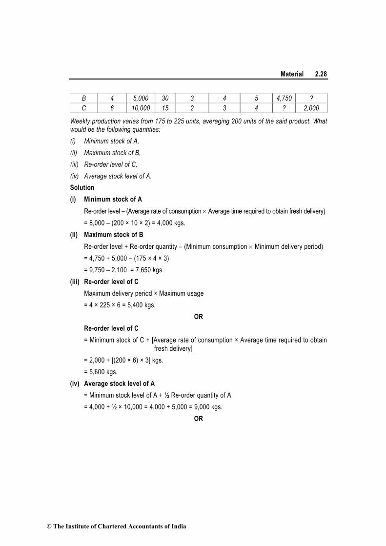
Material 2.28
B 4 5,000 30 3 4 5 4,750 ?
C 6 10,000 15 2 3 4 ? 2,000
Weekly production varies from 175 to 225 units, averaging 200 units of the said product. What would be the following quantities:
(i) Minimum stock of A,
(ii) Maximum stock of B,
(iii) Re-order level of C,
(iv) Average stock level of A.
Solution
(i) Minimum stock of A
Re-order level – (Average rate of consumption Average time required to obtain fresh delivery)
= 8,000 – (200 × 10 × 2) = 4,000 kgs.
(ii) Maximum stock of B
Re-order level + Re-order quantity – (Minimum consumption Minimum delivery period)
= 4,750 + 5,000 – (175 × 4 × 3)
= 9,750 – 2,100 = 7,650 kgs.
(iii) Re-order level of C
Maximum delivery period × Maximum usage
= 4 × 225 × 6 = 5,400 kgs.
OR
Re-order level of C
= Minimum stock of C + [Average rate of consumption × Average time required to obtain
fresh delivery]
= 2,000 + [(200 × 6) × 3] kgs.
= 5,600 kgs.
(iv) Average stock level of A
= Minimum stock level of A + ½ Re-order quantity of A
= 4,000 + ½ × 10,000 = 4,000 + 5,000 = 9,000 kgs.
OR
© The Institute of Chartered Accountants of India

2.29 Cost Accounting
Average Stock level of A
Minimum stock level of A Maximum stock level of A
2
(Refer to working note)
4,000 16,250
2
= 10,125 kgs.
Working note:
Maximum stock of A = ROL+ ROQ – (Minimum consumption Minimum re-order period)
= 8,000 + 10,000 – [(175 10) 1]
= 16,250 kgs.
Illustration 10: (Evaluation of discount offer and EOQ)
(a) EXE Limited has received an offer of quantity discounts on its order of materials as under:
Price per tonne (`) Tonnes (Nos.)
1,200 Less than 500
1,180 500 and less than 1,000
1,160 1,000 and less than 2,000
1,140 2,000 and less than 3,000
1,120 3,000 and above.
The annual requirement for the material is 5,000 tonnes. The ordering cost per order is
` 1,200 and the stock holding cost is estimated at 20% of material cost per annum. You
are required to compute the most economical purchase level.
(b) What will be your answer to the above question if there are no discounts offered and the
price per tonne is ` 1,500?
Solution
(a)
Total annual requirement
(A)
Order size
(Tonne)
(q)
No. of orders
A/q
Cost of inventory
A Per tonne cost
(`)
Ordering cost
A/q `1200
(`)
Carrying cost
p.t.p.a
1/2 q 20% of cost p.t.(`)
Total Cost (4+5+6)
(`)
1 2 3 4 5 6 7
5,000 tonne 400 12.5 60,00,000 15,000 48,000 60,63,000
(5,000`1200) (200 ` 240)
500 10 59,00,000 12,000 59,000 59,71000
(5,000` 1180) (250 ` 236)
© The Institute of Chartered Accountants of India

Material 2.30
1,000 5 58,00,000 6,000 1,16,000 59,22,000
(5,000` 1160) (500 ` 232)
2,000 2.5 57,00,000 3,000 2,28,000 59,31,000
(5,000` 1140) (1,000`228)
3,000 1.666 56,00,000 2,000 3,36,000 59,38,000
(5,000` 1120) (1,500`224)
The above table shows that the total cost of 5,000 units including ordering and carrying
cost is minimum (` 59,22,000) when the order size is 1,000 units. Hence the most
economical purchase level is 1,000 units.
(b) If there will are no discount offer then the purchase quantity should be equal to EOQ. The
EOQ is as follows:
EOQ = 2AO
C
where A is the annual inventory requirement,
O is the ordering cost per order and
C is the carrying cost per unit per annum.
=
2 5,000 units 1,200200 units
20% 1,500
`
`
Illustration 11: (Calculation of Stock Levels and Danger level)
From the details given below, calculate:
(i) Re-ordering level
(ii) Maximum level
(iii) Minimum level
(iv) Danger level.
Re-ordering quantity is to be calculated on the basis of following information:
Cost of placing a purchase order is ` 20
Number of units to be purchased during the year is 5,000
Purchase price per unit inclusive of transportation cost is ` 50
Annual cost of storage per units is ` 5.
Details of lead time : Average- 10 days, Maximum- 15 days, Minimum- 5 days.
For emergency purchases- 4 days.
© The Institute of Chartered Accountants of India

2.31 Cost Accounting
Rate of consumption : Average: 15 units per day,
Maximum: 20 units per day.
Solution
Basic Data:
A (Number of units to be purchased annually) = 5,000 units
O (Ordering cost per order) = ` 20
C (Annual cost of storage per unit) = ` 5
Purchase price per unit inclusive of transportation cost = ` 50.
Computations:
(i) Re-ordering level = Maximum usage per period × Maximum lead time
(ROL) = 20 units per day × 15 days = 300 units
(ii) Maximum level = ROL + ROQ – [Min. rate of consumption × Min. lead time]
(Refer to working notes1 and 2)
= 300 units + 200 units – [10 units per day × 5 days] = 450 units
(iii) Minimum level = ROL – Average rate of consumption × Average re-order-period
= 300 units – (15 units per day × 10 days) =150 units
(iv) Danger level = Average consumption × Lead time for emergency purchases
= 15 units per day × 4 days = 60 units
Working Notes:
1. Minimum rate of consumption per day
Minimum rate of Maximum rate of
Av. rate of consumption consumption
consumption 2
15 units per day = X units / day 20 units per day
2
or X = 10 units per day.
2. Re-order Quantity (ROQ)
= 2 5,000 units 20
200 units5
Illustration 12: (EOQ and calculation of minimum carrying cost)
G. Ltd. produces a product which has a monthly demand of 4,000 units. The product requires
a component X which is purchased at ` 20. For every finished product, one unit of component
© The Institute of Chartered Accountants of India

Material 2.32
is required. The ordering cost is ` 120 per order and the holding cost is 10% p.a.
You are required to calculate:
(i) Economic order quantity.
(ii) If the minimum lot size to be supplied is 4,000 units, what is the extra cost, the company
has to incur?
(iii) What is the minimum carrying cost, the company has to incur?
Solution
(a) (i) Economic order quantity:
A (Annual requirement or Component ‘X’) = 4,000 units per month × 12 months
= 48,000 units
C (Purchase cost p.u.) = ` 20
O (Ordering cost per order) = ` 120
i (Holding cost) = 10% per annum
E.O.Q. = 2AO
Ci
=2 48,000units 120
10% of 20
`
` = 2,400 units
(ii) Extra cost incurred by the company:
A. Total cost when order size is equal 4,000 units:
Total cost = Total ordering cost + Total carrying cost
= A
Q× O +
1
2Q (Ci)
= (units 000,4
units 000,48× ` 120) + (
2
1 × 4,000 units × 10% × ` 20)
= ` 1,440 + ` 4,000 = ` 5,440
B. Total cost when order size is equal EOQ i.e. 2,400 units:
Total cost = (units 400,2
units 000,48× ` 120) + (
2
1× 2,400 units × 10% × ` 20)
= ` 2,400 + ` 2,400 = ` 4,800
Extra cost that the company has to incur = (A) – (B) = ` 5,440 – ` 4,800 = ` 640
(iii) Minimum carrying cost :
Carrying cost depends upon the size of the order. It will be minimum on the least
order size. (In this part of the question the two order sizes are 2,400 units and 4,000
© The Institute of Chartered Accountants of India

2.33 Cost Accounting
units. Here 2,400 units is the least of the two order sizes. At this order size carrying
cost will be minimum.)
The minimum carrying cost in this case can be computed as under :
Minimum carrying cost = 2
1× 2,400 units × 10% × ` 20 = ` 2,400.
Illustration 13: (Calculation of Stock out Cost)
M/s Tyrotubes trades in four wheeler tyres and tubes. It stocks sufficient quantity of tyres of almost
every vehicle. In year end 20X1-X2, the report of sales manager revealed that
M/s Tyrotubes experienced stock-out of tyres.
The stock-out data is as follows:
Stock-out of Tyres* No. of times
100 2
80 5
50 10
20 20
10 30
0 33
M/s Tyrotubes loses `150 per unit due to stock-out and spends ` 50 per unit on carrying of
inventory.
Determine optimum safest stock level.
*Demand that could not be fulfilled due to insufficient stock of tyres.
Solution: Computation of Stock-out and Inventory carrying cost
Safety Stock Level (units)
(1)
Stock-out (units)
(2)
Probability
(3)
Stock-out cost(`)
(4)=(2) x `150
Expected stock-out
cost(`)
(5)=(3)x(4)
Inventory carrying cost
(`)
(6)=(1)x`50
Total cost (`)
(7)=(5)+(6)
100 0 0.00 0 0 5,000 5,000
80 20 0.02 3,000 60 4,000 4,060
50 50
30
0.02
0.05
7,500
4,500
150
225
12,000 375 2,500 2,875
20 80
60
30
0.02
0.05
0.10
12,000
9,000
4,500
240
450
450
© The Institute of Chartered Accountants of India

Material 2.34
25,500 1,140 1,000 2,140
10 90
70
40
10
0.02
0.05
0.10
0.20
13,500
10,500
6,000
1,500
270
525
600
300
31,500 1,695 500 2,195
0 100
80
50
20
10
0.02
0.05
0.10
0.20
0.30
15,000
12,000
7,500
3,000
1,500
300
600
750
600
450
2,700
39,000 2,700 0 2,700
At safety stock level of 20 units, total cost is least i.e. ` 2,140.
Working Note: Computation of Probability of Stock-out
Stock-out (units) 100 80 50 20 10 0 Total
Nos. of times 2 5 10 20 30 33 100
Probability 0.02 0.05 0.10 0.20 0.30 0.33 1.00
Explanation:
Stock-out means the demand of an item that could not be fulfilled because of insufficient stock level.
Safety stock is the level of stock of any item which is maintained in excess of lead time consumption. It is kept as cushion against any unexpected demand for that item.
Safety stock level Impact
100 units Any unexpected demand upto 100 units can be met.
80 units Stock out will only arise if unexpected demand will be for 100 units. In this case 20 units will remain unsatisfied. The probability of any unexpected demand for 100 units is 0.02.
50 units Any unexpected demand beyond 50 units will be remain unsatisfied. If unexpected demand for 100 units arises (probability is 0.02) 50 units will be unsatisfied. Similarly if unexpected demand for 80 units arises (probability is 0.05), 30 units will be unsatisfied.
20 units Any unexpected demand beyond 20 units will be remain unsatisfied. If unexpected demand for 100 units arises (probability is 0.02), 80 units will remain unsatisfied. If unexpected demand for 80 units arises (probability is 0.05), 60 units will remain unsatisfied. Similarly, when unexpected demand for 50 units arises (probability is 0.10), 30 units will remain unsatisfied.
10 units Any unexpected demand beyond 10 units will be remain unsatisfied. If unexpected demand for 100 units arises (probability is 0.02), 90 units will remain unsatisfied. If unexpected demand for 80 units arises (probability is
© The Institute of Chartered Accountants of India

2.35 Cost Accounting
0.05), 70 units will remain unsatisfied. If unexpected demand for 50 units arises (probability is 0.10), 40 units will remain unsatisfied. Similarly, when unexpected demand for 20 units arises (probability is 0.20), 10 units will remain unsatisfied.
0 unit When no safety stock level is maintained, any unexpected demand cannot be satisfied. If unexpected demand for 100 units arises (probability is 0.02), 100 units will remain unsatisfied. If unexpected demand for 80 units arises (probability is 0.05), 80 units will remain unsatisfied. If unexpected demand for 50 units arises (probability is 0.10), 50 units will remain unsatisfied. If unexpected demand for 20 units arises (probability is 0.20), 20 units will remain unsatisfied. Similarly, unexpected demand for 10 units (probability is 0.30), 10 units will remain unsatisfied.
2.6.2 Techniques of Inventory Control: Depending on the type of organization and type of inventory specific inventory control techniques are adopted. Some of these are:
(1) ABC Analysis: This system exercises discriminating control over different items of stores
classified on the basis of the investment involved. Usually the items are divided into three
categories according to their importance, namely, their value and frequency of
replenishment during a period.
(i) ‘A’ Category of items consists of only a small percentage i.e., about 10% of the total
items handled by the stores but require heavy investment about 70% of inventory
value, because of their high prices or heavy requirement or both. Items under this
category can be controlled effectively by using a regular system which ensures
neither over-stocking nor shortage of materials for production. Such a system plans
its total material requirements by making budgets. The stocks of materials are
controlled by fixing certain levels like maximum level, minimum level and re-order
level.
(ii) ‘B’ Category of items are relatively less important; they may be 20% of the total
items of material handled by stores. The percentage of investment required is about
20% of the total investment in inventories. In the case these items, as the sum
involved is moderate, the same degree of control as applied in ‘A’ category of items
is not warranted. The orders for the items, belonging to this category may be placed
after reviewing their situation periodically.
(iii) ‘C’ Category of items do not require much investment; it may be about 10% of total
inventory value but they are nearly 70% of the total items handled by store. For
these category of items, there is no need of exercising constant control. Orders for
items in this group may be placed either after six months or once in a year, after
ascertaining consumption requirements. In this case the objective is to economies
on ordering and handling costs.
© The Institute of Chartered Accountants of India

Material 2.36
Illustration 14: (Application of ABC inventory control system)
A factory uses 4,000 varieties of inventory. In terms of inventory holding and inventory usage,
the following information is compiled:
No. of varieties % % value of inventory % of inventory usage of inventory holding (average) (in end-product)
3,875 96.875 20 5 110 2.750 30 10 15 0.375 50 85
4,000 100.000 100 100
Classify the items of inventory as per ABC analysis with reasons.
Solution
Classification of the items of inventory as per ABC analysis
1. 15 number of varieties of inventory items should be classified as ‘A’ category items
because of the following reasons:
(i) Constitute 0.375% of total number of varieties of inventory handled by stores of
factory, which is minimum as per given classification in the table.
(ii) 50% of total use value of inventory holding (average) which is maximum according
to the given table.
(iii) Highest in consumption about 85% of inventory usage (in end-product).
© The Institute of Chartered Accountants of India

2.37 Cost Accounting
2. 110 number of varieties of inventory items should be classified as ‘B’ category items
because of the following reasons:
(i) Constitute 2.750% of total number of varieties of inventory items handled by stores
of factory.
(ii) Requires moderate investment of about 30% of total use value of inventory holding
(average).
(iii) Moderate in consumption about 10% of inventory usage (in end–product).
3. 3,875 number of varieties of inventory items should be classified as ‘C’ category items
because of the following reasons:
(i) Constitute 96.875% of total varieties of inventory items handled by stores of factory.
(ii) Requires about 20% of total use value of inventory holding (average).
(iii) Minimum inventory consumption i.e. about 5% of inventory usage (in end-product).
Illustration 15: (Application of ABC in inventory control system)
From the following details, draw a plan of ABC selective control:
Item Units Unit cost (`)
1 7,000 5.00
2 24,000 3.00
3 1,500 10.00
4 600 22.00
5 38,000 1.50
6 40,000 0.50
7 60,000 0.20
8 3,000 3.50
9 300 8.00
10 29,000 0.40
11 11,500 7.10
12 4,100 6.20
Solution
Statement of Total Cost and Ranking
Item Units %of Total units
Unit cost (`)
Total cost (`) %of Total cost Ranking
1 7,000 3.1963 5.00 35,000 9.8378 4
2 24,000 10.9589 3.00 72,000 20.2378 2
3 1,500 0.6849 10.00 15,000 4.2162 7
© The Institute of Chartered Accountants of India

Material 2.38
4 600 0.2740 22.00 13,200 3.7103 8
5 38,000 17.3516 1.50 57,000 16.0216 3
6 40,000 18.2648 0.50 20,000 5.6216 6
7 60,000 27.3973 0.20 12,000 3.3730 9
8 3,000 1.3699 3.50 10,500 2.9513 11
9 300 0.1370 8.00 2,400 0.6746 12
10 29,000 13.2420 0.40 11,600 3.2605 10
11 11,500 5.2512 7.10 81,650 22.9502 1
12 4,100 1.8721 6.20 25,420 7.1451 5
2,19,000 100 3,55,770 100
Basis for selective control (Assumed)
` 50,000 & above -- ‘A’ items
` 15,000 to 50000 -- ‘B’ items
Below ` 15,000 -- ‘C’ items
On this basis, a plan of A B C selective control is given below:
Ranking Item Nos. % of Total units Cost (`) % of Total Cost Category
1 11 5.2512 81,650 22.9502
2 2 10.9589 72,000 20.2378
3 5 17.3516 57,000 16.0216
Total 3 33.5617 2,10,650 59.2096 A
4 1 3.1963 35,000 9.8378
5 12 1.8721 25,420 7.1451
6 6 18.2648 20,000 5.6216
7 3 0.6849 15,000 4.2162
Total 4 24.0181 95,420 26.8207 B
8 4 0.2740 13,200 3.7103
9 7 27.3973 12,000 3.3730
10 10 13.2420 11,600 3.2605
11 8 1.3699 10,500 2.9513
12 9 0.1370 2,400 0.6746
Total 5 42.4202 49,700 13.9697 C
Grand Total 12 100 3,55,770 100
© The Institute of Chartered Accountants of India

2.39 Cost Accounting
(1) Advantages of ABC analysis: The advantages of ABC analysis are the following :
(i) Continuity in production: It ensures that, without there being any danger of
interruption of production for want of materials or stores, minimum investment will
be made in inventories of stocks of materials or stocks to be carried.
(ii) Lower cost: The cost of placing orders, receiving goods and maintaining stocks is
minimised specially if the system is coupled with the determination of proper
economic order quantities.
(iii) Less attention required: Management time is saved since attention need be paid
only to some of the items rather than all the items as would be the case if the ABC
system was not in operation.
(iv) Systematic working: With the introduction of the ABC system, much of the work
connected with purchases can be systematized on a routine basis to be handled by
subordinate staff.
(2) HML: In this system inventory items are classified as high price, medium price and low
cost items.
(3) VED: Items are classified as vital, essential and desirable items under this system. This
system is used particularly in spare parts inventory.
(4) FSN: Items are classified as fast moving, slow moving and non-moving items.
(5) GOLF: This system is based on sources of items. These are classified as Government
supply, ordinary supply, local and foreign supply.
(6) SOS: Items are classified as seasonal and off seasonal items.
2.6.3 Two Bin System: Under this system each bin is divided into two parts - one, smaller part,
should stock the quantity equal to the minimum stock or even the re-ordering level, and the other to
keep the remaining quantity. Issues are made out of the larger part; but as soon as it becomes
necessary to use quantity out of the smaller part of the bin, fresh order is placed. “Two Bin System”
is supplemental to the record of respective quantities on the bin card and the stores ledger card.
2.6.4 Establishment of system of budgets: To control investment in the inventories, it is necessary to know in advance about the inventories requirement during a specific period usually a year. The exact quantity of various types of inventories and the time when they would be required can be known by studying carefully production plans and production schedules. Based on this, inventories requirement budget can be prepared. Such a budget will discourage the unnecessary investment in inventories.
2.6.5 Use of perpetual inventory records and continuous stock verification: Perpetual inventory represents a system of records maintained by the stores department. It in fact comprises: (i) Bin Cards, and (ii) Stores Ledger.
The success of perpetual inventory depends upon the following:
(a) The Stores Ledger(showing quantities and amount of each item).
© The Institute of Chartered Accountants of India

Material 2.40
(b) Stock Control cards (or Bin Cards).
(c) Reconciling the quantity balances shown by (a) & (b) above.
(d) Checking the physical balances of a number of items every day systematically and by
rotation.
(e) Explaining promptly the causes of discrepancies, if any, between physical balances and
book figures.
(f) Making corrective entries where called for after step (e) and
(g) Removing the causes of the discrepancies referred to in step (e)
Advantages of perpetual inventory: The main advantages of perpetual inventory are as
follows:
(1) Physical stocks can be counted and book balances adjusted as and when desired
without waiting for the entire stock-taking to be done.
(2) Quick compilation of Profit and Loss Account (for interim period) due to prompt
availability of stock figures.
(3) Discrepancies are easily located and thus corrective action can be promptly taken to
avoid their recurrence.
(4) A systematic review of the perpetual inventory reveals the existence of surplus, dormant,
obsolete and slow-moving materials, so that remedial measures may be taken in time.
(5) Fixation of the various stock levels and checking of actual balances in hand with these
levels assist the Store keeper in maintaining stocks within limits and in initiating purchase
requisitions for correct quantity at the proper time.
Continuous Stock Verification The checking of physical inventory is an essential feature
of every sound system of material control. Such a checking may be periodical or continuous.
Moreover, in the case of periodical checking there is the problem of finding an adequately
trained contingent. It is likely to be drawn from different departments where stock-taking is not
the normal work and they are apt to discharge such temporary duties somewhat perfunctorily.
The element of surprise, that is essential for effective control is wholly absent in the system.
Then if there are stock discrepancies, they remain undetected until the end of the period.
Often, the discrepancies are not corrected.
The system of continuous stock-taking consists of counting and verifying the number of items
daily throughout the year so that during the year all items of stores are covered three or four
times. The stock verifiers are independent of the stores, and the stores staffs have no
foreknowledge as to the particular items that would be checked on any particular day. But it
must be seen that each item is checked a number of times in a year.
Advantages of continuous stock-taking: The advantages of continuous stock-taking are:
1. Closure of normal functioning is not necessary.
© The Institute of Chartered Accountants of India
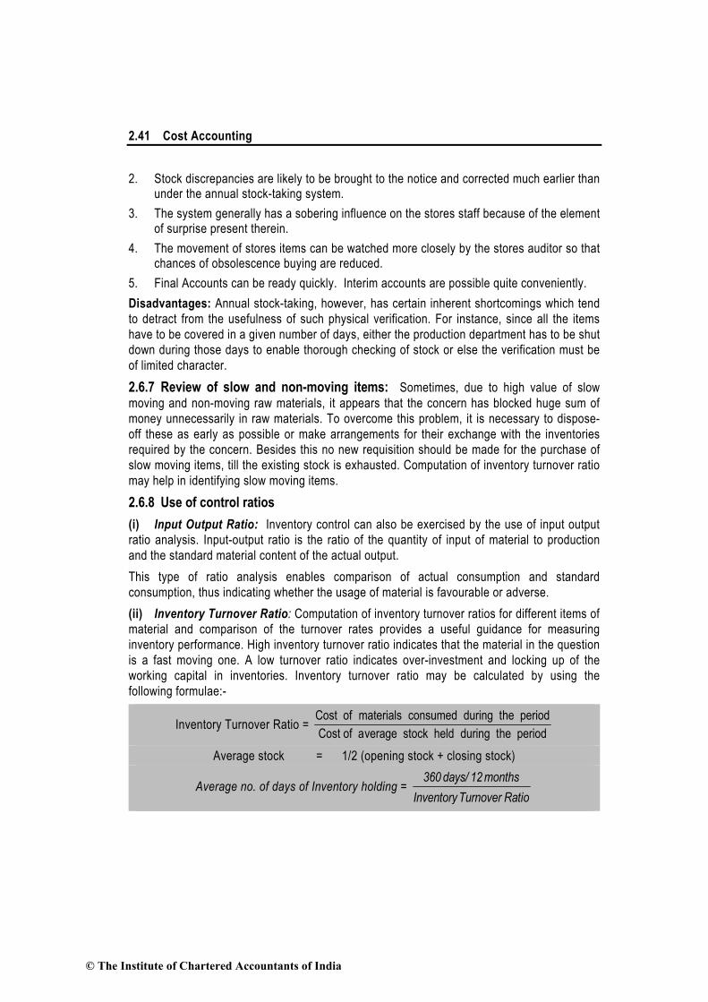
2.41 Cost Accounting
2. Stock discrepancies are likely to be brought to the notice and corrected much earlier than under the annual stock-taking system.
3. The system generally has a sobering influence on the stores staff because of the element of surprise present therein.
4. The movement of stores items can be watched more closely by the stores auditor so that chances of obsolescence buying are reduced.
5. Final Accounts can be ready quickly. Interim accounts are possible quite conveniently.
Disadvantages: Annual stock-taking, however, has certain inherent shortcomings which tend
to detract from the usefulness of such physical verification. For instance, since all the items
have to be covered in a given number of days, either the production department has to be shut
down during those days to enable thorough checking of stock or else the verification must be
of limited character.
2.6.7 Review of slow and non-moving items: Sometimes, due to high value of slow
moving and non-moving raw materials, it appears that the concern has blocked huge sum of
money unnecessarily in raw materials. To overcome this problem, it is necessary to dispose-
off these as early as possible or make arrangements for their exchange with the inventories
required by the concern. Besides this no new requisition should be made for the purchase of
slow moving items, till the existing stock is exhausted. Computation of inventory turnover ratio
may help in identifying slow moving items.
2.6.8 Use of control ratios
(i) Input Output Ratio: Inventory control can also be exercised by the use of input output
ratio analysis. Input-output ratio is the ratio of the quantity of input of material to production
and the standard material content of the actual output.
This type of ratio analysis enables comparison of actual consumption and standard
consumption, thus indicating whether the usage of material is favourable or adverse.
(ii) Inventory Turnover Ratio: Computation of inventory turnover ratios for different items of
material and comparison of the turnover rates provides a useful guidance for measuring
inventory performance. High inventory turnover ratio indicates that the material in the question
is a fast moving one. A low turnover ratio indicates over-investment and locking up of the
working capital in inventories. Inventory turnover ratio may be calculated by using the
following formulae:-
Inventory Turnover Ratio = he period during tock held verage stCost of a
he period during t consumed materials Cost of
Average stock = 1/2 (opening stock + closing stock)
Average no. of days of Inventory holding = 360 days/ 12 months
Inventory Turnover Ratio
© The Institute of Chartered Accountants of India

Material 2.42
By comparing the number of days in the case of two different materials, it is possible to know which is fast moving and which is slow moving. On this basis, attempt should be made to reduce the amount of capital locked up, and prevent over-stocking of the slow moving items.
Illustration 16: (Calculation of inventory turnover ratio)
The following data are available in respect of material X for the year ended 31st March, 20X1.
(`) Opening stock 90,000
Purchases during the year 2,70,000
Closing stock 1,10,000
Calculate:
(i) Inventory turnover ratio, and
(ii) The number of days for which the average inventory is held.
Solution
Inventory turnover ratio
(Refer to working note) = material raw of stock Average
consumed material raw of stock ofCost
= `
`
2,50,000
1,00,000= 2.5
Average number of days for which
the average inventory is held = ratio turnoverInventory
365=
5.2
days365 = 146 days
Working Note: (`)
Opening stock of raw material 90,000
Add: Material purchases during the year 2,70,000
Less: Closing stock of raw material 1,10,000
Cost of stock of raw material consumed 2,50,000
Illustration 17: (Calculation of inventory turnover ratio)
From the following data for the year ended 31st December, 20X1, calculate the inventory turnover ratio of the two items and put forward your comments on them.
Material A (`) Material B(`)
Opening stock 1.1.20X1 10,000 9,000
Purchase during the year 52,000 27,000
Closing stock 31.12.20X1 6,000 11,000
© The Institute of Chartered Accountants of India

2.43 Cost Accounting
Solution
First of all it is necessary to find out the material consumed:
Cost of materials consumed Material A Material B
(`) (`)
Opening stock 10,000 9,000
Add: Purchases 52,000 27,000
62,000 36,000
Less: Closing stock 6,000 11,000
Materials consumed 56,000 25,000
Average inventory: (Opening Stock + Closing Stock) 2 8,000 10,000
Inventory Turnover ratio: (Consumption Average inventory) 7 times 2.5 times
Inventory Turnover (Number of Days in a year/IT ratio) 52 days 146 days
Comments: Material A is moving faster than Material B.
2.7 Material Issue Procedure
Issue of material must not be made except under properly authorised requisition slip; usually it
is the foreman of a department who has the authority to draw materials from the store. Issue
of material must be made on the basis of first in first out, that is, out of the earliest lot on hand.
If care is not exercised in this regard, quality of earliest lot of material may deteriorate for
having been kept for a long period.
Material Requisition Note: It is the voucher of the authority as regards issue of materials for
use in the factory or in any of its departments. After receipt of material requisition slip store
keeper ensures that requisition is properly authorized and requisitioned quantity is within the
quantity specified in bill of materials. After satisfied with the documents, store keeper issue
materials and keep one copy of based materials and record the transaction in the records
maintained by the stores department.
Transfer of Material: The surplus material arising on a job or other units of production may
sometime be unsuitable for transfer to Stores because of its bulk, heavy weight, brittleness or
some such reason. It may, however, be possible to find some alternative use for such
materials by transferring it to some other job instead of returning it to the Store Room.
It must be stressed that generally transfer of material from one job to another is irregular, if not
improper, in so far it is not conducive to correct allocation and control of material cost of jobs
or other units of production. It is only in the circumstances envisaged above that such direct
transfer should be made, at the time of material transfer a material transfer note should be
made in duplicate, the disposition of the copies of this note being are as follows :
© The Institute of Chartered Accountants of India

Material 2.44
Material Transfer Note
Cost Department Department Making Transfer
No copy is required for the Store as no entry in the stores records would be called for. The
Cost Department would use its copy for the purpose of making the necessary entries in the
cost ledger accounts for the jobs affected.
The form of the Material Transfer Note is shown below:
Material Transfer Note
From Job No. .................................. No. ....................................
To Job No. ........................................ Date .................................
Item No. Particulars Rate Amount
` `
Transferred by Received by ....................................
Job Ledger Clerk
Return of Material: Sometimes, it is not possible before hand to make any precise estimate of the material requirements or units of production. Besides, at times due to some technical or other difficulty, it is not practicable to measure exactly the quantity of material required by a department. In either case, material may have to be issued from stores in bulk, often in excess of the actual quantity required. Where such a condition exists, it is of the utmost importance from the point of view of materials control that any surplus material left over on the completion of a job should be promptly hand over to the storekeeper for safe and proper custody.
Unless this is done, the surplus material may be misappropriated or misapplied to some purpose, other than that for which it was intended. The material cost of the job against which the excess material was originally drawn in that case, would be overstated unless the job is given credit for the surplus arising thereon.
The surplus material, when it is returned to the storeroom, should be accompanied by a document known either as a Shop Credit Note or alternatively as a Stores Debit Note. This document should be made out, by the department returning the surplus material and it should be in triplicate to be used as follows:
Shop Credit Note
Store Room Cost Department Department Returning it
© The Institute of Chartered Accountants of India

2.45 Cost Accounting
The form of Shop Credit Note is given below:
Shop Credit Note
Job No. ...................................... No. ........................
Department ............................ Date ......................
Item No. Particulars Qnty. Rate Amount
Store-keeper S.L. Clerk Foreman of the Returning Department
2.8 Valuation of Material Issues
Materials issued from stores should be priced at the value at which they are carried in stock.
But there can be a situation where the material may have been purchased at different times
and at different prices with varying discounts, taxes etc. Because of this the problem arises as
to how the material issues to production are to be valued. There are several methods for
tackling this situation. The cost accountant should select the proper method based on
following factors:
1. The frequency of purchases, price fluctuations and its range.
2. The frequency of issue of materials, relative quantity etc.
3. Nature of cost accounting system.
4. The nature of business and type of production process.
5. Management policy relating to valuation of closing stock.
Several methods of pricing material issues have been evolved in an attempt to satisfactorily answer the problem. These methods may be grouped and explained as follows:
2.8.1 Cost Price Methods:
(a) Specific price method.
(b) First-in First-out method.
(c) Last-in-First-out method.
(d) Base stock method.
2.8.2 Average Price Methods:
(e) Simple average price method.
(f) Weighted average price method.
(g) Periodic simple average price method.
(h) Periodic weighted average price method.
© The Institute of Chartered Accountants of India

Material 2.46
(i) Moving simple average price method.
(j) Moving weighted average price method.
2.8.3 Market Price Methods:
(k) Replacement price method.
(l) Realisable price method.
2.8.4 Notional Price Methods:
(m) Standard price method.
(n) Inflated price methods.
(o) Re-use Price Method.
We may now briefly discuss all the above methods:
(a) Specific Price Method
Meaning Suitability
This method is useful, specially when materials are purchased for a specific job or work order, and as such these materials are issued subsequently to that specific job or work order at the price at which they were purchased.
To use this method, it is necessary to store each lot of material separately and maintain its separate account.
Advantages and disadvantages
Advantages Disadvantages
The cost of materials issued for production purposes to specific jobs represent actual and correct costs.
This method is difficult to operate, specially when purchases and issues are numerous.
This method is best suited for non-standard and specific products.
(b) First-in-First out Method (FIFO)
Meaning Suitability
It is a method of pricing the issues of materials, in the order in which they are purchased. In other words, the materials are issued in the order in which they arrive in the store or the items longest in stock are issued first. Thus each issue of material only recovers the purchase price which does not reflect the current market price.
This method is considered suitable in times of falling price because the material cost charged to production will be high while the replacement cost of materials will be low. But, in the case of rising prices, if this method is adopted, the charge to production will be low as compared to the replacement cost of materials. Consequently, it would be difficult to purchase the same volume of material (as in the current period) in future without having additional capital resources.
© The Institute of Chartered Accountants of India

2.47 Cost Accounting
Advantages and disadvantages
Advantages Disadvantages
It is simple to understand and easy to operate.
If the prices fluctuate frequently, this method may lead to clerical error.
Material cost charged to production represents actual cost with which the cost of production should have been charged.
Since each issue of material to production is related to a specific purchase price, the costs charged to the same job are likely to show a variation from period to period.
In the case of falling prices, the use of this method gives better results.
In the case of rising prices, the real profits of the concern being low, they may be inadequate to meet the concern’s demand to purchase raw materials at the ruling price.
Closing stock of material will be represented very closely at current market price.
The application of FIFO method is illustrated below:
Material Received and Issued
Lot No.
Date Quantity Kg.
Lot No.
Rate (`)
Amount (`)
1. July 3 600 1.00 600.00
2. July 13 800 1.20 960.00
3. July 23 600 0.90 540.00
4. August 5 400 1.10 440.00
5. August 6 1200 0.80 960.00
July 8 400 Kgs. out of (1) 1.00 400.00
July 12 200 Kgs. out of (1) 1.00 200.00
July 22 600 Kgs. out of (2) 1.20 720.00
July 25 200 Kgs. out of (2) 1.20 240.00
200 Kgs. out of (3) 0.90 180.00
August 8 400 Kgs. out of (3) 0.90 360.00
400 Kgs. out of (4) 1.10 440.00
200 Kgs. out of (5) 0.80 160.00
The stock in hand after 8th August will be 1,000 Kgs. This will be out of lot number (5) and its value will be ` 800, i.e., @ ` 0.80 per Kg.
© The Institute of Chartered Accountants of India

Material 2.48
(c) Last-in-First out method (LIFO)
Meaning Suitability
It is a method of pricing the issues of materials. This method is based on the assumption that the items of the last batch (lot) purchased are the first to be issued. Therefore, under this method the prices of the last batch (lot) are used for pricing the issues, until it is exhausted, and so on. If however, the quantity of issue is more than the quantity of the latest lot than earlier (lot) and its price will also be taken into consideration.
During inflationary period or period of rising prices, the use of LIFO would help to ensure that the cost of production determined on the above basis is approximately the current one. This method is also useful specially when there is a feeling that due to the use of FIFO or average methods, the profits shown and tax paid are too high.
Advantages and Disadvantages
Advantages Disadvantages
The cost of materials issued will be either nearer to and or will reflect the current market price. Thus, the cost of goods produced will be related to the trend of the market price of materials. Such a trend in price of materials enables the matching of cost of production with current sales revenues.
Calculation under LIFO system becomes complicated and cumbersome when frequent purchases are made at highly fluctuating rates.
The use of the method during the period of rising prices does not reflect undue high profit in the income statement as it was under the first-in-first-out or average method. In fact, the profit shown here is relatively lower because the cost of production takes into account the rising trend of material prices.
Costs of different similar batches of production carried on at the same time may differ a great deal.
In the case of falling prices profit tends to rise due to lower material cost, yet the finished products appear to be more competitive and are at market price.
In time of falling prices, there will be need for writing off stock value considerably to stick to the principle of stock valuation, i.e., the cost or the market price whichever is lower.
Over a period, the use of LIFO helps to iron out the fluctuations in profits.
This method of valuation of material is not acceptable to the income tax authorities.
© The Institute of Chartered Accountants of India

2.49 Cost Accounting
In the period of inflation LIFO will tend to show the correct profit and thus avoid paying undue taxes to some extent.
It may be noted that Last in First out (LIFO) is not permitted under Accounting
Standard (AS)-2: Valuation of Inventories. However for the purpose of academic
knowledge LIFO method is included in this Study Material.
(d) Base Stock Method
Meaning Suitability
Minimum quantity of stock under this method is always held at a fixed price as reserve in the stock, to meet a state of emergency, if it arises. This minimum stock is known as base stock and is valued at a price at which the first lot of materials is received and remains unaffected by subsequent price fluctuations.
This method of valuing inventory than a method of valuing issues because, with the base of stock valued at the original cost some other method of valuing issues should be adopted. The quantity in excess of the base stock may be valued either on the FIFO or LIFO basis. This method is not an independent method as it uses FIFO or LIFO. Its advantages and disadvantages therefore will depend upon the use of the other method viz., FIFO or LIFO.
Illustration 18: (Treatment of shortage in stock taking)
‘AT’ Ltd. furnishes the following store transactions for September, 2011 :
1-9-11 Opening balance 25 units value ` 162.50
4-9-11 Issues Req. No. 85 8 units
6-9-11 Receipts from B & Co. GRN No. 26 50 units @ ` 5.75 per unit
7-9-11 Issues Req. No. 97 12 units
10-9-11 Return to B & Co. 10 units
12-9-11 Issues Req. No. 108 15 units
13-9-11 Issues Req. No. 110 20 units
15-9-11 Receipts from M & Co. GRN. No. 33 25 units @ ` 6.10 per unit
17-9-11 Issues Req. No. 121 10 units
19-9-11 Received replacement from B & Co.
GRN No. 38 10 units
20-9-11 Returned from department, material of
M & Co. MRR No. 4 5 units
22-9-11 Transfer from Job 182 to Job 187 in the
© The Institute of Chartered Accountants of India

Material 2.50
dept. MTR 6 5 units
26-9-11 Issues Req. No. 146 10 units
29-9-11 Transfer from Dept. “A” to Dept. “B” MTR 10 5 units
30-9-11 Shortage in stock taking 2 units
Write up the priced stores ledger on FIFO method and discuss how would you treat the shortage in stock taking.
Solution
Working Notes:
1. The material received as replacement from vendor is treated as fresh supply.
2. In the absence of information the price of the material received from within on 20-9-11 has been taken as the price of the earlier issue made on 17-9-11. In FIFO method physical flow of the material is irrelevant for pricing the issues.
3. The issue of material on 26-9-11 is made out of the material received from within.
4. The entries for transfer of material from one job and department to other on 22-9-11 and 29-9-11 are book entries for adjusting the cost of respective jobs and as such they have not been shown in the stores ledger account.
5. The material found short as a result of stock taking has been written off.
© The Institute of Chartered Accountants of India

2.51 Cost Accounting
So
luti
on
:
Sto
res
Le
dg
er
of
AT
Ltd
. fo
r th
e m
on
th o
f S
ep
tem
be
r, 2
01
1 (
FIF
O M
eth
od
)
R
EC
EIP
T
ISS
UE
B
AL
AN
CE
Da
te
GR
N N
o.
Qty
. R
ate
A
mo
un
t R
eq
uis
i-
Qty
. R
ate
A
mo
un
t Q
ty.
Ra
te
Am
ou
nt
M
RR
No
. U
nit
s
(`)
(`)
tio
n N
o.
Un
its
(`
) (`
) U
nit
s
(`)
(`)
1
2
3
4
5
6
7
8
9
10
1
1
12
1-9
-11
—
—
—
—
—
—
—
—
2
5
6.5
0
16
2.5
0
4-9
-11
—
—
—
—
8
5
8
6.5
0
52
1
7
6.5
0
11
0.5
0
6-9
-11
2
6
50
5
.75
2
87
.50
—
—
—
—
1
7
6.5
0
5
0
5.7
5
39
8.0
0
7-9
-11
—
—
—
—
9
7
12
6
.50
7
8
5
6.5
0
5
0
5.7
5
32
0.0
0
10
-9-1
1
—
—
—
—
Nil
10
5
.75
5
7.5
0
5
6.5
0
4
0
5.7
5
26
2.0
0
12
-9-1
1
—
—
—
—
10
8
5
6.5
0
10
5
.75
9
0
30
5
.75
1
72
.50
13
-9-1
1
—
—
—
—
11
0
20
5
.75
1
15
1
0
5.7
5
57
.50
15
-9-1
1
33
2
5
6.1
0
15
2.5
0
—
—
—
—
10
5
.75
2
5
6.1
0
21
0.0
0
17
-9-1
1
—
—
—
—
12
1
10
5
.75
5
7.5
0
25
6
.10
1
52
.50
19
-9-1
1
38
1
0
5.7
5
57
.50
—
—
—
—
2
5
6.1
0
1
0
5.7
5
21
0.0
0
5
5
.75
20
-9-1
1
4
5
5.7
5
28
.75
—
—
—
—
2
5
6.1
0
25
8.7
5
1
0
7.7
5
26
-9-1
1
—
—
—
—
14
6
5
5.7
5
2
0
6.1
0
5
6.1
0
59
.25
1
0
5.7
5
17
9.5
0
30
-9-1
1
—
—
—
—
Sh
ort
ag
e
2
6.1
0
12
.20
1
8
6.1
0
1
0
5.7
5
16
7.3
0
© The Institute of Chartered Accountants of India

Material 2.52
Illustration 19: (Calculation of value of materials consumed and stock)
The following information is provided by Sunrise Industries for the fortnight of April, 2011:
Material Exe :
Stock on 1-4-2011 100 units at ` 5 per unit.
Purchases
5-4-11 300 units at ` 6
8-4-11 500 units at ` 7
12-4-11 600 units at ` 8
Issues
6-4-11 250 units
10-4-11 400 units
14-4-11 500 units
Required :
(A) Calculate using FIFO and LIFO methods of pricing issues :
(a) the value of materials consumed during the period
(b) the value of stock of materials on 15-4-11.
(B) Explain why the figures in (a) and (b) in part A of this question are different under the two
methods of pricing of material issues used. You need not draw up the Stores Ledgers.
Solution
(A) (a) Value of Material Exe consumed during the period
1-4-11 to 15-4-11 by using FIFO method.
Date Description Units Qty. (Units) Rate (`) Amount (`)
1-4-11 Opening balance 100 5 500
5-4-11 Purchased 300 6 1,800
6-4-11 Issued 100
150
6
5
1,400
8-4-11 Purchased 500 7 3,500
10-4-11 Issued 150
250
7
6
2,650
12-4-11 Purchased 600 8 4,800
14-4-11 Issued 250
250
8
7
3,750
15-4-11 Balance 350 8 2,800
© The Institute of Chartered Accountants of India

2.53 Cost Accounting
Total value of material Exe consumed during the period under FIFO method comes
to (` 1,400 + ` 2,650 + ` 3,750) ` 7,800 and balance on 15-4-11 is of ` 2,800.
Value of Material Exe consumed during the period
1-4-11 to 15-4-11 by using LIFO method
Date Description Qty. (Units) Rate (`) Amount (`)
1-4-11 Opening balance 100 5 500
5-4-11 Purchased 300 6 1,800
6-4-11 Issued 250 6 1,500
8-4-11 Purchased 500 7 3,500
10-4-11 Issued 400 7 2,800
12-4-11 Purchased 600 8 4,800
14-4-11 Issued 500 8 4,000
15-4-11 Balance 350 — 2,300*
Total value of material Exe issued under LIFO method comes to (` 1,500 + ` 2,800
+ ` 4,000) ` 8,300.
*The balance 350 units on 15-4-11 of ` 2,300, relates to opening balance on 1-4-11
and purchases made on 5-4-11, 8-4-11 and 12-4-11. (100 units @ ` 5, 50 units @ `
6, 100 units @ ` 7 and 100 units @ ` 8).
(b) As shown in (a) above, the value of stock of materials on 15-4-11:
Under FIFO method ` 2,800
Under LIFO method ` 2,300
(B) Total value of material Exe issued to production under FIFO and LIFO methods comes to
` 7,800 and ` 8,300 respectively. The value of closing stock of material Exe on 15-4-11
under FIFO and LIFO methods comes to ` 2,800 and ` 2,300 respectively.
The reasons for the difference of ` 500 (` 8,300 – ` 7,800) as shown by the following
table in the value of material Exe, issued to production under FIFO and LIFO are as
follows:
Date Quantity Value Total Value Total
Issued FIFO LIFO
(Units) (`) (`) (`) (`)
6-4-11 250 1,400 1,500
10-4-11 400 2,650 2,800
14-4-11 500 3,750 7,800 4,000 8,300
1. On 6-4-11, 250 units were issued to production. Under FIFO their value comes to
` 1,400 (100 units × ` 5 + 150 units × ` 6) and under LIFO ` 1,500 (250 × ` 6).
Hence, ` 100 was more charged to production under LIFO.
© The Institute of Chartered Accountants of India

Material 2.54
2. On 10-4-11, 400 units were issued to production. Under FIFO their value comes to
` 2,650 (150 × ` 6 + 250 × ` 7) and under LIFO ` 2,800 (400 × ` 7). Hence, ` 150
was more charged to production under LIFO.
3. On 14-4-11, 500 units were issued to production. Under FIFO their value comes to
` 3,750 (250 × ` 7 + 250 × ` 8) and under LIFO ` 4,000 (500 × ` 8). Hence, ` 250
was more charged to production under LIFO.
Thus the total excess amount charged to production under LIFO comes to ` 500.
The reasons for the difference of ` 500 (` 2,800 – ` 2,300) in the value of 350 units of
Closing Stock of material Exe under FIFO and LIFO are as follows :
1. In the case of FIFO, all the 350 units of the closing stock belongs to the purchase of
material made on 12-4-11, whereas under LIFO these units were from opening
balance and purchases made on 5-4-11, 8-4-11 and 12-4-11.
2. Due to different purchase price paid by the concern on different days of purchase,
the value of closing stock differed under FIFO and LIFO. Under FIFO 350 units of
closing stock were valued @ ` 8 p.u. Whereas under LIFO first 100 units were
valued @ ` 5 p.u., next 50 units @ ` 6 p.u., next 100 units @ ` 7 p.u. and last 100
units @ ` 8 p.u.
Thus under FIFO, the value of closing stock increased by ` 500.
Illustration 20: (Methods of pricing of materials)
The following transactions in respect of material Y occurred during the six months ended 30th
June, 2011:
Month Purchase (units) Price per unit Issued
(`) units
January 200 25 Nil
February 300 24 250
March 425 26 300
April 475 23 550
May 500 25 800
June 600 20 400
Required :
(a) The Chief Accountant argues that the value of closing stock remains the same no matter
which method of pricing of material issues is used. Do you agree? Why or why not?
Detailed stores ledgers are not required.
(b) When and why would you recommend the LIFO method of pricing material issues?
© The Institute of Chartered Accountants of India

2.55 Cost Accounting
Solution
(a) The Closing Stock at the end of six months period i.e., on 30th June, 2011 will be 200
units, whereas up to the end of May 2011, total purchases coincide with the total issues
i.e., 1,900 units. It means that at the end of May 2011, there was no closing stock. In the
month of June 2011, 600 units were purchased out of which 400 units were issued. Since
there was only one purchase and one issue in the month of June, 2011 and there was no
opening stock on 1st June 2011, the Closing Stock of 200 units is to be valued at ` 20
per unit.
In view of this, the argument of the Chief Accountant appears to be correct. Where there
is only one purchase and one issue in a month with no opening stock, the method of
pricing of material issues becomes irrelevant. Therefore, in the given case one should
agree with the argument of the Chief Accountant that the value of Closing Stock remains
the same no matter which method of pricing the issue is used.
It may, however, be noted that the argument of Chief Accountant would not stand if one
finds the value of the Closing Stock at the end of each month.
(b) LIFO method has an edge over FIFO or any other method of pricing material issues due
to the following advantages:
(i) The cost of the materials issued will be either nearer or will reflect the current
market price. Thus, the cost of goods produced will be related to the trend of the
market price of materials. Such a trend in price of materials enables the matching of
cost of production with current sales revenues.
(ii) The use of the method during the period of rising prices does not reflect undue high
profit in the income statement, as it was under the first-in-first-out or average
method. In fact, the profit shown here is relatively lower because the cost of
production takes into account the rising trend of material prices.
(iii) In the case of falling prices, profit tends to rise due to lower material cost, yet the
finished products appear to be more competitive and are at market price.
(iv) During the period of inflation, LIFO will tend to show the correct profit and thus,
avoid paying undue taxes to some extent.
(e) Simple Average Price Method
Meaning Suitability
Under this method, materials issued are valued at average price, which is calculated by dividing the total of all units rate by the number of unit rate.
1. When the materials are received in uniform lots of similar quantity, otherwise, it will give wrong results.
2. When purchase prices do not fluctuate considerably.
© The Institute of Chartered Accountants of India

Material 2.56
Material issue price = purchases of number Total
purchase each of pricesunit of Total
Advantage:
1. It is simple to understand and easy to operate.
Disadvantages:
1. Materials issue cost does not represent actual cost price. Since the materials are
issued at a price obtained by averaging cost prices, a profit or loss may arise from
such type of pricing.
2. In case the prices of material fluctuate considerably, this method will give incorrect
results.
3. The prices of materials issues used are determined by averaging prices of
purchases without giving consideration to the quantity. Such a price determination is
unscientific.
(f) Weighted Average Price Method
Meaning Suitability
This method gives due weights to quantities purchased and the purchase price, while, determining the issue price. The average issue price here is calculated by dividing the total cost of materials in the stock by total quantity of materials prior to each issue.
This method is useful in case where quality of material purchased under different lot varies
Advantages and Disadvantages:
Advantages Disadvantages
It smoothens the price fluctuations if at all it is there due to material purchases.
Material cost does not represent actual cost price and therefore, a profit or loss will arise out of such a pricing method.
Issue prices need not be calculated for each issue unless new lot of materials is received.
It may be difficult to compute since every men lot received would require re-computation of issue prices.
(g) Periodic Simple Average Price Method
Meaning Suitability
This method is similar to Simple Average Price Method except that the average price
When both quality and rate are different in different lot.
© The Institute of Chartered Accountants of India

2.57 Cost Accounting
is calculated at the end of the concerned period. In other words, the price paid during the period for different lots of materials purchased are added up and the total is divided by the number of purchases made during the period. The rate so computed is then used to price all the issues made during the period, and also for valuing the closing inventory of the period.
Advantages and Disadvantages:
Advantages Disadvantages
It is simple to operate, as it avoids calculation of issue price after every receipt.
This method cannot be applied in jobbing industry where each individual job order is to be priced at each stage of its completion.
This method can usefully be employed in costing continuous processes where each individual order is absorbed into the general cost of producing large quantities of articles.
This method is unscientific as it does not take into consideration the quantities purchased at different prices.
This method also suffers from all those disadvantages of simple average cost method.
(h) Periodic Weighted Average Price Method
Meaning: This method is like weighted average price method, except that the
calculations of issue prices are made periodically (say, a month). The rate so arrived is
used for the issues made during that period and also for valuing the inventory at the end
of the period.
Advantage:
1. This method is superior to the periodic simple average price method as it takes into
account the quantities also.
2. It overcomes or evens out the effect of fluctuations.
3. In addition to above, the method also possesses all the advantages of the simple
weighted average price method.
Disadvantage:
This method is not suitable for job costing because each job is to be priced at each stage
of completion.
© The Institute of Chartered Accountants of India

Material 2.58
(i) Moving Simple Average Price Method
Meaning: Under this method, the rate for material issues is determined by dividing the
total of the periodic simple average prices of a given number of periods by the numbers
of periods. For determining the moving simple average price, it is necessary to fix up first
period to be taken for determining the average.
Advantage: This method evens out price fluctuations over a longer period, thus
stabilising the charges to work-in-progress. Thus the cost of production will be stable to a
significant extent.
Disadvantage: A profit or loss arises by the use of moving simple average cost.
(j) Moving Weighted Average Price Method
Meaning: Under this method, the issue, rate is calculated by dividing the total of the periodic
weighted average price of a given number of periods by the number of periods.
(k) Replacement Price Method
Meaning Suitability
Replacement price is defined as the price at which it is possible to purchase an item, identical to that which is being replaced or revalued. Under this method, materials issued are valued at the replacement cost of the items. This method pre-supposes the determination of the replacement cost of materials at the time of each issue; viz., the cost at which identical materials could be currently purchased. The product cost under this method is at current market price, which is the main objective of the replacement price method.
This method is useful to determine true cost of production and to value material issues in periods of rising prices, because the cost of material considered in cost of production would be able to replace the materials at the increased price.
Advantage: Product cost reflects the current market prices and it can be compared with the selling price.
Disadvantage: The use of the method requires the determination of market price of material before each issue of material. Such a requirement creates problems.
(l) Realisable Price Method
Meaning: Realisable price means a price at which the material to be issued can be sold in the market. This price may be more or may be less than the cost price at which it was originally purchased. Like replacement price method, the stores ledger would show profit or loss in this method too.
© The Institute of Chartered Accountants of India

2.59 Cost Accounting
(m) Standard Price Method: Under this method, materials are priced at some predetermined
rate or standard price irrespective of the actual purchase cost of the materials. Standard cost
is usually fixed after taking into consideration the following factors:
(i) Current prices,
(ii) Anticipated market trends, and
(iii) Discount available and transport charges etc.
Standard prices are fixed for each material and the requisitions are priced at the standard
price. This method is useful for controlling material cost and determining the efficiency of
purchase department. In the case of highly fluctuating prices of materials, it is difficult to
fix their standard cost on long-term basis.
Advantages Disadvantages
The use of the standard price method simplifies the task of valuing issues of materials.
The use of standard price does not reflect the market price and thus results in a profit or loss.
It facilitates the control of material cost and the task of judging the efficiency of purchase department.
The fixation of standard price becomes difficult when prices fluctuate frequently
It reduces the clerical work.
Illustration 21: (Evaluation of different methods)
The following information is extracted from the Stores Ledger:
Material X
Opening Stock Nil
Purchases :
Jan. 1 100 @ ` 1 per unit
Jan. 20 100 @ ` 2 per unit
Issues :
Jan. 22 60 for Job W 16
Jan. 23 60 for Job W 17
Complete the receipts and issues valuation by adopting the First-In-First-Out, Last-In-First-Out
and the Weighted Average Method. Tabulate the values allocated to Job W 16, Job W 17 and
the closing stock under the methods aforesaid and discuss from different points of view which
method you would prefer.
© The Institute of Chartered Accountants of India

Material 2.60
Solution
From the point of view of cost of material charged to each job, it is minimum under FIFO and maximum under LIFO (Refer to Tables). During the period of rising prices, the use of FIFO give rise to high profits and that of LIFO low profits. In the case of weighted average there is no significant adverse or favourable effect on the cost of material as well as on profits.
From the point of view of valuation of closing stock it is apparent from the above statement that it is maximum under FIFO, moderate under weighted average and minimum under LIFO.
It is clear from the Tables that the use of weighted average evens out the fluctuations in the prices. Under this method, the cost of materials issued to the jobs and the cost of material in hands reflects greater uniformity than under FIFO and LIFO. Thus from different points of view, weighted average method is preferred over LIFO and FIFO.
© The Institute of Chartered Accountants of India

2.61 Cost Accounting
Sta
tem
en
t o
f re
ce
ipts
an
d i
ss
ue
s b
y a
do
pti
ng
Fir
st-
in-F
irs
t-O
ut
Me
tho
d
Da
te
Pa
rtic
ula
rs
R
ec
eip
ts
Is
su
es
B
ala
nc
e
Un
its
R
ate
V
alu
e
Un
its
R
ate
V
alu
e
Un
its
R
ate
Va
lue
No
. (`
) (`
) N
o.
(`)
(`)
No
. (`
)
(`)
Jan
. 1
P
urc
ha
se
10
0
1
10
0
—
—
—
10
0
1
1
00
Jan
. 2
0
Pu
rch
ase
1
00
2
2
00
—
—
—
1
00
1
10
0
10
0
2
2
00
Jan
. 2
2
Issu
e t
o J
ob
W 1
6
—
—
—
60
1
6
0
40
1
40
10
0
2
2
00
Jan
. 2
3
Issu
e t
o J
ob
W 1
7
—
—
—
40
1
4
0
2
0
2
40
8
0
2
1
60
Sta
tem
en
t o
f re
ce
ipts
an
d i
ss
ue
s b
y a
do
pti
ng
La
st-
In-F
irs
t-O
ut
me
tho
d
Da
te
Pa
rtic
ula
rs
R
ec
eip
ts
Is
su
es
B
ala
nc
e
Un
its
R
ate
V
alu
e
Un
its
R
ate
V
alu
e
Un
its
R
ate
V
alu
e
No
. (`
) (`
) N
o.
(`)
(`)
No
. (`
) (`
)
Jan
. 1
P
urc
ha
se
10
0
1
10
0
—
—
—
10
0
1
10
0
Jan
. 2
0
Pu
rch
ase
1
00
2
2
00
—
—
—
1
00
1
1
00
10
0
2
20
0
Jan
. 2
2
Issu
e t
o
—
—
—
60
2
1
20
1
00
1
1
00
Jo
b W
16
40
2
80
Jan
. 2
3
Issu
e t
o
—
—
—
40
2
8
0
80
1
80
Jo
b W
17
20
1
2
0
© The Institute of Chartered Accountants of India

Material 2.62S
tate
men
t of R
ecei
pt a
nd Is
sues
by
adop
ting
Wei
ghte
d A
vera
ge m
etho
d
Da
te
Pa
rtic
ula
rsR
ec
eip
tsIs
su
es
Ba
lan
ce
Un
its
R
ate
V
alu
e
Un
its
R
ate
V
alu
e
Un
its
R
ate
V
alu
e
No
. (`
) (`
) N
o.
(`)
(`)
No
. (`
)(`
)
Jan
. 1
P
urc
ha
se
10
0
1
10
0
—
—
—
10
0
1
10
0
Jan
. 2
0
Pu
rch
ase
1
00
2
2
00
—
—
—
2
00
1
.50
3
00
Jan
. 2
2
Issu
e t
o J
ob
W 1
6
—
—
—
60
1
.50
9
0
14
0
1.5
0
21
0
Jan
. 2
3
Issu
e t
o J
ob
W 1
7
—
—
—
60
1
.50
9
0
80
1
.50
1
20
Sta
tem
en
t o
f M
ate
ria
l V
alu
es
all
oc
ate
d t
o J
ob
W 1
6,
Jo
b 1
7 a
nd
Clo
sin
g S
toc
k,
un
de
r a
fore
sa
id m
eth
od
s
FIF
O
LIF
O
We
igh
ted
Ave
rag
e
(`
)(`
) (
`)
Ma
teri
al f
or
Job
W 1
6
60
1
20
9
0
Ma
teri
al f
or
Job
W 1
7
80
1
00
9
0
Clo
sin
g S
tock
16
08
01
20
30
03
00
30
0
© The Institute of Chartered Accountants of India

2.63 Cost Accounting
(n) Inflated Price Method: In case material suffers loss in weight due to natural or climatic factors, e.g., evaporation, the issue price of the material is inflated to cover up the losses.
(o) Re-use Price Method: When materials are rejected and returned to the stores or a processed material is put to some other use, then for the purpose it is meant, then such materials are priced at a rate quite different from the price paid for them originally. There is no final procedure for valuing use of material.
2.9 Valuation of Returns & Shortages
2.9.1 Valuation of Materials Returned to the Vendor: Materials which do not meet quantity, dimensional and other specifications and are considered to be unfit for production are usually returned to the vendor. These materials can be returned to the vendor before they are sent to the stores. In case materials reach store and are noticed to be of sub-standard quality, then also they can be returned to vendor. The price of the materials to be returned to vendor should include its invoice price plus freight, receiving and handling charges etc. Strictly speaking, the materials returned to vendor should be returned at the stores ledger price and not at invoice price. But in practice invoice price is only considered, the gap between the invoice price and stores ledger price is charged as overhead. In Stores ledger the defective or sub-standard materials are shown in the issue column at the rate shown in the ledger, and the difference between issue price and invoice cost is debited to an inventory adjustment account.
2.9.2 Valuation of Materials Returned to Stores: When materials requisitioned for a
specific job or work-in progress are found to be in excess of the requirement or are unsuitable
for the purpose, they are returned to the stores. There are two ways of treating such returns.
(1) Such returns are entered in the receipt column at the price at which they were originally
issued, and the materials are kept in suspense, to be issued at the same price against
the next requisition.
(2) Include the materials in stock as if they were fresh purchases at the original issue price.
2.9.3 Valuation of Shortages during Physical Verification: Materials found short during physical verification should be entered in the issue column and valued at the rate as per the method adopted, i.e., FIFO or any other.
2.10 Selection of Pricing Method
No hard and fast rule or procedure has been laid down to select a method of pricing issues of
material. However, the ultimate choice of a method of selection may be based on the following
considerations.
(a) The method of costing used and the policy of management.
(b) The frequency of purchases and issues.
(c) The extent of price fluctuations.
(d) The extent of work involved in recording, issuing and pricing materials.
(e) Whether cost of materials used should reflect current or historical conditions?
© The Institute of Chartered Accountants of India

Material 2.64
2.11. Treatment of Normal and Abnormal Loss of Materials
Whichever method may be adopted for pricing materials, certain differences between the book
balance and the value of physical stock are bound to occur. These differences, which may be
a gain or loss, should be transferred to Inventory Adjustment Account pending investigation. If,
upon investigation, they are regarded as normal, they should be transferred to Overhead Con-
trol Account; if abnormal, they should be written off to the Costing Profit and Loss Account.
2.12. Accounting and control of waste, scrap, spoilage and defectives
2.12.1 Waste
Meaning Treatment Control
The portion of basic raw materials lost in processing having no recoverable value. Waste may be visible - remnants of basic raw materials - or invisible; e.g., disappearance of basic raw materials through evaporation, smoke etc. Shrinkage of material due to natural causes may also be a form of a material wastage.
In Case of Normal Wastage: Normal waste is absorbed in the cost of net output.
In Case of Abnormal Wastage: The abnormal waste is transferred to the Costing Profit and Loss Account.
For effective control of waste, normal allowances for yield and waste should be made from past experience, technical factors and special features of the material process and product.
Actual yield and waste should be compared with anticipated figures and appropriate actions should be taken where necessary. Responsibility should be fixed on purchasing, storage, maintenance, production and inspection staff to maintain standards.
A systematic procedure for feedback of achievement against laid down standards should be established.
2.12.2 Scrap
Meaning Treatment Control
It has been defined as the incidental residue from cer-
Scrap may be treated in cost accounts in the following
Control of scrap really means the maximum
© The Institute of Chartered Accountants of India

2.65 Cost Accounting
tain types of manufacture, usually of small amount and low value, recoverable without further processing.
ways:-
(i) When the scrap value is negligible: It may be excluded from costs. In other words, the cost of scrap is borne by good units and income from scrap is treated as other income.
(ii) When the scrap value is not identifiable to a particular process or job: The sales value of scrap net of selling and distribution cost, is deducted from overhead to reduce the overhead rate. A variation of this method is to deduct the net realisable value from material cost.
(iii) When scrap is identifiable with a particular job or process and its value is significant: The scrap account should be charged with full cost. The credit is given to the job or process concerned. The profit or loss in the scrap account, on realisation, will be transferred to the Costing Profit and Loss Account.
effective utilisation of raw material. Scrap control does not, therefore, start in the production department; it starts from the stage of product de-signing. Thus the most suitable type of materials, the right type of equipment and personnel would help in getting maximum quantity of finished product from a given raw material.
A standard allowance for scrap should be fixed and actual scrap should be collected, recorded and reported indicating the cost centre responsible for it.
A periodical scrap report would serve the purpose where two or more departments or cost centres are responsible for the scrap; the reports should be routed through the departments concerned.
2.12.3 Spoilage
Meaning Treatment Control
It is the term used for materials which are badly damaged in manufacturing operations, and they cannot be rectified economically and hence taken out of process to be disposed of in some manner without further
In case of normal spoilage
Normal spoilage (i.e., which is inherent in the operation) costs are included in costs either charging the loss due to spoilage to the production order or by charging it to
To control spoilage, allowance for normal spoilage should be fixed and actual spoilage should be compared with standard set.
A systematic procedure of reporting would help
© The Institute of Chartered Accountants of India

Material 2.66
processing. production overhead so that it is spread over all products.
Any value realised from spoilage is credited to production order or production overhead account, as the case may be.
In case of abnormal spoilage
The cost of abnormal spoilage (i.e., arising out of causes not inherent in manufacturing process) is charged to the Costing Profit and Loss Account. When spoiled work is the result of rigid specification, the cost of spoiled work is absorbed by good production while the cost of disposal is charged to production overhead.
control over spoilage. A spoilage report should highlight the normal and abnormal spoilage, the department responsible, the causes of spoilage and the corrective action taken, if any.
2.12.4 Defectives
Meaning Treatment Control
It signifies those units or portions of production which can be rectified and turned out as good units by the application of additional material, labour or other service.
Defectives arise due to sub-standard materials, bad-supervision, bad-planning, poor workmanship, inadequate-equipment and careless inspection. To some extent, defectives may be unavoidable but usually,
The possible ways of treatment are as below:
(i) Defectives that are considered inherent in the process and are identified as normal can be recovered by using the following methods:
(a) Charged to good products - The loss is absorbed by good units. This method is used when ‘seconds’ have a normal value and defectives rectified into ‘seconds’ or ‘first’ are normal;
When defectives are found, the Inspector will make out the Defective Work Report, giving particulars of the department, process or job, defective units, normal and abnormal defectives, cost of rectification etc.
On receipt of the defective Work Report, it may be decided to rectify the defective work; all costs of rectification are collected against the rectification
© The Institute of Chartered Accountants of India

2.67 Cost Accounting
with proper care it should be possible to avoid defect in the goods produced.
(b) Charged to general overheads - When the defectives caused in one department are reflected only on further processing, the rework costs are charged to general overheads;
(c) Charged to the department overheads - If the department responsible for defectives can be identified then the recti-fication costs should be charged to that department;
(d) Charged to Costing Profit and Loss Account - If defectives are abnormal and are due to causes beyond the control of organisation, the rework cost should be charged to Costing Profit and Loss Accounts.
(ii) Where defectives are easily identifiable with specific jobs, the work costs are debited to the job.
work order, precaution will be taken to see that number of defectives is within normal limits.
Reclamation of loss from defective units - In the case of articles that have been spoiled, it
is necessary to take steps to reclaim as much of the loss as possible. For this purpose:
(i) All defective units should be sent to a place fixed for the purpose;
(ii) These should be dismantled;
(iii) Goods and serviceable parts should be separated and taken into stock;
(iv) Parts which can be made serviceable by further work should be separated and sent to
the workshop for the purpose and taken into stock after the defects have been removed;
and
© The Institute of Chartered Accountants of India

Material 2.68
(v) Parts which cannot be made serviceable should be collected in one place for being
melted or sold.
Printed forms should be used to record quantities for all purposes aforementioned.
Difference between Waste and Scrap
Waste Scrap
1. It is connected with raw material or inputs to the production process.
1. It is connected with output
2. Waste of materials may be visible or invisible.
2. Scraps are generally identifiable and has physical substance.
3. Generally waste has no recoverable value.
3. Scraps are termed as by-products and has small recoverable value.
Difference between Scrap and Defectives
Scrap Defectives
1. It is loss connected with output 1. This type of loss connected with the output but it can be in the input as well.
2. Scraps are not intended but cannot be eliminated due to nature of material or process itself.
2. Defectives also are not intended but can be eliminated through proper control.
3. Generally scraps are not used or rectified.
3. Defectives can be used after rectification.
4. Scraps have insignificant recoverable value.
4. Defectives are sold at lower value from that of good one.
Distinction between spoilage and defectives: The difference between spoilage and
defectives is that while spoilage cannot be repaired or reconditioned, defectives can be
rectified and transferred, either back to standard production or to seconds.
The problem of accounting for defective work is the problem of accounting of the costs of rectification or rework.
2.12.5 Obsolescence
Meaning Treatment Control
Obsolescence is defined as “the loss in the intrinsic value of an asset due to its supersession”.
Materials may become obsolete under any of the following circumstances:
(i) where it is a spare part or a component of a
Losses due to obsolescence can be minimised through careful forethought and reduced stocking of spares, etc. Stores records should be
© The Institute of Chartered Accountants of India

2.69 Cost Accounting
machinery used in manufacture and that machinery becomes obsolete ;
(ii) where it is used in the manufacture of a product which has become obsolete ;
(iii) where the material itself is replaced by another material due to either improved quality or fall in price.
In all three cases, the value of the obsolete material held in stock is a total loss and immediate steps should be taken to dispose it off at the best available price. The loss arising out of obsolete materials on abnormal loss does not form part of the cost of manufacture.
continuously gone through to see whether any item is likely to become obsolete. There will be such likeli-hood if an item has not been used for a long time. (This does not apply to spare parts of machines still in use).
2.13 Consumption of Materials
Any product that is manufactured in a firm entails consumption of resources like material,
labour etc. The management for planning and control must know the cost of using these
resources in manufacturing. The consumption of materials takes place say when the material
is used in the manufacture of the product.
It is important to note that the amount of materials consumed in a period by a cost object need
not be equal to the amount of material available with the concern. For example, during any
period the total of raw material stock available for use in production may not be equal to the
amount of materials actually consumed and assigned to the cost object of the production. The
difference between the material available and material consumed represents the stock of
material at the end of the period.
2.13.1 Identification of Materials: For the identification of consumption of materials with
products of cost centres the followings points should be noted:
1. It is required that the concern should follow coding system for all materials so that each
material is identified by unique code number.
© The Institute of Chartered Accountants of India

Material 2.70
2. It is required that each product of a cost centre should be given a unique code number so
that the direct material issued for production of particular product of a cost centre can be
collected against the code number of that product.
However, it may not be possible to allocate all materials directly to individual product of a
cost centre e.g. maintenance materials, inspection and testing materials etc. The
consumption of these materials are collected for cost centre and then charged to
individual product by adopting suitable overhead absorption rate of cost centre.
Overhead absorption rate of cost centre = Cost for cost centre
Base relating to cost centre
(e.g.labou r hrs. or machine hrs.)
3. Each issue of materials should be recorded. One way of doing this is to use a material
requisition note. This note shows the details of materials issued for product of cost centre
and the cost centre which is to be charged with cost of materials.
4. A material return note is required for recording the excess materials returned to the store.
This note is required to ensure that original product of cost centre is credited with the
cost of material which was not used and that the stock records are updated.
5. A material transfer note is required for recording the transfer of materials from one
product of cost centre to other or from one cost centre to other cost centre.
6. The cost of materials issued would be determined according to stock valuation method used.
2.13.2 Monitoring Consumption of Materials: For monitoring consumption of materials a
storekeeper should periodically analyse the various material requisitions, material return notes
and material transfer notes. Based on this analysis, a material abstract or material issue
analysis sheet is prepared, which shows at a glance the value of material consumed in
manufacturing each product. This statement is also useful for ascertaining the cost of material
issued for each product.
Format of Material Abstract
Week Ending............
Material requisition or Transfer
Note or Returned Note No.
Amount
(`)
Product Nos. Total
for
Product
Overheads (Indirect Material charged)
101 102 103 104 105 106
(`) (`) (`) (`) (`) (`) (`)
— — — — — — — — —
Total
The material abstract statement serves a useful purpose. It in fact shows the amount of
© The Institute of Chartered Accountants of India

2.71 Cost Accounting
material to be debited to various products & overheads. The total amount of stores debited to
various products & overheads should be the same as the total value of stores issued in any
period.
2.13.3. Basis for consumption entries in Financial Accounts: Every manufacturing organisation assigns material costs to products for two purposes.
Firstly, for external financial accounting requirements, in order to allocate the material costs
incurred during the period between cost of goods produced and inventories; secondly to
provide useful information for managerial decision making requirements. In order to meet
external financial accounting requirements, it may not be necessary to accurately trace
material costs to individual products.
Some products costs may be overstated and others may be understated but this may not
matter for financial accounting purposes as long as total of individual materials costs
transactions are recorded i.e., transactions between cost centre within the firm are recorded in
a manner that facilitates analysis of costs for assigning them to cost units.
The consumption entries in financial accounts are made on the basis of total cost of purchases
of materials after adjustment for opening and closing stock of materials. The stock of materials
is taken at cost or net realisable value whichever is less.
2.14 Summary
Material Control: It is the systematic control over the procurement, storage and usage
of materials to maintain even flow of materials and avoiding at the same time excessive
investment in inventories.
Material Requisition Note: Document used to authorize and record the issue of
materials from store.
Purchase Requisition Note: Document is prepared by the storekeeper to initiate the
process of purchases.
Purchase Order: It is a written request to the supplier to supply certain specified
materials at specified rates and within a specified period.
Material received note: This document is prepared by receiving department which
unpacks the goods received and verify the quantities and other details.
Material Transfer Note: This document is prepared when the material is transferred from
one department to another.
Material Return Note: It is a document given with the goods being returned from Factory
back to the stores.
Bin Card: A prime entry record of the quantity of stocks, kept on in/out/balance, held in
designated storage areas.
© The Institute of Chartered Accountants of India

Material 2.72
Stores Ledger: A ledger containing a separate account for each item of material and
component stocked in store giving details of the receipts, issues and balance both in
terms of quantity and value.
Techniques of Inventory control:
Techniques Description
Setting of various
stock levels.
Minimum Level: It is the minimum quantity, which must be retained
in stock
ROL- (Avg. consumption × Avg. Lead time)
Maximum Level: It is the maximum limit upon which stock can be
stored at any time
ROL + ROQ – (Min consumption × Min Lead Time)
Re order Level: It is the level, when reached the order needs to be
placed
Maximum lead time × Maximum Usage
Or
Minimum level + (Average rate of consumption × Average time to
obtain fresh supplies).
Average Inventory Level = Minimum level + 1/2 Re-order quantity
Or
= Maximum level + Minimum level
2
Danger Level: level where normal issue of materials is stopped,
and only emergency materials are issued.
Danger level = Average consumption Lead time for emergency
purchases
ABC analysis Items are classified into the following categories:
A Category: Quantity less than 10 % but value more than 70 %
B Category; Quantity less than 20 % but value about 20 %
C Category: Quantity about 70 % but value less than 10%
Two bin system. If one bin items exhausts, new order is placed and till the mean time
quantity from the other bin is purchased.
Establishment of
system of
budgets.
The exact quantity of various types of inventories and the time when
they would be required can be ascertained in advance by preparing
budgets.
Use of perpetual
inventory records
and continuous
stock verification.
Continuous stock checking is done by taking different sections of the
store in rotation
Determination of
economic order
quantity
It is the calculation of optimum level quantity which minimizes the
total cost of Ordering and Delivery Cost and Carrying Cost
© The Institute of Chartered Accountants of India

2.73 Cost Accounting
EOQ = 2AO
C
Carrying Cost: EOQ × Carrying cost per unit
2
Ordering Cost: A × Cost per order
EOQ
No. of Orders: Annual Usage
EOQ
Review of slow
and non-moving
items.
Disposing of as early as possible slow moving items, in return with
items needed for production to avoid unnecessary blockage of
resources.
Use of control
ratios
Input output ratio: It is the ratio of the quantity of input of material to
production and the standard material content of the actual output.
Inventory turnover ratio:
he period during tock held verage stCost of a
dthe perio during consumed materials Cost of
Average stock= 1/2 (opening stock + closing stock)
Valuation of Material Issues
First-in First-out method: The materials received first are to be issued first when material
requisition is received. Materials left as closing stock will be at the price of latest purchases.
Last-in First-out method: The materials purchased last are to be issued first when
material requisition is received. Closing stock is valued at the oldest stock price.
Simple Average Method: Material Issue Price= Total of unit price of each purchase
Total Nos of Purchases
Weighted Average Price Method: This method gives due weightage to quantities
purchased and the purchase price to determine the issue price.
Weighted Average Price = Total cost of materials in stock
Total quantity of materials
Various Material Losses
(a) Wastage: Portion of basic raw material lost in processing having no recoverable value
(b) Scrap: The incidental material residue coming out of certain manufacturing
operations having low recoverable value.
(c) Spoilage: Goods damaged beyond rectification to be sold without further processing.
(d) Defectives: Goods which can be rectified and turned out as good units by the
application of additional labour or other services.
© The Institute of Chartered Accountants of India

3
Labour
Learning Objectives
When you have finished studying this chapter, you should be able to:
• Understand the need of labour cost control,
• Understand the attendance and the payroll procedure
• Describe the meaning and accounting treatment of idle time and overtime
• Understand the concept of labour turnover and the various methods of computing the
same
• Understand various types of systems of wage payment and incentives
• Describe the efficiency rating procedures.
3.1 Introduction
Labour cost after material cost is another significant element of cost not only because the wages
bill in a modern organisation is generally substantial but also because it has certain peculiar
characteristics which other elements of cost do not have. A good cost accountant must
understand the special features of labour cost, the most important of which is that there is almost
no limit to the increase of output of this most important and wonderful factor of production.
3.2 Classification of Labour Cost
Labour cost may be broadly classified as direct labour cost and indirect labour cost.
3.2.1 Direct Labour Cost: Wages paid to the employees which can be attributed to a cost
object in an economically feasible manner. This can be easily identified and allocated to an
activity, contract, cost centre, customer, process, product etc.
3.2.2 Indirect Labour Cost: Wages paid to the employees which cannot be directly attributed
to a particular cost object.
© The Institute of Chartered Accountants of India

3.2 Cost Accounting
Distinction between Direct and Indirect Labour Cost:
Direct labour cost Indirect labour cost
1. It is the cost incurred in payment of labour who are directly engaged in the production process.
1. Cost incurred for payment of labour who are not directly engaged in the production process.
2. Direct labour cost can be easily identified and allocated to cost unit.
2. Indirect labour cost is apportioned on some appropriate basis.
3. Direct labour cost varies with the volume of production and has positive relationship with the volume.
3. Indirect labour cost may not vary with the volume of production.
3.3 Labour Cost Control
Labour costs are associated with human beings. To control labour costs one has to understand
human behavior. Labour cost control means control over the cost incurred on labour. Control
over labour costs does not imply control over the size of the wage bill; it also does not imply that
wages of each worker should be kept as low as possible.
The aim should be to keep the wages per unit of output as low as possible. This can only be
achieved by giving workers appropriate compensation to encourage efficiency so that optimum
output can be achieved in effective manner.
A well motivated team of workers can bring about wonders. Each concern should, therefore,
constantly strive to raise the productivity of labour. The efforts for the control of labour costs
should begin from the very beginning. There has to be a concerted effort by all the concerned
departments. In a large organisation, generally the following departments are involved in the
control of labour costs:
Department Functions
1. Personnel Department
i) On receipt of labour requisition from the various departments it searches for the required skills and qualification.
ii) It ensures that the persons recruited posses the requisite qualification and skills required for the job.
iii) Arranges proper training for the newly recruited workers and workshops for existing workers.
iv) Maintains all personal and job related records of the employees.
v) Evaluation of performance from time to time
2. Engineering and Work Study Department
i) Prepares plans and specifications for each job
ii) Providing training and guidance to the employees
iii) Supervises production activities
© The Institute of Chartered Accountants of India

Labour 3.3
iv) Conducts time and motion studies
v) Undertakes job analysis.
vi) Conducts job evaluation.
3.Time-keeping Department
This Department is primarily concerned with the maintenance of attendance records of the employees and the time spent by them on various jobs, etc.
4. Payroll Department
i) The preparation of payroll of the employees.
ii) It disburses salary and wage payments.
5. Cost Accounting Department
This department is responsible for the accumulation and classification etc. of all type of costs.
All such data pertaining to labour costs are also collected, analysed and allocated to various jobs, processes, departments, etc., by this department.
3.3.1 Important Factors for the Control of Labour Cost: To exercise an effective control
over the labour costs, the essential requisite is efficient utilisation of labour and allied factors.
The main points which need consideration for controlling labour costs are the following:
(i) Assessment of manpower requirements.
(ii) Control over time-keeping and time-booking.
(iii) Time & Motion Study.
(iv) Control over idle time and overtime.
(v) Control over labour turnover.
(vi) Wage systems.
(vii) Incentive systems.
(viii) Systems of wage payment and incentives.
(ix) Control over casual, contract and other workers.
(x) Job Evaluation and Merit Rating.
(xi) Labour productivity.
3.3.2 Collection of Labour Costs: The task of collecting labour costs is performed by the
Cost Accounting Department which record separately wages paid to direct and indirect labour.
It is the duty of this department to ascertain the effective wages per hour in each department
and to analyse the total payment of wages of each department into:
(i) the amount included in the direct cost of goods produced or jobs completed;
(ii) the amount treated as indirect labour and thus included in overheads; and
(iii) the amount treated as the cost of idle time and hence loss.
© The Institute of Chartered Accountants of India

3.4 Cost Accounting
(iv) the amount treated as abnormal loss/ gain and to be transferred to profit and loss account.
Through this process costs of various jobs are ascertained. Naturally, in this the proper
recording of time spent by the workers is essential. Labour cost per hour may be collected
through the use of the form given below:
A.B.C. Co. Ltd.
Department Labour Cost Report Week ended
Productive Time Wages Paid
Name of
the
employee
Section Day
Work
Hrs.
O/Time
Hours
Total
Hours
Paid
Idle
Time
Hrs.
Total
Time
Hrs.
Time
Hrs.
O/Time
Premium
Bonus Total Cost per
Production
Hours
(`) (`) (`) (`) (`)
3.4 Attendance & Payroll Procedures
3.4.1 Attendance Procedure / Time-keeping: It refers to correct recording of the
employees’ attendance time. Students may note the difference between “time keeping” and
“time booking”. The latter refers to break up of time on various jobs while the former implies a
record of total time spent by the workers in a factory.
Objectives of Time-keeping: Correct recording of employees’ attendance time is of utmost
importance where payment is made on the basis of time worked.
Where payment is made by results viz; straight piece work, it would still be necessary to correctly
record attendance for the purpose of ensuring that proper discipline and adequate rate of
production are maintained. In fact the various objectives of time-keeping are as follows:
(i) For the preparation of payrolls.
(ii) For calculating overtime.
(iii) For ascertaining and controlling labour cost.
(iv) For ascertaining idle time.
(v) For disciplinary purposes.
(vi) For overhead distribution.
Methods of Time-keeping: There are two methods of time-keeping. They are the manual
methods and the mechanical methods. The choice of a particular method depends upon the
requirements and policy of a firm. But whichever method is followed, it should make a correct
record of the time incurring the minimum possible expenditure and should minimise the risk of
fraudulent payments of wages.
© The Institute of Chartered Accountants of India

Labour 3.5
Methods Descriptions
Manual
(a) Attendance Register Method
It is the oldest method of recording time. Under this method, an attendance register is kept in the time office adjacent to the factory gate or in each department for workers employed therein.
The time of a arrival and departure, may be noted down by an employee know as time-keeper.
This method is simple and inexpensive and can be used in small firms where the number of workers is not large.
This method may lead to dishonest practice of recording wrong time because there is possibility of collusion between some of the workers and the time-keeper. However, for recording the time of workers who work at customers’ premises and places which are situated at a distance from the factory, this may be the only suitable method.
(b) Metal Disc Method
Under this method, each worker is allotted a metal disc or a token with a hole bearing his identification number. As the workers enter the factory gate, they remove their respective discs or tokens and place them in a box or tray kept near the board. Immediately after the scheduled time for entering the factory, the box is removed and the late comers will have to give their tokens to the time-keeper personally so that the exact time of their arrival could be recorded.
It has certain disadvantages as given below:
1. There are chances that a worker may try to remove his companion’s token from the board in order to get his presence marked when he is absent.
2. There are chances of disputes regarding the exact time of arrival of a worker because the time-keeper marking the attendance can commit mistakes deliberately or through carelessness. There is no authentic proof of the presence or absence of the workers.
3. There are chances of inclusion of dummy or ghost workers by the time-keeper.
Mechanical
(a) Time Recording Clocks
The time recording clock is a mechanical device which automatically records the time of the workers. Under this method, each worker is given a Time Card and are serially arranged in a tray near the factory gate and as the worker enters the gate, he picks up his card from the tray, puts it in the time recording clock which prints the exact time of arrival in the proper space against the particular day. This process is repeated for recording time of departure for lunch, return from lunch and time of leaving the factory in the evening. Late arrivals, early leavings and
© The Institute of Chartered Accountants of India

3.6 Cost Accounting
overtime are printed in red to attract the attention of the management.
Advantages:
i There are no chances of disputes arising in connection with recording of time of workers because time is recorded by the time recording clock and not by the time-keeper.
ii There is no scope for partiality or carelessness of the time-keeper as it is in case of manual methods.
Disadvantages:
i There are chances that a worker may try to get his friend’s time card from the tray in order to get him marked present in time when he is actually late or get his presence marked when he is absent. This drawback can be removed if the time-keeper does not show carelessness.
ii Sometimes, the time recording clock goes out of order and the work of recording of time is dislocated.
(b) Dial Time Records.
The dial time recorder is a machine which has a dial around the clock. This dial has a number of holes (usually about 150) and each hole bears a number corresponding to the identification number of the worker concerned. There is one radial arm at the centre of the dial. As a worker enters the factory gate, he is to press the radial arm after placing it at the hole of his number and his time will automatically be recorded on roll of a paper inside the dial time recorder against the number. The sheet on which the time is recorded provides a running account of the worker’s time.
Advantages:
1. This machine allows greater accuracy and can itself transcribe the number of hours to the wages sheets.
2. This machine can also calculate the wages of the workers and thus avoids much loss of time.
Disadvantages:
The high installation cost of the dial time recorder and its use for only a limited of workers are the drawbacks of this method.
(c) Punch Card attendance system
One of the most popular time clock attendance systems is punch card attendance system. A punch card is a flat and stiff paper with notches cut in it and contains digital information. In punch card attendance system, employees use this punch or proximity card for in and/or out. To use a punch card, employees just need to wave the card near a reader, which then ensures whether the correct person is logging in and/or out.
Advantages:
1. Punch card attendance system prevents the proxy attendance and records the accurate in and/or out time of each employee.
© The Institute of Chartered Accountants of India

Labour 3.7
2. Employees just need to punch their cards and their attendance along with the time gets recorded so in short manual intervention is not there which avoids any kind of misconception.
3. There is no scope of editing and manipulation in records so it keeps utmost transparency in the organization.
Disadvantages:
Like all good things come along with bad things, punch card attendance system also has a few disadvantages, it has a complex software and hardware and needs expensive machines to install.
(d) Bio Metric Attendance system
Biometrics has unique recognizing features which are based on physical or behavioral traits of an individual. Recognizing an individual on the basis of physical traits include identification based on his fingerprint, face, DNA, eyes, iris, palm, etc while behavioral traits identification refers to voice or rhythm recognition. Based on this technology different recognition systems have been designed depending on different traits.
Fingerprint recognition system - An automated method of verifying a match between human fingerprints. As fingerprint of every person is unique, it offers a very secure and reliable attendance monitoring. No buddy punching/ proxy attendance is possible.
Face recognition- Based on automatic identification and verification of face by digital image or video frame and matching it with facial database present in it software. Mainly used in security systems.
Time and attendance Tracking technology – Time and attendance technology helps the companies to keep a track on the attendance and working hours of the employee in order to make their payment. This technology has proved to be a real time and money saver for all types of business. This technology has replaced all the paper sheets and other manual systems at rapid speed. It has two types of systems. One is web-based and the other is PC-based. It depends on the type of business whether which system suits it.
Requisites of a Good Time-keeping System: A good time-keeping system should have
following requisites:
1. System of time-keeping should be such which should not allow proxy for another worker under any circumstances.
2. There should also be a provision of recording of time of piece workers so that regular attendance and discipline may be maintained. This is necessary to maintain uniformity of flow of production.
3. Time of arrival as well as time of departure of workers should be recorded so that total time of workers may be recorded and wages may be calculated accordingly.
© The Institute of Chartered Accountants of India

3.8 Cost Accounting
4. As far as possible, method of recording of time should be mechanical so that chances of disputes regarding time may not arise between workers and the time-keeper.
5. Late-comers should record late arrivals. Any relaxation by the time-keeper in this regard will encourage indiscipline.
6. The system should be simple, smooth and quick. Unnecessary queuing at the factory gate should be avoided. Sufficient clocks should be installed keeping in view the number of workers so that workers may not have to wait for a long period for recording their time of arrivals and departures.
7. A responsible officer should pay frequent visits at the factory gate to see that proper method of recording of time is being followed.
Time-Booking - The clock card is required, essentially, for the correct determination of the amount of wages due to a worker on the basis of time he has put in the factory.
It merely records day by day and period by period the total time spent by each individual worker in the factory. But it does not show how that time was put to use in the factory—how an individual worker utilised his time in completing jobs entrusted to him and how long he was kept waiting for one reason or another due to lack of work, lack of material and supplies, lack of instructions, machine breakdowns, power failures and the like. These are all vital pieces of information necessary for the proper collection of cost data and for effective controlling of costs. For the collection of all such information, a separate record, generally known as Time (or Job) card, is kept.
The time (or job) card can be of two types—
• One containing analysis of time with reference to each job: A separate job card is employed in respect of a job undertaken; where a job involves several operations, a separate entry is made in respect of each operation.
Thus the job card would record the total time spent on a particular job or operation. If a number of people are engaged on the same job or operation, the time of all those workers would be booked on the same card.
One advantage of this method is that it provides complete data on the labour content of job or operation collectively so that the computation of labour cost is greatly facilitated.
But this method has drawbacks as well. Since a worker’s job timing is scattered over a number of job cards the time spent on all these jobs and idle time must be abstracted periodically for finding each worker’s total time spent on different jobs and the time for which he remained idle during the period. The total of these two times (job and idle) must obviously equal his total attendance time, as shown by his clock card or attendance register.
Thus, it would be seen that if the job cards are made out according to job or operation a separate summary has to be prepared for reconciling each worker’s job and idle time with his gate time. It would be quite obvious that such a reconciliation is of great importance from the point of view of labour costs.
• The other with reference to each worker: In this case, it would greatly facilitate reconciliation of the worker’s job time with his gate time.
© The Institute of Chartered Accountants of India
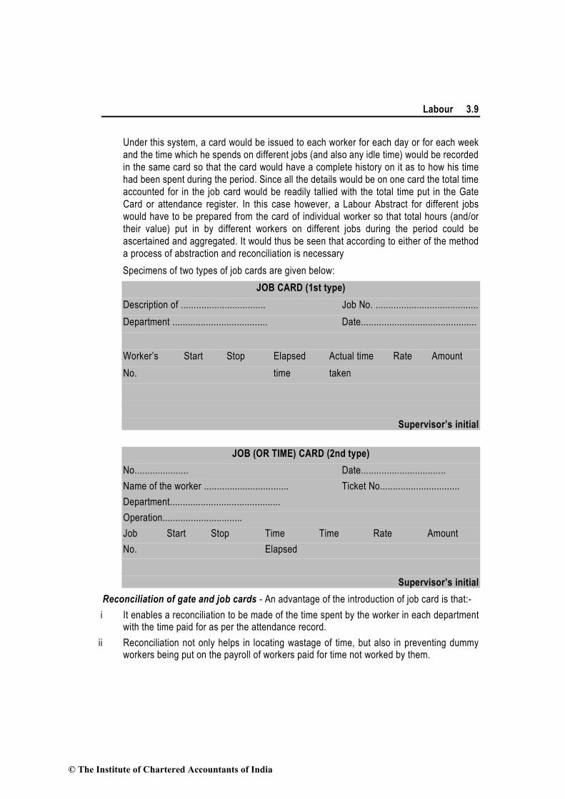
Labour 3.9
Under this system, a card would be issued to each worker for each day or for each week
and the time which he spends on different jobs (and also any idle time) would be recorded
in the same card so that the card would have a complete history on it as to how his time
had been spent during the period. Since all the details would be on one card the total time
accounted for in the job card would be readily tallied with the total time put in the Gate
Card or attendance register. In this case however, a Labour Abstract for different jobs
would have to be prepared from the card of individual worker so that total hours (and/or
their value) put in by different workers on different jobs during the period could be
ascertained and aggregated. It would thus be seen that according to either of the method
a process of abstraction and reconciliation is necessary
Specimens of two types of job cards are given below:
JOB CARD (1st type)
Description of ................................. Job No. ........................................
Department ..................................... Date.............................................
Worker’s Start Stop Elapsed Actual time Rate Amount
No. time taken
Supervisor’s initial
JOB (OR TIME) CARD (2nd type)
No..................... Date.................................
Name of the worker ................................. Ticket No...............................
Department...........................................
Operation...............................
Job Start Stop Time Time Rate Amount
No. Elapsed
Supervisor’s initial
Reconciliation of gate and job cards - An advantage of the introduction of job card is that:-
i It enables a reconciliation to be made of the time spent by the worker in each department with the time paid for as per the attendance record.
ii Reconciliation not only helps in locating wastage of time, but also in preventing dummy workers being put on the payroll of workers paid for time not worked by them.
© The Institute of Chartered Accountants of India

3.10 Cost Accounting
The two sets of records serve separate purposes.
Where payment to labour is on the time rate basis, the Gate Card is a record of the hours of work that should be paid for. Since the Gate Card merely records the hours during which the worker has been within the premises of the factory and it does not contain any details as to how those hours have been put to use by the worker in his department, a job card must be prepared to provide the necessary information. As we have already seen, the job card may be prepared either worker-wise or job-wise.
Objectives of Time-Booking - Objectives of time-booking are as follows:
1. To ensure that time paid for, according to time keeping, has been properly utilised on different jobs or work orders.
2. To ascertain the cost of each job or work order.
3. To provide a basis for the apportionment of overhead expenses over various jobs/work orders when the method for the allocation of overhead depends upon time spent on different jobs.
4. To calculate the amount of wages and bonus payable under the wage incentive system.
5. To ascertain the labour hours spent on each job and the idle labour hours.
3.4.2 Payroll procedure: Steps included in this process are as under:
Time -keeping Department
Personnel/ HR Department
Payroll Department
Cost/ Accounting Department
Employees Statutory Bodies
1. Tim
e and
Atten
dan
ce
2. Em
plo
yee Details 3. Wage and Salary sheet
4. Payment after deductions and contributions
5. Deposit of deductions and contributions
Diagram: Payroll Procedures
© The Institute of Chartered Accountants of India

Labour 3.11
1. Attendance and Time details: A detailed sheet of number of days or hours worked by
each employee (in case of time based payment) and units or percentage of work (in case
of piece rate) as reflected by the time keeping methods are sent to the payroll department
by the time keeping department. Further, payroll department with the help of time booking
records calculate any further incentives such as overtime payment, bonus to be paid to the
employees.
2. List of employees and other details: A list of employees on roll and the rate at which
they will be paid is sent by the personnel/ HR department. Payroll department should
ensure that no unauthorised person can paid.
3. Computation of wages and other incentives: Payroll department based on the details
provided by the time keeping department and personnel department calculate wages/
salary to be paid to the employees. Payroll department prepares pay slip for all employees
authorized by the personnel department and forward the same to the cost/ accounting
department for further deductions and payment.
4. Payment to the employees: Cost/ accounting department deduct all statutory deduction
such as employee’s contribution to provident fund and employee state insurance (ESI)
scheme, TDS on salary etc. After all deductions wages/ salary is paid to the employees.
5. Deposit of all statutory liabilities: All statutory deduction made from the employees
alongwith employer’s contributions such as provident fund and employee state insurance
scheme are paid to the respective statutory bodies.
6. Investigation: Should a clock card (attendance sheet) for an employee not listed on the
payroll sheet be found, investigation of its propriety is required. Likewise, there should be
an explanation for any missing clock cards deductions: After the gross earnings (that is,
the total amount earned by an employee before any deductions are taken into
consideration) have been calculated for every employee, deductions are entered on the
payroll sheet, and the net pay of each employee is determined.
The followings are generally deducted from the payroll
Type of deductions Description
Statutory Deductions
1. Provident fund Employee’s contribution to the Provident fund is deducted from the salary/ wages of the concerned employee. Employee’s contribution to the fund shall be equal to contribution payable by the employer.
2. Employee State Insurance Scheme (ESI)
Employee’s contribution to the ESI is deducted from the salary/ wages. Currently, the employee’s contribution rate (w.e.f. 1.1.97) is 1.75% of the wages
3. Tax Deduction at Source (TDS)
Employer is obliged to deduct tax at source if it will be paying to the employee net salary exceeding maximum exemption limit
© The Institute of Chartered Accountants of India

3.12 Cost Accounting
in equal installments.
4. Professional Tax In India, the professional tax is imposed at the state level. Business owners, working individuals, merchants and people carrying out various occupations comes under the purview of this tax. Professional tax is deducted based on predetermined slabs.
Other Deductions
1. Voluntary contribution to Provident fund
If any employee so desires may contribute over and above the contribution payable by the employer.
2. Contribution to any benevolent fund.
An employee may contribute to any benevolent fund voluntarily by a putting a request to the payroll department.
3. Loan deductions Installments of any loan taken by the employee.
4. Other advances and dues Other advances like festival advance and unadjusted advances taken.
3.5 Idle Time
It is a time during which no production is carried out because the worker remains idle even
though they are paid. Idle time can be normal idle or abnormal idle time.
Normal idle time: It is the time which cannot be avoided or reduced in the normal course of
business.
Causes Treatment
1. The time lost between factory gate and the place of work
2. The interval between one job and another
3. The setting up time for the machine
4. Normal fatigue etc.
It is treated as a part of the cost of production. Thus, in the case of direct workers an allowance for normal idle time is built into the labour cost rates.
In the case of indirect workers, normal idle time is spread over all the products or jobs through the process of absorption of factory overheads
Abnormal idle time: Apart from normal idle time, there may be factors which give rise to
abnormal idle time.
Causes Treatment
1. Idle time may also arise due to abnormal factors like lack of coordination
2. Power failure, Breakdown of machines
3. Non-availability of raw materials, strikes, lockouts, poor supervision, fire,
Abnormal idle time cost is not included as a part of production cost and is shown as a separate item in the Costing Profit and Loss Account.
The cost of abnormal idle time should be further categorised into controllable and
© The Institute of Chartered Accountants of India

Labour 3.13
flood etc.
4. The causes for abnormal idle time should be further analysed into controllable and uncontrollable.
i) Controllable abnormal idle time refers to that time which could have been put to productive use had the management been more alert and efficient. All such time which could have been avoided is controllable idle time.
ii) Uncontrollable abnormal idle time refers to time lost due to abnormal causes, over which management does not have any control e.g., breakdown of machines, flood etc. may be characterised as uncontrollable idle time.
uncontrollable. For each category, the break-up of cost due to various factors should be separately shown. This would help the management in fixing responsibility for controlling idle time.
Management should aim at eliminating controllable idle time and on a long-term basis reducing even the normal idle time. This would require a detailed analysis of the causes leading to such idle time.
Illustration 1: (Calculation of effective hourly cost)
‘X’ an employee of ABC Co. gets the following emoluments and benefits:
(a) Basic pay ` 1,000 p.m.
(b) Dearness allowance ` 200 p.m.
(c) Bonus 20% of salary and D.A.
(d) Other allowances ` 250 p.m.
(e) Employer’s contribution to P.F. 10% of salary and D.A.
‘X’ works for 2,400 hours per annum, out of which 400 hours are non-productive and treated as
normal idle time. You are required to find out the effective hourly cost of employee ‘X’.
Solution
Statement showing computation of effective hourly cost of employee ‘X’
(i) Earning of Employee ‘X’:
Per month Per annum
(`) (`)
Basic pay 1,000 12,000
Dearness Allowance 200 2,400
Bonus 240 2,880
Employer’s contribution to provident fund 120 1,440
© The Institute of Chartered Accountants of India

3.14 Cost Accounting
Other allowance 250 3,000
1,810 21,720
(ii) Effective working hours :
Annual working hours 2,400
Less : Normal idle time 400
Effective working hours 2,000
Effective hourly cost of ‘X’ : ` 21,720/2,000 10.86
3.6 Overtime
Overtime premium: Work done beyond normal working hours is known as ‘overtime work’.
Overtime payment is the amount of wages paid for working beyond normal working hours. The
rate for overtime work is higher than the normal time rate; usually it is at double the normal
rates. The extra amount so paid over the normal rate is called overtime premium.
As per the Factories Act 1948 “ Where a worker works in a factory for more than nine hours in any day or for more than fortyeight hours in any week, he shall, in respect of overtime work, be entitled to wages at the rate of twice his ordinary rate of wages.”
Where any workers in a factory are paid on a piece-rate basis, the time rate shall be deemed to be equivalent to the daily average of their full-time earnings for the days on which they actually worked on the same or identical job during the month immediately preceding the calendar month during which the overtime work was done, and such time rates shall be deemed to be the ordinary rates of wages of those workers
Ordinary rate of wages means the basic wages plus such allowances, including the cash equivalent of the advantage accruing through the concessional sale to workers of food grains and other articles, as the worker is for the time being entitled to, but does not include a bonus and wages for overtime work.
Occasional overtime is a healthy sign since it indicates that the firm has the optimum capacity
and that the capacity is being fully utilised. But persistent overtime is rather a bad sign because
it may indicate either (a) that the firm needs larger capacity in men and machines, or (b) that
men have got into the habit of postponing their ordinary work towards the evening so that they
can earn extra money in the form of overtime wages.
Causes of Overtime and Treatment of Overtime premium in cost accounting
Causes Treatment
(1) The customer may agree to bear the entire charge of overtime because of urgency of work.
(1) If overtime is resorted to at the desire of the customer, then overtime premium may be charged to the job directly.
(2) Overtime may be called for to make up (2) If overtime is required to cope with
© The Institute of Chartered Accountants of India
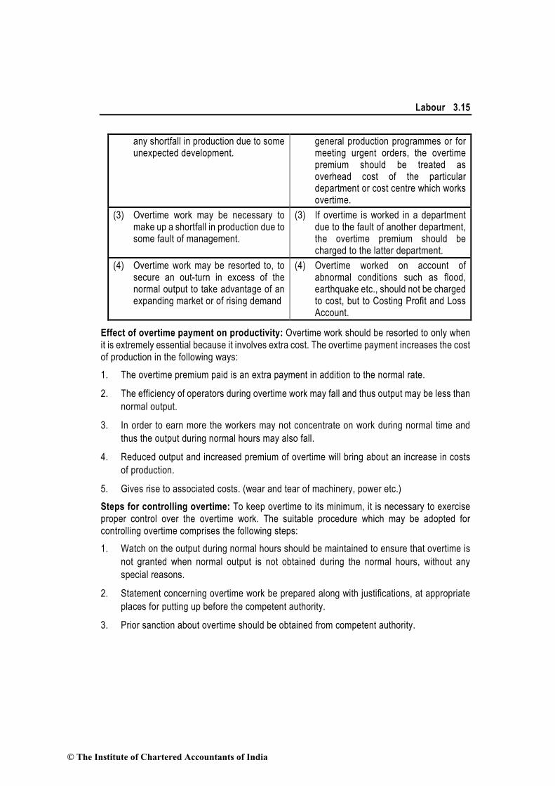
Labour 3.15
any shortfall in production due to some unexpected development.
general production programmes or for meeting urgent orders, the overtime premium should be treated as overhead cost of the particular department or cost centre which works overtime.
(3) Overtime work may be necessary to make up a shortfall in production due to some fault of management.
(3) If overtime is worked in a department due to the fault of another department, the overtime premium should be charged to the latter department.
(4) Overtime work may be resorted to, to secure an out-turn in excess of the normal output to take advantage of an expanding market or of rising demand
(4) Overtime worked on account of abnormal conditions such as flood, earthquake etc., should not be charged to cost, but to Costing Profit and Loss Account.
Effect of overtime payment on productivity: Overtime work should be resorted to only when
it is extremely essential because it involves extra cost. The overtime payment increases the cost
of production in the following ways:
1. The overtime premium paid is an extra payment in addition to the normal rate.
2. The efficiency of operators during overtime work may fall and thus output may be less than
normal output.
3. In order to earn more the workers may not concentrate on work during normal time and
thus the output during normal hours may also fall.
4. Reduced output and increased premium of overtime will bring about an increase in costs
of production.
5. Gives rise to associated costs. (wear and tear of machinery, power etc.)
Steps for controlling overtime: To keep overtime to its minimum, it is necessary to exercise
proper control over the overtime work. The suitable procedure which may be adopted for
controlling overtime comprises the following steps:
1. Watch on the output during normal hours should be maintained to ensure that overtime is
not granted when normal output is not obtained during the normal hours, without any
special reasons.
2. Statement concerning overtime work be prepared along with justifications, at appropriate
places for putting up before the competent authority.
3. Prior sanction about overtime should be obtained from competent authority.
© The Institute of Chartered Accountants of India

3.16 Cost Accounting
4. Actual rate of output produced during the overtime period should be compared with normal
rate of output.
5. Periodical reports on overtime wages should be sent to top management for taking
corrective action.
6. If possible an upper limit may be fixed for each category of workers in respect of overtime.
Illustration 2: (Calculation of earnings)
Calculate the earnings of A and B from the following particulars for a month and allocate the
labour cost to each job X, Y and Z:
A B
(i) Basic Wages (`) 100 160
(ii) Dearness Allowance 50% 50%
(iii) Contribution to provident Fund (on basic wages) 8% 8%
(iv) Contribution to Employee’s State Insurance (on basic wages) 2% 2%
(v) Overtime (Hours) 10 --
The normal working hours for the month are 200. Overtime is paid at double the total of normal
wages and dearness allowance. Employer’s contribution to state Insurance and Provident Fund
are at equal rates with employees contributions. The two workers were employed on jobs X, Y
and Z in the following proportions:
Jobs X Y Z
Worker A 40% 30% 30%
Worker B 50% 20% 30%
Overtime was done on job Y.
Answer
Statement showing Earnings of Workers A and B
A (`) B (`)
Basic wages 100.00 160.00
Dearness Allowance (50% of Basic Wages) 50.00 80.00
Overtime wages (Refer to Working Note 1) 15.00 --
Gross wages earned 165.00 240.00
Less: Contribution to Provident fund (8.00) (12.80)
Less: Contribution to ESI (2.00) (3.20)
Net wages earned 155.00 224.00
© The Institute of Chartered Accountants of India

Labour 3.17
Statement of Labour Cost
A (`) B (`)
Gross Wages (excluding overtime) 150.00 240.00
Add: Employer’s contribution to PF 8.00 12.80
Add: Employer’s contribution to ESI 2.00 3.20
Gross wages earned 160.00 256.00
Normal working hours 200 200
Ordinary wages arte per hour 0.80 1.28
Statement Showing Allocation of Wages to Jobs
Total Wages
(`)
Jobs
X (`) Y (`) Z (`)
Worker A:
- Ordinary Wages (4: 3 : 3) 160.00 64.00 48.00 48.00
- Overtime 15.00 -- 15.00 --
Worker B:
- Ordinary Wages (5 : 2 : 3) 256.00 128.00 51.20 76.80
431.00 192.00 114.20 124.80
Working Notes
1. Normal Wages are considered as basic wages
Over time = ( )2 Basic wage + DA 10 hours
200
× ×
= 150
2 10 hours200
× ×
` = 1.50 × 10 hours = ` 15
Illustration 3: (Calculation of overtime premium)
It is seen from the job card for repair of the customer’s equipment that a total of 154 labour
hours have been put in as detailed below:
Worker ‘A’ paid at ` 200 per day of 8 hours
Worker ‘B’ paid at ` 100 per day of 8 hours
Worker ‘C’ paid at ` 300 per day of 8 hours
Monday (hours) 10.5 8.0 10.5
Tuesday (hours) 8.0 8.0 8.0
© The Institute of Chartered Accountants of India

3.18 Cost Accounting
Wednesday (hours) 10.5 8.0 10.5
Thursday (hours) 9.5 8.0 9.5
Friday (hours) 10.5 8.0 10.5
Saturday (hours) -- 8.0 8.0
Total (hours) 49.0 48.0 57.0
In terms of an award in a labour conciliation, the workers are to be paid dearness allowance on
the basis of cost of living index figures relating to each month which works out @ ` 968 for the
relevant month. The dearness allowance is payable to all workers irrespective of wages rate if
they are present or are on leave with wages on all working days.
Sunday is a weekly holiday and each worker has to work for 8 hours on all week days and 4 hours
on Saturdays; the workers are however paid full wages for Saturday (8 hours for 4 hours worked).
Workers are paid overtime according to the Factories Act, 1948. Excluding holidays the total
number of hours works out to 176 in the relevant month. The company’s contribution to Provident
Fund and Employees State Insurance Premium are absorbed into overheads.
Work out the wages payable to each worker.
Solution
(1) Calculation of hours to be paid for worker A :
Normal hours
Extra hours
Overtime hours
Equivalent normal hours for overtime worked
Total normal hours
Monday 8 1 1½ 3 12
Tuesday 8 -- -- -- 8
Wednesday 8 1 1½ 3 12
Thursday 8 1 ½ 1 10
Friday 8 1 1½ 3 12
Saturday -- -- -- -- --
Total 40 4 5 10 54
Calculation of hours to be paid for worker B :
Normal hours
Extra hours
Overtime hours
Equivalent normal hours for overtime worked
Total normal hours
Monday 8 --- --- --- 8
Tuesday 8 --- --- --- 8
Wednesday 8 --- --- --- 8
© The Institute of Chartered Accountants of India

Labour 3.19
Thursday 8 --- --- --- 8
Friday 8 --- --- --- 8
Saturday 4 4* --- --- 8
Total 44 4 --- --- 48
(*Worker-B has neither worked more than 9 hours in any day nor more than 48 hours in the week)
Calculation of hours to be paid for worker C :
Normal hours
Extra hours
Overtime hours
Equivalent normal hours for overtime worked
Total normal hours
Monday 8 1 1½ 3 12
Tuesday 8 --- --- --- 8
Wednesday 8 1 1½ 3 12
Thursday 8 1 ½ 1 10
Friday 8 1 1½ 3 12
Saturday 4 --- 4* 8 12
Total 44 4 9 18 66
(*Worker-C has worked more than 48 hours in the week)
Wages payable:
A B C
Basic Wages per hour (`) 25.00 12.50 37.50
Dearness allowance per hour (`) 5.50 5.50 5.50
Hourly rate (`) 30.50 18.00 43.00
Total normal hours 54.00 48.00 66.00
Total Wages payable (`) 1,647.00 864.00 2,838.00
Illustration 4: (Calculation of labour cost chargeable to a job)
In a factory, the basic wage rate is ` 10 per hour and overtime rates are as follows :
Before and after normal working hours : 175% of basic wage rate
Sundays and holidays : 225% of basic wage rate
During the previous year, the following hours were worked :
Normal time : 1,00,000 hours
Overtime before and after working hours : 20,000 hours
© The Institute of Chartered Accountants of India

3.20 Cost Accounting
Overtime on Sundays and holidays : 5,000 hours
Total : 1,25,000 hours
The following hours have been worked on job ‘Z’ :
Normal : 1,000 hours.
Overtime before and after working hrs. : 100 hours.
Sundays and holidays : 25 hours.
Total : 1,125 hours.
You are required to calculate the labour cost chargeable to job ‘Z’ and overhead in each of the following instances:
(a) Where overtime is worked regularly throughout the year as a policy due to the labour
shortage.
(b) Where overtime is worked irregularly to meet the requirements of production.
(c) Where overtime is worked at the request of the customer to expedite the job.
Solution
Workings
Computation of average inflated wage rate (including overtime premium) :
Basic wage rate : ` 10 per hour
Overtime wage rate before and after working hours : ` 10 × 175% = ` 17.50 per hour
Overtime wage rate for Sundays and holidays : ` 10 × 225% = ` 22.50 per hour
Annual wages for the previous year for normal time : 1,00,000 hrs. × ` 10 = ` 10,00,000
Wages for overtime before and after working hours : 20,000 hrs. × ` 17.50=` 3,50,000
Wages for overtime on Sundays and holidays : 5,000 hrs. × ` 22.50 = ` 1,12,500
Total wages for 1,25,000 hrs. = `14,62,500
Average inflated wage rate : 14,62,500
1,25,000hours
`= `11.70
(a) Where overtime is worked regularly as a policy due to labour shortage, the overtime premium is treated as a part of labour cost and job is charged at an inflated wage rate.
Hence,
Labour cost chargeable to job Z = Total hours × Inflated wage rate = 1,125 hrs. × ` 11.70 = ` 13,162.50
(b) Where overtime is worked irregularly to meet the requirements of production, basic wage rate is charged to the job and overtime premium is charged to factory overheads as under :
© The Institute of Chartered Accountants of India

Labour 3.21
Labour cost chargeable to
Job Z : 1,125 hours @ ` 10 per hour = ` 11,250.00
Factory overhead : 100 hrs. × ` (17.50 – 10) = ` 750.00
25 hrs. × ` (22.50 – 10) = ` 312.50
Total factory overhead ` 1,062.50
(c) Where overtime is worked at the request of the customer, overtime premium is also
charged to the job as under :
(`)
Job Z labour cost 1,125 hrs. @ ` 10 = 11,250.00
Overtime premium 100 hrs. @ ` (17.50 – 10) = 750.00
25 hrs. @ ` (22.50 – 10) = 312.50
Total 12,312.50
3.7 Labour Turnover
Labour turnover in an organisation is the rate of change in the composition of labour
force during a specified period measured against a suitable index.
The standard of usual labour turnover in the industry or locality or the labour turnover rate for a
past period may be taken as the index or norm against which actual turnover rate is compared.
There are three methods of calculating labour turnover which are given below :
(i) Replacement method : This method takes into consideration actual replacement of labour
irrespective of number of persons leaving
=Number of employees replaced
100Average number of employees on roll
×
New labour appointed on account of expansion not to be included in number of
replacements
(ii) Separation method: In this method labour turnover is measured by dividing the total
number of separations during the period by the average total number of workers on payroll
during the same period
= Number of employees separated during the year
100Average number of employees on roll during the period
×
(iii) Flux method: This method takes into account both the number of replacements as well as
the number of separations during the period
= Number of employees separated Number of employees replaced
100Average number of employees on roll during the period
+×
© The Institute of Chartered Accountants of India

3.22 Cost Accounting
Labour turnover due to new recruitment: Workers joining a business concern on account
of its expansion do not account for labour turnover. But these newly recruited workers are
certainly responsible for a change in the composition of labour force, due to this feature,
some cost accountants measure workers to the extent of new (excluding replacements)
joining the labour force as follows :
No. of new workers joining in a period (excluding replacements)
Average number of workers on the roll in a period× 100
The total number of workers joining, including replacements, is called accessions.
The labour turnover rate, in such a case, may also be computed in respect of total number
of workers joining (accessions) the business concern, during a given period both on account
of replacements and because of expansion is as under:
No.of accessions in a period
Average number of wor ker s in a period
× 100
When number of accessions are considered for measuring labour turnover, the labour turnover
rate by flux method may be computed by using any one of the following expressions:
Labour turnover rate (Flux method) =
No. of separations No. of replacements No. of new recruitments100
Average number of wor ker s
+ +×
OR
100× workersof number Average
accessions of No. + sseparation of No.
The above rate of labour turnover indicates the total effect of number of workers separated, number of workers replaced and number of new workers recruited and joined the concern on account of its expansion, etc.
If in the above computations, the data given is for a period other than a year, the labour turnover rate so computed may be converted into equivalent annual labour turnover rate by the following formula:
Equivalent annual labour turnover rate = period the in days of Number
period the for rate Turnover× 365
Causes of Labour Turnover : The main causes of labour turnover in an organization/ industry
can be broadly classified under the following three heads :
(a) Personal Causes;
(b) Unavoidable Causes; and
© The Institute of Chartered Accountants of India

Labour 3.23
(c) Avoidable Causes.
Personal causes are those which induce or compel workers to leave their jobs; such causes
include the following:
(i) Change of jobs for betterment.
(ii) Premature retirement due to ill health or old age.
(iii) Domestic problems and family responsibilities.
(iv) Discontent over the jobs and working environment.
In all the above cases the employee leaves the organisation at his will and, therefore, it is difficult
to suggest any possible remedy in the first three cases.
But the last one can be overcome by creating conditions leading to a healthy working
environment. For this, officers should play a positive role and make sure that their subordinates
work under healthy working conditions.
Unavoidable causes are those under which it becomes obligatory on the part of management to
ask one or more of their employees to leave the organisation; such causes are summed up as
listed below:
(i) Seasonal nature of the business;
(ii) Shortage of raw material, power, slack market for the product etc.;
(iii) Change in the plant location;
(iv) Disability, making a worker unfit for work;
(v) Disciplinary measures;
(vi) Marriage (generally in the case of women).
Avoidable causes are those which require the attention of management on a continuous basis
so as to keep the labour turnover ratio as low as possible. The main causes under this case are
indicated below :
(1) Dissatisfaction with job, remuneration, hours of work, working conditions, etc.,
(2) Strained relationship with management, supervisors or fellow workers;
(3) Lack of training facilities and promotional avenues;
(4) Lack of recreational and medical facilities;
(5) Low wages and allowances.
Proper and timely management action can reduce the labour turnover appreciably so far as
avoidable causes are concerned.
Effects of Labour Turnover: High labour turnover increases the cost of production in the
following ways:
© The Institute of Chartered Accountants of India

3.24 Cost Accounting
(i) Even flow of production is disturbed;
(ii) Efficiency of new workers is low; productivity of new but experienced workers is low in the
beginning;
(iii) There is increased cost of training and induction;
(iv) New workers cause increased breakage of tools, wastage of materials, etc.
In some companies, the labour turnover rates are as high as 100%; it means that on the
average, all the work is being done by new and inexperienced workers. This is bound to
reduce efficiency and production and increases the cost of production.
(v) Cost of recruitment and training increases.
Two types of costs which are associated with labour turnover are :
(a) Preventive costs: These include costs incurred to keep the labour turnover at a low
level, i.e. cost of medical services, welfare schemes and pension schemes. If a company incurs
high preventive costs, the rate of labour turnover is usually low.
(b) Replacement costs: These are the costs which arise due to high labour turnover. If men
leave soon after they acquire the necessary training and experience of good work, additional
costs will have to be incurred on new workers, i.e., cost of employment, training and induction,
abnormal breakage and scrap and extra wages and overheads due to the inefficiency of new
workers.
It is obvious that a company will incur very high replacement costs if the rate of labour turnover
is high. Similarly, only adequate preventive costs can keep labour turnover at a low level. Each
company must, therefore, work out the optimum level of labour turnover keeping in view its
personnel policies and the behaviour of replacement cost and preventive costs at various levels
of labour turnover rates.
Remedial Steps To Minimise Labour Turnover - The following steps are useful for minimising
labour turnover.
1. Exit interview: An interview be arranged with each outgoing employee to ascertain the
reasons of his leaving the organisation.
2. Job analysis and evaluation: Before recruiting workers, job analysis and evaluation may
be carried out to ascertain the requirements of each job.
3. Scientific system of recruitment, placement and promotion: The organisation should
make use of a scientific system of recruitment, selection, placement and promotion for
employees.
4. Enlightened attitude of management: The management should introduce the following
steps for creating a healthy working atmosphere:
(i) Service rules should be framed, discussed and approved among management and
workers, before their implementation.
© The Institute of Chartered Accountants of India

Labour 3.25
(ii) Provide facilities for education and training of workers.
(iii) Introduce a procedure for settling worker’s grievances.
5. Use of committee: Issues like control over workers, handling their grievances etc., may
be dealt by a committee, comprising of members from management and workers.
Illustration 5: (Calculation of cost of labour turnover)
The management of Bina and Rina Ltd. are worried about their increasing labour turnover in the
factory and before analyzing the causes and taking remedial steps, they want to have an idea
of the profit foregone as a result of labour turnover in the last year.
Last year sales amounted to ` 83,03,300 and P/V ratio was 20 per cent. The total number of actual hours worked by the Direct Labour force was 4.45 lakhs. As a result of the delays by the Personnel Department in filling vacancies due to labour turnover, 1,00,000 potentially productive hours were lost. The actual direct labour hours included 30,000 hours attributable to training new recruits, out of which half of the hours were unproductive.
The costs incurred consequent on labour turnover revealed, on analysis, the following:
Settlement cost due to leaving ` 43,820
Recruitment costs ` 26,740
Selection costs ` 12,750
Training costs ` 30,490
Assuming that the potential production lost as a consequence of labour turnover could have been sold at prevailing prices, find the profit foregone last year on account of labour turnover.
Solution
Determination of contribution foregone
Actual hours worked (given) 4,45,000
Less : Unproductive training hours 15,000
Actual productive hours 4,30,000
The potentially productive hours lost are 1,00,000
Sales lost for 1,00,000 hours = 83,03,300
4,30,000 hrs
`
× 1,00,000 hrs = ` 19,31,000
Contribution lost for 1,00,000 hrs.
=19,31,000
100
`× 20 = ` 3,86,200
© The Institute of Chartered Accountants of India

3.26 Cost Accounting
Statement showing profit foregone last year on account of labour turnover of Bina and Rina Ltd.
(`)
Contribution foregone ( as calculated above) 3,86,200
Settlement cost due to leaving 43,820
Recruitment cost 26,740
Selection cost 12,750
Training costs 30,490
Profit foregone 5,00,000
Illustration 6: (Calculation of workers recruited, joined and discharged)
The Cost Accountant of Y Ltd. has computed labour turnover rates for the quarter ended 31st March, 20X1 as 10%, 5% and 3% respectively under ‘Flux method’, ‘Replacement method’ and ‘Separation method’ respectively. If the number of workers replaced during that quarter is 30, find out the number of:
(1) workers recruited and joined and (2) workers left and discharged.
Solution
Working Note:
Average number of workers on roll:
100×roll on workersof number Average
tsreplacemen of No. = methodt replacemen under rate turnover Labour
Or, 100
5 =
roll on workersof number Average
30
Or Average number of workers on roll = 5
10030×= 600
(1) Number of workers recruited and joined :
Labour turnover rate (Flux method) = roll on workersof number Average
(A)accessions of No.(S)*sseparation of No. +× 100
Or 100
10 =
600
A*18 +
Or A =
−18
100
6000 = 42
No. of workers recruited and joined 42.
(2) Number of workers left and discharged :
Labour turnover rate (Separation method) = roll on workersof number Average
s(S)separation of No. × 100
© The Institute of Chartered Accountants of India

Labour 3.27
100
3=
600
S
Or S* = 18
Hence, number of workers left and discharged comes to 18.
3.8 Incentive System
3.8.1 Important factors necessary for introducing of an incentive system: An
incentive can be defined as the stimulation for effort and effectiveness by offering monetary
inducement or enhanced facilities. It may be provided individually or collectively.
It may be monetary in the form of a bonus where the employee gets a reward for his efforts directly
or non-monetary tending to improve living and working conditions where a group of employees or
individuals share the reward arising out of their combined effort in equitable production.
The main factors that should be taken into account before introducing a scheme of incentives
are stated below:
(i) System of Quality Control: The need for producing goods of high quality or those having
very good workmanship or finish and the manner this can be ensured. Only if a system of
quality control can be relied upon to maintain the quality of goods of the standard required,
an incentive scheme should be introduced; otherwise, workers should be paid on time
basis.
(ii) Maximise production: The need to maximise production—thus required incentives to be
given to workers. But sometimes workmanship is more important than quantity of output;
in such cases, incentive schemes of wage payment are not suitable.
(iii) Precision in measuring quantity of Work: Where the quantity of work done cannot be
measured precisely, incentive schemes cannot be offered.
(iv) Role of Management in Incentive Schemes: The role of management and workers in
achieving greater efficiency, if it is unnecessary for the management to constantly plan
work, for example, when the work is repetitive, workers should be offered good incentives
to achieve high efficiency; but in case management is constantly required to plan the work,
as in the case of job work, the management should share the fruits of extra efficiency
achieved. This factor determines the choice of a particular incentive scheme.
(v) Effort of Workers: Whether the quantity of output is within the control of the worker and if
so, to what extent. Sometimes, as in the case of chain assembly work the output is not
dependent on the effort put in by workers; incentive schemes in such cases are not suit-
able.
(vi) Standards of Performance: The exactitude with which standards of performance can be
laid down. Fixation of standard is necessary for the introduction of a scheme of incentives.
When this requires heavy expenditure, incentive schemes may be rather costly.
© The Institute of Chartered Accountants of India

3.28 Cost Accounting
(vii) No Discrimination: The effect of an incentive scheme for one set of workers on other
workers. If for instance, an incentive scheme makes it possible for unskilled workers to
earn high wages, the wage rates for skilled workers must also be raised (if they are paid
on time basis) to avoid dissatisfaction among them. In that event, the incentive scheme
may raise labour cost instead of lowering it.
(viii) Comparative Study: The system of wage payment prevailing in other areas and industries
or similar occupations. If possible, there should be uniformity.
(ix) Attitude of Workers: The attitude of labour and trade unions towards incentive schemes.
Workers usually like to have a certain guaranteed time-basis wage but also like to earn
extra through an incentive scheme.
On the whole, the system of wage payment should be such as would increase production without
lowering quality. This will increase the surplus and will enable the employer to pay higher wages
which, in turn, will lead to higher output.
3.8.2 Main principles for a sound system of wage incentive: The objective of wage
incentives is to improve productivity and increase production so as to bring down the unit cost
of production.
In order to make the incentive scheme effective and useful, the following general principles have to be considered while designing a sound system of wage incentives.
(i) Just and Fair: The reward for a job should be linked with the effort involved in that job and
the scheme should be just and fair to both employees and employers. This involves the
following:
(a) The standard required of the workers should be carefully set, if possible through
proper time and motion studies.
(b) If the work is of repetitive type, the entire benefit of the time saved should be available
to the worker but, in the case of non-standardised work or where precise standards
cannot be set, the benefit of the time saved, if any, should be shared by the employer,
the supervisor and the worker.
(ii) Well defined scheme: The scheme should be clearly defined and be capable of being
understood by the employees easily. The standards set should be such that they can be
achieved even by average employees. While standards are being set, the workers
concerned should be consulted.
(iii) Worker’s Expectations: As far as possible, no limit should be placed on the amount of additional earnings; otherwise it will dampen the initiative of the workers. In this regard, what is important is not what actually prevails but what the workers think—if they think, even wrongly, that the employer will stop wages from rising beyond a certain limit, the incentive scheme may not be really effective.
© The Institute of Chartered Accountants of India

Labour 3.29
(iv) Stability: The scheme should be reasonable and stable, and should not be changed or modified too often without consulting the employees.
(v) Charge on employees: The scheme should take care that the employees are not penalised for reasons beyond their control.
(vi) Incentive based on quality: The scheme should provide for inspection of output so that only good pieces qualify for incentives. It would even be better not to introduce any incentive scheme if workmanship is of vital importance in sales.
(vii) Adequate Resources: The management should ensure that there is no cause for complaint by the workers that they are sitting idle, say for want of tools or materials. Management has to see that there is, as far as practicable, no interruption of production.
(viii) Limited Costs: The operation of the scheme should not entail heavy clerical costs. In fact the scheme should facilitate the introduction of budgetary control and standard costing.
(ix) Morale booster: It should be capable of improving the morale of the employees and it should be in conformity with the local trade union agreements and other government regulations.
(x) Guaranteed wages: There should be a guaranteed wage on time basis which generally works as a good psychological boost to incentive scheme.
(xi) Equality in payment: the effect of incentive scheme on those who cannot be covered should be gauged and taken note of. Sometimes, highly skilled workers have perforce to be paid on time basis whereas semiskilled or unskilled workers may be put on incentive scheme. If the latter earn more than former, the incentive schemes on the whole prove harmful.
Essential characteristics of a good incentive system: to recapitulate
(i) It should be just both to the employer and to the employee. It should be positive and not
unnecessarily punitive and so operated as to promote confidence.
(ii) It should be strong both ways i.e. it should have a standard task and a generous return.
The latter should be in direct proportion to employee’s efforts. It should reflect the
employer’s contribution to the success of the company.
(iii) It should be unrestricted as to the amount of the earning.
(iv) It should be reasonable, apart from being simple, for employee to figure out his incentive
in relation to his individual performance, as far as practicable.
(v) It should be flexible and intimately related to other management controls.
(vi) It should automatically assist supervision and, when necessary, aid team work.
(vii) It should have employee’s support and in no way should it be paternalistic.
(viii) It should have managerial support in so far as production material, quality control,
maintenance and non-financial incentives are concerned.
© The Institute of Chartered Accountants of India

3.30 Cost Accounting
(ix) It should not be used temporarily and dropped in recession times as means of wage
reduction.
(x) There should be correct measurement of the effort made for incentive purpose.
Measurement of effort is made by time and motion study and based on job evaluation; the
rates of wages are fixed for different operations.
3.9 Labour Utilisation
For identifying utilisation of labour a statement is prepared (generally weekly) for each
department / cost centre. This statement should show the actual time paid for, the standard time
(including normal idle time) allowed for production and the abnormal idle time analysed for
causes thereof.
3.9.1 Identification of utilisation of labour with cost centres : For the identification of
utilisation of labour with the cost centre a wage analysis sheet is prepared.
Wage analysis sheet is a columnar statement in which total wages paid are analysed according
to cost centre, jobs, work orders etc. The data for analysis is provided by wage sheet, time card,
piece work cards and job cards.
The preparation of such sheet serves the following purposes:
(i) It analyse the labour time into direct and indirect labour by cost centres, jobs, work orders.
(ii) It provides details of direct labour cost comprises of wages, overtime to be charged as
production cost of cost centre, jobs or work orders.
(iii) It provides information for treatment of indirect labour cost as overhead expenses.
Wage Analysis Sheet
No. week- Department/ Total Work in Factory Administration Selling &
ending cost centre progress Overhead Overhead control Distribution
control A/c A/c overhead
control A/c
3.9.2 Identification of labour hours with work order or batches or capital job: For
identification of labour hours with work order or batches or capital jobs or overhead work orders
the following points are to be noted :
(i) The direct labour hours can be identified with the particular work order or batches or capital
job or overhead work orders on the basis of details recorded on source document such as
time sheet or job cards.
(ii) The indirect labour hours cannot be directly identified with the particular work order or
batches or capital jobs or overhead work orders. Therefore, they are traced to cost centre
© The Institute of Chartered Accountants of India

Labour 3.31
and then assigned to work order or batches or capital jobs or overhead work orders by
using overhead absorption rate.
3.10 Systems of Wage Payment and Incentives
There exist several systems of employee wage payment and incentives, which can be classified
under the following heads:
The formulas for different wage payment and incentive systems are given below:
1 Time Rate System
Earnings = Hours worked × Rate per hour
2 Straight Piece Rate System
Earnings = Number of units × Piece rate per unit
3 Differential piece Rate System
3.1 F.W. Taylor’s System
Efficiency Payment
Less than 100% 83% of the normal piece rate or 80% of piece rate
when below standard
Piece
Work
Combination of time and Piece Work
Premium Bonus Methods
Group system of wage
payment
System Incentive Schemes for Indirect Workers
Straight Piece
Work
Differential Piece Work
Tylor
System
Merrick System
Halsey and Halsey Weir
Systems
Rowan
System
Barth
System
Gantt Task and Bonus System
Emerson’s efficiency System
Points
Scheme
Accelerated Premium system
Beadaux
Syst. Haynes
Syst.
SYSTEMS OF WAGE PAYMENT & INCENTIVES
Time Rate Systems Payment by Results
Time Rate
System
High Wage
Plan
Measured Day Work
Differential Time Rate
© The Institute of Chartered Accountants of India

3.32 Cost Accounting
Either 100% or 125% of the normal piece rate or 120% of piece
rate more than 100% when at or above standard
3.2 Merrick Differential Piece Rate System
Efficiency Payment
Up to 83 % Ordinary piece rate
83% to 100% 110% of ordinary piece rate (10% above the
ordinary piece rate)
Above 100% 120% or 130% of ordinary piece rate (20% to 30%
of ordinary piece rate)
4 Combination of Time and Piece Rate
4.1 Gantt Task and Bonus System
Output Payment
Output below standard Guaranteed time rate
Output at standard 120% of time rate
Output above standard 120% of piece rate
4.2 Emerson Efficiency System
Earning is calculated as follows :
Efficiency Payment
Below 66-2/3% No bonus, only guaranteed time rate is paid.
66-2/3% to 100% Worker is paid by hourly rate for the time he actually
worked plus an increase in bonus according to degree of
efficiency on the basis of step bonus rates. Bonus rate
can be up to 20%.
Above 100% 120% of time wage rate plus additional bonus of 1% for
each 1% increase in efficiency.
4.3 Bedaux Point System
Earnings = Hours worked × Rate per hour +
75 Bedaux pointssaved
Rate per hour100 60
× ×
4.4 Haynes Manit Systems
This system is similar to Bedaux Point system. Instead of Bedaux points
saved, ‘MANIT’ (Man-minutes) saved are measured for payment of bonus.
Bonus is distributed as follows :
50% bonus to the workers
10% bonus to the supervisors
40% bonus to the employer
© The Institute of Chartered Accountants of India

Labour 3.33
4.5 Accelerated Premium System
In this system individual employer makes his own formula. The following
formula may be used for a general idea of the scheme:
Y= 0.8 × x2
Where
y= wages
x= efficiency
5 Premium Bonus Plan
5.1 Halsey Premium Plan
Earnings = Hours worked × Rate per hour +
×× hour) per Ratesaved Time
100
50
5.2 Halsey-Weir Premium Plan
Earnings = Hours worked × Rate per hour +
×× hour) per Ratesaved Time
100
30
5.3 Rowan System
Earnings = Hours worked × Rate per hour +
×× hour) per Rate workedHours
allowed Time
saved Time
5.4 Barth Sharing Plan
Earnings = Rate per hour × workedHourshours Standard × 5.5 Scanlon Plan
Bonus Percentage = Revenue Sales AnnualAverage
Wages and Salaries AnnualAverage
One should remember that Provident Fund, Employees State Insurance Scheme Premium and
bonus are payable on the basic wages, dearness allowance and value of food concession.
3.10.1 Time Rate System
Meaning Suitability
Under this system, the worker is paid by the hour, day, week, or month. The amount of wages due to a worker are arrived at by multiplying the time worked (as shown by the gate card) by the appropriate time rate.
(1) Persons whose services cannot be directly or tangibly measured, e.g., general helpers, supervisory and clerical staff etc.
(2) Workers engaged on highly skilled
© The Institute of Chartered Accountants of India

3.34 Cost Accounting
jobs or rendering skilled services, e.g., tool making, inspection and testing.
(3) Where the pace of output is independent of the operator, e.g., automatic chemical plants.
Merits Demerits
(i) Simple to understand and to calculate wages.
(ii) Reduces temptation on the part of workers to increase the output at the cost of quality.
(iii) Unity in labour, no distinction between efficient and inefficient labour due to quality of production.
(iv) Stability in wages
(i) No monetary incentive to raise the level of production.
(ii) No distinction between the slow and the efficient worker.
(iii) The tendency is for the fall in output; this raises the cost per unit (because both labour and fixed expenses will be spread over a smaller number of units).
(iv) A firm cannot be sure of labour costs per unit under this method and, hence, may suffer a loss on quotations if already submitted.
3.10.1.1 High wage plan: This plan was first introduced by Ford Motor Company (in USA) in
order to induce workers to exercise extra effort in their work.
Under this plan a worker is paid a wage rate which is substantially higher than the rate prevailing
in the area or in the industry. In return, he is expected to maintain a very high level of
performance, both quantitative and qualitative. As a result, high rate men are not as costly or
expensive as they might appear at first sight.
High wage plan is suitable where high quality of work and also increased productivity are
required.
The advantage which may accrue from the implementation of this plan are :
(1) It is simple and inexpensive to operate.
(2) It helps in attracting highly skilled and efficient workers by providing suitable incentive.
(3) It reduces the extent of supervision.
(4) Increased productivity may result in reduction of unit labour cost.
3.10.1.2 Measured day work: According to this method the hourly rate of the time worker
consists of two parts viz, fixed and variable. The fixed element is based on the nature of the job
i.e. the rate for this part is fixed on the basis of job requirements. The variable portion varies for
© The Institute of Chartered Accountants of India

Labour 3.35
each worker depending upon his merit rating and the cost of living index. The aggregate of fixed
and variable part for a day is termed as Measured day’s work rate of a worker.
As the rate is based on two different elements, there are separate time rates not only for each
worker but also for each job. This method does not find much favour with workers due to the
following:
1. The rates fixed are not easily understood by the workers.
2. Merit rating tends to be arbitrary and unless changed at rapid intervals, the ratings will not
reflect the correct ranking of the qualities of a worker.
3.10.1.3 Differential time rate: According to this method, different hourly rates are fixed for
different levels of efficiency. Up to a certain level of efficiency the normal time or day rate is
paid. Based on efficiency level the hourly rate increases gradually. The following table shows
different differential rates :
Up to, say 75% efficiency Normal (say ` N per hr.)
From 76% to 80% efficiency 1.10 × N
From 81% to 90% efficiency 1.20 × N
From 91% to 100% efficiency 1.30 × N
From 101% to 120% efficiency 1.40 × N
As this method is linked with the output and efficiency of workers, therefore, it cannot be strictly
called as a time rate method of wage payment. This method in fact is similar to differential piece
work system.
3.10.2 Payment by result: Under this system the payment made has a direct relationship with
the output given by a worker. The attendance of the worker or the time taken by him for doing a
job has no bearing on the payment. The system of payment by results may be classified into the
following four categories:
(a) Systems in which the payment of wages is directly proportionate to the output given by workers.
(b) Systems in which the proportion of the wage payment to the worker increases progressively with increase in production.
(c) Systems in which payment rate decreases with the increase in output.
(d) Systems with earnings varying in proportions which differ at different levels of production.
3.10.2.1 Straight piece work system
Under this system of wage payment, each operation, job or unit of production is termed a piece.
A rate of payment, known as the piece rate or piece work rate is fixed for each piece. The wages
of the worker depend upon his output and rate of each unit of output; it is in fact independent of
the time taken by him. The wages paid to a worker are calculated as :
Wages = Number of units produced × Piece rate per unit.
© The Institute of Chartered Accountants of India

3.36 Cost Accounting
Considerable care and judgment are called for fixing the piece rate. If the rate fixed is too high
or too low, it would operate to the disadvantage of either the employer or the employee. Any
attempt on the part of the management to revise a piece rate, erroneously set too high, is likely
to lead to friction and conflict with labour. If on the other hand, it is too low, it would fail in its
objective. The only way all this may be avoided is by employing scientific methods of job
evaluation and time and motion study for the purpose of setting the rates.
Advantages Disadvantages
1. The system is simple to operate and also easy to understand.
1. The quality of output usually suffers.
2. The incentive provided is quite effective as the workers get the full benefit of any increase in production and the employer also gains by saving on overhead costs.
2. Maintenance of detailed statistics as regards production of individual workers is necessary.
3. Labour cost per unit being constant, these can be calculated in advance and quotations can be confidently submitted.
3. Maintenance of satisfactory discipline in the matter of arrival and departure of workers becomes somewhat difficult.
4. In the anxiety to produce as large a quantity as possible, workers may damage the machines and may also increase wast-age of materials.
5. Skilled workers and supervisors (who are often paid on time basis) may resent higher wages to unskilled workers paid on the piece basis.
3.10.2.2 Differential piece work system: This system provide for higher rewards to more
efficient workers. The main feature of all differential piece-work systems is that several piece
rates on a slab scale are fixed for a job or operation which is put on piece-work. For different
levels of output below and above the standard, different piece rates are applicable. Taylor Dif-
ferential Piece Work System and Merrick Differential Piece Rate System are two important
differential piece work systems discussed briefly as below:
(a) Taylor’s differential piece work system - The Taylor’s Differential Piece Rate System
aims at rewarding efficient workers by providing increased piece rate beyond certain level of
output.
Under this system two widely differing piece-rates are prescribed for each job. The lower rate is
83% of the normal piece rate and the higher rate is 125% of the normal piece rate. In other
words the higher rate is 150% of the lower rate. The lower rate is given to a worker when his
efficiency level is less than 100%. The higher rate is offered at efficiency level of either 100%
© The Institute of Chartered Accountants of India

Labour 3.37
or more. Due to the existence of the two piece rates, the system is known as differential piece
rate system.
Note: Some authors also use 80% and 120% of the piece rates as lower and higher rates
respectively at the efficiency levels, as indicated in the above paragraph.
Advantages Disadvantages
1. It is simple to understand and operate.
2. The incentive is very good and attractive for efficient workers.
3. It has a beneficial effect where overheads are high as increased production has the effect of reducing their incidence per unit of production.
This system is quite harsh to workers, as a slight reduction in output may result in a large reduction in the wages earned by them. This system is no longer in use in its original form, though the main idea behind it is used in many wage schemes.
Illustration 7: (Calculation of earnings under Taylor’s differential piece rate system)
Using Taylor’s differential piece rate system, find the earnings of the Amar, Akbar and Ali from
the following particulars:
Standard time per piece : 20 minutes
Normal rate per hour (in an 8 hours day) : ` 9.00
Amar produced : 23 units
Akbar produced : 24 units
Ali produced : 30 units
Solution
Earnings under Differential piece rate system
Workers Amar Akbar Ali
Standard output per day (units) 24 24 24
(8 hours x 60 minutes)/ 20 minutes
Actual output per day (units) 23 24 30
Efficiency (%) 95.83% 100% 125%
Actual output
×100Standarad output
23 unit
10024 unit
×
24 unit
10024 unit
×
30 unit
10024 unit
×
* Earning rate per unit 83% of 125% of 125% of
the piece the piece the piece
rate rate rate
Earning rate per unit (`) 2.49 3.75 3.75
(Refer to working note) (83% of `3) (125% of `3) (125% of `3)
© The Institute of Chartered Accountants of India

3.38 Cost Accounting
Earnings (`) 57.27 90.00 112.50
(23 units × ` 2.49) ( 24 units × ` 3.75) (30 units × ` 3.75)
* Under Taylor’s Differential price rate system, two widely differing price rates are prescribed for
each job. The lower rate is 83% of the normal piece rate and is applicable if efficiency of the
worker is below 100%. The higher piece rate is 125% of the normal piece rate and is applicable
if work completed is at efficiency level of 100% and above.
Working Note:
Normal rate per hour = ` 9.00
Normal rate per unit = `
9.00
S tandard production per hour=
`
9.00
3 units = ` 3
(b) Merrick Differential Piece Rate System - Under this system three piece rates for a job
are fixed. None of the fixed rates is below the normal. These three piece rates are as below:
Efficiency Piece rate applicable
Upto 83% Normal rate,
Above 83% and upto 100% 10% above normal rate.
Above 100% 20% or 30% above normal rate.
This system is an improvement over Taylor’s Differential Piece Rate System.
Illustration 8 (Calculation of earnings under Merrick differential piece rate system)
Refer to the statement of previous Illustration and compute the earnings of workers under
Merrick Differential Piece Rate System
Solution
Workers Amar Akbar Ali
* Earning rate per unit 10% above 10% above 20% above
(Refer to previous illustration) the normal the normal the normal
rate rate rate
or
30% above
the normal
Earning rate per unit (`) 3.30 3.30 3.60 or 3.90
Earnings (`) 75.90 79.20 108 or 117
(23 units × ` 3.30) (24 units × ` 3.30) (30 units × ` 3.60)
or
(30 units × ` 3.90)
Illustration 9: (Calculation of earnings under Taylor’s differential piece rate system)
Using Taylor’s differential piece rate system, find the earning of A from the following particulars:
© The Institute of Chartered Accountants of India

Labour 3.39
Standard time per piece 12 minutes
Normal rate per hour (in a 8 hours day) `20
A produced 37 units
Solution:
Actual output = 37 units
Standard output = pieceper minutes12
minutes60hrs.8 × = 40 units
Efficiency = units40
units37×100 = 92.5%
Under Taylor’s differential piece rate system, a worker is paid lower piece rate of 83%, since
his efficiency is less than 100%.
Standard production per hour = 60 minutes/12 minutes = 5 units
Normal Rate per hour = `20
Normal piece rate per unit = `20/5 units = `4
Lower piece rate per unit = `4 × 83/100 = `3.32
Total earnings = 37 units × `3.32 = `122.84
Illustration 10: (Calculation of earnings under Merrick differential piece rate system)
Calculate the earnings of workers A, B and C under Straight Piece Rate System and Merrick’s
Piece Rate System from the following particulars:
Normal Rate per Hour ` 5.40
Standard Time per Unit 1 Minute
Output per day is as follows:
Worker A – 390 Units
Worker B – 450 Units
Worker C – 600 Units
Working hours per day are 8.
Solution
Earnings of Workers under Straight Piece Rate System:
Worker A = 390 units × ` 0.09 = ` 35.10
Worker B = 450 units × ` 0.09 = ` 40.50
Worker C = 600 units × ` 0.09 = ` 54.00
© The Institute of Chartered Accountants of India

3.40 Cost Accounting
Earnings of Workers under Merrick’s Multiple Piece Rate System
Particulars A B C
Efficiency level
(Refer to working note ii)
Applicable wage rate per unit
Earnings (`)
81.25%
0.09
35.10
(390 units × 0.09)
93.75%
0.099
44.55
(450 units × 0.099)
125%
0.108*
64.80
(600 units × 0.108)
Note : *Some author suggests an increase of 30% over normal piece rate at an efficiency level of 120% or more. In such a case the rate per unit would be ` 0.117 and total earnings would come to `70.20.
Working Notes :
(i) Normal wage rate per unit = Normal Rate per Hour/Standard output per hour = ` 5.40/60 = 9 Paise
(ii) Efficiency level
Workers A B C
Actual output per day (units) 390 450 600
Standard output per day (units) 480 480 480
Efficiency level achieved
= unitsoutputStandard
unitsoutputActual×100
480
390 ×100 480
450 × 100 480
600 ×100
= 81.25% = 93.75% = 125%
3.10.3 Gantt Task and Bonus system: This system is a combination of time and piece work
system. According to this system a high standard or task is set and payment is made at time rate to a worker for production below the set standard.
If the standards are achieved or exceeded, the payment to the concerned worker is made at a
higher piece rate. The piece rate fixed under this system also includes an element of bonus the
extent of 20%. The figure of bonus to such workers is calculated over the time rate of the
workers.
Thus in its essence, the system consists of paying a worker on time basis if he does not attain
the standard and on piece basis if he does. Wages payable to workers under this plan are
calculated as under:
Output Payment
(i) Output below standard Guaranteed time rate.
(ii) Output at standard Time rate plus bonus of 20% (usually) of time rate.
(iii) Output above standard High piece rate on worker’s whole output.
© The Institute of Chartered Accountants of India

Labour 3.41
It is so fixed, so as to include a bonus of 20% of the piece rate.
Advantages Disadvantages
1. It provides good incentive for efficient
workers and at the same time protects
the less efficient by guaranteeing the
time rate.
2. It is simple to understand and operate.
3. It encourages better supervision and
planning.
The guaranteed time rate may have the
effect of weakening the urge of slower
worker to increase his output.
Illustration 11: (Calculation of wages under the Gantt system)
In a factory the standard time allowed for completing a given task (50 units), is 8 hours. The
guaranteed time wages are ` 20 per hour. If a task is completed in less than the standard time,
the high rate of 4 per unit is payable. Calculate the wages of a worker, under the Gantt system,
if he completes the task in
(i) 10 hours; (ii) 8 hours, and (iii) in 6 hours. Also ascertain the comparative rate of earnings per
hour under the three situations.
Solution
(i) When the worker performs the task in 10 hours, his earnings will be at the time wage rate
i.e. 10 hours × ` 20 per hour = ` 200.
(ii) When the worker performs the task is standard time i.e. in 8 hours, his earning will be:
8 hours × ` 20 = ` 160
Bonus @ 20% of time wages = ` 32
Total earnings ` 192
(iii) When the worker performs the task in less than the standard time his earning will be at
piece rate i.e.
50 units × ` 4 per unit = ` 200
The comparative rate of earnings per hour under the above three situations is:
(i) ` 200/10 hrs. = ` 20 per hour
(ii) ` 192/8 hrs. = ` 24 per hour
(iii) ` 200/6 hrs. = ` 33.33 per hour
3.10.4 Emerson’s Efficiency System: Under this system minimum time wages are
guaranteed. But beyond a certain efficiency level, bonus in addition to minimum day wages is given.
A worker who is able to attain efficiency, measured by his output equal to 2/3rd of the standard
efficiency, or above, is deemed to be an efficient worker deserving encouragement. The scheme
© The Institute of Chartered Accountants of India

3.42 Cost Accounting
thus provides for payment of bonus at a rising scale at various levels of efficiency, ranging from
66.67% to 150%.
The levels are as mentioned below:
(i) For a performance below 66.67% only time rate wages without any bonus are paid.
(ii) 66⅔% to 100% efficiency, bonus varies between 0.01% and 20%.
(iii) Above 100% efficiency bonus of 20% of basic wages plus 1% for each 1% increase in
efficiency is admissible.
This system is superior to one to the differential piece rate in so far as it encourages the slow
worker to do a little better than before. Also it does not pre-suppose a high degree of average
performance. Wages on time basis are guaranteed.
Illustration 12: (Earnings under Emerson Efficiency System)
From the following information you are required to calculate the bonus and earnings under
Emerson Efficiency System. The relevant information is as under:
Standard working hours : 8 hours a day
Standard output per hour in units : 5
Daily wage rate : ` 50
Actual output in units
Worker A 25 units
Worker B 40 units
Worker C 45 units
Solution
Statement showing bonus and earnings under Emerson Efficiency System
Workers A B C
Actual output in units 25 40 45
Standard output in units 40 40 40
Efficiency level (%) 62.5% 100% 112.50%
×100
output Standarad
output Actual
Rate of bonus No bonus 20% 32.50%
(20% + 12.5%)
Time wages (`) 50 50 50
Bonus (`) Nil 10 16.25
(20% of ` 50) (32.5% of ` 50)
© The Institute of Chartered Accountants of India

Labour 3.43
Total earnings (`) 50 60 66.25
3.10.5 Points Scheme or Bedeaux System: Under this scheme, firstly the quantum of work
that a worker can perform is expressed in Bedeaux points or B’s. These points represent the
standard time in terms of minutes required to perform the job. The standard numbers of points
in terms of minutes are ascertained after a careful and detailed analysis of each operation or
job. Each such minute consists of the time required to complete a fraction of the operation or
the job, and also an allowance for rest due to fatigue.
Workers who are not able to complete tasks allotted to them within the standard time are paid
at the normal daily rate.
Those who are able to improve upon the efficiency rate are paid a bonus, equal to the wages
for time saved as indicated by excess of B’s earned (standard minutes for work done) over
actual time. Workers are paid 75% of the time saved.
Illustration 13: (Calculation of earnings under Bedeaux system)
Calculate the earnings of worker from the following information under Bedeaux system :
Standard time for a product A-30 seconds plus relaxation allowance of 50%.
Standard time for a product B-20 second plus relaxation allowance of 50%.
During 8 hour day for
Actual output of product for A 500 units.
Actual output of product B 300 units
Wage rate ` 10 per hour
Solution
Bedeaux point per unit of product A :
60
seconds 15 seconds 30 +=
60
45 = 0.75 B’s
Bedeaux point per unit of product B:
20 seconds +10 seconds
60=
60
30 = 0.50 B’s
Total production in terms of B’s:
500 × 0.75 + 300 × 0.50 = 525 B’s
Standard B’s (8 hours × 60) = 480 B’s
No. of B’s saved (525 B’s – 480 B’s) = 45 B’s
Earnings = Hrs. worked × rate per hour + 75/100 × 60
45 × ` 10
© The Institute of Chartered Accountants of India

3.44 Cost Accounting
= 8 hours ×`10 + 75/100 × 60
45 × ` 10
= ` 80 + ` 5.63 = ` 85.63
3.10.6 Hayne’s System: Under this system also the standard is set in minutes. The standard time
for the job is expressed in terms of the standard man-minutes called as “MANIT”. Manit stands for man-minute. In the case of repetitive work the time saved is shared between the worker and the foreman in the ratio 5 : 1. If the work is of non-repetitive nature, the worker, the employer and the foreman share the value of time saved in the ratio of 5 : 4 : 1. Each worker is paid according to hourly rate for the time spent by him on the job.
3.10.7 Accelerated Premium System: Under this system earnings increase with output;
the rate of increase of earnings itself increases progressively with output; in fact the earnings increase in greater proportion than the increase in production. This system acts as a strong incentive for skilled workers to earn high wages by increasing output and for production beyond standard.
3.10.8 Premium Bonus Methods : Under these methods, standard time is established for
performing a job. The worker is guaranteed his daily wages (except in Barth System), if his output is below and upto standard. In case the task is completed in less than the standard time, the saved time is shared between the employee and the employer.
There are two types of time-sharing plans in use viz., constant sharing plans and variable sharing plans.
3.10.9 Halsey and Halsey Weir Systems :
Under Halsey system a standard time is fixed for each job or process.
If there is no saving on this standard time allowance, the worker is paid only his day rate.
He gets his time rate even if he exceeds the standard time limit, since his day rate is guaranteed.
If, however, he does the job in less than the standard time, he gets a bonus equal to 50 percent of the wages of time saved; the employer benefits by the other 50 percent. The scheme also is sometimes referred to as the Halsey fifty percent plan.
Formula for calculating wages under Halsey system
= Time taken × Time rate + 50% of time saved × Time rate.
The Halsey Weir System is the same as the Halsey System except that the bonus paid to
workers is 30% of the time saved i.e.
= Time taken × Time rate + 30% of time saved × Time rate.
Advantages Disadvantages
1. Time rate is guaranteed while there is opportunity for increasing earnings by
1. Incentive is not so strong as with piece rate system. In fact the harder the
© The Institute of Chartered Accountants of India

Labour 3.45
increasing production.
2. The system is equitable in as much as the employer gets a direct return for his efforts in improving production methods and providing better equipment.
worker works, the lesser he gets per piece.
2. The sharing principle may not be liked by employees.
Illustration 14: (Calculation of earning under Halsey System)
Calculate the earnings of a worker under Halsey System. The relevant data is as below :
Time Rate (p.h.) ` 6
Time allowed 8 hours
Time taken 6 hours
Time saved 2 hours
Solution
Calculation of total earnings :
6 hrs. × `6 + 1/2 × (2 hrs. × ` 6) or ` 36 + `6 = ` 42
Of his total earnings, ` 36 is on account of the time worked and `6 is on account of his share
of the premium bonus.
3.10.10 Rowan system: According to this system a standard time allowance is fixed for the
performance of a job and bonus is paid if time is saved.
Under Rowan System the bonus is that proportion of the time wages as time saved bears to the
standard time.
Formula for calculating wages under Rowan system
= Time taken × Rate per hour +allowed Time
Saved Time× Time taken × Rate per hour
Advantages Disadvantages
1. It is claimed to be a fool-proof system in as much as a worker can never double his earnings even if there is bad rate setting.
2. It is admirably suitable for encouraging moderately efficient workers as it provides a better return for moderate efficiency than under the Halsey Plan.
1. The system is a bit complicated.
2. The incentive is weak at a high production level where the time saved is more than 50% of the time allowed.
© The Institute of Chartered Accountants of India
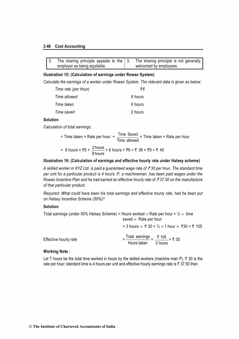
3.46 Cost Accounting
3. The sharing principle appeals to the employer as being equitable.
3. The sharing principle is not generally welcomed by employees.
Illustration 15: (Calculation of earnings under Rowan System)
Calculate the earnings of a worker under Rowan System. The relevant data is given as below:
Time rate (per Hour) `6
Time allowed 8 hours.
Time taken 6 hours.
Time saved 2 hours.
Solution
Calculation of total earnings:
= Time taken × Rate per hour + allowed Time
Saved Time× Time taken × Rate per hour
= 6 hours × `6 + hours 8
hours 2× 6 hours × `6 = ` 36 + `9 = ` 45
Illustration 16: (Calculation of earnings and effective hourly rate under Halsey scheme)
A skilled worker in XYZ Ltd. is paid a guaranteed wage rate of ` 30 per hour. The standard time
per unit for a particular product is 4 hours. P, a machineman, has been paid wages under the
Rowan Incentive Plan and he had earned an effective hourly rate of ` 37.50 on the manufacture
of that particular product.
Required: What could have been his total earnings and effective hourly rate, had he been put
on Halsey Incentive Scheme (50%)?
Solution
Total earnings (under 50% Halsey Scheme) = Hours worked ×Rate per hour + ½ × time
saved × Rate per hour
= 3 hours × ` 30 + ½ ×1 hour × `30 = ` 105
Effective hourly rate =takenHours
earnings Total=
`
105
3 hours= ` 35
Working Note :
Let T hours be the total time worked in hours by the skilled workers (machine man P), ` 30 is the
rate per hour; standard time is 4 hours per unit and effective hourly earnings rate is ` 37.50 then
© The Institute of Chartered Accountants of India

Labour 3.47
Earning (under Rowan plan) = Hours worked × Rate per hr + allowed Time
saved Time×
Time taken × Rate per hr
` 37.5 T = T × `30 + 4
T)(4 − × T × ` 30
` 37.5 = ` 30 + (4 – T) × ` 7.5
or, ` 7.5 T = ` 22.5
or, T = 3 hours.
Illustration 17: (Comparison of earnings between Halsey plan and Rowan plan)
(a) Bonus paid under the Halsey Plan with bonus at 50% for the time saved equals the bonus
paid under the Rowan System. When will this statement hold good? (Your answer should
contain the proof).
(b) The time allowed for a job is 8 hours. The hourly rate is `8. Prepare a statement showing :
i. The bonus earned
ii. The total earnings of labour and
iii. Hourly earnings.
Under the Halsey System with 50% bonus for time saved and Rowan System for each hour
saved progressively.
Solution:
(a) Bonus under Halsey Plan = 100
50 × (SH - AH) × R (i)
Bonus under Rowan Plan : = SH
AH × (SH - AH) × R (ii)
Bonus under Halsey Plan will be equal to the bonus under Rowan Plan when the following
condition holds good :
100
50 × (SH - AH) × R =
SH
AH × (SH - AH) × R
100
50 =
SH
AH
Hence, when the actual time taken (AH) is 50% of the time allowed (SH), the bonus under
Halsey and Rowan Plans is equal.
(b) Statement of Bonus, total earnings of labour and hourly earnings under Halsey and Rowan
Systems.
© The Institute of Chartered Accountants of India

3.48 Cost Accounting
SH
AH Time saved
Basic wages (AH
× `8) (B
× `8)
Bonus under Halsey System
×× 8C100
50
Bonus under Rowan system
×× 8CA
B
Total Earnings
under Halsey System
D+E
Total Earnings
under Rowan System
D+F
Hourly Earnings
under Halsey System
G/B
Hourly Earnings
under Rowan
System H/B
A
hours
B hours C = (A-B) hours
D
`
E
`
F
`
G
`
H
`
I
`
J
`
8
8
8
8
8
8
8
8
8
7
6
5
4
3
2
1
-
1
2
3
4
5
6
7
64
56
48
40
32
24
16
8
-
4
8
12
16
20
24
28
-
7
12
15
16
15
12
7
64
60
56
52
48
44
40
36
64
63
60
55
48
39
28
15
8.00
8.57
9.33
10.40
12.00
14.67
20.00
36.00
8.00
9.00
10.00
11.00
12.00
13.00
14.00
15.00
Illustration 18: (Preparation of Comparison statement of earnings)
Two workmen, ‘A’ and ‘B’, produce the same product using the same material. Their normal wage
rate is also the same. ‘A’ is paid bonus according to the Rowan system, while ‘B’ is paid bonus
according to the Halsey system. The time allowed to make the product is 50 hours. ‘A’ takes 30 hours
while ‘B’ takes 40 hours to complete the product. The factory overhead rate is ` 5 per man-hour
actually worked. The factory cost for the product for ‘A’ is ` 3,490 and for ‘B’ it is ` 3,600.
Required :
(a) Compute the normal rate of wages;
(b) Compute the cost of materials cost;
(c) Prepare a statement comparing the factory cost of the products as made by the two workmen.
Solution:
Step 1 : Let X be the cost of material and Y be the normal rate of wages per hour.
Step 2 : Factory Cost of Workman ‘A’
(`)
A. Material Cost X
B. Wages 30 Y
C. Bonus = SH
AH × (SH - AH) × R 12 Y
Bonus = 50
30 × (50 - 30) × Y
D. Overheads (30 × `5) 150
E. Factory Cost X + 30Y + 12 Y + `150
or, X + 42 Y = `3,490 (Given) – `150 = `3,340 Equation (I)
© The Institute of Chartered Accountants of India

Labour 3.49
Step 3 : Factory Cost of Workman ‘B’
(`)
A. Material Cost X
B. Wages 40 Y
C. Bonus = 50% of (SH - AH) × R 5 Y
= 50% of (50 - 40) × R
D. Overheads (40 × `5) 200
E. Factory Cost X + 40Y + 5 Y + `200
or, X + 45 Y = `3,600 (Given) – `200 = `3,400 Equation (II)
Step 4 : Subtracting Eq. (I) from Eq. (II)
3Y = `60
Y = ` 60/3 = ` 20 per hour.
(a) The normal rate of wages : ` 20 per hour
(b) The cost of material : X + 45 × ` 20 = ` 3,400
X : = ` 3,400 – ` 900 = ` 2,500
(c) Comparative Statement of the Factory Cost of the product made by the two workmen.
‘A’
(`)
‘B’
(`)
Material cost 2,500 2,500
Direct Wages (30 × ` 20) 600 (40 × ` 20) 800
Bonus (12 × ` 20) 240 (5 × ` 20) 100
Factory Overhead 150 200
Factory Cost 3,490 3,600
Illustration 19: (Appropriate incentive scheme)
A factory having the latest sophisticated machines wants to introduce an incentive scheme for
its workers, keeping in view the following:
(i) The entire gains of improved production should not go to the workers.
(ii) In the name of speed, quality should not suffer.
(iii) The rate setting department being newly established are liable to commit mistakes.
You are required to devise a suitable incentive scheme and demonstrate by an illustrative
numerical example how your scheme answers to all the requirements of the management.
© The Institute of Chartered Accountants of India

3.50 Cost Accounting
Solution
Rowan Scheme of premium bonus (variable sharing plan) is a suitable incentive scheme for the
workers of the factory. If this scheme is adopted, the entire gains due to time saved by a worker
will not pass to him.
Another feature of this scheme is that a worker cannot increase his earnings or bonus by merely
increasing its work speed. The reason for this is that the bonus under Rowan Scheme is
maximum when the time taken by a worker on a job is half of the time allowed. As this fact is
known to the workers, therefore, they work at such a speed which helps them to maintain the
quality of output too.
Lastly, Rowan System provides a safeguard in the case of any loose fixation of the standards
by the rate-setting department. It may be observed from the following illustration that in the
Rowan Scheme the bonus paid will be low due to any loose fixation of standards. Workers
cannot take undue advantage of such a situation. The above three features of Rowan Plan can
be discussed with the help of the following illustration:
(i) Time allowed = 4 hours
Time taken = 3 hours
Time saved = 1 hour
Rate = ` 5 per hour
Bonus = allowed Time
taken Time× Time saved × Rate
= hours 4
hours 3 × 1 hour × ` 5 = ` 3.75
In the above illustration time saved is 1 hour and, therefore, total gain is ` 5. Out of ` 5
according to Rowan Plan only ` 3.75 is given to the worker in the form of bonus and the
remaining ` 1.25 remains with the management. In other words a worker is entitled for
75 percent of the time saved in the form of bonus.
(ii) The figures of bonus in the above illustration when the time taken is 2 hours and 1 hour
respectively are as below:
Bonus = allowed Time
taken Time × Time saved × Rate
= hours 4
hours 2× 2 hours × ` 5 = ` 5
= hours 4
hours 1 × 3 hours × ` 5 = ` 3.75
The above figures of bonus clearly show that when time taken is half of the time allowed,
the bonus is maximum. When the time taken is reduced from 2 to 1 hour, the bonus figure
© The Institute of Chartered Accountants of India

Labour 3.51
fell by ` 1.25. Hence, it is quite apparent to workers that it is of no use to increase speed
of work. This feature of Rowan Plan thus protects the quality of output.
(iii) If the rate-setting department erroneously sets the time allowed as 10 hours instead of 4
hours, in the above illustration; then the bonus paid will be as follows:
Bonus = hours 10
hours 3× 7 hours × ` 5 = ` 10.50
The bonus paid for saving 7 hours thus is ` 10.50 which is approximately equal to the wages
of 2 hours. In other words the bonus paid to the workers is low. Hence workers cannot take
undue advantage of any mistake committed by the time setting department of the concern.
3.10.11 Barth System The formula used for calculating the remuneration under this system
is as follows :
Earnings = Hourly rate × workedHours × hours Standard
© The Institute of Chartered Accountants of India

3.52 Cost Accounting
The system is particularly suitable for trainees and beginners and also for unskilled workers. The
reason is that for low production efficiency, the earnings are higher than in the piece-work system
but as the efficiency increases, the rate of increase in the earnings falls.
This system is not suitable for workers having more than 100% efficiency as it does not provide
incentive on working at more than 100% efficiency.
Illustration 20: (Selection of appropriate incentive scheme)
Mr. A. is working by employing 10 skilled workers. He is considering the introduction of some
incentive scheme - either Halsey Scheme (with 50% bonus) or Rowan Scheme - of wage
payment for increasing the labour productivity to cope with the increased demand for the product
by 25%. He feels that if the proposed incentive scheme could bring about an average 20%
increase over the present earnings of the workers, it could act as sufficient incentive for them
to produce more and he has accordingly given this assurance to the workers.
As a result of the assurance, the increase in productivity has been observed as revealed by the
following figures for the current month :
Hourly rate of wages (guaranteed) ` 2.00
Average time for producing 1 piece
by one worker at the previous performance 2 hours
(This may be taken as time allowed)
No. of working days in the month 25
No. of working hours per day for each worker 8
Actual production during the month 1,250 units
Required:
1. Calculate effective rate of earnings per hour under Halsey Scheme and Rowan Scheme.
2. Calculate the savings to Mr. A in terms of direct labour cost per piece under the schemes.
3. Advise Mr. A about the selection of the scheme to fulfill his assurance.
Solution
Working Notes:
1. Total time wages of 10 workers per month:
= No. of working days in the month × No. of working hours per day of each worker ×
Hourly rate of wages × No. of workers
= 25 days × 8 hrs. × ` 2 × 10 workers = ` 4,000
© The Institute of Chartered Accountants of India

Labour 3.53
2. Time saved per month :
Time allowed per piece to a worker 2 hours
No. of units produced during the month by 10 workers 1,250 pieces
Total time allowed to produce 1,250 pieces (1,250 × 2 hours) 2,500 hours
Actual time taken to produce 1,250 pieces 2,000 hours
Time saved (2,500 hours – 2,000 hours) 500 hours
3. Bonus under Halsey scheme to be paid to 10 workers :
Bonus = (50% of time saved) × hourly rate of wages
= 50/100 × 500 hours × ` 2 = ` 500
Total wages to be paid to 10 workers are (` 4,000 + ` 500) ` 4,500, if Mr. A considers
the introduction of Halsey Incentive Scheme to increase the labour productivity.
4. Bonus under Rowan Scheme to be paid to 10 workers:
Bonus = allowed Time
taken Time× Time saved × hourly rate
= 2,000hours
2,500hours× 500 hours × ` 2 = ` 800
Total wages to be paid to 10 workers are (` 4,000 + ` 800) ` 4,800, if Mr. A considers
the introduction of Rowan Incentive Scheme to increase the labour productivity.
1. (i) Effective hourly rate of earnings under Halsey scheme :
(Refer to Working Notes 1, 2 and 3)
= Total time wages of 10 workers+Total bonus under Halsey scheme
Total hours worked
= R` + `
4,000 500
2,000 hours= ` 2.25
(ii) Effective hourly rate of earnings under Rowan scheme :
(Refer to Working Notes 1, 2 and 4)
= Total time wages of 10 workers+Total bonus under Rowan scheme
Total hours worked
= R` +R`
4,000 800
2,000 hours= ` 2.40
© The Institute of Chartered Accountants of India

3.54 Cost Accounting
2. (i) Saving in terms of direct labour cost per piece under Halsey scheme :
(Refer to Working Note 3)
Labour cost per piece (under time wage scheme) = 2 hours × ` 2 = ` 4.
Labour cost per piece (under Halsey scheme)
= Total wages paid under the scheme
Total number of units produced =
` 4,500
1,250= ` 3.60
Saving per piece : (` 4 – ` 3.60) = ` 0.40.
(ii) Saving in terms of direct labour cost per piece under Rowan Scheme:
(Refer to Working Note 4)
Labour cost per piece under Rowan scheme = ` 4,800/1,250 units = ` 3.84
Saving per piece = ` 4 – ` 3.84 = ` 0.16.
3. From the labour cost per piece under Halsey scheme (` 3.60) and Rowan scheme
(` 3.84), it is quite clear that Halsey scheme brings about more saving than Rowan scheme to
the concern. But Halsey scheme does not fulfill the assurance given to the workers about 20%
increase in their earnings as it secures only 12.5% [500/4,000 × 100] increase.
On the other hand, Rowan scheme secures 20% [800/4,000 × 100] increase in the earnings and
it fulfills the assurance. Therefore, Rowan scheme may be adopted.
Illustration 21: (Calculation of earnings under different schemes)
Wage negotiations are going on with the recognised labour union and the Management wants
you as the Cost Accountant of the Company to formulate an incentive scheme with a view to
increase productivity.
The case of three typical workers Achyuta, Ananta and Govida who produce respectively 180, 120
and 100 units of the company’s product in a normal day of 8 hours is taken up for study.
Assuming that day wages would be guaranteed at 75 paise per hour and the piece rate would be
based on a standard hourly output of 10 units, calculate the earnings of each of the three workers
and the labour cost per 100 pieces under (i) Day wages, (ii) Piece rate, (iii) Halsey scheme, and (iv)
The Rowan scheme.
Also calculate under the above schemes the average cost of labour for the company to produce 100
pieces.
Solution
Calculation of earnings of each of the three workers and the labour cost per 100 pieces under
different wage schemes.
© The Institute of Chartered Accountants of India

Labour 3.55
(i) Day wages
Name of workers Day Actual Labour
wages output cost per
(units) 100 pieces
(`) (`)
Achyuta 6.00 180 3.33
Ananta 6.00 120 5.00
Govinda 6.00 100 6.00
Total 18.00 400
Average cost of labour for the company to produce 100 pieces:
output Total
paid wagesTotal × 100 =
18
400
`× 100 = ` 4.50
(ii) Piece rate
Name of workers Actual Piece Wages Labour
output rate earned cost per
(units) (`) (`) 100 pieces
(`)
Achyuta 180 0.075 13.50 7.50
Ananta 120 0.075 9.00 7.50
Govinda 100 0.075 7.50 7.50
Total 400 30.00
Average cost of labour for the company to produce 100 pieces : =` 30
400 × 100 = ` 7.50
(iii) Halsey Scheme
Name of Acutal Std. time Actual Time Bonus Total Labour
workers output for time saved Hrs. wages cost per
(units) actual for Hrs. (50% including 100
output actual of time Bonus* pieces
Hrs. output saved
Hrs. Hrs.) (`) (`)
Achyuta 180 18 8 10 5 9.75 5.42
Ananta 120 12 8 4 2 7.50 6.25
© The Institute of Chartered Accountants of India

3.56 Cost Accounting
Govinda 100 10 8 2 1 6.75 6.75
24.00
Average cost of labour for the company to produce 100 pieces =24
400
` ×100= `6.00
*Total wages = (Actual hours worked + bonus hours) × Rate per hour
Hence total wages of Achyuta are: (8 + 5) × ` 0.75 = ` 9.75
Similarly, the total wages of Ananta and Govinda are ` 7.50 and ` 6.75 respectively.
(iv) Rowan Scheme:
Name of Actual Std. time Actual Time Bonus* Wages for Bonus Total Labour
workers output for time saved hrs. actual @ 75 P earnings cost
(units) actual taken (hours) hrs. per per
output hours @ 75 P Bonus 100
(hrs.) per hr. hour pieces
(`) (`) (`) (`)
(1) (2) (3) (4) (5) (6) (7) (8) (7)+(8)=(9) (10)
Achyuta 180 18 8 10 4.44 6.00 3.33 9.33 5.18
Ananta 120 12 8 4 2.67 6.00 2.00 8.00 6.67
Govinda 100 10 8 2 1.6 6.00 1.20 7.20 7.20
24.53
`
=24.53
Average cos t of labour to the company for 100 pieces400
× 100 = ` 6.13
*Bonus hours = Time taken ×allowed Time
saved Time
Bonus hours of Achyuta = hours 18
hours 10×hours 8 = 4.44
Similarly, bonus hours of Ananta and Govinda are `2.67 hours and `1.6 hours respectively.
3.10.12 Group System of wage payment: Certain jobs or operations are required to be
performed collectively by a number of workers. Under such cases each man’s work depends on
the work performed by one or more of his colleagues and as such it is not possible to measure
separately the output of each worker.
The workers constituting a group or a team here are considered as a composite unit and the
combined output of such a unit is measured for the purpose of wage calculation. The methods
usually used for distributing wages to each worker are the following:
1. Equally, if all the workers of the group are of the same grade and skill, same rate of pay
© The Institute of Chartered Accountants of India
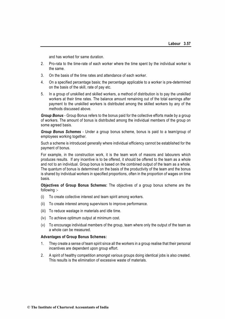
Labour 3.57
and has worked for same duration.
2. Pro-rata to the time-rate of each worker where the time spent by the individual worker is
the same.
3. On the basis of the time rates and attendance of each worker.
4. On a specified percentage basis; the percentage applicable to a worker is pre-determined
on the basis of the skill, rate of pay etc.
5. In a group of unskilled and skilled workers, a method of distribution is to pay the unskilled
workers at their time rates. The balance amount remaining out of the total earnings after
payment to the unskilled workers is distributed among the skilled workers by any of the
methods discussed above.
Group Bonus - Group Bonus refers to the bonus paid for the collective efforts made by a group of workers. The amount of bonus is distributed among the individual members of the group on some agreed basis.
Group Bonus Schemes - Under a group bonus scheme, bonus is paid to a team/group of employees working together.
Such a scheme is introduced generally where individual efficiency cannot be established for the payment of bonus.
For example, in the construction work, it is the team work of masons and labourers which produces results. If any incentive is to be offered, it should be offered to the team as a whole and not to an individual. Group bonus is based on the combined output of the team as a whole. The quantum of bonus is determined on the basis of the productivity of the team and the bonus is shared by individual workers in specified proportions, often in the proportion of wages on time basis.
Objectives of Group Bonus Schemes: The objectives of a group bonus scheme are the following :-
(i) To create collective interest and team spirit among workers.
(ii) To create interest among supervisors to improve performance.
(iii) To reduce wastage in materials and idle time.
(iv) To achieve optimum output at minimum cost.
(v) To encourage individual members of the group, team where only the output of the team as a whole can be measured.
Advantages of Group Bonus Schemes:
1. They create a sense of team spirit since all the workers in a group realise that their personal incentives are dependent upon group effort.
2. A spirit of healthy competition amongst various groups doing identical jobs is also created. This results is the elimination of excessive waste of materials.
© The Institute of Chartered Accountants of India

3.58 Cost Accounting
3. The operators and supervisors also feel interested in raising the production to higher levels.
4. The scheme is usually easier to understand and entails less costing and accounting work. It is easier to set up group activity targets, since the performance unit is large.
Schemes of group bonus - There are five schemes of group bonus as discussed below :
(1) Priestman’s Production Bonus: This method was adopted by Priestman Bros. Ltd., in 1917.
According to this method when the actual production in units or points exceeds the standard fixed, a bonus is paid to the workers as additional wages equivalent to the percentage of actual output over the standard output.
(2) Cost Efficiency Bonus: Under this scheme, the amount of bonus is calculated when the cost is reduced below the normal established targets. Targets of cost, for example, material cost, labour cost and overhead cost etc., per unit are fixed. If the measurement of actual performance shows a saving in the total labour and material cost or a reduction in the total cost per unit, a fair percentage of the saving is distributed among the staff.
Three popular schemes usually used for calculating the amount to be distributed to workers
as Bonus are as below:
(i) Nunn-Bush Plan: According to this plan a norm of direct labour cost is fixed and
expressed as a percentage of the sales value.
The amount calculated at this percentage is credited to a fund. The actual labour cost
is debited to this fund and the balance remaining to the credit of this fund is distributed
as bonus to all the workers and employees.
(ii) Scanlon Plan: Here also a fund is created for the normal cost of wages and salaries.
This fund is debited with the actual labour costs. Two-thirds to three-fourths of the
credit balance, if any, is distributed as bonus, the balance is kept as reserve for future
set-backs.
(iii) Rucker Plan: This plan is quite similar to Nunn-Bush Plan except that the percentage
for crediting the fund is based on the total value added by manufacturer (i.e. the total
cost less the value of the material) and not on total sales value.
(3) Town Gain Sharing Plan: Under this plan bonus is dependent upon a saving in the labour
cost as compared to standard. The bonus is calculated at 50% of the saving achieved.
(4) Budgeted Expense Bonus: Bonus is determined in advance and paid as a percentage of
savings effected in the actual total expenses as compared to the budgeted expense. It is
payable to indirect workers also.
(5) Waste Reduction Bonus: Bonus becomes payable under this scheme if the team of
workers brings about a reduction in the percentage of material wastages as compared to
the standard set. It is applicable to industries where the material cost assumes a greater
proportion of the total cost.
© The Institute of Chartered Accountants of India

Labour 3.59
Many times group bonus schemes do not enjoy the approval of workers. Some workers tend to
feel that their personal incentives are low merely because some members of the group are lazy
or inefficient. Such workers believe that it is better to provide incentives on individual basis, if it
is possible.
3.10.13 System of Incentive schemes for Indirect Workers: Since the setting of work
standards and measurement of output in the case of indirect workers is not an easy task in
respect of maintenance, internal transport, inspection, packing and cleaning, therefore the intro-
duction of a system of payment by results for indirect workers is difficult.
In spite of the aforesaid difficulty, it has been felt necessary to provide for incentives to indirect
workers, due to the following reasons:
1. Dissatisfaction: Payment of incentive bonus to direct workers and time rate to indirect
workers leads to dissatisfaction and labour unrest.
2. Entitlement: Indirect workers are as much entitled to bonus as direct workers.
3. Team Spirit: Bonus payment to indirect workers creates team spirit.
4. Increase in efficiency: An incentive system for indirect workers assists in maintaining the
efficiency of services such as plant repairs, stores maintenance, material handling etc.
5. Dependence on indirect labour: The efficiency of direct workers is reduced where their
work is dependent upon the service rendered by the indirect workers.
A few examples of incentive schemes to indirect workers are as below :
(i) Incentive to supervisors and foremen: Supervisors and foremen are an important link
between the management and the workers. Incentive payment to these persons would
assist in maintaining all round efficiency. Incentive to supervisors and foremen may be
provided in the form of non-financial benefits.
Incentive can also be provided to these workers in the form of Bonus. The extent of bonus
which will be distributed as incentive will depend on the savings effected over the
standards.
(ii) Incentive to maintenance and repairs staff: Under mass production work, repair and
maintenance duties can be considered as routine and repetitive for which percentage of
efficiency can be evaluated. In case such an evaluation is not possible or practicable, a
group bonus system may be established, on the basis of reduction in breakdown or on the
number of complaints.
Illustration 22: (Calculation of earnings of each worker under group task)
A, B and C were engaged on a group task for which a payment of ` 725 was to be made. A’s
time basis wages are ` 8 per day, B’s ` 6 per day and C’s ` 5 per day. A worked for 25 days;
B worked for 30 days; and C for 40 days. Distribute the amount of ` 725 among the three
workers.
© The Institute of Chartered Accountants of India

3.60 Cost Accounting
Solution
Total wages on time basis: (`)
A 25 @ ` 8 200
B 30 @ ` 6 180
C 40 @ ` 5 200
580
Payment for the task
Bonus : (` 725 – ` 580) 145
or, 25% of the time-basis wages. 725
Earnings of each worker
Worker Wages on time basis Group task Bonus 25% Total
(`) (`) (`)
A 200 50 250
B 180 45 225
C 200 50 250
580 145 725
Illustration 23: (Calculation of bonus earned by direct and indirect labour)
Both direct and indirect labours of a department in a factory are entitled to production bonus in
accordance with a group incentive scheme, the outline of which is as follows:
(a) For any production in excess of the standard rate fixed at 16,800 tonnes per month (of 28
days) a general incentive of ` 15 per tonne is paid in aggregate. The total amount payable
to each separate group is determined on the basis of an assumed percentage of such
excess production being contributed by it, namely @ 65% by direct labour, @ 15% by
inspection staff, @ 12% by maintenance staff and @ 8% by supervisory staff.
(b) Moreover, if the excess production is more than 20% above the standard, direct labour
also get a special bonus @ ` 5 per tonne for all production in excess of 120% of standard.
(c) Inspection staff are penalized @ ` 20 per tonne for rejection by customer in excess of 2%
of production.
(d) Maintenance staff are also penalized @ ` 20 per hour for breakdown.
From the following particulars for a month, work out production bonus earned by each group :
(a) Actual working days : 25
(b) Production : 21,000 tonnes
(c) Rejection by customer : 500 tonnes
(d) Machine breakdown : 40 hours
© The Institute of Chartered Accountants of India

Labour 3.61
Solution
1. Standard output per day = month a in days of number Budgeted
month peroutput Standard
= days 28
tonnes 16,800 = 600 tonnes
2. Standard output for 25 days = 600 tonnes × 25 days = 15,000 tonnes
(a) General Incentive
(i) Standard output : 15,000 tonnes (ii) Actual output : 21,000 tonnes
(iii) Excess output over standard : 21,000 – 15,000 = 6,000 tonnes
(iv) Percentage of excess : 40%
production to standard output : 6,000 tonnes
15,000 tonnes × 100
(v) Aggregate general incentive : = Excess output × ` 15
: = 6,000 tonnes × `15 = ` 90,000
(vi) Allocation of general incentive
Direct labour : 65% of ` 90,000 ` 58,500
Inspection staff : 15% of ` 90,000 ` 13,500
Maintenance staff : 12% of ` 90,000 ` 10,800
Supervisory staff : 8% of ` 90,000 ` 7,200
Total ` 90,000
(b) Special bonus to direct workers
(i) 20% is the excess output over 120% of standard output
or 3,000 tonnes (15,000 tonnes × 20%)
(ii) Special incentive = 3,000 tonnes × ` 5 = ` 15,000
(c) Penalty imposed on inspection staff
(i) Normal rejection = 2% of production = 2% of 21,000 tonnes
= 420 tonnes
(ii) Actual rejection = 500 tonnes
(iii) Excess rejection over normal rejection = 500 – 420 = 80 tonnes
(iv) Penalty = 80 tonnes × ` 20 per tonne = ` 1,600
© The Institute of Chartered Accountants of India

3.62 Cost Accounting
(d) Penalty imposed on maintenance staff
(i) Breakdown hours = 40 hours
(ii) Penalty = 40 hours × ` 20 per hour = ` 800
Statement of production bonus earned by each group
Particulars Direct Inspection Maintenance Supervisory Total
labour staff staff staff
(`) (`) (`) (`) (`)
1 2 3 4 5
Aggregate
general incentive 58,500 13,500 10,800 7,200 90,000
Special bonus 15,000 - - - 15,000
Penalty - (1,600) (800) - (2,400)
Production bonus 73,500 11,900 10,000 7,200 1,02,600
3.10.14 Profit-sharing and Co-partnership schemes: A profit-sharing scheme implies
that the net profit of business would be shared between the workers and the shareholders or
the partners in a pre-determined ratio.
Co-partnership, on the other hand, implies that the workers shall own the business jointly with
the shareholders. In this case, usually the workers share of profits is given in the form of shares.
Some employers in our country originally introduced profit-sharing schemes with a view of
stimulating interest among workers for increasing production. But the schemes have not been
successful on account of unwillingness on the part of the management to consult workers. Even
a demand for copies of final accounts of the business to be shown to them has been considered
by some employers to be an unwarranted interference. The question of bonus has thus been
one of the major causes of industrial disputes in recent years. (Payment of compulsory bonus
is now governed by the payment of Bonus Act.)
Though profit sharing has become a normal feature of the industrial life in this country, co-
partnership is comparatively unknown. Nevertheless it must be pointed out that in England and
other Western countries, a number of successful concerns have been allotting shares to their
workers in proportion to their shares of bonus. Some of them have advanced loans to them to
purchase shares. Both these forms of benefit have been quite popular with labour.
Advantages Disadvantages
(i) Employees are made to feel that they too have a stake in the well-being of the undertaking and have a contribution to make in earning of profits by improving production, efficiency and operations.
(i) Profit may fluctuate from year to year; there is thus an element of uncertainty in such schemes.
(ii) Profit depends upon many factors of which labour efficiency is only one.
© The Institute of Chartered Accountants of India

Labour 3.63
(ii) Labour turnover may be reduced, particularly if a minimum period of service is laid down as a condition for participating in such schemes.
(iii) Better team work and better co-operation.
Insufficiency of bonus may lead to dissatisfaction instead of promoting good relations, if the good work done by labour is nullified by other factors.
(iii) The reward may be too remote to sustain continued interest in and zeal for work.
(iv) There may be doubt and suspicion about the profit disclosed.
(v) Since all are entitled to participate in such schemes, there is no recognition of individual merit.
(vi) The individual share of profit may be too meagre to be appealing.
(vii) Since in practice bonus has to be fought in India, so it has become an important cause of labour disputes.
Workers share in the net profits of the firm can be calculated by any of the following ways:
(i) A fixed percentage may be allowed to the worker as bonus at the end of the financial year.
(ii) The profit earned, can be department wise and hence a fixed percentage of the department’s
profit can be allowed as profit sharing.
(iii) Profits may be computed per unit of output and a part of profit may be allowed to workers
on this basis.
Treatment in Costing: In foreign countries bonus is an ex-gratia payment and hence it is
regarded as an appropriation of profit not to be included in costs. In fact trade unions there do
not look upon bonus with favour.
In India however, payment of bonus is compulsory under the Payment of Bonus Act under which
8.33% of wages earned or ` 100 whichever is higher, is the minimum bonus payable, the
maximum being 20%. Hence bonus must be treated as part of costs in India.
There can be two methods of dealing with bonus:
(i) It may be treated as part of overheads; in any case, this must be so for bonus paid to
indirect workers.
(ii) In the case of direct workers the bonus payable may be estimated beforehand and wage
rates for costing purposes suitably inflated by including the bonus that would be paid.
Example: A worker gets ` 800 p.m. as wages and it is expected that he will be paid two months’
wages as bonus. His total earning will be ` 11,200 (` 9,600 + ` 1,600). If the worker works for
2,400 hours in a year the wage rate for costing purposes will be: ` 4.67, i.e.,
` 11,200/2,400 hours.
© The Institute of Chartered Accountants of India

3.64 Cost Accounting
Illustration 24: (Calculation and verification of wages paid to the worker)
During audit of account of G Company, your assistant found errors in the calculation of the
wages of factory workers and he wants you to verify his work.
He has extracted the following information:
(i) The contract provides that the minimum wage for a worker is his base rate. It is also paid
for downtimes i.e., the machine is under repair or the worker is without work. The standard
work week is 40 hours. For overtime production, workers are paid 150 percent of base
rates.
(ii) Straight Piece Work – The worker is paid at the rate of 20 paise per piece.
(iii) Percentage Bonus Plan – Standard quantities of production per hour are established by
the engineering department. The workers’ average hourly production, determined from his
total hours worked and his production, is divided by the standard quantity of production to
determine his efficiency ratio. The efficiency ratio is then applied to his base rate to
determine his hourly earnings for the period.
(iv) Emerson Efficiency Plan – A minimum wages is paid for production upto 66-2/3% of
standard output or efficiency. When the workers production exceeds 66-2/3% of the
standard output, he is paid bonus as per the following table:
Efficiency Level Bonus
Upto 663
2% Nil
663
2% to 79 % 10%
80% – 99% 20%
100% – 125% 45%
Your assistant has produced the following schedule pertaining to certain workers of a
weekly pay roll:
Workers Wage Incentive Total Down Units Standard Base Gross
Plan Hours Time Produced Units Rate Wages
Hours as per
Book
` `
Rajesh Straight piece work 40 5 400 — 1.80 85
Mohan* Straight piece work 46 — 455 — 1.80 95
John Straight piece work 44 — 425 — 1.80 85
Harish Percentage bonus plan 40 4 250 200 2.20 120
© The Institute of Chartered Accountants of India

Labour 3.65
Mahesh Emerson 40 — 240 300 2.10 93
Anil Emerson 40 — 600 500 2.00 126
(40 hours production)
* Total hours of Mohan include 6 overtime hours.
Prepare a schedule showing whether the above computation of workers’ wages are correct
or not. Give details.
Solution
Schedule showing the correct figure of
minimum wages, gross wages and wages to be paid
Workers Wage Minimum Gross wages Gross wage Wages to be paid
incentive wages computed as per as per book are Maximum of :
plan Incentive plan minimum and
gross computed
wages
(`) (`) (`) (`)
Rajesh Straight piece work 72.00 80.00 85 80.00
(Refer to W. Note 1)
Mohan Straight piece work 88.20 91.00 95 91.00
(Refer to W. Note 2)
John Straight piece work 82.80 85.00 85 85.00
(Refer to W. Note 3)
Harish Percentage bonus plan 88.00 122.00 120 122.00
(Refer to W. Note 4)
Mahesh Emerson 84.00 100.80 93 100.80
(Refer to W. Note 5)
Anil Emerson 80.00 116.00 126 116.00
(Refer to W. Note 6)
Working notes :
1. Minimum wages = Total normal hours × rate per hour
= 40 hours × ` 1.80 = ` 72
Gross wages (computed) = No. of units × rate per unit
as per incentive plan = 400 units × ` 0.20 = ` 80
2. Minimum wages = Total normal hours × Rate per hour + Overtime hours × Overtime rate per hour
= 40 hours × ` 1.80 + 6 hours × ` 2.70
= ` 72 + ` 16.20 = ` 88.20
Gross wages (computed) = 455 units × ` 0.20 = ` 91.00
as per incentive plan
© The Institute of Chartered Accountants of India

3.66 Cost Accounting
3. Minimum wages = 40 hours × ` 1.80 + 4 hours × ` 2.70
= ` 72 + ` 10.80 = ` 82.80
Gross wages (computed) = 425 units × ` 0.20 = ` 85
as per incentive plan
4. Minimum wages = 40 hours × ` 2.20 = ` 88
Efficiency of worker = Actual production per hour
Standard production per hour× 100
= (250 units/36 hours)
(200 units/40 hours)× 100 = 138.89%
Hourly rate = Rate per hour × Efficiency of worker
= ` 2.20 × 138.89% = ` 3.05
Gross wages (computed)
as percentage of bonus plan = 40 hours × ` 3.05 = ` 122/-
5. Minimum wages = 40 hours × ` 2.10 = ` 84
Efficiency of worker = hours) units/40 (300
hours) units/40 (240 × 100 = 80%
Bonus (as per Emerson’s plan) = Total minimum wages × Bonus percentage
= ` 84 × 20% = ` 16.80
Gross wages (computed) as per
Emerson’s Efficiency plan = Minimum wages + Bonus
= ` 84 + ` 16.80 = ` 100.80
6. Minimum wages = 40 hours × ` 2 = ` 80
Efficiency of worker = 500
600× 100 = 120%
Bonus (as per Emerson’s plan) = ` 80 × 45% = ` 36
Gross wages (computed) as per
Emerson’s Efficiency plan = ` 80 + ` 36 = ` 116
Illustration 25: (Evaluation of proposal)
The present output details of a manufacturing department are as follows:
Average output per week 48,000 units from 160 employees
Saleable value of output ` 6,00,000
© The Institute of Chartered Accountants of India

Labour 3.67
Contribution made by output
towards fixed expenses and profit ` 2,40,000
The Board of Directors plans to introduce more mechanisation into the department at a capital
cost of ` 1,60,000. The effect of this will be to reduce the number of employees to 120, and
increasing the output per individual employee by 60%. To provide the necessary incentive to
achieve the increased output, the Board intends to offer a 1% increase on the piece work rate
of ` 1 per unit for every 2% increase in average individual output achieved.
To sell the increased output, it will be necessary to decrease the selling price by 4%.
Calculate the extra weekly contribution resulting from the proposed change and evaluate for the
Board’s information, the desirability of introducing the change.
Solution
1. Present average output per employee and total future expected output per week
Present average output per employees per week = employeespresent of number Total
outputpresent Total
= employees 160
units 48,000= 300 units
Total Future expected output per week = Total number of future employees
(present output + 60% of present
output per employee)
= 120 employees (300 units + 60% ×
300 units)
= 57,600 units
2. Present and proposed piece work rate
Present piece work rate = ` 1.00 per unit
Proposed piece work rate = Present piece work rate + 30% × ` 1
= ` 1.00 + 0.30 P
= ` 1.30 per unit
3. Present and proposed sale price per unit
Present sales price per unit = ` 12.50
(` 6,00,000/48,000 units)
Proposed sale price per unit = ` 12
(` 12.50 – 4% × ` 12.50)
© The Institute of Chartered Accountants of India

3.68 Cost Accounting
4. Present marginal cost (excluding wages) per unit :
= (units)output Present
gespresent wa towards onContributiprofit&expenses Fixedvalue salesPresent −−
= ` ` `
− −6,00,000 2,40,000 48,000
48,000 units = ` 6.50 per unit
Statement of extra weekly contribution
(Information resulting from the proposed change
of mechanisation meant for Board’s evaluation)
Expected sales units 57,600
(Refer to Working note 1)
(`) (`)
Sales value : (A) (57,600 units × ` 12) 6,91,200
(Refer to Working note 3)
Marginal costs (excluding wages) : (B) (57,600 units × ` 6.50) 3,74,400
(Refer to Working note 4)
Wages : (C) (57,600 units × ` 1.30) 74,880
(Refer to Working note 2)
Total marginal cost : (D) = {(B) – (C)} 4,49,280
Marginal contribution : {(A) – (D)} 2,41,920
Less : Present contribution 2,40,000
Increase in contribution (per week) 1,920
Evaluation: Since the mechanisation has resulted in the increase of contribution to the extent of
` 1,920 per week, therefore the proposed change should be accepted.
We have examined the advantages and disadvantages of various methods of remunerating
labour, so we can summarise below that the best method of remuneration can be adjudged
through the following points:
1. A minimum wage should be guaranteed to all workers.
2. Efficient workers are given incentives in the form of bonus so that they can work harder
and produce more.
A share in profits of the firm is given to workers in addition to the minimum wages and bonus
3.11 Absorption of Wages
3.11.1 Elements of wages: In common parlance, the term ‘wages’ represents monetary
payment which an employee receives at regular intervals for the services rendered. Strictly
speaking, however, from the point of view of the employer and the cost to the industry, wages
© The Institute of Chartered Accountants of India

Labour 3.69
should be taken to include also non-monetary benefits which an employee receives by virtue of
employment. Such non-monetary benefits may include:
(i) Medical facilities;
(ii) Educational and training facilities;
(iii) Recreational and sports facilities;
(iv) Housing and social welfare; and
(v) Cost of subsidised canteen and co-operative societies.
Such benefits are generally given in an industrial establishment. In some cases the provision of
benefits is compulsory. Therefore, while computing the wage cost per worker, the monetary
value of such non-monetary benefits should also be taken into account.
The monetary part of a worker’s remuneration includes the basic wages, dearness allowance,
overtime wages, other special allowance, if any, production bonus, employer’s contribution to
the provident fund, Employees State Insurance scheme premium, contribution to pension fund,
leave pay, etc.
The basic wage is the payment for work done, measured in terms of hours attended or the units
produced, as the case may be. The basic wage rate is not normally altered unless there is a
fundamental change in the working conditions or methods of manufacture.
Dearness allowance is an allowance provided to cover the increase in cost of living from one
period to another. This allowance is calculated either as percentage of the basic wage or as a
fixed amount for the days worked. In either case, the percentage or the fixed amount is subject
to revision whenever the cost of living index or consumer price Index rises or falls by a certain
figure as agreed to by the employer with the labour union. When permanent rise in the cost of
living index occurs, a part of the dearness allowance is often absorbed in the basic wage.
Overtime allowance is an allowance paid for the extra hours worked at the rates laid down in
the Factories Act. In certain industries, where special allowance for the working conditions, tool
maintenance, etc., are paid they are also considered as part of wages.
Production Bonus is an incentive payment made to workers for efficiency that results in
production above the standard. There are different methods of computing incentives. Under the
Payment of Bonus Act, a worker is entitled to compulsory bonus of 8.33% wages earned in the
relevant year or ` 100 (whichever is greater). The bonus may be upto 20% of wages depending
upon the quantum of profits calculated as per the Act.
3.11.2. Component of wages cost or wages for costing purposes: In addition to
wages (including allowances, such as D.A.) that are paid to workers, a firm may have to spend on many other items (such as premium to the ESI or provident fund or bonus).
Further, the worker does not spend all the time for which he is paid on productive work.
This is because he is entitled to weekly holiday and various type of leave. There is also a certain amount of unavoidable idle time. The question is to what extent such additional payment or cost
© The Institute of Chartered Accountants of India

3.70 Cost Accounting
in respect of labour can be charged directly to unit of cost as part of direct labour cost? Of course, in the case of indirect labour, all such payments as also the wages paid to them, must be treated as part of overheads.
But in the case of direct workers, two alternatives are possible. The additional charges may be treated as overheads. Alternatively, the wage rates being charged to job may be computed by including such payments; automatically then, such payments will be charged to the work done alongwith wages of the worker. (It should be remembered that such wage rate will be only for costing purposes and not for payment to workers). The total of wages and additional payment should be divided by effective hours of work to get such wage rates for costing purposes.
Illustration 26: (Calculation of wage rate per hour)
A worker is paid `1000 per month and a dearness allowance of ` 200 p.m. Worker contribution to
provident fund is @ 10% and employer also contributes the same amount as the employee. The
Employees State Insurance Corporation premium is 6.5% of wages of which 1.75% is paid by the
employees. It is the firm’s practice to pay 2 months’ wages as bonus each year.
The number of working days in a year are 300 of 8 hours each. Out of these the worker is
entitled to 15 days leave on full pay. Calculate the wage rate per hour for costing purposes.
Solution (`)
Wages paid to worker during the year (` 1,000 +200) x 12 14,400
Add: Employer Contribution to:
Provident Fund @ 10% 1,440 E.S.I. Premium 4.75% (6.5 – 1.75) 684
Bonus at 2 months’ wages (Basic + DA) 2,400
Total 18,924 Effective hours per year: 285 × 8 = 2,280
Wage-rate per hour (for costing purpose): ` 18,924/2,280 hours = `8.30
Illustration 27: (Treatment of abnormal idle time)
In a factory working six days in a week and eight hours each day, a worker is paid at the rate of ` 100 per day basic plus D.A. @ 120% of basic. He is allowed to take 30 minutes off during his
hours shift for meals-break and a 10 minutes recess for rest. During a week, his card showed
that his time was chargeable to :
Job X 15 hrs.
Job Y 12 hrs.
Job Z 13 hrs.
The time not booked was wasted while waiting for a job. In Cost Accounting, how would you
allocate the wages of the workers for the week?
© The Institute of Chartered Accountants of India

Labour 3.71
Solution
Working notes:
(i) Total effective hours in a week :
[(8 hrs. – (30 mts. + 10 mts.)] × 6 days = 44 hours
(ii) Total wages for a week :
(` 100 + 120% of ` 100) × 6 days = ` 1,320
(iii) Wage rate per hour : = ` 30
(iv) Time wasted waiting for
job (Abnormal idle time): = 44 hrs. – (15 hrs. + 12 hrs. + 13 hrs.)
= 4 hrs.
Allocation of wages in Cost Accounting
(`)
Allocated to Job X : 15 hours × ` 30 = 450
Allocated to Job Y : 12 hours × ` 30 = 360
Allocated to Job Z : 13 hours × ` 30 = 390
Charged to Costing Profit & Loss A/c : 4 hours × ` 30 = 120
Total 1,320
3.11.3 Holiday and leave wages: One alternative to account for wages paid on account of
paid holiday and leave can be to include them as departmental overheads. In such a case, it is
necessary to record such wages separately from “worked for wages”. Such a segregation can
be made possible by providing a separate column in the payroll for holiday and leave wages in
the same way as there are columns for dearness allowance, provident fund deductions, etc. If,
however, a separate or additional column cannot be provided for this purpose it would be
necessary to analyse the payroll periodically to ascertain how much of the total payment pertains
to “worked for wages” and how much is attributed to leave and holiday wages.
Another way could be to inflate the wage rate for costing purposes to include holiday and leave
wages. This can be done only in the case of direct workers.
Illustration 28: (Calculation of leave wages)
Calculate the labour hour rate of a worker X from the following data :
Basic pay ` 1,000 p.m.
D.A. ` 300 p.m.
Fringe benefits ` 100 p.m.
Number of working days in a year 300. 20 days are availed off as holidays on full pay in a year.
Assume a day of 8 hours.
© The Institute of Chartered Accountants of India

3.72 Cost Accounting
Solution
(a) (i) Effective working days in a year 300
Less : Leave days on full pay 20
Effective working days 280 days
Total effective working hours (280 days × 8 hours) 2,240
(ii) Total wages paid in a year (`)
Basic pay 12,000
D.A. 3,600
Fringe benefits 1,200
16,800
(iii) Hourly rate : ` 16,800/2,240 hours ` 7.50
3.11.4 Night shift allowance: In some cases, workers get extra payment if they work at
night. Since the extra payment is not for any particular job, therefore such a payment should be
treated as part of overheads.
3.11.5 Principles of remuneration: The term ‘remuneration’ has been defined as the
reward for labour and service. It is the result of the agreement between the employer and the
employee, whereby for a specified work or service rendered by the employee the employer
agrees to pay a specified sum of money. Apart from this an employee by virtue of the fact that
he is an employee becomes entitled to certain non-monetary benefits.
The method of remuneration adopted varies from industry to industry and, in certain cases, even
among different units in the same industry. Whatever be the variation, the method of fixing
remuneration payable to the various categories of employees has to be based on certain
accepted principles. These are:
(i) Geographical Area Based: Wage-rates in an industry should be fixed in conformity with
the general wage-levels in the geographical area i.e. the rate should be more or less the
same for similar efforts and skill. The wage-level in an area would in turn depend upon
demand for labour, the availability of labour, the cost of living in the area, the wage levels
in neighbouring industrial area, and the capacity of the particular industry to pay.
(ii) Performance\Job Based: Wage-rates should be related to the degree of skill, effort, initiative
and responsibility that the employee is expected to assume in respect of the various jobs he
may be called upon to perform. There should be generally equal pay for equal work.
(iii) Minimum Wages: Wage-rates should guarantee a minimum wage regardless of the
existence of factors listed under (ii) above, particularly when the working conditions are
difficult and dangerous.
(iv) Maintain Standard of living: Wage-rates are considered satisfactory only if they enable
the workers to maintain a reasonable standard of living.
© The Institute of Chartered Accountants of India

Labour 3.73
(v) Separate wage rates for different classes of employees: Separate wage rates should
be fixed for different classes of employees since each class expects to maintain a different
standard of living; also the education, physical and mental efforts and responsibility
required for performing different jobs are not the same.
(vi) Incentive as per output: It should be possible for worker to increase his earnings through
extra effort and by increasing output. If he alone is responsible, he should have the full
benefit of the increased productivity. Otherwise, if increased output has resulted from co-
operation between management and workers both should share the benefit.
It is important that these basic principles should be recognised in fixing the wage rate of workers;
otherwise, there will be dissatisfaction among the employees and, consequently, there will be
higher labour turnover. Satisfactory employer-employee relationship is a primary necessity for
industrial development and this has to be ensured to a very great degree, by satisfactory
schemes of remunerating labour.
The aim should be to keep labour cost per unit of output (or service) as low as possible. It is not
the same as keeping wages at low levels.
There is a definite correlation between wages and productivity; high wages often lead to such an
increase in productivity that wages per unit of output fall. However, this rule is also subject to diminishing
returns—a point is reached at which any further increase in wage rates does not bring about a
corresponding increase in efficiency. But generally, higher wages result in lower cost per unit.
Wages affect the national economy through cost of goods produced. If an increase in wages
outpaces the corresponding increase in productivity, goods become costlier and cannot
compete with those of other countries in the world markets.
From the point of view of an expert it is necessary to keep wages in check like other costs. The
safe rule is to link up wages with productivity.
3.11.6 Absorption rates of labour cost: Labour cost as stated above include monetary
compensation and non-monetary benefits to workers.
Monetary benefits include, basic wages, D.A., overtime pay, incentive or production bonus
contribution to employee provident fund, House Rent Allowance, Holiday and vacation pay etc.
The non-monetary benefits include medical facilities, subsidized canteen services, subsidized
housing, education and training facilities.
Accounting of monetary and non-monetary benefits to indirect workers does not pose any
problems because the total of monetary and non-monetary benefits are treated as overhead
and absorbed on the basis of rate per direct labour hour, if overheads are predominantly labour
oriented.
For direct workers, the ideal method is to charge jobs or units produced by supplying per hour
rate calculated as below :
© The Institute of Chartered Accountants of India

3.74 Cost Accounting
Rate per hour = time idle Normal - hours labourdirect Budgeted
benefitsmonetary -non ofcost and benefitsmonetary estimated of otalT
Another alternative method is to treat the monetary benefits other than basic wages and
dearness allowance as well as cost of non-monetary benefits as overheads.
3.12 Efficiency Rating Procedures
Efficiency is usually related with performance and may be computed by comparing the time
taken with the standard time allotted to perform the given job/task.
If the time taken by a worker on a job equals or less than the standard time, then he is rated efficient.
In case he takes more time than the standard time he is rated as inefficient.
Efficiency in % = 100taken Time
std. per as allowed Time×
For efficiency rating of employees the following procedures may be followed:
1. Determining standard time/performance standards: The first step is to determine the
standard time taken by a worker for performing a particular job/task. The standard time can be
determined by using Time & Motion study or Work study techniques. While determining the
standard time for a job/task a heterogeneous group of workers is taken and contingency
allowances are added for determining standard time.
2. Measuring Actual Performance of workers: For computing efficiency rating it is
necessary to develop a procedure for recording the actual performance of workers. The system
developed should record the output of each worker along with the time taken by him.
3. Computation of efficiency rating: The efficiency rating of each worker can be computed
by using the above mentioned Formula.
3.12.1 Need for efficiency rating
1. As discussed earlier when a firm follows a system of payment by results, the payment has a direct relationship with the output given by a worker. The firm for making payment to worker is required to ascertain his efficiency level. For instance, under Taylor's differential piece work system the lower rate i.e. 83% of piece rate is given to a worker when his efficiency rating is less than 100% and higher rate viz., 125% of piece rate is offered at efficiency level of either 100% or more. Similarly under Emersion efficiency plans bonus is paid at rising scale at various level of efficiency, ranging from 66.67% to 150%.
2. The efficiency rating also helps the management in preparing labour requirement budget
or for preparing manpower requirements. For example, let P Ltd. manufactures two
products by using one grade of labour. The following estimates are available :
© The Institute of Chartered Accountants of India

Labour 3.75
Product A Product B
Budgeted production (units) 3,480 4,000
Std. hrs. allowed per product 5 4
It is further worked out that the efficiency rating (efficiency ratio) for productive hours worked by direct workers in actually manufacturing the production is 80% then the exact standard labour requirement can be worked out as follows:
Product A Product B Total
Budgeted production (in units) 3,480 4,000
Std. hours allowed for 17,400 16,000 33,400
budgeted production (3,480 units × 5 hours) (4,000 units × 4 hours)
Since efficiency ratio is given as 80% therefore Std. labour hours required for 100%
efficiency level are
×
80
100hours 400,33 = 41,750 hours.
Labour productivity : Productivity is generally determined by the input/output ratio. In the case
of labour it is calculated as below:
Standard time for doing actual amount of work
Actual time taken to do work
Labour productivity is an important measure for measuring the efficiency of individual workers. It is an index of efficiency and a sign of effectiveness in the utilisation of resources-men, materials, capital, power and all kinds of services and facilities.
It is measured by the output in relation to input. Productivity can be improved by reducing the input for a certain quantity or value of output or by increasing the output from the same given quantity or value of input.
Factors for increasing labour productivity: The important factors which must be taken into consideration for increasing labour productivity are as follows:
1. Employing only those workers who possess the right type of skill.
2. Placing a right type of man on the right job.
3. Training young and old workers by providing them the right types of opportunities.
4. Taking appropriate measures to avoid the situation of excess or shortage of labour at the shop floor.
5. Carrying out work study for the fixation of wage rate, and for the simplification and standardisation of work.
© The Institute of Chartered Accountants of India

3.76 Cost Accounting
3.13 Summary
• Labour Cost: Cost incurred for hiring of human resource of employees
• Direct Labour: Any Labour Cost that is specifically incurred for or can be readily charged
to or identified with a specific job, contract, work order or any other unit of cost.
• Idle Time: The time for which the employer pays but obtains no direct benefit or for no
productive purpose.
• Normal Idle Time: Time which cannot be avoided or reduced in the normal course of
business. The cost of normal idle time should be charged to the cost of production.
• Abnormal Idle Time: It arises on account of abnormal causes and should be charged to
Costing Profit and Loss account.
• Time Keeping: It refers to correct recording of the employees attendance time
• Time Booking: It is basically recording the details of work done and the time spent by
workers on each job or process.
• Overtime: Payment to workers, when a worker works beyond the normal working hours.
Usually overtime has to be paid at double the rate of normal hours.
• Overtime Premium: It’s the amount of extra payment paid to a worker under overtime.
• Labour Turnover: It is the rate of change in labour force during a specified period due to
resignation, retirement and retrenchment. If the labour turnover is high, it’s a sign of
instability and may affect the profitability of the firm.
• Labour turnover can be measured through the following methods:
(i) Replacement Method: Number of employees replaced
×100Average number of employees on roll
(ii) Separation Method: Number of employees separated during the year
×100Average number of employees on rolls during the period
(iii) Flux Method: Number of employees separated + number of employees replaced
×100Average number of employees on rolls during the period
(iv) Labour turnover due to new recruitment:
No. of new workers joining in a period (excluding replacements)
Average number of workers on the roll in a period
© The Institute of Chartered Accountants of India

Labour 3.77
(v) Labour turnover including accessions:
No. of new workers joining in a period (excluding replacements)
Average number of workers on the roll in a period
OR
No. of separations + No. of accessions ×100
Average number of workers
• Incentives: It is the simulation for effort and effectiveness by offering monetary
inducement or enhanced facilities.
• Time Rate System: The amount of wages due to a worker are arrived at by multiplying the
time worked by the appropriate time rate.
• Differential Time Rate: Different hourly rates are fixed for different levels of efficiency.
Upto a certain level a fixed rate is paid and based on the efficiency level the hourly rate
increases gradually.
• Straight Piece Work: Payment is made on the basis of a fixed amount per unit of output irrespective
of time taken. It is the number of units produced by the worker multiplied by rate per unit.
• Differential Piece Rate: For different level of output below and above the standard,
different piece rates are applicable.
(i) Taylor’s Differentials Piece Work system:
Output/ Efficiency Rate
< 100% 83% of normal rate
≥ 100% 125% of normal rate or 150% of lower rate
(ii) Merrick Differential Piece Work System:
Efficiency Piece rate applicable
Upto 83% Normal rate,
Above 83% and upto 100% 10% above normal rate.
Above 100% 20% or 30% above normal rate.
• Gantt Task and bonus system
Output Payment
Output below standard guaranteed time rate.
© The Institute of Chartered Accountants of India

3.78 Cost Accounting
Output at standard Time rate plus bonus of 20% (usually) of time rate.
Output above standard High piece rate on worker’s whole output.
It is so fixed, so as to include a bonus of 20% of the time rate
• Emerson’s Efficiency system:
Efficiency Payment
<66.67% Hourly Rate
66.67%-100% Bonus varies from 1% to 20%
≥ 100% Bonus of 20% of basic + 1% of every 1% increase
in efficiency.
• Halsey System: Time taken × Time rate + 50% of time saved × Time rate.
• Halsey Weir Plan: same as Halsey system but bonus is paid at 30%.
• Rowan System: Time taken × Rate per hour +allowed Time
Saved Time× Time taken × Rate per hour
• Barth System: Earnings = Hourly rate × Standard hours × Hours worked
• Job Analysis: A study of job in all phases for the purpose of laying down job description
and job specifications.
• Labour Productivity: It is the index of labour efficiency and indicates the effectiveness in
utilization of labour.
Standard time for doing actual amount of work
Actual time taken to do work
• Efficiency Rating: Time allowed as per std.
×100Time taken
• Rate of Absorption of Wages:
Total of estimated monetary benefits and cost of non - monetary benefits
Budgeted direct labour hours - Normal idle time
• Wage Abstract: A summary giving details of wages to be charged to individual jobs, work
orders or processes for a specific period.
© The Institute of Chartered Accountants of India

4 Overheads
Learning Objectives
After studying this chapter you will be able to:
Know the meaning of overheads
Differentiate between direct costs and overheads.
Understand the meaning of allocation, apportionment and absorption of overheads
Identify, whether overheads are under-absorbed or over- absorbed.
Understand of the accounting and control of administrative, selling and distribution of
overheads.
4.1 Introduction
Overheads are the expenditure which cannot be conveniently traced to or identified with any particular cost unit. Such expenses are incurred for output generally and not for a particular work order e.g., wages paid to watch and ward staff, heating and lighting expenses of factory etc. Overheads are also very important cost element alongwith direct materials and direct labour. Often in a manufacturing concern, overheads exceed direct wages or direct materials and at times even both put together. On this account, it would be a grave mistake to ignore overheads either for the purpose of arriving at the cost of a job or a product or for controlling total expenditure.
Overheads also represent expenses that have been incurred in providing certain ancillary
facilities or services which facilitate or make possible the carrying out of the production
process; by themselves these services are not of any use. For instance, a boiler house
produces steam so that machines may run and, without the generation of steam, production
would be seriously hampered. But if machines do not run or do not require steam, the boiler
house would be useless and the expenses incurred would be a waste.
Overheads are incurred not only in the factory of production but also on administration, selling
and distribution.
© The Institute of Chartered Accountants of India
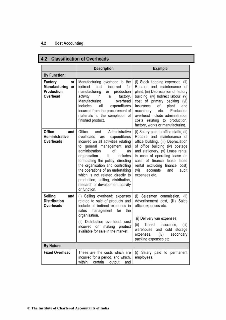
4.2 Cost Accounting
4.2 Classification of Overheads
Description Example
By Function:
Factory or Manufacturing or Production Overhead
Manufacturing overhead is the indirect cost incurred for manufacturing or production activity in a factory. Manufacturing overhead includes all expenditures incurred from the procurement of materials to the completion of finished product.
(i) Stock keeping expenses, (ii) Repairs and maintenance of plant, (iii) Depreciation of factory building, (iv) Indirect labour, (v) cost of primary packing (vi) Insurance of plant and machinery etc. Production overhead include administration costs relating to production, factory, works or manufacturing.
Office and Administrative Overheads
Office and Administrative overheads are expenditures incurred on all activities relating to general management and administration of an organisation. It includes formulating the policy, directing the organisation and controlling the operations of an undertaking which is not related directly to production, selling, distribution, research or development activity or function.
(i) Salary paid to office staffs, (ii) Repairs and maintenance of office building, (iii) Depreciation of office building (iv) postage and stationery, (v) Lease rental in case of operating lease (in case of finance lease lease rental excluding finance cost) (vi) accounts and audit expenses etc.
Selling and Distribution Overheads
(i) Selling overhead: expenses related to sale of products and include all indirect expenses in sales management for the organisation.
(ii) Distribution overhead: cost incurred on making product available for sale in the market.
(i) Salesmen commission, (ii) Advertisement cost, (iii) Sales office expenses etc.
(i) Delivery van expenses,
(ii) Transit insurance, (iii) warehouse and cold storage expenses, (iv) secondary packing expenses etc.
By Nature
Fixed Overhead These are the costs which are incurred for a period, and which, within certain output and
(i) Salary paid to permanent employees,
© The Institute of Chartered Accountants of India

Overheads 4.3
turnover limits, tend to be unaffected by fluctuations in the levels of activity (output or turnover). They do not tend to increase or decrease with the changes in output.
(ii) Depreciation of building and plant and equipment, (iii) Interest on capital, (iv) Insurance
Variable Overhead
These costs tend to vary with the volume of activity. Any increase in the activity results in an increase in the variable cost and vice-versa.
(i) Indirect materials, (ii) Power and fuel, (iii) lubricants, (iv) tools and spares etc.
Semi-Variable Overheads
These costs contain both fixed and variable components and are thus partly affected by fluctuations in the level of activity.
(i) Electricity cost, (ii) water cost, (iii) telephone and internet expenses etc.
By Element
Indirect materials Materials which do not normally form part of the finished product (cost object) are known as indirect materials.
(i) Stores used for maintaining machines and buildings (lubricants, cotton waste, bricks etc.)
(ii) Stores used by service departments like power house, boiler house, canteen etc.
Indirect labour Labour costs which cannot be allocated but can be apportioned to or absorbed by cost units or cost centres is known as indirect labour.
(i) Salary paid to foreman and supervisor
(ii) Salary paid to administration staff etc.
Indirect expenses Expenses other than direct expenses are known as indirect expenses, that cannot be directly, conveniently and wholly allocated to cost centres.
(i) Rates & taxes, (ii) insurance, (iii) depreciation, (iv) advertisement expenses etc.
Controllability
Controllable costs
These are those costs which can be controlled by the implementation of appropriate managerial influence and proper
(i) Materials cost, (ii) wages and salary, (iii) power and fuel etc.
© The Institute of Chartered Accountants of India
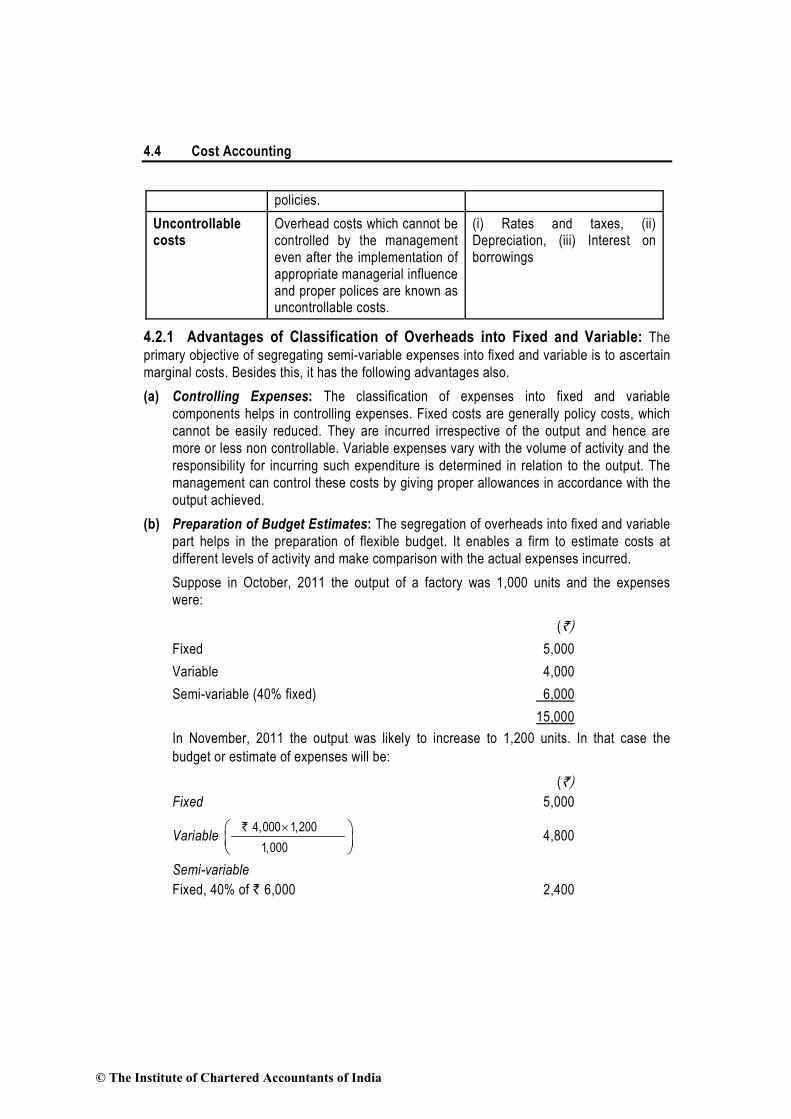
4.4 Cost Accounting
policies.
Uncontrollable costs
Overhead costs which cannot be controlled by the management even after the implementation of appropriate managerial influence and proper polices are known as uncontrollable costs.
(i) Rates and taxes, (ii) Depreciation, (iii) Interest on borrowings
4.2.1 Advantages of Classification of Overheads into Fixed and Variable: The
primary objective of segregating semi-variable expenses into fixed and variable is to ascertain
marginal costs. Besides this, it has the following advantages also.
(a) Controlling Expenses: The classification of expenses into fixed and variable
components helps in controlling expenses. Fixed costs are generally policy costs, which
cannot be easily reduced. They are incurred irrespective of the output and hence are
more or less non controllable. Variable expenses vary with the volume of activity and the
responsibility for incurring such expenditure is determined in relation to the output. The
management can control these costs by giving proper allowances in accordance with the
output achieved.
(b) Preparation of Budget Estimates: The segregation of overheads into fixed and variable
part helps in the preparation of flexible budget. It enables a firm to estimate costs at
different levels of activity and make comparison with the actual expenses incurred.
Suppose in October, 2011 the output of a factory was 1,000 units and the expenses
were:
(`)
Fixed 5,000
Variable 4,000
Semi-variable (40% fixed) 6,000
15,000
In November, 2011 the output was likely to increase to 1,200 units. In that case the
budget or estimate of expenses will be:
(`)
Fixed 5,000
Variable 4,000 1,200
1,000
×
R` units
units 4,800
Semi-variable
Fixed, 40% of ` 6,000 2,400
© The Institute of Chartered Accountants of India

Overheads 4.5
Variable : 3,600 1,200
1,000
×
Rs` units
units 4,320
16,520
It would be a mistake to think that with the output going up from 1,000 units to 1,200
units the expenses would increase proportionately to `18,000. This would be wrong
budgeting.
(c) Decision Making: The segregation of semi variable cost between fixed and variable
overhead also helps the management to take many important decisions. For example,
decisions regarding the price to be charged during depression or recession or for export
market. Likewise, decisions on make or buy, shut down or continue, etc., are also taken
after separating fixed costs from variable costs.
In fact, when any change is contemplated, say, increase or decrease in production, change in
the process of manufacture or distribution, it is necessary to know the total effect on cost (or
revenue) and that would be impossible without a correct segregation of fixed and variable
costs. The technique of marginal costing, cost volume profit relationship and break-even
analysis are all based on such segregation.
4.3 Accounting and Control of Manufacturing Overheads
We have already seen that overheads are by nature those costs which cannot be directly
related to a product or to any other cost unit. Yet for working out the total cost of a product or
a unit of service, the overheads must be included. Thus we have to find out a way by which
the overheads can be distributed over the various units of production.
One method of working out the distribution of overheads over the various products could be to
ascertain the amount of actual overheads and distribute them over the products. This
however, creates a problem since the actual amount of overheads can be known only after the
financial accounts are closed. If we wait that long, the cost sheets lose their main advantages
and utility to the management. All the decisions for which cost sheets are prepared are
immediate decisions and cannot be postponed till the actual overheads are known. Therefore,
some method has to be found by which overheads can be included in the cost of the products,
as soon as prime cost, the cost of raw materials, labour and other direct expenses, is
ascertained.
One method is to work out pre-determined rates for absorbing overheads. These rates are
worked out before an accounting period begins by estimating the amount of overheads and
the level of activity in the ensuing period. Thus, as soon as the prime cost of a product or a job
is available, the various overheads are charged by these rates. Of course, this implies that the
overheads are charged on an estimated basis. Later, when the actual overheads are known,
the difference between the overheads charged to the products and actual overheads is worked
out and adjusted.
© The Institute of Chartered Accountants of India

4.6 Cost Accounting
Manufacturing Overheads: Generally manufacturing overheads form a substantial portion of
the total overheads. It is important, that such overheads should be properly absorbed over the
cost of production. The following procedure may be adopted in this regard. The steps given
below shows how factory overhead rates are estimated and overheads absorbed on that basis
and the last one shows how actual are compared with the absorbed amount.
(Students should carefully note the distinction between the various terms used).
1. Estimation and collection of manufacturing overheads: The first stage is to estimate
the amount of overheads, keeping in view the past figures and adjusting them for known future
changes. The sources available for the collection of factory overheads may include (a)
Invoices, (b) Stores requisition, (c) Wage analysis book (d) Journal entries. etc.
2. Assignment of Manufacturing Overheads: The guiding principle for assignment of
manufacturing overheads to a cost object is the traceability of the overheads in an
economically feasible manner.
Assignment of the manufacturing overhead is done on the basis of either of the following
two principles:
(i) Cause and Effect: Cause is the process or operation or activity and effect is the
incurrence of cost.
(ii) Benefit received: Manufacturing overheads are to be apportioned to various cost
objects in proportion to the benefits received by them.
(a) Cost Allocation: The term ‘allocation’ refers to the direct assignment of cost to a cost
object which can be traced directly. It implies relating overheads directly to the various
departments. The estimated amount of various items of manufacturing overheads should be
allocated to various cost centres or departments. For example- if a separate power meter has
been installed for a department, the entire power cost ascertained from the meter is allocated
to that department. The salary of the works manager cannot be directly allocated to any one
department since he looks after the whole factory. It is, therefore, obvious that many overhead
items will remain unallocated after this step.
(b) Cost Apportionment: There are some items of estimated overheads (like the salary of
the works manager) which cannot be directly allocated to the various departments and cost
centres. Such unallocable expenses are to be spread over the various departments or cost
centres on the basis of two principles. This is called apportionment. Thus apportionment
implies “the allotment of proportions of items of cost to cost centres or departments”. After this
stage, all the overhead costs would have been either allocated to or apportioned over the
various departments.
(c) Re-apportionment: Upto the last stage all overheads are allocated and apportioned to
all the departments- both production and service departments. Service departments are those
departments which do not directly take part in the production of goods or providing services.
Such departments provide auxiliary services across the entity and renders services to other
© The Institute of Chartered Accountants of India

Overheads 4.7
cost centres and in some cases to outside parties. Examples of such departments are
engineering, quality control and assurance, laboratory, canteen, stores, time office, dispensary
etc. The overheads of these departments are to be shared by the production departments
since service departments operate primarily for the purpose of providing services to
production departments. The process of assigning service department overheads to
production departments is called reassignment or re-apportionment. At this stage, all the
factory overheads are collected under production departments.
3. Absorption: After completing the distribution as stated above the overheads charged to
department are to be recovered from the output produced in respective departments. This
process of recovering overheads of a department or any other cost center from its output is
called recovery or absorption.
Absorption of manufacturing overheads shall be as follows:
(i) Variable Manufacturing overheads: The variable manufacturing overheads shall be
absorbed on the basis of actual production.
(ii) Fixed Manufacturing overheads: The fixed manufacturing overhead shall be
absorbed on the basis of normal capacity.
The overhead expenses can be absorbed by estimating the overhead (as assigned above)
and then working out an absorption rate. When overheads are estimated, their absorption is
carried out by adopting a pre-determined overhead absorption rate. This rate can be
calculated by using any one method as discussed in this chapter at the end.
As the actual accounting period begins, each unit of production automatically absorbs a
certain amount of factory overheads through pre-determined rates. During the year a certain
amount will be absorbed over the various products. This is known as the total amount of
absorbed overheads.
4. Treatment of over and under absorption of overheads: After the year end the total
amount of actual factory overheads is known. There is bound to be some difference between
the actual amount of overheads and the absorbed amount of overheads. So the overheads are
generally either under-absorbed or over-absorbed. The difference has to be adjusted keeping
in view of such differences and the reasons therefore.
Students will thus see that the whole discussion as above is meant to serve the following two
purposes:
(a) to charge various products and services with an equitable portion of the total amount of
factory overheads ; and
(b) to charge factory overheads immediately as the product or the job is completed without
waiting for the figures of actual factory overheads.
© The Institute of Chartered Accountants of India

4.8 Cost Accounting
4.4 Steps for the Distribution of Overheads
The various steps for the distribution of overheads have been discussed in detail as below:
4.4.1 Estimation and Collection of Manufacturing Overheads: The amount of factory
overheads is required to be estimated. The estimation is usually done with reference to past
data adjusted for known future changes. The overhead expenses are usually collected through
a system of standing orders.
Standing Orders: In every manufacturing business, expenses are incurred on direct materials
and direct labour in respect of several jobs or other units of production, manufacture of which
is undertaken. The incurring of these expenses is authorised by production orders or work
orders. The work order numbers are not ordinarily fixed or permanent. They are generally
allotted in a serial order according to the number of manufacturing jobs undertaken by the
business. In addition, indirect expenses are incurred in connection with the rendering of
services to the production departments, or to the manufacturing process. The term “Standing
Order” denotes sanction for indirect expenses under various heads of expenditure.
In large factories, usually the classification of indirect expenditures is combined with a system
of Standing Orders (sometimes also referred as Service “Orders”). It is a system under which
a number is allotted to each item of expense for the purpose of identification, and the same is
continued from year to year. All the indirect expenditure in such a case, is charged to one or
the other of the Standing Orders and periodical summaries, giving total of each Standing
Order, are prepared for comparison with budgets, as well as for apportioning them among the
various departments. The extent of such analysis and the nomenclature adopted are settled
by the management according to the needs of the industry.
4.4.2 Allocation of Overheads over various Departments or Departmentalisation of Overheads: Most of the manufacturing processes functionally are different and are
performed by different departments in the factory. Where such a division of functions had been
made, some of the departments should be engaged in actual production of goods, and others
in providing services ancillary thereto. At this stage, the factory overheads which can be
directly related to the various production or service departments are allocated in this manner.
It may, sometime, become necessary to sub-divide a manufacturing organisation into several
cost centres, so that a closer distribution of expenses and a more detailed control is
practicable.
It is thus obvious that the principal object of setting up cost centres is to collect data, in
respect of similar activities more conveniently. This avoids a great deal of cost analysis. When
costs are collected by setting up cost centres, several items can be ascertained definitely and
the element of estimation is reduced considerably. For instance, the allowance of the normal
idle time or the amount to be spent on consumable stores, etc. There are two main types of
cost centres - machine or personal - depending on whether the process of manufacture is
carried on at a centre by man or machine. For the convenience of recording of expenditure,
© The Institute of Chartered Accountants of India

Overheads 4.9
cost centres are sometimes allotted a code number.
Advantages of Departmentalisation: The collection of overheads department wise gives rise to
the following advantages:
(a) Better Estimation of Expenses: Some expenses which relate to the departments will be
estimated almost on an exact basis and, to that extent, the accuracy of estimation of
overheads will be higher.
(b) Better Control: For the purpose of controlling expenses in a department, it is obviously
necessary that the figures in relation to each department should be separately available.
It is one of the main principles of control that one should know for each activity how
much should have been spent and how much is actually spent. If information about
expenses is available only for factory as a whole, it will not be possible to know which
department has been over spending.
(c) Ascertainment of Cost for each department: From the point of view of ascertaining the
cost of each job, the expenses incurred in the departments through which the job or the
product has passed should be known. It is only then that the cost of the job or the
product can be charged with the appropriate share of indirect expenses. It is not
necessary that a job must pass through all the departments or that the work required in
each department should be the same for all jobs. It is, therefore, necessary that only
appropriate charge in respect of the work done in the department is made. This can be
done only if overheads for each department are known separately.
(d) Suitable Method of Costing: A suitable method of costing can be followed differently for
each department e.g., batch costing when a part is manufactured, but single or output
costing when the product is assembled.
4.4.3 Apportioning overhead expenses over various departments: After the
allocable overheads are related to the departments, expenses incurred for several
departments have to be apportioned over each department, e.g. rent, power, lighting,
insurance and depreciation. For distributing these overheads over different departments
benefiting thereby, it is necessary at first to determine the proportion of benefit received by
each department and then distribute the total expenditure proportionately on that basis. But
the same basis of apportionment cannot be followed for different items of overheads since the
benefit of service to a department in each case has to be measured differently. Some of the
bases that may be adopted for the apportionment of expenses are stated below:
Overhead Cost Bases of Apportionment
1. (i) Rent and other building expenses
(ii) Lighting and heating (conditioning)
(iii) Fire precaution service
(iv) Air- conditioning
Floor area, or volume of department
2. (i) Perquisites Number of workers
© The Institute of Chartered Accountants of India

4.10 Cost Accounting
(ii) Labour welfare expenses
(iii) Time keeping
(iv) Personnel office
(v) Supervision
3. (i) Compensation to workers
(ii) Holiday pay
(iii) ESI and PF contribution
(iv) Perquisites
Direct wages
4. General overhead Direct labour hour, or Direct wages, or Machine hours.
5. (i) Depreciation of plant and machinery
(ii) Repairs and maintenance of plant and machinery
(iii) Insurance of stock
Capital values
6. (i) Power/steam consumption
(ii) Internal transport
(iii) Managerial salaries
Technical estimates
7. Lighting expenses (light) No. of light points, or Area or Metered units
8. Electric power (machine operation) Horse power of machines, or Number of machine hour, or value of machines or units consumed.
9. (i) Material handling
(ii) Stores overhead
Weight of materials, or volume of materials, or value of materials or unit of materials.
Some other basis of apportioning overhead costs: We have considered already that the
benefit received by the department generally is the principal criterion on which the costs of
service departments or common expenses are apportioned. But other bases of
apportionments which may be used are mentioned below:
(a) Analysis or survey of existing conditions.
(b) Ability to pay.
(c) Efficiency or incentive.
A single concern may have only one criterion under consideration predominantly or may use
all (including the service or benefit criterion) for different phases of its activity.
Analysis or Survey of existing conditions : At times it may not be possible to determine the
advantage of an item of expenses without undertaking an analysis of expenditure. For
example, lighting expenses can be distributed over departments only on the basis of the
number of light points fixed in each department.
© The Institute of Chartered Accountants of India

Overheads 4.11
Ability to pay: It is a principle of taxation which has been applied in cost accounting as well
for distributing the expenditure on the basis of income of the paying department, on a pro-
portionate basis. For example, if a company is selling three different products in a territory, it
may decide to distribute the expenses of the sales organisation to the amount of sales of
different articles in these territories. This basis, though simple to apply, may be inequitable
since the expenditure charged to an article may have no relation to the actual effort involved in
selling it. Easy selling lines thus may have to bear the largest proportion of expenses while, on
the other hand, these should bear the lowest charge.
Efficiency or Incentives: Under this method, the distribution of overheads is made on the
basis of pre-determined levels of production or sales. When distribution of overhead cost is
made on this basis and if the level of production exceeds the pre-determined level of
production the incidence of overhead cost gets reduced and the total cost per unit of
production or of sales, lowered. The opposite is the effect if the assumed levels are not
reached.
Thus the department whose sales are increasing is able to show a greater profit and thereby is
able to earn greater goodwill and appreciation of the management than it would have if the
distribution of overheads was made otherwise.
Difference between Allocation and Apportionment
The difference between the allocation and apportionment is important to understand because
the purpose of these two methods is the identification of the items of cost to cost units or
centers. However, the main difference between the above methods is given below.
(1) Allocation deals with the whole items of cost, which are identifiable with any one
department. For example, indirect wages of three departments are separately obtained
and hence each department will be charged by the respective amount of wages
individually.
On the other hand apportionment deals with the proportions of an item of cost for
example; the cost of the benefit of a service department will be divided between those
departments which has availed those benefits.
(2) Allocation is a direct process of charging expenses to different cost centres whereas
apportionment is an indirect process because there is a need for the identification of the
appropriate portion of an expense to be borne by the different departments benefited.
(3) The allocation or apportionment of an expense is not dependent on its nature, but the
relationship between the expense and the cost centre decides that whether it is to be
allocated or apportioned.
(4) Allocation is a much wider term than apportionment.
4.4.4 Re-apportioning service department overheads over production department: The re-apportionment of the service department cost to the production
© The Institute of Chartered Accountants of India

4.12 Cost Accounting
department is known as secondary distribution. The suggestive bases that may be adopted for
re-apportionment are given below:
Cost of the Service Departments: Basis
1. Maintenance and Repair shop
2. Planning and progress
3 Tool room
×
Direct labour hours, Machine hours,
Direct labour wages, Asset value
Hours worked.
4. Canteen and Welfare
5. Hospital and Dispensary
6. Personnel Department
No. of direct workers
No. of employees etc.
7. Time-keeping No. of card punched, No. of employees
8. Computer Section Computer hours, Specific allocation to
departments
9. Power House (electric lighting cost) Floor area, Cubic content, No. of electric
Points, Wattage.
10. Power House (electric power cost) Horse power, Kwh, Horse power × Machine
hours, Kwh × Machine hours
11. Stores Department No. of requisitions, Weight or value of
Materials issued.
12. Transport Department Crane hours, Truck hours, Truck mileage,
Truck tonnage, Truck ton- hours, Tonnage
handled. No. of packages of Standard size
13. Fire Protection Capital values
14. Inspection Inspection hours
Notes:
(1) Repairs included in repairs shop cost, building maintenance cost included in
maintenance shop cost etc. should be apportioned on the basis of capital values.
(2) Economy, practicability, equitability and reliability are the matters of consideration for
selection of the base.
Methods for Re-apportionment: The re-apportionment of service department expenses over
the production departments may be carried out by using any one of the following methods:
(i) Direct re-distribution method.
(ii) Step method of secondary distribution or non-reciprocal method.
(iii) Reciprocal Service method.
© The Institute of Chartered Accountants of India

Overheads 4.13
(i) Direct Re-distribution Method: Service department costs under this method are
apportioned over the production departments only, ignoring the services rendered by one
service department to the other. To understand the applications of this method go through the
illustration which follows.
Illustration 1: (Re-apportionment of costs under Direct re-distribution method)
XL Ltd., has three production departments and four service departments. The expenses for
these departments as per Primary Distribution Summary are as follows :
Production Departments : (`) (`)
A 30,000
B 26,000
C 24,000 80,000
Service Departments : (`) (`)
Stores 4,000
Time-keeping and Accounts 3,000
Power 1,600
Canteen 1,000 9,600
The following information is also available in respect of the production departments:
Dept. A Dept. B Dept. C
Horse power of Machine 300 300 200
Number of workers 20 15 15
Value of stores requisition in (` ) 2,500 1,500 1,000
Apportion the costs of service departments over the production departments.
Solution
Secondary Overhead Distribution Statement
Item of cost Basis of Total Production Depts
(as per primary apportionment
distribution A B C
summary) (`) (`) (`) (`)
Cost as per primary 80,000 30,000 26,000 24,000
distribution summary
Stores Value of
(5:3:2) Store requisition 4,000 2,000 1,200 800
© The Institute of Chartered Accountants of India
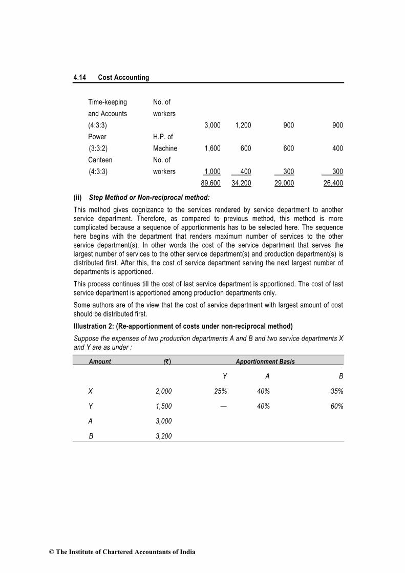
4.14 Cost Accounting
Time-keeping No. of
and Accounts workers
(4:3:3) 3,000 1,200 900 900
Power H.P. of
(3:3:2) Machine 1,600 600 600 400
Canteen No. of
(4:3:3) workers 1,000 400 300 300
89,600 34,200 29,000 26,400
(ii) Step Method or Non-reciprocal method:
This method gives cognizance to the services rendered by service department to another
service department. Therefore, as compared to previous method, this method is more
complicated because a sequence of apportionments has to be selected here. The sequence
here begins with the department that renders maximum number of services to the other
service department(s). In other words the cost of the service department that serves the
largest number of services to the other service department(s) and production department(s) is
distributed first. After this, the cost of service department serving the next largest number of
departments is apportioned.
This process continues till the cost of last service department is apportioned. The cost of last
service department is apportioned among production departments only.
Some authors are of the view that the cost of service department with largest amount of cost
should be distributed first.
Illustration 2: (Re-apportionment of costs under non-reciprocal method)
Suppose the expenses of two production departments A and B and two service departments X
and Y are as under :
Amount (`) Apportionment Basis
Y A B
X 2,000 25% 40% 35%
Y 1,500 — 40% 60%
A 3,000
B 3,200
© The Institute of Chartered Accountants of India

Overheads 4.15
Solution
Summary of Overhead Distribution
Departments X Y A B
(`) (`) (`) (`)
Amount as given above 2,000 1,500 3,000 3,200
Expenses of X Dept.
apportioned over Y,A and
B Dept. in the ratio (5:8:7) —2,000 500 800 700
Expenses of Y Dept.
apportioned over A and
B Dept. in the ratio (2:3) - —2,000 800 1,200
Total Nil Nil 4,600 5,100
(iii) Reciprocal Service Method: This method recognises the fact that where there are two
or more service departments they may render services to each other and, therefore, these
inter-departmental services are to be given due weight while re-distributing the expenses of
the service departments.
The methods available for dealing with reciprocal services are:
(a) Simultaneous equation method;
(b) Trial and error method;
(c) Repeated distribution method.
(a) Simultaneous Equation Method: According to this method firstly, the costs of service
departments are ascertained. These costs are then re-distributed to production departments
on the basis of given percentages. (Refer to the following illustration to understand the
method)
Illustration 3: (Re-apportionment of costs under Simultaneous equation method)
Service departments’ expenses
(`) Boiler House 3,000
Pump Room 600
3,600
© The Institute of Chartered Accountants of India

4.16 Cost Accounting
The allocation is :
Production Departments Boiler House Pump Room
A B
Boiler House 60% 35% – 5%
Pump Room 10% 40% 50% –
Solution
The total expenses of the two service departments will be determined as follows:
Let B stand for Boiler House expenses and P for Pump Room expenses.
Then
B = 3,000 + 1/2 P
P = 600 + 1/20 B
Substituting the value of B,
P = 600 + 1/20 (3,000 + 1/2 P)
= 600 + 150 + 1/40 P
= 750 + 1/40 P
40 P = 30,000 + P
39 P = 30,000
P = ` 769 (approx.)
The total of expenses of the Pump Room are ` 769 and that of the Boiler House is ` 3,385
i.e., ` 3,000 + 1/2 × ` 769.
The expenses will be allocated to the production departments as under:
Production departments: A B
(`) (`)
Boiler House (60% and 35% of ` 3,385) 2,031 1,185
Pump Room (10% and 40% of ` 769) 77 307
Total 2,108 1,492
The total of expenses apportioned to A and B is ` 3,600.
(b) Trial and Error Method: According to this method the cost of one service cost centre is
apportioned to another service cost centre. The cost of another service centre plus the share
received from the first cost centre is again apportioned to the first cost centre. This process is
repeated till the amount to be apportioned becomes negligible, that means repeated
distribution method is followed to the extent of service departments only. All apportioned
amounts for each service cost centre are added to get the total apportioned cost. These total
© The Institute of Chartered Accountants of India

Overheads 4.17
service cost centre costs are redistributed to the production departments. Trial and error
method and Simultaneous equation method gives the same result. (Refer to the following
illustration to understand this method.)
Illustration 4: (Re-apportionment of costs under Trial and error method)
Sanz Ltd., is a manufacturing company having three production departments, ‘A’, ‘B’ and ‘C’
and two service departments ‘X’ and ‘Y’. The following is the budget for December 2013:
Total A B C X Y
(`) (`) (`) (`) (`) (`)
Direct material 1,000 2,000 4,000 2,000 1,000
Direct wages 5,000 2,000 8,000 1,000 2,000
Factory rent 4,000
Power 2,500
Depreciation 1,000
Other overheads 9,000
Additional information:
Area (Sq. ft.) 500 250 500 250 500
Capital value of assets (` lacs) 20 40 20 10 10
Machine hours 1,000 2,000 4,000 1,000 1,000
Horse power of machines 50 40 20 15 25
A technical assessment of the apportionment of expenses of service departments is as under:
A B C X Y
Service Dept. ‘X’ (%) 45 15 30 – 10
Service Dept. ‘Y’ (%) 60 35 – 5 –
Required:
(i) A statement showing distribution of overheads to various departments.
(ii) A statement showing re-distribution of service departments expenses to production
departments using Trial and error method.
Solution
(i) Overhead Distribution Summary
Basis Total A B C X Y
(`) (`) (`) (`) (`) (`)
Direct materials Direct – – – – 2,000 1,000
Direct wages Direct – – – – 1,000 2,000
© The Institute of Chartered Accountants of India

4.18 Cost Accounting
Factory rent Area 4,000 1,000 500 1,000 500 1,000
Power H.P. × M/c Hrs. 2,500 500 800 800 150 250
Depreciation Cap. value 1,000 200 400 200 100 100
Other overheads M/c hrs. 9,000 1,000 2,000 4,000 1,000 1,000
16,500 2,700 3,700 6,000 4,750 5,350
(ii) Redistribution of Service Department’s expenses:
Service Departments
X (`) Y (`)
Overheads as per primary distribution 4,750 5,350
(i) Apportionment of Dept-X expenses to Dept-Y
(10% of ` 4,750) --- 475
(ii) Apportionment of Dept-Y expenses to Dept-X
[5% of (` 5,350 + ` 475)] 291 ---
(i) Apportionment of Dept-X expenses to Dept-Y
(10% of ` 291) --- 29
(ii) Apportionment of Dept-Y expenses to Dept-X
(5% of ` 29) 2 ---
Total 5,043 5,854
Distribution of Service departments’ overheads to Production departments
Production Departments
A (`) B (`) C (`)
Overhead as per primary distribution 2,700 3,700 6,000
Dept- X (90% of ` 5,043) 2,269 756 1,513
Dept- Y (95% of ` 5,854) 3,513 2,049 ---
8,482 6,505 7,513
(c) Repeated Distribution Method: Under this method, service departments’ costs are
distributed to other service and production departments on agreed percentages and this
process continues to be repeated, till the figures of service departments are either exhausted
or reduced to too small a figure. (Refer to the following illustration to understand this method)
Illustration 5: (Re-apportionment of costs under Repeated distribution method)
PH Ltd., is a manufacturing company having three production departments, ‘A’, ‘B’ and ‘C’ and
two service departments ‘X’ and ‘Y’. The following is the budget for December 2011:
© The Institute of Chartered Accountants of India

Overheads 4.19
Total A B C X Y
(`) (`) (`) (`) (`) (`)
Direct material 1,000 2,000 4,000 2,000 1,000
Direct wages 5,000 2,000 8,000 1,000 2,000
Factory rent 4,000
Power 2,500
Depreciation 1,000
Other overheads 9,000
Additional information:
Area (Sq. ft.) 500 250 500 250 500
Capital value of assets (` lacs) 20 40 20 10 10
Machine hours 1,000 2,000 4,000 1,000 1,000
Horse power of machines 50 40 20 15 25
A technical assessment of the apportionment of expenses of service departments is as under:
A B C X Y
Service Dept. ‘X’ (%) 45 15 30 – 10
Service Dept. ‘Y’ (%) 60 35 – 5 –
Required:
(i) A statement showing distribution of overheads to various departments.
(ii) A statement showing re-distribution of service departments expenses to production
departments.
(iii) Machine hour rates of the production departments ‘A’, ‘B’ and ‘C’.
Solution
(i) Overhead Distribution Summary
Basis Total A B C X Y
(`) (`) (`) (`) (`) (`)
Direct materials Direct – – – – 2,000 1,000
Direct wages Direct – – – – 1,000 2,000
Factory rent Area 4,000 1,000 500 1,000 500 1,000
Power H.P. × M/c Hrs. 2,500 500 800 800 150 250
Depreciation Cap. value 1,000 200 400 200 100 100
Other overheads M/c hrs. 9,000 1,000 2,000 4,000 1,000 1,000
16,500 2,700 3,700 6,000 4,750 5,350
© The Institute of Chartered Accountants of India

4.20 Cost Accounting
(ii) Redistribution of Service Department’s expenses:
A B C X Y
(`) (`) (`) (`) (`)
Total overheads 2,700 3,700 6,000 4,750 5,350
Dept. X overhead apportioned
in the ratio (45:15:30:—:10) 2,138 712 1,425 –4,750 475
Dept. Y overhead apportioned
in the ratio (60: 35:—:5 :—) 3,495 2,039 − 291 –5,825
Dept. X overhead apportioned
in the ratio (45:15:30:—:10) 131 44 87 –291 29
Dept. Y overhead apportioned
in the ratio (60:35:—:5:—) 17 10 − 2 –29
Dept. X overhead apportioned
in the ratio (45:15:30:—:10) 1 − 1 –2 −
8,482 6,505 7,513 − −
(iii) Machine hour rate:
Machine hours 1,000 2,000 4,000
Machine hour rate (`) 8.48 3.25 1.88
(` 8,482/ 1,000 hrs) (` 6,505/ 2,000 hrs.) (` 7,513/ 4,000 hrs.)
Illustration 6: (Re-apportionment of costs under Repeated distribution method)
The ABC Company has the following account balances and distribution of direct charges on
31st March, 2011.
Total Production Depts. Service Depts.
Machine Packing Gen. Store &
Shop Plant Maintenance
Allocated Overheads: (`) (`) (`) (`) (`)
Indirect labour 14,650 4,000 3,000 2,000 5,650
Maintenance material 5,020 1,800 700 1,020 1,500
Misc. supplies 1,750 400 1,000 150 200
Superintendent’s salary 4,000 – – 4,000 –
Cost & payroll salary 10,000 – – 10,000 –
Overheads to be apportioned :
© The Institute of Chartered Accountants of India
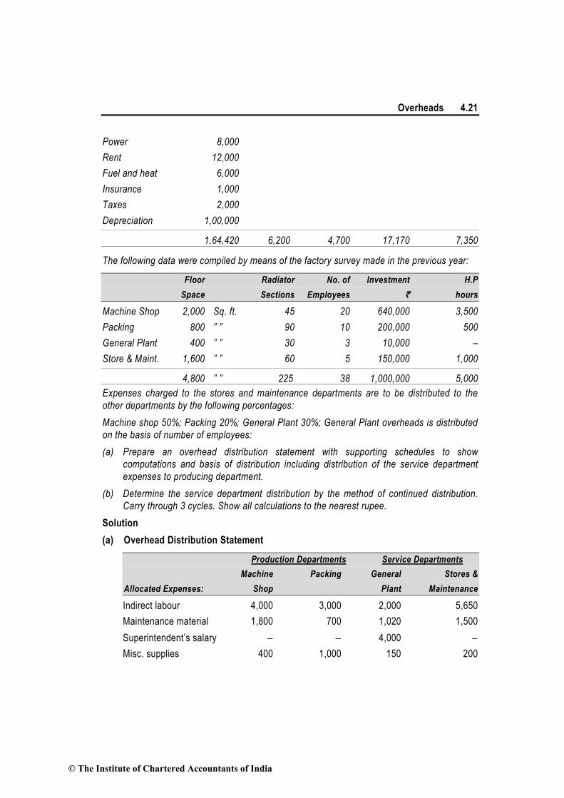
Overheads 4.21
Power 8,000
Rent 12,000
Fuel and heat 6,000
Insurance 1,000
Taxes 2,000
Depreciation 1,00,000
1,64,420 6,200 4,700 17,170 7,350
The following data were compiled by means of the factory survey made in the previous year:
Floor Radiator No. of Investment H.P
Space Sections Employees ` hours
Machine Shop 2,000 Sq. ft. 45 20 640,000 3,500
Packing 800 ” ” 90 10 200,000 500
General Plant 400 ” ” 30 3 10,000 –
Store & Maint. 1,600 ” ” 60 5 150,000 1,000
4,800 ” ” 225 38 1,000,000 5,000
Expenses charged to the stores and maintenance departments are to be distributed to the
other departments by the following percentages:
Machine shop 50%; Packing 20%; General Plant 30%; General Plant overheads is distributed
on the basis of number of employees:
(a) Prepare an overhead distribution statement with supporting schedules to show
computations and basis of distribution including distribution of the service department
expenses to producing department.
(b) Determine the service department distribution by the method of continued distribution.
Carry through 3 cycles. Show all calculations to the nearest rupee.
Solution
(a) Overhead Distribution Statement
Production Departments Service Departments
Machine Packing General Stores &
Allocated Expenses: Shop Plant Maintenance
Indirect labour 4,000 3,000 2,000 5,650
Maintenance material 1,800 700 1,020 1,500
Superintendent’s salary − − 4,000 −
Misc. supplies 400 1,000 150 200
© The Institute of Chartered Accountants of India

4.22 Cost Accounting
Cost & payroll salaries − − 10,000 −
Total 6,200 4,700 17,170 7,350
Apportioned expenses
(See schedule below) 77,720 25,800 2,830 22,650
Total 83,920 30,500 20,000 30,000
Schedule of Apportioned Expenses
Item Basis Machine Packing General Stores &
Shop Plant Maintenance
(`) (`) (`) (`)
Power Horse Power Hrs. 5,600 800 – 1,600
Rent Floor Space 5,000 2,000 1,000 4,000
Fuel & Heat Radiator Secs. 1,200 2,400 800 1,600
Insurance Investment 640 200 10 150
Taxes Investment 1,280 400 20 300
Depreciation Investment 64,000 20,000 1,000 15,000
Total 77,720 25,800 2,830 22,650
(b) Distribution of Service Department Expenses
Production Departments Service Departments
Machine Packing General Stores &
Plant Maintenance
(`) (`) (`) (`)
Total Expense [as per (a)] 83,920 30,500 20,000 30,000
Transfer from Stores &
Maintenance 15,000 6,000 9,000 –30,000
Transfer from General Plant 16,571 8,286 –29,000 4,143
Transfer from Stores &
Maintenance 2,072 829 1,242 –4,143
Transfer from General Plant 710 355 –1,242 177
Transfer from Stores &
Maintenance 88 36 53 –177
Transfer from General Plant 35 18 –53 —
Total 1,18,396 46,024 — —
© The Institute of Chartered Accountants of India
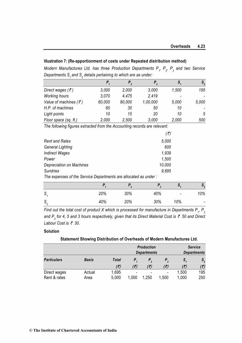
Overheads 4.23
Illustration 7: (Re-apportionment of costs under Repeated distribution method)
Modern Manufactures Ltd. has three Production Departments P1, P
2, P
3 and two Service
Departments S1
and S2 details pertaining to which are as under:
P1 P
2 P
3 S
1 S
2
Direct wages (` ) 3,000 2,000 3,000 1,500 195
Working hours 3,070 4,475 2,419 - -
Value of machines (` ) 60,000 80,000 1,00,000 5,000 5,000
H.P. of machines 60 30 50 10 -
Light points 10 15 20 10 5
Floor space (sq. ft.) 2,000 2,500 3,000 2,000 500
The following figures extracted from the Accounting records are relevant:
(`)
Rent and Rates 5,000
General Lighting 600
Indirect Wages 1,939
Power 1,500
Depreciation on Machines 10,000
Sundries 9,695
The expenses of the Service Departments are allocated as under :
P1 P
2 P
3 S
1 S
2
S1 20% 30% 40% - 10%
S2 40% 20% 30% 10% -
Find out the total cost of product X which is processed for manufacture in Departments P1, P
2
and P3 for 4, 5 and 3 hours respectively, given that its Direct Material Cost is ` 50 and Direct
Labour Cost is ` 30.
Solution
Statement Showing Distribution of Overheads of Modern Manufactures Ltd.
Production Service
Departments Departments
Particulars Basis Total P1 P
2 P
3 S
1 S
2
(`) (`) (`) (`) (`) (`)
Direct wages Actual 1,695 - - - 1,500 195
Rent & rates Area 5,000 1,000 1,250 1,500 1,000 250
© The Institute of Chartered Accountants of India

4.24 Cost Accounting
General lighting Light points 600 100 150 200 100 50
Indirect wages Direct wages 1,939 600 400 600 300 39
Power H.P. 1,500 600 300 500 100 −
Depreciation Value
of machines of machines 10,000 2,400 3,200 4,000 200 200
Sundries Direct wages 9,695 3,000 2,000 3,000 1,500 195
30,429 7,700 7,300 9,800 4,700 929
Redistribution of Service Department’s Expenses
over Production Departments
Total P1 P
2 P
3 S
1 S
2
(`) (`) (`) (`) (`) (`)
Total Overheads 30,429.00 7,700 7,300 9,800 4,700 929
Dept. S1 Overheads apportioned 4,700.00 940 1,410 1,880 –4,700 470
in the ratio: (20:30:40:—:10)
Dept. S2 overheads apportioned 1,399.00 559.60 279.80 419.70 139.90–1,399.00
in the ration :(40:20:30:10:—)
Dept. S1 overheads apportioned 139.90 27.98 41.97 55.96 –139.90 13.99
in the ratio (20:30:40:—:10)
Dept. S2 overheads apportioned 13.99 5.60 2.80 4.20 1.39 –13.99
in the ratio (40:20:30:10:—)
Dept. S1 overheads apportioned 1.39 0.28 0.42 0.56 –1.39 0.13
in the ratio (20:30:40:—:10)
Dept. S2 overheads apportioned 0.13 0.06 0.03 0.04 –0.13
in the ratio (40:20:30:10:—)
Total 9,233.52 9,035.02 12,160.46
Working hours 3,070.00 4,475.00 2,419.00
Working rate per hour 3.00 2.02 5.03
Cost of the Product ‘X’
(`) Direct material cost 50.00
Direct labour cost 30.00
Overhead cost (See working note) 37.19
117.19
© The Institute of Chartered Accountants of India

Overheads 4.25
Working Note :
Overhead cost :
(` 3 × 4 hrs.) + (` 2.02 × 5 hrs.) + (` 5.03 × 3 hrs.)
= ` 12 + ` 10.10 + ` 15.09 = ` 37.19
Illustration 8: (Re-apportionment of costs under Step Method or Step Ladder Method)
Deccan Manufacturing Ltd., have three departments which are regarded as production
departments. Service departments’ costs are distributed to these production departments
using the “Step Ladder Method” of distribution. Estimates of factory overhead costs to be
incurred by each department in the forthcoming year are as follows. Data required for
distribution is also shown against each department:
Department Factory overhead Direct labour No. of Area in
(`) hours employees sq.m.
Production:
X 1,93,000 4,000 100 3,000
Y 64,000 3,000 125 1,500
Z 83,000 4,000 85 1,500
Service:
P 45,000 1,000 10 500
Q 75,000 5,000 50 1,500
R 1,05,000 6,000 40 1,000
S 30,000 3,000 50 1,000
The overhead costs of the four service departments are distributed in the same order, viz.,
P,Q,R and S respectively on the following basis.
Department Basis
P Number of employees
Q Direct labour hours
R Area in square metres
S Direct labour hours
You are required to:
(a) Prepare a schedule showing the distribution of overhead costs of the four service
departments to the three production departments; and
(b) Calculate the overhead recovery rate per direct labour hour for each of the three
production departments.
© The Institute of Chartered Accountants of India

4.26 Cost Accounting
Solution
(a) Deccan Manufacturing Limited
Schedule Showing the Distribution of Overhead Costs among Departments
Service Production
P Q R S X Y Z
(`) (`) (`) (`) (`) (`) (`)
Overhead costs 45,000 75,000 1,05,000 30,000 1,93,000 64,000 83,000
Distribution of over-
head cost of Dept. ‘P’ (45,000) 5,000 4,000 5,000 10,000 12,500 8,500
Distribution of over-
head costs of Dept. ‘Q’ (80,000) 24,000 12,000 16,000 12,000 16,000
Distribution of over-
head cost of Dept. ‘R’ - (1,33,000) 19,000 57,000 28,500 28,500
Distribution of over-
head costs of Dept. ‘S’ - - (66,000) 24,000 18,000 24,000
Total (A) 3,00,000 1,35,000 1,60,000
(b) Direct labour hours (B) 4,000 3,000 4,000
Overhead recovery rate per hour )B(
)A( ` 75 ` 45 ` 40
4.4.5 Absorbing overheads over cost units, products, etc.: Collection of the figure of
overheads for the factory as a whole or for various departments is not enough. It is clearly
necessary to ascertain how much of the overheads is to be debited to the cost of the various
jobs, products etc. This process is called absorbing the overhead to cost units. We take up
below the various implications of this process. However, if only one uniform type of work is
done, the task is easy and under such a situation the overhead expenses to be absorbed may
be calculated by dividing actual overheads by the number of units of work done or estimated
overheads by the estimated output.
4.5 Methods of Absorbing Overheads to Various Products or Jobs
The method selected for charging overheads to products or jobs should be such as will
ensure:
(i) that the total amount charged (or recovered) in a period does not differ materially from
the actual expenses incurred in the period. and
(ii) that the amount charged to individual jobs or products is equitable. In case of factory
overhead, this means:
© The Institute of Chartered Accountants of India

Overheads 4.27
(a) that the time spent on completion of each job should be taken into consideration;
(b) that a distinction should be made between jobs done by skilled workers and those
done by unskilled workers. and
(c) that jobs done by manual labour and those done by machines should be
distinguished.
In addition, the methods should be capable of being used conveniently; and yield uniform
result from period to period as far as possible; any change that is apparent should reflect a
change in the underlying situation such as substitution of human labour by machines.
Several methods are commonly employed either individually or jointly for computing the
appropriate overhead rate. The more common of these are:
(1) Percentage of direct materials,
(2) Percentage of prime cost,
(3) Percentage of direct labour cost,
(4) Labour hour rate,
(5) Machine hour rate and
(6) Rate per unit of Output
4.5.1 Percentage of Direct material cost: Under this method, the cost of direct material
consumed is the base for calculating the amount of overhead absorbed. This overhead rate is
computed by the following formula:
Overhead rate =Total Production Overheads of a Department
×100Budgeted Direct Material cost of all products
4.5.2 Percentage of Prime cost method: This method is based on the fact that both
materials as well as labour contribute in raising factory overheads. Hence, the total of the two
i.e. Prime cost should be taken as base for absorbing the factory overhead. The overhead rate
in this method is computed by the following formals:
Overhead rate =Total Production Overheads of a Department
×100Prime Cost
Example for the above two methods:
Suppose for a given period, actual figures are estimated as follows:
`
Direct materials 2,00,000
Direct labour 1,00,000
Factory overheads 90,000
© The Institute of Chartered Accountants of India

4.28 Cost Accounting
The percentage of factory overheads to direct materials will be 45%, to prime cost 30% . If, on
a job, material cost is ` 10,000 and direct labour is ` 7,000 the cost, after absorbing factory
overhead, will be as follows :
(i) ` 17,000 + 45% ` 10,000 or ` 21,500,
(ii) ` 17,000 + 30% ` 17,000 or ` 22,100, and
One can see how, with a different method, the works cost comes out to be different. Of these
methods, the first and second are generally considered to be unsuitable on account of the
following reasons:
(i) Manufacturing overhead expenses are mostly a function of time i.e., time is the determining
factor for the incurrence and application of manufacturing overhead expenses. That they are
so would be clear if we recall that overhead expenses, specially manufacturing expenses, can
in the ultimate analysis be regarded as expenditure incurred in providing the necessary
facilities and service to workers employed in the productive process. The question of facilities
and service made available to workers naturally is dependent on the length of time during
which workers make use of the facilities. It may, therefore, be said that the job or product on
which more time has been spent would entail larger manufacturing expenses than the job
requiring less time. The factor is ignored altogether by the first method and largely by the
second method.
(ii) Overheads are neither related to the prime cost nor to direct material cost except to a very
small extent. Thus, if the percentage of material cost is used when there are two jobs
requiring the same operational time but using material having varying prices, their
manufacturing overhead cost would be different whereas this should not normally be so.
The method of absorbing overhead costs on the basis of prime cost also does not take into
consideration the time factor. The fact that the amount includes labour cost in addition to
material cost does not render the prime cost to be more suitable; infact, the results are liable
to be more misleading because of the cumulative error of using both the labour and material
cost as the basis of allocation of overhead expenses, on neither of which they are already
dependent.
(iii) Since material prices are prone to frequent and wide fluctuations, the manufacturing
overheads, if based on material cost or prime cost, also would fluctuate violently from period
to period.
(iv) The skill of the workers involved and whether machines were used or not, are ignored
when these methods are used.
Percentage of materials cost may, however, be used for the limited purpose of absorbing
material handling and store overheads.
© The Institute of Chartered Accountants of India

Overheads 4.29
4.5.3 Percentage of direct labour cost: Formula to be used under this method is-
Direct Labour Cost Percentage Rate
Overhead rate =Total Production Overheads of a Department
×100Direct Labour Cost
Advantages Disadvantages
(i) The method is simple and economical to apply.
(ii) The time factor is given recognition even if indirectly.
(iii) Total expenses recovered will not differ much from the estimated figure since total wages paid are not likely to fluctuate much.
(i) It gives rise to certain inaccuracies due to the time factor not being given full importance.
(ii) Where machinery is used to some extent in the process of manufacture, an allowance for such a factor is not made.
(iii) It does not provide for varying skills of workers
4.5.4 Labour hour rate: This method is an improvement on the percentage of direct wage
basis, as it fully recognises the significance of the element of time in the incurring and
absorption of manufacturing overhead expenses. This method is admirably suited to
operations which do not involve any large use of machinery. To calculate labour hour rate, the
amount of factory overheads is divided by the total number of direct labour hours. Suppose
factory overheads are estimated at ` 90,000 and labour hours at 1,50,000. The overhead
absorption rate will be ` 0.60. If 795 direct labour hours are spent on a job, ` 477 will be
absorbed as overhead. It can be calculated for each category of workers.
Formula to be used under this method is-
Direct Labour Hour Rate =Total Production Overheads of a Department
Direct labour Hours
4.5.5 Machine hour rate: By the machine hour rate method, manufacturing overhead
expenses are charged to production on the basis of number of hours machines are used on
jobs or work orders.
The machine hour rate is computed by the following formula:
Machine hour rate = Production overhead
No. of machine hours
There is a basic similarity between the machine hour and the direct labour hour rate method insofar
as both are based on the time factor. The choice of one or the other method is conditioned by the
actual circumstance of the individual case. In respect of departments or operations in which
machines predominate and the operators perform relatively a passive part, the machine hour rate
is more appropriate.
© The Institute of Chartered Accountants of India

4.30 Cost Accounting
In such case, the machine hour rate method alone can be depended on to correctly absorb the
manufacturing overhead expenses to different items of production. Usually, the computation is
made on the basis of the estimated expenses or the normal expenses for the coming period.
Thus the machine hour rate usually is a predetermined rate. It is desirable to work out a rate
for each individual machine; where a number of similar machines are working in a group, there
may be single rate for the whole group.
Methods of computing Machine Hour Rate: There are two methods of computing the
machine hour rate.
(i) Direct Machine hour rate: According to the first method, only the expenses directly or
immediately connected with the operation of the machine are taken into account e.g., power,
depreciation, repairs and maintenance, insurance, etc. The rate is calculated by dividing the
estimated total of these expenses for a period by the estimated number of operational hours of
the machines during the period.
(ii) Comprehensive Machine hour rate: It will be obvious, however, that in addition to the
expenses stated above there may still be other manufacturing expenses such as supervision
charges, shop cleaning and lighting, consumable stores and shop supplies, shop general
labour, rent and rates, etc. incurred for the department as a whole and, hence, not charged to
any particular machine or group of machines. In order to see that such expenses are not left
out of production costs, one should include a portion of such expenses to compute the
machine hour rate. Alternatively, the overheads not directly related to machines may be
absorbed on the basis of Productive Labour Hour Rate Method or any other suitable method.
Note: Some people even prefer to add the wages paid to the machine operator in order to get
a comprehensive rate of working a machine for one hour.
If all expenses are not allocated to machines, it will be necessary to calculate another rate for
charging the general department expenses to production. This second rate can be calculated
on the basis of direct labour hours. In effect therefore, both the machine hour and the direct
labour hour rate will be applied, though separately.
Advantages and disadvantages of Machine hour rate:
Advantages Disadvantages
(1) Where machines are the main factor of production, it is usually the best method of charging machine operating expenses to production.
(2) The under-absorption of machine overheads would indicate the extent to which the machines have been idle.
(3) It is particularly advantageous where one operator attends to several machines
(1) Additional data concerning the operation time of machines, not otherwise necessary, must be recorded and main-tained.
(2) As general department rates for all the machines in a department may be suitable, the computation of a separate machine hour rate for each machine or group of machines would mean further additional
© The Institute of Chartered Accountants of India

Overheads 4.31
(e.g. automatic screw manufacturing machine), or where several operators are engaged on the machine e.g. the belt press used in making conveyer belts.
work.
4.5.6 Rate per unit of output method: This is the simplest of all the methods. In this
method overhead rate is determined by the following formula:
Overheads rate = Amount of overhead
No. of Units
4.6 Types of Overhead Rates
The overhead rates may be of the following types:
1. Normal Rate: This rate is calculated by dividing the actual overheads by actual base. It
is also known as actual rate.
It is calculated by the following formula:
Normal overhead rate = Actual amount of overheads
Actual base
2. Pre-determined Overhead Rate: This rate is determined in advance by estimating the
amount of the overhead for the period in which it is to be used. It is computed by the following
formula:
Pre-determined rate = Budgeted amount of overhead
Budgeted base
The amount of overhead rate of expenses for absorbing them to production may be estimated
on the following three basis.
(1) The figure of the previous year or period may be adopted as the overhead rate to be
charged to production in the current year. The assumption is that the value of production
as well as overheads will remain constant or that the two will change, proportionately.
(2) The overhead rate for the year may be determined on the basis of estimated expenses
and anticipated volume of production activity.
For instance, if expenses are estimated at `10,000 and output at 4,000 units, the
overhead rate will be ` 2.50 per unit.
(3) The overhead rate for a year may be fixed on the basis of the normal volume of the
business.
3. Blanket Overhead Rate: Blanket overhead rate refers to the computation of one single
overhead rate for the whole factory. It is to be distinguished from the departmental overhead
rate which refers to a separate rate for each individual cost centre or department. The use of
© The Institute of Chartered Accountants of India
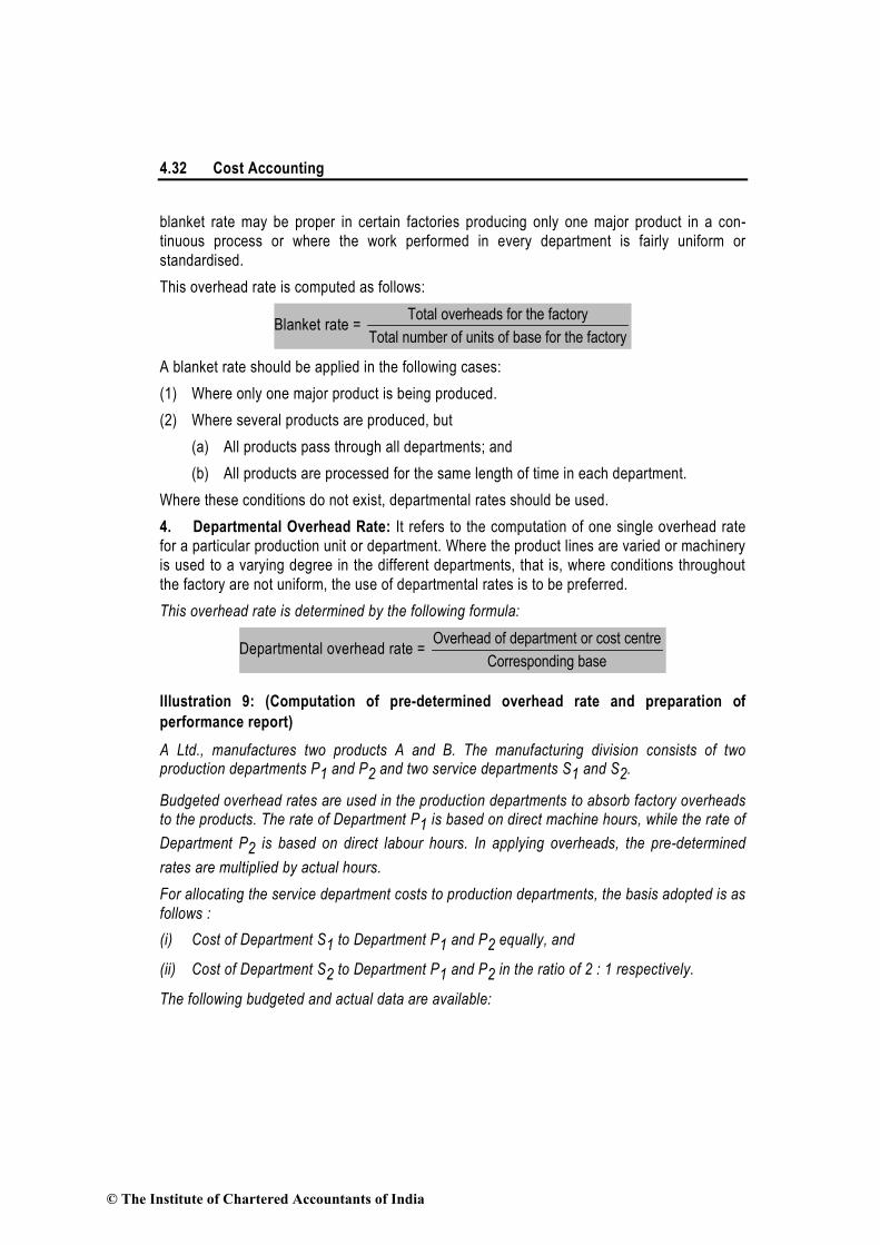
4.32 Cost Accounting
blanket rate may be proper in certain factories producing only one major product in a con-
tinuous process or where the work performed in every department is fairly uniform or
standardised.
This overhead rate is computed as follows:
Blanket rate = Total overheads for the factory
Total number of units of base for the factory
A blanket rate should be applied in the following cases:
(1) Where only one major product is being produced.
(2) Where several products are produced, but
(a) All products pass through all departments; and
(b) All products are processed for the same length of time in each department.
Where these conditions do not exist, departmental rates should be used.
4. Departmental Overhead Rate: It refers to the computation of one single overhead rate
for a particular production unit or department. Where the product lines are varied or machinery
is used to a varying degree in the different departments, that is, where conditions throughout
the factory are not uniform, the use of departmental rates is to be preferred.
This overhead rate is determined by the following formula:
Departmental overhead rate = Overhead of department or cost centre
Corresponding base
Illustration 9: (Computation of pre-determined overhead rate and preparation of
performance report)
A Ltd., manufactures two products A and B. The manufacturing division consists of two production departments P1 and P2 and two service departments S1 and S2.
Budgeted overhead rates are used in the production departments to absorb factory overheads to the products. The rate of Department P1 is based on direct machine hours, while the rate of
Department P2 is based on direct labour hours. In applying overheads, the pre-determined
rates are multiplied by actual hours.
For allocating the service department costs to production departments, the basis adopted is as
follows :
(i) Cost of Department S1 to Department P1 and P2 equally, and
(ii) Cost of Department S2 to Department P1 and P2 in the ratio of 2 : 1 respectively.
The following budgeted and actual data are available:
© The Institute of Chartered Accountants of India

Overheads 4.33
Annual profit plan data :
Factory overheads budgeted for the year:
Departments P1 25,50,000 S1 6,00,000
P2 21,75,000 S2 4,50,000
Budgeted output in units :
Product A 50,000; B 30,000.
Budgeted raw-material cost per unit :
Product A ` 120; Product B ` 150.
Budgeted time required for production per unit :
Department P1 : Product A : 1.5 machine hours
Product B : 1.0 machine hour
Department P2 : Product A : 2 Direct labour hours
Product B : 2.5 Direct labour hours
Average wage rates budgeted in Department P2 are :
Product A - ` 72 per hour and Product B – ` 75 per hour.
All materials are used in Department P1 only.
Actual data : (for the month of July, 2011)
Units actually produced : Product A : 4,000 units
Product B : 3,000 units
Actual direct machine hours worked in Department P1 :
On product A 6,100 hours, Product B 4,150 hours.
Actual direct labour hours worked in Department P2 :
on product A 8,200 hours, Product B 7,400 hours.
Costs actually incurred:
Product A Product B
` ` Raw materials 4,89,000 4,56,000
Wages 5,91,900 5,52,000
© The Institute of Chartered Accountants of India

4.34 Cost Accounting
` ` Overheads : Department P1 2,31,000 S1 60,000
P2 2,04,000 S2 48,000
You are required to :
(i) Compute the pre-determined overhead rate for each production department.
(ii) Prepare a performance report for July, 2011 that will reflect the budgeted costs and
actual costs.
Solution
(i) Computation of predetermined overhead rate for each
production department from budgeted data
Production Deptts. Service Deptts. P1 P2 S1 S2
Budgeted factory
overheads for the year in (`) 25,50,000 21,75,000 6,00,000 4,50,000
Allocation of service department
S1’s costs to production departments
P1 and P2 equally in (`) 3,00,000 3,00,000 –6,00,000 –
Allocation of service department
S2’s costs to production departments
P1 and P2 in the ratio of 2:1 in (`) 3,00,000 1,50,000 – –4,50,000
Total (`) 31,50,000 26,25,000 Nil Nil
Budgeted machine hours in department P1 1,05,000
(Refer to working note 1)
Budgeted labour hours in department P2 1,75,000
(Refer to working note 2)
Budgeted machine hour rate
(` 31,50,000/1,05,000) ` 30
Budgeted labour hour rate
(` 26,25,000/1,75,000) ` 15
© The Institute of Chartered Accountants of India

Overheads 4.35
(ii) Performance report for July, 2011
(When 4,000 and 3,000 units of products A and B respectively were actually produced)
Budgeted Actual
(`) (`)
Raw materials used in department P1
A : 4,000 units × ` 120 4,80,000 4,89,000
B : 3,000 units × ` 150 4,50,000 4,56,000
Direct labour
Cost on the basis of labour hours
worked in department P2
A : 4,000 units × 2 hrs. × ` 72 5,76,000 5,91,900
B : 3,000 units × 2.5 hrs. × ` 75 5,62,500 5,52,000
Overhead absorbed on machine hour basis in department P1
A : 4,000 units × 1.5 hrs. × ` 30 1,80,000 1,74,400*
B : 3,000 units × 1 hr. × ` 30 90,000 1,18,649
Overhead absorbed on labour hour basis in department P2
A : 4,000 units × 2 hrs. × ` 15 1,20,000 1,31,364 **
B : 3,000 units × 2.5 hrs. × ` 15 1,12,500 1,18,548
25,71,000 26,31,861
* (Refer to working note 4) ** (Refer to working note 5)
Working notes :
Product A Product B Total
1. Budgeted output 50,000 30,000
(in units) Budgeted machine hours 75,000 30,000 1,05,000
in department P1 (50,000×1.5 hrs.) (30,000×1 hr.)
Budgeted labour hours 1,00,000 75,000 1,75,000
in department P2 (50,000×2 hrs.) (30,000×2.5 hrs.)
Product A Product B Total
2. Actual output (in units) 4,000 3,000
Actual machine hours
utilised in department P1 6,100 4,150 10,250
Actual labour hours
utilised in department P2 8,200 7,400 15,600
© The Institute of Chartered Accountants of India

4.36 Cost Accounting
3. Computation of actual overhead rates for each production department from actual data
Production Deptts. Service Deptts. P1 P2 S1 S2
Actual factory overheads for the
month of July, 2011 in (` ) 2,31,000 2,04,000 60,000 48,000
Allocation of service department
S1’s costs in (`) over production
departments P1 and P2 equally 30,000 30,000 –60,000 −
Allocation of service department
S2’s costs in (`) over production
departments P1 and P2 in the
ratio 2 : 1 32,000 16,000 − –48,000
Total (`) 2,93,000 2,50,000 Nil Nil
Actual machine hours
in department P1 10,250 − − −
(Refer to working note 2)
Actual labour hours
in department P2 − 15,600 − −
(Refer to working note 2)
Machine hour rate ` 28.59 − − −
(` 2,93,000/10,250)
Labour hour/rate − ` 16.02 − −
(` 2,50,000/15,600)
4. Actual overheads absorbed (based on machine hours)
A : 6,100 hrs × ` 28.59 = ` 1,74,400
B : 4,150 hrs × ` 28.59 = ` 1,18,649
5. Actual overheads absorbed (based on labour hours)
A : 8,200 hrs × ` 16.02 = ` 1,31,364
B : 7,400 hrs × ` 16.02 = ` 1,18,548
© The Institute of Chartered Accountants of India

Overheads 4.37
Illustration 10: (Calculation of machine hour rate)
A machine costing ` 10,000 is expected to run for 10 years. At the end of this period its scrap value is likely to be ` 900. Repairs during the whole life of the machine are expected to be ` 18,000 and the machine is expected to run 4,380 hours per year on the average. Its electricity consumption is 15 units per hour, the rate per unit being 5 paise. The machine occupies one-fourth of the area of the department and has two points out of a total of ten for lighting. The foreman has to devote about one sixth of his time to the machine. The monthly rent of the department is ` 300 and the lighting charges amount to ` 80 per month. The foreman is paid a monthly salary of ` 960. Find out the machine hour rate, assuming insurance is @ 1% p.a. and the expenses on oil, etc., are ` 9 per month.
Solution
Fixed expenses per month
(`)
Rent (one fourth of the total) 75.00
Lighting (one fifth of the total) 16.00
Foreman’s salary (one sixth of the total) 160.00
Sundry expenses–oil, waste etc. 9.00
Insurance (1% on the value of the machine per year) 8.33
Total constant expenses per month 268.33
Total number of hours per annum 4,380
Total number of hours per month 365
(`) (`)
Fixed expenses per hour : 268.33
365 hrs.
`
0.735
Variable expenses per hour :
Depreciation :
Cost of the machine 10,000
Less: Scrap value 900
9,100
Depreciation per annum 910
Depreciation per hour:910
4,380 hrs. 0.208
Repairs for the whole life 18,000
for one hour 18,000
4,380 10 years×`
0.411
Electricity for one hour : 15 units @ 0.05 P 0.750
Machine hour rate : 2.104
© The Institute of Chartered Accountants of India

4.38 Cost Accounting
Illustration 11: (Calculation of machine hour rate)
Gemini Enterprises undertakes three different jobs A, B and C. All of them require the use of a
special machine and also the use of a computer. The computer is hired and the hire charges work
out to ` 4,20,000 per annum. The expenses regarding the machine are estimated as follows:
(`) Rent for the quarter 17,500
Depreciation per annum 2,00,000
Indirect charges per annum 1,50,000
During the first month of operation the following details were taken from the job register:
Job
A B C
Number of hours the machine was used :
(a) Without the use of the computer 600 900 —
(b) With the use of the computer 400 600 1,000
You are required to compute the machine hour rate :
(a) For the firm as a whole for the month when the computer was used and when the
computer was not used.
(b) For the individual jobs A, B and C.
Solution
Working notes: (`)
(i) Total machine hours used 3,500
(600 + 900 + 400 + 600 + 1,000)
(ii) Total machine hours without the use of computers 1,500
(600 + 900)
(iii) Total machine hours with the use of computer 2,000
(400 + 600 + 1,000)
(iv)Total overheads of the machine per month
Rent (` 17,500 ÷ 3 months) 5,833.33
Depreciation (` 2,00,000 ÷ 12 months) 16,666.67
Indirect Charges (` 1,50,000 ÷ 12 months) 12,500.00
Total 35,000.00
(v) Computer hire charges for a month = ` 35,000
(` 4,20,000 ÷ 12 months)
© The Institute of Chartered Accountants of India

Overheads 4.39
(vi) Overheads for using machines without computer
= 35,000
3,500 hrs.
`
× 1,500 hrs. = ` 15,000
(vii) Overheads for using machines with computer
= 35,000
3,500 hrs
`
2,000 hrs. + ` 35,000 = ` 55,000
(a) Machine hour rate of Gemini Enterprises for the firm as a whole for a month.
(1) When the Computer was used: 55,000
2,000 hours
`
= ` 27.50 per hour
(2) When the computer was not used: 15,000
1,500 hrs.
`
= ` 10 per hour
(b) Machine hour rate for individual job
Rate per hr. Job A B C
(`) Hrs. (`) Hrs. (`) Hrs. (`)
Overheads
Without Computer 10.00 600 6,000 900 9,000 − −
With computer 27.50 400 11,000 600 16,500 1,000 27,500
1,000 17,000 1,500 25,500 1,000 27,500
Machine hour rate ` 17 ` 17 27.50
Illustration 12: (Computation of comprehensive machine hour rate)
A machine shop has 8 identical Drilling machines manned by 6 operators. The machine
cannot be worked without an operator wholly engaged on it. The original cost of all these
machines works out to ` 8 lakhs. These particulars are furnished for a 6 months period:
Normal available hours per month 208
Absenteeism (without pay) hours 18
Leave (with pay) hours 20
Normal idle time unavoidable-hours 10
Average rate of wages per worker for 8 hours a day. ` 20
Production bonus estimated 15% on wages
Value of power consumed ` 8,050
Supervision and indirect labour ` 3,300
Lighting and electricity ` 1,200
© The Institute of Chartered Accountants of India

4.40 Cost Accounting
These particulars are for a year
Repairs and maintenance including consumables 3% of value of machines.
Insurance ` 40,000
Depreciation 10% of original cost.
Other sundry works expenses ` 12,000
General management expenses allocated ` 54,530.
You are required to work out a comprehensive machine hour rate for the machine shop.
Solution
Computation of comprehensive machine hour rate of machine shop
(`) Operator’s wages 17,100
(Refer to working note 2)
Production bonus 2,565
(15% on wages)
Power consumed 8,050
Supervision and indirect labour 3,300
Lighting and electricity 1,200
Repairs and maintenance 12,000
Insurance 20,000
Depreciation 40,000
Sundry works expenses 6,000
General management expenses 27,265
1,37,480
Machine hour rate = Total overheads of machine shop
Hours of machines operation
= 1,37,480
5,760
`
hours (Refer to working note 1) = ` 23.87
Working notes.
1. Computation of hours, for which 6 operators are available for 6 months.
Normal available hours p.m. 208
per operator.
Less: Absenteeism hours 18
© The Institute of Chartered Accountants of India

Overheads 4.41
Less: Leave hours 20
Less: Idle time hours 10
48
Utilisable hours p.m. per operator 160
Total utilisable hours for 6 operators and for 6 months are = 160 × 6 × 6 = 5,760
hours
As machines cannot be worked without an operator wholly engaged on them
therefore, hours for which 6 operators are available for 6 months are the hours for
which machines can be used. Hence 5,760 hours represent total machine hours.
2. Computation of operator’s wages
Average rate of wages : 20
8
`
s = ` 2.50 per hour
Hours per month for which wages are paid to a worker (208 hours – 18 hours)
= 190 hours.
Total wages paid to 6 operators for 6 months
= 190 hours × 6 × 6 × ` 2.50 = ` 17,100
Illustration 13: (Ascertainment of works costs)
Job No. 198 was commenced on October 10, 2011 and completed on November 1, 2011.
Materials used were ` 600 and labour charged directly to the job was ` 400. Other information
is as follows:
Machine No. 215 used for 40 hours, the machine hour rate being ` 3.50.
Machine No. 160 used for 30 hours, the machine hour rate being ` 4.00. 6 welders worked on
the job for five days of 8 hours each : the Direct labour hour per welder is 20P.
Expenses not included for calculating the machine hour or direct labour hour rate totalled
` 2,000,total direct wages for the period being ` 20,000. Ascertain the works costs of job No.
198.
Solution (`) Materials 600.00
Direct labour 400.00
1,000.00
Factory overheads : (`)
Machine No. 215 : 40 hours @ ` 3.50 140.00
Machine No. 160 : 30 hours @ ` 4.00 120.00
© The Institute of Chartered Accountants of India

4.42 Cost Accounting
2401 hours of welders @ ` 0.20 per hr. 48.00
General2 10% of wages 40.00 348.00
Works cost 1,348.00
1. 6 welders × 5 days × 8 hours = 240 hours
2. Un apportioned expenses ` 2,000 which works out at 10% of direct wages.
4.7 Treatment of Under-absorbed and Over-absorbed Overheads in Cost Accounting
Overhead expenses are usually applied to production on the basis of pre-determined rates.
Production overheads are to be determined in advance as follows for fixing selling price, quote
tender price and to formulate budgets etc.
Pre-determined overhead rate =Estimated /Normal overheads for the period
Budgeted Number of units during the period
The actual overhead rate will rarely coincide with the pre-determined overhead rate, due to
variation in pre-determined overhead rate and actual overhead rate. Such a variation may
arise due to any one of the following situations:
(i) Estimated overheads for the period under consideration may remain the same or they
coincide with actual overheads but the number of units produced during the period is
either more or less in comparison with budgeted figure. In the former case actual
overhead rate will be less and in the latter case, actual overhead rate will be more than
the pre-determined overhead rate, hence over-absorption and under-absorption will
occur respectively.
(ii) Similarly, if the number of units actually produced during the period remains the same as
budgeted figure but the actual overheads incurred are more or less than the estimated
overheads for the period, then a situation of under-absorption or over-absorption will
arise respectively.
(iii) If changes occur in different proportion both in the actual overheads and in the number of
units produced during the period, then a situation of under or over-absorption (depending
upon the situation) will arise.
(iv) If the changes in the numerator (i.e. in actual overheads) and denominator (i.e. in
number of units produced) occur uniformly (without changing the proportion between the
two) then a situation of neither under nor of over-absorption will arise.
Such over or under-absorption as arrived at under different situations may also be termed as
overhead variance. The amount of over-absorption being represented by a credit balance in
© The Institute of Chartered Accountants of India

Overheads 4.43
the account and conversely, the amount of under-absorption being a debit balance.
Treatment of such under/ over absorption of overheads can be understood with the help of the
following flow chart:
As regards the treatment of such debit or credit balances, the general view is that if the
balances are small they should be transferred to the Costing Profit and Loss Account and the
cost of individual products should not be increased or reduced as these would be representing
normal cost.
Where, however the difference is large and due to wrong estimation, it would be desirable to adjust the cost of products manufactured, as otherwise the cost figures would convey a misleading impression. Such adjustments usually take the form of supplementary rates where there is a debit balance in the overhead account and a credit in the other case.
Now, the production of any period can be identified in three forms, goods finished and sold, goods finished but held in stock (not yet sold) and semi-finished goods (work in progress). So far as the first category of goods is concerned, it is arguable that the post-mortem of the costs
Treatment of Under-absorbed and Over-absorbed of overheads in Cost Accounting
© The Institute of Chartered Accountants of India

4.44 Cost Accounting
of individual products long after they have been sold may have some academic utility but it is frequently devoid of any practical significance. Therefore, it is suggested that the total variance concerning goods finished and sold should be adjusted by transferring the amount to the Cost of Sale Account, the costs of the individual items of such goods not being affected.
As regards the variance pertaining to goods finished and held in stock (i.e. not yet sold), it would be necessary to adjust the value of the stock; similarly the value of work-in-progress should be adjusted.
However, over or under recovery of overheads due to abnormal reasons (such as abnormal over or under capacity utilisation) should be transferred to the Costing Profit and Loss Account.
Illustration 14: (Use of supplementary overhead rate of absorption)
A light engineering factory fabricates machine parts to customers. The factory commenced fabrication of 12 Nos. machine parts to customers’ specifications and the expenditure incurred on the job for the week ending 21st August, 2011 is given below:
(`) (`) Direct materials (all items) 78.00
Direct labour (manual) 20 hours @` 1.50 per hour 30.00
Machine facilities :
Machine No. I : 4 hours @ ` 4.50 18.00
Machine No. II : 6 hours @ ` 6.50 39.00 57.00
Total 165.00
Overheads @ ` 0.80 per hour on 20 manual hours 16.00
Total cost 181.00
The overhead rate of ` 0.80 per hour is based on 3,000 man hours per week; similarly, the machine hour rates are based on the normal working of Machine Nos. I and II for 40 hours out of 45 hours per week.
After the close of each week, the factory levies a supplementary rate for the recovery of full overhead expenses on the basis of actual hours worked during the week. During the week ending 21st August, 2011, the total labour hours worked was 2,400 and Machine Nos. I and II had worked for 30 hours and 32½ hours respectively.
Prepare a Cost Sheet for the job for the fabrication of 12 Nos. machine parts duly levying the
supplementary rates.
Solution
Fabrication of 12 Nos. machine parts (job No......) Date of commencement : 16 August, 2011
Date of Completion. Cost sheet for the week ending, August 21, 2011 :
(`) (`) Materials 78.00
© The Institute of Chartered Accountants of India

Overheads 4.45
Labour 20 hours @ ` 1.50 30.00
Machine facilities:
Machine No. I : 4 hours @ ` 4.50 18.00
Machine No. II : 6 hours @ ` 6.50 39.00 57.00
Overheads 20 hours @ ` 0.80 per hour 16.00
181.00
Supplementary Rates
Overheads 20 hours @ ` 0.20 per hour 4.00
Machine facilities:
Machine No. I - 4 hours @ ` 1.50 6.00
Machine No. II - 6 hours @ ` 1.50 9.00 19.00
Cost 200.00
Working notes:
Overheads budgeted : 3,000 hours @ ` 0.80 = ` 2,400
Actual hours : 2,400
Actual rate per hour ` 2,400/2,400 hours = ` 1
Supplementary charge ` 0.20 (`1 – ` 0.80) per hour
Machine facilities :
Machine No. I Machine No. II
Budgeted (40 × ` 4.50) = ` 180 (40 × ` 6.50) = ` 260
Actual number of hours 30 32½
Actual rate per hour ` 6 ` 8
Supplementary rate per hour (` 6.00 – ` 4.50) (` 8.00 – ` 6.50)
` 1.50 ` 1.50
Illustration 15: (Use of supplementary overhead rate with treatment in cost accounts)
In a factory, overheads of a particular department are recovered on the basis of ` 5 per
machine hour. The total expenses incurred and the actual machine hours for the department
for the month of August were ` 80,000 and 10,000 hours respectively. Of the amount of
` 80,000, ` 15,000 became payable due to an award of the Labour Court and ` 5,000 was in
respect of expenses of the previous year booked in the current month (August). Actual
production was 40,000 units, of which 30,000 units were sold. On analysing the reasons, it
was found that 60% of the under-absorbed overhead was due to defective planning and the
rest was attributed to normal cost increase. How would you treat the under-absorbed overhead
in the cost accounts?
© The Institute of Chartered Accountants of India

4.46 Cost Accounting
Solution
Under-absorbed overhead expenses during the month of August
(`) (`)
Total expenses incurred in the month of August : 80,000
Less: The amount paid according to labour
court award (Assumed to be non-recurring) 15,000
Expenses of previous year 5,000 20,000
Net overhead expenses incurred for the month 60,000
Overhead recovered for 10,000 hours @ ` 5 per hour 50,000
Under-absorbed overheads 10,000
Treatment of under-absorbed overhead in the Cost Accounts
It is given in the question that 40,000 units were produced out of which 30,000 units were sold.
It is also given that 60% of the under-absorbed overhead was due to defective planning and
the rest was attributed to normal cost increase.
(`)
1. 60 percent of under-absorbed overhead is due to defective planning. This being abnormal, should be debited to Profit and Loss A/c
(60% of ` 10,000) 6,000
2. Balance 40 percent of under-absorbed overhead should be distributed over, Finished Goods and Cost of Sales by supplementary rate
(40% of ` 10,000) 4,000
10,000
` 4,000 may be distributed over Finished Goods and Cost of Sales as follows :
Finished Goods *` 1,000
Cost of Sales *` 3,000
*Working notes
Under-absorbed overhead : ` 4,000
Units produced : 40,000
Rate of under-absorbed overhead recover ` 0.10 per unit
Amount of under-absorbed overheads
charged to finished goods (10,000 × ` 0.10) ` 1,000
Amount of under-absorbed overheads
charged to cost of sales : (30,000 × ` 0.10) ` 3,000
© The Institute of Chartered Accountants of India
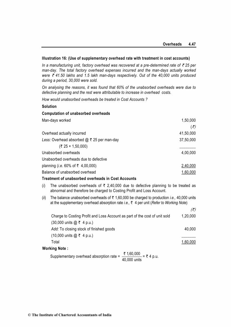
Overheads 4.47
Illustration 16: (Use of supplementary overhead rate with treatment in cost accounts)
In a manufacturing unit, factory overhead was recovered at a pre-determined rate of ` 25 per
man-day. The total factory overhead expenses incurred and the man-days actually worked
were ` 41.50 lakhs and 1.5 lakh man-days respectively. Out of the 40,000 units produced
during a period, 30,000 were sold.
On analysing the reasons, it was found that 60% of the unabsorbed overheads were due to
defective planning and the rest were attributable to increase in overhead costs.
How would unabsorbed overheads be treated in Cost Accounts ?
Solution
Computation of unabsorbed overheads
Man-days worked 1,50,000
(`)
Overhead actually incurred 41,50,000
Less: Overhead absorbed @ ` 25 per man-day 37,50,000
(` 25 × 1,50,000) ________
Unabsorbed overheads 4,00,000
Unabsorbed overheads due to defective
planning (i.e. 60% of ` 4,00,000) 2,40,000
Balance of unabsorbed overhead 1,60,000
Treatment of unabsorbed overheads in Cost Accounts
(i) The unabsorbed overheads of ` 2,40,000 due to defective planning to be treated as
abnormal and therefore be charged to Costing Profit and Loss Account.
(ii) The balance unabsorbed overheads of ` 1,60,000 be charged to production i.e., 40,000 units
at the supplementary overhead absorption rate i.e., ` 4 per unit (Refer to Working Note)
(`)
Charge to Costing Profit and Loss Account as part of the cost of unit sold 1,20,000
(30,000 units @ ` 4 p.u.)
Add: To closing stock of finished goods 40,000
(10,000 units @ ` 4 p.u.) _______
Total 1,60,000
Working Note :
Supplementary overhead absorption rate = 1,60,000
40,000 units
`
= ` 4 p.u.
© The Institute of Chartered Accountants of India

4.48 Cost Accounting
Illustration 17: (Determination of selling price under different absorption rate methods)
A factory has three production departments. The policy of the factory is to recover the production overheads of the entire factory by adopting a single blanket rate based on the percentage of total factory overheads to total factory wages. The relevant data for a month are given below:
Department Direct Direct Factory Direct Machine
Materials Wages Overheads Labour hours hours
(`) (`) (`)
Budget:
Machining 6,50,000 80,000 3,60,000 20,000 80,000 Assembly 1,70,000 3,50,000 1,40,000 1,00,000 10,000
Packing 1,00,000 70,000 1,25,000 50,000 −
Actual:
Machining 7,80,000 96,000 3,90,000 24,000 96,000 Assembly 1,36,000 2,70,000 84,000 90,000 11,000
Packing 1,20,000 90,000 1,35,000 60,000 −
The details of one of the representative jobs produced during the month are as under:
Job No. CW 7083 :
Department Direct Direct Direct Machine
Materials Wages Labour hours hours
(`) (`)
Machining 1,200 240 60 180
Assembly 600 360 120 30
Packing 300 60 40 −
The factory adds 30% on the factory cost to cover administration and selling overheads and
profit.
Required :
(i) Calculate the overhead absorption rate as per the current policy of the company and
determine the selling price of the Job No. CW 7083.
(ii) Suggest any suitable alternative method(s) of absorption of the factory overheads and
calculate the overhead recovery rates based on the method(s) so recommended by you.
(iii) Determine the selling price of Job CW 7083 based on the overhead application rates
calculated in (ii) above.
(iv) Calculate the department-wise and total under or over recovery of overheads based on
the company’s current policy and the method(s) recommended by you.
© The Institute of Chartered Accountants of India

Overheads 4.49
Solution
(i) Computation of overhead absorption rate
(as per the current policy of the company)
Department Budgeted factory overheads Budgeted direct wages
(`) (`)
Machinery 3,60,000 80,000
Assembly 1,40,000 3,50,000
Packing 1,25,000 70,000
Total 6,25,000 5,00,000
Overhead absorption rate = Budgeted factory overheads
Budgeted direct wages
× 100
= `
`
6,25,000
5,00,000× 100 = 125% of Direct wages
Selling Price of the Job No. CW-7083
(`) Direct materials (` 1,200 + ` 600 + ` 300) 2,100.00
Direct wages (` 240 + ` 360 + ` 60) 660.00
Overheads (125% × ` 660) 825.00
Total factory cost 3,585.00
Add: Mark-up (30% × ` 3,585) 1,075.50
Selling price 4,660.50
(ii) Methods available for absorbing factory overheads and their overhead recovery
rates in different departments
1. Machining Department
In the machining department, the use of machine time is the predominant factor of
production. Hence machine hour rate should be used to recover overheads in this
department. The overhead recovery rate based on machine hours has been
calculated as under:—
Machine hour rate = Budgeted factory overheads
Budgeted machine hours
=`
3,60,000
80,000 hours = ` 4.50 per hour
© The Institute of Chartered Accountants of India

4.50 Cost Accounting
2. Assembly Department
In this department direct labour hours is the main factor of production. Hence direct
labour hour rate method should be used to recover overheads in this department.
The overheads recovery rate in this case is:
Direct labour hour rate =Budgeted factory overheads
Budgeted direct labour hours
=`
1,40,000
1,00,000 hours = ` 1.40 per hour
3. Packing Department
Labour is the most important factor of production in this department. Hence direct
labour hour rate method should be used to recover overheads in this department.
The overhead recovery rate in this case comes to:
Budgeted factory overhead
Direct labour hour rate = Budgeted factory overheads
Direct labour hours
= `
1,25,000
50,000 hours = ` 2.50 per hour
(iii) Selling Price of Job CW-7083 [based on the overhead application rates calculated
in (ii) above]
(` )
Direct materials 2,100.00
Direct wages 660.00
Overheads (Refer to Working note) 1,078.00
Factory cost 3,838.00
Add: Mark up (30% of ` 3,838) 1,151.40
Selling price 4,989.40
Working note:
Overhead Summary Statement
Dept. Basis Hours Rate Overheads
(`) (`)
Machining Machine hour 180 4.50 810
Assembly Direct labour hour 120 1.40 168
© The Institute of Chartered Accountants of India

Overheads 4.51
Packing Direct labour hour 40 2.50 100
Total 1,078
(iv) Department-wise statement of total under or over recovery of overheads
(a) Under current policy
Departments
Machining Assembly Packing Total
(`) (`) (`) (`)
Direct wages (Actual) 96,000 2,70,000 90,000
Overheads recovered @
125% of Direct wages: (A) 1,20,000 3,37,500 1,12,500 5,70,000
Actual overheads: (B) 3,90,000 84,000 1,35,000 6,09,000
(Under)/Over recovery of
overheads : (A—B) (2,70,000) 2,53,500 (22,500) (39,000)
(b) As per methods suggested
Basis of overhead recovery
Machine Direct labour Direct labour Total
hours hours hours (`)
Hours worked 96,000 90,000 60,000
Rate/hour (`) 4.50 1.40 2.50
Overhead recovered (`): (A) 4,32,000 1,26,000 1,50,000 7,08,000
Actual overheads (`) : (B) 3,90,000 84,000 1,35,000 6,09,000
(Under)/Over recovery: (A−B) 42,000 42,000 15,000 99,000
Illustration 18: (Use of supplementary overhead rate and its implication on profit)
The total overhead expenses of a factory are ` 4,46,380. Taking into account the normal
working of the factory, overhead was recovered in production at ` 1.25 per hour. The actual
hours worked were 2,93,104. How would you proceed to close the books of accounts,
assuming that besides 7,800 units produced of which 7,000 were sold, there were 200
equivalent units in work-in-progress?
On investigation, it was found that 50% of the unabsorbed overhead was on account of
increase in the cost of indirect materials and indirect labour and the remaining 50% was due to
factory inefficiency. Also give the profit implication of the method suggested.
© The Institute of Chartered Accountants of India

4.52 Cost Accounting
Solution
(`)
Actual factory overhead expenses incurred 4,46,380
Less: Overheads recovered from production 3,66,380
(2,93,104 hours × ` 1.25)
Unabsorbed overheads 80,000
Reasons for unabsorbed overheads
(i) 50% of the unabsorbed overhead was on account of 40,000
increased in the cost of indirect materials and indirect labour
(ii) 50% of the unabsorbed overhead was due to factory inefficiency. 40,000
Treatment of unabsorbed overheads in Cost Accounting
1. Unabsorbed overhead amounting to ` 40,000, which were due to increase in the cost of indirect
material and labour should be charged to units produced by using a supplementary rate.
Supplementary rate = 40,000
(7,800 200) units+`
= ` 5 per unit
The sum of ` 40,000 (unabsorbed overhead) should be distributed by using a
supplementary rate among cost of sales, finished goods and work-in progress as below:
(`)
Cost of sales 35,000
(7,000 units × ` 5)
Finished goods 4,000
(800 units × ` 5)
Work-in progress 1,000
(200 units × ` 5)
40,000
The use of cost of sales figure, would reduce the profit for the period by ` 35,000 and will
increase the value of stock of finished goods and work-in-progress by ` 4,000 and
` 1,000 respectively.
2. The balance amount of unabsorbed overheads viz. of ` 40,000 due to factory inefficiency
should be charged to Costing Profit & Loss Account, as this is an abnormal loss.
Illustration 19: (Use of supplementary overhead rate with treatment in cost accounts)
ABC Ltd. manufactures a single product and absorbs the production overheads at a pre-
determined rate of ` 10 per machine hour.
© The Institute of Chartered Accountants of India
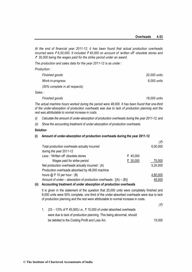
Overheads 4.53
At the end of financial year 2011-12, it has been found that actual production overheads
incurred were ` 6,00,000. It included ` 45,000 on account of ‘written off’ obsolete stores and
` 30,000 being the wages paid for the strike period under an award.
The production and sales data for the year 2011-12 is as under :
Production :
Finished goods 20,000 units
Work-in-progress 8,000 units
(50% complete in all respects)
Sales :
Finished goods 18,000 units
The actual machine hours worked during the period were 48,000. It has been found that one-third
of the under-absorption of production overheads was due to lack of production planning and the
rest was attributable to normal increase in costs.
(i) Calculate the amount of under-absorption of production overheads during the year 2011-12; and
(ii) Show the accounting treatment of under-absorption of production overheads.
Solution
(i) Amount of under-absorption of production overheads during the year 2011-12
(`) Total production overheads actually incurred 6,00,000
during the year 2011-12
Less : ‘Written off’ obsolete stores ` 45,000
Wages paid for strike period ` 30,000 75,000
Net production overheads actually incurred : (A) 5,25,000
Production overheads absorbed by 48,000 machine
hours @ ` 10 per hour : (B) 4,80,000
Amount of under – absorption of production overheads : [(A) – (B)] 45,000
(ii) Accounting treatment of under absorption of production overheads
It is given in the statement of the question that 20,000 units were completely finished and
8,000 units were 50% complete, one third of the under-absorbed overheads were due to lack
of production planning and the rest were attributable to normal increase in costs.
(`)
1. (33 – 1/3% of ` 45,000) i.e., ` 15,000 of under-absorbed overheads
were due to lack of production planning. This being abnormal, should
be debited to the Costing Profit and Loss A/c. 15,000
© The Institute of Chartered Accountants of India

4.54 Cost Accounting
2. Balance (66–2/3% of ` 45,000) i.e., ` 30,000 of under-absorbed
overheads should be distributed over work-in-progress, finished goods
and cost of sales by using supplementary rate. 30,000
Total under-absorbed overheads 45,000
Apportionment of unabsorbed overheads of ` 30,000 over, work-in progress, finished goods and cost of sales
Equivalent (`) Completed Units
Work-in-Progress 4,000 5,000
(4,000 units × ` 1.25)
(Refer to working note)
Finished goods 2,000 2,500
(2,000 units × ` 1.25)
Cost of sales 18,000 22,500
(18,000 units × ` 1.25)
24,000 30,000
Working Note:
Supplementary rate per unit = ` 30,000
24,000 = ` 1.25
4.8 Accounting and Control of Administrative Overheads
Definition - According to CIMA Terminology, Administrative overhead is defined as “The sum
of those costs of general management and of secretarial accounting and administrative
services, which cannot be directly related to the production, marketing, research or
development functions of the enterprise.” According to this definition, administrative overhead
constitutes the expenses incurred in connection with the formulation of policy directing the
organisation and controlling the operations of an undertaking. These overheads are also
collected and classified in the same way as the factory overheads.
4.8.1 Accounting of Administrative Overheads: There are three distinct methods of
accounting of administrative overheads, which are briefly discussed below:
(a) Apportioning Administrative Overheads between Production and Sales Departments:
According to this method administrative overheads are apportioned over production and sales
departments. The reason for the apportionment of overhead expenses over these
departments, recognises the fact that administrative overheads are incurred for the benefit of
both of these departments. Therefore each department should be charged with the proportion-
ate share of the same. When this method is adopted, administrative overheads lose their
identity and get merged with production and selling and distribution overheads.
© The Institute of Chartered Accountants of India
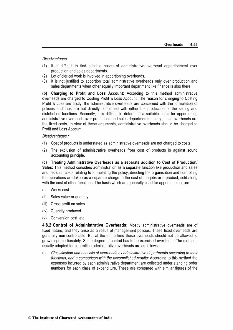
Overheads 4.55
Disadvantages:
(1) It is difficult to find suitable bases of administrative overhead apportionment over
production and sales departments.
(2) Lot of clerical work is involved in apportioning overheads.
(3) It is not justified to apportion total administrative overheads only over production and
sales departments when other equally important department like finance is also there.
(b) Charging to Profit and Loss Account: According to this method administrative
overheads are charged to Costing Profit & Loss Account. The reason for charging to Costing
Profit & Loss are firstly, the administrative overheads are concerned with the formulation of
policies and thus are not directly concerned with either the production or the selling and
distribution functions. Secondly, it is difficult to determine a suitable basis for apportioning
administrative overheads over production and sales departments. Lastly, these overheads are
the fixed costs. In view of these arguments, administrative overheads should be charged to
Profit and Loss Account.
Disadvantages :
(1) Cost of products is understated as administrative overheads are not charged to costs.
(2) The exclusion of administrative overheads from cost of products is against sound
accounting principle.
(c) Treating Administrative Overheads as a separate addition to Cost of Production/
Sales: This method considers administration as a separate function like production and sales
and, as such costs relating to formulating the policy, directing the organisation and controlling
the operations are taken as a separate charge to the cost of the jobs or a product, sold along
with the cost of other functions. The basis which are generally used for apportionment are:
(i) Works cost
(ii) Sales value or quantity
(iii) Gross profit on sales
(iv) Quantity produced
(v) Conversion cost, etc.
4.8.2 Control of Administrative Overheads: Mostly administrative overheads are of
fixed nature, and they arise as a result of management policies. These fixed overheads are
generally non-controllable. But at the same time these overheads should not be allowed to
grow disproportionately. Some degree of control has to be exercised over them. The methods
usually adopted for controlling administrative overheads are as follows:
(i) Classification and analysis of overheads by administrative departments according to their
functions, and a comparison with the accomplished results: According to this method the
expenses incurred by each administrative department are collected under standing order
numbers for each class of expenditure. These are compared with similar figures of the
© The Institute of Chartered Accountants of India

4.56 Cost Accounting
previous period in relation to accomplishment. Such a comparison will reveal efficiency
or inefficiency of the concerned department.
However, this method provides only a limited degree of control and comparison does not give
useful results if the level of activity is not constant during the periods under comparison. To
overcome this difficulty, overhead absorption rates may also be compared from period to
period; the extent of over or under absorption will reveal the efficiency or otherwise of the
department. It may be possible to compare the cost of a service department with that of
similar services obtainable from outside and a decision may be taken whether it is
economical to continue the department or entrust the work to outsiders.
(ii) Control through Budgets - According to this method, administration budgets (monthly or
annually) are prepared for each department. The budgeted figures are compared with
actual ones to determine variances. The variances are analysed and responsibility
assigned to the concerned department to control these variances.
(iii) Control through Standard - Under this method, standards of performance are fixed for
each administrative activity, and the actual performance is compared with the standards
set. In this way, standards serve not only as yardstick of performance but also facilitate
control of costs.
Illustration 20: (Reverse calculation of Factory overhead and Administrative overheads)
In an engineering company, the factory overheads are recovered on a fixed percentage basis
on direct wages and the administrative overheads are absorbed on a fixed percentage basis
on factory cost.
The company has furnished the following data relating to two jobs undertaken by it in a period:
Job 101 Job 102 (`) (`)
Direct materials 54,000 37,500
Direct wages 42,000 30,000
Selling price 1,66,650 1,28,250
Profit percentage on Total Cost 10% 20%
Required:
(i) Computation of percentage recovery rates of factory overheads and administrative
overheads.
(ii) Calculation of the amount of factory overheads, administrative overheads and profit for
each of the two jobs.
(iii) Using the above recovery rates fix the selling price of job 103. The additional data being:
Direct materials ` 24,000
© The Institute of Chartered Accountants of India

Overheads 4.57
Direct wages ` 20,000
Profit percentage on selling price 12-½%
Solution
(i) Let factory overhead recovery rate, as percentage of direct wages be F and
administrative overheads recovery rate, as percentage of factory cost be A.
Factory Cost of Jobs:
Job 101 = ` 96,000 + ` 42,000F
Job 102 = ` 67,500 + ` 30,000F
Total Cost of Production of Jobs:
Job 101 = (` 96,000 + ` 42,000F) + (` 96,000+ ` 42,000F) A = ` 1,51,500
Job-102 = (` 67,500 + ` 30,000F) + (` 67,500+ ` 30,000F) A = ` 1,06,875
(Refer to working note)
On solving above relations: F = 0.60 and A = 0.25
Hence, percentage recovery rates of factory overheads and administrative overheads are
60% and 25% respectively.
Working note:
Job 101 Job 102
Total cost of production (`) 1,51,500 1,06,875
Selling price
(100% Percentage of profit)+ (` 1,66,650/110%) (` 1,28,250/120%)
(ii) Statement of jobs, showing amount of factory overheads, administrative overheads
and profit
Job 101 Job 102
(`) (`) Direct materials 54,000 37,500
Direct wages 42,000 30,000
Prime cost 96,000 67,500
Factory overheads
60% of direct wages 25,200 18,000
Factory cost 1,21,200 85,500
Administrative overheads
25% of factory cost 30,300 21,375
Total cost 1,51,500 1,06,875
Profit 15,150 21,375
Selling price 1,66,650 1,28,250
© The Institute of Chartered Accountants of India

4.58 Cost Accounting
(iii) Selling price of Job 103
(`)
Direct materials 24,000
Direct wages 20,000
Prime cost 44,000
Factory overheads (60% of Direct Wages) 12,000
Factory cost 56,000
Administrative overheads 14,000
(25% of factory cost)
Total cost 70,000
Profit margin (balancing figure) 10,000
Selling price Total Cost
87.5%
80,000
4.9 Accounting and Control of Selling and Distribution Overheads
Selling cost or overhead expenses are the expenses incurred for the purpose of promoting the
marketing and sales of different products. Distribution expenses, on the other hand, are
expenses relating to delivery and dispatch of goods sold. Examples of selling and distribution
expenses have been considered earlier in this booklet. From the definitions it is clear that the
two type of expenses represent two distinct type of functions. Some concerns group together
these two type of overhead expenses into one composite class, namely, selling and
distribution overhead, for the purpose of Cost Accounting.
4.9.1 Accounting of selling and distribution overheads: The collection and
accumulation of each expense is made by means of appropriate standing order numbers in
the usual way. Where it is decided to apportion a part of the administrative overhead to the
selling division the same should also be collected through appropriate standing order
numbers.
As in the case of administrative overheads, it is not easy to determine an entirely satisfactory
basis for computing the overhead rate for absorbing selling overheads. The bases usually
adopted are:
(a) Sales value of goods;
(b) Cost of goods sold;
(c) Gross Profit on sales; and
(d) Number of orders or units sold.
It is considered that the sale value is ordinarily the most logical basis, there being some connection
between the amount of sales and the amount of expenses incurred to achieve them. The cost of
© The Institute of Chartered Accountants of India

Overheads 4.59
production, however, is not as satisfactory on basis as it may not have any direct relationship with
the selling and distribution cost.
The basis of gross profit on sales results in a larger share of the selling overhead being
applied to goods yielding a large margin of profit and vice versa. The basis therefore follows
the principle of ‘ability to pay, it may not reflect costs or incurred efforts.
An estimated amount per unit - The best method for absorbing selling and distributing expenses
over various products is to separate fixed expenses from variable expenses. Apportion the fixed
expenses according to the benefit derived by each product and thus ascertaining the fixed
expenses per unit. We give below some of the fixed expenses and the basis of apportionment:
Expenses Basis
Salaries in the Sales Department and of the sales men.
Estimated time devoted to the sale of various products.
Advertisement Actual amount incurred for each product since these days it is usual to advertise each product separately; common expenses, such as in an exhibition, should be apportioned on the basis of advertisement expenditure on each product.
Show Room expenses Average space occupied by each product.
Rent of finished goods godowns and Expenses on own delivery vans
Average quantities delivered during a period.
If a suitable basis for apportioning expenses does not exist it may be apportioned in the
proportion of sales of various products.
The total of fixed expenses apportioned in this manner, divided by the number of units sold or likely
to be sold, will give the fixed expenses per unit. To this should be added the variable expenses
which will be different for each product. These expenses are, packaging, freight outwards,
insurance in transit, commission payable to salesmen, rebate allowed to customers, etc. All these
items will be worked out per unit for each product separately. These items added to fixed expenses
per unit will give an estimated amount of the selling and distribution expenses per unit.
4.9.2 Control of Selling & Distribution Overheads: Control of selling and distribution
expenses is a difficult task. The reasons for this are as follows:
1. The incidence of selling and distribution overheads depends mainly on external factors,
such as distance of market, extent and nature of competition, terms of sales, etc. which
are beyond the control of management.
2. These overheads are dependent upon the customers, behaviour, their liking and
disliking, tastes etc. Therefore, as such control over the overheads may result in loss of
customers.
3. These expenses being of the nature of policy costs, are not amenable to control.
© The Institute of Chartered Accountants of India

4.60 Cost Accounting
In spite of the above difficulties, the following methods may be used for controlling them.
(a) Comparison with past performance - According to this method, selling and distribution
overheads are compared with the figures of the previous period. Alternatively, the expenses
may be expressed as a percentage of sales, and the percentages may be compared with
those of the past period. This method is suitable for small concerns.
(b) Budgetary Control - A budget is set up for selling and distribution expenses. The expenses
are classified into fixed and variable. If necessary, a flexible budget may be prepared indi-
cating the expenses at different levels of sales. The actual expenses are compared with the
budgeted figures and in the case of variances suitable actions are taken.
(c) Standard Costing - Under this method standards are set up in relation to the standard sales
volume. Standards may be set up for salesmen, territories, products etc. Once the
standards are set up, comparison is made between the actuals and standards : variances
are enquired into and suitable action taken.
Illustration 21: (Apportionment of Sales & Distribution overheads)
A company which sells four products, some of them unprofitable, proposes discontinuing the
sale of one of them. The following information is available regarding income, costs and activity
for the year ended 31st March, 2012.
Products
A B C D
Sales (` ) 3,00,000 5,00,000 2,50,000 4,50,000
Cost of sales (` ) 2,00,000 4,50,000 2,10,000 2,25,000
Area of storage (Sq.ft.) 50,000 40,000 80,000 30,000
Number of parcels sent 1,00,000 1,50,000 75,000 1,75,000
Number of invoices sent 80,000 1,40,000 60,000 1,20,000
Selling and Distribution overheads and the basis of allocation are:
Basis of allocation to products
Fixed Costs (`)
Rent & Insurance 30,000 Sq.Ft.
Depreciation 10,000 Parcel
Salesmen’s salaries & expenses 60,000 Sales Volume
Administrative wages and salaries 50,000 No. of invoices
Variable Costs :
Packing wages & materials ` 0.20 per parcel
Commission 4% of sales
Stationery ` 0.10 per invoice
© The Institute of Chartered Accountants of India

Overheads 4.61
You are required to prepare Profit & Loss Statement, showing the percentage of profit or loss
to sales for each product.
Solution
Statement of Profit or Loss on Various Products during the year ended March 31, 2012.
Products
Total A B C D
(`) (`) (`) (`) (`)
Sales 15,00,000 3,00,000 5,00,000 2,50,000 4,50,000
Variable costs
Cost of sales 10,85,000 2,00,000 4,50,000 2,10,000 2,25,000
Commissions 4% of sales 60,000 12,000 20,000 10,000 18,000
Packing wages &
materials @ ` 0.20 per parcel 1,00,000 20,000 30,000 15,000 35,000
Stationery @ ` 0.10 per invoice 40,000 8,000 14,000 6,000 12,000
Total variable costs 12,85,000 2,40,000 5,14,000 2,41,000 2,90,000
Contribution (Sales–
variable cost) 2,15,000 60,000 –14,000 9,000 1,60,000
Fixed Costs
Rent & Insurance (5:4:8:3) 30,000 7,500 6,000 12,000 4,500
Depreciation (4:6:3:7) 10,000 2,000 3,000 1,500 3,500
Salesmen’s salaries & expenses 60,000 12,000 20,000 10,000 18,000
(6:10:5:9)
Administrative wages & salaries
(4:7:3:6) 50,000 10,000 17,500 7,500 15,000
Total Fixed costs 1,50,000 31,500 46,500 31,000 41,000
Profit or Loss
(Contribution–fixed Costs) 65,000 28,500 –60,500 –22,000 1,19,000
Percentage of profit
or Loss on sales 4.3 9.5 –12.1 –8.8 26.4
4.10 Concepts Related to Capacity
(i) Installed/ Rated capacity: It refers to the maximum capacity of producing goods or
providing services. Installed capacity is determined either on the basis of technical
specification or through a technical evaluation. It is also known as theoretical capacity and is
© The Institute of Chartered Accountants of India

4.62 Cost Accounting
could not be achieved in normal operating circumstances.
(ii) Practical capacity: It is defined as actually utilised capacity of a plant. It is also known
as operating capacity. This capacity takes into account loss of time due to repairs, mainte-
nance, minor breakdown, idle time, set up time, normal delays, Sundays and holidays, stock
taking etc. Generally, practical capacity is taken between 80 to 90% of the rated capacity. It is
also used as a base for determining overhead rates. Practical capacity is also called net
capacity or available capacity.
(iii) Normal capacity: Normal capacity is the volume of production or services achieved or
achievable on an average over a period under normal circumstances taking into account the
reduction in capacity resulting from planned maintenance.
Normal capacity is determined as under:
Installed capacity xxx
Adjustments for:
(i) Time lost due to scheduled preventive or planned maintenance
xxx
(ii) Number of shifts or machine hours or man hours
(iii) Holidays, normal shut down days, normal idle time xxx
(iv) Normal time lost in batch change over xxx xxx
Normal Capacity xxx
(iv) Actual capacity: It is the capacity actually achieved during a given period. It is
presented as a percentage of installed capacity.
(v) Idle capacity: It is that part of the capacity of a plant, machine or equipment which
cannot be effectively utilised in production.
(a) Normal Idle Capacity: It is the difference between Installed capacity and Normal
capacity.
(b) Abnormal Idle Capacity: It is the difference between Normal capacity and Actual
capacity utilization where the actual capacity is lower than the normal capacity.
The idle capacity may arise due to lack of product demand, non-availability of raw material,
shortage of skilled labour, absenteeism, shortage of power fuel or supplies, seasonal nature of
product etc.
Installed Capacity
Normal Idle Capacity
Normal Capacity
Abnormal Idle Capacity
Actual Capacity
© The Institute of Chartered Accountants of India

Overheads 4.63
Treatment of Idle capacity costs: Idle capacity costs can be treated in product costing, in the
following ways :
(a) If the idle capacity cost is due to unavoidable reasons such as repairs, maintenance,
changeover of job etc. a supplementary overhead rate may be used to recover the idle
capacity cost. In this case, the costs are charged to the production capacity utilised.
(b) If the idle capacity cost is due to avoidable reasons such as faulty planning, power failure
etc.; the cost should be charged to costing profit and loss account.
(c) If the idle capacity cost is due to seasonal factors, then, the cost should be charged to
the cost of production by inflating overhead rates.
4.11 Treatment of Certain Items in Costing
(i) Interest and financing charges: It includes any payment in nature of interest for use of
non equity funds and incidental cost that an entity incurs in arranging those funds. Example of
interest and financing charges are interest on borrowings, financing charges in respect of
finance leases, cash discount allowed to customers. The term interest and financing charges,
finance costs and borrowing costs are used interchangeably. It does not include imputed
costs.
Interest and financing charges shall be presented in the cost statement as a separate item of
cost of sales.
(ii) Depreciation: Depreciation “is the diminution in the intrinsic value of an asset due to use
and/or the lapse of time.” Depreciation is thus the result of two factors viz., the use, and the
lapse of time. We know that each fixed asset loses its intrinsic value due to their continuous
use and as such the greater the use the higher is the amount of depreciation. The loss in the
intrinsic value may also arise even if the asset in question is not in service.
Assignment of Depreciation:
It shall be traced to the cost object to the extent economically feasible. Where it is not directly
traceable it should be assigned using either or two principles i.e. (i) Cause and Effect and (ii)
Benefit received.
(iii) Packing expenses: Cost of primary packing necessary for protecting the product or for
convenient handling, should become a part of the prime cost. The cost of packing to facilitate the
transportation of the product from the factory to the customer should become a part of the
distribution cost. If the cost of special packing is at the request of the customer, the same should
be charged to the specific work order or the job. The cost of fancy packing necessary to attract
customers is an advertising expenditure. Hence, it is to be treated as a selling overhead.
(iv) Fringe benefits: These are the additional payments or facilities provided to the workers
apart from their salary and direct cost-allowances like house rent, dearness and city compen-
satory allowances. These benefits are given in the form of overtime, extra shift duty allowance,
holiday pay, pension facilities etc.
© The Institute of Chartered Accountants of India

4.64 Cost Accounting
These indirect benefits stand to improve the morale, loyalty and stability of employees towards the
organisation. If the amount of fringe benefit is considerably large, it may be recovered as direct
charge by means of a supplementary wage or labour rate; otherwise these may be collected as
part of production overheads.
(v) Expenses on removal and re-erection of machines: Expenses are sometime incurred
on removal and re-erection of machinery in factories. Such expenses may be incurred due to
factors like change in the method of production; an addition or alteration in the factory
building, change in the flow of production, etc. All such expenses are treated as production
overheads. When amount of such expenses is large, it may be spread over a period of time.
If such expenses are incurred due to faulty planning or some other abnormal factor, then they
may be charged to costing Profit and Loss Account.
(vi) Bad debts: There is no unanimity among different authors of Cost Accounting about the
treatment of bad debts. One view is that ‘bad debts’ should be excluded from cost. According
to this view bad debts are financial losses and therefore, they should not be included in the
cost of a particular job or product.
According to another view it should form part of selling and distribution overheads, especially
when they arise in the normal course of trading. Therefore bad debts should be treated in cost
accounting in the same way as any other selling and distribution cost. However extra ordinarily
large bad debts should not be included in cost accounts.
(vii) Training expenses: Training is an essential input for industrial workers. Training expenses in
fact includes wages of workers, costs incurred in running training department, loss arising from the
initial lower production, extra spoilage etc. Training expenses of factory workers are treated as part
of the cost of production. The training expenses of office; sales or distribution workers should be
treated as office; sales or distribution overhead as the case may be. These expenses can be
spread over various departments of the concern on the basis of the number of workers on roll.
Training expenses would be abnormally high in the case of high labour turnover such
expenses should be excluded from costs and charged to the costing profit and loss account.
(viii) Canteen expenses: The subsidy provided or expenses borne by the firm in running the
canteen should be regarded as a production overhead. If the canteen is meant only for factory
workers therefore this expenses should be apportioned on the basis of the number of workers
employed in each department. If office workers also take advantage of the canteen facility, a
suitable share of the expenses should be treated as office overhead.
(ix) Carriage and cartage expenses: It includes the expenses incurred on the movement
(inward and outwards) and transportation of materials and goods. Transportation expenses
related to direct material may be included in the cost of direct material and those relating to
indirect material (stores) may be treated as factory overheads. Expenses related to the
transportation of finished goods may be treated as distribution overhead.
(x) Expenses for welfare activities: All expenses incurred on the welfare activities of
employees in a company are part of general overheads. Such expenses should be
© The Institute of Chartered Accountants of India

Overheads 4.65
apportioned between factory, office, selling and distribution overheads on the basis of number
of persons involved.
(xi) Night shift allowance: Workers in the factories, which operate during night time are paid
some extra amount known as ‘night shift allowance’. This extra amount is generally incurred
due to the general pressure of work beyond normal capacity level and is treated as production
overhead and recovered as such.
If this allowance is treated as part of direct wages, the jobs/production carried at night will be
costlier than jobs/production performed during the day. However, if additional expenditure on
night shift is incurred to meet some specific customer order, such expenditure may be charged
directly to the order concerned. If night shifts are run due to abnormal circumstances, the
additional expenditure should be charged to the costing profit and loss account.
(xii) Research and Development Expenses: The Terminology defines research expenses as
“the expenses of searching for new or improved products, new application of materials, or new
or improved methods.” Similarly, development expenses are defined as “the expenses of the
process which begins with the implementation of the decision to produce a new or improved
product.”
If research is conducted in the methods of production, the research expenses should be
charged to the production overhead; while the expenditure becomes a part of the
administration overhead if research relates to administration. Similarly, market research
expenses are charged to the selling and distribution overhead.
Development costs incurred in connection with a particular product should be charged directly
to that product. Such expenses are usually treated as “deferred revenue expenses,” and
recovered as a cost per unit of the product when production is fully established.
General research expenses of a routine nature incurred on new or improved methods of
manufacture or the improvement of the existing products should be charged to the general
overhead.
Even in this case, if the amount involved is substantial it may be treated as a deferred revenue
expenditure, and spread over the period during which the benefit would accrue. Expenses on
fundamental research, not relating to any specific product, are treated as a part of the
administration overhead. Where research proves a failure, the cost associated with it should
be excluded from costs and charged to the costing Profit and Loss Account.
4.12 Summary
1. Overheads represent expenses that have been incurred in providing certain ancillary
facilities or services which facilitate or make possible the carrying out of the production
process; by themselves these services are not of any use.
2. Overheads can be classified in to four types on the basis of function-
• Factory or Manufacturing Overheads
© The Institute of Chartered Accountants of India

4.66 Cost Accounting
• Office and Administration Overheads
• Selling and Distribution Overheads
• Research and Development Overheads
3. Overheads can be classified in to three types on the basis of nature-
• Fixed Overhead- Expenses that are not affected by any variation in the volume of
activity.
• Variable- Expenses that change in proportion to the change in the volume of activity.
• Semi variable- The expenses that do not change when there is a small change in
the level of activity but change whenever there is a slightly big change or change in
the same direction as change in the level of activity but not in the same proportion.
4. Cost allocation- The term ‘allocation’ refers to assignment or allotment of an entire item
of cost to a particular cost center or cost unit.
5. Cost apportionment- Apportionment implies the allotment of proportions of items of cost
to cost centres or departments.
6. Re-apportionment- The process of assigning service department overheads to
production departments is called reassignment or re-apportionment.
7. Absorption- The process of recovering overheads of a department or any other cost
center from its output is called recovery or absorption.
8. Following are the methods used for re-apportionment of service department expenses
over the production departments-
• Direct re-distribution method- Under this method service department costs are
apportioned over the production departments only, ignoring the services rendered
by one service department to the other.
• Step Method or Non-reciprocal method- This method gives cognizance to the
service rendered by service department to another service department. The
sequence here begins with the department that renders service to the maximum
number of other service departments.
• Reciprocal Service Method- These methods are used when different service
departments render services to each other, in addition to rendering services to
production departments. In such cases various service departments have to share
overheads of each other. The methods available for dealing with reciprocal services are
(a) Simultaneous equation method;
(b) Repeated distribution method;
(c) Trial and error method.
© The Institute of Chartered Accountants of India

Overheads 4.67
9. Blanket overhead rates- Blanket overhead rate refers to the computation of one single
overhead rate for the whole factory. It is to be distinguished from the departmental overhead
rate which refers to a separate rate for each individual cost centre or department.
Blanket Overhead rate =Overhead costs for the whole factory
×100Total units of the selected base
10. Percentage of direct material
Overhead rate =Total Production Overheads of a Department
×100Budgeted Direct Material cost of all products
11. Percentage of prime cost
Overhead rate =Total Production Overheads of a Department
×100Budgeted Prime Cost
12. Percentage of direct labour cost
Direct Labour Cost Percentage Rate
=Total Production Overheads of a Department
×100Budgeted Direct Labour Cost
• Labour hour rate
Direct Labour Hour Rate =Total Production Overheads of a Department
Budgeted Direct labour Hours
• Machine hour rate
Direct Machine Hour Rate =Total Production Overheads of a Department
Budgeted Machine Hours
13. Methods of accounting of administrative overheads
• Apportioning Administrative Overheads between Production and Sales Departments.
• Charging to Costing Profit and Loss Account.
• Treating Administrative Overheads as a separate addition to Cost of Production/Sales
• The basis which are generally used for apportionment are :
(i) Works cost
(ii) Sales value or quantity
(iii) Gross profit on sales
(iv) Quantity produced
(v) Conversion cost, etc.
© The Institute of Chartered Accountants of India
5 Non-Integrated Accounts
Learning Objectives
After studying this chapter you should be able to
Differentiate between integrated and non-integrated systems of accounting
Identify the ledgers maintained by financial as well as cost departments
Understand the reasons for differences between financial and cost accounts
Prepare a reconciliation statement accordingly and
Should be in a position to write the various journal entries for both integrated and non-
integrated systems of accounting.
5.1 Introduction
To operate business operations efficiently and successfully, it is necessary to make use of an
appropriate accounting system. Such a system should state in clear terms whether cost and
financial transactions should be integrated or kept separately (Non-integrated). Where cost and
financial accounting records are integrated, the system so evolved is known as integrated or
integral accounting. In case cost and financial transactions are kept separately, the system is
called Non-Integrated Accounting or Cost control System. While non-integrated system of
accounting necessitates reconciliation between financial and cost accounts, no reconciliation
between two sets of accounts is required under integrated accounting.
5.2 Non-Integrated Accounting System
It is a system of accounting under which separate ledgers are maintained for cost and financial
accounts by Accountants. This system is also referred to as cost ledger accounting system. Under
such a system the cost accounts restricts itself to recording only those transactions which relate to
the product or service being provided. Hence items of expenses which have a bearing with sales
or, production or for that matter any other items which are under the factory management are the
ones dealt with in such accounts. This leads to the exclusion of certain expenses like interest, bad
debts and revenue/income from ‘other than the sale of product or service’.
A special feature of the non-integrated system of accounts is its ability to deal with notional
© The Institute of Chartered Accountants of India

5.2 Cost Accounting
expenses like rent or interest on capital tied up in the stock. The accounting of notional rent
facilitates comparisons amongst factories (some owned and some rented).
Non-Integrated Accounting Systems contain fewer accounts when compared with financial
accounting because of the exclusion of purchases, expenses and also Balance Sheet items like
fixed assets, debtors and creditors. Items of accounts which are excluded are represented by an
account known as Cost ledger control account.
The important ledgers to be maintained under non-integrated accounting system in the Cost
Accounting department are the following:
(a) Cost Ledger - This is the principle ledger of the cost department in which impersonal
accounts are recorded. This ledger is made self-balancing by maintaining therein a Control
Account for each subsidiary ledger.
(b) Stores Ledger - It contains an account for each item of stores. The entries in each account
maintained in this ledger are made from the invoice, goods received note, material requisitions,
material received note etc. Accounts in respect of each item of stores show receipt, issue and
balance in physical as well as in monetary terms.
(c) Work-in-Progress Ledger - This ledger is also known as job ledger, it contains accounts of
unfinished jobs and processes. All material costs, wages and overheads for each job in progress
are posted to the respective job account in this ledger. The balance in a job account represents
total balance of job/work-in-progress, as shown by the job account.
(d) Finished Goods Ledger - It contains an account for each item of finished product
manufactured or the completed job. If the finished product is transferred to stores, a credit entry is
made in the work-in-progress ledger and a corresponding debit entry is made in this ledger.
5.2.1 Principal Accounts : The main accounts which are usually prepared when a separate
Cost Ledger is maintained are as follows :
(1) Cost Ledger Control Account - This account is also known as General Ledger Adjustment
Account. This account is made to complete double entry. All items of expenditure are
credited to this account. Sales are debited to this account and net profit/loss is transferred to
this account. The balance in this account at the end of the particular period represents the
net total of all the balances of the impersonal account
(2) Stores Ledger Control Account –This account is debited for the purchase of material and
credited for issue of materials from stores. The balance in this account indicates the total
balance of all the individual stores accounts. Abnormal losses or gains if any in this account,
are transferred to Costing Profit & Loss Account. Entries are made on the basis of goods
received notes and stores requisitions etc.
(3) Wage Control Account - This account is debited with total wages paid (direct and indirect).
Direct wages are further transferred to Work-in-Progress Account and indirect wages to
Production Overhead; Administration Overhead or Selling & Distribution Overhead Account,
as the case may be. Wages paid for abnormal idle time are transferred to Costing Profit &
© The Institute of Chartered Accountants of India

Non-Integrated Accounts 5.3
Loss Account either directly or through Abnormal Loss Account.
(4) Manufacturing/Production/Works Overhead Control Account - This account is debited
with indirect costs of production such as indirect material, indirect labour, indirect expenses
(carriage inward etc.). Overhead recovered is credited to this Account. The difference
between overhead incurred and overhead recovered (i.e. Under Absorption or Over
Absorption of Overheads) is transferred to Overhead Adjustment Account.
(5) Work-in-Progress Control Account - This account is debited with the total cost of
production, which includes—direct materials, direct labour, direct expenses, production
overhead recovered, and is credited with the amount of finished goods completed and
transferred. The balance in this account represents total balances of jobs/works-in-progress,
as shown by several job accounts.
(6) Administrative Overhead Control Account - This account is debited with overhead
incurred and credited with Overhead recovered. The Overhead recovered are debited to
Finished Goods Account. The difference between Administrative Overhead incurred and
recovered is transferred to Overhead Adjustment Account.
(7) Finished Goods Control Accounts - This account is debited with the value of goods
transferred from work-in-progress account, administration costs recovered. This account is
credited with the cost of goods sold and Cost of Sales Account is debited. The balance of
this account represents the value of goods lying at hand.
(8) Selling and Distribution Overhead Account - This account is debited with Selling and
Distribution Overhead incurred and credited with the recovered Overhead. The difference
between incurred and recovered overhead is transferred usually to Overhead Adjustment
Account.
(9) Cost of Sales Account - This account is debited with the cost of finished goods transferred
from Finished Goods Account for sale as well as with the amount of selling and distribution
overhead costs recovered. The balance of this account is ultimately transferred to Sales
Account or Costing Profit & Loss Account.
(10) Costing Profit & Loss Account – This account is debited with cost of goods sold, under-
absorbed overheads and abnormal losses. And is credited with sales value, over-absorbed
overhead and abnormal gains. The net profit or loss in this account is transferred to Cost
Ledger Control Account.
(11) Overhead Adjustment Account - This account is to be debited for under-recovery of
overhead and credited with over-recovery of overhead amount. The net balance in this
account is transferred to Costing Profit & Loss Account.
Note: Sometimes, Overhead Adjustment Account is dispensed with and under/over absorbed
overheads is directly transferred to Costing Profit & Loss Account from the respective
overhead accounts.
© The Institute of Chartered Accountants of India

5.4 Cost Accounting
5.2.2 Scheme of Entries; The manner in which the Cost Ledger, when maintained on a
double entry basis, would operate is illustrated by the following statements of various journal
entries as would appear in the cost books.
Material:
(a) Purchase—` 5,000 (credit or cash) (`) (`)
(i) Material Control A/c …………………………….. Dr. 5,000
To Cost Ledger Control A/c 5,000
(ii) Stores Ledger Control A/c ……………………… Dr. 5,000
To Material Control A/c 5,000
Note: Sometimes Material Control Account is dispensed with and entries are directly made into
Stores Ledger Control A/c, giving a credit to Cost Ledger Control A/c.
(b) Purchases worth ` 500 for special job
Work-in-Progress Ledger Control A/c…………………. Dr. 500
To Cost Ledger Control A/c 500
(c) Material returned to vendor—` 500
Cost Ledger Control A/c …………………………………. Dr. 500
To Store Ledger Control A/c 500
(d) (i) Material (Direct) issued to production—` 1,000
Work-in-Progress Control A/c……………………. Dr. 1,000
To Store Ledger Control A/c 1,000
(ii) Material (Indirect) issued to production—` 200
Manufacturing Overhead A/c…………………. Dr. 200
To Store Ledger Control A/c 200
(e) (i) Material worth ` 200 returned from shop to stores
Stores Ledger Control A/c…………………. Dr. 200
To Work-in-Progress Control A/c 200
(ii) Material worth ` 100 is transferred from Job-1 to Job- 2
Job- 2 A/c………………………………………… Dr. 100
To Job- 1 A/c 100
(f) Material worth ` 100 is issued from stores for repairs
Manufacturing Overhead A/c……………………………. Dr. 100
To Stores Ledger Control A/c 100
Labour:
(g) Direct wages paid to workers— ` 1,000
Wages Control A/c………………………………………… Dr. 1,000
To Cost Ledger Control A/c 1,000
© The Institute of Chartered Accountants of India

Non-Integrated Accounts 5.5
(h) Indirect wages paid to workers in the production— ` 700
(i) Wages Control A/c……………………………………… Dr. 700
To Cost Ledger Control A/c 700
(ii) Production Overhead A/c……………………………. Dr. 700
To Wages Control A/c 700
(i) Indirect wages paid to workers in administration— ` 500
(i) Wages Control A/c……………………………………… Dr. 500
To Cost Ledger Control A/c 500
(ii) Administration Overhead A/c………………………… Dr. 500
To Wages Control A/c 500
(j) Indirect wages paid to workers in Selling & Dist. department— ` 300
(i) Wages Control A/c……………………………………… Dr. 300
To Cost Ledger Control A/c 300
(ii) Selling & Dist. Overhead A/c…………………………. Dr. 300
To Wages Control A/c 300
Direct Expenses:
(k) Direct expenses incurred ` 500 for Job No. 12
Job No. 12 A/c (WIP Control A/c)………………………. Dr. 500
To Cost Ledger Control A/c 500
Overheads:
(l) Overhead expenses incurred ` 500 (Production `150;
Administrative `150; Selling and Distribution `200)
Production Overhead Control A/c……………………….. Dr. 150
Administrative Overhead Control A/c…………………… Dr 150
Selling & Dist. Overhead Control A/c…………………… Dr 200
To Cost Ledger Control A/c 500
(m) Carriage Inward—` 100
Manufacturing Overhead A/c…………………………….. Dr. 100
To Cost Ledger Control A/c 100
(n) Production overhead recovered—` 1,000
Work-in-Progress Ledger Control A/c…………………... Dr. 1,000
To Production Overhead A/c 1,000
(o) Administrative Overhead recovered ` 500 from finished goods
Finished Goods Ledger Control A/c…………………….. Dr. 500
To Administrative Overhead A/c 500
© The Institute of Chartered Accountants of India

5.6 Cost Accounting
(p) Selling and Distribution Overhead ` 100 recovered from sales
Cost of Sales A/c………………………………………….. Dr. 100
To Selling & Dist. Overhead A/c 100
(q) Under recovery of overheads
Costing Profit & Loss A/c…………………………………. Dr. xxx
To Administrative Overhead A/c xxx
(r) Over recovery of overheads
Production Overheads A/c……………………………….. Dr. xxx
To Costing Profit & Loss A/c xxx
Sales:
(s) Cost Ledger Control A/c………………………………….. Dr. xxx
To Costing Profit & Loss A/c xxx
Profit/ Loss:
(t) In case of Profit
(i) Costing Profit & Loss A/c…………………………… Dr. xxx
To Cost Ledger Control A/c xxx
(u) In case of Loss
(ii) Cost Ledger Control A/c…………………………… Dr. xxx
To Costing Profit & Loss A/c xxx
Non-Integrated Accounting System-flowchart
© The Institute of Chartered Accountants of India

Non-Integrated Accounts 5.7
Illustration 1: (Non-Integrated accounts journal entries)
As on 31st March, 2013, the following balances existed in a firm’s Cost Ledger:
Dr. Cr.
(`) (`)
Stores Ledger Control A/c 3,01,435
Work-in-Progress Control A/c 1,22,365
Finished Stock Ledger Control A/c 2,51,945
Manufacturing Overhead Control A/c 10,525
Cost Ledger Control A/c 6,65,220
6,75,745 6,75,745
During the next three months the following items arose:
(`)
Finished product (at cost) 2,10,835
Manufacturing overhead incurred 91,510
Raw materials purchased 1,23,000
Factory Wages 50,530
Indirect Labour 21,665
Cost of Sales 1,85,890
Material issued to production 1,27,315
Sales returned at Cost 5,380
Material returned to suppliers 2,900
Manufacturing overhead charged to production 77,200
You are required to pass the Journal Entries; write up the accounts and schedule the balances, stating what each balance represents.
Solution:
Journal entries are as follows:
Dr. Cr.
(`) (`)
1. Finished stock ledger Control A/c…………………….. Dr. 2,10,835
To Work-in-Progress Control A/c 2,10,835
2. Manufacturing Overhead Control A/c………………… Dr. 91,510
To Cost Ledger Control A/c 91,510
3. Stores Ledger Control A/c……………………………... Dr. 1,23,000
To Cost Ledger Control A/c 1,23,000
© The Institute of Chartered Accountants of India

5.8 Cost Accounting
4. (i) Wage Control A/c……………………………………. Dr. 72,195
To Cost Ledger Control A/c 72,195
(ii) Work-in-progress Control A/c……………………... Dr. 50,530
To Wages Control A/c 50,530
(iii) Manufacturing Overhead Control A/c……………. Dr. 21,665
To Wages Control A/c 21,665
5. Cost of Sales A/c………………………………………... Dr. 1,85,890
To Finished Stock Ledger A/c 1,85,890
6. Work-in-Progress Control A/c…………………………. Dr. 1,27,315
To Stores Ledger Control A/c 1,27,315
7. Finished Stock Ledger Control A/c…………………… Dr. 5,380
To Cost of Sales A/c 5,380
8. Cost Ledger Control A/c……………………………….. Dr. 2,900
To Stores Ledger Control A/c 2,900
9. Work-in-Progress Control A/c…………………………. Dr. 77,200
To Manufacturing Overhead Control A/c 77,200
COST LEDGER
Cost Ledger Control Account
(`) (`)
To Stores Ledger Control A/c (return)
2,900 By Balance b/d 6,65,220
” Balance c/d 9,49,025 ” Manufacturing OH Control A/c 91,510
” Stores Ledger Control A/c 1,23,000
” Wages Control A/c 72,195
9,51,925 9,51,925
Stores Ledger Control Account
(`) (`)
To Balance b/d 3,01,435 By Work in Progress Control A/c 1,27,315
” Cost Ledger Control A/c 1,23,000 ” Cost Ledger Control A/c 2,900
” Balance c/d 2,94,220
4,24,435 4,24,435
© The Institute of Chartered Accountants of India

Non-Integrated Accounts 5.9
Work-in-Progress Control Account
(`) (`)
To Balance b/d 1,22,365 By Finished Stock Ledger Control A/c
2,10,835
” Wages Control A/c 50,530 ” Balance c/d 1,66,575
Stores Ledger Control A/c 1,27,315
Manufacturing OH Control A/c 77,200
3,77,410 3,77,410
Finished Stock Ledger Control Account
(`) (`)
To Balance b/d 2,51,945 By Cost of Sales Control A/c 1,85,890
” Work in Progress Control A/c 2,10,835 ” Balance c/d 2,82,270
” Cost of Sales Control A/c (Return at cost)
5,380
4,68,160 4,68,160
Manufacturing Overhead Control Account
(`) (`)
To Cost Ledger Control A/c 91,510 By Balance b/d 10,525
” Wages Control A/c 21,665 ” Work in Progress Control A/c 77,200
” Balance c/d 25,450
1,13,175 1,13,175
Wages Control Account
(`) (`)
To Cost Ledger Control A/c 72,195 By Work in Progress Control A/c 50,530
” Manufacturing OH Control A/c
21,665
72,195 72,195
Cost of Sales Account
(`) (`)
To Finished Stock Ledger Control
1,85,890 By Finished Stock Ledger Control (Return)
5,380
” Balance c/d 1,80,510
1,85,890 1,85,890
© The Institute of Chartered Accountants of India

5.10 Cost Accounting
Trial Balance
Dr. Cr.
(`) (`)
Stores Ledger Control A/c 2,94,220
Work-in-Progress Control A/c 1,66,575
Finished Stock Ledger Control A/c 2,82,270
Manufacturing Overhead Control A/c 25,450
Cost of Sales A/c 1,80,510
Cost Ledger Control A/c 9,49,025
9,49,025 9,49,025
Illustration 2: (Preparation of condensed P&L statement and supporting schedules)
The following figures are extracted from the Trial Balance of Go-getter Co. on 30th September, 2012:
Dr. Cr.
(`) (`)
Inventories:
Finished Stock 80,000
Raw Materials 1,40,000
Work-in-Progress 2,00,000
Office Appliances 17,400
Plant & Machinery 4,60,500
Building 2,00,000
Sales 7,68,000
Sales Return and Rebates 14,000
Materials Purchased 3,20,000
Freight incurred on Materials 16,000
Purchase Returns 4,800
Direct Labour 1,60,000
Indirect Labour 18,000
Factory Supervision 10,000
Repairs and Upkeep Factory 14,000
Heat, Light and Power 65,000
© The Institute of Chartered Accountants of India

Non-Integrated Accounts 5.11
Rates and Taxes 6,300
Miscellaneous Factory Expenses 18,700
Sales Commission 33,600
Sales Travelling 11,000
Sales Promotion 22,500
Distribution Deptt.—Salaries and Expenses 18,000
Office Salaries and Expenses 8,600
Interest on Borrowed Funds 2,000
Further details are available as follows:
(i) Closing Inventories:
Finished Goods 1,15,000
Raw Materials 1,80,000
Work-in-Progress 1,92,000
(ii) Accrued expenses on:
Direct Labour 8,000
Indirect Labour 1,200
Interest on Borrowed Funds 2,000
(iii) Depreciation to be provided on:
Office Appliances 5%
Plant and Machinery 10%
Buildings 4%
(iv) Distribution of the following costs:
Heat, Light and Power to Factory, Office and Distribution in the ratio 8 : 1 : 1.
Rates and Taxes two-thirds to Factory and one-third to Office.
Depreciation on Buildings to Factory, Office and Selling in the ratio 8 : 1 : 1.
With the help of the above information, you are required to prepare a condensed Profit and
Loss Statement of Go-getter Co. for the year ended 30th September, 2012 along with
supporting schedules of:
(i) Cost of Sales.
(ii) Selling and Distribution Expenses.
(iii) Administration Expenses.
© The Institute of Chartered Accountants of India

5.12 Cost Accounting
Solution:
Profit and Loss Statement of Go-getter Company
for the year ended 30th September, 2012
(`) (`)
Gross Sales 7,68,000
Less: Returns (14,000) 7,54,000
Less: Cost of Sales [Refer to Schedule (i)] (7,14,020)
Net Operating Profit 39,980
Less: Interest on borrowed funds (4,000)
Net Profit 35,980
(i) Schedule of Cost of Sales
(`) (`)
Raw Material (Inventory opening balance) 1,40,000
Add: Material Purchased 3,20,000
Add: Freight on Material 16,000
Less: Purchase Returns (4,800) 3,31,200
4,71,200
Less: Closing Raw Material Inventory (1,80,000)
Materials consumed in Production 2,91,200
Direct Labour (`1,60,000 + `8,000) 1,68,000
Prime Cost 4,59,200
Factory Overheads:
Indirect Labour (`18,000 + `1,200) 19,200
Factory Supervision 10,000
Repairs and Factory Upkeep 14,000
Heat, Light and Power (`65,000 × 8/10) 52,000
Rates and Taxes (`6,300 × 2/3rd) 4,200
Miscellaneous Factory Expenses 18,700
Depreciation of Plant (10% of `4,60,500) 46,050
Depreciation of Buildings (4% of `2,00,000 × 8/10) 6,400 1,70,550
Gross Works cost 6,29,750
© The Institute of Chartered Accountants of India

Non-Integrated Accounts 5.13
Add: Opening Work-in-Process inventory 2,00,000
Less: Closing Work-in-Process inventory (1,92,000)
Works Cost 6,37,750
Add: Opening Finished Goods inventory 80,000
Less: Closing Finished Goods inventory (1,15,000)
Cost of Production 6,02,750
Add: Administration Expenses [See Schedule (iii)] 18,870
Cost of Goods Sold 6,21,620
Add: Selling and Distribution Expenses [See Schedule (ii)] 92,400
Cost of Sales 7,14,020
(ii) Schedule of Selling and Distribution Expenses
(`)
Sales Commission 33,600
Sales Travelling 11,000
Sales Promotion 22,500
Distribution Deptt.—Salaries and Expenses 18,000
Heat, Light and Power 6,500
Depreciation of Buildings 800
92,400
(iii) Schedule of Administration Expenses
(`)
Office Salaries and Expenses 8,600
Depreciation of Office Appliances 870
Depreciation of Buildings 800
Heat, Light and Power 6,500
Rates and Taxes 2,100
18,870
Illustration 3: (Preparation of ledger as per integrated accounting system)
In the absence of the Chief Accountant, you have been asked to prepare a month’s cost
accounts for a company which operates a batch costing system fully integrated with the
financial accounts. The following relevant information is provided to you:
© The Institute of Chartered Accountants of India

5.14 Cost Accounting
(`) (`)
Balances at the beginning of the month:
Stores Ledger Control Account 25,000
Work-in-Progress Control Account 20,000
Finished Goods Control Account 35,000
Prepaid Production Overheads brought forward from previous month
3,000
Transactions during the month:
Materials Purchased 75,000
Materials Issued:
To Production 30,000
To Factory Maintenance 4,000 34,000
Materials transferred between batches 5,000
Total wages paid:
To Direct workers 25,000
To Indirect workers 5,000 30,000
Direct wages charged to batches 20,000
Recorded non-productive time of direct workers 5,000
Selling and Distribution Overheads Incurred 6,000
Other Production Overheads Incurred 12,000
Sales 1,00,000
Cost of Finished Goods Sold 80,000
Cost of Goods completed and transferred into finished goods during the month
65,000
Physical value of work-in-progress at the end of the month 40,000
The production overhead absorption rate is 150% of direct wages charged to work-in-
progress.
Required:
Prepare the following accounts for the month:
(a) Stores Ledger Control Account.
(b) Work-in-Progress Control Account.
© The Institute of Chartered Accountants of India
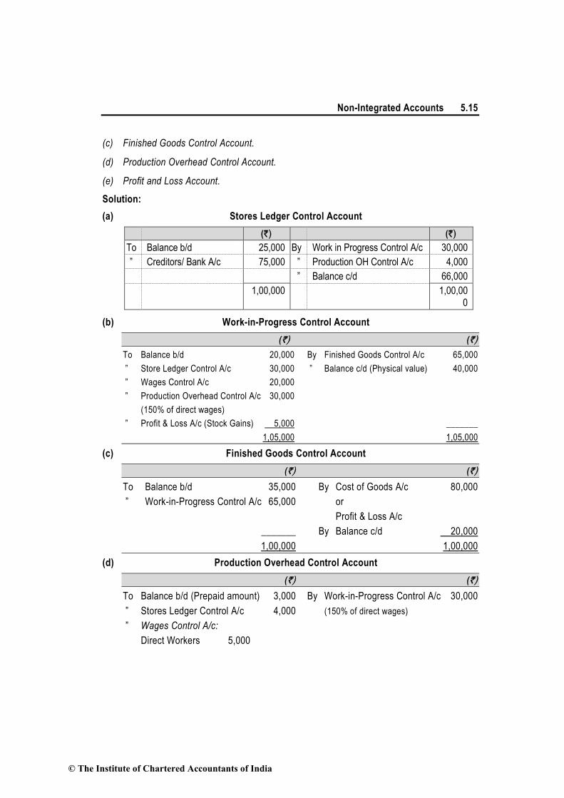
Non-Integrated Accounts 5.15
(c) Finished Goods Control Account.
(d) Production Overhead Control Account.
(e) Profit and Loss Account.
Solution:
(a) Stores Ledger Control Account
(`) (`)
To Balance b/d 25,000 By Work in Progress Control A/c 30,000
” Creditors/ Bank A/c 75,000 ” Production OH Control A/c 4,000
” Balance c/d 66,000
1,00,000 1,00,000
(b) Work-in-Progress Control Account
(`) (`)
To Balance b/d 20,000 By Finished Goods Control A/c 65,000
” Store Ledger Control A/c 30,000 ” Balance c/d (Physical value) 40,000
” Wages Control A/c 20,000
” Production Overhead Control A/c 30,000
(150% of direct wages)
” Profit & Loss A/c (Stock Gains) 5,000 _______
1,05,000 1,05,000
(c) Finished Goods Control Account
(`) (`)
To Balance b/d 35,000 By Cost of Goods A/c 80,000
” Work-in-Progress Control A/c 65,000 or
Profit & Loss A/c
_______ By Balance c/d 20,000
1,00,000 1,00,000
(d) Production Overhead Control Account
(`) (`)
To Balance b/d (Prepaid amount) 3,000 By Work-in-Progress Control A/c 30,000
” Stores Ledger Control A/c 4,000 (150% of direct wages)
” Wages Control A/c:
Direct Workers 5,000
© The Institute of Chartered Accountants of India

5.16 Cost Accounting
Indirect Workers 5,000 10,000
” Bank 12,000
” Profit & Loss A/c* 1,000
(Over absorption, balancing figure)______ ______
30,000 30,000
* Alternatively the over absorbed overhead may be carried forward.
(e) Profit & Loss Account
(`) (`)
To Finished goods By Sales A/c 1,00,000
Control A/c ” Production Overhead
or Control A/c 1,000
Cost of goods sold A/c 80,000 ” Work-in-Progress Control A/c
” Selling & Distribution Overhead A/c 6,000 (Stock gain) 5,000
” Balance c/d 20,000 _______
1,06,000 1,06,000
Notes:
(1) Materials transferred between batches will not affect the Control Accounts.
(2) Non-production time of direct workers is a production overhead and therefore will
not be charged to work-in-progress control A/c.
(3) Production overheads absorbed in work-in-progress Control A/c will then equal
` 30,000 (150% of ` 20,000).
(4) In the work-in-progress Control A/c the excess physical value of stock is taken
resulting in stock gain. Stock gain is transferred to Profit & Loss A/c.
Illustration 4: (Preparation of ledger under non-integrated accounting system)
From the following details show the necessary accounts in the Cost Ledger
Materials Work-in- Finished
Progress Stock
(`) (`) (`)
Opening Balance 8,000 5,000 10,000
Closing Balance 11,000 9,000 12,000
Transactions during the period: (`)
Materials purchased 25,000
Wages paid (including ` 2,000 indirect) 10,000 Overheads incurred 8,000
Overheads absorbed 9,000
Sales 50,000
© The Institute of Chartered Accountants of India

Non-Integrated Accounts 5.17
Solution:
Cost Ledger
General Ledger Adjustment Account
Dr. Cr.
(`) (`)
To Cost of Sales A/c 50,000 By Balance b/d 23,000 To balance c/d 32,000 By Stores Led. Control A/c 25,000 By Wages Control A/c 10,000 By Overheads A/c 8,000 ______ By Costing P & L A/c (Profit) 16,000 82,000 82,000
Stores Ledger Control Account
Dr. Cr.
(`) (`)
To Balance b/d 8,000 By Work-in-Progress A/c 22,000 To Gen. Led. Adj. A/c 25,000 By Balance c/d 11,000 33,000 33,000
Work-in-Progress Account
Dr. Cr.
(`) (`)
To Balance b/d 5,000 By Finished stock 35,000 To Stores Led. Control A/c 22,000 (Balancing figure) To Wages Control A/c 8,000 By Balance c/d 9,000 To Overheads A/c 9,000 ______ 44,000 44,000
Finished Stock Account
Dr. Cr.
(`) (`)
To Balance b/d 10,000 By Cost of Sales A/c 33,000 To W.I.P. A/c 35,000 (Balancing figure) ______ By Balance c/d 12,000 45,000 45,000
Wages Control Account
Dr. Cr.
(`) (`)
To Gen. Led. Adj. A/c 10,000 By Work-in-Progress A/c 8,000 ______ By Overheads A/c 2,000 10,000 10,000
© The Institute of Chartered Accountants of India

5.18 Cost Accounting
Overheads Account
Dr. Cr.
(`) (`)
To General Ledger Adjustment A/c 8,000 By W.I.P. A/c 9,000
To Wages Control A/c 2,000 By Costing P & L A/c* 1,000
10,000 10,000
* [(Overhead incurred + Indirect wages) – Overheads absorbed] [(` 8,000 + ` 2,000) - ` 9,000] = ` 1,000 (under-absorption)
Cost of Sales Account
Dr. Cr.
(`) (`)
To Finished Stock A/c 33,000 By Costing P & L A/c 33,000
33,000 33,000
Costing P & L Account
Dr. Cr.
(`) (`)
To Cost of Sales A/c 33,000 By General Ledger
To Overheads (Under absorbed) 1,000 Adjustment A/c (Sales A/c) 50,000
To General Ledger Adjustment A/c (Profit) 16,000 ______
50,000 50,000
Illustration 5: (Preparation of ledger accounts)
On 31st March, 2013 the following balances were extracted from the books of the Supreme
Manufacturing Company:
Dr. Cr.
(`) (`)
Stores Ledger Control A/c 35,000
Work-in-Progress Control A/c 38,000
Finished Goods Control A/c 25,000
Cost Ledger Control A/c ______ 98,000
98,000 98,000
The following transactions took place in April 2013 :
(`)
Raw Materials :
Purchased 95,000
Returned to suppliers 3,000
© The Institute of Chartered Accountants of India

Non-Integrated Accounts 5.19
Issued to Production 98,000
Returned to stores 3,000
Productive wages 40,000
Indirect labour 25,000
Factory overhead expenses incurred 50,000
Selling and Administrative expenses 40,000
Cost of finished goods transferred to warehouse 2,13,000
Cost of Goods sold 2,10,000
Sales 3,00,000
Factory overheads are applied to production at 150% of direct wages, any under/over
absorbed overhead being carried forward for adjustment in the subsequent months. All
administrative and selling expenses are treated as period costs and charged off to the Profit
and Loss Account of the month in which they are incurred.
Show the following Accounts:
(a) Cost Ledger Control A/c
(b) Stores Ledger Control A/c
(c) Work-in-Progress Control A/c
(d) Finished Goods Stock Control A/c
(e) Factory Overhead Control A/c
(f) Costing Profit and Loss A/c
(g) Trial Balance as at 30th April, 2013.
Solution:
(a) Cost Ledger Control A/c
Dr. Cr.
(`) (`)
To Costing Profit & By Balance b/d 98,000
Loss A/c (Sales) 3,00,000 ” Stores Ledger Control A/c 95,000
” Stores Ledger Control A/c 3,000 ” Wages Control A/c 65,000
” Balance c/d 95,000 (Productive wages + Indirect wages)
” Factory Overhead Control A/c 50,000
” Selling & Admn. Overhead
Expenses 40,000
_______ ” Costing Profit & Loss A/c 50,000
3,98,000 3,98,000
© The Institute of Chartered Accountants of India

5.20 Cost Accounting
(b) Stores Ledger Control A/c
Dr. Cr.
(`) (`)
To Balance b/d 35,000 By Cost Ledger Control A/c 3,000
” Cost Ledger Control A/c 95,000 ” Work-in-Progress Control A/c 98,000
” Work-in-Progress Control A/c 3,000 ” Balance c/d 32,000
1,33,000 1,33,000
(c) Work-in-Progress Control A/c
Dr. Cr.
(`) (`)
To Balance b/d 38,000 By Stores Ledger Control A/c 3,000
” Stores Ledger Control A/c 98,000 ” Finished Goods A/c 2,13,000
” Wages Control A/c 40,000 ” Balance c/d 20,000
” Factory Overhead control A/c 60,000 _______
2,36,000 2,36,000
(d) Finished Goods Control A/c
Dr. Cr.
(`) (`)
To Balance b/d 25,000 By Cost of goods sold A/c 2,10,000
” Work in Progress Control A/c 2,13,000 ” Balance c/d 28,000
2,38,000 2,38,000
(e) Factory Overhead Control A/c
Dr. Cr.
(`) (`)
To Wage Control A/c (Indirect Labour) 25,000 By Work-in-Progress A/c 60,000
” Cost Ledger Control A/c 50,000 ” Balance c/d 15,000
75,000 75,000
(f) Costing Profit and Loss A/c
Dr. Cr.
(`) (`)
To Cost of Goods Sold A/c 2,10,000 By Cost Ledger Control A/c
” Selling and Admn. Overhead A/c 40,000 (Sales) 3,00,000
” Cost Ledger Control A/c
(Costing profit) 50,000 _______
3,00,000 3,00,000
© The Institute of Chartered Accountants of India

Non-Integrated Accounts 5.21
(g) Trial Balance (as at 30th April, 2013)
Dr. Cr.
(`) (`)
To Stores Ledger Control A/c 32,000
” Work-in-Progress Control A/c 20,000
” Finished Goods Control A/c 28,000
” Factory Overhead Control A/c 15,000
” Cost Ledger Control A/c ______ 95,000
95,000 95,000
Working Notes:
(1) Wages Control A/c
Dr. Cr.
(`) (`)
To Cost Ledger Control A/c 65,000 By Work-in-Progress Control A/c 40,000
______ By Factory Overhead Control A/c 25,000
65,000 65,000
(2) Cost of Goods Sold A/c
Dr. Cr.
(`) (`)
To Finished Goods Control A/c 2,10,000 By Costing Profit & Loss A/c 2,10,000
2,10,000 2,10,000
(3) Selling & Administrative Expenses A/c
Dr. Cr.
(`) (`)
To Cost Ledger Control A/c 40,000 By Costing Profit & Loss A/c 40,000
40,000 40,000
Illustration 6 (Preparation of cost ledger and trial balance)
Acme Manufacturing Co. Ltd. opens the costing records, with the balances as on 1st July,
2012 as follows:
(`) (`)
Material control A/c 1,24,000
Work-in-progress A/c 62,500
Finished Goods A/c 1,24,000
Production Overheads A/c 8,400
Administration Overhead 12,000
Selling and Distribution Overhead A/c 6,250
© The Institute of Chartered Accountants of India

5.22 Cost Accounting
General Ledger Control A/c _______ 3,13,150
3,25,150 3,25,150
The following are the transactions for the quarter ended 30th September 2012 :
(`)
Materials purchased 4,80,100
Materials issued to jobs 4,77,400
Materials to works maintenance 41,200
Materials to administration office 3,400
Materials to selling department 7,200
Wages direct 1,49,300
Wages indirect 65,000
Transportation for indirect materials 8,400
Production overheads 2,42,250
Absorbed production overheads 3,59,100
Administration overheads 74,000
Administration allocation to production 52,900
Administration allocation to sales 14,800
Sales overheads 64,200
Sales overheads absorbed 82,000
Finished goods produced 9,58,400
Finished goods sold 9,77,300
Sales Realisation 14,43,000
Make up the various accounts as you envisage in the Cost Ledger and prepare a Trial Balance
as at 30th September, 2012.
Solution:
Acme Manufacturing Co. Ltd.
Cost Ledger
Material Control A/c
Dr. Cr.
(`) (`)
To Balance b/d 1,24,000 By Work-in-progress 4,77,400
To General ledger 4,80,100 By Production overheads A/c 41,200
control A/c (Purchases) By Administration overhead A/c 3,400
© The Institute of Chartered Accountants of India

Non-Integrated Accounts 5.23
By Selling and distribution 7,200
overhead A/c
_______ By Balance c/d 74,900
6,04,100 6,04,100
To Balance b/d 74,900
Wages Control A/c
Dr. Cr.
(`) (`)
To General ledger control A/c 2,14,300 By Work-in-progress 1,49,300 (` 1,49,300 + ` 65,000) ________ ” Production overheads A/c 65,000 2,14,300 2,14,300
Production Overhead A/c
Dr. Cr.
(`) (`)
To Balance b/d 8,400 By Work-in-progress A/c 3,59,100
To General Ledger control A/c: ” Balance c/d 6,150
Transportation 8,400
Production overheads 2,42,250 2,50,650
To Wages control A/c 65,000
To Material control A/c 41,200 _______
3,65,250 3,65,250
To Balance b/d 6,150
Dr. Administration Overhead A/c Cr.
(`) (`)
To General ledger control A/c 74,000 By Balance b/d 12,000
To Material control A/c 3,400 ” Work-in-progress A/c 52,900
To Balance c/d 2,300 ” Cost of sales A/c 14,800
79,700 79,700
By Balance b/d 2,300
Dr. Selling and Distribution Overhead A/c Cr.
(`) (`)
To Balance b/d 6,250 By Cost of Sales A/c 82,000
To General ledger control A/c 64,200
To Material control A/c 7,200
To Balance c/d 4,350 ______
82,000 82,000
By balance b/d 4,350
© The Institute of Chartered Accountants of India
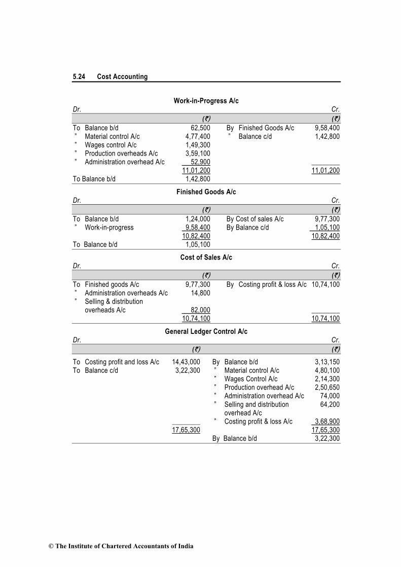
5.24 Cost Accounting
Work-in-Progress A/c Dr. Cr.
(`) (`)
To Balance b/d 62,500 By Finished Goods A/c 9,58,400 ” Material control A/c 4,77,400 ” Balance c/d 1,42,800 ” Wages control A/c 1,49,300 ” Production overheads A/c 3,59,100 ” Administration overhead A/c 52,900 ________
11,01,200 11,01,200 To Balance b/d 1,42,800
Finished Goods A/c Dr. Cr.
(`) (`)
1,24,000 By Cost of sales A/c 9,77,300 9,58,400 By Balance c/d 1,05,100 10,82,400 10,82,400
To Balance b/d ” Work-in-progress
To Balance b/d 1,05,100
Cost of Sales A/c Dr. Cr.
(`) (`)
To Finished goods A/c 9,77,300 By Costing profit & loss A/c 10,74,100 ” Administration overheads A/c 14,800 ” Selling & distribution
overheads A/c 82,000 ________ 10,74,100 10,74,100
General Ledger Control A/c Dr. Cr.
(`) (`)
To Costing profit and loss A/c 14,43,000 By Balance b/d 3,13,150 To Balance c/d 3,22,300 ” Material control A/c 4,80,100
” Wages Control A/c 2,14,300 ” Production overhead A/c 2,50,650 ” Administration overhead A/c 74,000 ” Selling and distribution 64,200
overhead A/c ________ ” Costing profit & loss A/c 3,68,900 17,65,300 17,65,300
By Balance b/d 3,22,300
© The Institute of Chartered Accountants of India

Non-Integrated Accounts 5.25
Costing Profit & Loss A/c
Dr. Cr.
(`) (`)
To Cost of sales A/c 10,74,100 By General ledger control A/c ” General ledger control A/c 3,68,900 (Sales) 14,43,000 (Profit for the period) ________ ________ 14,43,000 14,43,000
Trial Balance as at 30th September, 2012
Dr. Cr. (`) (`) Material control A/c 74,900 Production overhead A/c 6,150 Administration overhead A/c 2,300 Selling and distribution overhead A/c 4,350 Work-in-progress A/c 1,42,800 Finished goods A/c 1,05,100 General ledger control A/c _______ 3,22,300 3,28,950 3,28,950
Illustration 7 (Computation of missing figures)
(a) A fire destroyed some accounting records of a company. You have been able to collect
the following from the spoilt papers/records and as a result of consultation with accounting
staff in respect of January, 2013:
(i) Incomplete Ledger Entries:
Raw Materials A/c
(`) (`)
Beginning Inventory 32,000
Work-in-Progress A/c
(`) (`)
Beginning Inventory 9,200 Finished Stock 1,51,000
Creditors A/c
(`) (`)
Opening Balance 16,400
Closing Balance 19,200
© The Institute of Chartered Accountants of India

5.26 Cost Accounting
Manufacturing Overheads A/c
(`) (`)
Amount Spent 29,600
Finished Goods A/c
(`) (`)
Opening Inventory 24,000
Closing Inventory 30,000
(ii) Additional Information:
(1) The cash-book showed that ` 89,200 have been paid to creditors for raw-material.
(2) Ending inventory of work-in-progress included material ` 5,000 on which 300 direct labour hours have been booked against wages and overheads.
(3) The job card showed that workers have worked for 7,000 hours. The wage rate is ` 10 per labour hour.
(4) Overhead recovery rate was ` 4 per direct labour hour.
You are required to complete the above accounts in the cost ledger of the company:
Solution:
Dr. Creditors A/c Cr.
(`) (`)
To Cash & Bank (1) 89,200 By Balance b/d 16,400
To Balance c/d 19,200 By Purchases (Balancing figure) 92,000
1,08,400 1,08,400
Dr. Work-in-progress A/c Cr.
(`) (`)
To Balance b/d 9,200 By Finished stock 1,51,000
To Raw-materials 53,000 By Balance c/d :
(Balancing figure) Material (2) : ` 5,000
To Wages Control (3) 70,000 Labour (2) : ` 3,000
(7,000 hrs. × ` 10) (300 hrs. × `10)
To Overheads Control (4) 28,000 Overheads (2) : ` 1,200 9,200
(7,000 hrs. × ` 4) _______ (300 hrs. × `4) _______
1,60,200 1,60,200
© The Institute of Chartered Accountants of India

Non-Integrated Accounts 5.27
Dr. Raw-materials A/c Cr.
(`) (`)
To Balance b/d 32,000 By Work-in-progress 53,000 To Purchases 92,000 (As above) (As above) _______ By Balance c/d 71,000 1,24,000 1,24,000
Dr. Finished Goods A/c Cr.
(`) (`)
To Balance b/d 24,000 By Cost of sales 1,45,000 To W.I.P. 1,51,000 (Balancing figure) (As above) _______ By Balance c/d 30,000 1,75,000 1,75,000
Dr. Manufacturing Overheads A/c Cr.
(`) (`)
To Sundries 29,600 By W.I.P. (7000 hrs. × ` 4) 28,000
______ By Under-absorbed Overheads A/c 1,600
29,600 29,600
Illustration 8: (Finding out of missing figures)
The following incomplete accounts are furnished to you for the month ended 31st October,
2012.
Stores Control Account
1.10.12 To Balance ` 54,000
Work in Progress Control Account
1.10.12 To Balance ` 6,000
Finished Goods Control Account
1.10.12 To Balance ` 75,000
Factory Overheads Control Account
Total debits for October, 2012 ` 45,000
Factory Overheads Applied Account
Cost of Goods Sold Account
© The Institute of Chartered Accountants of India

5.28 Cost Accounting
Creditors for Purchases Account
1.10.12 by Balance ` 30,000
Additional information:
(i) The factory overheads are applied by using a budgeted rate based on Direct Labour
Hours. The budget for overheads for 2012 is ` 6,75,000 and the budget of direct labour
hours is 4,50,000.
(ii) The balance in the account of creditors for purchases on 31.10.12 is ` 15,000 and the
payments made to creditors in October, 2012 amount to ` 1,05,000.
(iii) The finished goods inventory as on 31st October, 2012 is ` 66,000.
(iv) The cost of goods sold during the month was ` 1,95,000.
(v) On 31st October, 2012 there was only one unfinished job in the factory. The cost records
show that ` 3,000 (1,200 direct labour hours) of Direct Labour Cost and ` 6,000 of Direct
Material Cost had been charged.
(vi) A total of 28,200 direct labour hours were worked in October, 2012. All factory workers
earn same rate of pay.
(vii) All actual factory overheads incurred in October, 2012 have been posted.
You are required to find:
(a) Materials purchased during October, 2012.
(b) Cost of goods completed in October, 2012.
(c) Overheads applied to production in October, 2012.
(d) Balance of work in progress on 31st October, 2012.
(e) Direct materials consumed during October, 2012.
(f) Balance of Stores Control Account on 31st October, 2012.
(g) Over absorbed or under absorbed overheads for October, 2012.
Solution :
Working Notes :
(i) Overhead recovery rate per direct labour hour :
Budgeted factory overheads : ` 6,75,000
Budgeted direct labour hours : 4,50,000
Overhead recovery rate = hours labourdirect Budgeted
overheadsfactory Budgeted
© The Institute of Chartered Accountants of India

Non-Integrated Accounts 5.29
= `
6,75,000
4,50,000 hours
= ` 1.50 per direct labour
(ii) Direct wage rate per hour :
Direct labour cost of WIP : ` 3,000
(on 31st October 2012)
Direct labour hours of WIP : 1,200 hours
Direct wage rate per hour = Direct labour cost on WIP
Direct labour hours on WIP
= 3,000
1,200 hours
`
= `2.50
(iii) Total direct wages charged to production:
Total direct labour hours spent on production × Direct wage rate per hour
= 28,200 hours × ` 2.50 = ` 70,500
(a) Material purchased during October, 2012
(`)
Payment made to creditors 1,05,000
Add : Closing balance in the account of creditors for purchase 15,000
1,20,000
Less : Opening balance 30,000
Material purchased 90,000
(b) Cost of goods completed in October, 2012
(`)
The cost of goods sold during the month 1,95,000
Add : Closing finished goods inventory 66,000
2,61,000
Less : Opening finished goods inventory 75,000
Cost of goods completed during the month 1,86,000
(c) Overhead applied to production in October, 2012
= 28,200 hours × ` 1.50 = ` 42,300
(d) Balance of Work-in-progress on 31st October, 2012
(`)
Direct material cost 6,000
Direct labour cost 3,000
Overheads (1,200 hours × ` 1.50) 1,800
10,800
© The Institute of Chartered Accountants of India

5.30 Cost Accounting
(e) Direct material consumed during October, 2012 ` 78,000
(Refer to following Account)
Dr. Work in progress Control A/c Cr.
(`) (`)
1.10.12 To Opening Balance 6,000 By Finished goods 1,86,000 ’’ To Direct wages 70,500 (As per (b) above) [Refer to Working Note (iii)] By Balance of WIP 10,800 To Factory Overheads 42,300 (As per (d) above) [As per (c) above] To Balancing figure 78,000 (Material consumed) _______ _______ 1,96,800 1,96,800
(f) Balance of Stores Control Account on 31st October, 2012 ` 66,000
(Refer to following Account)
Dr. Stores Control Account Cr.
(`) (`)
1.10.12 To Balance 54,000 31.10.12 By W.I.P. Control A/c 78,000
To Creditors A/c 90,000 (As per (e) above)
for materials purchased By Balance c/d 66,000
(As per (a) above) _______ (Balancing figure) _______
1,44,000 1,44,000
(g) Over-absorbed or under-absorbed overheads for October, 2012 : Balance in Factory
Overhead Account below showing that ` 2,700 is under-absorbed.
Dr. Factory Overhead Account Cr.
(`) (`)
To General Ledger Adj. A/c 45,000 31.10.12 By Factory overhead applied 42,300
(Total debits for Oct. 2012) [Refer to (c) above]
_____ Balance (Under-absorbed) 2,700
45,000 45,000
5.3 Integrated (or Integral) Accounting System
Integrated Accounts is the name given to a system of accounting, whereby cost and financial
accounts are kept in the same set of books. Obviously, then there will be no separate sets of
books for Costing and Financial records. Integrated accounts provide or meet out fully the
information requirement for Costing as well as for Financial Accounts. For Costing it provides
© The Institute of Chartered Accountants of India

Non-Integrated Accounts 5.31
information useful for ascertaining the Cost of each product, job, process, operation of any
other identifiable activity and for carrying necessary analysis. Integrated accounts provide
relevant information which is necessary for preparing profit and loss account and the balance
sheets as per the requirement of law and also helps in exercising effective control over the
liabilities and assets of its business.
5.3.1 Advantages: The main advantages of Integrated Accounts are as follows:
(a) No need for Reconciliation- The question of reconciling costing profit and financial profit
does not arise, as there is only one figure of profit.
(b) Less efforts- Due to use of one set of books, there is a significant saving in efforts made.
(c) Less Time consuming- No delay is caused in obtaining information as it is provided from
books of original entry.
(d) Economical process- It is economical also as it is based on the concept of “Centralisation
of Accounting function”.
5.3.2 Essential pre-requisites for Integrated Accounts: The essential pre-requisites
for integrated accounts include the following steps:
1. The management’s decision about the extent of integration of the two sets of books.
Some concerns find it useful to integrate up to the stage of primary cost or factory cost
while other prefer full integration of the entire accounting records.
2. A suitable coding system must be made available so as to serve the accounting purposes
of financial and cost accounts.
3. An agreed routine, with regard to the treatment of provision for accruals, prepaid
expenses, other adjustment necessary for preparation of interim accounts.
4. Perfect coordination should exist between the staff responsible for the financial and cost aspects of
the accounts and an efficient processing of accounting documents should be ensured.
Under this system there is no need for a separate cost ledger. Of course, there will be a
number of subsidiary ledgers; in addition to the useful Customers’ Ledger and the Bought
Ledger, there will be: (a) Stores Ledger; (b) Stock Ledger and (c) Job Ledger.
5.3.3 Features of Integrated Accounting System: Following are the main points of
integrated accounting:
(a) Complete analysis of cost and sales are kept.
(b) Complete details of all payments in cash are kept
(c) Complete details of all assets and liabilities are kept and this system does not use a
notional account to represent all impersonal accounts
© The Institute of Chartered Accountants of India
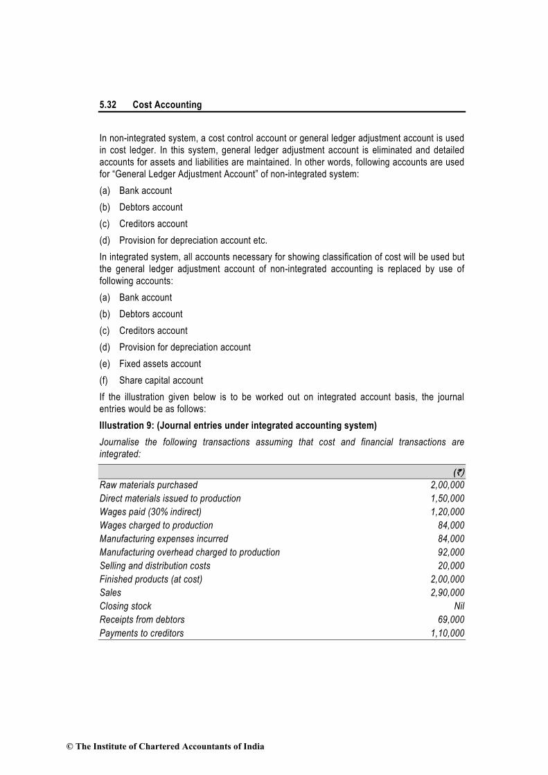
5.32 Cost Accounting
In non-integrated system, a cost control account or general ledger adjustment account is used
in cost ledger. In this system, general ledger adjustment account is eliminated and detailed
accounts for assets and liabilities are maintained. In other words, following accounts are used
for “General Ledger Adjustment Account” of non-integrated system:
(a) Bank account
(b) Debtors account
(c) Creditors account
(d) Provision for depreciation account etc.
In integrated system, all accounts necessary for showing classification of cost will be used but
the general ledger adjustment account of non-integrated accounting is replaced by use of
following accounts:
(a) Bank account
(b) Debtors account
(c) Creditors account
(d) Provision for depreciation account
(e) Fixed assets account
(f) Share capital account
If the illustration given below is to be worked out on integrated account basis, the journal
entries would be as follows:
Illustration 9: (Journal entries under integrated accounting system)
Journalise the following transactions assuming that cost and financial transactions are
integrated:
(`)
Raw materials purchased 2,00,000
Direct materials issued to production 1,50,000
Wages paid (30% indirect) 1,20,000
Wages charged to production 84,000
Manufacturing expenses incurred 84,000
Manufacturing overhead charged to production 92,000
Selling and distribution costs 20,000
Finished products (at cost) 2,00,000
Sales 2,90,000
Closing stock Nil
Receipts from debtors 69,000
Payments to creditors 1,10,000
© The Institute of Chartered Accountants of India
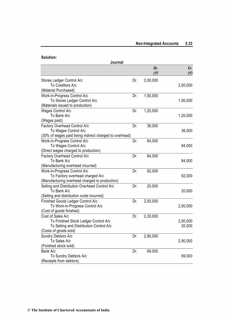
Non-Integrated Accounts 5.33
Solution:
Journal
Dr. Cr.
(`) (`)
Stores Ledger Control A/c Dr. 2,00,000
To Creditors A/c 2,00,000
(Material Purchased)
Work-in-Progress Control A/c Dr. 1,50,000 To Stores Ledger Control A/c 1,50,000 (Materials issued to production)
Wages Control A/c Dr. 1,20,000 To Bank A/c 1,20,000 (Wages paid)
Factory Overhead Control A/c Dr. 36,000 To Wages Control A/c 36,000 (30% of wages paid being indirect charged to overhead)
Work-in-Progress Control A/c Dr. 84,000 To Wages Control A/c 84,000 (Direct wages charged to production)
Factory Overhead Control A/c Dr. 84,000 To Bank A/c 84,000 (Manufacturing overhead incurred)
Work-in-Progress Control A/c Dr. 92,000 To Factory overhead charged A/c 92,000 (Manufacturing overhead charged to production)
Selling and Distribution Overhead Control A/c Dr. 20,000 To Bank A/c 20,000 (Selling and distribution costs incurred)
Finished Goods Ledger Control A/c Dr. 2,00,000 To Work-in-Progress Control A/c 2,00,000 (Cost of goods finished)
Cost of Sales A/c Dr. 2,20,000 To Finished Stock Ledger Control A/c 2,00,000 To Selling and Distribution Control A/c 20,000 (Costs of goods sold)
Sundry Debtors A/c Dr. 2,90,000 To Sales A/c 2,90,000 (Finished stock sold)
Bank A/c Dr. 69,000 To Sundry Debtors A/c 69,000 (Receipts from debtors)
© The Institute of Chartered Accountants of India

5.34 Cost Accounting
Sundry (Creditors) A/c Dr. 1,10,000 To Bank A/c 1,10,000 (Payment made to creditors)
Illustration 10: (Journal entries under integrated accounting system)
Dutta Enterprises operates an integral system of accounting. You are required to pass the Journal
Entries for the following transactions that took place for the year ended 30th June, 2012.
(Narrations are not required.)
(`)
Raw materials purchased (50% on Credit) 6,00,000
Materials issued to production 4,00,000
Wages paid (50% Direct) 2,00,000
Wages charged to production 1,00,000
Factory overheads incurred 80,000
Factory overheads charged to production 1,00,000
Selling and distribution overheads incurred 40,000
Finished goods at cost 5,00,000
Sales (50% Credit) 7,50,000
Closing stock Nil
Receipts from debtors 2,00,000
Payments to creditors 2,00,000
Solution :
Journal Entries under integrated system of accounting for transactions
taking place for the year ended on 30th June, 2012
Dr. Cr.
(`) (`)
Stores Ledger Control A/c Dr.6,00,000
To Sundry Creditors Account 3,00,000
To Cash or Bank Account 3,00,000
Work-in-Progress Control A/c Dr.4,00,000
To Stores Ledger Control A/c 4,00,000
Wages Control A/c Dr.2,00,000
To Cash or Bank Account 2,00,000
Work-in-Progress Control A/c Dr.1,00,000
To Wages Control A/c 1,00,000
Factory Overhead Control A/c Dr.1,00,000
© The Institute of Chartered Accountants of India

Non-Integrated Accounts 5.35
To Wages Control A/c 1,00,000
Factory Overhead Control A/c Dr. 80,000
To Cash or Bank A/c 80,000
Work-in-Progress Control A/c Dr.1,00,000
To Factory Overhead Control A/c 1,00,000
Selling and Distribution Overhead Control A/c Dr. 40,000
To Cash or Bank A/c 40,000
Finished Stock Ledger Control A/c Dr.5,00,000
To Work-in-Progress Control A/c 5,00,000
Cost of Sales A/c Dr.5,40,000
To Finished Stock Ledger Control A/c 5,00,000
To Selling and Distribution Control A/c 40,000
Sundry Debtors Account Dr.3,75,000
Cash or Bank Account Dr.3,75,000
To Sales Account 7,50,000
Cash or Bank A/c Dr.2,00,000
To Sundry Debtors A/c 2,00,000
Sundry Creditors A/c Dr.2,00,000
To Cash or Bank A/c 2,00,000
Illustration 11: (Preparation of ledgers and trial balance under integrated accounting
system)
Bangalore Petrochemicals Co. keeps books on integrated accounting system. The following
balances appear in the books as on 1st January, 2012.
Dr. Cr.
(`) (`)
Stores control A/c 18,000
Work-in-Progress A/c 17,000
Finished goods A/c 13,000
Bank A/c 10,000
Creditors A/c 8,000
Fixed assets A/c 55,000
Debtors A/c 12,000
Share capital A/c 80,000
Depreciation provision A/c 5,000
Profit and loss A/c _______ 32,000
1,25,000 1,25,000
© The Institute of Chartered Accountants of India

5.36 Cost Accounting
Transaction for the year ended 31st Dec., 2012 were as given below:
(`) (`)
Wages-direct 87,000
Wages-indirect 5,000 92,000
Purchase of materials (on credit) 1,00,000
Materials issued to production 1,10,000
Materials for repairs 2,000
Goods finished during the year (at cost) 2,15,000
Sales (credit) 3,00,000
Cost of goods sold 2,20,000
Production overhead absorbed 48,000
Production overhead incurred 40,000
Administration overhead incurred 12,000
Selling overhead incurred 14,000
Payments of creditors 1,01,000
Payments of debtors 2,90,000
Depreciation of machinery 1,300
Prepaid rent (included in factory overheads) 300
Write up accounts in the integrated ledger and prepare a trial balance.
Solution :
Stores Control Account
Dr. Cr.
2012 (`) 2012 (`)
Jan. 1 To Balance b/d 18,000 Dec.31By Work-in-Progress A/c 1,10,000
Dec. 31 ” Creditors A/c 1,00,000 ” Production overheads A/c 2,000
________ ” Balance c/d 6,000
1,18,000 1,18,000
2013
Jan. 1 To Balance b/d 6,000
Wages Control Account
2012 (`) 2012 (`)
Dec. 31 To Bank A/c 92,000 Dec. 31 By Work-in-Progress A/c 87,000
______ ” Production overheads A/c 5,000
92,000 92,000
© The Institute of Chartered Accountants of India
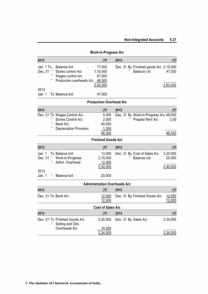
Non-Integrated Accounts 5.37
Work-in-Progress A/c
2012 (`) 2012 (`)
Jan. 1 To Balance b/d 17,000 Dec. 31 By Finished goods A/c 2,15,000
Dec. 31 ” Stores control A/c 1,10,000 ” Balance c/d 47,000
” Wages control A/c 87,000 ” Production overheads A/c 48,000 _______
2,62,000 2,62,000
2013
Jan. 1 To Balance b/d 47,000
Production Overhead A/c
2012 (`) 2012 (`)
Dec. 31 To Wages Control A/c 5,000 Dec. 31 By Work-in-Progress A/c 48,000
” Stores Control A/c 2,000 ” Prepaid Rent A/c 3,00
” Bank A/c 40,000
” Depreciation Provision 1,300 ______
48,300 48,300
Finished Goods A/c
2012 (`) 2012 (`)
Jan. 1 To Balance b/d 13,000 Dec. 31 By Cost of Sales A/c 2,20,000 Dec. 31 ” Work-in-Progress 2,15,000 ” Balance c/d 20,000 ” Admn. Overhead 12,000 _______ 2,40,000 2,40,000 2013 Jan. 1 ” Balance b/d 20,000
Administration Overheads A/c
2012 (`) 2012 (`)
Dec. 31 To Bank A/c 12,000 Dec. 31 By Finished Goods A/c 12,000 12,000 12,000
Cost of Sales A/c
2012 (`) 2012 (`)
Dec. 31 To Finished Goods A/c 2,20,000 Dec. 31 By Sales A/c 2,34,000 ” Selling and Dist. Overheads A/c 14,000 _______ 2,34,000 2,34,000
© The Institute of Chartered Accountants of India
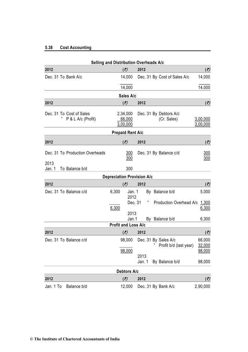
5.38 Cost Accounting
Selling and Distribution Overheads A/c
2012 (`) 2012 (`)
Dec. 31 To Bank A/c 14,000 Dec. 31 By Cost of Sales A/c 14,000 14,000 14,000
Sales A/c
2012 (`) 2012 (`)
Dec. 31 To Cost of Sales 2,34,000 Dec. 31 By Debtors A/c ” P & L A/c (Profit) 66,000 (Cr. Sales) 3,00,000 3,00,000 3,00,000
Prepaid Rent A/c
2012 (`) 2012 (`)
Dec. 31 To Production Overheads 300 Dec. 31 By Balance c/d 300 300 300 2013 Jan. 1 To Balance b/d 300
Depreciation Provision A/c
2012 (`) 2012 (`)
Dec. 31 To Balance c/d 6,300 Jan. 1 By Balance b/d 5,000
2012 _____ Dec. 31 ” Production Overhead A/c 1,300
6,300 6,300
2013
Jan.1 By Balance b/d 6,300
Profit and Loss A/c
2012 (`) 2012 (`)
Dec. 31 To Balance c/d 98,000 Dec. 31 By Sales A/c 66,000
______ ” Profit b/d (last year) 32,000
98,000 98,000
2013
Jan. 1 By Balance b/d 98,000
Debtors A/c
2012 (`) 2012 (`)
Jan. 1 To Balance b/d 12,000 Dec. 31 By Bank A/c 2,90,000
© The Institute of Chartered Accountants of India

Non-Integrated Accounts 5.39
Dec. 31 To Sales 3,00,000 By Balance c/d 22,000
3,12,000 3,12,000
2013
Jan. 1 To Balance b/d 22,000
Creditors A/c
2012 (`) 2012 (`)
Dec. 31 To Bank 1,01,000 Jan. 1 By Balance b/d 8,000
To Balance c/d 7,000 Dec. 31 By Stores Control A/c 1,00,000
1,08,000 1,08,000
2013
Jan. 1 By Balance b/d 7,000
Bank A/c
2012 (`) 2012 (`)
Jan. 1 To Balance b/d 10,000 Dec. 31 By Creditors 1,01,000
Dec. 31 ” Debtors 2,90,000 ” Wages Control A/c 92,000
” Production Overhead A/c 40,000
” Admn. Overhead A/c 12,000
” Selling & Distribution
Overhead A/c 14,000 _______ ” Balance c/d 41,000
3,00,000 3,00,000
2013
Jan. 1 To Balance b/d 41,000
Fixed Assets A/c
2012 (`) 2012 (`)
Jan. 1 To Balance b/d 55,000 Dec. 31 By Balance c/d 55,000
55,000 55,000
2013
Jan. 1 To Balance b/d 55,000
Share Capital A/c
2012 (`) 2012 (`)
Dec. 31 To Balance c/d 80,000 Jan. 1 By Balance b/d 80,000
80,000 80,000
2013
Jan. 1 By Balance b/d 80,000
© The Institute of Chartered Accountants of India

5.40 Cost Accounting
Trial Balance
As on 31st December, 2012
Dr. Cr.
(`) (`)
Stores Control A/c 6,000
Work-in-Progress A/c 47,000
Finished Goods A/c 20,000
Bank A/c 41,000
Creditors A/c 7,000
Fixed Assets A/c 55,000
Debtors A/c 22,000
Share Capital A/c 80,000
Depreciation Provision A/c 6,300
Profit and Loss A/c 98,000
Prepaid Rent A/c 300 _______
1,91,300 1,91,300
Illustration 12: (Preparation of control accounts under non-integrated accounting
system)
A company operates on historic job cost accounting system, which is not integrated with the
financial accounts. At the beginning of a month, the opening balances in cost ledger were:
` (in lakhs)
Stores Ledger Control Account 80
Work-in-Progress Control Account 20
Finished Goods Control Account 430
Building Construction Account 10
Cost Ledger Control Account 540
During the month, the following transaction took place:
Materials − Purchased 40
Issued to production 50
Issued to general maintenance 6
Issued to building construction 4
Wages − Gross wages paid 150
Indirect wages 40
For building construction 10
Works Overheads − Actual amount incurred 160
© The Institute of Chartered Accountants of India

Non-Integrated Accounts 5.41
(excluding items shown above)
Absorbed in building construction 20
Under absorbed 8
Royalty paid 5
Selling, distribution and administration overheads 25
Sales 450
At the end of the month, the stock of raw material and work-in-progress was ` 55 lakhs and
` 25 lakhs respectively. The loss arising in the raw material accounts is treated as factory
overheads. The building under construction was completed during the month. Company’s
gross profit margin is 20% on sales.
Prepare the relevant control accounts to record the above transactions in the cost ledger of
the company.
Solution: Amount (in lakhs)
Dr. Cost Ledger Control A/c Cr.
(`) (`)
To Costing P & L A/c 450 By Balance b/d 540
To Building Const. A/c 44 By Stores Ledger Control A/c 40
To Balance c/d 483 By Wages Control A/c 150
By Works Overhead Control A/c 160
By Royalty A/c 5
By Selling, Distribution and
Administration Overheads A/c 25
___ By Costing Profit & Loss A/c 57
977 977
Dr. Stores Ledger Control A/c Cr.
(`) (`)
To Balance b/d 80 By WIP Control A/c 50
To Cost Ledger Control A/c 40 By Works Overhead Control A/c 6
By Building Const. A/c 4
By Balance c/d 55
By Works Overhead Control A/c 5
___ (Loss) ___
120 120
© The Institute of Chartered Accountants of India

5.42 Cost Accounting
Dr. Work-in-Progress Control A/c Cr.
(`) (`)
To Balance b/d 20 By Finished Goods Control A/c 333
To Stores Ledger Control A/c 50 By Closing Balance 25
To Wage Control A/c 100
To Works Overhead Control A/c 183
To Royalty A/c 5 ___
358 358
Dr. Works Overhead Control A/c Cr.
(`) (`)
To Stores Ledger Control A/c 6 By Building Const. A/c 20
To Wage Control A/c 40 By WIP Control A/c 183
To Cost Ledger Control A/c 160 By Balance (Costing P & L A/c) 8
To Stores Ledger Control A/c (Loss) 5 ___
211 211
Dr. Wages Control A/c Cr.
(`) (`)
To Cost Ledger Control A/c 150 By Works Overhead Control A/c 40 By Building Const. A/c 10 ___ By WIP Control A/c 100 150 150
Dr. Royalty A/c Cr.
(`) (`)
To Cost Ledger Control A/c 5 By WIP Control A/c 5 5 5
Dr. Cost of Goods Sold A/c Cr.
(`) (`)
To Finished Goods Control A/c 360 By Cost of Sales A/c 360
360 360
Dr. Selling, Distribution and Administration Overhead A/c Cr.
(`) (`)
To Cost Ledger Control A/c 25 By Cost of Sales A/c 25
25 25
© The Institute of Chartered Accountants of India

Non-Integrated Accounts 5.43
Dr. Finished Goods Control A/c Cr.
(`) (`)
To Balance b/d 430 By Cost of Goods Sold A/c 360
(450 x 80/100)
To WIP Control A/c 333 By Balance 403
763 763
Dr. Cost of Sales A/c Cr.
(`) (`)
To Cost of Goods Sold A/c 360 By Costing P & L A/c 385
To Selling, distribution and
administration overhead A/c 25 ___
385 385
Dr. Costing P & L A/c Cr.
(`) (`)
To Cost of Sales A/c 385 By Cost Ledger Control A/c 450
To Works Overhead Control A/c 8
To Cost Ledger Control A/c (Profit) 57 ___
450 450
Dr. Building Construction A/c Cr.
(`) (`)
To Balance b/d 10 By Cost Ledger Control A/c 44
To Stores Ledger Control A/c 4
To Wage Control A/c 10
To Works Overhead Control A/c 20 __
44 44
(` in lakhs)
Trial Balance
Dr. Cr.
To Stores Ledger Control A/c 55
To WIP Control A/c 25
To Finished Goods Control A/c 403
To Cost Ledger Adjustment A/c ___ 483
483 483
© The Institute of Chartered Accountants of India

5.44 Cost Accounting
5.4 Reconciliation of Cost and Financial Accounts
When the cost and financial accounts are kept separately, it is imperative that those should be
reconciled, otherwise the cost accounts would not be reliable. In this connection, it is neces-
sary to remember that a reconciliation of the two sets of accounts only can be made if both the
sets contain sufficient details as would enable the causes of differences to be located. It is,
therefore, important that in the financial accounts, the expenses should be analysed in the
same way as in the cost accounts.
In the text book, there appears a General Ledger Adjustment Account as would appear in the
Cost Ledger, students should study the entries therein as well as a discussion that follows to
explain the manner in which the details of items included therein could be reconciled with the
corresponding items appearing in the financial accounts. They would thus realise that the
reconciliation of the balances generally, is possible preparing a Memorandum Reconciliation
Account. In this account, the items charged in one set of accounts but not in the other or those
charged in excess as compared to that in the other are collected and by adding or subtracting
them from the balance of the amount of profit shown by one of the accounts, shown by the
other can be reached. The procedure is similar to the one followed for reconciling the balance
with a bank that shown by the cash book or the ledger.
It is important, however, to know the causes which, generally, give rise to differences in the
Cost and Financial Accounts. These are briefly summarised below :
5.4.1 Items included in the financial accounts but not in cost accounts:
1. Items included in Financial Accounts only-
(a) Purely Financial Expenses :
(i) Interest on loans or bank mortgages.
(ii) Expenses and discounts on issue of shares, debentures etc.
(iii) Other capital losses i.e., loss by fire not covered by insurance etc.
(iv) Losses on the sales of fixed assets and investments
(v) Goodwill written off
(vi) Preliminary expenses written off
(vii) Income tax, donations, subscriptions
(viii) Expenses of the company’s share transfer office, if any.
(b) Purely Financial Income
(i) Interest received on bank deposits, loans and investments
(ii) Dividends received
(iii) Profits on the sale of fixed assets and investments
© The Institute of Chartered Accountants of India

Non-Integrated Accounts 5.45
(iv) Transfer fee received.
(v) Rent receivables
2. Item included in the cost accounts only (notional expenses):
(i) Charges in lieu of rent where premises are owned
(ii) Interest on capital at notional figure though not incurred
(iii) Salary for the proprietor at notional figure though not incurred
(iv) Notional Depreciation on the assets fully depreciated for which book value is nil.
(c) Items whose treatment is different in the two sets of accounts. The objective of cost
accounting is to provide information to management for decision making and control
purposes while financial accounting conforms to external reporting requirements. Hence
there are chances that certain items are treated differently in the two sets of accounts.
For example, LIFO method is not allowed for inventory valuation in India as per the
Accounting Standard 2 issued by the Council of the ICAI. However, this method may be
adopted for cost accounts as it is more suitable for arriving at costs which shall be used
as a base for deciding selling prices. Similarly cost accounting may use a different
method of depreciation than what is allowed under financial accounting.
(d) Varying basis of valuation: It is another factor which sometimes is responsible for the
difference. It is well known that in financial accounts stock are valued either at cost or
market price, whichever is lower. But in Cost Accounts, stocks are only valued at cost.
5.4.2 Procedure for reconciliation : There are 3 steps involved in the procedure for
reconciliation.
1. Ascertainment of profit as per financial accounts
2. Ascertainment of profit as per cost accounts
3. Reconciliation of both the profits (similar to the bank reconciliation statement)
Circumstances where reconciliation statement can be avoided: When the Cost and
Financial Accounts are integrated - there is no need to have a separate reconciliation
statement between the two sets of accounts. Integration means that the same set of accounts
fulfil the requirement of both i.e., Cost and Financial Accounts.
Illustration 13: (Calculation of profit as per financial accounts and as per cost accounts
and reconciliation of profits)
The following figures are available from the financial records of ABC Manufacturing Co. Ltd.
for the year ended 31-3-2013.
(`)
Sales (20,000 units) 25,00,000
Materials 10,00,000
© The Institute of Chartered Accountants of India

5.46 Cost Accounting
Wages 5,00,000
Factory Overheads 4,50,000
Office and administrative Overhead 2,60,000
Selling and distribution Overheads 1,80,000
Finished goods (1,230 units) 1,50,000
(`)
Work-in-Progress :
Materials 30,000
Labour 20,000
Factory overheads 20,000 70,000
Goodwill written off 2,00,000
Interest on capital 20,000
In the Costing records, factory overhead is charged at 100% wages, administration overhead
10% of factory cost and selling and distribution overhead at the rate of ` 10 per unit sold.
Prepare a statement reconciling the profit as per cost records with the profit as per financial records.
Solution :
Profit & Loss Account of ABC Manufacturing Co. Ltd.
(for the year ended 31-3-2013)
(`) (`)
To Opening Stock - By Sales (20,000 units) 25,00,000
To Materials 10,00,000 ” Closing Stock :
To Wages 5,00,000 ” Finished goods (1,230 units) 1,50,000
To Factory Overheads 4,50,000 Work-in-Progress 70,000
To Office & Admn. Overheads 2,60,000
To Selling & Dist. Overheads 1,80,000
To Goodwill written off 2,00,000
To Interest on Capital 20,000
To Profit 1,10,000 ________
27,20,000 27,20,000
Cost Sheet
(`)
Materials 10,00,000
Wages 5,00,000
Direct Expenses Nil
Prime Cost 15,00,000
Add : Factory overhead at 100% wages 5,00,000
© The Institute of Chartered Accountants of India

Non-Integrated Accounts 5.47
20,00,000
Less : Closing WIP (70,000)
Factory Cost of (20,000 + 1,230) units 19,30,000
Office & Admn. Overhead 10% of Factory cost 1,93,000
21,23,000
Less: Closing Stock of finished goods (1,230 units) (1,23,000)*
Production Cost of 20,000 units 20,00,000
Selling & Dist. Overhead @ ` 10 per unit 2,00,000
Cost of sales of 20,000 units 22,00,000
Sales of 20,000 units 25,00,000
Profit 3,00,000
* (` 21,23,000 x 1,230 units/ 21,230 units)
Reconciliation Statement
(`) (`)
Profit as per Cost Accounts 3,00,000
Add : Factory overheads over-absorbed (` 5,00,000 – ` 4,50,000) 50,000
Selling & Dist. Overhead over-absorbed (` 2,00,000 – ` 1,80,000) 20,000
Difference in the valuation of closing stock of
finished goods (` 1,50,000 – ` 1,23,000) 27,000 97,000
3,97,000
Less: Office & Admn. overhead under-absorbed
(` 2,60,000 – ` 1,93,000) 67,000
Goodwill written off taken in financial accounts 2,00,000
Interest on capital 20,000 2,87,000
Profit as per financial accounts 1,10,000
Illustration 14: (Calculation of profit as per financial account and cost account and
reconciliation of profit)
Following are the figures extracted from the Cost Ledger of a manufacturing unit.
(`)
Stores :
Opening balance 15,000
Purchases 80,000
Transfer from WIP 40,000
Issue to WIP 80,000
Issue to repairs and maintenance 10,000
Sold as a special case of cost 5,000
© The Institute of Chartered Accountants of India

5.48 Cost Accounting
Shortage in the year 3,000
Work-in-Progress :
Opening inventory 30,000
Direct labour cost charged 30,000
Overhead cost charged 1,20,000
Closing Balance 20,000
Finished Products :
Entire output is sold at 10% profit on actual cost from work-in-process.
Others :
Wages for the period 35,000
Overhead Expenses 1,25,000
Ascertain the profit or loss as per financial account and cost accounts and reconcile them.
Solution :
Stores Control A/c
Dr. Cr.
(`) (`)
To Balance b/d 15,000 By WIP Control A/c 80,000
” Purchases 80,000 ” Overhead Control A/c 10,000
” WIP Control A/c 40,000 ” General Ledger Adjustment 5,000
” Overhead Control A/c
(Shortages) 3,000
_______ ” Balance c/d 37,000
1,35,000 1,35,000
Wage Control A/c
(`) (`)
To General Ledger Adjustment A/c 35,000 By WIP Control A/c 30,000
______ ” Overhead Control A/c 5,000
35,000 35,000
Overhead Control A/c
(`) (`)
To Material Control A/c 10,000 By WIP Control A/c 1,20,000
” Stores Ledger Control A/c 3,000 By Balance c/d 23,000
” GLA A/c 1,25,000
” Wage Control A/c 5,000 _______
1,43,000 1,43,000
© The Institute of Chartered Accountants of India

Non-Integrated Accounts 5.49
WIP Control A/c
(`) (`)
To Stores Control A/c 80,000 By Stores Control A/c 40,000
” Opening WIP A/c 30,000 ” Closing Balance 20,000
” Wage Control A/c 30,000 ” Finished goods 2,00,000
” Overhead Control A/c 1,20,000 _______
2,60,000 2,60,000
(`)
Finished output at cost 2,00,000
Profit at 10% on actual cost from WIP Sales 20,000
2,20,000
Statement of Profit as per Costing Records
(`)
Direct material Cost 40,000
Direct wages 30,000
Prime Cost 70,000
Production Overheads 1,20,000
Works Cost 1,90,000
Add: Opening WIP 30,000
2,20,000
Less: Closing WIP (20,000)
Cost of finished goods 2,00,000
Profit (10% of cost) 20,000
Sales 2,20,000
Profit & Loss A/c
(`) (`)
To Material (Op. bal. + By Sale 2,20,000
Purchases - Sale) 90,000 ” Closing W-I-P 20,000
” WIP 30,000 ” Closing stores 37,000
” Wages 35,000 ” Net loss 3,000
” Overhead 1,25,000 _______
2,80,000 2,80,000
Reconciliation Statement
(`)
Profit (loss) as per Financial Accounts (3,000)
© The Institute of Chartered Accountants of India

5.50 Cost Accounting
Add: Overheads over absorbed in Cost A/c 23,000
Net Profit as per Accounts 20,000
Illustration15: (Reconciliation of profit)
The following figures, have been extracted from the Financial Accounts of a Manufacturing
Firm for the first year of its operation:
(`)
Direct Material Consumption 50,00,000
Direct Wages 30,00,000
Factory Overhead 16,00,000
Administration Overheads 7,00,000
Selling and Distribution Overheads 9,60,000
Bad Debts 80,000
Preliminary Expenses written off 40,000
Legal Charges 10,000
Dividends Received 1,00,000
Interest Received on Deposits 20,000
Sales (1,20,000 units) 1,20,00,000
Closing Stock :
Finished Goods (4,000 units) 3,20,000
Work-in-Progress 2,40,000
The cost accounts for the same period reveal that the direct material consumption was
` 56,00,000. Factory overhead is recovered at 20% on prime cost. Administration overhead is
recovered at ` 6 per unit of production. Selling and distribution overheads are recovered at
` 8 per unit sold.
Prepare the Profit and Loss Accounts both as per financial records and as per cost records.
Reconcile the profits as per the two records.
Solution:
Profit and Loss Account
(As per financial records)
(`) (`)
To Direct Material 50,00,000 By Sales (1,20,000 units) 1,20,00,000
To Direct Wages 30,00,000 By Closing Stock
To Factory Overheads 16,00,000 WIP 2,40,000
” Gross Profit 29,60,000 Finished Goods (4,000 units) 3,20,000
1,25,60,000 1,25,60,000
To Administration Overheads 7,00,000 By Gross Profit b/d 29,60,000
” Selling and Distribution ” Dividend 1,00,000
Overheads 9,60,000 ” Interest 20,000
© The Institute of Chartered Accountants of India

Non-Integrated Accounts 5.51
” Bad Debts 80,000
” Preliminary Expenses written off 40,000
” Legal Charge 10,000
” Net Profit 12,90,000 ________
30,80,000 30,80,000
Statement of Cost and Profit
(As per Cost Records)
Total
(`)
Direct Material 56,00,000
Direct Wages 30,00,000
Prime Cost 86,00,000
Factory Overhead 17,20,000
1,03,20,000
Less: Closing Stock (WIP) (2,40,000)
Works Cost (1,24,000 units) 1,00,80,000
Administration overhead (1,24,000 units @ ` 6 p.u.) 7,44,000
Cost of production of (1,24,000 units) 1,08,24,000
Less: Finished Goods (4,000 units @ ` 87.29) (3,49,160)
Cost of goods sold (1,20,000 units) 1,04,74,840
Selling and Distribution Overhead (1,20,000 @ ` 8 p.u.) 9,60,000
Cost of Sales 1,14,34,840
Net profit (Balancing figure) 5,65,160
Sales Revenue 1,20,00,000
Statement of Reconciliation of profit as obtained under Cost and Financial Accounts
(`) (`)
Profit as per Cost Records 5,65,160
Add: Excess of Material Consumption 6,00,000
“ Factory Overhead 1,20,000
“ Administration Overhead 44,000
Dividend Received 1,00,000
Interest Received 20,000 8,84,000
14,49,160
Less: Bad debts 80,000
Preliminary expenses written off 40,000
Legal Charges 10,000
Over-valuation of stock in cost book (`3,49,160 – `3,20,000) 29,160 (1,59,160)
Profit as per Financial Records 12,90,000
© The Institute of Chartered Accountants of India

5.52 Cost Accounting
Illustration 16: (Calculation of profit and profit reconciliation)
The following information is available from the financial books of a company having a normal
production capacity of 60,000 units for the year ended 31st March, 2013:
(i) Sales ` 10,00,000 (50,000 units).
(ii) There was no opening and closing stock of finished units.
(iii) Direct material and direct wages cost were ` 5,00,000 and ` 2,50,000 respectively.
(iv) Actual factory expenses were ` 1,50,000 of which 60% are fixed.
(v) Actual administrative expenses were ` 45,000 which are completely fixed.
(vi) Actual selling and distribution expenses were ` 30,000 of which 40% are fixed.
(vii) Interest and dividends received ` 15,000.
You are required to:
(a) Find out profit as per financial books for the year ended 31st March,2013;
(b) Prepare the cost sheet and ascertain the profit as per cost accounts for the year ended
31st March, 2013 assuming that the indirect expenses are absorbed on the basis of
normal production capacity; and
(c) Prepare a statement reconciling profits shown by financial and cost books.
Solution:
Working Note:
Profit & Loss Account
(for the year ended 31st March, 2013)
(`) (`)
To Direct material 5,00,000 By Sales 50,000 units 10,00,000
To Direct wages 2,50,000 By Interest and dividends 15,000
To Actual factory expenses 1,50,000
To Actual administrative expenses 45,000
To Actual selling and distribution
expenses 30,000
To Profit 40,000 _______
10,15,000 10,15,000
(a) Profit as per financial books for the year ended 31st March, 2013 is ` 40,000 (Refer to
above Working note).
© The Institute of Chartered Accountants of India

Non-Integrated Accounts 5.53
(b) Cost Sheet
(for the year ended 31st March, 2013)
(`)
Direct material 5,00,000
Direct wages 2,50,000
Prime cost 7,50,000
Factory expenses:
Variable : ` 60,000
Fixed : (`90,000 x 50,000/60,000) ` 75,000 1,35,000
Works cost 8,85,000
Administrative expenses: (`45,000 x 50,000/60,000) 37,500
Cost of production 9,22,500
Selling & distribution expenses:
Variable : ` 18,000
Fixed : ` 10,000 (`12,000 x 50,000/60,000) 28,000
Cost of Sales 9,50,500
Profit 49,500
Sales revenue 10,00,000
(c) Statement of Reconciliation
(Reconciling profit shown by Financial and Cost Accounts)
(`) (`)
Profit as per Cost Account 49,500 −
Add : Income from interest and dividends 15,000 64,500
Less: Factory expenses under-charged in Cost Accounts 15,000
(` 1,50,000 – ` 1,35,000)
Administrative expenses under-charged in Cost Accounts 7,500
(` 45,000 – ` 37,500)
Selling & distribution expenses under—charged in Cost Accounts 2,000 24,500
(` 30,000 – ` 28,000)
Profit as per Financial Accounts 40,000
Illustration 17: (Preparation of memorandum reconciliation account)
M/s. H.K. Piano Company showed a net loss of ` 4,16,000 as per their financial accounts for
the year ended 31st March, 2013. The cost accounts, however, disclosed a net loss of
` 3,28,000 for the same period. The following information was revealed as a result of scrutiny
of the figures of both the sets of books:
(`)
(i) Factory overheads under-recovered 6,000
(ii) Administration overheads over-recovered 4,000
(iii) Depreciation charged in financial accounts 1,20,000
© The Institute of Chartered Accountants of India

5.54 Cost Accounting
(iv) Depreciation recovered in costs 1,30,000
(v) Interest on investment not included in costs 20,000
(vi) Income-tax provided 1,20,000
(vii) Transfer fees (credit in financial books) 2,000
(viii) Stores adjustment (credit in financial books) 2,000
Prepare a Memorandum reconciliation account.
Solution:
Memorandum Reconciliation Account
Dr. Cr.
Particulars (`) Particulars (`)
To Net loss as per costing books 3,28,000 By Administration overhead
To Factory overheads over-recovered in costs 4,000
under-recovered in costs 6,000 By Interest on investments
To Income-tax not provided in costs 1,20,000 not included in costs 20,000
By Depreciation overcharged
in costs 10,000
By Transfer fees in financial books 2,000
By Stores adjustment 2,000
By Net loss as per financial
_______ books 4,16,000
4,54,000 4,54,000
5.5 Summary
• Cost Control Accounts: These are accounts maintained for the purpose of exercising
control over the costing ledgers and also to complete the double entry in cost accounts.
• Integral System of Accounting: A system of accounting where both costing and
financial transactions are recorded in the same set of books.
• Non- Integral System of Accounting: A system of accounting where two sets of books
are maintained- (i) for costing transactions; and (ii) for financial transactions
• Reconciliation: In the Non-Integral System of Accounting, since the cost and financial
accounts are kept separately, it is imperative that those should be reconciled, otherwise
the cost accounts would not be reliable. The reason for differences in the cost & financial
accounts can be of purely financial nature( Income and expenses) and notional nature.
© The Institute of Chartered Accountants of India

6 Job Costing & Batch Costing
Learning Objectives
When you have finished studying this chapter, you should be able to
• Understand the meaning and distinctive features of Job and Batch Costing.
• Understand the accounting procedures to be applied in Job Costing and Batch
Costing.
6.1 Methods of Costing
Today business and industry needs costing systems to meet their individual requirements.
Costing experts believe that it may not be possible to devise a single costing system to fulfill
everybody’s needs. They have developed different methods of costing for different industries
depending upon the type of manufacture and their nature. Mainly the industries can be
grouped into two basic types i.e. Industries doing job work and Industries engaged in mass
production of a single product or identical production.
6.1.1 For industry doing job work: A concern engaged in the execution of specification
order is characterised as a firm producing several items distinguishable from one another by
respective specifications and other details. Such a concern is thought of involved in
performing job works. Production under job work is strictly according to customer’s
specifications and each lot, job or production order is unique. Examples of jobs order type of
production are: ships building, roads, bridges, manufacture of heavy electrical machinery, ma-
chine tools, iron foundries, wood working shops, etc. Here each job or unit of production is
treated as a separate identity for the purpose of costing. The methods of costing and for
ascertaining cost of each job are known as a job costing, contract costing and Batch costing.
6.1.2 For continuous and process type of industries: The continuous or process type
of industry is characterised by the continuous production of uniform products according to
standard specifications. In such a case the successive lots are generally indistinguishable as
to size and form and, even if there is some variation in specifications, it is of a minor
character. Examples of continuous type of industries are chemical and pharmaceutical
products, paper/food products, canning, paints, and varnish oil, rubber, textile etc. Here the
© The Institute of Chartered Accountants of India

6.2 Cost Accounting
methods of Costing used for the purpose of ascertaining costs are: process costing; single
costing; operating costing etc.
6.2 Job Costing
6.2.1 Meaning of Job Costing: CIMA London defines Job Costing as “the category of
basic costing methods which is applicable where the work consists of separate contracts, jobs
or batches each of which is authorised by specific order or contract.” According to this method
costs are collected and accumulated according to jobs, contracts, products or work orders.
Each job or unit of production is treated as a separate entity for the purpose of costing. Job
costing is carried out for the purpose of ascertaining cost of each job and takes into account
the cost of materials, labour and overhead etc. The job costing method is also applicable to
industries in which production is in batches since batch production basically is of the same
character as the job order production, the difference being mainly one in the size of different
orders. The method then may also be described as “Batch Costing”.
6.2.2 Principles of Job Costing: The job costing method of costing may be regarded as the
principal method of costing since the basic object and purpose of all costing
Analysis and ascertain cost of each unit of production
Control and regulate cost
Determine the profitability
The basic principles enunciated for the job costing method are valid essentially for all types of
industry. For example, printing; furniture; hardware; ship-building; heavy machinery; interior
decoration, repairs and other similar work.
6.2.3 Process of Job costing
Prepare a separate cost sheet for each job
Disclose cost of materials issued for the job
Labour charges incurred(on the basis of bill of material and time cards respectively)
When job is completed, overhead charges are added for ascertaining total expenditure
6.2.4 Suitability of Job Costing
When jobs are executed for different customers according to their specifications.
When no two orders are alike and each order/job needs special treatment.
Where the work-in-progress differs from period to period on the basis of the number of
jobs in hand.
© The Institute of Chartered Accountants of India

Job Costing and Batch Costing 6.3
6.2.5 Format of Job Cost Sheet:
JOB COST SHEET
Description :_______________________
Blue Print No.:______________________
Material No.:_______________________
Reference No.:______________________
Job No.:________________________
Quantity:_______________________
Date of delivery:__________________
Date commenced:_________________
Date finished:_____________________
Date Reference Details Material Labour Overhead
Total
Summary of costs Estimated (`) Actual (`)
For the job __________________
Units produced ______________
Cost/unit ___________________
Remarks ____________________
Prepared by : ________________
Checked by: _________________
Direct material cost
Direct wages
Production overhead
PRODUCTION COST
Admn. Selling & Distrn. Ovds.
TOTAL COST
PROFIT/LOSS
SELLING PRICE
6.2.6 Difference between Job Costing and Process Costing: The main points which
distinguish job costing and process costing are as below:
Job Costing Process Costing
(i) A Job is carried out or a product is The process of producing the product has a continuous flow and the product produced is
© The Institute of Chartered Accountants of India

6.4 Cost Accounting
produced by specific orders. homogeneous.
(ii) Costs are determined for each job. Costs are compiled on time basis i.e., for production of a given accounting period for each process or department.
(iii) Each job is separate and independent of other jobs.
Products lose their individual identity as they are manufactured in a continuous flow.
(iv) Each job or order has a number and costs are collected against the same job number.
The unit cost of process is an average cost for the period.
(v) Costs are computed when a job is completed. The cost of a job may be determined by adding all costs against the job.
Costs are calculated at the end of the cost period. The unit cost of a process may be computed by dividing the total cost for the period by the output of the process during that period.
(vi) As production is not continuous and each job may be different, so more managerial attention is required for effective control.
Process of production is usually standardized and is therefore, quite stable. Hence control here is comparatively easier.
6.3 Procedure of job Cost Accounting
Accounting for Materials: An essential requirement of job cost accounting is that direct
materials and their cost must be traced to and identified with specific job or work order. This
segregation of materials cost by jobs or work order is brought about by the use of separate
stores requisitions for each job or work order. Where a bill of material is prepared, it provides
the basis for the preparation of these stores requisitions. But when the entire quantity of
materials specified in the bill of materials is drawn in one lot or in installments, the bill itself
could be made to serve as a substitute for the stores requisition.
After the materials have been issued and the stores requisitions have been priced, it is usual
to enter the value of the stores requisition in a material abstract or analysis book. It serves to
analyse and collect the cost of all direct materials according to job or work orders and
departmental standing orders or expense code numbers. From the abstract book, the
summary of materials cost of each job is posted to individual job cost sheets or cards in the
Work-in-Progress ledger. The postings are usually made weekly or monthly. Similarly, at
periodical intervals, from the material abstract books, summary cost of indirect material is
posted to different standing orders or expense code numbers in the Overhead Expenses
ledger. If any special material has been purchased for a particular job, it is generally the
practice to charge such special material direct to the job concerned without passing it through
the Stores Ledger, as soon as it is purchased.
© The Institute of Chartered Accountants of India

Job Costing and Batch Costing 6.5
If any surplus material is left over in the case of any job, unless it can be immediately and
economically used on some other job, the same is returned to the store room with a proper
supporting document/stores Debit Note or Shop Credit, and the relevant job account is
credited with the value of excess material returned to the store room. If the surplus material is
utilised on some other job, instead of being returned to the store room first, a material transfer
note is prepared. The transfer note would show the number of the transfer to job as well as
transferee job (or jobs) so that, on that basis, the cost thereof can be adjusted in the Work-in-
Progress Ledger.
Accounting for Labour: All direct labour cost must be analysed according to individual jobs
or work orders. Similarly, different types of indirect labour cost also must be collected and
accumulated under appropriate standing order or expenses code number. The analysis of
labour according to jobs or work orders is, usually, made by means of job time cards or
sheets. All direct labour is booked against specific jobs in the job time cards or sheets. All the
idle time also is booked against appropriate standing order expense code number either in the
job time card for each job or on a separate idle time card for each worker (where the job time
card is issued job-wise). The time booked or recorded in the job time and idle time cards is
valued at appropriate rates and entered in the labour abstract or analysis book. All direct
labour cost is accumulated under relevant job or work order numbers, and the total or the
periodical total of each job or work order is then posted to the appropriate job cost card or
sheet in Work-in-Progress ledger. The postings are usually made at the end of each week or
month.
The abstraction of idle time costs under suitable standing order or expenses code numbers is
likewise done and the amounts are posted to the relevant departmental standing order or
expense code number in the Overhead Expenses Ledger at periodical intervals. As regards
other items of indirect labour cost these are collected from the payrolls books for the purpose
of posting against standing order or expenses code numbers in the Overhead Expenses
ledger.
Accounting for Overhead: Manufacturing overheads are collected under suitable standing
order numbers and selling and distribution overheads against cost accounts numbers. Total
overhead expenses so collected are apportioned to service and production departments on
some suitable basis. The expenses of service departments are finally transferred to production
departments. The total overhead of production departments is then applied to products on
some realistic basis, e.g. machine hour; labour hour; percentage of direct wages; percentage
of direct materials; etc. It should be remembered that the use of different methods will lead to
a different amounts being computed for the works overhead charged to a job hence to
different total cost. The problem of accurately absorbing, in each individual job or work order,
the overhead cost of different cost centres or departments involved in the manufacture is
difficult under the job costing method. It is because the cost or the expenses thereof cannot be
© The Institute of Chartered Accountants of India

6.6 Cost Accounting
traced to or identified with any particular job or work order. In such circumstances, the best
that can be done is to apply a suitable overhead rate to each individual article manufactured or
to each production order. This is essentially an arbitrary method.
Price of a job: Price of a job may be arrived by adding the desired percentage of profit to the total
cost of the job.
Treatment of spoiled and defective work: Spoiled work is the quantity of production that has
been totally rejected and cannot be rectified.
Defective work refers to production that is not as perfect as the saleable product but is
capable of being rectified and brought to the required degree of perfection provided some
additional expenditure is incurred. Normally, all the manufacturing operations are not fully
successful; they result in turning out a certain amount of defective work. Nonetheless, over a
period of time it is possible to work out a normal rate of defectives for each manufacturing
process which would represent the number of defective articles which a process shall produce
in spite of due care. Defects arise in the following circumstances:
Circumstances Treatment
(1) Where a percentage of
defective work is allowed
in a particular batch as it
cannot be avoided.
When a normal rate of defectives has already been
established, if the actual number of defectives is within
the normal limit or is near thereto the cost of
rectification will be charged to the whole job and spread
over the entire output of the batch. If, on the other
hand, the number of defective units substantially
exceeds the normal, the cost of rectification of the
number which exceeds the normal will be written off as
a loss in the Costing Profit and Loss Account.
(2) Where defect is due to
bad workmanship.
In this case cost of rectification will be abnormal cost,
i.e., not a legitimate element of the cost. Therefore, the
cost of rectification shall be written off as a loss, unless
by an arrangement, it is to be recovered as a penalty
from the workman concerned. It is possible, however
that the management did provide for a certain
proportion of defectives on account of bad
workmanship as an unavoidable feature of production.
If that be the case, the cost of rectifying to the extent
provided for by the management will be treated as a
normal cost and charged to the batch.
(3) Where defect is due to
the Inspection
Department wrongly
In this case the cost of rectification will be charged to
the department and will not be considered as cost of
manufacture of the batch. Being an abnormal cost, it
© The Institute of Chartered Accountants of India

Job Costing and Batch Costing 6.7
accepting incoming
material of poor quality.
will be written off to the Costing Profit and Loss
Account.
6.3.1 Entries in Control Accounts
1. For purchase of materials-
Stores Ledger Control A/c Dr.
To Cost Ledger Control A/c*
2. For the value of direct materials issued to jobs-
Work-in-Progress Control A/c Dr.
To Stores Ledger Control A/c
3. For return of direct materials from jobs-
Stores Ledger Control A/c Dr.
To Work-in-Progress Control A/c
4. For return of materials to suppliers –
Cost Ledger Control A/c Dr.
To Stores Ledger Control A/c
5. For indirect materials-
Factory Overhead Control A/c Dr.
To Stores Ledger Control A/c
6. For wages paid-
Wages Control A/c Dr.
To Cost Ledger Control A/c
7. For direct wages incurred on jobs-
Work-in-Progress Control A/c Dr.
To Wages Control A/c
8. For indirect wages –
Factory Overhead Control A/c Dr.
To Wages Control A/c
9. For any indirect expense paid-
Factory Overhead Control A/c Dr.
To Cost Ledger Control A/c
10. For charging overhead to jobs-
Work-in-Progress Control A/c Dr.
© The Institute of Chartered Accountants of India

6.8 Cost Accounting
To Factory Overhead Control A/c
11. For the total cost of jobs completed-
Cost of Sales A/c Dr.
To Work-in-Progress Control A/c
12. The balance of Cost of Sales A/c is transferred to Costing Profit and Loss a/c; For such transfer –
Costing Profit and Loss A/c Dr.
To Cost of Sales A/c
13. For the sales value of jobs completed -
Cost Ledger Control A/c Dr.
To Costing Profit and Loss A/c**
*General ledger adjustment account is the other name of Cost Ledger Control Account.
**The balance of Costing Profit and Loss Account shall now represent profit or loss. The balance
of Cost Ledger Control Account shall be carried forwarded. With the balance on all the accounts
trial balance can be drawn.
Illustration 1 (Journal entries in Cost Accounting)
The manufacturing cost of a work order is ` 1,000; 8% of the production against that order
spoiled and the rejection is estimated to have a realisable value of ` 20 only. The normal rate
of spoilage is 2%. Record this in the costing journal.
Solution:
Actual loss due to spoilage = 8% of ` 1,000 = `80 and Normal loss = 2% of ` 1,000 = ` 20,
therefore abnormal loss = ` 60.
The rejection has a realisable value of ` 20, which is to be apportioned between normal loss
and abnormal loss in the ratio of 2 : 6.
The accounting entries necessary for recording the above facts would be :
(`) (`)
Material Control Account Dr. 20
Overhead Control Account Dr. 15
Costing Profit and Loss Control Account Dr. 45
To Work-in-Progress Control Account 80
In the case of defectives being inherent in the manufacturing process, the rectification cost
may be charged to the specific jobs in which they have arisen. In case detectives cannot be
identified with jobs, the cost of rectification may be treated as factory overheads. Abnormal
defectives should be written off to the Costing Profit and Loss Account.
© The Institute of Chartered Accountants of India

Job Costing and Batch Costing 6.9
Illustration 2 (Preparation of job cost sheet)
A shop floor supervisor of a small factory presented the following cost for Job No. 303, to
determine the selling price.
Per Unit (`) Materials 70 Direct wages 18 hours @ ` 2.50 45 (Deptt. X 8 hours ; Deptt. Y 6 hours; Deptt. Z 4 hours) Chargeable expenses 5 120 Add : 33-1/3 % for expenses cost 40
160
Analysis of the Profit/Loss Account
(for the year 2012)
(`) (`)
Materials used 1,50,000 Sales less returns 2,50,000
Direct wages:
Deptt. X 10,000
Deptt. Y 12,000 Deptt. Z 8,000 30,000
Special stores items 4,000
Overheads:
Deptt. X 5,000
Deptt. Y 9,000 Deptt. Z 2,000 16,000
Works cost 2,00,000
Gross profit c/d 50,000 _______
2,50,000 2,50,000
Selling expenses 20,000 Gross profit b/d 50,000
Net profit 30,000 ______
50,000 50,000
It is also noted that average hourly rates for the three Departments X, Y and Z are similar.
You are required to:
Draw up a job cost sheet.
Calculate the entire revised cost using 2012 actual figures as basis.
Add 20% to total cost to determine selling price.
© The Institute of Chartered Accountants of India

6.10 Cost Accounting
Solution:
Job Cost Sheet
Customer Details ——— Job No._________________
Date of commencement —— Date of completion _________
Particulars Amount
(`)
Direct materials 70
Direct wages :
Deptt. X ` 2.50 × 8 hrs. = ` 20.00
Deptt. Y ` 2.50 × 6 hrs. = ` 15.00 Deptt. Z ` 2.50 × 4 hrs. = ` 10.00 45
Chargeable expenses 5
Prime cost 120
Overheads:
Deptt. X = `
`
5,000
10,000× 100 = 50% of ` 20 = ` 10.00
Deptt. Y = `
`
9,000
12,000× 100 = 75% of ` 15 = ` 11.25
Deptt. Z = `
`
2,000
8,000× 100 = 25% of ` 10 = ` 2.50 23.75
Works cost 143.75
Selling expenses = `
`
20,000
2,00,000× 100 = 10% of work cost 14.38
Total cost 158.13
Profit (20% of total cost) 31.63
Selling price 189.76
Illustration 3 (Preparation of factory cost statement and Invoice price of Job)
In a factory following the Job Costing Method, an abstract from the work-in-progress as on 30th September was prepared as under.
Job No. Materials (`) Direct hrs. Labour (`) Factory Overheads applied (`)
115 1325 400 hrs. 800 640
118 810 250 hrs. 500 400
120 765 300 hrs. 475 380
2,900 1,775 1,420
© The Institute of Chartered Accountants of India

Job Costing and Batch Costing 6.11
Materials used in October were as follows:
Materials Requisition No. Job No. Cost (`)
54 118 300
55 118 425
56 118 515
57 120 665
58 121 910
59 124 720
3,535
A summary for labour hours deployed during October is as under:
Job No. Number of Hours
Shop A Shop B
115 25 25
118 90 30
120 75 10
121 65 --
124 25 10
275 75
Indirect Labour: Waiting of material 20 10
Machine breakdown 10 5
Idle time 5 6
Overtime premium 6 5
316 101
A shop credit slip was issued in October, that material issued under Requisition No. 54 was returned back to stores as being not suitable. A material transfer note issued in October indicated that material issued under Requisition No. 55 for Job 118 was directed to Job 124.
The hourly rate in shop A per labour hour is ` 3 per hour while at shop B, it is ` 2 per hour. The factory overhead is applied at the same rate as in September. Job 115, 118 and 120 were completed in October.
You are asked to compute the factory cost of the completed jobs. It is the practice of the management to put a 10% on the factory cost to cover administration and selling overheads and invoice the job to the customer on a total cost plus 20% basis. What would be the invoice price of these three jobs?
© The Institute of Chartered Accountants of India

6.12 Cost Accounting
Solution:
Factory Cost Statement of Completed Job.
Month Job No. Materials Direct labour
Factory overheads (80% of direct labour cost)
Factory cost
(`) (`) (`) (`) (`)
September 115 1,325 800 640 2765
October 115 -- 125 100 225
Total 1,325 925 740 2,990
September 118 810 500 400 1,710
October 118 515 330 264 1,109
Total 1,325 830 664 2,819
September 120 765 475 380 1,620
October 120 665 245 196 1,106
Total 1,430 720 576 2,726
Invoice Price of Complete Job
Job No. 115
(`)
118
(`)
120
(`)
Factory cost 2,990.00 2,819.00 2,726.00
Administration and selling overheads @ 10% of factory cost
299.00
281.90
272.60
Total cost 3,289.00 3,100.90 2,998.60
Profit (20% of total cost) 657.80 620.18 599.72
Invoice Price 3,946.80 3,721.08 3,598.32
Assumption: - Indirect labour costs have been included in the factory overhead which has been recovered as 80% of the labour cost.
6.3.2 Advantages and Disadvantages of Job Costing
Some of the advantages and disadvantages of Job costing are summarised as below:
Advantages Disadvantages
1. The details of Cost of material, labour and overhead for all job is available to control.
1. Job Costing is costly and laborious method.
2. Profitability of each job can be derived. 2. As lot of clerical process is involved the
© The Institute of Chartered Accountants of India

Job Costing and Batch Costing 6.13
chances of error is more.
3. It facilitates production planning. 3. This method is not suitable in inflationary condition.
4. Budgetary control and Standard Costing can be applied in job costing.
4. Previous records of costs will be meaningless if there is any change in market condition.
5. Spoilage and detective can be identified and responsibilities can be fixed accordingly.
6.4 Batch Costing
6.4.1 Meaning of Batch Costing: In batch costing articles are produced in a lot i.e. one
unit of product is not produced but a lot of ‘say’ 500 or 1000 units of such product is produced.
This is a form of job costing. Under job costing, executed job is used as a cost unit, whereas
under batch costing, a lot of similar units which comprises the batch may be used as a cost
unit for ascertaining cost. In the case of batch costing separate cost sheets are maintained for
each batch of products by assigning a batch number. Cost per unit in a batch is ascertained by
dividing the total cost of a batch by number of items produced in that batch. In batch costing
Material cost, direct labour engaged in batch wise and overhead are also recovered in
batchwise. Such a method of Costing is used in the case of pharmaceutical or drug industries,
ready-made garments, industries manufacturing electronic parts of T.V., radio sets etc
Cost per unit in a batch= Total cost of a batch/Number of item produced.
Illustration 4 (Calculation of cost and profit per piece of each batch)
A jobbing factory has undertaken to supply 200 pieces of a component per month for the
ensuing six months. Every month a batch order is opened against which materials and labour
hours are booked at actual. Overheads are levied at a rate per labour hour. The selling price
contracted for is ` 8 per piece. From the following data present the cost and profit per piece of
each batch order and overall position of the order for 1,200 pieces.
Month Batch Material Direct Direct
Output cost wages labour hours
(`) (`)
January 210 650 120 240
February 200 640 140 280
March 220 680 150 280
April 180 630 140 270
May 200 700 150 300
June 220 720 160 320
© The Institute of Chartered Accountants of India

6.14 Cost Accounting
The other details are:
Month Chargeable expenses Direct labour
(`) hours
January 12,000 4,800
February 10,560 4,400
March 12,000 5,000
April 10,580 4,600
May 13,000 5,000
June 12,000 4,800
Solution:
Jan. Feb. March April May June Total
Batch output (in units) 210 200 220 180 200 220 1,230
Sale value ` 1,680 1,600 1,760 1,440 1,600 1,760 9,840
Material cost ` 650 640 680 630 700 720 4,020
Direct wages ` 120 140 150 140 150 160 860
Chargeable expenses* ` 600 672 672 621 780 800 4,145
Total cost ` 1,370 1,452 1,502 1,391 1,630 1,680 9,025
Profit per batch ` 310 148 258 49 –30 80 815
Total cost per unit ` 6.52 7.26 6.83 7.73 8.15 7.64 7.34
Profit per unit ` 1.48 0.74 1.17 0.27 –0.15 0.36 0.66
Overall position of the order for 1,200 units
Sales value of 1,200 units @ ` 8 per unit ` 9,600
Total cost of 1,200 units @ ` 7.34 per unit ` 8,808
Profit ` 792
*
Chargeable expensesDirect labour hours for batch
Direct labour hour for the month×
Illustration 5 (Preparation of Statement of Cost under batch costing)
Rio Limited undertakes to supply 1000 units of a component per month for the months of
January, February and March 2013. Every month a batch order is opened against which
materials and labour cost are booked at actual. Overheads are levied at a rate per labour
hour. The selling price is contracted at ` 15 per unit.
From the following data, present the profit per unit of each batch order and the overall position of the order for the 3000 units.
© The Institute of Chartered Accountants of India
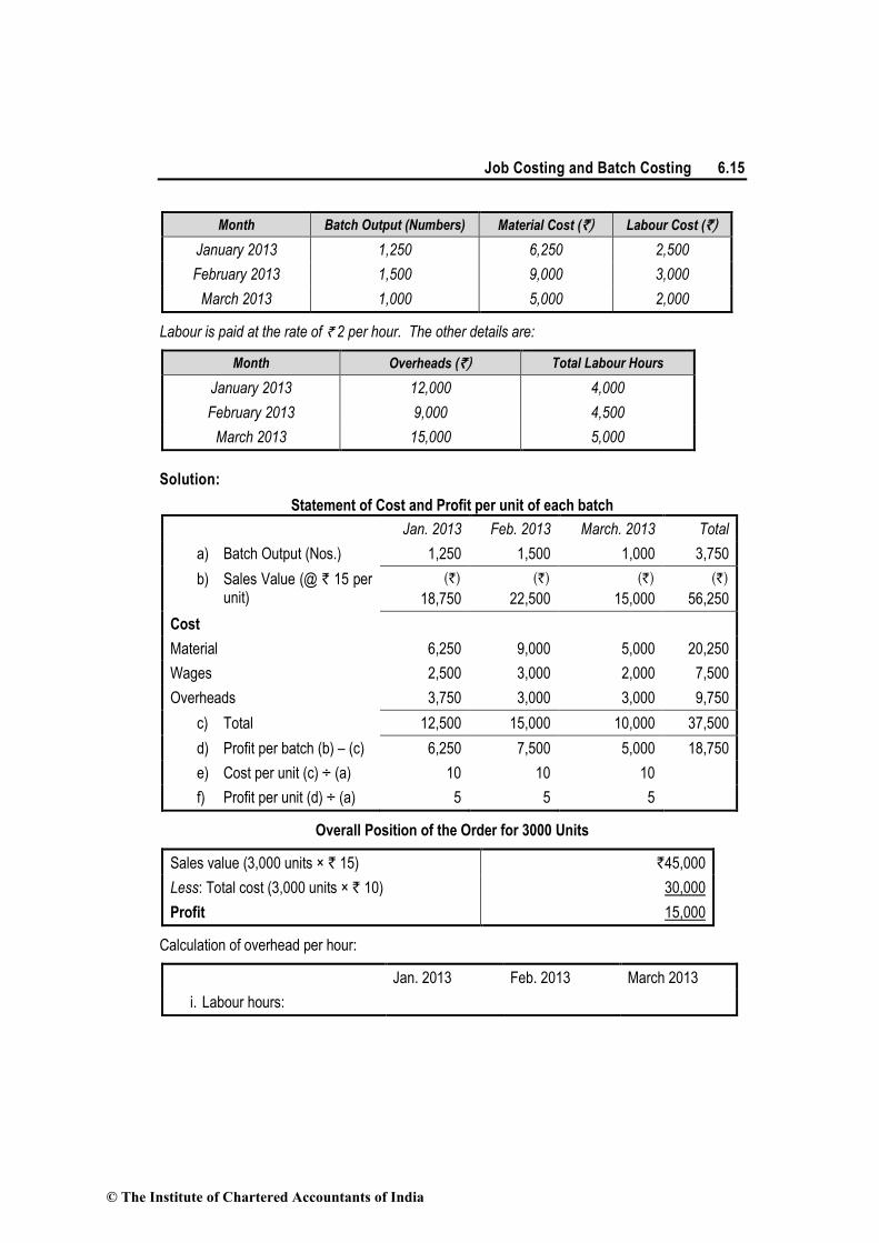
Job Costing and Batch Costing 6.15
Month Batch Output (Numbers) Material Cost (`) Labour Cost (`)
January 2013 1,250 6,250 2,500
February 2013 1,500 9,000 3,000
March 2013 1,000 5,000 2,000
Labour is paid at the rate of ` 2 per hour. The other details are:
Month Overheads (`) Total Labour Hours
January 2013 12,000 4,000
February 2013 9,000 4,500
March 2013 15,000 5,000
Solution:
Statement of Cost and Profit per unit of each batch
Jan. 2013 Feb. 2013 March. 2013 Total
a) Batch Output (Nos.) 1,250 1,500 1,000 3,750
b) Sales Value (@ ` 15 per unit)
(`)
18,750
(`)
22,500
(`)
15,000
(`)
56,250
Cost
Material 6,250 9,000 5,000 20,250
Wages 2,500 3,000 2,000 7,500
Overheads 3,750 3,000 3,000 9,750
c) Total 12,500 15,000 10,000 37,500
d) Profit per batch (b) – (c) 6,250 7,500 5,000 18,750
e) Cost per unit (c) ÷ (a) 10 10 10
f) Profit per unit (d) ÷ (a) 5 5 5
Overall Position of the Order for 3000 Units
Sales value (3,000 units × ` 15) `45,000
Less: Total cost (3,000 units × ` 10) 30,000
Profit 15,000
Calculation of overhead per hour:
Jan. 2013 Feb. 2013 March 2013
i. Labour hours:
© The Institute of Chartered Accountants of India

6.16 Cost Accounting
=Labour cost
Labour rates per hour
2,500
2
` = 1,250
3,000
2
`= 1,500
2,000
2
` = 1,000
ii. Overhead per hour :
=Total Overheads
Total labour hour
12,000
4,000
` = ` 3
9,000
4,500
` = ` 2
15,000
5,000
` = ` 3
iii. Overhead for batch (i) × (ii) ` 3,750 ` 3,000 ` 3,000
6.4.2 Economic Batch Quantity: In batch costing the most important problem is the
determination of optimum size of the batch (how much to produce) or Economic Batch
Quantity.
The determination of economic batch quantity involve two types of costs viz.,
(i) Set up cost (or preparation cost) and
(ii) Carrying cost.
With the increase in the batch size, there is an increase in the carrying cost but the set up cost
per unit of product is reduced; this situation is reversed when the batch size is reduced. Thus
there is one particular batch size for which both set up and carrying costs are minimum. This
size is known as economic or optimum batch quantity.
Economic batch quantity can be determined with the help of a table, graph or mathematical
formula. The mathematical formula usually used for its determination is as follows :
EBQ = 2 DS
C
Where, D = Annual demand for the product
S = Setting up cost per batch
C = Carrying cost per unit of production
Note : If the rate of interest (I) and unit cost of production (C) are given, the following formula
should be used for determining EBQ.
EBQ = 2 DS
C
Illustration 6 (Determination of economic batch quantity)
Monthly demand for a product 500 units
Setting-up cost per batch ` 60
Cost of manufacturing per unit ` 20
Rate of interest 10% p.a.
Determine economic batch quantity.
© The Institute of Chartered Accountants of India

Job Costing and Batch Costing 6.17
Solution:
EBQ = 2DS
C=
201.0
60125002
××××
= 600 units.
Illustration 7 (Calculation of EBQ and minimum inventory holding cost)
X Ltd. is committed to supply 24,000 bearings per annum to Y Ltd. on steady basis. It is
estimated that it costs 10 paise as inventory holding cost per bearing per month and that the
set-up cost per run of bearing manufacture is ` 324.
(a) What would be the optimum run size for bearing manufacture?
(b) Assuming that the company has a policy of manufacturing 6,000 bearings per run, how
much extra costs the company would be incurring as compared to the optimum run
suggested in (a) above?
(c) What is the minimum inventory holding cost?
Solution:
(a) Optimum production run size (Q) = 2DS
C
where,
D = No. of units to be produced within one year.
S = Set-up cost per production run
C = Carrying cost per unit per annum.
= 2DS
C=
2 ×24,000 × 324
0.10 ×12
` = 3,600 bearings.
(b) Total Cost (of maintaining the inventories) when production run size (Q) are 3,600 and
6,000 bearings respectively
Total cost = Total set-up cost + Total carrying cost.
When run size is 3,600 bearings
When run size is 6,000 bearings
Total set up cost =
600,3
000,24 × ` 324 = ` 2,160 = ×
000,6
000,24` 324 = ` 1,29
Total Carrying cost 1/2×3,600 × 0.10P × `12
= ` 2,160
1/2 × 6,000 × 0.10P × `12
= ` 3,600
Total Cost ` 4,320 ` 4,896
© The Institute of Chartered Accountants of India

6.18 Cost Accounting
(c) Minimum inventory holding cost = 1/2 Q × C
(when Q = 3,600 bearings) = 1/2 × 3,600 bearings × 0.10P × ` 12 = ` 2,160
6.5 Summary
Job Costing : Production/work done as per customer specification
Meaning of spoiled and defective work under job costing:-
♦ Spoiled :- Produced units cannot be rectified.
♦ Defective :- Units can be rectified with some additional cost.
Batch Costing :- Articles are produced in a lot and cost are computed per unit in a batch.
Cost per unit in a batch = Total cost of a batch/Number of item produced.
EBQ = Points where Set up and carrying cost are minimum.
EBQ = 2DS
C
© The Institute of Chartered Accountants of India

7 Contract Costing
Learning Objectives
When you have finished studying this chapter, you should be able to
• Understand the meaning of a contract and other terms used in contract costing.
• Compute profit of an incomplete contract, cost of contract and cost of work certified.
• Understand the meaning of escalation clause in contract and its impact on contract
price.
7.1 Introduction
A contract takes longer period to complete and the result of the contract can be known only
after the completion of the contract. If the profit on such contracts is calculated only after their
completion, then wide fluctuations may be noted in the profit figures of contractors from year
to year. The profit in respect of each contract in progress is transferred to the costing profit
and loss account of the year by calculating the notional profit. The portion of notional profit to
be transferred to the costing profit and loss account depends on the stage of completion of a
contract. To determine such a profit figure the knowledge of various concepts as discussed
below is essential in contract costing.
7.2 Meaning of Contract Costing
Contract costing is a form of specific order costing where job undertaken is relatively large and
normally takes period longer than a year to be getting completed. Contract costing is usually
adopted by the contractors engaged in the task of executing Civil Contracts. Contract costing
have the following distinct features:
1. The major part of the work in connection with each contract is ordinarily carried out at the
site of the contract.
2. The bulk of the expenses incurred by the contractor are considered as direct.
3. The indirect expenses mostly consist of office expenses of the yards, stores and works.
4. A separate account is usually maintained for each contract.
© The Institute of Chartered Accountants of India

7.2 Cost Accounting
5. The number of contracts undertaken by a contractor at a time is usually few.
6. The cost unit in contract costing is the contract itself.
7.3 Recording of contract costs
Material Cost: All materials supplied from the stores or purchased directly for the contract are
debited to the concerned contract account. In the case of transfer of excess material from one
contract to other contract, their costs would be adjusted on the basis of material transfer note,
signed both by the transferee and the transferor foreman. In case the return of surplus
material appears uneconomical on account of high cost of transportation, the same is sold and
the concerned contract account is credited with the sale price. Any loss or profit arising there-
from is transferred to the Costing Profit and Loss Account. Any theft or destruction of material
by fire represents a loss and as such, the same is transferred to the Costing Profit and Loss
Account. If any stores items are used for manufacturing tools, the cost of such stores items
are charged to the work expenses account. If the contractee has supplied some materials
without affecting the contract price, no accounting entries will be made in the contract account,
only a note may be given about it.
Labour Cost: Labour actually employed on the site of the contract is regarded as direct
(irrespective of the nature of the task performed) and the wages paid to them are charged to
the concerned contract directly or on the basis of a wage analysis sheet (if concurrently a
number of contracts are carried on and labourers are required to devote their time on two or
more contracts).
Direct Expenses: Direct expenses (if any) are directly charged to the concerned contract
account.
Indirect Expenses: Indirect expenses (such as expenses of engineers, surveyors,
supervisors etc.) may be distributed over several contracts as a percentage of cost of
materials, or wages paid or of the prime cost. If however, the contracts are big, the labour hour
method may be used for the distribution of expenses.
Plant and Machinery: The value of the plant in a contract may be either debited to contract
account and the written down value thereof at the end of the year entered on the credit side
for closing the contract account, or only a charge (depreciation) for use of the plant may be
debited to the contract account.
Sub-Contract: Sub-contract costs are also debited to the Contract Account.
Extra work: The extra work amount payable by the contractee should be added to the
contract price. If extra work is substantial, it is better to treat it as a separate contract. If it is
not substantial, expenses incurred should be debited to the contract account as “Cost of Extra
work”.
© The Institute of Chartered Accountants of India

Contract Costing 7.3
7.4 Meaning of the terms used in contract costing
(i) Cost of Work Certified or Value of Work Certified: A contract is a continuous process
and to know the cost or value of the work completed as on a particular date; assessment of
the work is carried out by the surveyor or architect. Surveyor or architect based on his
assessment certifies the percentage of work completion. This portion of called value or cost of
work certified.
Mathematically:
(a) Value of Work Certified = Value of Contract x Work certified (%)
(b) Cost of Work Certified = Cost of work to date – (Cost of work uncertified + Material in hand
+ Plant at site)
(ii) Progress Payment: Contractors receive payments from the contractee periodically for
the work done on the contract. This is known as progress payment or running payment. This is
paid based on the certificate issued by the surveyor or architect.
Mathematically:
Progress payment = Value of work certified – Retention money – Payment to date
(iii) Retention Money: A contractor does not receive full payment of the work certified by the
surveyor. Contractee retains some amount (say 10% to 20%) to be paid, after sometime, when it is
ensured that there is no fault in the work carried out by contractor. If any deficiency or defect is
noticed in the work, it is to be rectified by the contractor before the release of the retention money.
Retention money provides a safeguard against the risk of loss due to faulty workmanship.
Mathematically:
Retention Money = Value of work certified – Payment actually made/ cash paid
(iv) Cost of Work Uncertified: It represents the cost of the work which has been carried out
by the contractor but has not been certified by the architect. It is always shown at cost price.
The cost of uncertified work may be ascertained as follows:
(`) (`)
Total cost to date —
Less: Cost of work certified —
Material in hand —
Plant at site — —
Cost of work uncertified —
(v) Cash Received: It is ascertained by deducting the retention money from the value of
work certified i.e.
© The Institute of Chartered Accountants of India

7.4 Cost Accounting
Cash received = Value of work certified – Retention money.
(vi) Work-in-Progress: In Contract Accounts, the value of the work-in-progress consists of
(i) the cost of work completed, both certified and uncertified;
(ii) the cost of work not yet completed; and
(iii) the amount of profit taken as credit.
In the Balance Sheet (prepared for management), the work-in-progress is usually shown under
two heads, viz., certified and uncertified. The cost of work completed and certified and the
profit credited will appear under the head ‘certified’ work-in-progress, while the completed
work not yet certified and the cost of labour, material and expenses of work which has not yet
reached the stage of completion are shown under the head “uncertified” work-in-progress.
(vii) Notional Profit: It represents the difference between the value of work certified and cost
of work certified. It is determined:
Notional profit = Value of work certified – (Cost of work to date – Cost of work not yet certified)
(viii) Estimated Profit: It is the excess of the contract price over the estimated total cost of
the contract.
Illustration 1 (Computation of estimated profit)
Compute a conservative estimate of profit on a contract (which has been 90% complete) from
the following particulars: (`)
Total expenditure to date 22,50,000
Estimated further expenditure to complete the contract (including contingencies) 2,50,000
Contract price 32,50,000
Work certified 27,50,000
Work uncertified 1,75,000
Cash received 21,25,000
Solution:
Calculation of conservative Estimate of Profit (`)
Total expenditure to date 22,50,000
Estimated further expenditure to complete the contract
(including contingencies)
2,50,000
25,00,000
Estimated profit on contract 7,50,000
Contract price 32,50,000
Profit to be transferred to Contract Profit and Loss A/c
© The Institute of Chartered Accountants of India

Contract Costing 7.5
Estimated Profit × Cash Received
Contract Price
= ` 7,50,000 × `
`
21,25,000
32,50,000 = ` 4,90,385
7.5 Profit/loss on incomplete contracts
To determine the profit to be taken to Costing Profit and Loss Account, in the case of
incomplete contracts, the following four situations may arise:
Students may note that profit/ loss determined here is on the basis of prudence and for the internal
managerial decision making purpose only. For financial reporting purpose, profit/ loss from a contract is
to be determined in accordance with relevant Accounting Standards in force.
Note: “Students are requested to refer the Study Material and Practice Manual of ‘Accounting’ (Paper-1
CA-Intermediate) to see and learn financial accounting perspective of contract accounting and
applicability of Accounting Standard- 7. Here only specific aspect of Contract Costing is discussed.”
(i) Completion of contract is less than 25 per cent: In this case no profit should be taken
to Costing Profit and Loss Account.
(ii) Completion of contract is 25 per cent or more but less than 50 per cent: In this case
one-third of the notional profit, reduced in the ratio of cash received to work certified,
should be transferred to the Costing Profit and Loss Account. Mathematically:
1 Cash receivedNotional Pr ofit
3 Work certified× ×
(iii) Completion of contract is 50 per cent or more but less than 90 per cent: In this case,
two-third of the notional profit, reduced by proportion of cash received to work certified, is
transferred to the Costing Profit and Loss Account. Mathematically:
2 Cash receivedNotional Pr ofit
3 Work certified× ×
(iv) Completion of contract is 90 per cent or more i.e. it is nearing completion: In this case
the profit to be taken to Costing Profit and Loss Account is computed by determining the
estimated profit and using any one of the following formulas:
(a) Estimated Profit × Work certified
Contract price
(b) Estimated Profit × Work certified
Contract price ×
certified Work
received Cash
© The Institute of Chartered Accountants of India

7.6 Cost Accounting
OR
Estimated Profit × Cash received
Contract price
(c) Estimated Profit × cost total Estimated
date to workofCost
(d) Estimated Profit × Cost of work to date
Estimated total cost ×
Cash received
Work certified
(e) Notional Profit × Work certified
Contract price
(This formula may be preferably used in the absence of estimated profit figure).
[It is preferable to use formula (b) in the absence of specific instructions.]
7.6 Cost plus contract
Under Cost plus Contract, the contract price is ascertained by adding a percentage of profit to
the total cost of the work. Such types of contracts are entered into when it is not possible to
estimate the contract cost with reasonable accuracy due to unstable condition of factors that
affect the cost of material, labour services, etc.
Cost plus contracts have the following advantages and disadvantages:
Advantages:
(i) The Contractor is assured of a fixed percentage of profit. There is no risk of incurring any
loss on the contract.
(ii) It is useful specially when the work to be done is not definitely fixed at the time of making
the estimate.
(iii) Contractee can ensure himself about ‘the cost of the contract’, as he is empowered to
examine the books and documents of the contractor to ascertain the veracity of the cost
of the contract.
Disadvantages - The contractor may not have any inducement to avoid wastages and effect
economy in production to reduce cost.
Escalation Clause - If during the period of execution of a contract, the prices of materials, or
labour etc., rise beyond a certain limit, the contract price will be increased by an agreed
amount. Inclusion of such a clause in a contract deed is called an “Escalation Clause”.
Illustration 2 (Preparation of contract account)
The following expenses were incurred on a contract : (`)
Material purchased 6,00,000
Material drawn from stores 1,00,000
© The Institute of Chartered Accountants of India

Contract Costing 7.7
Wages 2,25,000
Plant issued 75,000
Chargeable expenses 75,000
Apportioned indirect expenses 25,000
The contract was for ` 20,00,000 and it commenced on January 1, 2011. The value of the work
completed and certified upto 30th November, 2011 was ` 13,00,000 of which ` 10,40,000 was
received in cash, the balance being held back as retention money by the contractee. The value of
work completed subsequent to the architect’s certificate but before 31st December, 2011 was
` 60,000. There were also lying on the site materials of the value of ` 40,000. It was estimated that
the value of plant as at 31st December, 2011 was ` 30,000.
Solution
Dr. Contract Account Cr.
(`) (`)
To Material purchased 6,00,000 By Work-in-progress :
” Stores issued 1,00,000 Work certified 13,00,000
” Wages 2,25,000 Work uncertified 60,000
” Plant 75,000 Material unused 40,000
” Chargeable expenses 75,000 Plant less depreciation 30,000
” Indirect expenses 25,000
” Profit and Loss Account,
2/3rds of profit on cash basis 1,76,000*
” Work-in-progress balance of profit c/d 1,54,000 ________
14,30,000 14,30,000
” Balance b/d: Work certified 13,00,000
Uncertified 60,000
Material at site 40,000
Plant at site 30,000
14,30,000
Less: Reserve 1,54,000
12,76,000
* Computation of Profit : (`)
Apparent profit 3,30,000
2/3rd of that since 65% of the work is complete 2,20,000 80% of that on cash basis 1,76,000
An alternative method of presentation can be to deduct the balance of profit to be carried down (` 1,54,000 in the above case) from the work certified before it is entered in the contract account. It will be ` 11,46,000 in the illustration given above. Of course, the reserve to be so deducted from the work certified will have to be first ascertained by considering the value of the work certified.
© The Institute of Chartered Accountants of India
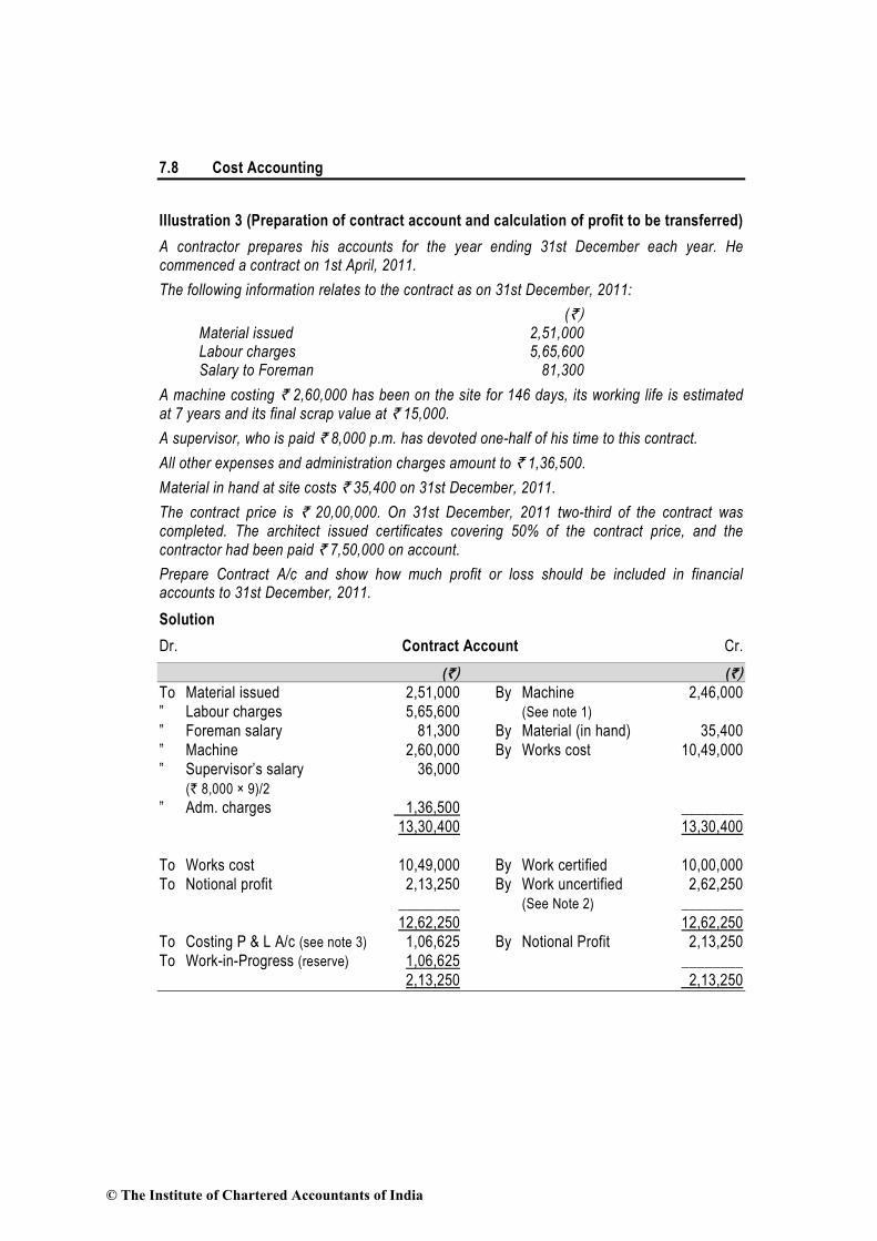
7.8 Cost Accounting
Illustration 3 (Preparation of contract account and calculation of profit to be transferred)
A contractor prepares his accounts for the year ending 31st December each year. He commenced a contract on 1st April, 2011.
The following information relates to the contract as on 31st December, 2011:
(`) Material issued 2,51,000 Labour charges 5,65,600 Salary to Foreman 81,300
A machine costing ` 2,60,000 has been on the site for 146 days, its working life is estimated at 7 years and its final scrap value at ` 15,000.
A supervisor, who is paid ` 8,000 p.m. has devoted one-half of his time to this contract.
All other expenses and administration charges amount to ` 1,36,500.
Material in hand at site costs ` 35,400 on 31st December, 2011.
The contract price is ` 20,00,000. On 31st December, 2011 two-third of the contract was completed. The architect issued certificates covering 50% of the contract price, and the contractor had been paid ` 7,50,000 on account.
Prepare Contract A/c and show how much profit or loss should be included in financial accounts to 31st December, 2011.
Solution
Dr. Contract Account Cr.
(`) (`)
To Material issued 2,51,000 By Machine 2,46,000
” Labour charges 5,65,600 (See note 1)
” Foreman salary 81,300 By Material (in hand) 35,400
” Machine 2,60,000 By Works cost 10,49,000
” Supervisor’s salary 36,000
(` 8,000 × 9)/2
” Adm. charges 1,36,500 ________
13,30,400 13,30,400
To Works cost 10,49,000 By Work certified 10,00,000
To Notional profit 2,13,250 By Work uncertified 2,62,250
________ (See Note 2) ________
12,62,250 12,62,250
To Costing P & L A/c (see note 3) 1,06,625 By Notional Profit 2,13,250
To Work-in-Progress (reserve) 1,06,625 ________
2,13,250 2,13,250
© The Institute of Chartered Accountants of India

Contract Costing 7.9
Notes :
1. Machine :
[(` 2,60,000 – ` 15,000) ÷ 7] × 365
146 = ` 14,000
Hence the value of machine after the period of 146 days is
` 2,60,000 – ` 14,000 = ` 2,46,000
2. The cost of 66.67% of the contract is ` 10,49,000
∴Cost of 100% " " " " ` 10,49,000
66.67 × 100 = ` 15,73,500
∴Cost of 50% of the contract which has been certified by the architect is `7,86,750. Also
the cost of 16.67% of the contract, which has been completed but not certified by the
architect is ` 2,62,250.
3. 2 Cash received
×Notional Profit ×3 Work certified
or, 2 7,50,000
× 2,13,250 ×3 10,00,000
= ` 1,06,625
Illustration 4 (Preparation of contract account, contractee account extracts of B/S)
M/s. Bansals Construction Company Ltd. took a contract for ` 60,00,000 expected to be
completed in three years. The following particulars relating to the contract are available:
2011 2012 2013
(`) (`) (`)
Materials 6,75,000 10,50,000 9,00,000
Wages 6,20,000 9,00,000 7,50,000
Cartage 30,000 90,000 75,000
Other expenses 30,000 75,000 24,000
Cumulative work certified 13,50,000 45,00,000 60,00,000 Cumulative work uncertified 15,000 75,000 —
Plant costing ` 3,00,000 was bought at the commencement of the contract. Depreciation was
to be charged at 25% per annum, on the written down value method. The contractee pays
75% of the value of work certified as and when certified, and makes the final payment on
completion of the contract.
You are required to make a contract account and contractee account as they would appear in
each of the three years. Also show how the work-in-progress and other items should appear in
the balance sheet.
© The Institute of Chartered Accountants of India

7.10 Cost Accounting
Solution
Dr. Contract Account Cr.
2011 (`) 2011 (`)
To Materials 6,75,000 By Plant at site c/d 2,25,000
To Wages 6,20,000 By Work-in-progress c/d : (`)
To Cartage 30,000 Work certified 13,50,000
To Other expenses 30,000 Work uncertified 15,000 13,65,000
To Plant 3,00,000 By Costing P & L A/c 65,000
________ (Loss transferred) ________
16,55,000 16,55,000
2012 (`) 2012 (`)
To Work-in-progress b/d : By Work-in-progress c/d :
Work certified 13,50,000 Work certified 45,00,000
Work uncertified 15,000 13,65,000 Work uncertified 75,000 45,75,000
To Plant b/d 2,25,000 By Plant at site c/d 1,68,750
To Materials 10,50,000
To Wages 9,00,000
To Cartage 90,000
To Other expenses 75,000
To Notional profit c/d 10,38,750
47,43,750 47,43,750
To Costing P & L A/c 5,19,375 By Notional profit b/d 10,38,750
To Work-in-progress c/d 5,19,375
(profit in reserve)
(Refer to working note 2) ________ ________
10,38,750 10,38,750
2013 (`) 2013 (`)
To Work-in-progress b/d: By Work-in-progress b/d 5,19,375
Work certified 45,00,000 (profit in reserve)
Work uncertified 75,000 45,75,000 By Plant at site 1,26,562
By Contractee’s A/c 60,00,000
© The Institute of Chartered Accountants of India
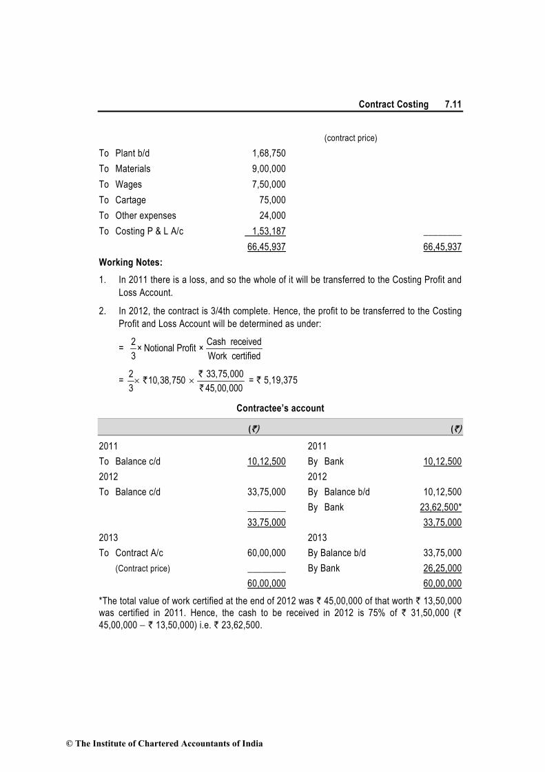
Contract Costing 7.11
(contract price)
To Plant b/d 1,68,750
To Materials 9,00,000
To Wages 7,50,000
To Cartage 75,000
To Other expenses 24,000
To Costing P & L A/c 1,53,187 ________
66,45,937 66,45,937
Working Notes:
1. In 2011 there is a loss, and so the whole of it will be transferred to the Costing Profit and
Loss Account.
2. In 2012, the contract is 3/4th complete. Hence, the profit to be transferred to the Costing
Profit and Loss Account will be determined as under:
= 2 Cash received
× Notional Profit ×3 Work certified
= 2 33,75,000
10,38,7503 45,00,000× ×
` `
` = ` 5,19,375
Contractee’s account
(`) (`)
2011 2011
To Balance c/d 10,12,500 By Bank 10,12,500
2012 2012
To Balance c/d 33,75,000 By Balance b/d 10,12,500
________ By Bank 23,62,500*
33,75,000 33,75,000
2013 2013
To Contract A/c 60,00,000 By Balance b/d 33,75,000
(Contract price) ________ By Bank 26,25,000
60,00,000 60,00,000
*The total value of work certified at the end of 2012 was ` 45,00,000 of that worth ` 13,50,000
was certified in 2011. Hence, the cash to be received in 2012 is 75% of ` 31,50,000 (`
45,00,000 − ` 13,50,000) i.e. ` 23,62,500.
© The Institute of Chartered Accountants of India

7.12 Cost Accounting
Balance Sheet (Extract) 2011
Liabilities (`) Assets (`)
Capital − Plant at site 2,25,000
Less : Loss during the year 65,000
Work-in-progress : (`)
Work certified 13,50,000
Work uncertified 15,000
13,65,000
Less: Cash received 10,12,500 3,52,500
Balance sheet (Extract) 2012
Liabilities (`) Assets (`)
Capital − Plant at site 1,68,750
Add: Profit during the year 5,19,375 Work-in-progress : (`)
Work certified 45,00,000
Work uncertified 75,000
45,75,000
Less: Profit in reserve 5,19,375
40,55,625
Less: Cash received 33,75,000 6,80,625
Balance sheet (Extract) 2013
Liabilities (`) Assets (`)
Capital − Plant at site 1,26,562
Add: Profit during the year 1,53,187
Illustration 5 (Computation of conservative estimate of profit)
Compute a conservative estimate of profit on a contract (which has been 90% complete) from
the following particulars. Calculate the proportion of profit to be taken to Costing Profit & Loss
Account under various methods and give your recommendation.
(`) Total expenditure to date 4,50,000
Estimated further expenditure to complete the contract (including contingencies) 25,000
Contract price 6,12,000
© The Institute of Chartered Accountants of India
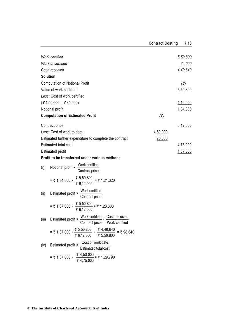
Contract Costing 7.13
Work certified 5,50,800
Work uncertified 34,000
Cash received 4,40,640
Solution
Computation of Notional Profit (`)
Value of work certified 5,50,800
Less: Cost of work certified
(` 4,50,000 – ` 34,000) 4,16,000
Notional profit 1,34,800
Computation of Estimated Profit (`)
Contract price 6,12,000
Less: Cost of work to date 4,50,000
Estimated further expenditure to complete the contract 25,000
Estimated total cost 4,75,000
Estimated profit 1,37,000
Profit to be transferred under various methods
(i) Notional profit × priceContract
certified Work
= ` 1,34,800 × `
`
5,50,800
6,12,000 = ` 1,21,320
(ii) Estimated profit × priceContract
certified Work
= ` 1,37,000 × `
`
5,50,800
6,12,000= ` 1,23,300
(iii) Estimated profit × Work certified
Contract price×
Cash received
Work certified
= ` 1,37,000 ×`
`
5,50,800
6,12,000 ×
`
`
4,40,640
5,50,800 = ` 98,640
(iv) Estimated profit × Cost of work date
Estimated total cost
= ` 1,37,000 × `
`
4,50,000
4,75,000= ` 1,29,790
© The Institute of Chartered Accountants of India

7.14 Cost Accounting
(v) Estimated profit × Cost of work date
Estimated total cost ×
Cash received
Work certified
= ` 1,37,000 × `
`
4,50,000
4,75,000 ×
`
`
4,40,640
5,50,800 = ` 1,03,832
Recommendation: It is recommended that a sum of ` 98,640 may be transferred to the
Costing Profit and Loss Account. This amount is the least and has been arrived by using the
formula (iii) above. According to this formula, profit transferred to the Costing Profit and Loss
Account is generally kept the minimum and allows withholding in reserve a larger portion of
notional profit to meet future unforeseen expenses and contingencies.
Illustration 6 (Calculation of admissible escalation claim)
A contractor has entered into a long term contract at an agreed price of ` 1,75,000 subject to
an escalation clause for materials and wages as spelt out in the contract and corresponding
actual are as follows :
Standard Actual
Materials Qty (tonnes) Rate (`) Qty (tonnes) Rate (`)
A 5,000 5 5,050 4.80
B 3,500 8 3,450 7.90
C 2,500 6 2,600 6.60
Labour Hours Hourly Hours Hourly
Rate (`) Rate (`)
X 2,000 7.00 2,100 7.20
Y 2,500 7.50 2,450 7.50 Z 3,000 6.50 3,100 6.60
Reckoning the full actual consumption of material and wages the company has claimed a final
price of ` 1,77,360. Give your analysis of admissible escalation claim and indicate the final
price payable.
Solution
Statement showing final claim
Standard Standard Actual Rate Variation in Escalation
Qty/Hrs. Rate (`) (`) Rate (`) Claim (`)
Materials (a) (b) (c) (d) = (c)–(b) (e) =(a) × (d)
A 5,000 5.00 4.80 (–) 0.20 (–) 1,000
B 3,500 8.00 7.90 (–) 0.10 (–) 350
C 2,500 6.00 6.60 (+) 0.60 1,500
Materials escalation claim : (P) 150
Labour
X 2,000 7.00 7.20 (+) 0.20 400
© The Institute of Chartered Accountants of India

Contract Costing 7.15
Y 2,500 7.50 7.50 − −
Z 3,000 6.50 6.60 (+) 0.10 300
Wages escalation claim : (Q) 700
Final claim: (P) + (Q) 850
Statement showing final price payable
Agreed price ` 1,75,000
Agreed escalation :
Material cost ` 150
Labour cost ` 700 ` 850
Final price payable ` 1,75,850
The claim of ` 1,77,360 is based on the total increase in cost. This can be verified as shown
below:
Statement showing total increase in cost
Standard Cost Actual Cost Increase/
Qty/hrs Rate Amount Qty/hrs Rate Amount (Decrease)
(`) (`) (`) (`)
(a) (b) (c) = (a) × (b) (d) (e) (f) =(d) × (e) (g) =(f) – (c)
I. Materials
A 5,000 5.00 25,000 5,050 4.80 24,240 (760)
B 3,500 8.00 28,000 3,450 7.90 27,255 (745)
C 2,500 6.00 15,000 2,600 6.60 17,160 2,160
68,000 68,655 655
II. Labour
X 2,000 7.00 14,000 2,100 7.20 15,120 1,120
Y 2,500 7.50 18,750 2,450 7.50 18,375 (375)
Z 3,000 6.50 19,500 3,100 6.60 20,460 960
52,250 53,955 1,705
Total (I + II) 2,360
The final price claimed by the company is contract price ` 1,75,000
Add : Increase in cost ` 2,360
` 1,77,360
This claim is not admissible because escalation clause covers only that part of increase in
cost, which has been caused by inflation.
Note : It is fundamental principle that the contractee would compensate the contractor for the
increase in costs which are caused by factors beyond the control of contractor and not for
increase in costs which are caused due to inefficiency or wrong estimation.
© The Institute of Chartered Accountants of India

7.16 Cost Accounting
Illustration 7 (Preparation of contract account and calculation of estimated profit)
AKP Builders Ltd. commenced a contract on April 1, 2012. The total contract was for
` 5,00,000. Actual expenditure for the period April 1, 2012 to March 31, 2013 and estimated
expenditure for April 1, 2013 to December 31, 2013 are given below :
Particulars 2012-13
(actual)
2013-14
(9 months)
(estimated)
Materials issued 90,000 85,750
Labour : Paid 75,000 87,325
Outstanding at the end 6,250 8,300
Plant 25,000 -
Sundry expenses : Paid 7,250 6,875
Prepaid at the end 625 -
Establishment charges 14,625 -
A part of the material was unsuitable and was sold for `18,125 (cost being `15,000) and a
part of plant was scrapped and disposed of for `2,875. The value of plant at site on 31 March,
2013 was ` 7,750 and the value of material at site was ` 4,250. Cash received on account to
date was ` 1,75,000, representing 80% of the work certified. The cost of work uncertified was
valued at ` 27,375.
The contractor estimated further expenditure that would be incurred in completion of the contract :
The contract would be completed by 31st December, 2013.
A further sum of `31,250 would have to be spent on the plant and the residual value of
the plant on the completion of the contract would be `3,750.
Establishment charges would cost the same amount per month as in the previous year.
` 10,800 would be sufficient to provide for contingencies.
Required: Prepare Contract Account and calculate estimated total profit on this contract. Profit
transferrable to Costing Profit and Loss Account is to be calculated by reducing estimated
profit in proportion of work certified and contract price.
Solution AKP Builders Ltd.
Contract Account (2012-13)
Particulars (`) Particulars (`)
To Materials issued 90,000 By Material sold 18,125
To Labour 75,000 By Plant sold 2,875
Add: Outstanding 6,250 81,250 By Plant at site 7,750
To Plant 25,000 By Material at site 4,250
© The Institute of Chartered Accountants of India

Contract Costing 7.17
To Sundry Expenses 7,250 By Work-in-progress
Less : Prepaid 625 6,625 Work certified 2,18,750
To Establishment charges 14,625 Work uncertified 27,375 2,46,125
To Costing P & L A/c 3,125
(profit on sale of
material)
To Notional profit c/d 58,500
2,79,125 2,79,125
To Costing P & L A/c
(transfer)
29,960 By Notional profit b/d 58,500
To Work-in-progress (reserve) 28,540
58,500 58,500
Profit to be transferred to Costing Profit and Loss Account
= Estimated profit ×priceContract
CertifiedWork
= ` 68,481 × 2,18,750
5,00,000 = ` 29,960
Calculation of Estimated Profit (`)
(1) Material consumed (90,000 + 3,125 – 18,125) 75,000
Add : Further consumption 85,750 1,60,750
(2) Plant used (25,000 – 2,875) 22,125
Add: Further plant introduced 31,250
Less: Closing balance of plant 3,750 49,625
(3) Establishment charges 14,625
Add: Further charges for nine month (14,625 × 9/12) 10,969 25,594
(4) Sundry expenses 6,625
Add: Further expenses 6,875
Add: Prepaid expenses 625 14125
(5) Labour cost 81,250
Add: Further cost (87,325 – 6,250) 81,075
Add: Outstanding 8,300 1,70,625
(6) Reserve for contingencies 10,800
Estimated profit (balancing figure) 68,481
Contract price 5,00,000
© The Institute of Chartered Accountants of India

7.18 Cost Accounting
Illustration 8 (Preparation of contract account and determination of profit)
RST Construction Ltd. commenced a contract on April 1, 2011. The total contract was for
` 49,21,875. It was decided to estimate the total profit on the contract and to take to the credit
of Costing Profit and Loss A/c that proportion of estimated profit on cash basis, which work
completed bore to total contract. Actual expenditure for the period April 1, 2011 to March 31,
2012 and estimated expenditure for April 1, 2012 to September 30, 2012 are given below:
April 1, 2011 to
March 31, 2012
(Actual) (`)
April 1, 2012 to
Sept. 30, 2012
(Estimated) (`)
Materials issued 7,76,250 12,99,375
Labour : Paid 5,17,500 6,18,750
Prepaid 37,500 -
Outstanding 12,500 5,750
Plant purchased 4,00,000 -
Expenses: Paid 2,25,000 3,75,000
Outstanding 25,000 10,000
Prepaid 15,000 -
Plant returns to store (historical cost) 1,00,000 3,00,000
(on September 30, 2011) (on September 30, 2012)
Work certified 22,50,000 Full
Work uncertified 25,000 -
Cash received 18,75,000 -
Materials at site 82,500 42,500
The plant is subject to annual depreciation @ 25% on written down value method. The
contract is likely to be completed on September 30, 2012.
Required : Prepare the Contract A/c. Determine the profit on the contract for the year 2011-12
on prudent basis, which has to be credited to Costing Profit and Loss A/c.
Solution
Calculation of written down value of plant as on 30-9-2012. (`)
Plant purchased on 1-4-2011 4,00,000
Less: Plant returned to store on 30-9-2011 1,00,000
(Depreciation on it `1,00,000 × 25/100 × 6/12 = `12,500)
3,00,000
Less: Depreciation on Balance plant (3,00,000 × 25/100) 75,000
WDV of Plant on 1-4-2012 2,25,000
Less : Depreciation (2,25,000 × 25/100 × 6/12) 28,125
WDV of plant returned to store on 30-9-2012 1,96,875
© The Institute of Chartered Accountants of India

Contract Costing 7.19
Contract A/c (1-4-2011 to 31-3-2012)
Particulars (`) Particulars (`)
To Materials issued 7,76,250 By Plant returned to
To Labour 5,17,500 Store on 30-9-2011 1,00,000
Less: Prepaid 37,500 Less: Depreciation(1/2)
12,500 87,500
4,80,000
Add : Outstanding 12,500 4,92,500 By Plant at site on 31.3.12
3,00,000
To Plant purchased 4,00,000 Less: Depreciation 75,000 2,25,000
To Expenses 2,25,000 By Materials at site 82,500
Less : Prepaid 15,000 By Work-in-progress
2,10,000 Work certified 22,50,000
Add : Outstanding 25,000 2,35,000 Work uncertified 25,000
To Notional profit c/d 7,66,250 -
26,70,000 26,70,000
To Costing P&L A/c (Transfer)
3,89,000 By Notional profit b/d 7,66,250
To Work-in-progress (Reserve)
3,77,250
-
7,66,250 7,66,250
Computation of Estimated Profit Contract A/c (1-4-2011 to 30-9-2012)
Particulars (`) Particulars (`)
To Materials issued (7,76,250+12,99,375)
20,75,625 By Materials at site 42,500
To Labour (5,17,500 - 37,500 + 12,500 + 6,18,750+37,500 -12,500 + 5,750)
11,42,000 By Plant returned to store on 30.9.2011 (1,00,000 – 12,500)
87,500
To Plant purchased 4,00,000 By Plant returned to store on 30.9.12 (4,00,000 – 1,00,000 – 1,03,125)
1,96,875
To Expenses (2,25,000+25,000 -15,000+ 3,75,000 - 25,000 + 15,000 + 10,000)
6,10,000 By Contractee A/c 49,21,875
To Estimated profit 10,21,125 ________ 52,48,750 52,48,750
© The Institute of Chartered Accountants of India
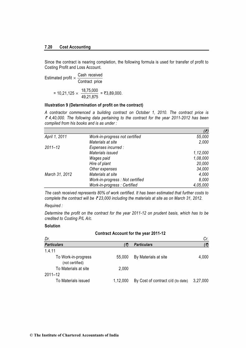
7.20 Cost Accounting
Since the contract is nearing completion, the following formula is used for transfer of profit to
Costing Profit and Loss Account.
Estimated profit ×price Contract
received Cash
= 10,21,125 × 49,21,875
18,75,000 = `3,89,000.
Illustration 9 (Determination of profit on the contract)
A contractor commenced a building contract on October 1, 2010. The contract price is
` 4,40,000. The following data pertaining to the contract for the year 2011-2012 has been
compiled from his books and is as under :
(`)
April 1, 2011 Work-in-progress not certified 55,000
Materials at site 2,000
2011–12 Expenses incurred :
Materials issued 1,12,000
Wages paid 1,08,000
Hire of plant 20,000
Other expenses 34,000
March 31, 2012 Materials at site 4,000
Work-in-progress : Not certified 8,000 Work-in-progress : Certified 4,05,000
The cash received represents 80% of work certified. It has been estimated that further costs to
complete the contract will be ` 23,000 including the materials at site as on March 31, 2012.
Required :
Determine the profit on the contract for the year 2011-12 on prudent basis, which has to be
credited to Costing P/L A/c.
Solution
Contract Account for the year 2011-12
Dr. Cr.
Particulars (`) Particulars (`)
1.4.11
To Work-in-progress 55,000 By Materials at site 4,000
(not certified)
To Materials at site 2,000
2011–12
To Materials issued 1,12,000 By Cost of contract c/d (to date) 3,27,000
© The Institute of Chartered Accountants of India

Contract Costing 7.21
To Wages paid 1,08,000
To Hire of plant 20,000
To Other expenses 34,000 _______
3,31,000 3,31,000
31.3.12
To Cost of contract b/d 3,27,000 By Work-certified 4,05,000
(to date) By Work-not certified 8,000
To Costing P& L A/c 66,273
To Profit in reserve 19,727 _______
4,13,000 4,13,000
Profit for the year 2011-12 = ` 4,13,000 – ` 3,27,000 = ` 86,000
Estimated profit (on the completion of the contract)
(`)
Cost of the contract (to date) 3,27,000
Further cost of completing the contract 23,000
Total cost: (A) 3,50,000
Contract price: (B) 4,40,000
Estimated profit on the completion of contract: {(A) – (B)} 90,000
Since,
priceContract
certified Work × 100 =
`
`
4,05,000
4,40,000 × 100 = 92.05%
Profit = Estimated profit ×price Contract
received Cash
= ` 90,000 × 3,24,000
4,40,000 = ` 66,273
Illustration 10 (Determination of profit for the contracts)
A construction company under-taking a number of contracts, furnished the following data
relating to its uncompleted contracts as on 31st March, 2012 :
(` in lacs)
Contract Numbers
723 726 729 731
Total Contract Price 23.20 14.40 10.08 28.80
Estimated Costs on completion of contract 20.50 11.52 12.60 21.60
Expenses for the year ended 31.3.12 :
Direct Materials 5.22 1.80 1.98 0.80
Direct Wages 2.32 4.32 3.90 2.16
© The Institute of Chartered Accountants of India

7.22 Cost Accounting
Overheads (Excluding Depreciation) 1.06 2.60 2.62 1.05
Profit Reserve as on 1.4.11 1.50 — — —
Plant issued at Cost 5.00 3.50 2.75 3.00
Materials at Site on 1.4.11 0.75 — — —
Materials at Site on 31.3.12 0.45 0.20 0.08 0.05
Work Certified till 31.3.11 4.65 — — —
Work Certified during the year 2011-12 12.76 13.26 7.56 4.32
Work Uncertified as on 31.3.12 0.84 0.24 0.14 0.18
Progress payments received during the year 9.57 9.0 5.75 3.60
Depreciation @ 20% per annum is to be charged on plant issued. While the Contract No. 723
was carried over from last year, the remaining contracts were started in the 1st week of April,
2011.
Required:
(i) Determine the profit/loss in respect of each contract for the year ended 31st March,
2012.
(ii) State the profit/loss to be carried to Profit & Loss A/c for the year ended 31st March,
2012.
Solution
(i) Statement of Profit/Loss for the year ended 31st March, 2012 (` in lacs)
Contract Numbers
723 726 729 731
A. Contract completion percentage :
Work certified : (a) 17.41 13.26 7.56 4.32
Contract price : (b) 23.20 14.40 10.08 28.80
Percentage of completion : [(a) – (b)] 75.04 92.08 75.00 15.00
B. Estimated profit on completion :
Contract price : (c) 23.20 14.40 10.08 28.80
Estimated costs on completion : (d) 20.50 11.52 12.60 21.60
Estimated profit (loss) on completion : [(c) – (d)] 2.70 2.88 (2.52) 7.20
C. Profit of the year :
Opening stock of materials 0.75 — — —
Materials issued 5.22 1.80 1.98 0.80
Direct wages 2.32 4.32 3.90 2.16
Overheads 1.06 2.60 2.62 1.05
Depreciation 1.00 0.70 0.55 0.60
Total : (P) 10.35 9.42 9.05 4.61
© The Institute of Chartered Accountants of India

Contract Costing 7.23
Profit in reserve 1.50 — — —
Material at site on 31/3/12 0.45 0.20 0.08 0.05
Total : (Q) 1.95 0.20 0.08 0.05
Cost of contract : (R) = [(P) – (Q)] 8.40 9.22 8.97 4.56
Work certified 12.76 13.26 7.56 4.32
Work not certified 0.84 0.24 0.14 0.18
Total : (S) 13.60 13.50 7.70 4.50
Profit (loss) for the year [(R) – (S)] 5.20 4.28 (1.27) (0.06)
(ii) Profit to be taken to Costing Profit & Loss Account of the year in respect of
respective contract
Contract 723 = 3
2× Notional profit ×
Cash received
Work certified
= 3
2 × 5.20 ×
9.57
17.41 = ` 1.9056 lacs
= Balance ` 3.2944 lacs to reserve.
Contract 726 = Estimated total profits on completion × Work certified
Contract price ×
Cash received
Work certified
= ` 2.88 × 13.26
14.40 ×
9.0
13.26 = ` 1.80
Illustration 11 (Preparation of contract account and determination of profit)
MNP Construction Ltd. commenced a contract on April 1, 2010. The total contract was for
` 17,50,000. It was decided to estimate the total profit and to take to the credit of Costing P/L
A/c the proportion of estimated profit on cash basis which work completed bore to the total
contract. Actual expenditure in 2010-11 and estimated expenditure in 2011-2012 are given
below:
2010-2011 2011-2012
(Actual) (Estimated)
(`) (`)
Materials issued 3,00,000 5,50,000
Labour : Paid 2,00,000 2,50,000
: Outstanding at end 20,000 30,000
Plant purchased 1,50,000 —
Expenses : Paid 75,000 1,50,000
: Prepaid at end 15,000 —
Plant returns to store (historical cost) 50,000 1,00,000
© The Institute of Chartered Accountants of India

7.24 Cost Accounting
(on Dec. 31, 2011)
Material at site 20,000 50,000
Work certified 8,00,000 Full
Work uncertified 25,000 —
Cash received 6,00,000 Full
The plant is subject to annual depreciation @ 25% of WDV Cost. The contract is likely to be
completed on Dec. 31, 2011. Prepare the Contract A/c. Determine the profit on the contract for
the year 2010-2011 on prudent basis, which has to be credited to Costing P/L A/c.
Solution
MNP Construction Ltd.
Contract Account (1st April, 2010 to 31st March, 2011)
Dr. Cr.
Particulars Amount Particulars Amount
(`) (`)
Materials issued 3,00,000 By Plant returned to store 37,500
Labour : Paid 2,00,000 (Refer to working note 1)
Outstanding 20,000 2,20,000 By Materials at site 20,000
To Plant purchased 1,50,000 By Work certified 8,00,000
By Work uncertified 25,000
To Expenses (Refer to working note 4) 60,000 By Plant at site 75,000
To Notional profit c/d 2,27,500 (Refer to working note 2) ________
9,57,500 9,57,500
To Costing P & L A/c 66,322 By Notional profit b/d 2,27,500 (Refer to working note 5)
To Work in Progress A/c 1,61,178
(Profit in reserve) ___________ ___________
2,27,500 2,27,500
MNP Construction Ltd.
Contract Account (1st April, 2010 to 31st December, 2011)
(For computing estimated profit)
Dr. Cr.
Particulars Amount Particulars Amount
(`) (`)
To Materials issued 8,50,000 By Materials at site 50,000
(` 3,00,000 + `5,50,000) By Plant returned to store on 37,500
To Labour (paid & outstanding) 4,80,000 31st March, 2011 (` 2,20,000 + ` 2,30,000 + ` 30,000) (Refer to working note 1)
To Plant purchased 1,50,000 By Plant returned to store 60,938
To Expenses 2,25,000 on 31st December, 2011
© The Institute of Chartered Accountants of India

Contract Costing 7.25
(` 60,000 + ` 1,65,000) (Refer to working note 3)
To Estimated profit 1,93,438 By Contractee’s A/c 17,50,000
18,98,438 18,98,438
Working Notes :
1. Value of the plant returned to store on 31st March, 2011 (`)
Historical cost of the plant returned 50,000
Less : Depreciation @ 25% of WDV cost for 1 year 12,500
Value of the plant returned to store on 31st March, 2011 37,500
2. Value of plant at site : (`)
Historical cost of the plant at site 1,00,000
Less : Depreciation @ 25% of WDV cost for 1 year 25,000
Value of the plant at site on 31st March, 2011 75,000
3. Value of the plant returned to store on 31st December, 2011 (`)
Value of the plant on 31st March, 2011 75,000.00
Less : Depreciation @ 25% of WDV for a period of 9 months 14,062.50
Value of the plant on 31-12-2011 60,937.50
4. Expenses paid : (`)
Total expenses paid 75,000
Less : Prepaid expenses at end 15,000
Expenses paid for the year 2010-2011 60,000
5. Profit to be credited to Costing P/L A/c on 31st March, 2011 for the contract likely to be
completed on 31st December, 2011
Estimated profit × Cash received
Work certified ×
Work certified
Total Contract price
= ` 1,93,438 ×6,00,000
8,00,000 ×
8,00,000
17,50,000 = ` 66,322
7.7 Summary
Contract costing:-
♦ Accounts maintained as per contract wise.
© The Institute of Chartered Accountants of India

7.26 Cost Accounting
♦ Some contract not complete within the Financial year so computation of profit are
main point so profit computation is as follow:-.
the case of incomplete contracts, the following four situations may arise:
(i) Completion of contract is less than 25 per cent: No profit should be taken to
profit and loss account.
(ii) Completion of contract is 25 per cent or more but less than 50 per cent:
1 Cash received
×Notional Profit ×3 Work certified
(iii) Completion of contract is 50 per cent or more but less than 90 per cent:
2 Cash received
×Notional Profit ×3 Work certified
(iv) Completion of contract is 90 per cent or more i.e. it is nearing completion:
(a) Estimated Profit × Work certified
Contract price
(b) Estimated Profit × Work certified
Contract price ×
Cash received
Work certified
OR
Estimated Profit × Cash received
Contract price
(c) Estimated Profit × Cost of work to date
Estimated total cost
(d) Estimated Profit × Cost of work to date
Estimated total cost ×
Cash received
Work certified
(e) Notional Profit × Work certified
Contract price
© The Institute of Chartered Accountants of India

8 Operating Costing
Learning Objectives
When you have finished studying this chapter, you should be able to
• Understand the meaning and distinctive features of Operating Costing
• Understand the units used in different service industries
• Understand the meaning of multiple costing.
8.1 Meaning of Operating Costing
Operating Costing is a method of ascertaining costs of providing or operating a service. This
method of costing is applied by those undertakings which provide services rather than
production of commodities. The emphasis under operating costing is on the ascertainment of
cost of services rather than on the cost of manufacturing a product. This costing method is
usually made use of by transport companies, gas and water works departments, electricity
supply companies, canteens, hospitals, theatres, schools etc.
CIMA (London) defined operating costing as “that form of operation costing which applies
where standardised services are rendered either by an undertaking or by a service cost centre
within an undertaking.”
8.2 Unit of Cost in Operating Costing
For computing the operating cost, it is necessary to decide first, about the unit for which the
cost is to be computed, this may often require the study of some technical and operating data,
for finding out the factors which have a bearing on cost. Cost units are usually the units of
physical measurement like number, weight, area, volume, length, time and value. The
followings are the examples of cost units used in operating costing:
Service industry Unit of cost used
Transport Services Passenger- km., (In public transportation)
Quintal- km., or Tonne- km. (In goods carriage)
Supply service Kilowatt- hour (kWh) (In power generation & distribution)
© The Institute of Chartered Accountants of India

Operating Costing 8.2
Cubic feet (In water supply)
per kg., per litre.
Hospital Patient per day, room per day or per bed, per operation etc.
Canteen Per item, per meal etc.
Cinema Per ticket.
Composite Cost Unit: Some time two measurement units are combined together to know the
cost of service or operation. These are called composite cost units. For example a public
transportation undertaking would measure the operating cost per passenger per kilometre.
Examples of Composite units are Tonne- km., Quintal- km, Passenger-km., Patient-day etc.
Composite unit may be computed in two ways.
(i) Absolute (Weighted Average) Tonne-km., Quintal- km. etc.
(ii) Commercial (Simple Average) Tonne-km., Quintal- km. etc.
(i) Absolute (Weighted Average) Tonne-km.: Absolute tonne-km., are the sum total of
tonne-km., arrived at by multiplying various distances by respective load quantities
carried.
∑(Weight Carried × Distance)1 + (Weight Carried × Distance)2 +….+(Weight Carried × Distance)n
(ii) Commercial (Simple Average) Tonne-km.: Commercial tonne-km., are arrived at by
multiplying total distance km., by average load quantity.
∑(Distance1 + Distance2 + …………...…+ Distancen) × 1 2 nW W ........... W
n
+ + +
Note: To understand the concept of absolute tonne-km., and commercial tonne-km., students
should refer to the following illustration.
Illustration 1 (Computation of absolute tonne-km. and commercial tonne-km.)
A lorry starts with a load of 20 tonnes of goods from station A. It unloads 8 tonnes at station B
and rest of goods at station C. It reaches back directly to station A after getting reloaded with
16 tonnes of goods at station C. The distance between A to B, B to C and then from C to A are
80 km., 120 km., and 160 km., respectively. Compute ‘Absolute tonne-km.,’ and ‘Commercial
tonnes-km.
Solution:
Absolute tonne-km. =
A to B (20 tonne × 80 km.) 1,600 tonne-km.
B to C (12 tonne × 120 km.) 1,440 tonne-km.
C to A (16 tonne × 160 km.) 2,560 tonne-km.
5,600 tonne-km.
© The Institute of Chartered Accountants of India

8.3 Cost Accounting
Commercial tonne-km. = Average load × total kilometers travelled
=
++
3
161220tonne × (80 km. + 120 km. + 160 km.)
= 16 tonne × 360 km. = 5,760 tonne-km.
8.3 Preparation of Cost Sheet under Operating Costing
For preparing a cost sheet under operating cost, costs are usually accumulated for a specified
period viz., a month, a quarter, or a year etc.
All of the accumulated costs should be classified under the following three heads:
1. Fixed costs or Standing charges,
2. Variable costs or Running charges,
3. Semi-variable costs or Maintenance costs.
Note : In the absence of information about semi-variable costs, the costs may be shown under
two heads only, i.e., fixed and variable.
Operating Cost per unit = TotalOperatingCosts
Totalunitsof service
Treatment of Depreciation and Interest - Depreciation if related to efflux of time (e.g. useful
life is say five years) are treated as fixed cost. On the other hand, if depreciation is related
with the activity level (e.g. useful life is say 20,000 km.), it may be treated as variable cost.
If information about interest is explicitly given, it may be treated as fixed cost.
Illustration 2 (Calculation of bus fare to be charged from each passenger)
You have been given a permit to run a bus on a route of 20 km. long. The bus costs you
` 9,00,000. It has to be insured @ 3% p.a. and the annual tax will be ` 10,000. Garage rent is
` 10,000 p.m. Annual repairs will be ` 10,000 and the bus is likely to last for 5 years and at
the end of which the scrap value is likely to be ` 60,000.
The driver’s salary will be ` 1,500 p.m. and the conductor’s ` 1,000 together with 10% of the
takings as commission (to be shared equally by both). Stationery will cost ` 500 p.m. The
manager-cum-accountant’s salary will be ` 3,500 p.m.
Diesel and oil be ` 450 per hundred kilometres. The bus will make 3 round trips for carrying on the
average 40 passengers on each trip. Assuming 15% profit on takings, calculate the bus fare to be
charged from each passenger. The bus will work on the average 25 days in a month.
© The Institute of Chartered Accountants of India

Operating Costing 8.4
Solution:
Working Notes:
(i) Calculation of Depreciation of Bus (Per month)
Cost of thebus Scrap value at the endof the 5years
=Expectedlife of thebus
−
9,00,000 60,000=
5years
−` `
= ` 1,68,000 p.a.
Depreciation per month = 1,68,000
14,00012months
=`
`
(ii) Calculation of total distance travelled and Passenger-km. per month
Total distance = 3 trips × 2 × 20 k.m. × 25 days = 3,000 k.m.
Total Passenger-km. = 3 trips × 2 × 20 k.m. × 25 days × 40 passengers
= 1,20,000 Passenger-k.m.
(iii) Cost of Diesel & oil (Per month)
Diesel and Oil Totaldistance travelled
= × 450100 K.m.
`
3,000K.m.
= × 450100 K.m.
`
= ` 13,500
Statement showing the Operating Cost per Passenger-km.
(`) (`)
(i) Standing Charges:
Depreciation {Working Note- (i)} 14,000
Insurance Charge
9,00,000× 3%
12
`
2,250
Manager-cum-accountant’s salary 3,500
Annual Tax (p.m.)
10,000
12
`
833.33
Garage Rent 10,000 30,583.33
© The Institute of Chartered Accountants of India

8.5 Cost Accounting
(ii) Maintenance Charges:
Repair & Maintenance per month
10,000
12
`
833.33
(iii) Running Cost:
Driver’s Salary 1,500
Conductor’s Salary 1,000
Stationery 500
Diesel and oil {Working Note- (iii)} 13,500
Total running cost before deducting commission to driver and conductor
16,500 16,500
Total cost excluding commission to driver and conductor
47,916.66
Driver’s commission on collection* 3,194.45
Conductor’s commission on collection* 3,194.44
Total Cost {(i) +(ii) + (iii)} 54,305.55
Add: Profit** 9,583.33
Total Collection 63,888.88
Working note:
Total costs before commission on collection and net profit is ` 47,916.66.
Commission on collection to driver and conductor is 10% of collection and Profit is 15%
of collection means
100% - (10% + 15%) i.e. 75% = ` 47,916.66
So, Total collection = 47,916.66
×100 = 63,888.8875
``
*Total Commission on collection = 10% × ` 63,888.88 = ` 6,388.89
Driver’s share = 50% × ` 6,388.89 = ` 3,194.45
Conductor’s share = 50% × ` 6,388.89 = `3,194.44
** Profit on collection = ` 63,888.88 × 15% = ` 9,583.33
© The Institute of Chartered Accountants of India

Operating Costing 8.6
Fare per Passenger-km. Total Collection
=Total Passenger - km. {Working Note (ii)}
63,888.88
=1,20,000
`
= ` 0.53 (appx.)
Illustration 3 (Calculation of average cost per student per month)
SMC is a public school having five buses each plying in different directions for the transport of
its school students. In view of a larger number of students availing of the bus service the
buses work two shifts daily both in the morning and in the afternoon. The buses are garaged in
the school. The work-load of the students has been so arranged that in the morning the first
trip picks up senior students and the second trip plying an hour later picks up the junior
students. Similarly in the afternoon the first trip takes the junior students and an hour later the
second trip takes the senior students home.
The distance travelled by each bus one way is 8 km. The school works 25 days in a month
and remains closed for vacation in May, June and December. Bus fee, however, is payable by
the students for all 12 months in a year.
The details of expenses for a year are as under :
Driver’s salary ` 4,500 per month per driver
Cleaner’s salary ` 3,500 per month
(Salary payable for all 12 months)
(one cleaner employed for all the five buses)
Licence fee, taxes, etc. ` 8,600 per bus per annum
Insurance ` 10,000 per bus per annum
Repairs & maintenance ` 35,000 per bus per annum
Purchase price of the bus ` 15,00,000 each
Life of each bus 12 years
Scrap value of buses at the end of life ` 3,00,000
Diesel cost ` 45.00 per litre
Each bus gives an average mileage of 4 km. per litre of diesel.
Seating capacity of each bus is 50 students.
The seating capacity is fully occupied during the whole year.
Students picked up and dropped within a range upto 4 km. of distance from the school are
charged half fare and fifty per cent of the students travelling in each trip are in this category.
© The Institute of Chartered Accountants of India

8.7 Cost Accounting
Ignore interest. Since the charges are to be based on average cost you are required to :
(i) Prepare a statement showing the expenses of operating a single bus and the fleet of five
buses for a year.
(ii) Work out the average cost per student per month in respect of –
(A) students coming from a distance of upto 4 km. from the school and
(B) students coming from a distance beyond 4 km. from the school.
Solution:
(i) Statement of Expenses of operating bus/ buses for a year
Particulars Rate (`)
Per Bus
per annum
(`)
Fleet of 5
buses p.a. (`)
(i) Standing Charges:
Driver’s salary 4,500 p.m. 54,000 2,70,000
Cleaner’s salary 3,500 p.m. 8,400 42,000
Licence fee, taxes etc. 8,600 p.a. 8,600 43,000
Insurance 10,000 p.a. 10,000 50,000
Depreciation (15,00,000 – 3,00,000) ÷ 12 yrs 1,00,000 p.a. 1,00,000 5,00,000
(ii) Maintenance Charges:
Repairs & maintenance 35,000 p.a. 35,000 1,75,000
(iii) Operating Charges:
Diesel (Working Note 1) 1,62,000 8,10,000
Total Cost [(i) + (ii) + (iii)] 3,78,000 18,90,000
Cost per month 31,500 1,57,500
Total no. of equivalent students 150 750
Total Cost per half fare equivalent student ` 210 ` 210
(ii) Average cost per student per month:
A. Students coming from distance of upto 4 km. from school
= Totalcos t per month
Totalno.of equivalent students =
31,500
150students
` = `210
B. Students coming from a distance beyond 4 km. from school
= Cost of per half fare student × 2 = ` 210 × 2 = ` 420
© The Institute of Chartered Accountants of India

Operating Costing 8.8
Working Notes :
1. Calculation of diesel cost per bus :
Distance travelled in a year : (8 round trip × 8 km. × 25 days × 9 months)
Distance travelled p.a. : 14,400 km.
Cost of diesel (per bus p.a.) : 14,400km.
454kmpl
×` = `1,62,000
2. Calculation of Equivalent number of students per bus :
Seating capacity of a bus 50 students
Half fare students (50% of 50 students) 25 students
Full fare students (50% of 50 students) 25 students
Total number of students equivalent to half fare students
Full fare students (25 students × 2) 50 students
Add: Half fare students 25 students
Total Equivalent number of students in a trip 75 students
Total number of equivalent students in two trips (Senior + Junior) 150 students
Illustration 4 (Computation of cost per absolute tonne-km. and profit for the month)
Global Transport Ltd. charges ` 90 per ton for its 6-tonnes truck lorry load from city ‘A’ to city
‘B’. The charges for the return journey are ` 84 per ton. No concession or reduction in these
rates is made for any delivery of goods at intermediate station ‘C’. In January 2012, the truck
made 12 outward journeys for city ‘B’ with full load out of which 2 tons were unloaded twice in
the way at city ‘C’. The truck carried a load of 8 tonnes in its return journey for 5 times but was
once caught by police and ` 1,200 was paid as fine. For the remaining trips the truck carried
full load out of which all the goods on load were unloaded once at city ‘C’, but it returned
without any load once only from ‘C’ station to ‘A’ station. The distance from city ‘A’ to city ‘C’
and city ‘B’ are 140 km. and 300 km. respectively.
Annual fixed costs and maintenance charges are ` 60,000 and ` 12,000 respectively. Running
charges spent during January 2012 are ` 2,944.
You are required to find out the cost per absolute tonne-kilometre and the profit for January, 2012.
© The Institute of Chartered Accountants of India

8.9 Cost Accounting
Solution:
Calculation of total monthly cost for running truck.
Amount per
annum (`)
Amount per
month (`)
(i) Standing Charges:
Annual fixed costs 60,000 5,000
(ii) Maintenance Charges: 12,000 1,000
(iii) Running Cost:
Running charges 2,944
Total monthly cost 8,944
Cost per absolute tonne-km. = 8,944
44,720 tonne km.−`
= ` 0.20
(Refer to working note)
Calculation of profit for the month of January 2012:
(`) (`)
Truck hire charges received during the month:
From Outward journey (12 trips × 6 tonne × ` 90) 6,480
From return journey
{(5 trips × 8 tonne × ` 84) + (7 trips × 6 tonne × ` 84)}
6,888 13,368
Less: Monthly running cost 8,944
Fine paid for overloading 1,200 (10,144)
Profit earned for the month 3,224
Working Notes:
Calculation of Absolute Tonne-km:
Tonne-km. Tonne-km.
Outward journeys:
From city A to city B (10 journey × 300 km. × 6 tonne) 18,000
From city A to city C (2 journeys × 140 km. × 6 tonne) 1,680
From city C to city B (2 journeys × 160 km. × 4 tonne) 1,280 20,960
Return journeys:
From city B to city A (5 journeys × 300 km. × 8 tonne) 22,800
© The Institute of Chartered Accountants of India

Operating Costing 8.10
+ (6 journeys × 300 km. × 6 tonne)
From city B to city C (1 journey × 160 km.. × 6 tonne) 960 23,760
Total Absolute Tonne-km 44,720
Note: (i) While calculating absolute tonne-km., actual load carried are considered irrespective of the
fact it attracts fines or penalty. (ii) Fine paid for overloading is an abnormal expenditure and is not
included in the operating cost of the bus. This amount will be debited to Costing Profit and Loss A/c.
Illustration 5 (Calculation of fare to be charged from passengers from different routes)
Mr. X owns a bus which runs according to the following schedule:
(i) Delhi to Chandigarh and back, the same day.
Distance covered: 250 km. one way.
Number of days run each month : 8
Seating capacity occupied 90%.
(ii) Delhi to Agra and back, the same day.
Distance covered: 210 km. one way
Number of days run each month : 10
Seating capacity occupied 85%
(iii) Delhi to Jaipur and back, the same day.
Distance covered: 270 km. one way
Number of days run each month : 6
Seating capacity occupied 100%
(iv) Following are the other details:
Cost of the bus ` 12,00,000
Salary of the Driver ` 24,000 p.m.
Salary of the Conductor ` 21,000 p.m.
Salary of the part-time Accountant ` 5,000 p.m.
Insurance of the bus ` 4,800 p.a.
Diesel consumption 4 km. per litre at ` 56 per litre
Road tax ` 15,915 p.a.
Lubricant oil ` 10 per 100 km.
Permit fee ` 315 p.m.
Repairs and maintenance ` 1,000 p.m.
Depreciation of the bus @ 20% p.a.
Seating capacity of the bus 50 persons.
© The Institute of Chartered Accountants of India

8.11 Cost Accounting
Passenger tax is 20% of the total takings. Calculate the bus fare to be charged from each
passenger to earn a profit of 30% on total takings. The fares are to be indicated per
passenger for the journeys:
(i) Delhi to Chandigarh (ii) Delhi to Agra and (iii) Delhi to Jaipur.
Solution:
Working Notes:
Total Distance (in km.) covered per month
Bus route Km. per trip Trips per day Days per month Km. per month
Delhi to Chandigarh 250 2 8 4,000
Delhi to Agra 210 2 10 4,200
Delhi to Jaipur 270 2 6 3,240
11,440
Passenger- km. per month
Total seats available per month
(at 100% capacity)
Capacity utilised
Km. per trip
Passenger- Km. per month
(%) Seats
Delhi to Chandigarh & Back
800
(50 seats × 2 trips × 8 days)
90 720 250 1,80,000
(720 seats × 250 km.)
Delhi to Agra & Back
1,000
(50 seats × 2 trips × 10 days)
85 850 210 1,78,500
(850 seats × 210 km.)
Delhi to Jaipur & Back
600
(50 seats × 2 trips × 6 days)
100
600 270 1,62,000
(600 seats × 270 km.)
Total 5,20,500
Monthly Operating Cost Statement
(`) (`)
(i) Running Costs
- Diesel {(11,440 km ÷ 4 km) × ` 56} 1,60,160
- Lubricant oil {(11,440 km ÷ 100) × ` 10} 1,144 1,61,304
(ii) Maintenance Costs
- Repairs & Maintenance 1,000
© The Institute of Chartered Accountants of India
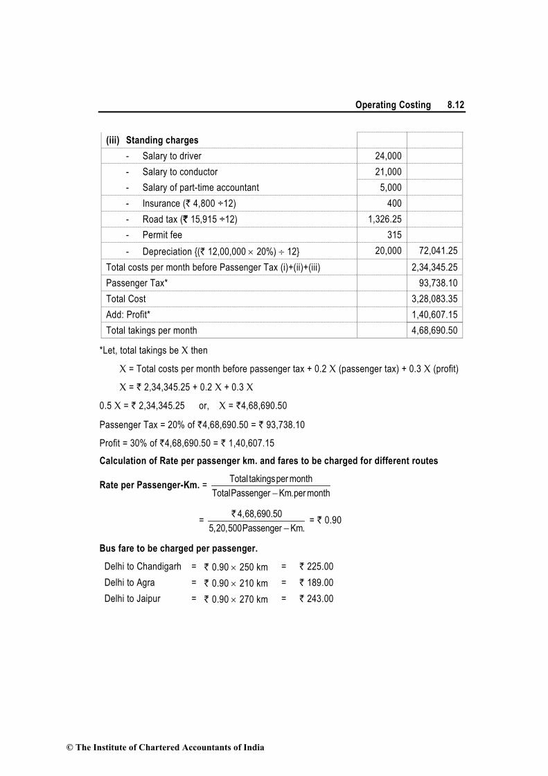
Operating Costing 8.12
(iii) Standing charges
- Salary to driver 24,000
- Salary to conductor 21,000
- Salary of part-time accountant 5,000
- Insurance (` 4,800 ÷12) 400
- Road tax (` 15,915 ÷12) 1,326.25
- Permit fee 315
- Depreciation {(` 12,00,000 × 20%) ÷ 12} 20,000 72,041.25
Total costs per month before Passenger Tax (i)+(ii)+(iii) 2,34,345.25
Passenger Tax* 93,738.10
Total Cost 3,28,083.35
Add: Profit* 1,40,607.15
Total takings per month 4,68,690.50
*Let, total takings be X then
X = Total costs per month before passenger tax + 0.2 X (passenger tax) + 0.3 X (profit)
X = ` 2,34,345.25 + 0.2 X + 0.3 X
0.5 X = ` 2,34,345.25 or, X = `4,68,690.50
Passenger Tax = 20% of `4,68,690.50 = ` 93,738.10
Profit = 30% of `4,68,690.50 = ` 1,40,607.15
Calculation of Rate per passenger km. and fares to be charged for different routes
Rate per Passenger-Km. = Total takingsper month
TotalPassenger Km.per month−
= 4,68,690.50
5,20,500Passenger Km.−`
= ` 0.90
Bus fare to be charged per passenger.
Delhi to Chandigarh = ` 0.90 × 250 km = ` 225.00
Delhi to Agra = ` 0.90 × 210 km = ` 189.00
Delhi to Jaipur = ` 0.90 × 270 km = ` 243.00
© The Institute of Chartered Accountants of India

8.13 Cost Accounting
Illustration 6 (Evaluation of conveyance facilities)
A company is considering three alternative proposals for conveyance facilities for its sales
personnel who has to do considerable traveling, approximately 20,000 kilometres every year.
The proposals are as follows:
(i) Purchase and maintain its own fleet of cars. The average cost of a car is ` 6,00,000.
(ii) Allow the Executive use his own car and reimburse expenses at the rate of ` 10 per
kilometer and also bear insurance costs.
(iii) Hire cars from an agency at ` 1,80,000 per year per car. The company will have to bear
costs of petrol, taxes and tyres.
The following further details are available:
Petrol `6 per km. Repairs and maintenance `0.20 per km.
Tyre `0.12 per km. Insurance ` 1,200 per car per annum
Taxes ` 800 per car per annum Life of the car: 5 years with annual mileage of 20,000 km.
Resale value: ` 80,000 at the end of the fifth year.
Work out the relative costs of three proposals and rank them.
Solution:
Calculation of relative costs of three proposals and their ranking
I
Use of company’s car
II
Use of own car
III
Use of hired car
per annum (`)
per km. (`) per km. (`) per km. (`)
Reimbursement -- 10.00 9.00*
Fixed cost:
Insurance 1,200 0.06 0.06 --
Taxes 800 0.04 -- 0.04
Depreciation
(` 6,00,000 - `80,000) ÷ 5 year
1,04,000 5.20 -- --
© The Institute of Chartered Accountants of India

Operating Costing 8.14
Running and Maintenance Cost:
Petrol -- 6.00 -- 6.00
Repairs and Maintenance -- 0.20 -- --
Tyre -- 0.12 -- 0.12
Total cost per km. -- 11.62 10.06 15.16
Cost for 20,000 km. 2,32,400 2,01,200 3,03,200
Ranking of proposals II I III
* (` 1,80,000 ÷ 20,000 km.)
The Second alternative i.e., use of own car by the executive and reimbursement of expenses
by the company is the best alternative from company’s point of view.
Illustration 7 (Calculation of cost of per kWh by a power generation company)
From the following data pertaining to the year 2014-15 prepare a cost statement showing the
cost of electricity generated per kwh by Chambal Thermal Power Station.
Total units generated 10,00,000 kwh
(`)
Operating labour 15,00,000
Repairs & maintenance 5,00,000
Lubricants, spares and stores 4,00,000
Plant supervision 3,00,000
Administration overheads 20,00,000
5 kwh. of electricity generated per kg. of coal consumed @` 4.25 per kg. Depreciation
charges @ 5% on capital cost of ` 2,00,00,000.
Solution
Cost Statement of Chambal Thermal Power Station
Total units generated 10,00,000 kwh.
Per annum (`) Per k.w.h. (`)
Fixed costs :
Plant supervision 3,00,000
Administration overheads 20,00,000
Depreciation (5% of ` 2,00,00,000 p.a.) 10,00,000
Total fixed cost: (A) 33,00,000 3.30
© The Institute of Chartered Accountants of India

8.15 Cost Accounting
Variable costs:
Operating labour 15,00,000
Lubricants, spares and stores 4,00,000
Repairs & maintenance 5,00,000
Coal cost (Refer to working note) 8,50,000
Total variable cost: (B) 32,50,000 3.25
Total cost [(A) + (B)] 65,50,000 6.55
Working Note:
Coal cost (10,00,000 kwh. ÷ 5 kwh) × ` 4.25 per kg. = ` 8,50,000
8.4 Standard Load
An alternative unit for the distribution of transport cost is the ‘standard load’. Where the goods
to be transported are of varying bulk and weight, the calculation of actual number of tonne-
kilometres is not an easy matter. For example, if a business delivers its own products by its
own transport, the cost per tonne-kilometres may be most misleading, for an article may have
a bulk which is twice that of the other, though of the same weight. In such a case ‘standard
load’ is selected as the unit, i.e., the load which a lorry would carry. This would have reference
both to bulk and weight and would give an efficient method for distributing the cost of transport
over different departments. Thus, if the turnover of various departments is reduced to
‘standard load’ by first calculating their weight and then the bulk of article produced, the costs
of distributing the product would be easily ascertained.
This principle also can be extended for associating cost with convenient units of service
rendered by an organisation so that management is able to judge whether the organisation is
running efficiently and in the manner in which the service requires to be improved or be made
more economical. The cost of generation of electricity on the same principle is correlated with
units generated and also with units sold; in hospitals the cost of their maintenance is co-
related to units of ‘available bed-days’.
8.5 Multiple Costing
It refers to the method of costing followed by a business wherein a large variety of articles are
produced, each differing from the other both in regard to material required and process of
manufacture. In such cases, cost of each article is computed separately by using, generally,
two or more methods of costing. For instance, for ascertaining the cost of a bicycle, cost of
each part will be ascertained by using batch or job costing method and, then the cost of
assembling the parts will be ascertained by following the method of single or output costing.
© The Institute of Chartered Accountants of India

Operating Costing 8.16
8.6 Summary
Operating Costing:- Used by those undertakings which provide services rather than producing
commodities.
Cost units used in the following services undertaken as below:-
Transport service − Passenger km., quintal km., or tonne km.
Supply service − Kwh, Cubic metre, per kg., per litre.
Hospital − Patient per day, room per day or per bed, per operation etc.
Canteen − Per item, per meal etc.
Cinema − Per ticket.
© The Institute of Chartered Accountants of India

9 PROCESS & OPERATION COSTING
Learning Objectives
After studying this chapter, you should be able to
Understand the meaning of Process and Operation costing
Understand the accounting treatment required for normal and abnormal process losses
Understand the treatment for abnormal gain
Understand the treatment of inter process profit in the process accounts
9.1 Meaning of Process Costing
Process Costing is a method of costing used in industries where the material has to pass through
two or more processes for being converted into a final product. It is defined as “a method of Cost
Accounting whereby costs are charged to processes or operations and averaged over units
produced”. A separate account for each process is opened and all expenditure pertaining to a
process is charged to that process account. Such type of costing method is useful in the
manufacturing of products like steel, paper, medicines, soaps, chemicals, rubber, vegetable oil,
paints, varnish etc. where the production process is continuous and the output of one process
becomes the input of the following process till completion.
9.1.1 Basic features: Industries, where process costing can be applied, have normally one
or more of the following features:
1. Each plant or factory is divided into a number of processes, cost centres or departments,
and each such division is a stage of production or a process.
2. Manufacturing activity is carried on continuously by means of one or more process run
sequentially, selectively or simultaneously.
3. The output of one process becomes the input of another process.
4. The end product usually is of like units not distinguishable from one another.
5. It is not possible to trace the identity of any particular lot of output to any lot of input
materials. For example, in the sugar industry, it is impossible to trace any lot of sugar
bags to a particular lot of sugarcane fed or vice versa.
6. Production of a product may give rise to Joint and/or By-Products.
© The Institute of Chartered Accountants of India

9.2 Cost Accounting
9.1.2 Costing Procedure: The Cost of each process comprises the cost of :
(i) Materials (ii) Labour
(iii) Direct expenses, and (iv) Overheads of production.
Materials - Materials and supplies which are required for each process are drawn against
material requisitions from stores. Each process for which the above drawn materials will be
used should be debited with the cost of materials consumed on the basis of the information
received from the Cost Accounting department. The finished product of first process generally
become the raw materials of second process; under such a situation the account of second
process, be debited with the cost of transfer from the first process and the cost of any
additional material required under this second process.
Labour - Each process account should be debited with the labour cost or wages paid to labour
for carrying out the processing activities. Sometimes the wages paid are apportioned over the
different processes after selecting appropriate basis.
Direct expenses - Each process account should be debited with direct expenses like
depreciation, repairs, maintenance, insurance etc. associated with it.
Overheads of production - Expenses like rent, power expenses, lighting bills, gas and water
bills etc. are known as production overheads. These expenses cannot be allocated to a
process. The suitable wayout to recover them is to apportion them over different processes by
using suitable basis. Usually, these expenses are estimated in advance and the processes
debited with these expenses on a pre-determined basis.
9.2 Operation Costing
It is defined as the refinement of process costing. It is concerned with the determination of the
cost of each operation rather than the process. In those industries where a process consists of
distinct operations, the method of costing applied or used is called operation costing.
Operation costing offers better scope for control. It facilitates the computation of unit operation
cost at the end of each operation by dividing the total operation cost by total output units.
Operation costing is just a variant of unit or output costing. The expenses of operating a
service for a particular period are grouped under suitable headings and their total is divided by
the number of service units for the same period and thus cost per unit of service is obtained.
The cost for a further period may be estimated on the basis of estimated service units and the
estimated costs. This will help in fixing the price to be charged for the service units and the
estimated cost.
Illustration 1: (Preparation of process cost accounts)
From the following data, prepare process accounts indicating the cost of each process and the
total cost. The total units that pass through each process were 240 for the period.
© The Institute of Chartered Accountants of India

Process & Operation Costing 9.3
Process A (`) Process B (`) Process C (`)
Materials 1,500 500 200
Labour 800 2,000 600
Other expenses 260 720 250
Indirect expenses amounting to ` 850 may be apportioned on the basis of wages. There was
no opening or closing stock.
Solution:
Dr. Process ‘A’ Account Cr.
Particulars Per unit (`)
Total (`)
Particulars Per unit (`)
Total (`)
To Material 6.25 1,500 By Process ‘B’ A/c 11.50 2,760
” Labour 3.34 800 (Transfer to Process-B)
” Other expenses 1.08 260
” Indirect expenses* 0.83 200
11.50 2,760 11.50 2,760
Dr. Process ‘B’ Account Cr.
Particulars Per unit (`)
Total (`)
Particulars Per unit (`)
Total (`)
To Process-A A/c 11.50 2,760 By Process ‘C’ A/c 27.00 6,480
” Material 2.08 500 (Transfer to Process-C)
” Labour 8.34 2,000
” Other expenses 3.00 720
” Indirect expenses* 2.08 500
27.00 6,480 27.00 6,480
Dr. Process ‘C’ Account Cr.
Particulars Per unit (`)
Total (`)
Particulars Per unit (`)
Total (`)
To Process-B A/c 27.00 6,480 By Finished Stock A/c 32.00 7,680
Material 0.83 200 (Transferred)
” Labour 2.50 600
© The Institute of Chartered Accountants of India

9.4 Cost Accounting
” Other expenses 1.04 250
” Indirect expenses* 0.63 150
32.00 7,680 32.00 7,680
* Apportionment of Indirect expenses among Process-A, Process-B and Process-C
Total Wages to processes (A +B +C) = ` 800 + ` 2,000 + ` 600 = ` 3,400
Apportionment to:
Process- A = 850
8003,400
×`
``
= `200; Process- B = 850
2,0003,400
×`
``
= `500 and
Process- C = 850
6003,400
×`
``
= `150
9.3 Treatment of Normal Process Loss, Abnormal Process Loss And Abnormal Gain In Cost Accounting
Loss of material is inherent during processing operation. The loss of material under different
processes arises due to reasons like evaporation or a change in the moisture content etc.
Process loss is defined as the loss of material arising during the course of a processing
operation and is equal to the difference between the input quantity of the material and its
output.
There are two types of material losses viz. (i) Normal loss and (ii) Abnormal loss.
(i) Normal Process Loss: It is defined as the loss of material which is inherent in the
nature of work. Such a loss can be reasonably anticipated from the nature of the material,
nature of operation, the experience and technical data. It is unavoidable because of nature of
the material or the process. It also includes units withdrawn from the process for test or
sampling.
Treatment in Cost Accounts : The cost of normal process loss in practice is absorbed by
good units produced under the process. The amount realised by the sale of normal process
loss units should be credited to the process account.
(ii) Abnormal Process Loss: It is defined as the loss in excess of the pre-determined loss
(Normal process loss). This type of loss may occur due to the carelessness of workers, a bad
plant design or operation, sabotage etc. Such a loss cannot obviously be estimated in
advance. But it can be kept under control by taking suitable measures.
Treatment in Cost Accounts: The cost of an abnormal process loss unit is equal to the cost
of a good unit. The total cost of abnormal process loss is credited to the process account from
which it arises. Cost of abnormal process loss is not treated as a part of the cost of the
© The Institute of Chartered Accountants of India

Process & Operation Costing 9.5
product. In fact, the total cost of abnormal process loss is debited to costing profit and loss
account.
(iii) Abnormal Process Gain: Sometimes, loss under a process is less than the anticipated
normal figure. In other words, the actual production exceeds the expected figures. Under such
a situation the difference between actual and expected loss or actual and expected production
is known as abnormal gain. So abnormal gain may be defined as an unexpected gain in
production under the normal conditions.
Treatment in Cost Accounts: The process account under which abnormal gain arises is
debited with the abnormal gain and credited to abnormal gain account which will be closed by
transferring to the Costing Profit and Loss account. The cost of abnormal gain is computed on
the basis of normal production.
To be more clear about the above concepts we consider the following illustration.
Illustration 2: (Treatment of normal loss, abnormal loss and abnormal gain)
A product passes through three processes. The output of each process is treated as the raw
material of the next process to which it is transferred and output of the third process is
transferred to finished stock.
1st Process (`) 2nd Process (`) 3rd Process (`)
Materials issued 40,000 20,000 10,000
Labour 6,000 4,000 1,000
Manufacturing overhead 10,000 10,000 15,000
10,000 units have been issued to the 1st process and after processing, the output of each
process is as under:
Output Normal Loss
1st Process 9,750 units 2%
2nd Process 9,400 units 5%
3rd Process 8,000 units 10%
No stock of materials or of work-in-progress was left at the end. Calculate the cost of the
finished articles.
Solution:
Dr. 1st Process Account Cr.
Particulars Units Total (`)
Particulars Units Total (`)
To Material 10,000 40,000 By Normal Loss A/c
(2% of 10,000 units)
200 --
© The Institute of Chartered Accountants of India

9.6 Cost Accounting
” Labour -- 6,000 ” Abnormal Loss A/c
(` 5.7142 × 50 units)
50 286
” Manufacturing OH -- 10,000 ” 2nd Process A/c
(` 5.7142 × 9,750 units)
9,750 55,714
10,000 56,000 10,000 56,000
Cost per unit of completed units and abnormal loss:
TotalCost
Inputs Normal loss−=
56,000
10,000units 200units−
` = ` 5.7142
Dr. 2nd Process Account Cr.
Particulars Units Total (`)
Particulars Units Total (`)
To 1st Process A/c 9,750 55,714 By Normal Loss A/c
(5% of 9,750 units)
488 --
” Material -- 20,000 ” 3rd Process A/c
(` 9.6862 × 9,400 units)
9,400 91,051
” Labour -- 4,000
” Manufacturing OH -- 10,000
” Abnormal Gain A/c
(` 9.6862 × 138 units)
138 1,337
9,888 91,051 9,888 91,051
Cost per unit of completed units and abnormal gain:
TotalCost
Inputs Normal loss−=
89,714
9,750units 488units−
` = ` 9.6862
Dr. 3rd Process Account Cr.
Particulars Units Total
(`)
Particulars Units Total
(`)
To 2nd Process A/c 9,400 91,051 By Normal Loss A/c
(10% of 9,400 units)
940 --
” Material -- 10,000 ” Abnormal Loss A/c
(`13.8358 × 460 units)
460 6,364
© The Institute of Chartered Accountants of India

Process & Operation Costing 9.7
” Labour -- 1,000 ” Finished Stock A/c
(`13.8358 × 8,000
units)
8,000 1,10,687
” Manufacturing
OH
-- 15,000
9,400 1,17,051 9,400 1,17,051
Cost per unit of completed units and abnormal loss:
TotalCost
Inputs Normal loss−=
1,17,051
9,400units 940units−
` = `13.8358
Illustration 3 (Preparation of process accounts)
RST Limited processes Product Z through two distinct processes – Process I and Process II.
On completion, it is transferred to finished stock. From the following information for the year
2011-12, prepare Process I, Process II and Finished Stock A/c:
Particulars Process I Process II
Raw materials used 7,500 units --
Raw materials cost per unit ` 60 --
Transfer to next process/finished stock 7,050 units 6,525 units
Normal loss (on inputs) 5% 10%
Direct wages ` 1,35,750 ` 1,29,250
Direct Expenses 60% of Direct wages 65% of Direct wages
Manufacturing overheads 20% of Direct wages 15% of Direct wages
Realisable value of scrap per unit ` 12.50 ` 37.50
6,000 units of finished goods were sold at a profit of 15% on cost. Assume that there was no
opening or closing stock of work-in-progress.
Solution
Process I A/c
Particulars Units (`) Particulars Units (`)
To Raw material used
(`60 × 7,500 units)
7,500 4,50,000 By Normal loss
(5% of 7,500 units)×
`12.5
375 4,688
To Direct wages -- 1,35,750 By Process II A/c
(`96.7947 × 7,050
units)
7,050 6,82,40
3
© The Institute of Chartered Accountants of India

9.8 Cost Accounting
To Direct expenses -- 81,450 By Abnormal loss
(`96. 7947 × 75 units)
75 7,259
To Manufacturing
overhead
27,150
7,500 6,94,350 7,500 6,94,35
0
Cost per unit of completed units and abnormal loss: TotalCost Re alisable value fromnormal loss
Inputsunits Normal lossunits
−
−
=6,94,350 4,688
7,500units 375 units
−
−
` `=
6,89,662
7,125 units
`= `96.7947
Process II A/c
Particulars Units (`) Particulars Units (`)
To Process I A/c
7,050 6,82,403 By Normal loss
(10% of 7,050 units)× ` 37.5
705 26,438
To Direct wages -- 1,29,250 By Finished Stock A/c
(`140.0496 × 6,525 units)
6,525 9,13,824
To Direct expenses -- 84,013
To Manufacturing overhead -- 19,387
To Abnormal gain
(`140.0496 × 180 units)
180 25,209
7,230 9,40,262 7,230 9,40,262
Cost per unit of completed units and abnormal loss: TotalCost Re alisable value fromnormal loss
Inputsunits Normal lossunits
−
−
= 9,15,053 26,438
7,050 units 705 units
−
−
` ` =
8,88,615
6,345 units
` = `140.0496
Finished Goods Stock A/c
Particulars Units (`) Particulars Units (`)
To Process II A/c 6,525 9,13,824 By Cost of Sales
(`140.0496 × 6,000 units)
6,000 8,40,298
By Balance c/d 525 73,526
6,525 9,13,824 6,525 9,13,824
© The Institute of Chartered Accountants of India

Process & Operation Costing 9.9
Income Statement
Particulars (`) Particulars (`)
To Cost of sales
(`140.0496 × 6,000 units)
8,40,298 By Abnormal gain
{180 units × (`140.0496 – `37.50)}
18,459
To Abnormal loss
{75 units × (`96.7947 – `12.50)}
6,322 By Sales (`8,40,298 × 115%) 9,66,343
To Net Profit 1,38,182
9,84,802 9,84,802
9.4 Costing of Equivalent Production Units
In the case of process type of industries, it is possible to determine the average cost per unit by
dividing the total cost incurred during a given period of time by the total number of units
produced during the same period. But this is hardly the case in most of the process type
industries where manufacturing is a continuous activity. The reason is that the cost incurred in
such industries represents the cost of work carried on opening work-in-progress, closing work-in-
progress and completed units. Thus to ascertain the cost of each completed unit it is necessary
to ascertain the cost of work-in-progress in the beginning and at the end of the process.
The valuation of work-in-progress presents a good deal of difficulty because it has units under
different stages of completion from those in which work has just begun to those which are only
a step short of completion. Work-in-progress can be valued on actual basis, i.e., materials
used on the unfinished units and the actual amount of labour expenses involved. However, the
degree of accuracy in such a case cannot be satisfactory. An alternative method is based on
converting partly finished units into equivalent finished units.
Equivalent production means converting the incomplete production units into their equivalent
completed units. Under each process, an estimate is made of the percentage completion of
work-in-progress with regard to different elements of costs, viz., material, labour and
overheads. It is important that the estimate of percentage of completion should be as accurate
as possible. The formula for computing equivalent completed units is:
Equivalent completed units = Actualnumber of units in Percentage of
theprocessof manufacture Work completed
×
For instance, if 25% of work has been done on the average of units still under process, then
200 such units will be equal to 50 completed units and the cost of work-in-progress will be
equal to the cost of 50 finished units.
9.4.1 Valuation of work-in-progress: For the valuation of work-in-progress following
three methods are available :
© The Institute of Chartered Accountants of India

9.10 Cost Accounting
a. First-in-First Out (FIFO) method.
b. Last-in-First Out (LIFO) method.
c. Average Cost method (or weighted average cost method).
(1) First-in-first-out method: Under this method the units completed and transferred
include completed units of opening work-in-progress and subsequently introduced units.
Proportionate cost to complete the opening work-in-progress and that to process the
completely processed units during the period are derived separately. The cost of opening
work-in-progress is added to the proportionate cost incurred on completing the same to get the
complete cost of such units. Complete cost of such units plus cost of units completely
processed constitute the total cost of units transferred. In this method the closing stock of
Work in progress is valued at current cost.
Illustration 4: (Computation of equivalent production and cost per equivalent unit under
FIFO method)
Opening work-in-progress 1,000 units (60% complete); Cost ` 1,100. Units introduced during
the period 10,000 units; Cost ` 19,300. Transferred to next process - 9,000 units.
Closing work-in-progress - 800 units (75% complete). Normal loss is estimated at 10% of total
input including units in process at the beginning. Scrap realise `1 per unit. Scraps are 100%
complete.
Compute equivalent production and cost per equivalent unit. Also evaluate the output.
Solution:
Statement of Equivalent Production Units (Under FIFO Method)
Particulars Input units
Particulars Output units
Equivalent Production
(%) Equivalent units
Opening W-I-P 1,000 From opening W-I-P 1,000 40 400
Units introduced 10,000 From fresh inputs 8,000 100 8,000
Units completed
(Transferred to next process)
9,000
Normal Loss
{10% (1,000 + 10,000 units)}
1,100 -- --
Closing W-I-P 800 75 600
Abnormal loss
(Balancing figure)
100 100 100
11,000 11,000 9,100
© The Institute of Chartered Accountants of India

Process & Operation Costing 9.11
Computation of cost per equivalent production unit :
Cost of the Process (for the period) `19,300
Less: Scrap value of normal loss (` 1 × 1,100 units) (`1,100)
Total process cost ` 18,200
Cost per equivalent unit = 18,200
9,100units
` = ` 2
Statement of Evaluation
Particulars Equivalent Units (EU)
Cost per EU (`)
Amount
(`)
(i) Opening W-I-P completed 400 2.00 800
Add: Cost of W-I-P -- -- 1,100
Complete cost of 1,000 units of opening W-I-P 1,000 1.90 1,900
(ii) Completely processes units 8,000 2.00 16,000
(iii) Abnormal Loss 100 2.00 200
(iv) Closing W-I-P 600 2.00 1,200
(2) Last-in first-out Method: According to this method units lastly entering in the process
are the first to be completed. This assumption has a different impact on the costs of the
completed units and the closing inventory of work-in-progress. The completed units will be
shown at their current cost and the closing inventory of work-in-progress will continue to
appear at the cost of the opening inventory of work-in-progress.
It may be noted that Last in First out (LIFO) is not permitted under Accounting Standard (AS)-
2: Valuation of Inventories. However for the purpose of academic knowledge LIFO method is
included in this Study Material
Illustration 5: (Computation of equivalent production and cost per equivalent unit under
LIFO method)
From the following information relating to the month of April 2015, calculate the equivalent
production units and the value of finished production and work-in-progress, using the LIFO method.
Opening work-in-progress on 1st April: 5,000 units; 50% complete.
Cost (`)
Materials 6,000
Labour 8,000
Overheads 8,000
22,000
© The Institute of Chartered Accountants of India

9.12 Cost Accounting
Units introduced into the process : 10,000.
Cost (`)
Materials 30,000
Labour 52,500
Overheads 70,000
1,52,500
During the period 7,500 units were completed and transferred to the next process. Closing
work-in-progress on 30th April: 7,500 units, 50% complete.
Solution:
(i) Statement of Equivalent Production Units (Under LIFO Method)
Particulars Input
units
Particulars Output
units
Equivalent
Production
(%) Equivalent
units
Opening W-I-P 5,000 From fresh units
(Units completed and
transferred to next
process)
7,500 100 7,500
Units introduced 10,000 Closing W-I-P:
- From fresh units 2,500 50 1,250
- From Opening W-I-
P*
5,000 -- --
15,000 15,000 8,750
* Since the units in the opening work in process were already 50% complete; no work has been done on these units during the period.
(ii) Cost per unit of equivalent production = 1,52,500
8,750units
` =` 17.43
Valuation of finished production and WIP:
1. Finished Production (7,500 units × ` 17.43) ` 1,30,725.00
2. Closing W-I-P {` 22,000 + (1,250 units × `17.43)} ` 43,787.50
(3) Average Cost Method : Under this method, the cost of opening work-in-progress and
cost of the current period are aggregated and the aggregate cost is divided by output in terms
of completed units. The equivalent production in this case consists of work-load already
contained in opening work-in-process and work-load of current period.
© The Institute of Chartered Accountants of India

Process & Operation Costing 9.13
The main difference between FIFO method and average method is that units of opening work
in progress and their cost are taken in full under average method while under FIFO method
only the remaining work done now is considered.
Illustration 6: (Computation of equivalent production and cost per equivalent unit under
Average cost method)
Refer to information provided in Illustration 4 above and solve this by Average Cost Method.
Solution:
Statement of Equivalent Production Units (Under Average Cost Method)
Particulars Input
units
Particulars Outpu
t units
Equivalent
Production
(%) Equivalen
t units
Opening W-I-P 1,000 Units completed
(Transferred to next
process)
9,000 100 9,000
Units introduced 10,000 Normal Loss
{10% (1,000 + 10,000
units)}
1,100 -- --
Closing W-I-P 800 75 600
Abnormal loss
(Balancing figure)
100 100 100
11,000 11,000 9,700
Computation of cost per equivalent production unit :
Cost of Opening W-I-P ` 1,100
Cost of the Process (for the period) `19,300
Less: Scrap value of normal loss (` 1 × 1,100 units) (`1,100)
Total process cost ` 19,300
Cost per equivalent unit = 19,300
9,700units
` = ` 1.99
Statement of Evaluation
Particulars Equivalent Units (EU)
Cost per EU
(`)
Amount
(`)
(i) Units Completed and transferred to next process 9,000 1.99 17,910
© The Institute of Chartered Accountants of India

9.14 Cost Accounting
(ii) Abnormal Loss 100 1.99 199
(iii) Closing W-I-P 600 1.99 1,194
Illustration 7: (Computation of equivalent production and cost per equivalent unit under
Average cost method)
Following information is available regarding process A for the month of February, 2015 :
Production Record:
Units in process as on 1.2.2015
(All materials used, 25% complete for labour and overhead)
4,000
New units introduced 16,000
Units completed 14,000
Units in process as on 28.2.2015
(All materials used, 33-1/3% complete for labour and overhead)
6,000
Cost Records:
Work-in-process as on 1.2.2015 (`)
Materials 6,000
Labour 1,000
Overhead 1,000
8,000
Cost during the month
Materials 25,600
Labour 15,000
Overhead 15,000
55,600
Presuming that average method of inventory is used, prepare:
(i) Statement of equivalent production.
(ii) Statement showing cost for each element.
(iii) Statement of apportionment of cost.
(iv) Process cost account for Process A.
Solution
(i) Statement of equivalent production (Average cost method)
Particulars Input
Units
Particulars Output
Units
Equivalent Production
Material Labour & O.H.
% Units % Units
Opening WIP 4,000 Completed and
transferred
14,000 100 14,000 100 14,000
© The Institute of Chartered Accountants of India
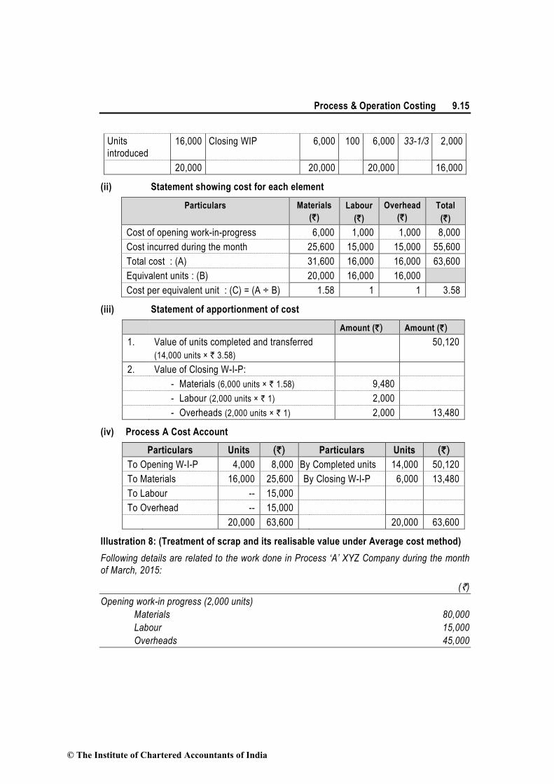
Process & Operation Costing 9.15
Units
introduced
16,000 Closing WIP 6,000 100 6,000 33-1/3 2,000
20,000 20,000 20,000 16,000
(ii) Statement showing cost for each element
Particulars Materials
(`)
Labour
(`)
Overhead
(`)
Total
(`)
Cost of opening work-in-progress 6,000 1,000 1,000 8,000
Cost incurred during the month 25,600 15,000 15,000 55,600
Total cost : (A) 31,600 16,000 16,000 63,600
Equivalent units : (B) 20,000 16,000 16,000
Cost per equivalent unit : (C) = (A ÷ B) 1.58 1 1 3.58
(iii) Statement of apportionment of cost
Amount (`) Amount (`)
1. Value of units completed and transferred
(14,000 units × ` 3.58)
50,120
2. Value of Closing W-I-P:
- Materials (6,000 units × ` 1.58) 9,480
- Labour (2,000 units × ` 1) 2,000
- Overheads (2,000 units × ` 1) 2,000 13,480
(iv) Process A Cost Account
Particulars Units (`) Particulars Units (`)
To Opening W-I-P 4,000 8,000 By Completed units 14,000 50,120
To Materials 16,000 25,600 By Closing W-I-P 6,000 13,480
To Labour -- 15,000
To Overhead -- 15,000
20,000 63,600 20,000 63,600
Illustration 8: (Treatment of scrap and its realisable value under Average cost method)
Following details are related to the work done in Process ‘A’ XYZ Company during the month
of March, 2015:
(`)
Opening work-in progress (2,000 units)
Materials 80,000
Labour 15,000
Overheads 45,000
© The Institute of Chartered Accountants of India

9.16 Cost Accounting
Materials introduced in Process ‘A’ (38,000 units) 14,80,000
Direct Labour 3,59,000
Overheads 10,77,000
Units scrapped : 3,000 units
Degree of completion :
Materials 100%
Labour and overheads 80%
Closing work-in progress : 2,000 units
Degree of completion :
Materials 100%
Labour and overheads 80%
Units finished and transferred to Process ‘B’ : 35,000 units
Normal Loss :
5% of total input including opening work-in-progress.
Scrapped units fetch ` 20 per piece.
You are required to prepare :
(i) Statement of equivalent production
(ii) Statement of cost
(iii) Statement of distribution cost, and
(iv) Process ‘A’ Account, Normal Loss Account and Abnormal Loss Account.
Solution
(i) Statement of Equivalent Production
Particulars Input Units
Particulars Output Units
Equivalent Production
Material Labour & O.H.
% Units % Units
Opening WIP 2,000 Completed and transferred to Process B
35,000 100 35,000 100 35,000
Units introduced 38,000 Normal Loss (5% of 40,000) 2,000 -- -- -- --
Abnormal loss
(Balancing figure)
1,000 100 1,000 80 800
Closing WIP 2,000 100 2,000 80 1,600
40,000 40,000 38,000 37,400
© The Institute of Chartered Accountants of India

Process & Operation Costing 9.17
(ii) Statement showing cost for each element
Particulars Materials
(`)
Labour
(`)
Overhead
(`)
Total
(`)
Cost of opening work-in-progress 80,000 15,000 45,000 1,40,000
Cost incurred during the month 14,80,000 3,59,000 10,77,000 29,16,000
Less: Realisable Value of normal
scrap
(` 20 × 2,000 units)
(40,000) -- -- (40,000)
Total cost : (A) 15,20,000 3,74,000 11,22,000 30,16,000
Equivalent units : (B) 38,000 37,400 37,400
Cost per equivalent unit : (C) =
(A ÷ B)
40.00 10.00 30.0 80.00
(iii) Statement of Distribution of cost
Amount (`) Amount (`)
1. Value of units completed and transferred
(35,000 units × ` 80)
28,00,000
2. Value of Abnormal Loss:
- Materials (1,000 units × ` 40) 40,000
- Labour (800 units × ` 10) 8,000
- Overheads (800 units × ` 30) 24,000 72,000
3. Value of Closing W-I-P:
- Materials (2,000 units × ` 40) 80,000
- Labour (1,600 units × ` 10) 16,000
- Overheads (1,600 units × ` 30) 48,000 1,44,000
(iv) Process A A/c
Particulars Units (`) Particulars Units (`)
To Opening W.I.P: By Normal Loss
(`20 × 2,000 units)
2,000 40,000
- Materials 2,000 80,000 By Abnormal loss 1,000 72,000
- Labour -- 15,000 By Process B A/c 35,000 28,00,000
- Overheads -- 45,000 By Closing WIP 2,000 1,44,000
To Materials introduced
38,000 14,80,000
© The Institute of Chartered Accountants of India

9.18 Cost Accounting
To Direct Labour 3,59,000
To Overheads 10,77,000
40,000 30,56,000 40,000 30,56,000
Normal Loss A/c
Particulars Units (`) Particulars Units (`)
To Process A A/c 2,000 40,000 By Cost Ledger Control A/c 2,000 40,000
2,000 40,000 2,000 40,000
Abnormal Loss A/c
Particulars Units (`) Particulars Units (`)
To Process A A/c 1,000 72,000 By Cost Ledger Control A/c 1,000 20,000
By Costing Profit & Loss A/c 52,000
1,000 72,000 1,000 72,000
Illustration 9: (Preparation of statement of equivalent production)
A company produces a component, which passes through two processes. During the month of
April, 2015, materials for 40,000 components were put into Process I of which 30,000 were
completed and transferred to Process II. Those not transferred to Process II were 100%
complete as to materials cost and 50% complete as to labour and overheads cost. The
Process I costs incurred were as follows :
Direct material `15,000
Direct wages `18,000
Factory overheads `12,000
Of those transferred to Process II, 28,000 units were completed and transferred to finished
goods stores. There was a normal loss with no salvage value of 200 units in Process II. There
were 1,800 units, remained unfinished in the process with 100% complete as to materials and
25% complete as regard to wages and overheads.
No further process material costs occur after introduction at the first process until the end of
the second process, when protective packing is applied to the completed components. The
process and packing costs incurred at the end of the Process II were :
Packing materials `4,000
Direct wages `3,500
Factory overheads `4,500
© The Institute of Chartered Accountants of India

Process & Operation Costing 9.19
Required :
(i) Prepare Statement of Equivalent Production, Cost per unit and Process I A/c.
(ii) Prepare Statement of Equivalent Production, Cost per unit and Process II A/c.
Solution: (i) Process I – Statement of Equivalent Production
Particulars Completed
Units
Closing stock of WIP Equivalent
Production units
Units % of
Completion
Equivalent
Units
(1) (2) (1) + (2)
Material 30,000 10,000 100% 10,000 40,000
Wages 30,000 10,000 50% 5,000 35,000
Overhead 30,000 10,000 50% 5,000 35,000
Process I
Particulars Process Cost
(`)
Equivalent
Production (units)
Process Cost p.u.
(2)/(3)
WIP stock
Equivalent
units
Cost of WIP
Stock (`)
(4) × (5)
Transfer to
Process II (2)-(6)
(1) (2) (3) (4) (5) (6) (7)
Material 15,000 40,000 0.375 10,000 3,750 11,250
Wages 18,000 35,000 0.514 5,000 2,570 15,430
Overhead 12,000 35,000 0.343 5,000 1,715 10,285
45,000 8,035 36,965
Process I A/c
Particulars Unit (`) Particulars Units (`)
To Direct material 40,000 15,000 By Process II A/c 30,000 36,965
To Direct wages -- 18,000 By Closing W-I-P 10,000 8,035
To Factory overhead -- 12,000 -- --
40,000 45,000 40,000 45,000
© The Institute of Chartered Accountants of India

9.20 Cost Accounting
(ii) Process II – Statement of Equivalent Production
Particulars Completed
Units
Closing stock of WIP Equivalent
Production units
Units % of
Completion
Equivalent
Units
(1) (2) (1) + (2)
Material 28,000 1,800 100% 1,800 29,800
Wages 28,000 1,800 25% 450 28,450
Overhead 28,000 1,800 25% 450 28,450
Process II
Particulars Process Cost
(`)
Equivalent
Production (units)
Process Cost p.u.
(2)/(3)
WIP stock
Equivalent
units
Cost of WIP Stock
(`)
(4)× (5)
Transfer to
Finished Stock
(2)-(6)
(1) (2) (3) (4) (5) (6) (7)
Material 36,965 29,800 1.240 1,800 2,232 34,733
Wages 3,500 28,450 0.123 450 55 3,445
Overhead 4,500 28,450 0.158 450 71 4,429
44,965 2,358 42,607
Add: Packing Material Cost 4,000
Cost of Finished Stock 46,607
Process II A/c
Particulars Units (`) Particulars Units (`)
To Process I 30,000 36,965 By Finished
Stock
28,000 46,607
To Direct wages -- 3,500 By Normal loss 200 --
To Factory
overhead -- 4,500 By WIP stock 1,800 2,358
To Packing charges -- 4,000
30,000 48,965 30,000 48,965
© The Institute of Chartered Accountants of India

Process & Operation Costing 9.21
9.5 Inter-Process Profits
In some process industries the output of one process is transferred to the next process not at
cost but at market value or cost plus a percentage of profit. The difference between cost and
the transfer price is known as inter-process profits.
The advantages and disadvantages of using inter-process profit, in the case of process type
industries are as follows:
Advantages:
1. Comparison between the cost of output and its market price at the stage of completion is
facilitated.
2. Each process is made to stand by itself as to the profitability.
Disadvantages:
1. The use of inter-process profits involves complication.
2. The system shows profits which are not realised because of stock not sold out.
Illustration 10: (Preparation of process cost accounts with inter process profit)
A Ltd. produces product ‘AXE’ which passes through two processes before it is completed and
transferred to finished stock. The following data relate to October 2014 :
Process I (`)
Process II (`)
Finished Stock (`)
Opening stock 7,500 9,000 22,500
Direct materials 15,000 15,750 --
Direct wages 11,200 11,250 --
Factory overheads 10,500 4,500 --
Closing stock 3,700 4,500 11,250
Inter-process profit included in opening stock -- 1,500 8,250
Output of Process I is transferred to Process II at 25% profit on the transfer price.
Output of Process II is transferred to finished stock at 20% profit on the transfer price. Stock in
process is valued at prime cost. Finished stock is valued at the price at which it is received
from process II. Sales during the period are ` 1,40,000.
Prepare Process cost accounts and finished goods account showing the profit element at each
stage.
© The Institute of Chartered Accountants of India
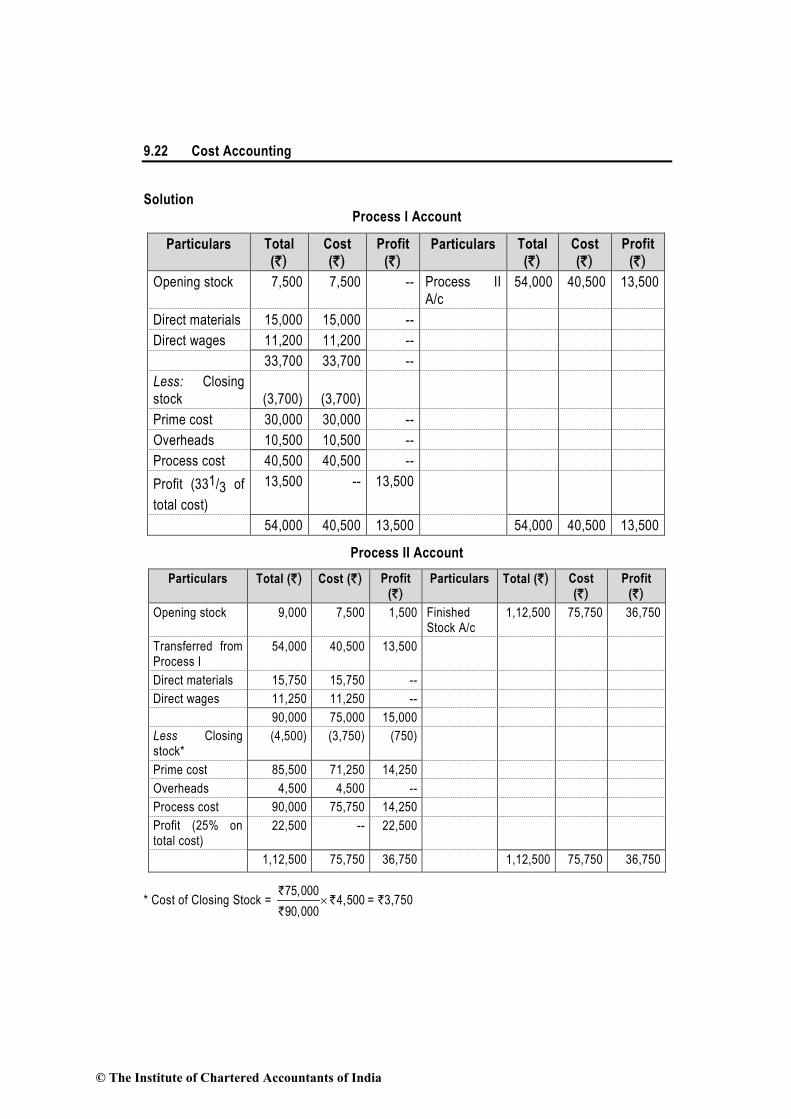
9.22 Cost Accounting
Solution
Process I Account
Particulars Total
(`)
Cost
(`)
Profit
(`)
Particulars Total
(`)
Cost
(`)
Profit
(`)
Opening stock 7,500 7,500 -- Process II
A/c
54,000 40,500 13,500
Direct materials 15,000 15,000 --
Direct wages 11,200 11,200 --
33,700 33,700 --
Less: Closing
stock
(3,700)
(3,700)
Prime cost 30,000 30,000 --
Overheads 10,500 10,500 --
Process cost 40,500 40,500 --
Profit (331/3 of
total cost)
13,500 -- 13,500
54,000 40,500 13,500 54,000 40,500 13,500
Process II Account
Particulars Total (`) Cost (`) Profit (`)
Particulars Total (`) Cost (`)
Profit (`)
Opening stock 9,000 7,500 1,500 Finished Stock A/c
1,12,500 75,750 36,750
Transferred from Process I
54,000 40,500 13,500
Direct materials 15,750 15,750 --
Direct wages 11,250 11,250 --
90,000 75,000 15,000
Less Closing stock*
(4,500) (3,750) (750)
Prime cost 85,500 71,250 14,250
Overheads 4,500 4,500 --
Process cost 90,000 75,750 14,250
Profit (25% on total cost)
22,500 -- 22,500
1,12,500 75,750 36,750 1,12,500 75,750 36,750
* Cost of Closing Stock = 75,000
4,50090,000
×`
``
= `3,750
© The Institute of Chartered Accountants of India

Process & Operation Costing 9.23
Finished Stock Account
Particulars Total (`)
Cost (`)
Profit (`)
Particulars Total (`) Cost (`)
Profit (`)
Opening
stock
22,500 14,250 8,250 Process II
A/c
1,40,000 82,500 57,500
Process II 1,12,500 75,750 36,750
1,35,000 90,000 45,000
Less: Closing
stock*
(11,250) (7,500) (3,750)
Finished
stock
1,23,750 82,500 41,250
Profit 16,250 -- 16,250
1,40,000 82,500 57,500 1,40,000 82,500 57,500
* Cost of Closing Stock = 90,000
11,2501,35,000
×`
``
= `7,500
Working Notes:
Let the transfer price be 100 then profit is 25; i.e. cost price is `75.
1. If cost is ` 75 then profit is ` 25
If cost is ` 40,500 then profit is 75
25× 40,500 = ` 13,500
2. If cost is ` 80 then profit is ` 20
If cost is ` 90,000 then profit is 80
20× 90,000 = ` 22,500
9.6 Summary
Process Costing:- Used in industries where the material has to pass through two or more
processes for being converted into a final product.
Operation Costing:- It is the refinement of process costing. It is concerned with the
determination of the cost of each operation rather than the process.
Treatment of Losses in process costing:-
© The Institute of Chartered Accountants of India

9.24 Cost Accounting
(i) Normal process loss - The cost of normal process loss is absorbed by good units
produced under the process. The amount realised by the sale of normal process loss units
should be credited to the process account.
(ii) Abnormal process loss - The total cost of abnormal process loss is credited to the
process account from which it arises. The total cost of abnormal process loss is debited to
costing profit and loss account.
Abnormal gain- The process account under which abnormal gain arises is debited with the
abnormal gain and credited to Abnormal gain account which will be closed by transferring to
the Costing Profit and loss account.
Equivalent production units: This concept is used in the industries where manufacturing is a
continuous activity. Converting partly finished units into equivalent finished units.
Equivalent production means converting the incomplete production units into their
equivalent completed units.
Equivalent completed units = {Actual number of units in the process of manufacture} ×
{Percentage of work completed}
Valuation of work-in-progress : three methods :
(1) First-in-First Out (FIFO) method.
(2) Last-in-First Out (LIFO) method.
(3) Average Cost method (or weighted average cost method).
Inter-Process Profits
The output of one process is transferred to the next process not at cost but at market value or
cost plus a percentage of profit. The difference between cost and the transfer price is known
as inter-process profits.
© The Institute of Chartered Accountants of India

10 Joint Products & By Products
Learning Objectives
After studying this chapter, you should be able to
Understand and differentiate between Joint and By products
Understand the different methods joint cost apportionment over joint products
Understand the different methods joint cost apportionment over by-products
Understand the accounting treatment required for joint products and by products
10.1 Meaning of Joint Products and By-Products
Agricultural product industries, chemical process industries, sugar industries, and extractive
industries are some of the industries where two or more products of equal or unequal
importance are produced either simultaneously or in the course of processing operation of a
main product.
In all such industries, the management is faced with the problems such as, valuation of
inventory, pricing of product and income determination, problem of taking decision in matters
of further processing of by-products and/or joint products after a certain stage etc. In fact the
various problems relate to
(i) apportionment of common costs incurred for various products and
(ii) aspects other than mere apportionment of costs incurred upto the point of separation.
Before taking up the above problems, we first define the various necessary concepts.
Joint Products - Joint products represent “two or more products separated in the course of
the same processing operation usually requiring further processing, each product being in
such proportion that no single product can be designated as a major product”.
In other words, two or more products of equal importance, produced, simultaneously from the
same process, with each having a significant relative sale value are known as joint products.
For example, in the oil industry, gasoline, fuel oil, lubricants, paraffin, coal tar, asphalt and
kerosene are all produced from crude petroleum. These are known as joint products.
© The Institute of Chartered Accountants of India

10.2 Cost Accounting
Co-Products - Joint products and co-products are used synonymously in common parlance,
but strictly speaking a distinction can be made between two. Co-products may be defined as
two or more products which are contemporary but do not emerge necessarily from the same
material in the same process. For instance, wheat and gram produced in two separate farms
with separate processing of cultivation are the co-products. Similarly timber boards made from
different trees are co-products.
By-Products - These are defined as “products recovered from material discarded in a main
process, or from the production of some major products, where the material value is to be
considered at the time of severance from the main product.” Thus by-products emerge as a
result of processing operation of another product or they are produced from the scrap or waste
of materials of a process. In short a by-product is a secondary or subsidiary product which
emanates as a result of manufacture of the main product.
The point at which they are separated from the main product or products is known as split-off
point. The expenses of processing are joint till the split –off point.
Examples of by-products are molasses in the manufacture of sugar, tar, ammonia and benzole
obtained on carbonisation of coal and glycerin obtained in the manufacture of soap.
Distinction between Joint-Product and By-Product - The main points of distinction as
apparent from the definitions of Joint Products and By-Products are:
a) Joint products are of equal importance whereas by-products are of small economic value.
b) Joint products are produced simultaneously but the by-products are produced inciden-
tally in addition to the main products.
10.2 Apportionment of joint costs
Joint product costs occur in many industries such as petroleum, oil refinery, meat-making,
textiles, dairy, flour mill, saw mill and many other process industries and top management of
business concerns require the accountants to give their opinion for many managerial decisions
such as to process further or to sell at split-off stage. To answer this question they require
apportionment of joint costs over different products produced.
The main problem faced in the case of joint products/ by-products is the apportionment of the
total cost incurred upto the point of separation of joint products/ or by products. For costs
incurred after the split off point there is no problem, as these costs can be directly allocated to
individual joint products or by-products. Thus the apportionment of joint costs over different
products produced involve the following two cases.
1. When two or more products are simultaneously produced and there is by-product.
2. When there are both joint products and by-products.
10.3 Method of apportioning joint cost over joint products
Proper apportionment of joint cost over the joint products is of considerable importance, as
© The Institute of Chartered Accountants of India

Joint Products & By-Products 10.3
this affects (a) Valuation of closing inventory; (b) Pricing of products; and (c) Profit or loss on
the sale of different products.
The commonly used methods for apportioning total process costs upto the point of separation
over the joint products are as follows:
(i) Physical unit method
(ii) Average unit cost method
(iii) Survey method
(iv) Contribution margin method
(v) Market value method :
(a) At the point of separation
(b) After further processing
(c) Net realisable value.
(i) Physical Unit Method: This method is based on the assumption that the joint products
are capable of being measured in the same units. Accordingly joint costs here are apportioned
on the basis of some physical base, such as weight or measure expressed in gallons, tonnes
etc. In other words, the basis used for apportioning joint cost over the joint products is the
physical volume of material present in the joint products at the point of separation. Any loss
arising during the stage of processing is also apportioned over the products on the same
basis. This method cannot be applied if the physical units of the two joint products are
different. The main defect of this method is that it gives equal importance and value to all the
joint products.
Illustration 1: (Apportionment of joint costs on the basis of physical unit method)
A coke manufacturing company produces the following products by using 5,000 tonnes of coal
@ ` 15 per tonne into a common process.
Coke 3,500 tonnes
Tar 1,200 tonnes
Sulphate of ammonia 52 tonnes
Benzol 48 tonnes
Apportion the joint cost amongst the products on the basis of the physical unit method.
Solution:
Products
Coke Tar Sulphate Benzol Wastage Total
of
Ammonia
Output (in tonnes) 3,500 1,200 52 48 200 5,000
Wastage (in tonnes) 146 50 2 2 200
© The Institute of Chartered Accountants of India

10.4 Cost Accounting
(apportioned on the basis of weights)
Total weight (in tonnes) 3,646 1,250 54 50 5,000
Joint Cost (in `) @ ` 15 per tonne 54,690 18,750 810 750 75,000
Note : 1. Apportionment of wastage of 200 tonnes over the four products is as follows:
Coke : 200
4,800× 3,500 tonnes = 146 tonnes
Tar : 200
4,800× 1,200 tonnes = 50 tonnes
Sulphate of ammonia : 52
4,800× 3,500 tonnes = 2 tonnes
Benzol : 48
4,800× 3,500 tonnes = 2 tonnes
(ii) Average Unit Cost Method: Under this method, total process cost (upto the point of
separation) is divided by total units of joint products produced. On division average cost per
unit of production is obtained.
Average unit cost = Total process cost (upto the point of separation) ÷ Total units of joint
product produced.
This is a simple method. The effect of application of this method is that all joint products will
have uniform cost per unit. If this method is used as the basis for price fixation, then all the
products may have more or less the same price. Under this method customers of high quality
items are benefitted as they have to pay less price on their purchase.
Illustration 2 (Apportionment of joint costs on the basis of average unit cost method)
Find out the cost of joint products A, B and C using average unit cost method from the
following data :
(a) Pre-separation Joint Cost ` 60,000
(b) Production data :
Products Units produced
A 500
B 200
C 300
1,000
Solution:
Average cost per unit =produced Units
costsjoint Total=
`
60,000
1,000 units = ` 60
© The Institute of Chartered Accountants of India

Joint Products & By-Products 10.5
The joint costs apportioned @ ` 60 are as follows :
Products Units Costs per unit (`) Value (`)
A 500 60 30,000
B 200 60 12,000
C 300 60 18,000 60,000
(iii) Survey Method: This method is also known as point value method. It is based on
technical survey of all the factors involved in the production and distribution of products. Under
this method joint cost are apportioned over the joint products, on the basis of percentage/
point values, assigned to the products according to their relative importance. The percentage
or points used for the purpose are usually computed by management with the help of technical
advisers. This method is considered to be more equitable than other methods.
(iv) Contribution Margin Method: According to this method, joint costs are segregated into two parts - variable and fixed. The variable costs are apportioned over the joint products on the basis of units produced (average method) or physical quantities. In case the products are further processed after the point of separation, then all variable cost incurred be added to the variable costs determined earlier. In this way total variable cost is arrived which is deducted from their respective sales values to ascertain their contribution. The fixed costs are then apportioned over the joint products on the basis of the contribution ratios.
Illustration 3 (Apportionment of joint costs on the basis of contribution margin method)
Find out the cost of joint products A and B using contribution margin method from the following data :
Sales
A : 100 kg @ ` 60 per kg.
B : 120 kg @ ` 30 per kg.
Joint costs
Marginal cost ` 4,400
Fixed cost ` 3,900
Solution:
The marginal cost (variable cost) of ` 4,400 is apportioned over the joint products A and B in the ratio of their physical quantity i.e 100 : 120
Marginal cost for Product A : ` 4,400 × 100
220 = ` 2,000
Marginal cost for Product B : ` 4,400 × 220
120 = ` 2,400
The fixed cost of ` 3,900 is apportioned over the joint products A and B in the ratio of their contribution margin i.e. 40 : 12
© The Institute of Chartered Accountants of India
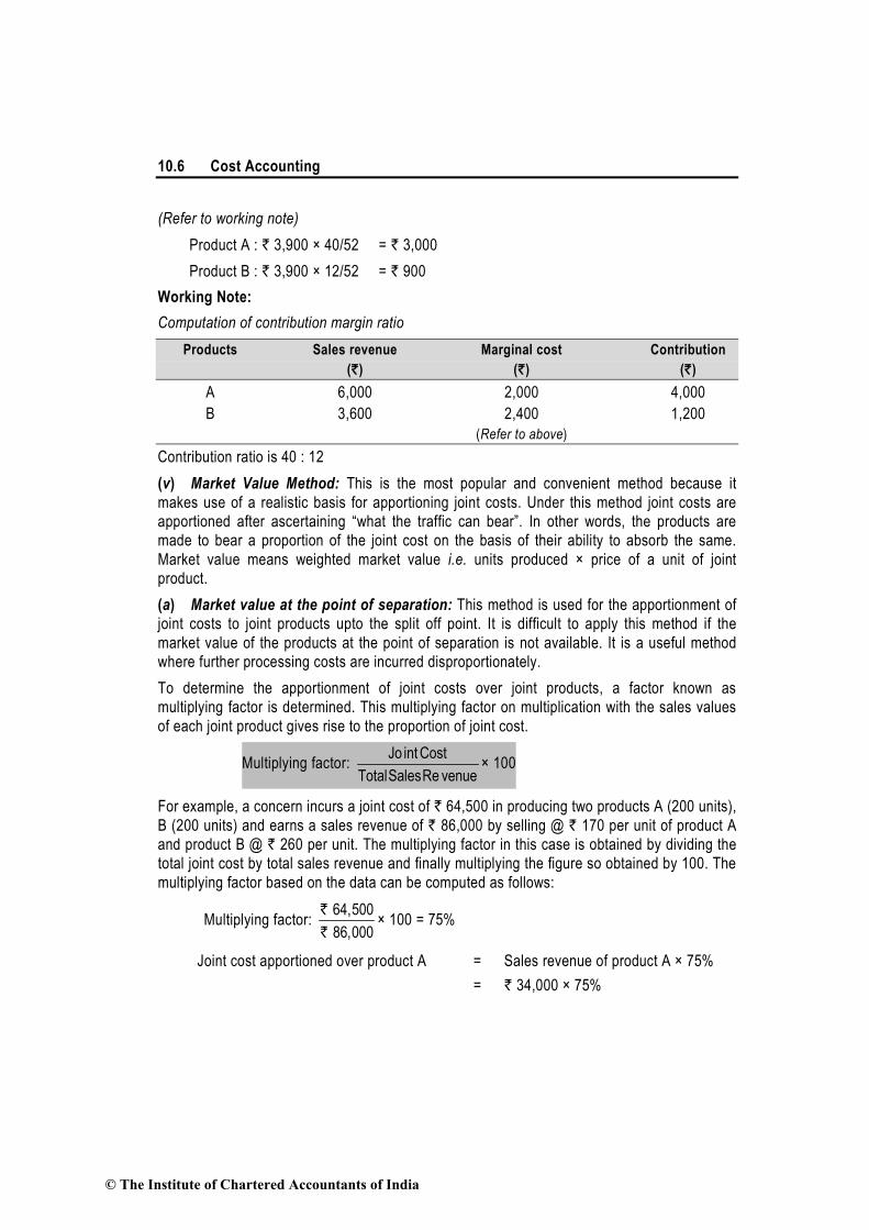
10.6 Cost Accounting
(Refer to working note)
Product A : ` 3,900 × 40/52 = ` 3,000
Product B : ` 3,900 × 12/52 = ` 900
Working Note:
Computation of contribution margin ratio
Products Sales revenue Marginal cost Contribution
(`) (`) (`)
A 6,000 2,000 4,000
B 3,600 2,400 1,200
(Refer to above)
Contribution ratio is 40 : 12
(v) Market Value Method: This is the most popular and convenient method because it
makes use of a realistic basis for apportioning joint costs. Under this method joint costs are
apportioned after ascertaining “what the traffic can bear”. In other words, the products are
made to bear a proportion of the joint cost on the basis of their ability to absorb the same.
Market value means weighted market value i.e. units produced × price of a unit of joint
product.
(a) Market value at the point of separation: This method is used for the apportionment of
joint costs to joint products upto the split off point. It is difficult to apply this method if the
market value of the products at the point of separation is not available. It is a useful method
where further processing costs are incurred disproportionately.
To determine the apportionment of joint costs over joint products, a factor known as
multiplying factor is determined. This multiplying factor on multiplication with the sales values
of each joint product gives rise to the proportion of joint cost.
Multiplying factor: Jo int Cost
TotalSalesRe venue× 100
For example, a concern incurs a joint cost of ` 64,500 in producing two products A (200 units),
B (200 units) and earns a sales revenue of ` 86,000 by selling @ ` 170 per unit of product A
and product B @ ` 260 per unit. The multiplying factor in this case is obtained by dividing the
total joint cost by total sales revenue and finally multiplying the figure so obtained by 100. The
multiplying factor based on the data can be computed as follows:
Multiplying factor: 64,500
86,000
`
` × 100 = 75%
Joint cost apportioned over product A = Sales revenue of product A × 75%
= ` 34,000 × 75%
© The Institute of Chartered Accountants of India

Joint Products & By-Products 10.7
= ` 25,500
Joint cost apportioned over product B = Sales revenue of product B × 75%
= ` 52,000 × 75%
= ` 39,000
Alternatively - This joint cost may be apportioned in the ratio of sales values of different joint
products.
(b) Market value after processing: Here the basis of apportionment of joint cost is the total
sales value of finished products and involves the same principle as discussed in (a) above.
Suppose that in the example given in Part (a) above, if sales prices of products A and B after
further processing are ` 200 and ` 300 respectively the joint cost apportioned over Products A
and B is as follows:
The pre-separation costs of ` 64,500 will be apportioned in the ratio of (2 : 3) as follows:
Market sales value after further processing
(`)
A : 200 units × ` 200 = 40,000
B : 200 units × ` 300 = 60,000
1,00,000
Joint cost apportioned :
A = ` 64,500 × `
`
40,000
1,00,000= ` 25,800
B = ` 64,500 × `
`
60,000
1,00,000 = ` 38,700
The use of this method is unfair where further processing costs after the point of separation
are disproportionate or when all the joint products are not subjected to further processing. The
net realisable value method which is discussed as below overcomes the shortcoming of this
method.
(c) Net realisable value method: From the sales value of the joint products (at finished
stage) the followings are deducted:
(i) estimated profit margins,
(ii) selling and distribution expenses, if any, and
(iii) post-split off costs.
The resultant figure so obtained is known as net realisable value of joint products. Joint costs
are apportioned in the ratio of net realisable value. Suppose that in the example given in part
© The Institute of Chartered Accountants of India

10.8 Cost Accounting
(a) above if further processing costs for products A and B are ` 4,000 and ` 32,000
respectively the Joint cost may be apportioned to products A and B as follows:
Products Sales Further Net realisable Joint cost
revenue (`) processing value apportionment
cost (`) (`) ratio
(a) (b) (c)=(a)–(b)
A 34,000 4,000 30,000 3/5
B 52,000 32,000 20,000 2/5
Joint cost apportioned over product A = ` 64,500 × 3/5 = ` 38,700
Joint cost apportioned over product B = ` 64,500 × 2/5 = ` 25,800
This method is extensively used in many industries.
Illustration 13 (Apportionment of joint cost under different methods)
Inorganic Chemicals purchases salt and processes it into more refined products such as
Caustic Soda, Chlorine and PVC. In the month of July, Inorganic Chemicals purchased Salt for
`40,000. Conversion of ` 60,000 were incurred upto the split off point, at which time two
sealable products were produced. Chlorine can be further processed into PVC.
The July production and sales information is as follows:
Production Sales quantity Selling price
(tonne) (tonne) (per tonne)
Caustic Soda 1,200 1,200 ` 50
Chlorine 800 — —
PVC 500 500 `200
All 800 tonnes of Chlorine were further processed, at an incremental cost of ` 20,000 to yield
500 tonnes of PVC. There was no beginning or ending inventories of Caustic Soda, Chlorine
or PVC in July.
There is active market for Chlorine. Inorganic Chemicals could have sold all its July production
of Chlorine at ` 75 per tonne.
Required :
(1) To calculate how joint cost of `1,00,000 would be apportioned between Caustic Soda and Chlorine under each of following methods :
(a) Sales value at split off,
(b) Physical measure (method), and
(c) Estimated net realisable value.
© The Institute of Chartered Accountants of India

Joint Products & By-Products 10.9
(2) Lifetime Swimming Pool Products offers to purchase 800 tonnes of Chlorine in August at `75 per tonne. This sale of Chlorine would mean that no PVC would be produced in August. How the acceptance of this offer for the month of August would affect operating income ?
Solution:
1. (a) Sales value at split off method
Products Sales in Selling price Sales Joint cost tonnes per tonne revenue apportioned*
(`) (`) (`)
(a) (b) (c)=(a) × (b)
Caustic Soda 1,200 50 60,000 50,000
Chlorine 800 75 60,000 50,000
1,20,000 1,00,000
* Apportioned joint cost = value sale Total
costjoint Total × Sale revenue of each product
Joint cost apportioned to Caustic Soda = 1,00,000
1,20,000
`
` × ` 60,000 = `50,000
Joint cost apportioned to Chlorine = `
`
1,00,000
1,20,000× `60,000 = `50,000
(b) Physical measure method
Products Sale in Joint cost (`)
(tonnes) apportioned **
Caustic Soda 1,200 60,000
Chlorine 800 40,000
2,000 1,00,000
**Apportioned joint cost =
Total jo int cos t
Total physical value × Physical units of each product
Joint cost apportioned to Caustic Soda = 1,00,000
2,000 tonnes
`
× 1,200 tonnes = `60,000
Joint cost apportioned to chlorine = 1,00,000
2,000 tonnes
`
× 800 tonnes = `40,000
© The Institute of Chartered Accountants of India

10.10 Cost Accounting
(c) Estimated net realisable value method
Products Sale Further Net realisable Apportioned***
revenue processing value Joint cost
(`) cost (`) (`) (`)
(a) (b) (c) = (a) – (b)
Caustic Soda 60,000 – 60,000 42,857
(1,200 tonnes × `50)
Chlorine 1,00,000 20,000 80,000 57,143
(500 tonnes of PVC × `200) ________ _______
1,40,000 1,00,000
**Apportioned joint cost = Total jo int cos t
Total net realisable value
× Net realisable value of each
product
Apportioned joint cost for Caustic Soda = 1,00,000
1,40,000
`
` × `60,000 = `42,857
Apportioned joint cost for Chlorine = 1,00,000
1,40,000
`
` × `80,000 = `57,143
2. Incremental revenue from further processing of Chlorine into PVC
(500 tonnes × `200 – 800 tonnes × `75) `40,000
Less : Incremental cost of further processing of Chlorine into PVC `20,000
Incremental operating income from further processing `20,000
The operating income of Inorganic Chemicals will be reduced by `20,000 in August if it sells
800 tonnes of Chlorine to Lifetime Swimming Pool Products, instead of further processing of
Chlorine into PVC for sale.
Illustration 5 (Preparation of income forecast statement and suggest production plan)
Sun-moon Ltd. produces 2,00,000 : 30,000; 25,000; 20,000 and 75,000 units of its five
products A, B, C, D and E respectively in a manufacturing process and sells them at ` 17,
` 13, ` 8, ` 10 and ` 14 per unit. Except product D remaining products can be further
processed and then can be sold at ` 25, ` 17, ` 12 and ` 20 per unit in case of A, B, C and E
respectively.
Raw material costs ` 35,90,000 and other manufacturing expenses cost ` 5,47,000 in the
manufacturing process which are absorbed on the products on the basis of their ‘Net
realisable value’. The further processing costs of A, B, C and E are ` 12,50,000; ` 1,50,000;
` 50,000 and ` 1,50,000 respectively. Fixed costs are ` 4,73,000.
You are required to prepare the following in respect of the coming year:
© The Institute of Chartered Accountants of India

Joint Products & By-Products 10.11
(a) Statement showing income forecast of the company assuming that none of its products
are to be further processed.
(b) Statement showing income forecast of the company assuming that products A, B, C and
E are to be processed further.
Can you suggest any other production plan whereby the company can maximise its
profits? If yes, then submit a statement showing income forecast arising out of adoption
of that plan.
Solution:
Working Note:
Statement showing apportionment of joint costs
on net realisable value basis
Products Sales value Post Net realisable Apportioned
separation value joint costs (1) (2) (1)–(2)=(3) (4) (`) (`) (`) (`)
A 50,00,000 12,50,000 37,50,000 26,25,000 (2,00,000 units × ` 25)
B 5,10,000 1,50,000 3,60,000 2,52,000 (30,000 units × ` 17)
C 3,00,000 50,000 2,50,000 1,75,000 (25,000 units × ` 12)
D 2,00,000 — 2,00,000 1,40,000 (20,000 units × ` 10)
E 15,00,000 1,50,000 13,50,000 9,45,000
(75,000 units × ` 20) _________ ________ 59,10,000 41,37,000
Total joint cost = Raw material costs + Manufacturing expenses
= ` 35,90,000 + ` 5,47,000 = ` 41,37,000
Apportioned joint cost = value realisablenet Total
costjoint Total× Net realisable value of each product
Apportioned joint cost for Product A = 41,37,000
59,10,000
`
` × ` 37,50,000 = ` 26,25,000
Similarly, the apportioned joint cost for products B, C, D and E are ` 2,52,000; ` 1,75,000; ` 1,40,000 and ` 9,45,000 respectively.
(a) Statement showing income forecast of the company assuming that none of its products are further processed
© The Institute of Chartered Accountants of India
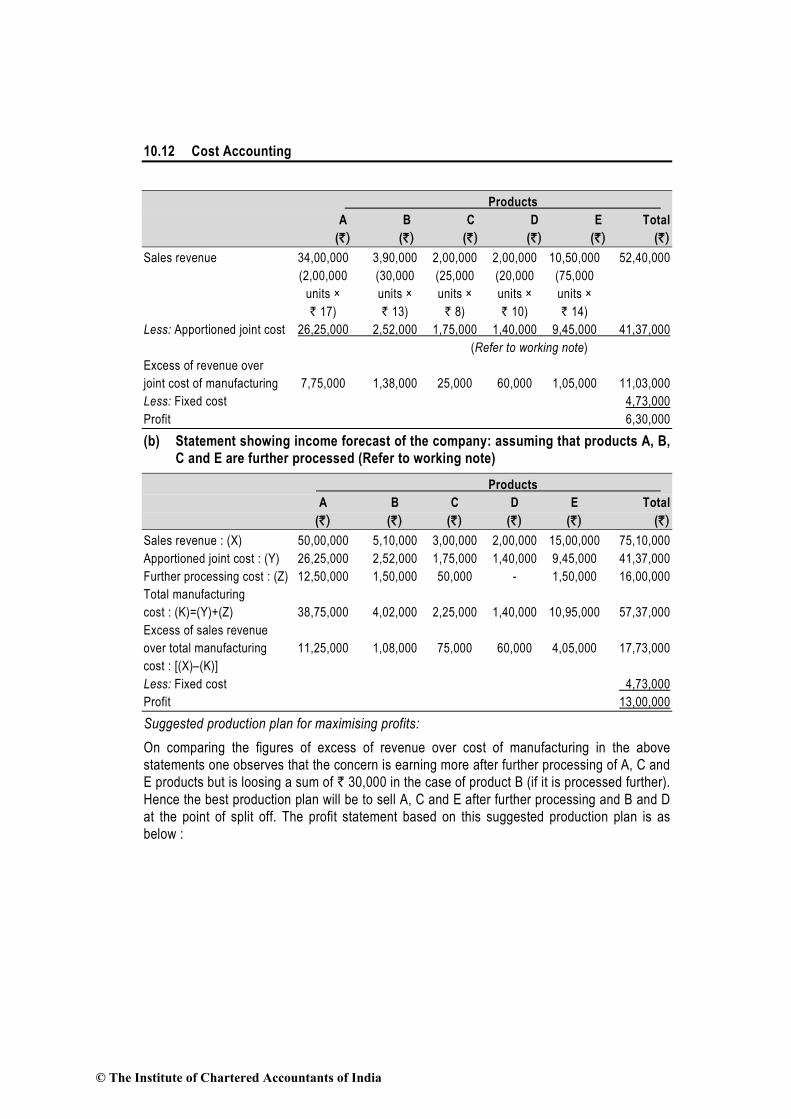
10.12 Cost Accounting
Products
A B C D E Total
(`) (`) (`) (`) (`) (`)
Sales revenue 34,00,000 3,90,000 2,00,000 2,00,000 10,50,000 52,40,000
(2,00,000 (30,000 (25,000 (20,000 (75,000
units × units × units × units × units ×
` 17) ` 13) ` 8) ` 10) ` 14)
Less: Apportioned joint cost 26,25,000 2,52,000 1,75,000 1,40,000 9,45,000 41,37,000
(Refer to working note)
Excess of revenue over
joint cost of manufacturing 7,75,000 1,38,000 25,000 60,000 1,05,000 11,03,000
Less: Fixed cost 4,73,000
Profit 6,30,000
(b) Statement showing income forecast of the company: assuming that products A, B,
C and E are further processed (Refer to working note)
Products
A B C D E Total
(`) (`) (`) (`) (`) (`)
Sales revenue : (X) 50,00,000 5,10,000 3,00,000 2,00,000 15,00,000 75,10,000
Apportioned joint cost : (Y) 26,25,000 2,52,000 1,75,000 1,40,000 9,45,000 41,37,000
Further processing cost : (Z) 12,50,000 1,50,000 50,000 - 1,50,000 16,00,000
Total manufacturing
cost : (K)=(Y)+(Z) 38,75,000 4,02,000 2,25,000 1,40,000 10,95,000 57,37,000
Excess of sales revenue
over total manufacturing 11,25,000 1,08,000 75,000 60,000 4,05,000 17,73,000
cost : [(X)–(K)]
Less: Fixed cost 4,73,000
Profit 13,00,000
Suggested production plan for maximising profits:
On comparing the figures of excess of revenue over cost of manufacturing in the above
statements one observes that the concern is earning more after further processing of A, C and
E products but is loosing a sum of ` 30,000 in the case of product B (if it is processed further).
Hence the best production plan will be to sell A, C and E after further processing and B and D
at the point of split off. The profit statement based on this suggested production plan is as
below :
© The Institute of Chartered Accountants of India

Joint Products & By-Products 10.13
Profit statement based on suggested production plan
Products
A B C D E Total
(`) (`) (`) (`) (`) (`)
1 2 3 4 5 6 7
Sales revenue : (X) 50,00,000 3,90,000 3,00,000 2,00,000 15,00,000 73,90,000
Appointed joint cost : (Y) 26,25,000 2,52,000 1,75,000 1,40,000 9,45,000 41,37,000
Further processing cost : (Z) 12,50,000 - 50,000 - 1,50,000 14,50,000
Total manufacturing
cost : (K)=(Y)+(Z) 38,75,000 2,52,000 2,25,000 1,40,000 10,95,000 55,87,000
Excess of sales revenue
over manufacturing cost 11,25,000 1,38,000 75,000 60,000 4,05,000 18,03,000
: [(X)–(K)]
Less: Fixed cost 4,73,000
Profit 13,30,000
Hence the profit of the company has increased by ` 30,000.
10.4 Methods of apportioning joint cost over by-products
The following methods may be adopted for the accounting of by-products and arriving at the
cost of production of the main product:
(a) Market value or value on realisation: The realisation on the disposal of the by-product
may be deducted from the total cost of production so as to arrive at the cost of the main
product. For example, the amount realised by the sale of molasses in a sugar factory goes to
reduce the cost of sugar produced in the factory.
When the by-product requires some additional processing and expenses are incurred in
making it saleable to the best advantage of the concern, the expenses so incurred should be
deducted from the total value realised from the sale of the by-product and only the net
realisations should be deducted from the total cost of production to arrive at the cost of
production of the main product. Separate accounts should be maintained for collecting
additional expenses incurred on :
(i) further processing of the by-product, and
(ii) selling, distribution and administration expenses attributable to the by-product.
(b) Standard cost in technical estimates: By-products may be valued at standard costs.
The standard may be determined by averaging costs recorded in the past and making
technical estimates of the number of units of original raw material going into the main product
and the number forming the by-product or by adopting some other consistent basis.
This method may be adopted where the by-product is not saleable in the condition in which it
© The Institute of Chartered Accountants of India

10.14 Cost Accounting
emerges or comparative prices of similar products are not available.
(c) Comparative price: Under this method, the value of the by-product is ascertained with
reference to the price of a similar or an alternative material.
Suppose in a large automobile plant a blast furnace not only produces the steel required for the car bodies but also produces gas which is utilised in the factory. This gas can be valued at the price which would have been paid to a gas company if the factory were to buy it from outside sources.
(d) Re-use basis: In some cases the by-product may be of such a nature that it can be reprocessed in the same process as part of the input of the process. In that case the value put on the by-product should be same as that of the materials introduced into the process. If, however, the by-product can be put into an earlier process only, the value should be the same as for the materials introduced into the process.
10.5 Treatment of By-Product Cost in Cost-Accounting
By-product cost can be dealt in cost accounting in the following ways:
(a) When they are of small total value: When the by-products are of small total value, the
amount realised from their sale may be dealt in any one the following two ways :
1. The sales value of the by-products may be credited to the Profit and Loss Account and
no credit be given in the Cost Accounts. The credit to the Profit and Loss Account here is
treated either as miscellaneous income or as additional sales revenue.
2. The sale proceeds of the by-product may be treated as deductions from the total costs.
The sale proceeds in fact should be deducted either from the production cost or from the
cost of sales.
(b) When the by-products are of considerable total value: Where by-products are of
considerable total value, they may be regarded as joint products rather than as by-products.
To determine exact cost of by-products the costs incurred upto the point of separation, should
be apportioned over by-products and joint products by using a logical basis. In this case, the
joint costs may be divided over joint products and by-products by using relative market values;
physical output method (at the point of split off) or ultimate selling prices (if sold).
(c) Where they require further processing: In this case, the net realisable value of the by-
product at the split-off point may be arrived at by subtracting the further processing cost from
the realisable value of by-products.
If total sales value of by-products at split-off point is small, it may be treated as per the
provisions discussed above under (a).
In the contrary case, the amount realised from the sale of by-products will be considerable and
thus it may be treated as discussed under (b).
© The Institute of Chartered Accountants of India

Joint Products & By-Products 10.15
10.6 Summary
Joint Products - Two or more products of equal importance, produced, simultaneously from
the same process, with each having a significant relative sale value are known as joint
products.
Co-Products - Two or more products which are contemporary but do not emerge necessarily
from the same material in the same process.
By-Products - Products recovered from material discarded in a main process, or from the
production of some major products.
Method of apportioning joint cost over joint products:
The commonly used methods for apportioning total process costs upto the point of separation
over the joint products are as follows:
(i) Physical unit method
(ii) Average unit cost method
(iii) Survey method
(iv) Contribution margin method
(v) Market value method:
(a) At the point of separation
(b) After further processing
(c) Net realisable value.
Methods of apportioning joint cost over by-products:
(a) Market value or value on realisation- The realisation on the disposal of the by-product
may be deducted from the total cost of production so as to arrive at the cost of the main
product.
(b) Standard cost in technical estimates- The standard may be determined by averaging
costs recorded in the past and making technical estimates of the number of units of original
raw material going into the main product and the number forming the by-product or by
adopting some other consistent basis.
This method may be adopted where the by-product is not saleable in the condition in which it
emerges or comparative prices of similar products are not available.
(c) Comparative price- Value of the by-product is ascertained with reference to the price of a
similar or an alternative material.
© The Institute of Chartered Accountants of India

10.16 Cost Accounting
(d) Re-use basis- The value put on the by-product should be same as that of the materials
introduced into the process.
Treatment of By-Product Cost in Cost-Accounting
(i) When they are of small total value:
1. The sales value of the by-products may be credited to the Profit and Loss Account
and no credit be given in the Cost Accounts. The credit to the Profit and Loss
Account here is treated either as miscellaneous income or as additional sales
revenue.
2. The sale proceeds of the by-product may be treated as deductions from the total
costs. The sale proceeds in fact should be deducted either from the production cost
or from the cost of sales.
(ii) When the by-products are of considerable total value - The joint costs may be divided
over joint products and by-products by using relative market values; physical output
method (at the point of split off) or ultimate selling prices (if sold).
(iii) Where they require further processing -The net realisable value of the by-product at the
split-off point may be arrived at by subtracting the further processing cost from the
realisable value of by-products.
If total sales value of by-products at split-off point is small, it may be treated as per the
provisions discussed above under (i).
In the contrary case, the amount realised from the sale of by-products will be considerable and
thus it may be treated as discussed under (ii).
© The Institute of Chartered Accountants of India

11 Standard Costing
Learning Objectives
After studying this chapter you should be able to;
• Understand the meaning of standard cost and variances.
• Understand the concept of capacity with reference to a product cost sheet.
• Understand the difference between controllable and uncontrollable variances.
• Compute variances related to material, labour, overhead and sales.
• Understand the reporting pattern which may be adopted for control and decision making
purposes.
• Understand the meaning of disposition of variances.
• Understand the advantages and disadvantages of standard costing and variance analysis.
11.1 Introduction
Standard Costing is a method of costing which is used as a control tool by the management.
Controlling is a principal function of management alongwith planning, directing and staffing. Every
organisation sets a goal and to achieve it management of the organisation make plans, get these
plans executed and monitor the work for any deviation from the plan. Please note the word
deviation. Deviation means the amount by which a single measurement differs from a fixed
value such as the mean or standard (here it is used in the context of cost accounting).
Deviation is measured by comparing actual figure with the standard figure.
11.1.1 What is a standard or Standard Cost?
Standard cost is defined in the CIMA Official Terminology as “'the planned unit cost of the
product, component or service produced in a period. The standard cost may be determined on
a number of bases. The main use of standard costs is in performance measurement, control,
stock valuation and in the establishment of selling prices.” From the above definition Standard
costs can be said as
© The Institute of Chartered Accountants of India
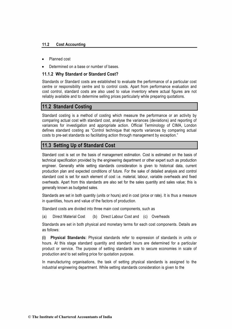
11.2 Cost Accounting
• Planned cost
• Determined on a base or number of bases.
11.1.2 Why Standard or Standard Cost?
Standards or Standard costs are established to evaluate the performance of a particular cost centre or responsibility centre and to control costs. Apart from performance evaluation and cost control, standard costs are also used to value inventory where actual figures are not reliably available and to determine selling prices particularly while preparing quotations.
11.2 Standard Costing
Standard costing is a method of costing which measure the performance or an activity by comparing actual cost with standard cost, analyse the variances (deviations) and reporting of variances for investigation and appropriate action. Official Terminology of CIMA, London defines standard costing as “Control technique that reports variances by comparing actual costs to pre-set standards so facilitating action through management by exception.”
11.3 Setting Up of Standard Cost
Standard cost is set on the basis of management estimation. Cost is estimated on the basis of
technical specification provided by the engineering department or other expert such as production
engineer. Generally while setting standards consideration is given to historical data, current
production plan and expected conditions of future. For the sake of detailed analysis and control
standard cost is set for each element of cost i.e. material, labour, variable overheads and fixed
overheads. Apart from this standards are also set for the sales quantity and sales value; this is
generally known as budgeted sales.
Standards are set in both quantity (units or hours) and in cost (price or rate). It is thus a measure
in quantities, hours and value of the factors of production.
Standard costs are divided into three main cost components, such as
(a) Direct Material Cost (b) Direct Labour Cost and (c) Overheads
Standards are set in both physical and monetary terms for each cost components. Details are
as follows:
(i) Physical Standards: Physical standards refer to expression of standards in units or
hours. At this stage standard quantity and standard hours are determined for a particular
product or service. The purpose of setting standards are to secure economies in scale of
production and to set selling price for quotation purpose.
In manufacturing organisations, the task of setting physical standards is assigned to the
industrial engineering department. While setting standards consideration is given to the
© The Institute of Chartered Accountants of India

Standard Costing 11.3
Company’s operating plan i.e. budgets
Final output to be produced
Material specification, in both quantity and quality provided by the engineering
department.
Proportion of material to be used in case of multiple inputs.
Method of production i.e. fully automated, semi-automated or manual.
Skill set of workers and availability of workers.
Working conditions and internal factors.
External factors (such as Labour Law, Factories Act, Govt. policy etc.).
Material quantity standards: The following procedure is usually followed for setting material
quantity standards.
(a) Standardisation of products: At this phase products to be produced is decided based on
production plan and customer’s order. Generally following questions are answered at this
stage: (i) What to be produced? (ii) Which type to be produced and (iii) How much to be
produced?
(b) Product study: Product to be produced is analysed and studied for developments and
production. Product study is carried out by the engineering department or product
consultants. At this phase answers to the following questions are satisfied: (i) How can it
be produced? (ii) What are the pre-requisites? (iii) Which type of materials to be used?
(iv) How products can be accepted in the market? Etc.
(c) Preparation of specification list: After the product study a list of material is prepared. It
specifies types (quality) and quantity of materials to be used, substitute of the materials,
quantity and proportion of materials to be used, process to be followed, pre-requisites
and condition required etc. While preparing specification list consideration to expected
amount of wastage is given. It must be customised to adopt changes in the product.
(d) Test runs: Sample or test runs under specified conditions are carried out and sample
products are tested for the desired quality and quantity. Any deviation from the
specification is noted down and specification list is updated.
Labour time standards: The following are the steps involved in setting labour quantity
standards:
(a) Standardisation of product and product study is carried out as explained above.
(b) Labour specification: Types of labour and labour time is specified. Labour time
specification is based on past records and it takes into account normal wastage of time.
© The Institute of Chartered Accountants of India

11.4 Cost Accounting
(c) Standardisation of methods: Selection of proper machines to use proper sequence and
method of operations.
(d) Manufacturing layout: A plan of operation for each product listing the operations to be
performed is prepared.
(e) Time and motion study: It is conducted for selecting the best way of completing the job or
motions to be performed by workers and the standard time which an average worker will
take for each job. This also takes into account the learning efficiency and learning effect.
(f) Training and trial: Workers are trained to do the work and time spent at the time of trial run is
noted down.
Overheads time/ quantity standards: Variable overhead time/ quantity is estimated based on
specification made by the engineering departments. Variable overheads may either be based on
direct material quantity or labour hour. Generally it is based on labour time worked.
Fixed overhead time is based on budgeted production volume.
Problems faced while setting physical standards: The problems involved while setting
physical standards will vary from industry to industry and may be illustrated as under:
(a) A situation may arise where the company is introducing the manufacture of a new line of
product. In such case, it may be necessary to employ workers who have no experience
in the job. This creates a problem of setting standard time because it is necessary to
make adjustment for the inexperience of workers.
(b) Changes in technology may necessitate installation of sophisticated machines. When
such machines are installed, the precise estimation of output and standard of efficiency
achievable will pose a problem until after a long time when the working conditions are
settled. Thus, setting standards for these machines and estimating the standard costs
will need considerable amount of work.
(c) Often manufacturers prefer to product diversification to improve profitability. One of the
most important problems that arise with the proposed change in product is re-setting of
production facilities. For example, when an old copper part is to be changed into one
made of bronze to suit the new product, special care has to be taken to order new tools
which in turn, pose the problem of setting up of standard time in respect of the new tools.
(d) Standards of material specifications are established and if the materials are not available
as per specifications, the standards may not be achievable.
(e) Very often the cost accountant is confronted with the problem of choosing the type of
standards to be adopted. For example, the industrial engineer has furnished the
standard time for all direct labour operations as under:
© The Institute of Chartered Accountants of India

Standard Costing 11.5
1. Standard time attainable by the best operations is 2 hours per unit of product
including allowances for personal fatigue and delay.
2. Attainable good performance for the average trained operator is 2.10 hours per unit
of product.
3. Average past performance is 2.60 hours per unit.
The problem is, should direct labour standard hour be based on maximum efficiency or
attainable good performance or average past performance? If costs are to represent maximum
efficiency, the unit cost used in selling price will relatively be low but a high debit variance may
arise if the standard efficiency is not achieved.
If, however, the standard cost is based on attainable good performance, the variances may
tend to be nil. If efficiency is to be gauged, maximum efficiency standard will reflect the off
standard performance, thereby enabling the departmental head to exercise control.
Similar problems as those mentioned above, may also arise in setting of waste standards. For
example, the question may arise as to whether only absolutely unavoidable wastage should be
provided or the past average level of wastage may be provided. This will again have different
impact on the standard cost of production.
(ii) Price or Rate Standards: Broadly, the price or rate standards can be set on either of
the following bases:
(a) Actual average or mean price expected to prevail during the coming period, say one
year; or
(b) Normal prices expected to prevail during a cycle of seasons which may be of a number of
years.
Material price standards: Material prices are not altogether within the control of the
manufacturer; but the purchasing department, on being apprised of production quantities
required, should be able, from its knowledge of current market conditions and trends, to state
with reasonable accuracy price for the constituent items. The standards for prices of materials
should be based on the following factors, if price fluctuations are small and are not serious.
(a) Stock of materials on hand and the prices at which they are held;
(b) The prices at which orders for future deliveries of materials (agreement entered into) have
already been placed,
(c) Minimum support price fixed by the appropriate authority and
(d) Anticipated fluctuation in price levels
© The Institute of Chartered Accountants of India

11.6 Cost Accounting
In case there are unsystematic fluctuations in the market price, it may be difficult to determine
standard costs of materials; fluctuations in the market price may be of different sorts; prices
may be different from month to month, from one season to another or from one year to
another. There may be a secular trend which, on the whole, is pushing price upwards or
downwards. The nature of difficulties encountered in fixing standard costs of materials will
naturally be different in each case. In addition the purchasing policy of the company and the
objective to be achieved (from cost accounting) will make a difference.
The difficulty in determining the standard cost of material in such a situation can be resolved
as follows:
(a) In case prices fluctuate from month to month, the average of prices of a year corrected
for the known secular changes and any other expected change can very well serve as
the standard price for the next year.
(b) If the fluctuations are seasonal, but the whole year’s requirements are purchased at one
time, the weighted average of the likely prices to be paid should be treated as the
standard price. But, if buying is also spread over the whole year, the weighted average
of the prices for the whole year should be the standard price.
(c) If prices fluctuate from one year to another, a careful estimate of the price likely to prevail
next year, based on a statistical study, should be adopted as the standard price.
Wage rate standard: The type of labour required for performing a specific job would be the
most important factor for deciding the rate of wage to be paid to workers. Standard wage rate
for skilled and unskilled workers are set based on the following basis:
Time taken by the workers to complete a unit of production.
Time or piece rate prevailing in the industry. It can be known from the peers.
Wage agreement entered into between the management and workers’ union.
Law prevailing in the area of operation, law like Payment of minimum wages Act,
Payment of bonus Act etc.
Overhead expense standards: In computing the overhead expense standards, consideration
should be given to the level of output and the expenses budgeted. A budget showing the level
of output to be considered for arriving at overhead expense standards may be based on the
practical manufacturing capacity or the average sales capacity or the budgeted capacity to be
utilised in the coming year. After having chosen one of the bases for computing output level,
the expenses can be budgeted under different heads for the level of output chosen. These
expenses are classified under fixed and variable categories. Thus, the overhead expenses
standards are set by computing the optimum level of output for the production departments
and thereafter drafting a budget for fixed and variable expenses which will be incurred at this
level. If production is seasonal or it fluctuates during the year, a flexible budget may be
prepared to facilitate comparison between the target set and the actual expenditure for the
period.
© The Institute of Chartered Accountants of India

Standard Costing 11.7
11.4 Types of Standards
The accuracy and relevance of an established standard cost depends upon the reliability of
the standards being set up. In order to set standards we must know the degree of accuracy
proximity of the standards with the actual result. Below are the few standards have been
discussed below:
(i) Ideal Standards: These represent the level of performance attainable when prices for
material and labour are most favourable, when the highest output is achieved with the best
equipment and layout and when the maximum efficiency in utilisation of resources results in
maximum output with minimum cost.
These types of standards are criticised on three grounds:
(a) Since such standards would be unattainable, no one would take these seriously.
(b) The variances disclosed would be variances from the ideal standards. These would not,
therefore, indicate the extent to which they could have been reasonably and practically
avoided.
(c) There would be no logical method of disposing of these variances.
(ii) Normal Standards: These are standards that may be achieved under normal operating
conditions. The normal activity has been defined as “the number of standard hours which will produce
at normal efficiency sufficient good to meet the average sales demand over a term of years”.
These standards are, however, difficult to set because they require a degree of forecasting.
The variances thrown out under this system are deviations from normal efficiency, normal
sales volume, or normal production volume.
If the actual performance is found to be abnormal, large variances may result and necessitate
revision of standards.
(iii) Basic or Bogey Standards: These standards are used only when they are likely to
remain constant or unaltered over a long period. According to this standard, a base year is
chosen for comparison purposes in the same way as statisticians use price indices. Since
basic standards do not represent what should be attained in the present period, current
standards should also be prepared if basic standards are used. Basic standards are, however,
well suited to businesses having a small range of products and long production runs. Basic
standards are set, on a long-term basis and are seldom revised. When basic standards are in
use, variances are not calculated. Instead, the actual cost is expressed as a percentage of
basic cost. The current cost is also similarly expressed and the two percentages are
compared to find out how much the actual cost has deviated from the current standard. The
percentages are next compared with those of the previous periods to establish the trend of
© The Institute of Chartered Accountants of India

11.8 Cost Accounting
actual and current standard from basic cost.
(iv) Current Standards: These standards reflect the management’s anticipation of what
actual costs will be for the current period. These are the costs which the business will incur if
the anticipated prices are paid for the goods and services and the usage corresponds to that
believed to be necessary to produce the planned output.
The variances arising from expected standards represent the degree of efficiency in usage of
the factors of production, variation in prices paid for materials and services and difference in
the volume of production.
11.5 Need for Standard Costs
Standard costing system is widely accepted as it serves the different needs of an organisation. The
standard costing is preferred for the following reasons:
(a) Prediction of future cost for decision making: Standard costs are set after taking into
account all the future possibilities and can be termed as future cost. Standard cost is
used for calculating profitability from a project/ order/ activity proposed to be undertaken.
Hence, standard cost is very useful for decision making purpose.
(b) Provide target to be achieved: Standard costs are the target cost which should be no
be crossed. It keeps challenging target before the responsibility centres. Management of
responsibility centres monitor the performance continuously against the set standards
and deviations are immediately corrected.
(c) Used in budgeting and performance evaluation: Standard costs are used to set
budgets and based on these budgets managerial performance is evaluated. This is of two
benefits, one managers of a responsibility centre will not compromise with the quality to
fulfill the budgeted quantity and second, variances can be traced with the responsible
department or person.
(d) Interim profit measurement and inventory valuation: Actual profit is known only after
the closure of the account. Few organisations used to prepare profitability statement for
some interim periods as per the requirement of the management. To arrive at the
profitability figure standard costs are deducted from the revenue.
11.6 The Process of Standard Costing
The process of standard cost is as below:
(i) Setting of Standards: The first step is to set standards which are to be achieved, the
process of standard setting is explained above.
(ii) Ascertainment of actual costs: Actual cost for each component of cost is ascertained.
© The Institute of Chartered Accountants of India

Standard Costing 11.9
Actual costs are ascertained from books of account, material invoices, wage sheet, charge slip
etc.
(iii) Comparison of actual cost and standard cost: Actual costs are compared with the
standards costs and variances are determined.
(iv) Investigation of variances: Variances arises are investigated for further action. Based
on this performance is evaluated and appropriate actions are taken.
(v) Disposition of variances: Variances arise are disposed off by transferring it the relevant
accounts (costing profit and loss account) as per the accounting method (plan) adopted.
11.7 Types of Variances
11.7.1 Controllable and un-controllable variances: The purpose of the standard
costing reports is to investigate the reasons for significant variances so as to identify the
problems and take corrective action.
Variances are broadly of two types, namely, controllable and uncontrollable. Controllable
variances are those which can be controlled by the departmental heads whereas uncontrollable
variances are those which are beyond their control. Responsibility centres are answerable for all
adverse variances which are controllable and are appreciated for favourable variances.
Controllability is a subjective matter and varies from situation to situation. If the uncontrollable
variances are of significant nature and are persistent, the standard may need revision.
11.7.2 Favourable and Adverse variance: Favourable variances are those which are
profitable for the company and adverse variances are those which causes loss to the
company. While computing cost variances favourable variance means actual cost is less than
standard cost. On the other hand adverse variance means actual cost is exceeding standard
cost. The situation will be reversed for sales variance. Favourable variances means actual is
more than budgeted and on contrary adverse variance is where actual is less than budgeted.
These are credited and debited in the costing profit and loss account respectively. Favourable
variance in short denoted by capital ‘F’ and adverse variances by capital ‘A’.
Students may note that signs of favourable and adverse variance may or may not match exactly with mathematical signs i.e. (+) or (-).
11.8 Classification of Variances
Variances are broadly classified into two parts namely Revenue variance and Cost variance.
At Revenue side variances is calculated by comparing actual sales from budgeted (standard)
sales. On the other hand Cost side reflects variances in cost components. Cost variance
classification is shown below with the help of a structured diagram.
© The Institute of Chartered Accountants of India

11.10 Cost Accounting
Fig 8.1: Classification of Variances
11.8.1 Computation of variances: As discussed earlier variances are classified into two
parts. Here we will start from cost side and discuss all cost components one by one with the
help of appropriate example and illustrations.
(a) Material Cost Variance: Material cost variance is the difference between standard cost
and actual cost. Mathematically it is written as.
Material Cost variance = (Standard quantity x Standard Price) – (Actual quantity x
Actual price)
Or
MCV = (SQ × SP) – (AQ × AP)
Total Cost
Material Cost Variance
Labour Cost Variance
Overhead Cost Variance
Material Price
Variance
Material Usage
Variance
Labour Rate
Variance
Labour Efficiency Variance
Material Mix
Variance
Material Yield
Variance
Labour Mix
Variance
Idle Time
Variance
Labour Yield
Variance
Variable Overhead Cost Variance
Fixed Overhead Cost Variance
Expenditure or Budget Variance
Efficiency Variance
Expenditure or Budget Variance
Volume Variance
Efficiency Variance
Capacity Variance
Calendar Variance
© The Institute of Chartered Accountants of India

Standard Costing 11.11
Reasons: Material cost variance arises mainly because of either difference in material price
from the standard price or difference in material consumption from standard consumption or
because of both reasons. Analysis of material cost variance is done dividing it into two parts
namely Material Price variance and Material Usage variance.
(i) Material Price variance: It measures variance arises in the material cost due to
difference in actual material purchase price from standard material price. Mathematically it is
written as:
Material Price Variance = Actual quantity* × (Standard price – Actual price)
Or
MPV = AQ × (SP – AP)
*Here actual quantity means actual quantity of material purchased. If in the question material
purchase is not given, it is taken as equal to material consumed.
Material price variance can also be calculated taking material used as actual quantity instead of
material purchased. This method is also correct but does not serve the purpose of variance
computation. Material price variance may arise from variety of reasons out of which some may be
controllable and some may be beyond the control of the purchase department. If price variance arises
due to inefficiency of purchase department or any other reason within the control of the company,
then it is very important to report variance as early as possible and this can be done by taking
purchase quantity as actual quantity for price variance computation.
Responsibility: Generally, purchase department purchases materials from the market.
Purchase department is expected to perform its function very prudently so that company never
suffers loss due to its inefficiency. Purchase department is held responsible for adverse price
variance arises due to the factors controllable by the department.
(ii) Material Usage Variance: It measures variance in material cost due to usage/
consumption of materials. It is computed as below:
Material Usage variance = Standard price (Standard quantity – Actual quantity*)
Or
MUV = SP × (SQ –AQ)
*Here actual quantity means actual quantity of material used.
Responsibility: Material usage is the responsibility of production department and it is held
responsible for adverse usage variance.
Reasons of material usage variance: Actual material consumption may differ from the standard
quantity due to either difference in proportion used from standard proportion or due to
© The Institute of Chartered Accountants of India

11.12 Cost Accounting
difference in actual yield from standard yield. Material usage variance is divided into two parts
(iia) Material usage mix variance and (iib) Material yield variance.
(iia) Material Mix Variance: Variance in material consumption may arise due to difference in
proportion used actually from the standard mix/ proportion. It arises only when two more
inputs are used to produce a product. Mathematically,
Material Mix Variance = (Revised standard quantity – Actual quantity) × Standard price
Or
MMV = (RSQ – AQ) × SP
Where,
Revised standard quantity =
Standard quantity of one material
Total of actual quantities of all materialsTotal of standard quantitiets of all materials
×
(iib) Material Yield Variance (or Material Sub-usage Variance): Variance in material
consumption which arise due to yield or productivity of the inputs. It may arise due to use
of sub standard quality of materials, inefficiency of workers or due to wrong processing.
Material Revised usage variance = (Standard quantity – Revised standard quantity) ×
Standard price
MRUV = (SQ – RSQ) × SP
Or
Material Yield Variance = (Actual yield – Standard yield) × Standard output price
MYV = (AY – SY) × SOP
Note: Material revised usage variance is also known as material sub – usage variance.
In each case there will be only one variance either material yield or material revised usage
variance.
Verification of the formulae:
Material Cost Variance = Material Usage Variance + Material Price Variance*
Or, Material Cost Variance = (Material Mix Variance + Material Revised usage Variance) +
Material price variance
*If material purchase quantity and material consumed quantity is same
© The Institute of Chartered Accountants of India

Standard Costing 11.13
Meaning of the terms used in the formulae:
Term Meaning
Standard Quantity (SQ) Quantity of inputs to be used to produce actual output.
Actual Quantity (AQ) Quantity of inputs actually used to produce actual output.
Revised Standard Quantity (RSQ)
If Actual total quantity of inputs were used in standard proportion.
Actual Yield (AY) Actual Output
Standard Yield (SY) Actual output if inputs used in standard ratio
Standard Output Price (SOP)
Standard material cost for actual output
Illustration 1 (Calculation of material cost variance)
The standard and actual figures of product ‘Z’ are as under:
Standard Actual
Material quantity 50 units 45 units
Material price per unit ` 1.00 ` 0.80
Calculate material cost variance.
Solution:
The variances may be calculated as under:
(a) Standard cost = Std. qty × Std. price = 50 units × ` 1.00 = `50
(b) Actual cost = Actual qty. × Actual price = 45 units × ` 0.80 = ` 36
Variances:
(i) Price variance = Actual qty (Std. price – Actual price)
= 45 units (` 1.00 – ` 0.80) = ` 9 (F)
(ii) Usage variance = Std. price (Std. qty – Actual qty.)
= ` 1 (50 units – 45 units) = ` 5 (F)
(iii) Material cost variance = Standard cost – Actual cost
(Total variance) = ` 50 – ` 36 = ` 14 (F)
Illustration 2 (Calculation of material usage, price and total cost variance)
NXE Manufacturing Concern furnishes the following information:
Standard: Material for 70 kg finished products 100 kg.
Price of material ` 1 per kg.
Actual: Output 2,10,000 kg.
© The Institute of Chartered Accountants of India

11.14 Cost Accounting
Material used 2,80,000 kg.
Cost of Materials ` 2,52,000
Calculate: (a) Material usage variance, (b) Material price variance, (c) Material cost variance.
Solution:
Standard Quantity of input for actual output (SQ) = 2, 10,000 kg × kg70
kg100= 3, 00,000 kg.
Actual Price (AP) = (`2, 52,000 ÷ 2, 80,000 kg) = ` 0.90 per kg.
(a) Material Usage Variance = (SQ – AQ) × SP
= (3,00,000 – 2,80,000) × 1
= ` 20,000 (F)
(b) Material Price Variance = (SP – AP) × AQ
= (1 – 0.90) × 2,80,000
= ` 28, 000 (F)
(c) Material Cost Variance = (SQ × SP) – (AQ × AP)
= (3, 00,000 × 1) – (2, 80,000 × 0.90)
= ` 48, 000 (F)
Check MCV = MPV + MUV
` 48, 000 (F) = ` 28, 000 (F) + `20, 000 (F)
Illustration 3 (Calculation of Material cost, price and usage variance)
For making 10 kg. of CEMCO, the standard material requirements is:
Material Quantity Rate per kg. (`)
A 8 6.00
B 4 4.00
During April, 1,000 kg of CEMCO were produced. The actual consumption of materials is as under:
Material Quantity (Kg.) Rate per kg. (`)
A 750 7.00
B 500 5.00
Calculate (A) Material Cost Variance; (b) Material Price Variance; (c) Material usage Variance.
© The Institute of Chartered Accountants of India

Standard Costing 11.15
Solution:
Basic Calculations
Standard for 1,000 kg. Actual for 1,000 kg.
Qty. Rate Amount Qty. Rate Amount
Kg. (`) (`) Kg. (`) (`)
A 800* 6 4,800 750 7 5,250
B 400* 4 1,600 500 5 2,500
Total 1,200 6,400 1,250 7,750
(* A- 8÷10 ×1000 = 800 B- 4÷10 × 1000 = 400)
Calculation of Variances:
(a) Material Cost Variance = Std. cost for actual output – Actual cost
MCV = 6,400 – 7,750
= `1, 350 (A)
(b) Material Price Variance = (SP – AP) × AQ
A = (6 – 7) × 750 = ` 750 (A)
B = (4 – 5) × 500 = ` 500 (A)
MPV = `1,250 (A)
(c) Material Usages Variance = (SQ – AQ) × SP
A = (800 – 750) × 6 = ` 300 (F)
B = (400 – 500) × 4 = ` 400 (A)
MUV = ` 100 (A)
Check
MCV = MPV + MUV
1,350 (A) = 1,250 (A) + 100 (A)
Illustration 4 (Calculation of material mix and material yield variance)
The standard cost of a chemical mixture is as follows:
40% material A at ` 20 per kg.
60% material B at ` 30 per kg.
A standard loss of 10% of input is expected in production. The cost records for a period
showed the following usage :
90 kg material A at a cost of ` 18 per kg.
110 kg material B at a cost of ` 34 per kg.
© The Institute of Chartered Accountants of India

11.16 Cost Accounting
The quantity produced was 182 kg. of good product.
Calculate all material variances.
Solution:
Basic Calculation
Material Standard for 180 kg. output Actual for 182 kg. output
Qty.
Kg.
Rate
(`)
Amount
(`)
Qty
Kg.
Rate
(`)
Amount
(`)
A 80 20 1,600 90 18 1,620
B 120 30 3,600 110 34 3,740
Total 200 5,200 200 5,360
Less: Loss 20 − − 18 − −
180 5,200 182 5,360
Std. cost of actual output = `5, 200 × 180
182 = ` 5, 257.78
Calculation of Variances
1. Material Cost Variance = (Std. cost of actual output – Actual cost)
= (5,227.78 – 5,360) = ` 102.22 (A)
2. Material Price Variance = (SP – AP) × AQ
Material A = (20 – 18) × 90 = ` 180.00 (F)
Material B = (30 – 34)) × 110 = ` 440.00 (A)
MPV = ` 260.00 (A)
3. Material Usage Variance = (Std. Quantity for actual output – Actual Quantity) × Std. Price
Material A =
−× 90
180
18280 × 20 = ` 182.22 (A)
Material B =
−× 110
180
182120 × 30 = `340.00 (F)
MUV = `157.78 (F)
Check
MCV `102.22 (A)
MPV `260 (A) MUV `157.78 (F)
© The Institute of Chartered Accountants of India

Standard Costing 11.17
Illustration 5 (calculation of material mix variance and material yield variance)
The standard mix to produce one unit of product is as follows:
Material X 60 units @ ` 15 per unit = 900
Material Y 80 units @ ` 20 per unit = 1,600
Material Z 100 units @ ` 25 per unit = 2,500
240 units 5,000
During the month of April, 10 units were actually produced and consumption was as follows:
Material X 640 units @ ` 17.50 per unit = 11,200
Material Y 950 units @ ` 18.00 per unit = 17,100
Material Z 870 units @ ` 27.50 per unit = 23,925
2460 units 52,225
Calculate all material variances.
Solution:
Material
Standard for 10 units Actual for 10 units
Qty.
units
Rate
(`)
Amount
(`)
Qty.
units
Rate
(`)
Amount
(`)
X 600 15 9,000 640 17.50 11,200
Y 800 20 16,000 950 18.00 17,100
Z 1,000 25 25,000 870 27.50 23,925
Total 2,400 50,000 2460 52,225
1. Material Cost Variance = Standard cost – Actual cost
= ` 50,000 – ` 52,225
MCV = ` 2,225 (A)
2. Material Price Variance = (Std. Price – Actual Price) × Actual Qty.
Material X = (15 – 17.50) × 640 = ` 1,600 (A)
Material Y = (20 – 18) × 950 = ` 1,900 (F)
Material Z = (25 – 27.50) × 870 = ` 2,175 (A)
MPV = ` 1,875 (A)
3. Material Usage Variance = (Std. Qty. – Actual Qty.) × Std. Price
Material X = (600 – 640) × 15 = ` 600 (A)
Material Y = (800 – 950) × 20 = ` 3,000 (A)
Material Z = (1,000 – 870) × 25 = ` 3,250 (F)
MUV = ` 350 (A)
© The Institute of Chartered Accountants of India

11.18 Cost Accounting
Check MCV = MPV + MUV
`2,225 (A) = `1,875 (A) + `350 (A)
4. Material Mix Variance = (Revised Std. Qty. – Actual Qty.) × Std. Price
Material X = (615* – 640) × 15 = ` 375 (A)
Material Y = (820* – 950) × 20 = `2,600 (A)
Material Z = (1,025 – 870) × 25 = `3,875 (F)
MMV = ` 900 (F)
*Revised Standard Quantity (RSQ) is calculated as follows:
Material X = 2400
2460 × 600 = 615 units
Material Y = 2400
2460× 800 = 820 units
Material Z = 2400
2460 × 1,000 = 1,025 units
5. Material Yield Variance
For yield variance, certain basic calculations have to be made as follows :
Standard Yield Variance = output ofunit per usage Standard
materials of usage Actual=
2460
240= 10.25 units
SOP (Std. material cost per unit of output) = `50,000 ÷ 10 units = `5,000
Material Yield Variance = (AY – SY) × SOP
MYV = (10 – 10.25) × 5,000 = `1,250 (A)
Material Revised Usage (or Sub-usage) Variance (MRUV)
= (Standard Quantity – Revised Standard Quantity) × Standard Price
Material X = (600 – 615) × 15 = ` 225 (A)
Material Y = (800 – 820) × 20 = ` 400 (A)
Material Z = (1,000 – 1,025) × 25 = ` 625 (A)
MRUV = `1,250 (A)
Note : Either MMV or MRUV is calculated. These two are always equal.
Check
MUV = MMV + MYV (Or MRUV)
`350 (A) = `900 (F) + `1,250 (A)
or
MCV = MPV + MMV + MYV (Or MRUV)
`2,225 (A) = `1,875 (A) + `900 (F) + `1,250 (A)
© The Institute of Chartered Accountants of India

Standard Costing 11.19
(b) Labour Cost Variance: Labour cost variance is the difference between actual labour
cost and standard cost . Mathematically
Labour Cost Variance = (Std. hours for actual output × Std. rate per hour) – (Actual
hours × Actual rate per hour)
Or
LCV = (SH x SR) – (AH x AR)
Reason: Difference in labour cost arises either due to difference in the actual labour rate from
the standard rate or difference in numbers of hours worked from standard hours. Labour cost
variance can be divided into two parts namely (i) Labour Rate Variance and (ii) Labour
Efficiency Variance.
(i) Labour Rate Variance: Labour rate variance arises due to difference in actual rate paid
from standard rate. It is very similar to material price variance. It is calculated as below:
Labour Rate Variance = Actual time* (Std. rate – Actual rate)
LRV = AH x (SR – AR)
*Here actual time means time for which wage has been paid/ credited.
Responsibility: Generally labour rates are influenced by the external factors which are beyond
the control of the organisation. However personnel manager is responsible for labour rate
negotiation.
(ii) Labour Efficiency Variance: Labour efficiency variance arises due to deviation in the
working hour from the set standard.
Labour Efficiency Variance = Std. rate (Std. hours for actual output – Actual
hours*)
LEV = SR x (SH – AH)
*Actual time worked
Responsibility: Efficiency variance may arise due to ability of the workers, inappropriate team
of workers, inefficiency of production manager or foreman etc. However, production manager
or foreman can be held responsible for the adverse variance which otherwise can be
controlled.
Labour efficiency variance is further divided into the following variances:
(iia) Idle Time Variance
(iib) Labour Mix Variance or Gang variance
(iic) Labour Yield Variance (or Labour Revised-efficiency Variance)
(iia) Idle Time Variance: It is calculated for the unproductive labour hours. Here idle time
means labour idle time arises due to abnormal reasons. It is calculated as below:
© The Institute of Chartered Accountants of India

11.20 Cost Accounting
Idle Time Variance = Idle hours x Standard rate
ITV = IH x SR
(iib) Labour Mix Variance: Labour efficiency variance which arises due to change in the
proportion or combination of different skill set i.e. number of skilled workers, semi-skilled
workers and un-skilled workers. Mathematically,
Labour Mix Variance = (Revised std. hours – Actual hours) x Standard rate
LMV = (RSH – AH) x SR
(iic) Labour Revised Efficiency Variance or Labour Yield Variance: Labour efficiency
variance which arises due to productivity of workers.
Labour Revised Efficiency Variance = (Std. hours for actual output – Revised std.
hours) x Standard rate
LREV = (SH – RSH) x SR
OR
Labour Yield Variance = (Actual yield – Std. yield from actual input) x Std. labour cost
per unit of output
LYV = (AY – SY) x SLC
Verification of formulae:
Labour Cost Variance = Labour Rate Variance + Labour Efficiency Variance (if hours
paid and hours worked is same)
OR
Labour Cost Variance = Labour Rate Variance + Idle Time Variance + Labour Efficiency
Variance (if there is idle time)
Labour Efficiency Variance = Labour Mix Variance + Labour Yield Variance
Illustration 6 (Calculation of labour cost variance, labour efficiency and labour rate
variance)
The standard and actual figures of a firm are as under
Standard time for the job 1,000 hours
Standard rate per hour ` 0.50
Actual time taken 900 hours
Actual wages paid ` 360
Compute the variances
© The Institute of Chartered Accountants of India

Standard Costing 11.21
Solution:
(a) Std. labour cost (`)
(1,000 hours × ` 0.50) 500
(b) Actual wages paid 360
(c) Actual rate per hour: ` 360/900 hours = ` 0.40
Variances
(i) Rate variance = Actual time (Std. rate – Actual rate)
= 900 hours (` 0.50 – `0.40) = ` 90 (F)
(ii) Efficiency variance = Std. rate per hr. (Std. time – Actual time)
= ` 0.50 (1,000 hrs. – 900 hrs.) = ` 50 (F)
(iii) Total labour cost variance = Std. labour cost – Actual labour cost = `140(F)
Illustration 7 (Calculation of material price and usage variance and labour rate and
efficiency variance)
The following standards have been set to manufacture a product:
Direct Material: (`)
2 units of A @ ` 4 per unit 8.00
3 units of B @ `3 per unit 9.00
15 units of C @ `1 per unit 15.00
32.00
Direct Labour: 3 hrs @ `8 per hour 24.00
Total standard prime cost 56.00
The company manufactured and sold 6,000 units of the product during the year. Direct
material costs were as follows:
12,500 units of A at `4.40 per unit
18,000 units of B at `2.80 per unit
88,500 units of C at `1.20 per unit
The company worked 17,500 direct labour hours during the year. For 2,500 of these hours, the
company paid at `12 per hour while for the remaining, the wages were paid at standard rate.
Calculate materials price variance and usage variance and labour rate and efficiency variances.
© The Institute of Chartered Accountants of India

11.22 Cost Accounting
Solution:
For Material Cost Variances
SQ × SP AQ × AP AQ × SP
A 12,000 x 4 = 48,000 12,500 x 4.40 = 55,000 12,500 x 4 = 50,000
B 18,000 x 3 = 54,000 18,000 x 2.80 = 50,400 18,000 x 3 = 54,000
C 90,000 x 1 = 90,000 88,500 x 1.20 = 1,06,200 88,500 x 1 = 88,500
Total ` 1,92,000 ` 2,11,600 `1,92,500
Variances:
Material Price Variance = Actual quantity (Std. price – Actual price)
Or, = (AQ x SP) – (AQ x AP)
Or, = ` 1,92,500 – `2,11,600
= ` 19,100 (A)
Material Usage Variance = Standard Price (Std. Quantity – Actual Quantity)
Or, = (SP x SQ) – (SP x AQ)
Or, = ` 1,92,000 – ` 1,92,500 = ` 500 (A)
For Labour Cost Variance :
SH × SR AH × AR AH × SR
Labour (6,000 x 3) x ` 8 = 1,44,000 2,500 x 12 = 30,000
15,000 x 8 = 1,20,000
17,500 x 8 = 1,40,000
Total ` 1,44,000 ` 1,50,000 ` 1,40,000
Variances :
Labour Rate Variance : Actual Hours (Std. Rate – Actual Rate)
Or, = (AH x SR) – (AH x AR)
Or, = `1,40,000 – `1,50,000
= `10,000 (A)
Labour Efficiency Variance : Standard Rate (Std. Hours – Actual Hours)
Or, = (SR x SH) – (SR x AH)
Or, = `1,44,000 – `1,40,000
= `4,000 (F)
© The Institute of Chartered Accountants of India

Standard Costing 11.23
Illustration 8 (Calculation of labour cost, rate, efficiency, mix and yield variance)
The standard labour employment and the actual labour engaged in a week for a job are as under :
Skilled
workers
Semi-skilled
workers
Unskilled
workers
Standard no. of workers in the gang 32 12 6
Actual no. of workers employed 28 18 4
Standard wage rate per hour 3 2 1
Actual wage rate per hour 4 3 2
During the 40 hours working week, the gang produced 1,800 standard labour hours of work.
Calculate :
(a) Labour Cost Variance (b) Labour Rate Variance
(c) Labour Efficiency Variance (d) Labour Mix Variance
(e) Labour Yield Variance
Solution:
Category of
workers
SH* x SR AH@ x SR AH@ x AR RSH# x SR
Skilled 1,152 x 3 = 3,456 1,120 x 3 = 3,360 1,120 x 4 = 4,480 1,280 x 3 = 3,840
Semi-skilled 432 x 2 = 864 720 x 2 = 1,440 720 x 3 = 2,160 480 x 2 = 960
Unskilled 216 x 1 = 216 160 x 1 = 160 160 x 2 = 320 240 x 1 = 240
Total ` 4,536 ` 4,960 ` 6,960 ` 5,040
*Std.labour hours
Actualhoursproduced xTotal Std. labour hours
Std. hrs. for actual output are calculated as follows :
Skilled = 2,000
1,800 × 1,280 = 1,152 hrs.
Semi-skilled = 2,000
1,800 × 480 = 432 hrs.
Unskilled = 2,000
1,800 × 240 = 215 hrs.
© The Institute of Chartered Accountants of India

11.24 Cost Accounting
@ Actual no. of workers x 40 hours
# Std.hours
Actualhours worked xTotal Std. hours
Labour Cost Variance = (SH x SR) – (AH x AR)
Or, = `4,536 – 6,960 = `2,424 (A)
Labour Rate Variance = AH (SR – AR) or (AH x SR) – (AH x AR)
Skilled = 3,360 – 4,480 = `1,120 (A)
Semi-skilled = 1,440 – 2,160 = ` 720 (A)
Unskilled = 160 - 320 = ` 160 (A) 2,000 (A)
Labour Efficiency Variance = SR (SH – AH) or (SR x SH) – (SR x AH)
Skilled = 3,456 – 3,360 = ` 96 (F)
Semi-skilled = 864 – 1,440 = ` 576 (A)
Unskilled = 216 - 160 = ` 56 (F) `424 (A)
Labour Mix Variance = SR (RSH – AH) or (SR x RSH) – (SR x AH)
Skilled = 3,840 – 3,360 = `480 (F)
Semi-skilled = 960 – 1,440 = `480 (A)
Unskilled = 240 - 160 = ` 80 (F) ` 80 (F)
Labour Yield Variance = SR (SH – RSH) or (SR x SH – SR x RSH)
Skilled = 3,456 - 3,840 = `384 (A)
Semi-skilled = 864 - 960 = `96 (A)
Unskilled = 216 - 240 = ` 24 (A) ` 504 (A)
Check
(i) LCV = LRV + LEV
`2,424 (A) = `2,000 (A) + `424 (A)
(ii) LEV = LMV + LYV
`424 (A) = `80 (F) + `504 (A)
(c) Overheads – Normally, for several type of overhead expenses either a single recovery rate or two recovery rates, one representing fixed overheads and the other representing variable overheads, will be prepared.
Overheads have been classified as both fixed and variable thereby giving a standard fixed
© The Institute of Chartered Accountants of India

Standard Costing 11.25
cost (overhead) per unit and standard variable cost (overhead) per unit.
The recovery of the fixed components of the estimated overheads depends upon capacity utilization.
In case a company produces less than the projected utilization it shall not be able to recover all the budgeted fixed overheads. This unrecovered portion is known as production volume variance.
The other variance is because of variations in actual spending when compared with both estimated fixed and estimated variable overheads. Such a variance is known as Overhead expenses variance.
The following detailed discussion shall help you have a clear understanding of these two variances.
(1) Production Volume Variance:
The term fixed overheads implies that the element of cost does not vary directly in proportion to the output. In other words fixed overheads do not change within a given range of activity.
However the unit cost changes even though the fixed overheads are constant in total within the given range of output. So, higher the level of activity, the lower will be the unit cost or vice versa.
The management is, therefore, faced with a costing difficulty because it requires a representative rate for charging fixed overheads irrespective of changes in volume of output. For example, if the fixed overheads are ` 10,000 and the output varies from 8,000 to 11,000 units, the cost per unit of output would be as under:
Fixed Output in Cost per
Overheads (`) units unit of output (`)
10,000 8,000 1.25
10,000 9,000 1.11
10,000 10,000 1.00
10,000 11,000 0.91
We have, however, seen that in standard costing, a predetermined rate of overhead recovery is established for costing purposes. This involves the establishment of a predetermined capacity.
If we take, for example; 10,000 units as predetermine volume/capacity, the pre-determined rate will be ` 1 per unit. If the factory produces only 8,000 units, there will be a loss due to under-recovery which can be explained in two-ways:
(a) The actual cost will be ` 10,000 ÷ 8,000 units = ` 1.25 per unit whereas the absorbed cost is ` 1 per hour. Since the cost is more by ` 0.25 per unit, the total loss is 8,000 units × ` 0.25 or ` 2,000.
(b) Since the factory has produced only 8,000 units, the amount of overheads recovered is 8,000 units × `1 or ` 8,000. Since fixed overheads are constant, the amount which should have been ideally incurred for the department is `10,000. Hence there is a difference of ` 2,000 between the overheads recovered and the overheads estimated. This variance is known as production volume variance.
© The Institute of Chartered Accountants of India

11.26 Cost Accounting
This shows the cost of failure on the part of the factory to produce at the planned activity of 10,000 units. If the company produces 11,000 units, the variance will show the benefits of operating at a level above the budgeted activity. If, however, the factory has produced 10,000 units, there will be no production volume variance because the actual activity equals what was budgeted i.e. the production of 10,000 units.
(2) Overhead Expenses Variance: As discussed above, the Production Volume Variance analyses the unrecovered fixed overheads. Apart from this, there can be variations in the actual spending of both fixed and variable overheads when compared to what was established as a standard. Such variations can be accounted for by analyzing an overhead expenses variance.
The following illustration shows how overhead expense rates are computed and variance analysed.
The analysis of overhead variances is different from that of material and labour variances. As overhead is the aggregate of indirect materials, indirect labour and indirect expenses, this variance is considered to be a difficult part of variance analysis. It is important to understand that overhead variance is nothing but under or over-absorption of overhead. There is a separate computation for overhead variances for fixed and variable overheads.
Variable Overheads Cost Variance: Variable overheads consist of expenses other than direct material and direct labour which vary with the level of production. If variable overhead consist of indirect materials then in this case it vary with the direct material used. On the other hand if variable overhead is depend on number of hours worked then in this case it will vary with labour hour or machine hours. If nothing is mentioned specifically then we take labour hour as basis. Variable overhead cost variance calculation is similar to labour cost variance. Variable overhead cost variance is divided into two parts (i) Variable Overhead Expenditure Variance and (ii) Variable Overhead Efficiency Variance.
Variable Overhead Cost Variance = Standard Cost – Actual Cost
OR
(SR x SH) – (AR x AH)
(i) Variable Overhead Expenditure Variance = Actual hours (Std. rate – Actual rate)
(ii) Variable Overhead Efficiency Variance = Std. Rate (Std. hours – Actual hours)
Meaning of the terms used in the formulae:
Term Meaning
Standard Hours (SH) Hours required producing actual output.
Actual Hours (AH) Actual Hours taken to produce actual output.
Revised Standard Hours (RSH) If actual labour hours worked were worked by standard mix (combination) of labour.
Actual Yield (AY) Actual Hours worked
Standard Yield (SY) Actual hours if labour worked in standard ratio
Standard Labour Cost (SLC) Standard labour cost for actual output
© The Institute of Chartered Accountants of India
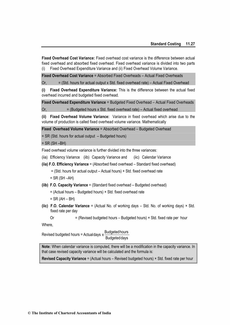
Standard Costing 11.27
Fixed Overhead Cost Variance: Fixed overhead cost variance is the difference between actual
fixed overhead and absorbed fixed overhead. Fixed overhead variance is divided into two parts
(i) Fixed Overhead Expenditure Variance and (ii) Fixed Overhead Volume Variance.
Fixed Overhead Cost Variance = Absorbed Fixed Overheads – Actual Fixed Overheads
Or, = (Std. hours for actual output x Std. fixed overhead rate) – Actual Fixed Overhead
(i) Fixed Overhead Expenditure Variance: This is the difference between the actual fixed
overhead incurred and budgeted fixed overhead.
Fixed Overhead Expenditure Variance = Budgeted Fixed Overhead – Actual Fixed Overheads
Or, = (Budgeted hours x Std. fixed overhead rate) – Actual fixed overhead
(ii) Fixed Overhead Volume Variance: Variance in fixed overhead which arise due to the
volume of production is called fixed overhead volume variance. Mathematically
Fixed Overhead Volume Variance = Absorbed Overhead – Budgeted Overhead
= SR (Std. hours for actual output – Budgeted hours)
= SR (SH –BH)
Fixed overhead volume variance is further divided into the three variances:
(iia) Efficiency Variance (iib) Capacity Variance and (iic) Calendar Variance
(iia) F.O. Efficiency Variance = (Absorbed fixed overhead – Standard fixed overhead)
= (Std. hours for actual output – Actual hours) × Std. fixed overhead rate
= SR (SH –AH)
(iib) F.O. Capacity Variance = (Standard fixed overhead – Budgeted overhead)
= (Actual hours – Budgeted hours) × Std. fixed overhead rate
= SR (AH – BH)
(iic) F.O. Calendar Variance = (Actual No. of working days – Std. No. of working days) × Std.
fixed rate per day
Or = (Revised budgeted hours – Budgeted hours) × Std. fixed rate per hour
Where,
Revised budgeted hours =Budgetedhours
Actualdays xBudgeteddays
Note: When calendar variance is computed, there will be a modification in the capacity variance. In
that case revised capacity variance will be calculated and the formula is:
Revised Capacity Variance = (Actual hours – Revised budgeted hours) × Std. fixed rate per hour
© The Institute of Chartered Accountants of India

11.28 Cost Accounting
Verification of formulae:
F.O. Cost Variance = F.O. Expenditure Variance + F.O. Volume Variance
F. O. Volume Variance = Efficiency Variance + Capacity Variance + Calendar Variance
Basic terms used in the computation of overhead variance
Standard overhead rate (per hour) = Budgeted Overhead
Budgeted hours
Or
Standard overhead rate (per unit) = Budgeted Overhead
Budgeted output in units
b
Note: Separate overhead rates will be computed for fixed and variable overheads.
Basic calculations before the computation of overhead variances:
The following basic calculation should be made before computing variances.
(i) When overhead rate per hour is used:
(a) Standard hours for actual output (SHAO)
SHAO = Budgeted Hours
ActualOutputBudgeted Output
×
b
(b) Absorbed (or Recovered) overhead = Std. hours for actual output × Std. overhead rate
per hour
(c) Standard overhead = Actual hours × Std. overhead rate per hour
(d) Budgeted overhead = Budgeted hours × Std. overhead rate per hour
(e) Actual overhead = Actual hours × Actual overhead rate per hour
(ii) When overhead rate per unit is used
(a) Standard output for actual hours (SOAH)
SOAH = Budgeted Output
Actual HoursBudgeted Hours
×
b
(b) Absorbed overhead = Actual output × Std. overhead rate per unit
(c) Standard overhead = Std. output for actual time × Std. overhead rate per unit
(d) Budgeted overhead = Budgeted output × Std. overhead rate per unit
© The Institute of Chartered Accountants of India

Standard Costing 11.29
(e) Actual overhead = Actual output × Actual overhead rate per unit
Overhead cost variance = Absorbed overhead – Actual overhead
OCV = (Std. hours for actual output × Std. overhead rate) – Actual
overhead
The following illustration shows how overhead expense rates are computed and variance analysed.
Illustration 9 (Calculation of production volume variance and overhead expense variance)
The overhead expense budget for a factory producing to a capacity of 200 units per month is
as follows:
Description of overhead Fixed cost
per unit in `
Variable cost per
unit in `
Total cost
per unit in `
Power and fuel 1,000 500 1,500
Repair and maintenance 500 250 750
Printing and stationary 500 250 750
Other overheads 1,000 500 1,500
` 3,000 ` 1,500 4,500
The factory has actually produced only 100 units in a particular month. Details of overheads
actually incurred have been provided by the accounts department and are as follows:
Description of overhead Actual cost
Power and fuel ` 4,00,000
Repair and maintenance ` 2,00,000
Printing and stationary ` 1,75,000
Other overheads ` 3,75,000
You are required to compute the production volume variance and the overhead expenses variance.
Solution:
Production volume variance
Standard fixed overheads per unit : ` 3,000 (Given)
Actual production : 100 units
Standard production (capacity) : 200 units
Unabsorbed units : 100 units (200 – 100 )
Production volume variance : ` 3,000 × 100 units
= ` 3,00,000 (Adverse)
© The Institute of Chartered Accountants of India

11.30 Cost Accounting
Overhead expenses variance
Standard fixed overheads for actual production : ` 6,00,000
Standard variable overheads for actual production : ` 1,500 × 100 units
= ` 1,50,000
Std total overheads for actual production : ` 7,50,000
Actual overheads : ` 11,50,000
Overhead expense variance : ` 4,00,000 (Adverse)
Illustration10 (Calculation of production volume variance and overhead expense
variance)
XYZ Company has established the following standards for factory overheads.
Variable overhead per unit: ` 10/-
Fixed overheads per month ` 1,00,000
Capacity of the plant 20,000 units per month.
The actual data for the month are as follows:
Actual overheads incurred ` 3,00,000
Actual output (units) 15,000 units
Required:
Calculate overhead variances viz :
(i) Production volume variance
(ii) Overhead expense variance
Solution:
Unutilised capacity : 20,000 units less 15,000 units
= 5,000 units
Std fixed overheads per unit = ` 5 per unit
Production volume variance = 5,000 units × ` 5
= ` 25,000 (Adverse)
Std variable overheads for actual production : ` 10 × 15,000 units
= ` 1,50,000
Std fixed overheads = ` 1,00,000
Total overheads on standards for actual production = ` 2,50,000
© The Institute of Chartered Accountants of India

Standard Costing 11.31
Actual overheads incurred = ` 3,00,000
Overhead expense variance = ` 50,000
Illustration 11 (Calculation of variable overhead variance, fixed overhead expenditure
and volume variance)
The following information was obtained from the records of a manufacturing unit using
standard costing system.
Standard Actual
Production 4,000 units 3,800 units
Working days 20 21
Fixed Overhead ` 40,000 ` 39,000
Variable Overhead 12,000 12,000
You are required to calculate the following overhead variance:
(a) Variable overhead variance
(b) Fixed overhead variances
(i) Expenditure variances
(ii) Volume variance
Solution:
(a) For Variable Overhead Variance:
Actual variable overhead = `12, 000
Standard variable overhead for production (Budgeted output × Std. variable overhead
rate per unit) = (12,000 ÷ 4,000) × 3,800
= `11, 400
Variable overhead variance: Standard variable overhead - Actual variable overhead
= `11, 400 – `12, 000
= 600 (A)
(b) For Fixed Overhead Variance:
Actual fixed overhead incurred = ` 39, 000
Budgeted fixed overhead for the period = ` 40, 000
Standard fixed overhead for production (Standard output for actual time × Standard Fixed
Overhead per unit)
= (`40, 000 ÷ 4,000 units) × 3,800 units = `38, 000.
© The Institute of Chartered Accountants of India

11.32 Cost Accounting
Variances:
(i) Fixed Overhead Expenditure Variances:
Budgeted fixed overhead – Actual fixed overhead
= `40, 000 – `39, 000 = 1,000 (F)
(ii) Fixed Overhead Volume Variance : Standard fixed overhead – Budgeted fixed overhead
= `38, 000 – `40, 000 = `2, 000 (A)
(iii) Fixed Overhead Variance : Standard fixed overhead – Actual fixed overhead
= `38, 000 – `39, 000 = `1, 000 (A)
Illustration12 (Calculation of Fixed overhead cost, expenditure and volume variance)
A company has a normal capacity of 120 machines, working 8 hours per day of 25 days in a
month. The fixed overheads are budgeted at `1, 44,000 per month. The standard time
required to manufacture one unit of product is 4 hours.
In April, 2012, the company worked 24 days of 840 machine hours per day and produced
5,305 units of output. The actual fixed overheads were `1, 42,000.
Compute:
(i) Expense variance
(ii) Volume variance
(iii) Total fixed overheads variance.
Solution
Working Notes:
Budget Actual
1. Working hours per month 24,000 20,160
2. Production units per month = (Budget 24,000 ÷ 4 hrs, Actual given) 6,000 5,305
3. Standard fixed overhead rate per unit = `1,44,000 ÷ 6,000 = ` 24
4. Standard fixed overhead rate per hour = `1,44,000 ÷ 24,000 = `6
5. Standard fixed overhead rate per day = `1,44,000 ÷ 25 = ` 5,760
Fixed Overhead Variances:
Actual Fixed overhead incurred = `1, 42,000 (given)
Budgeted fixed overhead for the period = `1, 44,000.
Standard fixed overhead for actual production (Standard output for actual time × Standard
Fixed Overhead per unit) = 5,305 × `24 = `1, 27,320.
© The Institute of Chartered Accountants of India

Standard Costing 11.33
Variances:
(i) F.O. Expenditure Variance = (Budgeted fixed overhead – Actual fixed overhead)
= 1, 44,000 – 1, 42,000 = ` 2, 000 (F)
(ii) Total Volume Variance = (Standard fixed overhead – Budgeted fixed overhead)
= 1, 27,320 – 1, 44,000 = `16, 680 (A)
(iii) Fixed overhead variance = (Standard fixed overhead – Actual Fixed overhead)
= 1, 27,320 – 1, 42,000 = `14, 680 (A)
Alternatively:
Expenditure Variance + Volume Variance = 2,000 (F) + 16,680 (A) = `14, 680 (A)
Illustration13 (calculation of Fixed overhead cost, expenditure and volume variance)
Following information is available from the records of a factory:
Budget Actual
Fixed overhead for June, 2012 `10,000 `12,000
Production in June, 2012 (units) 2,000 2,100
Standard time per unit (hours) 10 –
Actual hours worked in June – 21,000
Compute:
(i) Fixed overhead cost variance,
(ii) Expenditure variance,
(iii) Volume variance.
Solution:
For fixed overhead variances:
Actual F.O. incurred (given) `12,000
Budgeted F.O. for the period `10,000
Standard F.O. for production (Standard output for actual time × Standard Fixed Overhead per unit)
2,100 units × {`10,000 ÷ 2,000 units}
`10,500
(i) Fixed Overhead Variance = Standard F.O. – Actual F.O.
= ` 10,500 – `12,000
= `1,500 (A)
© The Institute of Chartered Accountants of India

11.34 Cost Accounting
(ii) F.O. Expenditure Variance = Budgeted F.O – Actual F.O.
= `10,000 – `12,000
= `2,000 (A)
(iii) F.O. Volume Variance = Standard F.O – Budgeted F.O.
= `10,500 – ` 10,000
= ` 500 (F)
Illustration 14 (Calculation of Fixed overhead variance and variable overhead variance)
XYZ Ltd. has furnished you the following information for the month of August, 2012:
Budget Actual
Output (units) 30,000 32,500
Hours 30,000 33,000
Fixed overhead ` 45,000 50,000
Variable overhead ` 60,000 68,000
Working days 25 26
Calculate overhead variances.
Solution:
Basic Calculations:
Standard hours per unit = unitsBudgeted
hoursBudgeted=
30,000
30,000= 1 hour
Std. hrs. for actual output = 32,500 units × 1 hr = 32,500
Standard overhead rate per hour = hoursBudgeted
overheadBudgeted
For fixed overhead = 45,000
30,000= `1.50 per hour
For variable overhead = 60,000
30,000= `2 per hour
Std. F.O. rate per day = `45,000 ÷ 25 days = `1,800
Recovered overhead = Std. hrs. for actual output × St. rate
For fixed overhead = 32,500 hrs. × `1.50 = `48,750
For variable overhead = 32,500 hrs. × `2 = `65,000
© The Institute of Chartered Accountants of India

Standard Costing 11.35
Standard overhead = Actual hours × Std. rate
For fixed overhead = 33,000 × 1.50 = `49,500
For variable overhead = 33,000 × 2 = `66,000
Revised budget hours = days Budgeted
hours Budgeted× Actual days
= 25
30,000× 26 = 31,200 hours
Revised budgeted overhead (for fixed overhead) = 31,200 × 1.50 = `46,800
Calculation of variances
Fixed Overhead Variances:
(i) F.O. cost Variance = Recovered Overhead – Actual Overhead
= 48,750 – 50,000
= `1,250 (A)
(ii) F.O. Expenditure Variance = Budgeted Overhead – Actual Overhead
= 45,000 – 50,000
= ` 5,000 (A)
(iii) F.O. Volume Variance = Recovered Overhead – Budgeted Overhead
= 48,750 – 45,000
= ` 3,750 (F)
(iv) F.O. Efficiency Variance = Recovered Overhead – Standard Overhead
= 48,750 – 49,500 = `750 (A)
(v) F.O. Capacity Variance = Standard Overhead- Revised Budgeted Overhead
= 49,500-46800 =` 2,700 (F)
(v) Calendar Variance =
−
Days
Budgeted
Days
Actual × St. rate per day.
= (26 – 25) × 1,800 = `1,800 (F)
Variable Overhead Variances
(i) V.O. Cost variance = Recovered Overhead – Actual Overhead
= 65,000 – 68,000 = ` 3,000 (A)
(ii) V.O. Expenditure Variance = Standard Overhead – Actual Overhead
= 66,000 – 68,000 = ` 2,000 (A)
© The Institute of Chartered Accountants of India

11.36 Cost Accounting
(iii) V.O. Efficiency Variance = Recovered Overhead – Standard Overhead
= 65,000 – 66,000 = `1,000 (A)
Check
(i) F.O. Cost Variance = Expenditure variance + Volume variance
1,250 (A) = 5,000 (A) + 3,750 (F)
(ii) F.O. Volume Variance = Variance
Efficiency+
Variance
Capacity+
Variance
Calendar
3,750 (F) = 750 (A) + 2,700 (F) + 1,800 (F)
(iii) V.O. Cost Variance = Expenditure Variance + Efficiency Variance
3,000 (A) = 2,000 (A) + 1,000 (A).
Illustration 15 (Calculation of fixed overhead volume, expenditure and cost variance)
S.V. Ltd. has furnished the following data:
Budget Actual, July (2012)
No. of working days 25 27
Production in units 20,000 22,000
Fixed overheads ` 30,000 ` 31,000
Budgeted fixed overhead rate is ` 1.00 per hour. In July, 2012, the actual hours worked were 31,500.
Calculate the following variances:
(i) Volume variance.
(ii) Expenditure variance.
(iii) Total overhead variance.
Solution:
For Fixed Overhead Variances
Actual fixed overhead incurred ` 31,000
Budgeted fixed overhead for the period 30,000
Standard fixed overhead for production (Standard output for actual time ×
Standard Fixed Overhead per unit) (` 30,000 ÷ 20,000 units) × 22,000
33,000
© The Institute of Chartered Accountants of India

Standard Costing 11.37
Computation of Variances:
(i) Fixed overhead expenditure variance:
= Budgeted fixed overhead – Actual fixed overhead
= `30,000 – `31,000 = ` 1,000 (A)
(ii) Fixed overhead volume variance:
= Standard fixed overhead – Budgeted fixed overhead
= `33,000 – ` 30,000 = ` 3,000 (F)
(iii) Fixed overhead variance :
= Standard fixed overhead – Actual fixed overhead
= `33,000 – ` 31,000 = ` 2,000 (F)
Illustration 16 (Calculation of fixed overhead volume, expenditure and cost variance)
The following data has been collected from the cost records of a unit for computing the various
fixed overhead variances for a period:
Number of budgeted working days 25
Budgeted man-hours per day 6,000
Output (budgeted) per man-hour (in units) 1
Fixed overhead cost as budgeted ` 1,50,000
Actual number of working days 27
Actual man-hours per day 6,300
Actual output per man-hour (in-units) 0.9
Actual fixed overhead incurred ` 1,56,000
Calculate fixed overhead variances:
(a) Expenditure Variance
(b) Volume Variance,
(c) Fixed Cost Variance.
Solution:
For Fixed overhead Variances:
Actual fixed overhead incurred = `1,56,000
Budgeted fixed overhead for the period = 1,50,000
© The Institute of Chartered Accountants of India
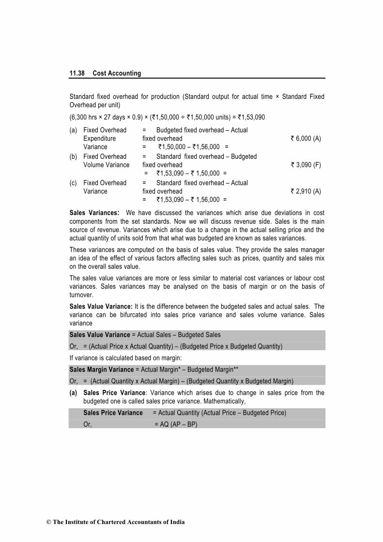
11.38 Cost Accounting
Standard fixed overhead for production (Standard output for actual time × Standard Fixed
Overhead per unit)
(6,300 hrs × 27 days × 0.9) × (`1,50,000 ÷ `1,50,000 units) = `1,53,090
(a) Fixed Overhead
Expenditure
Variance
= Budgeted fixed overhead – Actual
fixed overhead
= `1,50,000 – `1,56,000 =
` 6,000 (A)
(b) Fixed Overhead
Volume Variance
= Standard fixed overhead – Budgeted
fixed overhead
= `1,53,090 – ` 1,50,000 =
` 3,090 (F)
(c) Fixed Overhead
Variance
= Standard fixed overhead – Actual
fixed overhead
= `1,53,090 – ` 1,56,000 =
` 2,910 (A)
Sales Variances: We have discussed the variances which arise due deviations in cost
components from the set standards. Now we will discuss revenue side. Sales is the main
source of revenue. Variances which arise due to a change in the actual selling price and the
actual quantity of units sold from that what was budgeted are known as sales variances.
These variances are computed on the basis of sales value. They provide the sales manager
an idea of the effect of various factors affecting sales such as prices, quantity and sales mix
on the overall sales value.
The sales value variances are more or less similar to material cost variances or labour cost
variances. Sales variances may be analysed on the basis of margin or on the basis of
turnover.
Sales Value Variance: It is the difference between the budgeted sales and actual sales. The
variance can be bifurcated into sales price variance and sales volume variance. Sales
variance
Sales Value Variance = Actual Sales – Budgeted Sales
Or, = (Actual Price x Actual Quantity) – (Budgeted Price x Budgeted Quantity)
If variance is calculated based on margin:
Sales Margin Variance = Actual Margin* – Budgeted Margin**
Or, = (Actual Quantity x Actual Margin) – (Budgeted Quantity x Budgeted Margin)
(a) Sales Price Variance: Variance which arises due to change in sales price from the
budgeted one is called sales price variance. Mathematically,
Sales Price Variance = Actual Quantity (Actual Price – Budgeted Price)
Or, = AQ (AP – BP)
© The Institute of Chartered Accountants of India

Standard Costing 11.39
If variance is calculated based on margin:
Sales Margin Price Variance = Actual Quantity (Actual Margin – Budgeted Margin)
Or, = AQ (AM – BM)
(b) Sales Volume Variance: Variance which arises due to changes in actual sales quantity
from budgeted quantity is called sales volume variance. Mathematically,
Sale Volume Variance = Budgeted Price (Actual Quantity – Budgeted Quantity)
Or, = BP (AQ – BQ)
If variance is calculated based on margin:
Sales Margin Volume Variance = Budgeted Margin (Actual Quantity – Budgeted Quantity)
Or, = BM (AQ –BQ)
* Actual Margin = Actual Sales price per unit – Standard cost per unit
** Budgeted Margin = Budgeted Sales price per unit – Standard cost per unit
Illustration 17 (calculation of Sale value, price and volume variance)
Compute the sales variances from the following figures: -
Product Budgeted Budgeted Price Actual Actual
Quantity Quantity Price
(`) (`) (`)
A 2,000 2.50 2,400 3.00
B 1,500 5.00 1,400 4.50
C 1,000 7.50 1,200 7.00
D 500 10.00 400 10.50
Solution:
Basic calculation:
Product BQ x BP AQ x AP AQ x BP
A 2,000 x 2.50 = `5,000 2,400 x 3.00 = ` 7,200 2,400 x 2.50 = ` 6,000
B 1,500 x 5.00 = `7,500 1,400 x 4.50 = ` 6,300 1,400 x 5.00 = ` 7,000
C 1,000 x 7.50 = ` 7,500 1,200 x 7.00 = ` 8,400 1,200 x 7.50 = ` 9,000
D 500 x 10.00 = ` 5,000 400 x 10.50 = ` 4,200 400 x 10.00 = ` 4,000
Total ` 25,000 ` 26,100 ` 26,000
© The Institute of Chartered Accountants of India

11.40 Cost Accounting
Computation of Variances
Sales Price Variance = Actual quantity (Actual price – Budgeted price)
= (AQ x AP) – (AQ x BP)
= ` 26,100 – ` 26,000 = ` 100(F)
Sales Volume Variance = Budgeted price (Actual quantity – Budgeted quantity)
= (BP x AQ) – (BP x BQ)
= ` 26,000 – ` 25,000 = ` 1,000 (F)
Total variance = Actual sales – Budgeted sales
= ` 26,100 – ` 25,000 = `1,100 (F)
Illustration 18 (Calculation of Material Cost, price and usage variance)
J.K. Ltd. manufactures NXE by mixing three raw materials. For every batch of 100 kg. of NXE, 125
kg. of raw materials are used. In April, 2012, 60 batches were prepared to produce an output of
5,600 kg. of NXE. The standard and actual particulars for April, 2012, are as follows :
Raw Materials
Standard Actual Quantity of Raw Materials
Purchased Mix Price per kg. Mix Price per Kg.
(%) (`) (%) (`) (Kg.)
A 50 20 60 21 5,000
B 30 10 20 8 2,000
C 20 5 20 6 1,200
Calculate all variances.
Solution:
Actual material used = 125 kg × 60 = 7,500 kg.
Actual cost of actual material used (AQ × AR) (`)
A 60% 4,500 kg × `21 = 94,500
B 20% 1,500 kg × ` 8 = 12,000
C 20% 1,500 kg × ` 6 = 9,000
7,500 1,15,500
© The Institute of Chartered Accountants of India

Standard Costing 11.41
Standard cost of actual material used (AQ × SR) (`)
A 4,500 kg × `20 = 90,000
B 1,500 kg × `10 = 15,000
C 1,500 kg × ` 5 = 7,500
7,500 1,12,500
Standard cost of material, if it had been used in standard proportion (Standard
Proportion × Standard Rate) (`)
A 50% 3,750 kg × `20 = 75,000
B 30% 2,250 kg × `10 = 22,500
C 20% 1,500 kg × ` 5 = 7,500
7,500 1,05,000
Standard cost of production (SQ for actual production × SR)
Standard cost of output for 100 kg: (`)
A 62.50 kg × `20 = 1,250
B 37.50 kg × `10 = 375
C 25.00 kg × ` 5 = 125
125.00 1,750
Standard cost for output of 5,600 kg.
= 100
1,750kg × 5,600 kg. = ` 98,000
Material Price Variance = Standard cost of actual material used – Actual cost of actual
material used = `1,12,500 – `1,15,500 = ` 3,000 (A)
Material Usage Variance = Standard cost of production – Standard cost of actual material
used = ` 98,000 – `1,12,500 = `14,500 (A)
Note: Material Price Variance can be calculated at the time of purchase as well. In that case,
material variance will be as follows:
Actual cost of material used
A 5,000 kg × `21 = ` 1,05,000
B 2,000 kg × ` 8 = ` 16,000
© The Institute of Chartered Accountants of India

11.42 Cost Accounting
C 1,200 kg × ` 6 = ` 7,200
1,28,200
Standard cost of material used
A 5,000 kg × `20 = ` 1,00,000
B 2,000 kg × `10 = ` 20,000
C 1,200 kg × ` 5 = ` 6,000
1,26,000
Material Price variance (if calculated at the time of purchase)
= Standard cost of actual material used – Actual cost of actual material used
= `1,26,000 – `1,28,200 = ` 2,200 (A)
11.9 Preparation of Operating Statement under Standard Costing – Reporting of Variances
Computation of variances and their reporting is not the final step towards the control of various
elements of cost. It demands an analysis of variances from the side of the executives, to
ascertain the correct reasons for their occurrence.
After knowing the exact reasons, it becomes their responsibility to take necessary steps so as
to stop the reoccurrence of adverse variances in future.
To enhance the utility of such a reporting system it is necessary that such a system of
reporting should not only be prompt but should also facilitate the concerned managerial level
to take necessary steps. Variance reports should be prepared after keeping in view its ultimate
use and its periodicity.
Such reports should highlight the essential cost deviations and possibilities for their
improvements. The variance reports should give due regard to the following points:-
(i) The concerned executives should be informed about what the cost performance should
have been.
(ii) How close the actual cost performance is with reference to standard cost performance.
(iii) The analysis and causes of variances.
(iv) Reporting should be based on the principle of management by exception.
(v) The magnitude of variances should also be stated.
© The Institute of Chartered Accountants of India

Standard Costing 11.43
Standard cost reports: Standard cost reports showing the details of the variances are
prepared for control purposes. Two such reports are illustrated below:
Standard Costing Profit and Loss Report Month ________20________
Particulars Total(`) Dept. A (`) Dept.B (`) Dept. C (`)
Sales value
Less: Standard cost of sales
Standard profit
Add / Deduct variances:
Materials : Price
Usage
Labour : Rate of pay
Efficiency
Overhead : Expense
Production volume
Actual profit
(a) Standard Costing Profit & Loss statement: A standard costing profit and loss statement
will show the variance of each type under each element of cost department wise and is
illustrated as below:
The adverse variance may be shown in red or in parenthesis.
The following case study shall help you understand the mechanics of a standard costing system.
11.10 Accounting Procedure For Standard Cost
The standard cost operations can be recorded in the books of account. Two important
accounting procedures for standard costs are:-
(i) Single Plan: The main purpose of standard costing is cost control. To achieve this
purpose, the variances should be analysed according to their causes.
Analysis should be timely so that much time is not lost in taking corrective action
wherever needed. In the partial plan, variances are analysed at the end of period.
The single plan system envisages the posting of all items in the debit side of the work-in-
progress account at the standard cost leaving the credit side to represent the standard
cost of finished production and work-in-progress.
© The Institute of Chartered Accountants of India
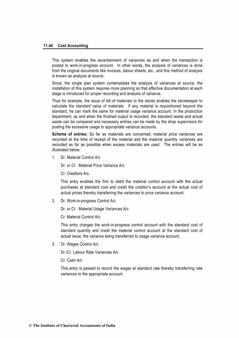
11.44 Cost Accounting
This system enables the ascertainment of variances as and when the transaction is
posted to work-in-progress account. In other words, the analysis of variances is done
from the original documents like invoices, labour sheets, etc., and this method of analysis
is known as analysis at source.
Since, the single plan system contemplates the analysis of variances at source, the
installation of this system requires more planning so that effective documentation at each
stage is introduced for proper recording and analysis of variance.
Thus for example, the issue of bill of materials to the stores enables the storekeeper to
calculate the standard value of materials. If any material is requisitioned beyond the
standard, he can mark the same for material usage variance account. In the production
department, as and when the finished output is recorded, the standard waste and actual
waste can be compared and necessary entries can be made by the shop supervisors for
posting the excessive usage to appropriate variance accounts.
Scheme of entries: So far as materials are concerned, material price variances are
recorded at the time of receipt of the material and the material quantity variances are
recorded as far as possible when excess materials are used. The entries will be as
illustrated below:
1. Dr. Material Control A/c
Dr. or Cr. Material Price Variance A/c
Cr. Creditors A/c.
This entry enables the firm to debit the material control account with the actual
purchases at standard cost and credit the creditor’s account at the actual cost of
actual prices thereby transferring the variances to price variance account.
2. Dr. Work-in-progress Control A/c
Dr. or Cr. Material Usage Variances A/c
Cr. Material Control A/c
This entry charges the work-in-progress control account with the standard cost of
standard quantity and credit the material control account at the standard cost of
actual issue, the variance being transferred to usage variance account.
3. Dr. Wages Control A/c
Dr./Cr. Labour Rate Variances A/c
Cr. Cash A/c
This entry is passed to record the wages at standard rate thereby transferring rate
variances to the appropriate account.
© The Institute of Chartered Accountants of India

Standard Costing 11.45
4. Dr. Work-in-progress Control A/c
Dr. or Cr. Overhead Expense Variances A/c
Cr. Overhead Expense Control A/c.
(ii) Partial plan: This system uses current standards in which the inventory will be valued at
current standard cost figure.
Under this method the work-in-progress account is charged at the actual cost of
production for the month and is credited with the standard cost of the month’s production
of finished product.
The closing balance of work-in-progress is also shown at standard cost. The balance
after making the credit entries represent the variance from standard for the month. The
analysis of the variance is done after the end of the month. This method is simple in
operation because variances are analysed after the end of month but may present
difficulties if the firm makes a variety of products.
Recapitulation :
(1) Current standards are used in both the systems.
(2) Under the partial plan, material stocks are carried at actual cost whereas the same are
carried out at standard cost under the single plan.
(3) The work-in-progress and finished goods are valued at standard cost under both the
methods.
(4) Computation of variances :
(a) In partial plan, material price variance is computed on material used in finished
goods and work-in-progress whereas in single plan it is computed on the material
quantity purchased.
(b) The partial plan is suitable where simple analysis of variance is sufficient at the end
of the period whereas the single plan is preferred if frequent detailed analysis of
variance is desired, as (a) the comparison of actual with standard cost of each
operation or operator or (b) the daily reporting of standard cost of excess material
used.
11.11 Disposition of Variances
There is no unanimity of opinion in regard to disposition of variances. The following are the
various methods:–
(a) Write off all variances to profit and loss account or cost of sales every month.
(b) Distribute the variance pro-rata to cost of sales, work-in-progress and finished good
stocks.
© The Institute of Chartered Accountants of India

11.46 Cost Accounting
(c) Write off quantity variance to profit and loss account but the price variances may be
spread over cost of sales, work-in-progress and finished goods stocks. The reason
behind apportioning price variances to inventories and cost of sales is that they represent
cost although they are described as variance.
11.12 Advantages and Criticism of Standard Costing
11.12.1 Advantages of Standard Costing: Following are the advantages of standard
costing.
(i) It serves as a basis for measuring operating performance and cost control. By setting
standards, proper classification and determination of variances, is possible. This serves
as a signal for prompt corrective action. This system provides for reporting on the
principle of exception. The basis of this principle is that only matters which are not
proceeding according to plan are reported upon. This enables the managers to
concentrate upon essential matters and leave the non-essentials to take care of
themselves. By using special forms, any excessive time taken, extra material used or
additional services consumed can be brought to light as part of the ordinary routine. In
other words, if the variances are negligible, it means that the performance is more or less
in accordance with the standards. Significant variances which warrant the attention of the
manager are brought to his knowledge.
(ii) It aids price fixing. Standard costing can be used to predict costs. Although actual cost
may vary from day to day, standard costs will remain stable over a period of time and,
where demand for a product is elastic, this information can be used as a basis for fixing
the selling price.
(iii) Introduction of standard costing facilitates evaluation of jobs and introduction of
incentives. Job values can be determined by the use of evaluation and scale of wages
fixed according to the responsibility involved in each job.
(iv) Standard costing facilitates the estimation of the cost of new products with greater accuracy.
(v) It serves as a basis for inventory valuation. Standard costs are used for inventory
valuation because actual costs are not typical and less clerical work is involved in
carrying standard value into inventory records than actual value. A further advantage of
this procedure is that material stock can be recorded in terms of quantities only.
(vi) Standard costing is also used for the measurement of profits. The question of correct
approach of calculating profit is very much related to stock valuation and to the methods
of dealing with the absorption of fixed overheads. Standard costing will eliminate any
variations in profit due to changes in the values of stock holding from period to period
and will thus provide a true basis for the measurement of profit.
© The Institute of Chartered Accountants of India

Standard Costing 11.47
(vii) Standard costing greatly aids business planning, budgeting and managerial decision
making. Standard costs being pre-determined costs, are particularly useful in planning
and budgeting.
(viii) Standard costing aids in standardisation of products, operations and processes. Since
standards are laid down for each product, its components, materials, operations,
processes etc., it improves the overall production efficiency and reduces costs.
(ix) It provides objectives and targets to be achieved by each level of management and
defines the responsibilities of departmental managers. Standard costs are pre-
determined on the basis of reasonable and achievable level of output. The departmental
head, therefore, comes to know what is expected of him and his level of performance in
comparison to the targets can be seen from the variance reports. Thus the system serves
as an incentive to the departmental head to achieve the targets set by the company.
(x) Standard costing sets a uniform basis for comparison of all elements of costs. Since care
is taken in setting standards, the standards become unchanging units of comparison. The
standard hour may be used as a basic unit to compare dissimilar products or processes.
(xi) The maximum use of working capital, plant facilities and current assets is assured
because wastage of materials and loss due to idle time are closely controlled.
11.12.2 Criticism of Standard Costing
The following are some of the criticism which may be leveled against the standard costing
system. The arguments have been suitably answered as stated against each by advocates of
the standard costing and hence they do not invalidate the usefulness of the system to
business enterprises.
(i) Variation in price: One of the chief problem faced in the operation of the standard costing
system is the precise estimation of likely prices or rate to be paid. The variability of prices is
so great that even actual prices are not necessarily adequately representative of cost. But the
use of sophisticated forecasting techniques should be able to cover the price fluctuation to
some extent. Besides this, the system provides for isolating uncontrollable variances arising
from variations to be dealt with separately.
(ii) Varying levels of output: If the standard level of output set for pre-determination of standard
costs is not achieved, the standard costs are said to be not realised. However, the statement
that the capacity utilisation cannot be precisely estimated for absorption of overheads may be
true only in some industries of jobbing type. In vast majority of industries, use of forecasting
techniques, market research, etc., help to estimate the output with reasonable accuracy and thus
the variation is unlikely to be very large. Prime cost will not be affected by such variation and,
moreover, variance analysis helps to measure the effects of idle time.
© The Institute of Chartered Accountants of India

11.48 Cost Accounting
(iii) Changing standard of technology: In case of industries that have frequent technological
changes affecting the conditions of production, standard costing may not be suitable. This
criticism does not affect the system of standard costing. Cost reduction and cost control is a
cardinal feature of standard costing because standards once set do not always remain stable.
They have to be revised.
(iv) Attitude of technical people: Technical people are accustomed to think of standards as
physical standards and, therefore, they will be misled by standard costs. Since technical
people can be educated to adopt themselves to the system through orientation courses, it is
not an insurmountable difficulty.
(v) Mix of products: Standard costing presupposes a pre-determined combination of
products both in variety and quantity. The mixture of materials used to manufacture the
products may vary in the long run but since standard costs are set normally for a short period,
such changes can be taken care of by revision of standards.
(vi) Level of Performance: Standards may be either too strict or too liberal because they may
be based on (a) theoretical maximum efficiency, (b) attainable good performance or (c)
average past performance. To overcome this difficulty the management should give thought to
the selection of a suitable type of standard. The type of standard most effective in the control
of costs is one which represents an attainable level of good performance.
(vii) Standard costs cannot possibly reflect the true value in exchange. If previous historical
costs are amended roughly to arrive at estimates for ad hoc purposes, they are not standard
costs in the strict sense of the term and hence they cannot also reflect true value in exchange.
In arriving at standard costs, however, the economic and technical factors, internal and
external, are brought together and analysed to arrive at quantities and prices which reflect
optimum operations. The resulting costs, therefore, become realistic measures of the
sacrifices involved.
(viii) Fixation of standards may be costly: It may require high order of skill and competency.
Small concerns, therefore, feel difficulty in the operation of such system.
11.13 Summary
Standard Costing: A technique which uses standards for costs and revenues for the
purposes of control through variance analysis.
Standard Price: A predetermined price fixed on the basis of a specification of a product
or service and of all factors affecting that price.
Standard Time: The total time in which task should be completed at standard
performance.
© The Institute of Chartered Accountants of India

Standard Costing 11.49
Variance: A divergence from the predetermined rates, expressed ultimately in money
value, generally used in standard costing and budgetary control systems.
Variance Analysis: The analysis of variances arising in standard costing system into
their constituent parts.
Revision Variance: It is the difference between the original standard cost and the
revised standard cost of actual production.
Basic Standard: A standard fixed for a fairly long period.
Current Standard: A standard fixed for a short period.
Estimated Cost : An estimate of what the cost is likely to be during a given period of time.
Ideal Cost : A cost which should be incurred during a period under ideal conditions.
Important Formulas
Material Variance :
Material Costs Variance = (Std. qty × Std. Price) – (Actual qty × Actual price)
Material Usage Variance = Std. price (Std. Qty. – Actual qty.)
Material Price Variance = Actual qty. (Std. price – Actual price)
Material Cost Variance = Material usage variance + Material price variance
Material Mix Variance = SP (RSQ – AQ)
Material Yield Variance = SP (SQ – RSQ)
Labour Variance :
Labour Cost Variance = (Std. time × Std. Rate) – (Actual time × Actual rate)
Labour Efficiency Variance = Std. rate (Std. time – Actual time)
Labour Rate Variance = Actual time (Std. rate – Actual rate)
Labour Idle Time Variance = Idle time x Std. rate
Labour Cost Variance = Labour Efficiency Variance + Labour Rate Variance
Labour Mix Variance = SR (RSH – AH)
Labour Yield Variance = SR (SH – RSH)
© The Institute of Chartered Accountants of India

11.50 Cost Accounting
Fixed Overhead Variances:
F.O. Cost Variance = Recovered Overhead – Actual Overhead
F.O. Expenditure Variance = Budgeted Overhead – Actual Overhead
F.O. Volume Variance = Recovered Overhead – Budgeted Overhead
F.O. Efficiency Variance = Recovered Overhead – Standard Overhead
F.O. Capacity Variance = Standard Overhead – Budgeted Overhead
F.O. Calendar Variance = SR (Actual no. of working days – Std. no. working days)
Variable Overhead Variances
V.O. Cost variance = Recovered Overhead – Actual Overhead
V.O. Expenditure Variance = Standard Overhead – Actual Overhead
V.O. Efficiency Variance = Recovered Overhead – Standard Overhead
Sales Variance :
Sales Price Variance: Actual Quantity of Sales (Actual price – Budgeted price)
Sales Volume Variance: Budgeted Price (Actual quantity – Budgeted quantity)
© The Institute of Chartered Accountants of India

12 Marginal Costing
Learning Objectives
When you have finished studying this chapter, you should be able to • Understand the difference between absorption costing and marginal costing • Understand the concept of contribution and contribution to sales ratio. • Understand the method of computation of break-even point, both mathematically and
also with the help of a graph. • Understand the basic limitations of break even analysis
12.1 Definitions
In order to appreciate the concept of marginal costing, it is necessary to study the definition of marginal costing and certain other terms associated with this technique. The important terms have been defined as follows: 1. Marginal Costing: The ascertainment of marginal cost and of the effect on profit of changes in volume or type of output by differentiating between fixed costs and variable costs. 2. Marginal Cost: The amount at any given volume of output by which aggregate variable costs are changed if the volume of output is increased by one unit. In practice this is measured by the total variable cost attributable to one unit. Marginal cost can precisely be the sum of prime cost and variable overhead. Marginal Cost = Variable Cost = Direct Labour + Direct Material + Direct Expenses + Variable Overheads Note: In this context a unit may be a single article, a batch of articles, an order, a stage of production capacity, a process or a department. It relates to the change in output in particular circumstances under consideration. 3. Direct Costing: Direct costing is the practice of charging all direct cost to operations, processes or products, leaving all indirect costs to be written off against profits in the period in which they arise. Under direct costing the stocks are valued at direct costs, i.e., costs whether fixed or variable which can be directly attributable to the cost units.
© The Institute of Chartered Accountants of India

12.2 Cost Accounting
4. Differential Cost: It may be defined as “the increase or decrease in total cost or the change in specific elements of cost that result from any variation in operations”. It represents an increase or decrease in total cost resulting out of: (a) producing or distributing a few more or few less of the products; (b) a change in the method of production or of distribution; (c) an addition or deletion of a product or a territory; and (d) selection of an additional sales channel. Differential cost, thus includes fixed and semi-variable expenses. It is the difference between the total costs of two alternatives. It is an ad-hoc cost determined for the purpose of choosing between competing alternatives, each with its own combination of income and costs. 5. Incremental Cost: It is defined as, “the additional costs of a change in the level or nature of activity”. As such for all practical purposes there is no difference between incremental cost and differential cost. However, from a conceptual point of view, differential cost refers to both incremental as well as decremental cost. Incremental cost and differential cost calculated from the same data will be the same. In practice, therefore, generally no distinction is made between differential cost and incremental cost. One aspect which is worthy to note is that incremental cost is not the same at all levels. Incremental cost between 50% and 60% level of output may be different from that which is arrived at between 80% and 90% level of output. Differential cost or incremental cost analysis deals with both short-term and long-term problems. This analysis is more useful when various alternatives or various capacity levels are being considered. (will be discussed in the next chapter i.e. Budgets and Budgetary Control) 6. Contribution: Contribution or the contributory margin is the difference between sales value and the marginal cost [Contribution (C) = Sales (S) – Variable Cost]. It is obtained by subtracting marginal cost from sales revenue of a given activity. It can also be defined as excess of sales revenue over the variable cost. The contribution concept is based on the theory that the profit and fixed expenses of a business is a ‘joint cost’ which cannot be equitably apportioned to different segments of the business. In view of this difficulty the contribution serves as a measure of efficiency of operations of various segments of the business. The contribution forms a fund for fixed expenses and profit as illustrated below: Example: Variable Cost = ` 50,000, Fixed Cost = ` 20,000, Selling Price = ` 80,000
Contribution = Selling Price – Variable Cost
= ` 80,000 – ` 50,000 = ` 30,000
Profit = Contribution – Fixed Cost
= ` 30,000 – ` 20,000 = ` 10,000
Since, contribution exceeds fixed cost; the profit is of the magnitude of ` 10,000. Suppose the
© The Institute of Chartered Accountants of India

Marginal Costing 12.3
fixed cost is ` 40,000 then the position shall be: Contribution – Fixed cost = Profit or, =` 30,000 – ` 40,000 = -` 10,000 The amount of ` 10,000 represent extent of loss since the fixed costs are more than the contribution. At the level of fixed cost of ` 30,000, there shall be no profit and no loss. 7. Key Factor: Key factor or Limiting factor is a factor which at a particular time or over a period limits the activities of an undertaking. It may be the level of demand for the products or services or it may be the shortage of one or more of the productive resources, e.g., labour hours, available plant capacity, raw material’s availability etc. Examples of Key Factors or Limiting Factors are: (a) Shortage of raw material. (b) Shortage of labour. (c) Plant capacity available. (d) Sales capacity available. (e) Cash availability.
12.2 Characteristics of Marginal Costing
The technique of marginal costing is based on the distinction between product costs and period costs. Only the variables costs are regarded as the costs of the products while the fixed costs are treated as period costs which will be incurred during the period regardless of the volume of output. The main characteristics of marginal costing are as follows: 1. All elements of cost are classified into fixed and variable components. Semi-variable
costs are also analyzed into fixed and variable elements. 2. The marginal or variable costs (as direct material, direct labour and variable factory
overheads) are treated as the cost of product. 3. Under marginal costing, the value of finished goods and work–in–progress is also
comprised only of marginal costs. Variable selling and distribution are excluded for valuing these inventories. Fixed costs are not considered for valuation of closing stock of finished goods and closing WIP.
4. Fixed costs are treated as period costs and are charged to profit and loss account for the period for which they are incurred.
5. Prices are determined with reference to marginal costs and contribution margin. 6. Profitability of departments and products is determined with reference to their
contribution margin.
© The Institute of Chartered Accountants of India

12.4 Cost Accounting
12.3 Facts about Marginal Costing
Some of the facts about marginal costing are depicted below
Not a distinct method: Marginal costing is not a distinct method of costing like job costing, process costing, operating costing, etc., but a special technique used for managerial decision making. Marginal costing is used to provide a basis for the interpretation of cost data to measure the profitability of different products, processes and cost centres in the course of decision making. It can, therefore, be used in conjunction with the different methods of costing such as job costing, process costing, etc., or even with other techniques such as standard costing or budgetary control.
Cost Ascertainment: In marginal costing, cost ascertainment is made on the basis of the nature of cost. It gives consideration to behaviour of costs. In other words, the technique has developed from a particular conception and expression of the nature and behaviour of costs and their effect upon the profitability of an undertaking.
Decision Making: In the orthodox or total cost method, as opposed to marginal costing method, the classification of costs is based on functional basis. Under this method the total cost is the sum total of the cost of direct material, direct labour, direct expenses, manufacturing overheads, administration overheads, selling and distribution overheads. In this system, other things being equal, the total cost per unit will remain constant only when the level of output or mixture is the same from period to period. Since these factors are continually fluctuating, the actual total cost will vary from one period to another. Thus, it is possible for the costing department to say one day that an item costs `20 and the next day it costs `18. This situation arises because of changes in volume of output and the peculiar behaviour of fixed expenses included in the total cost. Such fluctuating manufacturing activity, and consequently the variations in the total cost from period to period or even from day to day, poses a serious problem to the management in taking sound decisions. Hence, the application of marginal costing has been given wide recognition in the field of decision making.
© The Institute of Chartered Accountants of India

Marginal Costing 12.5
12.4 Distinction between Marginal and Absorption Costing
The distinctions in these two techniques are illustrated by the following diagrams:
Fig. 12.1 Absorption Costing Approach
Fig. .2 Marginal Costing Approach
Direct materials Direct labour
Variable factory overhead
Fixed factory overhead
Charged to cost of goods produced
Charged as expenses when goods are sold
All selling and adm. overhead
Charged as expenses when
incurred
Direct materials
Direct labour
Variable factory overhead
Charged to cost of goods produced
Charged as expenses when goods are sold
Fixed factory overhead and all selling and adm.
overhead
Charged as expenses when
incurred
© The Institute of Chartered Accountants of India

12.6 Cost Accounting
12.4.1 The main points of distinction between marginal costing and absorption costing are as below:
Marginal costing Absorption costing
1. Only variable costs are considered for product costing and inventory valuation.
Both fixed and variable costs are considered for product costing and inventory valuation.
2. Fixed costs are regarded as period costs. The Profitability of different products is judged by their P/V ratio.
Fixed costs are charged to the cost of production. Each product bears a reasonable share of fixed cost and thus the profitability of a product is influenced by the apportionment of fixed costs.
3. Cost data presented highlight the total contribution of each product.
Cost data are presented in conventional pattern. Net profit of each product is determined after subtracting fixed cost along with their variable costs.
4. The difference in the magnitude of opening stock and closing stock does not affect the unit cost of production.
The difference in the magnitude of opening stock and closing stock affects the unit cost of production due to the impact of related fixed cost.
5. In case of marginal costing the cost per unit remains the same, irrespective of the production as it is valued at variable cost
In case of absorption costing the cost per unit reduces, as the production increases as it is fixed cost which reduces, whereas, the variable cost remains the same per unit.
12.4.2 Difference in profit under Marginal and Absorption costing: The above two approaches will compute the different profit because of the difference in the stock valuation. This difference is explained as follows in different circumstances. 1. No opening and closing stock: In this case, profit / loss under absorption and marginal
costing will be equal. 2. When opening stock is equal to closing stock: In this case, profit / loss under two
approaches will be equal provided the fixed cost element in both the stocks is same amount.
3. When closing stock is more than opening stock: In other words, when production during a period is more than sales, then profit as per absorption approach will be more than that by marginal approach. The reason behind this difference is that a part of fixed overhead included in closing stock value is carried forward to next accounting period.
4. When opening stock is more than the closing stock: In other words when production is less than the sales, profit shown by marginal costing will be more than that shown by
© The Institute of Chartered Accountants of India

Marginal Costing 12.7
absorption costing. This is because a part of fixed cost from the preceding period is added to the current year’s cost of goods sold in the form of opening stock.
12.4.3 Comparison between Direct Costing and Marginal Costing: In general, the terms marginal costing and direct costing are used as synonymous. However, direct costing differs from marginal costing in that some fixed costs considered direct are charged to operations, processes or products, whereas in marginal costing only variable costs are considered. Marginal costing is mainly concerned with providing of information to management to assist in decision making and for exercising control. Marginal costing is considered to be a technique with a broader meaning than direct costing. Marginal costing is also known as ‘variable costing’ or ‘out of pocket costing’.
12.4.4 Absorption Costing:
In absorption costing the classification of expenses is based on functional basis whereas in marginal costing it is based on the nature of expenses.
In absorption costing, the fixed expenses are distributed over products on absorption costing basis that is, based on a pre-determined level of output. Since fixed expenses are constant, such a method of recovery will lead to over or under-recovery of expenses depending on the actual output being greater or lesser than the estimate used for recovery. This difficulty will not arise in marginal costing because the contribution is used as a fund for meeting fixed expenses.
The presentation of information to management under the two costing techniques is as under: Income Statement (Absorption costing)
(`)
Sales XXXXX
Production Costs:
Direct material consumed XXXXX
Direct labour cost XXXXX
Variable manufacturing overhead XXXXX
Fixed manufacturing overhead XXXXX
Cost of Production XXXXX
Add: Opening stock of finished goods XXXXX
(Value at cost of previous period’s production)
XXXXX
Less: Closing stock of finished goods XXXXX
(Value at production cost of current period) .
Cost of Goods Sold XXXXX
© The Institute of Chartered Accountants of India
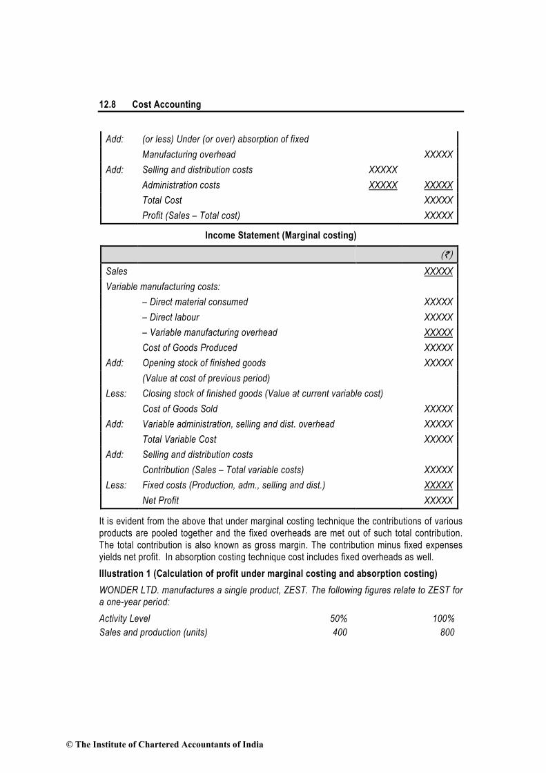
12.8 Cost Accounting
Add: (or less) Under (or over) absorption of fixed
Manufacturing overhead XXXXX
Add: Selling and distribution costs XXXXX
Administration costs XXXXX XXXXX
Total Cost XXXXX
Profit (Sales – Total cost) XXXXX
Income Statement (Marginal costing)
(`)
Sales XXXXX
Variable manufacturing costs:
– Direct material consumed XXXXX
– Direct labour XXXXX
– Variable manufacturing overhead XXXXX
Cost of Goods Produced XXXXX
Add: Opening stock of finished goods XXXXX
(Value at cost of previous period)
Less: Closing stock of finished goods (Value at current variable cost)
Cost of Goods Sold XXXXX
Add: Variable administration, selling and dist. overhead XXXXX
Total Variable Cost XXXXX
Add: Selling and distribution costs
Contribution (Sales – Total variable costs) XXXXX
Less: Fixed costs (Production, adm., selling and dist.) XXXXX
Net Profit XXXXX
It is evident from the above that under marginal costing technique the contributions of various products are pooled together and the fixed overheads are met out of such total contribution. The total contribution is also known as gross margin. The contribution minus fixed expenses yields net profit. In absorption costing technique cost includes fixed overheads as well. Illustration 1 (Calculation of profit under marginal costing and absorption costing)
WONDER LTD. manufactures a single product, ZEST. The following figures relate to ZEST for
a one-year period:
Activity Level 50% 100%
Sales and production (units) 400 800
© The Institute of Chartered Accountants of India

Marginal Costing 12.9
` lakhs ` lakhs
Sales 8.00 16.00
Production costs:
Variable 3.20 6.40
Fixed 1.60 1.60
Selling and administration costs:
Variable 1.60 3.20
Fixed 2.40 2.40
The normal level of activity for the year is 800 units. Fixed costs are incurred evenly
throughout the year, and actual fixed costs are the same as budgeted. There were no stocks
of ZEST at the beginning of the year.
In the first quarter, 220 units were produced and 160 units were sold.
Required:
(a) What would be the fixed production costs absorbed by ZEST if absorption costing is
used?
(b) What would be the under/over-recovery of overheads during the period?
(c) What would be the profit using absorption costing?
(d) What would be the profit using marginal costing?
Solution
(a) Fixed production costs absorbed: (`)
Budgeted fixed production costs 1,60,000 Budgeted output (normal level of activity 800 units) Therefore, the absorption rate :1,60,000/800 = ` 200 per unit During the first quarter, the fixed production cost absorbed by ZEST would be (220 units × ` 200) 44,000 (b) Under /over-recovery of overheads during the period: (`)
Actual fixed production overhead 40,000 (1/4 of ` 1,60,000) Absorbed fixed production overhead 44,000 Over-recovery of overheads 4,000 (c) Profit for the Quarter (Absorption Costing) (`) (`)
Sales revenue (160 units × ` 2,000) : (A) 3,20,000 Less: Production costs
© The Institute of Chartered Accountants of India

12.10 Cost Accounting
Variable (220 units × ` 800) 1,76,000 Fixed overheads absorbed (220 units × ` 200) 44,000 Total (220 units × ` 1,000) 2,20,000 Less: Closing stock (60 units × ` 1,000) (60,000) Production cost of 160 units 1,60,000 Variable sales & admn. costs (160 units × ` 400) 64,000 Fixed selling & admn. costs (1/4 of ` 2,40,000) 60,000 Total cost of sales of 160 units : (B) 2,84,000 Unadjusted profit : {(A) – (B)} 36,000 Add: Overheads over absorbed 4,000
Actual profit 40,000 (d) Profit for the Quarter (Marginal Costing) (`) (`)
Sales revenue (160 units × ` 2,000) : (A) 3,20,000 Variable production costs (220 units × ` 800) 1,76,000 Less: Closing stock (60 units × ` 800) (48,000) Variable production cost of 160 units 1,28,000 Add: Variable selling & admn. costs 64,000 Total variable cost of sales of 160 units : (B) 1,92,000 Contribution : {(A) – (B)} 1,28,000 Less: Fixed production cost incurred 40,000
Fixed selling & admn. costs incurred 60,000 1,00,000 Actual profit 28,000
Illustration 2 (Reasons for difference in profit under marginal and absorption costing)
XYZ Ltd. has a production capacity of 2,00,000 units per year. Normal capacity utilisation is
reckoned as 90%. Standard variable production costs are `11 per unit. The fixed costs are
`3,60,000 per year. Variable selling costs are `3 per unit and fixed selling costs are `2,70,000
per year. The unit selling price is `20.
In the year just ended on 30th June, 2014, the production was 1,60,000 units and sales were
1,50,000 units. The closing inventory on 30th June was 20,000 units. The actual variable
production costs for the year were ` 35,000 higher than the standard.
(i) Calculate the profit for the year
(a) by absorption costing method and
© The Institute of Chartered Accountants of India

Marginal Costing 12.11
(b) by marginal costing method.
(ii) Explain the difference in the profits. Solution :
Income Statement (Absorption Costing)
for the year ending 30th June 2014
(`) (`)
Sales (1,50,000 units @ `20) 30,00,000 Production Costs : Variable (1,60,000 units @ `11) 17,60,000 Add :Increase 35,000 17,95,000 Fixed (1,60,000 units @ `2*) 3,20,000
Cost of Goods Produced 21,15,000 Add :Opening stock (10,000 units @ `13)* 1,30,000 22,45,000
Less :Closing stock 21,15,000 20,000 units1,60,000 units
×
`
units
2,64,375
Cost of Goods Sold 19,80,625 Add :Under absorbed fixed production overhead (3,60,000 – 3,20,000) 40,000 20,20,625 Add :Non-production costs : Variable selling costs (1,50,000 units @ `3) 4,50,000 Fixed selling costs 2,70,000 Total cost 27,40,625 Profit (Sales – Total Cost) 2,59,375
* Working Notes :
1. Fixed production overhead are absorbed at a pre-determined rate based on normal capacity, i.e. `3,60,000 ÷ 1,80,000 units = ` 2.
2. Opening stock is 10,000 units, i.e., 1,50,000 units + 20,000 units – 1,60,000 units. It is valued at `13 per unit, i.e., `11 + `2 (Variable + fixed).
© The Institute of Chartered Accountants of India

12.12 Cost Accounting
Income Statement (Marginal Costing)
for the year ended 30th June, 2014
(`) (`)
Sales (1,50,000 units @ `20) 30,00,000 Variable production cost (1,60,000 units @ `11 + `35,000) 17,95,000 Variable selling cost (1,50,000 units @ `3) 4,50,000 22,45,000 Add : Opening Stock (10,000 units @ `11) 1,10,000
23,55,000
Less : Closing stock 17,95,000 20,000 units1,60,000
×
`
units
2,24,375
Variable cost of goods sold 21,30,625 Contribution (Sales – Variable cost of goods sold) 8,69,375 Less : Fixed cost – Production 3,60,000 – Selling 2,70,000 6,30,000 Profit 2,39,375
Reasons for Difference in Profit: (`)
Profit as per absorption costing 2,59,375 Add :Op. stock under –valued in marginal costing (`1,30,000 – 1,10,000) 20,000 2,79,375 Less :Cl. Stock under –valued in marginal closing (`2,64,375 – 2,24,375) 40,000 Profit as per marginal costing 2,39,375
12.5 Advantages and Limitations of Marginal Costing
Advantages
1. Simplified Pricing Policy: The marginal cost remains constant per unit of output whereas the fixed cost remains constant in total. Since marginal cost per unit is constant from period to period within a short span of time, firm decisions on pricing policy can be taken. If fixed cost is included, the unit cost will change from day to day depending upon the volume of output. This will make decision making task difficult.
2. Proper recovery of Overheads: Overheads are recovered in costing on the basis of pre-determined rates. If fixed overheads are included on the basis of pre-determined rates, there will be under- recovery of overheads if production is less or if overheads are
© The Institute of Chartered Accountants of India

Marginal Costing 12.13
more. There will be over- recovery of overheads if production is more than the budget or actual expenses are less than the estimate. This creates the problem of treatment of such under or over-recovery of overheads. Marginal costing avoids such under or over recovery of overheads.
3. Shows Realistic Profit: Advocates of marginal costing argues that under the marginal costing technique, the stock of finished goods and work-in-progress are carried on marginal cost basis and the fixed expenses are written off to profit and loss account as period cost. This shows the true profit of the period.
4. How much to produce: Marginal costing helps in the preparation of break-even analysis which shows the effect of increasing or decreasing production activity on the profitability of the company.
5. More control over expenditure: Segregation of expenses as fixed and variable helps the management to exercise control over expenditure. The management can compare the actual variable expenses with the budgeted variable expenses and take corrective action through analysis of variances.
6. Helps in Decision Making: Marginal costing helps the management in taking a number of business decisions like make or buy, discontinuance of a particular product, replacement of machines, etc.
7. Short term profit planning: It helps in short term profit planning by B.E.P charts. Limitations
1. Difficulty in classifying fixed and variable elements: It is difficult to classify exactly the expenses into fixed and variable category. Most of the expenses are neither totally variable nor wholly fixed. For example, various amenities provided to workers may have no relation either to volume of production or time factor.
2. Dependence on key factors: Contribution of a product itself is not a guide for optimum profitability unless it is linked with the key factor.
3. Scope for Low Profitability: Sales staff may mistake marginal cost for total cost and sell at a price; which will result in loss or low profits. Hence, sales staff should be cautioned while giving marginal cost.
4. Faulty valuation: Overheads of fixed nature cannot altogether be excluded particularly in large contracts, while valuing the work-in- progress. In order to show the correct position fixed overheads have to be included in work-in-progress.
5. Unpredictable nature of Cost: Some of the assumptions regarding the behaviour of various costs are not necessarily true in a realistic situation. For example, the assumption that fixed cost will remain static throughout is not correct. Fixed cost may change from one period to another. For example salaries bill may go up because of annual increments or due to change in pay rate etc. The variable costs do not remain
© The Institute of Chartered Accountants of India

12.14 Cost Accounting
constant per unit of output. There may be changes in the prices of raw materials, wage rates etc. after a certain level of output has been reached due to shortage of material, shortage of skilled labour, concessions of bulk purchases etc.
6. Marginal costing ignores time factor and investment: The marginal cost of two jobs may be the same but the time taken for their completion and the cost of machines used may differ. The true cost of a job which takes longer time and uses costlier machine would be higher. This fact is not disclosed by marginal costing.
7. Understating of W-I-P: Under marginal costing stocks and work in progress are understated.
12.6 Cost-Volume-Profit Analysis
Meaning: It is a managerial tool showing the relationship between various ingredients of profit planning viz., cost, selling price and volume of activity. As the name suggests, cost volume profit (CVP) analysis is the analysis of three variables cost, volume and profit. Such an analysis explores the relationship between costs, revenue, activity levels and the resulting profit. It aims at measuring variations in cost and volume. Assumptions:
1. Changes in the levels of revenues and costs arise only because of changes in the number of product (or service) units produced and sold – for example, the number of television sets produced and sold by Sony Corporation or the number of packages delivered by Overnight Express. The number of output units is the only revenue driver and the only cost driver. Just as a cost driver is any factor that affects costs, a revenue driver is a variable, such as volume, that causally affects revenues.
2. Total costs can be separated into two components; a fixed component that does not vary with output level and a variable component that changes with respect to output level. Furthermore, variable costs include both direct variable costs and indirect variable costs of a product. Similarly, fixed costs include both direct fixed costs and indirect fixed costs of a product
3. When represented graphically, the behaviours of total revenues and total costs are linear (meaning they can be represented as a straight line) in relation to output level within a relevant range (and time period).
4. Selling price, variable cost per unit, and total fixed costs (within a relevant range and time period) are known and constant.
5. The analysis either covers a single product or assumes that the proportion of different products when multiple products are sold will remain constant as the level of total units sold changes.
© The Institute of Chartered Accountants of India

Marginal Costing 12.15
6. All revenues and costs can be added, subtracted, and compared without taking into account the time value of money. (Refer to the FM study material for a clear understanding of time value of money).
Importance
It provides the information about the following matters: 1. The behavior of cost in relation to volume. 2. Volume of production or sales, where the business will break-even. 3. Sensitivity of profits due to variation in output. 4. Amount of profit for a projected sales volume. 5. Quantity of production and sales for a target profit level. Impact of various changes on profit:
An understanding of CVP analysis is extremely useful to management in budgeting and profit planning. It elucidates the impact of the following on the net profit: (i) Changes in selling prices,
(ii) Changes in volume of sales,
(iii) Changes in variable cost,
(iv) Changes in fixed cost.
12.6.1 Marginal Cost Equation: The contribution theory explains the relationship between the variable cost and selling price. It tells us that selling price minus variable cost of the units sold is the contribution towards fixed expenses and profit. If the contribution is equal to fixed expenses, there will be no profit or loss and if it is less than fixed expenses, loss is incurred. Since the variable cost varies in direct proportion to output, therefore if the firm does not produce any unit, the loss will be there to the extent of fixed expenses. These points can be described with the help of following marginal cost equation: S -V = C = F ± P Where, S = Selling price per unit, V = Variable cost per unit, C – Contribution, F = Fixed Cost, P = Profit/Loss Marginal Cost Statement (`)
Sales xxxx Less: Variable Cost xxxx Contribution xxxx Less: Fixed Cost xxxx Profit xxxx
© The Institute of Chartered Accountants of India

12.16 Cost Accounting
12.6.2 Contribution to Sales Ratio (Profit Volume Ratio or P/V ratio)
This ratio is usually expressed in percentage.
ContributionP / V Ratio 100Sales
= × or, P/V Ratio = Change in contribution / ProfitChange in sales
100×
A higher contribution to sales ratio implies that the rate of growth of contribution is faster than that of sales. This is because, once the breakeven point is reached, profits shall grow at a faster rate when compared to a product with a lesser contribution to sales ratio. By transposition, we have derived the following equations: (i) C = S × P/V ratio
(ii) S = CP / VRatio
12.6.3 Break-Even Analysis: Break-even analysis is a generally used method to study the CVP analysis. This technique can be explained in two ways: (i) In narrow sense it is concerned with computing the break-even point. At this point of
production level and sales there will be no profit and loss i.e. total cost is equal to total sales revenue.
(ii) In broad sense this technique is used to determine the possible profit/loss at any given level of production or sales.
12.7 Methods of Break -Even Analysis
Break even analysis may be conducted by the following two methods: (i) Algebraic computations (ii) Graphic presentations
12.8 Algebraic Calculations
12.8.1 Breakeven Point: The word contribution has been given its name because of the fact that it literally contributes towards the recovery of fixed costs and the making of profits. The contribution grows along with the sales revenue till the time it just covers the fixed cost. This point where neither profits nor losses have been made is known as a break-even point. This implies that in order to break even the amount of contribution generated should be exactly equal to the fixed costs incurred. Hence, if we know how much contribution is generated from each unit sold we shall have sufficient information for computing the number of units to be sold in order to break even. Mathematically,
© The Institute of Chartered Accountants of India

Marginal Costing 12.17
Break- even point in units = unit per onContributicosts Fixed
Example 1: of a company (ABC Ltd) manufacturing a single product, incurring variable costs of ` 300 per unit and fixed costs of ` 2, 00,000 per month. If the product sells for ` 500 per unit, the breakeven point shall be calculated as follows;
Break- even point in units = Fixed costsContribution per unit
= `
`
2,00,000200
= 1,000 units
Break- even points (in Rupees) = Total fixedcostContribution
× Sales
Break- even point (in Rupees) = Total fixedcost
P / V Ratio
12.8.2 Cash Break-even point: When break-even point is calculated only with those fixed costs which are payable in cash, such a break-even point is known as cash break-even point. This means that depreciation and other non-cash fixed costs are excluded from the fixed costs in computing cash break-even point. Its formula is –
Cash break- even point = unit per onContributi
costs fixed Cash
Illustration 3 (Calculation of BEP and sales)
You are given the following particulars calculate:
(a) Break-even point
(b) Sales to earn a profit of ` 20,000
i. Fixed cost ` 1,50,000
ii. Variable cost ` 15 per unit
iii. Selling price is ` 30 per unit
Solution:
(a) B.E.P = Fixed Cost / Contribution per unit* = `1,50,000 ÷ `15 = 10,000 Units * (Contribution per unit = Sales per unit – Variable cost per unit = ` 30 - `15)
(b) Sales to earn a Profit of ` 20,000 = (FC + Desired Profit)/ Contribution per unit x S.P. = (`1,50,000 + `20,000) ÷ 15 × 30 = `1,70,000 ÷ 15 × 30
© The Institute of Chartered Accountants of India

12.18 Cost Accounting
= ` 3,40,000 or, 1,70,000 1,70,000 3,40,000P / V Ratio 50%
= =` `
`
PV Ratio = 100SalesonContributi
×
Illustration 4 (Treatment of commission in computing sales price and calculation of
Break Even Point)
A Chinese soft drink company is planning to establish a subsidiary company in India to
produce mineral water. Based on the estimated annual sales of 40,000 bottles of the mineral
water, cost studies produced the following estimates for the Indian subsidiary:
Total annual costs Percent of Total Annual Cost which is variable
Material 2,10,000 100%
Labour 1,50,000 80%
Factory Overheads 92,000 60%
Administration Expenses 40,000 35%
The Indian production will be sold by manufacturer’s representatives who will receive a
commission of 8% of the sale price. No portion of the Chinese office expenses is to be
allocated to the Indian subsidiary. You are required to
(i) Compute the sale price per bottle to enable the management to realize an estimated 10%
profit on sale proceeds in India.
(ii) Calculate the break-even point in Rupee sales as also in number of bottles for the Indian
subsidiary on the assumption that the sale price is ` 14 per bottle.
Solution:
(i) Computation of Sale Price Per Bottle
Output: 40,000 Bottles (`)
Variable Cost: Material 2,10,000 Labour (`1,50,000 × 80%) 1,20,000 Factory Overheads (`92,000 × 60%) 55,200 Administrative Overheads (`40,000 × 35%) 14,000 Commission (8% on `6,00,000) (W.N.-1) 48,000
© The Institute of Chartered Accountants of India

Marginal Costing 12.19
Fixed Cost: Labour (`1,50,000 × 20%) 30,000 Factory Overheads (`92,000 × 40%) 36,800 Administrative Overheads (`40,000 × 65%) 26,000
Total Cost 5,40,000 Profit (W.N.-1) 60,000 Sales Proceeds (W.N.-1) 6,00,000
Sales Price per bottle 6,00,00040,000Bottles
` 15
(ii) Calculation of Break-even Point Sales Price per Bottle = `14
Variable Cost per Bottle = 4,44,000 (W.N.- 2)40,000Bottles
`
= `11.10 Contribution per Bottle = `14 − `11.10 = `2.90 Break -even Point
(in number of Bottles) = Fixed CostsContribution per Bottle
= 92,800 = 32,000Bottles2.90
`
` Break- even Point (in Sales Value) = 32,000 Bottles × `14 = `4,48,000 Working Note
W.N.-1
Let the Sales Price be ‘x’
Commission = 8x100
Profit = 10x100
© The Institute of Chartered Accountants of India

12.20 Cost Accounting
x = 4,92,000 + 8x 10x+100 100
100x - 8x - 10x = 4,92,00,000 82x = 4,92,00,000 x = 4,92,00,000 / 82 = `6,00,000
W.N.-2 Total Variable Cost (`)
Material 2,10,000 Labour 1,20,000 Factory Overheads 55,200 Administrative Overheads 14,000 Commission [(40,000 Bottles × `14) × 8%] 44,800 4,44,000
Illustration 5 (Calculation of selling price)
If P/V ratio is 60% and the Marginal cost of the product is ` 20. What will be the selling price?
Solution:
Variable Cost = 100 – P/V Ratio = 100 – 60 = 40
If Variable cost is 40, then selling price = 100 If Variable cost is 20, then selling price = (100/40) × 20 = ` 50 Illustration 6 (Calculation of capacity sales)
The ratio of variable cost to sales is 70%. The break-even point occurs at 60% of the capacity
sales. Find the capacity sales when fixed costs are ` 90,000. Also compute profit at 75% of
the capacity sales.
Solution:
Variable cost to sales = 70%, Contribution to sales = 30%, Or P/V Ratio 30% We know that: BES × P/V Ratio = Fixed Cost BES × 0.30 = ` 90,000 Or BES = ` 3,00,000 It is given that break-even occurs at 60% capacity. Capacity sales = ` 3,00,000 ÷ 0.60 = ` 5,00,000
© The Institute of Chartered Accountants of India

Marginal Costing 12.21
Computation of profit of 75% Capacity 75% of capacity sales (i.e. ` 5,00,000 × 0.75) = ` 3,75,000 Less: Variable cost (i.e. ` 3,75,000 × 0.70) = ` 2,62,500
= ` 1,12,500 Less: Fixed Cost = ` 90,000 Profit = ` 22,500 Illustration 7 (Calculation of sales)
A company has a P/V ratio of 40%. By what percentage must sales be increased to offset:
20% reduction in selling price?
Solution
Revised Sales Value = DesiredContributionRe vised P / VRatio *
= 0.400.25
= 1.6
This means sales value to be increased by 60% of the existing sales.
*Revised P/V Ratio = Re visedContributionRe visedSellingPr ice
= 0.80 0.600.80− = 0.25
Required Sale Quantity = DesiredContributionRe vised P / VRatio * Re visedSellingPr ice×
= 0.400.25 0.80×
= 2
Therefore, Sales value to be increased by 60% and sales quantity to be doubled to offset the reduction in selling price. Proof:
Let selling price per unit is `10 and sales quantity is 100 units. Data before change in selling price:
(`)
Sales (`10 × 100 units) 1,000 Contribution (40% of 1,000) 400 Variable cost (balancing figure) 600
Data after the change in selling price:
Selling price is reduced by 20% that means it became `8 per unit. Since, we have to maintain the earlier contribution margin i.e `400 by increasing the sales quantity only. Therefore, the target contribution will be `400.
© The Institute of Chartered Accountants of India

12.22 Cost Accounting
The new P/V Ratio will be
(`)
Sales 8.00 Variable cost 6.00 Contribution per unit 2.00 P/V Ratio 25%
Sales Value = DesiredContributionRe vised P / VRatio
= 4000.25` = `1,600
Sales quantity = Sales valueSellingpriceper unit
= 1,6008
`
`= 200 units
Illustration 8 (Calculation of sales, fixed cost and P/V ratio)
PQR Ltd. has furnished the following data for the two years :
2013 2014
Sales
Profit/Volume Ratio (P/V ratio)
Margin of Safety sales as a % of total sales
` 8,00,000
50%
40%
?
37.5%
21.875%
There has been substantial savings in the fixed cost in the year 2014 due to the restructuring
process. The company could maintain its sales quantity level of 2013 in 2014 by reducing
selling price.
You are required to calculate the following:
(i) Sales for 2014 in Rupees,
(ii) Fixed cost for 2014,
(iii) Break-even sales for 2014 in Rupees.
Solution:
In 2013, PV ratio = 50% Variable cost ratio = 100% - 50% = 50% Variable cost in 2013 = ` 8,00,000 × 50% = ` 4,00,000 In 2014, sales quantity has not changed. Thus variable cost in 2014 is ` 4,00,000. In 2014, P/V ratio = 37.50% Thus, Variable cost ratio = 100% − 37.5% = 62.5%
© The Institute of Chartered Accountants of India

Marginal Costing 12.23
(i) Thus sales in 2014 = 62.5%
4,00,000 = `6,40,000
At break-even point, fixed costs is equal to contribution.
In 2014, Break-even sales = 100% − 21.875% = 78.125% (ii) Break-even sales = 6,40,000 × 78.125% = ` 5,00,000 (iii) Fixed cost = B.E. sales × P/V ratio
= 5,00,000 × 37.50% = `1,87,500. Illustration 9 (Calculation of profit and sales)
(`)
(i) Ascertain profit, when sales = 2,00,000
Fixed Cost = 40,000
BEP = 1,60,000
(ii) Ascertain sales, when fixed cost = 20,000
Profit = 10,000
BEP = 40,000
Solution:
(i) We know that: B.E. Sales × P/V Ratio = Fixed Cost
or ` 1,60,000 × P/V ratio = ` 40,000
P/V ratio = 25%
We also know that Sales × P/V Ratio = Fixed Cost + Profit
or ` 2,00,000 × 0.25 = ` 40,000 + Profit
or Profit = ` 10,000
(ii) Again B.E. Sales × P/V ratio = Fixed Cost
or ` 40,000 × P/V Ratio = ` 20,000
or P/V ratio = 50%
We also know that: Sales × P/V ratio = Fixed Cost + Profit
or Sales × 0.50 = ` 20,000 + ` 10,000
or Sales = ` 60,000.
© The Institute of Chartered Accountants of India

12.24 Cost Accounting
Illustration 10 (Calculation of fixed cost and sales)
A company has three factories situated in north, east and south with its Head Office in
Mumbai. The management has received the following summary report on the operations of
each factory for a period:
(` in ‘000)
Sales Profit
Actual Over/(Under) Budget
Actual Over/(Under) Budget
North
East
South
1,100
1,450
1,200
(400)
150
(200)
135
210
330
(180)
90
(110)
Calculate for each factory and for the company as a whole for the period :
(i) the fixed costs. (ii) break-even sales. Solution:
Calculation of P/V Ratio (`‘000)
Sales Profit
North : Actual 1,100 135 Add : Under budgeted 400 180 Budgeted 1,500 315
P/V ratio = Sales in DifferenceProfit in Diferenece =
1,1001,500135315
−− = ×100 =
400180 × 100 = 45%
(`‘000)
Sales Profit
East : Actual 1,450 210 Less : Over budgeted (150) (90) Budgeted 1,300 120
P/V ratio = 15090 × 100 = 60%
(`’000)
Sales Profit
South : Actual 1,200 330
© The Institute of Chartered Accountants of India

Marginal Costing 12.25
Add : Under budgeted 200 110 Budgeted 1,400 440
P/V ratio = 200110 × 100 = 55%
(i) Calculation of fixed cost
Fixed Cost = (Actual sales × P/V ratio) – Profit North = (1,100 × 45%) – 135= 360 East = (1,450 × 60%) – 210= 660 South = (1,200 × 55%) – 330= 330 Total Fixed Cost 1,350
(ii) Calculation of break-even sales (in `’000)
B.E. Sales = ratioP/VCostFixed
North = 45%360 = 800
East = 60%660 = 1,100
South =55%330 = 600
Total 2,500 Illustration 11 (Calculation of break- even point)
A company sells its product at ` 15 per unit. In a period, if it produces and sells 8,000 units, it
incurs a loss of ` 5 per unit. If the volume is raised to 20,000 units, it earns a profit of ` 4 per
unit. Calculate break-even point both in terms of rupees as well as in units.
Solution:
We know that S – V = F + P ∴ Suppose variable cost = x, Fixed Cost = y In first situation : 15 × 8,000 + 8,000 x = y – 40,000 (1) In second situation : 15 × 20,000 + 20,000 x = y + 80,000 (2) or, 1,20,000 – 8,000 x = y – 40,000 (3)
© The Institute of Chartered Accountants of India

12.26 Cost Accounting
3,00,000 – 20,000 x = y + 80,000 (4) From (3) & (4) we get x = ` 5, Variable cost per unit = ` 5 Putting this value in 3rd equation: 1,20,000 – (8,000 × 5) = y – 40,000 or, y = ` 1,20,000 Fixed Cost = ` 1,20,000
P/V ratio = %.32 66
3200 100
155 15
SV S
==×−
=−
Suppose break-even sales = x 15x – 5x = 1,20,000 (at BEP, contribution will be equal to fixed cost) x = 12,000 units. or, Break-even sales in units = 12,000, Break-even sales in rupees = 12,000 × 15 = `1,80,000. Illustration 12 (Calculation of break- even point)
The product mix of a Gama Ltd. is as under:
Products
M N
Units 54,000 18,000
Selling price ` 7.50 ` 15.00
Variable cost ` 6.00 ` 4.50
Find the break-even points in units, if the company discontinues product ‘M’ and replace with
product ‘O’. The quantity of product ‘O’ is 9,000 units and its selling price and variable costs
respectively are ` 18 and ` 9. Fixed Cost is ` 15,000.
Solution:
N = 18,000 units O = 9,000 units Ratio (N : O) = 2:1 Let t = No. of units of ‘O’ for BEP N = 2t No. of units for BEP Contribution of ‘N’ = `10.5 per unit Contribution of ‘O’ = `9 per unit
© The Institute of Chartered Accountants of India

Marginal Costing 12.27
At Break Even Point: 10.5 x (2t) + 9 x t -15,000 = 0 30t = 15,000 t = 500 units
BEP of ‘N’ = 2t = 1,000 units BEP of ‘O’ = t = 500 units Illustration 13 (Calculation of break- even point and sales)
Mr. X has ` 2,00,000 investments in his business firm. He wants a 15 per cent return on his
money. From an analysis of recent cost figures, he finds that his variable cost of operating is
60 per cent of sales, his fixed costs are ` 80,000 per year. Show computations to answer the
following questions:
(i) What sales volume must be obtained to break even?
(ii) What sales volume must be obtained to get 15 per cent return on investment?
(iii) Mr. X estimates that even if he closed the doors of his business, he would incur ` 25,000
as expenses per year. At what sales would he be better off by locking his business up?
Solution:
(`)
Suppose sales 100 Variable cost 60 Contribution 40 P/V ratio 40% Fixed cost = ` 80,000 (i) Break-even point = Fixed Cost ÷ P/V ratio = 80,000 ÷ 40% or ` 2,00,000 (ii) 15% return on ` 2,00,000 30,000 Fixed Cost 80,000 Contribution required 1,10,000 Sales volume required = ` 1,10,000 ÷ 40% or ` 2,75,000 (iii) Avoidable fixed cost if business is locked up = `80,000 - ` 25,000 = `55,000 Minimum sales required to meet this cost: ` 55,000 ÷ 40% or ` 1,37,500
Mr. X will be better off by locking his business up, if the sale is less than ` 1,37,500
© The Institute of Chartered Accountants of India
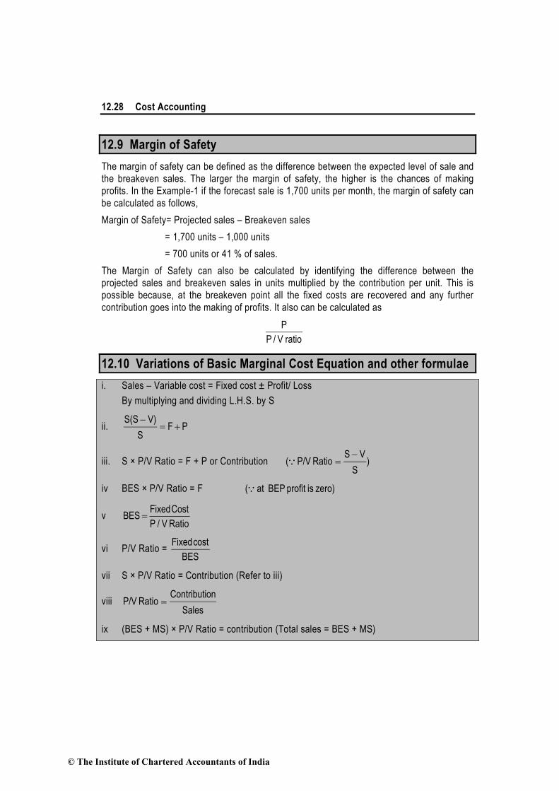
12.28 Cost Accounting
12.9 Margin of Safety
The margin of safety can be defined as the difference between the expected level of sale and the breakeven sales. The larger the margin of safety, the higher is the chances of making profits. In the Example-1 if the forecast sale is 1,700 units per month, the margin of safety can be calculated as follows, Margin of Safety= Projected sales – Breakeven sales = 1,700 units – 1,000 units = 700 units or 41 % of sales. The Margin of Safety can also be calculated by identifying the difference between the projected sales and breakeven sales in units multiplied by the contribution per unit. This is possible because, at the breakeven point all the fixed costs are recovered and any further contribution goes into the making of profits. It also can be calculated as
ratioV/PP
12.10 Variations of Basic Marginal Cost Equation and other formulae
i. Sales – Variable cost = Fixed cost ± Profit/ Loss By multiplying and dividing L.H.S. by S
ii. PFS
V)S(S+=
−
iii. S × P/V Ratio = F + P or Contribution )S
VSRatioP/V ( −=
iv BES × P/V Ratio = F zero) isprofit BEPat (
v FixedCostBES P / V Ratio
=
vi P/V Ratio = FixedcostBES
vii S × P/V Ratio = Contribution (Refer to iii)
viii Sales
onContributiRatioP/V =
ix (BES + MS) × P/V Ratio = contribution (Total sales = BES + MS)
© The Institute of Chartered Accountants of India

Marginal Costing 12.29
x (BES × P/V Ratio) + (MS × P/V Ratio) = F + P
By deducting (BES × P/V Ratio) from L.H.S. and F from R.H.S. in x we get :
xi M.S. × P/V Ratio = P
xii P/V Ratio = sales in Changeprofit in Change
xiii P/V Ratio = sales in Change
oncontributi in Change
xiv Profitability = factorKey
onContributi
xv Margin of Safety = Total Sales – BES or ratioV/PofitPr
.
xvi BES = Total Sales – MS
Margin of Safety Ratio = sales Total
BES - sales Total
Illustration 14 (Application of marginal cost equation) An automobile manufacturing company produces different models of Cars. The budget in
respect of model 007 for the month of March, 2015 is as under:
Budgeted Output 40,000 Units
` In lakhs ` In lacs
Net Realisation 700
Variable Costs:
Materials 264
Labour 52
Direct expenses 124 440
Specific Fixed Costs 90
Allocated Fixed Costs 112.50 202.50
Total Costs 642.50
Profit 57.50
Sales 700.00
© The Institute of Chartered Accountants of India

12.30 Cost Accounting
Calculate:
(i) Profit with 10 percent increase in selling price with a 10 percent reduction in sales
volume.
(ii) Volume to be achieved to maintain the original profit after a 10 percent rise in material
costs, at the originally budgeted selling price per unit.
Solution:
(i) Budgeted selling price = 700 lakhs/ 40,000 units = ` 1,750 per unit. Budgeted variable cost = 440 lakhs/ 40,000 units = ` 1,100 per unit. Increased selling price = 1,750 + 10% = ` 1,925 per unit New volume 40,000 – 10% = 36,000 units
Statement of Calculation of Profit:
(` In lakhs) Sales 36,000 units at ` 1,925 = 693.00 Less: Variable cost: 36,000 × 1,100 = 396.00 Contribution 297.00 Less: fixed costs 202.50 Profit 94.50
(ii) Budgeted Material cost = 264 lakhs/ 40,000 units = ` 660 per unit Increased material cost = 660×110% = 726 Labour cost 52 lakhs/ 40,000 units = 130 Direct expenses, 124 lakhs/ 40,000 units = 310 Variable cost per unit 1,166 Budgeted selling price per unit 1,750 Contribution per unit(1,750 – 1,166) 584
Sales volume = Fixedcos ts Pr ofit 202.50 lakhs + 57.50 lakhsContribution Per Unit 584
+=
`
= 44,521 units are to be sold to maintain the original profit of ` 57.50 lakhs. Illustration 15 (Calculation of margin of safety)
A company earned a profit of ` 30,000 during the year 2014. If the marginal cost and selling
price of the product are ` 8 and ` 10 per unit respectively, find out the amount of margin of
safety.
© The Institute of Chartered Accountants of India

Marginal Costing 12.31
Solution:
P/V ratio = S
VS − = 10
810 − = 20%
Margin of safety = ratioP/V
Profit = 20%
30,000 = ` 1,50,000
Illustration 16 (Calculation of margin of safety)
A Ltd. Maintains margin of safety of 37.5% with an overall contribution to sales ratio of 40%.
Its fixed costs amount to ` 5 lakhs.
Calculate the following:
i. Break-even sales
ii. Total sales
iii. Total variable cost
iv. Current profit
v. New ‘margin of safety’ if the sales volume is increased by 7 ½ %.
Solution:
(i) We know that: Break Even Sales (BES) x P/V Ratio = Fixed Cost Break Even Sales (BES) x 40% = ` 5,00,000 Break Even Sales (BES) = ` 12,50,000
(ii) Total Sales = Break Even Sales + Margin of Safety S = ` 12,50,000 + 0.375S
S – 0.375S = ` 12,50,000 S = ` 20,00,000 (iii) Contribution to Sales Ratio = 40% Therefore, Variable cost to Sales Ratio = 60% Variable cost = 60% of sales
= 60% of 20,00,000 Variable cost = 12,00,000 (iv) Current Profit = Sales – (Variable Cost + Fixed Cost)
= ` 20,00,000 – (12,00,000 + 5,00,000) = ` 3,00,000 (v) If sales value is increased by 7 ½ % New Sales value = ` 20,00,000 x 1.075 = ` 21,50,000
© The Institute of Chartered Accountants of India

12.32 Cost Accounting
New Margin of Safety = New Sales value – BES = ` 21,50,000 – ` 12,50,000 = ` 9,00,000 Illustration 17 (Calculation of margin of safety)
You are given the following data :
Sales Profit
Year 2013 ` 1,20,000 8,000
Year 2014 ` 1,40,000 13,000
Find out –
(i) P/V ratio,
(ii) B.E. Point,
(iii) Profit when sales are `1,80,000,
(iv) Sales required earn a profit of `12,000,
(v) Margin of safety in year 2014.
Solution:
Sales Profit
Year 2013 ` 1,20,000 8,000 Year 2014 ` 1,40,000 13,000 Difference ` 20,000 5,000
(i) P/V Ratio = SalesinDifferenceprofitin Difference ×100 =
20,0005,000 × 100 = 25 %
(`) Contribution in 2013 (1,20,000 × 25%) 30,000
Less : Profit 8,000 Fixed Cost* 22,000
*Contribution = Fixed cost + Profit ∴ Fixed cost = Contribution - Profit
(ii) Break-even point = ratioP/VcostFixed =
25%22,000 = ` 88,000
(iii) Profit when sales are `1,80,000 (`) Contribution (`1,80,000 × 25%) 45,000
© The Institute of Chartered Accountants of India

Marginal Costing 12.33
Less: Fixed cost 22,000 Profit 23,000
(iv) Sales to earn a profit of `12,000
ratioP/VprofitDesiredcostFixed + =
25%12,00022,000 + = `1,36,000
(v) Margin of safety in 2014 – Margin of safety = Actual sales – Break-even sales
= 1,40,000 – 88,000 = ` 52,000. Illustration 18 (Calculation of selling price)
A single product company sells its product at ` 60 per unit. In 2013, the company operated at
a margin of safety of 40%. The fixed costs amounted to ` 3,60,000 and the variable cost ratio
to sales was 80%.
In 2014, it is estimated that the variable cost will go up by 10% and the fixed cost will increase
by 5%.
(i) Find the selling price required to be fixed in 2014 to earn the same P/V ratio as in 2013.
(ii) Assuming the same selling price of ` 60 per unit in 2014, find the number of units
required to be produced and sold to earn the same profit as in 2013.
Solution:
(i) Profit earned in 2013:
(`)
Total contribution (50,000 × ` 12) 6,00,000
Less: Fixed cost 3,60,000 2,40,000 Selling price to be fixed in 2014:
Revised variable cost (` 48 × 1.10) 52.80
Revised fixed cost (3,60,000 × 1.05) 3,78,000
P/V Ratio (Same as of 2013) 20% Variable cost ratio to selling price 80%
Therefore revised selling price per unit = ` 52.80 ÷ 80% = ` 66
© The Institute of Chartered Accountants of India

12.34 Cost Accounting
(ii) No. of units to be produced and sold in 2014 to earn the same profit:
We know that Fixed Cost plus profit = Contribution (`) Profit in 2013 2,40,000 Fixed cost in 2014 3,78,000 Desired contribution in 2014 6,18,000
Contribution per unit = Selling price per unit – Variable cost per unit. = ` 60 – ` 52.80 = ` 7.20.
No. of units to be produced in 2014 = ` 6,18,000 ÷ ` 7.20 = 85,834 units. Workings:
1. PV Ratio in 2013 (`) Selling price per unit 60 Variable cost (80% of Selling Price) 48 Contribution 12 P/V Ratio 20%
2. No. of units sold in 2013 Break-even point = Fixed cost ÷ Contribution per unit
= ` 3,60,000 ÷ ` 12 = 30,000 units. Margin of safety is 40%. Therefore, break-even sales will be 60% of units sold. No. of units sold = Break-even point in units ÷ 60%
= 30,000 ÷ 60% = 50,000 units. Illustration 19 (Calculation of margin of safety)
A company has made a profit of ` 50,000 during the year 2013-14. If the selling price and marginal cost of the product are ` 15 and ` 12 per unit respectively, find out the amount of margin of safety.
Solution:
P/V Ratio = ContributionSales
x 100
= [(15 – 12)/15] x 100 = (3/15) x 100 = 20%
© The Institute of Chartered Accountants of India

Marginal Costing 12.35
Marginal of Safety = (Profit)/ (P/V Ratio) = 50,000/20% = ` 2,50,000 Illustration 20 (Calculation of break even sales)
(a) If margin of safety is ` 2,40,000 (40% of sales) and P/V ratio is 30% of AB Ltd, calculate
its (1) Break even sales, and (2) Amount of profit on sales of `9,00,000.
(b) X Ltd. has earned a contribution of `2,00,000 and net profit of `1,50,000 of sales of ` 8,00,000. What is its margin of safety?
Solution:
(a) Total Sales = 2,40,000 × 10040
= `6,00,000
Contribution = 6,00,000 × 30% = `1,80,000 Profit = M/S × P/V ratio = 2,40,000 × 30% = `72,000 Fixed cost = Contribution – Profit = 1,80,000 – 72,000 = `1,08,000
(1) Break-even Sales = tFixed CostP/V ratio
= 30%
1,08,000 = `3,60,000
(2) Profit = (Sales × P/V ratio) – Fixed cost = (9,00,000 × 30%) – 1,08,000 = `1,62,000
(b) P/V ratio = ContributionSales
= 8,00,0002,00,000 = 25%
Margin of safety = ratioP/V
Profit = 25%
1,50,000 = ` 6,00,000
Alternatively : Fixed cost = Contribution – Profit =` 2,00,000 – `1,50,000 = ` 50,000 B.E. Point = ` 50,000 ÷ 25% = ` 2,00,000 Margin of Safety = Actual sales – B.E. sales = 8,00,000 – 2,00,000 = 6,00,000 Illustration 21 (Calculation of break even sales and margin of safety)
A company had incurred fixed expenses of ` 4,50,000, with sales of ` 15,00,000 and earned
a profit of ` 3,00,000 during the first half year. In the second half, it suffered a loss of
© The Institute of Chartered Accountants of India

12.36 Cost Accounting
` 1,50,000.
Calculate:
(i) The profit-volume ratio, break-even point and margin of safety for the first half year.
(ii) Expected sales volume for the second half year assuming that selling price and fixed
expenses remained unchanged during the second half year.
(iii) The break-even point and margin of safety for the whole year.
Solution:
(i) In the First half year
Contribution = Fixed cost + Profit
= 4,50,000 + 3,00,000 = ` 7,50,000
P/V ratio = ContributionSales
x 100 = 15,00,0007,50,000 x 100 = 50%
Break-even point = ratioP/VcostFixed =
50%4,50,000 x 100 = ` 9,00,000
Margin of safety= Actual sales – Break-even point
= 15,00,000 – 9,00,000 = ` 6,00,000
(ii) In the second half year
Contribution = Fixed cost – Loss
= 4,50,000 – 1,50,000 = ` 3,00,000
Expected sales volume = ratioP/V
LosscostFixed − = 50%
3,00,000 = ` 6,00,000
(iii) For the whole year
B.E. point = ratioP/VcostFixed =
50%24,50,000× = `18,00,000
Margin of safety = ratioP/V
Profit = 50%
1,50,0003,00,000 − = ` 3,00,000.
Illustration 22 (Calculation of Break even Sales, Profit and Fixed Cost)
The following information is given by Star Ltd.:
Margin of Safety ` 1,87,500
© The Institute of Chartered Accountants of India

Marginal Costing 12.37
Total Cost ` 1,93,750
Margin of Safety 3,750 units
Break-even Sales 1,250 units
Required:
Calculate Profit, P/V Ratio, BEP Sales (in`) and Fixed Cost.
Solution:
Margin of Safety (%) = 3,750uni t s3,750units 1,250units+
= 75%
Total Sales = 1,87,5000.75
`
= `2,50,000
Profit = Total Sales – Total Cost
= `2,50,000 – `1,93,750
= `56,250
P/V Ratio = Pr ofit 100Marginof Safety ( )
×`
= ×56,250 100
1,87,500`
`
= 30%
Break-even Sales = Total Sales × [100 – Margin of Safety %]
= ` 2,50,000 × 0.25
= ` 62,500
Fixed Cost = Sales × P/V Ratio – Profit
= `2,50,000 × 0.30 – `56,250
= `18,750 Illustration 23 (Implication of changes in different variables on P/V ratio)
By noting “P/V will increase or P/V will decrease or P/V will not change”, as the case may be,
state how the following independent situations will affect the P/V ratio:
© The Institute of Chartered Accountants of India

12.38 Cost Accounting
(i) An increase in the physical sales volume;
(ii) An increase in the fixed cost;
(iii) A decrease in the variable cost per unit;
(iv) A decrease in the contribution margin;
(v) An increase in selling price per unit;
(vi) A decrease in the fixed cost;
(vii) A 10% increase in both selling price and variable cost per unit;
(viii) A 10% increase in the selling price per unit and 10% decrease in the physical sales
volume;
(ix) A 50% increase in the variable cost per unit and 50% decrease in the fixed cost.
(x) An increase in the angle of incidence.
Solution:
Item no. P/V Ratio Reason
(i) Will not change (ii) Will not change (iii) Will increase (iv) Will decrease (v) Will increase (vi) Will not change (vii) Will not change Reasoning 1 (viii) Will increase Reasoning 2 (ix) Will decrease Reasoning 3 (x) Will increase Reasoning 4
A 10%increase in both selling price and variable cost per unit. Reasoning 1. Assumptions: a) Variable cost is less than selling price. b) Selling price `100 variable cost ` 90 per unit.
c) P/V ratio = 100 90100− = 10%
10% increase in S.P. = `110 10% increase in variable cost = `99
© The Institute of Chartered Accountants of India

Marginal Costing 12.39
P/V ratio = 110 9910− = 10% i.e. P/v ratio will not change
Reasoning 2. Increase or decrease in physical sales volume will not change P/v ratio. Hence 10% increase in selling price per unit will increase P/V ratio.
Reasoning 3. Increase or decrease in fixed cost will not change P/V ratio. Hence 50% increase in the variable cost per unit will decrease P/V ratio.
Reasoning 4. Angle of incidence is the angle at which sales line cuts the total cost line. If it is large, it indicates that the profits are being made at higher rate. Hence increase in the angle of incidence will increase the P/V ratio.
12.11 Angle of Incidence
This angle is formed by the intersection of sales line and total cost line at the break-even point. This angle shows the rate at which profits are being earned once the break-even point has been reached. The wider the angle the greater is the rate of earning profits. A large angle of incidence with a high margin of safety indicates extremely favourable position. The shaded area in the graph given below is representing the angle of incidence. The angle above and below the break-even point shows the rate of earning profitability (loss). Wider angle denotes higher rate of earnings and vice-versa.
280
260
240
220
200
180
160
140
120
100
80
60
40
20
0
2 4 6 8 10 12 14 16 18 20 22 24 26 28
Fixed cost
Variable cost
Break even point
Co
st a
nd
Sa
les
(Rs.
‘ 0
00
)
Margin of
Safety
Margin of
Safety
Total Cost Line
Loss Are
a
Pro
fit A
rea
Sales L
ine
Angle ofincidence
Volume of sales (Unit ‘000)
B.E.sales Actual sales
© The Institute of Chartered Accountants of India

12.40 Cost Accounting
12.12 Graphical Representation of Break Even Chart
12.12.1 Break-even Chart : A breakeven chart records costs and revenues on the vertical axis and the level of activity on the horizontal axis. The making of the breakeven chart would require you to select appropriate axes. Subsequently, you will need to mark costs/revenues on the Y axis whereas the level of activity shall be traced on the X axis. Lines representing (i) Fixed costs (horizontal line at ` 2,00,000 for ABC Ltd), (ii) Total costs at maximum level of activity (joined to the Y-axis where the Fixed cost of ` 2,00,000 is marked) and (iii) Revenue at maximum level of activity (joined to the origin) shall be drawn next. The breakeven point is that point where the sales revenue line intersects the total cost line. Other measures like the margin of safety and profit can also be measured from the chart. The breakeven chart for ABC Ltd (Example-1) is drawn below.
12.12.2 Contribution Breakeven chart: It is not possible to use a breakeven chart as described above to measure contribution. This is one of its major limitations especially so because contribution analysis is literally the backbone of marginal costing. To overcome such a limitation, accountants frequently resort to the making of a contribution breakeven chart which is based on the same principles as a conventional breakeven chart except for that it shows the variable cost line instead of the fixed cost line. Lines for Total cost and Sales revenue remain the same. The breakeven point and profit can be read off in the same way as with a conventional chart. However it is also possible to read the contribution for any level of activity. Using the same example of ABC Ltd as for the conventional chart, the total variable cost for an output of 1,700 units is 1,700 × `300 = `5,10,000. This point can be joined to the origin since the variable cost is nil at zero activity.
© The Institute of Chartered Accountants of India

Marginal Costing 12.41
The contribution can be read as the difference between the sales revenue line and the variable cost line. 12.12.3 Profit-volume chart: This is also very similar to a breakeven chart. In this chart the vertical axis represents profits and losses and the horizontal axis is drawn at zero profit or loss. In this chart each level of activity is taken into account and profits marked accordingly. The breakeven point is where this line interacts the horizontal axis. A profit-volume graph for our example (ABC Ltd) will be as follows,
Loss
The loss at a nil activity level is equal to ` 2,00,000, i.e. the amount of fixed costs. The second point used to draw the line could be the calculated breakeven point or the calculated profit for sales of 1,700 units.
© The Institute of Chartered Accountants of India

12.42 Cost Accounting
Advantages of the profit-volume chart
1. The biggest advantage of the profit-volume chart is its capability of depicting clearly the effect on profit and breakeven point of any changes in the variables. The following example illustrates this characteristic,
Example 2:
A manufacturing company incurs fixed costs of `3,00,000 per annum. It is a single product company with annual sales budgeted to be 70,000 units at a sales price of `300 per unit. Variable costs are `285 per unit. (i) Draw a profit volume graph, and use it to determine the breakeven point. The company is deliberating upon an increase in the selling price of the product to `350
per unit. This shall be required in order to improve the quality of the product. It is anticipated that despite increase in the selling price the sales volume shall remain unaffected, however, the fixed costs shall increase to `4,50,000 per annum and the variable costs to `330 per unit.
(ii) Draw on the same graph as for part (a) a second profit volume graph and give your comments.
Solution:
Figure showing changes with a profit-volume chart
© The Institute of Chartered Accountants of India
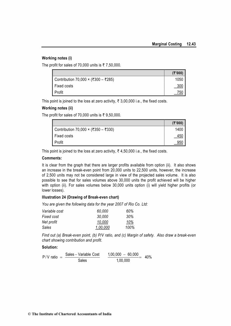
Marginal Costing 12.43
Working notes (i)
The profit for sales of 70,000 units is ` 7,50,000.
(`’000)
Contribution 70,000 × (`300 – `285) 1050 Fixed costs 300 Profit 750
This point is joined to the loss at zero activity, ` 3,00,000 i.e., the fixed costs. Working notes (ii)
The profit for sales of 70,000 units is ` 9,50,000.
(`’000)
Contribution 70,000 × (`350 – `330) 1400 Fixed costs 450 Profit 950
This point is joined to the loss at zero activity, ` 4,50,000 i.e., the fixed costs. Comments:
It is clear from the graph that there are larger profits available from option (ii). It also shows an increase in the break-even point from 20,000 units to 22,500 units, however, the increase of 2,500 units may not be considered large in view of the projected sales volume. It is also possible to see that for sales volumes above 30,000 units the profit achieved will be higher with option (ii). For sales volumes below 30,000 units option (i) will yield higher profits (or lower losses). Illustration 24 (Drawing of Break-even chart)
You are given the following data for the year 2007 of Rio Co. Ltd:
Variable cost 60,000 60%
Fixed cost 30,000 30%
Net profit 10,000 10%
Sales 1,00,000 100%
Find out (a) Break-even point, (b) P/V ratio, and (c) Margin of safety. Also draw a break-even
chart showing contribution and profit.
Solution:
Sales Variable Cost 1,00,000 60,000P / V ratio 40%Sales 1,00,000
− −= = =
© The Institute of Chartered Accountants of India

12.44 Cost Accounting
Rs`
Fixed Cost 30,000Break Even Po int 75,000P/V ratio 40%
= = =
Margin of safety = Actual Sales – BE point = 1,00,000 – 75,000 = ` 25,000 Break even chart showing contribution is shown below:
Break-even chart
Illustration 25 (Drawing of Break-even chart)
(a) You are given the following data for the coming year for a factory.
Budgeted output 8,00,000 units
Fixed expenses 40,00,000
Variable expenses per unit ` 100
Selling price per unit ` 200
Draw a break-even chart showing the break-even point.
(b) If price is reduced to ` 180, what will be the new break-even point?
© The Institute of Chartered Accountants of India

Marginal Costing 12.45
Solution:
(a) Contribution = S – V = ` 200 – ` 100 = ` 100 per unit.
units
R`
Fixed cos t 40,00,000B.E. Po int 40,000Contribution per unit 100
= = =
(b) When selling price is reduced New selling price = ` 180 New Contribution = ` 180 – ` 100 = ` 80 per unit.
New `
`
40,00,000B.E. Po int 50,000 units.80
= =
The break-even chart is shown below:
0
200
160
120
80
40
Cost and R
evenue (
Rs.'00000)
20 40 60 80 10050
Fixed cost line
New break-even point
New sale
s lin
e
Sales
line
B.E.P.
Output ('000 units)
Total cost line
Illustration 26 (Drawing of Profit Graph)
Prepare a profit graph for products A, B and C and find break-even point from the following
data:
© The Institute of Chartered Accountants of India

12.46 Cost Accounting
Products A B C Total
Sales (`) 7,500 7,500 3,750 18,750
Variable cost (`) 1,500 5,250 4,500 11,250
Fixed cost (`) --- --- --- 5,000
Solution:
Statement Showing Cumulative Sales & Profit
Sales Cumulative Sales Variable Cost
Contribution Cumulative Contribution
Cumulative Profit
(`) (`) (`) (`) (`) (`)
A 7,500 7,500 1,500 6,000 6,000 1,000 B 7,500 15,000 5,250 2,250 8,250 3,250 C 3,750 18,750 4,500 (750) 7,500 2,500
Profit in `
(+) 5,000
`3,250 (+) 2,500 `2,500 `1,000
0 2,500 5,000 7,500 10,000 12,500 15,000 17,500 20,000
BEP Sales in `
(-) 2,500 Profit Line
(-) 5,000
Loss in `
Break Even Point (BEP) = ` 12,500
12.13 The Limitations of Breakeven Analysis
The limitations of the practical applicability of breakeven analysis and breakeven charts stem mostly from the assumptions underlying CVP which have been mentioned above. Assumptions like costs behaving in a linear fashion or sales revenue remain constant at different sales levels or the stocks shall remain constant period after period are unrealistic. Similarly, the assumption that the only factor which influences costs is the ‘activity level achieved’ is erroneous because other factors like inflation also have a bearing on costs.
© The Institute of Chartered Accountants of India

Marginal Costing 12.47
12.14 Summary
• Absorption Costing: a method of costing by which all direct cost and applicable overheads are charged to products or cost centers for finding out the total cost of production. Absorbed cost includes production cost as well as administrative and other cost.
• Break-even Chart: A mathematical or graphical representation, showing approximate profit or loss of an enterprise at different levels of activity within a limited range.
• Break-even Point the level of activity there is neither a profit nor a loss.
Break-even Point in units =Fixed costs
Contribution per unit
• Cash Break Even Point the level of activity where there is neither a cash profit nor a cash loss.
• Cost Breakeven Point the level of activity where the total cost under two alternatives are the same. It is also known as Cost indifference point.
• Differential Costing a technique used in the preparation of adhoc information in which only cost and income differences in between alternative courses of action are taken into consideration.
• Direct Costing a principle under which all costs which are directed related are charged to products, processes, operations or services, of which they form an integral part.
• Marginal Contribution difference between selling price and variable cost of production. • Marginal Cost the variable cost of one unit of product or a service.
• Marginal Cost Equation : S × U – V × U = F ± P
• Marginal Costing a principle whereby variable cost are charged to cost units and fixed cost attributable to the relevant period is written off in full against contribution for that period.
• Profit Volume Chart a diagram showing the expected relationship between costs, revenue at various volumes with profit being the residual.
• Profit Volume Ratio the ratio establishing the relationship between the contribution and the sales value.
• Margin of Safety is the difference between the expected level of sales and the break even sales
• Projected Sales – Break even sales
© The Institute of Chartered Accountants of India

13
Budgets and Budgetary Control
Learning Objectives
When you have finished studying this chapter, you should be able to
Understand the objectives and importance of budgeting and budgetary control
Understand the Advantages and disadvantages of budgetary control
Differentiate between various types of budgets.
Understand the process of preparation of budgets
13.1 Introduction
Budgetary control and standard costing systems are two essential tools frequently used by
business executives for the purpose of planning and control. In the case of budgetary control,
the entire exercise starts with the setting up of budgets or targets and ends with the taking of
an action, in case the actual figures differed with the budgetary ones.
13.2 Meaning of Budget and Budgeting
Budget: CIMA Official Terminology has defined the terms ‘budget’ as “Quantitative expression of a
plan for a defined period of time. It may include planned sales volumes and revenues; resource
quantities, costs and expenses; assets, liabilities and cash flows.”
Budgeting: It is a means of coordinating the combined intelligence of an entire organisation
into a plan of action based on past performance and governed by rational judgment of factors
that will influence the course of business in the future.
13.3 Essentials of Budget
Essential elements of a budget are as follows:
1. Organisational structure must be clearly defined and responsibility should be assigned
to identifiable units within the organisation.
2. Setting of clear objectives and reasonable targets. Objectives should be in consonance
with the long term plan of the organisation.
© The Institute of Chartered Accountants of India

Budgets and Budgetary Control 13.2
3. Objectives and degree of responsibility should be clearly stated and communicated to
the management or person responsible for.
4. Budgets are prepared for the future periods based on expected course of actions.
5. Budgets are updated for the events that were not kept into the mind while establishing
budgets. Hence, budgets should flexible enough for mid- term revision.
6. The entire organisation must be committed to budgeting.
7. Budgets should be quantifiable and master budget should be broken down into various
functional budgets.
8. Budgets should be monitored periodically. Variances from the set yardsticks (standards)
should be analysed and responsibility should be fixed.
9. Budgetary performance needs to be linked effectively to the reward system.
13.4 Characteristic of Budget
The main characteristics of budget are as follows:
1. A budget is concerned for a definite future period.
2. A budget is a written document.
3. A budget is a detailed plan of all the economic activities of a business.
4. All the departments of a business unit co-operate for the preparation of a business
budget.
5. Budget is a mean to achieve business and it is not an end in itself.
6. Budget needs to be updated, corrected and controlled every time when circumstances
changes. Therefore it is a continuous process.
7. Budget helps in planning, coordination and control.
8. Different types of budgets are prepared by industries according to business requirements.
9. A budget acts a business barometer.
10. Budget is usually prepared in the light of Past Experience.
11. Budget is a constant endeavour of the Management.
13.5 Objectives of Budgeting
Planning:
The process of budgeting begin with the establishment of specific targets of performance and
is followed by executing plans to achieve such desired goals and from time to time comparing
actual results with the target goals. These targets include both the overall business targets as
well as the specific targets for the individual units within the business. Establishing specific
© The Institute of Chartered Accountants of India

13.3 Cost Accounting
targets for future operations is part of the planning function of management, while executing
actions to meet the goals is the directing function of management. It may be explained as
Budgets plans are made taking into account the objectives at different level of an organization i.e. Mission, corporate strategy and unit objectives. Individual plans at unit level should take overall organizational plan or objectives.
Budgets reflect plans and that planning should have taken place before budgets are prepared.
Budgets plans are quantified and responsibility is assigned to the persons who are responsible for execution of plan.
Using the budget to communicate these expectations throughout the organization has helped many a companies to reduce expenses during a severe business recession.
Planning not only motivates employees to attain goals but also improves overall decision making. During the planning phase of the budget process, all viewpoints are considered, options identified, and cost reduction opportunities assessed. This process may reveal opportunities or threats that were not known prior to the budget planning process.
Directing and Coordinating:
Once the budget plans are in place, they can be used to direct and coordinate operations in order to achieve the stated targets.
A business, however, is much more complex and requires more formal direction and coordination.
The budget is one way to direct and coordinate business activities and units to achieve stated targets of performance.
The budgetary units of an organisation are called responsibility centers. Each responsibility center is led by a manager who has the authority over and responsibility for the unit’s performance.
Objectives and degree of performance expected from a responsibility centres are communicated rapidly.
Controlling:
As time passes, the actual performance of an operation can be compared against the planned targets. This provides prompt feedback to employees about their performance. If necessary, employees can use such feedback to adjust their activities in the future.
Feedback received in the form of budget report from the responsibility centre. This report is helpful to know the performance of the concerned unit.
Any unexpected changes into the conditions which were prevailing at the time of preparing budget are taken into account and budgets are revised to show true performance yardstick.
Comparing actual results to the plan also helps prevent unplanned expenditures. The budget encourages employees to establish their spending priorities.
The main objective of Budgeting is to help in achieving the overall objective of the organization.
© The Institute of Chartered Accountants of India

Budgets and Budgetary Control 13.4
13.6 Meaning of Budgetary Control
CIMA has defined the terms ‘budgetary control’ as “Budgetary control is the establishment of
budgets relating to the responsibilities of executives of a policy and the continuous comparison
of the actual with the budgeted results, either to secure by individual action the objective of the
policy or to provide a basis for its revision.” It is the system of management control and
accounting in which all the operations are forecasted and planned in advance to the extent
possible and the actual results compared with the forecasted and planned ones.
13.6.1 Budgetary Control Involves:
1. Establishment of budgets
2. Continuous comparison of actual with budgets for achievement of targets
3. Revision of budgets after considering changed circumstances
4. Placing the responsibility for failure to achieve the budget targets.
13.6.2 The salient features of such a system are the following :
1. Determining the objectives to be achieved, over the budget period, and the policy or
policies that might be adopted for the achievement of these ends.
2. Determining the variety of activities that should be undertaken for the achievement of the
objectives.
3. Drawing up a plan or a scheme of operation in respect of each class of activity, in physical
as well as monetary terms for the full budget period and its parts.
4. Laying out a system of comparison of actual performance by each person, section or department
with the relevant budget and determination of causes for the discrepancies, if any.
5. Ensuring that corrective action will be taken where the plan is not being achieved and, if
that be not possible, for the revision of the plan.
In brief, it is a system to assist management in the allocation of responsibility and authority, to
provide it with aid for making, estimating and planning for the future and to facilitate the analysis
of the variation between estimated and actual performance.
In order that budgetary control may function effectively, it is necessary that the concern should
develop proper basis of measurement or standards with which to evaluate the efficiency of
operations, i.e., it should have in operation a system of standard costing.
Beside this, the organisation of the concern should be so integrated that all lines of authority
and responsibility are laid, allocated and defined. This is essential since the system of budgetary
control postulates separation of functions and division of responsibilities and thus requires that
the organisation shall be planned in such a manner that everyone, from the Managing Director
down to the Shop Foreman, will have his duties properly defined.
© The Institute of Chartered Accountants of India

13.5 Cost Accounting
13.6.3 Objectives of Budgetary Control System:
1. Portraying with precision the overall aims of the business and determining targets of
performance for each section or department of the business.
2. Laying down the responsibilities of each of the executives and other personnel so that
everyone knows what is expected of him and how he will be judged. Budgetary control is
one of the few ways in which an objective assessment of executives or department is
possible.
3. Providing a basis for the comparison of actual performance with the predetermined targets
and investigation of deviation, if any, of actual performance and expenses from the
budgeted figures. This naturally helps in adopting corrective measures.
4. Ensuring the best use of all available resources to maximise profit or production, subject
to the limiting factors. Since budgets cannot be properly drawn up without considering all
aspects usually there is good co-ordination when a system of budgetary control operates.
5. Co-ordinating the various activities of the business, and centralising control and yet
enabling management to decentralise responsibility and delegate authority in the overall
interest of the business.
6. Engendering a spirit of careful forethought, assessment of what is possible and an attempt
at it. It leads to dynamism without recklessness. Of course, much depends on the
objectives of the firm and the vigour of its management.
7. Providing a basis for revision of current and future policies.
8. Drawing up long range plans with a fair measure of accuracy.
9. Providing a yardstick against which actual results can be compared.
13.6.4 Working of a budgetary control system:
The responsibility for successfully introducing and implementing a Budgetary Control System
rests with the Budget Committee acting through the Budget Officer. The Budget Committee
would be composed of all functional heads and a member from the Board to preside over and
guide the deliberations.
The main responsibilities of the Budget Officer are:
1. to assist in the preparation of the various budgets by coordinating the work of the accounts
department which is normally responsible to compile the budgets—with the relevant func-
tional departments like Sales, Production, Plant maintenance etc.;
2. to forward the budget to the individuals who are responsible to adhere to them, and to
guide them in overcoming any practical difficulties in its working;
3. to prepare the periodical budget reports for circulation to the individuals concerned;
4. to follow-up action to be taken on the budget reports;
© The Institute of Chartered Accountants of India

Budgets and Budgetary Control 13.6
5. to prepare an overall budget working report for discussion at the Budget Committee
meetings and to ensure follow-up on the lines of action suggested by the Committee;
6. to prepare periodical reports for the Board meeting. Comparing the budgeted Profit and
Loss Account and the Balance Sheet with the actual results attained.
It is necessary that every budget should be thoroughly discussed with the functional head before
it is finalised.
It is the duty of the Budget Officer to see that the periodical budget reports are supplied to the
recipients at frequent intervals as far as possible.
The efficiency of the Budget Officer, and through him of the Budget Committee, will be judged
more by the smooth working of the system and the agreement between the actual figures and
the budgeted figures.
Budgets are primarily an incentive and a challenge for better performance; it is up to the Budget
Officer to see that attention of the different functional heads is drawn to it to face the challenge
in a successful manner.
13.6.5 Advantages of Budgetary Control System:
Points Description
1. Efficiency The use of budgetary control system enables the management of a business concern to conduct its business activities in the efficient manner.
2. Control on expenditure It is a powerful instrument used by business houses for the control of their expenditure. It in fact provides a yardstick for measuring and evaluating the performance of individuals and their departments.
3. Finding deviations It reveals the deviations to management, from the budgeted figures after making a comparison with actual figures.
4. Effective utilisation of resources
Effective utilisation of various resources like—men, material, machinery and money—is made possible, as the production is planned after taking them into account.
5. Revision of plans It helps in the review of current trends and framing of future policies.
6. Implementation of Standard Costing system
It creates suitable conditions for the implementation of standard costing system in a business organisation.
7. Cost Consciousness Budgets are studied by outside fund providers also such as banking and financial institutions, realising that management encourages cost consciousness and maximum utilisation of available resources.
© The Institute of Chartered Accountants of India

13.7 Cost Accounting
8. Credit Rating Management which have developed a well ordered budget plans and which operate accordingly, receive greater favour from credit agencies.
13.6.6 Limitations of Budgetary Control System:
Points Description
1. Based on Estimates Budgets are based on series of estimates which are based on
the conditions prevailed or expected at the time budget is
established. It requires revision in plan if conditions change.
2. Time factor Budgets cannot be executed automatically. Some preliminary
steps are required to be accomplished before budgets are
implemented. It requires proper attention and time of
management. Management must not expect too much during
the development period.
3. Co-operation Required
Staff co-operation is usually not available during budgetary
control exercise. In a decentralised organisation each unit has
its own objective and these units enjoy some degree of
discretion. In this type of organisation structure coordination
among different units are required. The success of the
budgetary control depends upon willing co-operation and
teamwork,
4. Expensive Its implementation is quite expensive. For successful
implementation of the budgetary control proper organisation
structure with responsibility is prerequisite. Budgeting process
start from the collection of requirements to budget and
performance analysis. It consumes valuable resources for
these purpose, hence, it is an expensive process.
5. Not a substitute for management
Budget is only a managerial tool and must be applied correctly
for management to get benefited. Budgets are not a substitute
for management.
6. Rigid document Budgets are considered as rigid document. But in reality, an
organisation is exposed to various uncertain internal and
external factors. Budget should be flexible enough to
incorporate ongoing developments in the internal and external
factors affecting the very purpose of the budget.
© The Institute of Chartered Accountants of India

Budgets and Budgetary Control 13.8
13.6.7 Components of Budgetary Control System:
The policy of a business for a defined period is represented by the master budget the details of
which are given in a number of individual budgets called functional budgets. These functional
budgets are broadly grouped under the following heads:
1. Physical budgets: Those budgets which contain information in terms of physical units about
sales, production etc. for example, quantity of sales, quantity of production, inventories,
and manpower budgets are physical budgets.
2. Cost budgets: Budgets which provides cost information in respect of manufacturing,
selling, administration etc. for example, manufacturing costs, selling costs, administration
cost, and research and development cost budgets are cost budgets.
3. Profit budgets: A budget which enables in the ascertainment of profit, for example, sales
budget, profit and loss budget, etc.
4. Financial budgets: A budget which facilitates in ascertaining the financial position of a
concern, for example, cash budgets, capital expenditure budget, budgeted balance sheet
etc.
13.7 Preparation of Budgets
1. Definition of objectives: A budget being a plan for the achievement of certain operational
objectives, it is desirable that the same are defined precisely. The objectives should be
written out; the areas of control demarcated; and items of revenue and expenditure to be
covered by the budget stated. This will give a clear understanding of the plan and its scope
to all those who must cooperate to make it a success.
2. Location of the key (or budget) factor: There is usually one factor (sometimes there may
be more than one) which sets a limit to the total activity. For instance, in India today
sometimes non-availability of power does not allow production to increase inspite of heavy
demand. Similarly, lack of demand may limit production. Such a factor is known as key
factor. For proper budgeting, it must be located and estimated properly.
3. Appointment of controller: Formulation of a budget usually required whole time services
of a senior executive; he must be assisted in this work by a Budget Committee, consisting
of all the heads of department along with the Managing Director as the Chairman. The
Controller is responsible for coordinating and development of budget programmes and
preparing the manual of instruction, known as Budget manual.
4. Budget Manual: Effective budgetary planning relies on the provision of adequate
information to the individuals involved in the planning process. Many of these information
needs are contained in the budget manual. A budget manual is a collection of documents
© The Institute of Chartered Accountants of India

13.9 Cost Accounting
that contains key information for those involved in the planning process. Typical contents
could include the following:
An introductory explanation of the budgetary planning and control process, including
a statement of the budgetary objective and desired results.
A form of organisation chart to show who is responsible for the preparation of each
functional budget and the way in which the budgets are interrelated.
A timetable for the preparation of each budget. This will prevent the formation of a
‘bottleneck’ with the late preparation of one budget holding up the preparation of all
others.
Copies of all forms to be completed by those responsible for preparing budgets, with
explanations concerning their completion.
A list of the organization’s account codes, with full explanations of how to use them.
Information concerning key assumptions to be made by managers in their budgets,
for example the rate of inflation, key exchange rates, etc.
5. Budget period: The period covered by a budget is known as budget period. There is no
general rule governing the selection of the budget period. In practice the Budget
Committee determines the length of the budget period suitable for the business. Normally,
a calendar year or a period co-terminus with the financial year is adopted. The budget
period is then sub-divided into shorter periods; it may be months or quarters or such
periods as coincide with period of trading activity.
6. Standard of activity or output: For preparing budgets for the future, past statistics cannot
be completely relied upon, for the past usually represents a combination of good and bad
factors. Therefore, though results of the past should be studied but these should only be
applied when there is a likelihood of similar conditions repeating in the future. Also, while
setting the targets for the future, it must be remembered that in a progressive business,
the achievement of a year must exceed those of earlier years. Therefore what was good
in the past is only fair for the current year.
In budgeting, fixing the budget of sales and of capital expenditure is most important since these
budgets determine the extent of development activity. For budgeting sales, one must consider
the trend of economic activity of the country, reactions of salesmen, customers and employees,
effect of price changes on sales, the provision for advertisement campaign plan capacity etc.
© The Institute of Chartered Accountants of India

Budgets and Budgetary Control 13.10
13.8 Different Types of Budgets
BUDGET
Capacity wise Functional wise Master Budget Period wise
Sales budget
Fixed Flexible Production budget Long- term Short Current
Budgets Budgets Plant utilisation budget Budgets Budgets Budgets
Direct-material usage budget
Direct-material purchase budget
Direct-labour (personnel) budget
Factory overhead budget
Production cost budget
Ending-inventory budget
Cost of goods-sold budget
Selling and distribution cost budget
Administration expenses budget
Research and development cost budget
Capital expenditure budget
Cash budget
13.8.1 Classification on the basis of Capacity or Flexibility:
These types of budgets are prepared on the basis of activity level or utilization of capacity.
These are also known as “Budgets on the basis of flexibility”.
(i)
Fixed Budget : According to CIMA, “a fixed budget, is a budget designed to remain unchanged
irrespective of the level of activity actually attained”.
A fixed budget shows the expected results of a responsibility center for only one activity level.
Once the budget has been determined, it is not changed, even if the activity changes. Fixed
budgeting is used by many service companies and for some administrative functions of
manufacturing companies, such as purchasing, engineering, and accounting. Fixed Budget is
used as an effective tool of cost control. In case, the level of activity attained is different from
the level of activity for budgeting purposes, the fixed budget becomes ineffective. Such a budget
is quite suitable for fixed expenses. It is also known as a static budget.
© The Institute of Chartered Accountants of India

13.11 Cost Accounting
Essential conditions:
1. When the nature of business is not seasonal.
2. There is no impact of external factors on the business activities
3. The demand of the product is certain and stable.
4. Supply orders are issued regularly.
5. The market of the product should be domestic rather than foreign.
6. There is no need of special labour or material in the production of the products.
7. Supply of production inputs is regular.
8. There is a trend of price stability.
Generally, all above conditions are not found in practice. Hence Fixed budget is not important
in business concerns.
Merits and Demerits of fixed budgets are tabulated below:
Merits Demerits
1. Very simple to understand
2. Less time consuming
1. It is misleading. A poor performance
may remain undetected and a good
performance may go unrealised.
2. It is not suitable for long period.
3. It is also found unsuitable particularly
when the business conditions are
changing constantly.
4. Accurate estimates are not possible.
(ii) Flexible Budget: According to CIMA, “a flexible budget is defined as a budget which, by
recognizing the difference between fixed, semi-variable and variable costs is designed to
change in relation to the level of activity attained.” Unlike static (fixed) budgets, flexible budgets
show the expected results of a responsibility center for different activity levels.
You can think of a flexible budget as a series of static budgets for different levels of activity.
Such budgets are especially useful in estimating and controlling factory costs and operating
expenses. It is more realistic and practicable because it gives due consideration to cost
behaviour at different levels of activity. While preparing a flexible budget the expenses are
classified into three categories viz.
(i) Fixed,
(ii) Variable, and
(iii) Semi-variable.
© The Institute of Chartered Accountants of India

Budgets and Budgetary Control 13.12
Semi-variable expenses are further segregated into fixed and variable expenses.
Flexible budgeting may be resorted to under following situations:
(i) In the case of new business venture due to its typical nature it may be difficult to forecast
the demand of a product accurately.
(ii) Where the business is dependent upon the mercy of nature e.g., a person dealing in wool
trade may have enough market if temperature goes below the freezing point.
(iii) In the case of labour intensive industry where the production of the concern is dependent
upon the availability of labour.
Merits and Demerits of flexible budgets are tabulated below:
Merits Demerits
1. With the help of flexible budget, the
sales, costs and profit may be
calculated easily by the business at
various levels of production capacity.
2. In flexible budget, adjustment is very
simple according to change in business
conditions.
3. It also helps in determination of
production level as it shows budgeted
costs with classification at various levels
of activity along with sales. Hence the
management can easily select the level
of production which shows the profit
predetermined by the owners of the
business.
4. It also shows the quantity of product to
be produced to earn determined profit.
1. The formulation of flexible budget is
possible only when there is proper
accounting system maintained, perfect
knowledge about the factors of
production and various business
circumstances is available.
2. Flexible Budget also requires the
system of standard costing in business.
3. It is very expensive and labour oriented.
Suitability for flexible budget:
1. Seasonal fluctuations in sales and/or production, for example in soft drinks industry;
2. a company which keeps on introducing new products or makes changes in the design of its
products frequently;
3. industries engaged in make-to-order business like ship building;
4. an industry which is influenced by changes in fashion; and
5. general changes in sales.
© The Institute of Chartered Accountants of India

13.13 Cost Accounting
Difference between Fixed and Flexible Budgets:
Sl. no.
Fixed Budget Flexible Budget
1. It does not change with actual volume of activity achieved. Thus it is known as rigid or inflexible budget
It can be re-casted on the basis of activity level to be achieved. Thus it is not rigid.
2. It operates on one level of activity and under one set of conditions. It assumes that there will be no change in the prevailing conditions, which is unrealistic.
It consists of various budgets for different levels of activity
3. Here as all costs like - fixed, variable and semi-variable are related to only one level of activity so variance analysis does not give useful information.
Here analysis of variance provides useful information as each cost is analysed according to its behaviour.
4. If the budgeted and actual activity levels differ significantly, then the aspects like cost ascertainment and price fixation do not give a correct picture.
Flexible budgeting at different levels of activity facilitates the ascertainment of cost, fixation of selling price and tendering of quotations.
5. Comparison of actual performance with budgeted targets will be meaningless specially when there is a difference between the two activity levels.
It provides a meaningful basis of comparison of the actual performance with the budgeted targets.
Illustration-1: (Calculation of Recovery rate per hour)
A factory which expects to operate 7,000 hours, i.e., at 70% level of activity, furnishes details of
expenses as under:
Variable expenses ` 1,260
Semi-variable expenses ` 1,200
Fixed expenses ` 1,800
The semi-variable expenses go up by 10% between 85% and 95% activity and by 20% above
95% activity. Construct a flexible budget for 80, 90 and 100 per cent activities.
Solution:
Head of Account Control basis 70% 80% 90% 100%
Budgeted hours 7,000 8,000 9,000 10,000
(`) (`) (`) (`)
Variable expenses V 1,260 1,440 1,620 1,800
Semi-variable expenses SV 1,200 1,200 1,320 1,440
Fixed expenses F 1,800 1,800 1,800 1,800
© The Institute of Chartered Accountants of India

Budgets and Budgetary Control 13.14
Total expenses 4,260 4,440 4,740 5,040
Recovery rate per hour 0.61 0.55 0.53 0.50
Conclusion:
We notice that the recovery rate at 70% activity is ` 0.61 per hour. If in a particular month the
factory works 8,000 hours, it will be incorrect to estimate the allowance as
` 4,880 @ ` 0.61. The correct allowance will be ` 4,440 as shown in the table. If the actual
expenses are ` 4,500 for this level of activity, the company has not saved any money but has
over-spent by ` 60 (` 4,500 – ` 4,440).
Illustration 2: (Preparation of flexible budget)
A department of Company X attains sale of ` 6,00,000 at 80 per cent of its normal capacity and
its expenses are given below :
Administration costs: (`)
Office salaries 90,000
General expenses 2 per cent of sales
Depreciation 7,500
Rates and taxes 8,750
Selling costs :
Salaries 8 per cent of sales
Travelling expenses 2 per cent of sales
Sales office expenses 1 per cent of sales
General expenses 1 per cent of sales
Distribution costs :
Wages 15,000
Rent 1 per cent of sales
Other expenses 4 per cent of sales
Draw up flexible administration, selling and distribution costs budget, operating at 90 per cent,
100 per cent and 110 per cent of normal capacity.
Solution:
Flexible Budget of Department....of Company ‘X’
80% (`) 90% (`) 100%(`) 110%(`)
Sales 6,00,000 6,75,000 7,50,000 8,25,000
Administration Costs:
© The Institute of Chartered Accountants of India

13.15 Cost Accounting
Office Salaries (fixed) 90,000 90,000 90,000 90,000
General expenses (2% of Sales) 12,000 13,500 15,000 16,500
Depreciation (fixed) 7,500 7,500 7,500 7,500
Rent and rates (fixed) 8,750 8,750 8,750 8,750
(A) Total Adm. Costs 1,18,250 1,19,750 1,21,250 1,22,750
Selling Costs :
Salaries (8% of sales) 48,000 54,000 60,000 66,000
Travelling expenses (2% of sales) 12,000 13,500 15,000 16,500
Sales office (1% of sales) 6,000 6,750 7,500 8,250
General expenses (1% of sales) 6,000 6,750 7,500 8,250
(B) Total Selling Costs 72,000 81,000 90,000 99,000
Distribution Costs :
Wages (fixed) 15,000 15,000 15,000 15,000
Rent (1% of sales) 6,000 6,750 7,500 8,250
Other expenses (4% of sales) 24,000 27,000 30,000 33,000
(C) Total Distribution Costs 45,000 48,750 52,500 56,250
Total Costs (A + B + C) 2,35,250 2,49,500 2,63,750 2,78,000
Note: In the absence of information it has been assumed that office salaries, depreciation, rates
and taxes and wages remain the same at 110% level of activity also. However, in practice some
of these costs may change if present capacity is exceeded.
Illustration 3: (Preparation of flexible budget and deviation from the planned budget)
Action Plan Manufacturers normally produce 8,000 units of their product in a month, in their
Machine Shop. For the month of January, they had planned for a production of 10,000 units.
Owing to a sudden cancellation of a contract in the middle of January, they could only produce
6,000 units in January.
Indirect manufacturing costs are carefully planned and monitored in the Machine Shop and the
Foreman of the shop is paid a 10% of the savings as bonus when in any month the indirect
manufacturing cost incurred is less than the budgeted provision.
The Foreman has put in a claim that he should be paid a bonus of ` 88.50 for the month of
January. The Works Manager wonders how anyone can claim a bonus when the Company has
lost a sizeable contract. The relevant figures are as under:
© The Institute of Chartered Accountants of India

Budgets and Budgetary Control 13.16
Indirect manufacturing Expenses for a Planned for Actual in costs
normal
month January January
(`) (`) (`)
Salary of foreman 1,000 1,000 1,000
Indirect labour 720 900 600
Indirect material 800 1,000 700
Repairs and maintenance 600 650 600
Power 800 875 740
Tools consumed 320 400 300
Rates and taxes 150 150 150
Depreciation 800 800 800
Insurance 100 100 100
5,290 5,875 4,990
Do you agree with the Works Manager? Is the Foreman entitled to any bonus for the
performance in January? Substantiate your answer with facts and figures.
Solution:
Flexible Budget of “Action Plan Manufacturers”
(for the month of January)
Indirect
manufacturing
cost
Nature
of cost
Expenses
for a
normal
month
Planned
expenses
Expenses
as per
flexible
budget
Actual
expenses
Difference
(`) (`) (`) (`) (`)
(1) (2) (3) (4) (5) (6)=(5)–
(4)
Salary of
foreman
Fixed 1,000 1,000 1,000 1,000 Nil
Indirect labour
(WN 1)
Variable 720 900 540 600 60
Indirect material
(WN 2)
Variable 800 1,000 600 700 100
Repair and
maintenance
Semi-
variable
600 650 550 600 50
© The Institute of Chartered Accountants of India
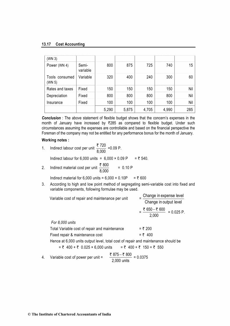
13.17 Cost Accounting
(WN 3)
Power (WN 4) Semi-
variable
800 875 725 740 15
Tools consumed
(WN 5)
Variable 320 400 240 300 60
Rates and taxes Fixed 150 150 150 150 Nil
Depreciation Fixed 800 800 800 800 Nil
Insurance Fixed 100 100 100 100 Nil
5,290 5,875 4,705 4,990 285
Conclusion : The above statement of flexible budget shows that the concern’s expenses in the
month of January have increased by `285 as compared to flexible budget. Under such
circumstances assuming the expenses are controllable and based on the financial perspective the
Foreman of the company may not be entitled for any performance bonus for the month of January.
Working notes :
1. Indirect labour cost per unit ` 720
8,000 =0.09 P.
Indirect labour for 6,000 units = 6,000 × 0.09 P = ` 540.
2. Indirect material cost per unit ` 800
8,000 = 0.10 P
Indirect material for 6,000 units = 6,000 × 0.10P = ` 600
3. According to high and low point method of segregating semi-variable cost into fixed and
variable components, following formulae may be used.
Variable cost of repair and maintenance per unit = leveloutput in Change
level expense in Change
= ` ` 650 600
2,000
= 0.025 P.
For 8,000 units
Total Variable cost of repair and maintenance = ` 200
Fixed repair & maintenance cost = ` 400
Hence at 6,000 units output level, total cost of repair and maintenance should be
= ` 400 + ` 0.025 × 6,000 units = ` 400 + ` 150 = ` 550
4. Variable cost of power per unit = ` `
875 800
2,000 units
= 0.0375
© The Institute of Chartered Accountants of India

Budgets and Budgetary Control 13.18
For 8,000 units
Total variable cost of power = ` 300
Fixed cost = ` 500
Hence, at 6,000 units output level, total cost of power should be
= ` 500 + ` 0.0375 × 6,000 units = ` 500 + ` 225 = ` 725
5. Tools consumed cost for 8,000 units = ` 320
Hence, tools consumed cost for 6,000 units = (` 320/8,000 units) × 6,000 units
= ` 240
Illustration- 4 (Preparation of flexible budget under incremental price)
ABC Ltd. is currently operating at 75% of its capacity. In the past two years, the levels of
operations were 55% and 65% respectively. Presently, the production is 75,000 units. The
company is planning for 85% capacity level during 20X3-20X4. The cost details are as follows:
55% 65% 75%
(` ) (` ) (` )
Direct Materials 11,00,000 13,00,000 15,00,000
Direct Labour 5,50,000 6,50,000 7,50,000
Factory Overheads 3,10,000 3,30,000 3,50,000
Selling Overheads 3,20,000 3,60,000 4,00,000
Administrative Overheads 1,60,000 1,60,000 1,60,000
24,40,000 28,00,000 31,60,000
Profit is estimated @ 20% on sales.
The following increases in costs are expected during the year :
In percentage
Direct Materials 8
Direct Labour 5
Variable Factory Overheads 5
Variable Selling Overheads 8
Fixed Factory Overheads 10
Fixed Selling Overheads 15
Administrative Overheads 10
Prepare flexible budget for the period 20X3-20X4 at 85% level of capacity. Also ascertain profit
and contribution.
© The Institute of Chartered Accountants of India

13.19 Cost Accounting
Solution:
ABC Ltd.
Budget for 85% capacity level for the period 20X3-X4
Budgeted production (units) 85,000
Per Unit (`) Amount (`)
Direct Material (note 1) 21.60 18,36,000
Direct Labour (note 2) 10.50 8,92,500
Variable factory overhead (note 3) 2.10 1,78,500
Variable selling overhead (note 4) 4.32 3,67,200
Variable cost 38.52 32,74,200
Fixed factory overhead (note 3) 2,20,000
Fixed selling overhead (note 4) 1,15,000
Administrative overhead 1,76,000
Fixed cost 5,11,000
Total cost 37,85,200
Add : Profit 20% on sales or 25% on total cost 9,46,300
Sales 47,31,500
Contribution (Sales – Variable cost) 14,57,300
Working Notes :
1. Direct Materials :
75% Capacity ` 15,00,000 65% Capacity ` 13,00,000
65% Capacity ` 13,00,000 55% Capacity ` 11,00,000
10% change in capacity 2,00,000 10% change in capacity 2,00,000
For 10% increase in capacity, i.e., for increase by 10,000 units, the total direct material
cost regularly changes by ` 2,00,000
Direct material cost (variable) = ` 2,00,000 ÷ 10,000 = ` 20
After 8% increase in price, direct material cost per unit = ` 20 × 1.08 = ` 21.60
Direct material cost for 85,000 budgeted units = 85,000 × ` 21.60 = ` 18,36,000
2. Direct Labour :
75% Capacity ` 7,50,000 65% Capacity ` 6,50,000
65% Capacity ` 6,50,000 55% Capacity ` 5,50,000
10% change in capacity 1,00,000 10% change in capacity 1,00,000
© The Institute of Chartered Accountants of India

Budgets and Budgetary Control 13.20
For 10% increase in capacity, direct labour cost regularly changes by ` 1,00,000.
Direct labour cost per unit = ` 1,00,000 ÷ 10,000 = ` 10
After 5% increase in price, direct labour cost per unit = ` 10 × 1.05 = ` 10.50
Direct labour for 85,000 units = 85,000 units × ` 10.50 = ` 8,92,500.
3. Factory overheads are semi-variable overheads:
75% Capacity ` 3,50,000 65% Capacity ` 3,30,000
65% Capacity ` 3,30,000 55% Capacity ` 3,10,000
10% change in capacity 20,000 10% change in capacity 20,000
Variable factory overhead = ` 20,000 ÷ 10,000 = ` 2
Variable factory overhead for 75,000 units = 75,000 × ` 2 = ` 1,50,000
Fixed factory overhead = ` 3,50,000 – ` 1,50,000 = ` 2,00,000.
Variable factory overhead after 5% increase = ` 2 × 1.05 = ` 2.10
Fixed factory overhead after 10% increase = ` 2,00,000 × 1.10 = ` 2,20,000.
4. Selling overhead is semi-variable overhead :
75% Capacity ` 4,00,000 65% Capacity ` 3,60,000
65% Capacity ` 3,60,000 55% Capacity ` 3,20,000
10% change in capacity 40,000 10% change in capacity 40,000
Variable selling overhead = ` 40,000 ÷ 10,000 units = ` 4
Variable selling overhead for 75,000 units = 75,000 × ` 4 = ` 3,00,000.
Fixed selling overhead = ` 4,00,000 – ` 3,00,000 = ` 1,00,000
Variable selling overhead after 8% increase = ` 4 × 1.08 = ` 4.32
Fixed selling overhead after 15% increase = ` 1,00,000 × 1.15 = ` 1,15,000
5. Administrative overhead is fixed :
After 10% increase = ` 1,60,000 × 1.10 = ` 1,76,000
13.8.2 Classification on the basis of Function:-
A functional budget is one which is related to function of the business as for example, production
budget relating to the manufacturing function. Functional budgets are prepared for each function
and they are subsidiary to the master budget of the business.
The various types of functional budgets to be prepared will vary according to the size and nature
of the business.
© The Institute of Chartered Accountants of India

13.21 Cost Accounting
The various commonly used functional budgets are:
(i) Sales budget
(ii) Production budget
(iii) Plant utilisation budget
(iv) Direct-material usage budget
(v) Direct-material purchase budget
(vi) Direct-labour (personnel) budget
(vii) Factory overhead budget
(viii) Production cost budget
(ix) Ending-inventory budget
(x) Cost-of-goods-sold budget
(xi) Selling and distribution cost budget
(xii) Administration expenses budget
(xiii) Research and development cost budget
(xiv) Capital expenditure budget
(xv) Cash budget
The important functional budgets (also known as schedules to master budget) and the master
budget are discussed and illustrated below:
(i) Sales Budget :
Sales forecast is the commencement of budgeting and hence sales budget assumes
primary importance. The quantity which can be sold may be the principal budget factor
in many business undertakings. In any case in order to chalk out a realistic budget
programme, there must be an accurate sales forecast.
The sales budget indicates for each product :
1. the quantity of estimated sales and
2. the expected unit selling price. These data are often reported by regions or by
sales representatives.
In estimating the quantity of sales for each product, past sales volumes are often
used as a starting point. These amounts are revised for factors that are expected to
affect future sales, such as the factors listed below.
(i) backlog of unfilled sales orders
(ii) planned advertising and promotion
© The Institute of Chartered Accountants of India

Budgets and Budgetary Control 13.22
(iii) expected industry and general economic conditions
(iv) productive capacity
(v) projected pricing
(vi) findings of market research studies
(vii) relative product profitability.
(viii) competition.
Once an estimate of the sales volume is obtained, the expected sales revenue can
be determined by multiplying the volume by the expected unit sales price. The sales
budget represents the total sales in physical quantities and values for a future budget
period. Sales managers are constantly faced with problem like anticipation of
customer requirements, new product needs, competitor strategies and various
changes in distribution methods or promotional techniques.
The purposes of sales budget is not to attempt to estimate or guess what the actual
sales will be, but rather to develop a plan with clearly defined objectives towards
which the operational effort is directed in order to attain or exceed the objective.
Hence, sales budget is not merely a sales forecast. A budget is a planning and control
document which shows what the management intends to accomplish. Thus, the sales
budget is active rather than passive.
A sales forecast, however, is a projection or estimate of the available customer
demand. A forecast reflects the environmental or competitive situation facing the
company whereas the sales budget shows how the management intends to react to
this environmental and competitive situation.
A good budget hinges on aggressive management control rather than on passive
acceptance of what the market appears to offer. If the company fails to make this
distinction, the budget will remain more a figure-work exercise than a working tool of
dynamic management control.
The sales budget may be prepared under the following classification or
combination of classifications :
1. Products or groups of products.
2. Areas, towns, salesmen and agents.
3. Types of customers as for example: (i) Government, (ii) Export, (iii) Home sales,
(iv) Retail depots.
4. Period—months, weeks, etc.
© The Institute of Chartered Accountants of India
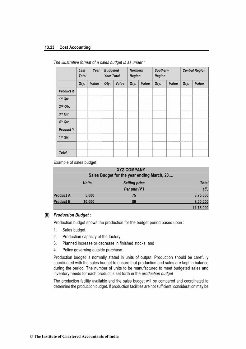
13.23 Cost Accounting
The illustrative format of a sales budget is as under :
Last Year
Total
Budgeted
Year Total
Northern
Region
Southern
Region
Central Region
Qty. Value Qty. Value Qty. Value Qty. Value Qty. Value
Product X
1st Qtr.
2nd Qtr.
3rd Qtr.
4th Qtr.
Product Y
1st Qtr.
:
Total
Example of sales budget:
XYZ COMPANY
Sales Budget for the year ending March, 20....
Units Selling price Total
Per unit (` ) (` )
Product A 5,000 75 3,75,000
Product B 10,000 80 8,00,000
11,75,000
(ii) Production Budget :
Production budget shows the production for the budget period based upon :
1. Sales budget,
2. Production capacity of the factory,
3. Planned increase or decrease in finished stocks, and
4. Policy governing outside purchase.
Production budget is normally stated in units of output. Production should be carefully
coordinated with the sales budget to ensure that production and sales are kept in balance
during the period. The number of units to be manufactured to meet budgeted sales and
inventory needs for each product is set forth in the production budget
The production facility available and the sales budget will be compared and coordinated to
determine the production budget. If production facilities are not sufficient, consideration may be
© The Institute of Chartered Accountants of India

Budgets and Budgetary Control 13.24
given to such factors as working overtime, introducing shift working, sub-contracting or
purchasing of additional plant and machinery. If, however, the production facilities are surplus,
consideration should be given to promote advertising, reduction of prices to increase the sales,
sub-contracting of surplus capacity, etc.
One of the conditions to be considered in all the compilation of production budget is the
level of stock to be maintained.
The level of stocks will depend upon three factors viz. :
1. seasonal industries in which stocks have to be built up during off season to cater to
the peak season,
2. a steady and uniform level of production to utilise the plant fully and to avoid
retrenchment or lay-off of the workers, and
3. to produce in such a way that minimum stocks are maintained at any time to avoid
locking up of funds in inventory.
Production budget can, therefore, show :
1. stabilised production every month, say, the maximum possible production or
2. stabilised minimum quantity of stocks which will reduce inventory costs.
3. In the case of stabilised production, the production facility will be fully utilised but the
inventory carrying costs will vary according to stocks held. In the case of stabilised
stocks method, however, the inventory carrying will be the lowest but there may be
under-utilisation of capacity.
Example of production budget:
XYZ COMPANY
Production budget in units for the year ending March 31, 20....
Products
A B
Budgeted sales 5,000 10,000
Add : Desired closing stock 500 1,000
Total quantity required 5,500 11,000
Less : Opening stock 1,500 2,000
Units to be produced 4,000 9,000
(iii) Plant Utilisation Budget:
Plant utilisation budget represents, in terms of working hours, weight or other convenient
units of plant facilities required to carry out the programme laid down in the production
budget.
© The Institute of Chartered Accountants of India

13.25 Cost Accounting
The main purposes of this budget are :
1. To determine the load on each process, cost or groups of machines for the budget period.
2. To indicate the processes or cost centres which are overloaded so that corrective
action may be taken such as: (i) working overtime (ii) sub-contracting (iii) expansion
of production facility, etc.
3. To dovetail the sales production budgets where it is not possible to increase the
capacity of any of the overloaded processes.
4. Where surplus capacity is available in any of the processes, to make effort to boost
sales to utilise the surplus capacity.
(iv) Direct Material usage Budget:
The steps involved in the compilation of direct materials usage budget are as under:
1. The quality standards for each item of material have to be specified. In this connection, standardisation of size, quality, colour, etc., may be considered.
2. Standard requirement of each item of materials required should also be set. While setting the standard quality consideration should be given to normal loss in process. The standard allowance for normal loss may be given on the basis of past performance, test runs, technical estimates etc.
3. Standard prices for each item of materials should be set after giving consideration to stock and contracts entered into.
After setting standards for quality, quantity and prices, the direct materials budget can be prepared by multiplying each item of material required for the production by the standard price.
Example of direct material usage budget is as under:
XYZ COMPANY
Direct material usage in units and in amount for the year ending March 31, 20...
Direct Materials
Type of materialProduct A Product B Total direct Material Total cost
(4,000 units) (9,000 units) material cost per of material
usage (Units) unit (` ) used (` )
X (12 units per
finished product) 48,000 1,08,000 1,56,000 1.50 2,34,000
Y (4 units per
product A & 2
units per product B)16,000 18,000 34,000 2.50 85,000
Total 3,19,000
© The Institute of Chartered Accountants of India

Budgets and Budgetary Control 13.26
(v) Purchase Budget:
The production budget is the starting point for determining the estimated quantities of
direct materials to be purchased.
Multiplying these quantities by the expected unit purchase price determines the total
cost of direct materials to be purchased.
Two important considerations that govern purchase budgets are as follows:
(i) Economic order quantity.
(ii) Re-order point with safety stocks to cover fluctuations in demand.
The direct material purchases budget helps management maintain inventory levels
within reasonable limits, For this purpose, the timing of the direct materials purchases
should he coordinated between the purchasing and production departments.
An example of material purchase budget is as under :
XYZ Company
Direct material purchase budget
for the year ending March 31, 20.....
Material X Material Y Total
Desired closing stock (units) 3,000 500
Units required for production 1,56,000 34,000
Add :
Total needs 1,59,000 34,500
Less: Opening stock (units) 4,000 300
Units to be purchased 1,55,000 34,200
Unit price (` ) 1.50 2.50
Purchase cost (` ) 2,32,500 85,500 3,18,000
(vi) Personnel (or Labour cost) Budget:
Once sales budget and Production budget are compiled and thereafter plant
utilisation budget is settled, detailed amount of the various machine operations in-
volved and services required can be arrived at. This will facilitate preparation of an
estimate of different grades of labour required.
From this the standard hours required to be worked can be prepared. The total labour
complement thus budgeted can be divided into direct and indirect. Standard rates of wages
for each grade of labour can be introduced and then the direct and indirect labour cost
budget can be prepared.
© The Institute of Chartered Accountants of India

13.27 Cost Accounting
Merits/advantages:
1. It defines the direct and indirect labour force required.
2. It enables the personnel department to plan ahead in recruitment and training of
workers so that labour turnover can be reduced to the minimum.
3. It reveals the labour cost to be incurred in the manufacture, to facilitate preparation
of manufacturing cost budgets and cash budgets for financing the wage bill.
Example of direct-labour cost budget:
XYZ COMPANY
Direct-labour cost budget
for the year ending March 31, 20...
Units to be Direct labour Total Total budget cost (` )
produced hour, per unit hours @ ` 2 per hour
Product A 4,000 7 28,000 56,000
Product B 9,000 10 90,000 1,80,000
1,18,000 2,36,000
(vii) Production or Factory overhead Budget:
Production overheads consist of all items such as indirect materials, indirect labour
and indirect expenses. Indirect expenses include power, fuel, fringe benefits,
depreciation etc. These estimated factory overhead costs necessary for production
make up the factory overhead cost budget.
This budget usually includes the total estimated cost for each item of factory
overhead.
The production overhead budget is useful for working out the pre-determined over-
head recovery rates.
A business may prepare supporting departmental schedules, in which the factory
overhead costs are separated into their fixed and variable cost elements. Such sched-
ules enable department managers to direct their attention to those costs for which
they are responsible and to evaluate performance
A careful study and determination of the behaviour of different types of costs will be
essential in preparation of overhead budget.
A few examples are given below to show how the expenses are estimated.
1. Fixed expenses are policy cost and hence they are based on policy matters.
2. For estimating indirect labour, work study is resorted to and a flexible estimate
© The Institute of Chartered Accountants of India
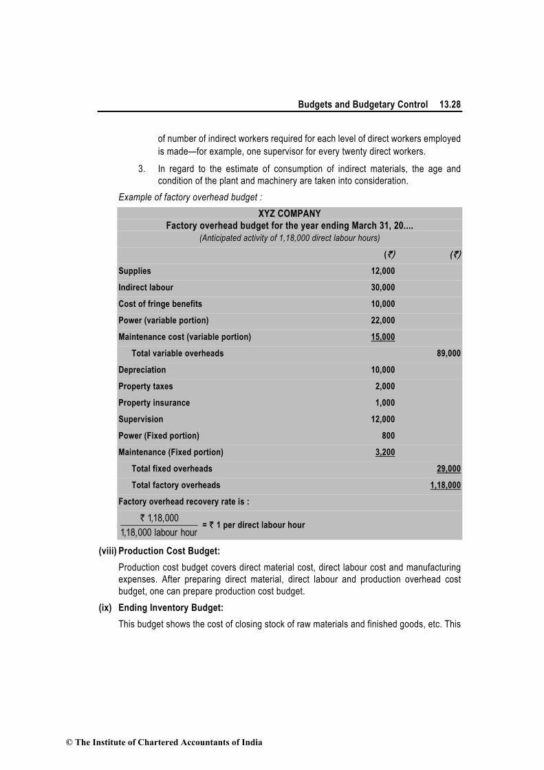
Budgets and Budgetary Control 13.28
of number of indirect workers required for each level of direct workers employed
is made—for example, one supervisor for every twenty direct workers.
3. In regard to the estimate of consumption of indirect materials, the age and
condition of the plant and machinery are taken into consideration.
Example of factory overhead budget :
XYZ COMPANY
Factory overhead budget for the year ending March 31, 20....
(Anticipated activity of 1,18,000 direct labour hours)
(`) (`)
Supplies 12,000
Indirect labour 30,000
Cost of fringe benefits 10,000
Power (variable portion) 22,000
Maintenance cost (variable portion) 15,000
Total variable overheads 89,000
Depreciation 10,000
Property taxes 2,000
Property insurance 1,000
Supervision 12,000
Power (Fixed portion) 800
Maintenance (Fixed portion) 3,200
Total fixed overheads 29,000
Total factory overheads 1,18,000
Factory overhead recovery rate is :
`
s
1,18,000
1,18,000 labour hour = ` 1 per direct labour hour
(viii) Production Cost Budget:
Production cost budget covers direct material cost, direct labour cost and manufacturing
expenses. After preparing direct material, direct labour and production overhead cost
budget, one can prepare production cost budget.
(ix) Ending Inventory Budget:
This budget shows the cost of closing stock of raw materials and finished goods, etc. This
© The Institute of Chartered Accountants of India

13.29 Cost Accounting
information is required to prepare cost-of-goods-sold budget and budgeted financial
statements i.e., budgeted income statement and budgeted balance sheet.
Example of ending inventory budget :
XYZ Company ending-inventory budget March 31, 20....
Units Unit cost Amount Total
(`) (`) (`)
Direct material
X 3,000 1.50 4,500
Y 500 2.50 1,250 5,750
Finished goods
A 500 49.00* 24,500
B 1,000 53.00* 53,000 77,500
Total 83,250
* Unit cost of finished goods have been computed as below :
Unit cost Product A Product B
of input Units Amount Units Amount
(` ) (` ) (` )
Material X 1.50 12 18.00 12.00 18.00
Material Y 2.50 4 10.00 2.00 5.00
Direct labour 2.00 7 14.00 10.00 20.00
Factory overhead 1.00 7 7.00 10.00 10.00
49.00 53.00
(x) Cost of Goods Sold Budget:
This budget covers direct material cost, direct labour cost, manufacturing expenses and
cost of ending inventory of finished products.
We present below the cost-of-goods-sold budget on the basis of the data taken from the
various budgets already illustrated:
XYZ Company cost-of-goods-sold budget for the year ending March 31, 20....
Amount
(`)
Direct materials used 3,19,000
Direct labour 2,36,000
© The Institute of Chartered Accountants of India

Budgets and Budgetary Control 13.30
Factory overhead 1,18,000
Total manufacturing costs 6,73,000
Add : Finished goods (opening) 1,79,500*
8,52,500
Less : Finished goods (closing) 77,500*
Total cost of goods sold 7,75,000
*Assumed figure
In the above budget if adjustments for opening and closing inventory of finished goods are
not shown. The budget will be called production cost budget.
(xi) Selling and Distribution Cost Budget:
Selling and distribution are indispensable aspects of the profit earning function. At the
same time, the pre-determination of these costs is also very difficult.
Selling cost is defined as the cost of seeking to create and stimulate demand and of
securing orders. These costs are, therefore, incurred to maintain and increase the
level of sales. All expenses connected with advertising, sales promotion, sales office,
salesmen, credit collection, market research, after sales service, etc. are generally
grouped together to form part of the responsibility of the sales manager.
While making a budget, selling costs are divided into fixed and variable. Semi-variable
costs should also be separated into variable and fixed elements.
The problems faced in the preparation of selling cost budgets are :
1. Heavy expenditure on selling and sales promotion may have to be incurred when
the volume of sales is falling off. This will increase the percentage of such costs
to total sales, and
2. Sometimes intensive sales and promotion efforts are called for in one year and
the benefit of such efforts accrue in the subsequent years. This makes it difficult
to establish a proportion of selling cost to sales.
3. In spite of these problems, some relationship between selling cost and volume
of sales has to be established and it is the duty of the Budget Controller to
determine the amount of selling costs to be incurred to achieve the desired level
of sales volume.
Using the past experience as a guide, consideration should be given to the future
trend of sales, possible changes in competition etc., in pre-determination of selling
costs.
Distribution cost has been defined as the cost of the sequence of operations which
begins with making the packet of product available for despatch and ends with making
the re-conditioned return of empty package, if any available for re-use. It includes
© The Institute of Chartered Accountants of India

13.31 Cost Accounting
transport cost, storage and warehousing costs, etc.
Preparation of the advertising cost budget is the responsibility of the sales manager
or advertisement manager. When preparing the advertisement cost budget
consideration should be given to the following factors :
1. The best method of advertisement must be selected; costs will vary according
to the method selected.
2. The maximum amount to be spent in a period, say one year, has to be decided.
3. Advertising and sales should be co-ordinated. It means that money should be
spent on advertisement only when sufficient quantities of the product advertised
are ready for sale.
4. An effective control over advertisement expenditure should be exercised and the
effectiveness of the advertisement should be measured.
5. The choice of the method of advertising a product is based on the effectiveness
of the money spent on advertisement in increasing or maintaining sales. If the
output sold increases, the production cost will come down because of the
economies of large scale production.
The amount to be spent on advertisement appropriation may be settled on the basis
of the following factors:
1. A percentage on the total sales value of the budget period or on the expected
profit may be fixed on the basis of past experience.
2. A sum which is expected to be incurred by the competitors may be fixed to be
spent during the budget period.
3. A fixed sum per unit of output can be fixed and added to cost.
4. An amount is fixed on the basis of the ability of the company to spend on
advertising.
5. An advertisement plan is decided upon and the amount to be spent is
determined.
Depending upon the nature of the product and the effectiveness of the media of the
advertising the company prepares a schedule of various methods of advertisement,
to be used for effective sales promotion. The number of advertisements (insertions)
are determined and the cost calculated as per the rates applicable to each of the
media selected. This is a sound method.
© The Institute of Chartered Accountants of India

Budgets and Budgetary Control 13.32
Example of selling and distribution cost budget:
XYZ Company selling and distribution cost budget
for the year ending March 31, 20....
Amount
Direct selling expenses: (`)
Salesmen’s salaries 14,500
Salesmen’s commission 7,000
Travelling expenses 19,000
40,500
Distribution expenses:
Warehouse wages 6,000
Warehouse rent, rates, electricity 4,500
Lorry expenses 11,000
21,500
Sales office expenses:
Salaries 16,000
Rent, rates, electricity 12,000
Depreciation 2,000
Stationery, postage and telephone 12,500
General expenses 3,000
45,500
Advertising:
Press 4,500
Radio and television 18,500
Shop window displays 4,000
27,000
Total 1,34,500
(xii) Administrative expenses Budget:
The administrative expenses are mostly policy costs and are, therefore, fixed in nature.
The most practical method to follow in preparing estimate of these expenses is to follow
the past experience with due regard to anticipated changes either in general policy or the
volume of business. To bring such expenses under control, it is necessary to review them
frequently and to determine at regular intervals whether or not these expenses continue to
be adjusted. Examples of such expenses are : audit fees, depreciation of office equipment,
insurance, subscriptions, postage, stationery, telephone, telegrams, office supplies, etc.
© The Institute of Chartered Accountants of India

13.33 Cost Accounting
XYZ Company administrative expenses budget for the year ending March 31, 20...
(`)
Salaries of clerical staff 28,000
Executives salaries 8,000
Audit fee 600
Depreciation on office equipment 800
Insurance 250
Stationery 1,250
Postage and telegrams 950
Telephones 850
Miscellaneous 5,300
Total administrative expenses 46,000
(xiii) Research and Development expense Budget:
Research is required in order to develop and/or improve products and methods. When research results in definite benefit to the company, development function begins. After development, formal production can commence on commercial scale and then production function starts. Since the areas of research and development cannot be precisely defined, the costs incurred under both the functions are clubbed together as research and development costs. Research and Development (R & D) plays a vital role in maintaining the business. For example, automobile manufacturers, and those who produce drugs, spend considerable sums on R & D to improve the products.
Research may be either pure research or applied research. Pure research increases knowledge whereas applied research aims at producing definite results like improved methods of production, etc.
Research and development expenses should be controlled carefully and hence a limit on the spending is placed, i.e., the amount to be spent is carefully determined or allocated.
The following are the methods of allocation of R & D expenses.
1. A percentage based on total sales value. This method is good if sales value is steady from year to year.
2. A percentage based on net profit.
3. A total sum is estimated on the basis of past experience and future R & D plans and policies.
4. A sum is fixed on the basis of cash resources available with the company.
All factors which affect the importance of R & D are considered. For example, factors like demand for existing products, competition, economic conditions, etc., are considered carefully and a sum is set as R & D budget.
© The Institute of Chartered Accountants of India
Budgets and Budgetary Control 13.34
(xiv) Capital expenditure Budget:
The capital expenditure budget represents the planned outlay on fixed assets like land, building, plant and machinery, etc. during the budget period. This budget is subject to strict management control because it entails large amount of expenditure. The budget is prepared to cover a long period of years and it projects the capital costs over the period in which the expenditure is to be incurred and the expected earnings.
The preparation of this budget is based on the following considerations :
1. Overhead on production facilities of certain departments as indicated by the plant utilisation budget.
2. Future development plans to increase output by expansion of plant facilities.
3. Replacement requests from the concerned departments
4. Factors like sales potential to absorb the increased output, possibility of price reductions, increased costs of advertising and sales promotion to absorb increased output, etc.
Merits/Advantages
1. It outlines the capital development programme and estimated capital expenditure during the budget period.
2. It enables the company to establish a system of priorities. When there is a shortage of funds, capital rationing becomes necessary.
3. It serves as a tool for controlling expenditure.
4. It provides the amount of expenditure to be incorporated in the future budget summaries for calculation of estimated return on capital employed.
5. This enables the cash budget to be completed. With other cash commitments capital expenditure commitment should also be considered for the completion of the budget.
6. It facilitates cost reduction programme, particularly when modernisation and renovation is covered by this budget.
Illustration 5: (Preparation of production budget)
A single product company estimated its sales for the next year quarter-wise as under :
Quarter Sales (Units)
I 30,000
II 37,500
III 41,250
IV 45,000
The opening stock of finished goods is 10,000 units and the company expects to maintain the closing stock of finished goods at 16,250 units at the end of the year. The production pattern in each quarter is based on 80% of the sales of the current quarter and 20% of the
© The Institute of Chartered Accountants of India

13.35 Cost Accounting
sales of the next quarter.
The opening stock of raw materials in the beginning of the year is 10,000 kg. and the closing stock at the end of the year is required to be maintained at 5,000 kg. Each unit of finished output requires 2 kg. of raw materials.
The company proposes to purchase the entire annual requirement of raw materials in the first three quarters in the proportion and at the prices given below :
Quarter Purchase of raw materials % to total Price per kg.
annual requirement in quantity (`) (`)
I 30% 2 II 50% 3 III 20% 4
The value of the opening stock of raw materials in the beginning of the year is ` 20,000. You are required to present the following for the next year, quarter wise :
(i) Production budget (in units).
(ii) Raw material consumption budget (in quantity).
(iii) Raw material purchase budget (in quantity and value).
(iv) Priced stores ledger card of the raw material using First in First out method.
Solution
Working Note : Total Annual Production (in units)
Sales in 4 quarters 1,53,750 units
Add : Closing balance 16,250 units
1,70,000 units
Less : Opening balance 10,000 units
Total number of units to be produced in the next year 1,60,000
(i) Production Budget (in units)
Quarters I II III IV Total Units Units Units Units Units
Sales 30,000 37,500 41,250 45,000 1,53,750 Production in current quarter 24,000 30,000 33,000 36,000 (80% of the sale of current quarter) Production for next quarter 7,500 8,250 9,000 12,250* (20% of the sale of next quarter) Total production 31,500 38,250 42,000 48,250 1,60,000
* Difference figure.
© The Institute of Chartered Accountants of India

Budgets and Budgetary Control 13.36
(ii) Raw material consumption budget in quantity
Quarters Total
I II III IV
Units to be produced in
each quarter: (A) 31,500 38,250 42,000 48,250 1,60,000
Raw material con-
sumption p.u. (kg.): (B) 2 2 2 2
Total raw material
consumption (Kg.) : (A × B) 63,000 76,500 84,000 96,500 3,20,000
(iii) Raw material purchase budget (in quantity)
Raw material required for production (kg.) 3,20,000
Add : Closing balance of raw material (kg.) 5,000
3,25,000
Less : Opening balance (kg.) 10,000
Material to be purchased (kg.) 3,15,000
Raw material purchase budget (in value)
Quarters % of annual require- Quantity of Rate per Amount
ment (Qty.) for pur- raw material kg.
chasing raw material to be purchased
(kg.) (` ) (` )
(1) (2) (3) (4) (5) = (3) × (4)
I 30 94,500 2 1,89,000
(3,15,000 kg. × 30%)
II 50 1,57,500 3 4,72,500
(3,15,000 kg. × 50%)
III 20 63,000 4 2,52,000
(3,15,000 kg. × 20%)
Total : 3,15,000 9,13,500
© The Institute of Chartered Accountants of India

13.37 Cost Accounting
(iv)
P
ric
ed
Sto
res
Le
dg
er
Ca
rd
(of
the
ra
w m
ate
ria
l u
sin
g F
IFO
me
tho
d)
Qu
art
ers
I II
II
I IV
Kg
. R
ate
V
alu
e
Kg
. R
ate
V
alu
e
Kg
. R
ate
V
alu
e
Kg
. R
ate
V
alu
e
(`)
(`)
(`)
(`)
(`)
(`)
(`)
(`)
Op
en
ing
ba
lan
ce
10
,00
0
2
20
,00
0
41
,50
0
2
83
,00
0
1,2
2,5
00
3
3
,67
,50
0
38
,50
0
3
1,1
5,5
00
(A)
6
3,0
00
4
2
,52
,00
0
Pu
rch
ase
s :
(B)
94
,50
0
2
1,8
9,0
00
1
,57
,50
0
3
4,7
2,5
00
6
3,0
00
4
2
,52
,00
0
–
–
–
Co
nsu
mp
tion
: (
C)
63
,00
0
2
1,2
6,0
00
4
1,5
00
2
8
3,0
00
8
4,0
00
3
2
,52
,00
0
38
,50
0
3
1,1
5,5
00
3
5,0
00
3
1
,05
,00
0
58
,00
0
4
2,3
2,0
00
Ba
lan
ce :
(D
) 4
1,5
00
2
8
3,0
00
1
,22
,50
0
3
3,6
7,5
00
3
8,5
00
3
1
,15
,50
0
5,0
00
4
2
0,0
00
(D)
= (
A)
+ (
B)–
(C)
63
,00
0
4
2,5
2,0
00
© The Institute of Chartered Accountants of India

Budgets and Budgetary Control 13.38
Illustration 6: (Preparation of production and personnel budget)
A company is engaged in the manufacture of specialised sub-assemblies required for
certain electronic equipments. The company envisages that in the forthcoming month,
December, 20X2, the sales will take a pattern in the ratio of 3 : 4 : 2 respectively of sub-
assemblies, ACB, MCB and DP.
The following is the schedule of components required for manufacture:
Component requirements
Sub-assembly Selling price Base board IC08 IC12 IC26
ACB 520 1 8 4 2
MCB 500 1 2 10 6
DP 350 1 2 4 8
Purchase price (`) 60 20 12 8
The direct labour time and variable overheads required for each of the sub-assemblies are:
Labour hours per sub-assembly
Grade A Grade B Variable overheads
per sub-assembly
(`)
ACB 8 16 36
MCB 6 12 24
DP 4 8 24
Direct wage rate per hour (`) 5 4 —
The labourers work 8 hours a day for 25 days a month.
The opening stocks of sub-assemblies and components for December, 20X2 are as under:
Sub-assemblies Components
ACB 800 Base Board 1,600
MCB 1,200 IC08 1,200
DP 2,800 IC12 6,000
IC26 4,000
Fixed overheads amount to ` 7,57,200 for the month and a monthly profit target of
` 12 lacs has been set.
The company is eager for a reduction of closing inventories for December, 20X2 of sub-
assemblies and components by 10% of quantity as compared to the opening stock.
Prepare the following budgets for December 20X2 :
(i) Sales budget in quantity and value.
© The Institute of Chartered Accountants of India

13.39 Cost Accounting
(ii) Production budget in quantity
(iii) Component usage budget in quantity.
(iv) Component purchase budget in quantity and value.
(v) Manpower budget showing the number of workers and the amount of wages payable.
Solution:
Working Note :
1. Statement showing contribution:
Sub assemblies ABC MCB DP Total
(`) (`) (`) (`)
Selling price per unit (p.u.) : (A) 520 500 350
Marginal Cost p.u.
Components
Base board 60 60 60
IC08 160 40 40
IC12 48 120 48
IC26 16 48 64
Labour
Grade A 40 30 20
Grade B 64 48 32
Variable production overhead 36 24 24
Total marginal cost p.u. : (B) 424 370 288
Contribution p.u. : (C) = (A) – (B) 96 130 62
Sales ratio : (D) 3 4 2
Contribution × Sales ratio : [(E) = (C) × (D)] 288 520 124 932
2. Desired Contribution for the forthcoming month December, 20X2
(`)
Fixed overheads 7,57,200
Desired profit 12,00,000
Desired contribution 19,57,200
3. Sales mix required i.e. number of batches for the forthcoming month December, 20X2
Sales mix required =Desired contribution/contribution × Sales ratio
=` 19,57,200/ 932 (Refer to Working notes 1 and 2)
= 2,100 batches
© The Institute of Chartered Accountants of India
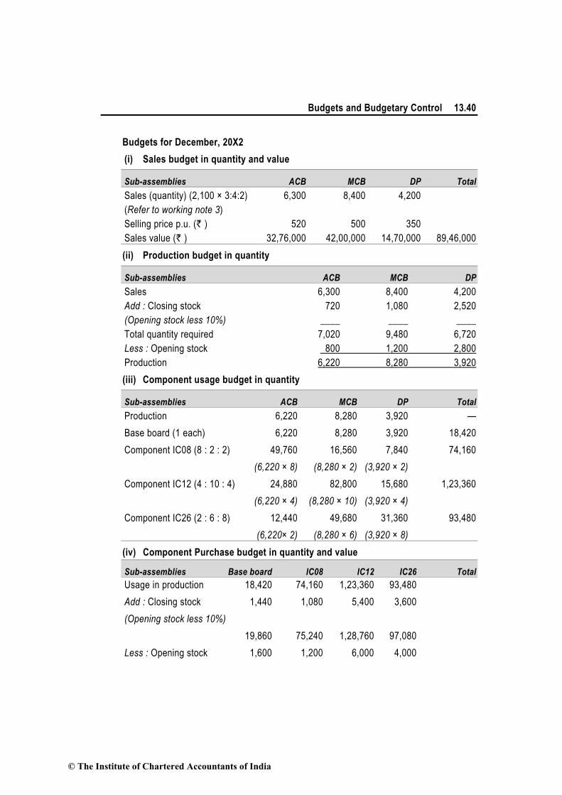
Budgets and Budgetary Control 13.40
Budgets for December, 20X2
(i) Sales budget in quantity and value
Sub-assemblies ACB MCB DP Total
Sales (quantity) (2,100 × 3:4:2) 6,300 8,400 4,200
(Refer to working note 3)
Selling price p.u. (` ) 520 500 350
Sales value (` ) 32,76,000 42,00,000 14,70,000 89,46,000
(ii) Production budget in quantity
Sub-assemblies ACB MCB DP
Sales 6,300 8,400 4,200
Add : Closing stock 720 1,080 2,520
(Opening stock less 10%) ____ ____ ____
Total quantity required 7,020 9,480 6,720
Less : Opening stock 800 1,200 2,800
Production 6,220 8,280 3,920
(iii) Component usage budget in quantity
Sub-assemblies ACB MCB DP Total
Production 6,220 8,280 3,920 —
Base board (1 each) 6,220 8,280 3,920 18,420
Component IC08 (8 : 2 : 2) 49,760 16,560 7,840 74,160
(6,220 × 8) (8,280 × 2) (3,920 × 2)
Component IC12 (4 : 10 : 4) 24,880 82,800 15,680 1,23,360
(6,220 × 4) (8,280 × 10) (3,920 × 4)
Component IC26 (2 : 6 : 8) 12,440 49,680 31,360 93,480
(6,220× 2) (8,280 × 6) (3,920 × 8)
(iv) Component Purchase budget in quantity and value
Sub-assemblies Base board IC08 IC12 IC26 Total
Usage in production 18,420 74,160 1,23,360 93,480
Add : Closing stock 1,440 1,080 5,400 3,600
(Opening stock less 10%)
19,860 75,240 1,28,760 97,080
Less : Opening stock 1,600 1,200 6,000 4,000
© The Institute of Chartered Accountants of India

13.41 Cost Accounting
Purchase (Quantity) 18,260 74,040 1,22,760 93,080
Purchase price (` ) 60 20 12 8
Purchase value (` ) 10,95,600 14,80,8 00 14,73,120 7,44,640 47,94,160
(v) Manpower budget showing the number of workers and the amount of wages
payable
Direct labour
Grade A Grade B
Sub- Budgeted Hours per Total Hours per Total Total
Assemblies Production Unit Hours Unit Hours
ACB 6,220 8 49,760 16 99,520
MCB 8,280 6 49,680 12 99,360
DP 3,920 4 15,680 8 31,360
(A) Total hours 1,15,120 2,30,240
(B) Hours per man per month 200 200
(C) Number of workers per month : (A/B) 576 1,152
(D) Wage rate per month (` ) 1,000 800
(E) Wages payable (` ) : (C × D) 5,76,000 9,21,600 14,97,600
(xv) Cash Budget :
Cash budget represents the cash requirements of the business during the budget
period. It is the plan of receipts and payments of cash for the budget period, analysed
to show the monthly flow of cash drawn up in such a way that the balance can be
forecasted at regular intervals.
The cash budget is one of the most important elements of the budgeted balance
sheet. Information from the various operating budgets, such as the sales budget, the
direct materials purchases budget, and the selling and administrative expenses
budget, affects the cash budget.
In addition, the capital expenditures budget, dividend policies, and plans for equity or
long-term debt financing also affect the cash budget.
13.8.3 Master Budget
When all the necessary functional budgets have been prepared, the budget officer will
prepare the master budget which may consist of budgeted profit and loss account and
budgeted balance sheet. These are in fact the budget summaries.
When the master budget is approved by the board of directors, it represents a standard for
the achievement of which all the departments will work.
© The Institute of Chartered Accountants of India

Budgets and Budgetary Control 13.42
On the basis of the various budgets (schedules) prepared earlier in this study, we prepare
below budgeted income statement and budgeted balance sheet.
Example of budgeted income statement:
XYZ Company Budgeted Income Statement
For the Year Ending March 31, 20....
Amount
(`) (`)
Sales 11,75,000
Less : Cost of goods sold 7,75,000
Gross margin 4,00,000
Less : Selling and distribution expenses 1,36,500
Less : Administrative expenses 46,000 1,82,500
Profit before interest and taxes 2,17,500
Interest expenses (assumed) 50,000
Profit before tax 1,67,500
Income-tax (50% assumed) 83,750
Net profit 83,750
Example of budgeted balance sheet :
XYZ Company Budgeted Balance Sheet
March 31, 20....
(`) (`) (`)
Share capital 3,50,000
Retained income 1,29,000 4,79,000
Represented by :
Plant and machinery 3,40,000
Less : Provision for depreciation 60,000 2,80,000
Raw materials 5,750
Finished goods 77,500
Debtors 1,10,000
Cash 37,750 2,31,000
Less: Creditors 32,000 1,99,000
4,79,000
Note : Information not available in respect of share capital, opening balance of retained earnings,
current assets and current liabilities, etc., has been assumed to complete the above balance
sheet.
© The Institute of Chartered Accountants of India

13.43 Cost Accounting
Illustration 7: (Preparation of Master Budget)
Floatglass Manufacturing Company requires you to present the Master budget for the next year
from the following information:
Sales :
Toughened Glass ` 6,00,000
Bent Glass ` 2,00,000
Direct material cost 60% of sales
Direct wages 20 workers @ ` 150 per month
Factory overheads :
Indirect labour –
Works manager ` 500 per month
Foreman ` 400 per month
Stores and spares 2.5% on sales
Depreciation on machinery ` 12,600
Light and power ` 3,000
Repairs and maintenance ` 8,000
Others sundries 10% on direct wages
Administration, selling and distribution expenses ` 36,000 per year
Solution:
Master Budget for the year ending
Sales : (`)
Toughened Glass 6,00,000
Bent Glass 2,00,000
Total Sales 8,00,000
Less : Cost of production :
Direct materials (60% of ` 8,00,000) 4,80,000
Direct wages (20 workers × ` 150 × 12 months) 36,000
Prime Cost 5,16,000
Fixed Factory Overhead :
Works manager’s salary (500 × 12) 6,000
Foreman’s salary (400 × 12) 4,800
Depreciation 12,600
© The Institute of Chartered Accountants of India

Budgets and Budgetary Control 13.44
Light and power (assumed fixed) 3,000 26,400
Variable Factory Overhead :
Stores and spares 20,000
Repairs and maintenance 8,000
Sundry expenses 3,600 31,600
Works Cost 5,74,000
Gross Profit (Sales – Works cost) 2,26,000
Less: Adm., selling and distribution expenses 36,000
Net Profit 1,90,000
Illustration 8: (Preparation of Budget comparison of two periods)
The cost accountant of manufacturing company provides you the following details for year 20X2 :
(`) (`)
Direct materials 1,75,000 Other variable costs 80,000
Direct Wages 1,00,000 Other fixed costs 80,000
Fixed factory overheads 1,00,000 Profit 1,15,000
Variable factory overheads 1,00,000 Sales 7,50,000
During the year, the company manufactured two products A and B and the output and costs
were :
A B
Output (units) 2,00,000 1,00,000
Selling price per unit ` 2.00 ` 3.50
Direct materials per unit ` 0.50 ` 0.75
Direct wages per unit ` 0.25 ` 0.50
Variable factory overhead are absorbed as a percentage of direct wages. Other variable costs
have been computed as : Product A ` 0.25 per unit; and B ` 0.30 per unit.
During 20X3, it is expected that the demand for product A will fall by 25 % and for B by 50%. It
is decided to manufacture a further product C, the cost for which are estimated as follows :
Product C
Output (units) 2,00,000
Selling price per unit ` 1.75
Direct materials per unit ` 0.40
Direct wages per unit ` 0.25
© The Institute of Chartered Accountants of India

13.45 Cost Accounting
It is anticipated that the other variable costs per unit will be the same as for product A.
Prepare a budget to present to the management, showing the current position and the position
for 20X3. Comment on the comparative results.
Solution: Budget Showing Current Position and Position for 20X3
Position for 20X2 Position for 20X3
A B Total
(A+B)
A B C Total
(A+B+C)
Sales (units) 2,00,000 1,00,000 – 1,50,000 50,000 2,00,000 –
(`) (`) (`) (`) (`) (`) (`)
(A) Sales (` ) 4,00,000 3,50,000 7,50,000 3,00,000 1,75,000 3,50,000 8,25,000
Direct
Material
1,00,000 75,000 1,75,000 75,000 37,500 80,000 1,92,500
Direct wages 50,000 50,000 1,00,000 37,500 25,000 50,000 1,12,500
Factory
overhead
(variable)
50,000 50,000 1,00,000 37,500 25,000 50,000 1,12,500
Other variable
costs
50,000 30,000 80,000 37,500 15,000 50,000 1,02,500
(B) Marginal
Cost
2,50,000 2,05,000 4,55,000 1,87,500 1,02,500 2,30,000 5,20,000
(C)
Contribution
(A-B)
1,50,000 1,45,000 2,95,000 1,12,500 72,500 1,20,000 3,05,000
Fixed costs –
Factory
1,00,000
1,00,000
– Others 80,000 80,000
(D) Total fixed
cost
1,80,000 1,80,000
Profit
(C – D)
1,15,000 1,25,000
Comments: Introduction of Product C is likely to increase profit by ` 10,000 (i.e. from ` 1,15,000 to `
1,25,000) in 20X3 as compared to 20X2. Therefore, introduction of product C is recommended.
© The Institute of Chartered Accountants of India

Budgets and Budgetary Control 13.46
13.8.4 Classification on the basis of Period:
These types of Budgets are classified on the basis of time periods. These types of budgets reflect
the planning period of the organization.
1. Long term Budget: - The Budgets are prepared to depict long term planning of the business.
The period of long term Budgets varies between three to ten years. These budgets are useful
for those industries where gestation period is long i.e., machinery, electricity etc.
2. Short term Budget: - These budgets are generally for one or two years and are in the form of
monetary terms. The consumer’s good industries like Sugar, Cotton, and textile use short term
budgets.
3. Current Budgets: - The period of current budgets is generally of months and weeks. These
budgets relate to the current activities of the business. According to CIMA London “Current
budget is a budget which is created which is established for use over a short period of time and
is related to current conditions”.
13.9 Summary
Budget: It is statement of an estimated performance to be achieved in given time, expressed
in currency value or quantity or both.
Budget Centre: A section of an organization for which separate budget can be prepared and
control exercised.
Budgetary Control: Guiding and regulating activities with a view to attaining predetermined
objectives, effectively and efficiently.
Budget Manual: The Budget manual is a schedule, document or booklet which shows, in
written forms the budgeting organisation and procedures.
Budget Period: The period of time for which a budget is prepared and used. It may be a year,
quarter or a month.
Components of Budgetary Control System are Physical budgets, Cost budgets, Profit
budgets and Financial budgets
Objectives of budgeting are Planning, Directing and Controlling
Classification of Budgets :
Nature based - Fixed and Flexible
Content based - Monetary and Physical
Functional based - Purchase, Sale, Production Cost, Administrative,
Selling & Distribution, Research & Development, Plant Capital
Expenditure, Cash, Plant Utilization
© The Institute of Chartered Accountants of India

INTERMEDIATE (IPC) COURSE
STUDY MATERIAL
PAPER : 3
COST ACCOUNTING AND
FINANCIAL MANAGEMENT Part – 1 : Cost Accounting
MODULE – 2
BOARD OF STUDIES
THE INSTITUTE OF CHARTERED ACCOUNTANTS OF INDIA
© The Institute of Chartered Accountants of India

ii
This Study Material has been prepared by the faculty of the Board of Studies. The objective of
the study material is to provide teaching material to the students to enable them to obtain
knowledge in the subject. In case students need any clarifications or have any suggestions to
make for further improvement of the material contained herein, they may write to the Director
of Studies.
All care has been taken to provide interpretations and discussions in a manner useful for the
students. However, the study material has not been specifically discussed by the Council of
the Institute or any of its Committees and the views expressed herein may not be taken to
necessarily represent the views of the Council or any of its Committees.
Permission of the Institute is essential for reproduction of any portion of this material.
© The Institute of Chartered Accountants of India
All rights reserved. No part of this book may be reproduced, stored in a retrieval system, or
transmitted, in any form, or by any means, electronic, mechanical, photocopying, recording, or
otherwise, without prior permission, in writing, from the publisher.
Revised Edition : April, 2016
Website : www.icai.org
E-mail : [email protected]
Committee/ : Board of Studies
Department
ISBN No. :
Price (All Modules) : `
Published by : The Publication Department on behalf of The Institute of
Chartered Accountants of India, ICAI Bhawan, Post Box No.
7100, Indraprastha Marg, New Delhi 110 002, India.
Printed by :
© The Institute of Chartered Accountants of India

iii
CONTENTS
MODULE – 1
Chapter 1 – Basic Concepts
Chapter 2 – Material
Chapter 3 – Labour
Chapter 4 – Overheads
MODULE – 2
Chapter 5 – Non Integrated Accounts
Chapter 6 – Job Costing and Batch Costing
Chapter 7 – Contract Costing
Chapter 8 – Operating Costing
Chapter 9 – Process & Operation Costing
Chapter 10 – Joint Products & By Products
Chapter 11 – Standard Costing
Chapter 12 – Marginal Costing
Chapter 13 – Budgets and Budgetary Control
© The Institute of Chartered Accountants of India

iv
DETAILED CONTENTS : MODULE – 2
CHAPTER 5 – NON INTEGRATED ACCOUNTS
5.1 Introduction .......................................................................................................................5.1
5.2 Non-Integrated Accounting System ..................................................................................5.1
5.3 Integrated (or Integral) Accounting System .................................................................... 5.30
5.4 Reconciliation of Cost and Financial Accounts .............................................................. 5.44
5.5 Summary ........................................................................................................................ 5.54
CHAPTER 6 – JOB COSTING AND BATCH COSTING
6.1 Methods of Costing...........................................................................................................6.1
6.2 Job Costing ......................................................................................................................6.2
6.3 Procedure of job Cost Accounting ....................................................................................6.4
6.4 Batch Costing ................................................................................................................. 6.13
6.5 Summary ........................................................................................................................ 6.18
CHAPTER 7 – CONTRACT COSTING
7.1 Introduction .......................................................................................................................7.1
7.2 Meaning of Contract Costing ............................................................................................7.1
7.3 Recording of contract costs ..............................................................................................7.2
7.4 Meaning of the terms used in contract costing .................................................................7.3
7.5 Profit/loss on incomplete contracts ...................................................................................7.5
7.6 Cost plus contract .............................................................................................................7.6
7.7 Summary ........................................................................................................................ 7.25
© The Institute of Chartered Accountants of India

v
CHAPTER 8 – OPERATING COSTING
8.1 Meaning of Operating Costing ..........................................................................................8.1
8.2 Unit of cost in Operating Costing ......................................................................................8.1
8.3 Preparation of Cost Sheet under Operating Costing ........................................................8.3
8.4 Standard Load ................................................................................................................ 8.15
8.5 Multiple Costing .............................................................................................................. 8.15
8.6 Summary ........................................................................................................................ 8.16
CHAPTER 9 – PROCESS & OPERATION COSTING
9.1 Meaning of Process Costing .............................................................................................9.1
9.2 Operation Costing.............................................................................................................9.2
9.3 Treatment of Normal Process Loss, Abnormal Process Loss and Abnormal Gain ..........9.4
9.4 Costing of Equivalent Production Units ............................................................................9.9
9.5 Inter-Process Profits ....................................................................................................... 9.21
9.6 Summary ........................................................................................................................ 9.23
CHAPTER 10 – JOINT PRODUCTS & BY PRODUCTS
10.1 Meaning of Joint Products and By-Products................................................................... 10.1
10.2 Apportionment of joint costs ........................................................................................... 10.2
10.3 Method of apportioning joint cost over joint products ..................................................... 10.2
10.4 Methods of apportioning joint cost over by-products .................................................... 10.13
10.5 Treatment of By-Product Cost in Cost-Accounting ....................................................... 10.14
10.6 Summary ...................................................................................................................... 10.15
CHAPTER 11 – STANDARD COSTING
11.1 Introduction ..................................................................................................................... 11.1
11.2 Standard Costing ............................................................................................................ 11.2
11.3 Setting Up of Standard Cost ........................................................................................... 11.2
© The Institute of Chartered Accountants of India

vi
11.4 Types of Standards ........................................................................................................ 11.7
11.5 Need for Standard Costs ................................................................................................ 11.8
11.6 The Process of Standard Costing ................................................................................... 11.8
11.7 Types of Variances ......................................................................................................... 11.9
11.8 Classification of Variances ............................................................................................. 11.9
11.9 Preparation of Operating Statement under Standard Costing –
Reporting of Variances ................................................................................................. 11.42
11.10 Accounting Procedure For Standard Cost .................................................................... 11.43
11.11 Disposition of Variances ............................................................................................... 11.45
11.12 Advantages and Criticism of Standard Costing ............................................................ 11.46
11.13 Summary ...................................................................................................................... 11.48
CHAPTER 12 – MARGINAL COSTING
12.1 Definitions ....................................................................................................................... 12.1
12.2 Characteristics of Marginal Costing ................................................................................ 12.3
12.3 Facts about Marginal Costing ......................................................................................... 12.4
12.4 Distinction between Marginal and Absorption Costing ................................................... 12.5
12.5 Advantages and Limitations of Marginal Costing .......................................................... 12.12
12.6 Cost-Volume-Profit Analysis ......................................................................................... 12.14
12.7 Methods of Break -Even Analysis ................................................................................. 12.16
12.8 Algebraic Calculations .................................................................................................. 12.16
12.9 Margin of Safety ........................................................................................................... 12.28
12.10 Variations of Basic Marginal Cost Equation and other formulae .................................. 12.28
12.11 Angle of Incidence ........................................................................................................ 12.39
12.12 Graphical Representation of Break Even Chart ............................................................ 12.40
12.13 The Limitations of Breakeven Analysis ......................................................................... 12.46
12.14 Summary ...................................................................................................................... 12.47
© The Institute of Chartered Accountants of India

vii
CHAPTER 13 – BUDGETS AND BUDGETARY CONTROL
13.1 Introduction ..................................................................................................................... 13.1
13.2 Meaning of Budget and Budgeting ................................................................................. 13.1
13.3 Essentials of Budget ....................................................................................................... 13.1
13.4 Characteristic of Budget ................................................................................................. 13.2
13.5 Objectives of Budgeting .................................................................................................. 13.2
13.6 Meaning of Budgetary Control ........................................................................................ 13.4
13.7 Preparation of Budgets ................................................................................................... 13.8
13.8 Different Types of Budgets ........................................................................................... 13.10
13.9 Summary ...................................................................................................................... 13.46
© The Institute of Chartered Accountants of India