Intermediate Macroeconomics, EC2201

L7: Government debt and sustainable fiscal policy

Anna Seim

Department of Economics, Stockholm University

Spring 2017

1 / 38

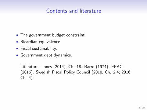
Contents and literature

• The government budget constraint.

• Ricardian equivalence.

• Fiscal sustainability.

• Government debt dynamics.

Literature: Jones (2014), Ch. 18. Barro (1974). EEAG(2016). Swedish Fiscal Policy Council (2010, Ch. 2,4; 2016,Ch. 4).

2 / 38

Extracted from: Jones (2014).

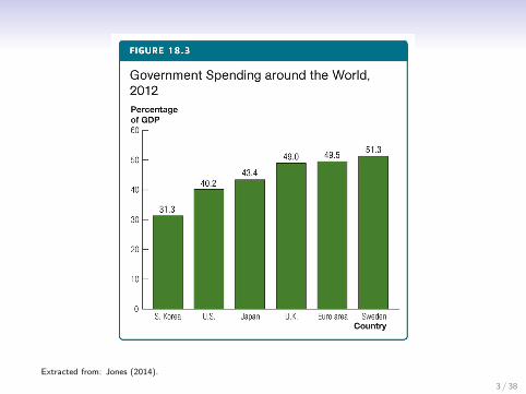
3 / 38

Extracted from: Jones (2014).

4 / 38

Extracted from: Jones (2014).

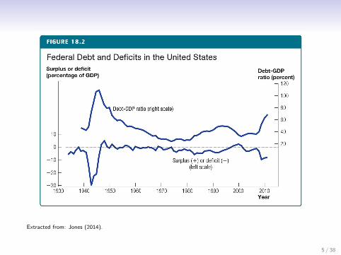
5 / 38

Extracted from: Jones (2014).

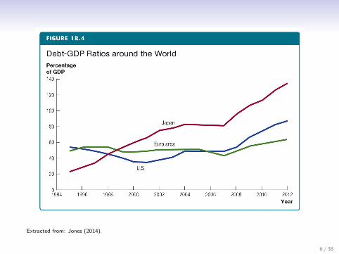
6 / 38

Ricardian equivalence

• Normally we expect lower taxes today to increase the realdisposable income of households and therefore increase privateconsumption.

• Under Ricardian Equivalence, households recognise that a taxcut today implies higher taxes in the future, leaving lifetimeincome unchanged.

• Under Ricardian Equivalence, private consumption isunaffected by a change in the tax rate.

7 / 38

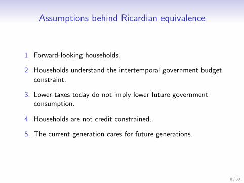
Assumptions behind Ricardian equivalence

1. Forward-looking households.

2. Households understand the intertemporal government budgetconstraint.

3. Lower taxes today do not imply lower future governmentconsumption.

4. Households are not credit constrained.

5. The current generation cares for future generations.

8 / 38

Ricardian equivalence in a two-period model

Notation:

Gt : government consumption in period t, t = 1,2.

Tt : tax revenue in period t.

D: the government budget deficit.

r : the interest rate.

9 / 38

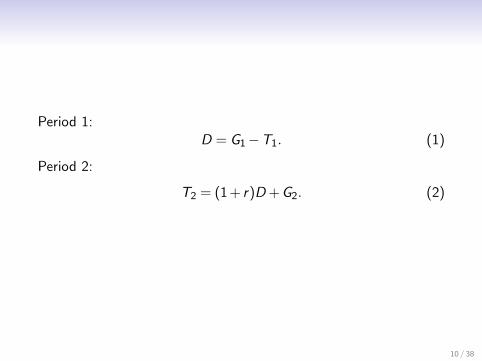
Period 1:D = G1−T1. (1)

Period 2:

T2 = (1 + r)D +G2. (2)

10 / 38

Substituting D from (1) in (2) we obtain:

T2 = (1 + r)(G1−T1) +G2. (3)

Re-arranging, the intertemporal government budget constraint canbe written:

T1 +T2

1 + r= G1 +

G2

1 + r. (4)

Equation (4) suggests that the present value of tax revenue andexpenditures must be equal.

11 / 38

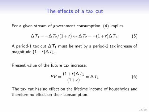
The effects of a tax cut

For a given stream of government consumption, (4) implies

∆T1 =−∆T2/(1 + r)⇔∆T2 =−(1 + r)∆T1. (5)

A period-1 tax cut ∆T1 must be met by a period-2 tax increase ofmagnitude (1 + r)∆T1.

Present value of the future tax increase:

PV =(1 + r)∆T1

(1 + r)= ∆T1 (6)

The tax cut has no effect on the lifetime income of households andtherefore no effect on their consumption.

12 / 38

The household’s perspective

Notation:

Yt : household income in period t, t = 1,2.

Ct : consumption in period t.

The household’s intertemporal budget constraint:

C1 +C2

1 + r= Y1 +

Y2

1 + r(7)

Equation (7) suggest that period-2 consumption prior to the taxcut must satisfy:

C2 = Y2 + (1 + r)(Y1−C1) (8)

13 / 38

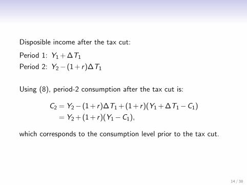
Disposible income after the tax cut:

Period 1: Y1 + ∆T1

Period 2: Y2− (1 + r)∆T1

Using (8), period-2 consumption after the tax cut is:

C2 = Y2− (1 + r)∆T1 + (1 + r)(Y1 + ∆T1−C1)

= Y2 + (1 + r)(Y1−C1),

which corresponds to the consumption level prior to the tax cut.

14 / 38

A temporary increase in government expenditure

• Consider a temporary increase in government expenditure,∆G1 > 0.

• Households anticipate a temporary future tax increase to payfor the higher G .

• The future tax increase lowers lifetime income, causinghouseholds to consume less, but because of consumptionsmoothing, the decrease in consumption in any given period issmall.

• Since ∆G1 > 0 and ∆C1 < 0, but the former dominates thelatter, a temporary increase in government expenditure willincrease aggregate demand in the current period.

15 / 38

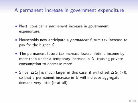
A permanent increase in government expenditure

• Next, consider a permanent increase in governmentexpenditure.

• Households now anticipate a permanent future tax increase topay for the higher G .

• The permanent future tax increase lowers lifetime income bymore than under a temporary increase in G , causing privateconsumption to decrease more.

• Since |∆C1| is much larger in this case, it will offset ∆G1 > 0,so that a permanent increase in G will increase aggregatedemand very little (if at all).

16 / 38

Two types of fiscal policy

Automatic stabilisers: automatic changes in tax revenue andgovernment expenditure occurring over the business cycle.

Discretionary fiscal policy: active decisions.

Consensus view in normal times: avoid discretionary measures, relyon automatic stabilisers.

17 / 38

Why are fiscal deficits potentially a problem?

1. Higher future taxes imply large distortionary costs.

• Distortionary costs rise more than proportionally to themarginal tax rate.

• Tax smoothing optimal.

2. Intergenerational redistribution.

• Interest payments are a transfer from future generations to thecurrent generation.

• Crowding out investments.

3. Risk of government default.

• Credit losses may trigger financial crises.• Defaulting country will be unable to borrow on financial

markets.

18 / 38

Deficit bias

Inherent tendency to accumulate government debt. Why?

1. Myopia.

2. More popular to lower taxes and increase governmentspending in recessions than raising taxes and reducingspending in booms.

3. Incumbent governments seek to favour their constituents.Running deficits ties the hands of future governments.

4. Common-pool problems: interest groups try to elicit favourswithout consideration for the costs of others.

5. Governments may seek to signal competency by combininghigh spending and low taxes if voters are uninformed.

19 / 38

Government debt dynamics

Notation:

Dt : government debt in period t.

Yt : nominal GDP.

γt : the nominal GDP growth rate.

it : the nominal interest rate.

Tt : tax revenue.

Gt : government expenditure (excluding interest payments).

St : the primary fiscal balance.

Bt : the fiscal balance.

20 / 38

Debt dynamics:Dt = Dt−1−Bt , (9)

where

Bt = Tt −Gt − itDt−1 = St − itDt−1. (10)

Using (10) in (9), we obtain:

Dt = Dt−1− (St − itDt−1) = (1 + it)Dt−1−St . (11)

21 / 38

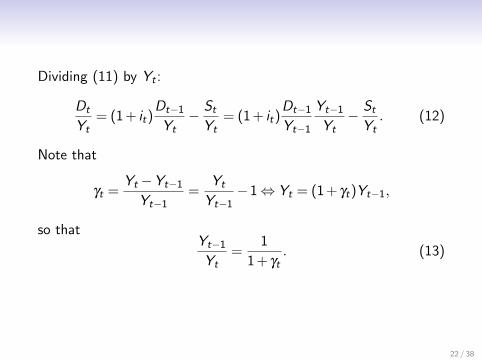
Dividing (11) by Yt :

Dt

Yt= (1 + it)

Dt−1

Yt− St

Yt= (1 + it)

Dt−1

Yt−1

Yt−1

Yt− St

Yt. (12)

Note that

γt =Yt −Yt−1

Yt−1=

Yt

Yt−1−1⇔ Yt = (1 + γt)Yt−1,

so thatYt−1

Yt=

1

1 + γt. (13)

22 / 38

Using (13) in (12), we obtain:

Dt

Yt=

(1 + it)

(1 + γt)

Dt−1

Yt−1− St

Yt,

or

dt =(1 + it)

(1 + γt)dt−1− st , (14)

where dt ≡ Dt/Yt is the debt-to-GDP ratio and st ≡ St/Yt .

23 / 38

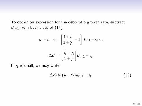
To obtain an expression for the debt-ratio growth rate, subtractdt−1 from both sides of (14):

dt −dt−1 =

[1 + it1 + γt

−1

]dt−1− st ⇔

∆dt =

[it − γt

1 + γt

]dt−1− st .

If γt is small, we may write:

∆dt ≈ (it − γt)dt−1− st . (15)

24 / 38

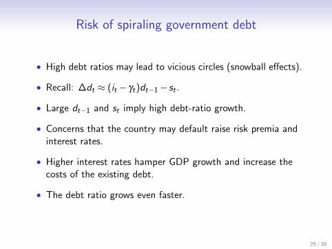
Risk of spiraling government debt

• High debt ratios may lead to vicious circles (snowball effects).

• Recall: ∆dt ≈ (it − γt)dt−1− st .

• Large dt−1 and st imply high debt-ratio growth.

• Concerns that the country may default raise risk premia andinterest rates.

• Higher interest rates hamper GDP growth and increase thecosts of the existing debt.

• The debt ratio grows even faster.

25 / 38

The fiscal consolidation-growth trade-off

• Equation (15) implies that if it − γt > 0, debt can only bestabilised if there is a primary surplus, st > 0.

• But a primary surplus requires fiscal consolidation (austerity).

• Austerity implies lower growth, which raises the debt ratio.

• Heated European debate in recent years on the effects of fiscalausterity.

26 / 38

Extracted from: EEAG (2016).27 / 38

Extracted from: EEAG (2016).

28 / 38

Fiscal sustainability

• Fiscal sustainability: the debt ratio must settle down at someconstant value.

• In addition to large debts in the aftermath of the recent crisis,ageing populations threaten fiscal sustainability in manycountries.

29 / 38

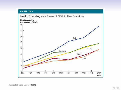
Extracted from: Jones (2014).

30 / 38

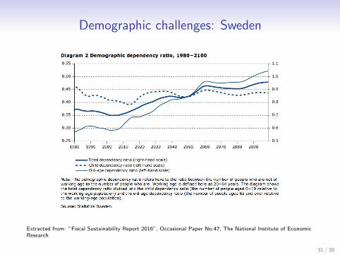
Demographic challenges: Sweden

Extracted from: ”Fiscal Sustainability Report 2016”, Occasional Paper No.47, The National Institute of EconomicResearch.

31 / 38

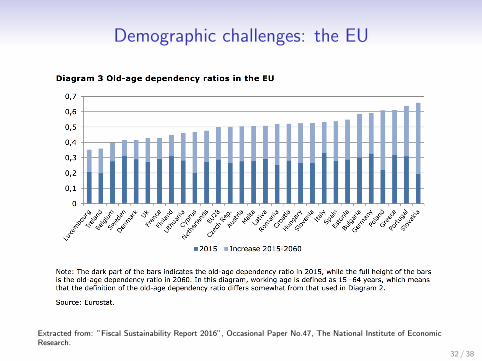
Demographic challenges: the EU

Extracted from: ”Fiscal Sustainability Report 2016”, Occasional Paper No.47, The National Institute of EconomicResearch.

32 / 38

Long-term fiscal sustainability

• Making assumptions about future growth, interest rates andemployment, and assuming unchanged transfer systems andpublic expenditure per capita, one can calculate how muchtaxes must increase relative to GDP to fund the ageingpopulation.

• The intertemporal government budget constraint: the netfinancial worth of the government ≥ the discounted value offuture primary deficits.

• Government bonds hold value only because they are backed bythe government’s ability to service its debt.

33 / 38

The S2-indicator

• The S2-indicator: the annual permanent budget improvementin per cent of GDP that would be needed to meet theintertemporal budget constraint.

• S2 > 0: Non-sustainable fiscal policy

• S2≤ 0: Sustainable fiscal policy

34 / 38

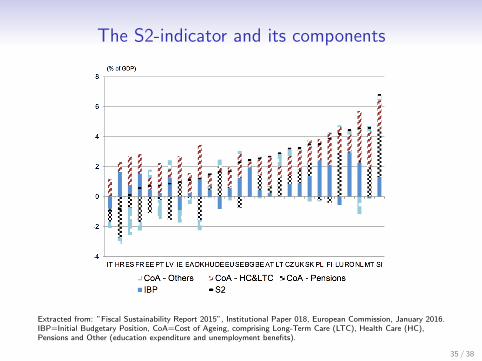
The S2-indicator and its components

Extracted from: ”Fiscal Sustainability Report 2015”, Institutional Paper 018, European Commission, January 2016.IBP=Initial Budgetary Position, CoA=Cost of Ageing, comprising Long-Term Care (LTC), Health Care (HC),Pensions and Other (education expenditure and unemployment benefits).

35 / 38

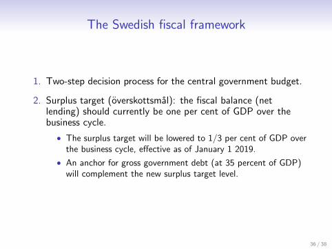
The Swedish fiscal framework

1. Two-step decision process for the central government budget.

2. Surplus target (overskottsmal): the fiscal balance (netlending) should currently be one per cent of GDP over thebusiness cycle.

• The surplus target will be lowered to 1/3 per cent of GDP overthe business cycle, effective as of January 1 2019.

• An anchor for gross government debt (at 35 percent of GDP)will complement the new surplus target level.

36 / 38

3. Ceiling for central government expenditure (utgiftstak) threeyears ahead. Comprises all expenditures including pensions,but excludes interest payments.

4. Balanced budget requirement for local governments:municipalities (kommuner) and regions (landsting).

5. Fiscal policy is monitored by independent institutions, inparticular the Swedish Fiscal Policy Council (Finanspolitiskaradet).

37 / 38

What we did

• The government budget constraint.

• Ricardian equivalence.

• Fiscal sustainability.

• Government debt dynamics.

Literature: Jones (2014), Ch. 18. Barro (1974). EEAG(2016). Swedish Fiscal Policy Council (2010, Ch. 2,4; 2016,Ch. 4).

38 / 38