1

1

Expected Utility

Health Economics

Fall 2016

2

Intermediate Micro

• Workhorse model of intermediate micro– Utility maximization problem

– Consumers Max U(x,y) subject to the budget constraint, I=Pxx + Pyy

• Problem is made easier by the fact that we assume all parameters are known– Consumers know prices and income

– Know exactly the quality of the product

– simple optimization problem

3

• Many cases, there is uncertainty about some variables– Uncertainty about income?

– What are prices now? What will prices be in the future?

– Uncertainty about quality of the product?

• This section, will review utility theory under uncertainty

4

• Will emphasize the special role of insurance in a generic sense– Why insurance is ‘good’ -- consumption smoothing across

states of the world– How much insurance should people purchase?

• Applications: Insurance markets may generate incentives that reduce the welfare gains of consumption smoothing– Moral hazard– Adverse selection

2

5

Definitions

• Probability - likelihood discrete event will occur– n possible events, i=1,2,..n

– Pi be the probability event i happens

– 0 ≤Pi≤1

– P1+P2+P3+…Pn=1

• Probabilities can be ‘subjective’ or ‘objective’, depending on the model

• In our work, probabilities will be know with certainty

6

• Expected value –– Weighted average of possibilities, weight is probability

– Sum of the possibilities times probabilities

• x={x1,x2…xn}

• P={P1,P2,…Pn}

• E(x) = P1X1 + P2X2 + P3X3 +….PnXn

7

• Roll of a die, all sides have (1/6) prob. What is expected roll?

• E(x) = 1(1/6) + 2(1/6) + … 6(1/6) = 3.5

• Suppose you have: 25% chance of an A, 50% B, 20% C, 4% D and 1% F

• E[quality points] = 4(.25) + 3(.5) + 2(.2) + 1(.04) + 0(.01) = 2.94

8

Expected utility

• Suppose income is random. Two potential values (Y1or Y2)

• Probabilities are either P1 or P2=1-P1

• When incomes are realized, consumer will experience a particular level of income and hence utility

• But, looking at the problem beforehand, a person has a particular ‘expected utility’

3

• However, suppose an agent is faced with choice between two different paths– Choice a: Y1 with probability P1 and Y2 with P2

– Choice b: Y3 with probability P3 and Y4 with P4

• Example: You are presented with two option– a job with steady pay or – a job with huge upside income potential, but one with a

chance you will be looking for another job soon

• How do you choose between these two options?9 10

Assumptions about utility with uncertainty

• Utility is a function of one element (income or wealth), where U = U(Y)

• Marginal utility is positive– U' = dU/dY > 0

• Standard assumption, declining marginal utility U ' ' <0 – Implies risk averse but we will relax this later

11

Utility

Income

U = f(Y)

U1

Y112

Utility

IncomeY2Y1

U1

U2

U = f(Y)

Y1+a Y2+a

Ua

Ub

4

13

Utility

IncomeY2Y1

U1

U2

U = f(Y)

14

Von Neumann-Morganstern Utility

• N states of the world, with incomes defined as Y1 Y2

….Yn

• The probabilities for each of these states is P1 P2…Pn

• A valid utility function is the expected utility of the gamble

• E(U) = P1U(Y1) + P2U(Y2) …. + PnU(Yn)

15

• E(U) is the sum of the possibilities times probabilities

• Example:– 40% chance of earning $2500/month – 60% change of $1600/month– U(Y) = Y0.5

– Expected utility• E(U) = P1U(Y1) + P2U(Y2)• E(U) = 0.4(2500)0.5 + 0.6(1600)0.5

= 0.4(50) + 0.6(40) = 44

16

• Note that expected utility in this case is very different from expected income– E(Y) = 0.4(2500) + 0.6(1600) = 1960

• Expected utility allows people to compare gambles

• Given two gambles, we assume people prefer the situation that generates the greatest expected utility – People maximize expected utility

5

17

Example

• Job A: certain income of $50K

• Job B: 50% chance of $10K and 50% chance of $90K

• Expected income is the same ($50K) but in one case, income is much more certain

• Which one is preferred?

• U=ln(y)

• EUa = ln(50,000) = 10.82

• EUb = 0.5 ln(10,000) + 0.5ln(90,000) = 10.31

• Job (a) is preferred

18

19

Another Example

• Job 1– 40% chance of $2500, 60% of $1600– E(Y1) = 0.4*2500 + .6*1600 = $1960– E(U1) = (0.4)(2500)0.5 + (0.6)(1600)0.5 =44

• Job 2

– 25% chance of $5000, 75% of $1000

– E(Y2) = .25(5000) + .75(1000) = $2000

– E(U2) = 0.25(5000)0.5 + 0.75(1000)0.5 = 41.4

• Job 1 is preferred to 2, even though 2 has higher expected income 20

The Importance of Marginal Utility: The St Petersburg Paradox

• Bet starts at $2. Flip a coin and if a head appears, the bet doubles. If tails appears, you win the pot and the game ends.

• So, if you get H, H, H T, you win $16

• What would you be willing to pay to ‘play’ this game?

6

21

• Probabilities?

• Pr(h)=Pr(t) = 0.5

• All events are independent

• Pr(h on 2nd | h on 1st) = Pr(h on 2nd)

• Recall definition of independence

• If A and B and independent events– Pr (A ∩ B) = Pr(A)Pr(B)

22

• Note, Pr(first tail on kth toss) =• Pr(h on 1st)Pr(h on 2nd …)…Pr(t on kth)=• (1/2)(1/2)….(1/2) = (1/2)k

• What is the expected pot on the kth trial?• 2 on 1st or 21

• 4 on 2nd or 22

• 8 on 3rd, or 23

• So the payoff on the kth is 2k

23

• What is the expected value of the gamble

• E = (1/2)$21 + (1/2)2$22 + (1/2)3$23 + (1/2)4$24

• The expected payout is infinite

1 1

12 1

2

kk

k k

E

24

Round Winnings Probability

5th $32 0.03125

10th $1,024 0.000977

15th $32,768 3.05E-5

20th $1,048,576 9.54E-7

25th $33,554,432 2.98E-8

7

Suppose Utility is U=Y0.5? What is E[U]?

25

1

1 11 2.414

2 11

2

k

k

Can show that

/2 /21/2 1/2

1 1

/2 /2 /2/2

1 1 1

1 1 12 2

2 2 2

1 1 1 12

2 2 2 2

k k kk k

k k

kk k kk

k k k

E

26

How to represent graphically

• Probability P1 of having Y1

• (1-P1) of having Y2

• U1 and U2 are utility that one would receive if they received Y1 and Y2 respectively

• E(Y) =P1Y1 + (1-P1)Y2 = Y3

• U3 is utility they would receive if they had income Y3

with certainty

27

Utility

IncomeY1Y2

U2

U1

a

b

Y3=E(Y)

U4

U3

c

U(Y)

28

• Notice that E(U) is a weighted average of utilities in the good and bad states of the world

• E(U) = P1U(Y1) + (1-P1)U(Y2)

• The weights sum to 1 (the probabilities)

• Draw a line from points (a,b)

• Represent all the possible ‘weighted averages’ of U(Y1) and U(Y2)

• What is the one represented by this gamble?

8

29

• Draw vertical line from E(Y) to the line segment. This is E(U)

• U4 is Expected utility

• U4 = E(U) = P1U(Y1) + (1-P1)U(Y2)

30

• Suppose offered two jobs– Job A: Has chance of a high (Y1) and low (Y2) wages

– Job B: Has chance of high (Y3) and low (Y4) wages

– Expected income from both jobs is the same

– Pa and Pb are the probabilities of getting the high wage situation

PaY1 + (1-Pa)Y2 = PbY3 + (1-Pb)Y4 =E(Y)

31

Numeric Example

• Job A– 20% chance of $150,000

– 80% chance of $20,000

– E(Y) = 0.2(150K) + 0.8(20K) = $46K

• Job B– 60% chance of $50K

– 40% chance of $40K

– E(Y) = 0.6(50K) + 0.4(40K) = $46K

32

Utility

IncomeY1Y2 E(Y)

Ua

Ub

Y4 Y3

U(Y)

9

33

• Notice that Job A and B have the same expected income

• Job A is riskier – bigger downside for Job A

• Prefer Job B (Why? Will answer in a moment)

34

• The prior example about the two jobs is instructive. Two jobs, same expected income, very different expected utility

• People prefer the job with the lower risk, even though they have the same expected income

• People prefer to ‘shed’ risk – to get rid of it.

• How much are they willing to pay to shed risk?

35

Example

• Suppose have $200,000 home (wealth).

• Small chance that a fire will damage you house. If does, will generate $75,000 in loss (L)

• U(W) = ln(W)

• Prob of a loss is 0.02 or 2%

• Wealth in “good” state = W

• Wealth in bad state = W-L

36

• E(W) = (1-P)W + P(W-L)

• E(W) = 0.98(200,000) + 0.02(125,000) = $198,500

• E(U) = (1-P) ln(W) + P ln(W-L)

• E(U) = 0.98 ln(200K) + 0.02 ln(200K-75K) = 12.197

10

37

• Suppose you can add a fire detection/prevention system to your house.

• This would reduce the chance of a bad event to 0 but it would cost you $C to install

• What is the most you are willing to pay for the security system?

• E(U) in the current situation is 12.197

• Utility with the security system is U(W-C)

• Set U(W-C) equal to 12.197 and solve for C

38

• ln(W-C) =12.197

• Recall that eln(x) = x

• Raise both sides to the e

• eln(W-C) = W-C = e12.197 = 198,128

• 198,500 – 198,128 = $372

• Expected loss is $1500

• Would be willing to pay $372 to avoid that loss

39

Utility

WealthWW-L

U2

U1

a

b

Y3=E(W)

U4

Y4

c

d

U(W)

Risk Premium

40

• Will earn Y1 with probability p1– Generates utility U1

• Will earn Y2 with probability p2=1-p1– Generates utility U2

• E(I) =p1Y1 + (1-p1)Y2 = Y3

• Line (ab) is a weighted average of U1 and U2

• Note that expected utility is also a weighted average• A line from E(Y) to the line (ab) give E(U) for given

E(Y)

11

41

• Take the expected income, E(Y). Draw a line to (ab). The height of this line is E(U).

• E(U) at E(Y) is U4

• Suppose income is know with certainty at I3. Notice that utility would be U3, which is greater that U4

• Look at Y4. Note that the Y4<Y3=E(Y) but these two situations generate the same utility – one is expected, one is known with certainty

42

• The line segment (cd) is the “Risk Premium.” It is the amount a person is willing to pay to avoid the risky situation.

• If you offered a person the gamble of Y3 or income Y4, they would be indifferent.

• Therefore, people are willing to sacrifice cash to ‘shed’ risk.

43

Some numbers

• Person has a job that has uncertain income– 50% chance of making $30K, U(30K) = 18

– 50% chance of making $10K, U(10K) = 10

• Another job with certain income of $16K– Assume U($16K)=14

• E(I) = (0.5)($30K) + (0.05)($10K) = $20K

• E(U) = 0.5U(30K) + 0.5U(10K) = 14

44

• Expected utility. Weighted average of U(30) and U(10). E(U) = 14

• Notice that a gamble that gives expected income of $20K is equal in value to a certain income of only $16K

• This person dislikes risk. – Indifferent between certain income of $16 and uncertain

income with expected value of $20

– Utility of certain $20 is a lot higher than utility of uncertain income with expected value of $20

12

45

Utility

Income

U = f(I)

$10 $30

a

b

10

18

16

$20

14 c

$16

d

46

• Although both jobs provide the same expected income, the person would prefer the guaranteed $20K.

• Why? Because of our assumption about diminishing marginal utility– In the ‘good’ state of the world, the gain from $20K to $30K

is not as valued as the 1st $10

– In the ‘bad’ state, because the first $10K is valued more than the last $10K, you lose lots of utils.

47

• Notice also that the person is indifferent between a job with $16K in certain income and $20,000 in uncertain

• They are willing to sacrifice up to $4000 in income to reduce risk, risk premium

48

Example

• U = y0.5

• Job with certain income– $400 week

– U=4000.5=20

• Can take another job that– 40% chance of $900/week, U=30

– 60% chance of $100/week, U=10

– E(I) = 420, E(U) = 0.4(30) + 0.6(10) = 18

13

49

Utility

Income

U = f(I)

$100 $900

a

b

10

30

$420

18 c

$324

d

$76

50

• Notice that utility from certain income stream is higher even though expected income is lower

• What is the risk premium??• What certain income would leave the person with a

utility of 18? U=Y0.5

• So if 18 = Y0.5, 182= Y =324• Person is willing to pay 400-324 = $76

to avoid moving to the risky job

51

Risk Loving

• The desire to shed risk is due to the assumption of declining marginal utility of income

• Consider the next situation.

• The graph shows increasing marginal utility of income

• U`(Y1) > U`(Y2) even though Y1>Y2

52

Utility

Income

U = f(Y)

Y1 Y2

14

53

Utility

Income

U = f(Y)

Y2 Y1Y3=E(Y)

U4

U3

U2

U1

54

• What does this imply about tolerance for risk?

• Notice that at E(Y) = Y3, expected utility is U3.

• Utility from a certain stream of income at Y3 would generate U4. Note that U3>U4

• This person prefers an uncertain stream of Y3 instead of a certain stream of Y3

• This person is ‘risk loving’. Again, the result is driven by the assumption are U``

55

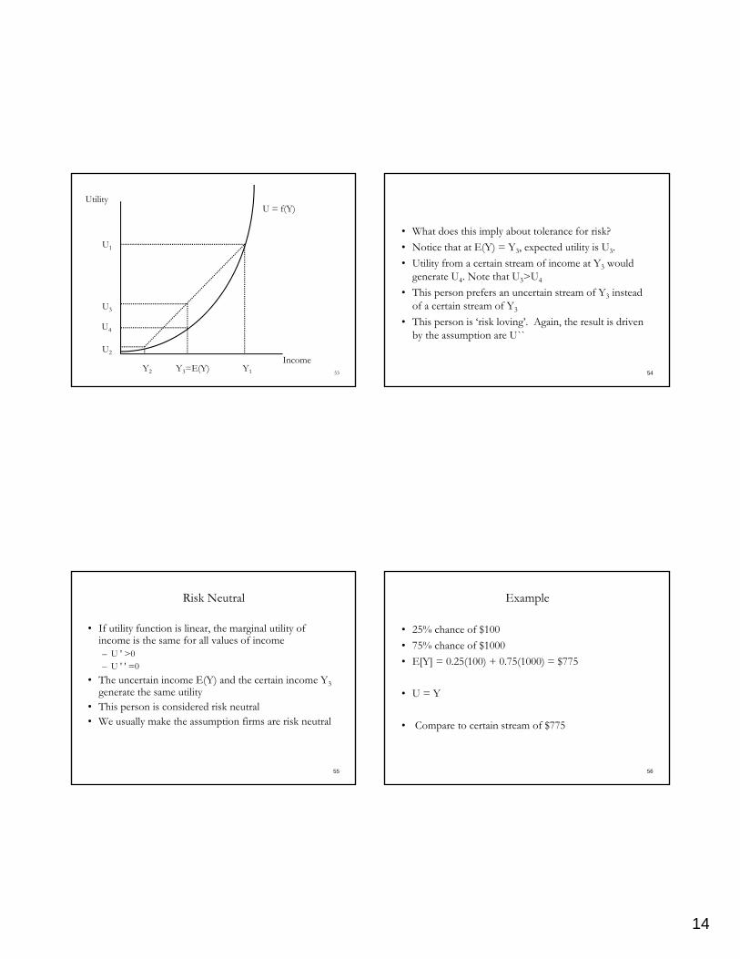
Risk Neutral

• If utility function is linear, the marginal utility of income is the same for all values of income– U ' >0– U ' ' =0

• The uncertain income E(Y) and the certain income Y3generate the same utility

• This person is considered risk neutral• We usually make the assumption firms are risk neutral

56

Example

• 25% chance of $100

• 75% chance of $1000

• E[Y] = 0.25(100) + 0.75(1000) = $775

• U = Y

• Compare to certain stream of $775

15

57

Utility

Income

U = a+bY

Y2 Y1Y3=E(y)

U2

U3 =U4

U1

58

Benefits of insurance

• Assume declining marginal utility

• Person dislikes risk– They are willing to receive lower certain income rather than

higher expected income

• Firms can capitalize on the dislike for risk by helping people shed risk via insurance

59

Simple insurance example

• Suppose income is know (Y1) but random --shocks can reduce income– House or car is damaged– Can pay $ to repair, return you to the normal state of world

• L is the loss if the bad event happens• Probability of loss is P1

• Expected utility without insurance is• E(U) = (1-P1)U(Y1) + P1U(Y1-L)

60

• Suppose you can buy insurance that costs you PREM. The insurance pay you to compensate for the loss L. – In good state, income is

• Y-Prem– In bad state, paid PREM, lose L but receive PAYMENT,

therefore, income is• Y-Prem-L+Payment

– For now, lets assume PAYMENT=L, so– Income in the bad state is also

• Y-Prem

16

61

• Notice that insurance has made income certain. You will always have income of Y-PREM

• What is the most this person will pay for insurance?• The expected loss is p1L• Expected income is E(Y)• The expected utility is U2

• People would always be willing to pay a premium that equaled the expected loss

62

• But they are also willing to pay a premium to shed risk (line cd)

• The maximum amount they are willing to pay is expected loss + risk premium

63

Utility

IncomeYY-L E(Y)Y2

cdU2

Willingness to pay forinsurance

64

• Suppose income is $50K, and there is a 5% chance of having a car accident that will generate $15,000 in loss

• Expected loss is .05(15K) = $750• U = ln(y)• Some properties of logs

Y=ln(x) then ey = exp(y) = xY=ln(xa) = a ln(x)Y=ln(xz) = ln(x) + ln(z)

17

65

• E(U) = P ln(Y-L) + (1-P)ln(Y)

• E(U) = 0.05 ln(35,000) + 0.95 ln(50,000)

• E(U) = 10.8

66

• What is the most someone will pay for insurance?• People would purchase insurance so long as utility with

certainty is at least 10.8 (expected utility without insurance)

• Ua =U(Y – Prem) ≥ 10.8• Ln(Y-PREM) ≥10.8• Y-PREM = exp(10.8)• PREM =Y-exp(10.8) = 50,000 – 49,021 =979

67

• Recall that the expected loss is $750 but this person is willing to pay more than the expected loss to avoid the risk

• Pay $750 (expected loss), plus the risk premium ($979-$750) = 229

68

Utility

Income$50,000$35,000 $49,021

cdU2

$49,250

$229

18

69

Supply of Insurance

• Suppose there are a lot of people with the same situation as in the previous slide

• Each of these people have a probability of loss P and when a loss occurs, they have L expenses

• A firm could collect money from as many people as possible in advance. If bad event happens, they pay back a specified amount.

70

• Firms are risk neutral, so they are interested in expected profits

• Expected profits = revenues – costs– Revenues are known

– Some of the costs are random (e.g., exactly how many claims you will pay)

71

• Think of the profits made on sales to one person

• A person buys a policy that will pay them q dollars (q≤L) back if the event occurs

• To buy this insurance, person will pay “a” dollars per dollar of coverage

• Cost per policy is fixed t

72

• Revenues = aq – a is the price per dollar of coverage

• Costs =pq +t– For every dollar of coverage (q) expect to pay this p percent

of time• E(π) = aq – pq – t• Let assume a perfectly competitive market, so in the long run π

=0• What should the firm charge per dollar of coverage? • E(π) = aq – pq – t = 0

19

73

• a = p + (t/q)• The cost per dollar of coverage is proportion to risk• t/q is the loading factor. Portion of price to cover

administrative costs• Make it simple, suppose t=0.

– a = p– If the probability of loss is 0.05, will change 5 cents per $1.00

of coverage

74

• In this situation, if a person buys a policy to insure L dollars, the ‘actuarially fair’ premium will be LP

• An actuarially fair premium is one where the premium equals the expected loss

• In the real world, no premiums are ‘actuarially fair’ because prices include administrative costs called ‘loading factors’

75

How much insurance will people purchase when prices are actuarially fair?

• With insurance– Pay a premium that is subtracted from income

– If bad state happens, lose L but get back the amount of insurance q

– They pay p+(t/q) per dollar of coverage. Have q dollars of coverage – so they to pay a premium of pq+t in total

• Utility in good state– U = U[Y – pq - t]

76

• Utility in bad state– U[Y- L + q – pq - t]

• E(u) = (1-p)U[Y – pq – t] + pU[Y-L+q-pq-t]

• Simplify, let t=0 (no loading costs)

• E(u) = (1-p)U[Y – pq] + pU[Y-L+q-pq]

• Maximize utility by picking optimal q

• dE(u)/dq = 0

20

77

• E(u) = (1-p)U[Y – pq] + pU[Y-L+q-pq]

• dE(u)/dq = (1-p) U'(y-pq)(-p) • + pU'(Y-L+q-pq)(1-p) = 0

• p(1-p)U'(Y-L+q-pq) = (1-p)pU'(Y-pq)

• (1-p)p cancel on each side

78

• U'(Y-L+q-pq) = U'(Y-pq)• Optimal insurance is one that sets marginal utilities in

the bad and good states equal• Y-L+q-pq = Y-pq• Y’s cancel, pq’s cancel, • q=L• If people can buy insurance that is ‘fair’ they will fully

insure loses.

79

Insurance w/ loading costs

• Insurance is not actuarially fair and insurance does have loading costs

• Can show (but more difficult) that with loading costs, people will now under-insure, that is, will insure for less than the loss L

• Intution? For every dollar of expected loss you cover, will cost more than a $1

• Only get back $1 in coverage if the bad state of the world happens

80

• Recall: – q is the amount of insurance purchased

– Without loading costs, cost per dollar of coverage is p

– Now, for simplicity, assume that price per dollar of coverage is pK where K>1 (loading costs)

• Buy q $ worth of coverage

• Pay qpK in premiums

21

81

• E(u) = (1-p)U[Y – pqk] + pU[Y-L+q-pqk]

• dE(u)/dq = (1-p) U' (y-pqk)(-pk)

• + pU'(Y-L+q-pqk)(1-pk) = 0

• p(1-pk)U'(Y-L+q-pqk) = (1-p)pkU'(Y-pqk)

• p cancel on each side

82

• (1-pk)U'(Y-L+q-pkq) = (1-p)kU' (Y-pkq)

• (a)(b) = (c)(d)

• Since k > 1, can show that

• (1-pk) < (1-p)k

• Since (a) < (c), must be the case that

• (b) > (d)

• U'(Y-L+q-pkq) > U'(Y-pkq)

• Since U'(y1) > U'(y2), must be that y1 < y2

83

• (Y-L+q-pqk) < (Y-pqk)

• Y and –pqk cancel

• -L + q < 0

• Which means that q < L

• When price is not ‘fair’ you will not fully insure

84

Demand for Insurance

• Both people have income of Y

• Each person has a potential health shock– The shock will leave person 1 w/ expenses of E1 and will

leave income at Y1=Y-E1

– The shock will leave person 2 w/ expenses of E2 and will leave income at Y2=Y-E2

• Suppose that– E1>E2, Y1<Y2

22

85

• Probabilities the health shock will occur are P1 and P2

• Expected Income of person 1– E(Y)1 = (1-P1)Y + P1*(Y-E1)

– E(Y)2 = (1-P2)Y + P2*(Y-E2)

– Suppose that E(Y)1 = E(Y)2 = Y3

86

• In this case– Shock 1 is a low probability/high cost shock

– Shock 2 is a high probability/low cost shock

• Example– Y=$60,000

– Shock 1 is 1% probability of $50,000 expense

– Shock 2 is a 50% chance of $1000 expense

– E(Y) = $59500

87Y1 Y2 YE(Y)=Y3Ya

Yb

a

b

c

Ua

Ub

d

fg

Utility

Income

U(Y)

88

• Expected utility locus– Line ab for person 1– Line ac for person 2

• Expected utility is – Ua in case 1– Ub in case 2

• Certainty premium –– Line (de) for person 1, Difference Y3 – Ya– Line (fg) for person 2, Difference Y3 - Yb

23

89

Implications

• Do not insure small risks/high probability events– If you know with certainty that a costs will happen, or, costs

are low when a bad event occurs, then do not insure

– Example: teeth cleanings. You know they happen twice a year, why pay the loading cost on an event that will happen?

90

• Insure catastrophic events– Large but rare risks

• As we will see, many of the insurance contracts we see do not fit these characteristics – they pay for small predictable expenses and leave exposed catastrophic events

91

Some adjustments to this model

• The model assumes that poor health has a monetary cost and that is all. – When experience a bad health shock, it costs you L to

recover and you are returned to new

• Many situations where – health shocks generate large expenses– And the expenses may not return you to normal– AIDS, stroke, diabetes, etc.

92

• In these cases, the health shock has fundamentally changed life.

• We can deal with this situation in the expected utility model with adjustment in the utility function

• “State dependent” utility– U(y) utility in healthy state

– V(y) utility in unhealthy state

24

93

• Typical assumption– U(Y) >V(Y)

• For any given income level, get higher utility in the healthy state

– U`(Y) > V`(Y)

• For any given income level, marginal utility of the next dollar is higher in the healthy state

94

Utility

Income

U(y)

Y2 YY1

ab

a

b

c

c

V(y)

95

Note that:

• At Y1, – U(Y1) > V(Y1)

– U`(Y1) > V`(Y1)

– Slope of line aa > slope of line bb

• Notice that slope line aa = slope of line cc– U`(Y1) = V`(Y2)

96

What does this do to optimal insurance

• E(u) = (1-p)U[Y – pq – t] + pV[Y-L+q-pq-t]

• Again, lets set t=0 to make things easy

• E(u) = (1-p)U[Y – pq] + pV[Y-L+q-pq]

• dE(u)/dq = (1-p)(-p)U`[Y-pq]

+p(1-p)V`[Y-l+q+pq] = 0

• U`[Y-pq] = V`[Y-l+q-pq]

25

97

• Just like in previous case, we equalize marginal utility across the good and bad states of the world

• Recall that – U`(y) > V`(y)– U`(y1) = V`(y2) if y1>y2

• Since U`[Y-pq] = V`[Y-l+q-pq]• In order to equalize marginal utilities of income, must

be the case that [Y-pq] > [Y-l+q+pq]

98

• Income in healthy state > income in unhealthy state

• Do not fully insure losses. Why?– With insurance, you take $ from the good state of the world

(where MU of income is high) and transfer $ to the bad state of the world (where MU is low)

– Do not want good money to chance bad

99

Allais Paradox

• Which gamble would you prefer– 1A: $1 million w/ certainty

– 1B: (.89, $1 million), (0.01, $0), (0.1, $5 million)

• Which gamble would you prefer– 2A: (0.89, $0), (0.11, $1 million)

– 2B: (0.9, $0), (0.10, $5 million)

100

• 1st gamble:• U(1) > 0.89U(1) + 0.01U(0) + 0.1U(5)• 0.11U(1) > 0.01U(0) + 0.1U(5)

• Now consider gamble 2• 0.9U(0) + 0.1U(5) > 0.89U(0) + 0.11U(1)• 0.01U(0) + 0.1U(5) > 0.11U(1)

• Choice of Lottery 1A and 2B is inconsistent with expected utility theory