1

Intermittent Reinforcement and the Persistence of Behavior:

Experimental Evidence

Robin M. Hogarth and Marie Claire Villeval

June 26, 2010

Abstract: Whereas economists have made extensive studies of the impact of levels of incentives on behavior, they have paid little attention to the effects of regularity and frequency of incentives. We contrasted three ways of rewarding participants in a real-effort experiment in which individuals decided when to exit the situation: continuously (all periods paid); a fixed intermittent reinforcement schedule (one out of three periods paid); and a random intermittent reinforcement schedule (one out of three periods paid on a random basis). In all treatments, monetary rewards were withdrawn after the same unknown number of periods. Overall, intermittent reinforcement leads to more persistence and higher total effort, while participants in the continuous condition exit as soon as payment stops or decrease effort dramatically. Randomness increases the dispersion of effort, inducing both early exiting and persistence in behavior; overall, it reduces agents’ payoffs. One interpretation is that both the continuity and the randomness of the reinforcement schedules influence adjustments that participants make across time to their reference points in earnings expectations. We discuss implications for cross-temporal economic phenomena subject to regime shifts.

Keywords: Intermittent reinforcement, ambiguity, randomness, incentives, experiment JEL Classifications: C92, M54, J28, J31

Contact: Robin M. Hogarth, ICREA, Department of Economics and Business, Universitat Pompeu Fabra, Ramon Trias Fargas, 25–27, 08005 Barcelona, Spain. E-mail: robin.hogarth@upf.edu Marie Claire Villeval, University of Lyon, F-69007; CNRS-GATE, 93 Chemin des Mouilles, F-69130, Ecully, France; IZA, Bonn, Germany; CCP, Aarhus, Denmark. E-mail: villeval@gate.cnrs.fr Acknowledgments: The authors are grateful for comments from Donald A. Hantula, Karl Schlag and seminar participants at Universitat Pompeu Fabra. They also thank Romain Zeiliger for programming the experiment. Financial support from the Agence Nationale de la Recherche (ANR BLAN07-3_185547 “EMIR” project) is gratefully acknowledged.

2

1. INTRODUCTION

In an intriguing paper, Odean (1999) asked: “Do investors trade too much?” His answer,

based on studying trading in equity markets by investors with discount brokerage accounts

was positive. Investors, one might assume, were overconfident? Perhaps, but it seems that

some other factor was involved because the “result is more extreme than… predicted by

overconfidence alone” (Odean, 1999, p. 1296).

The purpose of this paper is to draw attention to a possible behavioral explanation for why

economic actors persist in activities that continue to lead to no gains or even losses. In

addition to stock trading, these can include, for example, persisting in unprofitable

investments in R & D or marketing efforts, banks extending additional credit to customers

with financial difficulties, or even some forms of gambling behavior. The situations that

concern us are characterized by two structural features: first, they involve repeated activities

across time; and second, there are one or more temporal regime shifts, i.e., where the

probabilities of the underlying system generating outcomes change. For example, the

probability that a bank’s customer is able to repay loans suddenly becomes lower.

When agents engage in repeated activities across time, economists typically assume that

learning results from feedback and opinions are updated in a Bayesian manner. However,

there is little or no theoretical concern that the structure as opposed to the informational

content of feedback might have effects. Indeed, there is not even much awareness of this

issue (for exceptions, see Lazear, 1990; 1991; O’Flaherty & Komaki, 1992; Eriksson et al.,

2009). In psychology, however, the effects of different types of feedback – or so-called

reinforcement schedules – have been studied extensively for decades (see, e.g., Ferster &

Skinner, 1957).

3

Although there are many possible reinforcement schedules, it is useful to distinguish between

two general types: continuous and intermittent (see, e.g., Hilgard and Bower, 1975). To

illustrate, imagine a worker who is producing a series of widgets across time. With a

continuous reinforcement schedule, the worker is rewarded for each trial (i.e., widget or batch

of widgets) successfully completed.1 If, on the other hand, the worker is only rewarded

periodically (say, once, in three trials), the reinforcement schedule is intermittent. Moreover,

this can be variable or fixed in nature. Variable means that trials are rewarded on a varying or

random basis; fixed means that they are rewarded on a regular basis (e.g., every 3rd trial).

Much research has examined the effects of learning by both humans and animals (notably rats

and pigeons) under different reinforcement schedules. Of particular interest to the economic

phenomena described above is what happens when there is a change in schedule, particularly

when no further rewards are given (in a so-called extinction phase). The main result

distinguishes situations where prior learning was reinforced by continuous as opposed to

intermittent schedules. Given the former, the organism ceases the previously reinforced

activity almost immediately, i.e., there is extinction of the learned response. Given the latter,

the organism persists in the activity that is no longer rewarded for some time, and particularly

if learning has taken place under variable intermittent reinforcement. Indeed, Hilgard and

Bower (1975) state “Responses trained on VI schedules are ….unusually resistant to

extinction; it is not unusual, for instance, to observe pigeons responding more than 10,000

times during extinction following VI training. Resistance to extinction depends roughly on

the mean and maximum interval in the VI program” (Hilgard & Bower, 1975, p. 215).

It’s not hard to make the link with different forms of economic activity. For most workers,

monthly paychecks provide a form of continuous reinforcement and bonuses are experienced

as intermittent. The thought of a possible bonus can be very motivating. For investment

1 Of course, the schedule where no trial ever gets rewarded is also “continuous.”

4

bankers, on the other hand, annual bonuses provide continuous reinforcement such that the

failure to pay them can trigger exits. Trading in the stock market is also subject to variable

intermittent reinforcement and many people clearly persist in the face of failure.

This paper investigates possible differential effects of continuous and intermittent

reinforcement schedules in an economic context. Participants in a laboratory experiment were

required to perform a task repeatedly and to decide when to exit the situation. As such, goal

setting was endogenous (see Locke & Latham, 1990, for a review of goal setting in

psychology). We compare three treatments in a between-subjects design. In the baseline

treatment, participants were paid a piece-rate and each period gave rise to actual payment.

This corresponds to a continuous reinforcement schedule. In the random intermittent

reinforcement treatment, on average one period out of three was paid and the sequence of

payments was random for each participant. In the fixed intermittent reinforcement treatment,

one period out of three was paid according to a fixed schedule. In all three treatments, the

20th period was paid but payment stopped thereafter. The participants were informed of the

amount of the piece-rate but they received no ex ante information about the sequences of

payments. They were only informed at the beginning of the session that some periods would

be paid whereas others would not, and at the end of each period, whether it was paid or not.

The environment we created in the laboratory is highly ambiguous and, since this could in

itself affect decisions, we also elicited participants’ risk attitude and ambiguity aversion.

Our main findings indicate that in the baseline treatment participants generally exit soon after

payment stops. On the other hand, participants in the random intermittent reinforcement

treatment exit either before or long after payment stops, with the fixed intermittent

reinforcement treatment in an intermediate position. Moreover, in the continuous

reinforcement treatment, once payment stops individuals who do not exit immediately exert

significantly lower effort than those under the other reinforcement schedules. Overall,

5

intermittent reinforcement leads to more persistent behavior, higher average effort levels, but

lower payoffs for agents. This variation of effort across treatments after rewards cannot be

rationalized by theories of income targeting (Camerer et al., 1997). We also find that risk

aversion increases significantly the likelihood of early exit while, controlling for risk attitude,

ambiguity aversion reduces it.

The remainder of the paper is organized as follows. Section 2 summarizes briefly the related

literature in economics and psychology. Section 3 describes the experimental design and

experimental protocol. Section 4 presents the results of the study and section 5 contains our

concluding remarks.

2. RELATED LITERATURE

Given the potential ubiquity of variable reinforcement schedules in economic life, it is

surprising that economists have not been more concerned with their implications. Somewhat

related to our analysis, some economic studies have investigated how affect and cognition

influence the allocation of effort in reaction to changing incentives over time. However, this

change is usually a variation in the level of compensation (see, e.g., Fehr and Goette, 2007),

not in its structure. For example, Camerer et al. (1997) have used income targeting by

cabdrivers to explain the negative response of hours worked to an increase in daily wages.

Other studies have suggested that variations of motivation within a workday could explain

this negative correlation (Goette et al., 2004). Goette and Huffman (2006) argue that the

affective system reacts to within-day variations in earnings relative to an income target but

once this is reached, the affective system does not react to earnings anymore. Based on a

model of reference-dependent preferences with endogenous reference point determination

based on expectations, Koszegi and Rabin (2006) explain that workers are likely to stop

working if the income earned thus far is unexpectedly high but will continue to work if

expected income is high. Whereas these analyses can potentially explain that individuals

6

sometimes persist in efforts when incentives are removed (if expectations of earnings remain

unaffected), they do not consider the influence of various continuous/intermittent

reinforcement schedules on the endogenous determination of the reference point, and thus on

the allocation of effort.

On the other hand, several investigations of variable reinforcement schedules have been

conducted in applied psychology. For example, in a field study, Deslauriers and Everett

(1977) showed how, to increase bus ridership, it was more effective to offer passengers

variable as opposed to continuous reinforcement (gifting tokens worth 10 cents to roughly

every one in three passengers versus every passenger receiving a token). Golz (1992)

pioneered an experimental investment game in which groups of participants could earn or lose

money by investing under different reinforcement conditions (continuous and variable).

There were two phases in the experiment – acquisition and extinction. In the first, the market

allowed participants to be successful; in the second, it did not. The main result was that

participants exposed to continuous reinforcement in the acquisition phase invested much less

in the failing extinction phase than those who experienced the variable reinforcement

condition in the acquisition phase.

Golz’s paradigm has been replicated and extended in a series of studies by Hantula and his

colleagues (Hantula and Crowell, 1994; DeNicolis Bragger et al., 1998, 2003; Hantula and

DeNicolis Bragger, 1999; Brecher and Hantula, 2005). At an experimental level, the

extensions involved different types of decision/investment scenarios, differential levels of

uncertainty in feedback (i.e., low versus high variance of returns as feedback), and different

measures of decisions (information purchased, time to exit decisions, as well as amounts

invested).2 All results, however, are consistent with the notion that variable reinforcement

2 In clinical settings, psychologists have also studied whether intermittent vs. continuous schedules of reinforcement might increase the resistance of patients’ problem behavior to extinction. See for example Lerman et al. (1996).

7

schedules induce responses that are more immune to extinction than their continuous

counterparts.

On the other hand, by making different reinforcement schedules operational through returns

having low and high variance (i.e., substituting for continuous as opposed variable schedules),

Hantula and his colleagues opened the door to a further interpretation of persistence of

behavior in the second phases of their experiments. Since feedback in their experiments was

not unequivocal (differing only between conditions on variance), it could be argued that, by

investing more or delaying exit longer, participants were in fact dealing rationally with the

uncertainties they faced. Indeed, this view has been argued by Bowen (1987) in the

management literature and is consistent with the observations of Dixit (1992) in economics.

Bowen (1987) suggests that situations involving persistence should be viewed as decision

dilemmas that managers handle by dealing with the uncertainties in the situations as they

perceive them ex ante. It is not clear, therefore, that sticking to a particular commitment

results from decision making errors. If there is an error, it is usually that of third parties

judging decisions ex post. Dixit (1992) presents an economic analysis of situations where

there might be a change in underlying circumstances. In addition to failures to exit particular

activities, he considers failures to invest. As he states, there might be “a theory of optimal

inertia” where “firms that refuse to invest even when the currently available rates of return are

far in excess of the cost of capital may be optimally waiting to be surer that this state of

affairs is not transitory. Likewise, farmers who carry large losses may be rationally keeping

their operation alive on the chance that the future may be brighter” (Dixit, 1992, p. 109).

There is a closely related literature on so-called escalation processes. These consider

situations where an investment that went sour is nonetheless pursued and involves more

losses across time (Staw, 1976; Staw and Ross, 1989). This research has seen much activity

in management and social psychology and has involved both cases studies and numerous

8

experiments where participants are asked to imagine themselves taking decisions in specific

scenarios. Whereas some explanations point to cognitive errors such as the failure to

understand sunk costs, others are motivational in nature and emphasize the realpolitik of

organizational life. Thus, for example, Brockner (1992) has argued that, by continuing to

invest in losing projects, people are often engaging in a process of self-justification.

In this paper, it is not our intention to adjudicate between cognitive or motivational

explanations of continuous versus intermittent reinforcement schedules. Instead, we examine

this phenomenon within a straightforward, economic context. We say “straightforward”

because we wish to abstract from the myriad of possible organizational considerations; we say

“economic” because none of the experimental evidence referred to above involved

participants who faced proper incentives. In addition, the tasks they faced required relatively

little effort.3

3. EXPERIMENTAL DESIGN

3.1. Experimental treatments

Our experiment consists of three different treatments and is based on a between-subjects

design. In our baseline treatment, each participant has to perform a task that consists of

counting the occurrence of four different letters in a paragraph. This task is repeated in

different periods across time. In each period, a different paragraph is displayed on the

participant’s screen during two minutes. The paragraph consists of meaningful words that are

randomly combined to form four meaningless sentences. The letters to be counted appear

successively. All the participants receive the same paragraphs and the same letters in the

same order. The difficulty of the task is comparable across periods although the total number

of words and letters in each line may differ since they are randomly displayed. An answer is

3 We are, of course, fully aware that if an experiment does not involve properly incentivized participants, it does not mean that its conclusions are necessarily invalid (Camerer and Hogarth, 1999).

9

considered correct if it corresponds to the true value plus or minus one. The participants are

informed if a submitted answer is correct or not and the next letter is displayed. They are also

continuously informed of the current number of their correct answers.

Participants are informed that they have to complete a minimum of 15 periods after which

they are free to exit the situation. There is a maximum of 35 periods (i.e., 70 minutes) but this

is not made common information. In other words, the participants can exit voluntarily

between the 16th and the 35th periods. Participants are also informed that not all periods are

paid but they do not know in advance whether a period will be paid or not. Nor are they

informed about the total number of paying periods. At the end of each period, they are

informed ex post whether correct answers provided in that period are or are not paid.

In the baseline treatment, all correct answers given in each of the first 20 periods are rewarded

monetarily at the end of the session (i.e., when the participants have completed all

experimental tasks). After the 20th period, however, the correct answers no longer give rise to

paying points. When periods are paid, each correct answer is rewarded with one paying point,

such that between 0 and 4 points can be earned in a period. There is no penalty for providing

wrong answers. It is also made common information that as soon as the participant decides to

start a new period, he or she has to pay an entry fee of 1 point. This entry fee has to be paid

whether correct answers are or are not paid in the period. Therefore, whereas payment of the

entry fee is certain, the reward is uncertain.

To summarize, although participants have to enter the first fifteen periods of the task, this

changes at the beginning of the sixteenth period. Now, before the beginning of a period, the

participant must decide whether to start the period or not. If he or she starts the period, a new

paragraph is displayed on the participant’s screen during two minutes and four letters appear

successively. Once the two minutes have elapsed, the participant is informed whether the

period gives rise to payment or not. The screen also displays the total number of accumulated

10

paying points. If the participant decides not to start a new period, he or she has to confirm

this decision and exit the task.

The fixed intermittent reinforcement treatment is identical to the baseline treatment except

that during the first 20 periods, one period out of three is paid (i.e., the 2nd, 5th, 8th, 11th, 14th,

17th, and the 20th periods). In addition, in the paid periods each correct answer is rewarded by

three paying points instead of one in the baseline treatment.4 Here too, no payment is made

after the 20th period.

The random intermittent reinforcement treatment is identical to the fixed intermittent

reinforcement treatment (in particular, one period out of three is paid during the first 20

periods), except that the sequence of paid periods in the first 20 periods is randomly generated

for each participant. Although sequences differ across participants, to facilitate comparisons

between treatments, we impose the constraint that correct answers are paid for the 20th period.

As before, no more payment occurs after period 20. As in the fixed intermittent

reinforcement treatment, correct answers are paid three times more than in the baseline

treatment. In the three treatments, the same paragraphs appear in the same order to guarantee

that the difficulty of the task is kept constant across treatments.

Comparing the baseline and the fixed intermittent reinforcement treatments helps to identify

the impact of the frequency of rewards on exiting decisions, payoffs, and effort. Comparing

the random intermittent reinforcement treatment with the two other treatments allows us to

measure the impact of the randomness of rewards.

4 In the baseline treatment, participants can earn a maximum of 80 paying points in the session (4 correct answers*1 point*20 paying periods), while in the two other treatments, the maximum is slightly higher, i.e., 84 (4 correct answers*3 points *7 paying periods). Therefore, the incentive to exert effort may be slightly higher in the intermittent reinforcement schedules. To make treatments identical on this point, we could have used a piece- rate of 2.86 instead of 3 in the intermittent reinforcement treatments. We reasoned, however, that this piece-rate would not be easily interpreted by the participants. In addition, since participants did not know in advance the sequence of payments, we do not believe that the difference we indicate has affected behavior.

11

At the beginning of each experimental session, we elicit – for all treatments – participants’

attitudes toward risk and uncertainty by asking them to price both a clear and a vague bet

following a procedure similar to that of Fox and Tversky (1995) (see instructions in Appendix

A). The participants have to make a first set of 20 decisions between accepting a certain

payoff and drawing a ball in an urn that contains 5 blue balls and 5 yellow balls (a risky

lottery). The amount of the certain payoff increases from 0.25 Eurocents to 5 Euros. One

yellow ball drawn from the urn pays € 5, a blue ball pays nothing. Then, the participant has to

make a second set of 20 similar decisions except that the proportions of yellow and blue balls

in the urn are now unknown (an ambiguous lottery). In both sets of decisions, a risk neutral

participant should choose to draw a ball from the urn until the certain payoff is equal to at

least € 2.5. In the first set, a risk averse participant should switch from the lottery to the

certain payoff for certain payoffs lower than € 2.5 and a risk seeking participant should switch

for certain payoffs higher than € 2.5. An ambiguity averse (seeking) participant should switch

from the lottery to the certain payoff for lower (higher) certain amounts in the second set of

decisions (the ambiguous lottery) than in the first set (the risky lottery). Decisions are made

at the beginning of the session and participants are told that the outcome of these decisions

will be determined only at the very end of the session once all other experimental tasks have

been completed. When making their decisions, participants are also informed that one of the

two sets of decisions will be randomly drawn for real payoffs at the end of the session.

In all treatments, when participants decide not to start a new period or when the final period

has been reached, they have to answer questions as to why they did or did not decide to exit.

A demographic questionnaire follows.

3.2. A Bayesian model of reinforcement

Given that participants do not know the probabilities that periods will or will not be paid, nor

that this probability can change at any time, one should ask what is appropriate for them to

12

reason a priori. One obvious rational candidate is a Bayesian model in which participants

update their estimates of the probability that a particular period will be paid given the past

history of payments experienced up to that point.5 However, this model requires different

assumptions that may or may not be appropriate.

In Appendix B, we present implications of different Bayesian models for the baseline and

fixed intermittent reinforcement treatment, respectively. Taking all data into account, these

models predict that participants should continue in the sessions through period 35 even

though the probability of payment starts decreasing after period 20. However, if the Bayesian

model is based on limited memory (i.e., only the k last observations), exiting before period 35

is seen to be rational for specific values of k.

3.3. Experimental procedures

The experiment consisted of 12 sessions conducted at the laboratory of the GATE (Groupe

d’Analyse et de Théorie Economique) research institute in Lyon, France. Between 12 and 19

individuals took part in each session, for a total of 210 participants invited via the ORSEE

software (Greiner, 2004). No individual participated in more than one session. The

participants were mostly undergraduate students from the local engineering and business

schools. In each treatment, half of the sessions were run at 12 noon and half were run at 2pm,

to control for the possibility that exiting decisions could be influenced by differing

opportunity costs of time during the day. Table 1 displays summary information about the

5 Of course, if participants knew a priori that no payments would be made after some unspecified period, a Bayesian model could be formulated to calculate the odds of sampling from one process or another (see, e.g., Kacelnik et al., 1987; Massey and Wu, 2005). However, since our participants were not aware that there would be such a change, we are not convinced that this would provide a reasonable normative benchmark.

13

sessions. It states the session number, number of participants, percentage of male participants

per session, and the treatment.6

(Insert Table 1 about here)

Five participants were invited in a session every quarter of an hour. Upon arrival, a

participant was directly sent to the laboratory and was randomly assigned to a computer

terminal by drawing a tag from a bag. Therefore, when entering the laboratory most

participants found others already working at the task. This procedure aimed at making it

impossible for anybody to know how much time other participants had been in the laboratory.

Indeed, the moment when a participant left the laboratory was not informative as to the period

when he or she exited the task.

The participants found the instructions for both the risky and ambiguous lotteries in their

cubicle (see Appendix A). They raised a hand if they had questions. Questions were

answered in private. Then, after the decisions were completed, the experimenter took back

the instructions and decision sheets for the elicitation tasks and distributed the instructions for

the main task. Again, questions were answered in private. When ready, participants could

start by playing two practice periods on the computer to familiarize themselves with the task.

Except for the elicitation of attitudes toward risk and ambiguity that used pen and paper, the

experiment was computerized, using the REGATE platform (Zeiliger, 2000).

After completion of the final demographic questionnaire, the participants were informed on

their screens that they were allowed to leave the room, they should not speak to anyone and

proceed to the payment room. There, each participant was first asked to flip a coin to

determine which set of decisions would be played for real. Then, he or she drew a tag from a

6 We ran five sessions of the baseline treatment and five sessions of the random intermittent reinforcement treatment but only two sessions of the fixed intermittent reinforcement treatment (with 36 independent observations). This was because we considered the latter to be more of an intermediate treatment. In fact, it turned out that the treatment effects were so strong that we did not deem it necessary to have more observations.

14

box to determine which of the 20 decisions would be considered. If for this decision, the

participant had chosen the certain payoff at the beginning of the session, this amount was

added to his or her other earnings. If the lottery was chosen, the participant drew a ball from

either from a transparent bag (the risky lottery) or from a dark bag (the ambiguous lottery). If

the ball was yellow, € 5 were added to the other earnings and € 0 otherwise. Then, the

participant could leave the building.

The experiment lasted on average 70 minutes, including the payment of participants, and each

participant earned an average of € 14.29 (standard deviation € 2.81), including a show-up fee

of € 4 and the payoff from either the risky or the ambiguous lotteries.

4. RESULTS

4.1 Descriptive statistics

The main questions of interest focus on the performance across trials of the participants in the

three treatment groups, specifically: (1) When do they exit the experimental task? (2) How do

they perform? (3) How much do they earn?

Exiting time patterns

Figures 1 and 2 speak to the first question. To interpret these figures, recall that period 15

ends the compulsory stage and that payment is stopped after period 20. Figure 1 shows when

participants in the three treatment groups exit the task (from the end of periods 15 to 35).

Figure 2 complements this by displaying the percentages of participants in the three treatment

groups who had not exited the task after the 15th, 20th, 25th, 30th, and 35th periods.

(Insert Figures 1 and 2 about here)

Both figures reveal that the distributions of exiting behavior are quite different across

treatments. In the baseline, the distribution is approximately symmetrical with a median (and

mode) of 17% at the 22nd period (see Fig.1). Compared to the intermittent reinforcement

15

treatments, few participants in the baseline treatment exit the task when it continues to be paid

but is no longer compulsory. However, the effect of stopping payment is dramatic (see

Fig.2). By the end of period 25, only 29% of baseline participants remain in the task. At the

end of the task (period 35, when participants were required to stop), only 2% remain.

The distribution of exiting periods is strikingly different in the random intermittent

reinforcement (random IR) treatment. Most importantly, the mode of the distribution

corresponds to period 35 in which 20% of the participants have to be forced to stop (see

Fig.1). In addition, 36% of the participants in the random IR treatment exit between periods

15 and 20, i.e., before payment stops, while the corresponding percentages are 20% in the

baseline and 25% in the fixed intermittent reinforcement (fixed IR) treatment. The exiting

behavior of the remaining individuals looks like a random pattern. Compared with the other

treatments, randomness of reinforcement is associated with a less steep decline in the number

of participants remaining over time (see Fig.2).

The pattern of the fixed IR treatment is relatively close to that of the random IR treatment, but

there are some differences. The fixed IR treatment has an apparent tri-modal distribution:

11% of the participants exit at period 15, 17% at period 26, and 8% at each of the 33rd, 34th,

and 35th periods (see Fig.1). Participants in the IR-fixed treatment are somewhat slower to

exit the task than those in the IR-random treatment before period 25, but after this the rate of

exiting increases and only 8% remain after period 35 (see Fig.2).

Kolmogorov-Smirnov tests (K-S hereafter) confirm that the distribution of exiting periods is

significantly different between the baseline and both the random IR treatment (p<0.001,

exact) and the fixed IR treatment (p<0.001, exact). However, the distributions of the two

intermittent reinforcement treatments are not significantly different (p = 0.222, exact). Mann-

Whitney tests (at the mean values; M-W hereafter) show qualitatively similar results. The

average exiting period is lower in the baseline than in both the random IR treatment (p =

16

0.052) and the fixed IR treatment (p = 0.002) but there is no difference between the two IR

treatments (p = 0.693).7

Performance profiles

Figure 3 displays the evolution of the participants’ number of correct answers per period over

time in each treatment. Table 2 summarizes the means and standard deviations of four sets of

performance measures and the amounts participants received for their task performance. The

first set of measures indicates the number of correct answers by blocks of periods. The

second set shows the number of correct answers for periods 1 to 20 conditional on whether

the previous period (or the previous two periods) gave rise to payment or not; in periods 22 to

35, the previous period is always unpaid. This set of measures captures whether participants

adjust their effort to any regular pattern in payments; i.e., in the fixed IR treatment do they

anticipate that the period that follows two unpaid periods will be paid? The third measure

indicates the total number of correct answers per treatment. The fourth measure corresponds

to the total number of paying points (i.e., net of entry fees) actually earned by the participants

by the end of the session.8 To make comparisons with the baseline treatment, we have

divided this number of paying points by 3 in the two IR treatments.

(Insert Figure 3 and Table 2 about here)

Both Figure 3 and measures 1 in Table 2 indicate that there is hardly any difference in

performance per period between treatments in the first 20 periods. K-S tests confirm that

7 We note that due to the specific distributions of exiting periods across treatments, a simple comparison of mean exiting periods would be quite misleading. The means (standard deviations) for the three treatments (baseline, random IR, fixed IR, respectively) are: 23.18 (4.00), 25.48 (7.17), and 26.44 (6.90). 8 Figure 3 and measures 1, 2 and 3 have been computed with the data from the last six sessions (two per treatment), with N=35 in the baseline treatment, N=35 in the random IR treatment, and N=36 in the fixed IR treatment. Measure 4 has been computed with the data from the 12 sessions (N=89 in the baseline treatment, N=85 in the random IR treatment, and N=36 in the fixed IR treatment). The reason is that, by mistake, the number of correct answers was recorded only in the paid periods in the first six sessions (three with the baseline and three with the random IR treatments). Therefore, we do not use these sessions for the calculation of the first four measures. Figure 3 is also based on the data of the last six sessions. We note, however, that the distribution of exiting periods by treatment is the same in the first six and the last six sessions (K-S test, p=0.398 for the baseline and p=0.937 for the random IR treatment).

17

there is no significant difference in the distribution of the number of correct answers in the

first 20 periods between the baseline and the random IR treatments (p = 0.492), between the

baseline and the fixed IR treatment (p = 0.532), and between the two IR treatments (p =

0.611). In contrast, once payment stops definitively the average performance in the baseline

treatment decreases rapidly whereas effort remains high in both IR treatments. K-S tests

show that the distribution of the number of correct answers after period 20 is significantly

different between the baseline and the random IR treatment (p<0.001), between the baseline

and the fixed IR treatment (p = 0.001), but not between the two IR treatments (p = 0.995).9

This suggests that participants who do not exit early in the baseline treatment have little

motivation but stay just in case payment might restart. In the IR treatments, performance

increases slightly throughout the game, due possibly to a combination of learning and self-

selection by the most able participants over time.

Figure 3 also indicates that performance fluctuates across periods in each treatment but no

regular pattern emerges. In particular, measures 2 in Table 2 suggest that in the fixed IR

treatment participants do not learn and anticipate that in the first 20 periods a period is always

paid after two unpaid periods. Indeed, in this treatment performance in the first 20 periods is

not higher after two periods unpaid than after one unpaid period (Wilcoxon test, p = 0.642; for

the random IR treatment, p = 0.646). Similarly, performance does not decline after one

period has been paid (Wilcoxon test, p = 0.712). Fluctuations between two periods are more

likely due to variations in task difficulty (i.e., the number of occurrences of the four letters in

the sentences).

9 Mann-Whitney tests on the number of correct answers by blocks of periods reach the same conclusions. For periods 1 to 20, the p-value is 0.819 for the comparison between the baseline and the random IR treatment, 0.617 for the comparison between the baseline and the fixed IR treatment, and 0.774 for the comparison between the two IR treatments. For periods 21 to 25, the p-values are 0.084, 0.290 and 0.418, respectively. For periods 26 to 30, they are 0.016, 0.009, and 0.966. Last, for periods 31 to 35, they are 0.031, 0.097, and 0.550.

18

Last, measures 3 in Table 2 indicate that the total performance is lower in the baseline (mean

= 66.91 correct answers) than in the random IR treatment (mean = 80.83, M-W test: p =

0.069) and the fixed IR treatment (mean = 84.28, p = 0.003), with no difference between the

last two treatments (p = 0.709). This results from the longer participation of players in the IR

treatments.

Average payoffs

Consider now the net amount of paying points earned by the participants in the 12 sessions.

Measures 4 in Table 2 show that the participants who are still involved in period 20

accumulated more points in the first 20 periods in the random IR treatment (mean = 47.37)

than in the baseline (mean = 42.01; M-W test, p = 0.001) and than in the fixed IR treatment

(mean = 41.89; p = 0.028). There is no difference between the baseline and the fixed IR

treatments (p = 0.955). This higher number of points earned in the random IR treatment is

probably due to the early exiting of less able participants (see the econometric analysis

below). If one considers instead the final number of paying points earned by all the

participants, we find that this number is slightly higher in the baseline (mean = 37.31) than in

both the random IR treatment (mean = 35.65; M-W test, p = 0.113) and the fixed IR treatment

(mean = 33.39; p = 0.051). These differences between points earned until period 20 and

points earned throughout the sessions across treatments are clearly due to the fact that

participants played in more unpaid periods in the IR treatments than in the baseline. There is

no difference between the two IR treatments (p = 0.319).

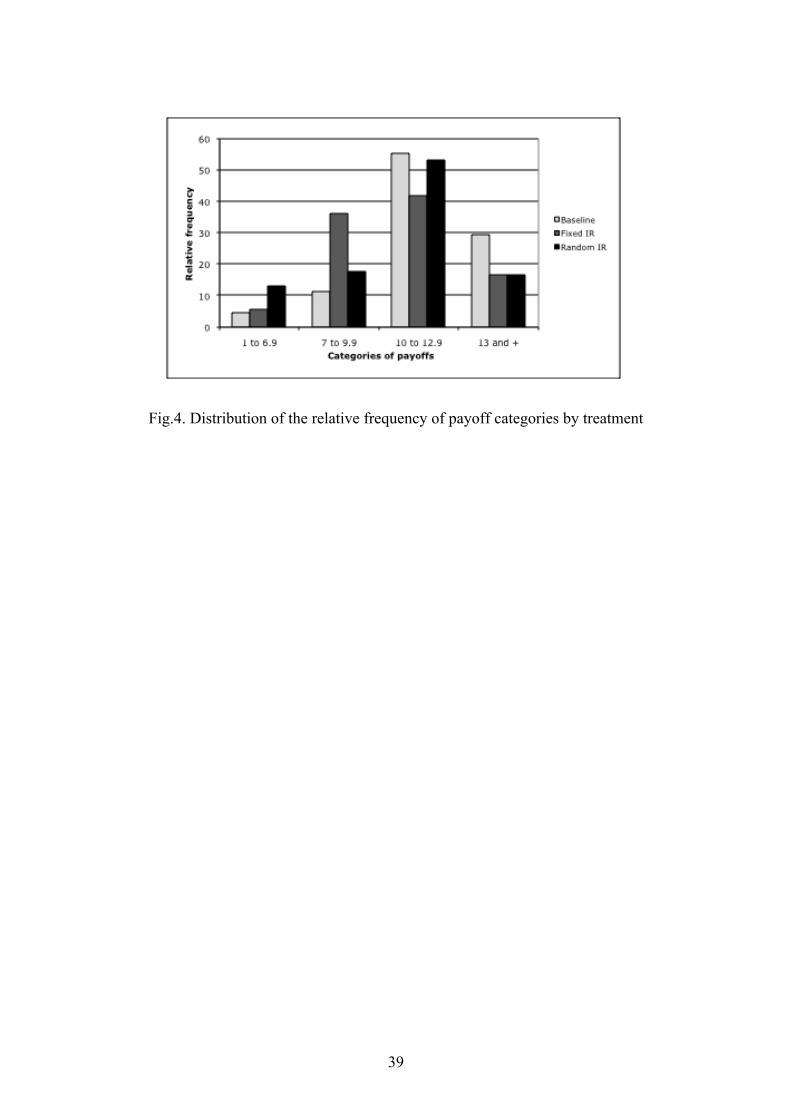
Figure 4 complements this analysis by displaying the distribution of monetary payoffs by

experimental treatment.

(Insert Figure 4 about here)

19

Figure 4 shows that the baseline treatment is associated with higher payoffs than the

intermittent reinforcement treatments, while the fixed IR treatment is associated with lower

payoffs. Participants in the baseline treatment clearly adapted better to changing

circumstances than those in the IR conditions.

Could these differences between treatments in exiting period, performance, and payoffs be

attributed to differences in individual characteristics of the participants in each treatment? To

address this question we investigated possible differences between the three treatments in

terms of skill at the task as measured by the distribution and the means of correct answers in

the two practice rounds as well as the first 15 compulsory periods. None of these differences

were significant, although the average score during the practice period was marginally higher

in the random IR than the baseline treatment (p = 0.079).10 We also found no significant

differences in switch point in the ambiguous lottery nor any ambiguity aversion defined as the

difference between switch points of the risky and ambiguous lotteries.11 Observed differences

in exiting periods and effort can thus be imputed to the treatment manipulation and not to

different characteristics of the participants across treatments.

4.2 Econometric analyses

To complement this analysis we carried out some econometric tests. More precisely, we

estimated a tobit model in which the dependent variable is the period at the end of which the

participant decided to exit the session. We estimate a tobit model because data are censored

10 In the following, the three p-values correspond always to the comparison between the baseline and the random IR treatment, then between the baseline and the fixed IR treatment, and last between the random and the fixed IR treatments. Regarding the score in practice periods, K-S tests indicate p=0.270, 0.269, and 0.800, while M-W tests yield p=0.079, 0.213, and 0.784. Regarding the cumulated score at the end of period 15, K-S tests indicate p=1.000, 0.975, and 0.818, while M-W tests yield p=0.934, 0.904, and 0.977. Last, considering the cumulated number of mistakes during the 15 periods of the compulsory task, K-S tests indicate p=0.999, 0.785, and 0.594, while M-W tests yield p=0.724, 0.890, and 0.738. 11 With the same convention as in the previous footnote, K-S tests yield p=0.923, 0.871, and 0.863 for the switching point for the ambiguous lottery, and p=0.710, 0.998, and 0.548 for ambiguity aversion.

20

both on the left (participants are not allowed to exit before the end of the 15th period) and on

the right (they cannot start a 36th period).

The independent variables include two dummy variables for the random IR treatment and the

fixed IR treatment, with the baseline treatment as the omitted reference category. They also

include a dummy variable for the afternoon sessions since participants may have a higher

opportunity cost for staying longer in the afternoon than during the lunch break. The rank of

arrival variable aims at capturing the impact on the participant’s exiting decision of observing

other participants leaving. For example, participants who arrive late might decide to exit

earlier simply because they see their peers leaving the laboratory before them.12

The other variables capture individual characteristics. The skill variable takes the value of the

number of correct answers provided by the participant in the 15 compulsory periods.13 We

hypothesize that participants who are less able at the task may leave earlier than the more

able. We include three variables for capturing the attitudes of participants towards risk and

ambiguity. The risk index indicates the number of the decision where the participant

switched from the lottery to the certain equivalent. The higher (lower) the value of the

variable, the less (more) risk averse the participant, since this indicates valuing the lottery

more (less). The ambiguity aversion variable expresses the difference between the value of

the switching point in the risky lottery and the value of the switching point in the ambiguous

lottery. This variable can take positive or negative values. A positive (negative) value means

that the participant has switched from the random drawing to the certain equivalent earlier

(later) for the ambiguous lottery than for the risky lottery, thereby indicating some ambiguity

aversion. Since 22 out of 210 participants (10.5%) switched several times (in 21 cases for

12 The rank of arrival is a better instrument to capture peer effects in exiting than the rank of departure because the former is exogenous while the latter is endogenous to the exiting decision. 13 We consider the first 15 periods since all the participants play the same number of periods. Lacking systematic records of all performance for the first six sessions of the baseline and random IR treatments, we calculated the average performance per paid period in the first 15 periods and multiplied this number by 15.

21

both lotteries), we also include a dummy variable capturing this inconsistency to control

whether it influences behavior in the main task.

We further ask the participants to report their belief about family wealth relative to their

schoolmates on a scale from 1 (among the 10% least wealthy families) to 10 (among the 10%

wealthiest families). This aims at measuring participants’ resources since less wealthy

students may stay longer in the hope of making more money during the experiment. We

include other controls for the participant’s age, gender, and number of years of post secondary

school education. We also control for the participant’s final high school exam grade (from 1

for pass to 4 for very good) since it provides a measure of cognitive abilities. The results of

this tobit regression are displayed in the second column of Table 3 (model (1)).

(Insert Table 3 about here)

The estimation of model (1) in Table 3 indicates that the participants work significantly

longer when rewards in the first 20 periods are intermittent as opposed to continuous. The

coefficients of the two treatment variables are significant and positive relative to the baseline

treatment. The moment of the day when the experiment was run exerts no significant effect.

Nor do we find evidence of peer effects on the exiting decision as the coefficient of the rank

of arrival is negative but not significant. In contrast, the exiting decision is influenced by the

participants’ skill at the task and risk attitude (the coefficients of both variables are significant

at the 5% level). Indeed, it is the more able participants who stay longer, probably because

providing more correct answers is in itself a form of reinforcement as well as providing a

higher reference point for performance. Also, more risk seeking participants enter more

periods than the risk averse, possibly because the latter are less willing to pay to enter

additional periods with uncertain benefits. The other individual characteristics exert no

significant impact on exiting decisions.

22

This tobit model is not sufficient, however, for explaining behavior in these environments

because, as shown by the descriptive statistics (above), the distributions of times of exiting

decisions differed significantly across treatments. In particular, some participants exited the

game between the 16th and the 20th period, i.e., before we stopped payment. This could

indicate the presence of a selection bias in the estimation. Therefore, we need to study the

determinants of the exiting decision after we definitively stopped assigning paying points,

conditional on the participants working until the end of the 20th period. To do so, we estimate

a two-step Heckman model with sample selection. We first estimate the determinants of the

decision to work until the end of the 20th period by means of a probit model. The independent

variables are the same as in the previous tobit model. Then, we estimate the determinants of

the exiting period by means of an OLS model in which we include the Inverse of the Mills’

Ratio (IMR) obtained from the estimation of the first equation to control for the potential

sample selection bias. To identify the model, we drop from the second equation the skill

variable that turns out to have a significant influence on the decision to work at least 20

periods. The outcomes of these regressions, together with the marginal effects of the

variables in the probit model, are displayed in the third and fourth columns of Table 3.

The estimation of model (2) in Table 3 indicates that the participants in the random IR

treatment are significantly more likely (at the 1% level) to exit the game before we stop

rewarding effort than those in the baseline. The random IR treatment increases this

probability by 19%. In contrast, there is no difference between the fixed IR and the baseline

treatments. This suggests that it is randomness that reduces the intrinsic motivation of players

while the frequency of payment does not affect the decision to exit the game prematurely.

This estimation also shows that participating in an afternoon session increases significantly (at

the 5% level) the probability of early exiting by 13%, which can possibly be explained by a

higher opportunity cost of participating in the afternoon than during the lunch break. We also

23

find that the probability of early exiting is decreased by the participants’ skills at the task and

a lower degree of risk aversion; the coefficients of both variables are significant at the 5%

level. The less able participants may think that their cost of effort is too high to be

compensated by this type of payment scheme and are more likely to exit as early as possible.

In contrast, less risk averse participants are less affected by this payment scheme although

uncertain. Controlling for risk attitude, ambiguity aversion has a positive effect on the

decision to stay at least 20 periods. One interpretation is that ambiguity averse participants

are willing to stay longer, ceteris paribus, if they expect that this will help them become better

informed about the returns on their efforts. Last, we find that participants who report

belonging to wealthier families than their schoolmates are more prone to early exiting,

perhaps because they value less the payoff they can obtain from continuing in the experiment.

Believing that one belongs to a wealthier family decreases the probability of still participating

in the 20th period by 3% per decile.

Conditional on participating for at least the first 20 periods, the estimation of model (3)

indicates that both IR treatments affect the total duration of work during the unpaid interval.

The coefficients of both variables are highly significant (at the 1% level) and the coefficient

of the random IR treatment is larger than that of the fixed IR treatment. On average, a

participant in the random IR treatment works 6.6 periods longer than a participant in the

baseline, the comparable figure for the fixed IR treatment being 5.6. The older participants

work significantly longer (at the 1% level) than the younger ones although those participants

with more years of study exit earlier (significant at the 10% level). None of the other

variables has a significant impact. In particular, attitudes towards risk or ambiguity have no

additional effects once we control for their impact on work until the 20th period. The

coefficient of the IMR variable is not significant, showing that there is no selection bias.

24

To complete this analysis, we have also estimated the determinants of the probability of

working until the limit (i.e., the 35th period) by means of two probit models. These estimates

are displayed in Table 4. Model (1) corresponds to the second equation of a two-step probit

model with sample selection, in which the selection equation is the probability of working at

least 20 periods (as in model (2) reported in Table 3). This model estimates the probability of

reaching the maximum of 35 periods conditional on working at least 20. Since the

estimations reported in Table 3 showed that there is no selection bias in the probability of

working at least 20 periods, we have also estimated a simple (unconditional) probit model

(model (2)). In both models, the independent variables are the same as in the regressions

reported in Table 3 except that we also include the participant’s skill in model (2). In

addition, marginal effects of the variables in the second model are displayed.

(Insert Table 4 about here)

Both models reach the same conclusions. While the probability of working until the end of

the 35th period increases marginally for the fixed IR treatment (significant at the 10% level),

the effect is highly significant (at the 1% level) for the random IR treatment. In model (2), the

marginal effects of these treatments are 13% and 21%, respectively. The individual

characteristics have no statistically significant influence, except for age. Controlling for

number of years of study, one year of age increases the probability of reaching the limit by

2%. These regressions confirm that the main forces driving behavior in this task are, first, the

randomness of rewards and, second, their frequency.

4.3 Reasons to continue/exit the session

As noted above, we also asked participants their motives for exiting when they did or

alternatively why they continued through period 35. The 17 participants in the random IR

treatment who stayed until the end cited a total of 26 “first” reasons for continuing. Ten of

25

these participants (59%) reported that they hoped “to earn more” and another three (18%) said

that they had not reached their “target income for the day.” “Like task” was cited first by 3

participants. The remaining 10 responses were quite varied including the willingness not to

stop before others, maximizing the numbers of correct answers, and even difficulties

associated with stopping.14 Table 5 presents a classification of the most important reasons

cited for exiting the task before the 35th period broken down by experimental treatments. The

last column of Table 5 reports the estimates of an Ordinary Least Square model in which the

dependent variable is the number of the exiting period. The independent variables include

dummies for each IR treatment and each of the possible reasons cited by the participants

when exiting voluntarily, either in first, second or third position.

(Insert Table 5 about here)

Table 5 shows that financial reasons (monetary tradeoffs and income targeting) dominate in

all treatments. Approximately three-fourths of all answers cite these reasons. Aspects related

to the game itself are only cited first some 20% of the time (across all three treatments). The

OLS regression indicates that task-related concerns (‘don’t like task’) are associated with

earlier exit while monetary reasons (‘no more payment’) are associated with later exit.

5. DISCUSSION AND CONCLUSION

To summarize, when individuals have to set goals for themselves, we note strong effects of

both frequency and regularity in the different compensation schemes (i.e., reinforcement

schedules). Participants who are used to being paid in every period react quickly to the lack

of payment by exiting. Participants who are paid infrequently react differently if their

payments are or are not regular. Irregular (or randomly timed) payment induces greater

persistence in the task. One further fact should be added. Overall, participants in the IR

14 We do not comment on responses at the 35th period of participants in the fixed IR and baseline treatments because there were only 3 and 2 participants, respectively.

26

conditions exerted far more effort than their baseline counterparts – especially after payment

stopped – but, on average, they earned less.

It is inappropriate to model our participants’ behavior by a Bayesian model that uses all the

data and assumes a stationary probabilistic process. On the other hand, a Bayesian model

with imperfect memory (i.e., limited to the last k observations) is more successful at capturing

the general patterns we observed because of its sensitivity to more recent observations. In

general, some form of limited memory model is broadly consistent with our observations of

greater and earlier exit by participants in the baseline as opposed to fixed IR groups. For the

participants, the short memory models are functional because they allow adaptation to

changes in the underlying probability of payment. One interpretation of these results is that

individuals set reference points in earnings expectations for themselves (as in Koszegi and

Rabin, 2006, where a person’s reference point is her rational expectations based on past

outcomes) and that both the degree of continuity and randomness of the reinforcement

schedule influence the updating of this reference point over time. Evaluations of changes in

income by the affective system can be influenced by the particular reinforcement schedule in

use which, as a consequence, contributes to determine the exiting decisions.

We consider our results from three perspectives: unique features of our experimental set-up;

the rationality or otherwise of persistent behavior; and implications of different reinforcement

schedules for economic activity.

Our experiment differs from those conducted on persistence and escalation that have mainly

involved participants facing different types of investment scenarios (see, e.g., Golz, 1992;

Brecher and Hantula, 2005).15 The fact that our results are consistent with those conducted

15 First, instead of answering hypothetical questions and being compensated at the same rate as other participants (e.g., by satisfying a course participation requirement), all actions by our participants involved specific monetary incentives. Second, our participants were not asked to adopt a role in answering questions. They made decisions for themselves. Third, our task required physical effort in the form of counting letters in words. It did not

27

under somewhat different conditions speaks, in our view, to the strength of the reinforcement

manipulation in our experiment and rules out the need to postulate social explanations such as

self-justification (Brockner, 1992). Note, however, that we are not arguing that processes

such as self-justification do not occur when persistence is observed in naturally occurring

environments. What we have shown is that differential persistence can occur as a result of

different reinforcement schedules, i.e., in the absence of motives such as self-justification.

Does the persistence observed in our experiment represent rational behavior? With the

benefit of hindsight, one can argue that baseline participants were more “rational” than their

IR counterparts because they earned more money. And both received the same signals after

the 20th period. Using the statistics of Golz’s (1992) investment game paradigm, O’Flaherty

and Komaki (1992) show that some persistence in behavior can be explained using a Bayesian

updating model. The key idea is that the learning parameters differ depending on whether

feedback has been continuous or intermittent (there is less uncertainty associated with the

former). Massey and Wu (2005) explicitly modeled situations where, as in our experiment,

agents experience regime shifts. In their experimental work, participants observe signals and

must indicate if and when they believe there has been a shift from one regime to another.

Their interest lies in identifying when people under- and overreact and they find – consistent

with a “system neglect” hypothesis – that people mainly underreact in unstable environments

with precise signals but that they overreact in stable environments with noisy signals.

Interestingly, in our experiment, signals were quite precise (participants were or were not

paid), but it is an open question as to whether one would consider the environment stable or

not. In short, and also taking into account the views expressed by Dixit (1992), it is difficult

to state that certain forms of persistent behavior, triggered by intermittent reinforcement

schedules, are or are not economically rational ex ante. In addition, it is important to note that

involve reacting to an investment-type decision. Moreover, it was clear that there was a connection between attention paid to the task and monetary rewards.

28

the learning processes used by humans and other animals are often based on observing

sequential observations or signals. Moreover, they are typically both automatic and highly

adaptive. As such, we would expect that they are, in general, rational a priori. However, this

does not exclude the possibility that they could lead to serious errors on occasion.

Data concerning economic phenomena are experienced largely across time. Consider, for

example, stock market prices, interest rates, prices of commodities such as oil and wheat,

payments by customers, and so on. Often these data are interpreted as signals about the

underlying state of an economic system (e.g., the stock market or a customer’s financial

situation) and are used to update opinions through a process of learning. We emphasize three

characteristics of these situations. First, the systems can be unstable in the sense that

underlying probabilities change across time, e.g., a bear market becomes a bull market.

Second, informational feedback – or reinforcement – can vary on a continuum from

continuous to variable intermittent. Consider, for example, the difference between stable and

turbulent market conditions. And third, people typically experience different feedback or

reinforcement schedules passively. That is, they must just accept the data as they are

generated by the market. Thus, the fact that after experiencing different reinforcement

schedules human learning processes should naturally lead to different reactions (e.g., quit or

persist) is very important. And it is surprising that these important distinctions should have

failed to catch more attention from economists.

We started this paper with a finding of excess trading in the stock market and the remark that

this could not just be explained by overconfidence. There had to be some additional

explanation. Clearly, we don’t know whether the excess trading observed by Odean (1999)

was due to reactions by traders to random intermittent reinforcement. However, given our

experimental findings, it does seem a good hypothesis to pursue as does the general issue of

the differential effects of various reinforcement schedules on economic behavior.

29

REFERENCES

Bowen, M. G. (1987). The escalation phenomenon reconsidered: Decision dilemmas or decision errors? Academy of Management Review, 12 (1), 52-66.

Bretcher, E. G., & Hantula, D. A. (2005). Equivocality and escalation: A replication and preliminary examination of frustration. Journal of Applied Social Psychology, 35, (12), 2606-2619.

Brockner, J. (1992). The escalation of commitment to a failing course of action: Toward theoretical progress. Academy of Management Review, 17 (1), 39-61.

Camerer, C.F., Babcock, L., Loewenstein, G., & Thaler, R. (1997). Labor Supply of New-York City Cabdrivers: One Day at a Time. Quarterly Journal of Economics, 112(2), 407-441.

Camerer, C. F., & Hogarth, R. M. (1999). The effects of financial incentives in experiments: A review and capital-labor-production framework. Journal of Risk and Uncertainty, 19, 7-42.

DeNicolis Bragger, J., Bragger, D., Hantula, D. A., & Kirnan, J. (1998). Hysteresis and uncertainty: The effect of uncertainty on delays to exit decisions. Organizational Behavioral and Human Decision Processes, 74 (3), 229-253.

DeNicolis Bragger, J., Hantula, D. A., Bragger, D., Kirnan, J., & Kutcher, E. (2003). When success breeds failure: History, hysteresis, and delayed exit decisions. Journal of Applied Psychology, 88 (1), 6-14.

Deslauriers, B. C., & Everett, P. B. (1977). Effects of intermittent and continuous token reinforcement on bus ridership. Journal of Applied Psychology, 62 (4), 369-375.

Dixit, A. (1992). Investment and hysteresis. Journal of Economic Perspectives, 6 (1), 107-132.

Eriksson, T., Poulsen, A., & Villeval, M.C. (2009). Feedback and Incentives: Experimental Evidence. Labour Economics, 16 (6), 679-688.

Fehr, E., & Goette, L. (2007). Do Workers Work More if Wages Are High? Evidence from a Randomized Field Experiment. American Economic Review, 97(1), 298-317.

Ferster, C. S., & Skinner, B. F. (1957). Schedules of Reinforcement, New York, NY: Appleton-Century-Crofts.

Fox, C.R., & Tversky , A. (1995).   Ambiguity Aversion and Comparative Ignorance. The Quarterly Journal of Economics, 110(3), 585-603.

Goette, L., Huffman, D., & Fehr, E. (2004). Loss Aversion and Labor Supply. Journal of the European Association, 2(2-3), 216-228.

Goette, L., & Huffman, D. (2006). Incentives and the Allocation of Effort over Time: The Joint Role of Affective and Cognitive Decision Making. IZA Discussion Paper 2400, Bonn.

Golz, S. M. (1992). A sequential learning analysis of decisions in organization to escalate investments despite continuing costs or losses. Journal of Applied Behavior Analysis, 25, 561-574.

Greiner, B. (2004). “An online recruitment system for economic experiments.” In Forschung und wissenschaftliches Rechnen GWDG Bericht 63, Ed. K. Kremer, and V. Macho. Göttingen: Gesellschaft für Wissenschaftliche Datenverarbeitung.

30

Hantula, D. A., & Crowell, C. R. (1994). Intermittent reinforcement and escalation processes in sequential decision making: A replication and theoretical analysis. Journal of Organizational Behavior Management, 14 (2), 7-36.

Hantula, D. A., & DeNicolis Bragger, J. L. (1999). The effects of feedback equivocality on escalation of commitment: An empirical investigation of decision dilemma theory. Journal of Applied Social Psychology, 29 (2), 424-444.

Hilgard, E. R., & Bower, G. H. (1975). Theories of Learning, 4th ed, Englewood Cliffs, NJ: Prentice-Hall.

Kacelnik, A., Krebs, J. R., & Ens, B. (1987). Foraging in a changing environment: An experiment with starlings (sturnus vulgaris). In M. L. Commons, A. Kacelnik, & S, J, Shettleworth (Eds.), Quantitative Analyses of Behavior: Foraging Vol. VI (pp. 63-87). Hillsdale, NJ: Lawrence Erlbaum Associates.

Koszegi, B., & Rabin, M. (2006). A Model of Reference-Dependent Preferences. Quarterly Journal of Economics, 121(4), 1133-1165.

Lazear, E. P. (1990). The timing of raises and other payments. Carnegie-Rochester Conference Series on Public Policy, 33, 13-48.

Lazear, E. P. (1991). Labor economics and the psychology of organizations. Journal of Economic Perspectives, 5 (2), 89-110.

Lerman, D.C., Iwata, B.A., Shore, B.A., & Kahng, S.W. (1996). Responding Maintained by Intermittent Reinforcement: Implications for the Use of Extinction with Problem Behavior in Clinical Settings. Journal of Applied Behavior Analysis,29, 153-171.

Locke, E.A., & Latham, G.P. (1990). A theory of goal-setting and task performance. Englewood Cliffs, N.J.: Prentice-Hall.

Massey, C., & Wu., G. (2005). Detecting regime shifts: The causes of under- and overreaction. Management Science, 51 (6), 932-947.

Odean, T. (1999). Do investors trade too much? American Economic Review, 89 (5), 1279-1298.

O’Flaherty, B., & Komaki, J. L. (1992). Going beyond with Bayesian updating. Journal of Applied Behavior Analysis, 25, 585-597.

Staw, B. M. (1976). Knee-deep in the big muddy: A study of escalating commitment to a chosen course of action. Organizational Behavior and Human Performance, 16, 27-44.

Staw, B. M., & Ross, J. (1989). Understanding behavior in escalation situations. Science, 246, 216-220.

Zeiliger, Romain, (2000). A Presentation of Regate, Internet Based Software for Experimental Economics. http://www.gate.cnrs.fr/~zeiliger/regate/RegateIntro.ppt., GATE.

31

TABLES AND FIGURES

Table 1. Characteristics of the experimental sessions

Session number

Number of participants

Percentage of males Treatment

1 12 42 Random IR 2 19 47 Random IR 3 17 29 Baseline 4 19 42 Random IR 5 18 78 Baseline 6 19 32 Baseline 7 17 59 Random IR 8 18 39 Random IR 9 17 47 Baseline

10 18 72 Baseline 11 18 50 Fixed IR 12 18 22 Fixed IR

32

Table 2. Summary statistics of task performance (in points) Treatments Baseline Random IR Fixed IR

1) Mean performance per period by blocks of periods Periods 1-15 (compulsory) 3.00 (1.00) 3.13 (0.88) 3.06 (0.94) Periods 16-20 3.16 (1.05) 3.33 (0.82) 3.26 (0.83) Periods 21-25 3.01 (1.03) 3.51 (0.61) 3.38 (0.85) Periods 26-30 2.55 (1.00) 3.43 (0.72) 3.43 (0.76) Periods 31-35 2.17 (0.98) 3.42 (0.69) 3.38 (0.87)

2) Mean performance per period Periods 1-20 Previous period paid 3.04 (1.02) 3.27 (0.79) 3.10 (0.92) Previous period unpaid - 3.14 (0.90) 3.14 (0.91) 2 previous periods unpaid - 3.17 (0.91) 3.12 (0.91) Periods >21 (previous period unpaid) 2.78 (1.06) 3.45 (0.67) 3.42 (0.79)

3) Mean total performance 66.91 (18.25) 80.83 (29.56) 84.28 (28.88)

4) Mean total paying points End of period 20 End of sessions

42.01 (9.81) 37.31 (11.47)

47.37 (8.33) 35.65 (10.78)

41.89 (11.49) 33.39 (12.57)

Note : Standard deviations are in parentheses.

33

Table 3. Determinants of the exiting period

Heckman two-step model Dependent variables Tobit model

Exiting period (1)

Probability of working in period 20

(2)

Exiting period (3)

Baseline treatment Random intermittent reinforcement treatment Fixed intermittent reinforcement treatment Afternoon sessions Rank of arrival Skill Risk index Ambiguity aversion Multiple switches Relative wealth Male Age Level at High School final exam Number of years of study IMR Constant

Ref. 3.035*** (1.027)

4.194*** (1.360) -1.476 (0.960) -0.128 (0.089) 2.031** (0.854) 0.417** (0.189) 0.258

(0.181) -1.070 (1.586) -0.233 (0.222) 0.155

(0.947) 0.309

(0.250) -0.119 (0.556) 0.345

(0.489) -

7.650 (6.702)

Ref. -0.597***

(0.229) [-0.191***] -0.006

(0.314) [-0.002] -0.422**

(0.211) [-0.133**] -0.005

(0.020) [-0.002] 0.407**

(0.183) [0.127] 0.090**

(0.042) [0.028**] 0.082**

(0.039) [0.026**] -0.195

(0.312) [-0.064] -0.083*

(0.047) [-0.026*] 0.214

(0.211) [0.066] -0.028

(0.048) [-0.009] -0.045

(0.126) [-0.014] 0.131

(0.101) [0.041] -

-0.540) (1.403)

Ref. 6.566*** (1.013)

5.585*** (0.907) 0.302

(0.784) -0.085 (0.060)

-

0.144 (0.170) -0.040 (0.156) -0.420 (1.198) 0.145

(0.188) -1.145 (0.716)

0.496*** (0.187) 0.015

(0.385) -0.660* (0.398) -2.555

(2.722) 16.589***

(4.516)

N Left-censored observations Right-censored observations Wald χ2

LR χ2

p>χ2 Log-likelihood

210 12 22 -

0.001 34.71

-618.810

210 58 -

85.84 -

0.000 -

Note: Standard errors are in parentheses and marginal effects are in square brackets. *** means significant at the 0.01 level, ** at the 0.05 level, and * at the 0.10 level.

34

Table 4. Determinants of the probability of working until the 35th period (Probit model with sample selection) Dependent variable: probability to reach the 35th period

Probit model with sample selection

(1)

Unconditional probit model

(2) Baseline treatment Random intermittent reinforcement treatment Fixed intermittent reinforcement treatment Afternoon sessions Rank of arrival Skill Risk index Ambiguity aversion Multiple switches Relative wealth Male Age Level at High School final exam Number of years of study Constant

Ref. 1.761*** (0.417) 0.835* (0.507) -0.180 (0.372) -0.005 (0.027)

-

0.006 (0.080) 0.029

(0.074) -0.246 (0.520) 0.078

(0.085) -0.193 (0.306) 0.148** (0.070) 0.160

(0.181) -0.224 (0.148)

-4.853** (2.404)

Ref. 1.403***

(0.407) [0.213***] 0.837*

(0.480) [0.127*] -0.311

(0.280) [-0.047] 0.003

(0.026) [0.0005] 0.077

(0.250) [0.012] -0.068

(0.276) [-0.010] 0.042

(0.056) [0.006] 0.053

(0.051) [0.008] -0.206

(0.457) [-0.031] -0.003

(0.068) [-0.0004] 0.127**

(0.062) [0.019**] 0.153

(0.164) [0.023] -0.118

(0.127) [-0.018] -5.441***

(2.085) N Left-censored observations Wald χ2

LR χ2

p>χ2 Log-likelihood

210 58

23.98 -

0.021 -

210 - -

24.56 0.026

-58.158 Note: Standard errors are in parentheses and marginal effects are in square brackets. *** means significant at the 0.01 level, ** at the 0.05 level, and * at the 0.10 level.

35

Table 5. Reasons for exiting before the final period 1st reason for exiting (in %) Baseline Random IR Fixed IR

Exiting period (OLS model, pooled data)

- Monetary tradeoffs No more paid Didn't earn enough Other appointment Hungry - Income targeting Cannot reach target Enough money for today - Task related Don`t like Boredom Tiredness Too hard Others Random IR treatment Fixed IR treatment Constant

47 11 14 3

6 5

2 8

11 2 6

44 13 16 1

4 7

10 4 7 1 6

58 12 6 3

0 0

12 6 3 0 0

6.511*** (0.815)

-0.554 (0.742) 0.361 (0.781) 1.607 (0.985)

-0.315 (0.982) 0.753 (1.010)

-2.815*** (0.825)

-1.183 (0.804) 0.569 (0.782) -0.404 (1.709) -0.794 (0.951) 1.597**(0.661)

3.097***(0.838) 18.622***(1.464)

Number of observations Adjusted R2

87 -

68 -

33 -

188 0.428

Note: In the first three columns regarding the 1st reason for exiting the sum of percentages is higher than 100% as participants could give more than one first reason. In the OLS (Ordinary Least Squared) model, data exclude observations from period 35 since in period 35 participants could not decide to exit. Standard errors are in parentheses. *** means significant at the 0.01 level, ** at the 0.05 level, and * at the 0.10 level.

36

Fig.1. Distribution of the relative frequency of exiting periods by treatment

37

Fig.2. Percentage of participants remaining after the 15th, 20th, 25th, 30th, and 35th periods

38

Fig.3. Evolution of the number of correct answers over time by treatment

39

Fig.4. Distribution of the relative frequency of payoff categories by treatment

40

APPENDIX A. Instructions for the baseline treatment

We thank you for participating in this experiment on decision-making. You will receive a show-up fee of 4 Euros. This session consists of several independent parts. We have distributed the instructions for the first part; you will receive later the instructions for the next parts.

At the end of the session, your earnings from the various parts will be added. You will be paid individually and in cash in a separate room.

Throughout the session, it is strictly forbidden to communicate with the other participants. Your earnings only depend on your own decisions and never on the decisions of other participants.

Part 1 On the attached form, we will present you successively with two urns that contain each ten balls, either yellow or blue.

For each urn, you must make 20 successive choices between drawing a ball from the urn with replacement or earning a certain amount of money. If you draw a yellow ball from the urn, you earn € 5; if you draw a blue ball from the urn, your earn € 0. We propose you 20 certain possible amounts, from € 0.25 to € 5. For each urn, you must make a decision for each of the 20 proposals. Only one of these decisions will matter for determining your earnings in this part, as explained below.

Please indicate on the attached form for each proposed choice and for each urn if you prefer receiving the certain amount or drawing a ball from the urn.

How do we determine your earnings in this part? At the end of the session, in the payment room, you are requested to flip a coin to determine which urn will be actually used to determine your earnings. If the side has a tail on it, the first urn will be used. If the side has a head on it, the second urn will be used.

Next, for this urn, you will randomly draw a number between 1 and 20 to determine which of your 20 decisions will matter for determining your earnings.

For this decision, if you have ticked “I choose the certain amount”, we will add this amount to your other earnings from the experiment. If you have chosen to draw a ball from the urn, you will draw the ball from the selected urn. If you draw a yellow ball, € 5 will be added to your other earnings from the experiment.

----

If you have any question regarding these instructions, please raise your hand and we will answer your questions in private. Once you have indicated all your responses on the attached form, please raise your hand and the experimenter will bring you the next instructions.

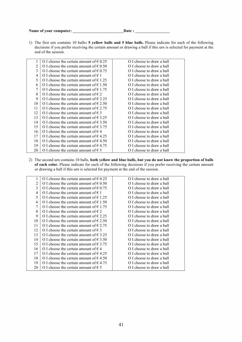
41

Name of your computer: _________________________Date : _________________

1) The first urn contains 10 balls: 5 yellow balls and 5 blue balls. Please indicate for each of the following

decisions if you prefer receiving the certain amount or drawing a ball if this urn is selected for payment at the end of the session. 1 2 3 4 5 6 7 8 9

10 11 12 13 14 15 16 17 18 19 20

O I choose the certain amount of € 0.25 O I choose the certain amount of € 0.50 O I choose the certain amount of € 0.75 O I choose the certain amount of € 1 O I choose the certain amount of € 1.25 O I choose the certain amount of € 1.50 O I choose the certain amount of € 1.75 O I choose the certain amount of € 2 O I choose the certain amount of € 2.25 O I choose the certain amount of € 2.50 O I choose the certain amount of € 2.75 O I choose the certain amount of € 3 O I choose the certain amount of € 3.25 O I choose the certain amount of € 3.50 O I choose the certain amount of € 3.75 O I choose the certain amount of € 4 O I choose the certain amount of € 4.25 O I choose the certain amount of € 4.50 O I choose the certain amount of € 4.75 O I choose the certain amount of € 5

O I choose to draw a ball O I choose to draw a ball O I choose to draw a ball O I choose to draw a ball O I choose to draw a ball O I choose to draw a ball O I choose to draw a ball O I choose to draw a ball O I choose to draw a ball O I choose to draw a ball O I choose to draw a ball O I choose to draw a ball O I choose to draw a ball O I choose to draw a ball O I choose to draw a ball O I choose to draw a ball O I choose to draw a ball O I choose to draw a ball O I choose to draw a ball O I choose to draw a ball

2) The second urn contains 10 balls, both yellow and blue balls, but you do not know the proportion of balls

of each color. Please indicate for each of the following decisions if you prefer receiving the certain amount or drawing a ball if this urn is selected for payment at the end of the session.

1 2 3 4 5 6 7 8 9

10 11 12 13 14 15 16 17 18 19 20

O I choose the certain amount of € 0.25 O I choose the certain amount of € 0.50 O I choose the certain amount of € 0.75 O I choose the certain amount of € 1 O I choose the certain amount of € 1.25 O I choose the certain amount of € 1.50 O I choose the certain amount of € 1.75 O I choose the certain amount of € 2 O I choose the certain amount of € 2.25 O I choose the certain amount of € 2.50 O I choose the certain amount of € 2.75 O I choose the certain amount of € 3 O I choose the certain amount of € 3.25 O I choose the certain amount of € 3.50 O I choose the certain amount of € 3.75 O I choose the certain amount of € 4 O I choose the certain amount of € 4.25 O I choose the certain amount of € 4.50 O I choose the certain amount of € 4.75 O I choose the certain amount of € 5

O I choose to draw a ball O I choose to draw a ball O I choose to draw a ball O I choose to draw a ball O I choose to draw a ball O I choose to draw a ball O I choose to draw a ball O I choose to draw a ball O I choose to draw a ball O I choose to draw a ball O I choose to draw a ball O I choose to draw a ball O I choose to draw a ball O I choose to draw a ball O I choose to draw a ball O I choose to draw a ball O I choose to draw a ball O I choose to draw a ball O I choose to draw a ball O I choose to draw a ball

42

Part 2 [The following instructions were distributed after the participant had completed the first part]

Please do not touch your computer before having read these instructions carefully.

During this part, earnings are calculated in points, with 5 points = 1 Euro.

Description of each period In each period, we propose that you perform a counting task. A paragraph of several lines will be displayed on your screen. This paragraph, randomly generated, consists of French words but is meaningless. The task consists of counting the occurrence of a particular letter in this paragraph. You will be able to count the occurrence of four letters successively during the period.

In each period, you have 2 minutes to perform the task. A counter indicates continuously the remaining time. The paragraph changes in each new period and the letters can also differ.

Determination of the results Your earnings for this part depend on the number of letters that you have counted correctly. An answer is considered as correct if it corresponds to the actual occurrence of this letter, plus or minus one. If the computer indicates that your answer is not correct, you cannot change it and you proceed to the next letter.

However, all periods are not paid. You do not know how many periods in total are paid and you do not know in advance which periods are actually paid. You are informed only a posteriori at the end of a period whether this period gave rise to payment or not. The fact that a period gives rise to payment or not is independent of your outcome. If the period gives rise to payment, each correct answer increases your earnings by 1 point [3 points in the two intermittent reinforcement treatments].

Moreover, starting a new period costs you 1 point. This means that as soon as you start a new period, one point is deducted from your earnings, whether this period gives rise to payment or not. In the first period, the cost of starting this period is deducted from your show-up fee.

Training Before starting the first period, you can practice during two periods to familiarize yourself with the task. These practice periods are not taken into account in the calculation of your earnings. At the end of the practice periods, the first period will start automatically. End of part 2 You are required to complete the first 15 periods. Thereafter, it is you who decide when to stop this part. In other words, there is no automatic start of a new period and the next part will start if you decide to stop the current part. At each new period, you must click either on “start a new period” or on “stop definitively”. If you choose to start a new period, 1 point is deducted from your earnings and you can perform the task. When you decide to stop, you must confirm your decision. If you confirm your decision, you cannot restart the current part and you proceed to the next part.

Part 3 and end of the session

When you decide to stop part 2, the instructions for part 3 will be displayed on your screen. This part consists of several questions to which it is important to answer sincerely. Your answers are anonymous and confidential.

At the end of the session, you will be informed when you can leave the room to get paid. THANK YOU FOR REMAINING SILENT IN LEAVING THE ROOM AND NOT COMMUNICATING WITH OTHERS. Please give back the instructions to the experimenter before leaving the room.

-----

If you have any questions regarding these instructions, please raise your hand and we will answer your questions in private.

When ready, you can start the first practice period by clicking the button “Continue” on your screen.

Thank you for not communicating any information about this experiment.

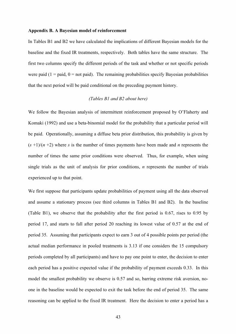
43

Appendix B. A Bayesian model of reinforcement

In Tables B1 and B2 we have calculated the implications of different Bayesian models for the

baseline and the fixed IR treatments, respectively. Both tables have the same structure. The

first two columns specify the different periods of the task and whether or not specific periods

were paid (1 = paid, 0 = not paid). The remaining probabilities specify Bayesian probabilities

that the next period will be paid conditional on the preceding payment history.

(Tables B1 and B2 about here)

We follow the Bayesian analysis of intermittent reinforcement proposed by O’Flaherty and

Komaki (1992) and use a beta-binomial model for the probability that a particular period will

be paid. Operationally, assuming a diffuse beta prior distribution, this probability is given by

(s +1)/(n +2) where s is the number of times payments have been made and n represents the

number of times the same prior conditions were observed. Thus, for example, when using

single trials as the unit of analysis for prior conditions, n represents the number of trials

experienced up to that point.

We first suppose that participants update probabilities of payment using all the data observed

and assume a stationary process (see third columns in Tables B1 and B2). In the baseline

(Table B1), we observe that the probability after the first period is 0.67, rises to 0.95 by

period 17, and starts to fall after period 20 reaching its lowest value of 0.57 at the end of

period 35. Assuming that participants expect to earn 3 out of 4 possible points per period (the

actual median performance in pooled treatments is 3.13 if one considers the 15 compulsory

periods completed by all participants) and have to pay one point to enter, the decision to enter

each period has a positive expected value if the probability of payment exceeds 0.33. In this

model the smallest probability we observe is 0.57 and so, barring extreme risk aversion, no-

one in the baseline would be expected to exit the task before the end of period 35. The same

reasoning can be applied to the fixed IR treatment. Here the decision to enter a period has a

44

positive expected value if the probability of payment exceeds 0.11. Once again, this threshold

is always exceeded such that participants would be expected to enter all periods.

However, participants may also do Bayesian updating with short memories, i.e., not taking all

data into account. If so, in the baseline exiting behavior can be expected after completing

period 21 (last observation, see column 4 in Table B1), period 23 (last 3 observations, see

column 5), period 25 (last 6 observations, see column 6), and 27 (last 10 observations, see

column 7). In the fixed IR treatment, the limited memory models do not all quite provide the

same qualitative picture (see columns 4 to 7 in Table B2). With the shorter memories (last

and last 3 observations), participants are not expected to exit but this tendency reverses itself

as the size of memory increases (last 6 and 10 observations). For the model based on the last

10 observations, participants are expected to exit after period 30.

Finally, we consider a third approach to modeling for the fixed IR treatment (see the last

column of Table B2). Here, we assume memory for all past data but that participants encode

expectations based on pairs of sequences of different types of observations made. In

particular, through period 20 participants should learn that the next period is only paid if the

two preceding periods were not paid (and not paid if one of the two preceding periods is

paid). The unit of analysis of the Bayesian updating model is therefore two successive

observations. The beliefs (probabilities) captured by this model reflect the fact that every

third period is paid starting in period 5 through period 20 (that is, before the probability is

changed to zero). From period 22 on, however, the model breaks down because although

every observation now follows two periods that were not paid, the previously reinforced rule

works no longer (i.e., payment after two successive non-payments). Moreover, whereas the

probability does decrease after period 22, it is still 0.32 at the end of period 35 (i.e., much

larger than 0.11). In short, unless participants exit after period 20 or 21, the model predicts

continuing with the task through period 35.

45

It is important to note that we have not modeled the random IR treatment. This is because the

sequence of actual paid periods varied at random from participant to participant. However,

since the underlying probability is the same as in the fixed IR treatment, one would expect a

similar pattern of probabilities to the fixed IR case, albeit with individual variation.

46

Table B1: Hypothetical probabilities for continuous treatment

Probabilities of payment based on: Continuous Treatment All previous Last Last 3 Last 6 Last 10 Periodd

Paying data observation observations observations observations 1 1 0.67 0.67 x x x 2 1 0.75 0.67 x x x 3 1 0.80 0.67 0.80 x x 4 1 0.83 0.67 0.80 x x 5 1 0.86 0.67 0.80 x x 6 1 0.88 0.67 0.80 0.88 x 7 1 0.89 0.67 0.80 0.88 x 8 1 0.90 0.67 0.80 0.88 x 9 1 0.91 0.67 0.80 0.88 x

10 1 0.92 0.67 0.80 0.88 0.92 11 1 0.92 0.67 0.80 0.88 0.92 12 1 0.93 0.67 0.80 0.88 0.92 13 1 0.93 0.67 0.80 0.88 0.92 14 1 0.94 0.67 0.80 0.88 0.92 15 1 0.94 0.67 0.80 0.88 0.92 16 1 0.94 0.67 0.80 0.88 0.92 17 1 0.95 0.67 0.80 0.88 0.92 18 1 0.95 0.67 0.80 0.88 0.92 19 1 0.95 0.67 0.80 0.88 0.92 20 1 0.95 0.67 0.80 0.88 0.92 21 0 0.91 0.33 0.60 0.75 0.83 22 0 0.88 0.33 0.40 0.63 0.75 23 0 0.84 0.33 0.20 0.50 0.67 24 0 0.81 0.33 0.20 0.38 0.58 25 0 0.78 0.33 0.20 0.25 0.50 26 0 0.75 0.33 0.20 0.13 0.42 27 0 0.72 0.33 0.20 0.13 0.33 28 0 0.70 0.33 0.20 0.13 0.25 29 0 0.68 0.33 0.20 0.13 0.17 30 0 0.66 0.33 0.20 0.13 0.08 31 0 0.64 0.33 0.20 0.13 0.08 32 0 0.62 0.33 0.20 0.13 0.08 33 0 0.60 0.33 0.20 0.13 0.08 34 0 0.58 0.33 0.20 0.13 0.08 35 0 0.57 0.33 0.20 0.13 0.08

1 = paid 0 = not paid Probabilities equal to or less than 0.33 are underlined .

47