THE JOURNAL OF CHEMICAL PHYSICS 138, 194502 (2013)

Intermolecular interactions and the thermodynamic propertiesof supercritical fluids

Tesfaye M. Yigzawe and Richard J. Sadusa)

Centre for Molecular Simulation, Swinburne University of Technology, PO Box 218, Hawthorn,Victoria 3122, Australia

(Received 24 February 2013; accepted 19 April 2013; published online 16 May 2013)

The role of different contributions to intermolecular interactions on the thermodynamic propertiesof supercritical fluids is investigated. Molecular dynamics simulation results are reported for theenergy, pressure, thermal pressure coefficient, thermal expansion coefficient, isothermal and adia-batic compressibilities, isobaric and isochoric heat capacities, Joule-Thomson coefficient, and speedof sound of fluids interacting via both the Lennard-Jones and Weeks-Chandler-Andersen potentials.These properties were obtained for a wide range of temperatures, pressures, and densities. For eachthermodynamic property, an excess value is determined to distinguish between attraction and repul-sion. It is found that the contributions of intermolecular interactions have varying effects dependingon the thermodynamic property. The maxima exhibited by the isochoric and isobaric heat capacities,isothermal compressibilities, and thermal expansion coefficient are attributed to interactions in theLennard-Jones well. Repulsion is required to obtain physically realistic speeds of sound and both re-pulsion and attraction are necessary to observe a Joule-Thomson inversion curve. Significantly, bothmaxima and minima are observed for the isobaric and isochoric heat capacities of the supercriticalLennard-Jones fluid. It is postulated that the loci of these maxima and minima converge to a com-mon point via the same power law relationship as the phase coexistence curve with an exponent ofβ = 0.32. This provides an explanation for the terminal isobaric heat capacity maximum in super-critical fluids. © 2013 AIP Publishing LLC. [http://dx.doi.org/10.1063/1.4803855]

I. INTRODUCTION

Thermodynamic properties have an important role inmany biological, chemical, physical, and technical processes.Considerable emphasis has been placed on modelling andpredicting thermodynamic properties using empirical corre-lations, statistical theories, and equations of state.1, 2 Molecu-lar simulation3 is a useful alternative to conventional theoriesbecause, when used properly, it provides unambiguous infor-mation regarding the merit of the underlying model. Increas-ingly, molecular simulation is being used to provide worth-while predictions to both guide and supplement experimentalwork.

In general, the use of molecular simulation requires thea priori postulation of an intermolecular potential to evalu-ate inter-particle forces or energies. The Lennard-Jones (LJ)potential is arguably the most commonly used intermolecularpotential because it incorporates the salient features of inter-particle interactions. For the LJ potential, the intermolecularenergy (u) between particles i and j separated by a distance rij

is obtained from

u(rij ) = 4ε

((σ

rij

)12

−(

σ

rij

)6)

, (1)

where ε and σ are the characteristic energy and distance pa-rameters, respectively. Equation (1) represents the most com-monly used “12-6” variant of the LJ potential whereas other

a)Email: rsadus@swin.edu.au

choices of exponents are possible resulting in different ob-served behavior.4 The LJ potential incorporates both attractiveand repulsive interactions. Despite its relative simplicity, theLJ potential can reproduce the full range of fluid properties,including both solid-liquid4 and vapor-liquid coexistence.5

Although the LJ potential applies primarily to atomic systemsor small molecules, it is also commonly used in the develop-ment of force fields3 for macromolecules.

It has long been recognised1 that the properties of fluidsare often dominated by repulsive interactions and various sep-arations of the contributions of inter-particle interactions havebeen suggested. McQuarrie and Katz6 proposed a separationof the LJ potential based on the r−12 and r−6 terms. Barker andHenderson7 separated the LJ potential based on regions thatyield positive (rij < σ ) and negative (rij > σ ) values. Weekset al.8 identified purely repulsive and attractive contributionsby splitting the LJ potential at a separation of rij = 21/6σ . Therepulsive part of this separation is now commonly referred toas the Weeks-Chandler-Anderson (WCA) potential. It is theLJ potential truncated at the minimum potential energy at adistance rij = 21/6σ on the length scale and shifted upwardsby the amount ε on the energy scale such that both the energyand force are zero at or beyond the cut-off distance

u(rij ) =

⎧⎪⎨⎪⎩

4ε

((σ

rij

)12

−(

σ

rij

)6)

+ ε, rij ≤ 21/6σ

0 rij > 21/6σ

.

(2)

0021-9606/2013/138(19)/194502/11/$30.00 © 2013 AIP Publishing LLC138, 194502-1

Reuse of AIP Publishing content is subject to the terms: https://publishing.aip.org/authors/rights-and-permissions. Downloaded to IP: 136.186.72.15 On: Mon, 03 Oct 2016

05:07:17

194502-2 T. M. Yigzawe and R. J. Sadus J. Chem. Phys. 138, 194502 (2013)

Equation (2) is a purely repulsive potential as such itcan be only used for a limited range of properties. Forexample, it predicts solid-liquid equilibria but not vapor-liquid equilibria.

The LJ and WCA potentials have been widely investi-gated either as stand alone potentials or they have been in-corporated as part of force fields for molecular systems.9, 10 Inparticular, the phase behavior of the LJ and WCA potentials isvery well documented in the literature.3, 4, 11 However, knowl-edge of the thermodynamic properties of the LJ and WCApotentials remains incomplete with available molecular simu-lation data largely confined12 to quantities such as pressure(p), potential energy (U), isochoric (CV) and isobaric (Cp)heat capacities. In contrast, other thermodynamic propertiessuch as the thermal pressure coefficient (γ v), thermal expan-sion coefficient (αp), isothermal (βT) and adiabatic (βS) com-pressibilities, Joule-Thomson coefficient (μjT), and the speedof sound (w0) are much less commonly reported.13–16 Further-more, simulations of thermodynamic properties in general areoften confined to state points at ambient temperatures.

The relative lack of data can be partly attributed to thefact that only a few thermodynamic properties can be ob-served directly from conventional molecular simulations. TheU, p, and temperature (T) are the only directly observablequantities available from microcanonical (NVE) ensemblesimulations, which maintain a constant number of particles(N), volume (V), and total energy (E). This means that the cal-culation of other thermodynamic quantities requires the useof fluctuation formulas or equations of state.17, 18 Lustig19–22

showed that, in principle, it is possible to calculate all thermo-dynamic state variables from key derivatives obtained directlyfrom either molecular dynamics (MD) or Monte Carlo (MC)simulations. The method is based on the exact expressions forthe thermodynamic state variables in the NV E �P �G ensemble,which maintains both constant linear momentum ( �P ) and anadditional quantity ( �G) that is related to the initial position ofthe center of mass.

The advantage of the NV E �P �G method is that it allowsus to directly obtain all the thermodynamic quantities of afluid from a single MD simulation. We will utilize this fea-

ture to comprehensively determine the full range of thermo-dynamic properties over a wide range of supercritical statepoints. By directly comparing the LJ and WCA results, ouraim is to determine the role of different aspects of molecu-lar interactions. The focus of this work is the near supercrit-ical region in which fluids exhibit interesting behavior suchas percolation transitions in water.23 In particular, we investi-gate the occurrence of maxima and minima in thermodynamicproperties in the supercritical phase.

II. MD SIMULATIONS

A. Overview of the NVE �P �G method

The method has been discussed in detail in Refs. 19, 24,and 25 and only a brief outline of the salient features is givenhere. The fundamental equation of state for the system is de-fined by the entropy (S) postulate,24 i.e.,

S(N,V,E, �P , �G) = k ln �(N,V,E, �P , �G), (3)

where �(N,V,E, �P , �G) is the phase-space volume and k isthe Boltzmann constant. The basic phase-space functions arethen introduced as an abbreviation representing the deriva-tives of the phase-space volume with respect to the indepen-dent thermodynamic state variables

�mn = 1

ω

∂m+n�

∂Em∂V n, (4)

where ω is the phase-space density. The exact derivation ofthe phase-space function is quite involved and the full expres-sion is given in Ref. 24. A feature of the determination of the� terms is the evaluation of volume derivatives of the poten-tial energy

∂nU

∂V n= 1

3nV n

N−1∑i=1

N∑j=i+1

n∑k=1

an krki j

∂ku

∂rki j

, (5)

where the coefficients an k are constructed using a recursionrelation. All thermodynamic state variables are then express-ible in terms of the phase-space function. The resulting ther-modynamic state variables used in this work are summa-rized in Table I. In effect, the NV E �P �G ensemble simulations

TABLE I. Thermodynamic properties expressed in terms of phase-space functions.

Temperature T = (∂E∂S

)V

= � 00k

Pressure p = T(

∂S∂V

)E

= � 01

Isochoric heat capacity CV =[(

∂2S

∂E2

)V

]− 1 = k (1 − � 00 � 20)−1

Thermal pressure coefficient γV =(

∂p∂T

)V

= k� 11−� 01 � 20

1−� 00 � 20

Isothermal compressibility β−1T = −V

(∂p∂V

)T

= V

[�01(2�11−�01�20)−�00�2

111−�00�20

− �02

]

Adiabatic compressibility β−1S = −V

(∂p∂V

)S

= V [�01 (2�11 − �01�20) − �02]

Speed of sound w20 = − V 2

M

(∂p∂V

)S

= V 2

M[�01 (2�11 − �01�20) − �02]

Thermal expansion coefficient αP = βT γV

Isobaric heat capacity CP = CVβTβS

Joule-Thomson coefficient μJ T = VT γV βT −1

CP

Reuse of AIP Publishing content is subject to the terms: https://publishing.aip.org/authors/rights-and-permissions. Downloaded to IP: 136.186.72.15 On: Mon, 03 Oct 2016

05:07:17

194502-3 T. M. Yigzawe and R. J. Sadus J. Chem. Phys. 138, 194502 (2013)

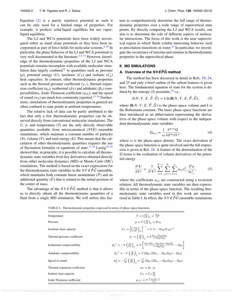
FIG. 1. U as a function of (a) density at different temperatures correspond-ing to ϕ = 1.17 (black �), 1.4 (blue �), 1.6 (pink �), 1.8 (green �), and 2.0(dark blue �); and (b) temperature at different densities corresponding to ρ

= 0.1 (black �), 0.2 (red ●), 0.25 (blue �), 0.3 (pink �), 0.35 (green �), and0.4 (dark blue �). The solid lines are for guidance only.

simply involve implementing a conventional NV E �P simula-tion while keeping track of the volume derivatives of the in-termolecular potential required for the evaluation of the ther-modynamic quantities.

B. Simulation details

The NV E �P �G MD simulations were performed fora homogenous fluid of 2000 particles interacting viathe LJ and WCA potentials. The normal conventionswere used for the reduced density (ρ∗ = ρσ 3), tem-perature (T ∗ = kT/ε), potential energy (U∗ = U/Nε),pressure (p∗ = pσ 3/ε), heat capacities (C∗

p,V = Cp,V /k),compressibilities (β∗

T ,S = βT,S ε/σ 3), thermal pressure co-efficient (γ ∗

V = γV σ 3/k), thermal expansion coefficient(α∗

P = αP ε/k), speed of sound (w∗0 = w0

√m/ε), where m is

the mass of the particles, and the Joule-Thomson coefficient(μ∗

J T = μJ T k/σ 3). All quantities quoted in this work are interms of these reduced quantities and the asterisk superscriptwill be omitted in the rest of the paper.

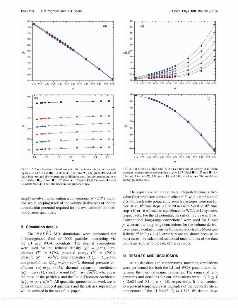
FIG. 2. (a) p for a LJ fluid and (b) p as a function of density at differentconstant temperatures corresponding to ϕ = 1.17 (black �), 1.25 (red ●), 1.4(blue �), 1.6 (pink �), 1.8 (green �), and 2.0 (dark blue �). The solid linesare for guidance only.

The equations of motion were integrated using a five-value Gear predictor-corrector scheme3, 24 with a time step of2 fs. For each state point, simulation trajectories were run for6 or 10 × 106 time steps (12 or 20 ns) with 5 or 8 × 106 timesteps (10 or 16 ns) used to equilibrate the WCA or LJ systems,respectively. For the LJ potential, the cut-off radius was 6.5 σ .Conventional long-range corrections3 were used for U andp, whereas the long-range corrections for the volume deriva-tives were calculated from the formulas reported by Meier andKabelac.24 In Figs. 1–12, error bars are not shown because, inmost cases, the calculated statistical uncertainties of the datapoints are similar to the size of the symbols.

III. RESULTS AND DISCUSSION

At all densities and temperatures, matching simulationswere performed for both the LJ and WCA potentials to de-termine the thermodynamic properties. The ranges of tem-peratures and densities for our simulations were 1.312 ≤ T≤ 2.624 and 0.1 ≤ ρ ≤ 1.0, respectively. It is convenientto represent temperatures as multiples of the reduced criticaltemperature of the LJ fluid,27 Tc = 1.312. We denote these

Reuse of AIP Publishing content is subject to the terms: https://publishing.aip.org/authors/rights-and-permissions. Downloaded to IP: 136.186.72.15 On: Mon, 03 Oct 2016

05:07:17

194502-4 T. M. Yigzawe and R. J. Sadus J. Chem. Phys. 138, 194502 (2013)

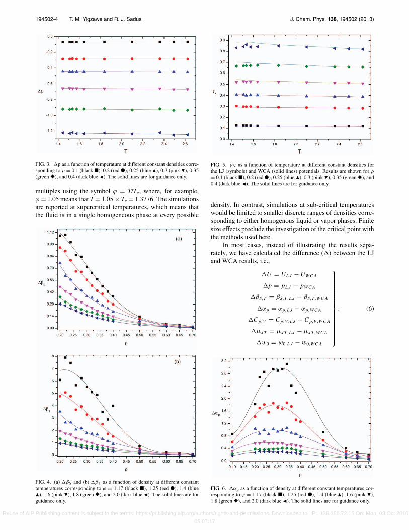
FIG. 3. p as a function of temperature at different constant densities corre-sponding to ρ = 0.1 (black �), 0.2 (red ●), 0.25 (blue �), 0.3 (pink �), 0.35(green �), and 0.4 (dark blue �). The solid lines are for guidance only.

multiples using the symbol ϕ = T/Tc, where, for example,ϕ = 1.05 means that T = 1.05 × Tc = 1.3776. The simulationsare reported at supercritical temperatures, which means thatthe fluid is in a single homogeneous phase at every possible

FIG. 4. (a) βS and (b) βT as a function of density at different constanttemperatures corresponding to ϕ = 1.17 (black �), 1.25 (red ●), 1.4 (blue�), 1.6 (pink �), 1.8 (green �), and 2.0 (dark blue �). The solid lines are forguidance only.

FIG. 5. γ V as a function of temperature at different constant densities forthe LJ (symbols) and WCA (solid lines) potentials. Results are shown for ρ

= 0.1 (black �), 0.2 (red ●), 0.25 (blue �), 0.3 (pink �), 0.35 (green �), and0.4 (dark blue �). The solid lines are for guidance only.

density. In contrast, simulations at sub-critical temperatureswould be limited to smaller discrete ranges of densities corre-sponding to either homogenous liquid or vapor phases. Finitesize effects preclude the investigation of the critical point withthe methods used here.

In most cases, instead of illustrating the results sepa-rately, we have calculated the difference () between the LJand WCA results, i.e.,

U = ULJ − UWCA

p = pLJ − pWCA

βS,T = βS,T ,LJ − βS,T ,WCA

αp = αp,LJ − αp,WCA

Cp,V = Cp,V,LJ − Cp,V,WCA

μJT = μJT,LJ − μJT,WCA

w0 = w0,LJ − w0,WCA

⎫⎪⎪⎪⎪⎪⎪⎪⎪⎪⎪⎪⎪⎪⎬⎪⎪⎪⎪⎪⎪⎪⎪⎪⎪⎪⎪⎪⎭

. (6)

FIG. 6. αp as a function of density at different constant temperatures cor-responding to ϕ = 1.17 (black �), 1.25 (red ●), 1.4 (blue �), 1.6 (pink �),1.8 (green �), and 2.0 (dark blue �). The solid lines are for guidance only.

Reuse of AIP Publishing content is subject to the terms: https://publishing.aip.org/authors/rights-and-permissions. Downloaded to IP: 136.186.72.15 On: Mon, 03 Oct 2016

05:07:17

194502-5 T. M. Yigzawe and R. J. Sadus J. Chem. Phys. 138, 194502 (2013)

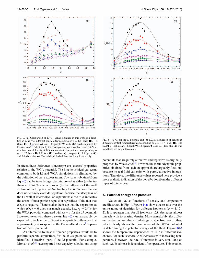
FIG. 7. (a) Comparison of LJ CV values obtained in this work as a func-tion of density at different constant temperatures of T = 1.3 (black �), 1.4(blue ●), 1.6 (green �), and 1.8 (purple �) with MC results reported byFreasier et al.33 (identified by the corresponding open symbols); and (b) CVas a function of density at different constant temperatures corresponding toϕ = 1.17 (black �), 1.25 (red ●), 1.4 (blue �), 1.6 (pink �), 1.8 (green �),and 2.0 (dark blue �). The solid and dashed lines are for guidance only.

In effect, these difference values represent “excess” propertiesrelative to the WCA potential. The kinetic or ideal gas term,common to both LJ and WCA simulations, is eliminated bythe definition of these excess terms. The values obtained fromEq. (6) can be interchangeably interpreted as either (a) the in-fluence of WCA interactions or (b) the influence of the wellsection of the LJ potential. Subtracting the WCA contributiondoes not entirely exclude repulsion because the steepness ofthe LJ well at intermolecular separations close to σ indicatesthe onset of inter-particle repulsion regardless of the fact thatu(rij) is negative. There is also the issue that the separation atwhich u(rij) = 0 does not match exactly, i.e., rij = 21/6σ forthe WCA potential compared with rij = σ for the LJ potential.However, even with these caveats, Eq. (6) can reasonably beexpected to isolate the different inter-particle influences thatapproximately correspond to the Barker-Henderson7 separa-tion of the LJ potential.

An alternative to these difference properties, would be toperform separate simulations for the WCA potential and anidentified “attractive” part of the LJ potential. For example,Morsali et al.26 have reported heat capacity calculations using

FIG. 8. (a) Cp for the LJ potential and (b) Cp as a function of density atdifferent constant temperatures corresponding to ϕ = 1.17 (black �), 1.25(red ●), 1.4 (blue �), 1.6 (pink �), 1.8 (green �), and 2.0 (dark blue �). Thesolid lines are for guidance only.

potentials that are purely attractive and repulsive as originallyproposed by Weeks et al.8 However, the thermodynamic prop-erties obtained from such an approach are arguably fictitiousbecause no real fluid can exist with purely attractive interac-tions. Therefore, the difference values reported here provide amore realistic indication of the contribution from the differenttypes of interaction.

A. Potential energy and pressure

Values of U as functions of density and temperatureare illustrated in Fig. 1. Figure 1(a) shows the results over theentire range of densities for different isotherms (ϕ = 1.17–2). It is apparent that, for all isotherms, U decreases almostlinearly with increasing density. More remarkably, the differ-ent isotherms are almost indistinguishable from each other,which clearly shows the dominance of the WCA potentialin determining the potential energy of the fluid. Figure 1(b)shows the temperature dependence of U at different iso-chores. For each isochore, U increases with increasing tem-perature. However, the rate of increase is very small and assuch U is almost independent of temperature. This enables

Reuse of AIP Publishing content is subject to the terms: https://publishing.aip.org/authors/rights-and-permissions. Downloaded to IP: 136.186.72.15 On: Mon, 03 Oct 2016

05:07:17

194502-6 T. M. Yigzawe and R. J. Sadus J. Chem. Phys. 138, 194502 (2013)

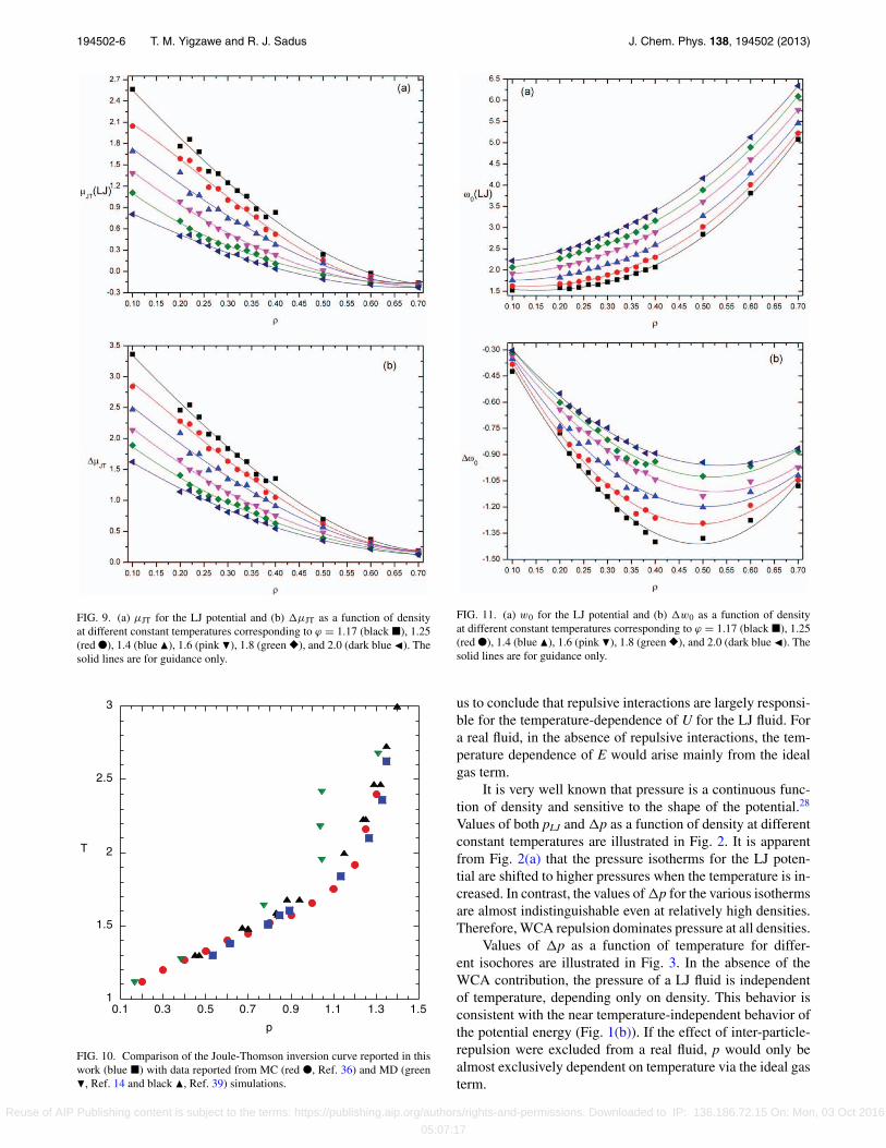
FIG. 9. (a) μJT for the LJ potential and (b) μJT as a function of densityat different constant temperatures corresponding to ϕ = 1.17 (black �), 1.25(red ●), 1.4 (blue �), 1.6 (pink �), 1.8 (green �), and 2.0 (dark blue �). Thesolid lines are for guidance only.

1

1.5

2

2.5

3

0.1 0.3 0.5 0.7 0.9 1.1 1.3 1.5

T

p

FIG. 10. Comparison of the Joule-Thomson inversion curve reported in thiswork (blue �) with data reported from MC (red ●, Ref. 36) and MD (green�, Ref. 14 and black �, Ref. 39) simulations.

FIG. 11. (a) w0 for the LJ potential and (b) w0 as a function of densityat different constant temperatures corresponding to ϕ = 1.17 (black �), 1.25(red ●), 1.4 (blue �), 1.6 (pink �), 1.8 (green �), and 2.0 (dark blue �). Thesolid lines are for guidance only.

us to conclude that repulsive interactions are largely responsi-ble for the temperature-dependence of U for the LJ fluid. Fora real fluid, in the absence of repulsive interactions, the tem-perature dependence of E would arise mainly from the idealgas term.

It is very well known that pressure is a continuous func-tion of density and sensitive to the shape of the potential.28

Values of both pLJ and p as a function of density at differentconstant temperatures are illustrated in Fig. 2. It is apparentfrom Fig. 2(a) that the pressure isotherms for the LJ poten-tial are shifted to higher pressures when the temperature is in-creased. In contrast, the values of p for the various isothermsare almost indistinguishable even at relatively high densities.Therefore, WCA repulsion dominates pressure at all densities.

Values of p as a function of temperature for differ-ent isochores are illustrated in Fig. 3. In the absence of theWCA contribution, the pressure of a LJ fluid is independentof temperature, depending only on density. This behavior isconsistent with the near temperature-independent behavior ofthe potential energy (Fig. 1(b)). If the effect of inter-particle-repulsion were excluded from a real fluid, p would only bealmost exclusively dependent on temperature via the ideal gasterm.

Reuse of AIP Publishing content is subject to the terms: https://publishing.aip.org/authors/rights-and-permissions. Downloaded to IP: 136.186.72.15 On: Mon, 03 Oct 2016

05:07:17

194502-7 T. M. Yigzawe and R. J. Sadus J. Chem. Phys. 138, 194502 (2013)

0.8

1.2

1.6

2

2.4

2.8

3.2

0 0.2 0.4 0.6 0.8 1

T

ρ

vapor and liquid

CP

TE(Cv)

TE(Cp)

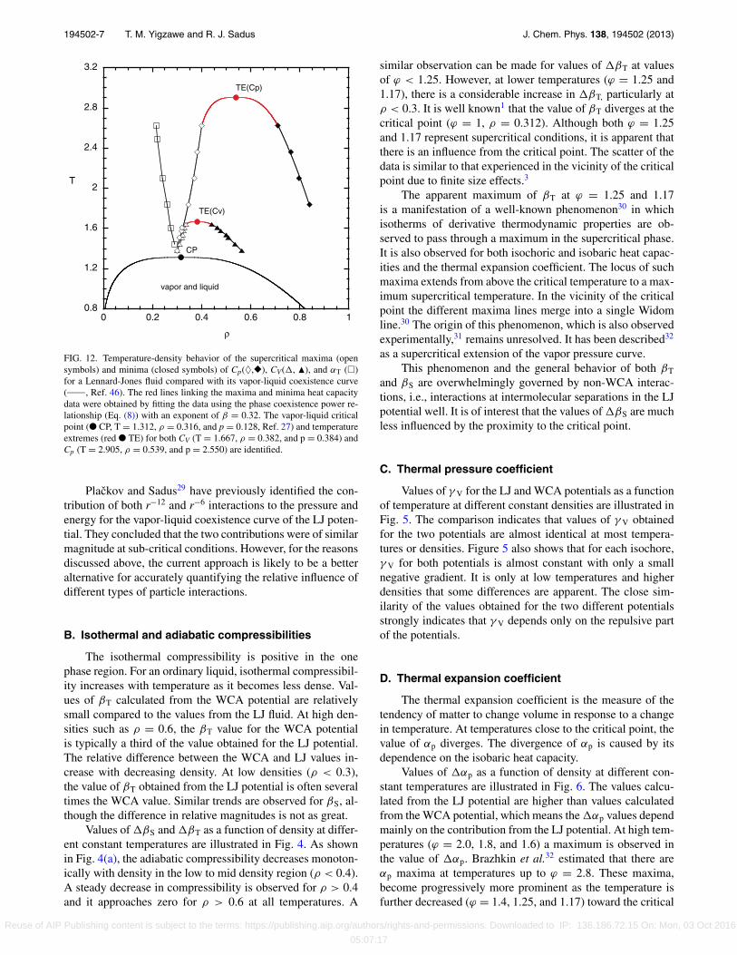
FIG. 12. Temperature-density behavior of the supercritical maxima (opensymbols) and minima (closed symbols) of Cp(♦,�), CV(, �), and αT (�)for a Lennard-Jones fluid compared with its vapor-liquid coexistence curve(_____, Ref. 46). The red lines linking the maxima and minima heat capacitydata were obtained by fitting the data using the phase coexistence power re-lationship (Eq. (8)) with an exponent of β = 0.32. The vapor-liquid criticalpoint (● CP, T = 1.312, ρ = 0.316, and p = 0.128, Ref. 27) and temperatureextremes (red ● TE) for both CV (T = 1.667, ρ = 0.382, and p = 0.384) andCp (T = 2.905, ρ = 0.539, and p = 2.550) are identified.

Plackov and Sadus29 have previously identified the con-tribution of both r−12 and r−6 interactions to the pressure andenergy for the vapor-liquid coexistence curve of the LJ poten-tial. They concluded that the two contributions were of similarmagnitude at sub-critical conditions. However, for the reasonsdiscussed above, the current approach is likely to be a betteralternative for accurately quantifying the relative influence ofdifferent types of particle interactions.

B. Isothermal and adiabatic compressibilities

The isothermal compressibility is positive in the onephase region. For an ordinary liquid, isothermal compressibil-ity increases with temperature as it becomes less dense. Val-ues of βT calculated from the WCA potential are relativelysmall compared to the values from the LJ fluid. At high den-sities such as ρ = 0.6, the βT value for the WCA potentialis typically a third of the value obtained for the LJ potential.The relative difference between the WCA and LJ values in-crease with decreasing density. At low densities (ρ < 0.3),the value of βT obtained from the LJ potential is often severaltimes the WCA value. Similar trends are observed for βS, al-though the difference in relative magnitudes is not as great.

Values of βS and βT as a function of density at differ-ent constant temperatures are illustrated in Fig. 4. As shownin Fig. 4(a), the adiabatic compressibility decreases monoton-ically with density in the low to mid density region (ρ < 0.4).A steady decrease in compressibility is observed for ρ > 0.4and it approaches zero for ρ > 0.6 at all temperatures. A

similar observation can be made for values of βT at valuesof ϕ < 1.25. However, at lower temperatures (ϕ = 1.25 and1.17), there is a considerable increase in βT, particularly atρ < 0.3. It is well known1 that the value of βT diverges at thecritical point (ϕ = 1, ρ = 0.312). Although both ϕ = 1.25and 1.17 represent supercritical conditions, it is apparent thatthere is an influence from the critical point. The scatter of thedata is similar to that experienced in the vicinity of the criticalpoint due to finite size effects.3

The apparent maximum of βT at ϕ = 1.25 and 1.17is a manifestation of a well-known phenomenon30 in whichisotherms of derivative thermodynamic properties are ob-served to pass through a maximum in the supercritical phase.It is also observed for both isochoric and isobaric heat capac-ities and the thermal expansion coefficient. The locus of suchmaxima extends from above the critical temperature to a max-imum supercritical temperature. In the vicinity of the criticalpoint the different maxima lines merge into a single Widomline.30 The origin of this phenomenon, which is also observedexperimentally,31 remains unresolved. It has been described32

as a supercritical extension of the vapor pressure curve.This phenomenon and the general behavior of both βT

and βS are overwhelmingly governed by non-WCA interac-tions, i.e., interactions at intermolecular separations in the LJpotential well. It is of interest that the values of βS are muchless influenced by the proximity to the critical point.

C. Thermal pressure coefficient

Values of γ V for the LJ and WCA potentials as a functionof temperature at different constant densities are illustrated inFig. 5. The comparison indicates that values of γ V obtainedfor the two potentials are almost identical at most tempera-tures or densities. Figure 5 also shows that for each isochore,γ V for both potentials is almost constant with only a smallnegative gradient. It is only at low temperatures and higherdensities that some differences are apparent. The close sim-ilarity of the values obtained for the two different potentialsstrongly indicates that γ V depends only on the repulsive partof the potentials.

D. Thermal expansion coefficient

The thermal expansion coefficient is the measure of thetendency of matter to change volume in response to a changein temperature. At temperatures close to the critical point, thevalue of αp diverges. The divergence of αp is caused by itsdependence on the isobaric heat capacity.

Values of αp as a function of density at different con-stant temperatures are illustrated in Fig. 6. The values calcu-lated from the LJ potential are higher than values calculatedfrom the WCA potential, which means the αp values dependmainly on the contribution from the LJ potential. At high tem-peratures (ϕ = 2.0, 1.8, and 1.6) a maximum is observed inthe value of αp. Brazhkin et al.32 estimated that there areαp maxima at temperatures up to ϕ = 2.8. These maxima,become progressively more prominent as the temperature isfurther decreased (ϕ = 1.4, 1.25, and 1.17) toward the critical

Reuse of AIP Publishing content is subject to the terms: https://publishing.aip.org/authors/rights-and-permissions. Downloaded to IP: 136.186.72.15 On: Mon, 03 Oct 2016

05:07:17

194502-8 T. M. Yigzawe and R. J. Sadus J. Chem. Phys. 138, 194502 (2013)

temperature of the LJ fluid. The growing influence of the crit-ical point is apparent in the scatter of the data, which indicatesthat finite size effects are important in the supercritical phase.This phenomenon can be attributed to interactions at inter-particle separations in the well of the LJ potential because itoccurs both in the presence and absence of WCA interactions.

E. Isochoric and isobaric heat capacities

Values of CV for the LJ fluid at supercritical tempera-tures have been previously reported by Freasier et al.33 fromMonte Carlo simulations using the conventional fluctuationformula.17, 18 Our results for the LJ fluid are compared withthese data in Fig. 7(a). At high temperatures (T = 1.8 and1.6), there is good agreement between the two sets of data.At T = 1.4, the data are in agreement at most densities, ex-cept near the maximum in Cv. However at T = 1.3, we ob-serve a much larger maximum in CV. These differences canbe largely attributed to the fact that Freasier et al.33 truncatedthe LJ potential at a cut-off value of 2.5σ . Our calculations arefor the full LJ potential with a cut-off distance of 6.5σ , whichis considerably larger than 2.5σ . It is very well documented34

that properties of fluids are sensitive to this, particularly inthe vicinity of the critical point. At the lower temperatures, aminimum in CV is also observed at a density of approximatelyρ = 0.6.

A feature of the simulation results that is shared by realfluids is the observation of a maximum in CV at supercriti-cal temperatures. As discussed above, in the vicinity of thecritical point the locus of these maxima form a so-calledWidom line.30 Hess et al.35 have previously reported exten-sive CV data for WCA particles and some LJ data have beenreported recently.16 For any given supercritical isotherm, val-ues of CV obtained from the WCA potential increase mono-tonically with increasing density. Our results for the WCApotential are in good agreement with these data. The absenceof a maximum for the WCA potential indicates that this phe-nomenon can be attributed to interactions occurring at sepa-rations corresponding to the minimum of the LJ potential.

Isothermal values of CV as a function of density areillustrated in Fig. 7(b). The relatively small values of CV

illustrate the dominance of WCA interactions in determin-ing the magnitude of CV. A peak in CV is observed for allisotherms but the phenomenon is much more pronounced attemperatures approaching the critical temperature (ϕ = 1.17and 1.25). At these temperatures, there is a noticeable scatterin the data compared with higher temperatures (ϕ = 1.6, 1.8,and 2.0), which can be attributed to the influence of finite sizeeffects.35–37 Despite the dominance of WCA interactions indetermining the overall magnitude of CV, it is clear from thiscomparison that interactions associated with the well of theLJ potential are the controlling influence responsible for theCV maxima.

Isothermal values of Cp for the LJ potential as a functionof density are illustrated in Fig. 8(a). Most of the trends ob-served in Cp are the same as observed for CV and the sameconclusions can be applied. However, the WCA interactionshave a relatively minor influence on the magnitude of Cp.

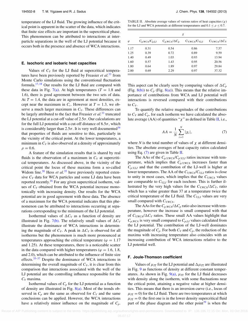
TABLE II. Absolute average values of various ratios of heat capacities (χ )for the LJ and WCA potentials at different temperatures and 0.1 ≤ ρ ≤ 0.7.

χ

ϕ Cp,WCA/Cp,LJ Cp,WCA/Cp CV,WCA/CV,LJ CV,WCA/CV

1.17 0.31 0.54 0.86 7.571.25 0.39 0.72 0.89 9.591.40 0.49 1.03 0.93 13.941.60 0.57 1.43 0.95 20.561.80 0.64 1.89 0.97 29.842.00 0.69 2.29 0.97 37.32

This aspect can be clearly seen by comparing values of Cp

(Fig. 8(b)) to Cp (Fig. 8(a)). This means that the relative im-portance of contributions from WCA and LJ potential wellinteractions is reversed compared with their contributionsto CV.

To quantify the relative magnitudes of the contributionsto CV and Cp, for each isotherm we have calculated the abso-lute average (AA) of quantities “χ” as defined in Table II, i.e.,

AA = 1

N

N∑i=1

|χi |, (7)

where N is the total number of values of χ at different densi-ties. The absolute averages of heat capacity ratios calculatedusing Eq. (7) are given in Table II.

The AAs of the Cp,V,WCA/Cp,V,LJ ratios increase with tem-perature, which implies that Cp,V,WCA increases faster thanCp,V,LJ and that the contribution of the LJ-well is higher atlower temperatures. The AA of the CV,WCA/CV,LJ ratios is closeto unity in most cases, which implies that the CV,WCA valuesare comparable to CV,LJ for each isochore. This is further il-lustrated by the very high values for the CV,WCA/CV, ratiowhich has a value greater than 37 at a temperature twice thecritical temperature of the LJ fluid. The CV,LJ values are verysmall compared with CV,WCA.

The AAs for the Cp,WCA/Cp ratio also increase with tem-perature, however the increase is small compared with thatof CV,WCA/CV ratios. These small AA values highlight thatCp,WCA is very small compared to Cp,LJ values calculated fromthe LJ potential. The contribution of the LJ-well dominatesthe magnitude of Cp. For both CV and Cp, the reduction of themaxima with increasing temperature also coincides with anincreasing contribution of WCA interactions relative to theLJ potential well.

F. Joule-Thomson coefficient

Values of μJT for the LJ potential and μJT are illustratedin Fig. 9 as functions of density at different constant temper-atures. As shown in Fig. 9(a), μJT for the LJ fluid decreaseswith density along the isotherm, with some fluctuations nearthe critical point, attaining a negative value at higher densi-ties. This means that there is an inversion curve (i.e., locus ofμJT = 0) for the LJ fluid. There are two temperatures at whichμJT = 0: the first one is in the lower density supercritical fluidpart of the phase diagram and the other point39 is when the

Reuse of AIP Publishing content is subject to the terms: https://publishing.aip.org/authors/rights-and-permissions. Downloaded to IP: 136.186.72.15 On: Mon, 03 Oct 2016

05:07:17

194502-9 T. M. Yigzawe and R. J. Sadus J. Chem. Phys. 138, 194502 (2013)

fluid approaches the liquid state as p → 0. In the region whereμJT > 0 for the LJ fluid (0.1 ≤ ρ ≤ 0.6), the decrease inpressure has caused a decrease in temperature which occursas a result of lower initial pressure. In the region where μJT

> 0 (ρ ≥ 0.6 for the LJ potential and at all densities for theWCA potential), the decrease in pressure causes an increasein temperature, i.e., there will be heating on expansion. Thevalues of μJT from the WCA are negative at all temperaturesand densities, which is reflected in the larger values of μJT

(Fig. 9(b)) compared with μJT for the LJ potential (Fig. 9(a)).An important consequence of the negative contribution fromWCA interactions is that it makes an inversion curve possiblefor the LJ potential.

It should be noted that obtaining the inversion curve is achallenge for both experimental methods and molecular simu-lation. The most extensive calculations of the inversion curvefor the LJ fluid have been reported37, 38 from MC simula-tions. Escobedo and Chen14 reported good results using a MCmulti-histogram re-weighing technique. In contrast, as shownin Fig. 10, Heyes and Llaguno39 reported considerable diffi-culties in accurately locating the inversion curve from con-ventional MD simulation. Kioupis et al.40, 41 addressed thisproblem via a specialised constant enthalpy MD algorithm.

To obtain the inversion curve, we first calculated thedensity at which μJT is zero for each of the isotherms inFig. 9(a). A change in sign takes place when the density isbetween 0.6 and 1.0. We then found the corresponding valueof the pressure at that density from Fig. 2(a) for each of theisotherms. This was achieved by finding the best fit to eachof the isotherms and then using a fitting equation to calcu-late the pressure at each of the densities where μJT = 0. Thisonly results in a partial inversion curve because, as shown inRefs. 42–44, a very large number of simulation results atϕ ≥ 4.5 would be required to obtain the complete inversioncurve. The coordinates for the LJ inversion curve extrapolatedin this way from our simulations are given in Table III and acomparison with literature values is given in Fig. 10.

The comparison in Fig. 10 indicates that our inversiontemperature is in good agreement with the data of Colinaand Müller37 and Kioupis et al.,41 which are consistent withcalculations obtained from a LJ equation of state.45 We didnot observe the difficulties reported by Heyes and Llaguno,39

which suggests that the NV E �P �G MD ensemble is particu-larly beneficial for this property. As noted above, the inver-sion curve is difficult to calculate accurately. Escobedo andChen14 identified factors such as insufficient cycles to accu-mulate simulation averages, system size, and cut-off values aspossible sources of discrepancies. Our system size of 2000 islarger than the 256 (Ref. 14) or 500 (Refs. 14 and 37) parti-cle simulations reported previously; a large cut-off value wasused; and the averages were accumulated for the equivalent of

TABLE III. Coordinates of the partial Joule-Thomson inversion curve forthe Lennard-Jones fluid.

ϕ 1.0 1.05 1.15 1.2 1.225 1.40 1.60 1.80 2.0p 0.530 0.615 0.794 0.847 0.894 1.134 1.266 1.329 1.348ρ 0.637 0.617 0.595 0.589 0.582 0.553 0.510 0.469 0.424

2 × 106 MC cycles compared with 104 (Ref. 37) and 105

(Ref. 14) cycles used elsewhere.

G. Speed of sound

Values of ω0 calculated for the LJ fluid and ω0 are illus-trated in Fig. 11 as a function of density at different constanttemperatures. As shown in Fig. 11(a), ω0 increases with den-sity along each isotherm without any noticeable fluctuationsnear the critical point. The speed of sound approaches a min-imum value near the critical point. The power law expressionfor ω0 at the critical point predicts the speed of sound to bezero.1

The pressure calculated from the WCA potential is higherthan the value calculated from the LJ potential (Fig. 2(b)).The speed of sound depends on pressure (see Table I), whichmeans that values of ω0 for the WCA potential will behigher than that from the LJ potential. The large contributionof WCA interactions is evident from the values of ω0 inFig. 11(b). In the absence of the WCA contribution, ω0 wouldhave physically unrealistic negative values. This highlightsthe important role of repulsion, particularly at small separa-tions, on the thermodynamic properties of fluids.

H. Maxima and minima of thermodynamic properties

We have observed that αp, CV, and Cp obtained for aLennard-Jones fluid have distinct maxima in the supercriti-cal phase, which is entirely consistent with the behavior ofreal fluids. We have also found that both CV and Cp have min-ima at high densities. To the best of our knowledge Cp minimahave not been reported previously for the Lennard-Jones fluid.The loci of both maxima and minima for the thermodynamicproperties are illustrated in Fig. 12 in conjunction with thevapor-liquid phase diagram for a Lennard-Jones fluid.27, 46 Itshould be noted that there is a degree of scatter in the simu-lation data, particularly in the vicinity of the maxima, whichmeans that the coordinates should be treated as approxima-tions only.

As temperature is increased, Fig. 12 shows that the locusof αp maxima veers progressively to densities that are muchless that the critical density (ρ = 0.316, Ref. 27). In commonwith the maxima of all thermodynamic quantities, it becomesless pronounced with increasing temperature and disappearsat an undetermined temperature beyond T = 2.624. This be-havior is consistent with other work in the literature32 for theLennard-Jones fluid.

The behavior of the maxima and minima of CV and Cp

are particularly noteworthy. At all supercritical temperatures,both a maxima and minima were observed for CV. It is ap-parent from Fig. 12 that the CV maxima initially occurs at adensity close to the critical density but progressively shifts tohigher densities. In contrast, the CV minima commences froma relatively high density and progressively shifts to lower den-sities, that is, the loci of CV maxima and CV minima are appar-ently converging to a common point or a shared temperatureextreme (TE) after which no further maxima or minima areobserved. We find that the maxima and minima loci can be

Reuse of AIP Publishing content is subject to the terms: https://publishing.aip.org/authors/rights-and-permissions. Downloaded to IP: 136.186.72.15 On: Mon, 03 Oct 2016

05:07:17

194502-10 T. M. Yigzawe and R. J. Sadus J. Chem. Phys. 138, 194502 (2013)

fitted to the same power law as vapor-liquid equilibria and thedensities are consistent with the law of rectilinear diameters,47

i.e.,

ρmin − ρmax = A

∣∣∣∣1 − T

TE

∣∣∣∣β

(ρmin + ρmax)

2= ρE + C(TE − T )

⎫⎪⎪⎬⎪⎪⎭ , (8)

where A and C are constants. Using a value of β = 0.32, wefind that TE,CV

= 1.667, ρE,CV= 0.382, and pE,CV

= 0.384,where pE,CV

was obtained from an independent simulation atconditions corresponding to TE,CV

and ρE,CV.

Experimental measurements for the isochoric heat capac-ity at supercritical temperatures have been reported,48 whichexhibit both maxima and minima curves that converge at acommon point. Experimental heat capacity data49 for diethylether provide a recent example of both maxima and minimabehavior. The phenomena observed for the Lennard-Jonesfluid are qualitatively similar except that the minima curvefor diethyl ether first veers to lower densities before connect-ing to the maxima curve at a density slightly above the criticaldensity.

At temperatures immediately above the critical point,only maxima in Cp are observed initially. It is evident fromFig. 12 that the densities of the maxima of Cp and CV largelycoincide. However, at temperatures above TE,CV

= 1.657,minima are also observed for Cp. The Cp minima curve com-mences at much higher densities than the corresponding CV

curve. The position of the Cp minima shifts to lower densi-ties with increasing temperatures whereas the Cp maxima islocated at progressively higher densities, which indicates thatthe convergence of the two curves is likely. It is apparent fromFig. 12 that the Cp phenomena occur over a much larger rangeof both density and temperature than for CV. Equation (8) canalso be used to locate the coordinates of the temperature ex-treme, which is found at TE,Cp

= 2.905, ρE,Cp= 0.539, and

pE,Cp= 2.550.

For a given isotherm, maxima in either CV or Cp corre-spond to

(∂Cp,V

∂V

)T <TE>Tc

= 0(∂2Cp,V

∂V 2

)T <TE>Tc

< 0

⎫⎪⎪⎪⎬⎪⎪⎪⎭

(9)

whereas, the occurrence of minima on the isotherm means

(∂Cp,V

∂V

)T <TE>Tc

= 0(∂2Cp,V

∂V 2

)T <TE>Tc

> 0

⎫⎪⎪⎪⎬⎪⎪⎪⎭

. (10)

The convergence of the maxima and minima curves to a com-mon point suggests that this is a point of inflection character-

ized by (∂Cp,V

∂V

)T =TE

= 0(∂2Cp,V

∂V 2

)T =TE

= 0(∂3Cp,V

∂V 3

)T =TE

�= 0

⎫⎪⎪⎪⎪⎪⎪⎪⎪⎬⎪⎪⎪⎪⎪⎪⎪⎪⎭

. (11)

The critical isotherm of a pure fluid also exhibits an inflectionpoint in its pressure-volume behavior. The behavior of heatcapacity in the supercritical region appears analogous to thebehavior of pressure at sub-critical isotherms. Experimentalvalues of pressure are constant along all sub-critical isothermswithin the two-phase region bounded by the coexisting liquidand vapor densities whereas there is a steep pressure gradienton either side of the coexistence curve. Similarly, there is anoticeable heat capacity gradient at densities outside of the re-gion bounded by the maxima and minima densities. Isothermsabove the critical point display a smooth variation in pressureat all densities and similar behavior is observed for heat ca-pacities for isotherms with T > TE.

Previous calculations in the literature32 for the Lennard-Jones potential indicate that the Cp maxima, which initiallytrends towards increasing densities, diverges back to the crit-ical density at high temperatures. To the best of our knowl-edge, the existence of Cp minima have not been previouslyobserved either in the Lennard-Jones fluid or real fluids. Thisis in contrast with experimental evidence48, 49 for the exis-tence of such behavior in CV. The magnitude of the minimais much less pronounced than the maxima and it diminisheswith increasing temperatures. This means that it could be eas-ily overlooked, particularly if the density increments are notsufficiently small. The maxima also diminish with increas-ing temperature and become more difficult to detect at hightemperatures. Heat capacity measurements in the supercriti-cal phase are focused primarily in the region of the maxima,which is often well outside of the region in which minimaare likely to be located. The preference for performing mea-surements at constant pressure also means that densities cor-responding to the minima may not be encountered routinely.

The existence of a locus of minima provides a mechanismfor the hitherto largely unexplained termination of the locusof maxima. The locus of maxima is sometimes interpreted50

as a demarcation point between “gas-like” and “liquid-like”behavior in the supercritical phase. Assuming that such a de-scription is valid, then the locus of minima could be logicallyinterpreted as a second demarcation line.

IV. CONCLUSIONS

The NV E �P �G MD ensemble can be used to directlyobtain all of the thermodynamic properties of supercriticalfluids. The comparison of results obtained for the LJ andWCA potentials provides insights into the contribution ofintermolecular interaction on thermodynamic properties. Animportant insight arising from this work is that the role ofWCA and LJ potential well interactions are different depend-ing on the thermodynamic property. The complexity of the

Reuse of AIP Publishing content is subject to the terms: https://publishing.aip.org/authors/rights-and-permissions. Downloaded to IP: 136.186.72.15 On: Mon, 03 Oct 2016

05:07:17

194502-11 T. M. Yigzawe and R. J. Sadus J. Chem. Phys. 138, 194502 (2013)

thermodynamic properties in terms of the phase-space func-tions means that only general observations can be safely madelinking thermodynamic properties to specific interactions.

The temperature dependence of U can be largely at-tributed to repulsive WCA interactions and in the absence ofsuch interactions the temperature-dependence of p would bealmost entirely due to the ideal gas term. The contributions ofWCA interactions ensure that the LJ potential has a μJT inver-sion curve, which has been partially determined in this work.They also ensure that physically realistic values are obtainedfor w0.

Repulsive interactions have an important role in βT,whereas their contribution to βS is small. The values of γ V

obtained for either the WCA or LJ potentials are almost iden-tical for a large range of both temperatures and densities. Re-pulsion has only a small influence of values of αp, whichpass through a maximum value at supercritical temperaturesin the proximity of the critical point. This behavior is alsoa characteristic of CV and Cp and in both cases it is appar-ent that it is determined by interactions at separations withinthe LJ potential well. The contribution of repulsive interac-tions dominates the magnitude of CV, whereas the attractivepart of the potential is the largest contributor to Cp. In gen-eral, we observe that much of the divergent behavior of αp,βT, CV, and Cp occurs at nearest neighbor separations closeto values corresponding to the minimum of the LJ poten-tial well and as such the influence of WCA interactions isminimal.

At supercritical temperatures, both maxima and minimavalues of CV and Cp are observed for the Lennard-Jones fluid.Supercritical CV and Cp maxima and CV minima are welldocumented from experimental studies of real fluids. In con-trast, the existence of a locus of Cp minima has not been ob-served previously. The maxima and minima loci for both CV

and Cp appear to converge to a common point. We postulatethat the temperature-density behavior of these curves obey thesame power law as the coexistence curve with an exponent ofβ = 0.32. The convergence of the two branches of the Cp

curves provides an alternative explanation for the terminatingvalue of the Cp maxima in supercritical fluids.

ACKNOWLEDGMENTS

We thank the National Computing Infrastructure (NCI)for an allocation of computing time. One of us (T.M.Y.)thanks Swinburne University of Technology for a postgrad-uate research award.

1C. G. Gray and K. E. Gubbins, Theory of Molecular Fluids Vol. 1: Funda-mentals (Clarendon Press, Oxford, 1984); J.-P. Hansen and I. R. McDonald,Theory of Simple Liquids, 2nd ed. (Academic Press, London, 1986).

2Y. S. Wei and R. J. Sadus, AIChE J. 46, 169 (2000).3R. J. Sadus, Molecular Simulation of Fluids: Theory, Algorithms andObject-Orientation (Elsevier, Amsterdam, 1999).

4A. Ahmed and R. J. Sadus, J. Chem. Phys. 131, 174504 (2009).5A. Z. Panagiotopoulos, Mol. Phys. 61, 813 (1987); R. J. Sadus and J. M.Prausnitz, J. Chem. Phys. 104, 4784 (1996).

6D. A. McQuarrie and J. L. Katz, J. Chem. Phys. 44, 2393 (1966).7J. A. Barker and D. Henderson, J. Chem. Phys. 47, 4714 (1967).8J. D. Weeks, D. Chandler, and H. C. Andersen, J. Chem. Phys. 54, 5237(1971).

9M. Kröger, Phys. Rep. 390, 453 (2004).10J. T. Bosko, B. D. Todd, and R. J. Sadus, J. Chem. Phys. 124, 044910

(2006).11A. Ahmed and R. J. Sadus, Phys. Rev. E 80, 061101 (2009).12F. W. de Wette, L. H. Fowler, and B. R. A. Nijboer, Physica 54, 292 (1971);

A. Toro-Labbé, R. Lustig, and W. A. Steele, Mol. Phys. 67, 1385 (1989): D.Boda, T. Lukács, J. Liszi, and I. Szalai, Fluid Phase Equilib. 119, 1 (1996);J. J. Nicolas, K. E. Gubbins, W. B. Streett, and D. J. Tildesley, Mol. Phys.37, 1429 (1979); F. Cuadros, A. Mulero, and W. Ahumada, Thermochim.Acta 277, 85 (1996); F. Cuadros and W. Ahumada, ibid. 297, 109 (1997);F. Cuadros, A. Mulero, and C. A. Faúndez, Mol. Phys. 98, 899 (2000); V.G. Baidokov, S. P. Protsenko, and Z. R. Kozlova, Chem. Phys. Lett. 447,236 (2007).

13R. Lustig, A. Toro-Labbé, and W. A. Steele, Fluid Phase Equilib. 48, 1(1989).

14F. A. Escobedo and Z. Chen, Mol. Simul. 26, 395 (2001).15G. Galliero and C. Boned, J. Chem. Phys. 129, 074506 (2008).16H.-O. May and P. Mausbach, Phys. Rev. E 85, 031201 (2012).17J. L. Lebowitz, J. K. Percus, and L. Verlet, Phys. Rev. 153, 250 (1967).18P. S. Y. Cheung, Mol. Phys. 33, 519 (1977).19R. Lustig, J. Chem. Phys. 100, 3048 (1994).20R. Lustig, J. Chem. Phys. 100, 3060 (1994).21R. Lustig, J. Chem. Phys. 100, 3068 (1994).22R. Lustig, J. Chem. Phys. 109, 8816 (1998).23L. Pártay and P. Jedlovszky, J. Phys. Chem. 123, 024502 (2005); M.

Bernabei, A. Botti, F. Bruni, M. A. Ricci, and K. Soper, Phys. Rev. E 78,021505 (2008); M. Bernabei and M. A. Ricci, J. Phys.: Condens. Matter20, 494208 (2008).

24K. Meier and S. Kabelac, J. Chem. Phys. 124, 064104 (2006).25P. Mausbach and R. J. Sadus, J. Chem. Phys. 134, 114515 (2011).26A. Morsali, S. A. Beyramabadi, S. H. Vahidi, and M. Ghorbani, Mol. Phys.

110, 483 (2012).27J. J. Potoff and A. Z. Panagiotopoulos, J. Chem. Phys. 109, 10914 (1998).28P. S. Vogt, R. Liapine, B. Kirchner, A. J. Dyson, H. Huber, G. Marcelli, and

R. J. Sadus, Phys. Chem. Chem. Phys. 3, 1297 (2001).29Ð. Plackov and R. J. Sadus, Fluid Phase Equilib. 134, 77 (1997).30L. Xu, P. Kumar, S. V. Buldyrev, S.-H. Chen, P. H. Poole, F. Sciortino, and

H. E. Stanley, Proc. Natl. Acad. Sci. U.S.A. 102, 16558 (2005).31Heat Capacities: Liquids, Solutions and Vapours, edited by E. Wilhelm and

T. Letcher (The Royal Society of Chemistry, Cambridge, 2010).32V. V. Brazhkin, Y. D. Fomin, A. G. Lyapin, V. N. Ryzhov, and E. N. Tsiok,

J. Phys. Chem. B 115, 14112 (2011).33B. C. Freasier, A. Czezowski, and R. J. Bearman, J. Chem. Phys. 101, 7934

(1994).34W. Shi and J. K. Johnson, Fluid Phase Equilib. 187–188, 171 (2001).35S. Hess, M. Kröger, and H. Voigt, Physica A 250, 58 (1998).36B. C. Freasier, C. E. Woodward, and R. J. Bearman, J. Chem. Phys. 105,

3686 (1996).37C. Colina and E. A. Müller, Mol. Simul. 19, 237 (1997).38C. M. Colina and E. A. Müller, Int. J. Thermophys. 20, 229 (1999).39D. M. Heyes and C. T. Llaguno, Chem. Phys. 168, 61 (1992).40L. I. Kioupis and E. J. Maginn, Fluid Phase Equilib. 200, 75 (2002).41L. I. Kioupis, G. Arya, and E. J. Maginn, Fluid Phase Equilib. 200, 93

(2002).42Y. Song and E. A. Mason, J. Chem. Phys. 91, 7840 (1989).43J. Kolafa and I. Nezbeda, Fluid Phase Equilib. 100, 1 (1994).44W. W. Wood and F. R. Parker, J. Chem. Phys. 27, 720 (1957).45J. K. Johnson, J. A. Zollweg, and K. E. Gubbins, Mol. Phys. 78, 591 (1993).46D. Kofke, J. Chem. Phys. 98, 4149 (1993).47R. J. Sadus, Mol. Phys. 87, 979 (1996).48A. I. Abdulagatov, G. V. Stepanov, I. M. Abdulagatov, A. E. Ramaznova,

and G. S. Alidultanova, Chem. Eng. Commun. 190, 1499 (2003).49N. G. Polikhronidi, I. M. Abdulagotov, R. G. Butyrova, G. V. Stepanov,

J. T. Wu, and E. E. Ustuzhanin, Int. J. Thermophys. 33, 185 (2012).50G. G. Simeoni, T. Bryk, F. A. Gorelli, M. Krisch, G. Ruocco, M. Santoro,

and T. Scopigno, Nat. Phys. 6, 503 (2010).

Reuse of AIP Publishing content is subject to the terms: https://publishing.aip.org/authors/rights-and-permissions. Downloaded to IP: 136.186.72.15 On: Mon, 03 Oct 2016

05:07:17