Embed Size (px)
Citation preview
International benchmarking of Network Rail’s maintenance and
renewals costs
Andrew Smith and Phill Wheat (Institute for Transport Studies)Hannah Nixon (ORR)
June 2008
1
Contents
• Abbreviations and acronyms• Introduction• International benchmarking using the LICB dataset
BackgroundDataset MethodologyResultsConclusions
• Regional international benchmarkingBackgroundDataset MethodologyResultsConclusions
• Annex A: Methodological annex• Annex B: Summary results for alternative models• References
2
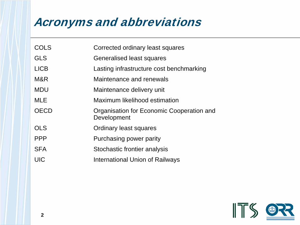
Acronyms and abbreviations
COLS Corrected ordinary least squares
GLS Generalised least squares
LICB Lasting infrastructure cost benchmarking
M&R Maintenance and renewals
MDU Maintenance delivery unit
MLE Maximum likelihood estimation
OECD Organisation for Economic Cooperation and Development
OLS Ordinary least squares
PPP Purchasing power parity
SFA Stochastic frontier analysis
UIC International Union of Railways
3
Introduction (1)
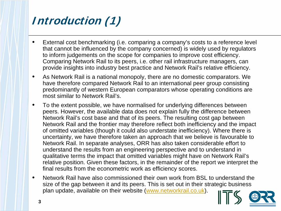
• External cost benchmarking (i.e. comparing a company’s costs to a reference level that cannot be influenced by the company concerned) is widely used by regulators to inform judgements on the scope for companies to improve cost efficiency. Comparing Network Rail to its peers, i.e. other rail infrastructure managers, can provide insights into industry best practice and Network Rail’s relative efficiency.
• As Network Rail is a national monopoly, there are no domestic comparators. We have therefore compared Network Rail to an international peer group consisting predominantly of western European comparators whose operating conditions are most similar to Network Rail’s.
• To the extent possible, we have normalised for underlying differences between peers. However, the available data does not explain fully the difference between Network Rail’s cost base and that of its peers. The resulting cost gap between Network Rail and the frontier may therefore reflect both inefficiency and the impact of omitted variables (though it could also understate inefficiency). Where there is uncertainty, we have therefore taken an approach that we believe is favourable to Network Rail. In separate analyses, ORR has also taken considerable effort to understand the results from an engineering perspective and to understand in qualitative terms the impact that omitted variables might have on Network Rail’s relative position. Given these factors, in the remainder of the report we interpret the final results from the econometric work as efficiency scores.
• Network Rail have also commissioned their own work from BSL to understand the size of the gap between it and its peers. This is set out in their strategic business plan update, available on their website (www.networkrail.co.uk).
4
Introduction (2)
• We have adopted statistical techniques to benchmark Network Rail’s maintenance and renewals (M&R) efficiency. These enable:
The relative efficiency scores to take into account several cost drivers at once, potentially giving a single, more definitive relative performance measure; and
Greater understanding of the impact of key variables on cost. Statistical approaches allow us to determine what the data is telling us about the impact of key variables on cost, for example, the variability of costs with respect to traffic volumes, or the impact of the degree of electrification on costs.
• Assessing unit cost measures alone cannot achieve this. Very different results are often obtained depending on the unit cost chosen (e.g. cost per track km versus cost per train km).
• There are two complementary strands to this work, both of which benchmark total maintenance and renewals spend:
the first, which we have undertaken together with Network Rail, uses the ‘lasting infrastructure cost benchmarking’ (LICB) dataset compiled by the International Union of Railways (UIC). We have shared the work with UIC who intend to evaluate the potential use of the methodology in their work.
The second uses sub-national data from five rail infrastructure managers in Europe and North America that we have collected with the assistance of the comparator companies. We have shared the results with peer companies.
5
Introduction (3)
• This work has been conducted jointly by ORR and the Institute for Transport Studies at Leeds University, in conjunction with Network Rail. Dr Michael Pollitt of Cambridge University has reviewed our analysis.
• We are grateful to the UIC for providing us with access to their dataset, and to Network Rail for working constructively with us. We are also grateful to the infrastructure managers that have worked with us directly to provide the sub-national data. We have shared the results with them.
• However, these outputs, while demonstrating the power of international benchmarking, are specific to the PR08 and our assessment of Network Rail. This document does not report anything about the relative efficiency of any of the comparators to Network Rail.
• In the future we hope that the approach can be developed further to provide a useful tool for the wider rail industry. In the case of the sub-national level benchmarking, we hope to be able to include a greater number of companies in the peer group in future.
International benchmarking using the LICB dataset
7
The dataset: Scope of the dataset
• As part of its own benchmarking analysis, UIC has developed a very useful dataset (the LICB dataset). It currently consists of data for 13 infrastructure companies (or infrastructure divisions within integrated companies), which UIC has collected and refined with its members over the last 11 years. Further information on UIC is available on its website (www.uic.asso.fr).
• The 13 infrastructure companies are Network Rail, OBB (Austria), Infrabel (Belgium), BDK (Denmark), RHK (Finland), DB (Germany), Irish Railways, RS (RFI) (Italy), ProRail (Netherlands), Jernbaneverket (Norway), Refer (Portugal), Banverket (Sweden) and SBB (Switzerland). All of these are publicly owned, with the exception of Network Rail.
• The fact that the dataset contains data for a number of infrastructure managers over a period of time provides a number of advantages over a dataset with only a single year of data. In particular:
The estimate of Network Rail’s relative efficiency is made more robust as the greater number of data points increases the available information and enables more complex modelling techniques to be used; and
It allows us to study the time path of efficiency as well as the absolute levels at a point in time.
8
The dataset: Variables
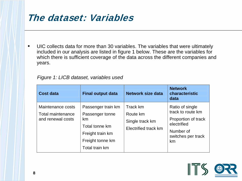
• UIC collects data for more than 30 variables. The variables that were ultimately included in our analysis are listed in figure 1 below. These are the variables for which there is sufficient coverage of the data across the different companies and years.
Figure 1: LICB dataset, variables used
Cost data Final output data Network size data Network characteristic data
Maintenance costs Total maintenance and renewal costs
Passenger train km Passenger tonne km Total tonne km Freight train km Freight tonne km Total train km
Track km Route km Single track km Electrified track km
Ratio of single track to route km Proportion of track electrified Number of switches per track km
9
0
50
100
150
200
250
1996 1998 2000 2002 2004 2006
'000
s co
nsta
nt E
uros Min
Max
Average, exNetwork RailNetwork Rail
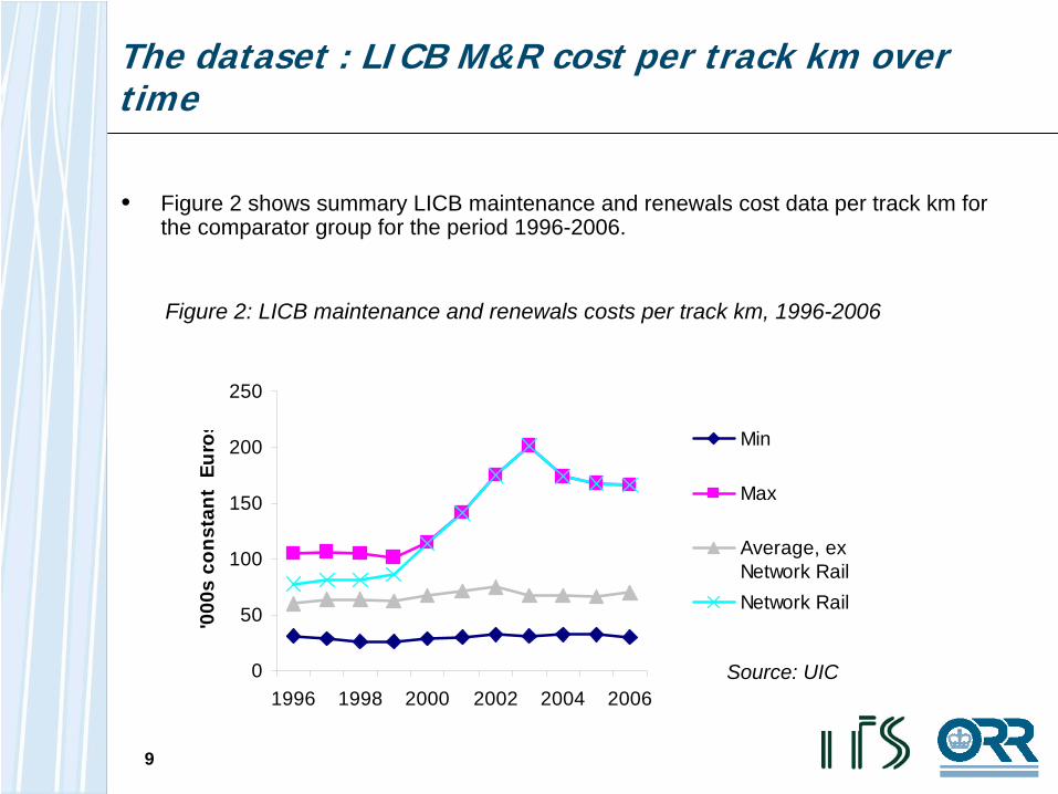
Source: UIC
The dataset : LICB M&R cost per track km over time
Figure 2: LICB maintenance and renewals costs per track km, 1996-2006
• Figure 2 shows summary LICB maintenance and renewals cost data per track km for the comparator group for the period 1996-2006.
10
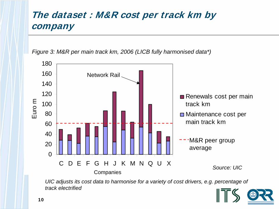
The dataset : M&R cost per track km by company
020406080
100120140160180
C D E F G H J K M N Q U X
Eur
o m
Renewals cost per maintrack kmMaintenance cost permain track km
UIC adjusts its cost data to harmonise for a variety of cost drivers, e.g. percentage of track electrified
Figure 3: M&R per main track km, 2006 (LICB fully harmonised data*)
M&R peer group average
Source: UIC
Network Rail
Companies
11
The dataset: Data cleaning
• We took the LICB dataset largely as given, though we did check for unusually large changes in data values from year to year. We determined whether these changes were justified by changes in other variables correlated to the trend examined and whether the trend appeared to be confirmed by other published sources or data collected. As a result of this analysis, a small number of data points were amended where the evidence strongly suggested that an input error had been made.
• In addition, we made a small number of changes to the data where gaps existed in the dataset (e.g. where data for a variable for a particular company was missing for a single year). Two methodologies for infilling were applied as follows:
For variables for which there were other related variables, with which we would reasonably expect the variable to be correlated, we used the relevant annual growth rate of the related variable to pro-rata the missing observations. This applied to the traffic variables in particular; and
For the physical variables and cost variables for which no clearly correlated variables were available, we used simple interpolation / extrapolation to obtain the relevant observation from the overall trend in that variable.
• The impact of this data cleaning should be small given the approach adopted and that the small number of data points amended.
12
The dataset: Adjusting for PPP
• Cost data were supplied in both local currency and Purchasing Power Parity (PPP) Euros.
• So that we could be sure of the underlying assumptions concerning inflation and the PPP adjustment, we started with the local currency information and used PPP exchange rate data from the OECD to convert the data to a common currency and price level for each year. In this way, we controlled for differences in national price levels (including wages) that affect costs. To control for inflation, the data was then deflated to a common year price level (with German Euros in 2005 as the numeraire). We used these real cost figures in our analysis.
13
Methodology: Benchmark and explanatory variables
• We have benchmarked total M&R costs together. We believe that this is more appropriate than considering maintenance and renewals separately as it means that both the trade-offs between M&R and any accounting differences between countries in the way in which they record maintenance and renewals costs, are taken into account. However, we have also modelled maintenance and renewals costs separately as a crosscheck.
• We have tested a number of cost drivers. Our preferred model considers total maintenance and renewals expenditure as a function of route km, passenger train density, freight train density, the proportion of route that is single track, the proportion of track that is electrified, and time. The single track and electrification variables provide an indication of the complexity of the track and the nature of the assets being maintained / renewed.
14
Methodology: Model formulation
• Based on statistical and other considerations, we determined that the Cobb Douglas function was the most appropriate functional form for the model. In a Cobb Douglas model all variables are in logs as the coefficients represent proportionate changes in cost resulting from proportionate changes in each explanatory variable (the coefficients are known as elasticities).
• Our models were therefore:
Maintenance and renewal costs = f (ROUTE, PASSDR, FRDR, SING, ELEC, TIME, TIME SQUARED) + ERROR
Maintenance costs = f (ROUTE, PASSDR, FRDR, SING, ELEC, TIME, TIME SQUARED) + ERROR
Renewal costs = f (ROUTE, PASSDR, FRDR, SING, ELEC, SWITCH, TIME, TIME SQUARED) + ERROR
where, ROUTE=route-km, PASSDR=passenger train density; FRDR=freight train density; SING=single track-km divided by route-km; ELEC=electrified track-km divided by track-km; SWITCH=number of switches per track km; TIME= time trend
15
Methodology: Analytical approach
• There are a variety of statistical / econometric methods that could be applied. We have tested several approaches:
Pooled models (COLS and stochastic frontier models),
Time invariant panel econometric models, and
Time varying panel econometric models.
• Annex A sets out these methodologies.
• All the methodologies construct an ‘efficiency frontier’, based on the performance of those company’s in the peer group deemed to be most efficient. Any company located on the frontier is considered to be efficient. The relative efficiency of other companies is then determined by their ‘distance’ from this frontier. The further they are from the frontier, the greater is their scope for efficiency catch up.
• As noted in the introduction, we recognise that the distance from the frontier may reflect both inefficiency and the impact of omitted variables. ORR has therefore undertaken analysis in parallel to understand the likely impact of omitted variables in Network Rail’s case. The results of this give us no reason to believe that incorporating omitted variables would be favourable to Network Rail. In constructing our statistical / economic models, we have also taken an approach that is favourable to Network Rail. Given this, in the remainder of this report we interpret the final results from the econometric analysis as ‘efficiency scores’.
16
Methodology: Our preferred approach
• Our preferred approach is a time varying panel model (similar to the model set out in Cuesta 2000), which both recognises the panel structure of the data (i.e. that the data follows 13 firms over time) and allows the pattern of efficiency to vary across firms and time. It is estimated by maximum likelihood methods*.
• This is in contrast to pooled models, which do not recognise the panel structure of the data. In pooled models, the efficiency of each firm is instead assumed to vary randomly over time. This assumption does not appear realistic for this dataset.
• It also contrasts to the time invariant panel models, which recognise the panel structure of the data, but at the cost of assuming that inefficiency is invariant over time. Such an assumption is considered unrealistic, particularly for Network Rail where costs have changed substantially over the eleven years under consideration.
• The approach we have used is also more flexible than the Battese and Coelli (1992) time varying panel model, which is restrictive in the way that efficiency is permitted to vary over time. In particular:
The direction of change in efficiency is the same for all firms and the rankings of all firms is the same in all years; and
It does not permit turning points in efficiency over the period, so that efficiency is either increasing or decreasing for all firms in all time periods.
• All our models have been run in version 9.0 of LIMDEP.* This method is within the class of random effects models (as opposed to fixed effects) and this choice is supported by the Hausman test statistics.
17
Methodology: Steady state adjustment
• Network Rail has asserted that part of the difference between its cost base and that of its peers is due to it renewing assets at a rate greater than the steady state as it continues to redress the backlog built up in the years before the Hatfield derailment.
• ORR is not convinced that Network Rail is out of steady state by the end of the time period considered. However, to ensure that the benchmarking does not penalise Network Rail unfairly for this, we have made an adjustment to Network Rail’s renewal data that assumes their track and signalling renewals volumes are running ahead of steady state even in 2006.
• In particular, we have amended Network Rail’s renewals data so that it is consistent with 2.5% of total track and signalling assets being renewed in each year, implying an average life of 40 years for these assets. This increases the renewals cost data used for Network Rail in the years up to 2000 and reduces it thereafter.
• We have made this adjustment for the total M&R and the renewals only models.
• No such adjustment has been made to the data for other countries. We are therefore assuming that, on average, the leading firms are in steady state.
• We are also assuming that there are constant returns to scale in track and signalling renewals, i.e. that unit costs are constant as volumes increase. This is not an unreasonable assumption but, if anything, is a conservative assumption.
18
Methodology: Explaining ‘the gap’
• We have used a top-down methodology. While this is valuable in identifying any potential efficiency gap between peers, it cannot explain the detailed reasons for the gap.
• ORR has therefore separately undertaken work to confirm whether this gap can be explained, focusing on engineering assessment. It is important to note, however, that it is not the purpose of this work to provide a fully detailed plan to explain the entire gap. The key areas of work relevant to this are:
The lessons learnt from ORR’s visits in 2007 to infrastructure managers in Europe, North America and Australia;
The work carried out by ORR to compare the costs of the GB network with four of the main European comparators (Belgium, Germany, Netherlands, Switzerland) who operate at lower cost than Network Rail.
The BSL study conducted for Network Rail that attempts to explain the gap between implied by the LICB data from a bottom-up perspective; and
The study carried out by RailKonsult for ORR, which examines technologies and working practices used in Europe could help account for the differences in the cost gap between Network Rail and the LICB comparators
• Further details of this work are provided in our draft determination (available on our website: www.rail-reg.gov.uk) and references are provided at the end of this pack.
19
Results: Our preferred model (1)
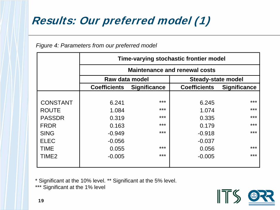
Figure 4: Parameters from our preferred model
* Significant at the 10% level. ** Significant at the 5% level. *** Significant at the 1% level
Coefficients Significance Coefficients Significance
CONSTANT 6.241 *** 6.245 ***ROUTE 1.084 *** 1.074 ***PASSDR 0.319 *** 0.335 ***FRDR 0.163 *** 0.179 ***SING -0.949 *** -0.918 ***ELEC -0.056 -0.037TIME 0.055 *** 0.056 ***TIME2 -0.005 *** -0.005 ***
Time-varying stochastic frontier model
Raw data model Steady-state modelMaintenance and renewal costs
20
0.4
0.5
0.6
0.7
0.8
0.9
1.0
1.1
1996
1998
2000
2002
2004
2006
NR
sco
res
vs U
Q NR inc. steady state
adjustmentNR ex. steady stateadjustmentUpper quartile
Results: Our preferred model (2)
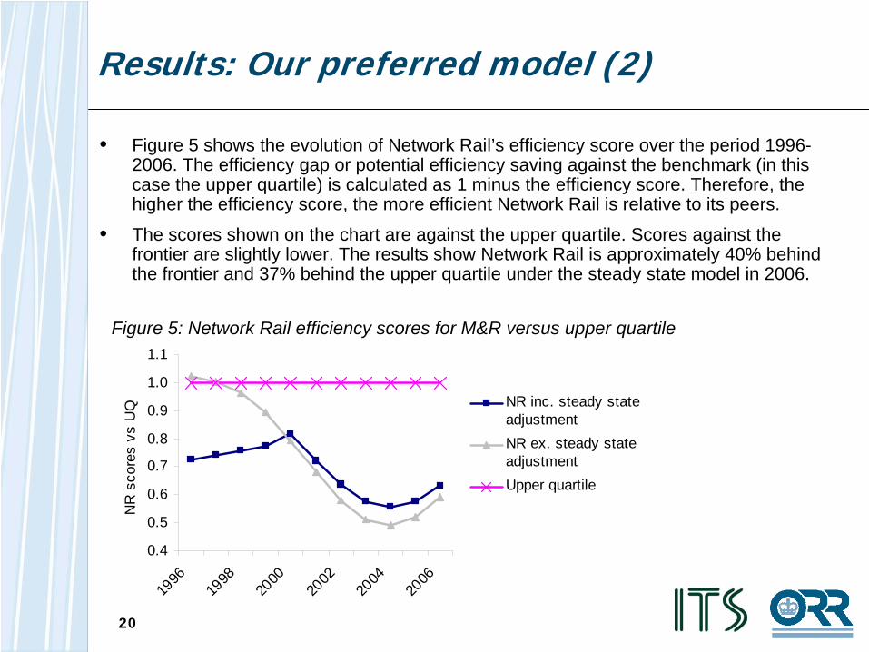
• Figure 5 shows the evolution of Network Rail’s efficiency score over the period 1996- 2006. The efficiency gap or potential efficiency saving against the benchmark (in this case the upper quartile) is calculated as 1 minus the efficiency score. Therefore, the higher the efficiency score, the more efficient Network Rail is relative to its peers.
• The scores shown on the chart are against the upper quartile. Scores against the frontier are slightly lower. The results show Network Rail is approximately 40% behind the frontier and 37% behind the upper quartile under the steady state model in 2006.
Figure 5: Network Rail efficiency scores for M&R versus upper quartile
21
• The test statistics strongly indicate the presence of inefficiency effects, i.e. that there are differences in the efficiency of peer companies.
• The deterioration and subsequent recovery in Network Rail’s relative efficiency after 2000 are also statistically significant. Network Rail’s relative efficiency has declined markedly since 2000, even taking into account the steady state adjustment. However, it has started to recover since 2004, which is to be expected given the sizeable efficiency improvements the company has achieved in the first half of CP3.
• As expected, the steady state adjustment improves Network Rail’s efficiency scores in the years after the Hatfield derailment.
• The parameter estimates appear to be well behaved, in that their sign and magnitude make sense from an engineering perspective and are in line with the results of previous econometric work. The sign of the coefficient on the electrification variable is potentially ambiguous. On the one hand, more electrification assets should require higher M&R activity. On the other, it is possible that the electrification variable is acting as a proxy for other network characteristics.
• The parameter estimates are also statistically significant. The exception to this is the electrification coefficient. Removing this variable either has little impact on Network Rail’s efficiency score or reduces it (implying greater relative inefficiency) depending on the model used. However, we prefer to retain it in the model, based on theoretical considerations - that is, we expect this variable to impact on costs – and the variable is statistically significant in the maintenance only model. It is possible that its effect in the M&R model is being obscured by its correlation with some of the other explanatory variables.
Results: Our preferred model (3)
22
Results: Sensitivity analysis
• We have tested the sensitivity of our results to the choice of functional form and the methodology used. We have selected the simpler Cobb-Douglas form (though with a squared term on for the time trend variable) either because the choice of functional form had little impact on the results, or because there were good reasons for rejecting the more complex translog form (in terms of the credibility of the parameter estimates).
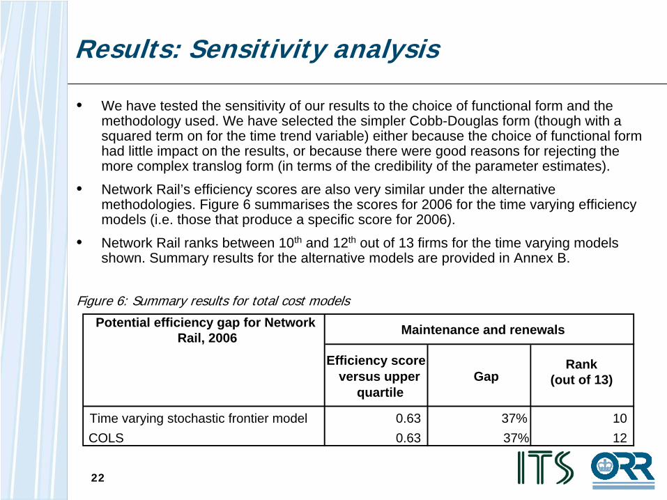
• Network Rail’s efficiency scores are also very similar under the alternative methodologies. Figure 6 summarises the scores for 2006 for the time varying efficiency models (i.e. those that produce a specific score for 2006).
• Network Rail ranks between 10th and 12th out of 13 firms for the time varying models shown. Summary results for the alternative models are provided in Annex B.
Figure 6: Summary results for total cost models
Potential efficiency gap for Network Rail, 2006
Efficiency score versus upper
quartileGap
Rank(out of 13)
Time varying stochastic frontier model 0.63 37% 10COLS 0.63 37% 12
Maintenance and renewals
2323
Conclusion
• We believe that the statistical models that we have produced are robust, making sense from both econometric and engineering perspectives. The results are also robust to changes in the methodology and small changes in the dataset.
• As noted earlier, while we recognise the difficulties associated with benchmarking, where there are uncertainties we have taken an approach that we believe is favourable to Network Rail. The parallel qualitative and engineering based work also supports the results from our econometric analysis.
• Our preferred model suggests Network Rail is 37% less efficient in maintenance and renewals than the leading group of countries in the peer group (the upper quartile).
• We consider that our approach is generous to Network Rail (i.e. if anything, it underestimates the potential for Network Rail to improve its efficiency) as:
We have benchmarked Network Rail against the upper quartile not the frontier;We have sought to ensure that our approach takes account of uncertainty, and therefore avoids comparing Network Rail’s performance to a company exhibiting particularly low cost in a particular year; andThe peer group does not necessarily reflect best practice. For instance, the peer group consists of public sector owned companies. Work conducted for us by NERA suggests that publicly owned enterprises generally are likely to be less efficient than those that are privatised. Given Network Rail’s aim of becoming a ‘world class’ company, its aim should arguably be to exceed the levels of efficiency implied by this peer group.

Regional international benchmarking
2525
Introduction
• During the period Autumn 2006 to Autumn 2007 we held discussions with and collected data from a number of rail companies with a view to carrying out an international benchmarking study.
• Whilst demonstrating the power of international benchmarking, the results in this report are specific to Network Rail and PR08. This document does not report anything about the relative efficiency of any of the comparator railways.
• We have separately provided to each of the comparator railways the results for their own company.
• We are grateful to the companies that have worked with us to provide data. Going forward, we hope that the approach can provide a useful tool for the wider rail industry, potentially incorporating a greater number of comparator companies.
2626
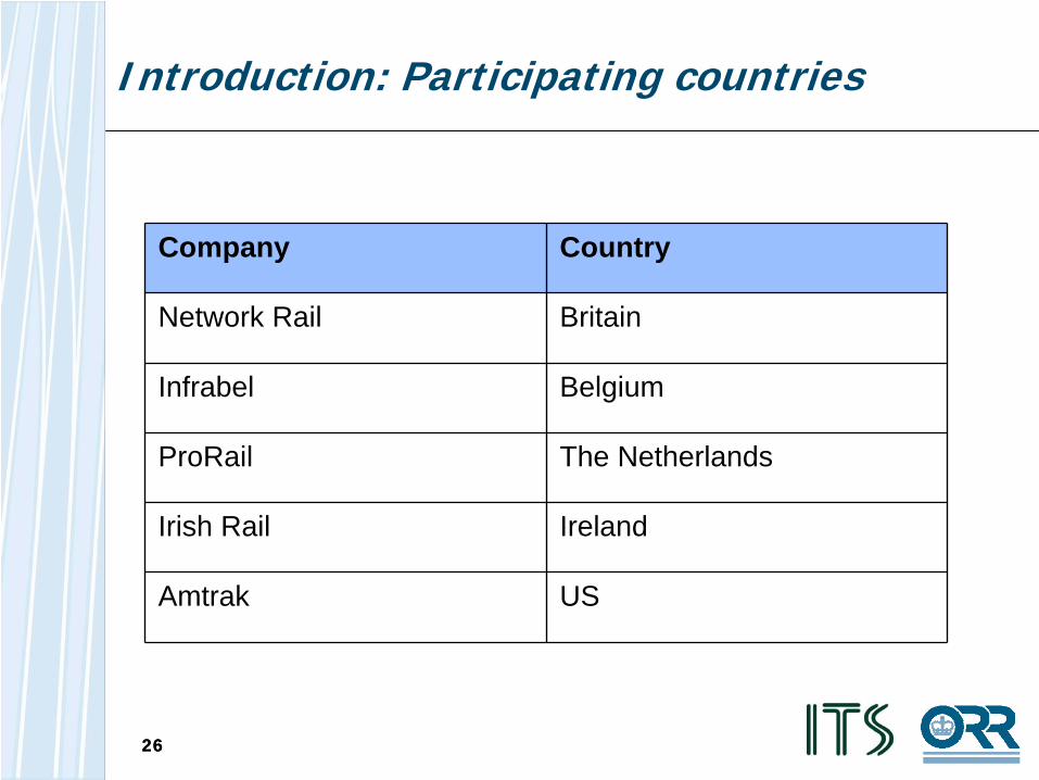
Introduction: Participating countries
Company Country
Network Rail Britain
Infrabel Belgium
ProRail The Netherlands
Irish Rail Ireland
Amtrak US
27
• We obtained data directly from the 5 participating countries. The data collection was undertaken during 2006 and 2007 via face to face meetings with comparator companies and conference calls.
• The data was provided for a number of geographical areas in each country and, for some countries, for a number of years. The total number of observations (areas within countries and over time) is 52.
• The cost data for Network Rail was provided for the year 2005/06 (2006/07 for track renewals) at maintenance delivery unit (MDU) level. There are 51 MDUs covering the whole of the GB network.
• However, not all costs are allocated to the MDU level. Instead, a significant proportion (33%) are only allocated to the Area level. There are 18 Areas covering the whole of the GB network.
• To fit with the definitions of costs from other countries, for the purpose of our analysis, we aggregated the MDU level data to Area level.
• The data was converted to a common currency using PPP exchange rates (and has also been converted into constant prices).
27
The dataset: Scope of the dataset
2828
The dataset: Issues arising
• The advantages of the data set (which will increase over time following iterations of further data collection and analysis)
Reliable data source. As noted above, we collected the data directly from the companies and so it is fully traceable.
We can potentially acquire a set of consistent quality and capability variables for all countries
Potentially there are many observations for a relatively small time period –yielding benefits to modelling precision
• We experienced some data issues, which we expect to diminish over time following iterations of further data collection and analysis:
It was difficult to get the same measures of quality reported for all railways (at present only the proportion of track length electrified is available); and
At present we only have a single year’s data for Network Rail, although we have data for up to 5 years for some companies. Having multi-year data for at least some comparators is preferable to just a single year cross section but does, by construction, limit us to considering time invariant models only.
2929
Methodology: Benchmark and explanatory variables
• We considered two cost categories to analyse:
Total maintenance cost only
Total maintenance and track renewal cost
• We then had two measures of traffic to consider for each cost category which we analysed separately:
Total tonnage density (tonne km per track km; TTKM)
Passenger tonnage density (PTKM) and Freight tonnage density (FTKM)
• We also included proportion of track electrified as a variable to capture some of the network characteristics / quality differences between networks.
3030
Methodology: Model formulation
• We determined the best functional form through statistical testing for each of the cost/traffic combinations. After considering a range of functions we determined that the Cobb Douglas function (shown in the next slide) was the most appropriate for all cost/traffic combinations.
• In a Cobb Douglas model all variables* are in logs as the coefficients represent proportionate changes in cost resulting from proportionate changes in each explanatory variable (the coefficients are known as elasticities).
• Our models were therefore:
Cost (maintenance or maintenance plus renewals cost) = f (TRACK, PTKM, FTKM, PROELECT) + ERROR
Cost (maintenance or maintenance plus renewals cost) = f (TRACK, TTKM, PROELECT) + ERROR
where, TRACK=track-km, PTKM=passenger tonnage density; FTKM=freight tonnage density; TTKM=total tonnage density; PROELECT=electrified track-km divided by track-km
No time trend is included, as for some companies (including Network Rail) there is only a single year’s data.
* Except proportion of track electrified, which is not logged. Instead we enter this in untransformed form. The coefficient represents a growth rate.
3131
Methodology: Analytical approach
• There are a variety of statistical methods that cold be applied. We have tested several approaches:
Pooled models: Corrected ordinary least squares (COLS) and pooled stochastic frontier analysis; and
Stochastic Frontier ‘Panel’ models.
• The choice between models is similar to that faced in the analysis of the UIC data described above. In this case, the pooled approaches allow each region to have different efficiency scores, but do not recognise the structure of the data (that each region is actually part of a whole railway).
• The panel specifications assume the same efficiency score for each region within a given railway. They ignore any internal variation in efficiency, but recognise the structure of the data.
• Annex A provides more detail on the various methodologies.
3232
Methodology: Our preferred approach
• There is a trade-off when selecting the preferred method. Following a thorough review of both modelling approaches, we prefer the panel approach. This is due to:
The robustness of the parameter estimates in the panel models,An understanding that the Network Rail Areas do not have management autonomy (unlike the MDUs) and so there is not such a strong need to account for autonomy, andThe fact that we are interested in determining differences in efficiency at the overall company level in this analysis.
• As is usual in the efficiency measurement literature, we considered three panel approaches:
Fixed effects modellingRandom effects modelling estimated first by generalised least squares (GLS) and second by maximum likelihood estimation (MLE).
• We tested between fixed and (GLS) random effects using the Hausman test. The results of the tests suggested that the random effects models were superior.
• The results of the two random effects estimation procedures do not differ substantially, and so we present only the maximum likelihood model results.
• Note that as we only have a single year’s data for some companies (including Network Rail), all of the panel models are time invariant efficiency models.
3333
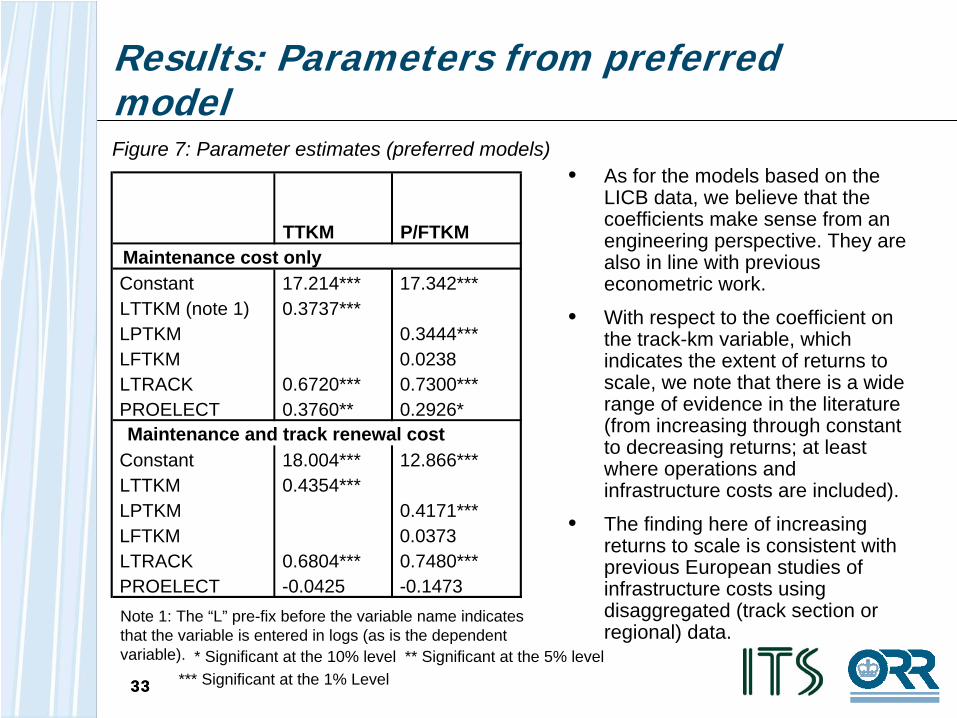
Results: Parameters from preferred model
• As for the models based on the LICB data, we believe that the coefficients make sense from an engineering perspective. They are also in line with previous econometric work.
• With respect to the coefficient on the track-km variable, which indicates the extent of returns to scale, we note that there is a wide range of evidence in the literature (from increasing through constant to decreasing returns; at least where operations and infrastructure costs are included).
• The finding here of increasing returns to scale is consistent with previous European studies of infrastructure costs using disaggregated (track section or regional) data.
Figure 7: Parameter estimates (preferred models)
* Significant at the 10% level ** Significant at the 5% level *** Significant at the 1% Level
TTKM P/FTKMMaintenance cost onlyConstant 17.214*** 17.342***LTTKM (note 1) 0.3737***LPTKM 0.3444***LFTKM 0.0238LTRACK 0.6720*** 0.7300***PROELECT 0.3760** 0.2926*Maintenance and track renewal cost
Constant 18.004*** 12.866***LTTKM 0.4354***LPTKM 0.4171***LFTKM 0.0373LTRACK 0.6804*** 0.7480***PROELECT -0.0425 -0.1473Note 1: The “L” pre-fix before the variable name indicates that the variable is entered in logs (as is the dependent variable).
3434
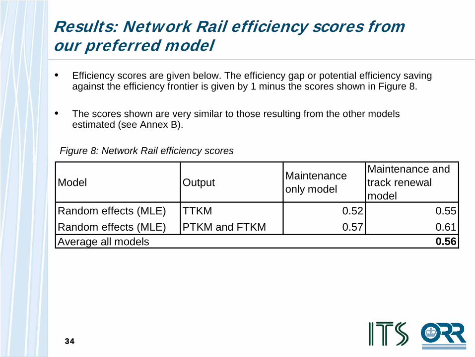
Results: Network Rail efficiency scores from our preferred model
• Efficiency scores are given below. The efficiency gap or potential efficiency saving against the efficiency frontier is given by 1 minus the scores shown in Figure 8.
• The scores shown are very similar to those resulting from the other models estimated (see Annex B).
Figure 8: Network Rail efficiency scores
Model Output Maintenance only model
Maintenance and track renewal model
Random effects (MLE) TTKM 0.52 0.55Random effects (MLE) PTKM and FTKM 0.57 0.61Average all models 0.56
3535
Results: comments on the results
• The preferred models produce generally sensible parameter estimates in that they are consistent with other studies and with engineering judgement.
• The preferred models show the following:Network Rail is ranked 4th out of 5 in all the preferred panel random effects models;Using these unadjusted scores, Network Rail appears to be about 56% efficient based on our preferred models (an average of the random effects efficiency scores);Taken at face value, this would imply that if Network Rail could exploit the frontier best practice then it could cut costs by 44%;It should be borne in mind however that these are ‘raw’ scores and simply represent the gap between Network Rail and the frontier. There may be reasons other than inefficiency for this gap;However, we have no reason to believe that any variables omitted are producing unfavourable cost conditions for Network Rail. And the effect could work in other direction, meaning that the company’s efficiency gap is larger than that implied by the model;The results are consistent with the results based on the LICB data, which puts Network Rail’s gap against the frontier at approximately 40% (after the steady-state adjustment) and 43% (before the steady-state adjustment).
3636
Conclusions
• Preliminary analysis of this data set has yielded a set of reasonable models
• Overall the results support those from the study of the UIC LICB dataset
• For the total maintenance and total maintenance and track renewal cost categories, the various models produce very similar efficiency scores, efficiency rankings and parameter estimates
• We expect that future development of the dataset and methodology will further strengthen the robustness of the analysis.
Annex A: Methodological annex
38
Annex A: Methodological overview (1)
• In our analysis, we estimate a cost frontier model and consider deviations from the frontier as inefficiency. There will be other factors influencing the cost variation between comparators that cannot be included in the model (due to a lack of data). Part of any ‘efficiency gap’ identified by our models may therefore reflect omitted variables, thus overstating the efficiency variation within the sample. However, our models may also underestimate the efficiency gap for individual companies depending on the direction of influence of omitted variables. As noted earlier, in reaching its conclusions on Network Rail’s efficiency position, ORR has supplemented the results of the econometric work with other evidence. In the remainder of this annex we use the term inefficiency in our discussion of the different models in respect of Network Rail. This document does not report anything about the relative efficiency of any of the comparators to Network Rail.
39
Annex A: Methodological overview (2)
• We consider two types of frontier:
A deterministic frontier, where all unexplained variation in cost is deemed to be indicative of inefficiency; and
A stochastic frontier, where there is explicit consideration that unexplained deviation maybe the result of random noise as well as inefficiency.
• The models can be summarised as:
• We include the traffic variables as densities (e.g. tonne-km divided by track-km) as it seems reasonable to consider the effect of increasing usage on a fixed network rather than allowing the network size to vary. We also note that in the double log functional form finally adopted for the study, apart from ex post transformations of coefficients, it makes no difference to the estimation results how these variables are entered.
Cost = f(traffic density, network length, infrastructure quality and capability variables) + error
40
Annex A: Functional form (1)
• We consider four candidate functional forms :
The linear form: all variables in levels as they appear within the function above;
The quadratic form: as for the linear function but with squared and cross terms for the traffic and track length variables;
Cobb Douglas: as for the linear function but with the dependent and explanatory variables entered in natural logarithms; and
Translog: as for the Cobb Douglas but with square and cross terms for the traffic and track length variables.
• The testing strategy is first to test between the quadratic and Translog forms as these nest (that is subject to linear restrictions they contain) the linear and Cobb Douglas forms respectively. Second a test of the linear restrictions regarding whether the restricted forms are rejected is undertaken.
• It is difficult to test between functional forms where the dependent variables are different. In the linear and quadratic forms the dependent variable is cost while in the Cobb Douglas and Translog the dependent variable is ln (cost). Ultimately the problem arises because the explanatory variables are ‘explaining’ different things, either cost or the log of cost.
41
Annex A: Functional form (2)
• We test between the quadratic form and Translog form by a variant of the Box Cox Test proposed by Zarembka (1968). Details of this test can be found in Dougherty (1992). This test transforms the dependent variables in such away that the fits of the models can be compared and then a test can be conducted to determine whether one is statistically better than the other. Note that this test uses the residual sum of squares so we considered the ordinary least squares (OLS) model only. The result of the test is that for both output specifications and cost variables, the Translog model has superior fit to the quadratic model and this is found to be statistically superior such that we can reject the Quadratic model in favour of the Translog.
• The restrictions for the Cobb Douglas were then tested on a model by model basis depending on the error specification to which we now turn.
42
Annex A: Error specification (1)
• When conducting efficiency analysis, the appropriate specification of the error is essential as the error yields the information about firm inefficiency. We consider several specifications and each approach is discussed below.
Deterministic frontier – Corrected ordinary least squares (COLS)
• COLS is the simplest approach. It assumes that any unexplained variation in (ln)cost is due to inefficiency. In this case we estimate the model using a two stage approach.
First, we estimate the model using the standard ordinary least squares regression method.
Second, we shift the resulting cost line down so that no points are below the line and (at least) one point is on the line.
• This constrains the residuals to be either zero (on the line) or greater than zero (above the line), which is required as inefficiency can not be negative.
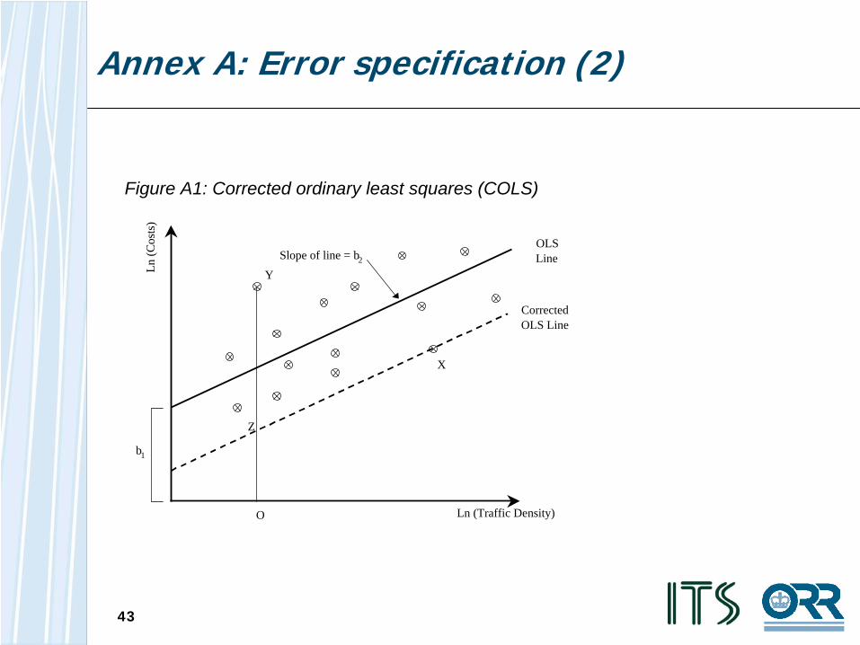
• In figure A1 we show a regression of ln (costs) on a single variable (ln (traffic density)). OLS yields the solid line. We then shift the line downwards so that all of the observations are on or above the line. The line is now a frontier. In this example, observation X defines the frontier. Observation Y is inefficient as it is above the frontier and its efficiency is measured based on the distances OZ and OY
43
Annex A: Error specification (2)
Figure A1: Corrected ordinary least squares (COLS)
Ln (C
osts
)
Ln (Traffic Density)
OLS Line
Corrected OLS Line
b1
Slope of line = b2
X
Y
O
Z
44
Annex A: Error specification (3)
• The limitation of the COLS approach is ultimately its simplicity. In particular, interpreting all unexplained variation in ln(cost) as inefficiency is misleading since inefficiency is only one of a number of factors that can account for deviation from the fitted relationship, other factors being measurement error and unobservable factors, for example. It is likely that firm inefficiency scores will be inflated given that the COLS frontier is fit through the point with minimum residual, which is likely to have a negative impact from other factors.
• In regulatory contexts it is often felt necessary to mitigate for this limitation by only shifting the OLS line down to the position of the 75th percentile residual (upper quartile). In this case, not all points will be above or on the line, with points below the frontier deemed to be ‘super-efficient’ as a result of noise in the data.
45
Annex A: Error specification (4)
Pooled stochastic frontier model
• More advanced efficiency models have been proposed. These allow for the error to be composed of (at least) two components; inefficiency and random error. We first consider a pooled stochastic frontier model.
• This model was first proposed independently by Aigner et al (1977) and Meeusen and van den Broeck (1977). They separated the overall error into two components each with a different distributional form. The inefficiency error has a strictly positive distribution (e.g. half-normal distribution) and the other component representing random noise has a normal distribution. This model is estimated using the method of maximum likelihood. Following estimation, firm specific estimates of inefficiency can be calculated using the method original proposed by Jondrow et al.
• In this framework, we can distinguish between a deterministic frontier and a stochastic frontier. The deterministic frontier is the minimum cost point for the firm conditioned on the measured variables in the estimated cost function. The stochastic frontier is the sum of the deterministic frontier and the realisation of the random noise error for the specific firm. This represents the minimum cost attainable by the firm after according for both measured and unmeasured factors. This maybe above or below the deterministic frontier depending on the influence of the unobserved factors. Importantly, each firm will have a different stochastic frontier.
46
Annex A: Error specification (5)
Panel stochastic frontier models
• The datasets used in this analysis have multiple observations for individual railways. In such circumstances the data set is know as a panel dataset. When dealing with a panel dataset a decision has to be made about how to deal with inefficiency for each firm in terms of its behaviour over each observation. When a panel consists of multiple observations of a firm over time there are usually three options:
Treat each observation in the data set as an independent observation (i.e. ignore the panel structure) and assume that inefficiency is distributed independently of each observation. Thus the data is pooled and we have the model outlined in the previous sub-section;
Assume that all observations for each particular firm have the same inefficiency; or
Assume that all observations for each particular firm have inefficiency which can vary through time but this variation is determined by a deterministic function. This relaxes the assumption of independence between observations for each firm.
47
Annex A: Error specification (6)
• For the analysis based on the UIC data, our preferred model is based on the third option. Specifically, it is based on the model developed by Cuesta (2000)*, and it both recognises the panel structure of the data (i.e. that the data follows 13 firms over time) and allows the pattern of efficiency to vary across firms and time (in potentially different directions and to different extents).
• However, for comparative purposes, in this presentation we compare the results against the COLS model. Whilst the COLS model does not recognise the structure of the data, it nevertheless allows efficiency to vary over time in a very flexible way and is widely used by economic regulators.
• For the purpose of this analysis time invariant efficiency models – that do not allow efficiency to vary over time, and thus produce a single score for each company – are not considered appropriate, given the substantial changes in costs experienced by Network Rail (and indeed other companies) over the period covered by the dataset.
* It is a more general version of Cuesta (2000) that also allows the direction of efficiency change to alter during the period. See Kumbhakar and Lovell (2000), pages 110-113.
48
Annex A: Error specification (7)
• The dataset for the regional benchmarking has multiple observations by sub- company and (in some cases) by time. Thus there are three other permutations to consider:
Allow variation in inefficiency over time and over sub-companies within each firm;
Allow variation in inefficiency over time but not over sub-companies within each firm; or
Allow variation in inefficiency over sub-companies but not through time.
• For the panel modelling in the regional benchmarking study we choose to assume that all observations (both sub-company or over time variation) for a particular firm have the same inefficiency. We consider this reasonable for the following reasons:
Only one railway has supplied data for more than 2 years. It therefore seems reasonable to apply time invariant inefficiency methods;
Regarding variation by sub-company, the two candidates are to assume independence between sub-company units or assume inefficiency does not vary between sub-companies; and
We choose to the latter because we wish to identify systematic inefficiency differences across railways.
49
Annex A: Error specification (8)
• This model can be estimated by three methods:
The first is, as with the pooled stochastic frontier model, using maximum likelihood. This imposes specific distributions on each of the error components.
The second is still, like the first, a random effects framework, but this time estimated by generalised least squares (GLS). This does not require such stringent distributional assumptions on the two error components but at the cost of some estimation precision.
Finally we have a fixed effects framework estimated by the least squares dummy variable method. This relaxes the distributional assumptions further, allowing for correlation between the deterministic frontier and the inefficiency terms. The cost is a further loss of estimation precision relative to the other two estimators. We can test between the fixed effects and GLS random effects model using the Hausman test.
• For the regional benchmarking, there are arguments for and against adopting the panel approach versus adopting the pooled approach. This has to do with the need to capture differences in the performance of individual regions in each country (reflected in the pooled approach) against the need to recognise that regions in the same country will have an element of common performance resulting from firm wide management. On balance, following a thorough review of both modelling approaches we prefer the panel modelling approach.
Annex B: Summary results for alternative models
5151
Contents• This annex contains some further information on other models run for both the LICB
and regional international datasets that are not shown in the main body of the report.
5252
Other model results: LICB dataset• As noted above a range of models were run as part of this work. The main body of
the report shows the results of the two time varying efficiency models (COLS) and the model based on a generalisation of Cuesta (2000).
• Other models were run and the results are not shown in the main body of the report, either because they were not well behaved (i.e. stochastic frontier models that assume the efficiency of each company varies over time in a random way) or on the grounds that the model assumptions were not considered appropriate for the present purpose.
• The latter category includes time invariant efficiency models, which are particularly restrictive in this context given the considerable changes in cost that have occurred during this period for Network Rail. In particular, such models produce a single score for Network Rail covering the whole period 1996-2006, whereas we are interested in Network Rails efficiency in 2006 (and indeed to the end of CP3).
• However, we note that the time invariant (random effects: GLS) model produces an efficiency score against the frontier of 0.60 (after steady-state adjustment) for M&R – the same as that produced by our preferred model.
• The next three slides show the results from the maintenance only and renewals only models based on the LICB data. The final slide of this Annex shows the results of the various models run on the regional international dataset.
5353
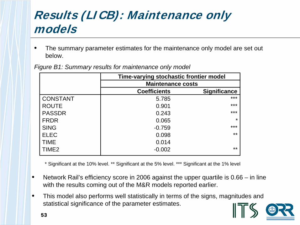
Results (LICB): Maintenance only models• The summary parameter estimates for the maintenance only model are set out
below.
Figure B1: Summary results for maintenance only model
• Network Rail’s efficiency score in 2006 against the upper quartile is 0.66 – in line with the results coming out of the M&R models reported earlier.
• This model also performs well statistically in terms of the signs, magnitudes and statistical significance of the parameter estimates.
* Significant at the 10% level. ** Significant at the 5% level. *** Significant at the 1% level
Coefficients SignificanceCONSTANT 5.785 ***ROUTE 0.901 ***PASSDR 0.243 ***FRDR 0.065 *SING -0.759 ***ELEC 0.098 **TIME 0.014TIME2 -0.002 **
Time-varying stochastic frontier modelMaintenance costs
5454
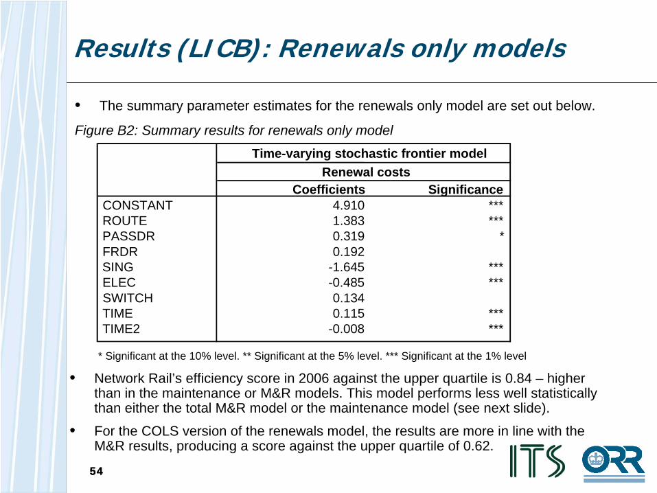
Results (LICB): Renewals only models
• The summary parameter estimates for the renewals only model are set out below.
Figure B2: Summary results for renewals only model
• Network Rail’s efficiency score in 2006 against the upper quartile is 0.84 – higher than in the maintenance or M&R models. This model performs less well statistically than either the total M&R model or the maintenance model (see next slide).
• For the COLS version of the renewals model, the results are more in line with the M&R results, producing a score against the upper quartile of 0.62.
* Significant at the 10% level. ** Significant at the 5% level. *** Significant at the 1% level
Coefficients SignificanceCONSTANT 4.910 ***ROUTE 1.383 ***PASSDR 0.319 *FRDR 0.192SING -1.645 ***ELEC -0.485 ***SWITCH 0.134TIME 0.115 ***TIME2 -0.008 ***
Time-varying stochastic frontier modelRenewal costs
5555
Results: comments on the renewals only models• The renewals only model performs less well statistically than either the total M&R
model or the maintenance model. This is to be expected as renewals are more lumpy than maintenance and, hence, renewals costs are harder to model.
• In particular, the coefficient on the route-km variable (at 1.38) is higher than might be expected based on the received literature (indicating substantial diseconomies of scale), given that the cost base here only includes infrastructure costs.
• The electrification variable takes a negative sign (and is statistically significant). It may be that this variable is picking up the effects of other quality factors that are correlated with electrification, for example age. The magnitude of the coefficient suggests that costs fall quickly with increased electrification. If the electrification variable is dropped, Network Rail’s efficiency score falls substantially.
• It should also be noted that for Network Rail the model suggests that the company’s efficiency score is deteriorating throughout CP3, which is unexpected. There is also disagreement across method here, since the COLS version produces a much lower efficiency score for Network Rail against the upper quartile of 0.62.
• We note that the scores for Network Rail based on the M&R model are lower than those implied by either the maintenance or the renewals models. This partly reflects the problems of modelling the cost categories separately (particularly renewals).
• We therefore base our results on the M&R models which, as noted earlier, are also preferred owing to the need to take account of trade-offs in maintenance and renewal activity and any accounting differences concerning the boundary between maintenance and renewal costs.
5656
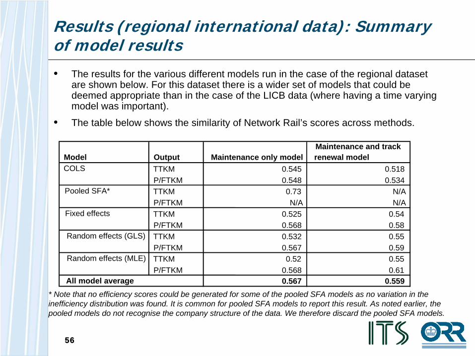
Results (regional international data): Summary of model results
* Note that no efficiency scores could be generated for some of the pooled SFA models as no variation in the inefficiency distribution was found. It is common for pooled SFA models to report this result. As noted earlier, the pooled models do not recognise the company structure of the data. We therefore discard the pooled SFA models.
Model Output Maintenance only modelMaintenance and track renewal model
TTKM 0.545 0.518P/FTKM 0.548 0.534TTKM 0.73 N/AP/FTKM N/A N/ATTKM 0.525 0.54P/FTKM 0.568 0.58TTKM 0.532 0.55P/FTKM 0.567 0.59TTKM 0.52 0.55P/FTKM 0.568 0.61
0.567 0.559
Random effects (GLS)
Random effects (MLE)
All model average
COLS
Pooled SFA*
Fixed effects
• The results for the various different models run in the case of the regional dataset are shown below. For this dataset there is a wider set of models that could be deemed appropriate than in the case of the LICB data (where having a time varying model was important).
• The table below shows the similarity of Network Rail’s scores across methods.
References
58
References (1)
• Aigner, D.J., Lovell, C.A.K, and Schmidt, P. (1977), Formulation and Estimation of Stochastic Frontier Production Function Models, Journal of Econometrics, vol. 6 (1), pp 21-37
• Battese, G.E. and Coelli, T.J. (1992), ‘Frontier Production Functions and the Efficiencies of Indian Farms Using Panel Data from ICRISAT’s Village Level Studies’, Journal of Quantitative Economics, vol. 5, pp. 327-348.
• BSL (2008), Rail Infrastructure Cost Benchmarking: Brief LICB-gap analysis and cost driver assessment. This may be accessed on Network Rail’s website at http://www.networkrail.co.uk/browse%20documents/StrategicBusinessPlan/Update/ Cost%20benchmarking%20assessment%20(BSL).pdf
• Cuesta, R. A. (2000). ‘A Production Model with Firm-Specific Temporal Variation in Technical Inefficiency: With Application to Spanish Dairy Farms’ Journal of Productivity Analysis, 13, pp. 139-158.
• Dougherty, C (1992), Introduction to Econometrics, Oxford University Press
• Jondrow, J., I. Materov, K. Lovell and P. Schmidt (1982), On the Estimation of Technical Inefficiency in the Stochastic Frontier Production Function Model, Journal of Econometrics, 19, 2/3, pp. 233-238
• Kumbhakar, S.C. and Lovell, C.A.K. (2000), Stochastic Frontier Analysis, Cambridge University Press, Cambridge UK.
59
References (2)
• Meeusen, W. and van Den Broeck, J. (1977), Efficiency Estimation from Cobb- Douglas Production Functions with Composed Error, International Economic Review, vol. 18 (2), pp. 435-444
• NERA (2006), Corporate Form, Financial Guarantees, and Efficiency Performance: Expectations and Evidence. This is available at http://www.rail- reg.gov.uk/upload/pdf/pr08-isbp-nera.pdf.
• Zarembka, P (1968), Functional form in demand for money. Journal of the American Statistical Association 63(322): 502-511