International Economics IIncreasing Returns to Scale (The Krugman Model)

Tomás Rodríguez Martínez

Universitat Pompeu Fabra and BGSE

1 / 40

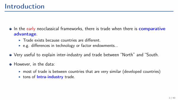
Introduction

In the early neoclassical frameworks, there is trade when there is comparativeadvantage.

I Trade exists because countries are different.I e.g. differences in technology or factor endowments...

Very useful to explain inter-industry and trade between “North” and “South.

However, in the data:I most of trade is between countries that are very similar (developed countries)I tons of Intra-industry trade.

2 / 40

Introduction

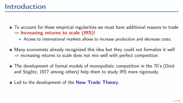
To account for these empirical regularities we must have additional reasons to trade⇒ Increasing returns to scale (IRS)!

I Access to international markets allows to increase production and decrease costs.

Many economists already recognized this idea but they could not formalize it well⇒ increasing returns to scale does not mix well with perfect competition.

The development of formal models of monopolistic competition in the 70’s (Dixitand Stiglitz, 1977 among others) help them to study IRS more rigorously.

Led to the development of the New Trade Theory.

3 / 40

Introduction

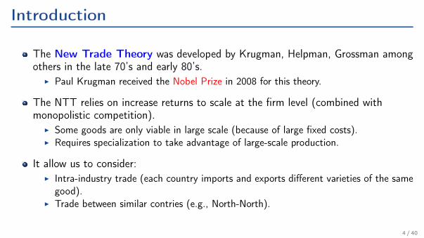
The New Trade Theory was developed by Krugman, Helpman, Grossman amongothers in the late 70’s and early 80’s.

I Paul Krugman received the Nobel Prize in 2008 for this theory.

The NTT relies on increase returns to scale at the firm level (combined withmonopolistic competition).

I Some goods are only viable in large scale (because of large fixed costs).I Requires specialization to take advantage of large-scale production.

It allow us to consider:I Intra-industry trade (each country imports and exports different varieties of the same

good).I Trade between similar contries (e.g., North-North).

4 / 40

Introduction

Modeling Increasing Returns to Scale

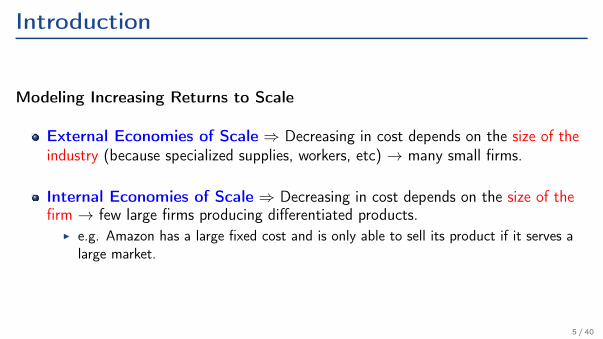
External Economies of Scale ⇒ Decreasing in cost depends on the size of theindustry (because specialized supplies, workers, etc) → many small firms.

Internal Economies of Scale ⇒ Decreasing in cost depends on the size of thefirm → few large firms producing differentiated products.

I e.g. Amazon has a large fixed cost and is only able to sell its product if it serves alarge market.

5 / 40

IRS and Differentiated Goods: Intuition

Consider differentiated goods within a sector:I e.g., iPhone and Galaxy S are 2 varieties perceived as imperfect substitutes

Internal economies of scale imply:I Each variety is cheaper if production is concentrated in one large firmI Apple is located in one country (US) and Samsung possibly in another (Korea)

In both countries, some prefer Apple and some SamsungTrade allows both varieties to be sold in both countriesGains:

I Americans (Koreans) preferring Samsung (Apple) are happier.I "competition" with foreign variety reduces the price of both.

6 / 40

Introduction

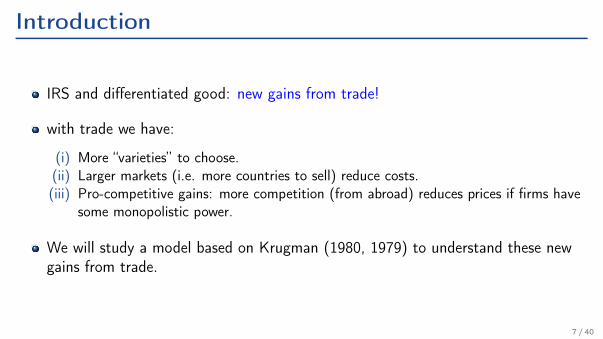
IRS and differentiated good: new gains from trade!

with trade we have:

(i) More “varieties” to choose.(ii) Larger markets (i.e. more countries to sell) reduce costs.(iii) Pro-competitive gains: more competition (from abroad) reduces prices if firms have

some monopolistic power.

We will study a model based on Krugman (1980, 1979) to understand these newgains from trade.

7 / 40

Outline

1. Increasing Returns and Monopolistic Competition

2. Open Economy

3. Pro-Competitive GFT

4. Empirical Evidence

8 / 40

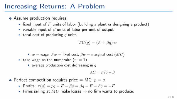
Increasing Returns: A Problem

Assume production requires:I fixed input of F units of labor (building a plant or designing a product)I variable input of β units of labor per unit of outputI total cost of producing q units:

TC(q) = (F + βq)w

F w = wage; Fw = fixed cost; βw = marginal cost (MC)I take wage as the numeraire (w = 1)

F average production cost decreasing in q

AC = F/q + β

Perfect competition requires price = MC: p = βI Profits: π(q) = pq − F − βq = βq − F − βq = −FI Firms selling at MC make losses ⇒ no firm wants to produce.

9 / 40

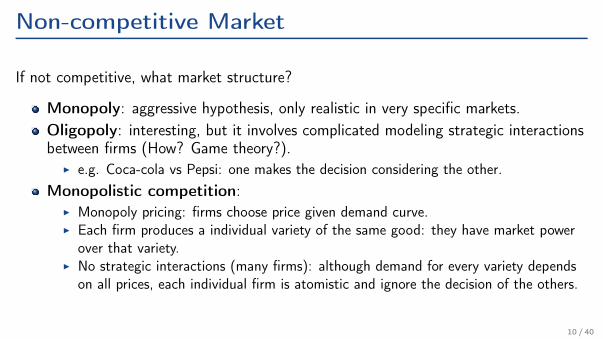
Non-competitive Market

If not competitive, what market structure?

Monopoly: aggressive hypothesis, only realistic in very specific markets.Oligopoly: interesting, but it involves complicated modeling strategic interactionsbetween firms (How? Game theory?).

I e.g. Coca-cola vs Pepsi: one makes the decision considering the other.Monopolistic competition:

I Monopoly pricing: firms choose price given demand curve.I Each firm produces a individual variety of the same good: they have market power

over that variety.I No strategic interactions (many firms): although demand for every variety depends

on all prices, each individual firm is atomistic and ignore the decision of the others.

10 / 40

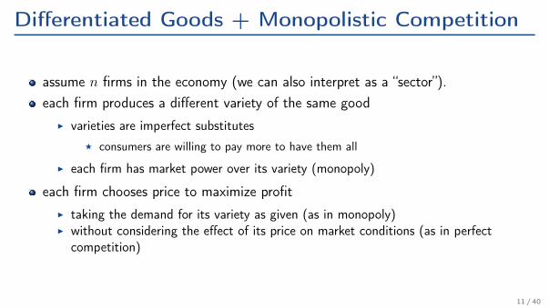
Differentiated Goods + Monopolistic Competition

assume n firms in the economy (we can also interpret as a “sector”).each firm produces a different variety of the same good

I varieties are imperfect substitutesF consumers are willing to pay more to have them all

I each firm has market power over its variety (monopoly)

each firm chooses price to maximize profitI taking the demand for its variety as given (as in monopoly)I without considering the effect of its price on market conditions (as in perfect

competition)

11 / 40

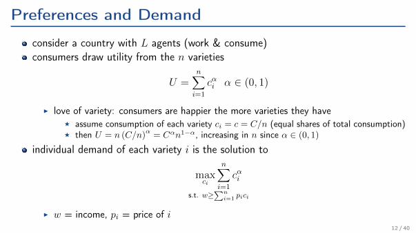
Preferences and Demand

consider a country with L agents (work & consume)consumers draw utility from the n varieties

U =n∑i=1

cαi α ∈ (0, 1)

I love of variety: consumers are happier the more varieties they haveF assume consumption of each variety ci = c = C/n (equal shares of total consumption)F then U = n (C/n)

α= Cαn1−α, increasing in n since α ∈ (0, 1)

individual demand of each variety i is the solution to

maxci

n∑i=1

cαi

s.t. w≥∑n

i=1pici

I w = income, pi = price of i12 / 40

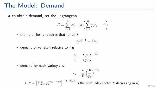
The Model: Demand

to obtain demand, set the Lagrangean

L =n∑i=1

cαi − λ(

n∑i=1

pici − w)

I the f.o.c. for ci requires that for all i

αcα−1i = λpi

I demand of variety i relative to j is

cicj

=

Çpipj

å− 11−α

I demand for each variety i is

ci =w

P

ÅP

pi

ã 11−α

F P =î∑n

i=1 p−α/(1−α)i

ó−(1−α)/αis the price index (note: P decreasing in n)

13 / 40

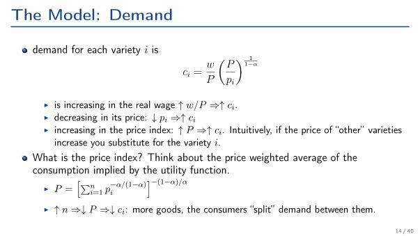
The Model: Demand

demand for each variety i is

ci =w

P

ÇP

pi

å 11−α

I is increasing in the real wage ↑ w/P ⇒↑ ci.I decreasing in its price: ↓ pi ⇒↑ ciI increasing in the price index: ↑ P ⇒↑ ci. Intuitively, if the price of “other” varieties

increase you substitute for the variety i.What is the price index? Think about the price weighted average of theconsumption implied by the utility function.

I P =[∑n

i=1 p−α/(1−α)i

]−(1−α)/αI ↑ n⇒↓ P ⇒↓ ci: more goods, the consumers “split” demand between them.

14 / 40

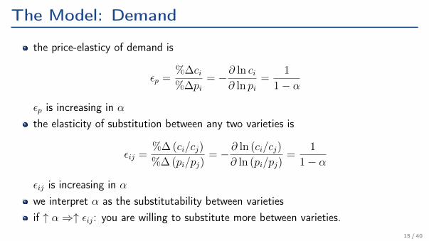
The Model: Demand

the price-elasticy of demand is

εp =%∆ci%∆pi

= −∂ ln ci∂ ln pi

=1

1− α

εp is increasing in αthe elasticity of substitution between any two varieties is

εij =%∆ (ci/cj)

%∆ (pi/pj)= − ∂ ln (ci/cj)

∂ ln (pi/pj)=

1

1− α

εij is increasing in αwe interpret α as the substitutability between varietiesif ↑ α⇒↑ εij: you are willing to substitute more between varieties.

15 / 40

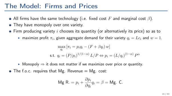
The Model: Firms and Prices

All firms have the same technology (i.e. fixed cost F and marginal cost β).They have monopoly over one variety.Firm producing variety i chooses its quantity (or alternatively its price) so as to

I maximize profit πi, given aggregate demand for their variety qi = Lci and w = 1.

maxqi

[πi = piqi − (F + βqi)w]

s.t. qi = (P/pi)1/(1−α) L/P ⇔ pi = (L/qi)

(1−α) Pα

I Monopoly ⇒ it does not matter if we maximize over price or quantity.

The f.o.c. requires that Mg. Revenue = Mg. cost:

Mg R. = pi +∂pi∂qi

qi = β = Mg. C.

16 / 40

Monopolistic Competition

qi

MC

MR

q∗i

Cost, Price MC = β and MR = pi + ∂pi∂qiqi.

Perfect competition: MR = p!Perfect competition: MR is flat!

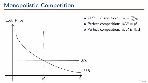
17 / 40

Monopolistic Competition

qi

MC

MR

AC

q∗i

Cost, Price

p

AC∗

p∗i

ProfitMC = β and MR = pi + ∂pi

∂qiqi.

Average cost = AC = F/q + β.Since, ∂pi

∂qi< 0,

MR(q) < p(q).Profit: π = p× q − AC(q)× q

18 / 40

The Model: Firms and Prices

differentiate pi with respect to qi and using the aggregate demand to obtain

pi +∂pi∂qi

qi = pi − (1− α)

ÇL

qi

å(1−α)Pα

︸ ︷︷ ︸=pi

= β

⇒ pi − (1− α)pi = β

hence

pi =β

αand qi =

ÇPα

β

å1/(1−α) L

P

19 / 40

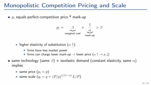
Monopolistic Competition Pricing and Scale

pi equals perfect-competition price * mark-up

pi = β︸︷︷︸marginal cost

× 1

α︸︷︷︸mark-up

> β

I higher elasticity of substitution (α ↑):F firms have less market powerF firms can charge lower mark-up → lower price (α ↑ → p ↓)

same technology (same β) + isoelastic demand (constant elasticity, same α)implies

I same price (pi = p)I same scale (qi = q = (P/p)1/(1−α) L/P )

20 / 40

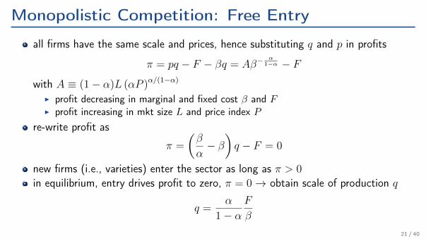
Monopolistic Competition: Free Entry

all firms have the same scale and prices, hence substituting q and p in profits

π = pq − F − βq = Aβ−α

1−α − F

with A ≡ (1− α)L (αP )α/(1−α)

I profit decreasing in marginal and fixed cost β and FI profit increasing in mkt size L and price index P

re-write profit as

π =

Çβ

α− βåq − F = 0

new firms (i.e., varieties) enter the sector as long as π > 0

in equilibrium, entry drives profit to zero, π = 0→ obtain scale of production q

q =α

1− αF

β

21 / 40

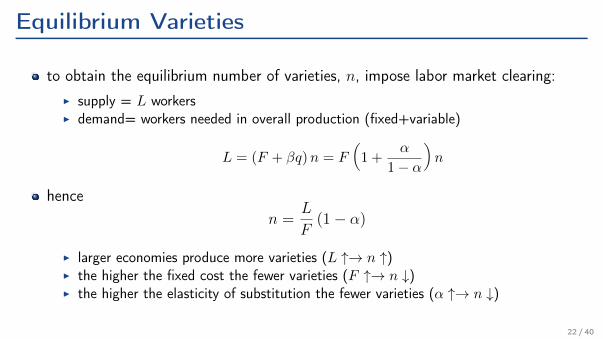
Equilibrium Varieties

to obtain the equilibrium number of varieties, n, impose labor market clearing:I supply = L workersI demand= workers needed in overall production (fixed+variable)

L = (F + βq)n = F

Å1 +

α

1− α

ãn

hencen =

L

F(1− α)

I larger economies produce more varieties (L ↑→ n ↑)I the higher the fixed cost the fewer varieties (F ↑→ n ↓)I the higher the elasticity of substitution the fewer varieties (α ↑→ n ↓)

22 / 40

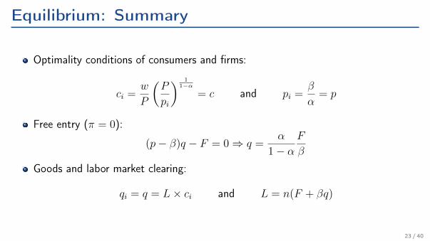
Equilibrium: Summary

Optimality conditions of consumers and firms:

ci =w

P

ÇP

pi

å 11−α

= c and pi =β

α= p

Free entry (π = 0):

(p− β)q − F = 0⇒ q =α

1− αF

β

Goods and labor market clearing:

qi = q = L× ci and L = n(F + βq)

23 / 40

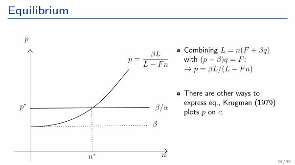
Equilibrium

n

β/α

n∗

p∗

p =βL

L− Fn

p

β

Combining L = n(F + βq)with (p− β)q = F :→ p = βL/(L− Fn)

There are other ways toexpress eq., Krugman (1979)plots p on c.

24 / 40

Outline

1. Increasing Returns and Monopolistic Competition

2. Open Economy

3. Pro-Competitive GFT

4. Empirical Evidence

25 / 40

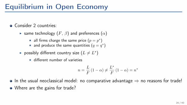
Equilibrium in Open Economy

Consider 2 countries:I same technology (F , β) and preferences (α)

F all firms charge the same price (p = p∗)F and produce the same quantities (q = q∗)

I possibly different country size (L 6= L∗)F different number of varieties

n =L

F(1− α) 6= L∗

F(1− α) = n∗

In the usual neoclassical model: no comparative advantage ⇒ no reasons for trade!Where are the gains for trade?

26 / 40

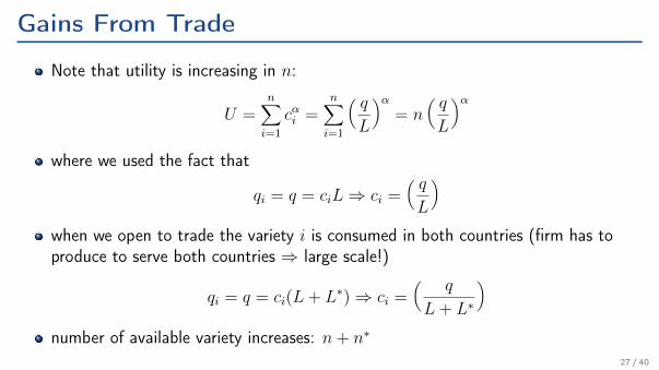
Gains From Trade

Note that utility is increasing in n:

U =n∑i=1

cαi =n∑i=1

Å qL

ãα= n

Å qL

ãαwhere we used the fact that

qi = q = ciL⇒ ci =Å qL

ãwhen we open to trade the variety i is consumed in both countries (firm has toproduce to serve both countries ⇒ large scale!)

qi = q = ci(L+ L∗)⇒ ci =Å q

L+ L∗

ãnumber of available variety increases: n+ n∗

27 / 40

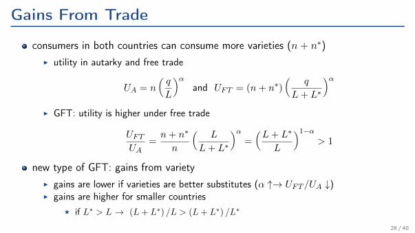
Gains From Trade

consumers in both countries can consume more varieties (n+ n∗)I utility in autarky and free trade

UA = n

Åq

L

ãαand UFT = (n+ n∗)

Åq

L+ L∗

ãαI GFT: utility is higher under free trade

UFTUA

=n+ n∗

n

ÅL

L+ L∗

ãα=

ÅL+ L∗

L

ã1−α> 1

new type of GFT: gains from varietyI gains are lower if varieties are better substitutes (α ↑→ UFT /UA ↓)I gains are higher for smaller countries

F if L∗ > L → (L+ L∗) /L > (L+ L∗) /L∗

28 / 40

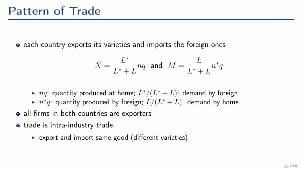
Pattern of Trade

each country exports its varieties and imports the foreign ones

X =L∗

L∗ + Lnq and M =

L

L∗ + Ln∗q

I nq: quantity produced at home; L∗/(L∗ + L): demand by foreign.I n∗q: quantity produced by foreign; L/(L∗ + L): demand by home.

all firms in both countries are exporterstrade is intra-industry trade

I export and import same good (different varieties)

29 / 40

Outline

1. Increasing Returns and Monopolistic Competition

2. Open Economy

3. Pro-Competitive GFT

4. Empirical Evidence

30 / 40

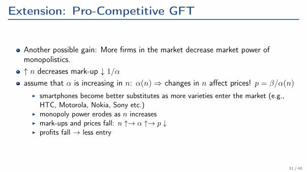
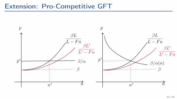
Extension: Pro-Competitive GFT

Another possible gain: More firms in the market decrease market power ofmonopolistics.↑ n decreases mark-up ↓ 1/α

assume that α is increasing in n: α(n)⇒ changes in n affect prices! p = β/α(n)

I smartphones become better substitutes as more varieties enter the market (e.g.,HTC, Motorola, Nokia, Sony etc.)

I monopoly power erodes as n increasesI mark-ups and prices fall: n ↑→ α ↑→ p ↓I profits fall → less entry

31 / 40

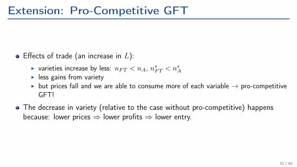
Extension: Pro-Competitive GFT

Effects of trade (an increase in L):I varieties increase by less: nFT < nA, n∗FT < n∗AI less gains from varietyI but prices fall and we are able to consume more of each variable → pro-competitive

GFT!

The decrease in variety (relative to the case without pro-competitive) happensbecause: lower prices ⇒ lower profits ⇒ lower entry.

32 / 40

Extension: Pro-Competitive GFT

n

β/α

n∗

p∗

βL

L− Fn

p

β

βL′

L′ − Fn

n

β/α(n)

n∗

p∗

βL

L− Fn

p

β

βL′

L′ − Fn

33 / 40

Outline

1. Increasing Returns and Monopolistic Competition

2. Open Economy

3. Pro-Competitive GFT

4. Empirical Evidence

34 / 40

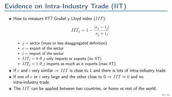
Evidence on Intra-Industry Trade (IIT)

How to measure IIT? Grubel y Lloyd index (IIT ):

IITj = 1− |ej − ij|ej + ij

I j = sector (more or less disaggregated definition)I e = export of the sectorI i = import of the sectorI IITj = 0 if j only imports or exports (no IIT)I IITj = 1 if j imports as much as it exports (max IIT)

If e and i very similar ⇒ IIT is close to 1 and there is lots of intra-industry trade.If one of e or i very large and the other close to 0 ⇒ IIT ≈ 0 and nointra-industry trade.The IIT can be applied between two countries, or home vs rest of the world.

35 / 40

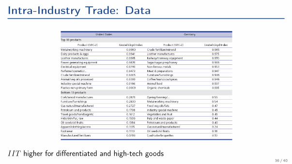
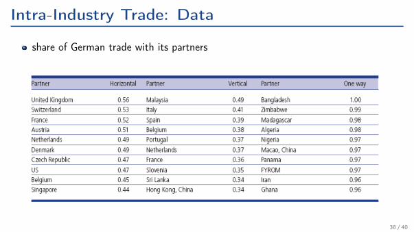
Intra-Industry Trade: Data

IIT higher for differentiated and high-tech goods36 / 40

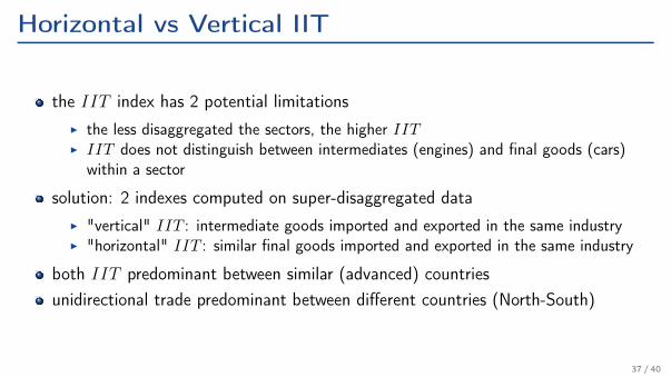
Horizontal vs Vertical IIT

the IIT index has 2 potential limitationsI the less disaggregated the sectors, the higher IITI IIT does not distinguish between intermediates (engines) and final goods (cars)

within a sector

solution: 2 indexes computed on super-disaggregated dataI "vertical" IIT : intermediate goods imported and exported in the same industryI "horizontal" IIT : similar final goods imported and exported in the same industry

both IIT predominant between similar (advanced) countriesunidirectional trade predominant between different countries (North-South)

37 / 40

Intra-Industry Trade: Data

share of German trade with its partners

38 / 40

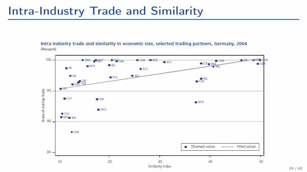
Intra-Industry Trade and Similarity

39 / 40

Summary

IRS + differentiated goods → monopolistic competitionI monopolist’s price is decreasing in substitutability

larger markets → more varietiesmore varieties → happier consumersefect of trade = increase market size

I more varieties → more varieties can be consumed in both countriesI gains from trade = gains from variety

pattern of specialization and tradeI each country specializes in a number of different varieties depending on its sizeI each country exports all domestic and imports all foreign varieties: intra-industry

trade

smaller countries benefit more from trade40 / 40