Embed Size (px)
Citation preview

FEDERAL RESERVE BANK OF SAN FRANCISCO
WORKING PAPER SERIES
The views in this paper are solely the responsibility of the author and should not be interpreted as reflecting the views of the Federal Reserve Bank of San Francisco or the Board of Governors of the Federal Reserve System. This paper was produced under the auspices of the Center for Pacific Basin Studies within the Economic Research Department of the Federal Reserve Bank of San Francisco.
Working Paper 2008-01
http://www.frbsf.org/publications/economics/papers/2008/wp08-01bk.pdf
International Financial Remoteness and
Macroeconomic Volatility
Andrew K. Rose
Haas School of Business
University of California, Berkeley
Mark M. Spiegel
Federal Reserve Bank of San Francisco
November 2007

International Financial Remoteness and Macroeconomic Volatility Andrew K. Rose and Mark M. Spiegel*
Draft Revised as of November 19, 2007
Abstract This paper shows that proximity to major international financial centers seems to reduce business cycle volatility. In particular, we show that countries that are further from major locations of international financial activity systematically experience more volatile growth rates in both output and consumption, even after accounting for domestic financial depth, political institutions, and other controls. Our results are relatively robust in the sense that more financially remote countries are more volatile, though the results are not always statistically significant. The comparative strength of this finding is in contrast to the more ambiguous evidence found in the literature. Keywords: empirical, data, cross-section, business cycle, capital, distance, proximity. JEL Classification Numbers: E32, F32 Andrew K. Rose Mark M. Spiegel (correspondence) Haas School of Business Federal Reserve Bank of San Francisco University of California 101 Market St. Berkeley, CA USA 94720-1900 San Francisco CA 94105 Tel: (510) 642-6609 Tel: (415) 974-3241 Fax: (510) 642-4700 Fax: (415) 974-2168 E-mail: [email protected] E-mail: [email protected] * Rose is B.T. Rocca Jr. Professor of International Trade and Economic Analysis and Policy in the Haas School of Business at the University of California, Berkeley, NBER research associate and CEPR Research Fellow. Spiegel is Vice President, Economic Research, Federal Reserve Bank of San Francisco. Helpful comments were received from Henning Bohn, Galina Hale, Linda Goldberg, Gordon Hanson, Ken Kletzer, Phil Lane, Enrique Mendoza, Romain Ranciere, participants at the IMF and Cornell University Conference on “New Perspectives on Financial Globalization” And two anonymous referees. We thank Menzie Chinn for his capital controls data. Rose thanks the Monetary Authority of Singapore and the National University of Singapore for hospitality during the course of this research. Christopher Candelaria provided excellent research assistance. The views expressed below do not represent those of the Federal Reserve Bank of San Francisco or the Board of Governors of the Federal Reserve System, or their staffs. A current version of this paper, key output, and the main STATA data set used in the paper are available at http://faculty.haas.berkeley.edu/arose.

1
1. Introduction and Motivation
This paper introduces a new stylized fact; countries that are remote from international
financial activity are systematically more volatile. While most of this paper is concerned with
establishing the empirical finding, we begin by motivating our study.
The effect of financial integration on macroeconomic volatility is ambiguous in theory
and uncertain in practice. Theoretically, if integration enhances financial development, it may
reduce the volatility of investment and thereby output. It can do this by easing adjustment,
allowing for greater diversification of risk, or by mitigating shocks to credit supply. But
increased international financial integration can also leave a country more exposed to external
shocks and more specialized in production, both of which can exacerbate output volatility.
Theory is similarly agnostic about the implications of increased international financial
integration for consumption volatility.1 While rational agents would typically not respond to
enhanced consumption-smoothing opportunities by increasing their specialization sufficiently to
generate a net increase in consumption volatility, the greater exposure to international shocks
leaves the net impact on consumption volatility ambiguous in theory.
The empirical evidence on the relationship between financial integration and
macroeconomic volatility (of both output and consumption) is similarly mixed. In the next
section, we provide a brief review of the literature, which reports a spectrum of results ranging
from increased volatility, to decreased volatility, to no response to increased financial
integration. One reason why these studies present weak results may be the difficulty of
measuring international financial integration, at least for a broad set of countries. The literature
has used both de jure and de facto measures. De jure measures have usually been based on the
1 Throughout, we refer to volatility of growth in consumption (output) as consumption (output) volatility for simplicity.

2
International Monetary Fund’s index of capital account restrictions, sometimes adjusted for
intensity by Quinn (1997). De facto measures usually examine ratios of a country’s international
capital flows or stocks to its gross domestic product.
Difficulties exist with both measures. De jure measures are only coarsely corrected for
the magnitude and effectiveness of government restrictions (Edison, et al, 2002). De jure
measures are also likely to suffer from endogeneity issues, as governments might respond to
macroeconomic turbulence by imposing restrictions on capital movements. De facto measures
may also suffer from endogeneity issues, as openness may be a function of shocks that also
affect volatility.
We identify a nation’s “financial remoteness” with its physical distance from world
financial activity, based on the idea that the cost of financial intermediation increases with
distance. Theoretical arguments in the literature supporting this claim, such as the possibility
that information costs of monitoring loans increases with geographic distance, are discussed
below. Given this conjecture, it follows that we expect more remote countries to be less
financially integrated with the rest of the world than those in close proximity to major
international financial centers, holding all else equal.
Our primary measure of international financial remoteness is the natural logarithm of the
great-circle distance to the closest major financial center (London, New York, or Tokyo). We
search for, and find, an effect of this measure of remoteness on volatility.2 To check the
robustness of our results, we verify our results for a number of alternative measures as well.
2 Henning Bohn has pointed out that Hong Kong may be a reasonable alternative to Tokyo. We choose Tokyo instead of Hong Kong because of the much larger size of its market. For example, the 2004 CPIS lists the Japanese market as having over 2 trillion dollars in total portfolio investment, of which 694 million dollars was exposure to the United States. By way of contrast, Hong Kong had 401 million dollars in external portfolio investment, of which 59 million was exposure to the United States. In any event, we re-ran our specifications using Hong Kong as the third major financial center (instead of Tokyo) and obtained very similar results.

3
Our analysis of the relationship between geographic measures of a country’s integration
with the world economy, and their manifestation in macroeconomic volatility can therefore be
interpreted as examination of a joint hypothesis: 1) countries closer to major financial centers are
more financially integrated (holding all else equal), and 2) financial integration reduces
macroeconomic volatility. Because the first component of this joint hypothesis is less standard,
we sketch out the theoretical justifications for this link below. We note that maintaining this first
link delivers a plausibly exogenous measure of integration. Unlike measures of financial
integration used in the literature, distances to major world financial centers are not influenced by
policy, and are invariant to shocks that may affect macroeconomic volatility. To rule out the
possibility that our results are driven by New York, London and Tokyo’s emergence as financial
centers due to the superior performance of neighboring countries, we remove the largest
countries from our sample as a robustness exercise. It seems implausible to us that the
performance of individual smaller countries would have any effect on the location of major
international financial centers.
We find that the relationship between financial remoteness and volatility is robustly
positive and usually statistically significant. In our default specification, a one standard
deviation increase in financial remoteness (roughly equal to that between Algeria and Kiribati)
results in a 15.4 percent increase in output volatility relative to the sample mean. The significant
effect of financial remoteness is reasonably insensitive to a number of checks, including
dropping larger countries.
We do not wish to overstate the strength and resilience of our results. Our results are not
completely insensitive; for instance, dropping rich countries reduces the statistical (though not
the economic) significance of the relationship. While we always find that greater remoteness is

4
associated with more business cycle volatility, our estimates are not always significantly
different from zero. This is in contrast to the effect of institutional quality in our specification,
which is significant throughout with its predicted sign. This makes us cautious in our
interpretation. Still, our results on remoteness are much stronger than the effects on volatility of
other conditioning variables, such as those of domestic credit conditions, openness, or
government size. Moreover, they demonstrate a stronger linkage between financial conditions
and macroeconomic volatility than is typically found in the literature.
2. Literature Review
The analysis in this paper relies on geography to identify plausibly-exogenous differences
in international financial integration – based on differences in access to financial services from
abroad – that can be brought to bear on the question of international financial integration and
macroeconomic volatility. We now ground our empirical work in the literature, using two
strands of recent work: 1) the role of geography in international financial flows, and 2) the
relationship between international financial integration and macroeconomic volatility.
The literature on the role of geography in financial flows begins with a conundrum; the
cost of moving financial assets seems like it should be negligible, but appears to be high in
practice. The cost of sending assets from New York to Singapore is roughly equivalent to that of
sending assets from New York to Los Angeles. However, exercises that link asset flows to
distance usually perform rather well, analogous to “gravity” models of trade. This raises the
question of why there is “home bias” in asset holdings; distance influences international asset
flows in a manner qualitatively similar to flows of goods.

5
One answer supported by empirical evidence is that information asymmetries appear to
increase in distance. Coval and Moskowitz (1999, 2001) demonstrate that fund managers in the
United States tend to invest more heavily in and earn abnormally large returns from investing in
firms in close proximity, particularly from smaller firms where information asymmetries would
be expected to be greater. Malloy (2005) finds that geographically proximate analysts tend to be
more accurate than those that are located farther away, again with the result being most
pronounced among smaller firms. Portes and Rey (2005) introduce a variety of indicators of
information asymmetries into a gravity specification of international asset flows and find that
these indicators are significantly negatively related to equity trade volumes. Petersen and Rajan
(2002) find that borrower quality increases with distance, as banks are unwilling to lend at great
distances to problem borrowers whose loans would require more active monitoring. Berger, et al
(2005), find that larger banks, who are also usually regarded as less intensive in the use of “soft”
information in their lending decisions, lend at greater distances than small banks.3
The second strand of the literature that forms the basis for our analysis concerns the
relationship between financial integration and volatility. As noted above, theory is ambiguous
on the sign of this relationship. On one hand, agents rationally respond to increased risk-sharing
opportunities by raising the specialization of the production bundle [e.g. Kalemli-Ozcan,
Sørensen and Yosha (2003)]. This leaves the output bundle more valuable at the country or
regional level, but also more variable. On the other hand, a number of papers [e.g. Caballero and
Krishnamurthy (2001)] demonstrate that poorly-developed financial sectors can exacerbate
volatility, as there are fewer opportunities for firms to smooth investment shocks. Similarly,
papers that consider the implications of financial liberalizations, such as Martinez, Tornell, and
3 Aviat and Couerdacier (2007) explain gravity international finance models by stressing the complementarity between flows in assets and flows in goods. They demonstrate that after accounting for trade flows, the explanatory power of distance in financial flows is halved, but still not eliminated.

6
Westermann (2003), suggest that credit market imperfections can result in a positive relationship
between financial liberalization and macroeconomic volatility.
The empirical evidence concerning the relationship between financial integration and
macroeconomic volatility is also mixed. O’Donnell (2001) finds a positive relationship between
financial openness and macroeconomic volatility in non-OECD economies, but a negative
relationship among OECD countries. Buch, Doepke, and Pierdzioch (2005) find no consistent
link between openness and output volatility among OECD countries. Prasad, et al (2003) find
that the median percentage standard deviation of less financially integrated countries in their
1960-1999 sample is 33% larger than the median of their more financially integrated sub-
sample.4
The primary channel through which financial integration might reduce macroeconomic
volatility is through its impact on financial depth. Acemoglu and Zilibotti (1997) develop a
model where financial deepening allows for greater risk-spreading and reduces macroeconomic
volatility. Aghion, et al, (2005) also develop a model where financial deepening reduces
macroeconomic volatility, as long-term investments become counter-cyclical with increased
financial deepening. They confirm the prediction for a panel of countries, finding that low levels
of financial development are associated with increased volatility in both investment and growth.
From a welfare point of view, one might be more concerned with consumption volatility.
Under standard parameter values, we might expect a reduction in consumption volatility from
increased financial integration. Although agents might respond to increased financial integration
by producing a more specialized output bundle, and thereby increasing output volatility, they
4 The more financially integrated sub-sample in Prasad, et al (2003) is based on a ranking of de facto financial openness, as well as other indicators of financial integration. The paper reports that the division ends up with 22 countries designated as “more financially integrated “ that roughly corresponds to the Morgan Stanley emerging markets stock index, and 33 countries identified as less financially integrated.

7
would be unlikely to do so to the extent that the dampening effect of improved hedging
opportunities would have on consumption volatility is more than offset [e.g. Mendoza (1994),
Baxter and Crucini (1995) and Sutherland (1996)]. Still, to the extent that financial openness
leaves countries more exposed to external shocks, the impact on consumption volatility could be
reversed. Moreover, Levchenko (2005) demonstrates that the predicted reduction in consumption
volatility associated with international financial integration is smaller when agents have
heterogeneous access to international capital markets than are predicted by the representative
agent models in the literature.
The empirical literature is again mixed. In a recent paper, Bekaert, et al (2006) find that
financial liberalization is associated with reduced consumption growth volatility, particularly for
countries with open capital accounts. Kose, et al, (2005) obtain mixed results concerning the
relationship between financial integration and volatility: While they find a negative relationship
over their full sample, they also find that among the more financially integrated countries,
liberalizations tend to be followed by increased consumption volatility. Huizinga and Zhu
(2006) find that integration with international debt markets enhances consumption smoothing for
non-OECD countries, but not for OECD countries. Kose, at al (2003) find a modest negative
relationship between their measure of de jure financial integration, an index of the severity of
capital account restrictions, and the volatility of private consumption, but fail to find a significant
relationship for their de facto financial integration measure.5
An alternative measure used in the literature is the volatility of the share of consumption
in income, which is considered a measure of the extent of consumption smoothing. Using this
measure, Kose, et al, (2003) find a negative relationship between their de facto proxy for
financial integration and consumption smoothing, but they find that this relationship turns 5 The positive relationship becomes insignificant in their instrumented panel regressions.

8
positive beyond some level of financial development. They conclude that financial integration
does increase consumption smoothing beyond some threshold of financial development.
Similarly, Kose, et al (2007) find that financial integration increases consumption smoothing for
developed economies, but not for developing or emerging market economies. Prasad, et al,
(2003) fail to find any measurable correlation between financial integration and the ratio of
consumption volatility to income volatility.
Finally, we note that the role of geography in macroeconomic volatility has already been
explored in the literature on international asset trade, e.g., Martin and Rey (2004, 2006). In these
models, exchanges of international assets are assumed to carry an additional transaction cost
relative to the exchange of domestic assets. The level of financial integration is then declining in
these transactions costs. When these transactions costs are posited to be increasing in physical
distance, as in Portes and Rey (2005), international financial integration between two countries is
decreasing in their physical distance. Similarly, Rose and Spiegel (2007) introduce a model
where the cost of moving assets to offshore banks is increasing in distance, and find that the
share of offshore banking is decreasing in physical distance from the offshore financial center.6
Our review of the literature leads us to conclude that the theoretical underpinnings of our
project are well-established and intuitive; existing theory motivates our empirical analysis. The
value-added in this paper lies in its empirics.
3. Strategy and Methodology
6 Our reduced-form specification allows geographic proximity to affect macroeconomic volatility through a variety of channels. It can directly affect volatility by enhancing the consumption or output-smoothing opportunities available domestically. Alternatively, access to external financial services has been shown to affect domestic financial conditions [e.g. Rose and Spiegel (2007)]. As such, geographic proximity may also indirectly affect macroeconomic volatility through its impact on the domestic financial sector. Of course, it is difficult empirically to distinguish this impact from differences in domestic financial conditions that are unrelated to geography. We therefore condition on domestic credit conditions before searching for the additional effect of remoteness.

9
The objective of our empirical work is to see if a country’s geographic location
“matters,” and in particular to determine if countries that are further from international financial
activity suffer more business cycle volatility, other things being equal. We do not use a
structural theory linking the two concepts. Further, there are only imperfect measures of a
number of key variables. Accordingly, our strategy is to take a reduced-form approach that
encompasses existing determinants of cyclic volatility, and subject it to intense sensitivity
analysis.7
Our default specification is as follows:
Voliτ=βIntFinRemi + γ1DomFiniτ + γ2Instiτ + γ3Openiτ + γ4Govtiτ + γ0 + εi
where:
• Voliτ is a measure of business cycle volatility for country i over period τ,
• IntFinRemi is a measure of international financial remoteness,
• {γ} are a set of nuisance coefficients,
• DomFin is a measure of domestic financial depth,
• Inst is a measure of domestic political-economy institutions,
• Open is the ratio of trade to GDP,
• Govt is the ratio of government spending to GDP, and
• ε represents other (hopefully unrelated) determinants of business cycle volatility.
The coefficient of interest to us is β, which measures the effect of international financial
remoteness on business cycle volatility. A positive and significant coefficient indicates that
greater international financial remoteness is associated with higher business cycle volatility,
7 An appendix contains a sketch of a theoretical model that can be used to more rigorously justify our intuition.

10
ceteris paribus. We estimate this cross-sectional regression with OLS, using standard errors
robust to the presence of heteroskedasticity.
There are a variety of measures of business cycle volatility, none obviously superior to
any other. Indeed, it is also unclear how to measure our key regressors: international financial
remoteness, domestic financial depth, and institutions. Our strategy is to choose what we think
of as being obvious and reasonable choices and check that our key results are robust to
reasonable alternatives.
We measure business cycle volatility for country i over period τ via the standard
deviation of real GDP growth (the annual first-difference of the natural logarithm of real GDP),
for the eleven year period between 1994 and 2004 inclusive.8 We also examine both longer (27-
) and shorter (5-year) periods, and pool our data across all five 11-year periods between 1950
and 2004. For further sensitivity analysis, we check both the comparable volatility of
consumption and the lowest GDP growth rate during the 11-year period. Finally, we estimate
our cross-sections using volatilities calculated over the entire 55 years of data available, de-
trending real GDP in three different ways (deviations of growth rates from their means, and via
both the Baxter-King and Hodrick-Prescott filters).
Our key regressor is international financial remoteness. As this is the novelty of the
paper, the literature is of little help.9 We begin our analysis with a simple measure that we
consider to be crude but convenient; we use the natural logarithm of the great-circle distance to
the closest major financial center (London, New York, or Tokyo), and drop Japan, the UK and 8 We choose 11-year periods because we have 55 years of annual data between 1950 and 2004 inclusive. This period is long enough to include entire business cycles. For sensitivity analysis, we also examine periodicities that are both shorter and longer. 9 We compare our geographic-based measure of financial remoteness to a variety of more conventional measures of capital mobility in an appendix. Our measure is consistently correlated with other measures. For instance, the popular dummy variable taken from the IMF’s Annual Report on Exchange Arrangements and Exchange Restrictions (where unity indicates controls) is positively correlated with financial remoteness. However, the correlations are all small, indicating non-trivial measurement error in at least some indicators of capital mobility.

11
the US from our estimation. By this measure, Mauritius and Lesotho are the countries most
remote from international financial activity (Belgium and the Netherlands are the least).
International financial remoteness is mapped in Figure 1. We split our sample into thirds on the
basis of remoteness, considering the least financially remote countries to be “proximate,” the
most remote to be “remote” and the middle third the be “average.” It can be seen that Canada,
the Caribbean, Europe, and a few East Asians are characterized as “proximate,” while much of
South America, Southern Africa, South Asia, and the Antipodes are remote.
To check that our results do not depend inordinately on this precise measure, we also use
three other measures of international financial remoteness (and a number of perturbations
thereof). First, we use the distance from a country to the closest offshore financial center.
Second, we measure the distance to countries that have large gross international stocks of
international debt or assets, using the CPIS data set.10 Third, we measure the distance to
countries that have large gross capital exports on a flow basis, using IFS data.11
We include four additional controls to purge business cycle volatility of extraneous
influences before we search for the effects of international financial remoteness.
The importance of domestic financial depth has been stressed by, among others,
Acemoglu and Zilibotti (1997) and Bekaert, et al, (2006). We use domestic credit provided by
the banking sector, measured as a percentage of GDP, as our default measure. However, we also
use M3 (also as a proportion of GDP) as a check.12
10 In practice, we use the top eight debtors; there is a non-trivial gap between these and the remaining countries. Averaging available CPIS data between 1997 and 2005, these were: the USA; the UK; Germany; France; the Netherlands; Italy; Luxembourg; and Japan, all of whom had at least $50 billion in average liabilities. 11 In practice, we use the top ten capital exporters which seem reasonable and account for most gross capital outflows. For 1994-2004, these were: the UK; the USA; Germany; France; Luxembourg; Ireland; the Netherlands; Japan; Spain; and Belgium. 12 In unreported work we have also extensively examined quasi-money as a proportion of GDP.

12
Acemoglu, Johnson, Robinson, and Thaicharoen (2003) have shown how critical
political-economy institutions are in understanding volatility. For institutions, we use the
popular “polity” measure from the University of Maryland’s Center for International
Development and Conflict Management; it ranges from -10 (strong autocracy) to +10 (strong
democracy). As a check, we also use a measure of executive constraints (“xconst” from the
same source), which ranges from 1 (unlimited authority) to 7 (executive parity or
subordination).13
We also condition for trade openness, which has been shown to have a positive effect on
macroeconomic volatility in some studies [e.g. Karras and Song (1996), Kose, et al, (2003)], but
has been shown to have no measurable impact on volatility in others [Razin and Rose (1994)].14
Finally, we condition on government expenditure as a share of GDP, which was shown by
Bekaert, et al (2006) to exacerbate consumption volatility
Figure 2 contains a cross-country scatter-plot of the raw data; business cycle – the
dependent variable in our regression analysis – is plotted on the y-axis against international
financial remoteness on the x-axis. Figure 3 is a comparable plot once the effects of the four
nuisance variables have been taken out through linear regressions. Both show evidence of a
positive relationship between business cycle volatility and international financial remoteness.
4. Default Specification Results
13 Acemoglu, et al (2003) demonstrate that the importance of institutions, as measured by the polity variable increase when instrumental variables are used to account for endogeneity. To examine the robustness of our results, we dropped our conditioning variables and re-ran our specification with only the polity variable included. Both checks left the results for our variable of interest intact. This is unsurprising because the correlation between our primary measure of financial remoteness and our polity variable was only -0.35 with a standard error of 0.08. We have added dummy variables for common law, civil law, and different variants of civil law in our regressions, to measure differences in legal institutions. Our results were also robust to the inclusion of such extra controls. 14 Kraay and Ventura (2001) find a negative relationship between trade remoteness, measured as total distance weighted by bilateral trade volumes, and volatility.

13
The results for our benchmark specification are in the first row of Table 1. Distance to
major financial centers enters positively and significantly; financial remoteness is associated
with increased output volatility. Moreover, the effect is economically important. Our coefficient
point estimate indicates that a one standard deviation increase in financial remoteness would
result in about a 15% increase in output volatility relative to the sample mean.
Among our other conditioning variables, the Polity2 variable enters strongly with a
statistically significant effect. It is also economically large; a one standard deviation decrease in
democracy (roughly a six point move for this sample), leads to over a 17% decrease in output
volatility relative to the sample mean.15 The share of GDP spent by the government also enters
at the 5% confidence level. The other conditioning variables are insignificant.16
Our default specification only explains a modest amount of variation in the data, as our
R-squared estimate is approximately 0.22. We do not see this as particularly troubling, given
that our specification is parsimonious and includes a heterogeneous cross-section of countries.17
Overall, our default specification suggests an economically and statistically significant
positive relationship between financial remoteness and output volatility. Local institutions, as
measured by our polity variable, appear to have a larger effect, but our variable appears to be at
least as significant as domestic financial sector depth.18,19
15 When we use the log of settler mortality as an IV for polity, as advocated by Acemoglu et al (2003), the coefficient of interest to us falls from 1.00 (robust standard error of .38) to .85 (1.03). The loss of precision is associated with a loss of over half our observations, from 143 down to 63. 16 Dropping all the controls, or leaving just the polity control leaves our result intact. 17 R-squared estimates were suppressed, but are all around this value and are available from the authors upon request. 18 We have also added the mean level of real GDP per capita and its square to the list of regressors in our default regression. In this case, our key coefficient on remoteness falls from 1.00 (se .38) to .61 (.34). The latter two terms are significantly different from zero at the .06 level. We thank Ken Kletzer for this suggestion. 19 When we add Chinn and Ito’s measure of capital mobility to our default regression, it enters the regression negatively, but insignificantly. Its presence reduces the key coefficient from 1.00 (robust standard error of .38) to .87 (.38) at the cost of two observations.

14
5. Robustness Checks
We now check that our results are reasonably insensitive to some of the many
assumptions that underlie our default results. Our first checks are in the remainder of Table 1.
First, we alter the period of time (τ) over which the variables are calculated. The default
period is the final (1994-2004) 11-year period; but β stays positive and significant if either longer
(27- ) or shorter (5-year) periods are used, or if we use data pooled over all five 11-year
periods.20
Our positive and significant effect of remoteness on volatility remains if we drop either
countries with greater than 25 million people, or those with more than ten million. This is
important for our maintained exogeneity assumption, as smaller countries are unlikely to have
influenced which nation would emerge as the major world financial centers.
Our results are weakened statistically (though not economically) when we exclude richer
countries (measured either as those with real GDP per capita of more than $20,000 or
$10,000).21,22 This makes us cautious in our claims. However, our results are insensitive to a
number of other perturbations to the framework. For instance, removing outliers – defined as
countries with residuals that lie more than two standard deviations from zero – only increases our
key coefficient. We have added both average country population and country real GDP per
capita, and our key coefficient remains statistically positive. Adding regional dummies
(computed using standard World Bank groupings) also has little effect, as does dropping
20 While it is reassuring to us that the pooled coefficient is significantly positive, it turns out that there is considerable time-variation in the coefficient. We return to this issue below when we discuss Table 5. 21 We have formally tested the hypothesis that the (37) high-income countries in our sample (as determined by the World Bank) have a slope coefficient for financial remoteness that is different from the coefficient of the entire sample. High-income countries have a higher slope, but only by an amount that is economically small (.17) and insignificantly different from zero at the .05 level. 22 When we weigh our observations by the natural logarithm of real GDP, the coefficient on financial remoteness falls slightly (to .93) but retains its statistical significance (with a t-ratio of over 11). When we remove the bottom half of the sample measured in terms of total real GDP, the coefficient on financial remoteness falls from 1.00 (standard error of .38) for the full sample, to .46 (.30) on the largest half of the sample.

15
countries from various regions (the exception being dropping the Sub-Saharan Africans, which
results in a positive but statistically insignificant effect).23
We have also both added and changed our default measures of our control variables.
Adding either the natural logarithm of a country’s latitude or dummy variables for island and
landlocked countries also has little effect on our key result. When we use M3 as a percentage of
GDP instead of domestic banking credit, our key coefficient drops some in economic size and
becomes statistically marginal (though the effect of M3 itself is small); the same is true but to a
lesser extent when we measure institutions with constraint on the executive instead of polity.24
Finally, we have used different ways to measure business cycle volatility. When we
follow Acemoglu, Johnson, Robinson, and Thaicharoen (2003) in using the maximal drop of
GDP by substituting the minimal growth rate of GDP (between 1994 and 2004) in place of the
standard deviation of growth, our coefficient becomes negative and significantly so. This is
consistent with our results; if remoteness raises volatility, it should also make the worst year
worse.25
23 While exclusion of the Sub-Saharan African observations resulted in financial remoteness becoming insignificant, our results are robust to the inclusion of a Sub-Saharan African dummy. This implies that variation across Sub-Saharan African nations, rather than the treatment of the region as a group, is important to our regressions. However, the lack of robustness to the exclusion of this group may simply be attributable to the fact that this region represents the largest number of individual observations in our sample, so that dropping the region substantially our sample size and increases our standard error estimates. 24 We have added a number of additional conditioning variables one at a time to our default specification as additional robustness tests. These include: country size, which has been shown to reduce volatility [Head (1995), Crucini (1997)], the standard deviation of government spending, the share of commodity and manufacturing exports, and the intensity of military conflicts. Their inclusion does not affect our qualitative results, in the sense that financial remoteness continues to enter positively and significantly with these extra variables included. The size of remittances on external earnings also enters our default equation insignificantly; we thank Philip Lane for this suggestion. 25 We have added a number of other controls in an appendix to the paper. These include: trade remoteness; dummy variables for a number of prominent languages; inflation; export concentration (in manufacturing); fixed exchange rate regimes; dummy variables for major religions; the currency composition of long-term debt; the proportions of debt that are multilateral, concessional, and short-term; and the number of regional trade agreements that a country belongs to. Their inclusion does not alter our key conclusions; the effect of financial remoteness remains consistently positive on volatility, and it is usually statistically significant.

16
We do not wish to overstate the strength and resilience of our results. While we always
find that greater remoteness is associated with more business cycle volatility, our estimates are
not always significantly different from zero. This is in contrast to the effect of institutions on
volatility, which remains negative and significant throughout our specifications. However, our
results are consistently signed, and similar in magnitude across specifications. Their statistical
significance is also stronger than the effects on volatility of domestic financial depth, openness,
and government spending. The latter three variables have inconsistent and weak effects that are
rarely economically or statistically significant.
6. Sensitivity Analysis
In this section, we show that reasonable variations to our methodology do not destroy our
key finding, namely that remoteness raises volatility.
Our focus in this paper is the effect of international financial remoteness on business
cycle volatility. Since the distance to the closest major financial centers is an imperfect measure
of this remoteness, it is important to check the sensitivity of our results with respect to this key
variable. Table 2 substitutes three different measures of financial remoteness into our default
framework, replacing distance to the closest of the three large international financial centers
(London, New York, and Tokyo). First, we use the (natural logarithm of great-circle) distance to
the closest offshore financial center (OFC), using the forty OFCs tabulated in Rose and Spiegel
(2007). Second, we use the distance to the (eight) countries with the largest gross stocks of
foreign portfolio liabilities, measured using the CPIS data set. Alternatively, we also use the
distance to the (ten) countries with the largest gross stocks of foreign portfolio assets, again using

17
the CPIS data set.26 These are stock measures that indicate the willingness of a country to issue
to, or receive credit from foreigners. We also use the corresponding flow measures, using data
from IFS. In particular, our third measure is distance to the (ten) countries with the largest
capital outflows; as a check, we also use the distance to the countries with the largest capital
inflows. We measure capital flows in two ways, summing flows of “direct” and “portfolio”
either with or without “other” capital flows.27
While we think of the distance to the closest countries as being most relevant, we also
examine average distance to countries with large international financial activity in the middle
panel of Table 2. Finally, in the bottom panel of Table 2, we use distance to the three major
financial centers, but now weigh each of the three distances by the fraction of actual bilateral
transactions between the country and the “big three.” We use the CPIS data set to derive two
sets of weights; the assets that both are sourced from the relevant country (and hosted in
Japan/UK/USA), and those that are hosted in the relevant country (from Japan/UK/USA).28
The results for Table 2 are similar to our benchmark results, though somewhat weaker.
In particular, these different measures of financial remoteness all show a positive relationship of
distance on volatility. The effect of distance to the closest country varies between .5 and .9 in
size, and is typically significantly different from zero; six of the seven coefficients are different
from zero at the .05 level. The average distance to big international financial players also has a
positive effect, but it is never significantly different from zero at conventional levels. Both of the
26 We choose eight and ten respectively since there seem to be obvious breaks in the series, but the exact number of “large” creditors/debtors chosen makes little difference. 27 The latter represent mostly transactions in currency and deposits, loans and trade credits. 28 We average the CPIS data over the 2001-04 surveys inclusively.

18
weighted results are also positive, and the coefficient with host weights is statistically significant.
Overall, we find reassuring the robustness of the results.29
Table 3 is the analogue to Table 1, but uses the volatility of real consumption instead of
real GDP. As discussed above, producers may respond to enhanced international risk-sharing
opportunities by increasing the specialization of output, thereby increasing output volatility.
However, integration also enhances the ability of consumers to hedge this increased risk;
consumption volatility, which is likely to be directly relevant to welfare, may actually decrease
with integration. In fact, we obtain a coefficient for consumption volatility under our default
specification which is close to that for output volatility, though it is only statistically significant
at the 5% confidence level. The sensitivity analysis in the remainder of the table indicates that
this result, like that for output, is reasonably robust. For instance, our results are robust to
entertaining alternate time periods. We also still obtain statistically significant results when
countries over 25 million in population are omitted from our sample (albeit only at the 5% level),
though we no longer obtain significant results when all countries over 10 million population are
dropped. As before, we no longer obtain statistically significant coefficient estimates on our
29 We experiment further with non-geographic concepts of “distance” in Appendix Table II, with limited success. We use three alternative measures of distance: linguistic, legal and cultural. For linguistic distance, we add a dummy variable which is unity if the country shares a language with the UK, US, or Japan (and is zero otherwise). For legal distance, we construct a comparable dummy which is unity if a country shares the common law of the UK and US, or the German civil law of Japan. For cultural distance, we take advantage of data extracted from the World Values survey (http://www.worldvaluessurvey.org/). We focus on the “Traditional/Secular-rational values” which “reflects the contrast between societies in which religion is very important and those in which it is not.” Societies near the traditional pole emphasize the importance of parent-child ties and deference to authority, along with absolute standards and traditional family values, and reject divorce, abortion, euthanasia, and suicide. These societies have high levels of national pride, and a nationalistic outlook. Societies with secular-rational values have the opposite preferences on all of these topics. The data is from Table A-1 (p27) of the internet appendix to "Modernization, Cultural Change, and Democracy: The Human Development Sequence" by Inglehart, Ronald & Christian Welzel, 2005; they represent factors extracted from a much larger underlying data set. Unfortunately though, they are available for only 54 countries. We have had some success with a second dimension of cross-cultural variation, namely that linked with the transition from industrial society to post-industrial societies-which brings a polarization between Survival and Self-expression values (though this seems less cultural than economic to us). This topic might be worthy of further investigation.

19
variable of interest when we eliminate wealthy countries from the sample. The results for
including regional dummies or dropping regions from our sample are also similar.30,31
In summary, while theory may more strongly indicate a positive relationship between
financial remoteness and consumption volatility than output volatility, our results are broadly
similar for both. Since there is some sensitivity to exact model specification, we find reassuring
the insensitivity to the precise concept of macroeconomic volatility.
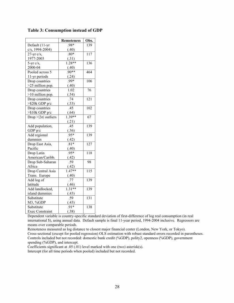
Table 4 uses the entire sample of up to 55 years of (annual) data, instead of focusing on
the last period of time. While examining the standard deviation of growth rates is a reasonable
measure of business cycle volatility over an eleven-year period, de-trending over a longer period
of time is more controversial. Thus we detrend real GDP in two additional ways, using both the
popular Baxter-King and Hodrick-Prescott filters to extract underlying trends.32 We then
compute the standard deviation of detrended real GDP over the entire sample period, and use this
as our dependent variable. We also perform three additional sets of sensitivity checks. First, we
restrict our attention to countries with less than ten million people. Second, we use consumption
in place of GDP. Third, we look at the minimal detrended growth rate instead of the standard
deviation of the growth rate.
Our results are consistently correctly signed, though only five of the twelve coefficients
are significantly different from zero at conventional levels. While we find this reassuring, it is 30 We have also examined alternative measures of the degree of consumption smoothing. For instance, we examined the ratio of consumption growth volatility to income growth volatility as a measure of the intensity of consumption smoothing, as in Kose, et al, (2003) and Prasad, et al, (2003). Also, we examined the correlation between consumption and output, as in Kose, et al (2007). In line with these studies, we found no significant impact of geographic remoteness on these measures. 31 In Figure 4, we provide some relevant graphic evidence. The figure is an unconditional scatter-plot of a standard measure of risk-sharing against our measure of international financial remoteness (distance to the closest major financial center). As the measure of risk-sharing, we use the volatility of consumption growth relative to that of output growth, computed on a country-by-country basis. The calculations are done over our default 11-year period, 1994-2004. The graphic shows a small unconditional positive correlation. 32 We use conventional parameter choices for both filters. For the BK filter, we use a minimum oscillation time of two years, and a maximum of eight, excluding three years at either end of our sample. For the HP filter, we use a smoothing weight of 6 for our annual data.

20
cause for caution. Still, we do obtain statistically significant positive coefficient estimates for a
majority of our specifications using various measures of the standard deviation of consumption
growth.
Our final set of results is in Table 5. In this table we report our benchmark equation
estimated as cross-sections over different periods of time. The results for the five different
eleven-year periods are in the top panel. It is interesting to note that the effect of financial
remoteness seems to rise over time in both economic and statistical significance.33 This evidence
of the growing importance of financial globalization is mirrored in both the 27-year period cross
sections (reported in the middle panel), and the 5-year periods (reported at the bottom of the
table). The impact of international financial remoteness seems to be rising over time, even as
technological barriers to integration seem to be falling. This topic is worth pursuing further.
7. Conclusion
This paper uses geographic proximity as an indicator of international financial
integration, and searches for its manifestations in macroeconomic volatility. We find that
remoteness from financial activity, as measured by the distance to major international financial
centers, increases macroeconomic volatility. We construct a number of alternative measures of
both financial remoteness and volatility and demonstrate that they all appear to share this
positive correlation. The exact size of this effect varies by specification and is not always
significant at standard confidence levels. Still, the coefficient of interest is always positive, and
is often economically large.
We do not wish to overstate the strength of our results, for a number of reasons. First, the
significance of our key coefficient is sensitive to the exclusion of rich countries. Second, 33 The latter effect might be the result of the increasing sample size, but still implies that pooling the data over time is problematic.

21
remoteness does not matter as consistently or robustly as political institutions. Still, we find
stronger results for our indicator of international financial integration than most previous
empirical studies; the effect of remoteness seems comparable to that of domestic financial
markets, openness, or government size.
While the chief purpose of this paper is to establish a stylized fact rather than to explain
it, we briefly provide two thoughts. One answer may be the timing of our study. As we
demonstrate above, the strength of the relationship between financial remoteness and
macroeconomic volatility appears to increase over time. This is consistent with a growing role
for international financial integration, and is consistent with weaker results for studies that rely
on earlier data periods. Alternatively, our measure of financial remoteness may be a better
measure of international financial integration than others, since it is more plausibly exogenous.
Finally, while we believe that the costs of intermediation increase with distance,
assessing the manner in which increased costs of risk sharing affect volatility requires a more
structural treatment than that which we have offered here. That is, we have only provided
indirect evidence that remoteness affects volatility through its impact on integration. Thus we
take a narrow interpretation of our results. While we provide evidence that geography (in the
form of distance from major financial centers) matters for macroeconomic volatility, our work
does not shed light on the desirability (or lack thereof) of capital flow restrictions.
There is much room for future research. One could incorporate differences in real
interest rates across countries into our measure of international financial remoteness. Interest
rates have the advantage of varying over time, so that a proper panel study might be possible. It
would also be interesting to investigate the causes of the growing importance of financial
remoteness. One possibility may be that the proliferation of non-standard financial instruments

22
and derivatives facilitate consumption smoothing, but require greater monitoring than more
conventional capital flows; this would increase the importance of geographic proximity. We
leave such extensions to future work.

23
References
Acemoglu, Daron, Simon Johnson, James Robinson, and Yunyong Thaicharoen. (2003), “Institutional Causes, Macroeconomic Symptoms: Volatility, Crises and Growth,” Journal of Monetary Economics, 50, 49-123. Acemoglu, Daron and Fabrizio Zilibotti, (1997), “Was Prometheus Unbound by Chance? Risk, Diversification and Growth,” Journal of Political Economy, 105(4), 709-751. Aghion, Philippe, George-Marios Angelatos, Abhijit Banerjee, Kalina Manova, (2005), “Volatility and Growth: Credit Constraints and Productivity-Enhancing Investment,” NBER Working Paper 11349, May. Baxter, Marianne., and Mario Crucini. (1995), “Business Cycles and the Asset Structure of International Trade,” International Economic Review, 36, 821-854. Bekaert, Geert, Campbell R. Harvey, and Christian Lundblad, (2006), “Growth Volatility and Financial Liberalization,” Journal of International Money and Finance, 25, 370-403. Berger, Allen N., Nathan H. Miller, Mitchell A. Petersen, Raghuram G. Rajan and Jeremy C. Stein. (2005), “Does Function Follow Organizational Form?: Evidence from the Lending Practices of Large and Small Banks,” Journal of Financial Economics, 76, 237-269. Buch, Claudia M., Joerg Doepke, and Cristian Pierdzioch. (2005), “Financial Openness and Business Cycle Volatility,” Journal of International Money and Finance, 24, 744-765. Chinn, Menzie and Hiro Ito. (2006), “What Matters for Financial Development? Capital controls, Institutions and Interactions,” Journal of Development Economics, 81(1), 163-192. Caballero, Ricardo J., and Arvind Krishnamurthy. (2001), “International and Domestic Collateral Constraints in a Model of Emerging Market Crises,” Journal of Monetary Economics, 48, 513-548. Coval, Joshua D., and Tobias J. Moskowitz. (1999), “Home Bias at Home: Local Equity Preference in domestic Portfolios,” Journal of Finance, 54(6), 2045-2073. Coval, Joshua D., and Tobias J. Moskowitz. (2001), “The Geography of Investment: Informed Trading and Asset Prices,” Journal of Political Economy, 109, 811-841 Crucini, Mario J., (1997), “Country Size and Economic Fluctuations,” Review of International Economics, 5(2). 204-220. Edison, Hali J., Ross Levine, Luca Ricci, and Torsten Sløk. (2002), “International Financial Integration and Economic Growth,” Journal of International Money and Finance, 21, 749-776.

24
Head, Allen C., (1995), “Country Size, Aggregate Fluctuations, and International Risk Sharing,” Canadian Journal of Economics, 28(4b), 1096-1119. Huizinga, Harry and Dantao Zhu, (2006), “Domestic and International Finance: How do they Affect Consumption Smoothing?,” mimeo, Tilburg University. Kalemli-Ozcan, Sebnem, Bent E. Sørensen and Oved Yosha, (2003), “Risk Sharing and Industrial Specialization: Regional and International Evidence,” American Economic Review, 93(3), 903-918. Karras, G. and F. Song. (1996), “Sources of Business Cycle Volatility: An Exploratory Study on a Sample of OECD Countries,” Journal of Macroeconomics, 18(4), 621-637. Kose, M. Ayhan, Eswar S. Prasad, and Marco Terrones. (2003), “Financial Integration and Macroeconomic Volatility,” International Monetary Fund Staff Papers, 50, Special Issue, 119-142. Kose, M. Ayhan, Eswar S. Prasad, and Marco Terrones. (2005), “Growth and Volatility in an Era of Globalization,” International Monetary Fund Staff Papers, 52, Special Issue, 31-63. Kose, M. Ayhan, Eswar S. Prasad, and Marco Terrones. (2007), “How Does Financial Globalization Affect Risk Sharing? Patterns and Channels,” mimeo, prepared for Inernational Monetary Fund Conference on New Perspectives on Financial Globalization, Washington DC. Kraay, Aart, and Jaume Ventura. (2001), “Comparative Advantage and the Cross-Section of Business Cycles,” NBER Working Paper 8104, January. Levchenko, Andrei A., (2005), “Financial Liberalization and Consumption Volatility in Developing Countries,” International Monetary Fund Staff Papers, 52(2), 237-259. Malloy, Christopher J., (2005), “The Geography of Equity Analysis,” Journal of Finance, 54(6), 2045-2073. Martin, Philippe, and Hélène Rey, (2004), “Financial Super-markets: Size Matters for Asset Trade,” Journal of International Economics, 64, 335-361. Martin, Philippe, and Hélène Rey, (2006), “Globalization and Emerging Markets: With or Without Crash?,” Martinez, Lorenza, Aaron Tornell, and Frank Westermann, (2003), “Liberalization, Growth, and Financial Crises: Lessons from Mexico and the Developing World,” Brookings Papers on Economic Activity, 2, 1-112. Mendoza, Enrique G., “The Robustness of Macroeconomic Indicators of Capital Mobility,” in L. Leiderman and A. Razin, eds., Capital Mobility: The Impact on Consumption, Investment and Growth, Cambridge University Press, 83-111.

25
Petersen, Mitchell A. and Raghuram G. Rajan, (2002), “Does Distance Still Matter? The Information Revolution in Small Business Lending,” Journal of Finance, 57(6), 2533-2570. Prasad, Eswar S., Kenneth Rogoff, Shang-Jin Wei, and M. Ayhan Kose. (2003), “Effects of Financial Globalization on Developing Countries: Some Empirical Evidence,” International Monetary Fund Occasional Paper no. 220, International Monetary Fund, Washington, DC. Portes, Richard and Hélène Rey. (2005), “The Determinants of Cross-Border Equity Flows,” Journal of International Economics, 65, 269-296. Quinn, Dennis. (1997), “The Correlates of Change in International Financial Regulation,” American Political Science Review, 91(3), September, 531-551. Razin, Assaf and Andrew K. Rose. (1994), “Business Cycle Volatility and Openness: an Exploratory Cross-Sectional Analysis,” in Capital Mobility: The Impact on Consumption, Investment, and Growth,” Leonardo Leiderman and Assaf Razin eds., (Cambridge: Cambridge University Press), 48-76. Rose, Andrew K., and Mark M. Spiegel. (2007), “Offshore Financial Centres: Parasites or Symbionts?,” forthcoming, Economic Journal. Sutherland, Alan. (1996), “Financial Market Integration and Macroeconomic Volatility,” Scandinavian Journal of Economics, 98, 521-539.

26
Table 1: International Financial Remoteness and Business Cycle Volatility Remoteness Bank Credit
%GDP Polity2 Trade
%GDP Govt Exp %GDP
Obs.
Default (11-yr c/s, 1994-2004)
1.00** (.38)
.01 (.01)
-.12** (.04)
.007 (.005)
.05* (.02)
143
27-yr c/s, 1977-2003
.62* (.29)
.00 (.01)
-.16** (.03)
.003 (.003)
.044* (.018)
121
5-yr c/s, 2000-04
1.22** (.35)
-.01 (.01)
-.056 (.044)
.014 (.007)
-.007 (.025)
140
Pooled across 5 11-yr periods
.70** (.20)
.00 (.01)
-.12** (.02)
.009* (.004)
.038** (.011)
475
Drop countries >25 million pop.
1.14** (.39)
.01 (.01)
-.16** (.05)
.002 (.005)
.05 (.03)
106
Drop countries >10 million pop.
1.06* (.50)
.01 (.01)
-.16* (.05)
.002 (.005)
.06 (.03)
79
Drop countries >$20k GDP p/c
.93 (.48)
.01 (.01)
-.12** (.04)
.009 (.007)
.04 (.02)
121
Drop countries >$10k GDP p/c
.62 (.63)
.01 (.01)
-.12* (.05)
.016 (.009)
.03 (.03)
102
Drop >|2σ| outliers .86** (.19)
-.001 (.003)
-.17** (.03)
.006* (.003)
.03* (.01)
77
Add population, GDP p/c
.66* (.33)
.01 (.01)
-.12** (.04)
.009* (.004)
.03 (.02)
143
Add regional dummies
1.31** (.41)
.01 (.01)
-.13** (.04)
.005 (.005)
.017 (.020)
139
Drop East Asia, Pacific
.97* (.40)
.01 (.01)
-.15** (.04)
.008 (.005)
.04 (.02)
127
Drop Latin American/Caribb.
1.08** (.41)
.01 (.01)
-.12** (.04)
.008 (.005)
.05* (.02)
118
Drop Sub-Saharan Africa
.49 (.33)
-.023** (.006)
-.09* (.04)
.010** (.004)
.06 (.03)
98
Drop Central Asia Trans. Europe
1.26** (.39)
.01 (.01)
-.12** (.04)
.006 (.005)
.01 (.02)
115
Add log of latitude
.97* (.41)
.01 (.01)
-.13** (.04)
-.043 (.326)
.007 (.005)
139
Add landlocked, island dummies
1.14** (.43)
.01 (.01)
-.12** (.04)
.009 (.005)
.04 (.02)
139
Substitute M3, %GDP
.69 (.39)
-.00 (.02)
-.11** (.04)
.007 (.006)
.04* (.02)
135
Substitute Exec Constraint
.83* (.35)
.01 (.01)
-.53** (.13)
.007 (.005)
.05* (.02)
141
Substitute Min Growth Rate
-2.2** (.8)
-.01 (.02)
.12 (.09)
-.01 (.01)
-.06 (.05)
143
Dependent variable is country-specific standard deviation of first-difference of log real GDP (in real international $), using annual data. Default sample is final 11-year period, 1994-2004 inclusive. Regressors are means over comparable periods. Remoteness measured as log distance to closest major financial center (London, New York, or Tokyo). Cross-sectional (except for pooled regression) OLS estimation with robust standard errors recorded in parentheses. Coefficients significant at .05 (.01) level marked with one (two) asterisk(s). Intercept (for all time periods when pooled) included but not recorded.

27
Table 2: Different Measures of International Financial Remoteness Distance to Closest: Remoteness Obs. Offshore Financial Center .58
(.30) 146
Eight Largest Gross Debtors (CPIS data set)
.72* (.31)
140
Ten Largest Gross Creditors (CPIS data set)
.71* (.31)
138
Ten Countries with Largest Gross Capital Outflows (IFS data set)
.78* (.32)
134
Ten Countries with Largest Gross Equity + Portfolio Capital Outflows (IFS data set)
.67* (.31)
134
Ten Countries with Largest Gross Capital Inflows (IFS data set)
.50* (.25)
134
Ten Countries with Largest Gross Equity + Portfolio Capital Inflows (IFS data set)
.60* (.30)
134
Average Distance to:
Eight Largest Gross Debtors (CPIS data set) .74 (.50)
140
Ten Largest Gross Creditors (CPIS data set) .65 (.46)
138
Eight Largest Gross Debtors (CPIS data set), Weighted by liabilities
.93 (.60)
140
Ten Largest Gross Creditors (CPIS data set), Weighted by assets
.84 (.61)
138
Ten Countries with Largest Gross Capital Outflows (IFS data set)
.65 (.46)
134
Ten Countries with Largest Gross Capital Inflows (IFS data set)
.50 (.37)
134
Weighted Distance to Major Financial Centers Host Transactions as Weights (CPIS data set)
1.18** (.40)
114
Source Transactions as Weights (CPIS data set)
.57 (.51)
53
Dependent variable is country-specific standard deviation of first-difference of log real GDP (in real international $), using annual data for 11-year period 1994-2004 inclusive. Regressors are comparable means. Cross-sectional OLS estimation with robust standard errors recorded in parentheses. Controls included but not recorded: domestic bank credit (%GDP), polity2, openness (%GDP), government spending (%GDP), and intercept. Coefficients significant at .05 level marked with asterisk. Remoteness measured as log distance. Intercept included but not recorded.
28
Table 3: Consumption instead of GDP Remoteness Obs. Default (11-yr c/s, 1994-2004)
.98* (.40)
139
27-yr c/s, 1977-2003
.80* (.31)
117
5-yr c/s, 2000-04
1.28** (.40)
136
Pooled across 5 11-yr periods
.90** (.24)
464
Drop countries >25 million pop.
.99* (.40)
106
Drop countries >10 million pop.
1.02 (.54)
76
Drop countries >$20k GDP p/c
.74 (.53)
121
Drop countries >$10k GDP p/c
.45 (.64)
102
Drop >|2σ| outliers 1.39** (.21)
67
Add population, GDP p/c
.45 (.36)
139
Add regional dummies
.95* (.42)
139
Drop East Asia, Pacific
.81* (.40)
127
Drop Latin American/Caribb.
.95* (.42)
118
Drop Sub-Saharan Africa
.59 (.42)
98
Drop Central Asia Trans. Europe
1.47** (.40)
115
Add log of latitude
.77 (.46)
139
Add landlocked, island dummies
1.31** (.43)
139
Substitute M3, %GDP
.59 (.43)
131
Substitute Exec Constraint
.91* (.38)
138
Dependent variable is country-specific standard deviation of first-difference of log real consumption (in real international $), using annual data. Default sample is final 11-year period, 1994-2004 inclusive. Regressors are means over comparable periods. Remoteness measured as log distance to closest major financial center (London, New York, or Tokyo). Cross-sectional (except for pooled regression) OLS estimation with robust standard errors recorded in parentheses. Controls included but not recorded: domestic bank credit (%GDP), polity2, openness (%GDP), government spending (%GDP), and intercept. Coefficients significant at .05 (.01) level marked with one (two) asterisk(s). Intercept (for all time periods when pooled) included but not recorded.
29
Table 4: Full-Sample Analysis over 1950-2004 Regressand is Standard Deviation of: Remoteness Obs. 1st- differenced GDP .39
(.23) 66
HP-filtered GDP .37 (.37)
66
BK-filtered GDP .54 (.28)
66
1ST-differenced consumption .68** (.24)
66
HP-filtered consumption .83* (.35)
66
BK-filtered consumption .89* (.37)
66
1st-differcenced GDP, Drop countries with <10 million pop.
.64* (.31)
34
HP-filtered GDP, Drop countries with <10 million pop.
.82** (.31)
34
BK-filtered GDP, Drop countries with <10 million pop.
.50 (.59)
34
Regressand is Minimum of:
1st- differenced GDP Growth -1.13 (.61)
66
HP-filtered GDP -.75 (.96)
66
BK-filtered GDP -1.34 (.79)
66
Dependent variable computed from natural logarithms (in real international $), using annual data over 55-year period 1950-2004 inclusive. Regressors are means over same period. Cross-sectional OLS estimation with robust standard errors recorded in parentheses. Coefficients multiplied by 100; those significant at .05 (.01) level marked with one (two) asterisk(s). Controls included but not recorded: domestic bank credit (%GDP), polity2, openness (%GDP), government spending (%GDP), and intercept. Baxter-King (BK) filter use minimum/maximum oscillation time of 2/8 years, with lead-lag length of 3 years. Hodrick-Prescott (HP) filter uses smoothing weight of 6. Remoteness measured as log distance to closest major financial center (London, New York, or Tokyo).

30
Table 5: Time-Variation in the Effect of International Financial Remoteness 11-year periods Remoteness Obs. 1950-1960 .54
(.31) 40
1961-1971 .24 (.24)
68
1972-1982 .16 (.33)
103
1983-1993 .72* (.28)
121
1994-2004 1.00** (.38)
143
27-year periods
1950-1976 .17 (.28)
54
1977-2003 .62* (.29)
121
5-year periods
1960-1964 .29 (.39)
61
1965-1969 .23 (.24)
76
1970-1974 .47 (.31)
90
1975-1979 .25 (.38)
100
1980-1984 .55 (.36)
107
1985-1989 .61* (.26)
113
1990-1994 .57 (.30)
122
1995-1999 .62 (.32)
142
2000-2004 1.22** (.35)
140
Dependent variable is country-specific standard deviation of first-difference of log real GDP (in real international $), using annual data. Regressors are means over same sample period. Remoteness measured as log distance to closest major financial center (London, New York, or Tokyo). Cross-Sectional OLS estimation with robust standard errors recorded in parentheses. Coefficients significant at .05 (.01) level marked with one (two) asterisk(s). Controls included but not recorded: domestic bank credit (%GDP), polity2, openness (%GDP), government spending (%GDP), and intercept.

31
Figure 1: International Financial Remoteness
International financial remoteness measured as great-circle distance to closest international financial center (New York, London or Tokyo). Countries divided into thirds on the basis of proximity; closest are “proximate,” furthest are “remote,” and middle are “average.” Countries missing from sample or those with an international financial center shaded in white.

32
Figure 2: Simple Scatter-plot of Volatility against Remoteness B
usin
ess
Cyc
le V
olat
ility
Key Variables, 1994-2004International Financial Remoteness
5 6 7 8 9
0
5
10
15
AfghanisAlbania
Netherla
United A
Argentin
Armenia
Antigua
AustraliAustria
Azerbaij
Burundi
Belgium Benin
Burkina Banglade
Bulgaria
Bahrain
BahamasBosnia a
Belarus BelizeBermuda
Bolivia
BrazilBarbadosBrunei
BhutanBotswanaCentral
CanadaSwitzerl
ChileChinaCote d`ICameroon
Congo, R
ColombiaComoros
Cape Ver
Costa RiCuba Cyprus
Czech Re
Djibouti
Dominica
Denmark
DominicaAlgeria
EcuadorEgypt
Eritrea
Spain
Estonia
Ethiopia
Finland
Fiji
France
Micrones
Gabon
Georgia
Germany
Ghana
Guinea
Gambia, Guinea-B
Equatori
Greece
Grenada
Guatemal
Hong KonHonduras
Croatia
Haiti
Hungary
Indonesi
IndiaIreland
Iran
Iraq
IcelandIsrael
ItalyJamaica
Jordan
Kazakhst
Kenya
Kyrgyzst
Cambodia
Kiribati
St. KittKorea, RKuwait
Laos
Lebanon
Liberia
St. Luci
Sri Lank
LesothoLithuani
Luxembou Latvia
Macao
Morocco
Moldova
MadagascMaldives
Mexico
Macedoni
Mali
Malta
Mongolia
Mozambiq
Mauritan Mauritiu
Malawi
MalaysiaNamibia
Niger
Nigeria
Nicaragu
Netherla NorwayNepal
New Zeal
Oman
PakistanPanama
Peru
PhilippiPalau Papua Ne
Poland
Puerto RKorea, D
Portugal Paraguay
Qatar
Romania
Russia
RwandaSaudi Ar
SudanSenegalSingapor
Solomon Sierra L
El Salva
Somalia
Sao Tome
Suriname
Slovak RSloveniaSweden
SwazilanSyria
Chad
TogoThailand
Tajikist
Turkmeni
Tonga
Trinidad
Tunisia
Turkey
Taiwan Tanzania
Uganda
Ukraine
Uruguay
UzbekistSt.Vince
Venezuel
Vietnam
Vanuatu
Samoa
Yemen
Serbia a
South Af
Congo, D
Zambia
Zimbabwe
International financial remoteness measured as great-circle distance to closest international financial center (New York, London or Tokyo)., scattered against standard deviation of output from 1994-2004 inclusive. Figure 3: Scatter-plot of Volatility against Remoteness, Residuals
Bus
ines
s C
ycle
Vol
atili
ty
Variables without Nuisance EffectsInternational Financial Remoteness
-2 -1 0 1 2
-5
0
5
10
Albania
United A
Argentin
Armenia
AustraliAustria
Azerbaij Burundi
BelgiumBenin
Burkina
Banglade
Bulgaria Bahrain
Bosnia a
BelarusBolivia
Brazil
Bhutan
BotswanaCentral
CanadaSwitzerl
Chile
China
Cote d`ICameroon
Congo, R
ColombiaComoros
Costa Ri
Cyprus
Czech Re
Djibouti
Denmark
Dominica
Algeria
Ecuador
Egypt
EritreaSpain
Estonia
Ethiopia
FinlandFiji
France
Gabon
Georgia
Ghana
Guinea
Gambia,
Guinea-B
Equatori
GreeceGuatemal
Honduras
Croatia
Haiti
Hungary
Indonesi
IndiaIreland Iran
Israel
Italy Jamaica
Jordan
Kazakhst
Kenya
Kyrgyzst
Cambodia
Korea, R
Kuwait
Laos
Liberia
Sri Lank
Lesotho
Lithuani
Latvia
Macao
Morocco
Moldova
Madagasc
Mexico
Mali
Mongolia
Mozambiq
Mauritan
Mauritiu
Malawi
MalaysiaNamibia
Niger
Nigeria
NicaraguNetherla
Norway
Nepal New Zeal
OmanPakistan
Panama
Peru
PhilippiPapua Ne
PolandPortugal
Paraguay
QatarRomania
Russia
RwandaSaudi Ar
SudanSenegal
Singapor
Solomon
Sierra L
El Salva
Slovak RSlovenia
Sweden
SwazilanSyria
Chad
Togo
Thailand
Tajikist
Turkmeni
Trinidad
Tunisia
Turkey
Tanzania
Uganda
Ukraine
Uruguay
Venezuel
Vietnam
Yemen
South Af
Congo, D
ZambiaZimbabwe
International financial remoteness measured as great-circle distance to closest international financial center (New York, London or Tokyo), scattered against residuals of regression of standard deviation of output (1994-2004) on default conditioning variables.

33
Figure 4: Scatter-plot of Risk-Sharing against Remoteness C
ons'
n V
ol'y
/GD
P V
ol'y
Log dist closest majr bank ctr5 6 7 8 9
0
2
4
6
AfghanisAlbania
Netherla
United A Argentin
Armenia
Antigua
Australi
Austria
AzerbaijBurundi
Belgium Benin
Burkina BangladeBulgaria
BahrainBahamas
Bosnia a
Belarus
BelizeBermuda BoliviaBrazil
Barbados
Brunei
Bhutan
BotswanaCentral
CanadaSwitzerl
Chile
China
Cote d`I
CameroonCongo, R
Colombia Comoros
Cape VerCosta Ri
Cuba
Cyprus
Czech Re
DjiboutiDominicaDenmark
Dominica
Algeria
Ecuador
Egypt
Eritrea
Spain
Estonia
Ethiopia
Finland
FijiFrance Micrones
Gabon
Georgia
Germany Ghana
GuineaGambia,
Guinea-B
Equatori
Greece
Grenada
Guatemal
Hong Kon
Honduras
Croatia
Haiti
Hungary
IndonesiIndiaIreland
IranIraq
Iceland
Israel
Italy
Jamaica
JordanKazakhst
Kenya
Kyrgyzst
Cambodia
Kiribati
St. Kitt
Korea, R
KuwaitLaosLebanon Liberia
St. Luci
Sri Lank
LesothoLithuani
Luxembou
Latvia
Macao
MoroccoMoldova
Madagasc
Maldives
Mexico
Macedoni
Mali
Malta
Mongolia
Mozambiq
Mauritan
MauritiuMalawi
Malaysia
Namibia
Niger
Nigeria
Nicaragu
Netherla
NorwayNepal
New Zeal
Oman
Pakistan
Panama
Peru
Philippi
Palau
Papua Ne
Poland
Puerto R
Korea, DPortugal
Paraguay
QatarRomania
Russia
Rwanda
Saudi ArSudan
SenegalSingaporSolomon Sierra L
El Salva
Somalia
Sao Tome
Suriname
Slovak RSlovenia
Sweden
SwazilanSyria
Chad
TogoThailand
Tajikist
Turkmeni
Tonga
TrinidadTunisia
TurkeyTaiwan
Tanzania
UgandaUkraine
Uruguay
UzbekistSt.Vince
VenezuelVietnam
Vanuatu
Samoa
Yemen
Serbia a
South AfCongo, D
ZambiaZimbabwe
International financial remoteness measured as great-circle distance to closest international financial center (New York, London or Tokyo) scattered against ratio of standard deviation of consumption growth relative to standard deviation of output growth, 1994-2004 inclusive.

34
Appendix 1: Data Sources (Mnemonics in parentheses where available) Penn World Table Mark 6.2 (http://pwt.econ.upenn.edu):
• Real GDP per capita, in constant international $ (rgdpl)
• Population (pop)
• Openness (i.e., exports plus imports), as percentage of GDP (openk)
• Government Spending, as percentage of GDP (kg)
• Consumption, as percentage of GDP (kc)
World Development Indicators (http://www.worldbank.org/data):
• Domestic Credit provided by banking sector, as percentage of GDP (FS.AST.DOMS.GD.ZS)
• Liquid liabilities (M3), as percentage of GDP (FS.LBL.LIQU.GD.ZS)
World Bank Country Classification (http://www.worldbank.org/data/countryclass/classgroups.htm)
• Geographic region and Income group dummies
Polity IV Project Data Set (http://www.cidcm.umd.edu/polity)
• Polity2 (polity2)
• Executive Constraints (xconst)
CIA World Factbook (http://www.cia.gov/cia/publications/factbook/index.html)
• Longitude and latitude
• Island and Landlocked status
Offshore Financial Center Location (http://faculty.haas.berkeley.edu/arose)
• Rose and Spiegel (2007)
Coordinated Portfolio Investment Survey Data set (http://www.imf.org/external/np/sta/pi/datarsl.htm)
• Aggregate portfolio assets from Table 12
• Aggregate portfolio liabilities from Table 13
International Financial Statistics (http://ifs/apdi.net/imf/about.asp)
• Capital inflows, direct (78bed)
• Capital inflows, portfolio (78bgd)
• Capital inflows, other (78bid)
• Capital outflows, direct (78bdd)
• Capital outflows, portfolio (78bfd)
• Capital outflows, other (78bhd)

35
Appendix II: Non-Geographic Concepts of Distance
Distance Concept Slope Geographic Remoteness
Obs.
Default 1.00** (.38)
143
Common Language -.68 (.50)
1.17** (.41)
143
Common Language -.12 (.44)
143
Common Legal System
.75 (.44)
1.15** (.39)
143
Common Legal System
-.36 (.42)
143
Cultural Distance .09 (1.06)
.19 (.52)
54
Cultural Distance .14 (1.04)
54
Dependent variable is country-specific standard deviation of first-difference of log real GDP (in real international $), using annual data for 11-year period 1994-2004 inclusive. Regressors are comparable means. Slope is coefficient on alternative distance concept. Cross-sectional OLS estimation with robust standard errors recorded in parentheses. Controls included but not recorded: domestic bank credit (%GDP), polity2, openness (%GDP), government spending (%GDP), and intercept. Coefficients significant at .05 (.01) level marked with one (two) asterisk(s). Geographic remoteness measured as log distance to closest of London/NYC/Tokyo. Intercept included but not recorded.

36
Appendix III: Adding Extra Controls to the Default Equation
Extra Control(s) β (Remoteness) Obs. Trade Remoteness 1.48**
(.54) 143
English 1.17** (.41)
143
French 1.04** (.39)
143
Spanish 1.00** (.38)
143
Portuguese .97* (.38)
143
Arabic .96** (.36)
143
German .97** (.37)
143
Dutch .96* (.40)
143
Chinese 1.00** (.38)
143
Multiple: English – Chinese
1.01* (.41)
143
Log Average CPI Inflation
.44 (,28)
133
Log Average GDP Inflation
.83** (.30)
143
Manufacturing, as %/Total Exports
.22 (.28)
133
Fixed Exchange Rate
1.04** (.39)
137
% Roman Catholic or Orthodox
1.03** (.39)
143
% Protestant 1.04** (.37)
143
% Muslim 1.01** (.38)
143
% Buddhist 1.00** (.38)
143
% Hindu 1.10** (.39)
143
Multiple: %RC - % Hindu
1.16** (.38)
143
Composition of LT Debt: % SDR
.76 (.59)
113
Composition of LT Debt: % Sterling
.78 (.59)
113
Composition of LT Debt: % US$
.67 (.53)
113
Composition of LT Debt: % Swiss Fr
.77 (.5d)
113
Composition of LT Debt: % Yen
.77 (.55)
113
Multiple Currency Composition ratios
.71 (.62)
113

37
Multilateral/Total Debt
.68 (.60)
113
Short Term/Total Debt
.64 (.57)
113
Concessional/Total Debt
.74 (.61)
113
Multiple Debt Character Ratios
.72 (.61)
113
Number of Regional Trade Agreements
1.18** (.42)
143
Dependent variable is country-specific standard deviation of first-difference of log real GDP (in real international $), using annual data for 11-year period 1994-2004 inclusive. Regressors are comparable means. Cross-sectional OLS estimation with robust standard errors recorded in parentheses. Default controls included but not recorded: domestic bank credit (%GDP), polity2, openness (%GDP), government spending (%GDP), and intercept. Coefficients significant at .05 (.01) level marked with one (two) asterisk(s). Coefficient displayed is for geographic remoteness, measured as log distance to closest of London/NYC/Tokyo; standard errors in parentheses). Intercept included but not recorded. Trade Remoteness is GDP-weighted distance from other countries. Inflation rates and export concentration are period-averages of annual WDI data. Fixed exchange rate is fraction of years classified as “fixed” using 3-regime classification of Levy-Yeyati and Sturzenegger. Religious variables from CIA’s World Factbook. Data on currency composition of long-term debt and debt ratios taken from Global Development Finance. Number of regional trade agreements taken from WTO.

38
Appendix IV: Sketch of a Theoretical Model
Our theory is that financial remoteness increases macroeconomic volatility. We motivate this result in a simple stylized model where firms with stochastic endowments borrow externally in low endowment states to smooth investment under the specification that financial frictions are increasing in distance to the nearest offshore financial center.
There are two types of agents in the model: representative competitive domestic entrepreneur/investors and representative competitive banks in the closest offshore financial center. We assume that there are two shocks in the economy: The first shock is a common shock to the endowments of all domestic entrepreneur/investors. Each entrepreneur/investor receives a stochastic endowment e of capital in the beginning of the period. For simplicity, we allow e to have two realizations, le and he , where l he e< . Let π represent the probability that he e= , where ( )0,1π ∈ .
Each entrepreneur/investor produces a good according to a common technology. The second shock is an idiosyncratic shock to firm output that determines whether each firm is in a low or high state: Given a high realization, we assume that the firm produces with a technology that exhibits decreasing returns to scale. We assume that firm output satisfies ( )y k Akφ= , where
1φ < , for all k satisfying 0 hk e≤ ≤ , and ( ) hy k Aeφ= for all k satisfying hk e> , where k represents the total capital investment ; ,jk e l j h l= + = , where l represents external borrowing.. The assumption that the high endowment is at the firm capacity constraint simplifies the model by ensuring that external borrowing is limited to low endowment states. Given a low realization, we assume that the firm output is 0. Let p represent the probability of the high output realization, where ( )0,1p∈ .
There is also a representative competitive bank in the closest offshore financial center. This bank can raise funds at the world rate of interest, which we set equal to 0 for simplicity, and is willing to lend an unlimited amount to the representative firm in the home country, subject to the constraint that its expected return is greater than or equal to the world rate of interest.
The bank makes a loan according to a standard debt contract.34 The bank extends an amount l at the beginning of the period, which requires a fixed payment of d dollars at the end of the period. We assume that private foreign lending contracts are enforceable, i.e. that sovereign risk is not an issue. Given the technology assumption above, this implies that if d Akφ≤ , the probability of repayment is equal to p . Alternatively, if d Akφ> , the probability of repayment would equal 0 , so no lending would take place. This constraint will not bind in this model, because expected firm profits at d Akφ= are equal to zero, while expected firm profits with no external borrowing are equal to ; , .jpAe j h lφ = The firm therefore does better with no borrowing than it would by borrowing up to the credit constraint.
We assume imperfect information in the sense that the realization of firm output is observable to the firm, but is only observable to the bank after undergoing costly monitoring activities.
34 We could alternately model to analysis as an equity contract where monitoring affects the probability of project success with the same qualitative results.

39
To allow for analytic solution, we set the cost of monitoring firm output at 2xlδ , where δ is a positive constant and x represents the physical distance to the closest offshore financial center. This assumption designates a positive relationship between the distance between the bank and the firm and the costs of monitoring. As such, it implies that financial frictions in external borrowing are increasing in physical distance to the nearest financial center, which we term “financial remoteness.”
To ensure sub-game perfection, we solve the model backwards. With probability ( )1 p− at the end of the period, output is 0 and the firm defaults on its debt obligations. As in standard monitoring models of debt, we assume that the firm’s creditor undergoes monitoring and the bank receives return 2xlδ− . With probability p at the end of the period, the firm services her debt obligations d , which implies that the competitive lending rate will satisfy
( ) 21 1d l p xlp
δ⎡ ⎤= + −⎣ ⎦ (1)
It can be seen that the contractual debt obligation, given the amount of external borrowing l , is increasing in x , the measure of financial remoteness.
We next turn to the initial external firm borrowing decision. As the firm is endowed with its capacity investment in high endowment states, we need only consider the borrowing decision in low endowment states, where the firm invests its endowment, le . The firm then chooses an additional amount of borrowing, l , subject to the firm borrowing constraint, d Akφ≤ , to maximize expected profits. Expected firm profits satisfy ( ) ( )l lE e e p A e l dφ⎡ ⎤∏ = = + −⎣ ⎦ (2)
Substituting for d and maximizing with respect to l yields the first-order condition: ( ) ( )1* 1 1 2 * 0lpA e l p xlφφ δ−+ − − − = (3) where *l represents the firm’s borrowing solution. Totally differentiating with respect to *l and x yields
( )( ) ( ) ( )2
1 2 ** 01 * 1 2l
p ldldx pA e l p xφ
δ
φ φ δ−
−= <
− + − − (4)
as the denominator is strictly negative.
Equation (4) demonstrates that an increase in x results in a decrease in reliance on external funds, holding all else equal. Firm output in good states then satisfies ( ) ( )*l ly e e A e l φ= = + (5)

40
Recall that with a large number for firms, idiosyncratic firm risk washes out and the remaining aggregate risk is the common initial endowment shock. It follows that there are two possible realizations of aggregate output, corresponding to output when e is high or low. The variance of a realization of output under these circumstances satisfies ( ) ( ) ( )
2( ) 1h lVar y E y e e E y e e π π⎡ ⎤= = − = −⎣ ⎦ (6)
Substituting yields ( ) ( ) ( )2
( ) * 1h lVar y py e py e l π π= − + −⎡ ⎤⎣ ⎦ (7) Differentiating with respect to x yields
( ) ( ) ( ) ( ) ( )
( ) ( ) ( )
12
2
4 1 * * * 1( ) 01 2 1 *
h l l
l
p A p y e y e l l e lVar yx p x pA e l
φ
φ
δ φ π π
δ φ φ
−
−
− − + + −⎡ ⎤∂ ⎣ ⎦= ≥∂ − − − +
. (8)
Equation (8) demonstrates that the variability of output is increasing in distance to the
nearest financial center. Intuitively, the result stems from the fact that since financial friction increases with distance, firms optimally smooth investment less as distance increases, which increases macroeconomic volatility.

41
Appendix V: Correlations of Financial Remoteness with Other Measures of Capital Integration
Alternate Measure Correlation with Financial Remoteness
Observations
IMF Dummy “Restrictions on Capital Transactions” from AREAER (1=controls)
.20 171
Quinn’s Measure of Capital Controls (larger = more liberal) -.00 62 Gross Capital Flows, % GDP (World Bank; larger = more flows)
-.06 149
(Foreign Assets + Liabilities), % GDP (Lane and Milesi-Ferretti; larger = more stocks)
-.02 131
Chinn’s Measure of Capital Controls (larger = more open) -.31 143 Financial remoteness measured as log distance to closest of London/NYC/Tokyo