Embed Size (px)
Citation preview
International Journal of Engineering Science 88 (2015) 15–28
Contents lists available at ScienceDirect
International Journal of Engineering Science
journal homepage: www.elsevier .com/locate / i jengsci
Some simple explicit results for the elastic dielectric propertiesand stability of layered composites
http://dx.doi.org/10.1016/j.ijengsci.2014.01.0050020-7225/� 2014 Elsevier Ltd. All rights reserved.
⇑ Corresponding author. Tel.: +1 217 244 1242.E-mail addresses: [email protected] (S.A. Spinelli), [email protected] (O. Lopez-Pamies).
1 For completeness, a brief discussion is also included on other types of instabilities, such as ‘‘microscopic’’ instabilities, cavitation, debonding, anbreakdown.
Stephen A. Spinelli, Oscar Lopez-Pamies ⇑Department of Civil and Environmental Engineering, University of Illinois, Urbana-Champaign, IL 61801, USA
a r t i c l e i n f o
Article history:Received 9 November 2013Accepted 30 January 2014Available online 21 February 2014
Keywords:Electroactive materialsPiezoelectric materialsHomogenizationFinite strainBifurcation
a b s t r a c t
A string of partial results—aimed at shedding light on the behavior of dielectric elastomercomposites—have been recently reported in the literature for the macroscopic electroelas-tic response and stability of layered composites with ideal elastic dielectric phases. Suchresults have been restricted to two phases and plane-strain loading conditions. It is thepurpose of this paper to place on record simple explicit expressions for the macroscopicelectroelastic response and stability of layered composites with any number of ideal elasticdielectric phases under general electromechanical loading conditions. Inter alia, theseexpressions provide insight into a variety of practical and theoretical issues in relation tothe modeling of elastic dielectric composites with anisotropic microstructures, rangingfrom the choice of invariants to describe their free energy function to the effects of inter-phasial phenomena.
This paper also places on record the conditions of ordinary and strong ellipticity for elas-tic dielectrics in full generality.
� 2014 Elsevier Ltd. All rights reserved.
1. Introduction
Over the last decade, a number of experiments have demonstrated that dielectric elastomer composites—comprising, inessence, a mechanically soft matrix of low permittivity filled with high-permittivity inclusions—hold great potential toenable a broad range of new technologies (see, e.g., Huang, Zhang, Li, & Rabeony, 2005; Zhang et al., 2007). To aid in themicroscopic understanding of this class of emerging materials, various theoretical results have been recently reported inthe literature for the macroscopic electroelastic response and stability of layered composites with ideal elastic dielectricphases (see, e.g., Bertoldi & Gei, 2011; deBotton, Tevet-Deree, & Socolsky, 2007; Rudykh & deBotton, 2011; Tian, Tevet-Deree,deBotton, & Bhattacharya, 2012). All such results have been restricted to two phases and plane-strain loading conditions.
The purpose of this paper is to place on record simple explicit expressions for the macroscopic electroelastic response andstability of layered composites with any number of ideal elastic dielectric phases under general electromechanical loadingconditions. The stability results presented here pertain exclusively to ‘‘macroscopic’’ stability results,1 as characterized by theloss of strong ellipticity of the free energy function of the composites. In this connection, this paper also places on record theconditions of ordinary and strong ellipticity for elastic dielectrics in full generality.
d electric
16 S.A. Spinelli, O. Lopez-Pamies / International Journal of Engineering Science 88 (2015) 15–28
The paper is organized as follows. Section 2 formulates the electroelastostatics problem defining the macroscopic re-sponse of layered composites with any number of elastic dielectric phases under arbitrarily large electromechanical loads.Section 3 presents the conditions of ordinary and strong ellipticity for elastic dielectrics; the derivation of these conditions isdeferred to Appendix A. In Section 4, the generic problem formulated in Section 2 is specialized and solved explicitly for thespecific case of layered composites with ideal elastic dielectric phases. The specialization of the ellipticity conditions of Sec-tion 3 to such layered composites is worked out in Section 5. This section also includes the resulting criticality condition thatdefines the electromechanical loads at which macroscopic instabilities ensue. Section 6 provides a summary of the resultsgenerated in Sections 4 and 5 in terms of the electric field as the independent electric variable, instead of the electric dis-placement field. Finally, Section 7 provides several remarks on practical and theoretical implications of the main resultsof this paper.
2. Macroscopic response of elastic dielectric layered composites
2.1. Microscopic description of elastic dielectric layered composites
Consider a composite material made up of perfectly bonded layers of an arbitrarily large number M of different phaseswith initial layering (or lamination) direction N. The domain occupied by the entire composite in its ground state is denoted
by X0 and its boundary by @X0. Similarly, XðrÞ0 ðr ¼ 1;2; . . . ;MÞ denote the domains occupied collectively by the individual
phases so that X0 ¼ Xð1Þ0 [Xð2Þ0 [ � � � [XðMÞ0 and their respective initial volume fractions are given by cðrÞ0 ¼: jXðrÞ0 j=jX0j. We as-
sume that the distribution of the phases is statistically uniform, the thicknesses of the layers are much smaller than the sizeof X0, and, for convenience, choose units of length so that X0 has unit volume.
Upon the application of mechanical and electrical stimuli, the initial position vector X of a material point in X0 moves to anew position specified by x ¼ vðXÞ, where v is a one-to-one mapping from X0 to the deformed configuration X. We assumethat v is twice continuously differentiable, except possibly on the layer-to-layer interfaces. The associated deformation gra-dient is denoted by F ¼ Gradv and its determinant by J ¼ det F.
All M phases in the composite are elastic dielectrics. We find it convenient to characterize their constitutive behaviors in aLagrangian formulation by ‘‘total’’ free energies W ðrÞ (suitably amended to include contributions from the Maxwell stress)per unit undeformed volume, as introduced by Dorfmann and Ogden (2005). For clarity of presentation, we make use ofthe deformation gradient F and Lagrangian electric displacement field D as the independent variables up until Section 6,where, for completeness, we provide a summary of the results in terms of F and the Lagrangian electric field E. Thus, takingF and D as the independent variables, the first Piola–Kirchhoff stress tensor S and Lagrangian electric field E are simply givenby
S ¼ @W@FðX;F;DÞ and E ¼ @W
@DðX;F;DÞ; ð1Þ
where
WðX;F;DÞ ¼XM
r¼1
hðrÞ0 ðXÞWðrÞ ðF;DÞ ð2Þ
with hðrÞ0 ðXÞ denoting the characteristic function of the regions occupied by phase r : hðrÞ0 ðXÞ ¼ 1 if X 2 XðrÞ0 and zero otherwise.Note that the total Cauchy stress, Eulerian electric field, and polarization (per unit deformed volume) fields are in turn givenby T ¼ J�1SFT ; e ¼ F�T E, and p ¼ J�1FD� e0e, where e0 stands for the permittivity of vacuum.
2.2. The macroscopic response
In view of the assumed separation of length scales and statistical uniformity of the microstructure, the above-definedelastic dielectric layered composite—though microscopically heterogeneous—is expected to behave macroscopically as a‘‘homogenous’’ material. Following Hill (1972), its macroscopic or overall response is defined as the relation between thevolume averages of the first Piola–Kirchhoff stress S and electric field E and the volume averages of the deformation gradientF and electric displacement D over the undeformed configuration X0 under affine boundary conditions. Consistent with ourchoice of F and D as the independent variables, we consider the following boundary conditions
x ¼ FX and D � n ¼ D � n on @X0; ð3Þ
where the second-order tensor F and vector D stand for prescribed boundary data, and where n is the outward normal to @X0.Granted relations (3), the divergence theorem warrants that
RX0
FðXÞdX ¼ F andR
X0DðXÞdX ¼ D and hence the derivation of
the macroscopic response reduces to finding the average stress S¼:R
X0SðXÞdX and average electric field E¼:
RX0
EðXÞdX. In
direct analogy with the purely mechanical problem, the result can be expediently written as
2 Con
S.A. Spinelli, O. Lopez-Pamies / International Journal of Engineering Science 88 (2015) 15–28 17
S ¼ @W
@FðF;DÞ and E ¼ @W
@DðF;DÞ; ð4Þ
where
WðF;DÞ ¼minF
minD
ZX0
WðX;F;DÞdX ð5Þ
corresponds physically to the total electroelastic energy (per unit undeformed volume) stored in the composite material.A standard calculation—making use of the facts that F is the gradient of a vector field and that D is divergence-free—serves
to show that the Euler–Lagrange equations associated with the variational problem (5) are nothing more than the equationsof conservation of linear momentum and Faraday’s law. It is also a simple matter to show that T ¼ J�1SFT , �e ¼ F�T E, and�p ¼ J�1FD� e0�e, where T¼: jXj�1 R
X TðxÞdx, �e¼: jXj�1 RX eðxÞdx, and �p¼: jXj�1 R
X pðxÞdx are the volume averages of the totalCauchy stress T, Eulerian electric field e, and polarization p over the deformed configuration X, and where use has been madeof the notation J ¼ det F. That is, as a consequence of the above choice of macrovariables, the resulting relations amongLagrangian and Eulerian macroscopic quantities are completely analogous to the corresponding local relations.
For any continuous loading path with the ground state (F ¼ I; D ¼ 0 and S ¼ 0; E ¼ 0) as starting point, the solution ofthe Euler–Lagrange equations associated with the variational problem (5) is uniquely given by deformation gradient andelectric displacement fields that are piecewise uniform up until the onset of a first instability (see, e.g., Geymonat, Müller,& Triantafyllidis, 1993). Namely, up until the onset of a first instability, the effective free energy function (5) takes the form
WðF; DÞ ¼minaðrÞ
minbðrÞ
XM
r¼1
cðrÞ0 W ðrÞ ðFðrÞ; DðrÞÞ ð6Þ
with
FðXÞ ¼
Fð1Þ ¼ Fþ að1Þ � N if X 2 Xð1Þ0
Fð2Þ ¼ Fþ að2Þ � N if X 2 Xð2Þ0
..
.
FðMÞ ¼ Fþ aðMÞ � N if X 2 XðMÞ0
8>>>>><>>>>>:ð7Þ
and
DðXÞ ¼
Dð1Þ ¼ Dþ ðI� N� NÞbð1Þ if X 2 Xð1Þ0
Dð2Þ ¼ Dþ ðI� N� NÞbð2Þ if X 2 Xð2Þ0
..
.
DðMÞ ¼ Dþ ðI� N� NÞbðMÞ if X 2 XðMÞ0
8>>>>><>>>>>:; ð8Þ
where aðrÞ and bðrÞðr ¼ 1;2; . . . ;MÞ are constant vectors (i.e., independent of X) subject to the constraints2
XM
r¼1
cðrÞ0 aðrÞ ¼ 0 andXM
r¼1
cðrÞ0 bðrÞ ¼ 0: ð9Þ
Note that the Euler–Lagrange equations associated with (6) are now a system of nonlinear algebraic equations for aðrÞ andbðrÞ ðr ¼ 1;2; . . . ;MÞ corresponding to the continuity of the tractions ðsStN ¼ 0Þ and the tangential continuity of the electricfield ðsEt ^N ¼ 0Þ across layer-to-layer interfaces.
For sufficiently large electromechanical loads F and D, the piecewise uniform solution (7) and (8) may bifurcate into mul-tiple solutions with different total electroelastic energies. Physically, such bifurcations correspond to the onset instabilities.Following the work of Triantafyllidis and collaborators (see, e.g., Geymonat et al., 1993; Triantafyllidis & Maker, 1985), it isuseful to make the distinction between ‘‘microscopic’’ instabilities, that is, instabilities with wavelengths that are of the orderof the thicknesses of the layers, and ‘‘macroscopic’’ instabilities, that is, instabilities with wavelengths that are much largerthan the thicknesses of the layers. The computation of microscopic instabilities is in general a difficult task, though, if thespatial distribution of the M different phases happens to be periodic, microscopic instabilities may be computed elegantlywith help of the Floquet theory for ordinary differential equations (Triantafyllidis & Maker, 1985). On the other hand, thecomputation of macroscopic instabilities is a much simpler endeavor, since it is expected to be signaled—much like forthe purely mechanical case (Bertoldi & Gei, 2011; Geymonat et al., 1993)—by the loss of strong ellipticity of the effective freeenergy function (6) associated with the ‘‘principal’’ piecewise uniform solution (7) and (8).
As anticipated in the Introduction, the primary objective of this work is to generate an explicit result for the effective freeenergy function (6) of a layered composite with a specific class of elastic dielectric phases: the so-called ideal elasticdielectrics. And to establish explicit conditions at which such an effective energy loses strong ellipticity, and thus at which
straints (9) warrant thatRX0
FðXÞdX ¼PM
r¼1cðrÞ0 FðrÞ ¼ F andRX0
DðXÞdX ¼PM
r¼1cðrÞ0 DðrÞ ¼ D, as required by the affine boundary conditions (3).
18 S.A. Spinelli, O. Lopez-Pamies / International Journal of Engineering Science 88 (2015) 15–28
macroscopic instabilities may ensue in the composite. Before proceeding with the pertinent calculations, we dedicate thenext section to present in full generality the conditions of ordinary and strong ellipticity for elastic dielectrics, as they willbe required in later sections.
3. The conditions of ordinary and strong ellipticity for elastic dielectrics
Following a derivation akin to the standard derivation in the purely mechanical case (see, e.g., Hill, 1979; Chapter 6.2.7 inOgden, 1997 and references therein), the ‘‘generalized’’ acoustic tensor of an unconstrained elastic dielectric with arbitraryeffective free energy function W ¼WðF; DÞ can be shown to be given by
Cðu; F; DÞ ¼ K� 2
tr bB� �2� tr bB2
R ðtr bBÞbI � bBh iRT ; ð10Þ
where K ¼ Kðu; F; DÞ, the acoustic tensor, R ¼ Rðu; F; DÞ, the electro-acoustic tensor, and the projection tensor bI ¼ bIðuÞ andprojected impermeability tensor bB ¼ bBðu; F; DÞ are given (in component form) in terms of the unit vector u by
Kik ¼ Lijklujul; Rik ¼Mijkuj; bIik ¼ dik � uiuk; bBik ¼ ðdip � uiupÞBpqðdqk � uqukÞ ð11Þ
with
Lijkl ¼ J�1 Fja Flb@2W
@Fia @Fkb
ðF; DÞ;
Mijk ¼ Fja F�1bk
@2W
@Fia @Db
ðF; DÞ;
Bij ¼ J F�1ai F�1
bj@2W
@Da @Db
ðF; DÞ ð12Þ
denoting the components of the incremental moduli of the elastic dielectric in updated Lagrangian form, i.e., using as refer-ence configuration the current configuration with deformation gradient F and electric displacement D. A brief derivation ofthe above result is provided in Appendix A.
Having established the generalized acoustic tensor (10), the definitions of ordinary and strong ellipticity for elastic dielec-trics follow readily (see Appendix A). Thus, an elastic dielectric with effective free energy function W ¼WðF; DÞ is said to beelliptic if its acoustic tensor is nonsingular:
det Cðu; F; DÞ– 0 ð13Þ
for all unit vectors u and all F, D. Furthermore, an elastic dielectric with effective free energy function W ¼WðF; DÞ is said tobe strongly elliptic if its acoustic tensor is positive definite:
v � Cðu; F; DÞv > 0 ð14Þ
for all unit vectors u; v and all F; D. Similar to the purely mechanical case, strong ellipticity (14) implies ellipticity (13), butthe converse is not true in general.
3.1. Incompressible materials
When dealing with soft dielectrics, such as elastomers, it is often assumed that they are incompressible. As detailed inAppendix A, the generalized acoustic tensor of an incompressible elastic dielectric, with arbitrary effective free energy func-tion of the form W ¼WðF; DÞ if J ¼ 1 and W ¼ þ1 otherwise, adopts the more specialized form
bCðu; F; DÞ ¼ bK � 2
tr bB� �2� tr bB2
bR ðtr bBÞbI � bBh ibRT ð15Þ
with bK ¼ bI KbI and bR ¼ bI RbI, where K; R; bI; bB are given by expressions (11) and (12) with J ¼ 1. It then follows (see AppendixA) that an incompressible elastic dielectric is elliptic if its acoustic tensor is nonsingular on the two-dimensional space nor-mal to u:
tr bCðu; F; DÞ� �2
� tr bC2ðu; F; DÞ– 0 ð16Þ
for all unit vectors u and all F with J ¼ 1; D. Similarly, an incompressible elastic dielectric is strongly elliptic if its acoustictensor is positive definite on the two-dimensional space normal to u:
v � bCðu; F; DÞv > 0 ð17Þ
for all unit vectors u; v such that u � v ¼ 0 and all F with J ¼ 1; D.
S.A. Spinelli, O. Lopez-Pamies / International Journal of Engineering Science 88 (2015) 15–28 19
4. Explicit results for ideal dielectric phases: Local fields, macroscopic response, and incremental moduli
In the sequel, we work out specific results for a layered composite with phases that are ideal elastic dielectrics charac-terized by the free energy functions
W ðrÞ ðF;DÞ ¼lðrÞ
2ðF � F� 3Þ þ 1
2 eðrÞFD � FD if J ¼ 1
þ1 otherwise
8<: ð18Þ
r ¼ 1;2; . . . ;M. In this expression, the material parameters lðrÞ > 0 and eðrÞ ¼ ð1þ vðrÞÞe0 > 0 stand for the shear modulus andpermittivity of phase r in its ground state with vðrÞ denoting its electric susceptibility. The elastic dielectric described by (18)is referred to as ‘‘ideal’’ in the sense that it is mechanically a Gaussian rubber whose polarization p remains linearly propor-tional to the underlying Eulerian electric field e independently of the applied deformation: p ¼ FD� e0F�T@W ðrÞ ðF;DÞ=@D ¼e0vðrÞ F�T E ¼ e0vðrÞ e. In addition to its theoretical appeal and mathematical simplicity, the model (18) has been shown todescribe reasonably well the electromechanical response of a variety of soft dielectrics over small-to-moderate ranges ofdeformations and large ranges of electric fields (see, e.g., Kofod, Sommer-Larsen, Kornbluh, & Pelrine, 2003; Wissler & Mazza,2007).
Local fields. For free energy functions (18), the minimizing vectors aðrÞ and bðrÞ in (6) can be determined explicitly. Theyread as
aðrÞ ¼�lR
lðrÞ� 1
� �FN�
�lR
lðrÞ� 1
F�T N � F�T NF�T N ð19Þ
and
bðrÞ ¼ eðrÞ�eV� 1
� �D�
�lR
lðrÞ� 1
� �ðD � NÞNþ
�lR
lðrÞ� eðrÞ
�eV
� �D �N
F�T N � F�T NF�1 F�T N ð20Þ
r ¼ 1;2; . . . ;M, where
�lR ¼XM
r¼1
cðrÞ0
lðrÞ
!�1
ð21Þ
stands for the harmonic average of the shear moduli of the M phases in the layered composite, while
�eV ¼XM
r¼1
cðrÞ0 eðrÞ and �eR ¼XM
r¼1
cðrÞ0
eðrÞ
!�1
ð22Þ
stand, respectively, for the arithmetic and harmonic averages of the permittivities.In view of the above expressions, the local deformation gradients (7) and electric displacement fields (8) within each of
the phases r ¼ 1;2; . . . ;M can be compactly written in closed form as
FðrÞ ¼ Fþ�lR
lðrÞ� 1
� �FN� N�
�lR
lðrÞ� 1
F�T N � F�T NF�T N� N ð23Þ
and
DðrÞ ¼ eðrÞ�eV
D��lR
lðrÞ� 1
� �ðD �NÞNþ
�lR
lðrÞ� eðrÞ
�eV
� �D �N
F�T N � F�T NF�1 F�T N: ð24Þ
Here, it is interesting to remark that the local deformation gradients (23) depend on the shear moduli of the phases but noton their permittivities. On the other hand, the local electric displacements (24) do depend on the shear moduli of the phases,in addition, of course, to their permittivities. Note also that corresponding closed-form results for the local stresses and elec-tric fields within each of the phases in the composite are readily computable from knowledge of the local fields (23) and (24).
The macroscopic response. After direct substitution of expressions (23) and (24) in relation (6), some algebraic manipula-tion, and use of the notation
�lV ¼XM
r¼1
cðrÞ0 lðrÞ ð25Þ
for the arithmetic average of the shear moduli, the effective free energy function of the layered composite takes the remark-ably simple form
20 S.A. Spinelli, O. Lopez-Pamies / International Journal of Engineering Science 88 (2015) 15–28
WðF;DÞ ¼
�lV
2½F � F� 3� �
�lV � �lR
2FN � FN� 1
F�T N � F�T N
� �þ
12�eV
FD � FDþ 12
1�eR� 1
�eV
� �ðD � NÞ2
F�T N � F�T Nif J ¼ 1
þ1 otherwise
8>>>>>><>>>>>>:: ð26Þ
Interestingly, the result (26) depends on the shear moduli and permittivities of the underlying phases only through theirarithmetic and harmonic averages �lV , �lR; �eV , �eR, which, again, are given explicitly by expressions (25) and (21) and (22).As expected, the local incompressibility of all M phases (18) implies that the composite itself is incompressible and thusits effective free energy function (26) is subject to the macroscopic kinematical constraint CðFÞ ¼ det F� 1 ¼ 0. Also as ex-pected, the effective free energy function (26) is transversely isotropic with the layering direction N denoting its axis of sym-metry. In terms of the standard invariants
I1 ¼ F � F; I2 ¼ F�T � F�T ; I4 ¼ FN � FN; I5 ¼ FT FN � FT FN;
I6 ¼ D � D; I7 ¼ FD � FD; I8 ¼ FT FD � FT FD;
I9 ¼ D � N; I10 ¼ FD � FN; ð27Þ
the finite branch of the effective free energy (26) can be rewritten as
WðF;DÞ ¼�lV
2½I1 � 3� �
�lV � �lR
2I4 �
1I2 � I1I4 þ I5
� �þ I7
2�eVþ
1�eR� 1
�eV
� �I29
2½I2 � I1I4 þ I5�: ð28Þ
Thus, unlike the local free energy functions (18), the resulting effective free energy function (28) is not of the separable formW ¼WelasðI1; I2; I4; I5Þ þWelecðI6; I7; I8; I9; I10Þ. What is more, the purely mechanical contribution in (28) is not of the separableform W ¼WisoðI1; I2Þ þWaniðI4; I5Þ, which is often assumed in the literature on a purely phenomenological basis.
Having established the explicit result (26), it is a simple matter to compute the constitutive relations (4) relating the mac-roscopic first Piola–Kirchhoff stress S and electric field E to the macroscopic deformation gradient F and electric displace-ment field D. They read as
S ¼ @W@F� qF�T ¼ �lV F� qF�T � ð�lV � �lRÞFN� Nþ 1
�eVFD� D
þ 1
ðF�T N � F�T NÞ2�lV � �lR þ
1�eR� 1
�eV
� �ðD �NÞ2
� �F�T N� F�1 F�T N ð29Þ
and
E ¼ @W@D¼ 1
�eVFT FDþ 1
�eR� 1
�eV
� �D � N
F�T N � F�T NN; ð30Þ
where the scalar q in (29) stands for the Lagrange multiplier associated with the overall incompressibility constraint of thecomposite. Corresponding simple explicit expressions for the Cauchy stress T, Eulerian electric field �e, and polarization �pfollow trivially from the connections T ¼ SFT ; �e ¼ F�T E, and �p ¼ FD� e0�e.
The incremental moduli. For subsequent use in the analysis of macroscopic stability, we record next the incrementalmoduli (12) associated with the effective free energy function (26). In component form, they are given explicitly by
Lijkl ¼ �lVdikFjbFlb � ð�lV � �lRÞdikFjaNaFlbNb þ1�eV
dikFjaDaFlbDb
þ 4�lV � �lR þ
1�eR� 1
�eV
� �D � N� 2
F�T N � F�T N� 3 F�1
pi NpF�1rj NrF�1
sk NsF�1nl Nn
��lV � �lR þ
1�eR� 1
�eV
� �ðD �NÞ2
F�T N � F�T N� 2 dilF�1
pk NpF�1rj Nr þ djkF�1
pi NpF�1rl Nr þ djlF�1
pi NpF�1rk Nr
n o; ð31Þ
Mijk ¼1�eVðdikFjaDa þ FimDmdjkÞ þ 2
1�eR� 1
�eV
F�T N � F�T N� 2 DmNmF�1
bk NbF�1pi NpF�1
rj Nr; ð32Þ
and
S.A. Spinelli, O. Lopez-Pamies / International Journal of Engineering Science 88 (2015) 15–28 21
Bij ¼1�eV
dij þ
1�eR� 1
�eV
F�T N � F�T NF�1
ai NaF�1bj Nb: ð33Þ
5. Explicit results for ideal dielectric phases: Macroscopic stability
Direct use of the incremental moduli (31)–(33) of the layered composite into the general expressions (11) leads to thefollowing results
bK ¼ bI KbI ¼ �lV FT u � FT u� ð�lV � �lRÞðFN � uÞ2 þ 1�eVðFD � uÞ2
� �bIþ
�lV � �lR þ1�eR� 1
�eV
� �ðD � NÞ2
F�T N � F�T N� 2
4 F�T N � u� 2
F�T N � F�T N� 1
!bI F�T N� bI F�T N; ð34Þ
bR ¼ bI RbI ¼ 1�eVðFD � uÞbI þ 2
1�eR� 1
�eV
� �ðD � NÞðF�T N � uÞ
F�T N � F�T N� 2
bI F�T N� bI F�T N; ð35Þ
bB ¼ bIBbI ¼ 1�eV
bI þ1�eR� 1
�eV
F�T N � F�T NbI F�T N� bI F�T N; ð36Þ
for the acoustic tensor bK, electro-elastic acoustic tensor bR, and impermeability tensor bB, where it is recalled thatbI ¼ I� u� u. The corresponding generalized acoustic tensor (15) takes then the form
bCðu;F;DÞ¼ �lV FT u �FT u�ð�lV � �lRÞðFN �uÞ2n obIþ 4ð�lV � �lRÞ
ðF�T N �uÞ2
ðF�T N �F�T NÞ3
(�
�lV � �lRþ1�eR� 1
�eV
� �ðD �NÞ2
ðF�T N �F�T NÞ2
þ4
1�eR� 1
�eV
� �1þ
bIF�T N �bIF�T NF�T N �F�T N
�eV
�eR�1
� � ðD �NÞ2 F�T N �u� 2
F�T N �F�T N� 3 þ ðFD �uÞ2
4F�T N �F�T N�ðD �NÞðFD �uÞðF�T N �uÞ
F�T N �F�T N� 2
3524 9=;bI F�T N�bIF�T N:
ð37Þ
Now, it is not difficult to deduce that (37) has two non-trivial eigenvalues on the two-dimensional space normal to u givenby
bc1ðu; F;DÞ ¼ �lV FT u � FT u� ð�lV � �lRÞðFN � uÞ2 ð38Þ
and
bc2ðu; F;DÞ ¼ �lV FT u � FT u� �lV � �lRð ÞðFN � uÞ2 þ 4ð�lV � �lRÞbI F�T N � bI F�T N
F�T N � F�T N� 3 F�T N � u
� 2
� ð�lV � �lRÞbI F�T N �bI F�T N
F�T N � F�T N� 2 �
1�eR� 1
�eV
� � bI F�T N � bI F�T N
F�T N � F�T N� 2 ðD �NÞ
2
þ4
1�eR� 1
�eV
� �bI F�T N � bI F�T N
F�T N � F�T Nþ�eV
�eR� 1
� �bI F�T N � bI F�T N
ðD � NÞ2 F�T N � u� 2
F�T N � F�T N� 2 þ 1
4ðFD � uÞ2 � ðD �NÞðFD � uÞðF�T N � uÞ
F�T N � F�T N
24 35:ð39Þ
Accordingly, the ordinary ellipticity condition (16) reduces in this case to the product of the above two eigenvalues beingnon-zero:
bc1ðu; F;DÞbc2ðu; F;DÞ– 0: ð40ÞMoreover, the strong ellipticity condition (17) reduces to the above two eigenvalues being strictly positive:
bc1ðu; F;DÞ > 0 and bc2ðu; F;DÞ > 0: ð41Þ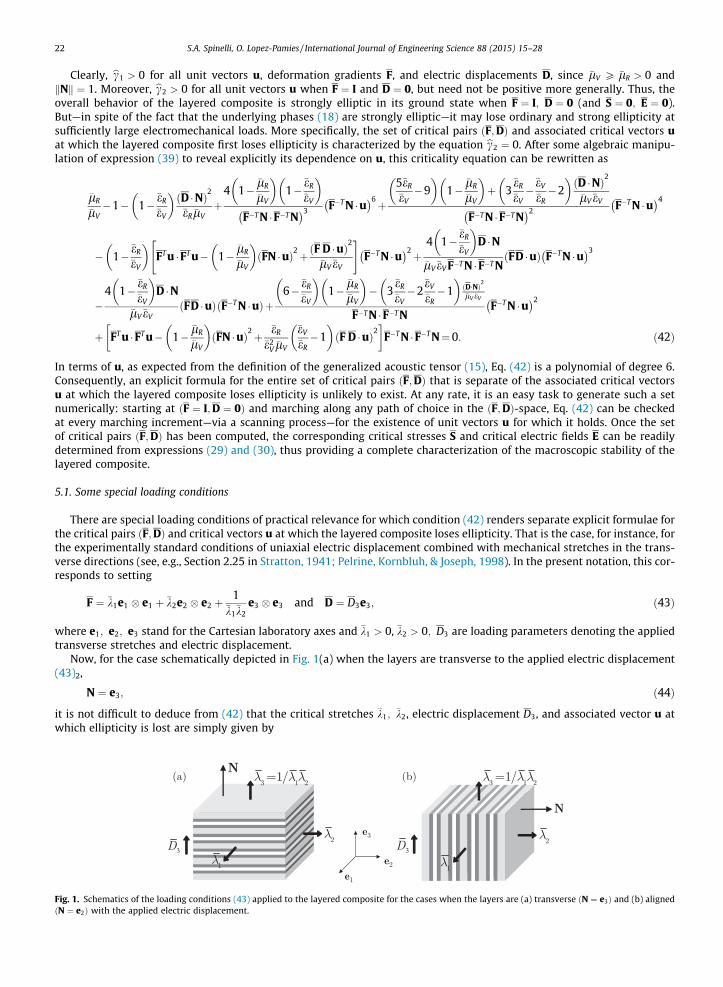
22 S.A. Spinelli, O. Lopez-Pamies / International Journal of Engineering Science 88 (2015) 15–28
Clearly, bc1 > 0 for all unit vectors u, deformation gradients F, and electric displacements D, since �lV P �lR > 0 andkNk ¼ 1. Moreover, bc2 > 0 for all unit vectors u when F ¼ I and D ¼ 0, but need not be positive more generally. Thus, theoverall behavior of the layered composite is strongly elliptic in its ground state when F ¼ I; D ¼ 0 (and S ¼ 0; E ¼ 0).But—in spite of the fact that the underlying phases (18) are strongly elliptic—it may lose ordinary and strong ellipticity atsufficiently large electromechanical loads. More specifically, the set of critical pairs ðF;DÞ and associated critical vectors uat which the layered composite first loses ellipticity is characterized by the equation bc2 ¼ 0. After some algebraic manipu-lation of expression (39) to reveal explicitly its dependence on u, this criticality equation can be rewritten as
Fig. 1.ðN ¼ e2
�lR
�lV�1� 1�
�eR
�eV
� �ðD �NÞ2
�eR �lVþ
4 1��lR
�lV
� �1�
�eR
�eV
� �F�T N �F�T N� 3 F�T N �u
� 6þ
5�eR
�eV�9
� �1�
�lR
�lV
� �þ 3
�eR
�eV�
�eV
�eR�2
� �ðD �NÞ2
�lV�eV
F�T N �F�T N� 2 F�T N �u
� 4
� 1��eR
�eV
� �FT u �FT u� 1�
�lR
�lV
� �ðFN �uÞ2þðF D �uÞ2
�lV�eV
" #F�T N �u� 2þ
4 1��eR
�eV
� �D �N
�lV�eV F�T N �F�T NðFD �uÞ F�T N �u
� 3
�4 1�
�eR
�eV
� �D �N
�lV�eVðFD �uÞðF�T N �uÞþ
6��eR
�eV
� �1�
�lR
�lV
� �� 3
�eR
�eV�2
�eV
�eR�1
� �ðD�NÞ
2
�lV �eV
F�T N �F�T NF�T N �u� 2
þ FT u �FT u� 1��lR
�lV
� �ðFN �uÞ2þ
�eR
�e2V
�lV
�eV
�eR�1
� �ðF D �uÞ2
� �F�T N �F�T N¼0: ð42Þ
In terms of u, as expected from the definition of the generalized acoustic tensor (15), Eq. (42) is a polynomial of degree 6.Consequently, an explicit formula for the entire set of critical pairs ðF;DÞ that is separate of the associated critical vectorsu at which the layered composite loses ellipticity is unlikely to exist. At any rate, it is an easy task to generate such a setnumerically: starting at ðF ¼ I;D ¼ 0Þ and marching along any path of choice in the ðF;DÞ-space, Eq. (42) can be checkedat every marching increment—via a scanning process—for the existence of unit vectors u for which it holds. Once the setof critical pairs ðF;DÞ has been computed, the corresponding critical stresses S and critical electric fields E can be readilydetermined from expressions (29) and (30), thus providing a complete characterization of the macroscopic stability of thelayered composite.
5.1. Some special loading conditions
There are special loading conditions of practical relevance for which condition (42) renders separate explicit formulae forthe critical pairs ðF;DÞ and critical vectors u at which the layered composite loses ellipticity. That is the case, for instance, forthe experimentally standard conditions of uniaxial electric displacement combined with mechanical stretches in the trans-verse directions (see, e.g., Section 2.25 in Stratton, 1941; Pelrine, Kornbluh, & Joseph, 1998). In the present notation, this cor-responds to setting
F ¼ �k1e1 � e1 þ �k2e2 � e2 þ1
�k1�k2
e3 � e3 and D ¼ D3e3; ð43Þ
where e1; e2; e3 stand for the Cartesian laboratory axes and �k1 > 0, �k2 > 0; D3 are loading parameters denoting the appliedtransverse stretches and electric displacement.
Now, for the case schematically depicted in Fig. 1(a) when the layers are transverse to the applied electric displacement(43)2,
N ¼ e3; ð44Þ
it is not difficult to deduce from (42) that the critical stretches �k1; �k2, electric displacement D3, and associated vector u atwhich ellipticity is lost are simply given by
3 3
Schematics of the loading conditions (43) applied to the layered composite for the cases when the layers are (a) transverse ðN ¼ e3Þ and (b) alignedÞ with the applied electric displacement.
3 Cho
S.A. Spinelli, O. Lopez-Pamies / International Journal of Engineering Science 88 (2015) 15–28 23
�k21
�k42 ¼ 1�
�lR
�lVþ D2
3�eR �lV
1��eR
�eV
� �and u ¼ �e2 ð45Þ
if �k1 > �k2, and by
�k41
�k22 ¼ 1�
�lR
�lVþ D2
3�eR �lV
1��eR
�eV
� �and u ¼ �e1 ð46Þ
if, on the other hand, �k1 < �k2. Furthermore, for the case schematically depicted in Fig. 1(b) when the layers are aligned3 withthe applied electric displacement (43)2,
N ¼ e2; ð47Þ
the critical stretches �k1; �k2, electric displacement D3, and associated vector u can be shown to be given by
�k21
�k42 ¼ 1�
�lR
�lV
� ��1
þ D23
�lV�eV1�
�eR
�eV
� �1�
�lR
�lV
� ��1
and u ¼ �e3 ð48Þ
if �k41
�k22 > 1þ D2
3�lV �eV
1� �eR�eV
� �, whereas they are given by
�k21
�k22
¼ 1��lR
�lVand u ¼ �e1 ð49Þ
if, on the other hand, �k41
�k22 < 1þ D2
3�lV �eV
1� �eR�eV
� �. The more general case when the layers are not transverse nor aligned with the
applied electric displacement does not seem to admit separate results for the critical loading �k1, �k2; D3 and associated vectoru. Howbeit, as explained above, it is straightforward to carry out such calculations numerically.
For the case of two phases ðM ¼ 2Þ and plane-strain loading conditions ð�k1 ¼ 1Þ, the ‘‘macroscopic failure surfaces’’ de-fined by (45)1 and (48)1 reduce to those found earlier by Bertoldi and Gei (2011) and Rudykh and deBotton (2011). If, in addi-tion, no electric displacement is applied ðD3 ¼ 0Þ, these surfaces reduce further to the classical result of Triantafyllidis andMaker (1985).
6. The F and E formulation
Depending on the specific problem at hand, it may be more convenient to utilize the Lagrangian electric field E as theindependent electric variable instead of D. In the sequel, for the sake of completeness, we summarize the explicit results gen-erated in Sections 4 and 5 for ideal dielectric layered composites in terms of this alternative variable.
The macroscopic response. By introducing the partial Legendre transform
W� ðF;EÞ ¼ �supD
fD � E�WðF;DÞg ¼
�lV
2½F � F� 3� �
�lV � �lR
2FN � FN� 1
F�T N � F�T N
� ��
�eV
2F�T E � F�T Eþ
�eV � �eR
2F�T E � F�T N� 2
F�T N � F�T Nif J ¼ 1
þ1 otherwise
8>>>>>>><>>>>>>>:ð50Þ
of the effective free energy function (26), it follows that the macroscopic first Piola–Kirchhoff stress S and electric displace-ment field D for the layered composite with M ideal elastic dielectric phases can be written in terms of the macroscopicdeformation gradient F and electric field E simply as
S ¼ @W�
@F� qF�T ¼ �lV F� qF�T � ð�lV � �lRÞFN� Nþ �eV F�T E� F�1F�T E
þ�lV � �lR þ ð�eV � �eRÞðF�T E � F�T NÞ2
F�T N � F�T N� 2 F�T N� F�1 F�T N� ð
�eV � �eRÞF�T E � F�T NF�T N � F�T N
F�T E� F�1F�T Nþ F�T N� F�1F�T E �
ð51Þ
and
D ¼ � @W�
@E¼ �eV F�1F�T E� ð
�eV � �eRÞF�T E � F�T NF�T N � F�T N
F�1F�T N; ð52Þ
where, again, the parameters �lV ; �lR, �eV ; �eR are given by expressions (25), (21) and (22) and the scalar q in (51) denotes theLagrange multiplier associated with the overall incompressibility constraint. As for the F and D version of the result, corre-
osing N ¼ e1 is of course equivalent to choosing N ¼ e2.
24 S.A. Spinelli, O. Lopez-Pamies / International Journal of Engineering Science 88 (2015) 15–28
sponding expressions for the Cauchy stress T, Eulerian electric displacement d, and polarization �p follow trivially from theconnections T ¼ SFT , d ¼ FD, and �p ¼ d� e0F�T E.
In terms of the standard invariants
I1 ¼ F � F; I2 ¼ F�T � F�T ; I4 ¼ FN � FN; I5 ¼ FT FN � FT FN;
I�6 ¼ E � E; I�7 ¼ F E � F E; I�8 ¼ FT F E � FT F E;
I�9 ¼ E � N; I�10 ¼ FE � FN; ð53Þ
it is interesting to recognize that the finite branch of the effective free energy function (50) reads as
W�ðF;EÞ ¼�lV
2½I1 � 3� �
�lV � �lR
2I4 �
1I2 � I1I4 þ I5
� ��
�eV
2I2I�6 � I1I�7 þ I�8 �
þð�eV � �eRÞ I1I4I�6 þ I1I�7 � I2I�6 � I2I�29 � I4I�7 � I5I�6 � I�8 þ I�210
�2
8½I2 � I1I4 þ I5�I�29
; ð54Þ
which, much like its F and D counterpart (28), is not of the separable form W� ¼WelasðI1; I2; I4; I5Þ þW�elec I�6; I
�7; I�8; I�9; I�10
� .
What is more, the functional dependence on the electric invariants I�6 through I�10 is admittedly cumbersome. This suggeststhat the standard set of invariants (53) may not be the most appropriate choice to model transversely isotropic elastic dielec-trics (see, e.g., Bustamante, 2009). The alternative set
I1 ¼ F � F; I2 ¼ F�T � F�T ; I4 ¼ FN � FN; I5 ¼ FT FN � FT FN;
J�6 ¼ E � E; J�7 ¼ F�T E � F�T E; J�8 ¼ F�1F�T E � F�1F�T E;
J�9 ¼ E �N; J�10 ¼ F�T E � F�T N ð55Þ
may prove more appropriate, as it leads to the more compact form
W�ðF;EÞ ¼�lV
2½I1 � 3� �
�lV � �lR
2I4 �
1I2 � I1I4 þ I5
� ��
�eV
2J�7 þ
ð�eV � �eRÞJ�210
2 I2 � I1I4 þ I5 � : ð56Þ
Macroscopic stability. Making use of expression (52) in Eq. (42) allows to rewrite the criticality condition for the loss ofellipticity of the layered composite in terms of the electric field E instead of D. The result reads as
�lR
�lV� 1� 1�
�eR
�eV
� ��eR F�T E � F�T N� 2
�lVþ
4 1��lR
�lV
� �1�
�eR
�eV
� �F�T N � F�T N� 3 F�T N � u
� 6
þ
5�eR
�eV� 9
� �1�
�lR
�lV
� �þ 3
�e2R
�e2V
� 2�eR
�eV� 1
� ��eV F�T E � F�T N� 2
�lV
F�T N � F�T N� 2 F�T N � u
� 4
� 1��eR
�eV
� �FT u � FT u� 1�
�lR
�lV
� �ðFN � uÞ2 þ
�eV F�T E � u� 2
�lV
" #F�T N � u� 2
þ 2�eR
�lV
�eV
�eR�
�eR
�eV
� �F�T E � F�T N�
F�T E � u� F�T N � u
� 2
F�T N � F�T N� 1
" #F�T N � u�
þ6�
�eR
�eV
� �1�
�lR
�lV
� �� 4
�e2R
�e2V
� 3�eR
�eV� 1
� ��eV F�T E � F�T N� 2
�lV
F�T N � F�T NF�T N � u� 2
þ FT u � FT u� 1��lR
�lV
� �ðFN � uÞ2 þ
�eR
�lV
�eV
�eR� 1
� �F�T E � u� 2
� �F�T N � F�T N ¼ 0: ð57Þ
For electromechanical loadings analogous to (43) with
F ¼ �k1e1 � e1 þ �k2e2 � e2 þ1
�k1�k2
e3 � e3 and E ¼ E3e3; ð58Þ
the general condition (57) renders results for the critical pairs ðF;EÞ that are separate from the associated critical vectors u.Indeed, for the case with N ¼ e3 when the layers are transverse to the applied electric field, it follows from (57) that the crit-ical stretches �k1; �k2, electric field E3, and associated vector u at which the layered composite loses ellipticity under loadingconditions of the form (58) are given by
S.A. Spinelli, O. Lopez-Pamies / International Journal of Engineering Science 88 (2015) 15–28 25
�k21
�k42 ¼ 1�
�lR
�lVþ
�eR�k4
1�k4
2E23
�lV1�
�eR
�eV
� �and u ¼ �e2 ð59Þ
if �k1 > �k2, and by
�k41
�k22 ¼ 1�
�lR
�lVþ
�eR�k4
1�k4
2E23
�lV1�
�eR
�eV
� �and u ¼ �e1 ð60Þ
if �k1 < �k2. Similarly, for the case with N ¼ e2 when the layers are aligned with the applied electric field, it follows from (57)that the critical stretches �k1; �k2, electric field E3, and associated vector u at which ellipticity is lost are given by
�k21
�k42 ¼ 1�
�lR
�lV
� ��1
þ�eV
�k41�k4
2E23
�lV1�
�eR
�eV
� �1�
�lR
�lV
� ��1
and u ¼ �e3 ð61Þ
if �k41
�k22 > 1þ
�k41
�k42E2
3�lVð�eV � �eRÞ, whereas they are given by
�k21
�k22
¼ 1��lR
�lVand u ¼ �e1 ð62Þ
if �k41
�k22 < 1þ
�k41
�k42E2
3�lVð�eV � �eRÞ.
7. Concluding remarks
The exact homogenization results (28), (54) and (56) provide insight into the identification of the invariants that domi-nate the effective free energy functions of elastic dielectrics with transversely isotropic microstructures. Indeed, when usingthe electric displacement field D as the independent electric variable, the result (28) suggests that the dominant electricinvariants are simply the standard I7 ¼ FD � FD ¼ d � d and I9 ¼ D � N ¼ d � F�T N. When using the electric field E as theindependent electric variable, on the other hand, the result (54) appears to suggest that all standard electric invariants(53)5–(53)10 are required and equally important in the modeling of transversely isotropic elastic dielectrics. Rewriting theeffective free energy function in the form (56) reveals, however, that only the alternative invariantsJ�7 ¼ F�T E � F�T E ¼ �e � �e and J�10 ¼ F�T E � F�T N ¼ e � F�T N may be of importance. Further studies of elastic dielectrics withricher anisotropic microstructures are under way to corroborate these initial findings (Lopez-Pamies, 2014).
While only results for the onset of macroscopic instabilities have been reported here, the results (23) and (24) for the localdeformation gradient and electric displacement fields within each of the phases in the layered composite allow to readilycompute the onset of other types of instabilities. These include geometric instabilities of microscopic wavelengths (forthe case when the phases are periodically distributed), as well as material instabilities such as cavitation, debonding, andelectric breakdown (see, e.g., Lopez-Pamies, Nakamura, & Idiart, 2011; Michel, Lopez-Pamies, Ponte Castañeda, & Trian-tafyllidis, 2010). Focusing on the latter, for instance, electric breakdown is often presumed to initiate when the magnitudeof the electric field at a material point reaches a critical value, Ecr say (see, e.g., Moscardo, Zhao, Suo, & Lapusta, 2008; Plante& Dubowsky, 2006). By combining the results (52) and (24), the local electric field within each of the phases r ¼ 1;2; . . . ;M inthe layered composite can be simply written as
EðrÞ ¼ Eþ�lR
lðrÞ� 1
� �ðE � NÞNþ
�eR
eðrÞ�
�lR
lðrÞ
� �F�T E � F�T NF�T N � F�T N
N: ð63Þ
Thus, the onset of electric breakdown in the layered composite could be readily computed by monitoring failure of the con-ditions kEðrÞk < Ecr for all r ¼ 1;2; . . . ;M.
We conclude by remarking that the results (26) and (42)—or equivalently (50) and (57)—can be utilized to shed light onthe intricate effects that interphases can have on the macroscopic response and stability of dielectric elastomer composites(Lewis, 2004; Roy et al., 2005). To see this, it suffices to consider the case of a three-phase layered composite ðM ¼ 3Þ wherelayers of material r ¼ 1 are contiguous only to layers of material r ¼ 3 sandwiching layers of material r ¼ 2, in such a mannerthat material r ¼ 3 acts as an interphase between materials r ¼ 1 and r ¼ 2. Because the results (26) and (42) depend on theshear modulus lð3Þ and permittivity eð3Þ of the interphase via the arithmetic and harmonic averages (25), (21) and (22), largeor small values of lð3Þ and eð3Þ can have a substantial effect on these results even when the volume fraction cð3Þ0 of the inter-phase is small. The interested reader is referred to Bertoldi and Lopez-Pamies (2012) for a parametric analysis of the effectsof lð3Þ and cð3Þ0 in the purely mechanical context.
Acknowledgments
This work was supported by the National Science Foundation through the CAREER Grant CMMI–1219336.
26 S.A. Spinelli, O. Lopez-Pamies / International Journal of Engineering Science 88 (2015) 15–28
Appendix A. Derivation of the ellipticity conditions
In this appendix, we provide a brief derivation of the ellipticity conditions (13) and (14) and (16) and (17) for elasticdielectric presented in Section 3. Before proceeding with the technical details, it is fitting to mention that a condition equiv-alent to (14) for the mathematically identical problem of magnetoelasticity was apparently first put forward by Kankanalaand Triantafyllidis (2004). A condition equivalent to (17), also within the problem of magnetoelasticity, was later given byDestrade and Ogden (2011) for incompressible materials. This latter condition has been recently adapted for elastic dielec-trics by Bertoldi and Gei (2011) and Rudykh and deBotton (2011) for the special case of plane-strain loading conditions.
When describing the constitutive response of an elastic dielectric by its ‘‘total’’ free energy function4 W ¼WðF;DÞ, asintroduced by Dorfmann and Ogden (2005), the conservation of momentum and Maxwell equations governing its incrementalquasi-static response at finitely deformed states can be expediently written in updated Lagrangian form as (Ogden, 2009)
4 The
div _S ¼ 0; curl _E ¼ 0; div _D ¼ 0: ð64Þ
Here, the div and curl operators are with respect to x, and the infinitesimal increments in the first Piola–Kirchhoff stress _Sand Lagrangian electric field _E are given in component form by
_Sij ¼ Lijkl _xk;l þMijk_Dk; _Ei ¼Mjki _xj;k þ Bij
_Dj; ð65Þ
in terms of the infinitesimal increments in the deformation _x and Lagrangian electric displacement _D, where
Lijkl ¼ J�1FjaFlb@2W
@Fia@FkbðF;DÞ;
Mijk ¼ FjaF�1bk
@2W@Fia@Db
ðF;DÞ;
Bij ¼ JF�1ai F�1
bj@2W
@Da@DbðF;DÞ ð66Þ
stand for the incremental moduli.In order to deduce the conditions of ordinary and strong ellipticity—akin to the purely mechanical problem (see, e.g., Hill,
1979; Chapter 6.2.7 in Ogden, 1997 and references therein)—we now consider the underlying configuration in the incremen-tal problem (64) to be uniform, with homogeneous deformation gradient F and electric displacement field D, and seek solu-tions of the form
_x ¼ vf ðu � xÞ; _D ¼ wgðu � xÞ; ð67Þ
where u; v; w are constant unit vectors while f and g are scalar-valued functions of their argument. Direct use of expres-sions (67) allows to rewrite Eq. (64) as
Kvf 00 þ Rwg0 ¼ 0; bI½RTvf 00 þBw g0� ¼ 0; bIw ¼ w; ð68Þ
where we have introduced the acoustic tensor K and electro-acoustic tensor R, given in component form by
Kik ¼ Lijklujul; Rik ¼Mijkuj; ð69Þ
and made use of the notation f 00 ¼ d2f ðsÞ=ds2, g0 ¼ dgðsÞ=ds, and
bI ¼ I� u� u: ð70ÞSolving Eqs. (68)2 and (68)3 for w yields
w ¼ � 2
ðtr bBÞ2 � tr bB2½ðtr bBÞbI � bB�RTv
f 00
g0; ð71Þ
where
bB ¼ bIBbI: ð72ÞSubstituting (71) in (68)1 yields in turn the following equation for v:
Cðu; F;DÞv ¼ 0; ð73Þ
where
Cðu; F;DÞ ¼ K� 2
ðtr bBÞ2 � tr bB2R½ðtr bBÞbI � bB�RT ð74Þ
use of bars over the variables W ; F; D; S; E to indicate macroscopic quantities is unnecessary here, and hence dropped for simplicity.
S.A. Spinelli, O. Lopez-Pamies / International Journal of Engineering Science 88 (2015) 15–28 27
corresponds to the generalized acoustic tensor of the elastic dielectric. Clearly, non-trivial solutions of the form (67) to theincremental problem (64) cannot exist if
det Cðu; F;DÞ– 0 ð75Þ
for all unit vectors u and all F; D. Noting that CT ¼ C, a stronger condition that prevents non-trivial solutions of the form (67)is given by
v � Cðu; F;DÞv > 0 ð76Þ
for all unit vectors u; v and all F, D. Conditions (75) and (76) constitute, respectively, the conditions of ordinary and strongellipticity for unconstrained elastic dielectrics.
Incompressible materials. For the case of incompressible materials, when the free energy function of the elastic dielectric isof the constrained form W ¼WðF;DÞ if J ¼ 1 and W ¼ þ1 otherwise, the vector v in (67) is constrained according to
bIv ¼ v; ð77Þand the incremental Eq. (64) specialize further to
bI½Kvf 00 þ Rwg0� ¼ 0; bI½RTvf 00 þBwg0� ¼ 0; bIw ¼ w ð78Þwith J ¼ 1 in (66). Substituting relations (77) and (78)3 in Eq. (78)2 and then solving for w leads to the explicit result
w ¼ � 2
ðtr bBÞ2 � tr bB2½ðtr bBÞbI � bB� bRTv
f 00
g0; ð79Þ
where bR ¼ bI RbI and bB is recalled to be given by (72). Substituting (77) and (79) in (78)1 leads in turn to the following equa-tion for v:
bCðu; F;DÞv ¼ 0; ð80Þwhere
bCðu; F;DÞ ¼ bK � 2
ðtr bBÞ2 � tr bB2
bR½ðtr bBÞbI � bB� bRT ð81Þ
with bK ¼ bI KbI. Expression (81) corresponds to the generalized acoustic tensor of the incompressible elastic dielectric. Clearly,bCT ¼ bC and thus bC has two non-trivial real eigenvalues on the two-dimensional space normal to u. Since, according to (77),the vector v also lies on the two-dimensional space normal to u, it follows from (80) that non-trivial solutions of the local-ization type (67) to the incremental problem (64) cannot exist if
ðtr bCðu; F;DÞÞ2� tr bC2ðu; F;DÞ – 0 ð82Þ
for all unit vectors u and all F with J ¼ 1, D. A stronger condition that prevents the existence of non-trivial solutions is givenby
v � bCðu; F;DÞv > 0 ð83Þ
for all unit vectors u; v such that u � v ¼ 0 and all F with J ¼ 1; D. Conditions (82) and (83) constitute, respectively, the con-ditions of ordinary and strong ellipticity for incompressible elastic dielectrics.
References
Bertoldi, K., & Gei, M. (2011). Instabilities in multilayered soft dielectrics. Journal of the Mechanics and Physics of Solids, 59, 18–42.Bertoldi, K., & Lopez-Pamies, O. (2012). Some remarks on the effect of interphases on the mechanical response and stability of fiber-reinforced elastomers.
Journal of Applied Mechanics, 79, 031023.Bustamante, R. (2009). Transversely isotropic non-linear electro-active elastomers. Acta Mechanica, 206, 237–259.deBotton, G., Tevet-Deree, L., & Socolsky, E. A. (2007). Electroactive heterogeneous polymers: Analysis and applications to laminated composites. Mechanics
of Advanced Materials and Structures, 14, 13–22.Destrade, M., & Ogden, R. W. (2011). On magneto-acoustic waves in finitely deformed elastic solids. Mathematics and Mechanics of Solids, 16, 594–604.Dorfmann, A., & Ogden, R. W. (2005). Nonlinear electroelasticity. Acta Mechanica, 174, 167–183.Geymonat, G., Müller, S., & Triantafyllidis, N. (1993). Homogenization of nonlinearly elastic materials, microscopic bifurcation and macroscopic loss of rank-
one convexity. Archive for Rational Mechanics and Analysis, 122, 231–290.Hill, R. (1972). On constitutive macrovariables for heterogeneous solids at finite strain. Proceedings of the Royal Society of London Series A, 326, 131–147.Hill, R. (1979). On the theory of plane strain in finitely deformed compressible materials. Mathematical Proceedings of the Cambridge Philosophical Society, 86,
161–178.Huang, C., Zhang, Q. M., Li, J. Y., & Rabeony, M. (2005). Colossal dielectric and electromechanical responses in self-assembled polymeric nanocomposites.
Applied Physics Letters, 87, 182901.Kankanala, S. V., & Triantafyllidis, N. (2004). On finitely strained magnetorheological elastomers. Journal of the Mechanics and Physics of Solids, 52,
2869–2908.Kofod, G., Sommer-Larsen, P., Kornbluh, R., & Pelrine, R. (2003). Actuation response of polyacrylate dielectric elastomers. Journal of Intelligent Material
Systems and Structures, 14, 787–793.
28 S.A. Spinelli, O. Lopez-Pamies / International Journal of Engineering Science 88 (2015) 15–28
Lewis, T. J. (2004). Interfaces are the dominant feature of dielectrics at the nanometric level. IEEE Transactions on Dielectrics and Electrical Insulation, 11,739–753.
Lopez-Pamies, O. (2014). Elastic dielectric composites: Theory and application to particle-filled ideal dielectrics. Journal of the Mechanics and Physics of Solids,64, 61–82.
Lopez-Pamies, O., Nakamura, T., & Idiart, M. I. (2011). Cavitation in elastomeric solids: II—Onset-of-cavitation surfaces for Neo-Hookean materials. Journal ofthe Mechanics and Physics of Solids, 59, 1488–1505.
Michel, J. C., Lopez-Pamies, O., Ponte Castañeda, P., & Triantafyllidis, N. (2010). Microscopic and macroscopic instabilities in finitely strained fiber-reinforcedelastomers. Journal of the Mechanics and Physics of Solids, 58, 1776–1803.
Moscardo, M., Zhao, X., Suo, Z., & Lapusta, Y. (2008). On designing dielectric elastomer actuators. Journal of Applied Physics, 104, 093503.Ogden, R. W. (1997). Non-linear elastic deformations. Mineola, New York: Dover.Ogden, R. W. (2009). Nonlinear elastic motions superimposed on a finite deformation in the presence of an electromagnetic field. International Journal of
Non-linear Mechanics, 44, 570–580.Pelrine, R., Kornbluh, R., & Joseph, J. P. (1998). Electrostriction of polymer dielectrics with compliant electrodes as a means of actuation. Sensors and Actuators
A, 64, 77–85.Plante, J. S., & Dubowsky, S. (2006). Large-scale failure modes of dielectric elastomer actuators. International Journal of Solids and Structures, 43, 7727–7751.Roy, M., Nelson, J. K., MacCrone, R. K., Schadler, L. S., Reed, C. W., Keefe, R., et al (2005). Polymer nanocomposite dielectrics—The role of the interface. IEEE
Transactions on Dielectrics and Electrical Insulation, 12, 629–643.Rudykh, S., & deBotton, G. (2011). Stability of anisotropic electroactive polymers with application to layered media. Zeitschrift fur Angewandte Mathematik
und Physik, 62, 1131–1142.Stratton, J. S. (1941). Electromagnetic theory. McGraw-Hill.Tian, L., Tevet-Deree, L., deBotton, G., & Bhattacharya, K. (2012). Dielectric elastomer composites. Journal of the Mechanics and Physics of Solids, 60, 181–198.Triantafyllidis, N., & Maker, B. N. (1985). On the comparison between microscopic and macroscopic instability mechanisms in a class of fiber-reinforced
composites. Journal of Applied Mechanics, 52, 794–800.Wissler, M., & Mazza, E. (2007). Electromechanical coupling in dielectric elastomer actuators. Sensors and Actuators A, 138, 384–393.Zhang, S., Huang, C., Klein, R. J., Xia, F., Zhang, Q. M., & Cheng, Z. Y. (2007). High performance electroactive polymers and nano-composites for artificial
muscles. Journal of Intelligent Material Systems and Structures, 18, 133–145.