International Journal of Pharma and Bio Sciences ISSN … · Int J Pharm Bio Sci 2015 April; 6(2): (B) 1126 ... DESIGN OF ENSEMBLES WITH SVM KERNELS FOR DIABETES DATASET ... figure

Int J Pharm Bio Sci 2015 April; 6(2): (B) 1126 - 1139

This article can be downloaded from www.ijpbs.net

B - 1126

Research Article Bioinformatics

International Journal of Pharma and Bio Sciences ISSN

0975-6299

DESIGN OF ENSEMBLES WITH SVM KERNELS FOR DIABETES DATASET

T.LAVANYA

1 AND A.KUMARAVEL

2

1Research Scholar, Department of Computer Science and Engineering Bharath University, Selaiyur, Chennai-

600073, [email protected] 2

Professor and Dean, School of Computing, .Bharath University, Selaiyur, Chennai-600073, India

[email protected]

ABSTRACT

Data mining methods based on support vector machine are attractive to address the curse of dimensionality. The Kernel mapping contributes a unifying frame work for most of the commonly employed models to get the linear planes in the higher dimensional space. In this paper, we prove this approach enhances the accuracy of diabetes data set. We further refine the results with parameter tuning for the selected kernels. The natural question that arises in the case of many such different mappings to choose from, which is the best for a particular problem? The selection can be validated using independent test sets or a variety of data sets and methods of cross validations. KEYWORDS: Ensembles Bagging, Dagging, Multi boost, Ada boost, Support Vector Machine, Kernel functions, Polynomial kernel, Normalized polynomial, Pearson VII function-based, RBF kernel,

*Corresponding author

A.KUMARAVEL

Professor and Dean, School of Computing, .Bharath University,

Selaiyur, Chennai-600073, India



B - 1127

INTRODUCTION

We emphasize the aggregation of multiple learning models with the goal of improving overall accuracy. Most of the algebraic methods like finding simple average, weighted average, simple or weighted sum, product, maximum, minimum, median and procedures like voting methods, majority voting ,weighted majority voting, Borda count ate applied to combine the learning models. Even though the accuracy is expected to increase, it is more difficult to characterize and explain predictions. Data mining research community is confronted with issues of computational constraints like time complexity and data size the non linear kernel of SVM model requires a run time of quadratic in the size of the training set n, thus the training complexity becomes Ω(n

2) [1].A divide and conquer strategy

by aggregating many SVM models, trained on small sub samples of the training set using p classifiers on subsamples of size n/p gives complexity of Ω(n

2/p) [2]. In this paper a novel

architecture for ensemble learning is proposed this architecture is proposed to balance the basic classifiers with individual accuracy and diversity. For this purpose we consider SVM model with different kernels and bounding parameters. Kernel function makes the classification to be carried over in higher dimensional spaces. Inner products are used for construction of the maximal margin hyper-plane. Classification is easier in high dimensional spaces. The exploration and formalization of these concepts have resulted in theory of statistical learning [3].Authors in [4] had shown the improvement by classifiers other than the support vector machine type classifiers by selection of attributes. In this paper, we consider the family of support vector machine type of classifiers in the same direction. Moreover, we do the parameter training with the kernel function applied to support vector machine classifier for further possible accuracy. Medical domain deals with critical data at one or the other example with very fuzzy and ambiguous data values at times. In such context improved accuracy of predictions is essential. Taking decision through wide range of opinions is better than individual decision. In this paper, we prove our approach to enhance the accuracy for diabetes data set.

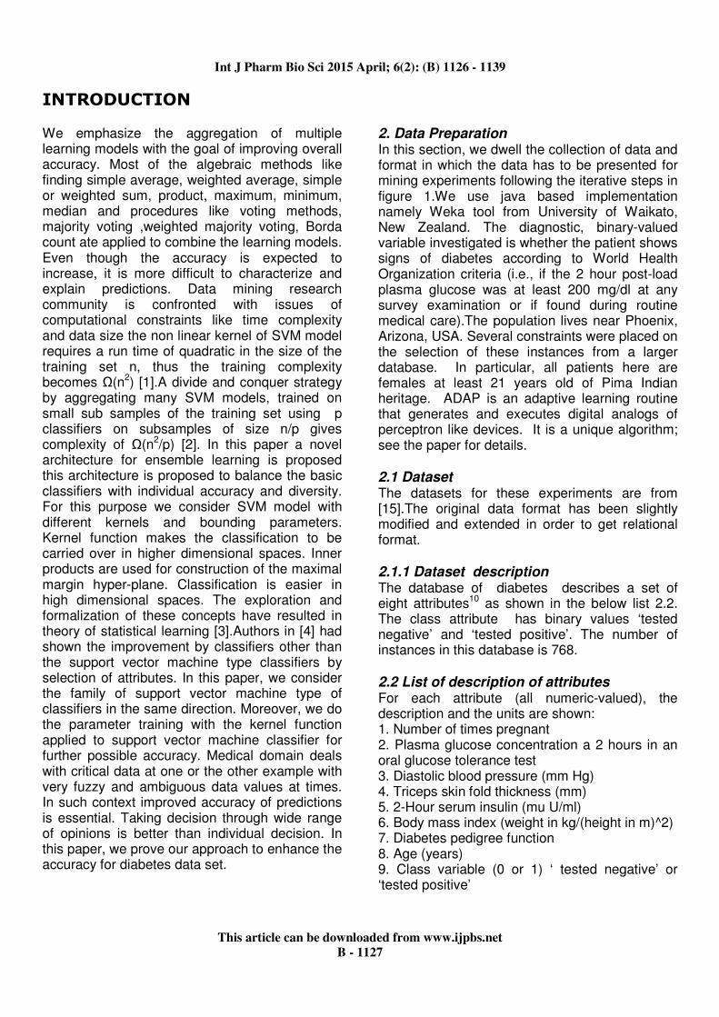
2. Data Preparation In this section, we dwell the collection of data and format in which the data has to be presented for mining experiments following the iterative steps in figure 1.We use java based implementation namely Weka tool from University of Waikato, New Zealand. The diagnostic, binary-valued variable investigated is whether the patient shows signs of diabetes according to World Health Organization criteria (i.e., if the 2 hour post-load plasma glucose was at least 200 mg/dl at any survey examination or if found during routine medical care).The population lives near Phoenix, Arizona, USA. Several constraints were placed on the selection of these instances from a larger database. In particular, all patients here are females at least 21 years old of Pima Indian heritage. ADAP is an adaptive learning routine that generates and executes digital analogs of perceptron like devices. It is a unique algorithm; see the paper for details. 2.1 Dataset The datasets for these experiments are from [15].The original data format has been slightly modified and extended in order to get relational format. 2.1.1 Dataset description The database of diabetes describes a set of eight attributes

10 as shown in the below list 2.2.

The class attribute has binary values ‘tested negative’ and ‘tested positive’. The number of instances in this database is 768. 2.2 List of description of attributes For each attribute (all numeric-valued), the description and the units are shown: 1. Number of times pregnant 2. Plasma glucose concentration a 2 hours in an oral glucose tolerance test 3. Diastolic blood pressure (mm Hg) 4. Triceps skin fold thickness (mm) 5. 2-Hour serum insulin (mu U/ml) 6. Body mass index (weight in kg/(height in m)^2) 7. Diabetes pedigree function 8. Age (years) 9. Class variable (0 or 1) ‘ tested negative’ or ‘tested positive’



B - 1128

2.3 Brief statistical analysis

Attribute number

Mean Standard Deviation

1. 3.8 3.4

2. 120 32.0

3. 69.1 19.4 4. 20.5 16.0

5. 79.8 115.2 6. 32.0 7.9

7. 0.5 0.3

8. 33.2 11.8

3. Methods Description

Figure 1

Base classifier tuning and Mining



B - 1129

Figure1 depicts the architecture of the proposed system for using the support vector methods. These methods are capable of generating models with high accuracy, they are parameterized by kernel functions and few real values (i.e. like ‘c’ value, a typical parameter).The usage of SVM is explained in the following section. 3.1 SVM Classifier The SVM learning model eventually produces a hyper plane separating the classes in the higher dimension space. The extreme points in each class are used to identify the “support vectors” in the given training set and these support vectors uniquely determines the hyper plane. This is obtained by Quadratic optimization algorithms with training points xi and non-zero Lagrangian multipliers αi formulated as follows: Find … such that

Q(α)= is maximized and

(1)

(2) 0 C for all (3.1)

3.1.1The Optimal Separating Hyperplane Consider the problem [16] of separating the set of training vectors belonging to two separate classes,

, , ∈

with a hyper plane, (3.1.1)

The set of vectors is said to be optimally separated by the hyper plane if it is separated without error and the distance between the closest vector to the hyper plane is maximal. There is some redundancy in Equation 3.1.1, and without loss of generality it is appropriate to consider a canonical hyper plane, where the parameters w, b are constrained by,

(3.1.2)

This incisive constraint on the parameterisation is preferable to alternatives in simplifying the formulation of the problem. In words it states that: the norm of the weight vector should be equal to the inverse of the distance, of the nearest point in the data set to the hyper plane. The idea is illustrated in Figure 2, where the distance from the nearest point to each hyper plane is shown.

Figure 2 Canonical Hyper planes



B - 1130

A separating hyper plane in canonical form must satisfy the following constraints, (3.1.3)

The distance d(w, b; x) of a point x from the hyper plane (w, b) is,

(3.1.4)

The optimal hyper plane is given by maximizing the margin, ρ, subject to the constraints of equation 3.1.3. The margin is given by,

(3.1.5)

Hence the hyper plane that optimally separates the data is the one that minimizes

(3.1.6)

It is independent of b because provided Equation 3.1.3 is satisfied (i.e. it is a separating hyperplane) changing b will move it in the normal direction to itself. Accordingly the margin remains unchanged but the hyperplane is no longer optimal in that it will be nearer to one class than the other. To consider how minimising Equation 3.1.6 is equivalent to implementing the SRM principle, suppose that the following bound holds, (3.1.7)

then from Equation 3.1.2 and 3.1.3,

(3.1.8)

Accordingly the hyperplanes cannot be nearer than to any of the data points and intuitively it can be

seen in Figure 3, how this reduces the possible hyperplanes, and hence the capacity.



B - 1131

Figure 3 Constraining the Canonical Hyper planes

The VC dimension, h, of the set of canonical hyper planes in n dimensional space is bounded by (3.1.9)

is given by the saddle point of the Lagrange functional

>+b]-1) (3.1.10)

where α are the Lagrange multipliers. The Lagrangian has to be minimised with respect to w, b and maximised with respect to α ≥ 0. Classical Lagrangian duality enables the primal problem, Equation 3.1.11, to be transformed to its dual problem, which is easier to solve. The dual problem is given by,

(3.1.11)

The minimum with respect to w and b of the Lagrangian, Φ, is given by,

(3.1.12)

Hence from Equations 3.10, 3.11 and 3.12, the dual problem is,

(3.1.13)

and hence the solution to the problem is given by,

(3.1.14)

with constraints,

(3.1.15)

Solving Equation 3.1.14 with constraints Equation 3.1.15 determines the Lagrange multi-pliers, and the optimal separating hyper-plane is given by,

(3.1.17)



B - 1132

where xr and xs are any support vector from each class satisfying, (3.1.17)

The hard classifier is then, (3.1.18)

Alternatively, a soft classifier may be used which linearly interpolates the margin,

where h(z)= (3.1.19)

This may be more appropriate than the hard classifier of Equation 3.1.19, because it produces a real valued output between −1 and 1 when the classifier is queried within the margin, where no training data resides. From the Kuhn-Tucker conditions, [<w, (3.1.20)

and hence only the points x i which satisfy, (3.1.21)

will have non-zero Lagrange multipliers. These points are termed Support Vectors (SV). If the data is linearly separable all the SV will lie on the margin and hence the number of SV can be very small. Consequently the hyper-plane is determined by a small subset of the training set; the other points could be removed from the training set and recalculating the hyper-plane would produce the same answer. Hence SVM can be used to summarise the information contained in a data set by the SV produced. If the data is linearly separable the following equality will hold,

(3.1.22)

Hence from Equation 3.1.9 the VC dimension of the classifier is bounded by, +1 (3.1.23)

and if the training data, x, is normalised to lie in the unit hyper-sphere, (3.1.24)

3.2 Kernel Functions As mentioned in the introduction kernel functions are symmetric and positive definite [17,18,19]. An inner product in feature space has an equivalent kernel in input space,

(3.2.1)

provided certain conditions hold. Since K is a symmetric positive definite function, which satisfies Mercer’s Conditions, (3.2.2)

(3.2.3)



B - 1133

then the kernel represents a legitimate inner product in feature space. Valid functions that satisfy Mercer’s conditions are now given, which unless stated are valid for all real and . We consider

four types kernel Polynomial kernel, Normalized polynomial, Pearson VII function-based, RBF kernels for identifying the variance in the SVM classifiers’ behavior. The following sections describe briefly the methods for kernels and results of such methods are tabulated further.

Figure 4 Visualizing the ‘Linearity’ in the higher dimensional space by Kernel functions

3.2.1 Polynomial kernel

A polynomial mapping is a popular method for non-linear modelling,

(3.4)

(3.5)

The second kernel is usually preferable as it avoids problems with the hessian becoming zero. In machine learning, the polynomial kernel is a kernel function commonly used with support vector machines (SVMs) and other kernelized models, that represents the similarity of vectors (training samples) in a feature space over polynomials of the original variables, allowing learning of non-linear models. Intuitively, the polynomial kernel looks not only at the given features of input samples to determine their similarity, but also combinations of these. In the context of regression analysis, such combinations are known as interaction features. The (implicit) feature space of a polynomial kernel is equivalent to that of polynomial regression, but without the combinatorial blowup in the number of parameters to be learned. When the input features are binary-valued (booleans), then the

features correspond to logical conjunctions of input features. 3.2.2 Normalized Polynomial kernel This is the particular space of polynomial kernel type in 3.2.1.The normalized polynomial kernel K(x,y) = <x,y>/sqrt(<x,x> <y,y>) where <x,y> = PolyKernel(x,y) 3.2.3 Pearson VII Pearson VII function is adopted as an alternative generic kernel function in this study. It might serve as a kind of universal kernel which can replace (by selecting the appropriate parameter setting) the set of commonly applied kernel functions, i.e. the linear, polynomial, Gaussian and Sigmoid kernels. Adopting Pearson VII function as kernel function, it might avoid the case that SVM can’t match data well



B - 1134

if the kind of kernel function of SVM was chosen wrongly. The Pearson VII kernel

function of multi-dimensional input space is given by the following formula

Pearson VII universal kernel function, referred to as PUK in this paper, is used as SVM kernel function. Here it is possible to use the Pearson VII function as a generic kernel which can replace the earlier mentioned set of kernel functions. 3.2.4 Radial basis function kernel A radial basis function (RBF) is a real-valued function whose value depends only on the distance from the origin, so that

or alternatively on the distance from some other point c, called a center, so that

. Any function that satisfies

the property is a radial function.

The norm is usually Euclidean distance, although other distance functions are also possible. For example, a radial function Φ in two dimensions has the form

where φ is a

function of a single non-negative real variable. Radial functions are contrasted with spherical functions, and indeed any decent function on Euclidean space can be decomposed into a series consisting of radial and spherical parts: the solid spherical harmonic expansion. 4 Parameter Training Various values of parameter C in (3.1) determine the performance of SVM classifier. Selecting parameter C is depends on the range of output values. This is a reasonable proposal, but it does not take into account possible effect of outliers in the training data. The parameter C controls the trade-off between the margin and

the size of the slack variables. In practice the parameter C is varied through a wide range of values and the optimal performance assessed using a separate validation set. C is essentially a regularisation parameter, which controls the trade-off between achieving a low error on the training data and minimising the norm of the weights. Tuning C correctly is a vital step in best practice in the use of SVMs, as structural risk minimisation (the key principle behind the basic approach) is partly implemented via the tuning of C. The parameter C enforces an upper bound on the norm of the weights, which means that there is a nested set of hypothesis classes indexed by C. As we increase C, we increase the complexity of the hypothesis class (if we increase C slightly, we can still form all of the linear models that we could before and also some that we couldn't before we increased the upper bound on the allowable norm of the weights). So as well as implementing SVM via maximum margin classification, it is also implemented by the limiting the complexity of the hypothesis class via controlling C. Unfortunately the effort for determining how to select C is not very well developed at the moment, so most people tend to use cross-validation.



B - 1135

5 Design of Ensembles

6 Experimental Setup The experiment based on diabetes dataset is carried out to generate the various levels of accuracy as tabulated. Polynomial kernel is applied for the datasets O,F with original attributes and filtered attributes. O= Pregnant, Plasma, blood pressure , skin, serum, Body mass ,Diabetes, Age F= Plasma, Body mass, Diabetes, Age . Table 1 shows the accuracy of polynomial kernel obtained by varying the parameter C values.

Table 1

Performance of Polynomial kernel

Ada Boost (Base Classifier:SVM)

Kernel Type C Time Taken Accuracy

Polynomial kernel

1 0.65 77.3438 2 0.46 77.474

3 0.45 77.474 4 0.6 77.7344

5 0.57 77.6042

6 0.61 77.6042

7 0.66 77.3438 8 0.72 77.2135

9 0.49 77.3438 10 0.8 77.3438

Table 2

Performance of Normalized polynomial



Normalized polynomial

1 26.65 69.9219 2 26.5 70.7031

3 29.65 69.6615

4 27.51 71.0938 5 27.65 71.224

6 27.99 70.5729

7 28.71 70.5729 8 28.27 70.0521

9 29.19 70.0521

10 29.82 70.5729



B - 1136

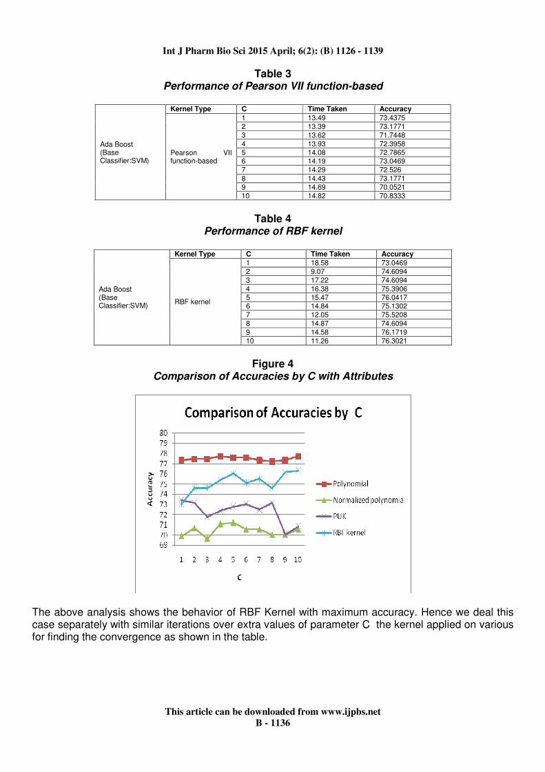
Table 3 Performance of Pearson VII function-based



Pearson VII function-based

1 13.49 73.4375

2 13.39 73.1771

3 13.62 71.7448

4 13.93 72.3958 5 14.08 72.7865 6 14.19 73.0469

7 14.29 72.526

8 14.43 73.1771

9 14.69 70.0521

10 14.82 70.8333

Table 4

Performance of RBF kernel



RBF kernel

1 18.58 73.0469

2 9.07 74.6094

3 17.22 74.6094

4 16.38 75.3906 5 15.47 76.0417 6 14.84 75.1302

7 12.05 75.5208

8 14.87 74.6094

9 14.58 76.1719

10 11.26 76.3021

Figure 4

Comparison of Accuracies by C with Attributes

The above analysis shows the behavior of RBF Kernel with maximum accuracy. Hence we deal this case separately with similar iterations over extra values of parameter C the kernel applied on various for finding the convergence as shown in the table.



B - 1137

Adaboost M1 (Base Classifier:SVM)


RBF kernel

-5 0.06 65.1042

-4 0.06 65.1042

-3 0.06 65.1042

-2 0.06 65.1042

-1 0.07 65.1042

0 0.25 65.1042

1 18.58 73.0469

2 9.07 74.6094

3 17.22 74.6094

4 16.38 75.3906

5 15.47 76.0417

6 14.84 75.1302

7 12.05 75.5208

8 14.87 74.6094

9 14.58 76.1719

10 11.26 76.3021

50 4.79 77.3438 100 4.58 77.3438

200 6.3 77.3438

300 6.17 77.474 400 9.41 77.474

500 14.93 77.6042

Bagging (Base Classifier:SVM)


RBF kernel

1 7.04 65.1042

2 7.75 65.1042

3 6.34 65.1042

4 6.32 67.3177

5 4.77 69.1406

6 4.49 72.9167

7 4.57 73.6979

8 4.68 74.8698

9 3.88 75.651

10 3.84 76.3021

Dagging (Base Classifier:SVM)


RBF kernel

1 0.18 65.1042

2 0.15 65.1042

3 0.16 65.1042

4 0.16 65.1042

5 0.15 65.1042

6 0.15 65.1042

7 0.16 65.1042

8 0.16 65.1042

9 0.16 65.1042

10 0.15 65.1042

MultiBoostAB (Base Classifier:SVM)


RBF kernel

1 15.79 73.4375

2 14.56 73.4375 3 13.86 73.8281

4 13.23 73.5677

5 12.83 75.2604 6 14.9 74.2188

7 13.1 75.1302

8 12.2 75.5208

9 12.43 76.3021

10 12.13 76.8229



B - 1138

Figure 5 Comparison of Accuracies by C for RBF kernel with different Ensembles

Only the Bagging ensemble shows the behavior of increasing accuracy on the variation of the parameter C, upper bound for the coefficients of the optimization in the SVM model acting as the base classifier. Whereas the other ensembles, multi classifiers like Adaboost and Mulitboost, have accuracy with negligible variations of the parameter C. Dagging maintains constant, almost everywhere.

4.1 RESULTS

The four Support Vector Models with Polynomial kernel normalized polynomial, Pearson VII function-based, RBF kernel and have been compared to know which is more accurate and suitable in classification of diabetes patients. Cross validation training with

10 folds is applied and obtained accuracy for the selected kernel functions.

4.2 CONCLUSION

Ensemble design by Support Vector Models has been explored and the effect of the parameters of these models is observed for the diabetes data set.

ACKNOWLEDGEMENT

Authors would like to thank management and research division of Bharath University, India for their support and encouragement for this research work.

REFERENCES

1. Leon Bottou., chih-jen. “Support vector

machine solvers Large scale kernel machines”, Cambridge,MA,USA, MIT Press. 301-320, (2007).

2. Nikolas List., Hans Ulrich Simon. “ SVM optimization and steepest-descent line search”, Proceedings of the 22 nd Annual Conference of Computational Learning Theory, 2009.

3. V. Vapnik. Estimation of Dependences Based on Empirical Data [in Russian]. Nauka, Moscow, 1979.(English translation: Springer Verlag, New York, 1982).

4. [D.Udhayakumarapandian.,RM.Chandrasekaran., and A.Kumaravel “A Novel Subset Selection For Classification Of Diabetes Dataset By Iterative Methods” Int



B - 1139

J Pharm Bio Sci ,5 (3) : (B) 1 – 8, July(2014)

5. A.Kumaravel., Udhayakumarapandian.D.,Consruction Of Meta Classifiers For Apple Scab Infections , Int J Pharm Bio Sci, 4(4): (B) 1207 – 1213, Oct(2013)

6. A.Kumaravel., Pradeepa.R., Efficient molecule reduction for drug design by intelligent search methods.Int J Pharm Bio Sci, 4(2): (B) 1023 – 1029,Apr (2013)

7. D.Udhayakumarapandian.,RM.Chandrasekaran., andA.Kumaravel “Enhancing The Accuracy 0f Svm Classifiers With Kernel And Parameter Training” Int J Pharm Bio Sci , 6(2): (B) 204 - 217, April(2015) (In press)

8. https://www.waset.org/journals/waset/v68/v68-21.pdf world academy of science, engineering and technology, 2012.

9. H.Dunham, Data Mining, Introductory and Advanced Topics, Prentice Hall, ISBN-10: 0130888923 Published 08/22/2002.

10. Source about weka http://www.cs.waikato.ac.nz/ml/weka/ downloaded on 3rd august 2014

11. L. Breiman, “ Random Forests,”in Machine Learning, vol. 45, pp. 5-32, 2001.

12. Dietterich T. G., Jain, A., Lathrop, R., Lozano-Perez, T. A comparison of dynamic reposing and tangent distance for drug activity prediction.Advances in Neural Information Processing Systems, 6. San Mateo, CA: Morgan Kaufmann. 216—223, (1994).

13. A.Stensvand, T. Amundsen, L. Semb, D.M. Gadoury, and R.C. Seem.. Ascospore release and infection of apple leaves by conidia and ascospores of

Venturia inaequalis at low temperatures. Phytopathology 87:1046-1053, 1997.

14. Website for attribute description http://archive.ics.uci.edu/ml/machine-learning databases/pima-indians-diabetes., accessed on 3rd august 2014.

15. Bal,.Bioinformatics-principles and applications.Tata McGraw-Hill Publishing company Ltd New Delhi Hp.(2005).

16. Bo.Th ., Jonassen, New feature subset selection procedures for classification of expression profiles.Genome Biology 3:research 00170.-0017.11 I,(2002)

17. Khalid AA Abakar & Chongwen Yua., Performance of SVM based on PUK kernel in comparison to SVM based on RBF kernel in prediction of yarn tenacity, Indian Journal of Fibre & Textile Research, Vol. 39: (B) 55-59, March (2014).

18. Steve R., Gunn. Support Vector Machines for Classification and Regression Technical Report., Faculty of Engineering, Science and Mathematics School of Electronics and Computer Science .,10 May 1998.

19. F. Girosi., An equivalence between sparse approximation and Support Vector Machines.A.I. Memo 1606, MIT Artificial Intelligence Laboratory, 1997.

20. N. Heckman., The theory and application of penalized least squares methods or reproducing kernel hilbert spaces made easy, 1997.

21. G. Wahba. Spline Models for Observational Data. Series in Applied Mathematics,Vol. 59, SIAM, Philadelphia, 1990.

Documents

International Journal of Pharma and Bio Sciences ISSN … · Int J Pharm Bio Sci 2015 April; 6(2): (B) 1126 ... DESIGN OF ENSEMBLES WITH SVM KERNELS FOR DIABETES DATASET ... figure