International Journal of Pure and Applied Mathematics ... · PDF fileInternational Journal of Pure and Applied Mathematics |||||{Volume 65 No. 3 2010, 297-310 EVALUATION OF BETA-FUNCTION

International Journal of Pure and Applied Mathematics————————————————————————–Volume 65 No. 3 2010, 297-310

EVALUATION OF BETA-FUNCTION B-SPLINES, I:

LOCAL MONOMIAL BASES

Lubomir T. Dechevsky

R&D Group for Mathematical ModellingNumerical Simulation and Computer Visualization

Faculty of TechnologyNarvik University College

2, Lodve Lange’s Str., P.O. Box 385, N-8505, Narvik, NORWAY

e-mail: [email protected]: http://ansatte.hin.no/ltd/

Abstract: This is the first one of a sequence of three papers addressingthe evaluation of Beta function B-splines (BFBS) earlier introduced and stud-ied in [2, 4, 3]. BFBS are a special case of generalized expo-rational B-splines(GERBS) [2, 4], and are a practically important instance of smooth GERBSwhich are not infinitely smooth true expo-rational B-splines (ERBS) [1, 5].Compared to ERBS, BFBS exhibit similar properties, cf. [5, 3], but with morelimited range, due to the polynomial nature of BFBS compared to the exponen-tial nature of ERBS. On the other hand, the integrals in the definition of BFBScan be solved exactly in elementary functions, and the resulting representa-tion is computationally efficient, while with ERBS the respective integrals arespecial functions which can be computed efficiently, yet approximately. Thismakes BFBS more applicable than ERBS, e.g., in topics related to refinement,subdivision, multiresolution and other multilevel techniques.

The present sequence of three papers is dedicated to the derivation of ex-plicit representations of BFBS yielding computationally efficient explicit for-mulae for evaluation of BFBS in terms of polynomial bases used in data in-terpolation, data fitting and geometric modelling, as well as in the design ofmultilevel constructions such as, e.g., multiwavelets. This is the first paperof the sequence, and here we derive a representation of BFBS in terms of lo-cal monomial bases. This is an essentially interpolatory representation; in thesecond article of the sequence, a Bezier type representation of BFBS will be

Received: January 28, 2010 c© 2010 Academic Publications

298 L.T. Dechevsky

considered, which is suitable for geometric modelling and data fitting; the thirdand last paper of the sequence will be dedicated to a representation in globalmonomial bases, suitable for use, e.g., in relevance to certain operational calculi.

AMS Subject Classification: 33B15, 33B20, 41A15, 65D05, 33F05, 41A30,65D07, 65D10, 65D20, 65D30Key Words: spline, B-spline, exponential, rational, expo-rational, general-ized, polynomial, special function, Gamma-function, Euler Beta-function, com-plete, incomplete, Beta-function B-spline, monomial basis, Bernstein basis, lo-cal, global, interpolation, fitting, geometric modelling, operational calculus

1. Introduction

Expo-rational B-splines (ERBS) were introduced in [1] and their propertieswere studied in considerable detail in [5]. Applications of ERBS in geometricmodelling with parametric curves and tensor-product surfaces were consideredin [1, 5, 9, 6, 7, 8].

Definition 1. (see [5]) Let tk ∈ R and tk < tk+1 for k = 0, 1, 2, ..., n + 1.Consider the strictly increasing knot-vector {tk}

n+1

k=0. The ERBS Bk(t), k =

0, . . . , n + 1, associated with this knot-vector are defined, as follows.

Bk(t) =

t∫

tk−1

ϕk−1(s)ds, tk−1 < t ≤ tk

1 −t∫

tk−1

ϕk(s)ds, tk < t < tk+1

0, otherwise

, (1)

with

ϕk(t) =e−βk

[t−((1−λk)tk+λktk+1)]2σk

((t−tk)(tk+1−t)γk )αk

∫ tk+1

tke−βk

[s−((1−λk)tk+λktk+1)]2σk

((s−tk)(tk+1−s)γk )αk ds

, (2)

whereαk > 0, βk > 0, γk > 0, 0 ≤ λk ≤ 1, σk ≥ 0,

are the intrinsic parameters, defaulting to: αk = βk = γk = σk = 1, λk = 1

2.

Generalized expo-rational B-splines (GERBS) [2], [4] are a generalization ofexpo-rational B-splines (ERBS) [1], [5] which includes the polynomial simplifiedmodifications of ERBS, termed Euler Beta-function B-splines (BFBS) in [2], [4],

EVALUATION OF BETA-FUNCTION B-SPLINES, I... 299

and which also includes other basis/blending functions with relevant propertiessuch as minimal support (as a 1st-degree piecewise affine B-spline), value 1 atthe central knot, value zero at all other knots, and (at least one) derivativeequal to zero at all knots.

Definition 2. (see [3, Definition 3]) GERBS is any piecewise monotonereparametrization of a piecewise affine B-spline which preserves the intervals ofmonotonicity of the latter, as well as the range of the latter in each of theseintervals.

In the case of ERBS, one important topic is the reliability of the evaluationof the B-spline because of the possibility for overflow, underflow and divisionby zero in computing the exponent of a rational function near its poles. Inthe case of BFBS, reliability of the evaluation is not such an issue becauseBFBS are polynomial between adjacent knots. This was the reason why theauthor of the present work proposed the introduction of BFBS as early asin 2005, which chronologically preceded the introduction of the more generalGERBS class in [2] where BFBS was formally introduced as a particular caseof GERBS, essentially complementary to ERBS. A more detailed justificationof the definition of BFBS and exposition of the basic properties of BFBS wasgiven in [3].

Definition 3. (see [3]) A Beta-function B-spline (BFBS), associated withthree strictly increasing knots tk−1, tk and tk+1, Bk(t) = Bk(ik−1, ik, ik+1; t)is defined by

Bk(t) =

Sk−1

t∫

tk−1

ψk−1(s)ds, if t ∈ (tk−1, tk),

Sk

tk+1∫

t

ψk(s)ds, if t ∈ (tk, tk+1),

1, if t = tk,

0, otherwise,

(3)

with

Sk =

tk+1∫

tk

ψk(t)dt

−1

, (4)

300 L.T. Dechevsky

and

ψk(t) = Ck

(t− tk)ik(tk+1 − t)ik+1

(tk+1 − tk)ik+ik+1, t ∈ [tk, tk+1], (5)

where

Ck =

(

ik + ik+1

ik

)

, (6)

and

il > 0, l = k − 1, k, k + 1. (7)

It is possible to approach the computation of ERBS and BFBS by usingnumerical quadratures. The Romberg quadrature process which was proposedin [1], [5] for approximate computation of ERBS is highly efficient, and veryrapidly convergent, in view of the infinite smoothness of the integrands involved.If applied to the numerical evaluation of BFBS, adaptively on every intervalbetween the knots (with local choice of the order of the Romberg quadraturewhich matches the degree of the polynomial representing the BFBS on thisinterval), the numerical quadrature is exact (up to round-off errors). Thus, wehave a uniform numerical procedure for approximate computation which worksat least for all absolutely continuous GERBS [4], including, in particular, bothERBS and BFBS.

Apart of the numerical computation, however, it is of considerable interest,both theoretical and computational, to find explicit representations of BFBSbetween the adjacent knots in terms of polynomial bases that are typicallyused in interpolation (e.g., Lagrange, Hermite, Abel-Goncharov, Birkhoff inter-polation), geometric modelling and in computing images of BFBS in operatorcalculus (the importance of the latter being, e.g., in the study of prospectiveBFBS-based constructions of multiwavelets). This will be the purpose of asequence of three papers by this author, of which this is the first paper.

Here we shall provide some preliminary computations (Section 2) whichwill be used in the remaining part of this paper and in both of the other twosubsequent papers of the sequence. Then, in Section 3, we shall develop arepresentation of BFBS in terms of local monomial polynomial bases, i.e., thepolynomial bases appearing in the Taylor polynomial expansion around thecentral knot of the BFBS. This representation is the main result of the presentpaper. The last Section 4 contains some orientation about the other two papersin the sequence and some additional concluding remarks.


2. Preliminaries

In this section, the next section, and in the two following papers of this sequencewe shall evaluate a BFBS Bk(t) = Bk(ik−1, ik, ik+1; t) (Definition 3) for theintervals (tk, tk+1) and (tk−1, tk), considering the case of a non-uniform knotvector {tk}

n+1

k=0.

First, here we shall provide explicit expressions for the multiplicative factorsappearing in the formulae for Bk(t) in the two intervals (tk, tk+1) and (tk−1, tk),which will be used for all the calculations in the remaining part of the paperand in the following two papers of the sequence.

Lemma 1. Formula (3) is equivalent to

Bk(t) =

Sk−1dk−1

t∫

tk−1

ϕk−1(τ)dτ, , if t ∈ (tk−1, tk),

Skdk

tk+1∫

t

ϕk(τ)dτ, , if t ∈ (tk, tk+1),

1, if t = tk,

0, otherwise,

(8)

where

dk−1 =(ik−1 + ik)!

ik−1!ik!

1

(tk − tk−1)ik−1+ik, (9)

Sk−1 =ik−1 + ik + 1

tk − tk−1

, (10)

dk =(ik + ik+1)!

ik!ik+1!

1

(tk+1 − tk)ik+ik+1, (11)

Sk =ik + ik+1 + 1

tk+1 − tk, (12)

k = 0, . . . , n.

Proof. From the definition of BFBS (Definition 3) for Bk(t) in (tk, tk+1) itfollows

Bk(t) = Sk

tk+1∫

t

ψk(τ)dτ, (13)

302 L.T. Dechevsky

where

ψk(t) = Ck


(tk+1 − tk)ik+ik+1, (14)

Sk =

tk+1∫

tk

ψk(t)dt

−1

, (15)

and

Ck =

(

ik + ik+1

ik

)

. (16)

Bk(t) can be rewritten, as follows.

Bk(t) = Sk

tk+1∫

t

ψk(τ)dτ

= Sk

tk+1∫

t

Ck

(τ − tk)ik(tk+1 − τ)ik+1

(tk+1 − tk)ik+ik+1dτ

= Sk

tk+1∫

t

dk(τ − tk)ik(tk+1 − τ)ik+1dτ

= Skdk

tk+1∫

t

(τ − tk)ik(tk+1 − τ)ik+1dτ

= Skdk

tk+1∫

t

ϕk(τ)dτ.

Hence,

Bk(t) = Skdk

tk+1∫

t

ϕk(τ)dτ, (17)

where

dk = Ck

1

(tk+1 − tk)ik+ik+1=

(ik + ik+1)!

ik!ik+1!

1

(tk+1 − tk)ik+ik+1, (18)

andϕk(τ) = (τ − tk)

ik(tk+1 − τ)ik+1 . (19)


The calculation of Sk is in terms of the Euler Beta function:

B(m,n) =Γ(m)Γ(n)

Γ(m+ n)=

1∫

0

um−1(1 − u)n−1du,

where Γ is the Gamma function

Γ(m) = (m− 1)!.

Therefore,

[Sk]−1 =

tk+1∫

tk

ψk(t)dt

=

tk+1∫

tk

Ck


(tk+1 − tk)ik+ik+1dt

Let us set

u =(t− tk)

(tk+1 − tk), t = tk + (tk+1 − tk)u,

mapping [tk, tk+1] onto [0, 1]. With this, we obtain

[Sk]−1 = Ck

tk+1∫

tk


(tk+1 − tk)ik+ik+1dt

= Ck(tk+1 − tk)

1∫

0

uik(1 − u)ik+1du

= Ck(tk+1 − tk)Γ(ik + 1)Γ(ik+1 + 1)

Γ(ik + ik+1 + 2)

= Ck(tk+1 − tk)ik!ik+1!

(ik + ik+1 + 1)!

=

(

ik + ik+1

ik

)

(tk+1 − tk)ik!ik+1!

(ik + ik+1 + 1)!

= (tk+1 − tk)(ik + ik+1)!

ik!ik+1!

ik!ik+1!

(ik + ik+1 + 1)!

=tk+1 − tk

ik + ik+1 + 1

304 L.T. Dechevsky

So, for Sk we have:

Sk =ik + ik+1 + 1

tk+1 − tk. (20)

In the same way, with corresponding modifications, we derive for Bk(t) in(tk−1, tk):

Bk(t) = Sk−1

t∫

tk−1

ψk−1(τ)dτ, (21)

where

ψk−1(t) = Ck−1

(t− tk−1)ik−1(tk − t)ik

(tk − tk−1)ik−1+ik, (22)

Sk−1 =

t∫

tk−1

ψk−1(t)dt

−1

, (23)

and

Ck−1 =

(

ik−1 + ik

ik−1

)

. (24)

Or,

Bk(t) = Sk−1dk−1

t∫

tk−1

ϕk−1(τ)dτ, (25)

where

ϕk−1(τ) = (τ − tk−1)ik−1(tk − τ)ik , (26)

dk−1 = Ck−1

1

(tk − tk−1)ik−1+ik=

(ik−1 + ik)!

ik−1!ik!

1

(tk − tk−1)ik−1+ik, (27)

and

Sk−1 =ik−1 + ik + 1

tk − tk−1

. (28)


3. BFBS Evaluation in Local Monomial Bases

Here we obtain the main result: a representation of Bk(t) on the intervals ofits support in the local monomial bases around its central knot:

1, t− tk, (t− tk)2, . . . , (t− tk)

ik−1+ik , t ∈ (tk−1, tk), (29)

and1, t− tk, (t− tk)

2, . . . , (t− tk)ik+ik+1 , t ∈ (tk, tk+1). (30)

Remark 1. Clearly, the local monomial bases in (29, 30) coincide, modulonormalization, with the bases in the Taylor interpolation polynomials at the thecentral knot tk of degree ik−1 + ik and ik + ik+1, respectively.

Theorem 1. Under the conditions of Definition 3, let k = 1, . . . , n.

(i) If t ∈ (tk−1, tk), then,


ik−1+ik∑

l=ik

1

l + 1

[

(tk − tk−1)l+1 − (t− tk)

l+1

]

×

[(

ik−1

l − ik

)

(tk − tk−1)ik−1+ik−l(−1)ik

]

, (31)

where

Sk−1dk−1 =

(

ik−1 + ik

ik−1

)

ik−1 + ik + 1

(tk − tk−1)ik−1+ik+1. (32)

(ii) If t ∈ (tk−1, tk), then,

Bk(t) = Skdk

ik+ik+1∑

l=ik

1

l + 1

[

(tk+1 − tk)l+1 − (t− tk)

l+1

]

×

[(

ik+1

l − ik

)

(tk+1 − tk)ik+ik+1−l(−1)l−ik

]

, (33)

where

Skdk =

(

ik + ik+1

ik

)

ik + ik+1 + 1

(tk+1 − tk)ik+ik+1+1. (34)

Proof. Case (ii): t ∈ (tk, tk+1).By Lemma 1,

Bk(t) = Skdk

tk+1∫

t

ϕk(τ)dτ

306 L.T. Dechevsky

Evaluation of ϕk(τ) yields:

ϕk(τ) = (τ − tk)ik(tk+1 − τ)ik+1

= (τ − tk)ik [(tk+1 − tk) − (τ − tk)]

ik+1

= (τ − tk)ik

ik+1∑

j=0

(

ik+1

j

)

(tk+1 − tk)ik+1−j(−1)j(τ − tk)

j

=

ik+1∑

j=0

(

ik+1

j

)

(tk+1 − tk)ik+1−j(τ − tk)

ik+j(−1)j

After the following change of index j

ik + j = l, l = ik + 0, . . . , ik + j, j = 0, . . . , ik+1,

j = l − ik,

it follows that

ϕk(τ) =

ik+ik+1∑

l=ik

(τ − tk)l

[(

ik+1

l − ik

)


]

.

Now integrate, to get

Bk(t) = Skdk

tk+1∫

t

ϕk(τ)dτ

= Skdk

tk+1∫

t

ik+ik+1∑

l=ik

(τ − tk)l

[(

ik+1

l − ik

)


]

dτ

= Skdk

ik+ik+1∑

l=ik

1

l + 1

[

(tk+1 − tk)l+1 − (t− tk)

l+1]

×

[(

ik+1

l − ik

)


]

So, for Bk in (tk, tk+1)

Bk(t) = Skdk

ik+ik+1∑

l=ik

1

l + 1

[

(tk+1 − tk)l+1 − (t− tk)

l+1

]


×

[(

ik+1

l − ik

)


]

(35)

holds true, where

Skdk =

(

ik + ik+1

ik

)

ik + ik+1 + 1

(tk+1 − tk)ik+ik+1+1.

Case (i): t ∈ (tk−1, tk).By Lemma 1,


t∫

tk−1

ϕk−1(τ)dτ

Evaluation of ϕk−1(τ) gives:

ϕk−1(τ) = (τ − tk−1)ik−1(tk − τ)ik

= (−1)ik(τ − tk)ik(τ − tk−1)

ik−1

= (−1)ik(τ − tk)ik [(tk − tk−1) + (τ − tk)]

ik−1

= (−1)ik(τ − tk)ik

ik−1∑

j=0

(

ik−1

j

)

(tk − tk−1)ik−1−j(τ − tk)

j

= (−1)ikik−1∑

j=0

(

ik−1

j

)


ik+j

=

ik−1∑

j=0

(

ik−1

j

)


ik+j(−1)ik

We now make a change of index j again:

ik + j = l, l = ik + 0, . . . , ik + j, j = 0, . . . , ik−1,

j = l − ik,

hence,

ϕk(τ) =

ik−1+ik∑

l=ik

(τ − tk)l

[(

ik−1

l − ik

)


]

Now integration yields


t∫

tk−1

ϕk−1(τ)dτ

308 L.T. Dechevsky

= Sk−1dk−1

t∫

tk−1

ik−1+ik∑

l=ik

(τ − tk)l

[(

ik−1

l − ik

)


]

dτ

= Sk−1dk−1

ik−1+ik∑

l=ik

1

l + 1

[

(tk − tk−1)l+1 − (t− tk)

l+1]

×

[(

ik−1

l − ik

)


]

.

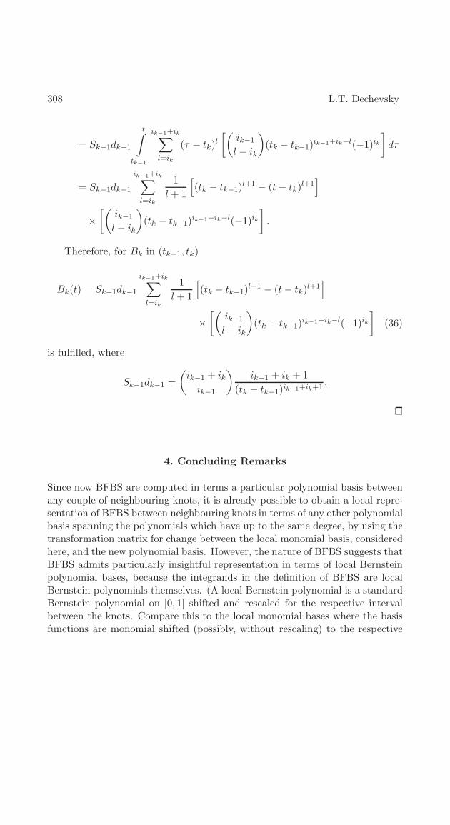
Therefore, for Bk in (tk−1, tk)


ik−1+ik∑

l=ik

1

l + 1

[

(tk − tk−1)l+1 − (t− tk)

l+1]

×

[(

ik−1

l − ik

)


]

(36)

is fulfilled, where

Sk−1dk−1 =

(

ik−1 + ik

ik−1

)

ik−1 + ik + 1

(tk − tk−1)ik−1+ik+1.

4. Concluding Remarks

Since now BFBS are computed in terms a particular polynomial basis betweenany couple of neighbouring knots, it is already possible to obtain a local repre-sentation of BFBS between neighbouring knots in terms of any other polynomialbasis spanning the polynomials which have up to the same degree, by using thetransformation matrix for change between the local monomial basis, consideredhere, and the new polynomial basis. However, the nature of BFBS suggests thatBFBS admits particularly insightful representation in terms of local Bernsteinpolynomial bases, because the integrands in the definition of BFBS are localBernstein polynomials themselves. (A local Bernstein polynomial is a standardBernstein polynomial on [0, 1] shifted and rescaled for the respective intervalbetween the knots. Compare this to the local monomial bases where the basisfunctions are monomial shifted (possibly, without rescaling) to the respective


knot.) This representation is closely related to the geometric-modelling prop-erties of the linear combinations of BFBS and will be studied in one of the twoother papers in the present sequence. On the other hand, for the purposes ofoperational calculus (which may be useful in the future as a toolbox in study-ing BFBS-based multiwavelet and other multilevel constructions), it may be ofinterest to represent BFBS in terms of the same polynomial basis uniformly inall intervals between neighbouring knots, i.e., globally. One natural choice ofsuch a basis is the monomial basis 1, t, t2, . . . tm, for an appropriate choiceof the degree m ∈ N. This topic will be addressed in the other one of the tworemaining papers in this sequence.

Acknowledgments

This work was partially supported by the 2005, 2006, 2007, 2008 and 2009Annual Research Grants of the R&D Group for Mathematical Modelling, Nu-merical Simulation and Computer Visualization at Narvik University College,Norway.

References

[1] L.T. Dechevsky. Expo-Rational B-Splines. Communication at the Fifth In-ternational Conference on Mathematical Methods for Curves and Surfaces,Tromsø’2004, Norway (unpublished).

[2] L.T. Dechevsky. Generalized Expo-Rational B-Splines. Communication atthe Seventh International Conference on Mathematical Methods for Curvesand Surfaces, Tønsbeg’2008, Norway (unpublished).

[3] L.T. Dechevsky, Beta-function B-splines: Definition and basic properties,Int. J. Pure Appl. Math., 65, No. 3 (2010), 279-295.

[4] L.T. Dechevsky, B. Bang, A. Laks̊a. Generalized Expo-Rational B-splines.Int. J. Pure Appl. Math., 57(1) (2009) 833–872.

[5] L.T. Dechevsky, A. Laks̊a, B. Bang. Expo-Rational B-splines. Int. J. PureAppl. Math., 27(3) (2006) 319–369.

[6] L.T. Dechevsky, A. Laks̊a, B. Bang. NUERBS form of expo-rational B-splines. Int. J. Pure Appl. Math. 32(1) (2006) 11–32.

310 L.T. Dechevsky

[7] L.T. Dechevsky, E. Quak, A. Laks̊a, A.R. Kristoffersen. Expo-rationalspline multiwavelets: a first overview of definitions, properties, general-izations and applications. In: F. Truchetet, O. Laligant (eds.) WaveletApplications in Industrial Processing V, Proceedings of SPIE, vol. 6763(2007), article 676308.

[8] A. Laks̊a. Basic Properties of Expo-rational B-splines and Practical Use inComputer Aided Geometric Design, Doctor Philos. Dissertation, Universityof Oslo, Norway, 2007.

[9] A. Laks̊a, B. Bang, L.T. Dechevsky. Exploring Expo-Rational B-splines forCurves and Surfces. In: Mathematical Methods for Curves and Surfaces, M.Dæhlen, K. Mørken, L. Schumaker (eds.), Nashboro Press, 2005, 253–262.

Documents

International Journal of Pure and Applied Mathematics ... · PDF fileInternational Journal of Pure and Applied Mathematics |||||{Volume 65 No. 3 2010, 297-310 EVALUATION OF BETA-FUNCTION