925

International Journal of Supply and Operations Management

IJSOM

November 2015, Volume 2, Issue 3, pp. 925-946

ISSN-Print: 2383-1359

ISSN-Online: 2383-2525

www.ijsom.com

A stochastic programming approach for a multi-site supply chain planning in

textile and apparel industry under demand uncertainty

Houssem Felfel

*a, Omar Ayadi

a and Faouzi Masmoudi

a

a National Engineering School of Sfax (ENIS), University of Sfax, Tunisia, Road Soukra,

Sfax, Tunisia

Abstract

In this study, a new stochastic model is proposed to deal with a multi-product, multi-period,

multi-stage, multi-site production and transportation supply chain planning problem under

demand uncertainty. A two-stage stochastic linear programming approach is used to maximize the

expected profit. Decisions such as the production amount, the inventory level of finished and

semi-finished product, the amount of backorder and the quantity of products to be transported

between upstream and downstream plants in each period are considered. The robustness of

production supply chain plan is then evaluated using statistical and risk measures. A case study

from a real textile and apparel industry is shown in order to compare the performances of the

proposed stochastic programming model and the deterministic model.

Keywords: multi-site; supply chain planning; stochastic programming; textile; robustness.

1. Introduction

Modern process industries operate no more as traditional single-plant but as multi-site supply

chain structure where different production facilities are serving a global market. In the last

decades, supply chain management has received a remarkable interest in order to cope with highly

* Corresponding author email address: houssem.felfel@gmail.com

Felfel, Ayadi and Dadgar

926

continuous competition. Supply chain planning is an important process within the supply chain

management involving decisions undertaken by a company from the procurement of raw materials

to the shipping of end products to the customer. The supply chain planning problem can be

classified following the time horizon into three categories: strategic, tactical, and operational

(Chopra and Meindl 2010). The strategic level concerns the design and the structure of the supply

chain over a long time horizon between five and ten years. The operational level is related to short

term decisions lasting from few days to few weeks such as scheduling, lot sizing and sequencing.

The tactical planning model is between these two extremes and includes procurement, production,

and distribution decisions.

This study is particularly motivated by a tactical supply chain planning problem faced by

multi-site supply network from textile and apparel industry. Textile manufacturing process

consists of knitting and dyeing, cutting, embroidery, cloth making, and packaging stages. Each

production stage may include more than one plant, forming a multi-site, multi-stage

manufacturing environment.

The fluctuation of products demand is among the most important sources of uncertainty in the

textile and apparel industry. In fact, the customer demand could be determined only at the end of

the planning horizon. The under-estimation of overall demand leads either to loss sales or

unsatisfied customers. However, the over-estimation of the products demand results in high

production and inventory costs.

In this paper, we deal with a multi-product, multi-period, multi-stage, multi-site supply chain

planning problem under customer demand uncertainty. A two-stage stochastic programming

model is developed in order to incorporate the effects of the uncertainty in the considered problem.

Decision variables such as amounts of production and quantity to be transported between different

manufacturing facilities are considered as first-stage variables and are assumed to be made before

the realization of the uncertainty. Otherwise, decision variables related to the inventory level,

backorder amount, and transportation amount of end products to be shipped to the customer are

considered as second-stage variables made after the realization of uncertain demand. Subsequently,

the robustness of production planning solution is evaluated. Statistical metric and financial risk

metric, such as value at risk (VaR) and conditional VaR (CVaR), are calculated in order to evaluate

the robustness of planning solutions generated by the stochastic programming model compared to

the deterministic model. Besides, a real example from a textile and apparel manufacturer case in

Tunisia is illustrated to compare the proposed stochastic model with the traditional deterministic

supply chain planning model.

The main scientific contribution of this work is to develop a new stochastic model for a

multi-product, multi-period, multi-stage, multi-site supply chain production and transportation

planning problem under customer demand uncertainty. Besides, the proposed model and the

evaluation approach are applied to a real case study from textile and apparel industry.

The rest of the paper is organized as follows. In the next section, we present the literature review

of related topics. Section 3 describes the textile and apparel supply network under consideration.

In section 4, a two-stage stochastic formulation is proposed in order to incorporate demand

Int J Supply Oper Manage (IJSOM)

927

uncertainty in the supply chain planning problem. Section 5 describes the stochastic programming

algorithm. By conducting a real case study, Section 6 verifies the effectiveness and the robustness

of the proposed stochastic model compared to the deterministic model. Finally, conclusions,

limitations of the developed model, and future research directions are drawn in Section 7.

2. Literature review

To cope with highly competitive and global markets, the structure of manufacturing companies

has changed from traditional single-site to multi-site structure. Multi-site production planning

problems have received a lot of attention in the literature.

Most of the papers dealing with multi-site production planning problem focus on deterministic

approaches. Toni and Meneghetti (2000) addressed the production planning problem of a

textile-apparel industry supply chain. The authors investigate the influence of production planning

period length as well as color assortment in the system's time performance. A real case study from

an Italian network of firms was treated using a simulation model. Lin and Chen (2007) developed

a monolithic model of a multi-stage multi-site multi-item production planning problem. The

proposed model combined simultaneously two different time scales, i.e., monthly and daily time

buckets. A practical example from the thin film transistor-liquid crystal display (TFT-LCD)

industry is illustrated to explain the planning model. Leung et al (2003) studied a multi-site

aggregate production planning problem of a multinational lingerie company located in Hong

Kong using a goal programming approach. Three major objective functions were considered,

which are minimization of the cost of workers hiring and laying-off, the maximization of profit

and the minimization of the over-or under-utilization of import quotas of different products. Shah

and Ierapetritou (2012) treated the integrated planning and scheduling problem for multi-site,

multi-product batch plants using the augmented Lagrangian decomposition method. Given the

fixed demand forecast, the model aims to minimize production, storage, shipping, and backorder

costs. Felfel et al (2014) proposed a multi-objective, multi-stage, multi-product, and multi-period

model for production and transportation planning in a multi-site manufacturing network. The

developed model aims simultaneously to minimize the total cost and to maximize products’

quality level. It should be noted that most of the papers dealing with multi-site production

planning problem focus on deterministic solution. However, real production planning problems

are characterized by several sources of uncertainty. Hence, the assumption that all model

parameters are known with certainty will lead to non-optimal and even unrealistic results.

Many approaches have been proposed in the literature to cope with uncertainty. According to

Sahinidis (2004), these approaches can be classified into four major categories: fuzzy

programming approach, robust optimization approach, stochastic programming approach, and

stochastic dynamic programming approach. Stochastic programming approach (Birge and

Louveaux, 1997; Dantzig, 1955) is one of the most widely spread techniques in the literature used

in supply chain planning problem under uncertainty. In this approach, the decision variables of the

optimization problem are divided into two sets. The decision variables of the first stage called

“here and now” decisions have to be made before the realization of uncertainty. Subsequently, the

second-stage decision variables are chosen after the presence of uncertain parameters in order to

Felfel, Ayadi and Dadgar

928

correct the infeasibilities caused by uncertainty realization (“wait and see” decisions). Therefore,

the value of the objective function is the sum of first-stage decision variables and the second-stage

expected recourse variables.

Several works in the literature have been interested in stochastic programming model for supply

chain planning problem.

Gupta and Maranas (2000) proposed a multi-site midterm supply-chain planning problem under

demand uncertainty using two-stage stochastic programming approach. The supply chain

decisions are devised into two categories: manufacturing decisions and logistics decisions. The

manufacturing decisions are taken “here and now” before the realization of uncertainty while the

logistics decisions are postponed in a “wait and see” mode. A single period is considered in the

developed model.

Leung et al (2006) developed a two-stage stochastic programming model in order to optimize a

multi-site aggregate medium-term production planning problem under an uncertain environment.

The first-stage decisions include the amount of manufactured product in regular-time and

overtime, volume of subcontracted products and number of required workers, hired workers and

laid-off workers. Decisions such as inventory level of products, and the amount of

under-fulfilment products are considered as second-stage decisions. The effectiveness of the

proposed model was highlighted through a real-world case study from a multinational lingerie

company situated in Hong Kong. Karabuk (2008) considered a yarn production planning problem

under demand uncertainty in a textile manufacturing supply chain. The author developed a

stochastic programming model where the rover configuration, frame configuration, and

production quantity are the first-stage decisions. Inventory level is considered as recourse decision.

A two-step preprocessing algorithm is developed to solve the optimization problem and to reduce

computational complexities of the large-scale resulting model. Nevertheless, these works didn’t

consider transportation in the mathematical optimization model.

Nagar and Jain (2008) studied a multi-period supply chain planning problem for new product

launches under demand uncertainty. A two-stage stochastic programming approach is developed

in order to incorporate uncertainty. Production quantity, raw material procurement, and capacity

utilization are presented as “here and now” decisions. Outsourcing, inventory and shipping of end

product to customer are proposed as “wait and see” decisions until the realization of uncertain

demand. Subsequently, this model is extended using a multi-stage stochastic programming

formulation. Mirzapour Al-e-hashem et al (2011a) proposed a mid-term multi-product,

multi-period, multi-site production-distribution planning problem under cost and demand

uncertainties. A two-stage stochastic programming model was developed to incorporate the

uncertain parameters. Mirzapour Al-e-Hashem et al (2011b) developed a multi-site, multi-product,

multi-period aggregate production planning problem. To solve this problem, a new robust

multi-objective mixed integer nonlinear programming model was proposed. The common critic of

these works is the consideration of a single production stage in the planning problem.

Awudu and Zhang (2013) developed a two-stage stochastic programming model for a production

planning problem in a biofuel supply chain under uncertainty in order to maximize the expected

Int J Supply Oper Manage (IJSOM)

929

profit. Amount of products to be produced, and amount of raw materials to be purchased and

consumed are considered as the first-stage decisions. Decisions such as backlog, lost sales, and

sold products quantity are considered as second-stage decisions. A case study from a biofuel

supply chain is illustrated to demonstrate the effectiveness of the proposed model. A single period

and a single production stage are taken into account in this work.

In the context of supply chain planning, robustness can be defined as a measure of resilience of

the objective function, usually cost or profit, to change under random events and uncertain

parameters. Therefore, the evaluation of robustness represents an important issue in order to

assess the performance of the supply chain planning in the face of parameter uncertainty. Vin and

Ierapetritou (2001) developed a strategy to quantify scheduling robustness in the face of

uncertainty under uncertainty. To do so, several robustness metrics were used, such as the

corrected standard deviation, the deterministic standard deviation and the extent of violation. Lin

et al (2011) proposed a stochastic programming model for strategic capacity planning in thin film

transistor-liquid crystal display industry. The robustness of the capacity plan is evaluated using

financial risk measures, such as the value at risk and the conditional value at risk. Although the

evaluation of robustness was performed in scheduling and strategic planning, this concept was not

extended to tactical multi-site supply chain production and transportation planning problem.

3. Problem statement

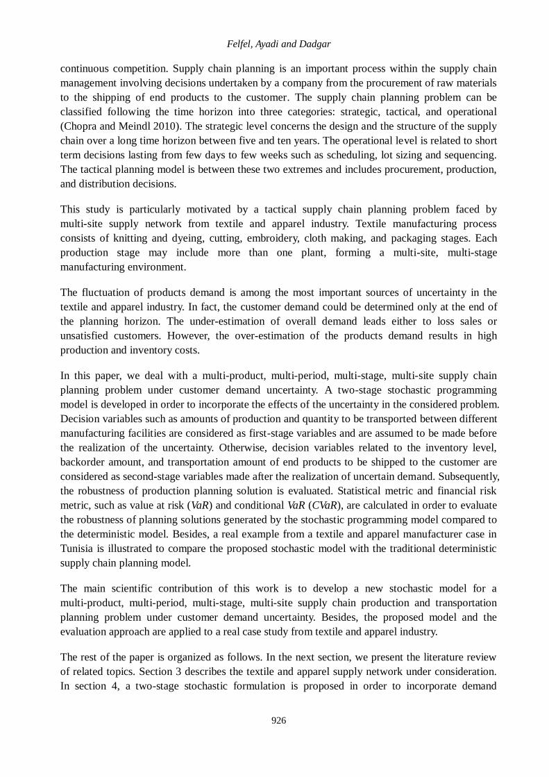
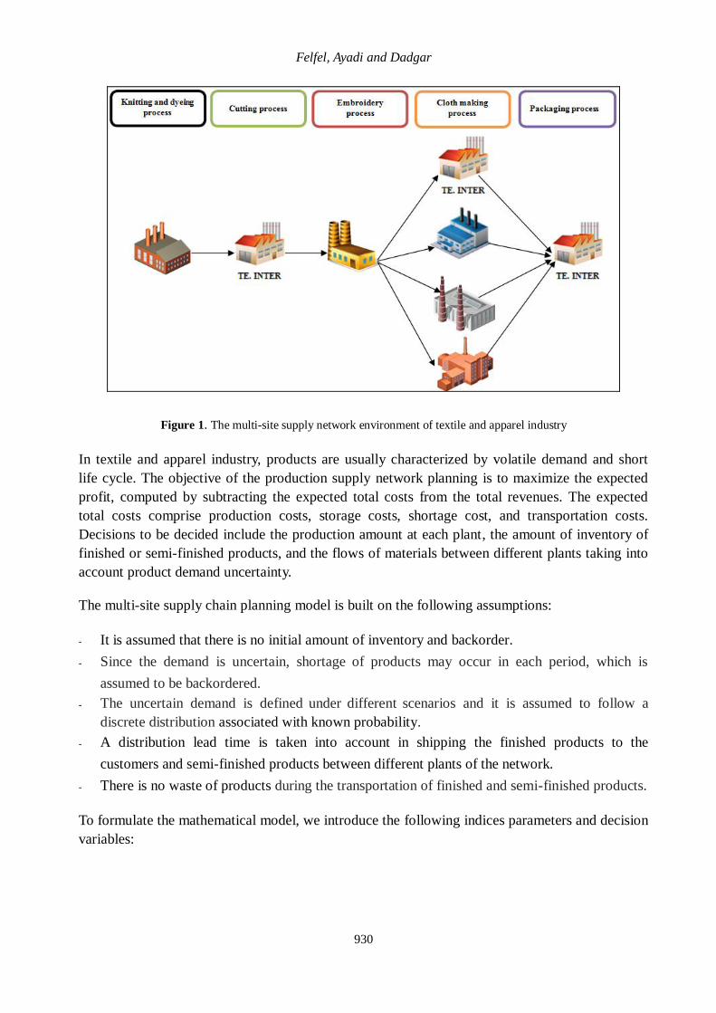
In this paper, we considered a supply network from the textile and apparel industry wherein the

finished product is processed by means of different production stages. The textile and apparel

manufacturing process consists of five main stages: knitting and dyeing, cutting, embroidery,

cloth making, and packaging. Each production stage may include more than one plant establishing

a multi-site supply network manufacturing environment as illustrated in Figure 1. The considered

supply network is composed of an internal plant (Textile-International “TE-INTER”) and four

subcontractors: a dyer and a knitter, an embroiderer, and three cloth makers. The TE-INTER

company is formed of three manufacturing departments which are cutting, packaging, and cloth

making. Other activities such as knitting, dyeing, and embroidery are subcontracted because of the

lack of technical competence and resources. Cloth making operation can be also subcontracted in

order to extend the production capacity and to fulfill all the customer demand.

Felfel, Ayadi and Dadgar

930

Figure 1. The multi-site supply network environment of textile and apparel industry

In textile and apparel industry, products are usually characterized by volatile demand and short

life cycle. The objective of the production supply network planning is to maximize the expected

profit, computed by subtracting the expected total costs from the total revenues. The expected

total costs comprise production costs, storage costs, shortage cost, and transportation costs.

Decisions to be decided include the production amount at each plant, the amount of inventory of

finished or semi-finished products, and the flows of materials between different plants taking into

account product demand uncertainty.

The multi-site supply chain planning model is built on the following assumptions:

- It is assumed that there is no initial amount of inventory and backorder.

- Since the demand is uncertain, shortage of products may occur in each period, which is

assumed to be backordered.

- The uncertain demand is defined under different scenarios and it is assumed to follow a

discrete distribution associated with known probability.

- A distribution lead time is taken into account in shipping the finished products to the

customers and semi-finished products between different plants of the network.

- There is no waste of products during the transportation of finished and semi-finished products.

To formulate the mathematical model, we introduce the following indices parameters and decision

variables:

Int J Supply Oper Manage (IJSOM)

931

Indices

iL Set of direct successor plant of i.

jST Set of stages (j= 1,2, ..., N).

i, i’ Production plant index (i,i’ = 1, 2 , ...,I) where i belongs to stage n and i’

belongs to stage n+1.

k Product index (k = 1,2, ..., K).

t Period index (t = 1,2, ..., T).

s Scenario index (s = 1,2,. . .,S).

Decision variables

iktP Production amounts of product k at plant i in period t in regular-time.

s

iktS Amounts of end of period inventory of product k for scenario s at plant i

in period t.

s

iktJS Amounts of end of period inventory of semi-finished product k for

scenario s at plant i in period t.

s

ktBD Backorder amounts of finished product k for scenario s in period t.

',i i ktTR Amounts of product k transported from plant i to i’ in period t.

,

s

i CUS ktTR Amounts of product k transported from the last plant i to customer for

scenario s in period t.

,i kQ Amounts of product k received by plant i for scenario s in period t.

Parameters

ikcp Unit cost of production for product k in regular-time at plant i.

',i i kct Unit cost of transportation between plant i and i’ of production for

product k.

,i CUS kct Unit cost of transportation between the last plant i and the customer.

ikcs Unit cost of inventory of finished or semi-finished product k at plant i.

kcb Unit cost of backorder of product k.

kpr Unit sales price of finished product k.

Felfel, Ayadi and Dadgar

932

itcapp Production capacity at plant i in normal working hours in period t.

itcaps Storage capacity at plant i in period t.

',i i tcaptr Transportation capacity at plant i in period t.

s

ktD Demand of finished product k for scenario s in period t.

kb Time needed for the production of a product entity k [min].

DL Delivery time of the transported quantity.

s The occurrence probability of scenario s where 1

1S

s

s

4. Proposed two-stage stochastic programming model

Due to the uncertainty of finished products demand, the deterministic model is inappropriate to

optimize the expected net profit. Therefore, a two-stage stochastic programming model is

proposed in order to incorporate uncertainty in the decision-making. It should be noted that the

stages of the stochastic programing model correspond to different steps of decision-making and it

is not related to time periods. Due to the considerable lead times required in the production

process, the production amounts in each plant and the product amounts to be transported between

upstream and downstream plants are taken “here and now” before the realization of the

uncertainty. Other decision variables such as inventory, backorder size and flow of finished

products to be shipped to the customer can be achieved in a “wait and see” mode.

Consequently, the two-stage stochastic programming model can be formulated as follows. The

objective function (1) aims to maximize the expected profit obtained by subtracting the total

expected cost from the expected revenue. The occurrence probability of each scenario is

considered in order to calculate the expected revenue and the expected cost. The total cost

includes production cost, inventory cost, backorder cost, transportation cost of semi-products

between upstream and downstream plants, and transportation cost of finished products to

customer.

Constraint (2) is the balance for the inventory level of products in each production stage excluding

the last stage.

,

1 1 1 1

, , , ', ',

1 1 1

[ ] ( )S T K I

s s s s

k i CUS kt ik ikt ikt

s t k i

T K Is s

i CUS k i CUS kt k k t ik ikt i i k i i kt

t k i

Max E Profit pr TR cs S JS

ct TR cb BD cp P ct TR

(1)

Int J Supply Oper Manage (IJSOM)

933

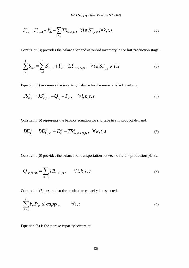
Constraint (3) provides the balance for end of period inventory in the last production stage.

Equation (4) represents the inventory balance for the semi-finished products.

Constraint (5) represents the balance equation for shortage in end product demand.

Constraint (6) provides the balance for transportation between different production plants.

Constraints (7) ensure that the production capacity is respected.

Equation (8) is the storage capacity constraint.

, , 1 ',

'

, , , ,i

s s

ik t ik t ikt i i kt j N

i L

S S P TR i ST k t s

(2)

, , 1 ,

1 1

, , , ,j N

I Is s s

ik t ik t ikt i CUS kt

i i

S S P TR i ST k t s

(3)

, , 1 , , , ,ikt

s s

ik t ik t iktJS JS Q P i k t s (4)

, 1 , , , ,s s s s

kt k t kt i CUS ktBD BD D TR k t s

(5)

' , ',

'

, , , ,i

i k t DL i i kt

i L

Q TR i k t s

(6)

1

, ,K

k ikt it

k

b P capp i t

(7)

Felfel, Ayadi and Dadgar

934

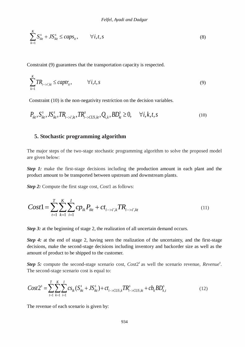
Constraint (9) guarantees that the transportation capacity is respected.

5. Stochastic programming algorithm

The major steps of the two-stage stochastic programming algorithm to solve the proposed model

are given below:

Step 1: make the first-stage decisions including the production amount in each plant and the

product amount to be transported between upstream and downstream plants.

Step 2: Compute the first stage cost, Cost1 as follows:

', ',

1 1 1

1T K I

ik ikt i i k i i kt

t k i

Cost cp P ct TR

(11)

Step 3: at the beginning of stage 2, the realization of all uncertain demand occurs.

Step 4: at the end of stage 2, having seen the realization of the uncertainty, and the first-stage

decisions, make the second-stage decisions including inventory and backorder size as well as the

amount of product to be shipped to the customer.

Step 5: compute the second-stage scenario cost, Cost2s as well the scenario revenue, Revenue

s.

The second-stage scenario cost is equal to:

, , ,

1 1 1

2 ( )T K I

s s s s s

ik ikt ikt i CUS k i CUS kt k k t

t k i

Cost cs S JS ct TR cb BD

(12)

The revenue of each scenario is given by:

1

, , ,K

s s

ikt ikt it

k

S JS caps i t s

(8)

',

1

, , ,K

i i kt it

k

TR captr i t s

(9)

Constraint (10) is the non-negativity restriction on the decision variables.

', , ,, , , , , , 0, , , ,s s s s

ikt ikt ikt i i kt i CUS kt i k ktP S JS TR TR Q BD i k t s

(10)

Int J Supply Oper Manage (IJSOM)

935

,

1 1 1

T K Is s

k i CUS kt

t k i

Revenue pr TR

(13)

Step 6: Calculate the expected total profit E[Profit] as follows:

1

[ ] ( 2 ) 1S

s s s

s

E Profit Revenue Cost Cost

(14)

The proposed two-stage programming model is solved using the stochastic programming solver

for multistage stochastic programs with recourse of Lingo 14.0 software.

6. Computational experiments

The main purpose of this section is to evaluate the effectiveness and the robustness of stochastic

model in comparison with the deterministic model using real case industrial data from textile and

apparel industry. In Section 6.1, the related input data are described. Then, the deterministic and

stochastic models are solved and the quality of the obtained solutions is compared using stochastic

programming parameters in Section 6.2. It is worthwhile mentioning that the deterministic model

is widely used in the literature (Kall and Wallace, 1994; Birge and Louveaus, 1997; Awudu and

Zhang, 2013) to evaluate the performance of the stochastic programming model. To solve the

deterministic model, the random parameters are assumed to be known with certainty and thus only

one scenario with mean random values is considered.

Giving the simulation results, we evaluate the robustness of the proposed model through many

statistical and risk metrics as detailed in Section 6.3. Section 6.4 gives other case studies under

randomly generated customer demand to validate the obtained results. The experiments are

conducted using LINGO 14.0 package program and MS-Excel 2010 with an INTEL(R) Core (TM)

and 2 GB RAM.

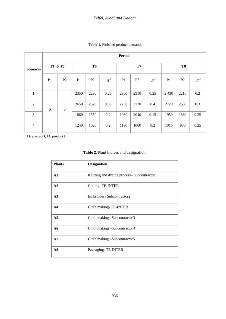
6.1. Industrial case description

In this section, real data is provided from a medium and small enterprise located in Tunisia in

textile and apparel industry. The planning horizon of the planning problem covers two months and

the length of a period is one week. On the basis of past sales records and future long-term and

short-term contracts, the future economy can be assumed to be one of four scenarios: poor, fair,

good, or boom. The market demand of the finished product P1 and P2 under each scenario is

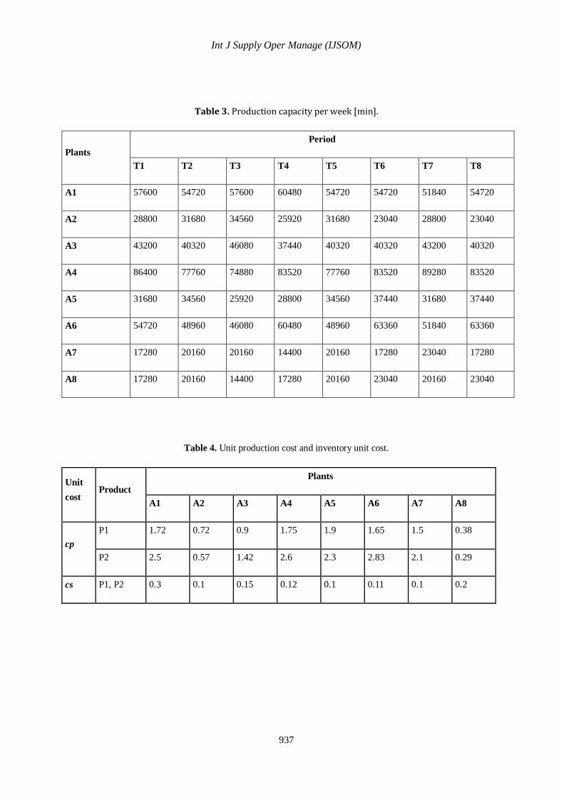
reported in Table1. Different plant indices are listed in Table 2. Table 3 described the production

capacities of different plants. It should be noted that the production capacity varies from one

period to another because of the absenteeism. Table 4 provides information about production and

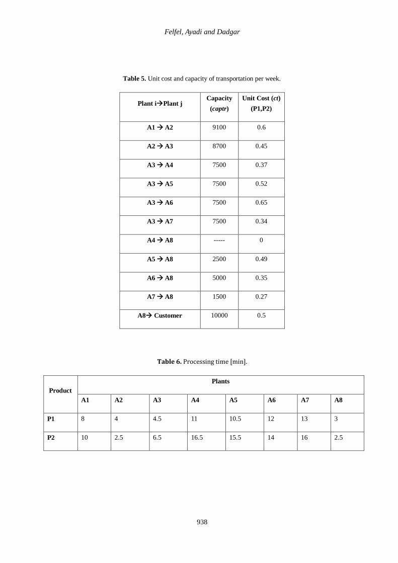
inventory unit cost. The transportation unit cost and capacity are shown in Table 5. The processing

times of different manufacturing process are reported in Table 6.

Felfel, Ayadi and Dadgar

936

Table 1. Finished product demand.

Scenario

Period

T1 T5 T6 T7 T8

P1 P2 P1 P2 s P1 P2

s P1 P2 s

1

0 0

2350 2230 0.25 2300 2310 0.25 2 430 2210 0.2

2 2650 2520 0.35 2730 2770 0.4 2720 2530 0.3

3 1860 1550 0.2 1930 2040 0.15 1950 1860 0.25

4 1240 1020 0.2 1180 1060 0.2 1010 930 0.25

P1: product 1, P2: product 2.

Table 2. Plant indices and designation.

Plants Designation

A1 Knitting and dyeing process– Subcontractor1

A2 Cutting- TE-INTER

A3 Embroidery Subcontractor2

A4 Cloth making- TE-INTER

A5 Cloth making –Subcontractor3

A6 Cloth making –Subcontractor4

A7 Cloth making –Subcontractor5

A8 Packaging- TE-INTER

Int J Supply Oper Manage (IJSOM)

937

Table 3. Production capacity per week [min].

Plants

Period

T1 T2 T3 T4 T5 T6 T7 T8

A1 57600 54720 57600 60480 54720 54720 51840 54720

A2 28800 31680 34560 25920 31680 23040 28800 23040

A3 43200 40320 46080 37440 40320 40320 43200 40320

A4 86400 77760 74880 83520 77760 83520 89280 83520

A5 31680 34560 25920 28800 34560 37440 31680 37440

A6 54720 48960 46080 60480 48960 63360 51840 63360

A7 17280 20160 20160 14400 20160 17280 23040 17280

A8 17280 20160 14400 17280 20160 23040 20160 23040

Table 4. Unit production cost and inventory unit cost.

Unit

cost Product

Plants

A1 A2 A3 A4 A5 A6 A7 A8

cp

P1 1.72 0.72 0.9 1.75 1.9 1.65 1.5 0.38

P2 2.5 0.57 1.42 2.6 2.3 2.83 2.1 0.29

cs P1, P2 0.3 0.1 0.15 0.12 0.1 0.11 0.1 0.2

Felfel, Ayadi and Dadgar

938

Table 5. Unit cost and capacity of transportation per week.

Plant iPlant j Capacity

(captr)

Unit Cost (ct)

(P1,P2)

A1 A2 9100 0.6

A2 A3 8700 0.45

A3 A4 7500 0.37

A3 A5 7500 0.52

A3 A6 7500 0.65

A3 A7 7500 0.34

A4 A8 ----- 0

A5 A8 2500 0.49

A6 A8 5000 0.35

A7 A8 1500 0.27

A8 Customer 10000 0.5

Table 6. Processing time [min].

Product

Plants

A1 A2 A3 A4 A5 A6 A7 A8

P1 8 4 4.5 11 10.5 12 13 3

P2 10 2.5 6.5 16.5 15.5 14 16 2.5

Int J Supply Oper Manage (IJSOM)

939

6.2. Computational results

In order to evaluate the impact of uncertainty parameters on the planning decisions, two stochastic

well-known measures were used: the expected value of perfect information (EVPI) and the value

of stochastic solution (VSS) (Birge and Louveaus 1997). The EVPI parameter helps to determine

the expected profit loss under uncertainty. It can be calculated as:

EVPI= WS –TSP (15)

Where TSP is the objective value of two-stage stochastic programming model and WS represents

the objective value of the “wait and see” model. The WS model involves a family of linear

programming models. Each model is associated with an individual scenario. The solution of the

WS model is obtained by weighting each individual scenario with its corresponding probability.

Such a model would allow to always make the best decision regardless of the uncertain

parameters which is not possible in practice.

The VSS parameter calculates the possible profit from solving the two-stage stochastic programing

model over the deterministic model. If the VSS is positive, it implies that the solutions of

stochastic programming model are better than those of the deterministic model. It is defined as:

VSS= TSP- EEV (16)

Where EEV represents the expected solution of deterministic model.

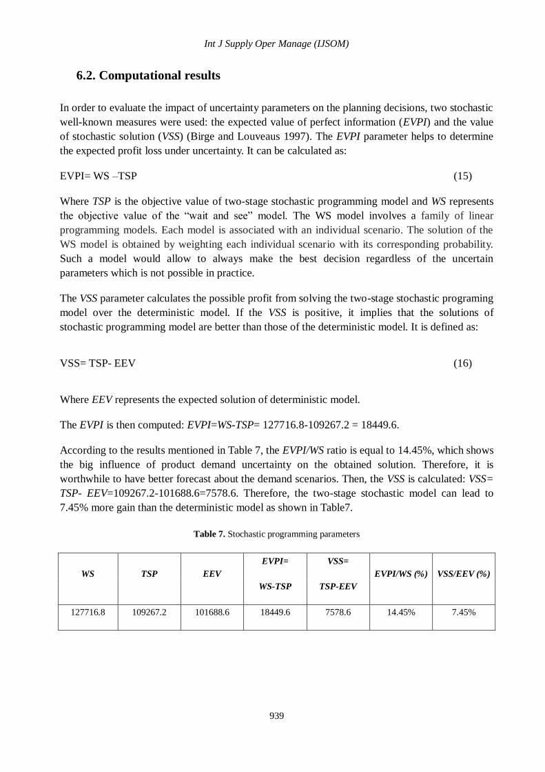
The EVPI is then computed: EVPI=WS-TSP= 127716.8-109267.2 = 18449.6.

According to the results mentioned in Table 7, the EVPI/WS ratio is equal to 14.45%, which shows

the big influence of product demand uncertainty on the obtained solution. Therefore, it is

worthwhile to have better forecast about the demand scenarios. Then, the VSS is calculated: VSS=

TSP- EEV=109267.2-101688.6=7578.6. Therefore, the two-stage stochastic model can lead to

7.45% more gain than the deterministic model as shown in Table7.

Table 7. Stochastic programming parameters

WS TSP EEV

EVPI=

WS-TSP

VSS=

TSP-EEV

EVPI/WS (%) VSS/EEV (%)

127716.8 109267.2 101688.6 18449.6 7578.6 14.45% 7.45%

Felfel, Ayadi and Dadgar

940

6.3. Robustness evaluation

6.3.1. Robustness evaluation metrics

In order to evaluate the robustness of the production planning, different statistical and risk metrics

were used. These metrics are basically:

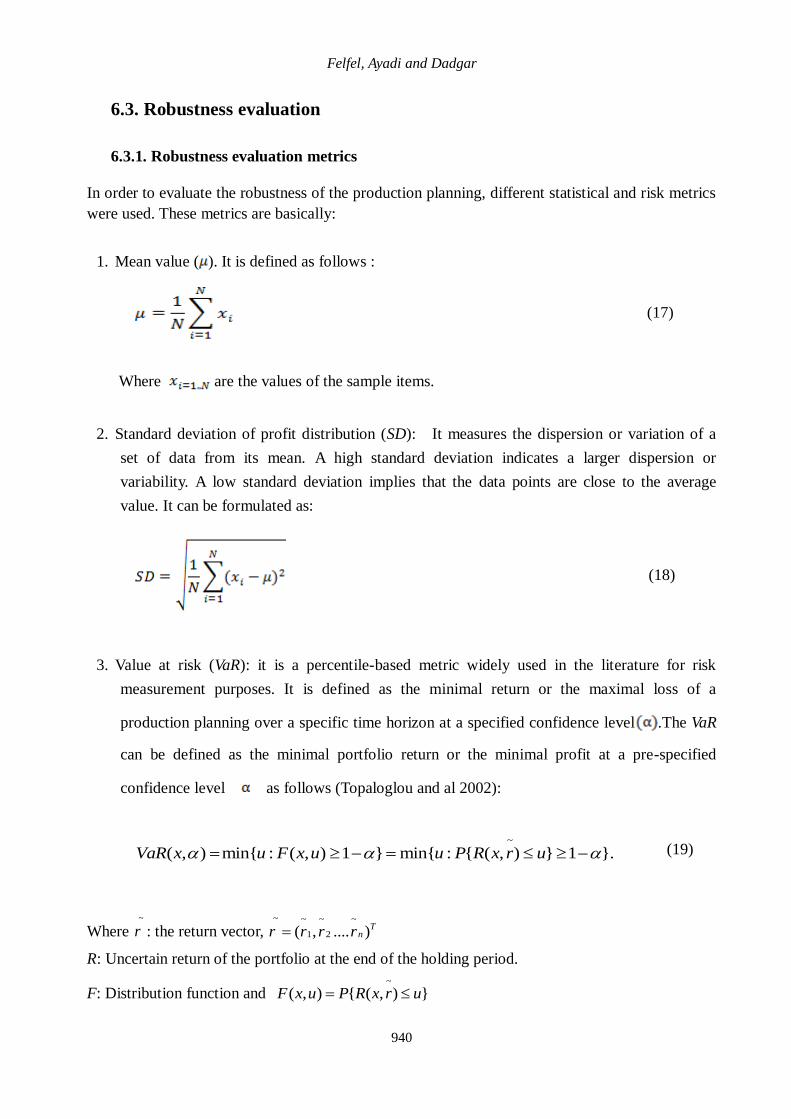
1. Mean value ( ). It is defined as follows :

(17)

Where are the values of the sample items.

2. Standard deviation of profit distribution (SD): It measures the dispersion or variation of a

set of data from its mean. A high standard deviation indicates a larger dispersion or

variability. A low standard deviation implies that the data points are close to the average

value. It can be formulated as:

(18)

3. Value at risk (VaR): it is a percentile-based metric widely used in the literature for risk

measurement purposes. It is defined as the minimal return or the maximal loss of a

production planning over a specific time horizon at a specified confidence level .The VaR

can be defined as the minimal portfolio return or the minimal profit at a pre-specified

confidence level as follows (Topaloglou and al 2002):

~

( , ) min{ : ( , ) 1 } min{ : { ( , ) } 1 }.VaR x u F x u u P R x r u (19)

Where~

r : the return vector,~ ~ ~ ~

1 2( , .... )Tnr r r r

R: Uncertain return of the portfolio at the end of the holding period.

F: Distribution function and ~

( , ) { ( , ) }F x u P R x r u

Int J Supply Oper Manage (IJSOM)

941

4. Conditional value at risk (CVaR): It is also called the mean shortfall, the mean excess loss,

and tail VaR. It is a more consistent and coherent measure of risk than the VaR since it gives

information about the average loss which exceeds the VaR. Topaloglou et al (2002) have

introduced a general definition of the CVaR for continuous and discrete distributions as

follows:

{ | ( , ) }

{ | ( , ) }

1( , ) (1 ) ( , )

1 1

s

s

s

s R x r z

s s

s R x r z

p

CVaR x z p R x r

(20)

Where ( , )z VaR x ;

ps Associated probability to the return value~ ~ ~ ~

1 2( , .... )Ts s s nsr r r r under a scenario s.

Both VaR and CVaR are calculated for different risk level (⍺): 0.85, 0.9, and 0.95.

6.3.2. Measurement of robustness

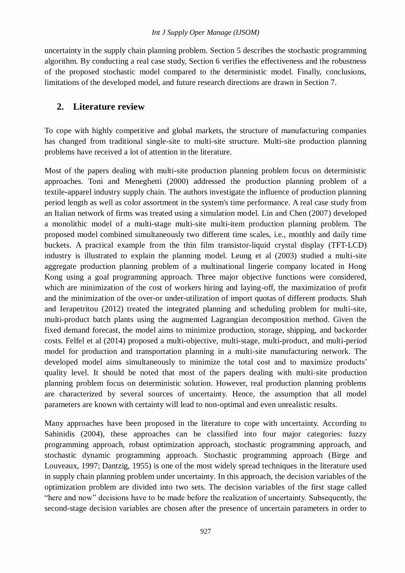
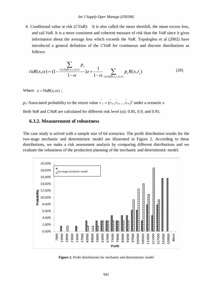
The case study is solved with a sample size of 64 scenarios. The profit distribution results for the

two-stage stochastic and deterministic model are illustrated in Figure 2. According to these

distributions, we make a risk assessment analysis by comparing different distributions and we

evaluate the robustness of the production planning of the stochastic and deterministic model.

Figure 2. Profit distributions for stochastic and deterministic model

Two-stage stochastic model

Deterministic model

Felfel, Ayadi and Dadgar

942

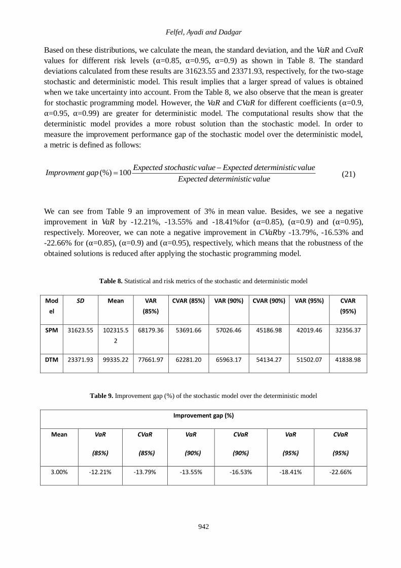
Based on these distributions, we calculate the mean, the standard deviation, and the VaR and CvaR

values for different risk levels (⍺=0.85, ⍺=0.95, ⍺=0.9) as shown in Table 8. The standard

deviations calculated from these results are 31623.55 and 23371.93, respectively, for the two-stage

stochastic and deterministic model. This result implies that a larger spread of values is obtained

when we take uncertainty into account. From the Table 8, we also observe that the mean is greater

for stochastic programming model. However, the VaR and CVaR for different coefficients (⍺=0.9,

⍺=0.95, ⍺=0.99) are greater for deterministic model. The computational results show that the

deterministic model provides a more robust solution than the stochastic model. In order to

measure the improvement performance gap of the stochastic model over the deterministic model,

a metric is defined as follows:

(%) 100Expected stochasticvalue Expected deterministicvalue

Improvment gapExpected deterministicvalue

(21)

We can see from Table 9 an improvement of 3% in mean value. Besides, we see a negative

improvement in VaR by -12.21%, -13.55% and -18.41%for (⍺=0.85), (⍺=0.9) and (⍺=0.95),

respectively. Moreover, we can note a negative improvement in CVaRby -13.79%, -16.53% and

-22.66% for (⍺=0.85), (⍺=0.9) and (⍺=0.95), respectively, which means that the robustness of the

obtained solutions is reduced after applying the stochastic programming model.

Table 8. Statistical and risk metrics of the stochastic and deterministic model

Mod

el

SD Mean VAR

(85%)

CVAR (85%) VAR (90%) CVAR (90%) VAR (95%) CVAR

(95%)

SPM 31623.55 102315.5

2

68179.36 53691.66 57026.46 45186.98 42019.46 32356.37

DTM 23371.93 99335.22 77661.97 62281.20 65963.17 54134.27 51502.07 41838.98

Table 9. Improvement gap (%) of the stochastic model over the deterministic model

Improvement gap (%)

Mean VaR

(85%)

CVaR

(85%)

VaR

(90%)

CVaR

(90%)

VaR

(95%)

CVaR

(95%)

3.00% -12.21% -13.79% -13.55% -16.53% -18.41% -22.66%

Int J Supply Oper Manage (IJSOM)

943

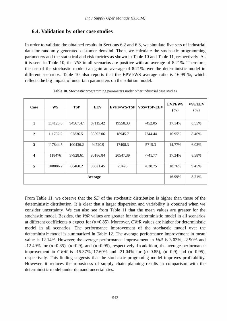
6.4. Validation by other case studies

In order to validate the obtained results in Sections 6.2 and 6.3, we simulate five sets of industrial

data for randomly generated customer demand. Then, we calculate the stochastic programming

parameters and the statistical and risk metrics as shown in Table 10 and Table 11, respectively. As

it is seen in Table 10, the VSS in all scenarios are positive with an average of 8.21%. Therefore,

the use of the stochastic model can gain an average of 8.21% over the deterministic model in

different scenarios. Table 10 also reports that the EPVI/WS average ratio is 16.99 %, which

reflects the big impact of uncertain parameters on the solution model.

Table 10. Stochastic programming parameters under other industrial case studies.

Case WS TSP EEV EVPI=WS-TSP VSS=TSP-EEV EVPI/WS

(%)

VSS/EEV

(%)

1 114125.8 94567.47 87115.42 19558.33 7452.05 17.14% 8.55%

2 111782.2 92836.5 85592.06 18945.7 7244.44 16.95% 8.46%

3 117844.5 100436.2 94720.9 17408.3 5715.3 14.77% 6.03%

4 118476 97928.61 90186.84 20547.39 7741.77 17.34% 8.58%

5 108886.2 88460.2 80821.45 20426 7638.75 18.76% 9.45%

Average 16.99% 8.21%

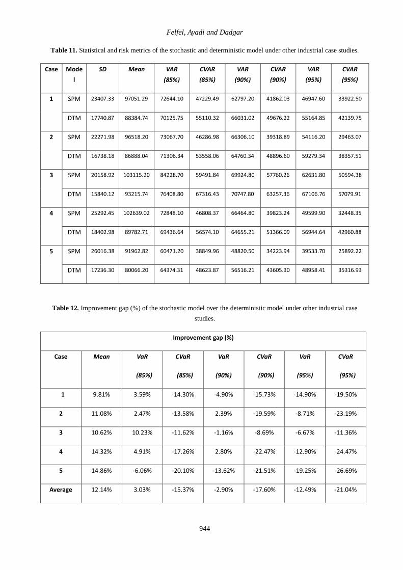
From Table 11, we observe that the SD of the stochastic distribution is higher than those of the

deterministic distribution. It is clear that a larger dispersion and variability is obtained when we

consider uncertainty. We can also see from Table 11 that the mean values are greater for the

stochastic model. Besides, the VaR values are greater for the deterministic model in all scenarios

at different coefficients ⍺ expect for (⍺=0.85). Moreover, CVaR values are higher for deterministic

model in all scenarios. The performance improvement of the stochastic model over the

deterministic model is summarized in Table 12. The average performance improvement in mean

value is 12.14%. However, the average performance improvement in VaR is 3.03%, -2.90% and

-12.49% for (⍺=0.85), (⍺=0.9), and (⍺=0.95), respectively. In addition, the average performance

improvement in CVaR is -15.37%,-17.60% and -21.04% for (⍺=0.85), (⍺=0.9) and (⍺=0.95),

respectively. This finding suggests that the stochastic programing model improves profitability.

However, it reduces the robustness of supply chain planning results in comparison with the

deterministic model under demand uncertainties.

Felfel, Ayadi and Dadgar

944

Table 11. Statistical and risk metrics of the stochastic and deterministic model under other industrial case studies.

Case Mode

l

SD Mean VAR

(85%)

CVAR

(85%)

VAR

(90%)

CVAR

(90%)

VAR

(95%)

CVAR

(95%)

1 SPM 23407.33 97051.29 72644.10 47229.49 62797.20 41862.03 46947.60 33922.50

DTM 17740.87 88384.74 70125.75 55110.32 66031.02 49676.22 55164.85 42139.75

2 SPM 22271.98 96518.20 73067.70 46286.98 66306.10 39318.89 54116.20 29463.07

DTM 16738.18 86888.04 71306.34 53558.06 64760.34 48896.60 59279.34 38357.51

3 SPM 20158.92 103115.20 84228.70 59491.84 69924.80 57760.26 62631.80 50594.38

DTM 15840.12 93215.74 76408.80 67316.43 70747.80 63257.36 67106.76 57079.91

4 SPM 25292.45 102639.02 72848.10 46808.37 66464.80 39823.24 49599.90 32448.35

DTM 18402.98 89782.71 69436.64 56574.10 64655.21 51366.09 56944.64 42960.88

5 SPM 26016.38 91962.82 60471.20 38849.96 48820.50 34223.94 39533.70 25892.22

DTM 17236.30 80066.20 64374.31 48623.87 56516.21 43605.30 48958.41 35316.93

Table 12. Improvement gap (%) of the stochastic model over the deterministic model under other industrial case

studies.

Improvement gap (%)

Case Mean VaR

(85%)

CVaR

(85%)

VaR

(90%)

CVaR

(90%)

VaR

(95%)

CVaR

(95%)

1 9.81% 3.59% -14.30% -4.90% -15.73% -14.90% -19.50%

2 11.08% 2.47% -13.58% 2.39% -19.59% -8.71% -23.19%

3 10.62% 10.23% -11.62% -1.16% -8.69% -6.67% -11.36%

4 14.32% 4.91% -17.26% 2.80% -22.47% -12.90% -24.47%

5 14.86% -6.06% -20.10% -13.62% -21.51% -19.25% -26.69%

Average 12.14% 3.03% -15.37% -2.90% -17.60% -12.49% -21.04%

Int J Supply Oper Manage (IJSOM)

945

7. Conclusion

In this paper, we propose a multi-product, multi-period, multi-stage, multi-site production and

transportation supply chain planning problem faced by textile and apparel industry under demand

uncertainty. In order to incorporate the effects of the uncertainty in the supply chain planning

problem, a two-stage stochastic model is developed. A real case study from a textile and apparel

supply network is illustrated to verify the effectiveness and the robustness of the developed model.

According to the computational results, the proposed stochastic programming model provides s

higher expected profit and profit mean value than the deterministic model under demand

uncertainty. However, the proposed stochastic model leads to less robust solutions in comparison

with the deterministic model. Improving the robustness of the planning solutions in the face of

uncertainty represents an interesting future work. This perspective can be addressed by means of

risk management models that incorporate risk measures into the stochastic programming model.

Acknowledgements

This research and innovation is carried out in the context of a thesis MOBIDOC funded by the

European Union under the program PASRI. The authors are grateful to LINDO Systems Inc for

providing us with a free educational research license of the extended version of LINGO 14.0

software package.

References

Awudu, I., & Zhang, J. (2013).Stochastic production planning for a biofuel supply chain under

demand and price uncertainties. Applied Energy, 103, 189-19.

Birge, J. R., & Louveaux, F. (1997). Introduction to Stochastic Programming. New York:

Springer.

Chopra, S., & Meindl, P. (2010). Supply chain management: Strategy, planning, and

operation(4th ed.). Pearson Education, Inc : Upper Saddle River, New Jersey.

Dantzig, G. B. (1955). Linear programming under uncertainty. Management Science 1, 197.

Felfel, H., Ayadi, O., & Masmoudi, F. (2014). Multi-objective Optimization of a Multi-site

Manufacturing Network. Lecture Notes in Mechanical Engineering, 69-76.

Gupta, A., & Maranas, C. D. (2000). A Two-Stage Modeling and Solution Framework for Multisite

Midterm Planning under Demand Uncertainty. Industrial & Engineering Chemistry Research, 39,

3799-3813.

Lin J.T., & Chen Y.Y. (2007). A Multi-site Supply Network Planning Problem Considering

Variable Time Buckets - A TFT-LCD Industry Case. International Journal of Advanced

Manufacturing Technology,33(9-10), 1031-1044.

Felfel, Ayadi and Dadgar

946

Kall, P. & Wallace, S.W. (1994). Stochastic Programming. John Wiley and Sons:

Chichester.Karabuk, S. (2008).Production planning under uncertainty in textile

manufacturing.Journal of the Operational Research Society,59(4), 510-520.

Leung, S. C. H., Wu, Y., & Lai, K. K. (2003). Multi-site aggregate production planning with

multiple objectives: A goal programming approach. Production Planning & Control: The

Management of Operations,14(5), 425-436.

Leung, S. C. H., Wu, Y., & Lai, K. K. (2006). A stochastic programming approach for multi-site

aggregate production planning. Journal of the Operational Research Society,57, 123-132.

Lin, J. T., Wu, C.H., Chen, T.L., & Shih, S.H. (2011). A stochastic programming model for

strategic capacity planning in thin film transistor-liquid crystal display (TFT-LCD) industry.

Computers & Operations Research, 38, 992–1007.

Mirzapour Al-e-hashem, S. M. J, Baboli, A., Sadjadi, S. J., &Aryanezhad, M. B. (2011a). A

Multiobjective Stochastic Production-Distribution Planning Problem in an Uncertain

Environment Considering Risk and Workers Productivity. Mathematical Problems in Engineering,

Article ID 406398, doi:10.1155/2011/406398.

Mirzapour Al-e-hashem, S. M. J., Malekly, H., &Aryanezhad, M. B.(2011b).A multi-objective

robust optimization model for multi-product multi-site aggregate production planning in a supply

chain under uncertainty. International Journal of Production Economics, 134(1), 28–42.

Nagar, L., & Jain, K. (2008). Supply chain planning using multi-stage stochastic programming.

Supply Chain Management: An International Journal,13(3), 251-256.

Sahinidis, N. V. (2004). Optimization under uncertainty: state-of-the-art and opportunities.

Computers and Chemical Engineering,28 (6-7), 971-983.

Shah, N. K., & Ierapetritou, M. G. (2012). Integrated production planning and scheduling

optimization of multisite, multiproduct process industry. Computers and Chemical Engineering,

37, 214-226.

Toni, A. D., & Meneghetti, A. (2000).The production planning process for a network of Firms in

the textile-apparel industry. Int. J. Production Economics,65, 17-32.

Topaloglou, N., Vladimirou, H., & Zenios, S. A. (2002). CVaR models with selective hedging for

international asset allocation. Journal of Banking & Finance,26(7), 1535-1561.

Vin J. P., & Ierapetritou M. G. (2001). Robust Short-Term Scheduling of Multiproduct Batch

Plants under Demand Uncertainty. Industrial & Engineering Chemistry Research, 40, 4543-4554.