Embed Size (px)
Citation preview

ISSN : 2320 5636
www. nitap.in
Proceedings ofNorth-Eastern RegionalScience Congress on
“Science For Shaping The Future of India”
on 11th -13th March’2013
International Journal on Current Science & TechnologyVol.-1 | No.-1 | January-June’ 2013


www. nitap.in
International Journal on Current Science & TechnologyVol.-I | No.-I | January-June’ 2013
ISSN: 2320 5636

ISSN: 2320 5636
International Journal on Current Science & TechnologyVol.-I | No.-I | January-June’ 2013
Published By:
NATIONAL INSTIUTE OF TECHNOLOGY(An Institute of national importance)ARUNACHAL PRADESH
Designed & Printed at:
INFLAME MEDIAKolkata, West Bengal

Proceedings ofNorth-Eastern RegionalScience Congress on
“Science For Shaping The Future of India”
on 11th -13th March’2013
Sponsored by
Department of Science & Technology, Govt. of India.and Indian Science Congress Association, Kolkata
Organized by
NATIONAL INSTIUTE OF TECHNOLOGY(An Institute of national importance)
ARUNACHAL PRADESH(Estd. By MHRD, Govt. of India)
PO-Yupia, P.S.-Doimukh,Dist-Papum ParePin-791112, Arunachal Pradesh
Ph: +91 360 228 4801, Fax: +91 360 228 4972E-mail : [email protected]; [email protected]. nitap.in I S C A
ISSN: 2320 5636
International Journal on Current Science & TechnologyVol.-I | No.-I | January-June’ 2013

EDITORIAL BOARD MEMBERS
[1] Prof. C. T. Bhunia - Director, NIT AP[2] Prof. M. V. Pitke - Former Professor of TIFR, Mumbai, Chair, CSE Section[3] Prof. Ajit Pal - Professor, IIT-Kharagpur[4] Prof. Atal Chowdhuri - Professor, Jadavpur University[5] Prof. Y. B. Reddy - Professor, Grambling State University (USA)[6] Prof. Mohammad S Obaidat - Professor, Monmouth University (USA)[7] Dr. Bubu Bhuyan - Associate Professor, NEHU[8] Prof. Swapan Mondal - Professor, Kalyani Govt. Engg. College[9] Prof. Swapan Bhattacharjee - Director, NIT Suratkal, Chair, ECE Section[10] Prof. P. P. Sahu - Professor, Tezpur University[11] Prof. S. R. Bhadrachowdhury - Professor, BESU[12] Prof. F. Masuli - Professor, University of Genova[13] Prof. S. Sen - Professor, Calcutta University[14] Prof. P. K. Basu - Professor, Calcutta university[15] Prof. S. C. Dutta Roy(Bhatnagar Awardee) - Professor, IIT Delhi, Chair, EEE Section[16] Prof. P. Sarkar - Professor, NITTR, Kolkata[17] Prof. G. K. N. Chetry - Professor, Manipur University, Chair, BioScience Section[18] Dr. Pinaki Chakraborty - Assistant Dean (R&D), NIT AP[19] Dr. Nabakumar Pramanik - Assistant Dean (Exam.)[20] Dr. K. R. Singh - Assistant Professor, NITAP[21] Dr. U. K. Saha - Assistant Professor, NITAP[22] Dr. Parogama Sen - Associate Professor, Calcutta University, Chair, Physical Science Section[23] Prof. A. K. Bhunia - Professor, Burdwan University

[1] Prof. Dilip Kumar Sinha - Former Vice-Chancellor of Viswa Bharati University[2] Dr. Manoj Kumar Chakrabarti - General Secretary (Membership Affairs), ISCA[3] Dr. (Mrs.) Vijay Laxmi Saxena - General Secretary (scientific activities), ISCA[4] Mr. N. B. Basu - Treasurer, ISCA[5] Dr. Amit Krishna De - Executive Secretary, ISCA [6] Prof. S. C. Dutta Roy - IIT Delhi[7] Prof. Sanghamitra Roy - ISI, Kolkata[8] Prof. S. K. Bhatttacharyya -Director, NIT Surathkal[9] Prof. S. Sen , University of Calcutta, West Bengal[10] Prof. Surabhi Banerjee - Vice-Chancellor, Central University Orissa[11] Prof. S. R. Bhadrachowdhury - Bengal Engineering & Science University, Howrah[12] Prof. M. L. Das - Dhiru Bhai Ambani Institute of ICT, Gujrat[13] Prof. M. V. Pitke - Former Professor of TiFR, Mumbai[14] Prof. S. Raha - Bose Institute, Kolkata[15] Prof. Rabindra Nath Bera - Sikim Manipal University, Assam[16] Prof. Binay Singh - NERIST, Arunachal Pradesh[17] Prof. P. P. Sahoo - Tezpur University, Assam[18] Dr. Bubu Bhuyan - NEHU, Shilong
NORTH - EASTERN REGIONAL SCIENCE CONGRESS
Working Programme Committee:
Local Organizing Committee :
Programme Committee:
[1] Dr. Pinaki Chakraborty - Convenor, Conference, NITAP[2] Dr. Nabakumar Paramanik- NITAP[3] Dr. U. K. Saha - NITAP[4] Dr. K. R. Singh - NITAP
[1] Prof. C. T. Bhunia -Chairman, Conference & Director, NITAP[2] Dr. Pinaki Chakraborty - Convenor, Conference, NITAP[3] Prof. P. D. Kashyap- NITAP[4] Dr. Nabakumar Paramanik- NITAP[5] Dr. U. K. Saha - NITAP[6] Dr. K. R. Singh - NITAP[7] Mr. Swarnendu Chakraborty- NITAP

“As for the future, your task is not to foresee it, but to enable it.” ...Antoine de Saint-Exupery
The National Institute of Technology is an Institute of National Importance and a unitary University by an act of Parliament. It is full of never-to-die spirit in implementing its defined objectives of Education, Research, Ethics and Service-to-Society. Nothing can be more credible for an institute of higher learning than to provide quality teaching and productive research. In its pursue of quality teaching and in an attempt to complete man making process in holistic approach, in the B Tech syllabi of this instute inclusion of unique compulsory courses of Values & Ehtics, Entrepreneurship Practices, Histrography of Science & Technology, NCC among othere are made purposefully. In line with that to root a solid foundation in research, at its very third year of inception, Ph D programms are introduced. GOD is in favor of doers, as we are highly privileged to get the opportunity to organize the North Eastern Regional Science Congress in this centenary year of Indian Science Congress Association. I on my own behalf and on behalf of entire NIT family put on record our gratitude to Indian Science Congress Association on showing their confidence & faith on our academic potentialities & viabilities to organize the North Eastern Regional Science Congress. We feel more honored that the several distinguished scientists and promosing youmg researchers of several leading universities, eg University of Calcutta, Other National Institute of Technology, Manipur University, North Eastern Hill University, Tezpur University among others have spontaneously & generously contributed their thought provoking research papers in this conference. I thank & salute to the esteemed contributors.
We in NIT, Arunachal believe to take challenges to realize what we think is of essential for making NIT at par excellency. To us, sky is the only limit. Therefore our initiative to publish a Bi-Yearly Research Journal on Current Science & Technology on regular basis can not find a better moment than the eve of North Easter Regional Science Copngress to see the day of light. The proceedings of the conference is therefore published as the premier issue of the Journal. Accolodates to the authors, the editors, the organizers, the readers and all the members of family of NIT, Arunachal for their commitment on ”Stop Not till The Goal Is Reached.”
I have full confidence that the journal cum proceedings published on the occassion of the North Eastern Regional Science Congress will bring scholarships in totality and figuratibility.“There is nothing so practical as a good theory.” ...Ludwig Boltzman
Professor Chandan Tilak BhuniaDIRECTORNational Institute of TechnologyArunachal Pradesh
PREFACE


Sl. No. Title Page
1 The evaluation of research performance of Indian states by Dr. Gangan Prathap 11
2 Imbalance of Technical Education in the North East India and its Effects by Sainkupar Marwein Mawiong 15
3 Reviewing And Sggestions For Revamping Technical Higher Education In India To Meet The Challenges Of Future Scenario by A. Bhunia, A. Bhunia, S. K. Chakraborty, P. Chakraborty, R.S. Goswami, N. Pramanik, M. K. De, P. K. Samanta and C.T. Bhunia 21
4 Imbalance in Technical Education-Regional by Bikash Sah, Nupur, Santosh Shukla, Krishna Kumar 31
5 A comparative study of Fungal diseases of french bean (Phaseolus vulgaris. L) in organic and conventional farming system by G. K. N. Chhetry and H. C. Mangang 35
6 Arbuscular mycorrhial fungi associated with the rhizospheric soil of potato plant (Solanum tuberosum) in Barak valley of South Assam, India by Sujata Bhattacharjee & G. D. Sharma 41
7 Biodiversity and conservation strategies of home garden crops in Manipur by A Premila and G. K. N Chhetry 45
8 Metabolic Pathways: A review by Daizy Deb and Rhythm Upadhyaya 49
9 Icthyofaunal Diversity of Simen River in Assam and Arunachal Pradesh, India by Biplab Kumar Das, Aloka Ghosh and Devashish Kar 55
10 Recent Advances in Papaya Cultivation and Breeding by Aditi Chakraborty and S. K. Sarkar 59
11 Traditional organic practices with traditional inputs farming for the cultivation of french bean in Manipur by G. K. N. Chhetry and H. C. Mangang 65
12 Induced breeding of eel-loach Pangio pangia, (Hamilton 1822) by Kh. Geetakumari, Ch. Basudha and N. Prakash 73
13 Fungal Airspora over onion field in Mnipur valley by A. Premila 77
14 Variation in Indoor and Outdoor Aeromycoflora of a ice Mill in Imphal by A. Premila 81
15 Biochemical Networks: The Chemistry of Life by Rhythm Upadhyaya and Rhyme Upadhyaya 85
16 Applications of zeolites for alkylation reactions: catalytic and thermodynamic properties by Dr. V. R. Chumbhale 91
17 Multichannel Transceiver System Design Using Uncoordinated Direct Sequence Spread Spectrum by S.Kalita, R.Kaushik, M.Jajoo, P.P.Sahu 97
18 Effect of demyelination on conduction velocity in demyelinating polyneuropathic patients by H. K. Das and P. P. Sahu 101
19 From Transistor to Medicine: Materials, Devices, and Systems by Tapas Kumar Maiti 105
20 Enzyme-modified Field Effect Transistors (ENFETs) as Biosensors : A Research Review by Manoj Kumar Sarma and Jiten Ch. Dutta 109
21 Acetylcholine Gated Spiking Neuron Model by Soumik Roy, Meenakshi Boro, Jiten Ch Dutta and Reginald H. Vanlalchaka 115
22 Power Efficient Adiabatic Gray to Binary & Binary to Gray Code Converter Circuits by Reginald H Vanlalchaka and Soumik Roy 119
INDEX OF CONTENT

23 Light Induced Plating For Enhance Efficiency by Improving Fill Factor And Short Circuit Current by Santanu Maity, Avra Kundu, Hiranmay Saha, UtpalGangopadhyay 125
24 Image Denoising Using Sparse and Overcomplete Representations -A Study By M. K. Rai Baruah, BhabeshDeka 129
25 FOTOFUSION - An Analysis of Image Editing on Android Platform as an Application in Smart Phones by Smita Das, Nitesh Kr. Singh, Mukesh Kumar, Ashok Ajad, Priya Khan 135
26 Denoising of Speckled Images by Sagarika Das 141
27 A Study of Randomness and Variable Key in Cryptography by Achinta Kumar Gogoi, Bidyut Kalita 147
28 Approach towards realizing error propagation effect of AES and studies thereof in the light of Redundancy Based Technique by B. Sarkar, C. T. Bhunia, U. Maulik 153
29 Cipher Combining Technique to tackle Error Propagation Behavior of AES by Rajat Subhra Goswami, Swarnendu Kumar Chakraborty, Abhinandan Bhinia, C. T. Bhunia 159
30 Two New Protocols for Improving Performance of Aggressive Packet Combining by Swarnendu Kumar Chakraborty, Rajat Subhra Goswami, Abhinandan Bhinia, C. T. Bhunia 161
31 Review and Security Analysis of an Efficient Biometric-Based Remote User Authentication Scheme U sing Smart Cards by Subhasish Banerjee, Uddalak Chatterjee and Kiran Sankar Das 167
32 Evolution Strategy for the C-Means Algorithm: Application toMultimodal Image Segmentation By Francesco Masulli, Anna Maria Massone, Andrea Schenone 171
33 A Deterministic Inventory Model for Deteriorating Items With Time Dependent Demand and Allowable Shortage Under Trade Credit by Pinki Majumder and U.K.Bera 197
34 Development of Labview Based Electronic Nose Using k-nn Algorithm for the Detection and Classification of Fruity Odors by N.Jagadesh Babu 207
Sl. No. Title Page
THE EVALUATION OF RESEARCHPERFORMANCE OF INDIAN STATES
Gangan Prathap
CSIR-National Institute of Science Communication and Information Resources
New Delhi, New Delhi 100012E-mail : [email protected]
ABSTRACT
We examine how various states in India have performed in academic research on a per GDP basis. The scientific output measured in terms of the number of papers published in a prescribed window (which serves as a quantity proxy), and the GDP in current dollar terms, leads to the quality proxy, papers/GDP. The second-order indicator which is a product of the square of the quality proxy and the quantity proxy becomes the most practical single number scalar indicator of performance that combines quality and quantity of output or outcome.
Keywords - Quality; Quantity; Quasity; Exergy, Performance; Bibliometrics.
I. NTRODUCTION
As early as 1939, J D Bernal made an attempt to measure the amount of scientific activity in a country and relate it to the economic investments made. In The Social Function of Science (1939), Bernal [1] estimated the money devoted to science in the United Kingdom using existing sources of data: government budgets, industrial data (from the Association of Scientific Workers) and University Grants Committee reports. He was also the first to propose an approach that became the main indicator of science and technology: Gross Expenditures on Research and Development (GERD) as a percentage of GDP. He compared the UK’s investment (0.1%) with that of the United States (0.6%) and USSR (0.8%) and suggested that Britain should devote (0.5-1.0%) of its national income to research. Since then, research evaluation at the country and regional levels has progressed rapidly and there are now exercises carried out at regular intervals in the United States of America, European Union, OECD, UNESCO, Japan, China, etc.
Science is a socio-cultural activity that is highly disciplined and easily quantifiable. The output of science can be easily measured in terms of articles published and citations, etc. Inputs are mainly that of the financial and human resources
invested in science and technology activity. The financial resources invested in research are used to calculate what is called the Gross Domestic Expenditure on R&D (GERD), and the human resources devoted to these activities (FTER for Full Time Equivalent Researcher) are usually computed as a fraction of the workforce or the population. The US science adviser, J R Steelman pointed out in 1947 that “The ceiling on research and development activities is fixed by the availability of trained personnel, rather than by the amounts of money available. The limiting resource at the moment is manpower”.
II. METHODOLOGY
In most countries, due to a legacy of poor investment in higher education and research, both GERD and FTER/million of population are sub-optimal. To see how far R&D investment in manpower and funding terms is sub-optimal in India, it is a good exercise to see how output is related to actual GDP. In the present exercise, the scientific output measured in terms of articles published from the various states of India as registered by the Web of Science over a 3 year period (2007-2009) P, is taken as the output term [2]. The GDP of each state, in billions of dollar in 2009 ($Bn) is taken as the proxy for the input term
(http://www.economist.com/content/indian-summary accessed on 22 July 2011).
A simple and crude measure of the quality of scientific activity will of course be given by the ratio of Output to Input, q = P/$Bn. This indicator usually favours small states at the expense of larger states where the law of diminishing returns sets in. Indeed, there will always be cases of high input but low output and therefore low quality, or low input and medium output but of high quality, etc. It is therefore desirable to assess overall performance in terms of a single indicator. The challenge is, when given an output or outcome (O), and an input of size Q, to combine quality q with quantity Q and/or output O to yield a single indicator that is the best proxy for performance. The Quasity-Exergy
P 11International Journal on Current Science & Technology
Vol - I l No- I l January-June’2013
paradigm [3] proposes that in any general situation where performance needs to be evaluated, given an input Q (for quantity) and an output or outcome O (for quasity), quality, is defined as quasity/quantity (q = O/Q) and the simplest and most effective indicator for performance becomes X = qO = q2Q. Thus in this case, where Q = $Bn, and O = P, X = P2/$Bn. That is, in Quantity-Quality-Quasity terms, the indicator P/$Bn (papers/billion dollars of GDP) is the “quality” measure. The quantity (read size) measures are $Bn (billion dollars of GDP) and the quasity measure is now P (papers published during 2007-2009). The energy like term X = P/$Bn × P is a product of the quality and the quasity term and perhaps best represents the “performance” of each state on a per GDP basis.
III. THE RELATIVE SCIENTIFIC PERFORMANCE OF VARIOUS INDIAN
STATES ON A PER GDP BASIS
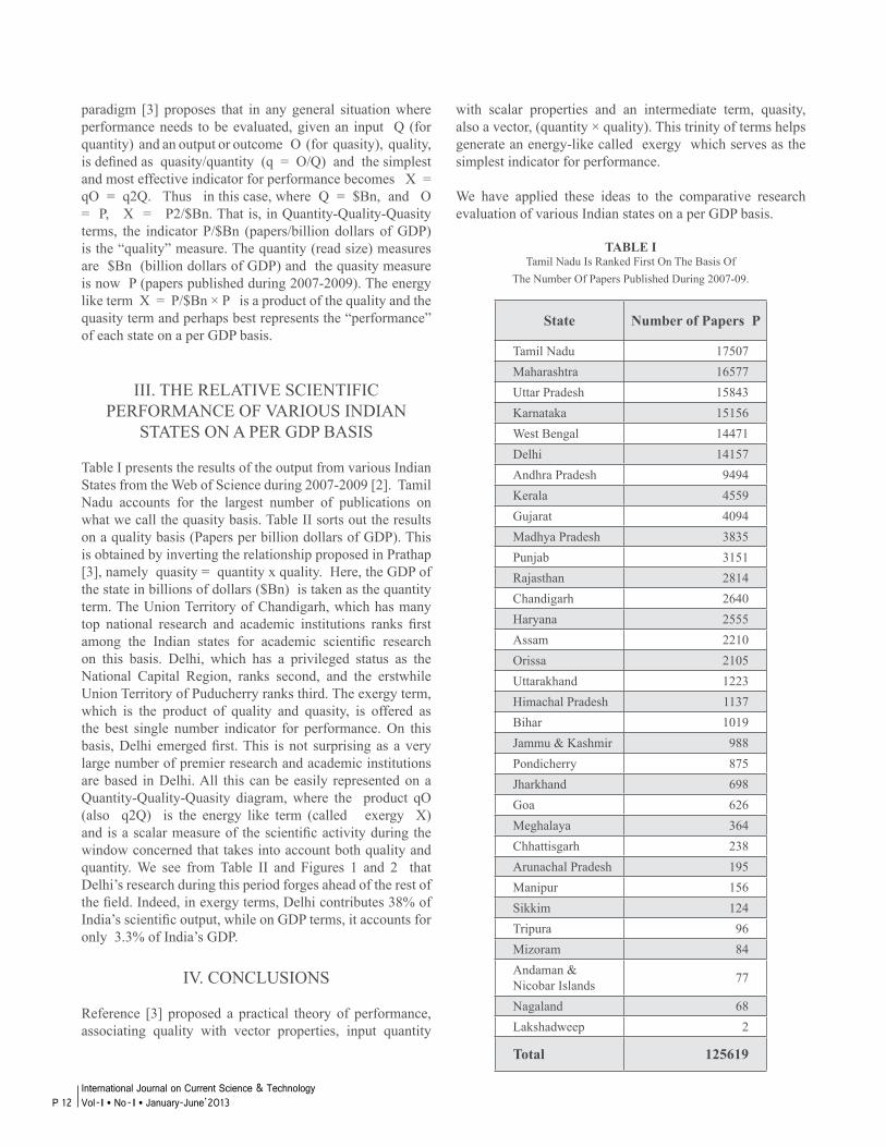
Table I presents the results of the output from various Indian States from the Web of Science during 2007-2009 [2]. Tamil Nadu accounts for the largest number of publications on what we call the quasity basis. Table II sorts out the results on a quality basis (Papers per billion dollars of GDP). This is obtained by inverting the relationship proposed in Prathap [3], namely quasity = quantity x quality. Here, the GDP of the state in billions of dollars ($Bn) is taken as the quantity term. The Union Territory of Chandigarh, which has many top national research and academic institutions ranks first among the Indian states for academic scientific research on this basis. Delhi, which has a privileged status as the National Capital Region, ranks second, and the erstwhile Union Territory of Puducherry ranks third. The exergy term, which is the product of quality and quasity, is offered as the best single number indicator for performance. On this basis, Delhi emerged first. This is not surprising as a very large number of premier research and academic institutions are based in Delhi. All this can be easily represented on a Quantity-Quality-Quasity diagram, where the product qO (also q2Q) is the energy like term (called exergy X) and is a scalar measure of the scientific activity during the window concerned that takes into account both quality and quantity. We see from Table II and Figures 1 and 2 that Delhi’s research during this period forges ahead of the rest of the field. Indeed, in exergy terms, Delhi contributes 38% of India’s scientific output, while on GDP terms, it accounts for only 3.3% of India’s GDP.
IV. CONCLUSIONS
Reference [3] proposed a practical theory of performance, associating quality with vector properties, input quantity
with scalar properties and an intermediate term, quasity, also a vector, (quantity × quality). This trinity of terms helps generate an energy-like called exergy which serves as the simplest indicator for performance.
We have applied these ideas to the comparative research evaluation of various Indian states on a per GDP basis.
TABLE ITamil Nadu Is Ranked First On The Basis Of
The Number Of Papers Published During 2007-09.
State Number of Papers P
Tamil Nadu 17507Maharashtra 16577Uttar Pradesh 15843Karnataka 15156West Bengal 14471Delhi 14157Andhra Pradesh 9494Kerala 4559Gujarat 4094Madhya Pradesh 3835Punjab 3151Rajasthan 2814Chandigarh 2640Haryana 2555Assam 2210Orissa 2105Uttarakhand 1223Himachal Pradesh 1137Bihar 1019Jammu & Kashmir 988Pondicherry 875Jharkhand 698Goa 626Meghalaya 364Chhattisgarh 238Arunachal Pradesh 195Manipur 156Sikkim 124Tripura 96Mizoram 84Andaman & Nicobar Islands 77
Nagaland 68Lakshadweep 2
Total 125619
P 12International Journal on Current Science & Technology Vol - I l No- I l January-June’2013
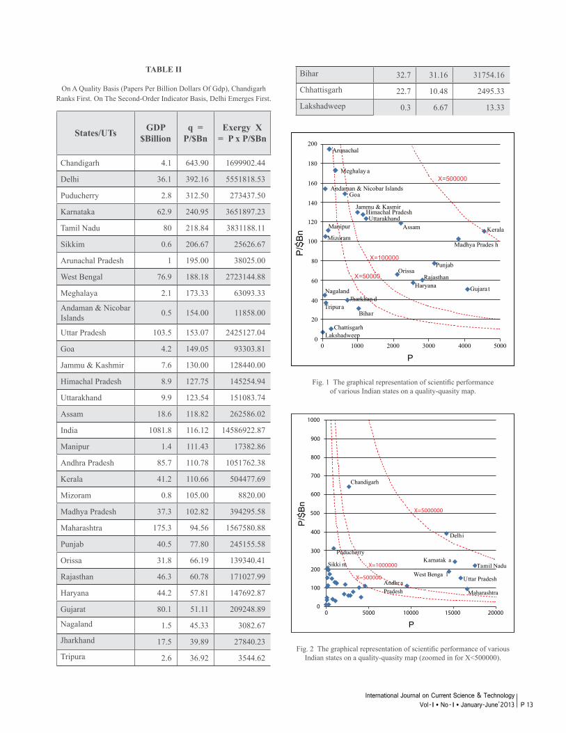
TABLE II
On A Quality Basis (Papers Per Billion Dollars Of Gdp), Chandigarh Ranks First. On The Second-Order Indicator Basis, Delhi Emerges First.
States/UTs GDP $Billion
q = P/$Bn
Exergy X = P x P/$Bn
Chandigarh 4.1 643.90 1699902.44
Delhi 36.1 392.16 5551818.53
Puducherry 2.8 312.50 273437.50
Karnataka 62.9 240.95 3651897.23
Tamil Nadu 80 218.84 3831188.11
Sikkim 0.6 206.67 25626.67
Arunachal Pradesh 1 195.00 38025.00
West Bengal 76.9 188.18 2723144.88
Meghalaya 2.1 173.33 63093.33
Andaman & Nicobar Islands 0.5 154.00 11858.00
Uttar Pradesh 103.5 153.07 2425127.04
Goa 4.2 149.05 93303.81
Jammu & Kashmir 7.6 130.00 128440.00
Himachal Pradesh 8.9 127.75 145254.94
Uttarakhand 9.9 123.54 151083.74
Assam 18.6 118.82 262586.02
India 1081.8 116.12 14586922.87
Manipur 1.4 111.43 17382.86
Andhra Pradesh 85.7 110.78 1051762.38
Kerala 41.2 110.66 504477.69
Mizoram 0.8 105.00 8820.00
Madhya Pradesh 37.3 102.82 394295.58
Maharashtra 175.3 94.56 1567580.88
Punjab 40.5 77.80 245155.58
Orissa 31.8 66.19 139340.41
Rajasthan 46.3 60.78 171027.99
Haryana 44.2 57.81 147692.87
Gujarat 80.1 51.11 209248.89
Nagaland 1.5 45.33 3082.67
Jharkhand 17.5 39.89 27840.23
Tripura 2.6 36.92 3544.62
Bihar 32.7 31.16 31754.16
Chhattisgarh 22.7 10.48 2495.33
Lakshadweep 0.3 6.67 13.33
Fig. 1 The graphical representation of scientific performanceof various Indian states on a quality-quasity map.
Fig. 2 The graphical representation of scientific performance of various Indian states on a quality-quasity map (zoomed in for X<500000).
P 13International Journal on Current Science & Technology
Vol - I l No- I l January-June’2013
200
180
160
140
120
100
80
60
40
20
0
Arunachal
Meghalay a
Andaman & Nicobar IslandsGoa
Jammu & KasmirHimachal PradeshUttarakhand
AssamManipur
MizoramKerala
Madhya Prades h
PunjabOrissa
RajasthanHaryana Gujara tNagaland
Jharkhan dTripura
Bihar
ChattisgarhLakshadweep
P
X=500000
X=100000
X=50000
P/SB
n
0
1000 2000 3000 4000 5000
1000
900
800
700
600
500
400
300
200
100
0
P/SB
n
0 5000 10000
15000
20000
P
Chandigarh
Delhi
Puducherry
Sikki mKarnatak a
Tamil Nadu
Andhr aPradesh
West Benga lUttar Pradesh
Maharashtra
X=5000000
X=1000000
X=500000

IV REFERENCES
[1] J. D. Bernal, The Social Function of Science, London, England: George Routledge & Sons, 1939.
[2] K. C. Garg, and S. Kumar, “Scientometric profile of Indian Science as seen through Web of Science
P 14International Journal on Current Science & Technology Vol - I l No- I l January-June’2013
during 2007-2009,” Indian S&T Report, CSIR- National Institute for Science, Technology and Development Studies, India.
[3] G. Prathap, “Quasity, when quantity has a quality all of its own - toward a theory of performance,” Scientometrics., vol. 88, pp. 555-562, 2011.
IMBALANCE OF TECHNICAL EDUCATIONIN THE NORTH EAST INDIA AND ITS EFFECTS
Sainkupar Marwein Mawiong#
# Department of Basic Sciences & Social Sciences, School of Technology North Eastern Hill University
Mawlai Umshing, Shillong, Meghalaya, Pincode: 793022E-mail : [email protected]
ABSTRACT
Technical education is supposed to be the vital components in the overall holistic development of any region. This paper will highlight the importance of technical education. The different model adopted in India to impart Technical Education. The distribution of different technical education institutes in various part of the country. The main parts of this paper are about the imbalance of Technical education in North East India and its effects.
Keywords: Technical Education, North East India, Imbalance, Holistic Development.
I. INTRODUCTION
According to AICTE Act “Technical Education” means as in [2] programmes of education, research and training in the fields of Engineering & Technology, Architecture, Town planning & Management, Pharmacy & Applied Arts and Crafts and such other programmes or areas as the Central Government may declare in consultation with the council by a Gazette notification.
Technical education in India was initiated in the mid 19th Century. It start to gain pace in the 20th century with the set up of constitution of Technical Education Committee of the Central University Board of Education (CABE) in 1943.Preparation of sergeant Report in 1944 and Formation of All India Council of Technical Education (AICTE) in 1945 as in [2].
Slowly the Government started to establish new institute with world class standards like the IIT (Indian Institute of Technology) and IIM (Indian Institute of Management) to bridge the gap with the other developed nations. Engineers from India are being known worldwide and their demand has increase considerably but access of Technical education to the rural populace is still a distant dream. There is also a regional imbalance in engineering education establishments. Most of the Engineering colleges are located in Andhra Pradesh,
Karnataka, Maharashtra and Tamil Nadu which does not augur well for the balanced socio-economic development of the country as in [2].
In India technical education has been booming of late. Earlier it was dream-come-true for only a handful, but today a popular choice for lakhs of students. In the current academic year and in Tamil Nadu alone 85 new self-financing engineering colleges were approved by AICTE and the total number is 444, second to Andhra Pradesh (523). The five southern states account for 69 per cent of 8.19 lakh students enrolled in 2,297 engineering colleges across the country as in [5].
Obviously the courses being offered have almost quadrupled recently. In Anna University itself from just three basic branches known as Civil, Electrical and Mechanical (Soil, Coil and Oil branches), it has expanded to 41 courses in UG and beyond 100 courses in PG. New and emerging areas like Biotechnology, Nanotechnology, Ocean Engineering and Climate Change, Environmental Engineering, etc., are also added as in [5].
States such as Uttar Pradesh, Rajasthan and Orissa together account for just 14 per cent of India‘s technical colleges. This regional imbalance and quality are now the grave concerns as in [5].
II. STRUCTURE OF TECHNICAL EDUCATION IN INDIA
Different patterns of funding and controls of technical institutions have resulted in different organisational structures of technical education, which may be grouped according to the types of institutions such as the Indian Institutes of Technology (IITs), Regional Engineering Colleges (RECs), Government Colleges/Polytechnics, Government - Aided Colleges/Polytechnics, Self-Financing Private Colleges/Polytechnics and Institutes awarding PGDBM/PGDCA. Indian Institutes of Technology (IITs), and Indian Institutes of Management (IIMs), have been set up as institutions
P 15International Journal on Current Science & Technology
Vol - I l No- I l January-June’2013
of national importance and they enjoy greater autonomy in matters of academics and administration. In addition to the formal system of education given in the engineering colleges and polytechnics, there are a number of professional bodies which conduct their own examinations for serving professionals and award certificates and diplomas which are recognised to be equivalent to diploma/degree awarded through the formal education system.
In the case of computer education, the Department of Electronics has an elaborate system of giving accreditation to computer institutes in non-formal sector for conducting of specified levels of courses - DOEACC level “O”, “A”, “B”, & “C” subject to their meeting of well defined norms and criteria. In the case of pharmacy and architecture education, the Pharmacy Council and Council of Architecture, respectively, also have statutory obligations and the AICTE works in close cooperation with these Councils.
Since technical education determines the development & socio economic condition of a nation, there is greater need for high quality technical education to produce technically skilled manpower in India.
Technical education is imparted at three different levels in India.
i. Industrial training institutes (ITI), which runs trade courses for skilled workers.
ii. Polytechnics, they run diplomas to produce middle level (supervisory level) technicians.
iii. Engineering colleges, which conduct under graduate programme.
In the Indian system, the completion of senior secondary examination is the stage from where higher education begins (ten years of primary and secondary education plus two years of higher secondary education). The first degree, the bachelor’s degree is obtained after three years of study in the case of science and liberal arts and four years in the case of engineering and technology. The Master’s degree programme was of two year’s duration earlier but is currently of one and a half year duration. The research degree (Ph.D) takes variable time but can be completed in three years [3].In addition to degree courses in engineering and technology a number of discipline-oriented and certificate courses are also available. Their range is wide, some being undergraduate diploma courses and others postgraduate courses with a duration of one to three years as in [3].
III. DISTRIBUTION OF DIFFERENT TECHNICAL EDUCATION INSTITUTES IN
DIFFERENT STATES
[2] Since Independence in 1947, the Technical Education System has grown into a fairly large-sized system, offering opportunities for education and training in a wide variety of trades and disciplines at certificate, diploma, degree, postgraduate degree and doctoral levels in institutions located throughout the country. Even though the system boasts o institutions comparable to the best in the world, quality of education offered in majority of institutions leaves much to be desired.
In the year 1947-48, the country had 38-degree level institutions with intake capacity of 2500 and 53 diploma level institutions with intake capacity of 3670. The intake for postgraduates was 70.
There was rapid expansion of the system in the next 20 years. By 1967-68, the number of degree level institutions had increased to 137 with intake capacity of 25,000; and for diploma to 284 institutions with intake capacity of 47,000.
In the year 2000, the total size of the system had increased to 4146 institutions with approved intake capacity of 544,660. These include 838 engineering degree institutions with admission capacity of 232,000 students; and 1224 engineering diploma institutions with admission capacity of 188,000.
Approximately, two-thirds of these institutions were in the private sector. Postgraduate education was being offered in 246 institutions with admission capacity of 21,460.
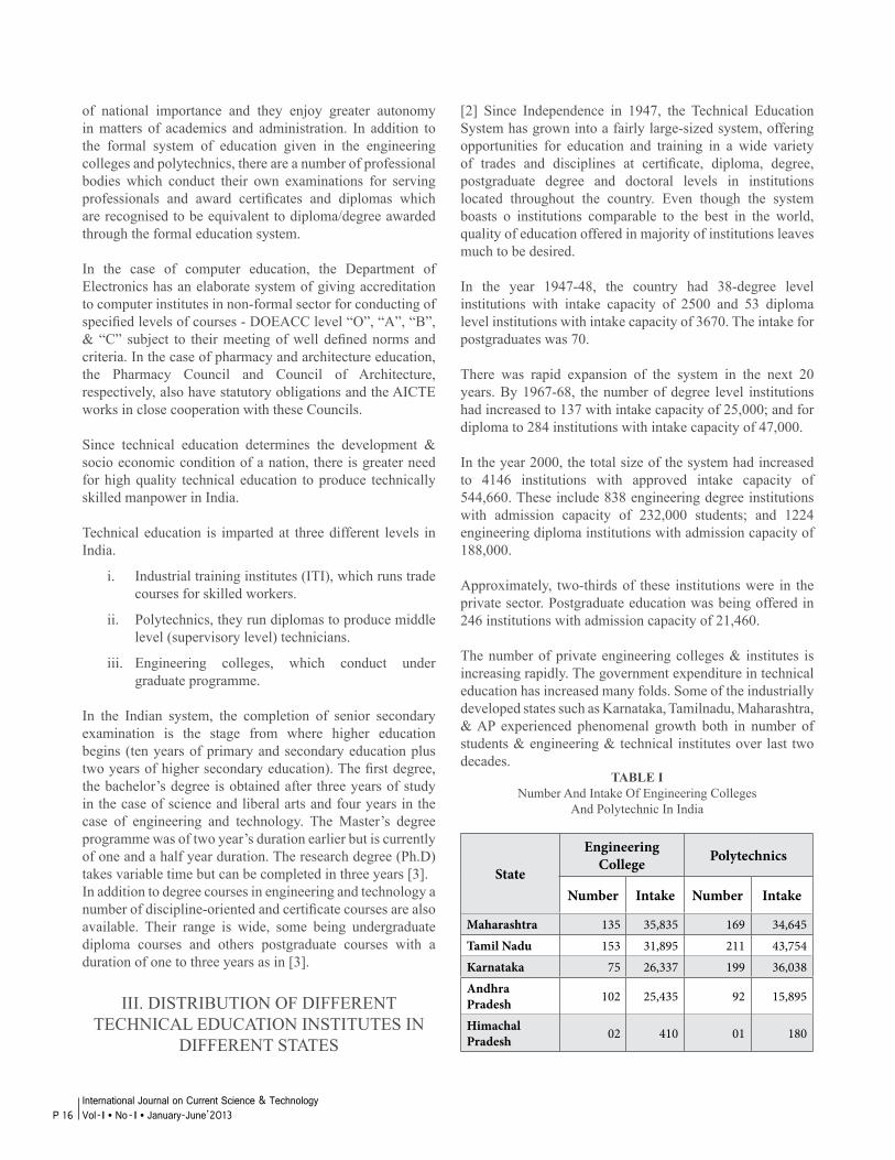
The number of private engineering colleges & institutes is increasing rapidly. The government expenditure in technical education has increased many folds. Some of the industrially developed states such as Karnataka, Tamilnadu, Maharashtra, & AP experienced phenomenal growth both in number of students & engineering & technical institutes over last two decades.
TABLE INumber And Intake Of Engineering Colleges
And Polytechnic In India
State
Engineering College Polytechnics
Number Intake Number Intake
Maharashtra 135 35,835 169 34,645Tamil Nadu 153 31,895 211 43,754Karnataka 75 26,337 199 36,038Andhra Pradesh 102 25,435 92 15,895
Himachal Pradesh 02 410 01 180
P 16International Journal on Current Science & Technology Vol - I l No- I l January-June’2013

Assam 03 660 10 1,318North-Eastern States 05 860 11 1,490
Bihar 12 2,635 28 3,983Gujarat 20 5,885 39 9,005
Sources: in [3]
If we look at the Eleventh Five Year plan it mainly focused on increasing intake capacity (GER), starting new educational institutions, enhancing the capacity of existing ones, starting new programmes etc [4].
There are 81 centrally funded institutes of technical & science education (CFTIs) out of which 30 were created during the XI FYP [4]:
TABLE IINumber Of Centrally Funded Institutions
Centrally Funded Institutions Number of Institutions
Indian Institutes of Technology (IITs) 15(8)
Indian Institutes of Management (IIMs) 13(7)Indian Institute of Sciences (IISc.) 1Indian Institutes of Sciences Education & Researchv(IISERs)
5(3)
National Institutes of Technology (NITs) 30(10)Indian Institutes of Information Technology (IIITs)
4
National Institutes of Technical Teachers Training & Research (NITTTRs)
4
Others 9(8)School of Planning & Architecture(SPAs)-3, Indian School of Mines(ISM), North-East Regional Institute of Science 7 Technology (NERIST), National Institute of Industrial Engineering (NITIE), National Institute of Foundry & Forge Technology(NIFFT), Sant Longowal Institute of Engineering & Technology (SLIET), Central Institute of Technology (CIT).TOTAL 81(30)
Sources: in [4]
In addition to the above the Central Government is implementing the following schemes/programmes: as in [4]
• National Mission on Education through ICT (NMEICT)
• Technical Education Quality Improvement Programme assisted by the World Bank (TEQIP)
• Indian National Digital Library for Science & Technology (INDEST)
• Sub-mission on Polytechnics under coordinated action for skill development: The objective of the scheme is to enhance employment oriented skilled manpower through polytechnic. Under the scheme, financial assistance is provided to the State/UT Government for setting up of 300 new Polytechnics in unserved and neglected districts of the country. Out of 300 Polytechnics, financial assistance has been provided for setting up of new Polytechnics in 277 districts. In addition financial assistance is provided to the existing Government/Government aided Polytechnics for strengthening of infrastructure facility, so far 500 polytechnic have been provided for assistance of Rs. 10/20 lakhs each.
• Setting up of 20 new Indian Institute of Information Technology (IIITs): The Ministry of Human Resource Development (MHRD) is setting up 20 new Indian Institutes of Information Technology (IIITs) to address the increasing skill challenges of the Indian IT industry on a Public Private Partnership (PPP) basis. As per the approved scheme, the partners in setting up the IIITs would be the Ministry of Human Resource Development (MHRD), Government of the respective States where each IIIT will be established, and the industry. The capital cost of each IIIT would be Rs. 128.00 crore to be contributed in the ratio of 50:35 : 15 by the Central Government, the State Government, and the industry respectively. The project is targeted to be completed in nine years from 2011-12 to 2019-20. During the current year it is expected that 5 such institutions would be set up. The rest would be taken in the XII FYP.
• Expansion in the AICTE approved institutions: In addition to the unprecedented expansion in the numbers of the premier CFTI s like IITs , IIM, NITs, IISERs etc , the number of AICTE approved institutions in the country during the period has almost doubled which rose from 4491 in 2006-07 to 8361 in 2011-12 and annual intake from 907822 in 2007-08 to 2046611 in 2011-12. Similarly, number of polytechnics has increased with corresponding rise in intake from 417923 in 2007-08 and 1083365 in 2010-11.
The growth of the institutions for the last five years and the number of students’ intake is as below:
TABLE IIIINTAKE CAPACITY
Year Number of Institutions
Added in year
Total student intake
for UG/PG
Total student
intake for Polytechnic
P 17International Journal on Current Science & Technology
Vol - I l No- I l January-June’2013
2006-07 4491 1712007-08 4885 384 907822 4179232008-09 6230 1345 1139116 6109032009-10 7361 1131 1408807 8504812011-12 8361 357 2046611 987929*
*all polytechnics have not entered data.Sources: in [4]
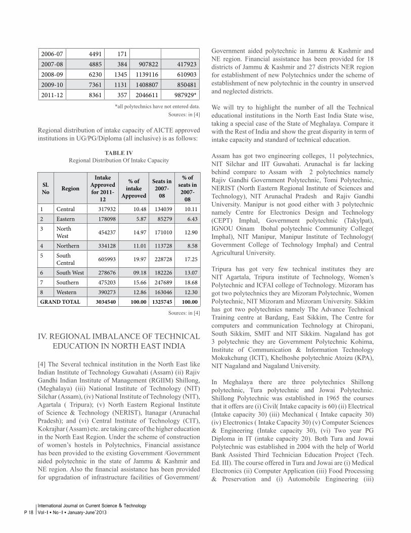
Regional distribution of intake capacity of AICTE approved institutions in UG/PG/Diploma (all inclusive) is as follows:
TABLE IVRegional Distribution Of Intake Capacity
Sl. No Region
Intake Approved for 2011-
12
% of intake
Approved
Seats in 2007-
08
% of seats in 2007-
081 Central 317932 10.48 134039 10.112 Eastern 178098 5.87 85279 6.433 North
West 454237 14.97 171010 12.90
4 Northern 334128 11.01 113728 8.585 South
Central 605993 19.97 228728 17.25
6 South West 278676 09.18 182226 13.077 Southern 475203 15.66 247689 18.688 Western 390273 12.86 163046 12.30GRAND TOTAL 3034540 100.00 1325745 100.00
Sources: in [4]
IV. REGIONAL IMBALANCE OF TECHNICAL EDUCATION IN NORTH EAST INDIA
[4] The Several technical institution in the North East like Indian Institute of Technology Guwahati (Assam) (ii) Rajiv Gandhi Indian Institute of Management (RGIIM) Shillong, (Meghalaya) (iii) National Institute of Technology (NIT) Silchar (Assam), (iv) National Institute of Technology (NIT), Agartala ( Tripura); (v) North Eastern Regional Institute of Science & Technology (NERIST), Itanagar (Arunachal Pradesh); and (vi) Central Institute of Technology (CIT), Kokrajhar ( Assam) etc. are taking care of the higher education in the North East Region. Under the scheme of construction of women’s hostels in Polytechnics, Financial assistance has been provided to the existing Government /Government aided polytechnic in the state of Jammu & Kashmir and NE region. Also the financial assistance has been provided for upgradation of infrastructure facilities of Government/
Government aided polytechnic in Jammu & Kashmir and NE region. Financial assistance has been provided for 18 districts of Jammu & Kashmir and 27 districts NER region for establishment of new Polytechnics under the scheme of establishment of new polytechnic in the country in unserved and neglected districts.
We will try to highlight the number of all the Technical educational institutions in the North East India State wise, taking a special case of the State of Meghalaya. Compare it with the Rest of India and show the great disparity in term of intake capacity and standard of technical education.
Assam has got two engineering colleges, 11 polytechnics, NIT Silchar and IIT Guwahati. Arunachal is far lacking behind compare to Assam with 2 polytechnics namely Rajiv Gandhi Government Polytechnic, Tomi Polytechnic, NERIST (North Eastern Regional Institute of Sciences and Technology), NIT Arunachal Pradesh and Rajiv Gandhi University. Manipur is not good either with 3 polytechnic namely Centre for Electronics Design and Technology (CEPT) Imphal, Government polytechnic (Takylpat), IGNOU Oinam Ibohal polytechnic Community College( Imphal), NIT Manipur, Manipur Institute of Technology( Government College of Technology Imphal) and Central Agricultural University.
Tripura has got very few technical institutes they are NIT Agartala, Tripura institute of Technology, Women’s Polytechnic and ICFAI college of Technology. Mizoram has got two polytechnics they are Mizoram Polytechnic, Women Polytechnic, NIT Mizoram and Mizoram University. Sikkim has got two polytechnics namely The Advance Technical Training centre at Bardang, East Sikkim, The Centre for computers and communication Technology at Chiropani, South Sikkim, SMIT and NIT Sikkim. Nagaland has got 3 polytechnic they are Government Polytechnic Kohima, Institute of Communication & Information Technology Mokukchung (ICIT), Khelhoshe polytechnic Atoizu (KPA), NIT Nagaland and Nagaland University.
In Meghalaya there are three polytechnics Shillong polytechnic, Tura polytechnic and Jowai Polytechnic. Shillong Polytechnic was established in 1965 the courses that it offers are (i) Civil( Intake capacity is 60) (ii) Electrical (Intake capacity 30) (iii) Mechanical ( Intake capacity 30) (iv) Electronics ( Intake Capacity 30) (v) Computer Sciences & Engineering (Intake capacity 30), (vi) Two year PG Diploma in IT (intake capacity 20). Both Tura and Jowai Polytechnic was established in 2004 with the help of World Bank Assisted Third Technician Education Project (Tech. Ed. III). The course offered in Tura and Jowai are (i) Medical Electronics (ii) Computer Application (iii) Food Processing & Preservation and (i) Automobile Engineering (iii)
P 18International Journal on Current Science & Technology Vol - I l No- I l January-June’2013
Architectural Assistantship (iii) Costume Design & Garment Technology with an intake capacity of 30 each. These entire polytechnic are affiliated to Meghalaya State Council for Technical Education created in 1992 through an act called Meghalaya State Council for Technical Education Act, 1993. “ISO 9001: 2000 certified”. There is no state government degree engineering college.
North Eastern Hill University is also offering degree in Technology with the introduction of two new departments in 2006 they are IT & ECE and the intake capacity is 60 each. There is a plan that in 2013 three new branches Biomedical, Energy and Nanotechnology will be open up. To boost the management studies in 2004 IIM Shillong was established. Apart from all these institutions there are also three new private engineering colleges they are UTM (University of Technology Management), USTM (University of Science and Technology Meghalaya) and CMJ University.
The number of intake capacity for polytechnic in Meghalaya is only 380 which is very very less is comparison with the other parts of the country. Regarding degree technical education only the Private University and the Central Government University is offering degree in Engineering in which the total intake capacity is approximately 700 which is nothing in comparisons with the other States. The current picture of technical education in Meghalaya is very worst as there is no State Government Engineering Colleges which prevent a student from weaker economically background to pursue higher studies in engineering as the option for is very limited.
If we look at the Eastern part of India as a whole we can see from Table IV that the Intake approved for 2011-12 is only 178098 and the percentage of intake Approved is 5.87 percent which is pathetic in comparison with the other region. In the year 2007-08 the situation is almost the same. Even though North Eastern States is a conglomeration of seven states but studying from Table I show us that the number of Technical institutes in North Eastern States is very less compare to any other developed states of India.
So a student from North East has got less opportunities and option to pursue the careers that he dream of as there is very less seats and the variety of course offered are not so goods as compare to the mainstream India. This ultimately affect the development of the region as there is very less technical people who are able to contribute to the progress and the over all development of the region.
There has been phenomenal growth of technical institutions during past three decades however it has resulted in a regional imbalance of the technical education system in the Country. In order to overcome the regional imbalance, AICTE has given
permit for second shift of engineering college in an existing engineering college in those states where the number of seats available in engineering colleges per lakh of population is less than all India average without additional investment and also to utilize the existing resources in optimal manner and to minimize the cost of education which will help in the
• Reduction of regional imbalance by encouraging existing technical institutions to start second shift in those states where the number of seats available in engineering colleges per lakh of population are less than all India average and in institutions which are exclusively set up for women;
• Optimal utilization of resources
• Reduction cost of education per student.
[6] The spread of technical education suffers from regional imbalances. After privatisation of technical education, a large number of new private colleges appeared in a few’ states while many states that urgently needed development could not attract such institutes. A balanced growth of technical education in the country is desirable. Even within the same state, there are intrastate regional imbalances with Pareto’s Law of mal-distribution leading to ‘vital few and ‘ ignored many regions where these new colleges have emerged. While it is understandable that certain locational advantages’ will attract more private participation than others, yet the under-represented regions do need either government supported initiatives or Public-Private Partnership ( PPP) or the state offers a set of packages as incentives to private academic investors to set up quality institutions in those regions. The con-cept of special knowledge /ones’ and knowledge villages”, developed by the state can be set up. These can attract private investments.
IV. CONCLUSIONS
The strength of technical education system in India is that it has got a very rich and learned education heritage, very good primary education which provides a very strong base. Indian education system Moulds the growing minds with huge amount of information and knowledge. Indian education system gives the greater exposure to the subject knowledge, Indians are rich in Theoretical knowledge .India has abducted strength of resources and man power (NASA, MAC), cost of education is very low, number of higher education institutions in India is more compare to developed countries, Indians are interceded in normal education and higher education [2].
The weakness of Indian technical education system is that it lacks of adequate up-gradation of Curriculum. There is no benchmark and no common course content and no
P 19International Journal on Current Science & Technology
Vol - I l No- I l January-June’2013
common exam procedure national wide, Lack of specialized courses or modular and rigid curriculum learning considered as one step process. Education is exam oriented. No fixed parameters, Lack of Industry -Institute interaction. lack of multidisciplinary courses. Role of teacher is confined to teaching alone, Lack of policy makers. Mind set of stakeholders, Lack in accepting immediate changes. Learning is job oriented [2].
The opportunities of Technical Education in India are that it has rich resources of human as well as physical. In India enough number of higher education institutions can be set up. Therefore, we can produce more and highly qualified students, fulfilling students’ demands by providing enhanced quality of education. Producing enough number of technically skilled outputs, by giving more Autonomy, Curriculum should be made more realistic, practically biased and job oriented, Students will be regarded more as a customer. To provide highly technically skilled labour to the country [2].
Similarly the threats of Indian technical education system are Lack of interest and interaction from the industry in developing and collaborating in the research field, threat from within of deteriorating standards of education due to lack of benchmark in terms of quality of institutions, Loss of quality standards by technical institutions as more and more students opt for education abroad, Lack of team work. Peoples’ attitude, who failed to work collectively on a common minimum platform [2] [1].
Last but not the least the biggest threat for technical education in India is Regional Imbalance as the Region which has got very few technical institutes will always be behind in terms of development as there are few technical people who will be the driving force in shaping the future of that particular region. Eventually the Region will be underdeveloped and the people will feel left out and feel that they are being denied their fair share of development. So this will lead to unrest as we have seen with so many parts of India. Which ultimately drag the nation two steps backwards instead of two steps forward.
ACKNOWLEDGMENT
I will like to thank Dr B. Bhuyan Head of the Department Information Technology, North Eastern Hill University, Shillong for kindly informing me about this Regional
Congress which is going to be held in NIT Arunachal Pradesh and encourage us all faculty members from School of Technology to participate in this Regional Congress.
REFERENCES
[1] S.K.Saha and S.Ghosh, Engineering Education in India: Past, Present and Future, Propagation, A Journal of Science Communication, Vol. 2, No. 2, July, 2011.
[2] Shivani and S. Khurana. Technical Education in India Present Scenario, International Journal of Research in Economics and Social Sciences, Vol.2, Issue. 10, October, 2012. ISSN:2249-7382.
[3] Pursuit and Promotion of Sciences. “Engineering and Technical Education”, Chapter VI. [Online] Availabel: http://www.iisc.ernet.in/insa/ch6.pdf
[4] Report of the Working Group on Technical Education for the XII Five year plan [Online] Available : http:// planningcommission.nic.in/aboutus/committee/wrkgrp12/ hrd/wg_te.pdf
[5] The Hindu, “Technical education Challenges ahead”, issue: 2nd February, 2010
[6] P. Vrat, Impart Quality in Technical Education, SME World[Online] Available : http://www.smeworld.org/story/ features/impart-quality-in-technical-education.php
[7] P.R.Dasgupta, Technical Education Contributing to Industrial Development, Govt of India [Online] Available: http://pib.nic.in/feature/fe0199/f0501991.html
[8] D.K.Nayak and T.V. Mohite- Patil, Impact of Globalization & IT Revolution on Technical Education, [Online] Availble: http://dspace. v p m t h a n e . o r g : 8 0 8 0 / j s p u i / b i t s t r e a m / 1 2 3 4 5 6 7 8 9 / 1 2 6 3 / 1 / I M PA C T % 2 0 O F % 2 0 G L O B A L I Z A T I O N % 2 0 % 2 6 % 2 0 I T % 2 0 R E V O L U T I O N % 2 0 O N % 2 0 TECHNICAL%20EDUCATION.pdf
[9] V.P.Goel, Technical and Vocational Education and Training (TVET) System \ in India for Sustainable Development, Govt Of India [Online] Available: http://www.unevoc.unesco.org/up/India_Country_ Paper.pdf
P 20International Journal on Current Science & Technology Vol - I l No- I l January-June’2013
REVIEW AND SUGGESTIONS FOR REVAMPINGTECHNICAL HIGHER EDUCATION
IN INDIA TO MEET THE CHALLENGES OF FUTURE
Abhinandan Bhunia1, Abhirup Bhunia2, Swarnendu Kr. Chakraborty3, Pinaki Chakraborty3, Rajat Subhra Goswami3, Nabakumar Pramanik3, Mohit Kumar De3, Pralay Kumar Samanta3, Chandan Tilak Bhunia3
1 Microsoft Corporation, USA; 2 G-4, Garden Green Aprts, 184 Bansdroni Place, Kolkata-700070, 3 National Institute of Technology, Arunachal Pradesh, Yupia-791112, India
I. NTRODUCTION
Many studies have authoritatively established that the most sufferers from the globalization forces are the marginalized developing and poor nations. With a pursue to make globalization a sustainable strategy for the developing nations, it has been internationally recognized that improved higher education, both in quantity and quality should be one of the sound strategies for the developing nations for the competitive advantages. Historically this is also a conclusive and decisive rule of development as “the real wealth of a nation is its people” and more specifically so in today’s knowledge based society where “Knowledge is Power.” UNESCO (United Nations Educational, Social and Cultural Organization) [1] puts it as “Without improved human capital, countries will inevitable fall behind and experience intellectual and economic marginalization and isolation ...... In the developed World education is a major political priority.” The hard reality is that India is yet to attain the international status of higher education. Making India developed economy without developed higher education will no way be a sustainable strategy.
Since the adoption of liberalization, privatization & globalization in 1990s, India’s Technical Higher Education (THE) both at UG & PG has taken a new shape never-seen-before [2]. Private investment and participation in THE, primarily when the Government neither can establish new colleges & universities to cater the demand for enrolment in THE for years after years nor can afford to do so, has become a decisive factor to reckon with. In such a new scenario, emerges a role to critically reviewing the THE in a holistic approach. It is particularly essential and of paramount necessary in view of the fact that there is seen hardly any planned strategy to guide and regulate THE so as to be country specific, productive and distinctive beyond which the growth has neither any meaning nor any relevance. There is no
meaning to be a follower and always being lagged. Need of the hour and challenge is become leader & innovative to restructuring and redressing THE to judiciously make it country specific and delivery system. After all, the socio-economic development has direct relevancy to THE. The big challenge is just not to open the avenues for open economy, but to regulate same for creating gracious opportunities and scope beyond the business. After all THE is supposed to be a human resource generation in a process of man making in building nation.
A decisive and well-timed research has therefore been undertaken to review the existing THE. A comprehensive and critical review in this respect has been done in the research.
The research aimed to study:
• Quantity & quality dimension of THE• Imbalances if any in THE in respect of subjects, geography• Deliverables & applicability • Lacks & lags in comparison with international standard.
Based on the study as proposed above, several suggestions in relate to modifications of systems, regulations and structures are worked out in this research.
II. QUANTITY AND QUALITY IN THE
It is decisively established that improved and more human resource generation shall be the sound strategy for competitive advantages in liberalized economy. The strategy is well adopted in the developed countries. The inclusive analysis reveals that in developed countries the generation of human resource is at par and in pace with that of physical infrastructural development. In fact, human generation is
P 21International Journal on Current Science & Technology
Vol - I l No- I l January-June’2013
apparently and practically assumed as a social service sector in the developed countries. In theory, the same is adopted in developing countries but in practice it is far behind that in practice in developing countries. Quantity wise and quality wise scant initiative and approach is noticed in generation of human resource in all the developing countries. The fact was well studied in several various researches [3-7]. The thesis of development is nothing but judicious and wide application of science and technology in the development process. The real difference between the developing and the developed is nothing but science and technology.
Under the scenario an approach is made to critically analyze the position of India in respect of human resource generation, in comparison with other countries, particularly with developed countries.
Fig. 1 and 2 represent the comparative study of universities versus population and population per university against educational expenditure in different countries throughout the world. Fig. 3 shows the comparison of total Government spending across all areas of education over different countries in the world.
India has made progress in terms of increasing primary education attendance rate and expanding literacy to approximately two thirds of the population. India’s improved education system is often cited as one of the main contributors to the economic rise of India. Much of the progress especially in Higher education, Scientific research has been credited to various public institutions.
To gain a better overview of educational resourcing, other resourcing indicators such as government spending per student and pupil teacher ratio should also be consulted.A comparative study of population in core versus GDP versus human development index in the world has been represented in Fig 4. The Comparing educational spending with GDP can be an indicator of the importance of education according to government policy makers. However this indicator can be misleading if the GDP is significantly higher or lower than average.
The Human Development Index (HDI) is a composite statistic used to rank countries by level of “human development”, taken as a synonym of the older terms “standard of living” and/or “quality of life”, and distinguishing “very high human development”, “high human development”, “medium human development”, and “low human development” countries.
After participation in globalization, the quality and productivity of India’s research is on decline state if the share of world’s total publication is considered. In 1990-2000, the growth in the world’s publication share was 17.64%, -27.45%
and -12.61% respectively in Japan, Russia and India. A world account is shown in Table 1. This clearly indicates the India’s failure in adaptability to changing global higher education process and to utilize the effectiveness to become leader, although talent is no dearth in India.
Earlier comprehensive in respect to quantity & quality of THE can be seen in [8]. Our present findings are in cohesion with the findings of previous study.
II.1. INFERENCE BASED ON STUDY AS ABOVE:
The number of universities/institutes in India is less both in absolute term as well as in terms of per population in the world.The educational expenditure survey indicates that the expenditure per university in higher education is very poor in India again both in absolute value as well as per population basis in the world.It is also evident that the development is squarely related to more number of universities, more expenditure in education, higher GDP and better human development index.
III. IMBALANCES IN TECHNICAL HIGHER EDUCATION
Several imbalances in technical higher education have been studied authoritatively elsewhere [9, 10]. We like to undertake studies to reexamine the imbalances if any with respect to intake capacity in different disciplines, and the distributions of sanctioned intake over institutes of different states. We iterate that these imbalances are due to unplanned growth of the technical educations in our country, which not only hampering the quality productivity but also the future growth plan and sustainability of technical education so far demand & supply and national development and employment opportunity are concerned.
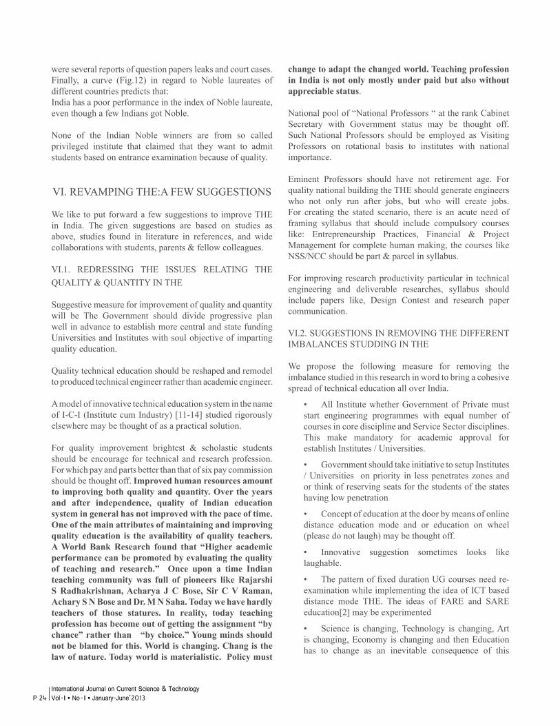
We first study the existing seat capacity of two groups of engineering disciplines. One group is core engineering and another group is of service sector engineering. Core engineering includes the mother engineering disciplines namely Civil Engineering, Mechanical Engineering, and Electrical Engineering. Service sector engineering includes Computer Science & Engineering & Information Technology, Electronics & Communication Engineering and Bio-Technology. Of course Bio-Technology may belong to a hybrid group in engineering. Fig. 5 shows existing intake capacity of different disciplines of two distinct groups. The result is alarming that discipline of core sector are far behind than that of job oriented discipline like Computer Science Engineering & Information Technology. Such un-planned growth & uncontrolled pattern is not only creating huge
P 22International Journal on Current Science & Technology Vol - I l No- I l January-June’2013
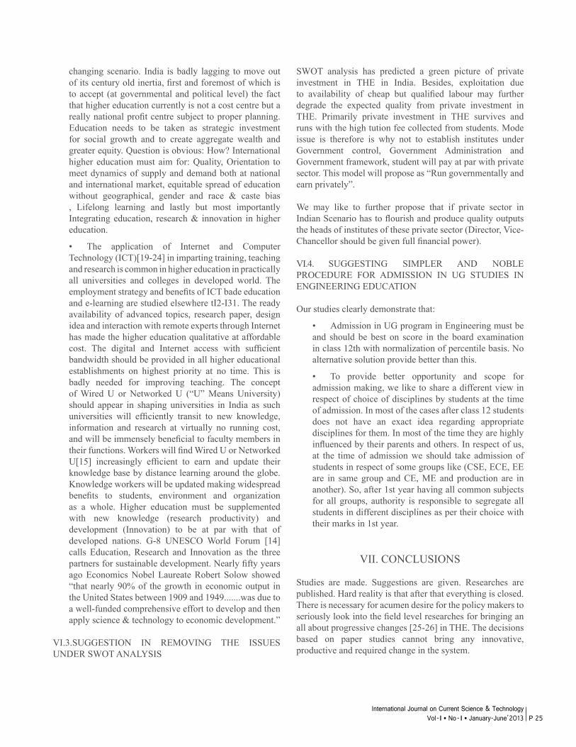
crisis in the demand and the supply of appropriate engineers in national building but also doing academic injustice to the engineering education. This sort of imbalance may seriously hamper the productivity and quality of engineering education and research. This also reflected in Fig. 6, which is for the central universities and institutes of national importance. This shows that the centrally funded institutes are also not planning appropriately for growth of engineering disciplines in equitable, sustainable and developmental manner. This is a matter of great concern and needs remedial measures for correction and improvement.
In Fig. 7 & 8 we study the population per available seat in different disciplines in different states in the country. It is reflected widely and promptly that there is huge imbalance in the available seat over geographical regions all over India. This unequal pattern neither is nether good for national development nor expected. Unequal development and pattern is sometimes the cause of social unrest. Therefore, there is an emerging need for correcting and rectifying the imbalances as studied.
Our observations and study further strengthens the study made in this purpose elsewhere [9, 10].
IV. SWOT ANALYSIS OF PRIVATE INVESTMENT IN THE VERSUS THAT OF
GOVERNMENTAL
For effective analysis and to review, we feel it necessary to have an in depth SWOT analysis of Government versus Private investment in THE. The analysis is made in Table-2 on known perspectives and reports received from stakeholders.
IV.1. INFERENCES
The copying attitude of the developing countries cannot yield good results. The above SWOT analysis clearly demonstrates the fact is that one system cannot be replacement of another system. Therefore there is need of any concern to ensuring quality by copying practices of the developed countries. India needs to devise its own policy to meet the challenges.
V. REVIEWING THE CURRENT NATIONAL DEBATE ON ADMISSION POLICY IN UG
ENGINEERING COURSES
A debate is crippled on the admission procedure to be adopted in the admission to the engineering colleges and universities. The move taken by Ministry of Human Resource
Development to introduce a single admission test and /or simpler procedure for admission in engineering colleges and universities is a well-timed move. Several criticisms, debate on this move are noticed in media. The fundamental question of degrading quality on the move initiated by Ministry of Human Resource Development needs to be examined in totality with critical studies and analysis. This is a paramount importance in view of the untiring protest by various senates and different teaching forum of premier technological universities namely Indian Institutes of Technology. This research has made an attempt to study the relevancy of quality with rank in Joint Entrance Examination made for admission in engineering colleges and universities.
Our parameter of study are university score in B.Tech examination; average score in Physics, Chemistry & Mathematics in 10+2 and AIEEE rank on which admission in engineering colleges and universities are made. The data collection is of the students admitted in 2010-11 sessions and 2011-12 sessions in National Institute of Technology, Arunachal Pradesh.
In this work we have tried to justify the necessity or otherwise of Joint Entrance Examination (referred example is AIEEE rank) for admission in undergraduate engineering examination study. For this purpose we have studied and compared the scores of student’s in two disciplines are Computer Science & Engineering and Electronics & Communication Engineering of university (National Institute of Technology, Arunachal Pradesh) in university rank, class 12 score & AIEEE rank. Our study & comparison are portrayed in Fig. 9, 10 & 11. From the figures it is evident that:
The performance of the students in the university B.Tech examination nearly resembles with that of the (score in PCM) of class 12 examinations.
In certain cases particularly in case of high rank AIEEE students, university score is also high. But the fact is that these students’ PCM rank is also high in class 12 examination.Therefore it is a decisive conclusion that, the score in PCM in board examination may and will be the most appropriate index of quality for admission in undergraduate THE system, rather than conducting separate entrance examination. It may be pertaining to mention here that the conducting of joint entrance examination gives preference to the students of rich families at the cost of merit of the students of poor families. This is because of the fact that merit cannot be judged only by making the students prepare and fittest in a particular structure and orientation of answering in particular question paper setting and examination patterns. Not only that, several unholy practices and money power play sometimes big role in deciding student’s future in joint entrance, as there
P 23International Journal on Current Science & Technology
Vol - I l No- I l January-June’2013
were several reports of question papers leaks and court cases.Finally, a curve (Fig.12) in regard to Noble laureates of different countries predicts that:India has a poor performance in the index of Noble laureate, even though a few Indians got Noble.
None of the Indian Noble winners are from so called privileged institute that claimed that they want to admit students based on entrance examination because of quality.
VI. REVAMPING THE:A FEW SUGGESTIONS
We like to put forward a few suggestions to improve THE in India. The given suggestions are based on studies as above, studies found in literature in references, and wide collaborations with students, parents & fellow colleagues.
VI.1. REDRESSING THE ISSUES RELATING THE QUALITY & QUANTITY IN THE
Suggestive measure for improvement of quality and quantity will be The Government should divide progressive plan well in advance to establish more central and state funding Universities and Institutes with soul objective of imparting quality education.
Quality technical education should be reshaped and remodel to produced technical engineer rather than academic engineer.
A model of innovative technical education system in the name of I-C-I (Institute cum Industry) [11-14] studied rigorously elsewhere may be thought of as a practical solution.
For quality improvement brightest & scholastic students should be encourage for technical and research profession. For which pay and parts better than that of six pay commission should be thought off. Improved human resources amount to improving both quality and quantity. Over the years and after independence, quality of Indian education system in general has not improved with the pace of time. One of the main attributes of maintaining and improving quality education is the availability of quality teachers. A World Bank Research found that “Higher academic performance can be promoted by evaluating the quality of teaching and research.” Once upon a time Indian teaching community was full of pioneers like Rajarshi S Radhakrishnan, Acharya J C Bose, Sir C V Raman, Achary S N Bose and Dr. M N Saha. Today we have hardly teachers of those statures. In reality, today teaching profession has become out of getting the assignment “by chance” rather than “by choice.” Young minds should not be blamed for this. World is changing. Chang is the law of nature. Today world is materialistic. Policy must
change to adapt the changed world. Teaching profession in India is not only mostly under paid but also without appreciable status.
National pool of “National Professors “ at the rank Cabinet Secretary with Government status may be thought off. Such National Professors should be employed as Visiting Professors on rotational basis to institutes with national importance.
Eminent Professors should have not retirement age. For quality national building the THE should generate engineers who not only run after jobs, but who will create jobs. For creating the stated scenario, there is an acute need of framing syllabus that should include compulsory courses like: Entrepreneurship Practices, Financial & Project Management for complete human making, the courses like NSS/NCC should be part & parcel in syllabus.
For improving research productivity particular in technical engineering and deliverable researches, syllabus should include papers like, Design Contest and research paper communication.
VI.2. SUGGESTIONS IN REMOVING THE DIFFERENT IMBALANCES STUDDING IN THE
We propose the following measure for removing the imbalance studied in this research in word to bring a cohesive spread of technical education all over India.
• All Institute whether Government of Private must start engineering programmes with equal number of courses in core discipline and Service Sector disciplines. This make mandatory for academic approval for establish Institutes / Universities.
• Government should take initiative to setup Institutes / Universities on priority in less penetrates zones and or think of reserving seats for the students of the states having low penetration
• Concept of education at the door by means of online distance education mode and or education on wheel (please do not laugh) may be thought off.
• Innovative suggestion sometimes looks like laughable.
• The pattern of fixed duration UG courses need re-examination while implementing the idea of ICT based distance mode THE. The ideas of FARE and SARE education[2] may be experimented
• Science is changing, Technology is changing, Art is changing, Economy is changing and then Education has to change as an inevitable consequence of this
P 24International Journal on Current Science & Technology Vol - I l No- I l January-June’2013
changing scenario. India is badly lagging to move out of its century old inertia, first and foremost of which is to accept (at governmental and political level) the fact that higher education currently is not a cost centre but a really national profit centre subject to proper planning. Education needs to be taken as strategic investment for social growth and to create aggregate wealth and greater equity. Question is obvious: How? International higher education must aim for: Quality, Orientation to meet dynamics of supply and demand both at national and international market, equitable spread of education without geographical, gender and race & caste bias , Lifelong learning and lastly but most importantly Integrating education, research & innovation in higher education.
• The application of Internet and Computer Technology (ICT)[19-24] in imparting training, teaching and research is common in higher education in practically all universities and colleges in developed world. The employment strategy and benefits of ICT bade education and e-learning are studied elsewhere tI2-I31. The ready availability of advanced topics, research paper, design idea and interaction with remote experts through Internet has made the higher education qualitative at affordable cost. The digital and Internet access with sufficient bandwidth should be provided in all higher educational establishments on highest priority at no time. This is badly needed for improving teaching. The concept of Wired U or Networked U (“U” Means University) should appear in shaping universities in India as such universities will efficiently transit to new knowledge, information and research at virtually no running cost, and will be immensely beneficial to faculty members in their functions. Workers will find Wired U or Networked U[15] increasingly efficient to earn and update their knowledge base by distance learning around the globe. Knowledge workers will be updated making widespread benefits to students, environment and organization as a whole. Higher education must be supplemented with new knowledge (research productivity) and development (Innovation) to be at par with that of developed nations. G-8 UNESCO World Forum [14] calls Education, Research and Innovation as the three partners for sustainable development. Nearly fifty years ago Economics Nobel Laureate Robert Solow showed “that nearly 90% of the growth in economic output in the United States between 1909 and 1949.......was due to a well-funded comprehensive effort to develop and then apply science & technology to economic development.”
VI.3.SUGGESTION IN REMOVING THE ISSUES UNDER SWOT ANALYSIS
SWOT analysis has predicted a green picture of private investment in THE in India. Besides, exploitation due to availability of cheap but qualified labour may further degrade the expected quality from private investment in THE. Primarily private investment in THE survives and runs with the high tution fee collected from students. Mode issue is therefore is why not to establish institutes under Government control, Government Administration and Government framework, student will pay at par with private sector. This model will propose as “Run governmentally and earn privately”.
We may like to further propose that if private sector in Indian Scenario has to flourish and produce quality outputs the heads of institutes of these private sector (Director, Vice-Chancellor should be given full financial power).
VI.4. SUGGESTING SIMPLER AND NOBLE PROCEDURE FOR ADMISSION IN UG STUDIES IN ENGINEERING EDUCATION
Our studies clearly demonstrate that:
• Admission in UG program in Engineering must be and should be best on score in the board examination in class 12th with normalization of percentile basis. No alternative solution provide better than this.
• To provide better opportunity and scope for admission making, we like to share a different view in respect of choice of disciplines by students at the time of admission. In most of the cases after class 12 students does not have an exact idea regarding appropriate disciplines for them. In most of the time they are highly influenced by their parents and others. In respect of us, at the time of admission we should take admission of students in respect of some groups like (CSE, ECE, EE are in same group and CE, ME and production are in another). So, after 1st year having all common subjects for all groups, authority is responsible to segregate all students in different disciplines as per their choice with their marks in 1st year.
VII. CONCLUSIONS
Studies are made. Suggestions are given. Researches are published. Hard reality is that after that everything is closed. There is necessary for acumen desire for the policy makers to seriously look into the field level researches for bringing an all about progressive changes [25-26] in THE. The decisions based on paper studies cannot bring any innovative, productive and required change in the system.
P 25International Journal on Current Science & Technology
Vol - I l No- I l January-June’2013
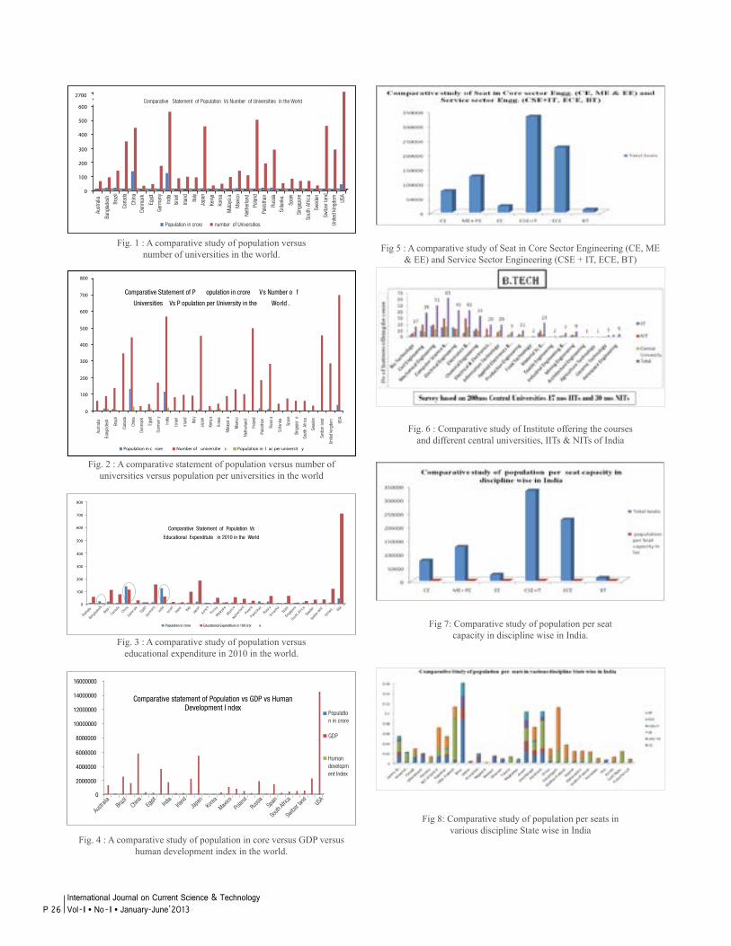
Fig. 1 : A comparative study of population versusnumber of universities in the world.
Fig. 2 : A comparative statement of population versus number of universities versus population per universities in the world
Fig. 3 : A comparative study of population versuseducational expenditure in 2010 in the world.
Fig. 4 : A comparative study of population in core versus GDP versus human development index in the world.
Fig 5 : A comparative study of Seat in Core Sector Engineering (CE, ME & EE) and Service Sector Engineering (CSE + IT, ECE, BT)
Fig. 6 : Comparative study of Institute offering the coursesand different central universities, IITs & NITs of India
Fig 7: Comparative study of population per seatcapacity in discipline wise in India.
Fig 8: Comparative study of population per seats invarious discipline State wise in India
Population in crore number of Universities
Aust
ralia
Bang
lade
sh
Braz
il
Cana
da
Chin
a
Denm
ark
Egyp
t
Garm
any
India
Isra
el
Irlan
d
Italy
Japa
n
Keny
a
Kore
a
Mal
aysi
a
Max
ico
Neth
erla
nd
Pola
nd
Paki
stha
n
Russ
ia
Srila
nka
Spain
Sing
apor
e
Sout
h Af
rica
Swed
en
Switz
er la
nd
Unite
d ki
ngdo
m
USA
600
500
400
300
200
100
0
2700Comparative Statement of Population Vs Number of Universities in the World
Population in l ac per universit yNumber of universitie sPopulation in c rore
Comparative Statement of P opulation in crore Vs Number o f
Universities Vs P opulation per University in the World .
800
700
600
500
400
300
200
100
0
Aust
ralia
Ban
glad
esh
Braz
il
Cana
da
Chin
a
Den
mar
k
Egyp
t
Gar
man
y
Indi
a
Isra
el
Irlan
d
Italy
Japa
n
Keny
a
Kore
a
Mal
aysi
a
Max
ico
Neth
erla
nd
Pola
nd
Paki
stha
n
Russ
ia
Srila
nka
Spai
n
Sing
apor
e
Sout
h Af
rica
Swed
en
Switz
er la
nd
Unite
d ki
ngdo
m USA
Population in crore Educational Expenditure in 100 cror e
Comparative Statement of Population Vs
Educational Expenditute in 2010 in the World
800
700
600
500
400
300
200
100
0
Austral
ia
Bangla
desh
Brazi
lCan
ada
China
Denm
arkEg
ypt
Garm
any
India
Israe
lIrla
nd Italy
Japan
Keny
a
Korea
Malays
i aM
axico
Nethe
rland
Polan
dPak
is tha
n
Russi
a
Sri lan
kaSp
ainSing
apore
South
Afri
caSw
eden
Switz
er lan
dUnit
ed... USA
Humandevelopment Index
Comparative statement of Population vs GDP vs HumanDevelopment I ndex
16000000
14000000
12000000
10000000
8000000
6000000
4000000
2000000
0
GDP
Population in crore
Austra
liaBraz
il
China
Egypt Ind
ia
Irland
Japa
nKore
a
Maxico
Polan
d
Russi
aSp
ain
South
Afric
a
Switze
r land US
A
P 26International Journal on Current Science & Technology Vol - I l No- I l January-June’2013
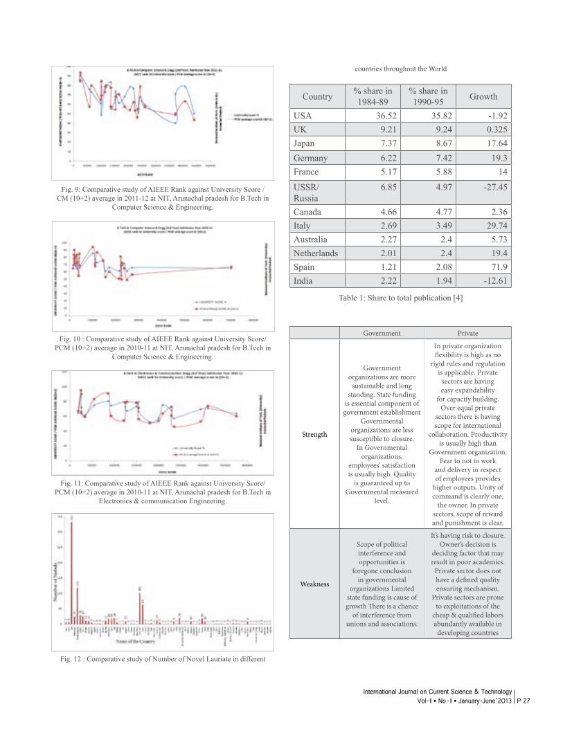
Fig. 9: Comparative study of AIEEE Rank against University Score / CM (10+2) average in 2011-12 at NIT, Arunachal pradesh for B.Tech in
Computer Science & Engineering.
Fig. 10 : Comparative study of AIEEE Rank against University Score/PCM (10+2) average in 2010-11 at NIT, Arunachal pradesh for B.Tech in
Computer Science & Engineering.
Fig. 11: Comparative study of AIEEE Rank against University Score/PCM (10+2) average in 2010-11 at NIT, Arunachal pradesh for B.Tech in
Electronics & communication Engineering.
Fig. 12 : Comparative study of Number of Novel Lauriate in different
countries throughout the World
Country % share in 1984-89
% share in 1990-95 Growth
USA 36.52 35.82 -1.92UK 9.21 9.24 0.325Japan 7.37 8.67 17.64Germany 6.22 7.42 19.3France 5.17 5.88 14
USSR/Russia
6.85 4.97 -27.45
Canada 4.66 4.77 2.36Italy 2.69 3.49 29.74Australia 2.27 2.4 5.73Netherlands 2.01 2.4 19.4Spain 1.21 2.08 71.9India 2.22 1.94 -12.61
Table 1: Share to total publication [4]
Government Private
Strength
Government organizations are more
sustainable and long standing. State funding
is essential component of government establishment
Governmental organizations are less susceptible to closure.
In Governmental organizations,
employees’ satisfaction is usually high. Quality
is guaranteed up to Governmental measured
level.
In private organization flexibility is high as no
rigid rules and regulation is applicable. Private
sectors are having easy expandability
for capacity building. Over equal private
sectors there is having scope for international
collaboration. Productivity is usually high than
Government organization. Fear to not to work
and delivery in respect of employees provides
higher outputs. Unity of command is clearly one,
the owner. In private sectors, scope of reward and punishment is clear.
Weakness
Scope of political interference and opportunities is
foregone conclusion in governmental
organizations Limited state funding is cause of growth There is a chance
of interference from unions and associations.
It’s having risk to closure. Owner’s decision is
deciding factor that may result in poor academics.
Private sector does not have a defined quality ensuring mechanism.
Private sectors are prone to exploitations of the
cheap & qualified labors abundantly available in developing countries
P 27International Journal on Current Science & Technology
Vol - I l No- I l January-June’2013
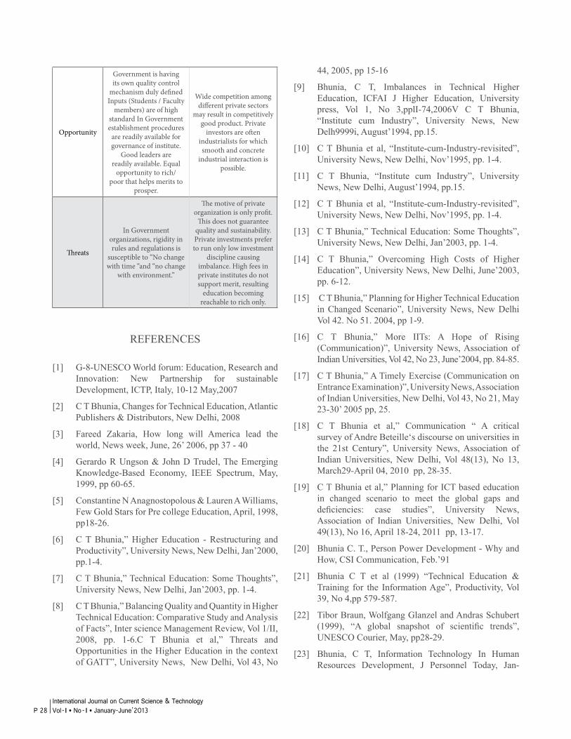
Opportunity
Government is having its own quality control
mechanism duly defined Inputs (Students / Faculty
members) are of high standard In Government establishment procedures
are readily available for governance of institute.
Good leaders are readily available. Equal
opportunity to rich/poor that helps merits to
prosper.
Wide competition among different private sectors
may result in competitively good product. Private
investors are often industrialists for which smooth and concrete
industrial interaction is possible.
Threats
In Government organizations, rigidity in rules and regulations is
susceptible to “No change with time “and “no change
with environment.”
The motive of private organization is only profit.
This does not guarantee quality and sustainability. Private investments prefer to run only low investment
discipline causing imbalance. High fees in private institutes do not support merit, resulting
education becoming reachable to rich only.
REFERENCES
[1] G-8-UNESCO World forum: Education, Research and Innovation: New Partnership for sustainable Development, ICTP, Italy, 10-12 May,2007
[2] C T Bhunia, Changes for Technical Education, Atlantic Publishers & Distributors, New Delhi, 2008
[3] Fareed Zakaria, How long will America lead the world, News week, June, 26’ 2006, pp 37 - 40
[4] Gerardo R Ungson & John D Trudel, The Emerging Knowledge-Based Economy, IEEE Spectrum, May, 1999, pp 60-65.
[5] Constantine N Anagnostopolous & Lauren A Williams, Few Gold Stars for Pre college Education, April, 1998, pp18-26.
[6] C T Bhunia,” Higher Education - Restructuring and Productivity”, University News, New Delhi, Jan’2000, pp.1-4.
[7] C T Bhunia,” Technical Education: Some Thoughts”, University News, New Delhi, Jan’2003, pp. 1-4.
[8] C T Bhunia,” Balancing Quality and Quantity in Higher Technical Education: Comparative Study and Analysis of Facts”, Inter science Management Review, Vol 1/II, 2008, pp. 1-6.C T Bhunia et al,” Threats and Opportunities in the Higher Education in the context of GATT”, University News, New Delhi, Vol 43, No
44, 2005, pp 15-16
[9] Bhunia, C T, Imbalances in Technical Higher Education, ICFAI J Higher Education, University press, Vol 1, No 3,pplI-74,2006V C T Bhunia, “Institute cum Industry”, University News, New Delh9999i, August’1994, pp.15.
[10] C T Bhunia et al, “Institute-cum-Industry-revisited”, University News, New Delhi, Nov’1995, pp. 1-4.
[11] C T Bhunia, “Institute cum Industry”, University News, New Delhi, August’1994, pp.15.
[12] C T Bhunia et al, “Institute-cum-Industry-revisited”, University News, New Delhi, Nov’1995, pp. 1-4.
[13] C T Bhunia,” Technical Education: Some Thoughts”, University News, New Delhi, Jan’2003, pp. 1-4.
[14] C T Bhunia,” Overcoming High Costs of Higher Education”, University News, New Delhi, June’2003, pp. 6-12.
[15] C T Bhunia,” Planning for Higher Technical Education in Changed Scenario”, University News, New Delhi Vol 42. No 51. 2004, pp 1-9.
[16] C T Bhunia,” More IITs: A Hope of Rising (Communication)”, University News, Association of Indian Universities, Vol 42, No 23, June’2004, pp. 84-85.
[17] C T Bhunia,” A Timely Exercise (Communication on Entrance Examination)”, University News, Association of Indian Universities, New Delhi, Vol 43, No 21, May 23-30’ 2005 pp, 25.
[18] C T Bhunia et al,” Communication “ A critical survey of Andre Beteille‘s discourse on universities in the 21st Century”, University News, Association of Indian Universities, New Delhi, Vol 48(13), No 13, March29-April 04, 2010 pp, 28-35.
[19] C T Bhunia et al,” Planning for ICT based education in changed scenario to meet the global gaps and deficiencies: case studies”, University News, Association of Indian Universities, New Delhi, Vol 49(13), No 16, April 18-24, 2011 pp, 13-17.
[20] Bhunia C. T., Person Power Development - Why and How, CSI Communication, Feb.’91
[21] Bhunia C T et al (1999) “Technical Education & Training for the Information Age”, Productivity, Vol 39, No 4,pp 579-587.
[22] Tibor Braun, Wolfgang Glanzel and Andras Schubert (1999), “A global snapshot of scientific trends”, UNESCO Courier, May, pp28-29.
[23] Bhunia, C T, Information Technology In Human Resources Development, J Personnel Today, Jan-
P 28International Journal on Current Science & Technology Vol - I l No- I l January-June’2013

March’ 1998,pp 43-47
[24] Bhunia C T, Basic Investigation on E-learning, CSI Communication, March’2005 Mumbai, ppl7-21
[25] G-8-UNESCO World forum: Education, Research and Innovation: New Partnership for sustainable Development, ICTP, Italy, 10-12 May,2007
[26] http ://www2.mea.org/he/ future/market.html
[27] Ritz J M M Dr ir, Scenario for Higher Education, 2020, Keynote Address at OECD Ministerial Meeting, June 27h ,2006Athens, Greece
[28] David Collis, Book : When Industries Change: Scenarios for Higher Education, Ch 3.
P 29International Journal on Current Science & Technology
Vol - I l No- I l January-June’2013

P 30International Journal on Current Science & Technology Vol - I l No- I l January-June’2013
IMBALANCE IN TECHNICAL EDUCATION-REGIONAL
Bikash Sah, Nupur, Santosh Shukla, Krishna Kumar
Students, B.Tech Course, Electrical and Electronics EngineeringNational Institute of Technology, Arunachal Pradesh
Yupia, Papum Pare [email protected], [email protected], [email protected]
ABSTRACT
A country stands on its intellectual population and for the development of intellectuals; role of education is at the highest priority. Further the role of education in facilitating the economic progress has already been identified all over the world. Our nation has made a noticeable progress in the field of higher and technical education. This paper analyses the imbalances created on the basis of region and its hard impact on the economy and growth of our country. It also analyses the impact on quality of education system introduced due to regional imbalance and suggest some changes that can be implemented to improve the present scenario.
Keywords : India, Economy, Technical education system, UGC, Institutions, Regional Imbalance, Quality.
I. NTRODUCTION
The policy of LPG (Liberalization, privatization and globalization) has changed the scenario of present context. It has been found that the economic growth is directly influenced by the quality of technical education that a country imparts. Various sources like the World Bank and World Economics Association have shown that higher education enrolment is a leading indicator of economic growth. [1]If the number of students enrolled and educated by universities of a country increases rapidly, it can be found that the country thrives in economic growth in the decade to follow. This already has been proved in the case of countries like Japan and Korea. [2]Technology has become an important parameter that determines the growth of the country (economically, socially and politically). Imparting education to the citizens doesn’t actually mean the country is developing, but that is quality whichtruly determines the worthiness of education imparted.Consider for instance the context of globalization of economy, underdeveloped and the developing countries need to compete with the developed and technologically advanced world that has technically sound human resourceand other
resourceto enhance their productivity. Time has proven the importance of quality in technical education for developing a country.India, being a developing country needs to focus on its ways of imparting technical education. There is a dire need of an economy, created by intellectual capital and run by the knowledge and wisdom. This intellectual capital will play an important role in future enterprises and thus technical education has become imperative for the country.The rapid increases in establishment of institutions may have introduced a greater compromise with the quality. An imbalance has emerged in the technical education scenario. This imbalance is not in a specific field but has spread out like an epidemic in all the fields right from the opening of an institution till its complete setup and healthy functioning.It is said that “India” our country has been proceeding ahead remarkably in the field of technical education for the last two decades, but is it really true? And have we really been able to overcome the shortcomings, challenges and able to reap the opportunities successfully?We can clearly find an imbalance on the basis of region, quantity, ownership, course, intellect, physical resources and training process in our country.
Technical education in India is imparted in three different levels:
1. ITI(Industrial training Institute) also known asATI(Advanced Training Institute)
2. Polytechnics (Diploma institute)
3. B-Tech or higher college/university. [3]
Theplans made by the governmentvirtually need appreciation. For example the five year plans of University Grants Commission (UGC), a statutory organisation set up by Union Government, to look over universities and colleges at higher education in India,but don’t go deep into the ground problems for finding solutions. We have a number of higher and technical institutions in India but they are not distributed in a uniform manner rather are concentrated in some of the
P 31International Journal on Current Science & Technology
Vol - I l No- I l January-June’2013
particular states or regions only. This give rise to one of the greatest form of imbalance called as “Regional Imbalance” which has been explained in the forthcoming paragraphs with its impact in the Quality of education provided.
II. REGIONAL IMBALANCE
The most roaring form of imbalance in our country is Regional Imbalance. LPG (Liberalization, Privatization, and Globalization) are the causes for the introduction of this imbalance.
Institutions were set-up but not in the productive manner. Every investor looked at these establishments in their own way and focussed mainly on the profit in running their establishment. This led to a sudden appearance of huge number of institutionsin populated areas of the country like the central India and south India. A sense of awareness came among the common people regarding the importance of technical education. This privatization of educational process couldn’t fullybenefit some of the Indian states that urgently needed to have technically sound population. Even within the states, this imbalance had developed prominently. The regions which demand privatization are more advanced than the regions which gives importance to agriculture or don’t support LPG. [4]
Indian UGC fairly setup 5- Year plans which always says “Considerable challenges remain” i.e. it fails to execute some plans while the other countries don’t set-up such ambitious plans.
Maharashtra is considered as one of the most advanced state in providing technical education. It has 44 universities, 470 engineering colleges and 182 polytechnic institutions. The Maharashtra State Board of Technical Education handles all the proceeding of every single technical college; on the other hand we have our North-Eastern states which have scanty technical institutes. Arunachal Pradesh for instancehas a total number of 2 universities, two engineering college and two polytechnic colleges. Higher and technical institutions’ are in the ratio of 22:1, 235:1 and 91:2 respectively. An unbelievable difference can be catered among not only these two states but among other states as well. [5]
The imbalance is not only among the states but also within the state itself. For state with larger area like Uttar Pradesh, majority of the institutions are settled in areas of Noida, Allahabad, Lucknow, Banaras and other urban areas. The rest parts of the state lack the facility of proper higher education in their footsteps. There are intra-state imbalances with Pareto’s Law of misdistribution leading to ‘vital few and ‘ ignored many regions where these new colleges have emerged.
The imbalance has influenced other important topics as well including the “Quality”, without which the aim to develop a skilful and technically advanced India fails. The quality of education imparted is based on various facilities we give, like intellectuals, state of the art Laboratories etc. A small example of an intellectual at base level is Lab-Technician. The appointment of a lab technician in an institute is an important activity. The technician should have the required skills to guide his/her students to let them understand topics and present as a practically feasible topic infront of the student. The lack of motivation and commitment among the intellectual is another negative prospect of this imbalance.It has been found that more than 80% of the institutes affiliated to AICTE are simple B-Tech with inadequate academic performance. Lacks of good management by the authority has diverted the students in a different way instead of encouraging them to move towards Research and Development(R&D). Foreign universities have a much higher ratio of students pursuing higher education after B-Tech as compared to India. The number of Ph.D. or M-Tech thesis and research papers published by Indian universities is very less as compared to other foreign universities. These allareas are a matter of concern as per the qualitative expansion of the Indian Technical Education.
With such a prevailing condition, still many investors are continuing to invest. Education is being considered a business by many people.
Another important point to be focussed is “Are Indian universities able to provide the education in a proper way? Is it meant or accessible to the common masses?”
We have IIT’s and IIM’s as our premier institutes on which we are proud, but these fail to impart education to masses. These institutes cover less than 10% of the whole mass pursuing higher education. Of these 42% only remain in India and other go abroad for future prospects. A complete brain drain is seen while other countries have taken various steps to stop this.Only 10,000 out of 12 crore strong university age population stand to support the country for its development. This creates an absence of intellectual population in India. Non availability of experienced faculty can be seen in most of the institutesin India. If one compares the statistics of institutes, he/she will find maximum new scholars who have just completed their post-graduate or Ph.D. As per the data collected from Uttar Pradesh (one of the states with highest number of technical institute’s) 80% of the faculty are fresh graduates ofearly twenties and 10-15% is from past 60 years mostly retired professors with an absence of middle cadre.[6]
The above quality situations are well known to every citizen of the nation including our own selected representatives, to whom we call our leaders.
P 32International Journal on Current Science & Technology Vol - I l No- I l January-June’2013
Dr.Manmohan Singh’s once quoted the following words:
“Our university system is, in many parts, in a state of disrepair...In almost half the districts in the country, higher education enrolments are abysmally low, almost two-third of our universities and 90 per cent of our colleges are rated as below average on quality parameters... I am concerned that in many states university appointments, including that of vice-chancellors, have been politicised and have become subject to caste and communal considerations, there are complaints of favouritism and corruption.” [7]
A crystal clear imbalance is visible to all the citizens of the nation. Imbalance is ruining the scenario all over. The imbalance is ruining the present era of competition among nations in all the fields.
On one hand government makes plan and introduces new institution to satisfy the need of higher technical education in India and on the other hand the government forgets the remaining perspective affecting the quality of education imparted. The present trend of information technology and economics has reduced the whole world into a small village called “A Global Village”. The communication gap has been reduced everywhere. [8]
Swami Vivekananda, one of the greatest saints of India once said “I need 40 lions (youths) to transform Bharat to a knowledge superpower”. Our nation indeed has a real potential to evolve as the knowledge superpower. It’s time to spread our potential in different fields rather than confining to a particular field. The ultimate patience to wait for the results of various plans have to be broken and every single step moved forward should focus on the positive result and the best should be only implemented.
Needs of globally expert and competent skilled people can be seen everywhere. A standard education system should be developed all over India to remove the imbalance andfocus on quality. The quantity increases the number of technically skilled citizens in a nation but they lack quality. On the whole we will have a lot of unemployed people all around who can’t be allowed to work because of the lack of perfectness a skilful person should have.
The programmes run by government of India for reducing the regional imbalance by maintaining quality of education provided should be made more effective. These programmes shouldnot be limited to any particular university or any institution; instead a common step should be taken by all the working agencies in this field.
TEQIP (Technical education quality improvement programme) run by the government of India should be made more effective in all the institution of country. This programme aim to enhance existing capabilities of the institution to become dynamic, demand drives, quality consciousness, efficient and forward looking responsive to rapid economic and technological developments occurring both at national and international levels. The most important thing of all the institutes on the basis of priority and the allotment of financial help called funds by the Indian government. [9]
The All India council of Technical Education have taken the following steps to reduce the imbalance:
1. Allowed a second shift of engineering colleges in existing engineering colleges only in those States where the number of seats available in engineering colleges per lakh of population is less than all India average.
2. For a balanced growth of various streams of education in Engineering & Technology, the Council had adopted a policy to allow establishment of new Engineering Institutions with at least three conventional branches as a mandatory requirement in the States where the number of seats available in engineering colleges per lakh of population in more than all India average, whereas in the States where the number of seats available in engineering colleges per lakh of population is less than the all India average, no such restriction is applicable.
3. The Council has permitted the possession of total land area in three adjacent pieces specifically in North Eastern States and hilly areas for setting up new technical institutions. [10]
III. CONCLUSION
“INTROSPECTION” The standards of education must not be limited to only a few number of institutions like IIT’s, IIMs, NIT’s and some of the renowned institution rather a measure of equality should be given to all the institution(let it be technical or any other field). [11]
The politics must not be mixed with the education system. ‘A Common way out’ thinking should be introduced all over the nation to maintain a balance and quality. This common way is based on the Public Private Partnership concept. It is understood that some of the place have advantage and they attract more investors but what about the remaining places. The remaining places can have some government aided
P 33International Journal on Current Science & Technology
Vol - I l No- I l January-June’2013
initiatives or Public Private Partnerships. The state can offer packages to private academic investors for development of model technical institutes in different district or regions. This will improve and induce a healthy concept of competition among all the institution and the wish of students to pursue higher education from a well-established institution can be met.
Before starting an institution, other demands should be fulfilled like the required resources that need to be catered. The approval from AICTE and other councils for recognition of an institution should be done in general public perspective of reducing the demand of good professional rather than a selfish perspective or regional basis. This general public or patriotic thinking will stop all those private investors to work upon who consider education as a business.
The focus shouldn’t be only in the organised sector but the focus should spread over the unorganised sector as well. The traditional education techniques should be incorporated and evolved with the developing modern and technological system.
There is a need to update and train the present faculties as per the recent advancement i.e. more faculty development programme should be conducted by government agencies in co-operation with some private partnership.
The need to understand the importance of encompassing government, public sector, private sector, research and academic institution consistent with the industrial, technological and economic future of our country.
Due to rapid growth of industries and economic growth, technical education have been developing to its leaps and bound in India but regional imbalance is still prevailing everywhere. Recent development in different fields like space, nuclear, computer and IT have given recognition all over the world. As the technical education determines the economic growth, thus it’s necessary to remove theregional imbalance and improve the quality of education imparted.
REFERENCES
[1] Bhunia C.T., Changes in Technical Education, Atlantic publishers and distributers (P) ltd.
[2] Vrat, Prem, Impart Quality in Technical Education, SME World, Dec 2010; Avera H William”The Economic Times”.
[3] Prof Nayak D.K.,ProfPatilMohite T.V., “Impact of globalization & it revolution on technical education”.
[4] Saha Samir, GhoshSamita,”Engineering education in India: Past, Present and Future”, Propagation, A journal of science Communication, Vol: 2, No: 2, July, 2011
[5] http://apdhte.nic.in/colleges.htm ;http://www. w o r l d c o l l e g e s . i n f o / M a h a r a s h t r a / MaharashtraCollege s.php
[6] Vrat, Prem, “Role of Technical Education in Emerging Indian Society: Opportunities and Challenges” RITES Journal, July 2009.
[7] “PM’s address at the 150th Anniversary Function of UniversityofMumbai”. http://pmindia.nic.in/ speech/content.asp?id=555
[8] Dr. Pant R.M. “Technical Education in North Eastern India: Problems and prospects”,IPEDR vol.12 (2011) © (2011).
[9] Govt. of India ”Project Implementation Plan on TEQIP” MHRD, August 2002.
[10] Press Information Bureau “Technical Education Imbalance in States”, February 3, 2013.
[11] Govt. of India,“Report of the working group on technical education for the XII five year plan”, September 2011.
P 34International Journal on Current Science & Technology Vol - I l No- I l January-June’2013
A COMPARATIVE STUDY OF FUNGAL DISEASES OF FRENCH BEAN (PHASEOLUS VULGARIS.L)
IN ORGANIC AND CONVENTIONAL FARMING SYSTEM
G.K.N.Chhetry
Department of Life Sciences Manipur University ,Canchipur ,Imphal,India,795003
H.C.Mangang
Department of Life Sciences Manipur University ,Canchipur ,Imphal,India,795003
ABSTRACT
French bean is a favorite vegetable to most of the households of the north east people including Manipur, where the crop is grown mostly in most homestead gardens for home consumption. Organic farming and conventional farming are two main farming practices vying for their acceptance in sustainable agriculture and feed the ever increasing human population with limited land resources. Organic farming is usually perceived as low yield but environment friendly while conventional farming as more productive but with huge input demand and hazardous environmental impact. In developing countries where there is still lack of modern agrochemicals, hence indigenous farmers relied on traditional agricultural practices which are organic by default. North east India is no exception to this and the organic mode of farming is prevalent in most of the places particularly hills of the region. Apart fromyield aspects, it is of interest to study the diseaseaspects which is a serious concern in the organic farming system. There are references about the effect of soil amendments on disease development especially of soil borne diseases in the organic fields, yet comparative details of the disease parameters in the two farming modes have not been reported from the region. As the disease parameters are constrains to yield, estimation of disease parameters such aspercent disease incidence (DI %), Percent disease Severity (DS %), Area Under Disease Progress Curve (AUDPC), and Apparent rate of infection (r) are considered important. As such data pertaining to these parameters were obtained and thepooled data was analyzed to test the null hypothesis that there is no difference between the two treatments in disease development .Study revealed that the application of Farm Yard Manure ( FYM) , the most widely used manure in organic farming system,reduced the AUDPC of four foliar fungal diseases of French bean as compared to conventional system where synthetic fertilizers were added. DI% of two pathogen causing root rots and a fruit rot of French bean wasalso foundrelatively lower in organic plots.Statistical analysis rejected the null hypothesis in favour of alternate hypothesis which means significant difference of disease development of French bean in two different farming systems
.The difference may be attributed to organic amendments of soil:- a sustainable mode of crop protection in organic farming system.
Keywords: organic farming, conventional farming, French bean, AUDPC,infection rate, soil amendment, FYM, Manipur
I. NTRODUCTION
French bean is a popular vegetable recipe for people of north east Indiaincluding Manipurwhere it is grown in most household gardens as favorite vegetable almost throughout the year. String less bean variety was preferred more compared to other varieties in Manipur. This crop is grown mainly in the organic garden environment for domestic consumption in the North east. In contrast, cultivation of crops in commercial scale is mostly done in non organic mode i.e. in conventional synthetic fertilizer based farming. A thorough study of fungal disease development in the organic farming system is expected to help in proper understanding of the fungal pathology of bean and its management in the organic farming system. Further, a comparative study between the two modes of farming namely organic and conventional may enable us in understanding the pros and cons of organic farming system with respect to fungal disease development of this crop in particular. This would enhance crop protection strategies in organic environment. For this, field trials were conducted for three consecutive years (2008-2011) in organic gardens where farmers practice organic mode by tradition. Disease parameters were recorded at weekly intervals and the pooled data were analyzed statistically to test the hypothesis that the observed disease parameters between the two farming systems were the same. The disease parameters under study includes percent disease incidence (DI %), Percent disease Severity (DS %), Area under disease progress curve (AUDPC), and Apparent rate of infection (r)
II. MATERIALS AND METHODS Seed procurementBean varieties commonly cultivated by the local people were selected. Three varieties which were phenotypically distinct,
P 35International Journal on Current Science & Technology
Vol - I l No- I l January-June’2013
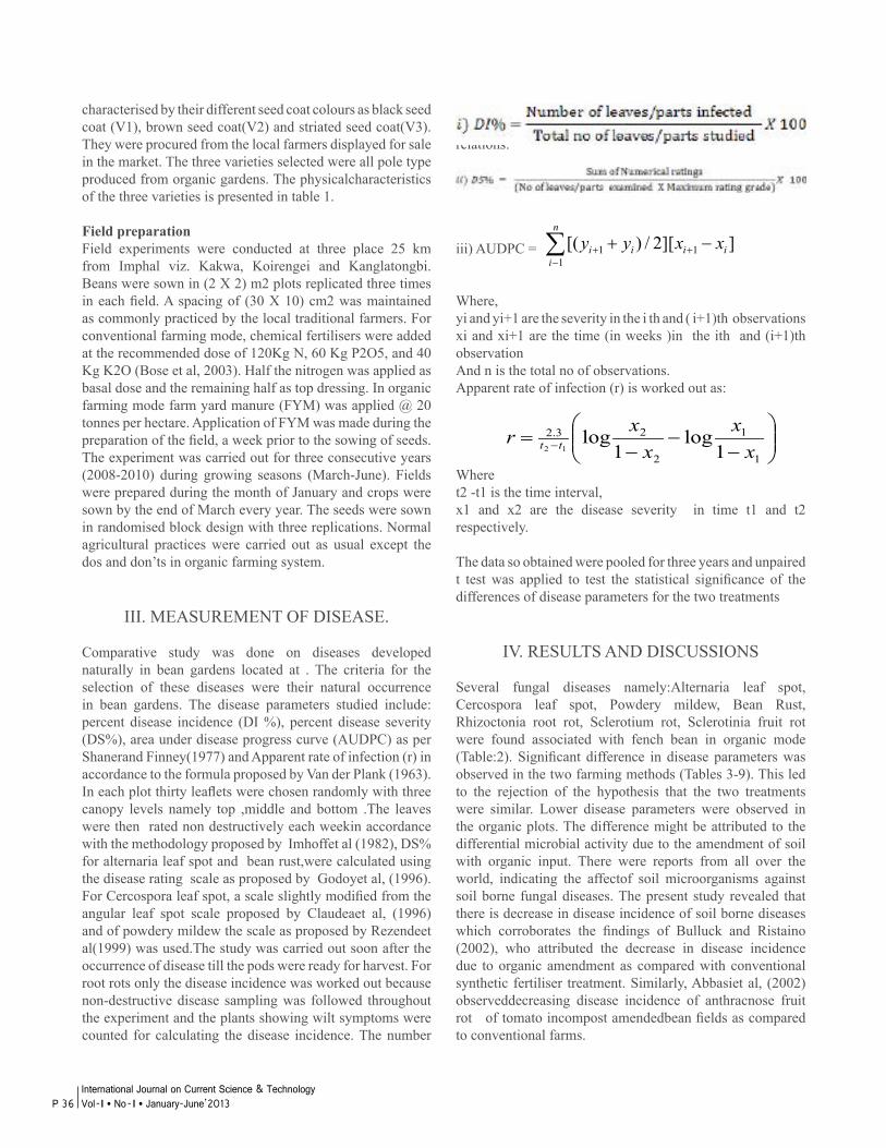
characterised by their different seed coat colours as black seed coat (V1), brown seed coat(V2) and striated seed coat(V3). They were procured from the local farmers displayed for sale in the market. The three varieties selected were all pole type produced from organic gardens. The physicalcharacteristics of the three varieties is presented in table 1.
Field preparationField experiments were conducted at three place 25 km from Imphal viz. Kakwa, Koirengei and Kanglatongbi. Beans were sown in (2 X 2) m2 plots replicated three times in each field. A spacing of (30 X 10) cm2 was maintained as commonly practiced by the local traditional farmers. For conventional farming mode, chemical fertilisers were added at the recommended dose of 120Kg N, 60 Kg P2O5, and 40 Kg K2O (Bose et al, 2003). Half the nitrogen was applied as basal dose and the remaining half as top dressing. In organic farming mode farm yard manure (FYM) was applied @ 20 tonnes per hectare. Application of FYM was made during the preparation of the field, a week prior to the sowing of seeds. The experiment was carried out for three consecutive years (2008-2010) during growing seasons (March-June). Fields were prepared during the month of January and crops were sown by the end of March every year. The seeds were sown in randomised block design with three replications. Normal agricultural practices were carried out as usual except the dos and don’ts in organic farming system.
III. MEASUREMENT OF DISEASE.
Comparative study was done on diseases developed naturally in bean gardens located at . The criteria for the selection of these diseases were their natural occurrence in bean gardens. The disease parameters studied include: percent disease incidence (DI %), percent disease severity (DS%), area under disease progress curve (AUDPC) as per Shanerand Finney(1977) and Apparent rate of infection (r) in accordance to the formula proposed by Van der Plank (1963). In each plot thirty leaflets were chosen randomly with three canopy levels namely top ,middle and bottom .The leaves were then rated non destructively each weekin accordance with the methodology proposed by Imhoffet al (1982), DS% for alternaria leaf spot and bean rust,were calculated using the disease rating scale as proposed by Godoyet al, (1996). For Cercospora leaf spot, a scale slightly modified from the angular leaf spot scale proposed by Claudeaet al, (1996) and of powdery mildew the scale as proposed by Rezendeet al(1999) was used.The study was carried out soon after the occurrence of disease till the pods were ready for harvest. For root rots only the disease incidence was worked out because non-destructive disease sampling was followed throughout the experiment and the plants showing wilt symptoms were counted for calculating the disease incidence. The number
of infected pods was recorded for pod rot disease incidence. The disease parameters were worked out as per the following relations:
iii) AUDPC =
Where,yi and yi+1 are the severity in the i th and ( i+1)th observationsxi and xi+1 are the time (in weeks )in the ith and (i+1)th observation And n is the total no of observations.Apparent rate of infection (r) is worked out as:
Where t2 -t1 is the time interval,x1 and x2 are the disease severity in time t1 and t2 respectively.
The data so obtained were pooled for three years and unpaired t test was applied to test the statistical significance of the differences of disease parameters for the two treatments
IV. RESULTS AND DISCUSSIONS
Several fungal diseases namely:Alternaria leaf spot, Cercospora leaf spot, Powdery mildew, Bean Rust, Rhizoctonia root rot, Sclerotium rot, Sclerotinia fruit rot were found associated with fench bean in organic mode (Table:2). Significant difference in disease parameters was observed in the two farming methods (Tables 3-9). This led to the rejection of the hypothesis that the two treatments were similar. Lower disease parameters were observed in the organic plots. The difference might be attributed to the differential microbial activity due to the amendment of soil with organic input. There were reports from all over the world, indicating the affectof soil microorganisms against soil borne fungal diseases. The present study revealed that there is decrease in disease incidence of soil borne diseases which corroborates the findings of Bulluck and Ristaino (2002), who attributed the decrease in disease incidence due to organic amendment as compared with conventional synthetic fertiliser treatment. Similarly, Abbasiet al, (2002) observeddecreasing disease incidence of anthracnose fruit rot of tomato incompost amendedbean fields as compared to conventional farms.
]][2/)[( 1
11 iii
n
ii xxyy −+ +
−+∑
−
−−
= −1
1
2
23.2
1log
1log
12 xx
xxr tt
P 36International Journal on Current Science & Technology Vol - I l No- I l January-June’2013
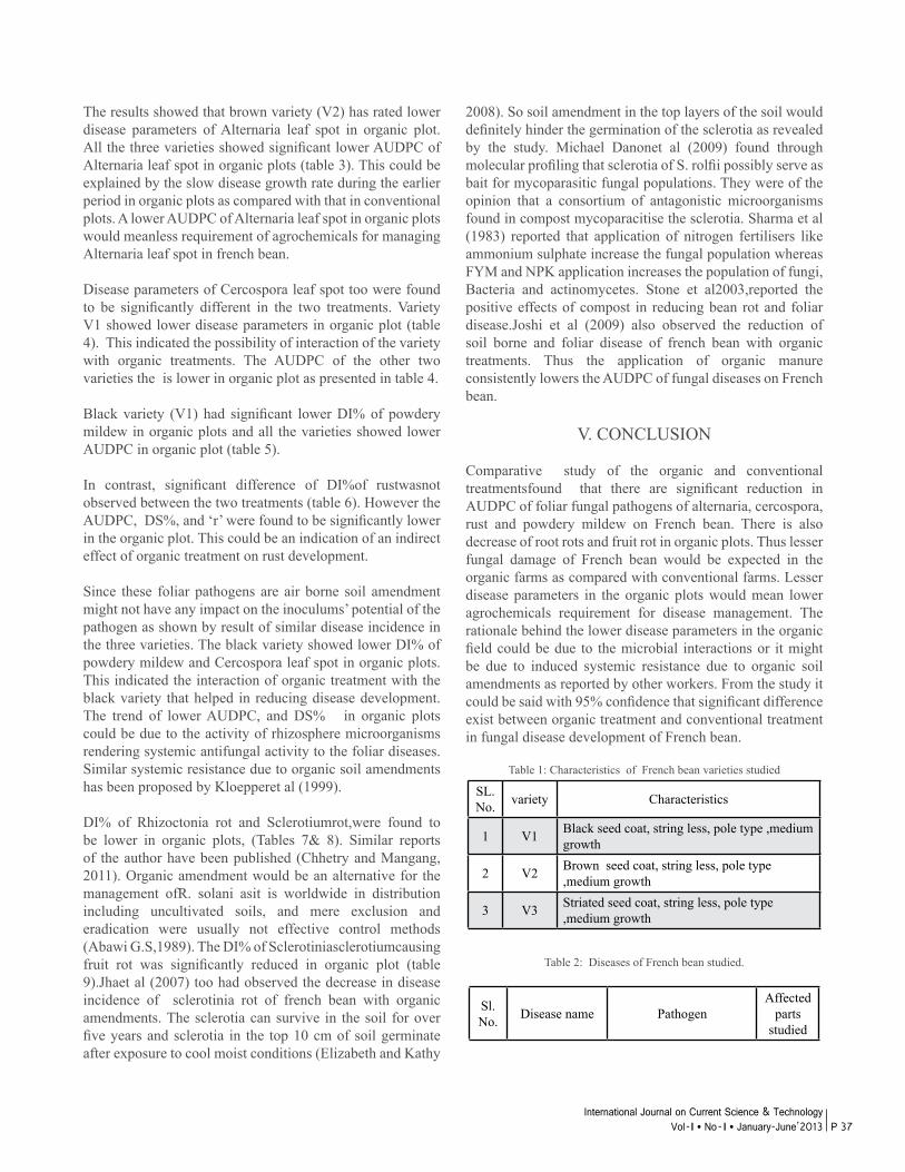
The results showed that brown variety (V2) has rated lower disease parameters of Alternaria leaf spot in organic plot. All the three varieties showed significant lower AUDPC of Alternaria leaf spot in organic plots (table 3). This could be explained by the slow disease growth rate during the earlier period in organic plots as compared with that in conventional plots. A lower AUDPC of Alternaria leaf spot in organic plots would meanless requirement of agrochemicals for managing Alternaria leaf spot in french bean.
Disease parameters of Cercospora leaf spot too were found to be significantly different in the two treatments. Variety V1 showed lower disease parameters in organic plot (table 4). This indicated the possibility of interaction of the variety with organic treatments. The AUDPC of the other two varieties the is lower in organic plot as presented in table 4.
Black variety (V1) had significant lower DI% of powdery mildew in organic plots and all the varieties showed lower AUDPC in organic plot (table 5).
In contrast, significant difference of DI%of rustwasnot observed between the two treatments (table 6). However the AUDPC, DS%, and ‘r’ were found to be significantly lower in the organic plot. This could be an indication of an indirect effect of organic treatment on rust development.
Since these foliar pathogens are air borne soil amendment might not have any impact on the inoculums’ potential of the pathogen as shown by result of similar disease incidence in the three varieties. The black variety showed lower DI% of powdery mildew and Cercospora leaf spot in organic plots. This indicated the interaction of organic treatment with the black variety that helped in reducing disease development. The trend of lower AUDPC, and DS% in organic plots could be due to the activity of rhizosphere microorganisms rendering systemic antifungal activity to the foliar diseases. Similar systemic resistance due to organic soil amendments has been proposed by Kloepperet al (1999).
DI% of Rhizoctonia rot and Sclerotiumrot,were found to be lower in organic plots, (Tables 7& 8). Similar reports of the author have been published (Chhetry and Mangang, 2011). Organic amendment would be an alternative for the management ofR. solani asit is worldwide in distribution including uncultivated soils, and mere exclusion and eradication were usually not effective control methods (Abawi G.S,1989). The DI% of Sclerotiniasclerotiumcausing fruit rot was significantly reduced in organic plot (table 9).Jhaet al (2007) too had observed the decrease in disease incidence of sclerotinia rot of french bean with organic amendments. The sclerotia can survive in the soil for over five years and sclerotia in the top 10 cm of soil germinate after exposure to cool moist conditions (Elizabeth and Kathy
2008). So soil amendment in the top layers of the soil would definitely hinder the germination of the sclerotia as revealed by the study. Michael Danonet al (2009) found through molecular profiling that sclerotia of S. rolfii possibly serve as bait for mycoparasitic fungal populations. They were of the opinion that a consortium of antagonistic microorganisms found in compost mycoparacitise the sclerotia. Sharma et al (1983) reported that application of nitrogen fertilisers like ammonium sulphate increase the fungal population whereas FYM and NPK application increases the population of fungi, Bacteria and actinomycetes. Stone et al2003,reported the positive effects of compost in reducing bean rot and foliar disease.Joshi et al (2009) also observed the reduction of soil borne and foliar disease of french bean with organic treatments. Thus the application of organic manure consistently lowers the AUDPC of fungal diseases on French bean.
V. CONCLUSION
Comparative study of the organic and conventional treatmentsfound that there are significant reduction in AUDPC of foliar fungal pathogens of alternaria, cercospora, rust and powdery mildew on French bean. There is also decrease of root rots and fruit rot in organic plots. Thus lesser fungal damage of French bean would be expected in the organic farms as compared with conventional farms. Lesser disease parameters in the organic plots would mean lower agrochemicals requirement for disease management. The rationale behind the lower disease parameters in the organic field could be due to the microbial interactions or it might be due to induced systemic resistance due to organic soil amendments as reported by other workers. From the study it could be said with 95% confidence that significant difference exist between organic treatment and conventional treatment in fungal disease development of French bean.
Table 1: Characteristics of French bean varieties studied
SL. No. variety Characteristics
1 V1 Black seed coat, string less, pole type ,medium growth
2 V2 Brown seed coat, string less, pole type ,medium growth
3 V3 Striated seed coat, string less, pole type ,medium growth
Table 2: Diseases of French bean studied.
Sl. No. Disease name Pathogen
Affected parts
studied
P 37International Journal on Current Science & Technology
Vol - I l No- I l January-June’2013

1 Alternaria leaf spot
Alternaria alternate leaves
2 Cercospora leaf spot
Cercosporacanescens leaves
3 Powdery mildew
Erisiphepolygoni leaves
4 Rust Uromycesappendiculatus leaves
5 Rhizoctonia root rot
Rhizoctoniasolani roots
6 Sclerotinia rot Sclerotiumrolfsii Roots
7 Sclerotinia fruit rot
Sclerotiniasclerotium pods
Table 3: Effect of organic and conventional treatment on Alternaria leaf spot.
Trea
tmen
ts
Year DI% DS% AUDPC r
V1
V2
V3
V1
V2
V3
V1
V2
V3
V1
V2
V3
Org
anic
08 60.1
3
60.1
1
60.0
1
18.6
7
16.4
5
17.5
4
25.3
4
26.4
6
25.1
2
0.13
0.11
0.07
09 55.2
6
41.2
4
63.0
0
18.4
8
16.6
6
18.2
6
25.0
7
25.9
8
25.6
7
0.13
0.09
0.09
10 59.3
8
50.5
4
55.7
6
19.9
8
17.0
7
18.4
7
25.5
7
25.7
7
25.8
9
0.12
0.09
0.09
mea
n
58.2
6
50.6
3
59.5
9
19.0
4
16.7
3
18.0
9
25.3
3
26.0
7
25.5
6
0.13
0.10
0.08
Con
vent
.
08 57.6
3
72.1
1
59.7
6
20.1
3
18.2
4
20.0
1
27.0
9
29.3
5
28.3
6
0.12
0.13
0.13
09 58.4
2
65.5
4
55.3
1
18.3
1
17.6
2
19.6
9
28.0
0
28.9
7
27.9
5
0.12
0.13
0.13
10 58.1
0
72.4
6
58.0
4
18.4
18.4
3
20.1
7
29.8
9
28.8
7
28.6
6
0.13
0.14
0.12
mea
n
58.0
5
70.0
4
57.7
0
18.9
5
18.1
0
19.9
6
28.3
3
29.0
6
28.3
2
0.12
0.13
0.13
‘t’ v
alue
0.13
3.29
*
0.76
0.13
4.49
*
5.92
*
3.58
*
11.9
2*
8.98
*
0.71
4.92
*
5.81
*
*significant at p<0.05
Table 4: Effect of organic and conventional treatmenton cercospora leaf spot
Table 5: Effect of organic and conventional treatment on powdery mildew
Trea
tmen
ts
year DI% DS% AUDPC r
V1
V2
V3
V1
V2
V3
V1
V2
V3
V1
V2
V3
Org
anic
08 35.2
6
38.3
6
38.8
7
9.41
10.1
1
9.48
20.1
2
21.1
2
20.2
3
0.07
0.08
0.06
09 34.1
8
29.3
2
32.7
5
9.12
9.16 9.4
20.3
4
20.5
6
21.0
1
0.1
0.1
0.07
10 30.3
7
30.2
4
39.2
6
8.43
7.14
8.52
21.0
1
20.3
4
20.4
5
0.09
0.11
0.06
mea
n
33.2
7
32.6
4
36.9
6
8.99 8.8
9.13
20.4
9
20.6
7
20.5
6
0.09 0.1
0.06
Con
vent
.
08 42.1
7
40.3
6
43.2
6
10.6
4
11.3
7
10.8
9
23.5
4
23.1
1
24.4
5
0.12
0.09
0.07
09 38.7
35.3
3
37.1
6
10.1
5
11.1
6
11.5
6
24.0
1
24.0
1
24.5
9
0.11 0.1
0.06
10 38.5
7
37.8
4
40.1
1
9.96
9.12
10.0
2
24.0
2
23.7
8
24 0.13
0.12
0.06
mea
n
39.8
1
37.8
4
40.1
8
10.2
5
10.5
5
10.8
2
23.8
6
23.6
3
24.3
5
0.12 0.1
0.06
‘t’ v
alue
3.45
*
1.61
1.17
3.57
*
1.54
3.12
*
10.8
2*
8.31
*
12.9
3*
3.16
*
0.53
0.01
Table 6: Effect of organic and conventional treatment on rust
Trea
tmen
ts
year DI% DS% AUDPC r
V1
V2
V3
V1
V2
V3
V1
V2
V3
V1
V2
V3
Org
anic
08 65.4
8
63.3
7
63.1
4
7.14
8.37
5.00
20.6
1
22.4
8
23.5
8
0.34
0.35
0.41
09 68.9
7
68.8
9
70.0
8
9.96
10.1
0
9.96
22.9
3
24.3
5
24.6
0
0.37
0.39
0.47
10 64.6
4
61.0
8
66.1
0
5.00
8.33
4.32
19.5
9
22.2
0
22.7
3
0.32
0.35
0.39
mea
n
66.7
0
64.4
5
66.4
4
7.37
8.93
6.43
21.0
4
23.0
1
23.6
4
0.34
0.36
0.42
P 38International Journal on Current Science & Technology Vol - I l No- I l January-June’2013
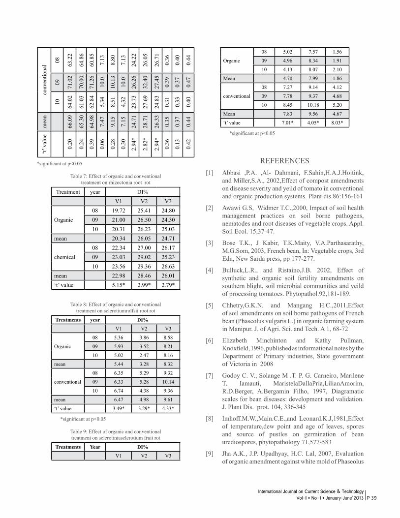
conv
entio
nal 08 63
.22
64.8
6
60.8
5
7.13
8.80
7.13
24.2
2
26.0
5
26.7
1
0.36
0.40
0.44
09 71.0
2
70.0
0
71.2
6
10.0
10.1
3
10.0
26.2
6
32.4
0
27.4
5
0.39
0.37
0.47
10 64.0
2
61.0
3
62.8
4
5.34
8.51
4.32
23.7
3
27.6
9
24.8
3
0.31
0.33
0.40
mea
n
66.0
9
65.3
0
64.9
8
7.47
9.15
7.15
24.7
1
28.7
1
26.3
3
0.35
0.37
0.44
‘t’ v
alue
0.20
0.24
0.39
0.06
0.28
0.30
2.94
*
2.82
*
2.94
*
0.36
0.13
0.42
*significant at p<0.05
Table 7: Effect of organic and conventionaltreatment on rhizoctonia root rot
Treatment year DI%V1 V2 V3
Organic 08 19.72 25.41 24.8009 21.00 26.50 24.3010 20.31 26.23 25.03
mean 20.34 26.05 24.71
chemical08 22.34 27.00 26.1709 23.03 29.02 25.2310 23.56 29.36 26.63
mean 22.98 28.46 26.01‘t’ value 5.15* 2.99* 2.79*
Table 8: Effect of organic and conventionaltreatment on sclerotiumrolfsii root rot
Treatments year DI%
V1 V2 V3
Organic
08 5.36 3.86 8.58
09 5.93 3.52 8.21
10 5.02 2.47 8.16
mean 5.44 3.28 8.32
conventional
08 6.35 5.29 9.32
09 6.33 5.28 10.14
10 6.74 4.38 9.36
mean 6.47 4.98 9.61
‘t’ value 3.49* 3.29* 4.33*
*significant at p<0.05
Table 9: Effect of organic and conventionaltreatment on sclerotiniasclerotium fruit rot
Treatments Year DI%
V1 V2 V3
Organic
08 5.02 7.57 1.56
09 4.96 8.34 1.91
10 4.13 8.07 2.10
Mean 4.70 7.99 1.86
conventional
08 7.27 9.14 4.12
09 7.78 9.37 4.68
10 8.45 10.18 5.20
Mean 7.83 9.56 4.67
‘t’ value 7.01* 4.05* 8.03*
*significant at p<0.05
REFERENCES[1] Abbasi ,P.A. ,Al- Dahmani, F.Sahin,H.A.J.Hoitink, and Miller,S.A., 2002,Effect of compost amendments on disease severity and yeild of tomato in conventional and organic production systems. Plant dis.86:156-161
[2] Awawi G.S, Widmer T.C.,2000, Impact of soil health management practices on soil borne pathogens, nematodes and root diseases of vegetable crops. Appl. Soil Ecol. 15,37-47.
[3] Bose T.K., J Kabir, T.K.Maity, V.A.Parthasarathy, M.G.Som, 2003, French bean, In: Vegetable crops, 3rd Edn, New Sarda press, pp 177-277.
[4] Bulluck,L.R., and Ristaino,J.B. 2002, Effect of synthetic and organic soil fertility amendments on southern blight, soil microbial communities and yeild of processing tomatoes. Phytopathol.92,181-189.
[5] Chhetry,G.K.N. and Mangang H.C.,2011,Effect of soil amendments on soil borne pathogens of French bean (Phaseolus vulgaris L.) in organic farming system in Manipur. J. of Agri. Sci. and Tech. A 1, 68-72
[6] Elizabeth Minchinton and Kathy Pullman, Knoxfield, 1996, published as informational notes by the Department of Primary industries, State government of Victoria in 2008
[7] Godoy C. V., Solange M .T. P. G. Carneiro, Marilene T. Iamauti, MaristelaDallaPria,LilianAmorim, R.D.Berger, A.Bergamin Filho, 1997, Diagramatic scales for bean diseases: development and validation. J. Plant Dis. prot. 104, 336-345
[8] Imhoff.M.W.,Main.C.E.,and Leonard.K.J,1981,Effect of temperature,dew point and age of leaves, spores and source of pustles on germination of bean urediospores, phytopathology 71,577-583
[9] Jha A.K., J.P. Upadhyay, H.C. Lal, 2007, Evaluation of organic amendment against white mold of Phaseolus
P 39International Journal on Current Science & Technology
Vol - I l No- I l January-June’2013
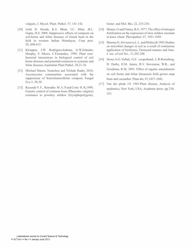
vulgaris, J. Mycol. Plant. Pathol. 37, 141-142.
[10] Joshi D. Hooda, K.S. Bhatt, J.C. Mina .B.L. Gupta, H.S. 2009, Suppressive effects of composts on soil-borne and foliar diseases of french bean in the field in western Indian Himalayas, Crop prot. 28, 608-615.
[11] Kloepper, J.W. Rodriguez-kabana, G.W.Zehnder, Murphy, E Sikora, C.Fernandez, 1999, Plant root- bacterial interactions in biological control of soil borne diseases and potential extension to systemic and foliar diseases.Australian Plant Pathol. 28,21-26
[12] Michael Danon, Yonachen and Yitzhak Hader, 2010, Ascomycetes communities associated with the suppression of Sclerotiumrolfsiiin compost, Fungal Eco.3, 20-30.
[13] Rezende V. F., Ramalho M. A. P.and Corte H. R,1999, Genetic control of common bean (Phaseolus vulgaris) resistance to powdery mildew (Erysiphepolygoni),
P 40International Journal on Current Science & Technology Vol - I l No- I l January-June’2013
Genet. and Mol. Bio. 22, 233-236.
[14] Shaner, G and Finney, R.E, 1977, The effect of nitrogen fertilization on the expression of slow mildew resistant to knox wheat. Phytopathol. 67, 1051-1056
[15] Sharma,N,.Srivastava,L. L. and Mishra,B.1983,Studies on microbial changes in soil as a result of continuous application of fertilizers, Farmyard manure and lime. J. soc. of soil Sci., 31,202-206
[16] Stone.A.G.,Vallad, G.E. cooperband, L.R.Rotenberg, D. Darby, H.M. James, R.V. Stevenson, W.R., and Goodman, R.M, 2003. Effect of organic amendments on soil borne and foliar diseasesin field grown snap bean and cucumber. Plant dis, 87,1037-1042.[17] Van der plank J.E 1963.Plant disease, Analysis of epidemics, New York, USA, Academic press. pp 230- 253.
ARBUSCULAR MYCORRHIAL FUNGI ASSOCIATED WITH THE RHIZOSPHERIC SOIL OF POTATO PLANT
(SOLANUM TUBEROSUM)IN BARAK VALLEY OF SOUTH ASSAM, INDIA.
Sujata Bhattacharjee* and G.D.Sharma
Department of Life Science and Bioinformatics,Assam University, Silchar.
*Corresponding author.E-mail : [email protected]
ABSTRACT
Arbuscular mycorrhizal fungi (AMF) are important components of soil microorganisms colonizing about 90% of the plants on the earth occurring in all ecological situations. The present investigation was carried out with an attempt to study the occurrence of AM fungi in the rhizospheric soil of potato plants (Solanum tuberosum), one of the major agricultural winter crops. The results revealed the occurrence of AM fungi in all the plants studied. Spore population and the percentage of root colonization increased with the increase in growth of the plants. Altogether 15 AM fungal species belonging to four genera were isolated from the rhizospheric soil of potato plants. The four genera were Glomus, Acaulospora, Gigaspora and Scutellospora, among which Glomus was the most dominant genus followed by Acaulospora.
Key Words : Arbuscular mycorrhizal fungi, Glomus, spore population, root colonization.
I. NTRODUCTION
Arbuscular mycorrhizal fungi (AMF) are important components of soil microorganisms that establish symbiotic association with roots of over 90% of the land plants (Quilambo, 2000). AM fungi are known to improve the nutrient status of the plants, increase the growth and development, protect the plants against pathogen and confer resistance to drought and salinity. Utilization of mycorrhizal bioinoculants in the cultivation of agricultural, horticultural and medicinal plants is of recent interest. Over past few decades, AM fungi have gained significant importance in agriculture, horticulture and forestry (Javot et al., 2007). Over 60% of the global diversity of AM fungi is represented in India indicating that there is still hidden wealth of AM
fungi in India (Monoharachary et al., 2010).Potato is one of the major agricultural crops grown in most parts of India including Barak valley of South Assam. Therefore, there is a need to take close look into the nature of the natural processes that can help to produce crop of high yield and quality with more efficient use of nutrient inputs, reduced need for pesticides. AM fungi have got all the potentials to improve the plant growth. Therefore, an attempt has been taken in the present experiment to study the association of arbuscular mycorrhizal fungi in the rhizospheric soil of potato plants.
II. MATERIALS AND METHODS
The study was conducted in two different potato fields in Cachar district, Barak valley, South Assam. The Barak valley is situated in the Southern part of Assam, India, between 23 0 N and 24 0 N latitude and between 92 0 E and 93 0 E longitudes. The State of Assam has six agro-climatic zones and Barak valley is one of them. Geographically, the Barak valley is bounded by N.C. Hills to the north, Mizoram to the south, Manipur to the east and Tripura as well as the Sylhet district of Bangladesh to the west. The samples were collected from two different sites namely Sonabarighat (Site-A) and Sonai (Site-B) of Cachar district. The site A consisted of clay loam soil and the site B consisted of sandy loam soil. The soil of both the fields was acidic throughout sampling period.
Five plants were selected from each field. Potato is a winter crop and the sampling started from the month of November and continued upto February. The sample consisting of roots and soils were collected from the rhizospheric region of the plants using sterile polythene bags. AM spores were isolated from each soil sample using wet sieving and decanting
P 41International Journal on Current Science & Technology
Vol - I l No- I l January-June’2013
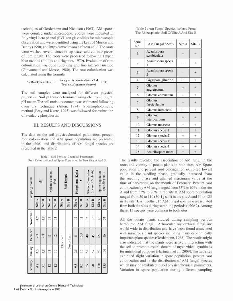
techniques of Gerdemann and Nicolson (1963). AM spores were counted under microscope. Spores were mounted in Poly vinyl lacto phenol (PVL) on glass slides for microscopic observation and were identified using the keys of Morton and Benny (1990) and http://www.invam.caf.wvu.edu/. The roots were washed several times in tap water and cut into pieces of 1cm length. The roots were processed following Trypan blue method (Philips and Hayman, 1970). Evaluation of root colonization was done following grid line intersect method (Giovannetti and Mosse, 1980). The root colonization was calculated using the formula
The soil samples were analyzed for different physical properties. Soil pH was determined using electronic digital pH meter. The soil moisture content was estimated following oven dry technique (Allen, 1974). Spectrophotometric method (Bray and Kurtz, 1945) was followed for estimation of available phosphorus.
III. RESULTS AND DISCUSSIONS
The data on the soil physicochemical parameters, percent root colonization and AM spore population are presented in the table1 and distributions of AM fungal species are presented in the table 2.
Table 1. Soil Physico-Chemical Parameters,Root Colonization And Spore Population In Two Sites A And B.
Sam
plin
g m
onth
s
pH
Moi
stur
e co
nten
t (%
)
Soil
Text
ure
Phos
phor
us (K
gha-
1)
%R
oot c
olon
izat
ion
(mea
n of
5 p
lant
s)
Spor
e po
pula
tion
(per
50
g so
il)
Site
A
Site
B
Site
A
Site
B
Site
A
Site
B
Site
A
Site
B
Site
A
Site
B
Site
A
Site
B
Nov
embe
r
4.7
4.8 14 13
Cla
y lo
am
Sand
y lo
am
12 11 33 35 48 55
Dec
embe
r
4.7
4.7 13 12 11 10.5 40 45 65 80
Janu
ary
4.5
4.8 11 10 9.5 10 52 57 90 100
Febr
uary
4.8
5.0 12 12 9.5
9.0 65 70 110
135
No.segments colonized with VAM% Root Colonization = × 100Total no.of segments observed
Table 2 : Am Fungal Species Isolated FromThe Rhizospheric Soil Of Site A And Site B
Serial No. AM Fungal Specis Site A Site B
1 Acaulospora scrobiculata + +
2 Acaulospora specis 1 + +
3 Acaulospora specis 2 - +
4 Gigaspora gilmorie + +
5 Glomus aggretgatum + +
6 Glomus coronatum - +
7 Glomus fasciculatum + +
8 Glomus intradices + +
9 Glomus microcarpum + +
10 Glomus mosseae + +11 Glomus specis 1 + +12 Glomus specis 2 + +13 Glomus specis 3 + +14 Glomus specis 4 + +15 Scutellospora rubra + +
The results revealed the association of AM fungi in the roots and vicinity of potato plants in both sites. AM Spore population and percent root colonization exhibited lowest value in the seedling phase, gradually increased from the seedling phase and attained maximum value at the time of harvesting on the month of February. Percent root colonization by AM fungi ranged from 33% to 65% in the site A and from 35% to 70% in the site B. AM spore population ranged from 50 to 110 (50-1g soil) in the site A and 54 to 125 in the site B. Altogether, 15 AM fungal species were isolated from both the sites during sampling periods (table 2). Among these, 13 species were common to both sites.
All the potato plants studied during sampling periods harboured AM fungi. Arbuscular mycorrhizal fungi are world wide in distribution and have been found associated with numerous plant species including many economically important plant species (Gerdemann, 1968). The results might also indicated that the plants were actively interacting with the soil to promote establishment of mycorrhizal symbiosis for nutritional purposes (Hartmann et al., 2009).The two sites exhibited slight variation in spore population, percent root colonization and in the distribution of AM fungal species which may be attributed to soil physicochemical parameters. Variation in spore population during different sampling
P 42International Journal on Current Science & Technology Vol - I l No- I l January-June’2013
months may also be due to the fact that different AM fungal species sporulate during different times of the year (Mangan et al., 2004). The highest degree of colonization of annual crops during the harvesting period may have a possible explanation of increasing the requirements of nutrients and water at this stage (She et al., 2007).
Glomus was found dominant genus in the present study comprising 67% of the total number of species. The dominance of the genus Glomus over other genus may be attributed to the fact that these are most wide spread fungi. Daniell et al.( 2001) suggested that Glomus may have the ability to recolonize roots from the mycelial fragments rapidly. Under Indian situation it has been observed that species representing the genus Glomus was dominant (Monoharachary et al., 2010). The dominance of Glomus over other genera in three rice fields of Barak valley has also been reported (Bhattacharjee and Sharma, 2011).
REFERENCES
[1] Allen, S.E., 1974. Chemical analysis of ecological materials. Blackwell scientific Publications, New Delhi.
[2] Bhattacharjee, S., and Sharma, G. D., 2011. The Vesicular Arbuscular Mycorrhiza associated with three cultivars of Rice (Oryza sativa L.). Indian J Microbiol. 51(3): 377-383.
[3] Daniell, T.J., Husband, R., Fitter, A.H., and Young, J.P.W., 2001. Molecular diversity of arbuscular mycorrhizal fungi colonizing arable crops. FEMS Microbiol Ecol. 36:203-209.
[4] Hartmann, A., Schmid, M., van Tuinea, D., Berg, G.,2009. Plant-driven selection of microbes. Plant Soil. 321: 235-257.
[5] Javot, H., Pumplin, N., an Gerdemann, J.W., and Nicolson, T. H., 1963. Spores of mycorrhizal Endogone extracted from soil by wet sieving and decanting. Transactions of the British Mycological Society. 46:235-244.
[6] Monoharachary, C., Kunwar, I.K., Tilak, K.V.B.R., and Adholeya. A., 2010. Arbuscular mycorrhizal fungi- taxonomy, diversity, conservation and multiplication. National Academy of Sciences, India. Sec.-B, 80: 1-13.
[7] Morton, J.B. and Benny, G.L., 1990. Revised classification of arbuscular mycorrhizal fungi (Zygomycetes): A new order, Glomales, two new suborder Glomineae and Gigasporinae and two new families Acaulosporaceae and Gigasporaceae with an emendation of Glomaceae. Mycotaxon 37: 471-491.
[8] Quilambo,O.A., 2000. Functioning of peanut (Arachis hypogeal.) under nutrient deficiency and drought stress in relation to symbiotic associations. Ph.D.thesis. University of Groningen. ISBN 903671284X.
[9] Gerdemann, J.W., and Nicolson, T. H., 1963. Spores of mycorrhizal Endogone extracted from soil by wet sieving and decanting. Transactions of the British Mycological Society. 46:235-244.
[10] Gerdemann, J.W., 1968. Vesicular arbuscular mycorrhiza and plant growth. Ann. Rev. Phytopathol. 6: 397-418.
[11] Giovannetti, M., and Mosse, B., 1980. An evaluation of techniques for measuring vesicular arbuscular mycorrhizal infection in roots. New Phytol. 84: 489-500.
[12] Mangan, S. A.,Eom, A-H., Adler, G. H., Yavitt, J. Herre, E. A., 2004. Diversity of arbuscular mycorrhizal fungi across a fragmented forest in Panama: insular spore communities differ from mainland communities. Oecologia. 141: 687-700.
[13] Phillips, J.M., and Hayman, D.J., 1970. Improved procedures for clearing and staining parasitic and vesicular-arbuscular mycorrhizal fungi for rapid assessment of infection. Transactions of the British Mycological Society. 55: 158- 161.
[14] Shi, Z.Y., Zhang, L.Y., Li, X.L.,Feng, G., Tian, C.Y., and Christie, P. 2007. Diversity of arbuscular mycorrhizal fungi associated with desert ephemerals in plant communities of Junggar Basin, north west China. Applied soil ecology. 35: 10-20.
P 43International Journal on Current Science & Technology
Vol - I l No- I l January-June’2013

P 44International Journal on Current Science & Technology Vol - I l No- I l January-June’2013

BIODIVERSITY AND CONSERVATIONSTRATEGIES OF HOME GARDEN CROPS IN MANIPUR
A Premila1 and GKN Chhetry2
Department of Botany, Standard College, Imphal1,Department of Life Sciences, Manipur University, Canchipur, Imphal2
Corresponding author E-mail: [email protected]
ABSTRACT
Home gardens in Manipur are organically managed gardens for the cultivation of variety of seasonal vegetables and other kitchen linked crops throughout the year by every household in the hills and plains for sequential production of vegetable crops. These traditionally managed varieties of vegetable crops are organic manure based prepared using produced using indigenous methods. Diversity of vegetable crops in home gardens include range of annual and perennial vegetables, oil yielding plants, common cereals in low scale and some traditional millets, fruits, medicinal plants, aromatic plants and other pest pathogen repellent plants, spicy crops etc. for ready consumption in the household. These crops are sequentially grown coinciding to the respective season for each crop and manage through traditional techniques using mulching, compost manuring of domesticated animals and other which are ecofriendly. Diversity of crops and their management strategies including management of pest pathogen in the homestead garden as well as in the storage are inventoried in length and discussed in detail with special emphasis on Indigenous Knowledge and Traditional Ecological Knowledge of organic home gardeners of Manipur.
Keywords: Home garden crops, Indigenous Knowledge, Traditional Ecological Knowledge, Biodiversity Conservation, etc.
I. NTRODUCTION
India, being an agricultural country where majority of the rural people reserve certain percentage of their agricultural land for the cultivation of variety of crops related to kitchen use around their homes as home garden crops for perennial source of vegetables. North east India inhabited by various ethnic communities maintain unique vegetable gardens for a perennial source of vegetables, pulses, spices, oil yielding plants including location specific fruits such as pineapple, pomegranate, papaya etc. besides maintaining far flung jhum land crops in hills and fertile paddy field in valley.
Biodiversity being a hot topic, well researched, discussed and documented by many in the state, region, country and the world as a whole (Fernandes and Nair, 1986; Myers et.al., 2000; Das and Das, 2005) but not much about the biodiversity of home garden crops. Further, diversity of edible and pest pathogen repellent crops maintained and preserved by every household of rural masses reflecting their indigenous culture and tradition represent significant component of agricultural biodiversity of crops grown without interference from modern chemicals including fertilizers, pesticides etc. in the form of home garden crops. As such, humble attempt is being made to document the diversity of home garden crops and its conservation strategies followed by the indigenous farmers in Manipur hills and valley in particular.
II. MATERIALS AND METHODS
Multistage random sampling technique was followed considering a block in a district and a village in a block is selected and a sample of five villages from each block was randomly selected in four valley districts namely Imphal East, Imphal West, Thoubal and Bishnupur of Manipur. Monthly survey was conducted to synchronize the availability of crops to these selected villages and interacted with the home gardeners as to the cultivation practices, organic maintenance of home garden crops, inputs of homemade organic fertilizers, sequence of crops grown followed by outputs of crops for use from their gardens. Inventory of diversity of crops including border crops of randomly selected home gardens of random villages was listed in detail in order to reflect the diversity of home garden crops and their conservation strategies of indigenous people.
III. RESULT
As many as 28 vegetable crops meant for the consumption of green vegetables were found in a typical home garden maintained by home gardeners in Manipur valley (Table 1). Vegetables belonging to Cucurbitaceae and Brassicaceae
P 45International Journal on Current Science & Technology
Vol - I l No- I l January-June’2013
were more followed by Solanaceae and Malvaceae and many other families numbering as many as eight were found in different seasons- Spring (March to May), Summer (June to August), Autumn (September to November) and Winter (December to February). Spring and summer seasons contributed highest number (48 each) of plant species whereas winter season listed lowest number (46 each) of plant species.
Crop under pulses is also important home garden crops in Manipur valley which are as many as ten under the family Fabaceae. Of these, Phaseolus vulgaris, commonly called French bean is grown throughout the year. A typical home garden also found to have a number of oil yielding crops which are as many as six belonging to five families. Spicy crop is another important home garden crop of which Allium ascalonium is an indigenous variety cultivated by home gardeners for multiple uses throughout the year. As many as sixteen spicy crops are found in a typical Meetei home garden in the rural areas of Manipur valleys.
As the home garden crops are organically managed, certain medicinal/ pest pathogen and insect repellent plant as many as thirteen were found in the biodiversity of home garden crops. Vitamin yielding plants such as fruits numbering eighteen were found in a typical home garden which is usually grown in the periphery of the garden. Plants of aesthetic value which includes flowers of different varieties are also found in backyard and surroundings of home garden. Interestingly, indigenous home gardeners grow some crops as border crops that include typical bamboo species, banana plants, etc. The percentage contribution of these home garden crops represented in a pi diagram (Fig. 1) showed maximum contribution by vegetables (25.22%) followed by fruits (16.21%), spicy crops (13.51%), medicinal plants (11.71%), flowers (11.71%), pulses (9.01%), border plants (7.21%) and least by oil yielding plants (5.4%) etc.
Indigenous farmers for that matter home gardener conserved and preserved gene banks of home garden crops since generations and managed the same in their indigenous way in pure form. As these traditionally preserved home garden seed banks are well adapted to natural way of farming i.e. organic farming, indigenous home gardeners followed specific conservation strategies of these crops by way of organic methods only. As such, they are afraid of using modern chemicals either as fertilizers for plant nutrients or pesticides/ fungicides for protection of crops against pest pathogens. Instead they conserved and managed their home gardens through the use of homemade organic manures and by growing pest pathogen repellent crops in the periphery of the home gardens which not only repels the attack of pest pathogens but also protects the crops from other domestic animals. This unique strategy followed by organic home
gardeners are ecofriendly and sustainable for use at the household level.
IV. DISCUSSION
Research on biodiversity related to home garden crops is very much limited to few workers in the field. Only astray information about the biodiversity of home garden crops is available from this region. Das and Das, 2005 opined that home garden are conservation site of large number of crops and reported as many as 122 crops from a typical home garden in a Barak valley of Assam whereas Chhetry and Belbahri, 2009 reported certain pest pathogen repellent home garden crops managed by the people of North East India. These two papers provided the benchmark information related to the biodiversity and conservation strategies of home garden crops in North East India. Interestingly, home garden crops are managed organically using available plant resources as mulching material, preparation of organic manures, preparation of biopesticides, etc. which are ecofriendly and ecologically sustainable practices. They make use of available plant resources which act as pest pathogen repellent for the temporary storage of home garden crops free from insect pest and pathogen by growing a number of pest pathogen and insect repellent medicinal plants. This indigenous technique for the production of home garden crop is mandatory for the home gardeners as they not only afford costly modern chemicals but also afraid of losing the traditional genetic materials due to application of chemicals. Moreover, they are scared of health related diseases due to the consumption of chemical used home garden crops because they cannot afford the costly medicines if at all they suffer from health related diseases due to chemical residues. Consciousness about the importance of home garden crops being realized by international communities primarily for the reason that home garden crops are purely organic, healthy and fresh vegetables for day to day consumption have been emphasized in the paper by Fernandes and Nair, 1986 which corroborates the findings in this paper.
V. ACKNOWLEDGEMENT
The first author is thankful to UGC, New Delhi for financial assistance and to Principal, Standard College, Imphal for laboratory facilities.
Table 1: Diversity of crops in a typical home garden in Manipur Valley.
Scientific/Botanical name Family name Local name
Vegetables
1 Amaranthus spinosus Amaranthaceae Chengkruk
2 Amorphophallus companulatus
Araceae Haopaan
3 Benincasa hispida Cucurbitaceae Torbot
P 46International Journal on Current Science & Technology Vol - I l No- I l January-June’2013
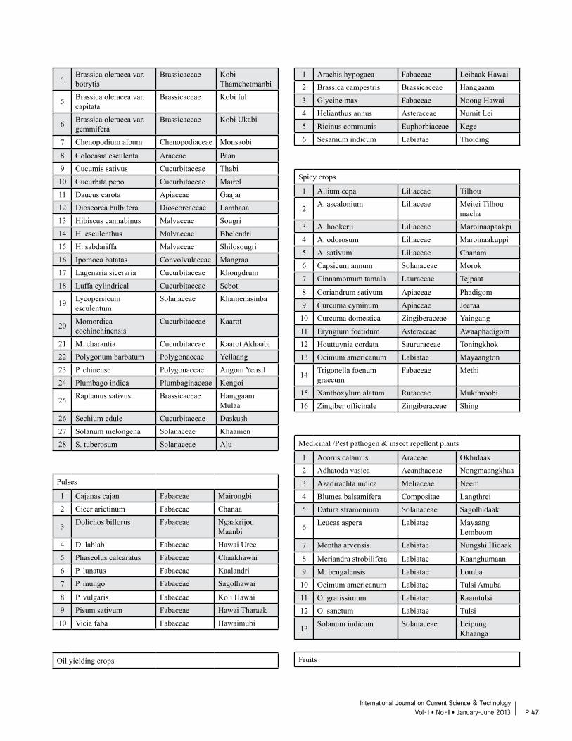
4 Brassica oleracea var. botrytis
Brassicaceae Kobi Thamchetmanbi
5 Brassica oleracea var. capitata
Brassicaceae Kobi ful
6 Brassica oleracea var. gemmifera
Brassicaceae Kobi Ukabi
7 Chenopodium album Chenopodiaceae Monsaobi
8 Colocasia esculenta Araceae Paan9 Cucumis sativus Cucurbitaceae Thabi10 Cucurbita pepo Cucurbitaceae Mairel11 Daucus carota Apiaceae Gaajar12 Dioscorea bulbifera Dioscoreaceae Lamhaaa13 Hibiscus cannabinus Malvaceae Sougri14 H. esculenthus Malvaceae Bhelendri15 H. sabdariffa Malvaceae Shilosougri16 Ipomoea batatas Convolvulaceae Mangraa17 Lagenaria siceraria Cucurbitaceae Khongdrum18 Luffa cylindrical Cucurbitaceae Sebot
19 Lycopersicum esculentum
Solanaceae Khamenasinba
20 Momordica cochinchinensis
Cucurbitaceae Kaarot
21 M. charantia Cucurbitaceae Kaarot Akhaabi22 Polygonum barbatum Polygonaceae Yellaang23 P. chinense Polygonaceae Angom Yensil24 Plumbago indica Plumbaginaceae Kengoi
25 Raphanus sativus Brassicaceae Hanggaam Mulaa
26 Sechium edule Cucurbitaceae Daskush27 Solanum melongena Solanaceae Khaamen28 S. tuberosum Solanaceae Alu
Pulses
1 Cajanas cajan Fabaceae Mairongbi2 Cicer arietinum Fabaceae Chanaa
3 Dolichos biflorus Fabaceae Ngaakrijou Maanbi
4 D. lablab Fabaceae Hawai Uree5 Phaseolus calcaratus Fabaceae Chaakhawai6 P. lunatus Fabaceae Kaalandri
7 P. mungo Fabaceae Sagolhawai
8 P. vulgaris Fabaceae Koli Hawai 9 Pisum sativum Fabaceae Hawai Tharaak10 Vicia faba Fabaceae Hawaimubi
Oil yielding crops
1 Arachis hypogaea Fabaceae Leibaak Hawai2 Brassica campestris Brassicaceae Hanggaam3 Glycine max Fabaceae Noong Hawai4 Helianthus annus Asteraceae Numit Lei5 Ricinus communis Euphorbiaceae Kege6 Sesamum indicum Labiatae Thoiding
Spicy crops
1 Allium cepa Liliaceae Tilhou
2 A. ascalonium Liliaceae Meitei Tilhou macha
3 A. hookerii Liliaceae Maroinaapaakpi4 A. odorosum Liliaceae Maroinaakuppi5 A. sativum Liliaceae Chanam6 Capsicum annum Solanaceae Morok
7 Cinnamomum tamala Lauraceae Tejpaat
8 Coriandrum sativum Apiaceae Phadigom9 Curcuma cyminum Apiaceae Jeeraa10 Curcuma domestica Zingiberaceae Yaingang11 Eryngium foetidum Asteraceae Awaaphadigom12 Houttuynia cordata Saururaceae Toningkhok13 Ocimum americanum Labiatae Mayaangton
14 Trigonella foenum graecum
Fabaceae Methi
15 Xanthoxylum alatum Rutaceae Mukthroobi16 Zingiber officinale Zingiberaceae Shing
Medicinal /Pest pathogen & insect repellent plants
1 Acorus calamus Araceae Okhidaak2 Adhatoda vasica Acanthaceae Nongmaangkhaa3 Azadirachta indica Meliaceae Neem4 Blumea balsamifera Compositae Langthrei5 Datura stramonium Solanaceae Sagolhidaak
6 Leucas aspera Labiatae Mayaang Lemboom
7 Mentha arvensis Labiatae Nungshi Hidaak
8 Meriandra strobilifera Labiatae Kaanghumaan9 M. bengalensis Labiatae Lomba10 Ocimum americanum Labiatae Tulsi Amuba11 O. gratissimum Labiatae Raamtulsi12 O. sanctum Labiatae Tulsi
13 Solanum indicum Solanaceae Leipung Khaanga
Fruits
P 47International Journal on Current Science & Technology
Vol - I l No- I l January-June’2013
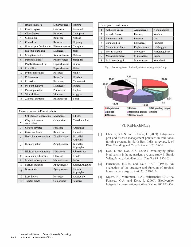
Home garden border crops
1 Adhatoda vasica Acanthaceae Nongmangkha2 Arundo donax Poaceae Yenthou3 Bamboosa tulda Poaceae Waa4 Canna indica Cannaceae Laphurit5 Manihot esculenta Euphorbiaceae U-Manggra6 Morus australis Moraceae Kaabrangchaak
7 Musa paradisiacal Mimosaceae Laphu
8 Parkia roxburghii Mimosaceae Yongchaak
Fig. 1: Percentage contribution by different categories of crops
VI. REFERENCES
[1] Chhetry, G.K.N. and Belbahri, L. (2009). Indigenous pest and disease management practices in traditional farming systems in North East India- a review. J. of Plant Breeding and Crop Science. 1(3): 28-38.
[2] Das, T. and Das, A.K. (2005) Inventorying plant biodiversity in home gardens : A case study in Barak Valley, Assam, North-East India. Curr. Sci. 98 : 155-163.
[3] Fernandes, E.C.M. and Nair, P.K.R. (1986). An evaluation of the structure and function of tropical home gardens. Agric. Syst. 21 : 279-310.
[4] Myers, N., Mittermeir, R.A., Mittermeier, C.G., da Fonseca, G.A. and Kent, J. (2000). Biodiversity hotspots for conservation priorities. Nature. 403:853-856.
1 Brucia javanica Simaroubaceae Heining2 Carica papaya Caricaceae Awaathabi3 Citrus lemon Rutaceae Champraa4 C. maxima Rutaceae Nobaab5 C. medica Rutaceae Heijaang6 Elaeocarpus floribundus Elaeocarpaceaz Chorphon
7 Eugenia janbolana Myrtaceae Jaam
8 Mangifera indica Anacardiaceae Heinou9 Passiflora edulis Passifloraceae Sitaaphal10 Phyllanthus acidu s Euphorbiaceae Gihori11 P. emblica Euphorbiaceae Heikru12 Prunus armeniaca Rosaceae Malhei13 P. domestica Rosaceae Heikhaa14 P. persica Rosaceae Choombrei15 Psidium guajava Myrtaceae Pungtol16 Punica granatum Punicaceae Kaphoi17 Vitis vinifera Vitaceae Anggoor18 Ziziphus auritiana Rhamnaceae Boroi
Flowers/ ornamental/ scenic plants
1 Callistemon lanceolatus Myrtaceae Liklilei
2 Chrysanthemum coronarium
Compositae Chandramukhi
3 Clitoria ternatea Fabaceae Aparajitaa4 Gardenia florida Rubiaceae Kaboklei
5 Hedychium coronarium Zingiberaceae Takhellei Angouba
6 H. marginatum Zingiberaceae Takhellei Angangba
7 Hibiscus rosa chinensis Malvaceae Jubaakusum
8 Jasminum pubescens Oleaceae Kundo9 Michelia champaca Magnoliaceae Leihao10 Nerium indicum Apocynaceae Kabirei Angouba
11 N. oleander Apocynaceae Kabirei Angangba
12 Rosa indica Rosaceae Aatorgulab13 Tagetes erecta Compositae Sanaarei
P 48International Journal on Current Science & Technology Vol - I l No- I l January-June’2013
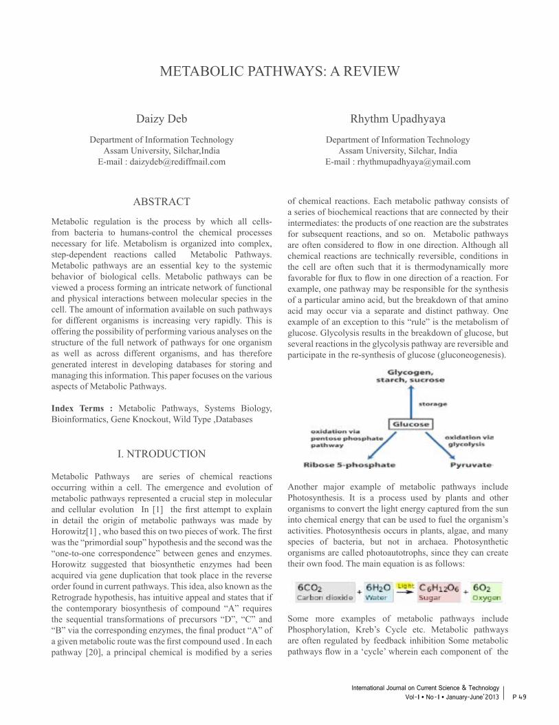
METABOLIC PATHWAYS: A REVIEW
Daizy Deb
Department of Information TechnologyAssam University, Silchar,India
E-mail : [email protected]
Rhythm Upadhyaya
Department of Information TechnologyAssam University, Silchar, India
E-mail : [email protected]
ABSTRACT
Metabolic regulation is the process by which all cells-from bacteria to humans-control the chemical processes necessary for life. Metabolism is organized into complex, step-dependent reactions called Metabolic Pathways. Metabolic pathways are an essential key to the systemic behavior of biological cells. Metabolic pathways can be viewed a process forming an intricate network of functional and physical interactions between molecular species in the cell. The amount of information available on such pathways for different organisms is increasing very rapidly. This is offering the possibility of performing various analyses on the structure of the full network of pathways for one organism as well as across different organisms, and has therefore generated interest in developing databases for storing and managing this information. This paper focuses on the various aspects of Metabolic Pathways.
Index Terms : Metabolic Pathways, Systems Biology, Bioinformatics, Gene Knockout, Wild Type ,Databases
I. NTRODUCTION
Metabolic Pathways are series of chemical reactions occurring within a cell. The emergence and evolution of metabolic pathways represented a crucial step in molecular and cellular evolution In [1] the first attempt to explain in detail the origin of metabolic pathways was made by Horowitz[1] , who based this on two pieces of work. The first was the “primordial soup” hypothesis and the second was the “one-to-one correspondence” between genes and enzymes. Horowitz suggested that biosynthetic enzymes had been acquired via gene duplication that took place in the reverse order found in current pathways. This idea, also known as the Retrograde hypothesis, has intuitive appeal and states that if the contemporary biosynthesis of compound “A” requires the sequential transformations of precursors “D”, “C” and “B” via the corresponding enzymes, the final product “A” of a given metabolic route was the first compound used . In each pathway [20], a principal chemical is modified by a series
of chemical reactions. Each metabolic pathway consists of a series of biochemical reactions that are connected by their intermediates: the products of one reaction are the substrates for subsequent reactions, and so on. Metabolic pathways are often considered to flow in one direction. Although all chemical reactions are technically reversible, conditions in the cell are often such that it is thermodynamically more favorable for flux to flow in one direction of a reaction. For example, one pathway may be responsible for the synthesis of a particular amino acid, but the breakdown of that amino acid may occur via a separate and distinct pathway. One example of an exception to this “rule” is the metabolism of glucose. Glycolysis results in the breakdown of glucose, but several reactions in the glycolysis pathway are reversible and participate in the re-synthesis of glucose (gluconeogenesis).
Another major example of metabolic pathways include Photosynthesis. It is a process used by plants and other organisms to convert the light energy captured from the sun into chemical energy that can be used to fuel the organism’s activities. Photosynthesis occurs in plants, algae, and many species of bacteria, but not in archaea. Photosynthetic organisms are called photoautotrophs, since they can create their own food. The main equation is as follows:
Some more examples of metabolic pathways include Phosphorylation, Kreb’s Cycle etc. Metabolic pathways are often regulated by feedback inhibition Some metabolic pathways flow in a ‘cycle’ wherein each component of the
P 49International Journal on Current Science & Technology
Vol - I l No- I l January-June’2013
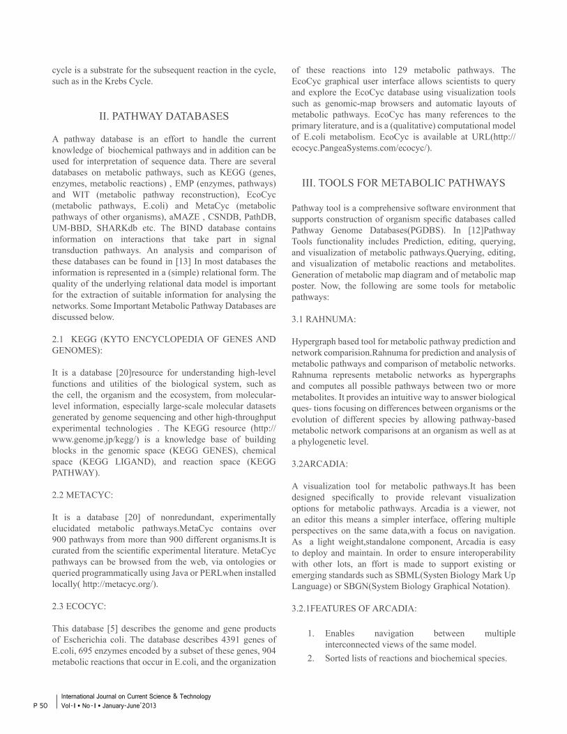
cycle is a substrate for the subsequent reaction in the cycle, such as in the Krebs Cycle.
II. PATHWAY DATABASES
A pathway database is an effort to handle the current knowledge of biochemical pathways and in addition can be used for interpretation of sequence data. There are several databases on metabolic pathways, such as KEGG (genes, enzymes, metabolic reactions) , EMP (enzymes, pathways) and WIT (metabolic pathway reconstruction), EcoCyc (metabolic pathways, E.coli) and MetaCyc (metabolic pathways of other organisms), aMAZE , CSNDB, PathDB, UM-BBD, SHARKdb etc. The BIND database contains information on interactions that take part in signal transduction pathways. An analysis and comparison of these databases can be found in [13] In most databases the information is represented in a (simple) relational form. The quality of the underlying relational data model is important for the extraction of suitable information for analysing the networks. Some Important Metabolic Pathway Databases are discussed below. 2.1 KEGG (KYTO ENCYCLOPEDIA OF GENES AND GENOMES):
It is a database [20]resource for understanding high-level functions and utilities of the biological system, such as the cell, the organism and the ecosystem, from molecular-level information, especially large-scale molecular datasets generated by genome sequencing and other high-throughput experimental technologies . The KEGG resource (http://www.genome.jp/kegg/) is a knowledge base of building blocks in the genomic space (KEGG GENES), chemical space (KEGG LIGAND), and reaction space (KEGG PATHWAY). 2.2 METACYC:
It is a database [20] of nonredundant, experimentally elucidated metabolic pathways.MetaCyc contains over 900 pathways from more than 900 different organisms.It is curated from the scientific experimental literature. MetaCyc pathways can be browsed from the web, via ontologies or queried programmatically using Java or PERLwhen installed locally( http://metacyc.org/). 2.3 ECOCYC:
This database [5] describes the genome and gene products of Escherichia coli. The database describes 4391 genes of E.coli, 695 enzymes encoded by a subset of these genes, 904 metabolic reactions that occur in E.coli, and the organization
of these reactions into 129 metabolic pathways. The EcoCyc graphical user interface allows scientists to query and explore the EcoCyc database using visualization tools such as genomic-map browsers and automatic layouts of metabolic pathways. EcoCyc has many references to the primary literature, and is a (qualitative) computational model of E.coli metabolism. EcoCyc is available at URL(http://ecocyc.PangeaSystems.com/ecocyc/).
III. TOOLS FOR METABOLIC PATHWAYS
Pathway tool is a comprehensive software environment that supports construction of organism specific databases called Pathway Genome Databases(PGDBS). In [12]Pathway Tools functionality includes Prediction, editing, querying, and visualization of metabolic pathways.Querying, editing, and visualization of metabolic reactions and metabolites. Generation of metabolic map diagram and of metabolic map poster. Now, the following are some tools for metabolic pathways:
3.1 RAHNUMA:
Hypergraph based tool for metabolic pathway prediction and network comparision.Rahnuma for prediction and analysis of metabolic pathways and comparison of metabolic networks. Rahnuma represents metabolic networks as hypergraphs and computes all possible pathways between two or more metabolites. It provides an intuitive way to answer biological ques- tions focusing on differences between organisms or the evolution of different species by allowing pathway-based metabolic network comparisons at an organism as well as at a phylogenetic level.
3.2ARCADIA:
A visualization tool for metabolic pathways.It has been designed specifically to provide relevant visualization options for metabolic pathways. Arcadia is a viewer, not an editor this means a simpler interface, offering multiple perspectives on the same data,with a focus on navigation.As a light weight,standalone component, Arcadia is easy to deploy and maintain. In order to ensure interoperability with other lots, an ffort is made to support existing or emerging standards such as SBML(Systen Biology Mark Up Language) or SBGN(System Biology Graphical Notation). 3.2.1FEATURES OF ARCADIA:
1. Enables navigation between multiple interconnected views of the same model.2. Sorted lists of reactions and biochemical species.
P 50International Journal on Current Science & Technology Vol - I l No- I l January-June’2013
3. Detailed properties of selected elements.4. Graphic representations of the whole network.5. Local Maps for groups of neighbouring molecules.
3.3 UTOPIA:
An open source, interoperable set of desktop tools for protein analysis, built according to the model/view/controller pattern. 3.4 PW COMP:
In [7] A graph comparative metabolic pathway tool.Along with the recent explosion of available genetic sequence information for a variety of organisms, there has been a similar increase in the information available related to the functional roles of proteins in metabolism. Many databases exist that provide rich sources of information for the constituent genes and reactions in the metabolisms of many organisms. This information has the potential to lead to more insight into the functional mechanisms of cellular metabolism. By developing a flexible method for comparing metabolic processes among different organisms, new insight into their functional mechanisms and evolutionary relationships may be uncovered. PWComp provides an interface for users to investigate the similarity between metabolic pathways contained in the BioCyc database. It implements the graph comparative algorithm described by “Heymans” that computes a similarity score using the similarity between nodes of the ‘metabolic graph’ and the structure of the nodes’ connections. PWComp consists of three major components, each written in java: (i) A set of data structures that contain information about the pathways and their constituent components (ii) a computational engine that executes the Heymans Algorithm, and (iii) a GUI that allows the user to navigate the database of information and the similarity measurements between pathways.
3.5 ELEMENTARY MODE ANALYSIS:
In [18] A useful metabolic pathway analysis tool for characterizing cellular metabolism.Useful metabolic pathway analysis tool to identify the structure of a metabolic network that links the cellular phenotype to the corresponding genotype. 3.6 KATSURA:
In [13] KEGG pathway analysis and expression analysis It overlays microarray gene expression data, proteomics and similar biological data onto metabolic pathways.
3.7 PATHWAY HUNTER TOOL:
In [15] Pathway hunter tool is a fast ,robust and user friendly tool to analyse the shortest path analysis for one or more organisms or can build virtual organisms(networks) using eenzymes,using pathway hunter tool,the user can calculate the average shortest path, average alternate paths and the top hubs in the metabolic networks.
IV. SOME YEAR-WISE WORKS 1991: In [2] Yogurt and similar fermented milk products have been very popular for a long time. “yogurt” can be used legally only to designate the product resulting from milk fermentation brought about exclusively with 2 thermophilic lactic acid bacteria, Streptococcus and Lactobacillus, which must be found alive in the final product of yogurt . We review here recent data on some of the metabolic and biochemical aspects’ of these starter bacteria in relation to yogurt manufacture. Metabolic pathways of lactose, glucose and galactose utilization. interaction between yogurt bacteria is a good example of integrated metabolism in a mixed culture of lactic acid bacteria, but our knowledge of stimulation is still incomplete. Studies have led to a better understanding of sorne metabolic and biochemical aspects of these bacteria that control their growth, especially in mixed cultures. For instance, lactose and galactose metabolism have been weil studied at both the biochemical and molecular levels. the characterization of inhibitory substances which may be produced would be very useful (a)for a better understanding of the relationship between the yogurt bacteria, and (b)for their action on other micro-organisms associated with yogurt bacteria for the manufacture of several fermented milk products.Finally, progress in genetic studies should contribute to better knowledge on the yogurt bacteria and their growth and activity in milk.
1999: In [15] There have been recent advances in metabolic flux analysis. In particular, the marriage of traditional flux balancing with NMR isotopomer distribution analysis holds great promise for the detailed quantification of physiology. Nevertheless, flux analysis yields only static snap-shots of metabolism. To robustly predict the time evolution of metabolic networks, dynamic mathematical models, especially those that contain a description of both gene expression as well as enzyme activity, must be utilized. When mechanistic control and regulatory information is not available, heuristic-based methods, such as the cybernetic framework, can be employed to describe the action of these control mechanisms. In the ‘high-information’ future, as more biological information becomes available, such heuristic-based approaches can be replaced by mechanistic mass-action representations of physiology that stem directly from genetic sequence.
P 51International Journal on Current Science & Technology
Vol - I l No- I l January-June’2013
2000: In [16] We have studied the metabolic behavior and capabilities of E. coli MG1655 in silico and formulated experiments that directly test the optimal growth of E. coli. For the considered growth conditions, quantitative predictions of the substrate and oxygen uptake rates, byproduct secretion rates, and cellular growth rates were obtained. Two metabolic fluxes corresponding to the substrate uptake rate (acetate/succinate and oxygen uptake) and the growth flux were chosen to define the three-dimensional phenotype phase surface. Under the examined growth conditions, the hypothesis that E. coli optimizes its growth rate subject to systemic capacity and stoichiometric constraints was consistent with the experimental data. Thus, for the growth conditions considered, it was possible to use an in silico metabolic reconstruction to quantitatively interpret metabolic physiology.The in silico approach utilized is a departure from traditional approaches to the detailed modeling of physicochemical systems.
2001: In [9] The large volume of genome-scale data that is being produced and made available in databases on the World Wide Web is demanding the development of integrated mathematical models of cellular processes. The analysis of reconstructed metabolic networks as systems leads to the development of an in silico or computer representation of collections of cellular metabolic constituents, their interactions and their integrated function as a whole. The use of quantitative analysis methods to generate testable hypotheses and drive experimentation at a whole-genome level signals the advent of a systemic modeling approach to cellular and molecular biology.
2004 : In [4] the post-genomic era, several profiling tools have been developed to provide a more comprehensive picture of tumour development and progression. The global analysis of metabolites, such as by mass spectrometry and high-resolution 1H nuclear magnetic resonance spectroscopy, can be used to define the metabolic phenotype of cells, tissues or organisms. These ‘metabolomic’ approaches are providing important information about tumorigenesis, revealing new therapeutic targets and will be an important component of automated diagnosis.
2002 : In [19] MOMA is an additional option, based on a simple hypothesis about the response to metabolic alterations. This approach seems especially relevant for analyzing gene deletions, but its possible future extensions could help understand metabolic networks for a wider range of perturbations.
2005 : In[14] We introduced ROOM as a model for predicting the steady-state behavior of metabolic networks in response to gene knockouts and compared its accuracy with FBA and MOMA. We find that MOMA provides accurate
predictions for transient growth rates, observed during the early postperturbation state, whereas ROOM and FBA more successfully predict final steady-state growth rates. Consequently, both ROOM and FBA provide more accurate lethality predictions. ROOM is shown to provide more accurate flux predictions than FBA and MOMA for the final metabolic steady state.Additional work is required to find metrics that better approximate the complex adaptation of the metabolic network after the knockout and to understand their possible biological consequences.
2010 : In [17] Metabolic pathway analysis of the essential proteins in Staphylococcus aureus done by KEGG Automatic Annotation Server(KAAS). A result of comparative analysis of the metabolic pathways of the host and pathogen by using the Kyoto Encyclopedia of Genes and Genomes (KEGG) pathway database reveals some pathways that are unique to Staphylococcus aureus and are not present in the humans like D-Alanine metabolism, Peptidoglycan biosynthesis, Phosphotransferase system (PTS), Bacterial secretion system and Two-component system . This small group of proteins is required to be further verified for their role in Staphylococcus aureus survival and virulence by mutagenesis study. Further we analyze our essential enzymes of DEG database result against the drug bank database, and we identified about 8 approved drug target and 24 small molecule drug target.
2008 : In [15] The method based on decomposition of a stoichiometric matrix of metabolic pathways provides us a wide variety of information for comprehending the complex topology of metabolic pathways in a systematic way . The MAPLE program we have developed is easy to use and can be employed to derive all of the conservation relationships for a given metabolic pathway automatically. Furthermore it is able to compute conservation relationships of any metabolic pathways which may include unlimited steps and intermediate metabolites. There is certainly scope for the application of modern computer algebra techniques to analyze a complex metabolic system but at present it is a largely unexploited field MAPLE as a computer algebra system provides a powerful tool for analyzing such systems. We hope that this program may make a partial contribution in this field.
2012 : In [21] kinetic modelling of plant metabolic pathways as a tool for analysing their control and regulation. An overview of different modelling strategies is presented, starting with those approaches that only require a knowledge of the network stoichiometry; these are referred to as structural. Flux-balance analysis, metabolic flux analysis using isotope labelling, and elementary mode analysis are briefly mentioned as three representative examples. The main focus of this paper, however, is a discussion of kinetic modelling, which requires, in addition to the stoichiometry, a knowledge
P 52International Journal on Current Science & Technology Vol - I l No- I l January-June’2013
of the kinetic properties of the constituent pathway enzymes. The different types of kinetic modelling analysis, namely time-course simulation, steady-state analysis, and metabolic control analysis, are explained in some detail. An overview is presented of strategies for obtaining model parameters, as well as software tools available for simulation of such models. The kinetic modelling approach is exemplified with discussion of three models from the general plant physiology literature. With the aid of kinetic modelling it is possible to perform a control analysis of a plant metabolic system, to identify potential targets for biotechnological manipulation, as well as to ascertain the regulatory importance of different enzymes (including isoforms of the same enzyme) in a pathway. Finally, a framework is presented for extending metabolic models to the whole-plant scale by linking biochemical reactions with diffusion and advective flow through the phloem. Future challenges include explicit modelling of subcellular compartments, as well as the integration of kinetic models on the different levels of the cellular and organizational hierarchy.
V. CONCLUSION
The management of biochemical reactions with enzymes is an important part of cellular maintenance. Enzymatic activity allows a cell to respond to changing environmental demands and regulate its metabolic pathways, both of which are essential to cell survival. Sometimes, human metabolism is excessively slow or fast due to disease states and may be treated medically. Some drugs or nutritional substances can be said to boost metabolic rates by changing the rate of pathways involved with carbohydrate or fat digestion. In the course of molecular and cellular evolution different mechanisms and different forces might have concurred in the arisal of new metabolic abilities and shaping of metabolic routes. Analysing these networks remains far from straightforward owing to the nature of the databases, which are often heterogeneous, incomplete or inconsistent. Metabolic pathway analysis is hence a challenging problem in systems biology and in bioinformatics.
VI. REFERENCES
[1] Renato Fani, Marco Fondi ,Laboratory of Microbial and Molecular Evolution, Department of Evolutionary Biology, Via Romana , University of Florence, Italy, “Origin and evolution of metabolic pathways” Proceedings of the Physics of Life Reviews 6 (2009) 23-52.
[2] A Zourari *, JP Accolas, MJ Desmazeaud , Station de Recherches Laitières, INRA, 78352 Jouy-en-Josas Cedex, France “Metabolism and biochemical
characteristics of yogurt bacteria. A review” proceedings of the Lait (1992) 72,1-34 © Elsevier/ INRA,Review article
[3] Daniel I. BenjaminBenjamin F. Cravatt Daniel K. Nomura, “Global Profiling Strategies for Mapping Dysregulated Metabolic Pathways in Cancer”Proceedings of Cell Metabolism, Volume 16, Issue 5, 565-577, 11 October 2012, Copyright © 2012 Elsevier Inc. All rights reserved. 10.1016/j. cmet.2012.09.013
[4] Julian L. Griffin1 & John P. Shockcor2 Department of Biochemistry, University of Cambridge,TennisCourt Road, CB2 1GA, UK. Bruker Biospin, 15, Fortune Drive, Billerica, Massachusetts 01821, USA. “Metabolic profiles of cancer cells” proceedings of the Nature Reviews Cancer 4, 551-561 (July 2004) | doi:10.1038/nrc1390
[5] Peter D. Karp*, Monica Riley1, Suzanne M. Paley, Alida Pellegrini-Toole1,Markus Krummenacker “Eco Cyc: Encyclopedia of Escherichia coli genes and metabolism” proceedings of the Nucleic Acids Res. (1999) 27 (1):55-58.doi: 10.1093/nar/27.1.55
[6] Albert Sorribas†, Michael A. Savageau,Department of Microbiology and Immunology, The University of Michigan, Ann Arbor, Michigan 48109-0620, USA “Strategies for representing metabolic pathways within biochemical systems theory: Reversible pathways” proceedings of the 6th International Conference on Mathematical Modelling, St. Louis, Missouri, 4-7 August 1987, and the 1st IFAC Symposium on Modelling and Control in Biomedical Systems, Venice, Italy, 6-9 April 1988.
[7] JACQUES VAN HELDEN,LORENZ WERNISCH, DAVID GILBERT AND SHOSHANA WODAK European Bioinformatics Institute (EBI). Genome Campus-Hinxton Cambridge CB10 1SD - UK., Unité de Conformation des Macromolécules Biologiques. Université Libre de Bruxelles.50 av. F.D. Roosevelt. B-1050 Bruxelles. Belgium. School of Crystallography. Birkbeck College, University of London, Malet Street, London WC1E 7HX, UK., Department of Computing, City University, Northampton Square, London EC1V 0HB, UK. “Graph-based analysis of metabolic networks”
[8] F. J. Planes J.E. Beasley, Mathematical Sciences, Brunel University, Uxbridge, UB8 3PH, UK. “A critical examination of stoichiometric and path-finding approaches to metabolic pathways” proceedings of Briefing in Bioinformatics (2008) 9 (5): 422-436. doi: 10.1093/bib/bbn018 First published online: April 24, 2008
[9] Markus W. Coverta, Christophe H. Schillinga, Iman
P 53International Journal on Current Science & Technology
Vol - I l No- I l January-June’2013
Familia,Jeremy S. Edwardsb ,Igor I. Goryanin, Evgeni Selkovd ,Bernhard O. Palssona a Dept Bioengineering, University of California, San Diego, La Jolla, CA 92093-0412, USA,b Dept Chemical Engineering, University of Delaware, Newark, DE 19716, USA,c RIS Informatics, GlaxoWellcome, Stevenage, UK SG2 9AR d Integrated Genomics, 2201 W. Campbell Park Dr., Chicago, IL 60612, USA “Metabolic modeling of microbial strains in silico” proceedings of Trends in biochemical sciences volume 26,issue 3, march 2001.
[10] J Varnera,D Ramkrishnab ,Institute of Biotechnology, ETH-Zurich, Zurich, Switzerland CH-8093, School of Chemical Engineering, Purdue University, West Lafayette, IN 47907, USA “Mathematical models of metabolic pathways” proceedings of Current Opinion in Biotechnology Volume 10, Issue 2, 1 April 1999, Pages 146-150.
[11] Ulrike Wittig, European Media Laboratory, Villa Bosch, Schloss-Wolfsbrunnenweg 33, 69118 Heidelberg, Germany “Analysis and comparison of metabolic pathway databases” Proceedings of the Briefings in Bioinformatics (2001) 2 (2): 126-142. doi: 10.1093/bib/2.2.126
[12] Yves Deville,Computing Science and Engineering Department,Université catholique de Louvain Place Saint-Barbe 2, B-1348 Louvain-la-Neuve, Belgium, David Gilbert, Bioinformatics Research Centre, Department of Computing Science,University of Glasgow 17 Lilybank Gardens,Glasgow G12 8QQ, Scotland, UK, Jacques van Helden, Shoshana J. Wodak Service de Conformation de Macromolécules Biologiques et Bioinformatique CP263, Université Libre de Bruxelles Blvd du Triomphe,B-1050 Bruxelles, Belgium “An Overview of Data Models for the Analysis of Biochemical Pathways”
[13] Tomer Shlomi, Omer Berkman and Eytan Ruppin Raymond and Beverly Sackler Faculty of Exact Sciences Tel Aviv University, Tel Aviv 69978, Israel “Regulatory on/off minimization of metabolic flux change after genetic perturbations” proceedings of The National Academy of Sciences of the USA(2005)
[14] Mustafa BAYRAM* & Burcu ÖZYURT SERİM** Yildiz Technical University, Faculty of Arts and Sciences, Department of Mathematics, 34210 Davutpasa-Istanbul/ Turkey, **Halic University Faculty of Business Administration Beyoglu-İstanbul/ Turkey “MATHEMATICAL MODELING OF METABOLIC PATHWAYS”
[15] Jeremy S. Edwards1, 2, Rafael U. Ibarra1, and Bernhard O. Palsson1* 1Department of Bioengineering, University of California, San Diego, 9500 Gilman Drive, La Jolla, CA 92093-0412. 2Department of Chemical Engineering, University of Delaware, Newark, DE 19716. “In silico predictions of Escherichia coli metabolic capabilities are consistent with experimental data” proceedings of the 2001 Nature Publishing Group http://biotech.nature.com
[16] V. K. Morya*, Varun Dewaker, S. D. Mecarty and Raghuvir SinghDepartment of Molecular and Cellular Engineering Jacob School of Biotechnology and Bioengineering Sam Higginbotom Institute of Agriculture, Technology & Sciences,Allahabad, Uttar Pradesh, INDIA “In silico Analysis of Metabolic Pathways for Identification of Putative Drug Targets for Staphylococcus aureus” proceedings of Journal of Computer Science & Systems Biology(2010).
[17] Cong T. Trinh1,2, Aaron Wlaschin1,2,#, and Friedrich Srienc1,2,*1 Department of Chemical Engineering and Materials Science, University of Minnesota, 240 Gortner Laboratory, 1479 Gortner Ave., St. Paul, MN 55108, USA ,2 BioTechnology Institute, University of Minnesota, 240 Gortner Laboratory, 1479 Gortner Ave.,St. Paul, MN 55108, USA “Elementary Mode Analysis: A Useful Metabolic Pathway Analysis Tool for Characterizing Cellular Metabolism” proceedings of Appl Microbiol Biotechnol. 2009 January ; 81(5): 813-826. doi:10.1007/s00253-008-1770-1.
[18] Daniel Segre` , Dennis Vitkup, and George M. Church*, Lipper Center for Computational Genetics and Department of Genetics, Harvard Medical School, Boston, MA 02115 Edited by Philip P. Green, University of Washington School of Medicine, Seattle, WA, “Analysis of optimality in natural and perturbed metabolic networks” proceedings of 15112-15117 _ PNAS _ November 12, 2002 _ vol. 99 _ no. 23
[19] David L. Nelson, Lehninger “Principles of Biochemistry” (2010) proceedings of computational systems biology
[20] Natalie J Stanford1,2 , Kieran Smallbone 2, 3 1.Integrative Systems Biology Doctoral Training Centre; 2. Manchester Centre for Integrative Systems Biology; and 3. School of Mathematics, University of Manchester, M13 9PL, UK. “Kinetic modelling of plant metabolic pathways”.
P 54International Journal on Current Science & Technology Vol - I l No- I l January-June’2013
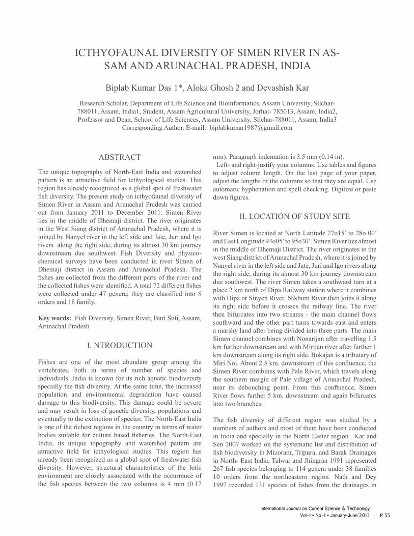
ICTHYOFAUNAL DIVERSITY OF SIMEN RIVER IN AS-SAM AND ARUNACHAL PRADESH, INDIA
Biplab Kumar Das 1*, Aloka Ghosh 2 and Devashish Kar
Research Scholar, Department of Life Science and Bioinformatics, Assam University, Silchar- 788011, Assam, India1, Student, Assam Agricultural University, Jorhat- 785013, Assam, India2, Professor and Dean, School of Life Sciences, Assam University, Silchar-788011, Assam, India3
Corresponding Author. E-mail: [email protected]
ABSTRACT
The unique topography of North-East India and watershed pattern is an attractive field for Icthyological studies. This region has already recognized as a global spot of freshwater fish diversity. The present study on icthyofaunal diversity of Simen River in Assam and Arunachal Pradesh was carried out from January 2011 to December 2011. Simen River lies in the middle of Dhemaji district. The river originates in the West Siang district of Arunachal Pradesh, where it is joined by Nanyel river in the left side and Jate, Juri and Igo rivers along the right side, during its almost 30 km journey downstream due southwest. Fish Diversity and physico-chemical surveys have been conducted in river Simen of Dhemaji district in Assam and Arunachal Pradesh. The fishes are collected from the different parts of the river and the collected fishes were identified. A total 72 different fishes were collected under 47 genera; they are classified into 8 orders and 18 family.
Key words: Fish Diversity, Simen River, Buri Suti, Assam, Arunachal Pradesh
I. NTRODUCTION
Fishes are one of the most abundant group among the vertebrates, both in terms of number of species and individuals. India is known for its rich aquatic biodiversity specially the fish diversity. At the same time, the increased population and environmental degradation have caused damage to this biodiversity. This damage could be severe and may result in loss of genetic diversity, populations and eventually to the extinction of species. The North-East India is one of the richest regions in the country in terms of water bodies suitable for culture based fisheries. The North-East India, its unique topography and watershed pattern are attractive field for icthyological studies. This region has already been recognized as a global spot of freshwater fish diversity. However, structural characteristics of the lotic environment are closely associated with the occurrence of the fish species between the two columns is 4 mm (0.17
mm). Paragraph indentation is 3.5 mm (0.14 in). Left- and right-justify your columns. Use tables and figures to adjust column length. On the last page of your paper, adjust the lengths of the columns so that they are equal. Use automatic hyphenation and spell checking. Digitize or paste down figures.
II. LOCATION OF STUDY SITE
River Simen is located at North Latitude 27o15’ to 28o 00’ and East Longitude 94o05’ to 95o30’. Simen River lies almost in the middle of Dhemaji District. The river originates in the west Siang district of Arunachal Pradesh, where it is joined by Nanyel river in the left side and Jatë, Juri and Igo rivers along the right side, during its almost 30 km journey downstream due southwest. The river Simen takes a southward turn at a place 2 km north of Dipa Railway station where it combines with Dipa or Sinyen River. Nikbum River then joins it along its right side before it crosses the railway line. The river then bifurcates into two streams - the main channel flows southward and the other part turns towards east and enters a marshy land after being divided into three parts. The main Simen channel combines with Nonarijan after travelling 1.5 km further downstream and with Mirijan river after further 1 km downstream along its right side. Bokajan is a tributary of Miri Noi. About 2.5 km. downstream of this confluence, the Simen River combines with Pale River, which travels along the southern margin of Pale village of Arunachal Pradesh, near its debouching point. From this confluence, Simen River flows further 5 km. downstream and again bifurcates into two branches.
The fish diversity of different region was studied by a numbers of authors and most of them have been conducted in India and specially in the North Easter region.. Kar and Sen 2007 worked on the systematic list and distribution of fish biodiversity in Mizoram, Tripura, and Barak Drainages in North- East India. Talwar and Jhingran 1991 represented 267 fish species belonging to 114 genera under 38 families 10 orders from the northeastern region. Nath and Dey 1997 recorded 131 species of fishes from the drainages in
P 55International Journal on Current Science & Technology
Vol - I l No- I l January-June’2013
Arunachal Pradesh. Jayaram 1999 and 2003 studied the freshwater fishes of Indian region. Sen 2000 reported 806 ichthyospecies inhabiting the freshwaters of India. Kar et al. has a huge contribution on the fish diversity, Kar et al. 2006 studied the fish diversity and conservation aspects in an aquatic ecosystems in northeastern India, this work is being done on the biggest freshwater tectonic lake Sone (area 3458.12 ha. at LSL) in Assam, India. Biswas et al. 2008 studied fish diversity of Brahmaputra river in Assam; they continue their work from 1987 to 2000. The diversity of fishes from the upstream to downstream of the Subansiri river described by Sharma et al. 2008; they found there 137 fish species which of them are belonging to the different 7 types of order. Binky and Kar 2011 studied on the icthyospecies diversity in Karbhala wetland of Cachar district of Assam. Das and Kar in 2011 studied the Spatial analysis, Habitat mapping of Subansiri river in the winter season in Assam and Arunachal Pradesh (India). They reported 48 fish species of 15 families under 7 different orders.
III. MATERIALS AND METHODS
Fish samples were collected through experimental fishing using caste nets, gill nets, drag nets, triangular scoop nets and a variety of traps and also by hooks and lines. Fish species have been preserved at first in concentrated (100%) formaldehyde in the field itself in a container and then in 30 % formalin in a glass container. In the laboratory the fish species have been identified after standard literature by following Jayaram (2010), Kar (2007).
IV. RESULTS AND DISCUSSION
Water shows seasonal variation in color. It may be due to the effluents of part time paddy fields and the ingredients of rain water. For most cold water fish, the immune response is severely inhibited below 12oC. Even when water temperatures start to rise there is a time lag of a week or so before the fish immune system starts to function effectively.
The details of fish species recorded from the present study site are given in Table 1. The fish nomenclature is based on Fishbase.org and Jayaram (2010). The present survey of river Simen reveals the presence of 72 (seventy two) species of fishes belonging to 8 (eight) orders, 118 (eighteen) families and 47 (forty seven) genera. Cypriniformes dominates the whole river and found in higher numbers and Beloniformes and Tetradontiformes are found in less number.
The regular flow of water was diminished to a very minimum level which causes the lowering of the ground water level
resulting to loss of vegetation. The drying up of the river will initiate human activities on the river. The existing fish community comprising of terrestrial as well as aquatic and other organism will face the problems of loss of habitat, feeding sites and breeding grounds as a result of change of vegetation pattern due to change of normal water regime of the river.
Species richness in a region is governed by a number of factors which operate at different spatial and temporal scales. Biotic as well as abiotic factors act together in regulating the local species richness. Stream fishes have been used extensively to examine the relative influences of local and regional factors on local species diversity. Regional diversity is said to be more influenced by biogeography processes, thus more recent works seem to emphasize to the importance of scale in determining species diversity. Stream fishes have been used extensively to examine the relative influences of local and regional factors on local species diversity. Regional diversity is said to be more influenced by biogeography processes, thus more recent works seem to emphasize to the importance of scale in determining species diversity.
V. CONCLUSION
As far as fish diversity of the North-Eastern region is concerned, no intensive collection could be done by anyone due to several reasons including difficult terrain, inaccessible locality, and poor communication facilities. Tributaries of the Simen river particularly the hilly headwaters are inhabited by specific fish fauna that need to be explored.
Table I: Physico- Chemical parameters of River Simen.
Sl.No Parameters Upstream Downstream
1 Water Color Clear or Pale Green
Light Copper Red
2 Water temperature 0C 25.7 26.53 pH 6.84 7.55
4 Dissolved Oxygen (mg/L)
9.84 10.52
5 Free Carbon dioxide (mg/L)
8.4 7.1
6 Conductivity (Ω) 98.43 104.6
7 Total Alkalinity (ppm) 109 87.4
Table 1: List of Fish species of Simen River in Assam and Arunachal Pradesh
SL NO NAME OF FISHES ORDER FAMILY
P 56International Journal on Current Science & Technology Vol - I l No- I l January-June’2013
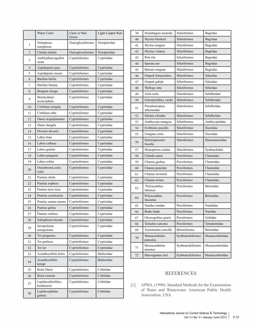
Water Color Clear or Pale Green
Light Copper Red
1 Notopterus notopterus
Osteoglossiformes Notopteridae
2 Chitala chitala Osteoglossiformes Notopteridae
3 Amblypharyngodon mola
Cypriniformes Cyprinidae
4 Aspidopario jaya Cypriniformes Cyprinidae
5 Aspidapario morar Cypriniformes Cyprinidae
6 Barilius barila Cypriniformes Cyprinidae
7 Barilius barana Cypriniformes Cyprinidae
8 Bengala elenga Cypriniformes Cyprinidae
9 Brachydanio aceticephala
Cypriniformes Cyprinidae
10 Cirrhinus mrigala Cypriniformes Cyprinidae
11 Cirrhinus reba Cypriniformes Cyprinidae
12 Danio acquipinnatus Cypriniformes Cyprinidae
13 Danio dangila Cypriniformes Cyprinidae
14 Devario devario Cypriniformes Cyprinidae
15 Labeo bata Cypriniformes Cyprinidae
16 Labeo calbasu Cypriniformes Cyprinidae
17 Labeo gonius Cypriniformes Cyprinidae
18 Labeo pangusia Cypriniformes Cyprinidae
19 Labeo rohita Cypriniformes Cyprinidae
20 Osteobroma cotio cotio
Cypriniformes Cyprinidae
21 Puntius chola Cypriniformes Cyprinidae
22 Puntius sophore Cypriniformes Cyprinidae
23 Puntius ticto ticto Cypriniformes Cyprinidae
24 Puntius conchonius Cypriniformes Cyprinidae
25 Puntius sarana sarana Cypriniformes Cyprinidae
26 Puntius gelius Cypriniformes Cyprinidae
27 Puntius rasbora Cypriniformes Cyprinidae
28 Salmphasia bacaita Cypriniformes Cyprinidae
29 Semipolotus semipolotus
Cypriniformes Cyprinidae
30 Tor progenies Cypriniformes Cyprinidae
31 Tor putitora Cypriniformes Cyprinidae
32 Tor tor Cypriniformes Cyprinidae
33 Acanthocobitis botia Cypriniformes Balitoridae
34 Acanthocobitis kempi
Cypriniformes Balitoridae
35 Botia Dario Cypriniformes Cobitidae
36 Botia rostrata Cypriniformes Cobitidae
37 Lepidocehlichthys berdmorrei
Cypriniformes Cobitidae
38 Lepidocephalus guntea
Cypriniformes Cobitidae
39 Hemibagrus monoda Siluriformes Bagridae
40 Mystus bleekari Siluriformes Bagridae
41 Mystus tengara Siluriformes Bagridae
42 Mystus vittatus Siluriformes Bagridae
43 Rita rita Siluriformes Bagridae
44 Sperata aor Siluriformes Bagridae
45 Batasio tengana Siluriformes Bagridae
46 Ompok bimaculatus Siluriformes Siluridae
47 Ompok pabda Siluriformes Siluridae
48 Wallogo attu Siluriformes Siluridae
49 Ailia coila Siluriformes Schilbeidae
50 Eutropiichthys vacha Siluriformes Schilbeidae
51 Pseudeutropius atherinodes
Siluriformes Schilbeidae
52 Silonia silondia Siluriformes Schilbeidae
53 Amblyceps mangois Siluriformes Amblycipitidae
54 Erethistes pussilis Siluriformes Sisoridae
55 Gangata cenia Siluriformes Sisoridae
56 Heteropneustes fossilis
Siluriformes Heteroneustidae
57 Monopterus cuchia Siluriformes Synbrachidae
58 Chanda nama Perciformes Channidae
59 Channa gachua Perciformes Channidae
60 Channa punctate Perciformes Channidae
61 Channa stewartii Perciformes Channidae
62 Channa striata Perciformes Channidae
63 Polyacanthus labiosus
Perciformes Belonidae
64 Polyacanthus fasciatus
Perciformes Belonidae
65 Nandus nandus Perciformes Nandidae
66 Badis badis Perciformes Nanidae
67 Glossogobius giuris Perciformes Gobidae
68 Tetradon cutcutia Perciformes Tetradontidae
69 Xenentodon cancilla Beloniformes Belonidae
70 Mastacembelus pancalus
Synbranchiformes Mastacembelidae
71 Mastacembelus armatus
Synbranchiformes Mastacembelidae
72 Macrognatus aral Synbranchiformes Mastacembelidae
REFERENCES
[1]. APHA. (1998). Standard Methods for the Examination of Water and Wastewater. American Public Health Association, USA.
P 57International Journal on Current Science & Technology
Vol - I l No- I l January-June’2013
[2] Biswas, B. K. and V. G. Sugnan. (2008). Fish Diversity of Brahmaputra river system in Assam, India. Journal of Inland Fish Sco. India. 40(1): 23-31.
[3] Binky, Kh. and D. Kar. (2011). Ichthyospecies Diversity of Karbhala Wetland in Cachar District of Assam. Environment and Ecology 29 (1): 17-19.
[4] Das, B. K. and D. Kar. (2011). Habitat Mapping, Spatial Analysis of Fish Diversity of River Subansiri during winter season in Assam and Arunachal Pradesh (India). Environment and Ecology 29 (4A): 1948-1951.
[5] Jayaram, K. C. (1999). The freshwater fishes of the Indian region, Narendra Publishing House, Delhi, India. 551 pp.
[6] Jayaram, K. C. (2003). Ecostatus and conservation strategies for Mahaseer fishes of India with special reference to Deccan species. Pp. 3-12. In D. Kar, S. C. Dey and N. C. Dutta (eds). Welfare biology in the new millennium. Pp. xx+97, Allied Publ. Pvt. Ltd., Bangalore, India.
[7] Kar, D. and S. C. Dey. (1987). An account of the Fish and Fisheries of Lake Sone in the Barak Valley of Assam (India). Proceedings of Workshop Development of Beel Fisheries in Assam: 13.
[8] Kar, D. (2000). Present status of fish biodiversity in South Assam and Tripura, 80-82. In: Ponniah, A.G.; Sarker U.K.; (eds). Fish Biodiversity of Northeastern India. NBFGR-NATP Publication No 2, Luckhnow: 228.
[9] Kar, D. (2007). Fundamentals of Limnology and Aquaculture Biotechnology. Daya Publishing House. New Delhi. India. xiv + 609 pp.
[10] Kar, D.; A. V. Nagarathna; T. V. Ramachandra and S. C. Dey. (2006). Fish diversity and conservation aspects in an aquatic ecosystem in northeastern India. Zoos Print J. 21 : 2308-2315.
[11] Kar, D. and N. Sen. (2007). Systematic list and distribution of fish biodiversity in Mizoram, Tripura and Barak drainage in North East India. Zoos print Journal 22(3): 2599-2607.
[12] Nath, P. and S. C. Dey. (1997). Fish and Fisheries of North Eastern India. Volume I: Arunachal Pradesh : 140.
[13] Sen, N. (2000). Occurrence, Distribution and Status of Diversified Fish Fauna of Northeastern India, pp 31- 48. In: Ponniah A.G.; Sarker U.K. Fish Biodiversity of North-East India. NATP Publication No 2. NBFGR, Lucknow: 228.
[14] Sharma, A. K.; C. Mahanta; J. Kalita; A. K. Bhagwati; S. Kalita; B. P. Duarah; S. P. Biswas and J. N. Sharma. (2008). Downstream Impact Study of the ongoing Subansiri Lower Hydroelectric Power Project. National Hydro Electric Power Corporation Limited.
[15] Talwar, P. K. and A. G. Jhingran. (1991). Inland Fishes or India and Adjacent Countries, Vol I and Vol II. Oxford and IBH Co, Pvt. Ltd, New Delhi, India.
P 58International Journal on Current Science & Technology Vol - I l No- I l January-June’2013
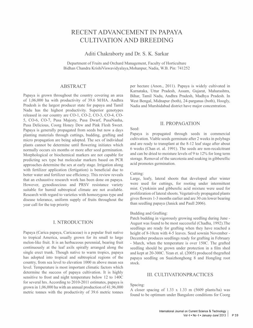
RECENT ADVANCEMENT IN PAPAYACULTIVATION AND BREEDING
ABSTRACT
Papaya is grown throughout the country covering an area of 1,06,000 ha with productivity of 39.6 M/HA. Andhra Pradesh is the largest producer state for papaya and Tamil Nadu has the highest productivity. Superior genotypes released in our country are CO-1, CO-2, CO-3, CO-4, CO-5, CO-6, CO-7, Pusa Majesty, Pusa Dwarf, PusaNanha, Pusa Delicious, Coorg Honey Dew and Pink Flesh Sweet. Papaya is generally propagated from seeds but now a days planting materials through cuttings, budding, grafting and micro propagation are being adopted. The sex of individual plants cannot be determine until flowering initiates which normally occurs six months or more after seed germination. Morphological or biochemical markers are not capable for predicting sex type but molecular markers based on PCR approaches determine the sex at early stage. Irrigation along with fertilizer application (fertigation) is beneficial due to better water and fertilizer use efficiency. This review reveals that an exhaustive research work has been done on papaya. However, gynodioecious and PRSV resistance variety suitable for humid subtropical climate are not available. Research with regard to varieties with homozygous type and disease tolerance, uniform supply of fruits throughout the year call for the top priority
I. NTRODUCTION
Papaya (Carica papaya, Caricaceae) is a popular fruit native to tropical America, usually grown for its small to large melon-like fruit. It is an herbaceous perennial, bearing fruit continuously at the leaf axils spirally arranged along the single erect trunk. Though native to warm tropics, papaya has adopted into tropical and subtropical regions of the country, from sea level to elevation 1000 m above mean sea level. Temperature is most important climatic factors which determine the success of papaya cultivation. It is highly sensitive to frost and night temperature below 12 to 140C for several hrs. According to 2010-2011 estimates, papaya is grown in 1,06,000 ha with an annual production of 41,96,000 metric tonnes with the productivity of 39.6 metric tonnes
Aditi Chakraborty and Dr. S. K. Sarkar
Department of Fruits and Orchard Management, Faculty of HorticultureBidhan Chandra KrishiViswavidyalaya,Mohanpur, Nadia, W.B. Pin: 741252
per hectare (Anon., 2011). Papaya is widely cultivated in Karnataka, Uttar Pradesh, Assam, Gujarat, Maharashtra, Bihar, Tamil Nadu, Andhra Pradesh, Madhya Pradesh. In West Bengal, Midnapur (both), 24-parganas (both), Hoogly, Nadia and Murshidabad district have major concentration.
II. PROPAGATIONSeed:Papaya is propagated through seeds in commercial cultivation. Viable seeds germinate after 2 weeks in polybags and are ready to transplant at the 8-12 leaf stage after about 6 weeks (Chan et. al. 1991). The seeds are non-recalcitrant and can be dried to moisture levels of 9 to 12% for long term storage. Removal of the sarcotesta and soaking in gibberellic acid promotes germination.
Cutting:Large, leafy, lateral shoots that developed after winter were used for cuttings, for rooting under intermittent mist. Cytokinin and gibberelic acid mixture were used for proliferation of lateral shoots. Vegetatively propagated plants gives flowers 1-3 months earlier and are 30 cm lower bearing than seedling papaya (Janick and Paull 2006).
Budding and Grafting:Patch budding in vigorously growing seedling during June - August was found to be most successful (Chadha, 1992).The seedlings are ready for grafting when they have reached a height of 8-10cm with 4-5 leaves. Seed sownin November - December produces seedlings ready for grafting in February - March, when the temperature is over 150C. The grafted seedling should be grown under protection in a film shed and kept at 20-300C. Yean et. al. (2005) produced thegrafted papaya seedling on Suaizhonghong 8 and Hongling root stock.
III. CULTIVATIONPRACTICES
Spacing:A closer spacing of 1.33 x 1.33 m (5609 plants/ha) was found to be optimum under Bangalore conditions for Coorg
P 59International Journal on Current Science & Technology
Vol - I l No- I l January-June’2013
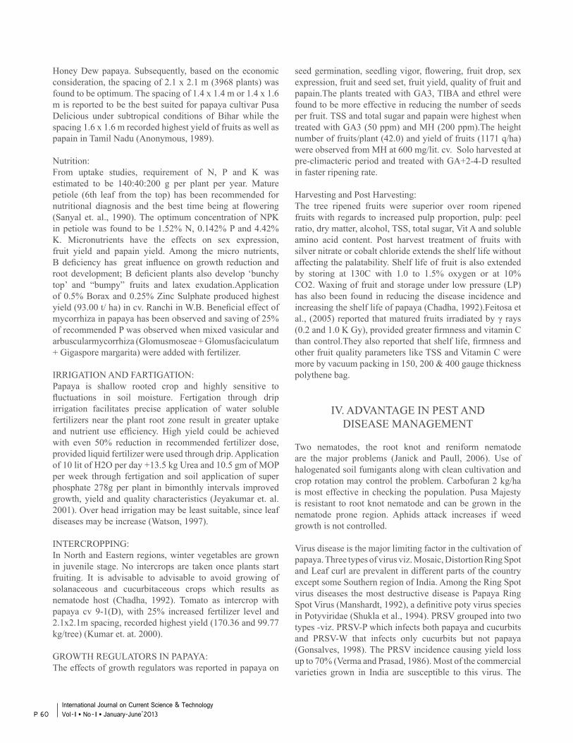
Honey Dew papaya. Subsequently, based on the economic consideration, the spacing of 2.1 x 2.1 m (3968 plants) was found to be optimum. The spacing of 1.4 x 1.4 m or 1.4 x 1.6 m is reported to be the best suited for papaya cultivar Pusa Delicious under subtropical conditions of Bihar while the spacing 1.6 x 1.6 m recorded highest yield of fruits as well as papain in Tamil Nadu (Anonymous, 1989).
Nutrition:From uptake studies, requirement of N, P and K was estimated to be 140:40:200 g per plant per year. Mature petiole (6th leaf from the top) has been recommended for nutritional diagnosis and the best time being at flowering (Sanyal et. al., 1990). The optimum concentration of NPK in petiole was found to be 1.52% N, 0.142% P and 4.42% K. Micronutrients have the effects on sex expression, fruit yield and papain yield. Among the micro nutrients, B deficiency has great influence on growth reduction and root development; B deficient plants also develop ‘bunchy top’ and “bumpy” fruits and latex exudation.Application of 0.5% Borax and 0.25% Zinc Sulphate produced highest yield (93.00 t/ ha) in cv. Ranchi in W.B. Beneficial effect of mycorrhiza in papaya has been observed and saving of 25% of recommended P was observed when mixed vasicular and arbuscularmycorrhiza (Glomusmoseae + Glomusfaciculatum + Gigaspore margarita) were added with fertilizer.
IRRIGATION AND FARTIGATION:Papaya is shallow rooted crop and highly sensitive to fluctuations in soil moisture. Fertigation through drip irrigation facilitates precise application of water soluble fertilizers near the plant root zone result in greater uptake and nutrient use efficiency. High yield could be achieved with even 50% reduction in recommended fertilizer dose, provided liquid fertilizer were used through drip. Application of 10 lit of H2O per day +13.5 kg Urea and 10.5 gm of MOP per week through fertigation and soil application of super phosphate 278g per plant in bimonthly intervals improved growth, yield and quality characteristics (Jeyakumar et. al. 2001). Over head irrigation may be least suitable, since leaf diseases may be increase (Watson, 1997).
INTERCROPPING:In North and Eastern regions, winter vegetables are grown in juvenile stage. No intercrops are taken once plants start fruiting. It is advisable to advisable to avoid growing of solanaceous and cucurbitaceous crops which results as nematode host (Chadha, 1992). Tomato as intercrop with papaya cv 9-1(D), with 25% increased fertilizer level and 2.1x2.1m spacing, recorded highest yield (170.36 and 99.77 kg/tree) (Kumar et. at. 2000).
GROWTH REGULATORS IN PAPAYA:The effects of growth regulators was reported in papaya on
seed germination, seedling vigor, flowering, fruit drop, sex expression, fruit and seed set, fruit yield, quality of fruit and papain.The plants treated with GA3, TIBA and ethrel were found to be more effective in reducing the number of seeds per fruit. TSS and total sugar and papain were highest when treated with GA3 (50 ppm) and MH (200 ppm).The height number of fruits/plant (42.0) and yield of fruits (1171 q/ha) were observed from MH at 600 mg/lit. cv. Solo harvested at pre-climacteric period and treated with GA+2-4-D resulted in faster ripening rate.
Harvesting and Post Harvesting:The tree ripened fruits were superior over room ripened fruits with regards to increased pulp proportion, pulp: peel ratio, dry matter, alcohol, TSS, total sugar, Vit A and soluble amino acid content. Post harvest treatment of fruits with silver nitrate or cobalt chloride extends the shelf life without affecting the palatability. Shelf life of fruit is also extended by storing at 130C with 1.0 to 1.5% oxygen or at 10% CO2. Waxing of fruit and storage under low pressure (LP) has also been found in reducing the disease incidence and increasing the shelf life of papaya (Chadha, 1992).Feitosa et al., (2005) reported that matured fruits irradiated by γ rays (0.2 and 1.0 K Gy), provided greater firmness and vitamin C than control.They also reported that shelf life, firmness and other fruit quality parameters like TSS and Vitamin C were more by vacuum packing in 150, 200 & 400 gauge thickness polythene bag.
IV. ADVANTAGE IN PEST ANDDISEASE MANAGEMENT
Two nematodes, the root knot and reniform nematode are the major problems (Janick and Paull, 2006). Use of halogenated soil fumigants along with clean cultivation and crop rotation may control the problem. Carbofuran 2 kg/ha is most effective in checking the population. Pusa Majesty is resistant to root knot nematode and can be grown in the nematode prone region. Aphids attack increases if weed growth is not controlled.
Virus disease is the major limiting factor in the cultivation of papaya. Three types of virus viz. Mosaic, Distortion Ring Spot and Leaf curl are prevalent in different parts of the country except some Southern region of India. Among the Ring Spot virus diseases the most destructive disease is Papaya Ring Spot Virus (Manshardt, 1992), a definitive poty virus species in Potyviridae (Shukla et al., 1994). PRSV grouped into two types -viz. PRSV-P which infects both papaya and cucurbits and PRSV-W that infects only cucurbits but not papaya (Gonsalves, 1998). The PRSV incidence causing yield loss up to 70% (Verma and Prasad, 1986). Most of the commercial varieties grown in India are susceptible to this virus. The
P 60International Journal on Current Science & Technology Vol - I l No- I l January-June’2013
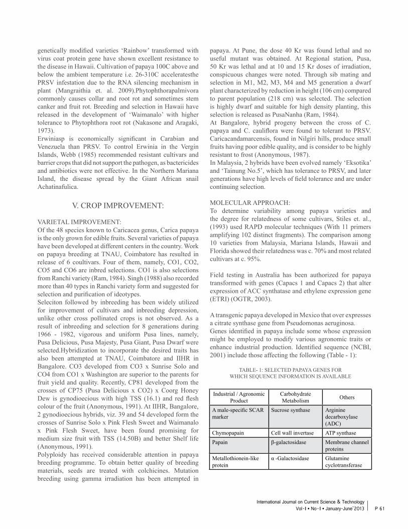
genetically modified varieties ‘Rainbow’ transformed with virus coat protein gene have shown excellent resistance to the disease in Hawaii. Cultivation of papaya 100C above and below the ambient temperature i.e. 26-310C acceleratesthe PRSV infestation due to the RNA silencing mechanism in plant (Mangraithia et. al. 2009).Phytophthorapalmivora commonly causes collar and root rot and sometimes stem canker and fruit rot. Breeding and selection in Hawaii have released in the development of ‘Waimanalo’ with higher tolerance to Phytophthora root rot (Nakasone and Aragaki, 1973). Erwiniasp is economically significant in Carabian and Venezuela than PRSV. To control Erwinia in the Vergin Islands, Webb (1985) recommended resistant cultivars and barrier crops that did not support the pathogen, as bactericides and antibiotics were not effective. In the Northern Mariana Island, the disease spread by the Giant African snail Achatinafulica.
V. CROP IMPROVEMENT:
VARIETAL IMPROVEMENT:Of the 48 species known to Caricacea genus, Carica papaya is the only grown for edible fruits. Several varieties of papaya have been developed at different centers in the country. Work on papaya breeding at TNAU, Coimbatore has resulted in release of 6 coultivars. Four of them, namely, CO1, CO2, CO5 and CO6 are inbred selections. CO1 is also selections from Ranchi variety (Ram, 1984). Singh (1988) also recorded more than 40 types in Ranchi variety form and suggested for selection and purification of ideotypes.Seleciton followed by inbreeding has been widely utilized for improvement of cultivars and inbreeding depression, unlike other cross pollinated crops is not observed. As a result of inbreeding and selection for 8 generations during 1966 - 1982, vigorous and uniform Pusa lines, namely, Pusa Delicious, Pusa Majesty, Pusa Giant, Pusa Dwarf were selected.Hybridization to incorporate the desired traits has also been attempted at TNAU, Coimbatore and IIHR in Bangalore. CO3 developed from CO3 x Sunrise Solo and CO4 from CO1 x Washington are superior to the parents for fruit yield and quality. Recently, CP81 developed from the crosses of CP75 (Pusa Delicious x CO2) x Coorg Honey Dew is gynodioecious with high TSS (16.1) and red flesh colour of the fruit (Anonymous, 1991). At IIHR, Bangalore, 2 gynodioecious hybrids, viz. 39 and 54 developed form the crosses of Sunrise Solo x Pink Flesh Sweet and Waimanalo x Pink Flesh Sweet, have been found promising for medium size fruit with TSS (14.50B) and better Shelf life (Anonymous, 1991).Polyploidy has received considerable attention in papaya breeding programme. To obtain better quality of breeding materials, seeds are treated with colchicines. Mutation breeding using gamma irradiation has been attempted in
papaya. At Pune, the dose 40 Kr was found lethal and no useful mutant was obtained. At Regional station, Pusa, 50 Kr was lethal and at 10 and 15 Kr doses of irradiation, conspicuous changes were noted. Through sib mating and selection in M1, M2, M3, M4 and M5 generation a dwarf plant characterized by reduction in height (106 cm) compared to parent population (218 cm) was selected. The selection is highly dwarf and suitable for high density planting, this selection is released as PusaNanha (Ram, 1984).At Bangalore, hybrid progeny between the cross of C. papaya and C. cauliflora were found to tolerant to PRSV. Caricacandamarcensis, found in Nilgiri hills, produce small fruits having poor edible quality, and is consider to be highly resistant to frost (Anonymous, 1987).In Malaysia, 2 hybrids have been evolved namely ‘Eksotika’ and ‘Tainung No.5’, which has tolerance to PRSV, and later generations have high levels of field tolerance and are under continuing selection.
MOLECULAR APPROACH:To determine variability among papaya varieties and the degree for relatedness of some cultivars, Stiles et. al., (1993) used RAPD molecular techniques (With 11 primers amplifying 102 distinct fragments). The comparison among 10 varieties from Malaysia, Mariana Islands, Hawaii and Florida showed their relatedness was c. 70% and most related cultivars at c. 95%.
Field testing in Australia has been authorized for papaya transformed with genes (Capacs 1 and Capacs 2) that alter expression of ACC synthatase and ethylene expression gene (ETRI) (OGTR, 2003).
A transgenic papaya developed in Mexico that over expresses a citrate synthase gene from Pseudomonas aeruginosa.Genes identified in papaya include some whose expression might be employed to modify various agronomic traits or enhance industrial production. Identified sequence (NCBI, 2001) include those affecting the following (Table - 1):
TABLE- 1: SELECTED PAPAYA GENES FORWHICH SEQUENCE INFORMATION IS AVAILABLE
Industrial / Agronomic Product
Carbohydrate Metabolism Others
A male-specific SCAR marker
Sucrose synthase Arginine decarboxylase (ADC)
Chymopapain Cell wall invertase ATP synthase Papain β-galactosidase Membrane channel
proteinsMetallothionein-like protein
α -Galactosidase Glutamine cyclotransferase
P 61International Journal on Current Science & Technology
Vol - I l No- I l January-June’2013
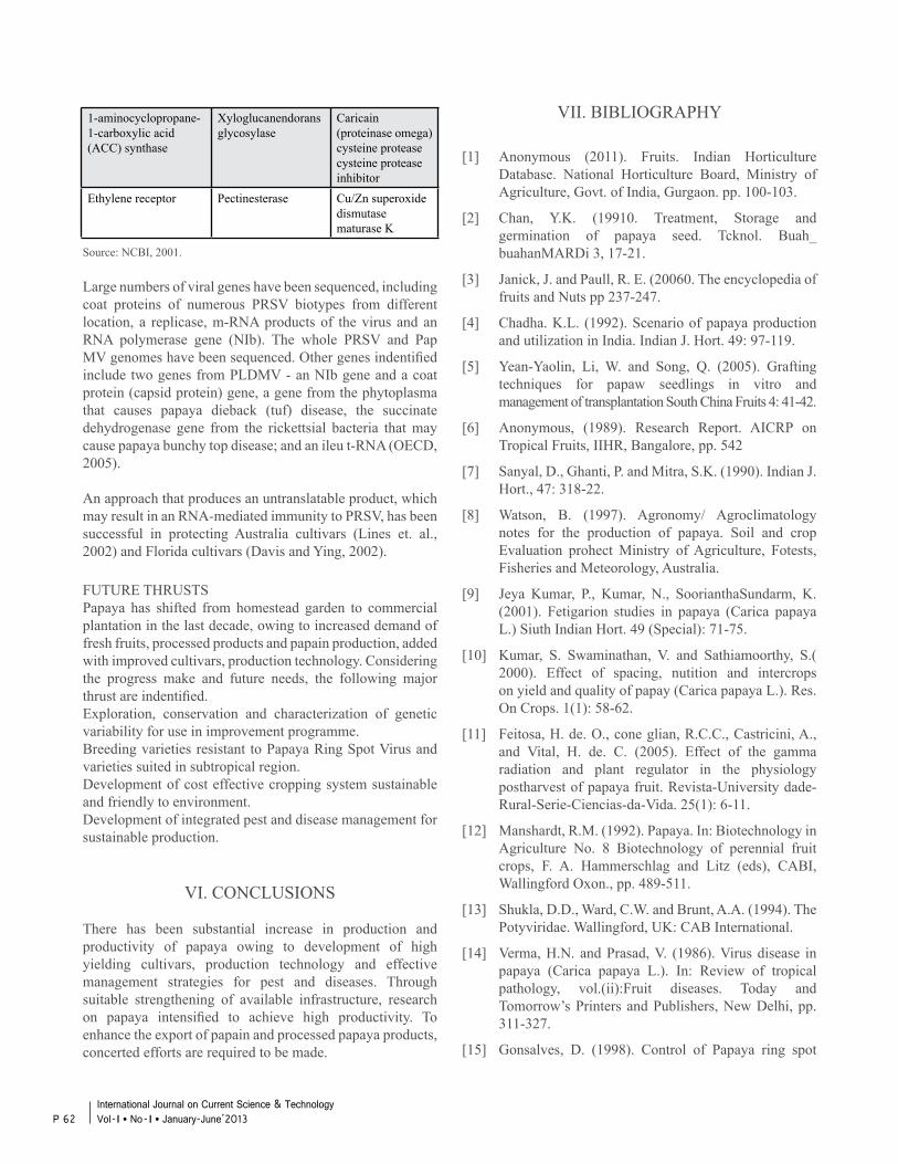
1-aminocyclopropane-1-carboxylic acid (ACC) synthase
Xyloglucanendorans glycosylase
Caricain (proteinase omega) cysteine protease cysteine protease inhibitor
Ethylene receptor Pectinesterase Cu/Zn superoxide dismutase maturase K
Source: NCBI, 2001.
Large numbers of viral genes have been sequenced, including coat proteins of numerous PRSV biotypes from different location, a replicase, m-RNA products of the virus and an RNA polymerase gene (NIb). The whole PRSV and Pap MV genomes have been sequenced. Other genes indentified include two genes from PLDMV - an NIb gene and a coat protein (capsid protein) gene, a gene from the phytoplasma that causes papaya dieback (tuf) disease, the succinate dehydrogenase gene from the rickettsial bacteria that may cause papaya bunchy top disease; and an ileu t-RNA (OECD, 2005).
An approach that produces an untranslatable product, which may result in an RNA-mediated immunity to PRSV, has been successful in protecting Australia cultivars (Lines et. al., 2002) and Florida cultivars (Davis and Ying, 2002).
FUTURE THRUSTSPapaya has shifted from homestead garden to commercial plantation in the last decade, owing to increased demand of fresh fruits, processed products and papain production, added with improved cultivars, production technology. Considering the progress make and future needs, the following major thrust are indentified.Exploration, conservation and characterization of genetic variability for use in improvement programme.Breeding varieties resistant to Papaya Ring Spot Virus and varieties suited in subtropical region.Development of cost effective cropping system sustainable and friendly to environment.Development of integrated pest and disease management for sustainable production.
VI. CONCLUSIONS
There has been substantial increase in production and productivity of papaya owing to development of high yielding cultivars, production technology and effective management strategies for pest and diseases. Through suitable strengthening of available infrastructure, research on papaya intensified to achieve high productivity. To enhance the export of papain and processed papaya products, concerted efforts are required to be made.
VII. BIBLIOGRAPHY
[1] Anonymous (2011). Fruits. Indian Horticulture Database. National Horticulture Board, Ministry of Agriculture, Govt. of India, Gurgaon. pp. 100-103.
[2] Chan, Y.K. (19910. Treatment, Storage and germination of papaya seed. Tcknol. Buah_ buahanMARDi 3, 17-21.
[3] Janick, J. and Paull, R. E. (20060. The encyclopedia of fruits and Nuts pp 237-247.
[4] Chadha. K.L. (1992). Scenario of papaya production and utilization in India. Indian J. Hort. 49: 97-119.
[5] Yean-Yaolin, Li, W. and Song, Q. (2005). Grafting techniques for papaw seedlings in vitro and management of transplantation South China Fruits 4: 41-42.
[6] Anonymous, (1989). Research Report. AICRP on Tropical Fruits, IIHR, Bangalore, pp. 542
[7] Sanyal, D., Ghanti, P. and Mitra, S.K. (1990). Indian J. Hort., 47: 318-22.
[8] Watson, B. (1997). Agronomy/ Agroclimatology notes for the production of papaya. Soil and crop Evaluation prohect Ministry of Agriculture, Fotests, Fisheries and Meteorology, Australia.
[9] Jeya Kumar, P., Kumar, N., SoorianthaSundarm, K. (2001). Fetigarion studies in papaya (Carica papaya L.) Siuth Indian Hort. 49 (Special): 71-75.
[10] Kumar, S. Swaminathan, V. and Sathiamoorthy, S.( 2000). Effect of spacing, nutition and intercrops on yield and quality of papay (Carica papaya L.). Res. On Crops. 1(1): 58-62.
[11] Feitosa, H. de. O., cone glian, R.C.C., Castricini, A., and Vital, H. de. C. (2005). Effect of the gamma radiation and plant regulator in the physiology postharvest of papaya fruit. Revista-University dade- Rural-Serie-Ciencias-da-Vida. 25(1): 6-11.
[12] Manshardt, R.M. (1992). Papaya. In: Biotechnology in Agriculture No. 8 Biotechnology of perennial fruit crops, F. A. Hammerschlag and Litz (eds), CABI, Wallingford Oxon., pp. 489-511.
[13] Shukla, D.D., Ward, C.W. and Brunt, A.A. (1994). The Potyviridae. Wallingford, UK: CAB International.
[14] Verma, H.N. and Prasad, V. (1986). Virus disease in papaya (Carica papaya L.). In: Review of tropical pathology, vol.(ii):Fruit diseases. Today and Tomorrow’s Printers and Publishers, New Delhi, pp. 311-327.
[15] Gonsalves, D. (1998). Control of Papaya ring spot
P 62International Journal on Current Science & Technology Vol - I l No- I l January-June’2013
virus in papaya: A case study. Ann. Rev. Phytopathol,36: 415-437.
[16] Mangrauthia, S.K., Shakya, V.P.S., Hain, R.K. and Shelly, P. (2009). Ambient temperature perception in papaya for Papaya ringspot virus interaction.
[17] Nakasone, H.Y. and Aragaki, M. (1973). Tolerance to Phytophthora fruit and root rot in Carica papaya. 2 Proc. Of the Tropical Region American Soc. For Hort. Sci. 17: 176 - 185.
[18] Webb, R.R. (1985). Epidemiology and control of bacterial canker of papaya caused by an Erwinia sp. On St. Croix, U.S. Virgin Islands. Plnat Disease 69: 305 - 309.
[19] Ram, M. (1984). Promising varieties of papaya. In: Proc. Papaya and papain production seminar, Coimbatore, India 26-27 March. pp. 37-39.
[20] Singh, H.R. (1988). In National Convention on strategies of horticultural development for tribal region, Ranchi, pp. 8
[21] Anonymous, (1991) research report. AICRP on Tropical Fruit, IIHR, Bangalore. pp. 454.
[22] Anonymous, (1987). Rresearch Report AIARP on Tropical Rruits. IIHR, Bangalore. pp. 450
[23] Stiles, H.I., Lemme, C., Sondur, M.B. and Manshardt, R.(1993). Using Randomly amplified polymorphic DNA for evaluating relationships among papaya cultivars. Theor. Appl. Genetics 85: 697 - 701.
[24] OGTR (2003). Risk Assessment and Risk Management Plan. Application for License for Dealings Involving an Intentional Release into the Environment. DIR 026/2006. June 2003. Office of the Gene Technology Regulator, Government of Australia. http://www.ogtr. gob.au/ir/dir026.htm
[25] NCBI (2001). NCBI Gen Bank (nucleotide database). http://www.ncbi.nlm.nih.gov
[26] Organiastion of Economic co-operation and Development (OECD), paris. Consensus document on the biology of papaya (Carica papaya). 2005(16). Pp- 5-64. http://www.oecd.org/ehs/
[27] Lines, R.E., Persley, D., Dale, J.L., Drew, R and Bateson, M.F. (2002). Genetically engineered immunity to papaya ringspot virus in Australian cultivars. Molec. Breed. 10: 119 - 129.
[28] Davis, M.J., and Z. Ying. (2002). Development of transgenic ringspot virus resistant papaya for Florida. Phytopathology 92 (6, Suppl.): S 18.
P 63International Journal on Current Science & Technology
Vol - I l No- I l January-June’2013

P 64International Journal on Current Science & Technology Vol - I l No- I l January-June’2013
TRADITIONAL ORGANIC PRACTICES WITH TRADITIONAL INPUTS FARMING FOR THE
CULTIVATION OF FRENCH BEAN IN MANIPUR
G.K.N.Chhetry and H.C.Mangang
Department of Life Sciences, Manipur University, Canchipur, Imphal- 795003.
ABSTRACT
Traditional farming practices are an important source of knowledge for sustainable agriculture being practiced by diverse communities of the region and are much akin to the modern organic farming system. Hence a study of the various farming practices of the farming communities and their documentation assumed significance to safeguard the rich heritage of the traditional farmers for the sustainability of organic crop production system. Home garden is one such agricultural system maintained organically for a perennial source of vegetables. It has been observed that most of the farming practices of the marginal farmers in the home gardens were organic in nature. Utilization of all sorts of organic litters produced in the farms and households either as composted or partially composted form were organic sources of manures. Decrease trend of organic home garden in sizes of house holdings for home gardens was found due to the urbanization process. Organic manures produced in the households and farms were sufficient for the small landholdings and for the growth of less fertiliser intensive crop like french bean. Recycling of organic waste of kitchen and farm yard in the organic management of french bean crop and documentation of traditional practices are the key issue of this paper.
I. NTRODUCTION
Organic farming system is a system where different components directly or indirectly influence the production system without the synthetic chemical components as used in modern agriculture. In other words, organic farming system is free from all kinds of synthetic chemicals viz. hormones, genetically modified crops etc. Organic farming is in fact a kind of natural farming system evolved by the indigenous farming communities since time immemorial and still in practice in different parts of the world mostly in the developing countries where modern high tech farming facilities are either not accessible or rejected by the indigenous communities in view of its hazardous effect on
environment and loss of genetic diversity of traditional crops. In India before the launch of green revolution to enhance the agricultural output in order to cope with the population explosion, organic farming system was the only option for the production of crops for healthy life style of the people. Influence of green revolution was limited to plain and high tech assessable agricultural land only and therefore far flung hill areas of the country could not become beneficiary of the green revolution, either due to inaccessibility of the same. Farming communities of the North Eastern region
of India prefer to follow the traditional organic farming system as they have been doing since generation in the form of Jhum cultivation and organic home gardening. As such traditional farming systems and its practices is still prevailing in remote areas particularly in the hill states as for example, in the North Eastern states of India where more than 150 ethnic groups are practicing organic farming system with slight variations in location specific organic farming systems. Balasubramanian (2006) advocated the need to safeguard the traditional practices to prevent from the clutches of western influence. Rationale of the Indigenous knowledge and their documentation in part was carried out by Pulmate and Babu (1993) ,Chhetry and Belbahri (2009) in Manipur. However, the basic information of the system such as organic farms and its types regarding its house holding size, preparation of organic manures and their application procedures in respect of crop like french bean in particular followed by different ethnic communities have not been fully documented either by traditional communities or by scientific communities in this part of the country where french bean is mostly grown as home garden crop for domestic consumption. Importance of documentation of different components of organic farming system in view of the reducing trend of practicing organic farming system by the indigenous farming community due to heavy influence of modern agriculture for the greed of bumper production to meet the food requirement of growing population is tremendrous. As such extensive survey work both location specific site and roaming site concerning hills and plains of Manipur was carried out to assess the organic practices followed by indigenous farmers for the
P 65International Journal on Current Science & Technology
Vol - I l No- I l January-June’2013
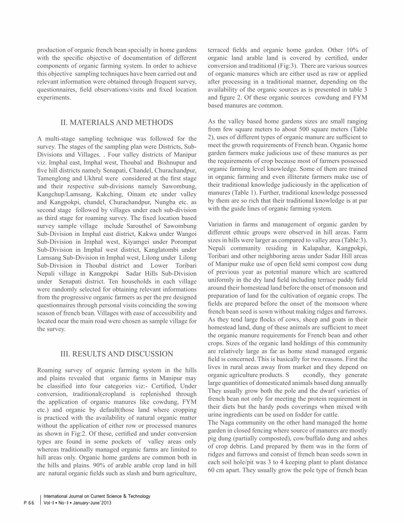
production of organic french bean specially in home gardens with the specific objective of documentation of different components of organic farming system. In order to achieve this objective sampling techniques have been carried out and relevant information were obtained through frequent survey, questionnaires, field observations/visits and fixed location experiments.
II. MATERIALS AND METHODS
A multi-stage sampling technique was followed for the survey. The stages of the sampling plan were Districts, Sub-Divisions and Villages. . Four valley districts of Manipur viz. Imphal east, Imphal west, Thoubal and Bishnupur and five hill districts namely Senapati, Chandel, Churachandpur, Tamenglong and Ukhrul were considered at the first stage and their respective sub-divisions namely Sawombung, Kangchup/Lamsang, Kakching, Oinam etc under valley and Kangpokpi, chandel, Churachandpur, Nungba etc. as second stage followed by villages under each sub-division as third stage for roaming survey. The fixed location based survey sample village include Sarouthel of Sawombung Sub-Division in Imphal east district, Kakwa under Wangoi Sub-Division in Imphal west, Kiyamgei under Porompat Sub-Division in Imphal west district, Kanglatombi under Lamsang Sub-Division in Imphal west, Lilong under Lilong Sub-Division in Thoubal district and Lower Toribari Nepali village in Kangpokpi Sadar Hills Sub-Division under Senapati district. Ten households in each village were randomly selected for obtaining relevant informations from the progressive organic farmers as per the pre designed questionnaires through personal visits coinciding the sowing season of french bean. Villages with ease of accessibility and located near the main road were chosen as sample village for the survey.
III. RESULTS AND DISCUSSION
Roaming survey of organic farming system in the hills and plains revealed that organic farms in Manipur may be classified into four categories viz:- Certified, Under conversion, traditional(cropland is replenished through the application of organic manures like cowdung, FYM etc.) and organic by default(those land where cropping is practiced with the availability of natural organic matter without the application of either row or processed manures as shown in Fig:2. Of these, certified and under conversion types are found in some pockets of valley areas only whereas traditionally managed organic farms are limited to hill areas only. Organic home gardens are common both in the hills and plains. 90% of arable arable crop land in hill are natural organic fields such as slash and burn agriculture,
terraced fields and organic home garden. Other 10% of organic land arable land is covered by certified, under conversion and traditional (Fig:3). There are various sources of organic manures which are either used as raw or applied after processing in a traditional manner, depending on the availability of the organic sources as is presented in table 3 and figure 2. Of these organic sources cowdung and FYM based manures are common.
As the valley based home gardens sizes are small ranging from few square meters to about 500 square meters (Table 2), uses of different types of organic manure are sufficient to meet the growth requirements of French bean. Organic home garden farmers make judicious use of these manures as per the requirements of crop because most of farmers possessed organic farming level knowledge. Some of them are trained in organic farming and even illiterate farmers make use of their traditional knowledge judiciously in the application of manures (Table 1). Further, traditional knowledge possessed by them are so rich that their traditional knowledge is at par with the guide lines of organic farming system.
Variation in farms and management of organic garden by different ethnic groups were observed in hill areas. Farm sizes in hills were larger as compared to valley area (Table:3). Nepali community residing in Kalapahar, Kangpokpi, Toribari and other neighboring areas under Sadar Hill areas of Manipur make use of open field semi compost cow dung of previous year as potential manure which are scattered uniformly in the dry land field including terrace paddy field around their homestead land before the onset of monsoon and preparation of land for the cultivation of organic crops. The fields are prepared before the onset of the monsoon where french bean seed is sown without making ridges and furrows. As they tend large flocks of cows, sheep and goats in their homestead land, dung of these animals are sufficient to meet the organic manure requirements for French bean and other crops. Sizes of the organic land holdings of this community are relatively large as far as home stead managed organic field is concerned. This is basically for two reasons. First the lives in rural areas away from market and they depend on organic agriculture products. S econdly, they generate large quantities of domesticated animals based dung annually They usually grow both the pole and the dwarf varieties of french bean not only for meeting the protein requirement in their diets but the hardy pods coverings when mixed with urine ingredients can be used on fodder for cattle.The Naga community on the other hand managed the home garden in closed fencing where source of manures are mostly pig dung (partially composted), cow/buffalo dung and ashes of crop debris. Land prepared by them was in the form of ridges and furrows and consist of french bean seeds sown in each soil hole/pit was 3 to 4 keeping plant to plant distance 60 cm apart. They usually grow the pole type of french bean
P 66International Journal on Current Science & Technology Vol - I l No- I l January-June’2013
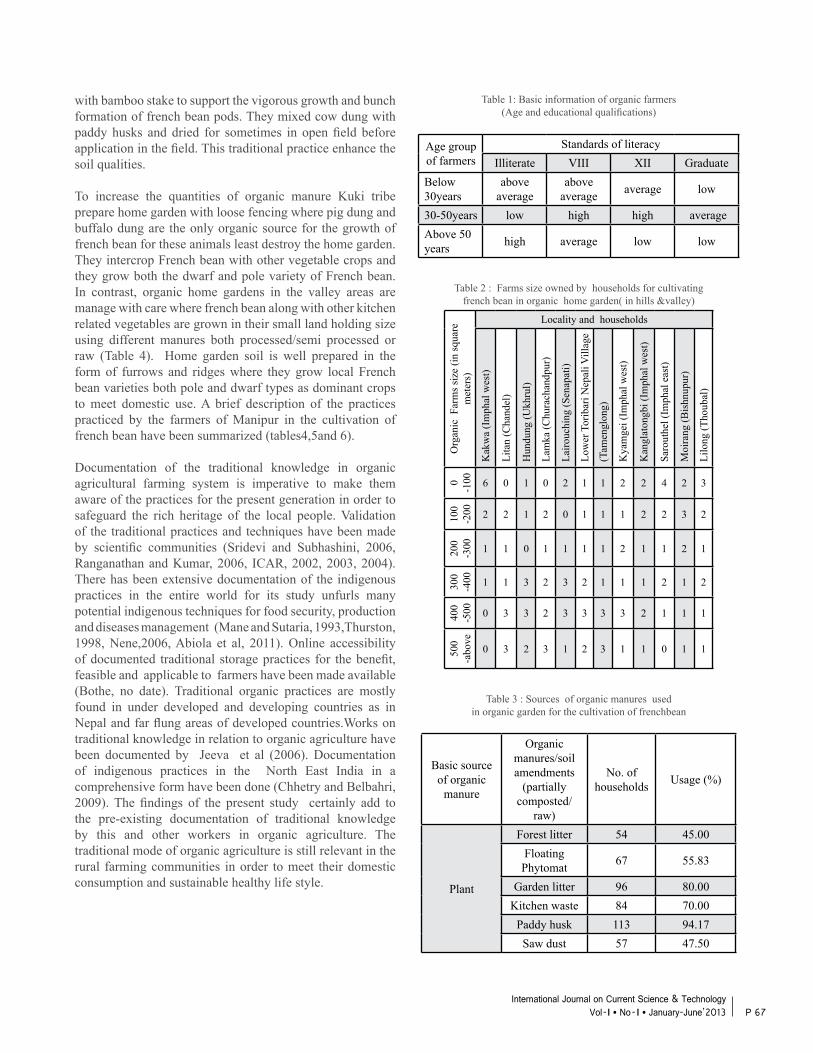
with bamboo stake to support the vigorous growth and bunch formation of french bean pods. They mixed cow dung with paddy husks and dried for sometimes in open field before application in the field. This traditional practice enhance the soil qualities.
To increase the quantities of organic manure Kuki tribe prepare home garden with loose fencing where pig dung and buffalo dung are the only organic source for the growth of french bean for these animals least destroy the home garden. They intercrop French bean with other vegetable crops and they grow both the dwarf and pole variety of French bean. In contrast, organic home gardens in the valley areas are manage with care where french bean along with other kitchen related vegetables are grown in their small land holding size using different manures both processed/semi processed or raw (Table 4). Home garden soil is well prepared in the form of furrows and ridges where they grow local French bean varieties both pole and dwarf types as dominant crops to meet domestic use. A brief description of the practices practiced by the farmers of Manipur in the cultivation of french bean have been summarized (tables4,5and 6).
Documentation of the traditional knowledge in organic agricultural farming system is imperative to make them aware of the practices for the present generation in order to safeguard the rich heritage of the local people. Validation of the traditional practices and techniques have been made by scientific communities (Sridevi and Subhashini, 2006, Ranganathan and Kumar, 2006, ICAR, 2002, 2003, 2004).There has been extensive documentation of the indigenous practices in the entire world for its study unfurls many potential indigenous techniques for food security, production and diseases management (Mane and Sutaria, 1993,Thurston, 1998, Nene,2006, Abiola et al, 2011). Online accessibility of documented traditional storage practices for the benefit, feasible and applicable to farmers have been made available (Bothe, no date). Traditional organic practices are mostly found in under developed and developing countries as in Nepal and far flung areas of developed countries.Works on traditional knowledge in relation to organic agriculture have been documented by Jeeva et al (2006). Documentation of indigenous practices in the North East India in a comprehensive form have been done (Chhetry and Belbahri, 2009). The findings of the present study certainly add to the pre-existing documentation of traditional knowledge by this and other workers in organic agriculture. The traditional mode of organic agriculture is still relevant in the rural farming communities in order to meet their domestic consumption and sustainable healthy life style.
Table 1: Basic information of organic farmers(Age and educational qualifications)
Age group of farmers
Standards of literacyIlliterate VIII XII Graduate
Below 30years
above average
above average average low
30-50years low high high averageAbove 50 years high average low low
Table 2 : Farms size owned by households for cultivatingfrench bean in organic home garden( in hills &valley)
Org
anic
Far
ms s
ize
(in sq
uare
m
eter
s)
Locality and households
Kak
wa
(Im
phal
wes
t)
Lita
n (C
hand
el)
Hun
dung
(Ukh
rul)
Lam
ka (C
hura
chan
dpur
)
Lairo
uchi
ng (S
enap
ati)
Low
er T
orib
ari N
epal
i Vill
age
(Tam
engl
ong)
Kya
mge
i (Im
phal
wes
t)
Kan
glat
ongb
i (Im
phal
wes
t)
Saro
uthe
l (Im
phal
eas
t)
Moi
rang
(Bis
hnup
ur)
Lilo
ng (T
houb
al)
0 -1
00 6 0 1 0 2 1 1 2 2 4 2 3
100
-200 2 2 1 2 0 1 1 1 2 2 3 2
200
-300 1 1 0 1 1 1 1 2 1 1 2 1
300
-400 1 1 3 2 3 2 1 1 1 2 1 2
400
-500 0 3 3 2 3 3 3 3 2 1 1 1
500
-abo
ve
0 3 2 3 1 2 3 1 1 0 1 1
Table 3 : Sources of organic manures used in organic garden for the cultivation of frenchbean
Basic source of organic
manure
Organic manures/soil amendments
(partially composted/
raw)
No. of households Usage (%)
Plant
Forest litter 54 45.00Floating Phytomat 67 55.83
Garden litter 96 80.00Kitchen waste 84 70.00
Paddy husk 113 94.17Saw dust 57 47.50
P 67International Journal on Current Science & Technology
Vol - I l No- I l January-June’2013
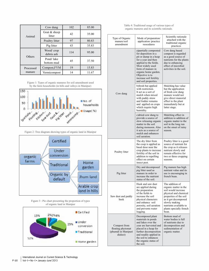
Animal
Cow dung 102 85.00Goat & sheep
litter 42 35.00
Poultry litter 97 80.83Pig litter 43 35.83
Others
Wood/ crop debris ash 114 95.00
Pond/ lake bottom mud 45 37.50
Processed manure
Compost,FYM 19 15.83Vermicompost 14 11.67
Figure 1: Types of organic manures for soil amendment usedby the farm households (in hills and valleys in Manipur)
Figure 2 :Tree diagram showing types of organic land in Manipur
Figure 3 : Pie chart presenting the proportion of typesof organic land in Manipur
Table 4: Traditional usage of various types oforganic manures and its scientific rationale.
Type of Organic manure/soil amendment
Mode of preparation/application /practice
reocedures
Scientific rationale attached with the
traditional organic practices
Cow dung
a)partially composted for deposition in a pit or dump in a heap for a year and then applied to the fields. Most widely used form of manure in organic home garden. Objective is to increase soil fertility and soil properties.
Cow dung based compost is regarded as a good source of nutrients for the plants due to enhancing effect of microbial activities in the soil.
b)fresh but applied with restriction. It act as a sort of mulch when mixed with paddy straw and fodder remains and applied on crops which require high humidity.
Mulching has value but the application of fresh cow dung manure would not give direct manorial effect to the plant immediately but at latter stage.
c)dried cow dung to provide a source of slow releasing organic matter to the soil during monsoon. Also it acts as a source of mulch and enhances soil aeration.
Mulching effect in addition to addition of organic matter to the soil in the long run on the onset of rainy season.
Poultry litter
The dry litter from the coop is applied as basal dose near the crop plants to increase fertility of the soil in addition to repelling effect on certain insect pest.
Poultry litter is a good source of nutrient for the crop as it releases nutrient slowly and remain effective for two or three cropping seasons.
Pig litter
Dry and decomposed pig litter used as manure in order to increase the nutrient status of the soil.
Pig manure has high nutrient value and its use is encouraging in french bean.
Saw dust and paddy husk
Husk and saw dust are applied during the preparation of the fields to increase the soil physical characters and enhance soil porosity, soil aeration and prevents water logging.
The addition of organic matter in the soil would increase physical and chemical properties of the soil as it got decomposed slowly making nutrients available to plants specially french bean.
Compost from floating phytomat
(phumdi in Manipuri dialect)
Decomposed plant materials in ponds and lakes over the year are harvested and placed in a heap for further decomposition and readily applied in the soil to enhances the organic status of the soil.
Bottom mud of water bodies is full of nutrients due to decomposition and sedimentation of organic matter.
P 68International Journal on Current Science & Technology Vol - I l No- I l January-June’2013
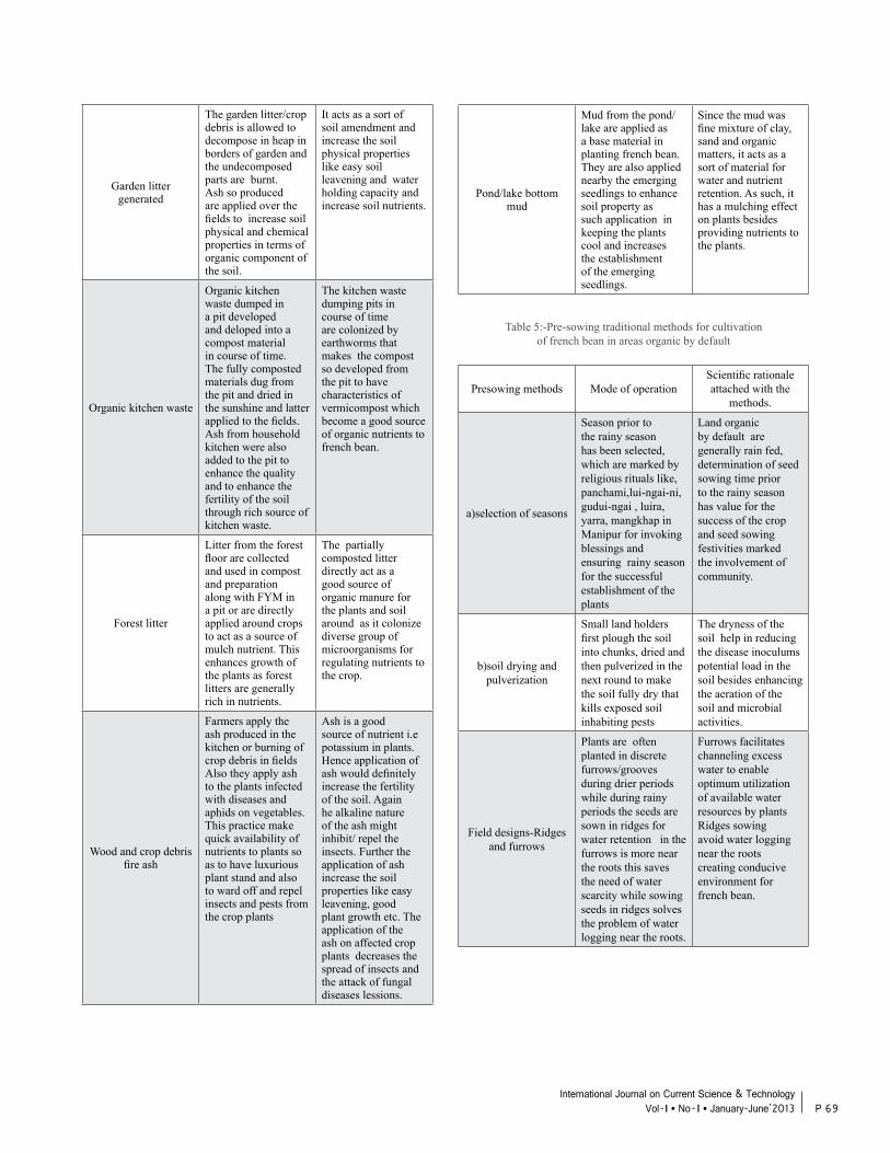
Garden litter generated
The garden litter/crop debris is allowed to decompose in heap in borders of garden and the undecomposed parts are burnt. Ash so produced are applied over the fields to increase soil physical and chemical properties in terms of organic component of the soil.
It acts as a sort of soil amendment and increase the soil physical properties like easy soil leavening and water holding capacity and increase soil nutrients.
Organic kitchen waste
Organic kitchen waste dumped in a pit developed and deloped into a compost material in course of time. The fully composted materials dug from the pit and dried in the sunshine and latter applied to the fields. Ash from household kitchen were also added to the pit to enhance the quality and to enhance the fertility of the soil through rich source of kitchen waste.
The kitchen waste dumping pits in course of time are colonized by earthworms that makes the compost so developed from the pit to have characteristics of vermicompost which become a good source of organic nutrients to french bean.
Forest litter
Litter from the forest floor are collected and used in compost and preparation along with FYM in a pit or are directly applied around crops to act as a source of mulch nutrient. This enhances growth of the plants as forest litters are generally rich in nutrients.
The partially composted litter directly act as a good source of organic manure for the plants and soil around as it colonize diverse group of microorganisms for regulating nutrients to the crop.
Wood and crop debris fire ash
Farmers apply the ash produced in the kitchen or burning of crop debris in fields Also they apply ash to the plants infected with diseases and aphids on vegetables. This practice make quick availability of nutrients to plants so as to have luxurious plant stand and also to ward off and repel insects and pests from the crop plants
Ash is a good source of nutrient i.e potassium in plants. Hence application of ash would definitely increase the fertility of the soil. Again he alkaline nature of the ash might inhibit/ repel the insects. Further the application of ash increase the soil properties like easy leavening, good plant growth etc. The application of the ash on affected crop plants decreases the spread of insects and the attack of fungal diseases lessions.
Pond/lake bottom mud
Mud from the pond/lake are applied as a base material in planting french bean. They are also applied nearby the emerging seedlings to enhance soil property as such application in keeping the plants cool and increases the establishment of the emerging seedlings.
Since the mud was fine mixture of clay, sand and organic matters, it acts as a sort of material for water and nutrient retention. As such, it has a mulching effect on plants besides providing nutrients to the plants.
Table 5:-Pre-sowing traditional methods for cultivationof french bean in areas organic by default
Presowing methods Mode of operation Scientific rationale attached with the
methods.
a)selection of seasons
Season prior to the rainy season has been selected, which are marked by religious rituals like, panchami,lui-ngai-ni, gudui-ngai , luira, yarra, mangkhap in Manipur for invoking blessings and ensuring rainy season for the successful establishment of the plants
Land organic by default are generally rain fed, determination of seed sowing time prior to the rainy season has value for the success of the crop and seed sowing festivities marked the involvement of community.
b)soil drying and pulverization
Small land holders first plough the soil into chunks, dried and then pulverized in the next round to make the soil fully dry that kills exposed soil inhabiting pests
The dryness of the soil help in reducing the disease inoculums potential load in the soil besides enhancing the aeration of the soil and microbial activities.
Field designs-Ridges and furrows
Plants are often planted in discrete furrows/grooves during drier periods while during rainy periods the seeds are sown in ridges for water retention in the furrows is more near the roots this saves the need of water scarcity while sowing seeds in ridges solves the problem of water logging near the roots.
Furrows facilitates channeling excess water to enable optimum utilization of available water resources by plants Ridges sowing avoid water logging near the roots creating conducive environment for french bean.
P 69International Journal on Current Science & Technology
Vol - I l No- I l January-June’2013
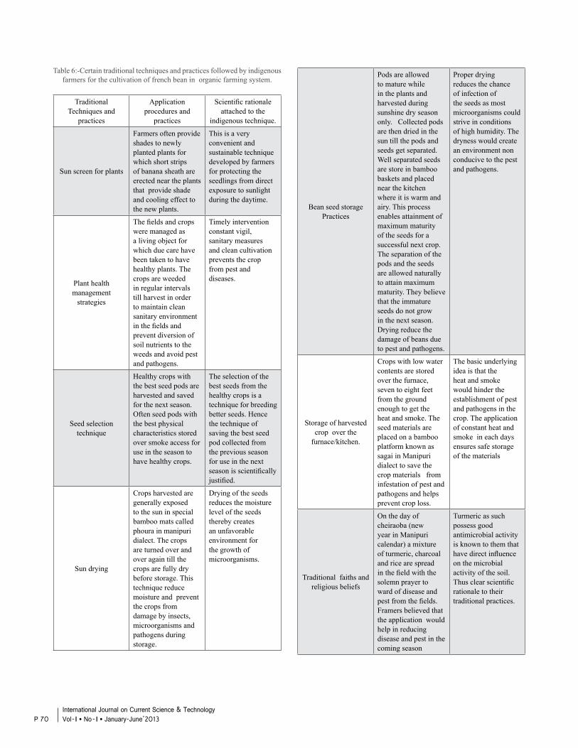
Table 6:-Certain traditional techniques and practices followed by indigenous farmers for the cultivation of french bean in organic farming system.
Traditional Techniques and
practices
Application procedures and
practices
Scientific rationale attached to the
indigenous technique.
Sun screen for plants
Farmers often provide shades to newly planted plants for which short strips of banana sheath are erected near the plants that provide shade and cooling effect to the new plants.
This is a very convenient and sustainable technique developed by farmers for protecting the seedlings from direct exposure to sunlight during the daytime.
Plant health management
strategies
The fields and crops were managed as a living object for which due care have been taken to have healthy plants. The crops are weeded in regular intervals till harvest in order to maintain clean sanitary environment in the fields and prevent diversion of soil nutrients to the weeds and avoid pest and pathogens.
Timely intervention constant vigil, sanitary measures and clean cultivation prevents the crop from pest and diseases.
Seed selection technique
Healthy crops with the best seed pods are harvested and saved for the next season. Often seed pods with the best physical characteristics stored over smoke access for use in the season to have healthy crops.
The selection of the best seeds from the healthy crops is a technique for breeding better seeds. Hence the technique of saving the best seed pod collected from the previous season for use in the next season is scientifically justified.
Sun drying
Crops harvested are generally exposed to the sun in special bamboo mats called phoura in manipuri dialect. The crops are turned over and over again till the crops are fully dry before storage. This technique reduce moisture and prevent the crops from damage by insects, microorganisms and pathogens during storage.
Drying of the seeds reduces the moisture level of the seeds thereby creates an unfavorable environment for the growth of microorganisms.
Bean seed storage Practices
Pods are allowed to mature while in the plants and harvested during sunshine dry season only. Collected pods are then dried in the sun till the pods and seeds get separated. Well separated seeds are store in bamboo baskets and placed near the kitchen where it is warm and airy. This process enables attainment of maximum maturity of the seeds for a successful next crop. The separation of the pods and the seeds are allowed naturally to attain maximum maturity. They believe that the immature seeds do not grow in the next season. Drying reduce the damage of beans due to pest and pathogens.
Proper drying reduces the chance of infection of the seeds as most microorganisms could strive in conditions of high humidity. The dryness would create an environment non conducive to the pest and pathogens.
Storage of harvested crop over the
furnace/kitchen.
Crops with low water contents are stored over the furnace, seven to eight feet from the ground enough to get the heat and smoke. The seed materials are placed on a bamboo platform known as sagai in Manipuri dialect to save the crop materials from infestation of pest and pathogens and helps prevent crop loss.
The basic underlying idea is that the heat and smoke would hinder the establishment of pest and pathogens in the crop. The application of constant heat and smoke in each days ensures safe storage of the materials
Traditional faiths and religious beliefs
On the day of cheiraoba (new year in Manipuri calendar) a mixture of turmeric, charcoal and rice are spread in the field with the solemn prayer to ward of disease and pest from the fields. Framers believed that the application would help in reducing disease and pest in the coming season
Turmeric as such possess good antimicrobial activity is known to them that have direct influence on the microbial activity of the soil. Thus clear scientific rationale to their traditional practices.
P 70International Journal on Current Science & Technology Vol - I l No- I l January-June’2013
REFERENCES
[1] Abiola Abioye,Yetunde Zaid,Halima S. Egberongbe, 2011, Documenting and Disseminating Agricultural Indigenous Knowledge For Sustainable Food Security: The Efforts of Agricultural Research Libraries in Nigeria, http://conference.ifla.org/ifla77
[2] Balasubramanian, A.V.,2006, Is there an Indian Way of Doing Science? In: Traditional Knowledge system of India and Sri Lanka, Balasubramanian and Nirmala Devi (eds.) pp. 183-192.
[3] Chhetry G.K.N. and Belbahri, Lassaad 2009, Indigenous pest and disease management practices in traditional farming systems in North east India: A review, Journal of plant breeding and crop science 1(3)28-38
[4] ICAR,Inventory of Indigenous Technical Knowledge in Agriculture, Document 1 (2002), Document 2 (2003), Supplement 1 to Document 2 (2003), Supplement 2 to Document 2 (2004), Document 3 (2004), Document 4 (2004), Document 5 9 2004). Indian Council of Agricultural Research, New Delhi.
[5] IIRR,1996, Recording and Using Indigenous Knowledge: A manual. International Institute of Rural Reconstruction, Silang, Cavite, Philippines
[6] Jeeva S.R.D.N., Laloo R.C. and Mishra, B.P.2006, Traditional agricultural practices in Meghalaya, North East India ,Indian Journal of Traditional Knowledge, 5(1)7-18
[7] Mane, P.M. and Sutaria, 1993, Study and documentation of Indigeneous knowledge/ traditional agricultural practices of the tribal farmers. Paper presented at national seminar on Indigenous Technologies for sustainable Agriculture.New delhi,March 23-25
[8] Nene. Y.L.,2006, Utilizing traditional knowledge systems of India and Srilanka. In: Traditional Knowledge system of India and Sri Lanka, Balasubramanian and Nirmala Devi (eds.) pp 32-38
[9] Pulmate, L and Babu, A.R. 1993, A seasoned exposition of the traditional farm practices under use by the farmers of Shifting and settled cultivation system in Manipur. Paper presented at the national seminar on indigenous technologies for sustainable agriculture, New Delhi, March 23-25.
[10] Ranganathan T.T. and Kumar S.A.,2006, Documentation and validation of traditional Agricultural practices.In: Traditional Knowledge system of India and Sri Lanka, Balasubramanian and Nirmala Devi (eds.) 40-61
[11] Sridevi R and Subhashini S. 2006, Traditional agricultural practices for crop testing -Testing and Validation. In: Traditional Knowledge system of India and Sri Lanka, Balasubramanian and Nirmala Devi (eds.) pp 62-67.
[12] Thurston, H.D.,1998, Traditional practices for plant disease management in traditional farming systems, http://www.tropag-fieldtrip.cornell.edu/tradag/default.html.
P 71International Journal on Current Science & Technology
Vol - I l No- I l January-June’2013

P 72International Journal on Current Science & Technology Vol - I l No- I l January-June’2013
INDUCED BREEDING OF EEL-LOACHPANGIO PANGIA, (HAMILTON 1822)
KH. GEETAKUMARI1, CH. BASUDHA2 & N. PRAKASH3
ICAR, Research Complex for NEH Region Manipur Centre, Lamphelpat Imphal-795004, Manipur, India.
E-mail : [email protected], [email protected]
ABSTRACT
The eel-loach Pangio pangia is a fish associated with the culture of Meitei community in Manipur. The preparation of the fish is fed to the newly married couple on the wedding night. The belief is that it makes the couple inseparable in life. The eel-loach are bottom feeders, omnivorous in nature, they eat worms and insect larvae. They inhabit in the fine bottom mud of its native creeks and lakes. In aquaria they are fed with small live, frozen foods, and pelleted feeds. They are shade lovers, peaceful and shy schooling fish. They usually hide themselves in PVC pipes or any hiding places like rocks, stones, etc. So, a soft sandy substrate is provided with lots of shady hiding places. Both males and females of Pangio pangia mature simultaneously. Mature females are probably noticeably plumber when loaded with eggs as seen with other Pangio species. They also prefer water quality having pH 7.5±0.2; dissolved oxygen, 6.0±2.0 ppm. Induced spawning of eel-loach Pangio pangia was successfully carried out using Wova-FH. The study reveals that the hormone inductions at the rate of 0.7ml/kg body weight of the breeders yields a potential fry stock. Hatching occurred within 3 hours after fertilization at water temperature 25-28 °C. The percentage of hatching rate varied from 85-90%. The yolk sac was absorbed on the second day of hatching. The outcome of this study can be effectively used for the captive breeding and conservation of the eel-loach, Pangio pangia.
Keywords : Induced breeding, Wova-FH, eel-loach, Pangio pangia
I. NTRODUCTION
Science is a socio-cultural activity that is highly disciplined The eel-loach Pangio pangia (Hamilton 1822) is a fish associated with the culture of Meitei community in Manipur. The preparation of the fish is fed to the newly married couple on the wedding night. The belief is that it makes the couple inseparable in life (Vishwanath, 2000). These loaches are also commonly collected and exported as aquarium fishes (Kottelat and Lim, 1993). Recently Pangio pangia has
undergone a drastic decline and is presently found missing. Perhaps it is due to loss of habitat, indiscriminate fishing, introduction of exotic species, water pollution, etc. therefore proper management initiatives of this species should be taken to conserve this fish. The knowledge on the proper breeding technique is one of them. Scanning of literature indicates that no thorough research have been done on the induced breeding of Pangio pangia.
Fish breeding is a convenient tool of environment and aquatic biology, education and self employment. It is a challenge that aquarist may find attractive. The primary concern of fish breeding is to produce the maximum number of the highest quality seeds and fingerlings from the available brood stock.Due to non-availability of seeds in natural waters and difficulty in artificial breeding of this fish, not much could be achieved towards commercialization of the species or conservation. Keeping this in view, it is now most important to conserve the species in a sustainable manner. The objective of this study was to breed Pangio pangia successfully under controlled conditions using Wova-FH and discuss its implications on the conservation of wild populations.
II. MATERIALS AND METHODS
Brood stock developmentPangio pangia fries were collected from Khumbong, Manipur during October, 2011. The fish fries were transported in oxygenated bags and stocked in FRP tanks of 3-ton water capacity with water recirculation system at ICAR, Campus. The fishes were fed with live feeds (daphnia, Cyclops) formulated diet.
Breeding experimentThe eel-loach earmarked for this study has been segregated from the common lot of fishes maintained at aquaria of ICAR-Research Centre, Imphal during May 2012. The male fish weighing 2.5g and female being 1.7g have been selected for the study. The males and female have been maintained separately and fed with live feed (Daphnia, Cyclops) and prepared feed containing protein density 50% for 10 days.Breeding is done in the evening 4 pm in 2:1 ratio, two males
P 73International Journal on Current Science & Technology
Vol - I l No- I l January-June’2013
and one female. A utility tray of (360×310×130) mm with a water depth of 8cm. Water quality of the spawning tray was analyzed by using water testing kits. The breeding trays were maintained with the following parameters-temperature, 25±3.0°C; pH, 7.5±0.2; dissolved oxygen, 6.0±2.0 ppm. A mild current is operated using an aerator.
The intramuscular injection of Wova-FH is given on the dorsal muscles above the lateral line near the dorsal fin. Three sets of brood stocks were selected at the ratio of 1:2 (female: male). Three different doses of Wova-FH i.e. 0.5ml, 0.7ml and 0.9ml/kg body weight were given to each set. After the injection, the breeding sets were released in the three utility trays.
Spawning occur after 21hrs of injection. After spawning, effective fecundity of each female was determined by randomly taking representative samples of eggs in a 10 ml graduated measuring cylinder from the total eggs in 1ml was counted and multiplied with total volume of egg released. The fertilization rate of egg was determined by randomly taking a sample of approx. 50 eggs.
EGGFertilized eggs were slight yellowish in colour, spherical, translucent and demersal measuring to 0.6-0.7 mm in diameter. Unfertilized eggs were paler and opaque. Within 1½ hours twitching movement of the embryo was observed. Hatching was preceded by movement of the larvae inside the egg shell. Fertilized eggs were hatched out after 3 hours of fertilization. The hatchlings were yellowish in colour.The newly hatched larvae measure 0.7- 1.5 mm long. The young ones did not take exogenous food for about 48 hrs at 25°C.
Larval RearingThe young ones are free swimming and very active in their environment. Very fast swimming movement was noticed in them. The yolk sac is fully absorbed at 60 hours. Once the yolk of the young ones is absorbed, they are fed with boiled egg.
Determining SexIt is difficult to determine the sex of the fish when they are young. In general the females are slightly larger than males of the same age. During the breeding season the females develop a swollen abdomen with a yellow tinge. While the males will ooze milt when gentle pressure is applied to the abdomen.
III. RESULTS
Brooders of Pangio pangia are found to be matured in the month of may in both the years 2011 and 2012. A varied degree of response of different doses of Wova-FH was
observed. Spawning response varied from 19-21 hours. Mating was preceded by elaborate courtship. It was observed that the male rubbed its body with the female and released its milt and the eggs were fertilized externally. Parental care was not seen in Pangio pangia. The highest rate of fertilization was obtained in the pair that was given a dose of 0.7ml/kg body weight.
IV. DISCUSSION
Induced breeding of Pangio pangia can be performed successfully in utility tray of (360l×310w×130h) mm. The temperature, dissolved oxygen and pH of the breeding tray are maintained throughout the experiment. A good chasing behavior was observed among the brooders. The number of eggs released and fertilized was comparatively examined. There is little information on induced breeding of Pangio pangia. This was our first attempt to breed this fish under control conditions.
From the results, it is evident that highest spawning of P. pangia occurred at close 0.7ml/kg. A lower dose of 0.5ml/kg was given and spawning was moderately low. Again a higher dose of 0.9ml/kg was given and a very low spawning was seen. The doses of hormone affected the percentage of fertilization and hatching rate. In our experiment, differences in the response of spawning were noticed in different sets.Similar observation was reported by Habibi et al. (1989) in Carassius auratus. Longer latency period was also reported by Pandey et al., (2002) in low dose of synthetic hormone Ovatide. The latency period of Ovaprim in air-breathing fishes is 18 hours for Channa puntatus and Heteropneustes fossilis (Haniffa et al, 2000). Pandey et al., (2002) reported varied inter-spawning period between 8 and 15 hour in Heteropneustes fossilis infected with the doses of 0.3-1.0ml/kg of synthetic hormone ovatide. According to Billiard et al. (1984) and Peter et al., (1986), differences in dose requirement may be attributed to varied level of dopamine activity in different species of fish.
In the present study, the incubation period lasted for 3hrs at a water temperature of 27°C. Kohli and Vidyagarthi (1990) reported the incubation period of 16-18h in Heteropneustes fossilis at a temperature of 26°C. Ramanathan et al. (1985) reported the incubation period in Mystus puntatus (Jerdon) to be varied from 18-24h at a temperature of 28.6 ± 1.8°C. Adebayo et al (2007) noted that hatching started at 22.0 ± 1.0 at the temperature of 25.50°C in African catfish. Zaki and Abdula (1983) and Herath (1988) reported shorter incubation periods at higher temperature. The development and incubation periods of embryo in most fishes are fully temperature dependent and varied from species to species (De Graaf and Janssen, 1996). Das et al. (2007) observed that the percentage of fertilization of eggs varied from 40-90 and the
P 74International Journal on Current Science & Technology Vol - I l No- I l January-June’2013
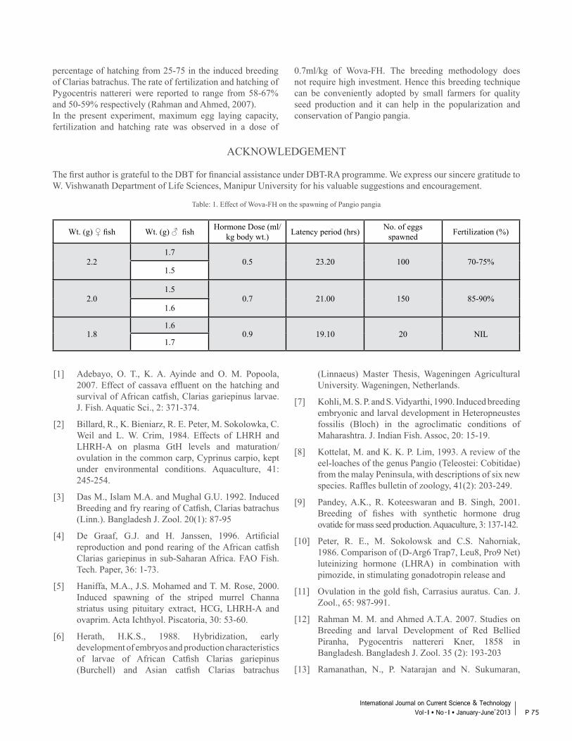
percentage of hatching from 25-75 in the induced breeding of Clarias batrachus. The rate of fertilization and hatching of Pygocentris nattereri were reported to range from 58-67% and 50-59% respectively (Rahman and Ahmed, 2007).In the present experiment, maximum egg laying capacity, fertilization and hatching rate was observed in a dose of
[1] Adebayo, O. T., K. A. Ayinde and O. M. Popoola, 2007. Effect of cassava effluent on the hatching and survival of African catfish, Clarias gariepinus larvae. J. Fish. Aquatic Sci., 2: 371-374.
[2] Billard, R., K. Bieniarz, R. E. Peter, M. Sokolowka, C. Weil and L. W. Crim, 1984. Effects of LHRH and LHRH-A on plasma GtH levels and maturation/ ovulation in the common carp, Cyprinus carpio, kept under environmental conditions. Aquaculture, 41: 245-254.
[3] Das M., Islam M.A. and Mughal G.U. 1992. Induced Breeding and fry rearing of Catfish, Clarias batrachus (Linn.). Bangladesh J. Zool. 20(1): 87-95
[4] De Graaf, G.J. and H. Janssen, 1996. Artificial reproduction and pond rearing of the African catfish Clarias gariepinus in sub-Saharan Africa. FAO Fish. Tech. Paper, 36: 1-73.
[5] Haniffa, M.A., J.S. Mohamed and T. M. Rose, 2000. Induced spawning of the striped murrel Channa striatus using pituitary extract, HCG, LHRH-A and ovaprim. Acta Ichthyol. Piscatoria, 30: 53-60.
[6] Herath, H.K.S., 1988. Hybridization, early development of embryos and production characteristics of larvae of African Catfish Clarias gariepinus (Burchell) and Asian catfish Clarias batrachus
0.7ml/kg of Wova-FH. The breeding methodology does not require high investment. Hence this breeding technique can be conveniently adopted by small farmers for quality seed production and it can help in the popularization and conservation of Pangio pangia.
ACKNOWLEDGEMENT
The first author is grateful to the DBT for financial assistance under DBT-RA programme. We express our sincere gratitude to W. Vishwanath Department of Life Sciences, Manipur University for his valuable suggestions and encouragement.
Table: 1. Effect of Wova-FH on the spawning of Pangio pangia
Wt. (g) fish Wt. (g) fish Hormone Dose (ml/kg body wt.) Latency period (hrs) No. of eggs
spawned Fertilization (%)
2.21.7
0.5 23.20 100 70-75%1.5
2.01.5
0.7 21.00 150 85-90%1.6
1.81.6
0.9 19.10 20 NIL1.7
(Linnaeus) Master Thesis, Wageningen Agricultural University. Wageningen, Netherlands.
[7] Kohli, M. S. P. and S. Vidyarthi, 1990. Induced breeding embryonic and larval development in Heteropneustes fossilis (Bloch) in the agroclimatic conditions of Maharashtra. J. Indian Fish. Assoc, 20: 15-19.
[8] Kottelat, M. and K. K. P. Lim, 1993. A review of the eel-loaches of the genus Pangio (Teleostei: Cobitidae) from the malay Peninsula, with descriptions of six new species. Raffles bulletin of zoology, 41(2): 203-249.
[9] Pandey, A.K., R. Koteeswaran and B. Singh, 2001. Breeding of fishes with synthetic hormone drug ovatide for mass seed production. Aquaculture, 3: 137-142.
[10] Peter, R. E., M. Sokolowsk and C.S. Nahorniak, 1986. Comparison of (D-Arg6 Trap7, Leu8, Pro9 Net) luteinizing hormone (LHRA) in combination with pimozide, in stimulating gonadotropin release and
[11] Ovulation in the gold fish, Carrasius auratus. Can. J. Zool., 65: 987-991.
[12] Rahman M. M. and Ahmed A.T.A. 2007. Studies on Breeding and larval Development of Red Bellied Piranha, Pygocentris nattereri Kner, 1858 in Bangladesh. Bangladesh J. Zool. 35 (2): 193-203
[13] Ramanathan, N., P. Natarajan and N. Sukumaran,
P 75International Journal on Current Science & Technology
Vol - I l No- I l January-June’2013

1985. Studies on the induced spawning and larval rearing of a fresh water catfish Mystus punctatus (Jerdon). Proc. Anim. Sci., 94: 389-398.
[14] Vishwanath, W. 2000. Fish Fauna of Manipur. Manipur Association for Science & Society, Imphal. ISBN 81-900689-5-4. 143 pp.
P 76International Journal on Current Science & Technology Vol - I l No- I l January-June’2013
[15] Zaki, M.I. and A. Abdula, 1983. The reproduction and development of Clarias gariepinus (Claridae) from Lake Manzala (Egypt). J. Ichthyol., 23: 48-58.
FUNGAL AIRSPORA OVER ONIONFIELD IN MANIPUR VALLEY
A. Premila
Department of Botany, Standard College, Imphal - 795001E-mail:[email protected]
ABSTRACT
Fungal airspora over onion field was monitored during two consecutive cropping seasons (Dec. 2009 - Apr. 2010 and Dec. 2010 - Apr. 2011) using Rotorod air sampler. Altogether 28 fungal types were isolated apart from other types (unidentified spores, hyphal fragments, pollengrains, insect scales etc.). Alternaria, Aspergilli - Penicilli, Botrytis, Cercospora, Curvularia, Cladosporium, Chaetominum, Helminthosporium, Nigrospora, etc. were dominant. Monthwise variation of fungal spores were observed. Concentration of fungal spores was highest in January in both the cropping seasons. The data were correlated with meteorological parameters.
Key words : airspora, meteorological parameters, onion, monthwise variation.
I. NTRODUCTION
Onion (Allium cepa) is the most widely cultivated species of the genus Allium. In Manipur, it is grown both in the valley and hilly regions. A variety of diseases and disorders affect onions. Most of the diseases are caused by fungi or bacteria. Among the fungal diseases of onion, neck rot caused by Botrytis allii, Leaf blight (Botrytis squamosa), downey mildew (Peronospora destructor), smut (Urocystis magica), white rot (Scelrotium cepivorum) and basal rot (Fusarium oxysporum) are considered most important. Contribution of fungal airspora to the occurrence and disease development on onion crop was reported by various workers (Devi, et. al. 2010; Lohare and Kareppa, 2009 and Maude and Prestly, 1977). Sen and Asan (2001) reported airborne fungi in vegetable growing areas of Edrine, Turkey. Devi (2010) analysed the fungal airspora of a cabbage field in Imphal. Devi and Chanu (2012) discussed the airspora and epidemiology of early blight of tomato in Manipur. So far, no detail study have been made on the airspora over onion field in Manipur. As such, the present investigation was undertaken to detect the major constituents of the fungal airspora over onion field and the effect of meteorological parameters on the occurrence of airborne fungi.
II. MATERIALS AND METHODS
Monitoring of fungal airspora over onion field was carried out using Tilak’s rotorod air sampler at Phayeng, Imphal West district, Manipur during two consecutive cropping seasons (Dec. 2009 - Apr. 2010 and Dec. 2010 Apr. 2011). In both the cropping seasons, air sampling was started on 1st Dec. (7 days prior to plantation of onion in the field) and continued upto the end of April (15 days after harvesting of the crop). The sampler was operated at 1 m above ground level at the centre of the onion field for 30 minutes at 10 day intervals. Identification of the fungal spores was done with the help of published literatures (Ellis, 1971; Barnett and Hunter, 1972 and Tilak, 1989) and by comparing with reference slides. The number of spores were multiplied by the conversion factor (5) of the sampler and expressed as per cubic metre of air. Scanning of the prepared slides was done regularly throughout the investigation period. Meteorological data for the investigation period were obtained from ICAR Research complex, Lamphelpat, Imphal.
III. RESULTS AND DISCUSSION
Analysis of the spores trapped revealed 27 fungal types. Hyphal fragments, pollen grains, insect scales, epidermal hairs, unidentified spores were grouped as “other types”. Table 1 revealed the percentage contribution of different spore types to the total airspora during the two consecutive cropping seasons. In the first cropping season (Dec. 2009 - Apr. 2010), fungal spores contributed 97.28% and other types contributed 2.72% of the total spore count. Cladosporium ranked highest concentration (18.45%) to the total airspora over onion field. Other dominant fungal types were Botrytis (9.03%), Alternaria (8.55%), Peronospora (7.31%), Fusarium (6.78%), Aspergilli-Penicilli (6.4%), Cercospora (5.38%), Helminthosporium (5.33%), round spores (Rhizopus-Mucor type) (3.43%), Nigrospora (3.02%), ascospores (2.55%) etc.
In the second cropping season (Dec. 2010 - Apr. 2011), fungal spores contributed 97.03% and other types contributed 2.97 % to the total airspora. Contribution of dominant spores types in descending order were Cladosporium (17.95%), Botrytis
P 77International Journal on Current Science & Technology
Vol - I l No- I l January-June’2013
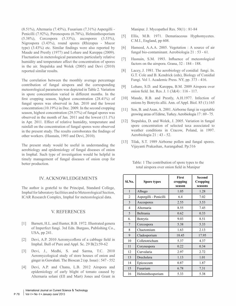
(8.51%), Alternaria (7.45%), Fusarium (7.31%) Aspergilli - Penicilli (7.92%), Peronospora (6.78%), Helminthosporium (5.38%), Cercospora (5.33%), ascospores (3.53%), Nigrospora (3.43%), round spores (Rhizopus - Mucor type) (3.43%) etc. Similar findings were also reported by Maude and Prestly (1977) and Lohare and Kareppa (2009). Fluctuation in meterological parameters particularly relative humidity and temperature affect the concentration of spores in the air. Stepalska and Wolek (2005) and Devi (2010) reported similar results.
The correlation between the monthly average percentage contribution of fungal airspora and the corresponding meteorological parameters was depicted in Table 2. Variation in spore concentration varied in different months. In the first cropping season, highest concentration (28.41%) of fungal spores was observed in Jan. 2010 and the lowest concentration (10.19%) in Dec. 2009. In the second cropping season, highest concentration (29.57%) of fungal spores was observed in the month of Jan. 2011 and the lowest (11.1%) in Apr. 2011. Effect of relative humidity, temperature and rainfall on the concentration of fungal spores were observed in the present study. The results corroborates the findings of other workers. (Hasnain, 1993 and Devi, 2010).
The present study would be useful in understanding the aerobiology and epidemiology of fungal diseases of onion in Imphal. Such type of investigation would be helpful in timely management of fungal diseases of onion crop for better production.
IV. ACKNOWLEDGEMENTS
The author is grateful to the Principal, Standard College, Imphal for laboratory facilities and to Meteorological Section, ICAR Research Complex, Imphal for meteorological data.
V. REFERENCES
[1] Barnett, H.L. and Hunter, B.B. 1972. Illustrated genera of Imperfect fungi. 3rd Edn. Burgass, Publishing Co., USA, pp 241.
[2] Devi, A.P. 2010 Aeromycoflora of a cabbage field in Imphal. Bull of Pure and Appl. Sc. 29 B(2):59-62
[3] Devi, J., Medhi, S. and Sarma, T.C. 2010 Aeromycological study of store houses of onion and ginger in Guwahati. The Bioscan 2 (sp. Issue) : 547 - 552
[4] Devi, A.P. and Chanu, L.B. 2012 Airspora and epidemiology of early blight of tomato caused by Alternaria solani (Ell and Mart) Jones and Grant in
Manipur. J. Mycopathol Res. 50(1) : 81-84
[5] Ellis, M.B. 1971. Dematiaceous Hyphomycetes. C.M.I., England, pp 608.
[6] Hameed, A.A.A. 2005. Vegetation : A source of air fungal bio-contaminant. Aerobiologia 21 : 53 - 61.
[7] Hasnain, S.M. 1993. Influence of meteorological factors on the airspora. Grana, 32 : 184 - 188.
[8] Lacey, J. 1981. The aerobiology of conidial fungi. In. G.T. Cole and B. Kendrick (eds), Biology of Conidial Fungi. Vol 1. Academic Press. NY, pp. 373 - 416.
[9] Lohare, S.D. and Kareppa, B.M. 2009 Airspora over onion field. Int. Res. J. 1 (3&4) : 116 - 117.
[10] Maude, R.B. and Prestly, A.H.1977. Infection of onions by Botrytis allii. Ann. of Appl. Biol. 85 (1):165
[11] Sen, B. and Asan, A. 2001. Airborne fungi in vegetable growing areas of Edirne, Turkey. Aerobiologia 17 : 69 - 75.
[12] Stepalska, D. and Wolek, J. 2005. Variation in fungal spore concentration of selected taxa associated to weather conditions in Cracow, Poland, in 1997. Aerobiologia 21 : 43 - 52.
[13] Tilak, S.T. 1989 Airborne pollen and fungal spores. Vijayanti Prakashan, Aurangabad. Pp:316
Table: 1 The contribution of spore types to thetotal airspora over onion field in Manipur
Sl.No. Spore typesFirst
cropping season
Second Cropping seasons
1 Albugo 1.05 1.282 Aspergilli - Penicilli 6.4 7.023 Ascospores 2.55 3.534 Alternaria 8.55 7.455 Beltrania 0.62 0.336. Botrytis 9.03 8.517 Cercospora 5.38 5.338 Chaetomium 1.63 2.139 Cladosporium 18.45 17.95
10 Colletotrichum 5.37 4.3711 Corynespora 0.22 0.3412 Curvularia 2.97 2.7213 Drechslera 1.13 1.0114 Epicoccum 0.87 1.8715 Fusarium 6.78 7.3116 Helminthosporium 5.33 5.38
P 78International Journal on Current Science & Technology Vol - I l No- I l January-June’2013
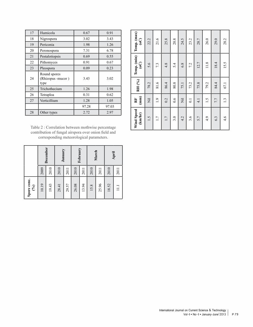
17 Humicola 0.67 0.9118 Nigrospora 3.02 3.4319 Periconia 1.98 1.2620 Peronospora 7.31 6.7821 Pestalotiopsis 0.69 0.5522 Pithomyces 0.91 0.6723 Pleospora 0.09 0.23
24Round spores (Rhizopus -mucor )type
3.43 3.02
25 Trichothecium 1.26 1.9826 Tetraploa 0.31 0.6227 Verticillium 1.28 1.05
97.28 97.0328 Other types 2.72 2.97
Table 2 : Correlation between mothwise percentage contribution of fungal airspora over onion field and
corresponding meteorological parameters.
Dec
embe
r
Janu
ary
Febr
uary
Mar
ch
Apr
il
2009
2010
2010
2011
2010
2011
2010
2011
2010
2011
Spor
e co
nc.
(%)
10.1
9
19.4
3
28.4
1
29.5
7
26.0
8
13.9
4
15.8
25.9
6
18.5
2
11.1
Tem
p. (m
ax)
(oC
)
22.2
21.6
25.8
20.8
24.5
23.2
28.7
26.0
29.0
28.2
Tem
p. (m
in)
(oC
)
5.6
7.3
4.8
5.4
6.8
7.2
12.7
11.8
18.4
15.5
RH
(%)
78.2
81.6
86.4
80.8
75.1
73.2
75.8
79.2
84.4
67.1
RF
(mm
)
Nil
1.9
0.2
0.6
Nil
0.1
4.1
1.5
7.7
1.3
Win
d Sp
eed
(km
/hr)
1.5
1.7
1.7
3.0
4.2
3.6
5.7
4.9
6.3
4.6
P 79International Journal on Current Science & Technology
Vol - I l No- I l January-June’2013

P 80International Journal on Current Science & Technology Vol - I l No- I l January-June’2013
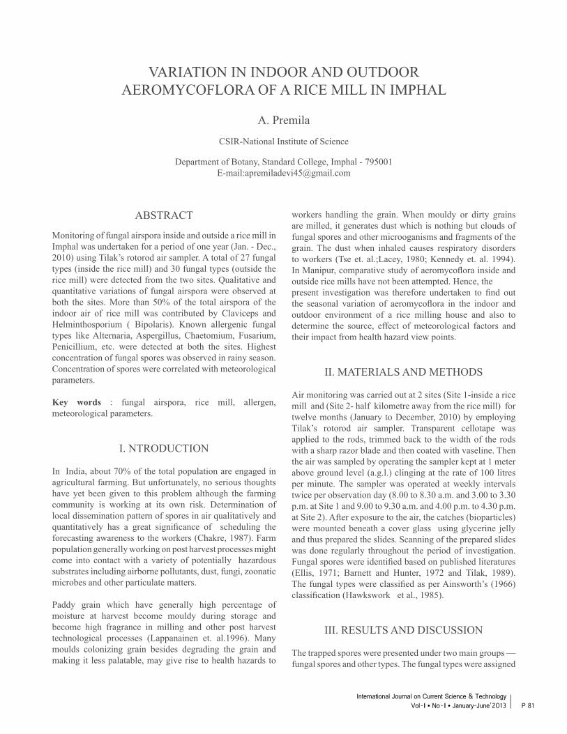
VARIATION IN INDOOR AND OUTDOOR AEROMYCOFLORA OF A RICE MILL IN IMPHAL
A. Premila
CSIR-National Institute of Science
Department of Botany, Standard College, Imphal - 795001E-mail:[email protected]
ABSTRACT
Monitoring of fungal airspora inside and outside a rice mill in Imphal was undertaken for a period of one year (Jan. - Dec., 2010) using Tilak’s rotorod air sampler. A total of 27 fungal types (inside the rice mill) and 30 fungal types (outside the rice mill) were detected from the two sites. Qualitative and quantitative variations of fungal airspora were observed at both the sites. More than 50% of the total airspora of the indoor air of rice mill was contributed by Claviceps and Helminthosporium ( Bipolaris). Known allergenic fungal types like Alternaria, Aspergillus, Chaetomium, Fusarium, Penicillium, etc. were detected at both the sites. Highest concentration of fungal spores was observed in rainy season. Concentration of spores were correlated with meteorological parameters.
Key words : fungal airspora, rice mill, allergen, meteorological parameters.
I. NTRODUCTION
In India, about 70% of the total population are engaged in agricultural farming. But unfortunately, no serious thoughts have yet been given to this problem although the farming community is working at its own risk. Determination of local dissemination pattern of spores in air qualitatively and quantitatively has a great significance of scheduling the forecasting awareness to the workers (Chakre, 1987). Farm population generally working on post harvest processes might come into contact with a variety of potentially hazardous substrates including airborne pollutants, dust, fungi, zoonatic microbes and other particulate matters.
Paddy grain which have generally high percentage of moisture at harvest become mouldy during storage and become high fragrance in milling and other post harvest technological processes (Lappanainen et. al.1996). Many moulds colonizing grain besides degrading the grain and making it less palatable, may give rise to health hazards to
workers handling the grain. When mouldy or dirty grains are milled, it generates dust which is nothing but clouds of fungal spores and other microoganisms and fragments of the grain. The dust when inhaled causes respiratory disorders to workers (Tse et. al.;Lacey, 1980; Kennedy et. al. 1994). In Manipur, comparative study of aeromycoflora inside and outside rice mills have not been attempted. Hence, the present investigation was therefore undertaken to find out the seasonal variation of aeromycoflora in the indoor and outdoor environment of a rice milling house and also to determine the source, effect of meteorological factors and their impact from health hazard view points.
II. MATERIALS AND METHODS
Air monitoring was carried out at 2 sites (Site 1-inside a rice mill and (Site 2- half kilometre away from the rice mill) for twelve months (January to December, 2010) by employing Tilak’s rotorod air sampler. Transparent cellotape was applied to the rods, trimmed back to the width of the rods with a sharp razor blade and then coated with vaseline. Then the air was sampled by operating the sampler kept at 1 meter above ground level (a.g.l.) clinging at the rate of 100 litres per minute. The sampler was operated at weekly intervals twice per observation day (8.00 to 8.30 a.m. and 3.00 to 3.30 p.m. at Site 1 and 9.00 to 9.30 a.m. and 4.00 p.m. to 4.30 p.m. at Site 2). After exposure to the air, the catches (bioparticles) were mounted beneath a cover glass using glycerine jelly and thus prepared the slides. Scanning of the prepared slides was done regularly throughout the period of investigation. Fungal spores were identified based on published literatures (Ellis, 1971; Barnett and Hunter, 1972 and Tilak, 1989). The fungal types were classified as per Ainsworth’s (1966) classification (Hawkswork et al., 1985).
III. RESULTS AND DISCUSSION
The trapped spores were presented under two main groups — fungal spores and other types. The fungal types were assigned
P 81International Journal on Current Science & Technology
Vol - I l No- I l January-June’2013
to five subdivisions as per Ainsworth’s (1966) classification (Hawkswork et al., 1985) (Table 1). Quantitative and qualitative variations in the incidence of the different components of airspora inside and outside the rice mill were observed in the present study.In Site 1, Deuteromycotina dominated the fungal airspora of both sites by scoring 57.32% of the total population which was followed by Ascomycotina (30.67%), other types (6.81), Basidiomycotina (4.83%), Zygomycotina (0.0.37%) and Mastigomycotina (Nil). Among the fungal types, Claviceps contributed highest concentration (27.02%), Helminthosporium ( Bipolaris) (25.51%) which was followed by Nigrospora (6.68%), Aspergilli-Penicilli (5.95%), Fusarium (5.6%), Pyricularia (4.38%), Curvularia (2.81%), fusiform ascospores (2.74%), basidiospores (2.65%), Alternaria (2.61%), Sclerotium (2.23%), uredospores (2.18%), etc.
In Site 2, Deuteromycotina dominated the fungal airspora by scoring 73.05% of the total population which was followed by Mastigomycotina (13.66%), other types (8.63%),Ascomycotina (3.2%), Zygomycotina (1.37%) and Basidiomycotina (0.09%). Among the fungal types, Cladosporium contributed highest concentration (21.49%) which was followed by Aspergilli-Penicilli (19.67%), Albugo (13.66%), Fusarium (9.23%), Curvularia (6.57%), Alternaria (5.49%), Pestalotiopsis (4.51%), Chaetomium (3.05%), Nigrospora (2.47%), round spores (Rhizopus - Mucor type) (1.37%), Sclerotoium (1.08%), etc. This was in agreement with the reports of earlier workers (Gimenez et. al. 1995 and Singh and singh, 2005).
The present finding clearly showed Claviceps and Helminthosporium ( Bipolaris) as predominant among the dominant types contributing more than 10% each to the total count. This might be due to the diffusive action of machines while milling the raw materials i.e. paddy grains physically contaminated with smut (Claviceps) and brown spot (Helminthosporium ). Perusal and analysis on the results from different working environments and sources like dust from bags, floors, walls, dust pasted on different parts of equipments and machines, etc. present in the working room showed a normal source of fungi within the rice mill. The present finding was in congruity with results reported earlier (Singh and Singh, 2005).
The incidence of certain spore types like Aspergilli-Penicilli, Cladosporium, Curvularia, Fusarium, Pestalotiopsis, etc. were drastically higher in Site 2 which might be due to the specific composition of local vegetation and ecological entities of the surrounding environment. Hasnain (1993) and Hameed (2005) reported similar results. Fig. 1 revealed the quantitative seasonwise variations of airspora at both the investigation sites. The highest
Fig: 1 - Seasonwise variations of total indoor fungalairspora inside and outside the rice mill during 2010..
concentration (40.56% in Site 1 and 42.83% in Site 2) of airspora was observed in rainy season which corresponds to temperature (max. 28.60C and min. 22.220C), relative humidity (89.5%), rainfall (7.4 mm) and wind speed (2.7 km/hr) and the lowest (19.5% in Site 1 and 16.28% in Site 2) in winter season which corresponds to temperature (max. 23.90C and min. 6.30C), relative humidity (81%), rainfall (0.7 mm) and wind speed (2.5 km/hr). It was evident from the above findings that there was a wide range of relative humidity and temperature in between the distribution of highest and lowest concentration of fungal airspora. Thus showed the close correlation between the concentration of airspora and the effects of favourable meteorological factors besides other artificial factors like availability of abundant substrates, shaking and agitation of milling machines, etc. The finding was in agreement with that of other workers (Hasnain, 1993; Singh and Singh, 2005 and Devi and Singh, 2007).
Allergenic biopollutants and biodeteriogenic fungal spores comprised major share in the airspora of indoor air of rice mill in Imphal area. In the present study, a large number of known allergenic fungal spore types like Aspergillus, Chaetomium, Cladosporium, Curvularia, Epicoccum, Fusarium, Helminthosporium, Mucor, Penicillium, Rhizopus, etc. which are known to be associated with respiratory and other allergy (Agarwal and Shivpuri, 1974) were freely present in the indoor air of rice mill. Working more duration continuously for long time might cause harmful effect to the workers.Similar trend of present study in far and depth might be beneficial in detection of outbreak of occupational hazards and similar health problems to the mill workers. Further, it is suggested that air monitoring of biopollutants and biodeterioagents be made in rice mills and similar working environments in Imphal and other parts of the state.
≡
0
5
10
15
20
25
30
35
40
45
Spor
e co
nc.(%
)
Winter (Dec - Feb.) Summer (March - May)
Rainy (June - Sept) Retreating monsoon(Oct. - Nov.)
Site 1 Site 2
P 82International Journal on Current Science & Technology Vol - I l No- I l January-June’2013
Table 1: Percentage contribution of different spore typesin the indoor and outdoor air of rice mill in Imphal during 2010.
Sl. No. Spore types Percentage contribution of sporesSite 1 (inside the rice mill)
Site 2 (outside the rice mill)
MASTIGOMYCOTINA1. Albugo - 13.66
ZYGOMYCOTINA1. Round spores
(Rhizopus- Mucor type)
0.37 1.37
ASCOMYCOTINA1. Chaetomium 0.90 3.052. Claviceps 27.02 –3. Fusiform ascospores 2.74 0.154. Pleospora 0.01 –
30.67 3.20BASIDIOMYCOTINA
1. Basidiospores 2.65 0.092. Uredospores 2.18 –
4.83 0.09DEUTEROMYCOTINA
1. Alternaria 2.61 5.492. Aspergilli– Penicilli 5.95 19.673. Beltrania 0.01 0.714. Bispora 0.01 0.355. Cercospora 0.34 0.206. Cladosporium 0.39 21.497. Colletotrichum – 0.108. Corynespora 0.01 0.109. Curvularia 2.81 6.5710. Diplodia – 0.0111. Drechslera 0.46 0.0812. Epicoccum 0.10 0.0113. Fusarium 5.60 9.2314. Helminthosporium
(= Bipolaris)25.51 –
15. Memnoniella 0.03 0.0116. Nigrospora 6.68 2.4717. Periconia 0.05 0.0218. Pestalotiopsis 0.01 4.5119 Pithomyces 0.01 0.3020 Pyricularia 4.38 –21 Sclerotium 2.23 1.0822 Spegazzinia 0.01 0.05
23 Stemphylium 0.03 –24. Tetraploa 0.05 0.0325 Torula 0.04 0.5426 Trichoconis – 0.0227 Trichothecium – 0.01
57.32 73.05OTHER TYPES 6.81 8.63GRAND TOTAL 100 100
IV. ACKNOWLEDGEMENTS
The author is grateful to the Principal, Standard College, Imphal for laboratory facilities and to Meteorological Section, ICAR Research Complex, Imphal for meteorological data.
V. REFERENCES
[1] Agarwal, M.K. and Shivpuri, D.N. 1974 Fungus spores: their role in respiratory allergy. Adv. in Pollen Spore Res., 1:78-128.
[2] Ainsworth, G.C. 1966 A general purpose classification for fungi. Bibl. Syst. Mycol., 1: 1-4.
[3] Barnett, H.L. and Hunter, B.B. 1972. Illustrated genera of Imperfect fungi. 3rd Edn. Burgass, Publishing Co., USA, pp 241.
[4] Chakre, O.J. 1987 Agricultural practices too pollute environment. Science Reporter, (7): 376.
[5] Devi, A.P. and Singh, N.I. 2007 Indoor aeromycology of certain workplace environments in Manipur and their management practices, in N.I. Singh (Ed.), Endemic bioresources of India, (Bishen Singh Mahendra Pal Singh,) 35-44.
[6] Gimenez, C., Fouad, K., Choudat, D., Laurillard, J., Bouscaillou, P. and Leib,E. 1995 Chronic and acute respiratory effects among grain mill workers. Int. Arch. Occup. Environ. Health, 67(5): 311-316.
[7] Ellis, M.B. 1971. Dematiaceous Hyphomycetes. C.M.I., England, pp 608.
[8] Hameed, A.A.A. 2005. Vegetation : A source of air fungal bio-contaminant. Aerobiologia 21 : 53 - 61.
[9] Hasnain, S.M. 1993. Influence of meteorological factors on the airspora. Grana, 32 : 184 - 188.
[10] Hawkswork, D.L., Sutton, B.C. and Ainsworth, G.C. 1985 Dictionary of the fungi. International Books and Periodicals Supply Service, New Delhi.
P 83International Journal on Current Science & Technology
Vol - I l No- I l January-June’2013
[11] Kennedy, S.M., Dimichward, H., Desjardins, A., Kassam, A., Vedal, S. and Chan Young, M. (1994) Respiratory health among retired grain elevator workers. Amer. J. Respir. Crit. Care Med., 150(1):59-65.
[12] Lacey, J. 1980 The microflora of grain dust. In: Occupational pulmonary disease: focus on grain dust and health. (Eds J.A. Doseman and D.A. Cotton) Academic Press, New York, pp 417-440.
[13] Lappalainen, S., Nikulin, M., Berg, S., Parikka, P., Hintikka, E.L. and Pasanen, A.L. 1996 Fusarium toxins and fungi associated with handling of grain on
eight Finnish farms. Atmos. Environ., 30(17):3059-3066.
[14] Singh, W.M. and Singh, N.I. 2005 Indoor aeromycoflora of rice mill Bishnupur, Manipur. Indian J. Aerobiol. 18 (1) : 24 - 31.
[15] Tse, K.S., Warren, P., Janusz, M., McCarthy, D.S. and Cherniak, R.M. 1973 Respiratory abnormalities in workers exposed to grain dust. Arch. Environ. Health, 27: 74-77.
[16] Tilak, S.T. 1989 Airborne pollen and fungal spores. Vijayanti Prakashan, Aurangabad. Pp:316
P 84International Journal on Current Science & Technology Vol - I l No- I l January-June’2013

BIOCHEMICAL NETWORKS: THE CHEMISTRY OF LIFE
Rhythm Upadhyaya
Department of Information TechnologyAssam University, Silchar,India
E-mail : rhythm [email protected]
Rhyme Upadhyaya
Department of Information TechnologyFuture Institute Of Engineering and Management
West Bengal University of Technology, Kolkata,IndiaE-mail : [email protected]
ABSTRACT
Biochemical networks are the central processing units of life. They can perform a variety of computational tasks analogous to electronic circuits. Their design principles, however, are markedly different: in a biochemical network, computations are performed by molecules that chemically and physically interact with each other. Biochemical networks can be viewed as interconnected processes forming an intricate network of functional and physical interactions between molecular species in the cell. The amount of information available on such pathways for different organisms is increasing very rapidly. This is offering the possibility of performing various analyses on the structure of the full network of pathways for one organism as well as across different organisms. Various forms of data models have been devised for the analysis of biochemical networks.
Index Terms : Biochemistry, Metabolic pathways, Gene regulatory, Signaling pathways.
I. NTRODUCTION
Biochemical Networks are molecular interaction network in biological processes. Analysis of Biochemical Networks, deals with abstractions, algorithms, and statistical models, for gathering information from a broad class of rapidly emerging datasets, referred to as biochemical networks. While domain experts see great value in such data and how it can be used for phenotype characterization, knockout experiments, drug design, and, in general, understanding the biochemical processes in the cell, there is increasing realization that the computational framework needed to answer the questions needs to be developed. The techniques for generating, validating, and analyzing network data are contributing directly to the broader systems view to biology. A key aim of postgenomic biomedical research is to systematically catalogue all molecules and their interactions within a living cell. There is a clear need to understand how these molecules and the interactions between them determine
the function of this enormously complex machinery, both in isolation and when surrounded by other cells. Rapid advances in network biology indicate that cellular networks are governed by universal laws and offer a new conceptual framework that could potentially revolutionize our view of biology and disease pathologies in the twenty-first century. Identifying the sources of variations and flow of information in biochemical networks is to understand how cells control and exploit biochemical fluctuations. we must identify the sources of stochasticity and quantify their effects. Cellular biochemical networks are highly interconnected: a perturbation in reaction rates or molecular concentrations may affect numerous cellular processes..
II.TYPES OF BIOCHEMICAL NETWORKS
Biochemical networks represent the biological reactions and interaction network in a cell. Each reaction is identified with its enzyme, which in turn is coded by certain gene(s). In [1]There are three types of biochemical networks- Metabolic Pathways, Gene Regulatory Pathways , Signaling Pathways.
[a] Metabolic Pathways:Metabolic Pathways are series of chemical reactions occurring within a cell. In each Metabolic Pathway a principal chemical is modified by a series of chemical reactions. Each metabolic pathway consists of a series of biochemical reactions that are connected by their intermediates: the products of one reaction are the substrates for subsequent reactions, and so on. Metabolic pathways are often considered to flow in one direction. Although all chemical reactions are technically reversible, conditions in the cell are often such that it is thermodynamically more favorable for flux to flow in one direction of a reaction. For example, one pathway may be responsible for the synthesis of a particular amino acid, but the breakdown of that amino acid may occur via a separate and distinct pathway. One example of an exception to this “rule” is the metabolism of glucose. Glycolysis results in the breakdown of glucose, but several reactions in the glycolysis pathway are reversible and
P 85International Journal on Current Science & Technology
Vol - I l No- I l January-June’2013
participate in the re-synthesis of glucose (gluconeogenesis). Some more examples of metabolic pathways include Phosphorylation, Kreb’s Cycle etc. Metabolic pathways are often regulated by feedback inhibition Some metabolic pathways flow in a ‘cycle’ wherein each component of the cycle is a substrate for the subsequent reaction in the cycle, such as in the Krebs Cycle.
[b] Gene Regulatory Pathways: In [5] A regulatory pathway is a coordinated series of reactions and molecular interactions regulating the expression and/or activity of enzymes and transporters. It consists of set of genes, proteins, small molecules, and their mutual regulatory interactions. Gene regulatory networks explicitly represent the causality of developmental processes. They explain exactly how genomic sequence encodes the regulation of expression of the sets of genes that progressively generate developmental patterns and execute the construction of multiple states of differentiation. Gene regulatory networks are inhomogeneous compositions of different kinds of subcircuits, each performing a specific kind of function. A genetic network consists of a set of genes that are related through a collection of regulatory proteins. Each gene may require an input and may produce an output. A gene’s output results in the production of either regulatory or constructive proteins. Regulatory proteins act as inputs for the other genes and affect their expression, while constructive proteins make up the physical structure of the organism.The modelling of gene regulatory networks relies on characterization of the behaviour of small subsystems, formation of hypotheses about how these subsystems interconnect, translation of these hypotheses into a mathematical model and experimentation to yield results that indicate necessary changes to the original hypotheses.
[c] Signaling Pathways:In [2] Finally, signal transduction is a term describing the transfer of information (called signals)from one cellular location (often the extracellular medium) to another (often the cell nucleus); a signal transduction pathway is coordinated series of reactions and interactions realizing a signal transduction. Cell-cell interactions through signal-transduction pathways are crucial in the coordination of embryonic development.Typically, signalling pathways are activated by the binding of a ligand to a transmembrane receptor, which in turn leads to the modificationof cytoplasmic transducers. Subsequently, these transducers activate transcription factors that ultimately alter gene expression.One of the most surprising findings about signaling processes is that only a few pathways are involved in and are responsible for most of cell development. Until recently, studies of the evolution of signalling pathways were carried out by searching for the individual components of these pathways in those organisms considered to represent
taxa that were phylogenetically informative for metazoan evolution. 4 types of intercellular signaling -Endocrine, Paracrine, Neuronal signaling, Contact-dependent signaling.signalling pathways are nonlinear, highly integrative biological modules with robust properties that ensure reproducible outcomes of developmental processes.At the same time, however, they are flexible enough to allow changes in the signaling response during development and evolution.
III. BIOCHEMICAL NETWORKDATABASES AND TOOLS
[a] Databases : In [1] They hold data on biochemical pathways and their components (e.g. enzymes, substrates,products) and on the correponding interactions and chemical reactions. They are encyclopedic references for pathway information; they can be queried for information retrieval, and can be analysed through computer programs.
Some existing databases focus on specific types of interactions e.g. BRENDA (enzymatic catalysis) , DIP (protein-protein interactions), Transfac (protein-DNA interactions , and RegulonDB (protein-DNA interactions) There are several databases on metabolic pathways, such as KEGG (genes, enzymes, metabolic reactions) , EMP (enzymes, pathways) and WIT (metabolic pathway reconstruction), EcoCyc (metabolic pathways, E.coli) and MetaCyc (metabolic pathways of other organisms), aMAZE , CSNDB, PathDB UM-BBD, SHARKdb, etc. The BIND database contains information on interactions that take part in signal transduction pathways. An analysis and comparison of these databases can be found in . In most databases the information is represented in a (simple) relational form. The quality of the underlying relational data model is important for the extraction of suitable information for analysing the networks.
[a.1] Metabolic Pathways Databases:In [9] Compendium of pathways describing metabolic and physical processes (Primary source for metabolic information initiated by Stanford Research Initiative) .ECOCYC- Entire genome and biochemical machinery of E. coli , METACYC- Pathways of more than 165 species, HUMANCYC- Human metabolic pathways and the human genome, BIOCYC- Collection of databases for several organism, KEGG-Comprehensive Links to several useful databases
[a.2] Gene Regulatory Databases:In [9] Organize experimental and/or in silico interactions .BIND -200,000 documented biomolecular interactions and complexes, MINT- Experimentally verified interactions,HPRD -Elegant and comprehensive presentation
P 86International Journal on Current Science & Technology Vol - I l No- I l January-June’2013
of the interactions, entities,and evidences, MPACT- Yeast interactions. A part of MIPS, DIP -Experimentally determined interactions.INTACT- Database and analysis system of binary and multiprotein interactions,PDZBASE-PDZ Domain containing proteins, GNPV- Based on specific experiments and literature, BIOGRID- Physical and genetic interactions,UNIHI- Comprehensive human protein interactions, OPHID -Combines PPI from BIND, HPRD, and MINT.
TiGER (Tissue-specific Gene Expression and Regulation) is a database for generating comprehensive information about human tissue-specific gene regulation, including bothexpression and regulatory data.
[a.3] Signaling Pathways Databases:In [9] Pathways pertaining to signal transduction. PANTHER- Compendium of pathways built using CellDesigner , REACTOME-Hierarchical layout. Extensive links to relevant databases
BIOMODELS - Domain experts curated pathways and associated mathematical models. STKE- Repository of canonical pathways.INGENUITY- Systems Commercial mammalian biological knowledgebase, PID -Compendium of several assembled signaling pathways, BIOPP -Repository of biological pathways built using CellDesigner.
[b] Pathway tools:Pathway tools are comprehensive software environment that supports construction of organism specific databases.Pathway building tools are required to populate, visualize, and store a pathway. Currently there ar various pathway building tools that provide the ability to extract information as well as to support multiple standard formats. Cytoscape, CellDesigner, and JDesigner are graphical environments for constructing pathways that can import/export SBML models for simulation.
[b.1] Metabolic Pathway Tools:RAHNUMA (Hypergraph based tool), ARCADIA (A visualization tool for metabolic pathways.),UTOPIA(model/view/controller pattern.)PW-COMP(A graph comparative tool),ELEMENTARY MODE ANALYSIS(characterizing cellular metabolism), KATSURA,PATHWAY HUNTER TOOL(shortest pathway analysis)
[b.2] Gene regulatory tools:GENEVIS-(provides a visual environment for exploring the dynamics of genetic regulatory networks),PAINT(promoter analysis and interaction network toolset),ZLAB,TRANSFAC(Transcriptional Gene regulation in eukaryotes),MicroRNAS(regulate gene expression in a sequence specific manner), ARIADNE.
[b.3] Signaling pathway tools:STATS(signal transducers and activators of transcription), Cell Surface Receptor.
Pathway Tools supports analysis of omics datasets (e.g., gene expression and metabolomics) by painting omics data onto a diagram of the full metabolic map of the organism, or onto a diagram of the full regulatory network. Pathway Tools also computes several variations of enrichment analysis. Pathway Tools performs metabolic network analyses including finding choke points (potential drug targets) in metabolic networks, dead-end metabolite analysis, and reachability analysis. Pathway Tools has its own genome browser, which has a microbial orientation. In addition, Pathway Tools can be coupled with other genome browsers to add support for pathways to an existing MOD, such as was done for SGD and DictyBase.
IV. ANALYSIS AND MODELLINGOF BIOCHEMICAL NETWORKS
In [1] Kinetic models detail the interaction between substrates and enzymes; they involve the solution of differential equations, for which several quantitative parameters have to be specified. Finally, metabolic control analysis is concerned with quantifying the control of flux among enzymes. [1]Metabolic flux analysis considers models that relate to the quantification of flux. It is based on the principle of mass conservation. It requires information on stoichiomtry; no data on enzyme kinetic is required. This includes metabolic balancing and isotopic balancing. Petri nets have been widely used for the formalisation and the simulation of biochemical processes.[1]Petri nets, an active research domain in computer science and mathematics, are a graph-oriented formalism allowing the modelling and analysis the concurrent behaviour of systems. Petri nets are special bipartite graphs with an associated semantics. The two types of nodes are place nodes and transition nodes In [12] Computer modelling and simulation are commonly used to analyse engineered systems.Biological systems differ in that they often cannot be accurately characterized, so simulations are far from exact. evolution results in recurring, dynamic organizational principles in biological systems, and that simulation can help to identify them and analyse their dynamic properties. By contrast, the components of biological systems are difficult to characterize. The kinetic behaviour of a protein specie may depend on its amount, conformation, cellular location, and the milieu of other molecules present in the cell at the same time. None of these variables can be defined exactly. Many are fundamentally only definable as members of Fuzzy Sets with intrinsically noisy distribution profiles. Moreover, experimental
P 87International Journal on Current Science & Technology
Vol - I l No- I l January-June’2013
measurement of molecular concentrations, protein states, interaction kinetics, etc. is inherently inexact. In-vitro measurements often do not reflect conditions inside a cell and can be orders of magnitude different from in -vivo values. In-vivo measurements, on the other hand, can currently only be carried out by proxy and provide very approximate values. For instance, the long half-life of Green Fluorescent Protein (as well as Luciferase and other reporters), means that in -vivo measurements represent the time-average (integral) of an activity, not its instantaneous value. Complex networks of biochemical reactions, such as intracellular protein signaling pathways and genetic networks, are often conceptualized in terms of ``modules,’’ semi-independent collections of components that perform a well-defined function and which may be incorporated in multiple pathways. However, due to sequestration of molecular messengers during interactions and other effects, collectively referred to as retroactivity, real biochemical systems do not exhibit perfect modularity. Biochemical signaling pathways can be insulated from impedance and competition effects, which inhibit modularity, through enzymatic ``futile cycles’’ which consume energy, typically in the form of ATP. In[13] We have developed BioNetS to be a reliable model for studying the stochastic dynamics of large biochemical networks. Important features of BioNetS are its ability to handle hybrid models that consist of both continuous and discrete random variables and its ability to model cell growth and division. We have verified the accuracy and efficiency of the numerical methods by considering several test systems. We have developed the software package Biochemical Network Stochastic Simulator (BioNetS) for efficiently and accurately simulating stochastic models of biochemical networks. BioNetS has a graphical user interface that allows models to be entered in a straightforward manner, and allows the user to specify the type of random variable (discrete or continuous) for each chemical species in the network. The discrete variables are simulated using an efficient implementation of the Gillespie algorithm. For the continuous random variables, BioNetS constructs and numerically solves the appropriate chemical Langevin equations. The software package has been developed to scale efficiently with network size, thereby allowing large systems to be studied. In [14],we introduce the use of ShReD as a round trip distance metric, which can be combined with a partition algorithm (adapted from Newman’s earlier work on community detection) to systematically identify biochemical reaction modules that feature cyclical interactions. The notion of grouping together network components based on “retroactivity” was first proposed by Saez-Rodriguez and coworkers, who hypothesized that a strictly downstream component should have little impact on the activity of an upstream component unless there is a feedback or retroactive relationship. It has been suggested that such feedback relationships contribute to robustness with respect to external perturbation, notably
in signal transduction networks The ShReD metric accounts for cyclical interactions that span multiple reaction steps, and thus significantly extends on the prior work on retroactivity, which focused on local interactions between neighboring components. Previously, (shortest) path lengths between network components have been used to identify reaction modules by clustering, but without consideration of directionality and retroactivity . In[14] The signaling network was reconstructed based on a published model of epidermal growth factor receptor (EGFR) signaling . The model was downloaded as an SBML file and cast into the form of a stoichiometric matrix based on the directional interactions between signaling molecules defined in the SBML file. The model consisted of 322 signaling molecules (metabolites and proteins) participating in 211 signaling reactions. In addition to the signaling reactions, the model includes 238 allosteric interactions between the signaling molecules and reactions. The reactions in this model were a priori assigned to groups based on their previously catalogued function . For example, the reactions that convert ERK1/2 and PKB/akt into their active forms were assigned to the MAPK cascade and PIP signaling, respectively. This initial grouping, which reflects historical knowledge of signaling modularity, provided a basis for comparison between biological knowledge-driven, canonical associations versus partition-driven, systematically obtained network modules.In[14] A stoichiometric network model of human hepatocyte metabolism was reconstructed from the KEGG reaction database and further augmented by the addition of xenobiotic transformation reactions, as well as regulatory interactions mediated by allosteric effectors. The model comprised 159 reactions, 146 metabolites, and 61 regulatory interactions. The xenobiotic transformation reactions were added to describe the metabolism of the anti-diabetic compound troglitazone (TGZ), including steps needed to supply conjugation substrates such as glutathione (GSH).
In[15] Understanding of the logic and dynamics of gene-regulatory and biochemical networks is a major challenge of systems biology. To facilitate this research topic, we have developed a modeling/simulating tool called CellDesigner. CellDesigner primarily has capabilities to visualize, model, and simulate gene-regulatory and biochemical networks. Two major characteristics embedded in CellDesigner boost its usability to create/import/export models: 1) solidly defined and comprehensive graphical representation (systems biology graphical notation) of network models and 2) systems biology markup language (SBML) as a model-describing basis, which function as intertool media to import/export SBML-based models. In addition, since its initial release in 2004, we have extended various capabilities of CellDesigner. For example, we integrated other systems biology workbench enabled simulation/analysis software packages. CellDesigner also supports simulation and
P 88International Journal on Current Science & Technology Vol - I l No- I l January-June’2013
parameter search, supported by integration with SBML ODE Solver, enabling users to simulate through our sophisticated graphical user interface. Users can also browse and modify existing models by referring to existing databases directly through CellDesigner. Those extended functions empower CellDesigner as not only a modeling/simulating tool but also an integrated analysis suite. CellDesigner is implemented in Java and thus supports various platforms (i.e., Windows, Linux, and MacOS X).CellDesigner is freely available via our Web site. In[4] The complete model, protein-protein interactions between receptors on the membranes of adjacent cells were also included so that the development of each cell would be influenced by the state of neighboring cells. For each cell, the state of the neighboring cells influences the transcription of the TFs. Therefore, for each cell, the choice of whether to differentiate into a neuron (corresponding to a state with TF-1 expression high and TF-2 expression repressed) or not (corresponding to TF-2 expression high and TF- 1 expression repressed) depends on the state of theneighboring cell. These interactions between cells are critical for the development of boundaries between regions of neural and nonneural tissue.In[3] We have presented efficient algorithms for finding simple paths and rooted trees in graphs based on the color-coding technique and several biologically motivated extensions of this technique. We applied these algorithms to search for protein interaction pathways in the yeast protein network. Sixty-eight percent of the identified paths and 63% of the identified trees were significantly functionally enriched. We have also shown the utility of the algorithm in recovering known MAP-kinase and ubiquitin-ligation pathways in yeast. While these results are promising, there are a number of possible improvements that could be incorporated into this framework: (1) adapt the color-coding methodology to identify more general subnetworks, building on our ideas for detecting trees and two-terminal series-parallel subgraphs, and (2) extend the framework to identify conserved pathways across multiple species. In addition, our algorithms could be applied to other biological networks, most evidently to metabolic networks.In[6] The modelling of gene regulatory networks relies on characterization of the behaviour of small subsystems, formation of hypotheses about how these subsystems interconnect, translation of these hypotheses into a mathematical model and experimentation to yield results that indicate necessary changes to the original hypotheses. Of course, the same general procedure might be carried out without reduction of the hypotheses to mathematical form and much of what we now know about gene regulation has been garnered in this fashion. However, working with equations has the advantage of making it clear what assumptions have been made and where contradictions arise when comparisons are made with experiment. Furthermore, the complexity of these systems is such that it is nearly impossible to predict all of the consequences of a given hypothesis simply by abstract reasoning.In [10] For
both structural and dynamical modeling of a biochemical network in one unified framework, we have proposed an S-tree representation that can encompass both direct mapping onto a network structure and transformation of data into a set of dynamic equations. Since S-tree modeling is intrinsically suitable for representing a sparse network, we can address the topological issue of a biochemical network as well as the issue of parameter estimation in this framework. S-tree based GP has thus been presented for identification of a biochemical network. As this algorithm has the advantage of automatically assembling the sparse primitives of a biochemical network, it has the potential to identify the underlying structure in a more efficient way. By applying the proposed technique to the identification of an artificial genetic network based on generated time-course data, we have verified its capability of finding the reasonable parameter estimates as well as unraveling the true sparse structure in a robust way even if we do not have any a priori knowledge about the exact number of underlying feedback loops in a given system. Furthermore, the S-tree based GP could find feasible solutions of the real biochemical network example without the regularization factors such as the threshold (to remove the minor connections) and the coefficient of the penalty term.
V. CONCLUSION
The field of systems molecular biology is largely concerned with the study of biochemical networks consisting of proteins, RNA, DNA, metabolites, and other molecules. These networks participate in control and signaling in development, regulation, and metabolism, by processing environmental signals, sequencing internal events such as gene expression, and producing appropriate cellular responses. It is of great interest to be able to infer dynamical properties of a biochemical network through the analysis of well-characterized subsystems and their interconnections. Cells use complex networks of interacting molecular components to transfer and process information. These ‘‘computational devices of living cells’’are responsible for many important cellular processes, including cell-cycle regulation and signal transduction. Here we address the issue of variations in their biochemical networks.Intrinsic fluctuations due to the stochastic nature of biochemical reactions can have large effects on the response of biochemical networks.
REFERENCES
[1] Yves Deville,Computing Science and Engineering DepartmentUniversité catholique de Louvain Place Saint-Barbe 2,B-1348 Louvain-la-Neuve, Belgium,
P 89International Journal on Current Science & Technology
Vol - I l No- I l January-June’2013
David Gilbert Bioinformatics Research Centre, Department of Computing Science,University of Glasgow, Jacques van Helden, Shoshana J. Wodak, Service de Conformation de Macromolécules Biologiques et Bioinformatique “An Overview of Data Models for the Analysis of Biochemical Pathways” 12 June 2003
[2] André Pires-daSilva and Ralf J. Sommer “THE EVOLUTION OF SIGNALLING PATHWAYS IN ANIMAL DEVELOPMENT”
[3] JACOB SCOTT,2 TREY IDEKER,3 RICHARD M. KARP,4 and RODED SHARAN5 “Efficient Algorithms for Detecting Signaling Pathways in Protein Interaction Networks1” proceedings of the JOURNAL OF COMPUTATIONAL BIOLOGY, Volume 13, Number 2, 2006 © Mary Ann Liebert, Inc. Pp. 133-144
[4] Paul D. Smolen, Douglas A. Baxter, and John H. Byrne “Mathematical Modeling and Analysis of Intracellular Signaling Pathways”
[5] C.A.H Baker1, M.S.T Carpendale1, P. Prusinkiewicz1 and M.G. Surette2 1Department of Computer Science,
University of Calgary 2Department of Microbiology and Infectious Diseases, University of Calgary “GeneVis: Visualization Tools for Genetic Regulatory Network Dynamics”
[6] Jeff Hasty, David McMillen, Farren Isaacs and James J. Collins “COMPUTATIONAL STUDIES OF GENE REGULATORY NETWORKS: IN NUMERO MOLECULAR BIOLOGY”
[7] “Gene regulatory networks” proceedings of The National Academy of Sciences of the USA PNAS _ April 5, 2005 _ vol. 102 _ no. 14 _ 4935
[8] John J Wyrick* and Richard A Young† Whitehead Institute for Biomedical Research, Cambridge, Massachusetts 02142, USA; Department of Biology, Massachusetts Institute of Technology, Cambridge, Massachusetts 02139, USA “Deciphering gene expression regulatory networks”
[9] Ganesh A. Viswanathan, Jeremy Seto, Sonali Patil, German Nudelman, Stuart C. Sealfon* “Getting Started in Biological Pathway Construction and
Analysis” proceedings of PLoS Computational Biology February 2008 | Volume 4 | Issue 2 | e16
[10] Dong-Yeon Cho1, Kwang-Hyun Cho2,3,_ and Byoung-Tak Zhang1,3,_1School of Computer Science and Engineering, Seoul National University, Seoul 151-742, Korea, 2College of Medicine, Seoul National University, Seoul 110-799, Korea and 3Bio- MAX Institute,Seoul National University, Seoul 151- 818, Korea “Identification of biochemical networks by S-tree based genetic programming” proceedings of bioinformatics oxford journels Vol. 22 no. 13 2006, pages 1631-1640 doi:10.1093/bioinformatics/btl122
[11] Pedro de Atauri*, David Orrell*, Stephen Ramsey, Hamid Bolouri, Institute for Systems Biology, 1441 North 34th Street, Seattle, WA 98103, USA “Evolution of design principles in biochemical networks”
[12] N. Barkai & S. Leibler, Departments of Physics and Molecular Biology, Princeton University, Princeton, New Jersey 08544, USA “Robustness in simple biochemical networks”
[13] David Adalsteinsson1*, David McMillen2 and Timothy C Elston11Department of Mathematics, University of North Carolina at Chapel Hill, Chapel Hill, NC 27599-3250, USA2Department of Chemical and Physical Sciences, University of Toronto at Mississauga, Mississauga, ON L5L 1C6, Canada “Biochemical Network Stochastic Simulator (BioNetS): software for stochastic modeling of biochemical networks” proceedings of the BMC Bioinformatics 2004, 5:24 doi:10.1186/1471-2105-5-24
[14] Gautham Vivek Sridharan, Soha Hassoun, Kyongbum Lee “Identification of Biochemical Network Modules Based on Shortest Retroactive Distances” proceedings of the PLOS COMPUTATIONAL BIOLOGY Received: May 23, 2011; Accepted: September 21, 2011; Published: November 10, 2011
[15] Funahashi, A. Dept. of Biosci. & Inf., Keio Univ., Yokohama Matsuoka, Y. ; Jouraku, A. ; Morohashi, M. ; Kikuchi, N. ; Kitano, H. “CellDesigner 3.5: A Versatile Modeling Tool for Biochemical Networks” Proceedings of the IEEE Volume: 96 , Issue: 8 Page(s): 1254 - 1265 ,Product Type: Journals & Magazines
P 90International Journal on Current Science & Technology Vol - I l No- I l January-June’2013
APPLICATIONS OF ZEOLITES FOR ALKYLATION REACTIONS: CATALYTIC AND THERMODYNAMIC PROPERTIES.
V.R.Chumbhale
Catalysis and Inorganic Chemistry Division, CSIR-National Chemical Laboratory, Pune-411008.
ABSTRACT
Key words : Zeolite, ZSM-5, Isopropyl toluene (IPT/ Cymene), Diisopropyl toluene (DIPT), silylation, Activation energy
I. NTRODUCTION
Catalysis is one of the most important areas of research in academia and technology. It offers numerous green chemistry benefits including lower energy requirements , catalytic versus stoichiometric amounts of materials, increased selectivity, decreased use of processing and separation agents and allows for the use of less toxic materials [1].
Heterogeneous catalysis, in particular, addresses the goals of green chemistry by providing the ease of separation of product and catalyst, thereby eliminating the need for separation through distillation or extraction [2]. In chemical industry, conventional fridel-craft catalysts are being replaced by zeolites for various hydrocarbon conversion processes
Zeolites are crystalline aluminosilicates represented by the formula: M2 / n O, Al2O3, XSiO2, YH2O where M is a cation of valence n. The zeolite structure consists of a three dimensional net-work of AlO4 and SiO4 tetrahedra linked to each other by sharing the oxygen ions. The excess negative charge on the aluminum ion is balanced by an alkali metal ion which can be partially or completely exchanged with other mono-di- or trivalent ions. The SiO4, AlO4 net-work forms honeycombed structure consisting of cavities and channels of molecular dimensions. ZSM-5, a zeolite discovered by mobil in 1965, is made up by a ten membered oxygen rings that are interconnected to form a chain. Linking of these chains leads to a framework that contains two intersecting channels types, straight and sinusoidal channels. Both channels consist of ten - membered rings with a diameter of 5.3 × 5.6 Ǻ (straight channels) and 5.1 × 5.5 Ǻ (sinusoidal or zigzag channels) [3, 4]. Zeolites are extensively used in industries as catalysts for petroleum refining and production of fine chemicals. Zeolites have greater advantage over conventional heterogeneous catalyst in many applications involving acid, acid-base and base for oxidation -reduction
and polyfunctional catalysis. The main features of zeolites that make them very useful as heterogeneous catalysts are: their well defined crystalline structure, good internal stability, high internal surface area, ion-exchange properties, ease of regeneration to regain initial activity, well-defined micropore system and shape selectivities and ability to sorb and concentrate hydrocarbons. Modification of zeolites can be achieved by cation exchange, metal loading, dealumination, silication, alumination and silylation [5]. The investigation of modified ZSM-5 zeolite by silylation for alkylation of ethylbenzene with ethanol is reported in the literature [6] In the present work the effect of process parameters temperature, weight hourly space velocity, reactant molar ratio on the products formation such as isopropyl toluene (IPT / cymene) and diisopropyltoluene (DIPT) in alkylation of toluene with isopropyl alcohol at atmospheric pressure is presented. Also the influence of different extent of silylation on these two products is studied. Cymenes (isopropyl toluene) especially the meta and para isomers are important intermediates as they can , after oxidation and cleavage yield m-and p-cresol which are important intermediates for resins. Commercial cymene/cresol processes have been in operation by Sumitomo chemical and Mitsumi since 1969. Hydroquinone and resorcinol have also been made commercially from the corresponding diisipropyl benzene by oxidation and cleavage [7]. This paper also includes the Arrhenius activation energy and thermodynamic properties (enthalpy, entropy and free energy) of HZSM-5 zeolite for the title reaction.
II. EXPERIMENTAL
Material: The synthesis of high silica Na -ZSM -5 type zeolite was carried out as reported in patent [8]. The following raw materials were used for the synthesis. Sodium silicate: composition (wt %) SiO2 = 27.2 g; Na2O 8.4 g and water 64.4 g. Aluminum sulphate: Al2 (SO4) 3.16 H2O (E. Merck); Sulphuric acid (wt %) 98 (BDH Analytical grade); Trimethyl -n-propyl ammonium bromide TEPA Br (Synthesized in the laboratory)
Synthesis procedure: Appropriate amounts of aluminum sulphate and sulphuric acid were dissolved in deionised
P 91International Journal on Current Science & Technology
Vol - I l No- I l January-June’2013
water to yield solution A. A calculated quantity of TEPA Br was added to solution of sodium silicate of required strength to yield solution B. The two solutions A and B were then mixed in a stainless steel reactor vessel (capacity 250 mls) with continuous stirring to form a free flowing gel which had the molar composition:
4.38 (TEPA) 2 O, 27.6 Na2O, Al2O3, 87.7 SiO2, 32.62 H2O
The vessel was the closed as quickly as possible to prevent to prevent sorption of CO2 from air. The reaction vessel was placed in an air oven at the required temperature and left at this temperature (180 ° C) for 96 h. The reactor was cooled after completion of crystallization and contents were filtered and washed with water till the filtrate was free of the anion. The resulting sample was dried in a static air oven at 120 ° C for overnight. This sample after cooling was calcined at 500 ° C for 8h to decompose intracrystalline organic (TEPA) base. The sample Na-ZSM-5 was then cooled and kept over saturated ammonium chloride solution in a desiccator. The Na-ZSM-5 sample was treated with 5M ammonium chloride solution (solution to zeolite ratio = 15) under reflux condition at 95 ° C on water bath by repeated exchange. Sodium ion in Na-ZSM-5 was exchanged with NH4 + ions. The sample was then dried at 100 ° C and calcined at 550 ° C to convert to NH4ZSM-5 to H+ form (HZSM-5). It was then cooled and kept over saturated ammonium chloride solution. Characterization: The zeolite sample was analysed by wet chemical /gravimetric analysis characterized by XRD (for crystallinity) and ammonia TPD for acidity following the standard procedure [9].
Silica deposition: The calcined samples were refluxed using TEOS at 353 K for 12 h and dried in an air oven for 2h at 393 K and calcined at 823 K to obtain 4% silica deposited on the sample. The same procedure was repeated twice to obtain 8 % silica deposited sample. The weight of the silica deposited was obtained by the formula [(Weight of the sample after silylation - weight of the sample before silylation) / weight of the sample before silylation]. The weight of silica deposited was obtained by the formula: [(Weight of the sample after silylation − weight of thesample before silylation)/weight of the sample before silylation] × 100.
Reaction procedure: Toluene and isopropanol were high purity reagents and were used without further purification. The catalytic alkylation of toluene was carried out at atmospheric pressure using a fixed bed down flow integral silica reactor (1.8 cm ID × 30 cm length). The 2g zeolite sample (10-22 mesh particle size) was loaded in silica reactor and was activated in a dry air at 550 ° C for 8 h to drive off moisture and adsorbed hydrocarbons if any and cooled to reaction
temperature in the flow of dry nitrogen. The reaction mixture containing toluene and isopropyl alcohol ( at the specific molar composition) was fed from the top at the desired rate using a syringe feed pump ( Model 352 ,Sage Instrument Co., USA) , vaporized in the preheater zone packed with the inert material and then passed through the catalyst bed . The reaction temperature was maintained constant through the catalyst bed. All temperature were recorded with a centrally placed calibrated chromel-alumel thermocouple. The vapour from the reactor was cooled by passing through chilled water condensers and analysed at regular intervals using a Shimadzu gas chromatograph (Model GC R1A) fitted with an Apiezone L column and FID detector at 175 ° C using nitrogen as a carrier gas. Gaseous products were analysed using a porapak Q column. The appropriate response factor was applied. The products were identified by injecting standard samples. Conversion, selectivity and yield were calculated by using following formulae:
Conversion (wt %) = isopropanol in the reactant feed - isopropanol in the product / isopropanol in the reactant feed
Selectivity to particular product I (wt %) = Concentration of the particular product I in the product / isopropanol conversion
Yield (wt %) = Conversion × Selectivity
WHSV (h -1) = weight of the reactants fed per hours (gram) / weight of the catalyst (gram)
III. RESULT AND DISCUSSION
The XRD pattern of synthesized zeolite showed a specific diffraction pattern assigned to ZSM-5 type zeolite [10] Sample was well crystalline (99.3 % crystallinity and it had BET surface area = 413 M2 g-1, pore volume = 0.158 cc g -1 and total acid sites density of 4.7 per unit cell.
The alkylation of toluene is an electrophilic substitution on the aromatic ring activated on the ortho and the para position by the presence of the methyl group. The para position is favored because of steric hindrance of the methyl group. The para position is also favored by shape selectivity due to proper pore structure of the zeolite catalyst because of its smaller dimension than ortho and meta isomers. The meta isomer is thermodynamically more stable and it is present in the product, comes from direct isopropylation or isomerisation of the other two (para or ortho) isomers. The most important route of meta -isopropyl toluene (M-IPT) formation is the isomerisation, while the amount formed through direct isopropylation is less significant for mechanistic reasons as mentioned above. Hence the final isomer distribution
P 92International Journal on Current Science & Technology Vol - I l No- I l January-June’2013
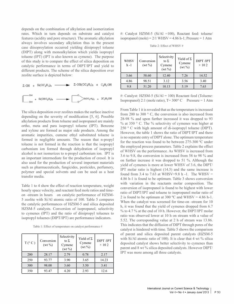
depends on the combination of alkylation and isomerization rates. Which in turn depends on substrate and catalyst features (acidity and pore structure). The aromatic alkylation always involves secondary alkylation thus in the present case diisoproylation occurred yielding diisipropyl toluene (DIPT) along with monoalkylation which yields isopropyl toluene (IPT) (IPT is also known as cymene). The purpose of this study is to compare the effect of silica deposition on catalytic performance in terms of DIPT/IPT and yield to different products. The scheme of the silica deposition over zeolite surface is depicted below:
The silica deposition over zeolites makes the surface inactive depending on the severity of modification [5, 6]. Possible alkylation products from toluene and isopropanol are mainly ortho, meta and para isopropyl toluene (IPT). Benzene and xylene are formed as major side products. Among the aromatic impurities, cumene ethyl substituted toluene is formed in negligible amounts. The reason that n-propyl toluene is not formed in the reaction is that the isopropyl carbonium ion formed through dehydration of isopropyl alcohol is not isomerizes to n-propyl carbonium ion. IPT is an important intermediate for the production of cresol. It is also used for the production of several important materials such as pharmaceuticals, fungicides, pesticides, perfumery, polymer and special solvents and can be used as a heat transfer media.
Table 1 to 4 show the effect of reaction temperature, weight hourly space velocity, and reactant feed mole ratios and time-on -stream in hours on catalytic performance of HZSM-5 zeolite with Si/Al atomic ratio of 100. Table 5 compares the catalytic performances of HZSM-5 and silica deposited HZSM-5 catalysts. Conversion of isopropanol, selectivity to cymenes (IPT) and the ratio of diisipropyl toluenes to isopropyl toluenes (DIPT/IPT) are performance indicators.
Table 1: Effect of temperature on catalyst performance #
T (° C ) Conversion (wt %)
Selectivity to Σ
Cymene (wt %)
Yield of Σ Cymene (wt %)
DIPT /IPT × 10 2
200 28.17 2.79 0.78 2.17250 93.77 3.90 3.65 14.23300 98.00 3.60 3.50 3.41350 93.47 4.20 2.93 12.6
#: Catalyst HZSM-5 (Si/Al =100), Reactant feed: toluene/isopropanol (mole) = 2/1 WHSV = 4.86 h-1; Pressure = 1 Atm
Table 2: Effect of WHSV #
WHSV h -1
Conversion (wt %)
Selectivity to Σ
Cymene (wt %)
Yield of Σ Cymene (wt %)
DIPT /IPT × 10 2
3.66 58.60 12.40 7.26 14.524.86 98.51 3.12 3.56 3.409.8 51.20 10.13 5.19 7.63
#: Catalyst: HZSM-5 (Si/Al = 100) Reactant feed (Toluene: Isopropanol) 2:1 (mole ratio), T= 300° C Pressure = 1 Atm
From Table 1 it is revealed that as the temperature is increased from 200 to 300 ° C, the conversion is also increased from 28-98 % and upon further increased it was dropped to 93 % at 350 ° C. The % selectivity of cymenes was higher at 250 º C with high amount of di-isopropyl toluene (DIPT). However, the table 1 shows the ratio of DIPT/IPT and there is no separate entry of DIPT alone. The optimum temperature for the reaction was found to be between 275-300 ºC under the employed process parameters. Table 2 explains the effect of WHSV on the performance. As WHSV is increased from 3.6 to 9.8, the conversion is increased from 58 to 98 % and on further increase it was dropped to 51 %. Although the yield of cymenes is more at lower WHSV of 3.6, the DIPT/IPT molar ratio is highest (14.5) and the same increase is found from 3.4 to 7.63 at WHSV=9.8 h -1. The WHSV = 4.86 h-1 is found to be optimum. Table 3 shows conversion with variation in the reactants molar composition. The conversion of isopropanol is found to be highest with lower ratio of DIPT/IPT and toluene to isopropanol molar ratio of 2 is found to be optimum at 300 ºC and WHSV = 4.86 h-1. When the catalyst was screened for time-on -stream for 10 h, it was found that the yield of cymenes dropped from 6.7 % to 4.7 % at the end of 10 h. However, the DIPT/IPT molar ratio was observed lower at 10 h on stream with a value of 5.52. The corresponding value at 2 h of stream was 13.86. This indicates that the diffusion of DIPT through pores of the catalyst is hindered with time. Table 5 shows the comparison of parent and silica deposited parent catalysts (HZSM-5 with Si/Al atomic ratio of 100). It is clear that 4 wt % silica deposited catalyst shows better selectivity to cymenes than parent and 8 wt % silica deposited catalysts. However DIPT/IPT was more among all three catalysts.
P 93International Journal on Current Science & Technology
Vol - I l No- I l January-June’2013
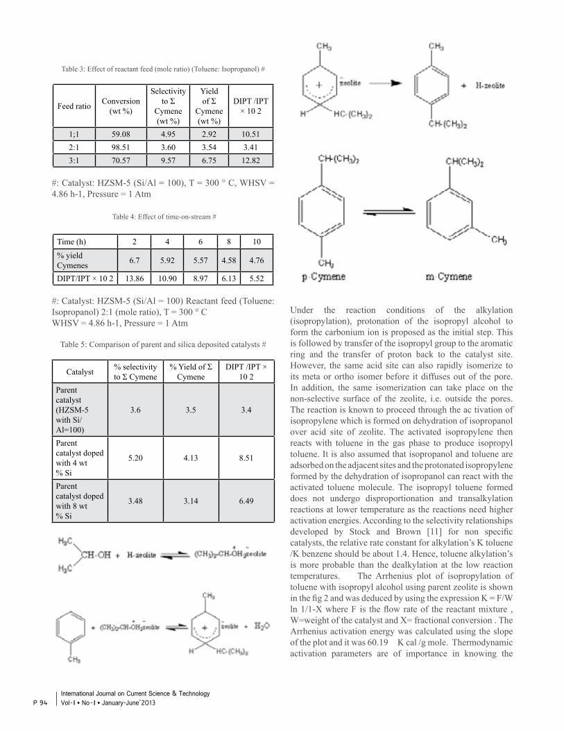
Table 3: Effect of reactant feed (mole ratio) (Toluene: Isopropanol) #
Feed ratio Conversion (wt %)
Selectivity to Σ
Cymene (wt %)
Yield of Σ
Cymene (wt %)
DIPT /IPT × 10 2
1;1 59.08 4.95 2.92 10.512:1 98.51 3.60 3.54 3.413:1 70.57 9.57 6.75 12.82
#: Catalyst: HZSM-5 (Si/Al = 100), T = 300 ° C, WHSV = 4.86 h-1, Pressure = 1 Atm
Table 4: Effect of time-on-stream #
Time (h) 2 4 6 8 10
% yield Cymenes 6.7 5.92 5.57 4.58 4.76
DIPT/IPT × 10 2 13.86 10.90 8.97 6.13 5.52
#: Catalyst: HZSM-5 (Si/Al = 100) Reactant feed (Toluene: Isopropanol) 2:1 (mole ratio), T = 300 ° C WHSV = 4.86 h-1, Pressure = 1 Atm
Table 5: Comparison of parent and silica deposited catalysts #
Catalyst % selectivity to Σ Cymene
% Yield of Σ Cymene
DIPT /IPT × 10 2
Parent catalyst (HZSM-5 with Si/Al=100)
3.6 3.5 3.4
Parent catalyst doped with 4 wt % Si
5.20 4.13 8.51
Parent catalyst doped with 8 wt % Si
3.48 3.14 6.49
#: Reactant feed (Toluene: Isopropanol) 2:1 (mole ratio), WHSV = 4.86 h-1, T = 300 ° C, Pressure = 1 Atm
Reaction scheme:
Fig 1: Reaction scheme of Isopropylation of toluene over zeolite catalyst
Under the reaction conditions of the alkylation (isopropylation), protonation of the isopropyl alcohol to form the carbonium ion is proposed as the initial step. This is followed by transfer of the isopropyl group to the aromatic ring and the transfer of proton back to the catalyst site. However, the same acid site can also rapidly isomerize to its meta or ortho isomer before it diffuses out of the pore. In addition, the same isomerization can take place on the non-selective surface of the zeolite, i.e. outside the pores. The reaction is known to proceed through the ac tivation of isopropylene which is formed on dehydration of isopropanol over acid site of zeolite. The activated isopropylene then reacts with toluene in the gas phase to produce isopropyl toluene. It is also assumed that isopropanol and toluene are adsorbed on the adjacent sites and the protonated isopropylene formed by the dehydration of isopropanol can react with the activated toluene molecule. The isopropyl toluene formed does not undergo disproportionation and transalkylation reactions at lower temperature as the reactions need higher activation energies. According to the selectivity relationships developed by Stock and Brown [11] for non specific catalysts, the relative rate constant for alkylation’s K toluene /K benzene should be about 1.4. Hence, toluene alkylation’s is more probable than the dealkylation at the low reaction temperatures. The Arrhenius plot of isopropylation of toluene with isopropyl alcohol using parent zeolite is shown in the fig 2 and was deduced by using the expression K = F/W ln 1/1-X where F is the flow rate of the reactant mixture , W=weight of the catalyst and X= fractional conversion . The Arrhenius activation energy was calculated using the slope of the plot and it was 60.19 K cal /g mole. Thermodynamic activation parameters are of importance in knowing the
P 94International Journal on Current Science & Technology Vol - I l No- I l January-June’2013
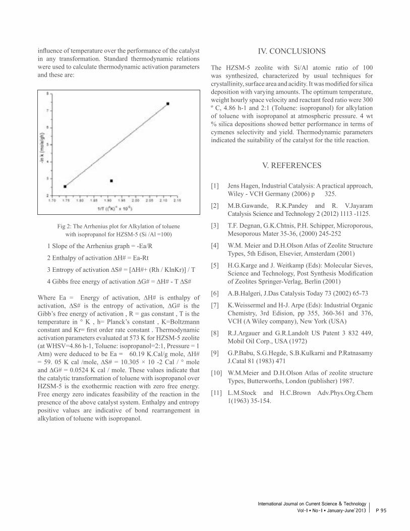
influence of temperature over the performance of the catalyst in any transformation. Standard thermodynamic relations were used to calculate thermodynamic activation parameters and these are:
Fig 2: The Arrhenius plot for Alkylation of toluenewith isopropanol for HZSM-5 (Si /Al =100)
1 Slope of the Arrhenius graph = -Ea/R
2 Enthalpy of activation ∆H# = Ea-Rt
3 Entropy of activation ∆S# = [∆H#+ (Rh / KlnKr)] / T
4 Gibbs free energy of activation ∆G# = ∆H# - T ∆S#
Where Ea = Energy of activation, ∆H# is enthalpy of activation, ∆S# is the entropy of activation, ∆G# is the Gibb’s free energy of activation , R = gas constant , T is the temperature in ° K , h= Planck’s constant , K=Boltzmann constant and Kr= first order rate constant . Thermodynamic activation parameters evaluated at 573 K for HZSM-5 zeolite (at WHSV=4.86 h-1, Toluene: isopropanol=2:1, Pressure = 1 Atm) were deduced to be Ea = 60.19 K.Cal/g mole, ∆H# = 59. 05 K cal /mole, ∆S# = 10.305 × 10 -2 Cal / ° mole and ∆G# = 0.0524 K cal / mole. These values indicate that the catalytic transformation of toluene with isopropanol over HZSM-5 is the exothermic reaction with zero free energy. Free energy zero indicates feasibility of the reaction in the presence of the above catalyst system. Enthalpy and entropy positive values are indicative of bond rearrangement in alkylation of toluene with isopropanol.
IV. CONCLUSIONS
The HZSM-5 zeolite with Si/Al atomic ratio of 100 was synthesized, characterized by usual techniques for crystallinity, surface area and acidity. It was modified for silica deposition with varying amounts. The optimum temperature, weight hourly space velocity and reactant feed ratio were 300 º C, 4.86 h-1 and 2:1 (Toluene: isopropanol) for alkylation of toluene with isopropanol at atmospheric pressure. 4 wt % silica depositions showed better performance in terms of cymenes selectivity and yield. Thermodynamic parameters indicated the suitability of the catalyst for the title reaction.
V. REFERENCES
[1] Jens Hagen, Industrial Catalysis: A practical approach, Wiley - VCH Germany (2006) p 325.
[2] M.B.Gawande, R.K.Pandey and R. V.Jayaram Catalysis Science and Technology 2 (2012) 1113 -1125.
[3] T.F. Degnan, G.K.Chtnis, P.H. Schipper, Microporous, Mesoporous Mater 35-36, (2000) 245-252
[4] W.M. Meier and D.H.Olson Atlas of Zeolite Structure Types, 5th Edison, Elsevier, Amsterdam (2001)
[5] H.G.Karge and J. Weitkamp (Eds): Molecular Sieves, Science and Technology, Post Synthesis Modification of Zeolites Springer-Verlag, Berlin (2001)
[6] A.B.Halgeri, J.Das Catalysis Today 73 (2002) 65-73
[7] K.Weissermel and H-J. Arpe (Eds): Industrial Organic Chemistry, 3rd Edision, pp 355, 360-361 and 376, VCH (A Wiley company), New York (USA)
[8] R.J.Argauer and G.R.Landolt US Patent 3 832 449, Mobil Oil Corp., USA (1972)
[9] G.P.Babu, S.G.Hegde, S.B.Kulkarni and P.Ratnasamy J.Catal 81 (1983) 471
[10] W.M.Meier and D.H.Olson Atlas of zeolite structure Types, Butterworths, London (publisher) 1987.
[11] L.M.Stock and H.C.Brown Adv.Phys.Org.Chem 1(1963) 35-154.
P 95International Journal on Current Science & Technology
Vol - I l No- I l January-June’2013

P 96International Journal on Current Science & Technology Vol - I l No- I l January-June’2013
MULTICHANNEL TRANSCEIVER SYSTEMDESIGN USING UNCOORDINATED DIRECT
SEQUENCE SPREAD SPECTRUM
S.Kalita, R.Kaushik, M.Jajoo, P.P.Sahu
Dept.of Electronics and Communication EngineeringTezpur University, Napaam
E-mail : [email protected]
ABSTRACT
In this paper, we have proposed and implemented a multichannel uncoordinated direct sequence spread spectrum (UDSSS) signaling scheme for underwater communication (UWC). In this scheme, the transmission of multichannel signal coded with pseudo-noise sequences in uncoordinated manner has been introduced. Because of using a set of shared keys and a randomizer in UDSSS transceiver system, it will increase the jamming resistance and security in underwater communication (UWC). We have shown bit error rate (BER) performance analysis by using circuit simulation model and from this it is seen that BER of the proposed circuit is less than that of the previous works.
Index Terms : UDSS ,UWC,BER,AWGN
I. NTRODUCTION
While wireless communication technology [1] today has become part of our daily life, the idea of wireless underwater communication may still seem far-fetched. However, research has been active for over a decade of designing the methods for wireless information transmission underwater. Human knowledge and understanding of the world under oceans, which constitute the major part of our planet, rests on our ability to collect information from remote undersea locations. The major discoveries of the past decades, such as the remains of the Titanic, or the hydro-thermal events at bottom of Deep Ocean, were made using cabled submersibles. Although such systems remain indispensable if high-speed communication link is to exist between the remote end and the surface, it is natural to wonder what one could accomplish without the burden (and cost) of heavy cables. Together with sensor technology and vehicular technology, wireless communications will enable new applications ranging from environmental monitoring to the gathering of oceanographic data, marine archaeology, and search and rescue missions.The signals that are used to carry digital information through
an underwater channel are not radio frequency (RF) signals, as electro-magnetic waves propagate only over extremely short distances due to having higher propagation loss. Here, acoustic waves are used, which can propagate over long distances. But due to having a multipath propagation and Doppler spread UWA communication is one of the most challenging transmission [2]. The equalizers have been used adaptively by previous authors to track potentially time varying Doppler shift [3].
With the rise of wireless communication technology the security and privacy of transmission become a major concern for not only military applications but also for commercial applications. To hide the transmitted information from malicious receiver and to overcome the jamming environment, the spread spectrum technique [4], has gained a great deal of prominence. For the safety issue under threat of jamming attackers in DSSS system an uncoordinated DSSS system is proposed by previous authors [5] in wireless communication.
In this paper, we have proposed and implemented an uncoordinated direct sequence spread spectrum (UDSSS) technique in DSSS signaling for multichannel in the UWC. For reduction of signal distortion due to multipath propagation and additive white Gaussian noise (AWGN) , correlators have been used with code hopping system.
II. MULTICHANNEL UDSSS TRANSCEIVER
The block diagram of the transmitter and receiver is given below in fig :1 (a) and fig:1 (b). In this scheme the data from each channel (total 4 channels) is grouped into 4-bit data word and one group are known as one symbol. So there will be 16 possible symbols of data. To spread these symbols in an uncoordinated way, 4 independent PN sequences of length 15 bits are used. Each of these PN-Sequences are shifted in phase using shift registers to get 15 sequences out of the same PN-sequence. Thus, we get 60 PN-sequences from 4 independent
P 97International Journal on Current Science & Technology
Vol - I l No- I l January-June’2013
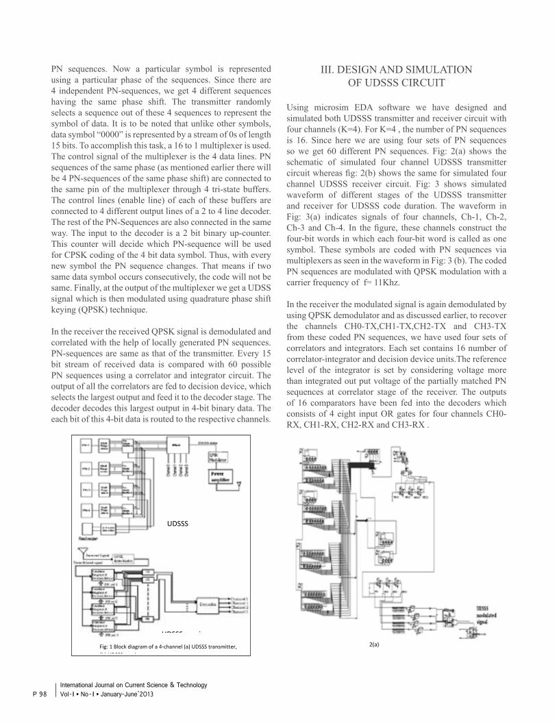
PN sequences. Now a particular symbol is represented using a particular phase of the sequences. Since there are 4 independent PN-sequences, we get 4 different sequences having the same phase shift. The transmitter randomly selects a sequence out of these 4 sequences to represent the symbol of data. It is to be noted that unlike other symbols, data symbol “0000” is represented by a stream of 0s of length 15 bits. To accomplish this task, a 16 to 1 multiplexer is used. The control signal of the multiplexer is the 4 data lines. PN sequences of the same phase (as mentioned earlier there will be 4 PN-sequences of the same phase shift) are connected to the same pin of the multiplexer through 4 tri-state buffers. The control lines (enable line) of each of these buffers are connected to 4 different output lines of a 2 to 4 line decoder. The rest of the PN-Sequences are also connected in the same way. The input to the decoder is a 2 bit binary up-counter. This counter will decide which PN-sequence will be used for CPSK coding of the 4 bit data symbol. Thus, with every new symbol the PN sequence changes. That means if two same data symbol occurs consecutively, the code will not be same. Finally, at the output of the multiplexer we get a UDSS signal which is then modulated using quadrature phase shift keying (QPSK) technique.
In the receiver the received QPSK signal is demodulated and correlated with the help of locally generated PN sequences. PN-sequences are same as that of the transmitter. Every 15 bit stream of received data is compared with 60 possible PN sequences using a correlator and integrator circuit. The output of all the correlators are fed to decision device, which selects the largest output and feed it to the decoder stage. The decoder decodes this largest output in 4-bit binary data. The each bit of this 4-bit data is routed to the respective channels.
UDSSS receiver Fig: 1 Block diagram of a 4-channel (a) UDSSS transmitter, (b) UDSSS receiver
UDSSS transmitter
III. DESIGN AND SIMULATIONOF UDSSS CIRCUIT
Using microsim EDA software we have designed and simulated both UDSSS transmitter and receiver circuit with four channels (K=4). For K=4 , the number of PN sequences is 16. Since here we are using four sets of PN sequences so we get 60 different PN sequences. Fig: 2(a) shows the schematic of simulated four channel UDSSS transmitter circuit whereas fig: 2(b) shows the same for simulated four channel UDSSS receiver circuit. Fig: 3 shows simulated waveform of different stages of the UDSSS transmitter and receiver for UDSSS code duration. The waveform in Fig: 3(a) indicates signals of four channels, Ch-1, Ch-2, Ch-3 and Ch-4. In the figure, these channels construct the four-bit words in which each four-bit word is called as one symbol. These symbols are coded with PN sequences via multiplexers as seen in the waveform in Fig: 3 (b). The coded PN sequences are modulated with QPSK modulation with a carrier frequency of f= 11Khz.
In the receiver the modulated signal is again demodulated by using QPSK demodulator and as discussed earlier, to recover the channels CH0-TX,CH1-TX,CH2-TX and CH3-TX from these coded PN sequences, we have used four sets of correlators and integrators. Each set contains 16 number of correlator-integrator and decision device units.The reference level of the integrator is set by considering voltage more than integrated out put voltage of the partially matched PN sequences at correlator stage of the receiver. The outputs of 16 comparators have been fed into the decoders which consists of 4 eight input OR gates for four channels CH0-RX, CH1-RX, CH2-RX and CH3-RX .
2(a)
P 98International Journal on Current Science & Technology Vol - I l No- I l January-June’2013
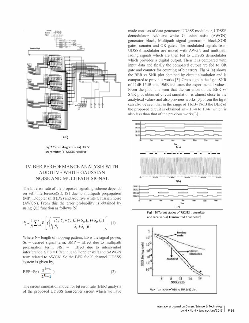
IV. BER PERFORMANCE ANALYSIS WITH ADDITIVE WHITE GAUSSIAN
NOISE AND MULTIPATH SIGNAL
The bit error rate of the proposed signaling scheme depends on self interference(SI), ISI due to multipath propagation (MP), Doppler shift (DS) and Additive white Gaussian noise (AWGN). From this the error probability is obtained by using Q(.) function as follows [5] (1)
Where N= length of hopping pattern, Eb is the signal power, Ss = desired signal term, SMP = Effect due to multipath propagation term, SISI = Effect due to intersymbol interference, SDS = Effect due to Doppler shift and SAWGN term related to AWGN. So the BER for K channel UDSSS system is given by,
BER=Pe ( ) (2)
The circuit simulation model for bit error rate (BER) analysis of the proposed UDSSS transceiver circuit which we have
∑ −
=
++++
=1
00 )(
)()()(21 N
enS
DSISIMPSbe SS
SSSSNE
QEN
Pµ µ
µµµ
made consists of data generator, UDSSS modulator, UDSSS demodulator, Additive white Gaussian noise (AWGN) generator block, Multipath signal generation block,XOR gates, counter and OR gates. The modulated signals from UDSSS modulator are mixed with AWGN and multipath fading signals which are then fed to UDSSS demodulator which provides a digital output. Then it is compared with input data and finally the compared output are fed to OR gate and counter for counting of bit errors. Fig :4 (a) shows the BER vs SNR plot obtained by circuit simulation and is compared to previous works [3]. Cross sign in the fig at SNR of 11dB,15dB and 19dB indicates the experimental values. From the plot it is seen that the variation of the BER vs SNR plot obtained circuit simulation is almost close to the analytical values and also previous works [3]. From the fig it can also be seen that in the range of 11dB~19dB the BER of the proposed circuit is obtained as ~ 10-4 to 10-6 which is also less than that of the previous works[3].
Fig:2 Circuit diagram of (a) UDSSS transmitter (b) UDSSS receiver
2(b)
Fig3: Different stages of UDSSS transmitter and receiver (a) Transmitted Channel (b) coded sequence with modulated waveform
Fig:4 Variation of BER vs SNR (dB) plot
3(a)
3(b)
3(c)
P 99International Journal on Current Science & Technology
Vol - I l No- I l January-June’2013
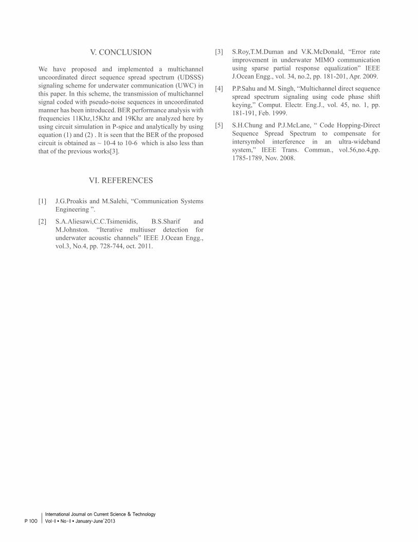
V. CONCLUSION
We have proposed and implemented a multichannel uncoordinated direct sequence spread spectrum (UDSSS) signaling scheme for underwater communication (UWC) in this paper. In this scheme, the transmission of multichannel signal coded with pseudo-noise sequences in uncoordinated manner has been introduced. BER performance analysis with frequencies 11Khz,15Khz and 19Khz are analyzed here by using circuit simulation in P-spice and analytically by using equation (1) and (2) . It is seen that the BER of the proposed circuit is obtained as ~ 10-4 to 10-6 which is also less than that of the previous works[3].
VI. REFERENCES
[1] J.G.Proakis and M.Salehi, “Communication Systems Engineering ”.
[2] S.A.Aliesawi,C.C.Tsimenidis, B.S.Sharif and M.Johnston. “Iterative multiuser detection for underwater acoustic channels” IEEE J.Ocean Engg., vol.3, No.4, pp. 728-744, oct. 2011.
[3] S.Roy,T.M.Duman and V.K.McDonald, “Error rate improvement in underwater MIMO communication using sparse partial response equalization” IEEE J.Ocean Engg., vol. 34, no.2, pp. 181-201, Apr. 2009.
[4] P.P.Sahu and M. Singh, “Multichannel direct sequence spread spectrum signaling using code phase shift keying,” Comput. Electr. Eng.J., vol. 45, no. 1, pp. 181-191, Feb. 1999.
[5] S.H.Chung and P.J.McLane, “ Code Hopping-Direct Sequence Spread Spectrum to compensate for intersymbol interference in an ultra-wideband system,” IEEE Trans. Commun., vol.56,no.4,pp. 1785-1789, Nov. 2008.
P 100International Journal on Current Science & Technology Vol - I l No- I l January-June’2013
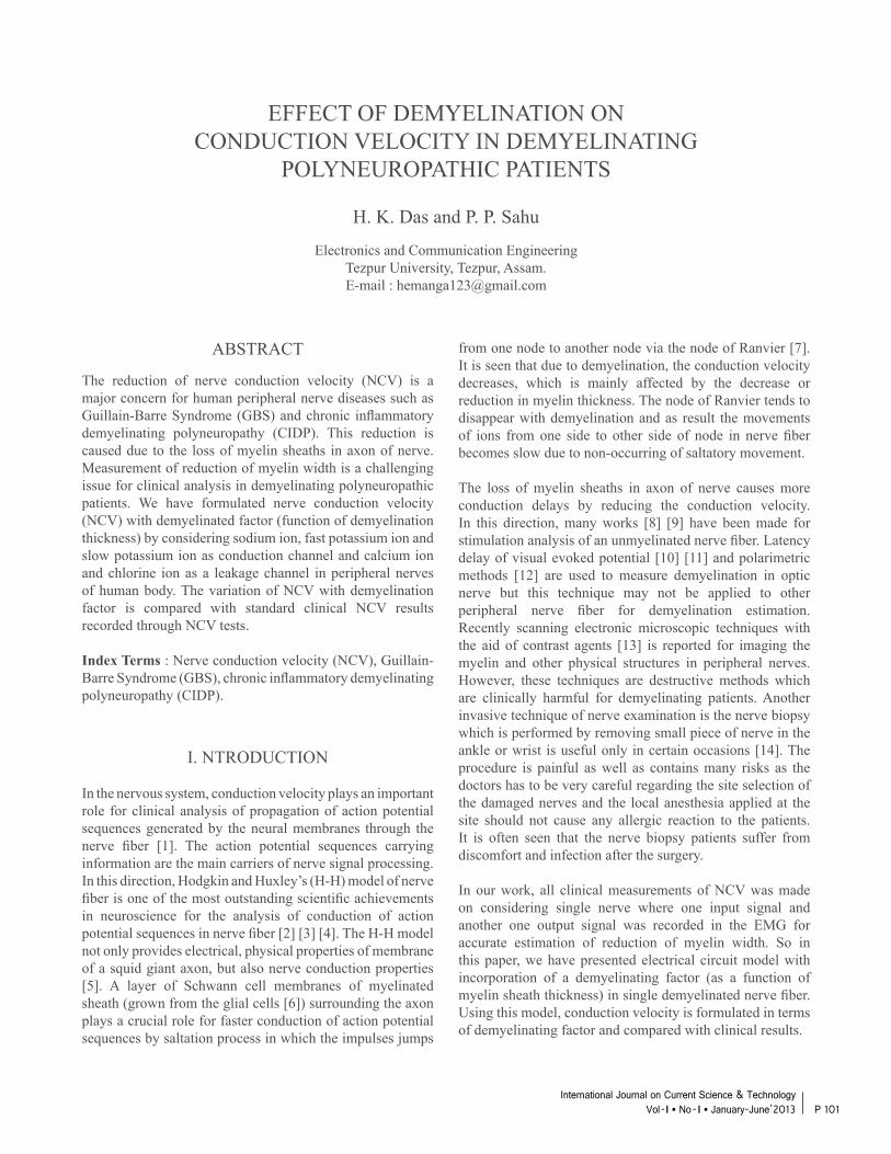
EFFECT OF DEMYELINATION ONCONDUCTION VELOCITY IN DEMYELINATING
POLYNEUROPATHIC PATIENTS
H. K. Das and P. P. Sahu
Electronics and Communication EngineeringTezpur University, Tezpur, Assam.E-mail : [email protected]
ABSTRACT
The reduction of nerve conduction velocity (NCV) is a major concern for human peripheral nerve diseases such as Guillain-Barre Syndrome (GBS) and chronic inflammatory demyelinating polyneuropathy (CIDP). This reduction is caused due to the loss of myelin sheaths in axon of nerve. Measurement of reduction of myelin width is a challenging issue for clinical analysis in demyelinating polyneuropathic patients. We have formulated nerve conduction velocity (NCV) with demyelinated factor (function of demyelination thickness) by considering sodium ion, fast potassium ion and slow potassium ion as conduction channel and calcium ion and chlorine ion as a leakage channel in peripheral nerves of human body. The variation of NCV with demyelination factor is compared with standard clinical NCV results recorded through NCV tests.
Index Terms : Nerve conduction velocity (NCV), Guillain-Barre Syndrome (GBS), chronic inflammatory demyelinating polyneuropathy (CIDP).
I. NTRODUCTION
In the nervous system, conduction velocity plays an important role for clinical analysis of propagation of action potential sequences generated by the neural membranes through the nerve fiber [1]. The action potential sequences carrying information are the main carriers of nerve signal processing. In this direction, Hodgkin and Huxley’s (H-H) model of nerve fiber is one of the most outstanding scientific achievements in neuroscience for the analysis of conduction of action potential sequences in nerve fiber [2] [3] [4]. The H-H model not only provides electrical, physical properties of membrane of a squid giant axon, but also nerve conduction properties [5]. A layer of Schwann cell membranes of myelinated sheath (grown from the glial cells [6]) surrounding the axon plays a crucial role for faster conduction of action potential sequences by saltation process in which the impulses jumps
from one node to another node via the node of Ranvier [7]. It is seen that due to demyelination, the conduction velocity decreases, which is mainly affected by the decrease or reduction in myelin thickness. The node of Ranvier tends to disappear with demyelination and as result the movements of ions from one side to other side of node in nerve fiber becomes slow due to non-occurring of saltatory movement.
The loss of myelin sheaths in axon of nerve causes more conduction delays by reducing the conduction velocity. In this direction, many works [8] [9] have been made for stimulation analysis of an unmyelinated nerve fiber. Latency delay of visual evoked potential [10] [11] and polarimetric methods [12] are used to measure demyelination in optic nerve but this technique may not be applied to other peripheral nerve fiber for demyelination estimation. Recently scanning electronic microscopic techniques with the aid of contrast agents [13] is reported for imaging the myelin and other physical structures in peripheral nerves. However, these techniques are destructive methods which are clinically harmful for demyelinating patients. Another invasive technique of nerve examination is the nerve biopsy which is performed by removing small piece of nerve in the ankle or wrist is useful only in certain occasions [14]. The procedure is painful as well as contains many risks as the doctors has to be very careful regarding the site selection of the damaged nerves and the local anesthesia applied at the site should not cause any allergic reaction to the patients. It is often seen that the nerve biopsy patients suffer from discomfort and infection after the surgery.
In our work, all clinical measurements of NCV was made on considering single nerve where one input signal and another one output signal was recorded in the EMG for accurate estimation of reduction of myelin width. So in this paper, we have presented electrical circuit model with incorporation of a demyelinating factor (as a function of myelin sheath thickness) in single demyelinated nerve fiber. Using this model, conduction velocity is formulated in terms of demyelinating factor and compared with clinical results.
P 101International Journal on Current Science & Technology
Vol - I l No- I l January-June’2013
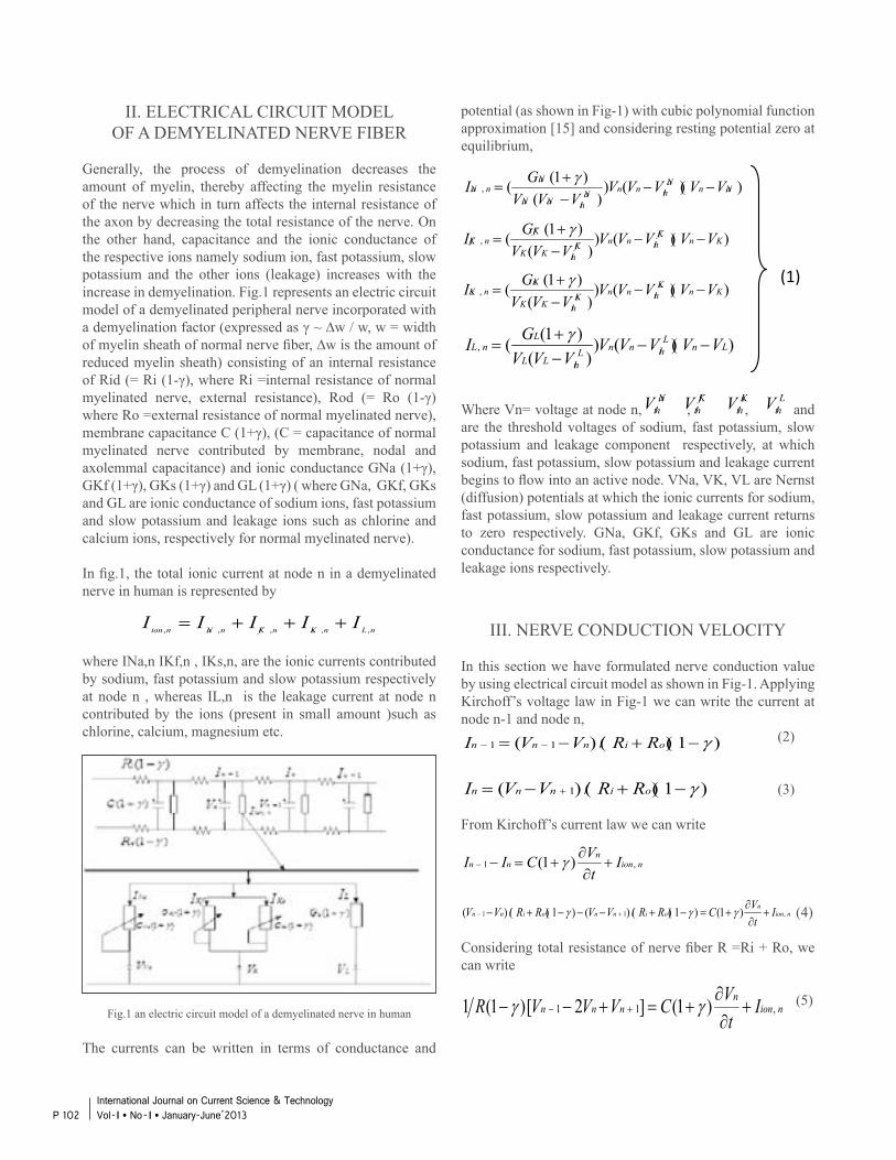
II. ELECTRICAL CIRCUIT MODELOF A DEMYELINATED NERVE FIBER
Generally, the process of demyelination decreases the amount of myelin, thereby affecting the myelin resistance of the nerve which in turn affects the internal resistance of the axon by decreasing the total resistance of the nerve. On the other hand, capacitance and the ionic conductance of the respective ions namely sodium ion, fast potassium, slow potassium and the other ions (leakage) increases with the increase in demyelination. Fig.1 represents an electric circuit model of a demyelinated peripheral nerve incorporated with a demyelination factor (expressed as γ ~ ∆w / w, w = width of myelin sheath of normal nerve fiber, ∆w is the amount of reduced myelin sheath) consisting of an internal resistance of Rid (= Ri (1-γ), where Ri =internal resistance of normal myelinated nerve, external resistance), Rod (= Ro (1-γ) where Ro =external resistance of normal myelinated nerve), membrane capacitance C (1+γ), (C = capacitance of normal myelinated nerve contributed by membrane, nodal and axolemmal capacitance) and ionic conductance GNa (1+γ), GKf (1+γ), GKs (1+γ) and GL (1+γ) ( where GNa, GKf, GKs and GL are ionic conductance of sodium ions, fast potassium and slow potassium and leakage ions such as chlorine and calcium ions, respectively for normal myelinated nerve).
In fig.1, the total ionic current at node n in a demyelinated nerve in human is represented by
where INa,n IKf,n , IKs,n, are the ionic currents contributed by sodium, fast potassium and slow potassium respectively at node n , whereas IL,n is the leakage current at node n contributed by the ions (present in small amount )such as chlorine, calcium, magnesium etc.
Fig.1 an electric circuit model of a demyelinated nerve in human
The currents can be written in terms of conductance and
nLnKsnKfnNanion IIIII ,,,,, +++=
potential (as shown in Fig-1) with cubic polynomial function approximation [15] and considering resting potential zero at equilibrium,
Where Vn= voltage at node n, , , and are the threshold voltages of sodium, fast potassium, slow potassium and leakage component respectively, at which sodium, fast potassium, slow potassium and leakage current begins to flow into an active node. VNa, VK, VL are Nernst (diffusion) potentials at which the ionic currents for sodium, fast potassium, slow potassium and leakage current returns to zero respectively. GNa, GKf, GKs and GL are ionic conductance for sodium, fast potassium, slow potassium and leakage ions respectively.
III. NERVE CONDUCTION VELOCITY
In this section we have formulated nerve conduction value by using electrical circuit model as shown in Fig-1. Applying Kirchoff’s voltage law in Fig-1 we can write the current at node n-1 and node n, (2)
(3)
From Kirchoff’s current law we can write
(4)
Considering total resistance of nerve fiber R =Ri + Ro, we can write
(5)
))(())(
)1((, NanNa
thnnNathNaNa
NanNa VVVVV
VVVGI −−
−+
=γ
))(())(
)1((, KnKf
thnnKfthKK
KfnKf VVVVV
VVVGI −−
−+
=γ
))(())(
)1((, KnKs
thnnKsthKK
KsnKs VVVVV
VVVGI −−
−+
=γ
))(())(
)1((, LnL
thnnLthLL
LnL VVVVV
VVVGI −−
−+
=γ
(1)
NathV Kf
thV KsthV L
thV
)1)(/()( 11 γ−+−= −− oinnn RRVVI
)1)(/()( 1 γ−+−= + oinnn RRVVI
nionn
nn It
VCII ,1 )1( +∂∂
+=−− γ
nionn
oinnoinn It
VCRRVVRRVV ,11 )1()1)(/()()1)(/()( +∂∂
+=−+−−−+− +− γγγ
nionn
nnn It
VCVVVR ,11 )1(]2[)1(1 +∂∂
+=+−− +− γγ
P 102International Journal on Current Science & Technology Vol - I l No- I l January-June’2013
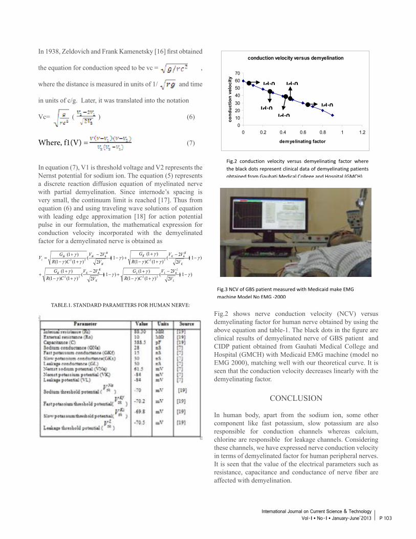
In 1938, Zeldovich and Frank Kamenetsky [16] first obtained
the equation for conduction speed to be vc = ,
where the distance is measured in units of 1/ and time
in units of c/g. Later, it was translated into the notation
Vc= ( ) (6)
Where, f1(V) = (7)
In equation (7), V1 is threshold voltage and V2 represents the Nernst potential for sodium ion. The equation (5) represents a discrete reaction diffusion equation of myelinated nerve with partial demyelination. Since internode’s spacing is very small, the continuum limit is reached [17]. Thus from equation (6) and using traveling wave solutions of equation with leading edge approximation [18] for action potential pulse in our formulation, the mathematical expression for conduction velocity incorporated with the demyelinated factor for a demyelinated nerve is obtained as
TABLE.1. STANDARD PARAMETERS FOR HUMAN NERVE:
)1)(2
2(
)1()1()1()1)(
22
()1()1(
)1(
)1)(2
2(
)1()1()1(
)1)(2
2(
)1()1()1(
2222
2222
γγγ
γγ
γγγ
γγγ
γγ
γγγ
−−
+−+
+−−
+−+
+
−−
+−
++−
−+−
+=
L
LthLL
K
KsthKKs
K
KfthKKf
Na
NathNaNa
c
VVV
CRG
VVV
CRG
VVV
CRG
VVV
CRG
V
Fig.2 shows nerve conduction velocity (NCV) versus demyelinating factor for human nerve obtained by using the above equation and table-1. The black dots in the figure are clinical results of demyelinated nerve of GBS patient and CIDP patient obtained from Gauhati Medical College and Hospital (GMCH) with Medicaid EMG machine (model no EMG 2000), matching well with our theoretical curve. It is seen that the conduction velocity decreases linearly with the demyelinating factor.
CONCLUSION
In human body, apart from the sodium ion, some other component like fast potassium, slow potassium are also responsible for conduction channels whereas calcium, chlorine are responsible for leakage channels. Considering these channels, we have expressed nerve conduction velocity in terms of demyelinated factor for human peripheral nerves. It is seen that the value of the electrical parameters such as resistance, capacitance and conductance of nerve fiber are affected with demyelination.
conduction velocity versus demyelination
010203040506070
0 0.2 0.4 0.6 0.8 1 1.2
demyelinating factor
cond
uctio
n ve
loci
ty
Id:083
Id:081
Id:032
Id:058
Id:047
Fig.2 conduction velocity versus demyelinating factor where the black dots represent clinical data of demyelinating patients obtained from Gauhati Medical College and Hospital (GMCH)
Fig.3 NCV of GBS patient measured with Medicaid make EMG machine Model No EMG -2000
P 103International Journal on Current Science & Technology
Vol - I l No- I l January-June’2013
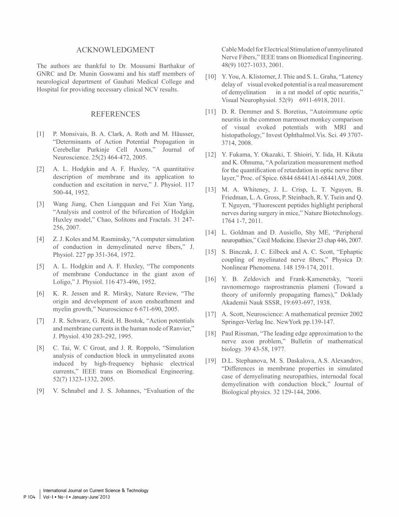
ACKNOWLEDGMENT
The authors are thankful to Dr. Mousumi Barthakur of GNRC and Dr. Munin Goswami and his staff members of neurological department of Gauhati Medical College and Hospital for providing necessary clinical NCV results.
REFERENCES
[1] P. Monsivais, B. A. Clark, A. Roth and M. Häusser, “Determinants of Action Potential Propagation in Cerebellar Purkinje Cell Axons,” Journal of Neuroscience. 25(2) 464-472, 2005.
[2] A. L. Hodgkin and A. F. Huxley, “A quantitative description of membrane and its application to conduction and excitation in nerve,” J. Physiol. 117 500-44, 1952.
[3] Wang Jiang, Chen Liangquan and Fei Xian Yang, “Analysis and control of the bifurcation of Hodgkin Huxley model,” Chao, Solitons and Fractals. 31 247- 256, 2007.
[4] Z. J. Koles and M. Rasminsky, “A computer simulation of conduction in demyelinated nerve fibers,” J. Physiol. 227 pp 351-364, 1972.
[5] A. L. Hodgkin and A. F. Huxley, “The components of membrane Conductance in the giant axon of Loligo,” J. Physiol. 116 473-496, 1952.
[6] K. R. Jessen and R. Mirsky, Nature Review, “The origin and development of axon ensheathment and myelin growth,” Neuroscience 6 671-690, 2005.
[7] J. R. Schwarz, G. Reid, H. Bostok, “Action potentials and membrane currents in the human node of Ranvier,” J. Physiol. 430 283-292, 1995.
[8] C. Tai, W. C Groat, and J. R. Roppolo, “Simulation analysis of conduction block in unmyelinated axons induced by high-frequency biphasic electrical currents,” IEEE trans on Biomedical Engineering. 52(7) 1323-1332, 2005.
[9] V. Schnabel and J. S. Johannes, “Evaluation of the
Cable Model for Electrical Stimulation of unmyelinated Nerve Fibers,” IEEE trans on Biomedical Engineering. 48(9) 1027-1033, 2001.
[10] Y. You, A. Klistorner, J. Thie and S. L. Graha, “Latency delay of visual evoked potential is a real measurement of demyelination in a rat model of optic neuritis,” Visual Neurophysiol. 52(9) 6911-6918, 2011.
[11] D. R. Demmer and S. Boretius, “Autoimmune optic neuritis in the common marmoset monkey comparison of visual evoked potentials with MRI and histopathology,” Invest Ophthalmol.Vis. Sci. 49 3707- 3714, 2008.
[12] Y. Fukama, Y. Okazaki, T. Shioiri, Y. Iida, H. Kikuta and K. Ohnuma, “A polarization measurement method for the quantification of retardation in optic nerve fiber layer,” Proc. of Spice. 6844 68441A1-68441A9, 2008.
[13] M. A. Whiteney, J. L. Crisp, L. T. Nguyen, B. Friedman, L. A. Gross, P. Steinbach, R. Y. Tsein and Q. T. Nguyen, “Fluorescent peptides highlight peripheral nerves during surgery in mice,” Nature Biotechnology. 1764 1-7, 2011.
[14] L. Goldman and D. Ausiello, Shy ME, “Peripheral neuropathies,” Cecil Medicine. Elsevier 23 chap 446, 2007.
[15] S. Binczak, J. C. Eilbeck and A. C. Scott, “Ephaptic coupling of myelinated nerve fibers,” Physica D: Nonlinear Phenomena. 148 159-174, 2011.
[16] Y. B. Zeldovich and Frank-Kamenetsky, “teorii ravnomernogo rasprostranenia plameni (Toward a theory of uniformly propagating flames),” Doklady Akademii Nauk SSSR, 19:693-697, 1938.
[17] A. Scott, Neuroscience: A mathematical premier 2002 Springer-Verlag Inc. NewYork pp.139-147.
[18] Paul Rissman, “The leading edge approximation to the nerve axon problem,” Bulletin of mathematical biology. 39 43-58, 1977.
[19] D.L. Stephanova, M. S. Daskalova, A.S. Alexandrov, “Differences in membrane properties in simulated case of demyelinating neuropathies, internodal focal demyelination with conduction block,” Journal of Biological physics. 32 129-144, 2006.
P 104International Journal on Current Science & Technology Vol - I l No- I l January-June’2013
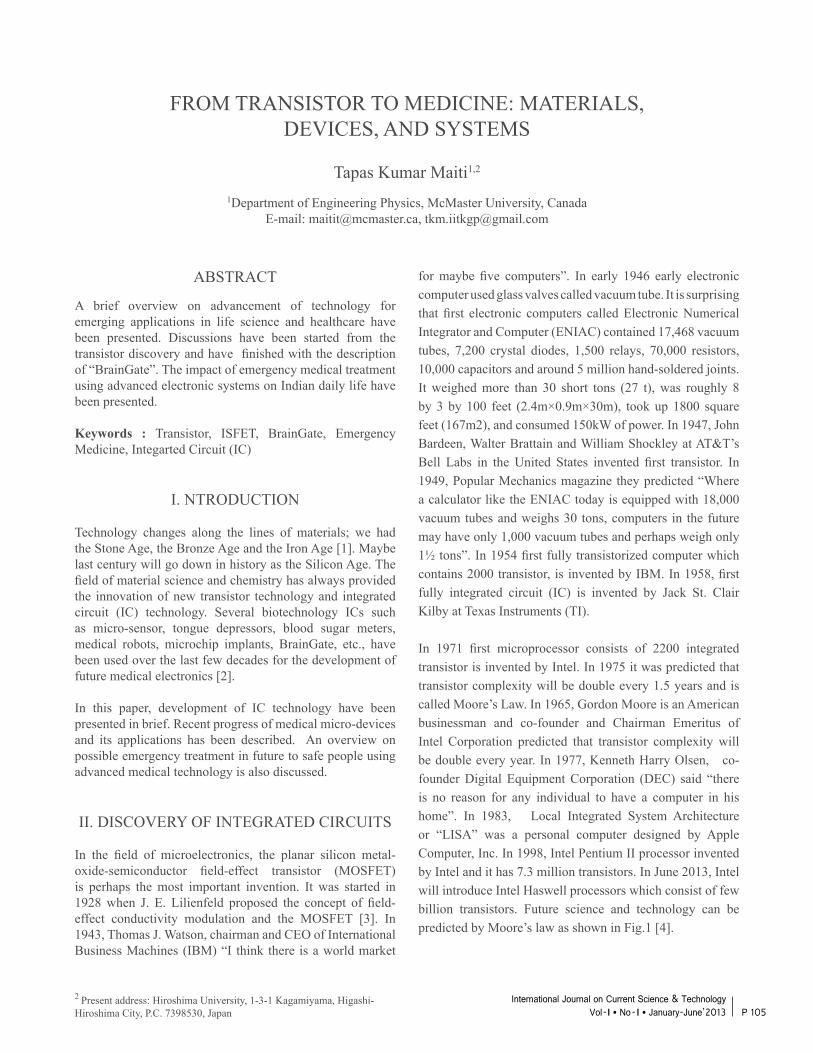
FROM TRANSISTOR TO MEDICINE: MATERIALS, DEVICES, AND SYSTEMS
Tapas Kumar Maiti1,2
1Department of Engineering Physics, McMaster University, CanadaE-mail: [email protected], [email protected]
ABSTRACT
A brief overview on advancement of technology for emerging applications in life science and healthcare have been presented. Discussions have been started from the transistor discovery and have finished with the description of “BrainGate”. The impact of emergency medical treatment using advanced electronic systems on Indian daily life have been presented.
Keywords : Transistor, ISFET, BrainGate, Emergency Medicine, Integarted Circuit (IC)
I. NTRODUCTION
Technology changes along the lines of materials; we had the Stone Age, the Bronze Age and the Iron Age [1]. Maybe last century will go down in history as the Silicon Age. The field of material science and chemistry has always provided the innovation of new transistor technology and integrated circuit (IC) technology. Several biotechnology ICs such as micro-sensor, tongue depressors, blood sugar meters, medical robots, microchip implants, BrainGate, etc., have been used over the last few decades for the development of future medical electronics [2].
In this paper, development of IC technology have been presented in brief. Recent progress of medical micro-devices and its applications has been described. An overview on possible emergency treatment in future to safe people using advanced medical technology is also discussed.
II. DISCOVERY OF INTEGRATED CIRCUITS
In the field of microelectronics, the planar silicon metal-oxide-semiconductor field-effect transistor (MOSFET) is perhaps the most important invention. It was started in 1928 when J. E. Lilienfeld proposed the concept of field-effect conductivity modulation and the MOSFET [3]. In 1943, Thomas J. Watson, chairman and CEO of International Business Machines (IBM) “I think there is a world market
for maybe five computers”. In early 1946 early electronic computer used glass valves called vacuum tube. It is surprising that first electronic computers called Electronic Numerical Integrator and Computer (ENIAC) contained 17,468 vacuum tubes, 7,200 crystal diodes, 1,500 relays, 70,000 resistors, 10,000 capacitors and around 5 million hand-soldered joints. It weighed more than 30 short tons (27 t), was roughly 8 by 3 by 100 feet (2.4m×0.9m×30m), took up 1800 square feet (167m2), and consumed 150kW of power. In 1947, John Bardeen, Walter Brattain and William Shockley at AT&T’s Bell Labs in the United States invented first transistor. In 1949, Popular Mechanics magazine they predicted “Where a calculator like the ENIAC today is equipped with 18,000 vacuum tubes and weighs 30 tons, computers in the future may have only 1,000 vacuum tubes and perhaps weigh only 1½ tons”. In 1954 first fully transistorized computer which contains 2000 transistor, is invented by IBM. In 1958, first fully integrated circuit (IC) is invented by Jack St. Clair Kilby at Texas Instruments (TI).
In 1971 first microprocessor consists of 2200 integrated transistor is invented by Intel. In 1975 it was predicted that transistor complexity will be double every 1.5 years and is called Moore’s Law. In 1965, Gordon Moore is an American businessman and co-founder and Chairman Emeritus of Intel Corporation predicted that transistor complexity will be double every year. In 1977, Kenneth Harry Olsen, co-founder Digital Equipment Corporation (DEC) said “there is no reason for any individual to have a computer in his home”. In 1983, Local Integrated System Architecture or “LISA” was a personal computer designed by Apple Computer, Inc. In 1998, Intel Pentium II processor invented by Intel and it has 7.3 million transistors. In June 2013, Intel will introduce Intel Haswell processors which consist of few billion transistors. Future science and technology can be predicted by Moore’s law as shown in Fig.1 [4].
2 Present address: Hiroshima University, 1-3-1 Kagamiyama, Higashi-Hiroshima City, P.C. 7398530, Japan P 105
International Journal on Current Science & Technology Vol - I l No- I l January-June’2013
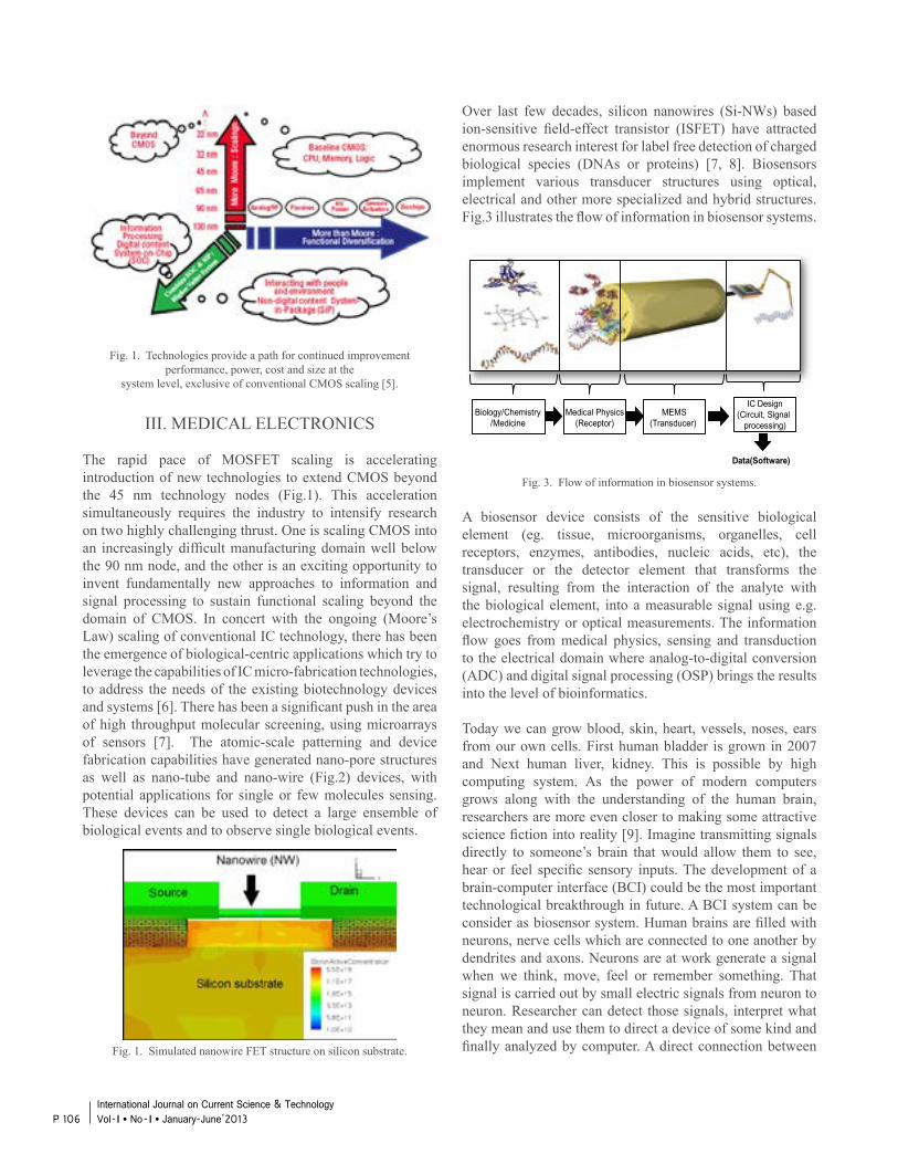
Over last few decades, silicon nanowires (Si-NWs) based ion-sensitive field-effect transistor (ISFET) have attracted enormous research interest for label free detection of charged biological species (DNAs or proteins) [7, 8]. Biosensors implement various transducer structures using optical, electrical and other more specialized and hybrid structures. Fig.3 illustrates the flow of information in biosensor systems.
Fig. 3. Flow of information in biosensor systems. A biosensor device consists of the sensitive biological element (eg. tissue, microorganisms, organelles, cell receptors, enzymes, antibodies, nucleic acids, etc), the transducer or the detector element that transforms the signal, resulting from the interaction of the analyte with the biological element, into a measurable signal using e.g. electrochemistry or optical measurements. The information flow goes from medical physics, sensing and transduction to the electrical domain where analog-to-digital conversion (ADC) and digital signal processing (OSP) brings the results into the level of bioinformatics.
Today we can grow blood, skin, heart, vessels, noses, ears from our own cells. First human bladder is grown in 2007 and Next human liver, kidney. This is possible by high computing system. As the power of modern computers grows along with the understanding of the human brain, researchers are more even closer to making some attractive science fiction into reality [9]. Imagine transmitting signals directly to someone’s brain that would allow them to see, hear or feel specific sensory inputs. The development of a brain-computer interface (BCI) could be the most important technological breakthrough in future. A BCI system can be consider as biosensor system. Human brains are filled with neurons, nerve cells which are connected to one another by dendrites and axons. Neurons are at work generate a signal when we think, move, feel or remember something. That signal is carried out by small electric signals from neuron to neuron. Researcher can detect those signals, interpret what they mean and use them to direct a device of some kind and finally analyzed by computer. A direct connection between
Fig. 1. Technologies provide a path for continued improvementperformance, power, cost and size at the
system level, exclusive of conventional CMOS scaling [5].
III. MEDICAL ELECTRONICS
The rapid pace of MOSFET scaling is accelerating introduction of new technologies to extend CMOS beyond the 45 nm technology nodes (Fig.1). This acceleration simultaneously requires the industry to intensify research on two highly challenging thrust. One is scaling CMOS into an increasingly difficult manufacturing domain well below the 90 nm node, and the other is an exciting opportunity to invent fundamentally new approaches to information and signal processing to sustain functional scaling beyond the domain of CMOS. In concert with the ongoing (Moore’s Law) scaling of conventional IC technology, there has been the emergence of biological-centric applications which try to leverage the capabilities of IC micro-fabrication technologies, to address the needs of the existing biotechnology devices and systems [6]. There has been a significant push in the area of high throughput molecular screening, using microarrays of sensors [7]. The atomic-scale patterning and device fabrication capabilities have generated nano-pore structures as well as nano-tube and nano-wire (Fig.2) devices, with potential applications for single or few molecules sensing. These devices can be used to detect a large ensemble of biological events and to observe single biological events.
Fig. 1. Simulated nanowire FET structure on silicon substrate.
Biology/Chemistry/Medicine
Medical Physics(Receptor)
MEMS(Transducer)
IC Design(Circuit, Signal
processing)
Data(Software)
P 106International Journal on Current Science & Technology Vol - I l No- I l January-June’2013
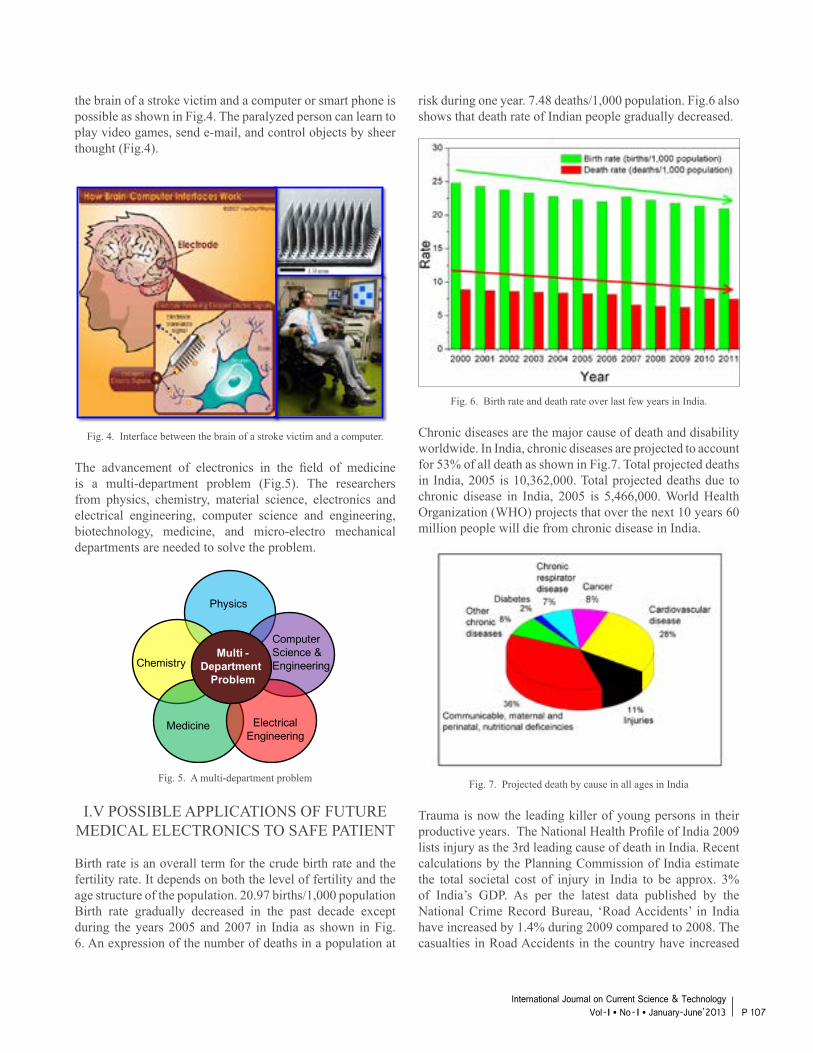
the brain of a stroke victim and a computer or smart phone is possible as shown in Fig.4. The paralyzed person can learn to play video games, send e-mail, and control objects by sheer thought (Fig.4).
Fig. 4. Interface between the brain of a stroke victim and a computer.
The advancement of electronics in the field of medicine is a multi-department problem (Fig.5). The researchers from physics, chemistry, material science, electronics and electrical engineering, computer science and engineering, biotechnology, medicine, and micro-electro mechanical departments are needed to solve the problem.
Fig. 5. A multi-department problem
I.V POSSIBLE APPLICATIONS OF FUTURE MEDICAL ELECTRONICS TO SAFE PATIENT
Birth rate is an overall term for the crude birth rate and the fertility rate. It depends on both the level of fertility and the age structure of the population. 20.97 births/1,000 population Birth rate gradually decreased in the past decade except during the years 2005 and 2007 in India as shown in Fig. 6. An expression of the number of deaths in a population at
Physics
Chemistry
Medicine ElectricalEngineering
Computer Science & Engineering
Multi -Department
Problem
risk during one year. 7.48 deaths/1,000 population. Fig.6 also shows that death rate of Indian people gradually decreased.
Fig. 6. Birth rate and death rate over last few years in India.
Chronic diseases are the major cause of death and disability worldwide. In India, chronic diseases are projected to account for 53% of all death as shown in Fig.7. Total projected deaths in India, 2005 is 10,362,000. Total projected deaths due to chronic disease in India, 2005 is 5,466,000. World Health Organization (WHO) projects that over the next 10 years 60 million people will die from chronic disease in India.
Fig. 7. Projected death by cause in all ages in India
Trauma is now the leading killer of young persons in their productive years. The National Health Profile of India 2009 lists injury as the 3rd leading cause of death in India. Recent calculations by the Planning Commission of India estimate the total societal cost of injury in India to be approx. 3% of India’s GDP. As per the latest data published by the National Crime Record Bureau, ‘Road Accidents’ in India have increased by 1.4% during 2009 compared to 2008. The casualties in Road Accidents in the country have increased
P 107International Journal on Current Science & Technology
Vol - I l No- I l January-June’2013
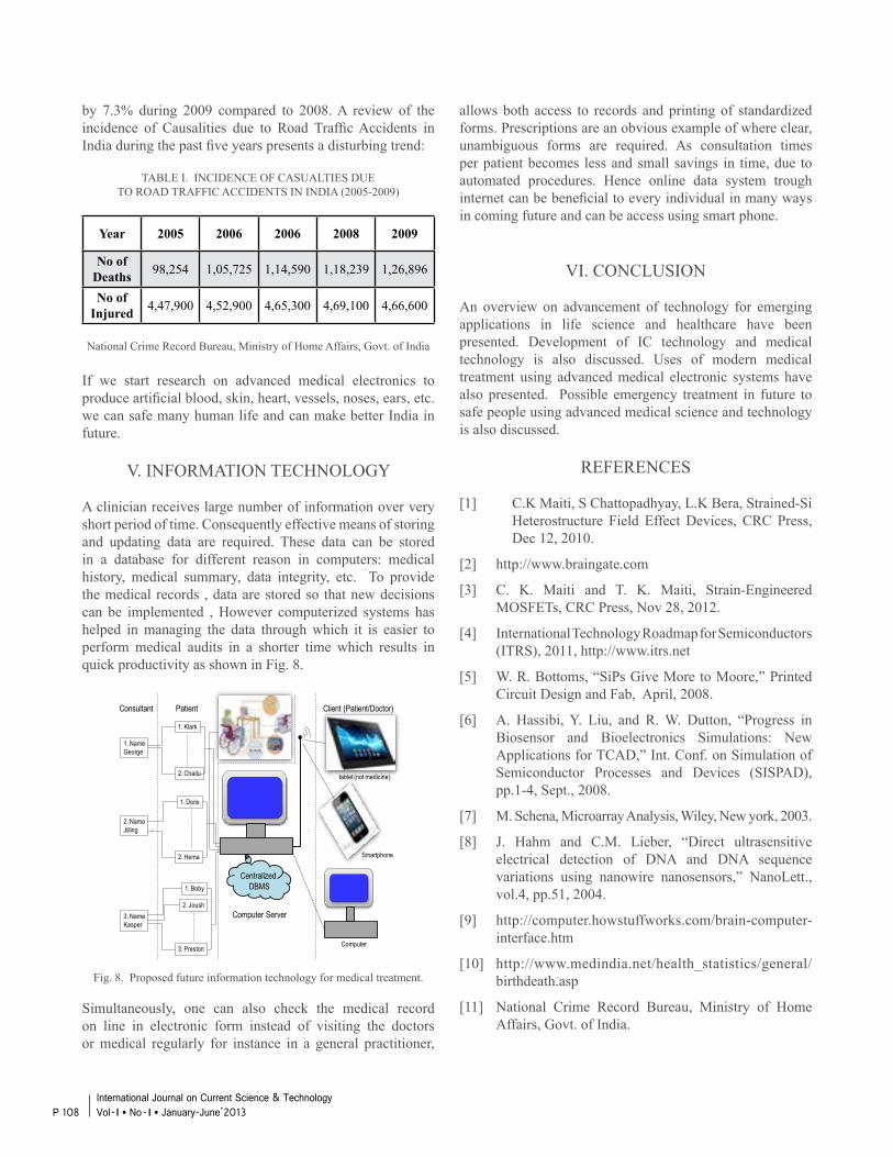
by 7.3% during 2009 compared to 2008. A review of the incidence of Causalities due to Road Traffic Accidents in India during the past five years presents a disturbing trend:
TABLE I. INCIDENCE OF CASUALTIES DUETO ROAD TRAFFIC ACCIDENTS IN INDIA (2005-2009)
Year 2005 2006 2006 2008 2009
No of Deaths 98,254 1,05,725 1,14,590 1,18,239 1,26,896
No of Injured 4,47,900 4,52,900 4,65,300 4,69,100 4,66,600
National Crime Record Bureau, Ministry of Home Affairs, Govt. of India
If we start research on advanced medical electronics to produce artificial blood, skin, heart, vessels, noses, ears, etc. we can safe many human life and can make better India in future.
V. INFORMATION TECHNOLOGY
A clinician receives large number of information over very short period of time. Consequently effective means of storing and updating data are required. These data can be stored in a database for different reason in computers: medical history, medical summary, data integrity, etc. To provide the medical records , data are stored so that new decisions can be implemented , However computerized systems has helped in managing the data through which it is easier to perform medical audits in a shorter time which results in quick productivity as shown in Fig. 8.
Fig. 8. Proposed future information technology for medical treatment.
Simultaneously, one can also check the medical record on line in electronic form instead of visiting the doctors or medical regularly for instance in a general practitioner,
Consultant
1. NameGeorge
2. NameJilling
3. NameKasper
Patient
1. Klark
2. Chaitu
1. Doris
2. Hema
1. Boby
2. Joush
3. Preston
Computer Server
Centralized DBMS
Client (Patient/Doctor)
Computer
Smartphone
tablet (not medicine)
allows both access to records and printing of standardized forms. Prescriptions are an obvious example of where clear, unambiguous forms are required. As consultation times per patient becomes less and small savings in time, due to automated procedures. Hence online data system trough internet can be beneficial to every individual in many ways in coming future and can be access using smart phone.
VI. CONCLUSION
An overview on advancement of technology for emerging applications in life science and healthcare have been presented. Development of IC technology and medical technology is also discussed. Uses of modern medical treatment using advanced medical electronic systems have also presented. Possible emergency treatment in future to safe people using advanced medical science and technology is also discussed.
REFERENCES
[1] C.K Maiti, S Chattopadhyay, L.K Bera, Strained-Si Heterostructure Field Effect Devices, CRC Press, Dec 12, 2010.
[2] http://www.braingate.com
[3] C. K. Maiti and T. K. Maiti, Strain-Engineered MOSFETs, CRC Press, Nov 28, 2012.
[4] International Technology Roadmap for Semiconductors (ITRS), 2011, http://www.itrs.net
[5] W. R. Bottoms, “SiPs Give More to Moore,” Printed Circuit Design and Fab, April, 2008.
[6] A. Hassibi, Y. Liu, and R. W. Dutton, “Progress in Biosensor and Bioelectronics Simulations: New Applications for TCAD,” Int. Conf. on Simulation of Semiconductor Processes and Devices (SISPAD), pp.1-4, Sept., 2008.
[7] M. Schena, Microarray Analysis, Wiley, New york, 2003.
[8] J. Hahm and C.M. Lieber, “Direct ultrasensitive electrical detection of DNA and DNA sequence variations using nanowire nanosensors,” NanoLett., vol.4, pp.51, 2004.
[9] http://computer.howstuffworks.com/brain-computer- interface.htm
[10] http://www.medindia.net/health_statistics/general/ birthdeath.asp
[11] National Crime Record Bureau, Ministry of Home Affairs, Govt. of India.
P 108International Journal on Current Science & Technology Vol - I l No- I l January-June’2013
ENZYME-MODIFIED FIELD EFFECT TRANSISTORS (ENFETS) AS BIOSENSORS : A RESEARCH REVIEW
Manoj Kumar Sarma1, Jiten Ch.Dutta2
1Department of Physics, Darrang College, Tezpur,2Department of Electronics and Communication Engineering
Tezpur University, Assam, IndiaEmail : [email protected], [email protected]
ABSTRACT
In recent years, increasing interest has been shown in the development of Bioelectronic sensors based on ion sensitive field effect transistors(ISFETs). Many ISFET based chemical sensors specially enzyme field effect transistors (ENFETs) have got a fare share for applications in the fields of medical, environmental, food safety, military and biotechnology areas. The growing interest for development of these sensors is due to the fact that they are manufactured by means of semiconductor technology which has already entered into multifunctional “more than more” regime that is increasingly multidisciplinary in nature. Technology involved has, therefore, innovative potential that may result in the appearance of new sensor and device technologies in future. The basic theoretical principles of enzyme field effect transistors (ENFETs), the operation principle of ENFET and a brief introduction of ENFET technology are considered in this paper.
Keywords : ISFET; Enzyme; pH; Biosensor.
I. NTRODUCTION
The ion sensitive field effect transistor, the heart of enzyme field effect transistor, was first reported by Bergveld in 1970, who used it for the measurement of ionic in and effluxes around a nerve [1]. This work was described in detail in 1972 [2], which is now cited by most authors as a pioneering publication in the field of ISFET development. At the same time Matsuo and Wise developed a similar device using silicon nitride as a sensitive sub gate layer, which greatly improved the sensor performance [3]. Since 1970, led by Bergveld, more than 600 papers, devoted on ISFETs [3-4], and another 170 on related biosensors , such as Enzyme FETs (ENFETs) [5-10], Immuno FETs (IMFETs) [11], DNA biosensor [12] etc., appeared in many world’s leading journals on biomedical, electron devices, sensors and actuators, biosensors and bioelectronics, biotechnology advances etc.
Enzyme-modified field effect transistor refers to a bioelectronic device which incorporates an enzyme system in conjunction with an ion sensitive field effect transistor (ISFET). Biocatalytic transformations stimulated by enzyme alter the pH at the gate surface of the ISFET either by consuming or generating protons. The change in pH inside the enzyme system affects the surface potential of the ISFET resulting into the change of channel current. Thus from the point of view of signal transduction, ENFET may be defined as an bioelectronic device which converts a biological or biochemical signal into an electrical signal. In ENFET device, enzyme system acts as a bioreceptors which recognizes a biological event and then through biocatalytic reaction transforms it into quantity detectable by an underlying ISFET. This idea was first given by Janata and Moss in 1976 [13], but till 1980, no one was able to give accepted results related to this idea. In 1980, Caras and J. Janata presented the first results regarding ISFET based penicillin sensor [14]. The device that they described consisted of two ISFETs, one of which had on the top of the gate surface a membrane with covalently bound penicillinase enzyme and albumin, while the other had on the top of the gate surface a membrane with only covalently bound albumin. Basic principle is that when penicillin was present in solution, penicillinase enzyme in the membrane catalyzed penicillin that resulted in the production of protons and therefore a local pH decreases in the gate area of the ISFET resulting into an increased drain current registered by the ISFET.
After this publication, two important research works related with ISFET based sensors were presented at the first international conference on chemical sensors held in 1983 in Fukuoka, Japan. ISFET for urea and acetylcholine determination by Y. Miahara et al. [15] and ENFET for glucose determination by Y. Hanazato and S. Shiono [16]. After these developments, more than 150 publications developed to various aspects of ENFET development and operation have appeared in many world’s leading journals published by IEEE, ELSEVIER etc. [17]. In recent years much attention has been paid to the development of these devices because they are manufactured by means of these
P 109International Journal on Current Science & Technology
Vol - I l No- I l January-June’2013
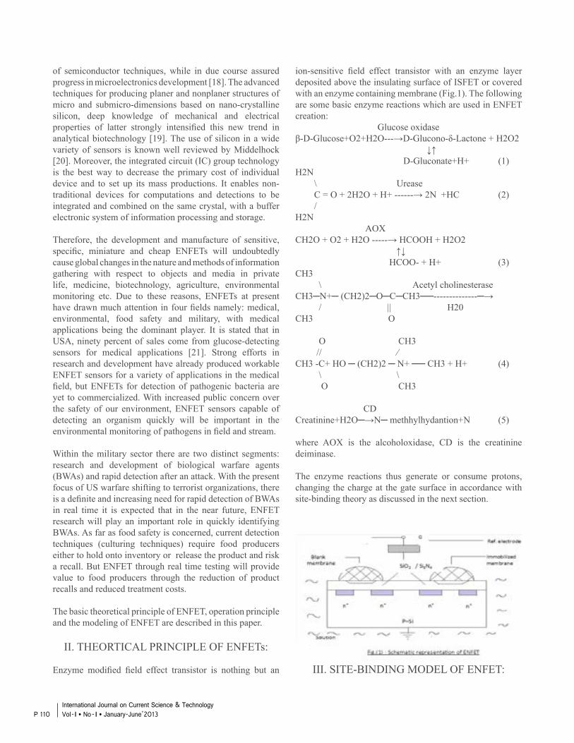
ion-sensitive field effect transistor with an enzyme layer deposited above the insulating surface of ISFET or covered with an enzyme containing membrane (Fig.1). The following are some basic enzyme reactions which are used in ENFET creation: Glucose oxidaseβ-D-Glucose+O2+H2O---→D-Glucono-δ-Lactone + H2O2 ↓↑ D-Gluconate+H+ (1)H2N \ Urease C = O + 2H2O + H+ ------→ 2N +HC (2) /H2N AOXCH2O + O2 + H2O -----→ HCOOH + H2O2 ↑↓ HCOO- + H+ (3)CH3 \ Acetyl cholinesteraseCH3N+ (CH2)2OCCH3--------------→ / || H20CH3 O O CH3 // ∕ CH3 -C+ HO (CH2)2 N+ CH3 + H+ (4) \ \ O CH3
CDCreatinine+H2O→N methhylhydantion+N (5) where AOX is the alcoholoxidase, CD is the creatinine deiminase.
The enzyme reactions thus generate or consume protons, changing the charge at the gate surface in accordance with site-binding theory as discussed in the next section.
III. SITE-BINDING MODEL OF ENFET:
of semiconductor techniques, while in due course assured progress in microelectronics development [18]. The advanced techniques for producing planer and nonplaner structures of micro and submicro-dimensions based on nano-crystalline silicon, deep knowledge of mechanical and electrical properties of latter strongly intensified this new trend in analytical biotechnology [19]. The use of silicon in a wide variety of sensors is known well reviewed by Middelhock [20]. Moreover, the integrated circuit (IC) group technology is the best way to decrease the primary cost of individual device and to set up its mass productions. It enables non-traditional devices for computations and detections to be integrated and combined on the same crystal, with a buffer electronic system of information processing and storage.
Therefore, the development and manufacture of sensitive, specific, miniature and cheap ENFETs will undoubtedly cause global changes in the nature and methods of information gathering with respect to objects and media in private life, medicine, biotechnology, agriculture, environmental monitoring etc. Due to these reasons, ENFETs at present have drawn much attention in four fields namely: medical, environmental, food safety and military, with medical applications being the dominant player. It is stated that in USA, ninety percent of sales come from glucose-detecting sensors for medical applications [21]. Strong efforts in research and development have already produced workable ENFET sensors for a variety of applications in the medical field, but ENFETs for detection of pathogenic bacteria are yet to commercialized. With increased public concern over the safety of our environment, ENFET sensors capable of detecting an organism quickly will be important in the environmental monitoring of pathogens in field and stream.
Within the military sector there are two distinct segments: research and development of biological warfare agents (BWAs) and rapid detection after an attack. With the present focus of US warfare shifting to terrorist organizations, there is a definite and increasing need for rapid detection of BWAs in real time it is expected that in the near future, ENFET research will play an important role in quickly identifying BWAs. As far as food safety is concerned, current detection techniques (culturing techniques) require food producers either to hold onto inventory or release the product and risk a recall. But ENFET through real time testing will provide value to food producers through the reduction of product recalls and reduced treatment costs.
The basic theoretical principle of ENFET, operation principle and the modeling of ENFET are described in this paper.
II. THEORTICAL PRINCIPLE OF ENFETs:
Enzyme modified field effect transistor is nothing but an
P 110International Journal on Current Science & Technology Vol - I l No- I l January-June’2013
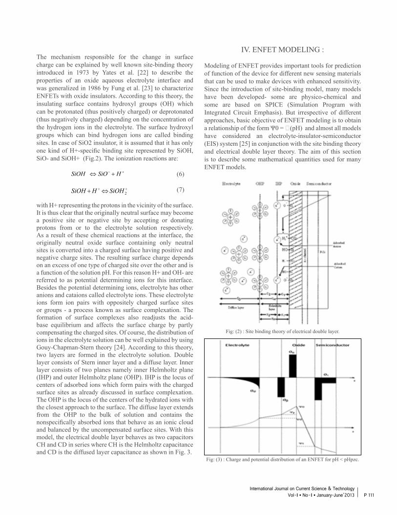
The mechanism responsible for the change in surface charge can be explained by well known site-binding theory introduced in 1973 by Yates et al. [22] to describe the properties of an oxide aqueous electrolyte interface and was generalized in 1986 by Fung et al. [23] to characterize ENFETs with oxide insulators. According to this theory, the insulating surface contains hydroxyl groups (OH) which can be protonated (thus positively charged) or deprotonated (thus negatively charged) depending on the concentration of the hydrogen ions in the electrolyte. The surface hydroxyl groups which can bind hydrogen ions are called binding sites. In case of SiO2 insulator, it is assumed that it has only one kind of H+-specific binding site represented by SiOH, SiO- and SiOH+ (Fig.2). The ionization reactions are: (6)
(7)
with H+ representing the protons in the vicinity of the surface. It is thus clear that the originally neutral surface may become a positive site or negative site by accepting or donating protons from or to the electrolyte solution respectively. As a result of these chemical reactions at the interface, the originally neutral oxide surface containing only neutral sites is converted into a charged surface having positive and negative charge sites. The resulting surface charge depends on an excess of one type of charged site over the other and is a function of the solution pH. For this reason H+ and OH- are referred to as potential determining ions for this interface. Besides the potential determining ions, electrolyte has other anions and cataions called electrolyte ions. These electrolyte ions form ion pairs with oppositely charged surface sites or groups - a process known as surface complexation. The formation of surface complexes also readjusts the acid-base equilibrium and affects the surface charge by partly compensating the charged sites. Of course, the distribution of ions in the electrolyte solution can be well explained by using Gouy-Chapman-Stern theory [24]. According to this theory, two layers are formed in the electrolyte solution. Double layer consists of Stern inner layer and a diffuse layer. Inner layer consists of two planes namely inner Helmholtz plane (IHP) and outer Helmholtz plane (OHP). IHP is the locus of centers of adsorbed ions which form pairs with the charged surface sites as already discussed in surface complexation. The OHP is the locus of the centers of the hydrated ions with the closest approach to the surface. The diffuse layer extends from the OHP to the bulk of solution and contains the nonspecifically absorbed ions that behave as an ionic cloud and balanced by the uncompensated surface sites. With this model, the electrical double layer behaves as two capacitors CH and CD in series where CH is the Helmholtz capacitance and CD is the diffused layer capacitance as shown in Fig. 3.
IV. ENFET MODELING :
Modeling of ENFET provides important tools for prediction of function of the device for different new sensing materials that can be used to make devices with enhanced sensitivity. Since the introduction of site-binding model, many models have been developed- some are physico-chemical and some are based on SPICE (Simulation Program with Integrated Circuit Emphasis). But irrespective of different approaches, basic objective of ENFET modeling is to obtain a relationship of the form Ψ0 = (pH) and almost all models have considered an electrolyte-insulator-semiconductor (EIS) system [25] in conjunction with the site binding theory and electrical double layer theory. The aim of this section is to describe some mathematical quantities used for many ENFET models.
Fig: (2) : Site binding theory of electrical double layer.
Fig: (3) : Charge and potential distribution of an ENFET for pH < pHpzc.
+− +⇔ HSiOSiOH
++ ⇔+ 2SiOHHSiOH
P 111International Journal on Current Science & Technology
Vol - I l No- I l January-June’2013
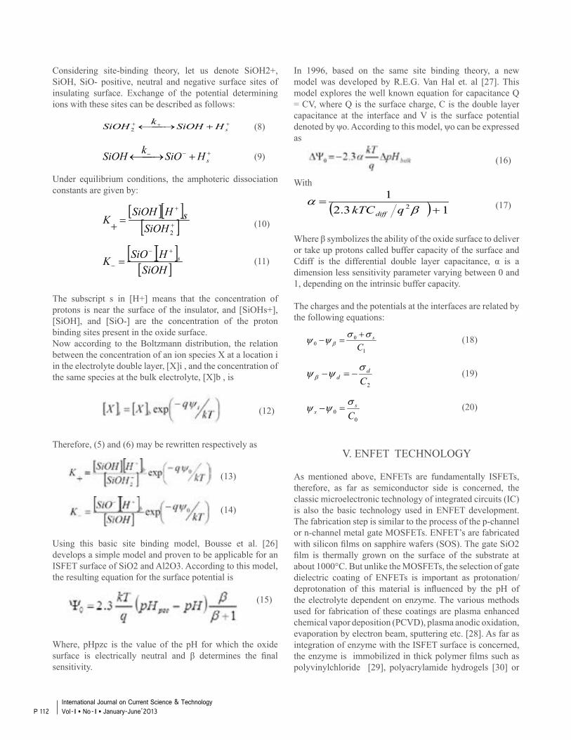
Considering site-binding theory, let us denote SiOH2+, SiOH, SiO- positive, neutral and negative surface sites of insulating surface. Exchange of the potential determining ions with these sites can be described as follows:
(8)
(9)
Under equilibrium conditions, the amphoteric dissociation constants are given by:
(10)
(11)
The subscript s in [H+] means that the concentration of protons is near the surface of the insulator, and [SiOHs+], [SiOH], and [SiO-] are the concentration of the proton binding sites present in the oxide surface.Now according to the Boltzmann distribution, the relation between the concentration of an ion species X at a location i in the electrolyte double layer, [X]i , and the concentration of the same species at the bulk electrolyte, [X]b , is
(12)
Therefore, (5) and (6) may be rewritten respectively as
(13)
(14)
Using this basic site binding model, Bousse et al. [26] develops a simple model and proven to be applicable for an ISFET surface of SiO2 and Al2O3. According to this model, the resulting equation for the surface potential is
(15)
Where, pHpzc is the value of the pH for which the oxide surface is electrically neutral and β determines the final sensitivity.
In 1996, based on the same site binding theory, a new model was developed by R.E.G. Van Hal et. al [27]. This model explores the well known equation for capacitance Q = CV, where Q is the surface charge, C is the double layer capacitance at the interface and V is the surface potential denoted by ψo. According to this model, ψo can be expressed as
(16)
With
(17)
Where β symbolizes the ability of the oxide surface to deliver or take up protons called buffer capacity of the surface and Cdiff is the differential double layer capacitance, α is a dimension less sensitivity parameter varying between 0 and 1, depending on the intrinsic buffer capacity.
The charges and the potentials at the interfaces are related by the following equations:
(18)
(19)
(20)
V. ENFET TECHNOLOGY
As mentioned above, ENFETs are fundamentally ISFETs, therefore, as far as semiconductor side is concerned, the classic microelectronic technology of integrated circuits (IC) is also the basic technology used in ENFET development. The fabrication step is similar to the process of the p-channel or n-channel metal gate MOSFETs. ENFET’s are fabricated with silicon films on sapphire wafers (SOS). The gate SiO2 film is thermally grown on the surface of the substrate at about 1000°C. But unlike the MOSFETs, the selection of gate dielectric coating of ENFETs is important as protonation/deprotonation of this material is influenced by the pH of the electrolyte dependent on enzyme. The various methods used for fabrication of these coatings are plasma enhanced chemical vapor deposition (PCVD), plasma anodic oxidation, evaporation by electron beam, sputtering etc. [28]. As far as integration of enzyme with the ISFET surface is concerned, the enzyme is immobilized in thick polymer films such as polyvinylchloride [29], polyacrylamide hydrogels [30] or
+++ +→← sHSiOHkSiOH 2
+−− +→← sHSiOkSiOH
[ ][ ][ ]+
+
=+2SiOH
sHSiOHK
[ ][ ][ ]SiOH
HSiOK s+−
− =
( ) 13.21
2 +=
βα
qkTCdiff
1
00 C
sσσψψ β+
=−
2Cd
dσψψ β −=−
00 C
ss
σψψ =−
P 112International Journal on Current Science & Technology Vol - I l No- I l January-June’2013
polyurethane [31]-[32] on ISFET device or the construction of membrane e.g. Nafion or polyvinylpyridine [33]-[35] covered crosslinked enzyme matrices on the ISFET, yield active ENFET sensing devices. Such systems however, suffer from basic limitations associated with diffusion barriers of the substrates through the polymer membranes, leading to slow response times and moderate sensitivities. It is now reported that the organization of monolayer/ multilayer enzyme- based ISFET could substantially improve the response-time and analytical performance of the ENFET device.
VI. CONCLUSION
ENFETs are microelectronic/nanoelectronic devices and have been found to be growing interest in the rapidly developing field of bioelectronics encompassing a very wide spectrum of applications. Extensive research is being carried out in a number of Universities/laboratories across the globe to develop various ENFET bioelectronic devices mainly for biomedical, bio-analytical, food processing, defense applications. Though, a series of reliable and promising results have been obtained, no successful commercial version of ENFET based biosensor is available so far. It is because the practical application of ENFET sensors is complicated by the fact that their response is affected by the pH of the medium, buffer capacity, concentration of the substrate and in some cases, e.g. for glucose, by the concentration of the co-substrate, i.e. oxygen, the buffer capacity of the solution tested depends on pH, therefore the pH change in the matrix with the immobilized enzyme depends on the initial pH. Still more essential is the pH effect on the enzyme kinetics. It is expected that through effective research activities, like the ISFET based pH sensor, the ENFET bioelectronic sensors will also be commercialized in near future.
VII. REFERENCES
[1] P.Bergveld,Development of an ion-sensitive solid- state device for neurophysiological measurements, IEEE Trans. Biomed. Eng. BME-17 (1970) 70-71.
[2] P. Bergveld, Development of an ion-sensitive solid- state device for neurophysiological measurements, IEEE Trans. Biomed. Eng. BME-17 (1970) 70-71.
[3] T. Matsuo, K.D. Wise, An integrated field effect electrode for biopotential recording, IEEE Trans. Biomed. Eng. BME-21 (1974) 485-487.
[4] P. Bergveld, Thirty years of ISFETOLOGY what happened in the past thirty years and what may happen in the next thirty years, Sensors and Actuators B, 88 (2003),1-20.
[5] Vianello F, Stefani A, dipaolo ML, Rigo A, Lui A, Margesin B,et al. Potentiometric detection of formaldehyde in air by an aldehyde dehydrogenase FET. Sensors and Actuators, B 1996;37:49-54.
[6] Senillou A, Jaffrezic-Renault N, Martelet C, Cosnier S, Aminiaturized urea sensor based on the integration of both ammonium based urea ENFET and a reference FET in a single chip. Talanta 1999; 50(1):219-26.
[7] Kharitonov AB, Zayats M, Lichtenstein A, Katz E, Willner I, Enzyme monolayer-functionalized field- effect transistors for biosensor applications. Sensors and Actuators, B 2000; 70:222-231
[8] Park K, Choi S, Lee M, Sohn B. ISFET glucose sensor system with fast recovery characteristics by employing electrolysis. Sensors and Actuators, B 2002; 83 (1-3): 90-97
[9] Dzyadevych S V, Korpan YI, Arkhipova VN Alesina MY, et al. Application of enzyme field effect transistors for determination of glucose concentrations in blood serum. Biosensors and bioelectronics, 1999;14:183-187
[10] Sergei V. dzyadevych, Alexey P. Soldatkin, yaroslav I. Korpan, Valentyna N. Arkhypova, Anna V. EI’skaya et al., Biosensors based on enzyme field -effect transistors for determination of some substrates and inhibitors. Anal Bioanal Chem, 2003, 377:496-506
[11] Starodub VM and Starodub NF, Electrochemical immune sensors based on the ion-sensitive field effect transistor for the development of the level of myoglobin. The 13th European Conference on Solid- State Transducers, September 12-15,1999
[12] D. Landheer, G. Aers, W.R Mckinnon, M.J.Deen, J.C. Ranuarez, Model for the field effect from layers of biological macromolecules on the gates of metal- oxide-semiconductor transistors. Journal of applied physics 98, 044701 (2005)
[13] J. Janata, S.D. Moss, Biomed. Eng. 6 (1976) 17.
[14] S. Caras, J. Janata, Anal. Chem. 52 (1980) 1935.
[15] Y. Miyahara, F. Matsu, T. Moriizumi, H.Matsuoka, I. Karube, S. Suzuki, Anal. Chem. Symposia Ser. 17 (1983) 501.
[16] Y. Hanazato, S. Shiono, Anal. Chem. Symposia Ser. 17 (1983) 513.
[17] P. Bergveld. Sens. Actuators B 88 (2003) 1. (P. Bergveld, Thirty years of ISFETOLOGY what happened in the past thirty years and what may happen in the next thirty years, Sensors and Actuators B, 88 (2003),1-20.)
[18] S.V. Dzyadevych et al. / Analytica Chemica Acta 568 (2006) 248-258.(S.V.Dzyadvych et al. “Enzyme biosensors based on ion-selective field effect
P 113International Journal on Current Science & Technology
Vol - I l No- I l January-June’2013
transistors” Analytica Chemica Acta 568 (2006) 248-258)
[19] K.E. Peterson. Proc. IEEE 70 (1982) 420.
[20] S.Midddelhock, Sens. Actuators A 82 (2000) 2.
[21] Evangelyn C. Alocilja, Stephen M. Radke “Market analysis of biosensor for food safety’’ Biosensors and Bioelectronics 18 (2003) 841-846.
[22] D.E.Yates, S.Levine and T.W.Healy, Site binding model of the electrical double layer at the oxide/water interface. J.Chem.Soc. Faraday Trans.,(70): 1807- 1819, 1974.
[23] C.D.Fung, P.W.Cheung and W.H.Ko, A generalized theory of an electrolyte-insulator-semiconductor field effect transistor. IEEE, ED-33(1) (1986) 8.
[24] Bard AJ, Faulkner LR., Electrochemical methods, fundamentals and applications. New York: Wiley; 1980
[25] J.C.Dutta, S. Sharma, Ion Sensitive Field Effect Transistors (ISFETs): Transducers for Biosensors. IE(I) Journal-ET,Vol.88,July 2007
[26] L. Bousse, N.F.de Rooij, P.Bergveld, “Operation of Chemically sensitive field effect sensors as a function of the properties of the insulator/ electrolyte interface, IEEE Trans. Electron Devices ED-30 (1983) 1263-1270
[27] R.E.G. Van Hal et al., “A general model to describe the electrostatic potential at electrolyte/oxide interfaces, Adv.Coll. Interf. Science, 69 (1996) 31-62
[28] Tatsuo Akiyama, Yusuke Ujihira, Yoichi Okabe, Takuo Sugano and Eiji niki “Ion- Sensitive Field-Effect Transistors with Inorganic gate Oxide for pH Sensing” IEEE Trans. On Electron Devices, Vol, ED-29, No.12, December 1982, p.1936-1941.
[29] A. Senillou, N. Jaffrezic-Renault, C. Martelet, S.Cosnier, A miniaturized urea enzyme field effect transistor and a reference field effect transistor in a
single chip, Talanto 50 (1999) 219-226.
[30] C.Jimenez, J. Bartroli, N.F. de Rooij, M. Koudelka- Hep. Use of Photopolymerizable membranes basedd on polycrylamide hydrogels for enzymatic microsensor construction, Anal. Chim. Acta 351 (1997) 169- 176.
[31] C. Puig-Lleixa,C Jimenez, J. Alonso, J. Bartroli, polyurethane-acrylate photocurable polymeric membrane for ion- sensitive field-effect transistor- based urea biosensors, anal. Chim. Acta 389 (1999) 179-188.
[32] J.Munoz, C. Jimenez, A. Bratov, J. Bartroli, S. Alegret, C. Dominguez, Photosensitive polyurethanes applied to the development of CHEMFET and ENFET devices for biomedical sensing, Biosens. Bioelectron. 12 (1997) 577-585.
[33] D.V. Gorchkov, A.P. Soldatkin, S. Poyard, N. Jaffrezic-Renault, C. Martelet, Application of charged polymeric materials as additional permselective membranes for improvement of the performance characteristics of urea-sensitive enzymatic field effect transistors : 1.Determination of urea in model solutions, Mater. Sci. Eng., C 5 (1997) 23-28.
[34] D.V. Gorchkov, S. Poyard, A.P. Soldatkin, N. Jaffrezic-Renault, C. Martelet, Application of charged polymeric materials as additional permselective membranes for improvement of the performance characteristics of urea-sensitive ENFETs : 2.Urea determination in blood serum, Mater. Sci. Eng., C 5 (1997) 29-34.
[35] A.P. Soldatkin, D.V. Gorchkov, C. Martelet ,N. Jaffrezic-Renault, Application of charged polymeric materials as additional permselective membranes for modulation of the working characteristics of penicillin sensitive ENFETs, Mater. Sci. Eng., C 5 (1997) 35-40.
P 114International Journal on Current Science & Technology Vol - I l No- I l January-June’2013
ACETYLCHOLINE GATED SPIKING NEURON MODEL
Soumik Roy1, Meenakshi Boro2 , Jiten Ch Dutta3, Reginald H. Vanlalchaka4
Bioelectronics Division, Dept of ECE, Tezpur UniversityNapaam Post, Tezpur, Assam - 784 028, India
[email protected], [email protected] [email protected], [email protected]
ABSTRACT
The ion channels of post synaptic neuron shows variable conductance which depends on the transmitters diffused through the synaptic cleft and binding with the receptor sites. The binding with the receptor site is enzyme based and so the enzyme acetylcholine is considered for excitatory state of the neuron. The activity of binding can be represented by enzyme modified field effect transistor (ENFET) sensitive to acetylcholine. Acetylcholine sensitive ENFET functions not only as a voltage controlled conductance but can also provide a means of measurement of specific neurotransmitters that bind with the receptor sites of postsynaptic membrane. The ENFET is used as the circuit analogue to simulate a group of excitatory transmitter-gated ion channels. This analogue is incorporated into a circuit model of the postsynaptic membrane at the neuromuscular junction to substitute the variable Na+ conductance. Simulation is performed in MATLAB for normal excitatory state and the results are presented.
Keywords : Ion channels, Post synaptic neuron, Synaptic cleft, Acetylcholine, ENFET.
I. NTRODUCTION
Communication in the nervous system occurs biochemically at the synapse. The synapse consists of a presynaptic neuron, synaptic cleft and postsynaptic neuron. Neurotransmitter, such as acetylcholine is released by the presynaptic terminals into the synaptic cleft. The transmitter diffuses and binds with specific receptors in the postsynaptic cell. The binding initiates the opening of transmitter-gated ion channels, and subsequent influx of ions into the cell. The postsynaptic membrane of a single neuron can have excitatory and inhibitory transmitter-gated ion channels. Generally, excitatory channels are specific to sodium ions and inhibitory channels are specific to chloride ions. The excitatory and inhibitory ionic current control the change in membrane potential.
The influx of sodium ions causes an excitatory post synaptic membrane potential (EPSP), whereas the influx of chloride ions causes an inhibitory postsynaptic membrane potential (IPSP). When excitation predominates the membrane potential increases. If a sufficient number of transmitter gated sodium channels are open, then the membrane potential exceeds the threshold for initiating an action potential. The acetylcholine - receptor binding activity initiates the opening of sodium channels causing the flow of sodium ions into the cell. If a sufficient number of channels open, then the membrane potential exceeds the threshold for initiating an action potential[1].When inhibition predominates the membrane potential decreases (or hyperpolarizes), and triggering of an action potential is impeded. Neurons are very dynamic objects. Some types of neurons called pacemakers are capable of spontaneously firing in a rhythmic fashion, others can fire randomly. These behaviours are caused by very complex and highly dynamic properties within the neurons. Because of their intrinsic complexity, models are usually difficult to analyze and are computationally expensive in numerical implementations. For this reason, simple phenomenological spiking neuron models such as integrate-and-fire (IF) models [2]-[3] are highly popular and have been used to discuss aspects of neural coding, memory, or network dynamics [4] -[5]. Model neurons which include time are those in which the actual timing of the input matters. Models of this form can be sensitive to the actual timing of their inputs. The simplest form of spiking neural model which includes time, gives their output in the form of spikes. Thus the output can be characterised by
(1)
Where is the time of the ’th spike train in a train of ‘ ’ spikes [6].
Neuron models are proposed by neuroscientist to simulate neurons [7]-[8] for explaining the active principle associated with it. Among these models, neuroscientists have, utilized the Hodgkin-Huxley (H-H) model as a circuit analogue of the axonal membrane.
The H-H equations are simple and elegant tool, capable of
1( : 1... ),i i iS t i n t t += = <
P 115International Journal on Current Science & Technology
Vol - I l No- I l January-June’2013
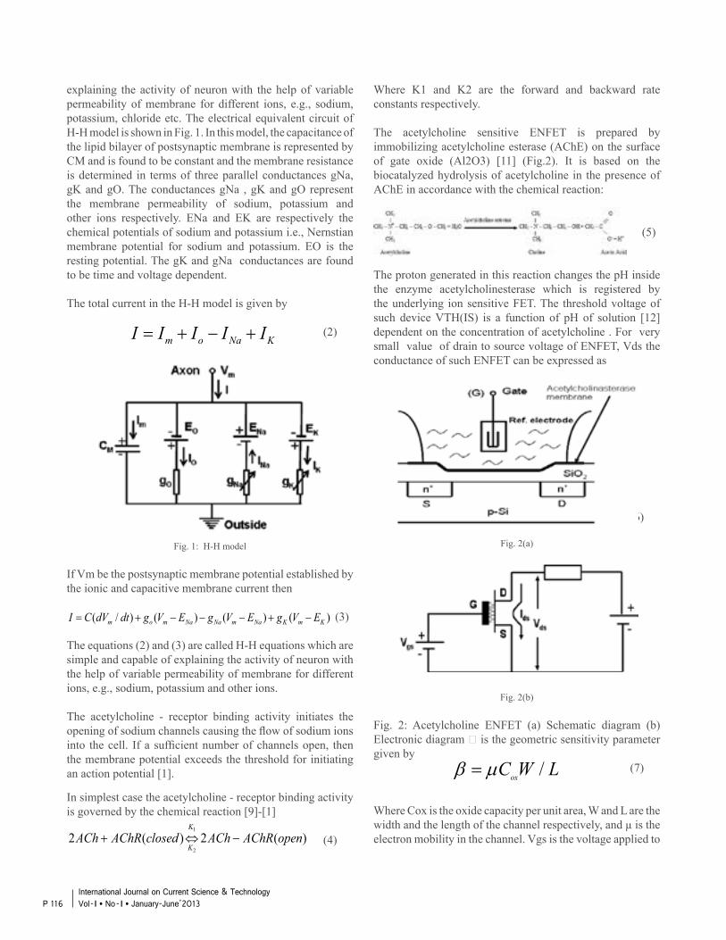
explaining the activity of neuron with the help of variable permeability of membrane for different ions, e.g., sodium, potassium, chloride etc. The electrical equivalent circuit of H-H model is shown in Fig. 1. In this model, the capacitance of the lipid bilayer of postsynaptic membrane is represented by CM and is found to be constant and the membrane resistance is determined in terms of three parallel conductances gNa, gK and gO. The conductances gNa , gK and gO represent the membrane permeability of sodium, potassium and other ions respectively. ENa and EK are respectively the chemical potentials of sodium and potassium i.e., Nernstian membrane potential for sodium and potassium. EO is the resting potential. The gK and gNa conductances are found to be time and voltage dependent.
The total current in the H-H model is given by
(2)
Fig. 1: H-H model
If Vm be the postsynaptic membrane potential established by the ionic and capacitive membrane current then
(3)
The equations (2) and (3) are called H-H equations which are simple and capable of explaining the activity of neuron with the help of variable permeability of membrane for different ions, e.g., sodium, potassium and other ions.
The acetylcholine - receptor binding activity initiates the opening of sodium channels causing the flow of sodium ions into the cell. If a sufficient number of channels open, then the membrane potential exceeds the threshold for initiating an action potential [1].
In simplest case the acetylcholine - receptor binding activity is governed by the chemical reaction [9]-[1]
(4)
Where K1 and K2 are the forward and backward rate constants respectively.
The acetylcholine sensitive ENFET is prepared by immobilizing acetylcholine esterase (AChE) on the surface of gate oxide (Al2O3) [11] (Fig.2). It is based on the biocatalyzed hydrolysis of acetylcholine in the presence of AChE in accordance with the chemical reaction:
(5)
The proton generated in this reaction changes the pH inside the enzyme acetylcholinesterase which is registered by the underlying ion sensitive FET. The threshold voltage of such device VTH(IS) is a function of pH of solution [12] dependent on the concentration of acetylcholine . For very small value of drain to source voltage of ENFET, Vds the conductance of such ENFET can be expressed as
(6)
Fig. 2(a)
Fig. 2(b)
Fig. 2: Acetylcholine ENFET (a) Schematic diagram (b) Electronic diagram is the geometric sensitivity parameter given by (7)
Where Cox is the oxide capacity per unit area, W and L are the width and the length of the channel respectively, and µ is the electron mobility in the channel. Vgs is the voltage applied to
m o Na KI I I I I= + − +
( / ) ( ) ( ) ( )m o m Na Na m Na K m KI C dV dt g V E g V E g V E= + − − − + −
1
2
2 ( ) 2 ( )K
KACh AChR closed ACh AChR open+ ⇔ −
/oxC W Lβ µ=
P 116International Journal on Current Science & Technology Vol - I l No- I l January-June’2013
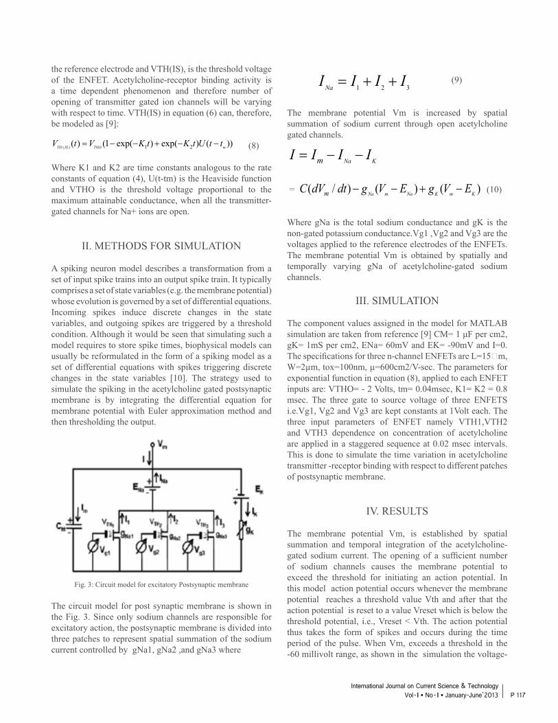
the reference electrode and VTH(IS), is the threshold voltage of the ENFET. Acetylcholine-receptor binding activity is a time dependent phenomenon and therefore number of opening of transmitter gated ion channels will be varying with respect to time. VTH(IS) in equation (6) can, therefore, be modeled as [9]:
(8)
Where K1 and K2 are time constants analogous to the rate constants of equation (4), U(t-tm) is the Heaviside function and VTHO is the threshold voltage proportional to the maximum attainable conductance, when all the transmitter-gated channels for Na+ ions are open.
II. METHODS FOR SIMULATION
A spiking neuron model describes a transformation from a set of input spike trains into an output spike train. It typically comprises a set of state variables (e.g. the membrane potential) whose evolution is governed by a set of differential equations. Incoming spikes induce discrete changes in the state variables, and outgoing spikes are triggered by a threshold condition. Although it would be seen that simulating such a model requires to store spike times, biophysical models can usually be reformulated in the form of a spiking model as a set of differential equations with spikes triggering discrete changes in the state variables [10]. The strategy used to simulate the spiking in the acetylcholine gated postsynaptic membrane is by integrating the differential equation for membrane potential with Euler approximation method and then thresholding the output.
Fig. 3: Circuit model for excitatory Postsynaptic membrane
The circuit model for post synaptic membrane is shown in the Fig. 3. Since only sodium channels are responsible for excitatory action, the postsynaptic membrane is divided into three patches to represent spatial summation of the sodium current controlled by gNa1, gNa2 ,and gNa3 where
(9)
The membrane potential Vm is increased by spatial summation of sodium current through open acetylcholine gated channels.
= (10)
Where gNa is the total sodium conductance and gK is the non-gated potassium conductance.Vg1 ,Vg2 and Vg3 are the voltages applied to the reference electrodes of the ENFETs. The membrane potential Vm is obtained by spatially and temporally varying gNa of acetylcholine-gated sodium channels.
III. SIMULATION
The component values assigned in the model for MATLAB simulation are taken from reference [9] CM= 1 μF per cm2, gK= 1mS per cm2, ENa= 60mV and EK= -90mV and I=0. The specifications for three n-channel ENFETs are L=15m, W=2µm, tox=100nm, µ=600cm2/V-sec. The parameters for exponential function in equation (8), applied to each ENFET inputs are: VTHO= - 2 Volts, tm= 0.04msec, K1= K2 = 0.8 msec. The three gate to source voltage of three ENFETS i.e.Vg1, Vg2 and Vg3 are kept constants at 1Volt each. The three input parameters of ENFET namely VTH1,VTH2 and VTH3 dependence on concentration of acetylcholine are applied in a staggered sequence at 0.02 msec intervals. This is done to simulate the time variation in acetylcholine transmitter -receptor binding with respect to different patches of postsynaptic membrane.
IV. RESULTS
The membrane potential Vm, is established by spatial summation and temporal integration of the acetylcholine-gated sodium current. The opening of a sufficient number of sodium channels causes the membrane potential to exceed the threshold for initiating an action potential. In this model action potential occurs whenever the membrane potential reaches a threshold value Vth and after that the action potential is reset to a value Vreset which is below the threshold potential, i.e., Vreset < Vth. The action potential thus takes the form of spikes and occurs during the time period of the pulse. When Vm, exceeds a threshold in the -60 millivolt range, as shown in the simulation the voltage-
( ) 1 2( ) (1 exp( ) exp( ) ( ))TH IS THO mV t V K t K t U t t= − − + − −
1 2 3NaI I I I= + +
Na KmI I I I= − −
( / ) ( ) ( )Na m Na K m KmC dV dt g V E g V E− − + −
P 117International Journal on Current Science & Technology
Vol - I l No- I l January-June’2013
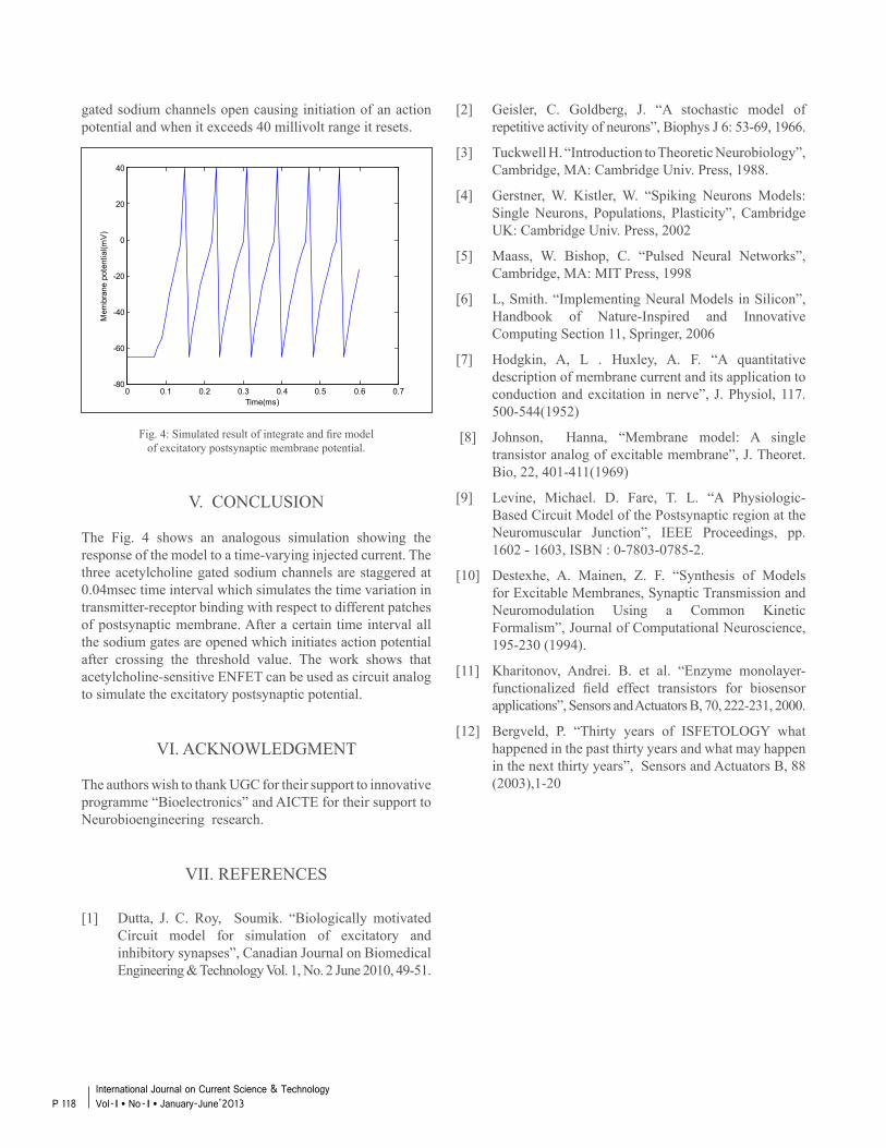
gated sodium channels open causing initiation of an action potential and when it exceeds 40 millivolt range it resets.
Fig. 4: Simulated result of integrate and fire modelof excitatory postsynaptic membrane potential.
V. CONCLUSION
The Fig. 4 shows an analogous simulation showing the response of the model to a time-varying injected current. The three acetylcholine gated sodium channels are staggered at 0.04msec time interval which simulates the time variation in transmitter-receptor binding with respect to different patches of postsynaptic membrane. After a certain time interval all the sodium gates are opened which initiates action potential after crossing the threshold value. The work shows that acetylcholine-sensitive ENFET can be used as circuit analog to simulate the excitatory postsynaptic potential.
VI. ACKNOWLEDGMENT
The authors wish to thank UGC for their support to innovative programme “Bioelectronics” and AICTE for their support to Neurobioengineering research.
VII. REFERENCES
[1] Dutta, J. C. Roy, Soumik. “Biologically motivated Circuit model for simulation of excitatory and inhibitory synapses”, Canadian Journal on Biomedical Engineering & Technology Vol. 1, No. 2 June 2010, 49-51.
[2] Geisler, C. Goldberg, J. “A stochastic model of repetitive activity of neurons”, Biophys J 6: 53-69, 1966.
[3] Tuckwell H. “Introduction to Theoretic Neurobiology”, Cambridge, MA: Cambridge Univ. Press, 1988.
[4] Gerstner, W. Kistler, W. “Spiking Neurons Models: Single Neurons, Populations, Plasticity”, Cambridge UK: Cambridge Univ. Press, 2002
[5] Maass, W. Bishop, C. “Pulsed Neural Networks”, Cambridge, MA: MIT Press, 1998
[6] L, Smith. “Implementing Neural Models in Silicon”, Handbook of Nature-Inspired and Innovative Computing Section 11, Springer, 2006
[7] Hodgkin, A, L . Huxley, A. F. “A quantitative description of membrane current and its application to conduction and excitation in nerve”, J. Physiol, 117. 500-544(1952)
[8] Johnson, Hanna, “Membrane model: A single transistor analog of excitable membrane”, J. Theoret. Bio, 22, 401-411(1969)
[9] Levine, Michael. D. Fare, T. L. “A Physiologic- Based Circuit Model of the Postsynaptic region at the Neuromuscular Junction”, IEEE Proceedings, pp. 1602 - 1603, ISBN : 0-7803-0785-2.
[10] Destexhe, A. Mainen, Z. F. “Synthesis of Models for Excitable Membranes, Synaptic Transmission and Neuromodulation Using a Common Kinetic Formalism”, Journal of Computational Neuroscience, 195-230 (1994).
[11] Kharitonov, Andrei. B. et al. “Enzyme monolayer- functionalized field effect transistors for biosensor applications”, Sensors and Actuators B, 70, 222-231, 2000.
[12] Bergveld, P. “Thirty years of ISFETOLOGY what happened in the past thirty years and what may happen in the next thirty years”, Sensors and Actuators B, 88 (2003),1-20
0 0.1 0.2 0.3 0.4 0.5 0.6 0.7-80
-60
-40
-20
0
20
40
Time(ms)
Mem
bran
e po
tent
ial(m
V)
P 118International Journal on Current Science & Technology Vol - I l No- I l January-June’2013
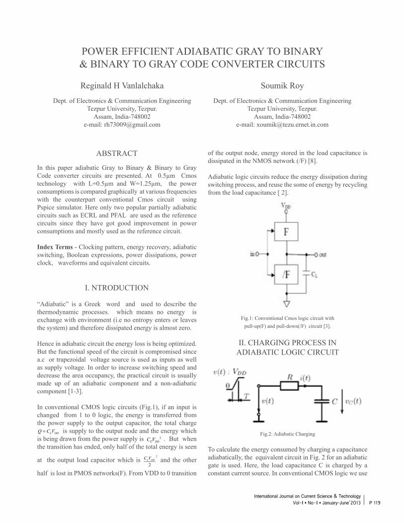
POWER EFFICIENT ADIABATIC GRAY TO BINARY& BINARY TO GRAY CODE CONVERTER CIRCUITS
Soumik Roy
Dept. of Electronics & Communication EngineeringTezpur University, Tezpur.
Assam, India-748002e-mail: [email protected]
Reginald H Vanlalchaka
Dept. of Electronics & Communication EngineeringTezpur University, Tezpur.
Assam, India-748002e-mail: [email protected]
ABSTRACT
In this paper adiabatic Gray to Binary & Binary to Gray Code converter circuits are presented. At 0.5µm Cmos technology with L=0.5µm and W=1.25µm, the power consumptions is compared graphically at various frequencies with the counterpart conventional Cmos circuit using Pspice simulator. Here only two popular partially adiabatic circuits such as ECRL and PFAL are used as the reference circuits since they have got good improvement in power consumptions and mostly used as the reference circuit.
Index Terms - Clocking pattern, energy recovery, adiabatic switching, Boolean expressions, power dissipations, power clock, waveforms and equivalent circuits.
I. NTRODUCTION
“Adiabatic” is a Greek word and used to describe the thermodynamic processes. which means no energy is exchange with environment (i.e no entropy enters or leaves the system) and therefore dissipated energy is almost zero.
Hence in adiabatic circuit the energy loss is being optimized. But the functional speed of the circuit is compromised since a.c or trapezoidal voltage source is used as inputs as well as supply voltage. In order to increase switching speed and decrease the area occupancy, the practical circuit is usually made up of an adiabatic component and a non-adiabatic component [1-3].
In conventional CMOS logic circuits (Fig.1), if an input is changed from 1 to 0 logic, the energy is transferred from the power supply to the output capacitor, the total charge is supply to the output node and the energy which is being drawn from the power supply is . . But when the transition has ended, only half of the total energy is seen
at the output load capacitor which is and the other
half is lost in PMOS networks(F). From VDD to 0 transition
of the output node, energy stored in the load capacitance is dissipated in the NMOS network (/F) [8].
Adiabatic logic circuits reduce the energy dissipation during switching process, and reuse the some of energy by recycling from the load capacitance [ 2].
Fig.1: Conventional Cmos logic circuit withpull-up(F) and pull-down(/F) circuit [3].
II. CHARGING PROCESS IN
ADIABATIC LOGIC CIRCUIT
Fig.2: Adiabatic Charging
To calculate the energy consumed by charging a capacitance adiabatically, the equivalent circuit in Fig. 2 for an adiabatic gate is used. Here, the load capacitance C is charged by a constant current source. In conventional CMOS logic we use
L DDQ C V=2
L DDC V
2
2L DDC V
P 119International Journal on Current Science & Technology
Vol - I l No- I l January-June’2013
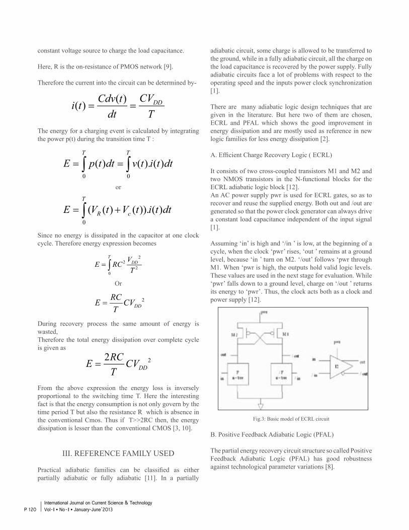
constant voltage source to charge the load capacitance.
Here, R is the on-resistance of PMOS network [9].
Therefore the current into the circuit can be determined by-
The energy for a charging event is calculated by integrating the power p(t) during the transition time T :
or
Since no energy is dissipated in the capacitor at one clock cycle. Therefore energy expression becomes
Or
During recovery process the same amount of energy is wasted,Therefore the total energy dissipation over complete cycle is given as
From the above expression the energy loss is inversely proportional to the switching time T. Here the interesting fact is that the energy consumption is not only govern by the time period T but also the resistance R which is absence in the conventional Cmos. Thus if T>>2RC then, the energy dissipation is lesser than the conventional CMOS [3, 10].
III. REFERENCE FAMILY USED
Practical adiabatic families can be classified as either partially adiabatic or fully adiabatic [11]. In a partially
adiabatic circuit, some charge is allowed to be transferred to the ground, while in a fully adiabatic circuit, all the charge on the load capacitance is recovered by the power supply. Fully adiabatic circuits face a lot of problems with respect to the operating speed and the inputs power clock synchronization [1].
There are many adiabatic logic design techniques that are given in the literature. But here two of them are chosen, ECRL and PFAL which shows the good improvement in energy dissipation and are mostly used as reference in new logic families for less energy dissipation [2].
A. Efficient Charge Recovery Logic ( ECRL)
It consists of two cross-coupled transistors M1 and M2 and two NMOS transistors in the N-functional blocks for the ECRL adiabatic logic block [12].An AC power supply pwr is used for ECRL gates, so as to recover and reuse the supplied energy. Both out and /out are generated so that the power clock generator can always drive a constant load capacitance independent of the input signal [1].
Assuming ‘in’ is high and ‘/in ’ is low, at the beginning of a cycle, when the clock ‘pwr’ rises, ‘out ’ remains at a ground level, because ‘in ’ turn on M2. ‘/out’ follows ‘pwr through M1. When ‘pwr is high, the outputs hold valid logic levels. These values are used in the next stage for evaluation. While ‘pwr’ falls down to a ground level, charge on ‘/out ’ returns its energy to ‘pwr’. Thus, the clock acts both as a clock and power supply [12].
Fig.3: Basic model of ECRL circuit
B. Positive Feedback Adiabatic Logic (PFAL)
The partial energy recovery circuit structure so called Positive Feedback Adiabatic Logic (PFAL) has good robustness against technological parameter variations [8].
( )( ) DDCVCdv ti tdt T
= =
0 0
( ) ( ). ( )T T
E p t dt v t i t dt= =∫ ∫
0
( ( ) ( )). ( )T
R cE V t V t i t dt= +∫
22
20
TDDVE RCT
= ∫
2DD
RCE CVT
=
22DD
RCE CVT
=
P 120International Journal on Current Science & Technology Vol - I l No- I l January-June’2013
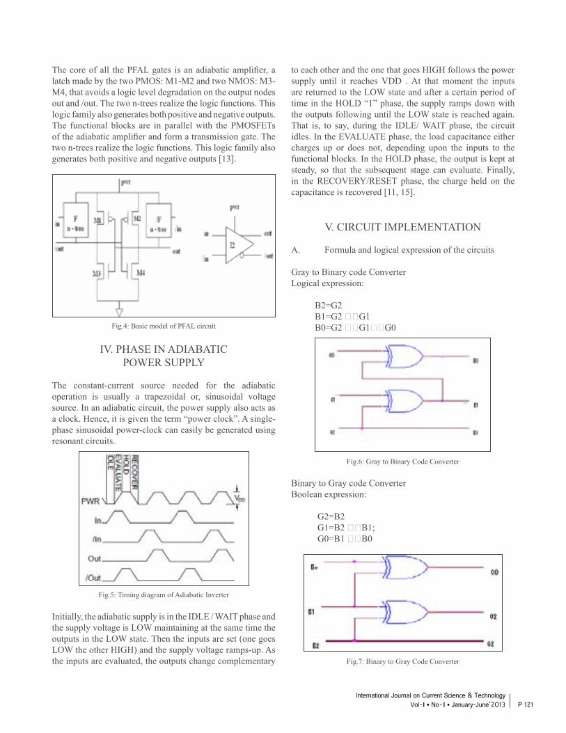
The core of all the PFAL gates is an adiabatic amplifier, a latch made by the two PMOS: M1-M2 and two NMOS: M3-M4, that avoids a logic level degradation on the output nodes out and /out. The two n-trees realize the logic functions. This logic family also generates both positive and negative outputs. The functional blocks are in parallel with the PMOSFETs of the adiabatic amplifier and form a transmission gate. The two n-trees realize the logic functions. This logic family also generates both positive and negative outputs [13].
Fig.4: Basic model of PFAL circuit
IV. PHASE IN ADIABATICPOWER SUPPLY
The constant-current source needed for the adiabatic operation is usually a trapezoidal or, sinusoidal voltage source. In an adiabatic circuit, the power supply also acts as a clock. Hence, it is given the term “power clock”. A single-phase sinusoidal power-clock can easily be generated using resonant circuits.
Fig.5: Timing diagram of Adiabatic Inverter
Initially, the adiabatic supply is in the IDLE / WAIT phase and the supply voltage is LOW maintaining at the same time the outputs in the LOW state. Then the inputs are set (one goes LOW the other HIGH) and the supply voltage ramps-up. As the inputs are evaluated, the outputs change complementary
to each other and the one that goes HIGH follows the power supply until it reaches VDD . At that moment the inputs are returned to the LOW state and after a certain period of time in the HOLD “1” phase, the supply ramps down with the outputs following until the LOW state is reached again. That is, to say, during the IDLE/ WAIT phase, the circuit idles. In the EVALUATE phase, the load capacitance either charges up or does not, depending upon the inputs to the functional blocks. In the HOLD phase, the output is kept at steady, so that the subsequent stage can evaluate. Finally, in the RECOVERY/RESET phase, the charge held on the capacitance is recovered [11, 15].
V. CIRCUIT IMPLEMENTATION
A. Formula and logical expression of the circuits
Gray to Binary code Converter Logical expression:
B2=G2B1=G2 G1B0=G2 G1G0
Fig.6: Gray to Binary Code Converter
Binary to Gray code Converter Boolean expression:
G2=B2G1=B2 B1; G0=B1 B0
Fig.7: Binary to Gray Code Converter
P 121International Journal on Current Science & Technology
Vol - I l No- I l January-June’2013
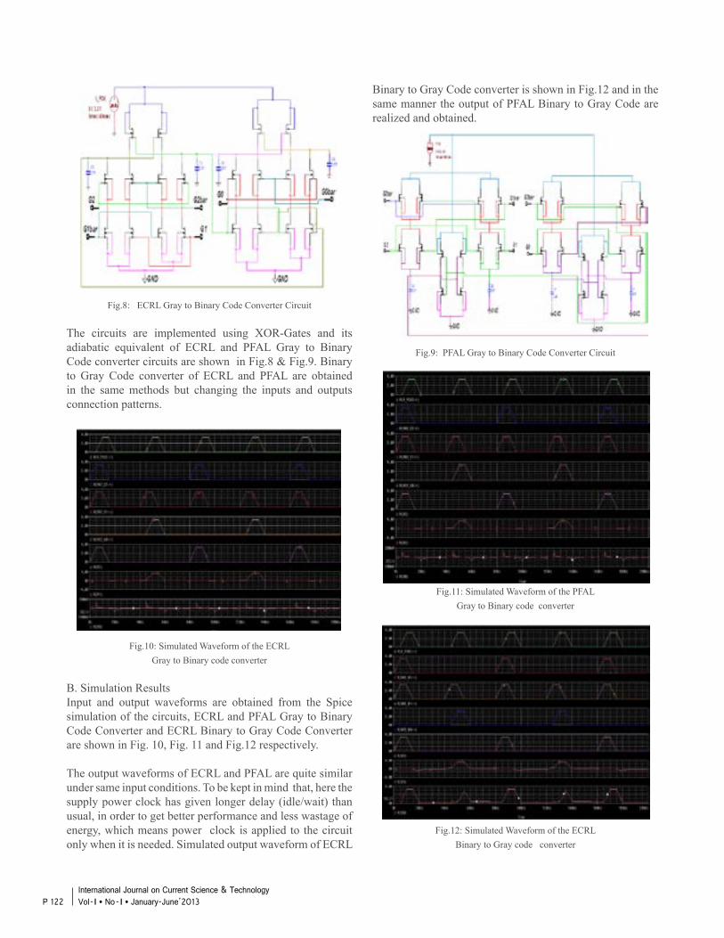
Fig.8: ECRL Gray to Binary Code Converter Circuit
The circuits are implemented using XOR-Gates and its adiabatic equivalent of ECRL and PFAL Gray to Binary Code converter circuits are shown in Fig.8 & Fig.9. Binary to Gray Code converter of ECRL and PFAL are obtained in the same methods but changing the inputs and outputs connection patterns.
Fig.10: Simulated Waveform of the ECRL Gray to Binary code converter
B. Simulation ResultsInput and output waveforms are obtained from the Spice simulation of the circuits, ECRL and PFAL Gray to Binary Code Converter and ECRL Binary to Gray Code Converter are shown in Fig. 10, Fig. 11 and Fig.12 respectively.
The output waveforms of ECRL and PFAL are quite similar under same input conditions. To be kept in mind that, here the supply power clock has given longer delay (idle/wait) than usual, in order to get better performance and less wastage of energy, which means power clock is applied to the circuit only when it is needed. Simulated output waveform of ECRL
Binary to Gray Code converter is shown in Fig.12 and in the same manner the output of PFAL Binary to Gray Code are realized and obtained.
Fig.9: PFAL Gray to Binary Code Converter Circuit
Fig.11: Simulated Waveform of the PFAL Gray to Binary code converter
Fig.12: Simulated Waveform of the ECRLBinary to Gray code converter
P 122International Journal on Current Science & Technology Vol - I l No- I l January-June’2013
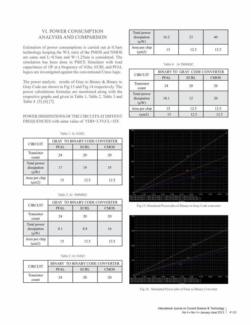
VI. POWER CONSUMPTIONANALYSIS AND COMPARISON
Estimation of power consumptions is carried out at 0.5um technology keeping the W/L ratio of the PMOS and NMOS are same and L=0.5um and W=1.25um is considered. The simulation has been done in PSICE Simulator with load capacitance of 1fF at a frequency of 1Ghz. ECRL and PFAL logics are investigated against the conventional Cmos logic.
The power analysis results of Gray to Binary & Binary to Gray Code are shown in Fig.13 and Fig.14 respectively. The power calculations formulas are mentioned along with the respective graphs and given in Table 1, Table 2, Table 3 and Table 4 [5] [6] [7].
POWER DISSIPATIONS OF THE CIRCUITS AT DIFFENT FREQUENCIES with same value of VDD=3.3V,CL=1FF.
Table 1: At 1GHZ:
CIRCUITGRAY TO BINARY CODE CONVERTER
PFAL ECRL CMOSTransistor
count 24 20 20
Total power dissipation
(µW)17 19 35
Area per chip (µm2) 15 12.5 12.5
Table 2: At 500MHZ:
CIRCUITGRAY TO BINARY CODE CONVERTER
PFAL ECRL CMOSTransistor
count 24 20 20
Total power dissipation
(µW)8.1 8.8 16
Area per chip (µm2) 15 12.5 12.5
Table 3: At 1GHZ:
CIRCUITBINARY TO BINARY CODE CONVERTER
PFAL ECRL CMOSTransistor
count 24 20 20
Total power dissipation
(µW)16.2 23 40
Area per chip (µm2) 15 12.5 12.5
Table 4: At 500MHZ:
CIRCUITBINARY TO GRAY CODE CONVERTER
PFAL ECRL CMOSTransistor
count 24 20 20
Total power dissipation
(µW)10.1 12 20
Area per chip 15 12.5 12.5 (µm2) 15 12.5 12.5
Fig.13: Simulated Power plot of Binary to Gray Code converter
Fig.14: Simulated Power plot of Gray to Binary Converter
P 121International Journal on Current Science & Technology
Vol - I l No- I l January-June’2013
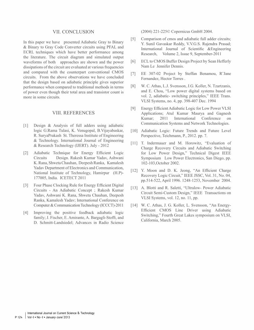
VII. CONCLUSION
In this paper we have presented Adiabatic Gray to Binary & Binary to Gray Code Converter circuits using PFAL and ECRL techniques which have better performance among the literature. The circuit diagram and simulated output waveforms of both approaches are shown and the power dissipations of the circuit are evaluated at various frequencies and compared with the counterpart conventional CMOS circuits. From the above observations we have concluded that the design based on adiabatic principle gives superior performance when compared to traditional methods in terms of power even though their total area and transistor count is more in some circuits.
VIII. REFERENCES
[1] Design & Analysis of full adders using adiabatic logic G.Rama Tulasi, K. Venugopal, B.Vijayabaskar, R. SuryaPrakash St. Theressa Institute of Engineering & Technology. International Journal of Engineering & Research Technology (IJERT). July - 2012
[2] Adiabatic Technique for Energy Efficient Logic Circuits Design. Rakesh Kumar Yadav, Ashwani K. Rana, Shweta Chauhan, Deepesh Ranka, Kamalesh Yadav Department of Electronics and Communication, National Institute of Technology, Hamirpur (H.P)- 177005, India. ICETECT 2011
[3] Four Phase Clocking Rule for Energy Efficient Digital Circuits - An Adiabatic Concept ; Rakesh Kumar Yadav, Ashwani K. Rana, Shweta Chauhan, Deepesh Ranka, Kamalesh Yadav; International Conference on Computer & Communication Technology (ICCCT)-2011
[4] Improving the positive feedback adiabatic logic family; J. Fischer, E. Amirante, A. Bargagli-Stoffi, and D. Schmitt-Landsiedel; Advances in Radio Science
(2004) 221-225© Copernicus GmbH 2004.
[5] Comparison of cmos and adiabatic full adder circuits; Y. Sunil Gavaskar Reddy, V.V.G.S. Rajendra Prasad; International Journal of Scientific &Engineering Research, Volume 2, Issue 9, September-2011
[6] ECL to CMOS Buffer Design Project by Sean Hefferly Nam Le Jennifer Dennis.
[7] EE 307-02 Project by Steffan Benamou, R’Jane Fernandez, Hector Torres .
[8] W. C. Athas, L.J. Svensson, J.G. Koller, N. Tzartzanis, and E. Chou, “Low power digital systems based on vol. 2, adiabatic- switching principles,” IEEE Trans. VLSI Systems, no. 4, pp. 398-407 Dec. 1994
[9] Energy Efficient Adiabatic Logic for Low Power VLSI Applications; Atul Kumar Maurya and Gagnesh Kumar; 2011 International Conference on Communication Systems and Network Technologies.
[10] Adiabatic Logic: Future Trends and Future Level Perspective, Teichmann, P., 2012. pp. 7.
[11] T. Indermauer and M. Horowitz, “Evaluation of Charge Recovery Circuits and Adiabatic Switching for Low Power Design,” Technical Digest IEEE Symposium Low Power Electronics, San Diego, pp. 102-103,October 2002.
[12] Y. Moon and D. K. Jeong, “An Efficient Charge Recovery Logic Circuit,” IEEE JSSC, Vol. 31, No. 04, pp.514-522, April 1996. 1248-1253, November 2004.
[13] A. Blotti and R. Saletti, “Ultralow- Power Adiabatic Circuit Semi-Custom Design,” IEEE Transactions on VLSI Systems, vol. 12, no. 11, pp.
[14] W. C. Athas, J. G. Koller, L. Svensson, “An Energy- Efficient CMOS Line Driver using Adiabatic Switching,” Fourth Great Lakes symposium on VLSI, California, March 2005.
P 124International Journal on Current Science & Technology Vol - I l No- I l January-June’2013
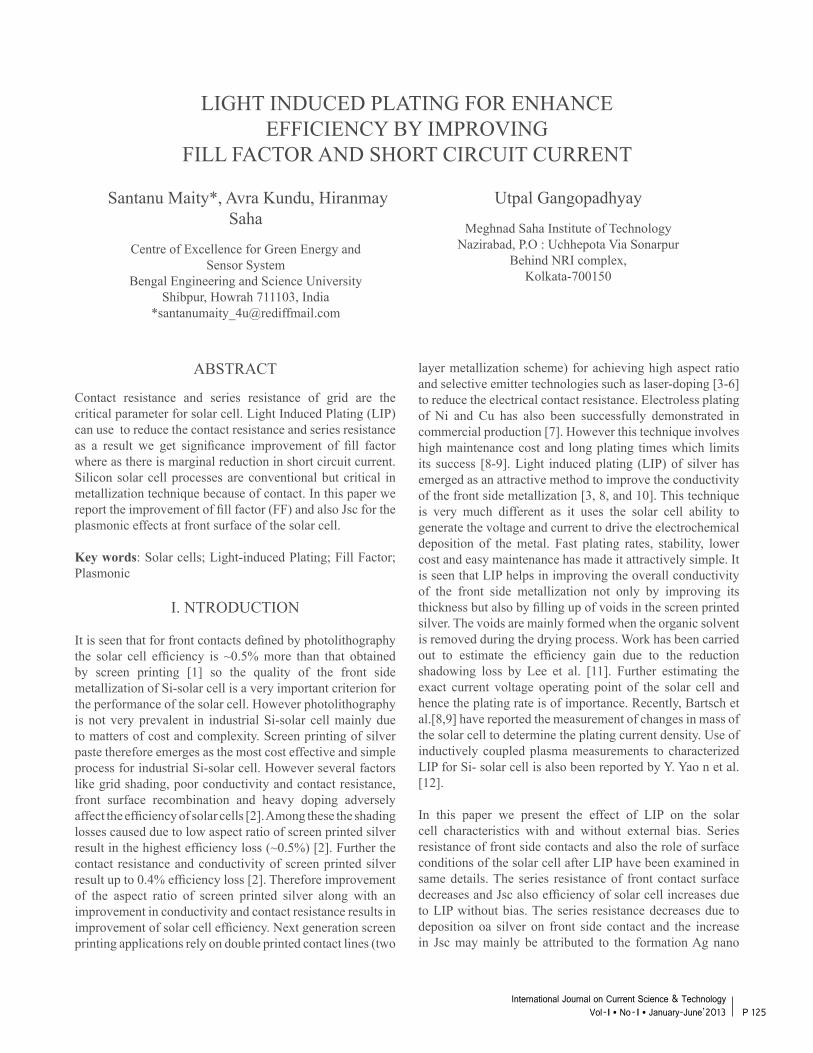
LIGHT INDUCED PLATING FOR ENHANCE EFFICIENCY BY IMPROVING
FILL FACTOR AND SHORT CIRCUIT CURRENT
Santanu Maity*, Avra Kundu, Hiranmay Saha
Centre of Excellence for Green Energy andSensor System
Bengal Engineering and Science UniversityShibpur, Howrah 711103, India
Utpal Gangopadhyay
Meghnad Saha Institute of TechnologyNazirabad, P.O : Uchhepota Via Sonarpur
Behind NRI complex,Kolkata-700150
ABSTRACT
Contact resistance and series resistance of grid are the critical parameter for solar cell. Light Induced Plating (LIP) can use to reduce the contact resistance and series resistance as a result we get significance improvement of fill factor where as there is marginal reduction in short circuit current. Silicon solar cell processes are conventional but critical in metallization technique because of contact. In this paper we report the improvement of fill factor (FF) and also Jsc for the plasmonic effects at front surface of the solar cell.
Key words: Solar cells; Light-induced Plating; Fill Factor; Plasmonic
I. NTRODUCTION
It is seen that for front contacts defined by photolithography the solar cell efficiency is ~0.5% more than that obtained by screen printing [1] so the quality of the front side metallization of Si-solar cell is a very important criterion for the performance of the solar cell. However photolithography is not very prevalent in industrial Si-solar cell mainly due to matters of cost and complexity. Screen printing of silver paste therefore emerges as the most cost effective and simple process for industrial Si-solar cell. However several factors like grid shading, poor conductivity and contact resistance, front surface recombination and heavy doping adversely affect the efficiency of solar cells [2]. Among these the shading losses caused due to low aspect ratio of screen printed silver result in the highest efficiency loss (~0.5%) [2]. Further the contact resistance and conductivity of screen printed silver result up to 0.4% efficiency loss [2]. Therefore improvement of the aspect ratio of screen printed silver along with an improvement in conductivity and contact resistance results in improvement of solar cell efficiency. Next generation screen printing applications rely on double printed contact lines (two
layer metallization scheme) for achieving high aspect ratio and selective emitter technologies such as laser-doping [3-6] to reduce the electrical contact resistance. Electroless plating of Ni and Cu has also been successfully demonstrated in commercial production [7]. However this technique involves high maintenance cost and long plating times which limits its success [8-9]. Light induced plating (LIP) of silver has emerged as an attractive method to improve the conductivity of the front side metallization [3, 8, and 10]. This technique is very much different as it uses the solar cell ability to generate the voltage and current to drive the electrochemical deposition of the metal. Fast plating rates, stability, lower cost and easy maintenance has made it attractively simple. It is seen that LIP helps in improving the overall conductivity of the front side metallization not only by improving its thickness but also by filling up of voids in the screen printed silver. The voids are mainly formed when the organic solvent is removed during the drying process. Work has been carried out to estimate the efficiency gain due to the reduction shadowing loss by Lee et al. [11]. Further estimating the exact current voltage operating point of the solar cell and hence the plating rate is of importance. Recently, Bartsch et al.[8,9] have reported the measurement of changes in mass of the solar cell to determine the plating current density. Use of inductively coupled plasma measurements to characterized LIP for Si- solar cell is also been reported by Y. Yao n et al. [12].
In this paper we present the effect of LIP on the solar cell characteristics with and without external bias. Series resistance of front side contacts and also the role of surface conditions of the solar cell after LIP have been examined in same details. The series resistance of front contact surface decreases and Jsc also efficiency of solar cell increases due to LIP without bias. The series resistance decreases due to deposition oa silver on front side contact and the increase in Jsc may mainly be attributed to the formation Ag nano
P 125International Journal on Current Science & Technology
Vol - I l No- I l January-June’2013
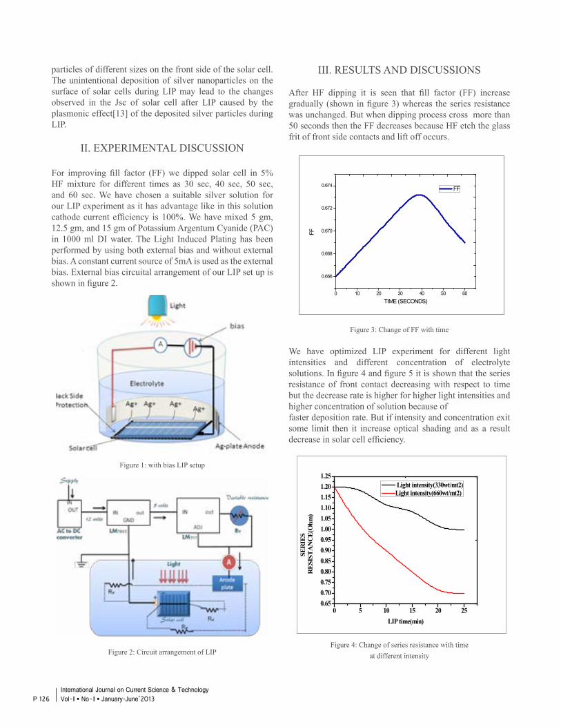
particles of different sizes on the front side of the solar cell. The unintentional deposition of silver nanoparticles on the surface of solar cells during LIP may lead to the changes observed in the Jsc of solar cell after LIP caused by the plasmonic effect[13] of the deposited silver particles during LIP.
II. EXPERIMENTAL DISCUSSION
For improving fill factor (FF) we dipped solar cell in 5% HF mixture for different times as 30 sec, 40 sec, 50 sec, and 60 sec. We have chosen a suitable silver solution for our LIP experiment as it has advantage like in this solution cathode current efficiency is 100%. We have mixed 5 gm, 12.5 gm, and 15 gm of Potassium Argentum Cyanide (PAC) in 1000 ml DI water. The Light Induced Plating has been performed by using both external bias and without external bias. A constant current source of 5mA is used as the external bias. External bias circuital arrangement of our LIP set up is shown in figure 2.
Figure 1: with bias LIP setup
Figure 2: Circuit arrangement of LIP
III. RESULTS AND DISCUSSIONS
After HF dipping it is seen that fill factor (FF) increase gradually (shown in figure 3) whereas the series resistance was unchanged. But when dipping process cross more than 50 seconds then the FF decreases because HF etch the glass frit of front side contacts and lift off occurs.
Figure 3: Change of FF with time
We have optimized LIP experiment for different light intensities and different concentration of electrolyte solutions. In figure 4 and figure 5 it is shown that the series resistance of front contact decreasing with respect to time but the decrease rate is higher for higher light intensities and higher concentration of solution because offaster deposition rate. But if intensity and concentration exit some limit then it increase optical shading and as a result decrease in solar cell efficiency.
Figure 4: Change of series resistance with timeat different intensity
0 10 20 30 40 50 60
0.666
0.668
0.670
0.672
0.674
FF
TIME (SECONDS)
FF
0 5 10 15 20 250.650.700.750.800.850.900.951.001.051.101.151.201.25
SER
IES
RES
ISTA
NC
E(O
hm)
LIP time(min)
Light intensity(330wt/mt2)Light intensity(660wt/mt2)
P 126International Journal on Current Science & Technology Vol - I l No- I l January-June’2013
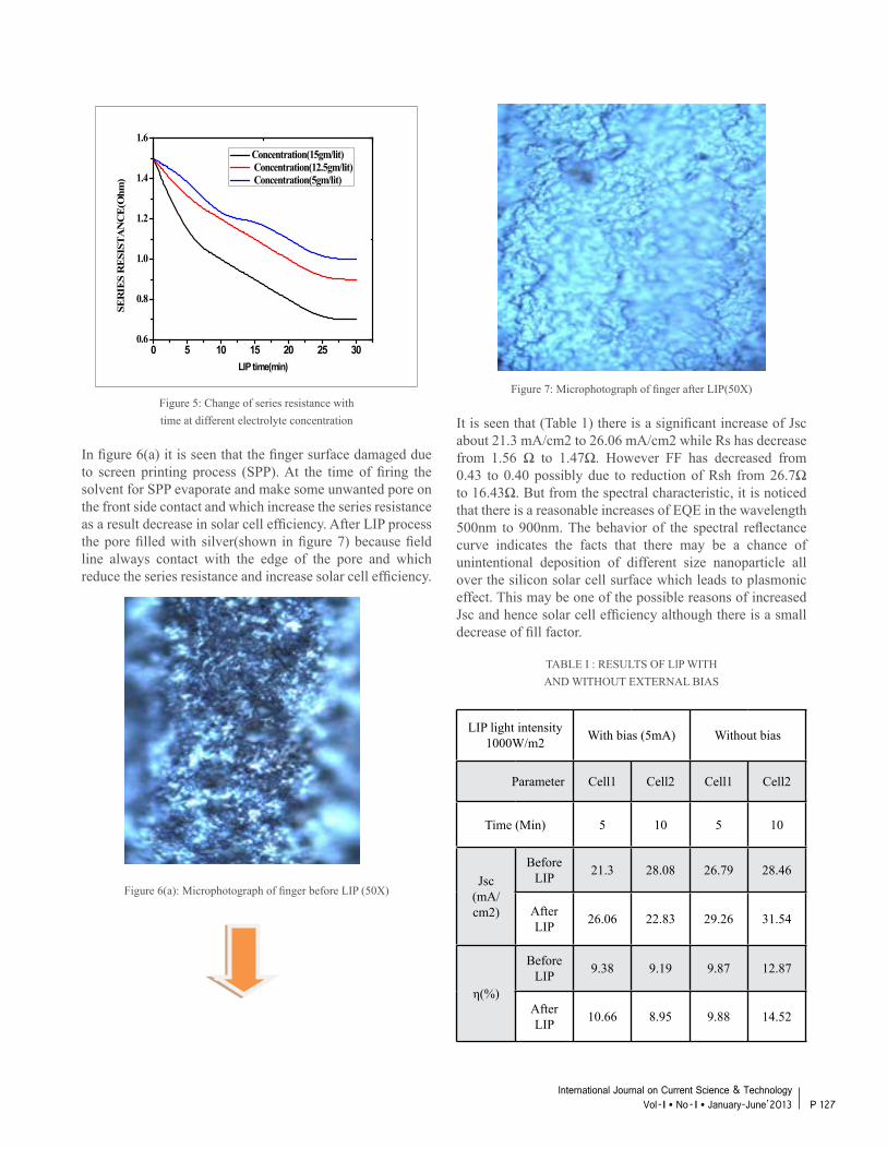
Figure 5: Change of series resistance withtime at different electrolyte concentration
In figure 6(a) it is seen that the finger surface damaged due to screen printing process (SPP). At the time of firing the solvent for SPP evaporate and make some unwanted pore on the front side contact and which increase the series resistance as a result decrease in solar cell efficiency. After LIP process the pore filled with silver(shown in figure 7) because field line always contact with the edge of the pore and which reduce the series resistance and increase solar cell efficiency.
Figure 6(a): Microphotograph of finger before LIP (50X)
0 5 10 15 20 25 300.6
0.8
1.0
1.2
1.4
1.6 Concentration(15gm/lit) Concentration(12.5gm/lit) Concentration(5gm/lit)
SER
IES
RE
SIST
AN
CE
(Ohm
)
LIP time(min)
Figure 7: Microphotograph of finger after LIP(50X)
It is seen that (Table 1) there is a significant increase of Jsc about 21.3 mA/cm2 to 26.06 mA/cm2 while Rs has decrease from 1.56 Ω to 1.47Ω. However FF has decreased from 0.43 to 0.40 possibly due to reduction of Rsh from 26.7Ω to 16.43Ω. But from the spectral characteristic, it is noticed that there is a reasonable increases of EQE in the wavelength 500nm to 900nm. The behavior of the spectral reflectance curve indicates the facts that there may be a chance of unintentional deposition of different size nanoparticle all over the silicon solar cell surface which leads to plasmonic effect. This may be one of the possible reasons of increased Jsc and hence solar cell efficiency although there is a small decrease of fill factor.
TABLE I : RESULTS OF LlP WITHAND WITHOUT EXTERNAL BIAS
LIP light intensity 1000W/m2 With bias (5mA) Without bias
Parameter Cell1 Cell2 Cell1 Cell2
Time (Min) 5 10 5 10
Jsc (mA/cm2)
Before LIP 21.3 28.08 26.79 28.46
After LIP 26.06 22.83 29.26 31.54
η(%)
Before LIP 9.38 9.19 9.87 12.87
After LIP 10.66 8.95 9.88 14.52
P 127International Journal on Current Science & Technology
Vol - I l No- I l January-June’2013
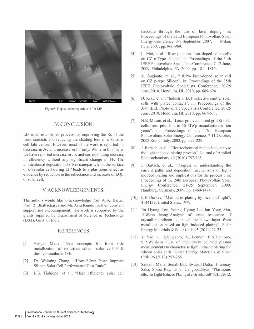
Figure8: Deposited nanoparticles after LIP
IV. CONCLUSION:
LIP is an established process for improving the Rs of the front contacts and reducing the shading loss in c-Si solar cell fabrication. However, most of the work is reported on decrease in Jsc and increase in FF only. While in this paper we have reported increase in Jsc and corresponding increase in efficiency without any significant change in FF. The unintentional deposition of silver nanoparticle on the surface of c-Si solar cell during LIP leads to a plasmonic effect as evidence by reduction in the reflectance and increase of EQE of solar cell.
V. ACKNOWLEDGEMENTS:
The authors would like to acknowledge Prof. A. K. Barua, Prof. R. Bhattacharya and Mr. Avra Kundu for their constant support and encouragement. The work is supported by the grants supplied by Department of Science & Technology (DST), Govt. of India
REFERENCES
[1 Ansgar Mette “New concepts for front side metallization of industrial silicon solar cells”PhD thesis, Fraunhofer-ISE.
[2] Dr. Weiming Zhang “How Silver Paste Improve Silicon Solar Cell Performance/Cost Ratio”
[3] B.S. Tjahjono, et al., “High efficiency solar cell
structure through the use of laser doping” in: Proceedings of the 22nd European Photovoltaic Solar Energy Conference, 3-7 September, 2007, Milan, Italy, 2007, pp. 966-969.
[4] L. Mai, et al. “Rear junction laser doped solar cells on CZ n-Type silicon”, in: Proceedings of the 34th IEEE Photovoltaic Specialists Conference, 7-12 June, 2009, Philadelphia, PA, 2009, pp. 1811-1815.
[5] A. Sugianto, et al., “18.5% laser-doped solar cell on CZ p-type Silicon”, in: Proceedings of the 35th IEEE Photovoltaic Specialists Conference, 20-25 June, 2010, Honolulu, HI, 2010, pp. 689-694.
[6] D. Kray, et al., “Industrial LCP selective emitter solar cells with plated contacts”, in: Proceedings of the 35th IEEE Photovoltaic Specialists Conference, 20-25 June, 2010, Honolulu, HI, 2010, pp. 667-671.
[7] N.B. Mason, et al., “Laser grooved buried grid Si solar cells from pilot line to 50 MWp manufacture in ten years”, in: Proceedings of the 17th European Photovoltaic Solar Energy Conference, 7-11 October, 2002 Rome, Italy, 2002, pp. 227-229.
[8] J. Bartsch, et al., “Electrochemical methods to analyse the light-induced plating process”, Journal of Applied Electrochemistry 40 (2010) 757-765.
[9] J. Bartsch, et al., “Progress in understanding the current paths and deposition mechanisms of light- induced plating and implications for the process”, in: Proceedings of the 24th European Photovoltaic Solar Energy Conference, 21-25 September, 2009, Hamburg, Germany, 2009, pp. 1469-1474.
[10] L.F. Durkee, “Method of plating by means of light”, 4144139, United States, 1979.
[11] Jin Hyung Lee, Young Hyung Lee,Jun Yong Ahn, Ji-Weon Jeong“Analysis of series resistance of crystalline silicon solar cell with two-layer front metallization based on light-induced plating”, Solar Energy Materials & Solar Cells 95 (2011) 22-25.
[12] Y. Yao n, A.Sugianto, A.J.Lennon, B.S.Tjahjono, S.R.Wenham “Use of inductively coupled plasma measurements to characterise light induced plating for silicon solar cells” Solar Energy Materials & Solar Cells 96 (2012) 257-265.
[13] Santanu Maity, Sonali Das, Swapan Datta, Hiranmay Saha, Soma Ray, Utpal Gangopadhyay “Plasmonic effect in Light-Induced Plating of c-Si solar cell” ICEE 2012.
P 128International Journal on Current Science & Technology Vol - I l No- I l January-June’2013
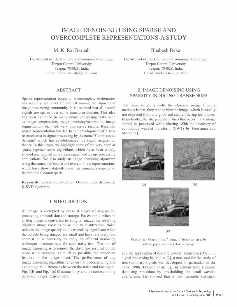
IMAGE DENOISING USING SPARSE AND OVERCOMPLETE REPRESENTATIONS-A STUDY
Bhabesh Deka
Department of Electronics and Communication Engg. Tezpur Central University
Tezpur, 784028, India Email: [email protected]
M. K. Rai Baruah
Department of Electronics and Communication Engg. Tezpur Central University
Tezpur, 784028, India Email: [email protected]
ABSTRACT
Sparse representation based on overcomplete dictionaries has recently got a lot of interest among the signal and image processing community. It is assumed that all natural signals are sparse over some transform domain. This idea has been exploited in many image processing tasks such as image compression, image denoising/restoration, image segmentation, etc. with very impressive results. Recently, sparse representation has led to the development of a new research area in signal processing by the name ”Compressive Sensing” which has revolutionized the signal acquisition theory. In this paper, we highlight some of the very popular sparse representation algorithms which have been widely studied and applied for various signal and image processing applications. We also study an image denoising algorithm using the concept of sparse and overcomplete representations which have shown state-of-the-art performance compared to its traditional counterparts.
Keywords : Sparse representation, Overcomplete dictionary, K-SVD algorithm
I. NTRODUCTION
An image is corrupted by noise at stages of acquisition, processing, transmission and storage. For example, when an analog image is converted to a digital image, the resulting digitized image contains noise due to quantization. Noise reduces the image quality and is especially significant when the objects being imaged are small and have relatively low contrast. It is necessary to apply an efficient denoising technique to compensate for such noisy data. The aim of image denoising is to remove the distortion resulted by the noise while keeping, as much as possible, the important features of the image intact. The performance of any image denoising algorithm relies on the understanding and exploiting the differences between the noise and the signal. Fig. 1(b) and Fig. 1(c) illustrate noisy and the corresponding denoised images, respectively.
II. IMAGE DENOISING USINGSPARSITY INDUCING TRANSFORMS
The basic difficulty with the classical image filtering methods is that, they tend to blur the image, which is usually not expected from any good and stable filtering techniques. In particular, the sharp edges or lines that occur in the image should be preserved while filtering. With the discovery of continuous wavelet transform (CWT) by Grossman and Morlet [1]
(a) (b)
(c)
Figure 1. (a) Original “Boat” image. (b) Image corrupted bysalt and pepper noise. (c) Denoised image
and the application of discrete wavelet transform (DWT) in signal processing by Mallat [2], a new tool for the study of non-stationary signals was developed. In particular, in the early 1990s, Donoho et al. [3], [4] demonstrated a simple denoising procedure by thresholding the detail wavelet coefficients. He showed that it had desirable statistical
P 129International Journal on Current Science & Technology
Vol - I l No- I l January-June’2013
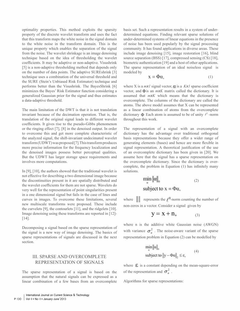
optimality properties. This method exploits the sparsity property of the discrete wavelet transform and uses the fact that this transform maps the white noise in the signal domain to the white noise in the transform domain. This is the unique property which enables the separation of the signal from the noise. The wavelet shrinkage is an image denoising technique based on the idea of thresholding the wavelet coefficients. It may be adaptive or non-adaptive. Visushrink [5] is a non-adaptive thresholding method that depends only on the number of data points. The adaptive SUREshrink [3] technique uses a combination of the universal threshold and the SURE (Stein’s Unbiased Risk Estimator) technique and performs better than the Visushrink. The BayesShrink [6] minimizes the Bayes’ Risk Estimator function considering a generalized Gaussian prior for the signal and thus estimates a data-adaptive threshold.
The main limitation of the DWT is that it is not translation invariant because of the decimation operation. That is, the translation of the original signal leads to different wavelet coefficients. It gives rise to the pseudo-Gibbs phenomenon or the ringing effect [7], [8] in the denoised output. In order to overcome this and get more complete characteristic of the analyzed signal, the shift-invariant undecimated wavelet transform (UDWT) was proposed [7].This transform produces more precise information for the frequency localization and the denoised images possess better perceptual qualities. But the UDWT has larger storage space requirements and involves more computations.
In [9], [10], the authors showed that the traditional wavelet is not effective for describing a two dimensional image because the discontinuities present in it are spatially distributed and the wavelet coefficients for them are not sparse. Wavelets do very well for the representation of point singularities present in a one dimensional signal but fails in the case of lines and curves in images. To overcome these limitations, several new multiscale transforms were proposed. These include the curvelets [9], the contourlets [11], and the ridgelets [10]. Image denoising using these transforms are reported in [12]-[14].
Decomposing a signal based on the sparse representation of the signal is a new way of image denoising. The basics of sparse representations of signals are discussed in the next section.
III. SPARSE AND OVERCOMPLETE REPRESENTATION OF SIGNALS
The sparse representation of a signal is based on the assumption that the natural signals can be expressed as a linear combination of a few bases from an overcomplete
basis set. Such a representation results in a system of under-determined equations. Finding relevant sparse solutions of under-determined systems of linear equations in the presence of noise has been used popularly by the signal processing community. It has found applications in diverse areas. These include image denoising [15], image restoration [16], blind source separation (BSS) [17], compressed sensing (CS) [18], biometric authentication [19] and a host of other applications.The sparse representation of an ideal noiseless signal is modeled by (1)
where X is a mx1 signal vector, is a Kx1 sparse coefficient vector, and is an mxK matrix called the dictionary. It is assumed that mxK which means that the dictionary is overcomplete. The columns of the dictionary are called the atoms. The above model assumes that X can be represented as a linear combination of atoms from the overcomplete dictionary . Each atom is assumed to be of unity -norm throughout this work.
The representation of a signal with an overcomplete dictionary has the advantage over traditional orthogonal basis representations because they offer a wider range of generating elements (bases) and hence are more flexible in signal representation. A theoretical justification of the use of an overcomplete dictionary has been given in [20]. We assume here that the signal has a sparse representation on the overcomplete dictionary. Since the dictionary is over-complete, the problem in Equation (1) has infinitely many solutions.
(2)
where represents the -norm counting the number of non-zeros in a vector. Consider a signal given by
(3) where n is the additive white Gaussian noise (AWGN) with variance . The noise-aware variant of the sparse representation problem in Equation (2) can be modelled by
(4)
where is a constant depending on the mean-square-error of the representation and .
Algorithms for sparse representations:
2
0
y x n,= +
2nσ
2nσ
P 130International Journal on Current Science & Technology Vol - I l No- I l January-June’2013
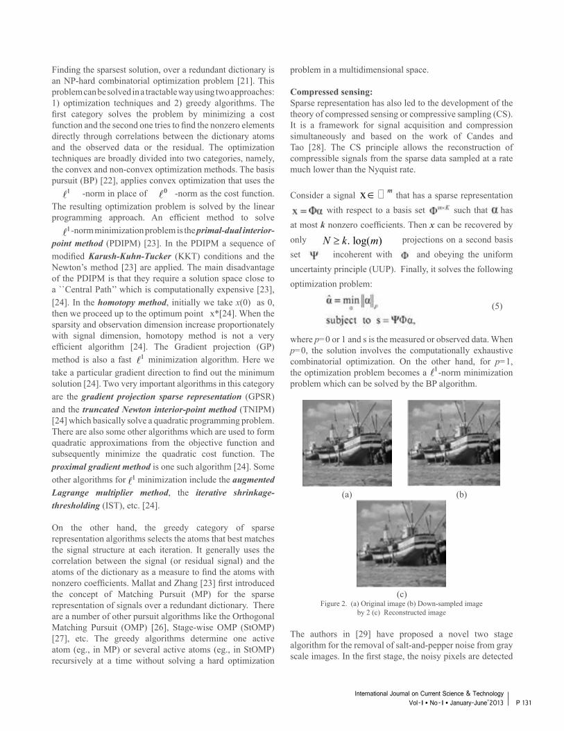
Finding the sparsest solution, over a redundant dictionary is an NP-hard combinatorial optimization problem [21]. This problem can be solved in a tractable way using two approaches: 1) optimization techniques and 2) greedy algorithms. The first category solves the problem by minimizing a cost function and the second one tries to find the nonzero elements directly through correlations between the dictionary atoms and the observed data or the residual. The optimization techniques are broadly divided into two categories, namely, the convex and non-convex optimization methods. The basis pursuit (BP) [22], applies convex optimization that uses the -norm in place of -norm as the cost function. The resulting optimization problem is solved by the linear programming approach. An efficient method to solve -norm minimization problem is the primal-dual interior-point method (PDIPM) [23]. In the PDIPM a sequence of modified Karush-Kuhn-Tucker (KKT) conditions and the Newton’s method [23] are applied. The main disadvantage of the PDIPM is that they require a solution space close to a ``Central Path’’ which is computationally expensive [23], [24]. In the homotopy method, initially we take x(0) as 0, then we proceed up to the optimum point x*[24]. When the sparsity and observation dimension increase proportionately with signal dimension, homotopy method is not a very efficient algorithm [24]. The Gradient projection (GP) method is also a fast minimization algorithm. Here we take a particular gradient direction to find out the minimum solution [24]. Two very important algorithms in this category are the gradient projection sparse representation (GPSR) and the truncated Newton interior-point method (TNIPM) [24] which basically solve a quadratic programming problem. There are also some other algorithms which are used to form quadratic approximations from the objective function and subsequently minimize the quadratic cost function. The proximal gradient method is one such algorithm [24]. Some other algorithms for minimization include the augmented Lagrange multiplier method, the iterative shrinkage-thresholding (IST), etc. [24].
On the other hand, the greedy category of sparse representation algorithms selects the atoms that best matches the signal structure at each iteration. It generally uses the correlation between the signal (or residual signal) and the atoms of the dictionary as a measure to find the atoms with nonzero coefficients. Mallat and Zhang [23] first introduced the concept of Matching Pursuit (MP) for the sparse representation of signals over a redundant dictionary. There are a number of other pursuit algorithms like the Orthogonal Matching Pursuit (OMP) [26], Stage-wise OMP (StOMP) [27], etc. The greedy algorithms determine one active atom (eg., in MP) or several active atoms (eg., in StOMP) recursively at a time without solving a hard optimization
problem in a multidimensional space.
Compressed sensing:Sparse representation has also led to the development of the theory of compressed sensing or compressive sampling (CS). It is a framework for signal acquisition and compression simultaneously and based on the work of Candes and Tao [28]. The CS principle allows the reconstruction of compressible signals from the sparse data sampled at a rate much lower than the Nyquist rate.
Consider a signal that has a sparse representation with respect to a basis set such that has at most k nonzero coefficients. Then x can be recovered by only projections on a second basis set incoherent with and obeying the uniform uncertainty principle (UUP). Finally, it solves the following optimization problem:
(5)
where p=0 or 1 and s is the measured or observed data. When p=0, the solution involves the computationally exhaustive combinatorial optimization. On the other hand, for p=1, the optimization problem becomes a -norm minimization problem which can be solved by the BP algorithm.
(a) (b)
(c)Figure 2. (a) Original image (b) Down-sampled image
by 2 (c) Reconstructed image
The authors in [29] have proposed a novel two stage algorithm for the removal of salt-and-pepper noise from gray scale images. In the first stage, the noisy pixels are detected
01
1
11
1
x m∈
. log( )N k m≥
P 131International Journal on Current Science & Technology
Vol - I l No- I l January-June’2013
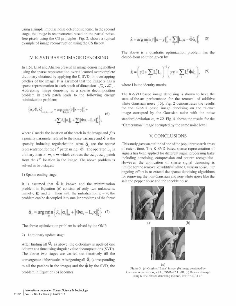
(8)
The above is a quadratic optimization problem has the closed-form solution given by
(9)
where I is the identity matrix.
The K-SVD based image denoising is shown to have the state-of-the-art performance for the removal of additive white Gaussian noise [15]. Fig. 2 demonstrates the results for the K-SVD based image denoising on the “Lena” image corrupted by the Gaussian noise with the noise standard deviation .Fig. 4. shows the results for the “Cameraman” image corrupted by the same noise level.
V. CONCLUSIONS
This study gave an outline of one of the popular research areas of recent time. The K-SVD based sparse representation of signals has been applied for different signal processing tasks including denoising, compression and pattern recognition. However, the application of sparse signal denoising is limited for the removal of additive white Gaussian noise. Our ongoing effort is to extend the sparse denoising algorithms for removing the non-Gaussian and non-white noise like the salt and pepper noise and the speckle noise.
a) (b)
(c)
Figure 3. (a) Original “Lena” image. (b) Image corrupted byGaussian noise with , PSNR=22.11 dB. (c) Denoised image
using K-SVD based denoising method, PSNR=32.31 dB.
using a simple impulse noise detection scheme. In the second stage, the image is reconstructed based on the partial noise-free pixels using the CS principles. Fig. 2. shows a typical example of image reconstruction using the CS theory.
IV. K-SVD BASED IMAGE DENOISING
In [15], Elad and Aharon present an image denoising method using the sparse representation over a learned overcomplete dictionary obtained by applying the K-SVD, on overlapping patches of the image. It is assumed that the image x has a sparse representation in each patch of dimension . Addressing image denoising as a sparse decomposition problem in each patch leads to the following energy minimization problem:
(6)
where i marks the location of the patch in the image and is a penalty parameter related to the noise variance and is the sparsity inducing regularization term. are the sparse representation for the i th patch using . The operator L i is a binary matrix which extracts the patch from the i th location in the image. The above problem is solved in two stages:
1) Sparse coding stage
It is assumed that is known and the minimization problem in Equation (6) consists of only two unknowns, namely, and x . Then with the initialization x = y, the problem can be decoupled into smaller problems of the form:
(7)
The above optimization problem is solved by the OMP.
2) Dictionary update stage
After finding all as above, the dictionary is updated one column at a time using singular value decompositions (SVD). The above two stages are carried out iteratively till the convergence of the results. After getting all (corresponding to all the patches in the image) and the by the SVD, the problem in Equation (6) becomes
p pm m×
p pm m×
γλ
pm m×
20nσ =
20nσ =
P 132International Journal on Current Science & Technology Vol - I l No- I l January-June’2013
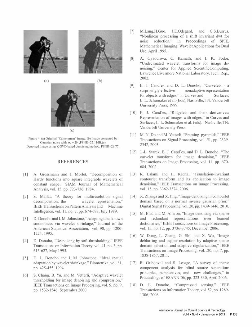
(a) (b)
(c)
Figure 4. (a) Original “Cameraman” image. (b) Image corrupted byGaussian noise with ,PSNR=22.11dB.(c)
Denoised image using K-SVD based denoising method, PSNR=29.77.
REFERENCES
[1] A. Grossmann and J. Morlet, “Decomposition of Hardy functions into square integrable wavelets of constant shape,” SIAM Journal of Mathematical Analysis, vol. 15, pp. 723-736, 1984.
[2] S. Mallat, “A theory for multiresolution signal decomposition: the wavelet representation,” IEEE Transactions on Pattern Analysis and Machine Intelligence, vol. 11, no. 7, pp. 674-693, July 1989.
[3] D. Donoho and I. M. Johnstone, “Adapting to unknown smoothness via wavelet shrinkage,” Journal of the American Statistical Association, vol. 90, pp. 1200- 1224, 1995.
[4] D. Donoho, “De-noising by soft-thresholding,” IEEE Transactions on Information Theory, vol. 41, no. 3, pp. 613-627, May 1995.
[5] D. L. Donoho and I. M. Johnstone, “Ideal spatial adaptation by wavelet shrinkage,” Biometrika, vol. 81, pp. 425-455, 1994.
[6] S. Chang, B. Yu, and M. Vetterli, “Adaptive wavelet thresholding for image denoising and compression,” IEEE Transactions on Image Processing, vol. 9, no. 9, pp. 1532-1546, September 2000.
[7] M.Lang,H.Guo, J.E.Odegard, and C.S.Burrus, “Nonlinear processing of a shift invariant dwt for noise reduction,” in Proceedings of SPIE, Mathematical Imaging: Wavelet Applications for Dual Use, April 1995.
[8] A. Gyaourova, C. Kamath, and I. K. Fodor, “Undecimated wavelet transforms for image de- noising,” Center for Applied ScientificComputing, Lawrence Livermore National Laboratory, Tech. Rep., 2002.
[9] E. J. Cand`es and D. L. Donoho, “Curvelets - a surprisingly effective nonadaptive representation for objects with edges,” in Curves and Surfaces, L. L. Schumaker et al. (Eds). Nashville, TN: Vanderbilt University Press, 1999.
[10] E. J. Cand`es, “Ridgelets and their derivatives: Representation of images with edges,” in Curves and Surfaces, L. L. Schumaker et al. (eds). Nashville, TN: Vanderbilt University Press.
[11] M. N. Do and M. Vetterli, “Framing pyramids,” IEEE Transactions on Signal Processing, vol. 51, pp. 2329- 2342, 2003.
[12] J.-L. Starck, E. J. Cand`es, and D. L. Donoho, “The curvelet transform for image denoising,” IEEE Transactions on Image Processing, vol. 11, pp. 670- 684, 2002.
[13] R. Eslami and H. Radha, “Translation-invariant contourlet transform and its application to image denoising,” IEEE Transactions on Image Processing, vol. 15, pp. 3362-3374, 2006.
[14] X. Zhanga and X. Jing, “Image denoising in contourlet domain based on a normal inverse gaussian prior,” Digital Signal Processing, vol. 20, pp. 1439-1446, 2010.
[15] M. Elad and M. Aharon, “Image denoising via sparse and redundant representations over learned dictionaries,” IEEE Transactions on Image Processing, vol. 15, no. 12, pp. 3736-3745, December 2006.
[16] W. Dong, L. Zhang, G. Shi, and X. Wu, “Image deblurring and supper-resolution by adaptive sparse domain selection and adaptive regularization,” IEEE Transactions on Image Processing, vol. .20, no. 7, pp. 1838-1857, 2011.
[17] R. Gribonval and S. Lesage, “A survey of sparse component analysis for blind source separation: principles, perspectives, and new challenges,” in Proceedings of ESANN’06, pp. 323-330, April 2006.
[18] D. L. Donoho, “Compressed sensing,” IEEE Transactions on Information Theory, vol. 52, pp. 1289- 1306, 2006.
20nσ =
P 133International Journal on Current Science & Technology
Vol - I l No- I l January-June’2013
[19] J. K. Pillai, V. M. Patel, R. Chellappa, and N. K. Ratha, “Secure and robust iris recognition using random projections and sparse representations,”IEEE Transactions on Pattern Analysis and Machine Intelligence, IEEE Computer Society, 2011, 33, 1877-1893.
[20] B. A. Olshausen and D. J. Field, “Sparse coding with an overcomplete basis set: A strategy employed by V1?”VisionResearch, vol. 37, no. 23, pp. 3311- 3325, 1997.
[21] G. Davis, S. Mallat, and M. Avellaneda, “Adaptive greedy approximations,”Journal of Constructive Approximation, vol. 13, pp. 57-98, 1997.
[22] S. S. Chen, D. L. Donoho, and M. A. Saunders, “Atomic decomposition by basis pursuit,” SIAM Journal on Scientific Computing, vol. 20, no. 1, pp. 33-61, 1998.
[23] S. Boyd and L. Vandenberghe, Convex Optimization. New York, NY, USA: Cambridge University Press, 2004.
[24] A. Y. Yang, A. Ganesh, Z. Zhou, S. S. Sastry, and Y. Ma,“A review of fast l1-minimization algorithms for robust face recognition,” EECS Department, University of California, Berkeley, http://www.eecs. berkeley.edu/Pubs/TechRpts/2010/EECS-2010-13.
html, Tech. Rep., Feb. 2010.
[25] S. Mallat and Z. Zhang, “Matching pursuits with time-frequency dictionaries,”IEEE Transactions on Signal Processing, vol. 41, no. 12, pp.3397-3415, December 1993.
[26] Y. Pati, R. Rezaiifar, and P. Krishnaprasad, “Orthogonal matching pursuit: recursive function approximation with applications to wavelet decomposition,” in Proceedings of the 27th Annual Asilomer conference on Signals, Systems, and Computers,, pp. 40-44, 1993.
[27] D. L. Donoho, Y. Tsaig, I. Drori, and J. luc Starck, “Sparse solution of underdetermined linear equations by stagewise orthogonal matching pursuit,”Tech. Rep., 2006. [Online]. Available :http://wwwstat. standford.edu/~idrori/STOMP.pdf
[28] E. J. Cand`es and T. Tao, “Near-optimal signal recovery from random projections: universal encoding strategies,” IEEE Transactions on Information Theory, vol. 52, pp. 5406-5425, December 2006.
[29] H. Huang and J. Zhu, “Removal of salt-and-pepper noise based on compressed sensing,” Electronics Letters, vol. 46, pp. 1198-1199, August 2010.
P 134International Journal on Current Science & Technology Vol - I l No- I l January-June’2013
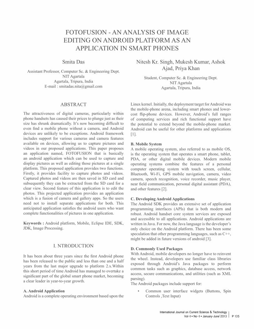
FOTOFUSION - AN ANALYSIS OF IMAGEEDITING ON ANDROID PLATFORM AS AN
APPLICATION IN SMART PHONES
Smita Das
Assistant Professor, Computer Sc. & Engineering Dept.NIT Agartala
Agartala, Tripura, IndiaE-mail : [email protected]
Nitesh Kr. Singh, Mukesh Kumar, Ashok Ajad, Priya Khan
Student, Computer Sc. & Engineering Dept.NIT Agartala
Agartala, Tripura, India
ABSTRACT
The attractiveness of digital cameras, particularly within phone handsets has caused their prices to plunge just as their size has shrunk dramatically. It’s now becoming difficult to even find a mobile phone without a camera, and Android devices are unlikely to be exceptions. Android framework includes support for various cameras and camera features available on devices, allowing us to capture pictures and videos in our proposed applications. This paper proposes an application named, FOTOFUSION that is basically an android application which can be used to capture and display pictures as well as editing those pictures at a single platform. This proposed application provides two functions. Firstly, it provides facility to capture photos and videos. Captured photos and videos are then saved in SD card and subsequently they can be extracted from the SD card for a clear view. Second feature of this application is to edit the photos. This projected application provides an application which is a fusion of camera and gallery apps. So the users need not to install separate applications for both. This anticipated application satisfies the android users who want complete functionalities of pictures in one application.
Keywords : Android platform, Mobile, Eclipse IDE, SDK, JDK, Image Processing.
I. NTRODUCTION
It has been about three years since the first Android phone has been released to the public and less than one and a half years from the last major upgrade to platform 2.x.Within this short period of time Android has managed to overtake a significant part of the global smart phone market, becoming a clear leader in year-to-year growth.
A. Android ApplicationAndroid is a complete operating environment based upon the
Linux kernel. Initially, the deployment target for Android was the mobile-phone arena, including smart phones and lower-cost flip-phone devices. However, Android’s full ranges of computing services and rich functional support have the potential to extend beyond the mobile-phone market. Android can be useful for other platforms and applications [1].
B. Mobile SystemA mobile operating system, also referred to as mobile OS, is the operating system that operates a smart phone, tablet, PDA, or other digital mobile devices. Modern mobile operating systems combine the features of a personal computer operating system with touch screen, cellular, Bluetooth, Wi-Fi, GPS mobile navigation, camera, video camera, speech recognition, voice recorder, music player, near field communication, personal digital assistant (PDA), and other features [2].
C. Developing Android ApplicationsThe Android SDK provides an extensive set of application programming interfaces (APIs) that is both modern and robust. Android handset core system services are exposed and accessible to all applications. Android applications are written in Java. For now, the Java language is the developer’s only choice on the Android platform. There has been some speculation that other programming languages, such as C++, might be added in future versions of android [3].
D. Commonly Used PackagesWith Android, mobile developers no longer have to reinvent the wheel. Instead, developers use familiar class libraries exposed through Android’s Java packages to perform common tasks such as graphics, database access, network access, secure communications, and utilities (such as XML parsing).The Android packages include support for:
• Common user interface widgets (Buttons, Spin Controls ,Text Input)
P 135International Journal on Current Science & Technology
Vol - I l No- I l January-June’2013
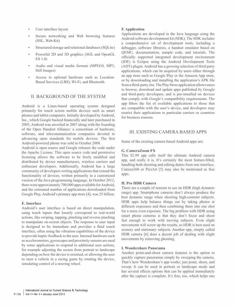
• User interface layout
• Secure networking and Web browsing features (SSL, Web-Kit)
• Structured storage and relational databases (SQLite)
• Powerful 2D and 3D graphics (SGL and OpenGL ES 1.0)
• Audio and visual media formats (MPEG4, MP3, Still Images)
• Access to optional hardware such as Location- Based Services (LBS), Wi-Fi, and Bluetooth.
II. BACKGROUND OF THE SYSTEM
Android is a Linux-based operating system designed primarily for touch screen mobile devices such as smart phones and tablet computers. Initially developed by Android, Inc., which Google backed financially and later purchased in 2005, Android was unveiled in 2007 along with the founding of the Open Handset Alliance: a consortium of hardware, software, and telecommunication companies devoted to advancing open standards for mobile devices. The first Android-powered phone was sold in October 2008.Android is open source and Google releases the code under the Apache License. This open source code and permissive licensing allows the software to be freely modified and distributed by device manufacturers, wireless carriers and enthusiast developers. Additionally, Android has a large community of developers writing applications that extend the functionality of devices, written primarily in a customized version of the Java programming language. In October 2012, there were approximately 700,000 apps available for Android, and the estimated number of applications downloaded from Google Play, Android’s primary app store [4], was 25 billion.
E. InterfaceAndroid’s user interface is based on direct manipulation, using touch inputs that loosely correspond to real-world actions, like swiping, tapping, pinching and reverse pinching to manipulate on-screen objects. The response to user input is designed to be immediate and provides a fluid touch interface, often using the vibration capabilities of the device to provide haptic feedback to the user. Internal hardware such as accelerometers, gyroscopes and proximity sensors are used by some applications to respond to additional user actions, for example adjusting the screen from portrait to landscape depending on how the device is oriented, or allowing the user to steer a vehicle in a racing game by rotating the device, simulating control of a steering wheel.
F. ApplicationApplications are developed in the Java language using the Android software development kit (SDK). The SDK includes a comprehensive set of development tools, including a debugger, software libraries, a handset emulator based on QEMU, documentation, sample code, and tutorials. The officially supported integrated development environment (IDE) is Eclipse using the Android Development Tools (ADT) plugin. Android has a growing selection of third party applications, which can be acquired by users either through an app store such as Google Play or the Amazon App store, or by downloading and installing the application’s APK file from a third-party site. The Play Store application allows users to browse, download and update apps published by Google and third-party developers, and is pre-installed on devices that comply with Google’s compatibility requirements. The app filters the list of available applications to those that are compatible with the user’s device, and developers may restrict their applications to particular carriers or countries for business reasons.
III. EXISTING CAMERA BASED APPS
Some of the existing camera based Android apps are:
G. CameraZoom FXThis $2.99 app calls itself the ultimate Android camera app, and really it is. It’s certainly the most feature-filled, handling both shooting and editing duties from one interface. Camera360 or PicsArt [5] may also be mentioned as free apps.
H. Pro HDR CameraThere are a couple of reasons to use an HDR (high dynamic range) app. Smartphone cameras don’t always produce the best dynamic range when shooting high-contrast subjects. HDR apps help balance things out by taking photos at different exposures and then combining them into one shot for a more even exposure. The big problem with HDR using smart phone cameras is that they don’t focus and shoot fast enough to work with moving subjects. Even slight movements will screw up the results, so HDR is best used on scenery and stationary subjects. Another app, simply called HDR camera [6] does a decent job of dealing with slight movements by removing ghosting.
I. Wondershare PanoramaAnother point-and-shoot camera features is the option to quickly capture panoramas simply by sweeping the camera. That’s how Wondershare’s app works: just point, shoot, and sweep. It can be used in portrait or landscape mode and has several effects options that can be applied immediately after the capture is complete. It’s free, too, which helps one
P 136International Journal on Current Science & Technology Vol - I l No- I l January-June’2013
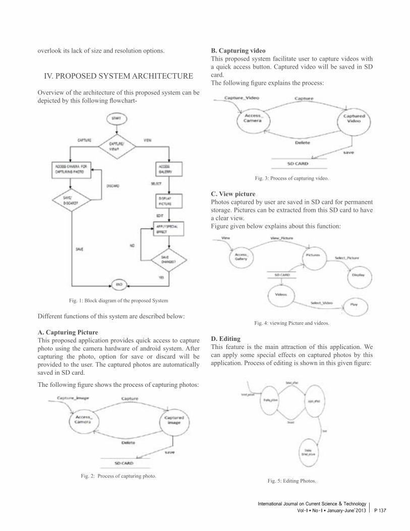
overlook its lack of size and resolution options.
IV. PROPOSED SYSTEM ARCHITECTURE
Overview of the architecture of this proposed system can be depicted by this following flowchart-
Fig. 1: Block diagram of the proposed System
Different functions of this system are described below:
A. Capturing Picture This proposed application provides quick access to capture photo using the camera hardware of android system. After capturing the photo, option for save or discard will be provided to the user. The captured photos are automatically saved in SD card.
The following figure shows the process of capturing photos:
Fig. 2: Process of capturing photo.
B. Capturing videoThis proposed system facilitate user to capture videos with a quick access button. Captured video will be saved in SD card.The following figure explains the process:
Fig. 3: Process of capturing video.
C. View picturePhotos captured by user are saved in SD card for permanent storage. Pictures can be extracted from this SD card to have a clear view.Figure given below explains about this function:
Fig. 4: viewing Picture and videos.
D. EditingThis feature is the main attraction of this application. We can apply some special effects on captured photos by this application. Process of editing is shown in this given figure:
Fig. 5: Editing Photos.
P 137International Journal on Current Science & Technology
Vol - I l No- I l January-June’2013
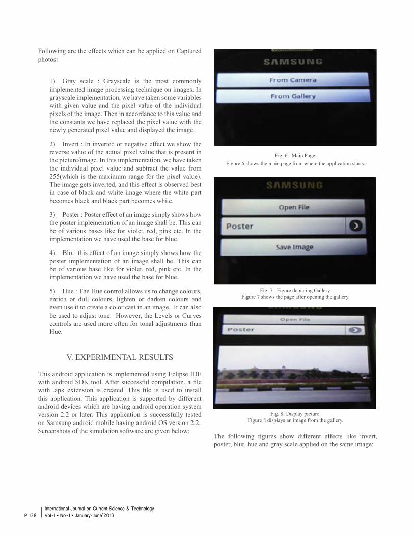
Fig. 6: Main Page.Figure 6 shows the main page from where the application starts.
Fig. 7: Figure depicting Gallery.Figure 7 shows the page after opening the gallery.
Fig. 8: Display picture.Figure 8 displays an image from the gallery.
The following figures show different effects like invert, poster, blur, hue and gray scale applied on the same image:
Following are the effects which can be applied on Captured photos:
1) Gray scale : Grayscale is the most commonly implemented image processing technique on images. In grayscale implementation, we have taken some variables with given value and the pixel value of the individual pixels of the image. Then in accordance to this value and the constants we have replaced the pixel value with the newly generated pixel value and displayed the image.
2) Invert : In inverted or negative effect we show the reverse value of the actual pixel value that is present in the picture/image. In this implementation, we have taken the individual pixel value and subtract the value from 255(which is the maximum range for the pixel value). The image gets inverted, and this effect is observed best in case of black and white image where the white part becomes black and black part becomes white.
3) Poster : Poster effect of an image simply shows how the poster implementation of an image shall be. This can be of various bases like for violet, red, pink etc. In the implementation we have used the base for blue.
4) Blu : this effect of an image simply shows how the poster implementation of an image shall be. This can be of various base like for violet, red, pink etc. In the implementation we have used the base for blue.
5) Hue : The Hue control allows us to change colours, enrich or dull colours, lighten or darken colours and even use it to create a color cast in an image. It can also be used to adjust tone. However, the Levels or Curves controls are used more often for tonal adjustments than Hue.
V. EXPERIMENTAL RESULTS
This android application is implemented using Eclipse IDE with android SDK tool. After successful compilation, a file with .apk extension is created. This file is used to install this application. This application is supported by different android devices which are having android operation system version 2.2 or later. This application is successfully tested on Samsung android mobile having android OS version 2.2.Screenshots of the simulation software are given below:
P 138International Journal on Current Science & Technology Vol - I l No- I l January-June’2013
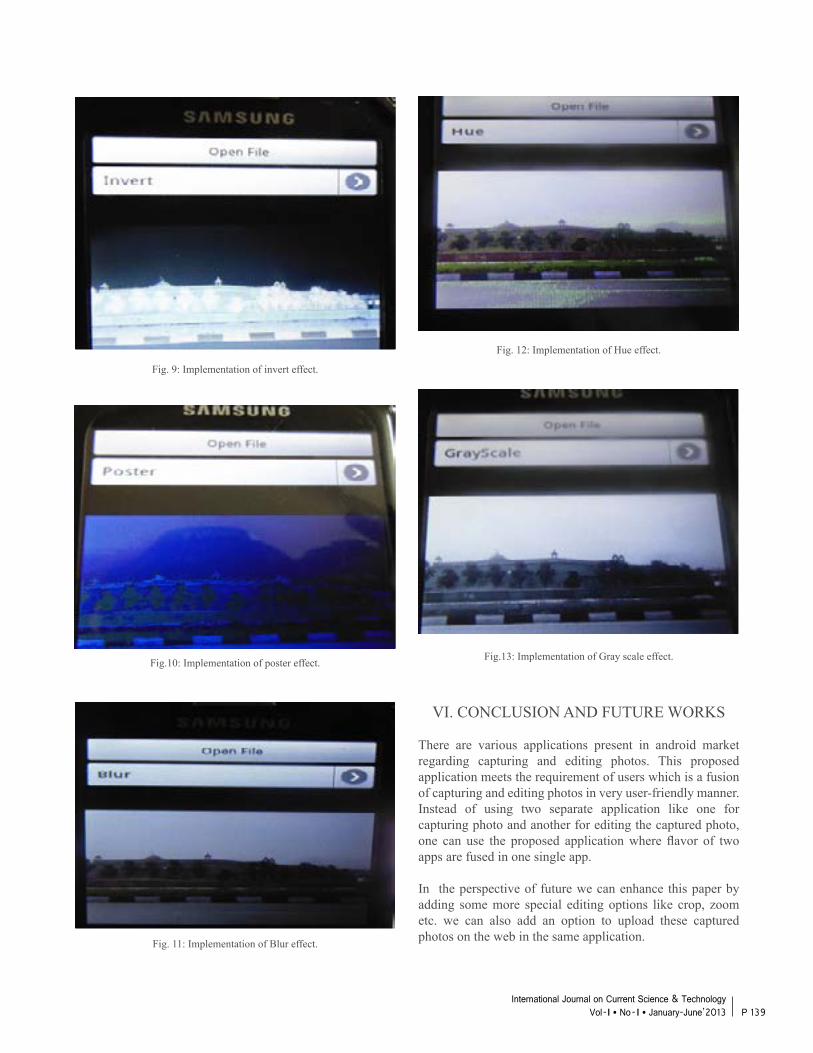
Fig. 9: Implementation of invert effect.
Fig.10: Implementation of poster effect.
Fig. 11: Implementation of Blur effect.
Fig. 12: Implementation of Hue effect.
Fig.13: Implementation of Gray scale effect.
VI. CONCLUSION AND FUTURE WORKS
There are various applications present in android market regarding capturing and editing photos. This proposed application meets the requirement of users which is a fusion of capturing and editing photos in very user-friendly manner. Instead of using two separate application like one for capturing photo and another for editing the captured photo, one can use the proposed application where flavor of two apps are fused in one single app.
In the perspective of future we can enhance this paper by adding some more special editing options like crop, zoom etc. we can also add an option to upload these captured photos on the web in the same application.
P 139International Journal on Current Science & Technology
Vol - I l No- I l January-June’2013

REFERENCES
[1] h t t p : / / w w w . i b m . c o m / d e v e l o p e r w o r k s / library/os-android-devel/J.en.wikipedia.org/wiki/ Mobileoperatingsystem.
[2] h t t p : / / w w w. i n f o r m i t . c o m / a r t i c l e s / a r t i c l e . aspx?p=1388959&seqNum=4.
[3] http://en.wikipedia.org/wiki/Android%28operating_ system%29.
[3] h t tp : / /nad ia -doremisof t .ove r-b log .com/15- categorie-12200732.html.
[4] http://reviews.cnet.com/8301-19736_7-57429313- 251/the-12-best-android-camera-apps-around.
P 140International Journal on Current Science & Technology Vol - I l No- I l January-June’2013
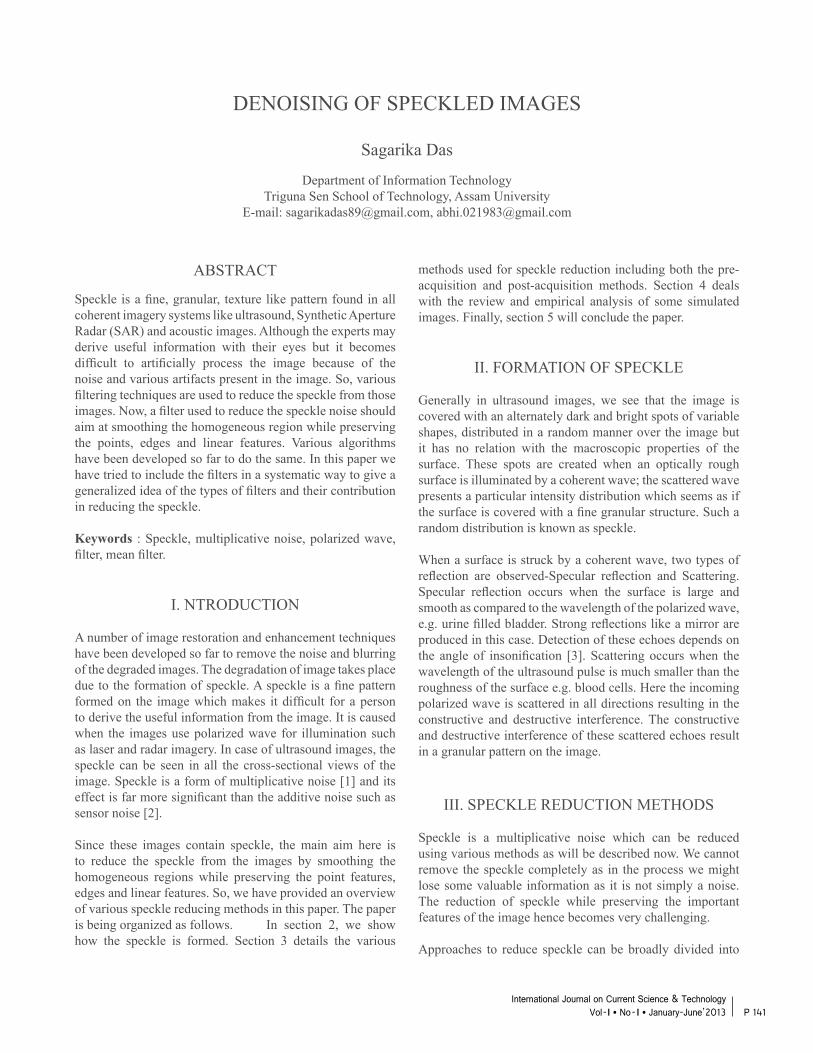
DENOISING OF SPECKLED IMAGES
Sagarika Das
Department of Information TechnologyTriguna Sen School of Technology, Assam University
E-mail: [email protected], [email protected]
ABSTRACT
Speckle is a fine, granular, texture like pattern found in all coherent imagery systems like ultrasound, Synthetic Aperture Radar (SAR) and acoustic images. Although the experts may derive useful information with their eyes but it becomes difficult to artificially process the image because of the noise and various artifacts present in the image. So, various filtering techniques are used to reduce the speckle from those images. Now, a filter used to reduce the speckle noise should aim at smoothing the homogeneous region while preserving the points, edges and linear features. Various algorithms have been developed so far to do the same. In this paper we have tried to include the filters in a systematic way to give a generalized idea of the types of filters and their contribution in reducing the speckle.
Keywords : Speckle, multiplicative noise, polarized wave, filter, mean filter.
I. NTRODUCTION
A number of image restoration and enhancement techniques have been developed so far to remove the noise and blurring of the degraded images. The degradation of image takes place due to the formation of speckle. A speckle is a fine pattern formed on the image which makes it difficult for a person to derive the useful information from the image. It is caused when the images use polarized wave for illumination such as laser and radar imagery. In case of ultrasound images, the speckle can be seen in all the cross-sectional views of the image. Speckle is a form of multiplicative noise [1] and its effect is far more significant than the additive noise such as sensor noise [2].
Since these images contain speckle, the main aim here is to reduce the speckle from the images by smoothing the homogeneous regions while preserving the point features, edges and linear features. So, we have provided an overview of various speckle reducing methods in this paper. The paper is being organized as follows. In section 2, we show how the speckle is formed. Section 3 details the various
methods used for speckle reduction including both the pre-acquisition and post-acquisition methods. Section 4 deals with the review and empirical analysis of some simulated images. Finally, section 5 will conclude the paper.
II. FORMATION OF SPECKLE
Generally in ultrasound images, we see that the image is covered with an alternately dark and bright spots of variable shapes, distributed in a random manner over the image but it has no relation with the macroscopic properties of the surface. These spots are created when an optically rough surface is illuminated by a coherent wave; the scattered wave presents a particular intensity distribution which seems as if the surface is covered with a fine granular structure. Such a random distribution is known as speckle.
When a surface is struck by a coherent wave, two types of reflection are observed-Specular reflection and Scattering. Specular reflection occurs when the surface is large and smooth as compared to the wavelength of the polarized wave, e.g. urine filled bladder. Strong reflections like a mirror are produced in this case. Detection of these echoes depends on the angle of insonification [3]. Scattering occurs when the wavelength of the ultrasound pulse is much smaller than the roughness of the surface e.g. blood cells. Here the incoming polarized wave is scattered in all directions resulting in the constructive and destructive interference. The constructive and destructive interference of these scattered echoes result in a granular pattern on the image.
III. SPECKLE REDUCTION METHODS
Speckle is a multiplicative noise which can be reduced using various methods as will be described now. We cannot remove the speckle completely as in the process we might lose some valuable information as it is not simply a noise. The reduction of speckle while preserving the important features of the image hence becomes very challenging.
Approaches to reduce speckle can be broadly divided into
P 141International Journal on Current Science & Technology
Vol - I l No- I l January-June’2013
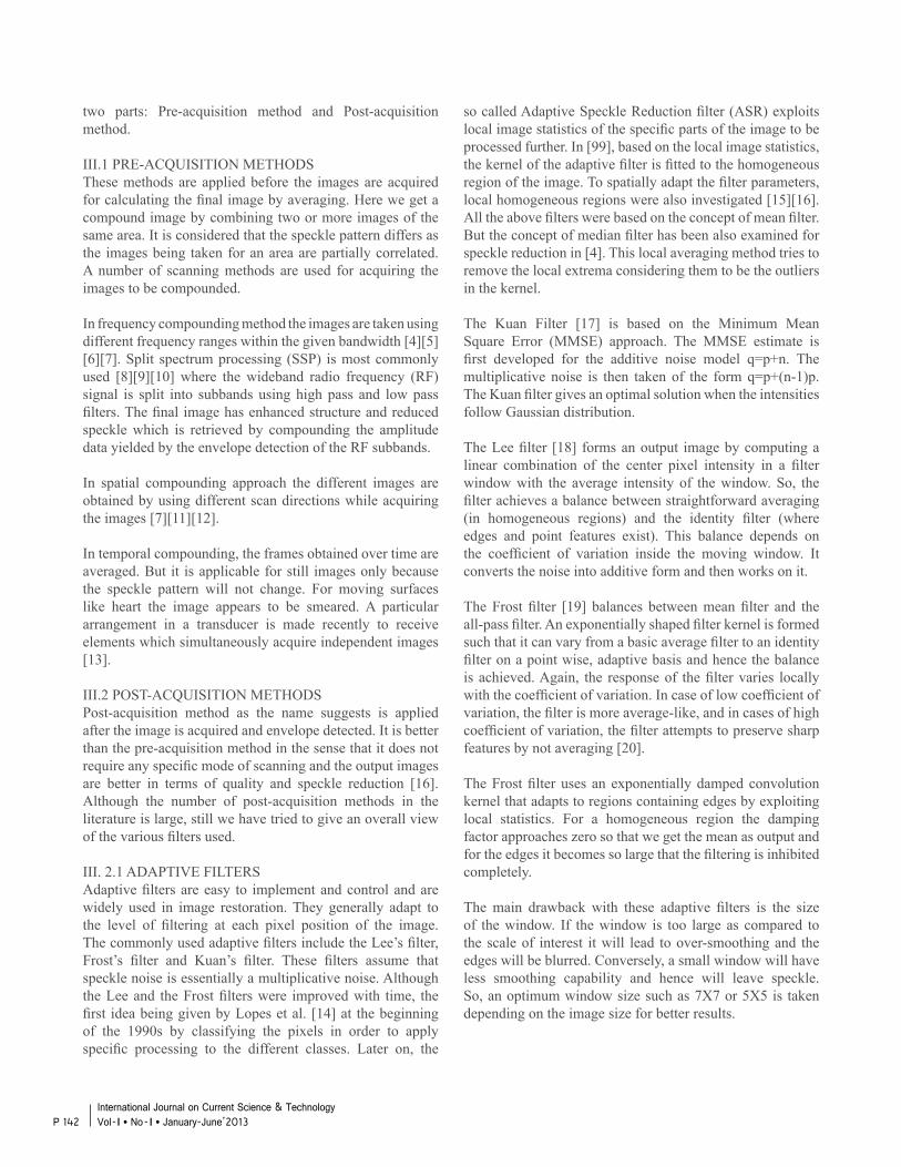
two parts: Pre-acquisition method and Post-acquisition method.
III.1 PRE-ACQUISITION METHODSThese methods are applied before the images are acquired for calculating the final image by averaging. Here we get a compound image by combining two or more images of the same area. It is considered that the speckle pattern differs as the images being taken for an area are partially correlated. A number of scanning methods are used for acquiring the images to be compounded.
In frequency compounding method the images are taken using different frequency ranges within the given bandwidth [4][5][6][7]. Split spectrum processing (SSP) is most commonly used [8][9][10] where the wideband radio frequency (RF) signal is split into subbands using high pass and low pass filters. The final image has enhanced structure and reduced speckle which is retrieved by compounding the amplitude data yielded by the envelope detection of the RF subbands.
In spatial compounding approach the different images are obtained by using different scan directions while acquiring the images [7][11][12].
In temporal compounding, the frames obtained over time are averaged. But it is applicable for still images only because the speckle pattern will not change. For moving surfaces like heart the image appears to be smeared. A particular arrangement in a transducer is made recently to receive elements which simultaneously acquire independent images [13].
III.2 POST-ACQUISITION METHODSPost-acquisition method as the name suggests is applied after the image is acquired and envelope detected. It is better than the pre-acquisition method in the sense that it does not require any specific mode of scanning and the output images are better in terms of quality and speckle reduction [16]. Although the number of post-acquisition methods in the literature is large, still we have tried to give an overall view of the various filters used.
III. 2.1 ADAPTIVE FILTERSAdaptive filters are easy to implement and control and are widely used in image restoration. They generally adapt to the level of filtering at each pixel position of the image. The commonly used adaptive filters include the Lee’s filter, Frost’s filter and Kuan’s filter. These filters assume that speckle noise is essentially a multiplicative noise. Although the Lee and the Frost filters were improved with time, the first idea being given by Lopes et al. [14] at the beginning of the 1990s by classifying the pixels in order to apply specific processing to the different classes. Later on, the
so called Adaptive Speckle Reduction filter (ASR) exploits local image statistics of the specific parts of the image to be processed further. In [99], based on the local image statistics, the kernel of the adaptive filter is fitted to the homogeneous region of the image. To spatially adapt the filter parameters, local homogeneous regions were also investigated [15][16]. All the above filters were based on the concept of mean filter. But the concept of median filter has been also examined for speckle reduction in [4]. This local averaging method tries to remove the local extrema considering them to be the outliers in the kernel.
The Kuan Filter [17] is based on the Minimum Mean Square Error (MMSE) approach. The MMSE estimate is first developed for the additive noise model q=p+n. The multiplicative noise is then taken of the form q=p+(n-1)p. The Kuan filter gives an optimal solution when the intensities follow Gaussian distribution.
The Lee filter [18] forms an output image by computing a linear combination of the center pixel intensity in a filter window with the average intensity of the window. So, the filter achieves a balance between straightforward averaging (in homogeneous regions) and the identity filter (where edges and point features exist). This balance depends on the coefficient of variation inside the moving window. It converts the noise into additive form and then works on it.
The Frost filter [19] balances between mean filter and the all-pass filter. An exponentially shaped filter kernel is formed such that it can vary from a basic average filter to an identity filter on a point wise, adaptive basis and hence the balance is achieved. Again, the response of the filter varies locally with the coefficient of variation. In case of low coefficient of variation, the filter is more average-like, and in cases of high coefficient of variation, the filter attempts to preserve sharp features by not averaging [20].
The Frost filter uses an exponentially damped convolution kernel that adapts to regions containing edges by exploiting local statistics. For a homogeneous region the damping factor approaches zero so that we get the mean as output and for the edges it becomes so large that the filtering is inhibited completely.
The main drawback with these adaptive filters is the size of the window. If the window is too large as compared to the scale of interest it will lead to over-smoothing and the edges will be blurred. Conversely, a small window will have less smoothing capability and hence will leave speckle. So, an optimum window size such as 7X7 or 5X5 is taken depending on the image size for better results.
P 142International Journal on Current Science & Technology Vol - I l No- I l January-June’2013
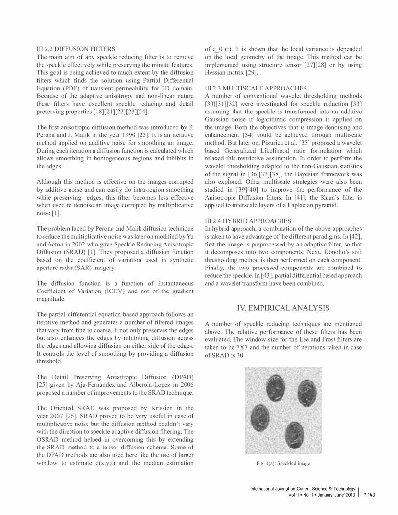
III.2.2 DIFFUSION FILTERSThe main aim of any speckle reducing filter is to remove the speckle effectively while preserving the minute features. This goal is being achieved to much extent by the diffusion filters which finds the solution using Partial Differential Equation (PDE) of transient permeability for 2D domain. Because of the adaptive anisotropy and non-linear nature these filters have excellent speckle reducing and detail preserving properties [18][21][22][23][24].
The first anisotropic diffusion method was introduced by P. Perona and J. Malik in the year 1990 [25]. It is an iterative method applied on additive noise for smoothing an image. During each iteration a diffusion function is calculated which allows smoothing in homogeneous regions and inhibits in the edges.
Although this method is effective on the images corrupted by additive noise and can easily do intra-region smoothing while preserving edges, this filter becomes less effective when used to denoise an image corrupted by multiplicative noise [1].
The problem faced by Perona and Malik diffusion technique to reduce the multiplicative noise was later on modified by Yu and Acton in 2002 who gave Speckle Reducing Anisotropic Diffusion (SRAD) [1]. They proposed a diffusion function based on the coefficient of variation used in synthetic aperture radar (SAR) imagery.
The diffusion function is a function of Instantaneous Coefficient of Variation (ICOV) and not of the gradient magnitude.
The partial differential equation based approach follows an iterative method and generates a number of filtered images that vary from fine to coarse. It not only preserves the edges but also enhances the edges by inhibiting diffusion across the edges and allowing diffusion on either side of the edges. It controls the level of smoothing by providing a diffusion threshold.
The Detail Preserving Anisotropic Diffusion (DPAD) [25] given by Aja-Fernandez and Alberola-Lopez in 2006 proposed a number of improvements to the SRAD technique.
The Oriented SRAD was proposed by Krissien in the year 2007 [26]. SRAD proved to be very useful in case of multiplicative noise but the diffusion method couldn’t vary with the direction to speckle adaptive diffusion filtering. The OSRAD method helped in overcoming this by extending the SRAD method to a tensor diffusion scheme. Some of the DPAD methods are also used here like the use of larger window to estimate q(x,y;t) and the median estimation
of q_0 (t). It is shown that the local variance is depended on the local geometry of the image. This method can be implemented using structure tensor [27][28] or by using Hessian matrix [29].
III.2.3 MULTISCALE APPROACHESA number of conventional wavelet thresholding methods [30][31][32] were investigated for speckle reduction [33] assuming that the speckle is transformed into an additive Gaussian noise if logarithmic compression is applied on the image. Both the objectives that is image denoising and enhancement [34] could be achieved through multiscale method. But later on, Pizurica et al. [35] proposed a wavelet based Generalized Likelihood ratio formulation which relaxed this restrictive assumption. In order to perform the wavelet thresholding adapted to the non-Gaussian statistics of the signal in [36][37][38], the Bayesian framework was also explored. Other multiscale strategies were also been studied in [39][40] to improve the performance of the Anisotropic Diffusion filters. In [41], the Kuan’s filter is applied to interscale layers of a Laplacian pyramid.
III.2.4 HYBRID APPROACHESIn hybrid approach, a combination of the above approaches is taken to have advantage of the different paradigms. In [42], first the image is preprocessed by an adaptive filter, so that it decomposes into two components. Next, Donoho’s soft thresholding method is then performed on each component. Finally, the two processed components are combined to reduce the speckle. In [43], partial differential based approach and a wavelet transform have been combined.
IV. EMPIRICAL ANALYSIS
A number of speckle reducing techniques are mentioned above. The relative performance of these filters has been evaluated. The window size for the Lee and Frost filters are taken to be 7X7 and the number of iterations taken in case of SRAD is 30.
Fig. 1(a): Speckled image
P 143International Journal on Current Science & Technology
Vol - I l No- I l January-June’2013
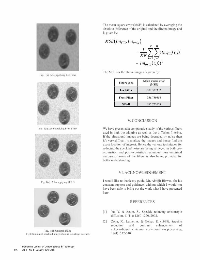
Fig. 1(b): After applying Lee Filter
Fig. 1(c): After applying Frost Filter
Fig. 1(d): After applying SRAD
Fig. 1(e): Original imageFig1: Simulated speckled image of coins (courtesy: internet)
The mean square error (MSE) is calculated by averaging the absolute difference of the original and the filtered image and is given by:
The MSE for the above images is given by:
Filters used Mean square error (MSE)
Lee Filter 907.327332
Frost Filter 356.780853
SRAD 185.725159
V. CONCLUSION
We have presented a comparative study of the various filters used in both the adaptive as well as the diffusion filtering. If the ultrasound images are being degraded by noise then it’s very difficult to analyze the images and hence find the exact location of interest. Hence the various techniques for reducing the speckled noise are being surveyed in both pre-acquisition and post-acquisition techniques. An empirical analysis of some of the filters is also being provided for better understanding.
VI. ACKNOWLEDGEMENT
I would like to thank my guide, Mr. Abhijit Biswas, for his constant support and guidance, without which I would not have been able to bring out the work what I have presented here.
REFERENCES
[1] Yu, Y. & Acton, S., Speckle reducing anisotropic diffusion, 11(11): 1260-1270, 2002.
[2] Zong, X., Laine, A. & Geiser, E. (1998). Speckle reduction and contrast enhancement of echocardiograms via multiscale nonlinear processing, 17(4): 532-540.
P 144International Journal on Current Science & Technology Vol - I l No- I l January-June’2013
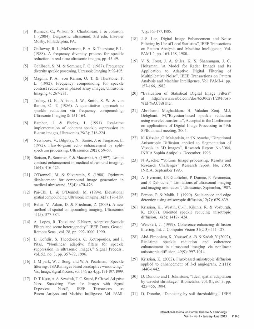
[3] Rumack, C., Wilson, S., Charboneau, J. & Johnson, J. (2004). Diagnostic ultrasound, 3rd edn, Elsevier Mosby, Philadelphia, PA.
[4] Galloway, R. L.,McDermott, B. A. & Thurstone, F. L. (1988). A frequency diversity process for speckle reduction in real-time ultrasonic images, pp. 45-49.
[5] Gehlbach, S. M. & Sommer, F. G. (1987). Frequency diversity speckle processing, Ultrasonic Imaging 9: 92-105.
[6] Magnin, P. A., von Ramm, O. T. & Thurstone, F. L. (1982). Frequency compounding for speckle contrast reduction in phased array images, Ultrasonic Imaging 4: 267-281.
[7] Trahey, G. E., Allison, J. W., Smith, S. W. & von Ramm, O. T. (1986). A quantitative approach to speckle reduction via frequency compounding, Ultrasonic Imaging 8: 151-164.
[8] Bamber, J. & Phelps, J. (1991). Real-time implementation of coherent speckle suppression in B-scan images, Ultrasonics 29(3): 218-224.
[9] Newhouse, V., Bilgutay, N., Saniie, J. & Furgason, E. (1982). Flaw-to-grain echo enhancement by split- spectrum processing, Ultrasonics 20(2): 59-68.
[10] Stetson, P., Sommer, F. & Macovski, A. (1997). Lesion contrast enhancement in medical ultrasound imaging, 16(4): 416-425.
[11] O’Donnell, M. & Silverstein, S. (1988). Optimum displacement for compound image generation in medical ultrasound, 35(4): 470-476.
[12] Pai-Chi, L. & O’Donnell, M. (1994). Elevational spatial compounding, Ultrasonic imaging 16(3): 176-189.
[13] Behar, V., Adam, D. & Friedman, Z. (2003). A new method of spatial compounding imaging, Ultrasonics 41(5): 377-384.
[14] A. Lopes, R. Touzi and E.Nezry, Adaptive Speckle Filters and scene heterogeneity,” IEEE Trans. Geosci. Remote Sens., vol. 28, pp. 992-1000, 1990.
[15] E. Kofidis, S. Theodoridis, C. Kotropoulos, and I. Pitas, “Nonlinear adaptive filters for speckle suppression in ultrasonic images,” Signal Process., vol. 52, no. 3, pp. 357-72, 1996.
[16] J. M park, W. J. Song, and W. A. Pearlman, “Speckle filtering of SAR images based on adaptive windowing,” Vis., Image, Signal Process., vol. 146, no. 4, pp. 191-197, 1999.
[17] D. T. Kuan, A. A. Sawchuk, T. C. Strand, P. Chavel, Adaptive Noise Smoothing Filter for Images with Signal Dependent Noise”, IEEE Transactions on Pattern Analysis and Machine Intelligence, Vol. PAMI-
7, pp. 165-177, 1985.
[18] J.-S. Lee, Digital Image Enhancement and Noise Filtering by Use of Local Statistics”, IEEE Transactions on Pattern Analysis and Machine Intelligence, Vol. PAMI-2, pp. 165-168, 1980.
[19] V. S. Frost, J. A. Stiles, K. S. Shanmugan, J. C. Holtzman, \A Model for Radar Images and Its Application to Adaptive Digital Filtering of Multiplicative Noise”, IEEE Transactions on Pattern Analysis and Machine Intelligence, Vol. PAMI-4, pp. 157-166, 1982.
[20] “Evaluation of Statistical Digital Image Filters” at http://www.scribd.com/doc/65306271/28/Frost- %EF%AC%81lter.
[21] Abrishami Moghaddam. H, Valadan Zouj. M.J, Dehghani. M,”Bayesian-based speckle reduction using wavelet transforms”, Accepted in the Conference on applications of Digital Image Processing in 49th SPIE annual meeting, 2004.
[22] K. Krissian, G. Malandain, and N.Ayache, “Directional Anisotropic Diffusion applied to Segmentation of Vessels in 3D images”, Research Report No.3064, INRIA Sophia Antipolis, December, 1996.
[23] N Ayache. “Volume Image processing, Results and Research Challenges” Research report, No. 2050, INRIA, September 1993.
[24] A- Herment, J.P. Guolielmi, P. Dumee, P. Peronneau, and P. Delouche.,” Limitations of ultrasound imaging and imaging restoration.”, Ultrasonics, September, 1987.
[25] Perona, P. & Malik, J. (1990). Scale-space and edge detection using anisotropic diffusion,12(7): 629-639.
[26] Krissian, K., Westin, C.-F., Kikinis, R. & Vosburgh, K. (2007). Oriented speckle reducing anisotropic diffusion, 16(5): 1412-1424.
[27] Weickert, J. (1999). Coherence-enhancing diffusion filtering, Int. J. Computer Vision 31(2-3): 111-127.
[28] Abd-Elmoniem, K., Youssef, A.-B. & Kadah, Y. (2002), Real-time speckle reduction and coherence enhancement in ultrasound imaging via nonlinear anisotropic diffusion, 49(9): 997-1014.
[29] Krissian, K. (2002). Flux-based anisotropic diffusion applied to enhancement of 3-d angiogram, 21(11): 1440-1442.
[30] D. Donoho and I. Johnstone, “Ideal spatial adaptation by wavelet shrinkage,” Biometrika, vol. 81, no. 3, pp. 425-455, 1994.
[31] D. Donoho, “Denoising by soft-thresholding,” IEEE
P 145International Journal on Current Science & Technology
Vol - I l No- I l January-June’2013
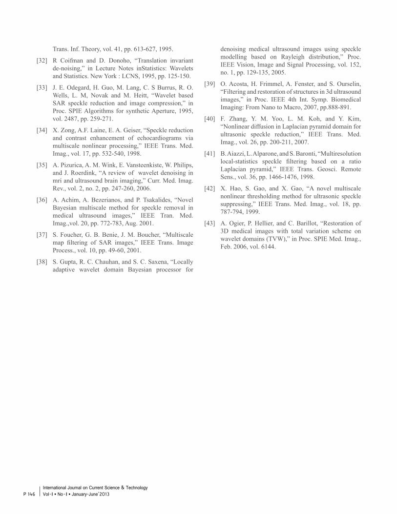
Trans. Inf. Theory, vol. 41, pp. 613-627, 1995.
[32] R Coifman and D. Donoho, “Translation invariant de-noising,” in Lecture Notes inStatistics: Wavelets and Statistics. New York : LCNS, 1995, pp. 125-150.
[33] J. E. Odegard, H. Guo, M. Lang, C. S Burrus, R. O. Wells, L. M, Novak and M. Heitt, “Wavelet based SAR speckle reduction and image compression,” in Proc. SPIE Algorithms for synthetic Aperture, 1995, vol. 2487, pp. 259-271.
[34] X. Zong, A.F. Laine, E. A. Geiser, “Speckle reduction and contrast enhancement of echocardiograms via multiscale nonlinear processing,” IEEE Trans. Med. Imag., vol. 17, pp. 532-540, 1998.
[35] A. Pizurica, A. M. Wink, E. Vansteenkiste, W. Philips, and J. Roerdink, “A review of wavelet denoising in mri and ultrasound brain imaging,” Curr. Med. Imag. Rev., vol. 2, no. 2, pp. 247-260, 2006.
[36] A. Achim, A. Bezerianos, and P. Tsakalides, “Novel Bayesian multiscale method for speckle removal in medical ultrasound images,” IEEE Tran. Med. Imag.,vol. 20, pp. 772-783, Aug. 2001.
[37] S. Foucher, G. B. Benie, J. M. Boucher, “Multiscale map filtering of SAR images,” IEEE Trans. Image Process., vol. 10, pp. 49-60, 2001.
[38] S. Gupta, R. C. Chauhan, and S. C. Saxena, “Locally adaptive wavelet domain Bayesian processor for
denoising medical ultrasound images using speckle modelling based on Rayleigh distribution,” Proc. IEEE Vision, Image and Signal Processing, vol. 152, no. 1, pp. 129-135, 2005.
[39] O. Acosta, H. Frimmel, A. Fenster, and S. Ourselin, “Filtering and restoration of structures in 3d ultrasound images,” in Proc. IEEE 4th Int. Symp. Biomedical Imaging: From Nano to Macro, 2007, pp.888-891.
[40] F. Zhang, Y. M. Yoo, L. M. Koh, and Y. Kim, “Nonlinear diffusion in Laplacian pyramid domain for ultrasonic speckle reduction,” IEEE Trans. Med. Imag., vol. 26, pp. 200-211, 2007.
[41] B. Aiazzi, L. Alparone, and S. Baronti, “Multiresolution local-statistics speckle filtering based on a ratio Laplacian pyramid,” IEEE Trans. Geosci. Remote Sens., vol. 36, pp. 1466-1476, 1998.
[42] X. Hao, S. Gao, and X. Gao, “A novel multiscale nonlinear thresholding method for ultrasonic speckle suppressing,” IEEE Trans. Med. Imag., vol. 18, pp. 787-794, 1999.
[43] A. Ogier, P. Hellier, and C. Barillot, “Restoration of 3D medical images with total variation scheme on wavelet domains (TVW),” in Proc. SPIE Med. Imag., Feb. 2006, vol. 6144.
P 146International Journal on Current Science & Technology Vol - I l No- I l January-June’2013
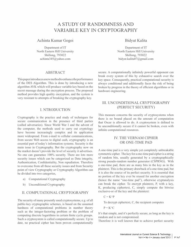
A STUDY OF RANDOMNESS ANDVARIABLE KEY IN CRYPTOGRAPHY
Achinta Kumar Gogoi
Department of IT North Eastern Hill University
Shillong, [email protected]
Bidyut Kalita
Department of IT North Eastern Hill University
Shillong, [email protected]
ABSTRACT
This paper introduces a new method to enhance the performance of the DES Algorithm. This is done by introducing a new algorithm AVK which will produce variable key based on the secret massage during the encryption process. The proposed method provides high quality encryption, and the system is very resistant to attempts of breaking the cryptography key.
I. NTRODUCTION
Cryptography is the practice and study of techniques for secure communication in the presence of third parties (called adversaries). Since World War I and the advent of the computer, the methods used to carry out cryptology have become increasingly complex and its application more widespread. From e-mail to cellular communications, from secure Web access to digital cash, cryptography is an essential part of today’s information systems. Security is the main issue in Cryptography. But the cryptography now on the market doesn’t provide the level of security it advertises. No one can guarantee 100% security. There are lots more security issues which can be categorized as Data integrity, Authentication, Confidentiality, Non repudiation. Therefore to overcome from all these security issues and from Security point of view Cryptography or Cryptography Algorithm can be divided into two categories,
a) Computational Cryptography
b) Unconditional Cryptography
II. COMPUTATIONAL CRYPTOGRAPHY
The security of many presently used cryptosystems, e.g. of all public-key cryptographic schemes, is based on the assumed hardness of computational problems in number theory such as the integer-factoring problem or the problem of computing discrete logarithms in certain finite cycle groups. Such a cryptosystem is called computationally secure. Up to date, no practical cipher has been proven computationally
secure. A computationally infinitely powerful opponent can break every system of this by exhaustive search over the key space. Consequently, practical computational security is always conditional and additionally faces the risk of being broken by progress in the theory of efficient algorithms or in hardware engineering.
III. UNCONDITIONAL CRYPTOGRAPHY (PERFECT SECURITY)
This measure concerns the security of cryptosystems when there is no bound placed on the amount of computation that Oscar is allowed to do. A cryptosystem is defined to be unconditionally secure if it cannot be broken, even with infinite computational resources.
IV. THE VERNAM CIPHEROR ONE-TIME PAD
A one-time pad is a very simple yet completely unbreakable symmetric cipher. The key for a one-time pad cipher is a string of random bits, usually generated by a cryptographically strong pseudo-random number generator (CSPRNG). With a one-time pad, there are as many bits in the key as in the plaintext. This is the primary drawback of a one-time pad, but it is also the source of its perfect security. It is essential that no portion of the key ever be reused for another encryption (hence the name “one-time pad”), otherwise cryptanalysis can break the cipher. To encrypt plaintext, P, with a key, K, producing ciphertext, C, simply compute the bitwise exclusive-or of the key and the plaintext:
C = K^P
To decrypt ciphertext, C, the recipient computes
P = K^C
It’s that simple, and it’s perfectly secure, as long as the key is random and is not compromised. Therefore it is well known that to achieve perfect security
P 147International Journal on Current Science & Technology
Vol - I l No- I l January-June’2013
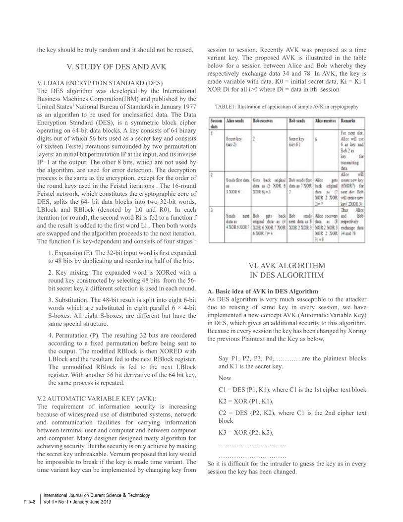
the key should be truly random and it should not be reused.
V. STUDY OF DES AND AVK V.1.DATA ENCRYPTION STANDARD (DES)The DES algorithm was developed by the International Business Machines Corporation(IBM) and published by the United States’ National Bureau of Standards in January 1977 as an algorithm to be used for unclassified data. The Data Encryption Standard (DES), is a symmetric block cipher operating on 64-bit data blocks. A key consists of 64 binary digits out of which 56 bits used as a secret key and consists of sixteen Feistel iterations surrounded by two permutation layers: an initial bit permutation IP at the input, and its inverse IP−1 at the output. The other 8 bits, which are not used by the algorithm, are used for error detection. The decryption process is the same as the encryption, except for the order of the round keys used in the Feistel iterations . The 16-round Feistel network, which constitutes the cryptographic core of DES, splits the 64- bit data blocks into two 32-bit words, LBlock and RBlock (denoted by L0 and R0). In each iteration (or round), the second word Ri is fed to a function f and the result is added to the first word Li . Then both words are swapped and the algorithm proceeds to the next iteration. The function f is key-dependent and consists of four stages :
1. Expansion (E). The 32-bit input word is first expanded to 48 bits by duplicating and reordering half of the bits.
2. Key mixing. The expanded word is XORed with a round key constructed by selecting 48 bits from the 56-bit secret key, a different selection is used in each round.
3. Substitution. The 48-bit result is split into eight 6-bit words which are substituted in eight parallel 6 × 4-bit S-boxes. All eight S-boxes, are different but have the same special structure.
4. Permutation (P). The resulting 32 bits are reordered according to a fixed permutation before being sent to the output. The modified RBlock is then XORED with LBlock and the resultant fed to the next RBlock register. The unmodified RBlock is fed to the next LBlock register. With another 56 bit derivative of the 64 bit key, the same process is repeated.
V.2 AUTOMATIC VARIABLE KEY (AVK):The requirement of information security is increasing because of widespread use of distributed systems, network and communication facilities for carrying information between terminal user and computer and between computer and computer. Many designer designed many algorithm for achieving security. But the security is only achieve by making the secret key unbreakable. Vernum proposed that key would be impossible to break if the key is made time variant. The time variant key can be implemented by changing key from
session to session. Recently AVK was proposed as a time variant key. The proposed AVK is illustrated in the table below for a session between Alice and Bob whereby they respectively exchange data 34 and 78. In AVK, the key is made variable with data. K0 = initial secret data, Ki = Ki-1 XOR Di for all i>0 where Di = data in ith session
TABLE1: Illustration of application of simple AVK in cryptography
VI. AVK ALGORITHMIN DES ALGORITHM
A. Basic idea of AVK in DES AlgorithmAs DES algorithm is very much susceptible to the attacker due to reusing of same key in every session, we have implemented a new concept AVK (Automatic Variable Key) in DES, which gives an additional security to this algorithm. Because in every session the key has been changed by Xoring the previous Plaintext and the Key as below,
Say P1, P2, P3, P4,………….are the plaintext blocks and K1 is the secret key.
Now
C1 = DES (P1, K1), where C1 is the 1st cipher text block
K2 = XOR (P1, K1),
C2 = DES (P2, K2), where C1 is the 2nd cipher text block
K3 = XOR (P2, K2),
………………………….
………………………….So it is difficult for the intruder to guess the key as in every session the key has been changed.
P 148International Journal on Current Science & Technology Vol - I l No- I l January-June’2013
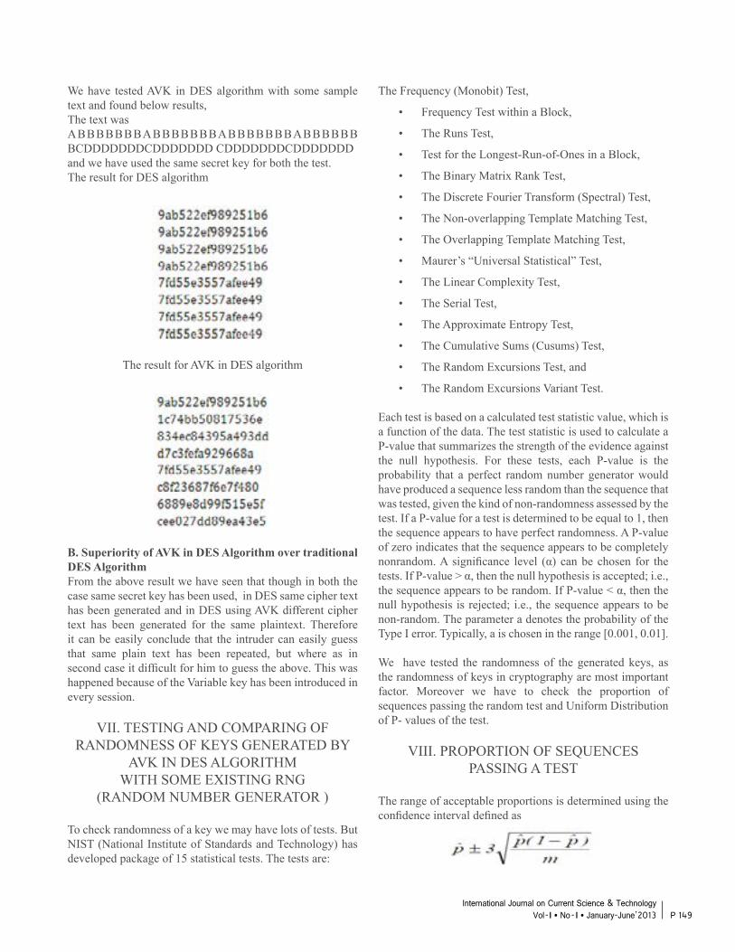
We have tested AVK in DES algorithm with some sample text and found below results,The text was ABBBBBBBABBBBBBBABBBBBBBABBBBBB BCDDDDDDDCDDDDDDD CDDDDDDDCDDDDDDDand we have used the same secret key for both the test.The result for DES algorithm
The result for AVK in DES algorithm
B. Superiority of AVK in DES Algorithm over traditional DES AlgorithmFrom the above result we have seen that though in both the case same secret key has been used, in DES same cipher text has been generated and in DES using AVK different cipher text has been generated for the same plaintext. Therefore it can be easily conclude that the intruder can easily guess that same plain text has been repeated, but where as in second case it difficult for him to guess the above. This was happened because of the Variable key has been introduced in every session.
VII. TESTING AND COMPARING OF RANDOMNESS OF KEYS GENERATED BY
AVK IN DES ALGORITHMWITH SOME EXISTING RNG
(RANDOM NUMBER GENERATOR )
To check randomness of a key we may have lots of tests. But NIST (National Institute of Standards and Technology) has developed package of 15 statistical tests. The tests are:
The Frequency (Monobit) Test,
• Frequency Test within a Block,
• The Runs Test,
• Test for the Longest-Run-of-Ones in a Block,
• The Binary Matrix Rank Test,
• The Discrete Fourier Transform (Spectral) Test,
• The Non-overlapping Template Matching Test,
• The Overlapping Template Matching Test,
• Maurer’s “Universal Statistical” Test,
• The Linear Complexity Test,
• The Serial Test,
• The Approximate Entropy Test,
• The Cumulative Sums (Cusums) Test,
• The Random Excursions Test, and
• The Random Excursions Variant Test.
Each test is based on a calculated test statistic value, which is a function of the data. The test statistic is used to calculate a P-value that summarizes the strength of the evidence against the null hypothesis. For these tests, each P-value is the probability that a perfect random number generator would have produced a sequence less random than the sequence that was tested, given the kind of non-randomness assessed by the test. If a P-value for a test is determined to be equal to 1, then the sequence appears to have perfect randomness. A P-value of zero indicates that the sequence appears to be completely nonrandom. A significance level (α) can be chosen for the tests. If P-value > α, then the null hypothesis is accepted; i.e., the sequence appears to be random. If P-value < α, then the null hypothesis is rejected; i.e., the sequence appears to be non-random. The parameter a denotes the probability of the Type I error. Typically, a is chosen in the range [0.001, 0.01].
We have tested the randomness of the generated keys, as the randomness of keys in cryptography are most important factor. Moreover we have to check the proportion of sequences passing the random test and Uniform Distribution of P- values of the test.
VIII. PROPORTION OF SEQUENCES PASSING A TEST
The range of acceptable proportions is determined using the confidence interval defined as
P 149International Journal on Current Science & Technology
Vol - I l No- I l January-June’2013
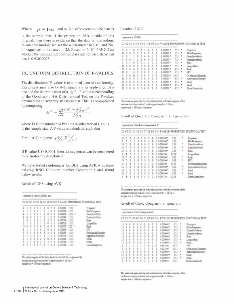
Results of XOR
Result of Quadratic Congruential 1 generator
Result of Cubic Congruential generator
Where and m (No. of sequences to be tested)
is the sample size. If the proportion falls outside of this interval, then there is evidence that the data is nonrandom. In our test module we set the α parameter to 0.01 and No. of sequences to be tested is 25. Based on NIST PRNG Test Module the minimum proportion pass rate for each statistical test is 0.93030075.
IX. UNIFORM DISTRIBUTION OF P-VALUES
The distribution of P-values is examined to ensure uniformity. Uniformity may also be determined via an application of a test and the determination of a P-value corresponding to the Goodness-of-Fit Distributional Test on the P-values obtained for an arbitrary statistical test. This is accomplished by computing
where Fi is the number of Pvalues in sub-interval i, and s is the sample size. A P-value is calculated such that
P-value(U) = igamc
If P-value(U)≥ 0.0001, then the sequences can be considered to be uniformly distributed.
We have tested randomness for DES using AVK with some existing RNG (Random number Generator ) and found below results
Result of DES using AVK
P 150International Journal on Current Science & Technology Vol - I l No- I l January-June’2013
From the above result we can see that AVK in DES has given good result compared to some existing RNG.
X. CONCLUSIONS
DES is now considered to be insecure for many applications. This is chiefly due to the 56-bit key size being too small; in January, 1999, distributed.net and the Electronic Frontier Foundation collaborated to publicly break a DES key in 22 hours and 15 minutes There are also some analytical results which demonstrate theoretical weaknesses in the cipher, although they are unfeasible to mount in practice. So it becomes very important to augment this algorithm by adding new levels of security to make it applicable and can be depending on in any common communication channel. As Shannon proposed the variant key for unconditional or perfect cryptosystem, so application of AVK in DES also follow the concept of variant key which will change session to session. More ever the random keys generated by AVK in DES has passed the randomness tests and giving us good random keys. This will increase the level of security of DES algorithm.
P 151International Journal on Current Science & Technology
Vol - I l No- I l January-June’2013
REFERENCES
[1] “A novel approach towards realizing optimum data transfer and Automatic Variable Key(AVK) in cryptography”, 2008 by P. Chakrabarti, B Bhuyan, A.Chowdhuri, C.T.Bhunia .
[2] P.Chakrabarti, B.Bhuyan, A.Chowdhuri, C.T.Bhunia, “Application of Automatic Variable Key (AVK) in RSA”, accepted for publication in Int’l Journal HIT Transactions on ECCN, Vol 2, No.5 (in press)
[3] P.Chakrabarti , G.H.Mondal , B.Bhuyan ,A.Chowdhuri, C.T.Bhunia “Various New and Modified Approaches for selective encryption with AVK ( diffusion and fuzzy) and their comparative study”, selected and to be published in IEEE Conference, ITNG08, USA, April’08
[4] “A Comparison of Four Pseudo Random Number Generators Implemented in Ada*” by William N. Graham
[5] “New Approach for Modifying Blowfish Algorithm by Using Multiple Keys” by Afaf M. Ali Al-Neaimi†, Rehab F. Hassan

P 152International Journal on Current Science & Technology Vol - I l No- I l January-June’2013
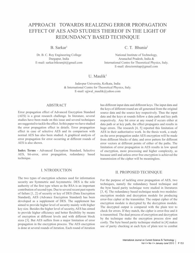
APPROACH TOWARDS REALIZING ERROR PROPAGATION EFFECT OF AES AND STUDIES THEREOF IN THE LIGHT OF
REDUNDANCY BASED TECHNIQUE
C. T. Bhunia2
National Institute of Technology,Arunachal Pradesh, India &
International Centre for Theoretical Physics, Italy.E-mail: [email protected]
U. Maulik3
Jadavpur University, Kolkata, India& International Centre for Theoretical Physics, Italy.
E-mail: [email protected]
B. Sarkar1
Dr. B. C. Roy Engineering CollegeDurgapur, India
E-mail: [email protected]
ABSTRACT
Error propagation effect of Advanced Encryption Standard (AES) is a great research challenge. In literature, several studies have been made on this issue and several techniques are suggested to tackle the effect. In this paper we have studied the error propagation effect in details. Error propagation effect in case of selective AES and its comparison with normal AES has also been studied. A graphical analysis of error propagation for error occurring at different rounds of AES is also shown.
Index Terms - Advanced Encryption Standard, Selective AES, bit-error, error propagation, redundancy based technique.
I. NTRODUCTION
The two types of encryption schemes used for information security are Symmetric and Asymmetric. DES is the sole authority of the first type where as the RSA is an important contribution of second type. Due to several recent past reports of failure [1, 2] of security or key of DES (Data Encryption Standard), AES (Advance Encryption Standard) has been developed as a supplement of DES. The supplement has aimed to provide higher level of security mainly with higher key size. Besides the higher level of security, AES has aimed to provide higher efficiency and better flexibility by means of encryption at different levels and with different block sizes [3]. But AES suffers from a major limitation of error propagation in the encryption process. The AES encryption is done at several rounds of iteration. Each round of iteration
has different input data and different keys. The input data and the keys of different round are all generated from the original source data and the source key respectively. Thus the input data and the keys at rounds follow a data path and key path respectively. Any bit error at any round if occurs either at data path or at key path, the effect propagates and results in huge errors. The research [4, 5] reported this limitation of AES in their authoritative work. In the thesis work, a study on the error propagation under AES encryption will be made from different blocks of data; and error pattern for different error vectors at different points of either of the paths. The limitation of error propagation in AES results in low speed of encryption, more processing and higher complexity, as because until and unless error free encryption is achieved the transmission of the cipher will be meaningless.
II. PROPOSED TECHNIQUE
For the purpose of tackling error propagation of AES, two techniques, namely the redundancy based technique and the byte based parity technique were studied in literatures [3, 4]. The redundancy based technique needs two modules: encryption module and decryption module for producing error-free cipher at the transmitter. The output cipher of the encryption module is decrypted by the decryption module. The decrypted output is compared with the plain text to check for errors. If they match, the cipher is error-free and it is transmitted. The dual process of encryption and decryption by the technique make the encryption process slow and costly. The byte based parity technique studied in [4] makes use of parity checking at each byte of plain text to combat
P 153International Journal on Current Science & Technology
Vol - I l No- I l January-June’2013
error. It is mainly suitable for hardware implementation whereas the redundancy based technique is applicable to both hardware and software based implementations. The redundancy based technique guarantees the error detection / correction for all error vectors that may generate in the AES encryption process where as byte based parity technique does not guarantee the same.
The selective encryption provides a number of advantages in information transportation. In this technique, only a fraction of the entire message is encrypted. As a consequence, the processing time as well as complexity gets reduced. In this literature, we have investigated the application of Selective AES Encryption in redundancy based technique (Fig. 1).
Fig. 1. Selective AES applied in Redundancy Based Technique
III. EXPERIMENTAL RESULTS
We conduct an experiment with plain text message as “ERROR PROPAGATION EFFECT OF AES HAS THROWN A GREAT RESEARCH CHALLENGE BEFORE US.” which is of 640 bits. We will now apply Selective AES for the redundancy based technique. Our observation will be on the selection of S% of blocks from the entire message where the value of S will be taken as 20, 40, 60, 80 and 100. First we divide the entire message into 5 blocks B1, B2, B3, B4 and B5, each of which is of 128 bits, where B1 is “ERROR PROPAGATIO”, B2 is “N EFFECT OF AES ”, B3 is “HAS THROWN A GRE”, B4 is “AT RESEARCH CHAL” and B5 is “LENGE BEFORE US.”
Let us now take the 128-bit key K as “BIKRAMJIT SARKAR”. If we encrypt (AES) the blocks using the key K, say, we get the Cipher Blocks like C1, C2, C3, C4 and C5. So, we can express the Cipher Blocks as follows:
Cn = AES_Encryption (Bn, K), where n ranges from 1 to 5.
Let us assume that the corresponding Hexadecimal values for Bn are HBn, where the values of HBn are as follows:HB1 = 45 52 52 4F 52 20 50 524F 50 41 47 41 54 49 4F
HB2 =4E 20 45 46 46 45 43 5420 4F 46 20 41 45 53 20
HB3 =48 41 53 20 54 48 52 4F57 4E 20 41 20 47 52 45
HB4 =41 54 20 52 45 53 45 4152 43 48 20 43 48 41 4C
HB5 =4C 45 4E 47 45 20 42 4546 4F 52 45 20 55 53 2E
Let us assume that the hexadecimal values for the key K is HK where
HK =42 49 4B 52 41 4D 4A 4954 20 53 41 52 4B 41 52
After the encryption (AES) of Bn using K, we get Cn, where n ranges from 1 to 5. If we consider the corresponding hexadecimal values for Cn to be HCn, we get the hexadecimal values as follows:
HC1 =C4 DA E4 77 D4 07 E6 23FC CB B9 2E 90 BB 8C BE
HC2 =4F 2E 1A 40 55 F2 41 D835 9A 92 72 EB 4C C0 8D
HC3 =68 C8 D3 83 C8 6D 76 FAB0 5C 99 75 8E 1E 19 88
HC4 =4A 4F C4 FF C9 03 56 51BE CB E4 77 73 92 54 59
HC5 =38 6A 56 14 2C F9 DC 495F 1B 66 A1 60 7B A5 C6
The AES Encryption process has 10 rounds. And after each round (1st to 9th) one intermediate state is found and after
P 154International Journal on Current Science & Technology Vol - I l No- I l January-June’2013
the 10 rounds the final cipher text is generated. So, each block Bn, while being encrypted to generate Cn, generates 9 intermediate states. Now say, after first round, the eighth bit of each intermediate state generated from each block HBn get erroneous and consequently we get HCn’ instead of HCn. That means, each (0,0)th cell of the 2D matrices, generated after the completion of the first round of AES algorithm, get somehow changed. Below is the result of forcibly injecting a one-bit error in the eighth bit of the intermediate states during the encryption process after the first round is completed and consequently the generation of faulty cipher text HCn’ instead of what is expected to be.
HC1’ =6F BB 3B B0 82 61 58 C8D7 8F 57 BD 85 DF C9 DC
HC2’ =E8 C9 06 11 93 6F 8C 0013 EA 2E 48 62 1B 8C EB
HC3’ =38 0C 6F 6F 20 DF 9C A033 79 13 69 33 94 CC F4
HC4’ =05 06 41 39 A0 26 34 ECB2 F1 40 46 E0 57 0C E9
HC5’ =D2 0B 43 F7 1A 32 99 A008 F2 41 BD 1C 5A AD 64
Similarly, after fifth round, if the eighth bit of each intermediate state generated from each block HBn gets erroneous, we get HCn” instead of HCn. Below are the faulty ciphers HCn”.
HC1” =F4 E1 51 E0 BA 94 8E AD8F 36 1B 4F B2 52 DA 84
HC2” =93 97 92 5D 9A 13 11 2065 26 A7 71 C4 52 1C 89
HC3” =CC 3E 27 6E 89 D2 A2 F5F6 2D DC 67 5A FD C7 AC
HC4” =42 33 C3 F1 4D 2C 0D 6B
33 DC D8 5A EC 45 B9 7C
HC5” =4B 59 CB D9 1D 29 41 7552 79 B9 2D C8 83 59 AD
Now say, after ninth round, if the eighth bit of each intermediate state generated from each block HBn gets erroneous, we get HCn”’ instead of HCn. Below are the faulty ciphers HCn”’. Below are the faulty ciphers HCn”.
HC1”’ =62 DA E4 77 D4 07 E6 23FC CB B9 2E 90 BB 8C BE
HC2”’ =44 2E 1A 40 55 F2 41 D835 9A 92 72 EB 4C C0 8D
HC3”’ =15 C8 D3 83 C8 6D 76 FAB0 5C 99 75 8E 1E 19 88
HC4”’ =96 4F C4 FF C9 03 56 51BE CB E4 77 73 92 54 59
HC5”’ =51 6A 56 14 2C F9 DC 495F 1B 66 A1 60 7B A5 C6
Now we will compare HCn’, HCn” and HCn”’ with HCn and accordingly we will find the total number of errors at the output ciphers for each of the cases. We will then find the average number of errors occurred in the output cipher when a single bit error has occurred in any of the intermediate states generated during the encryption process.
Comparison in Block B1:
Comparison of HC1’ with HC1: Number of errors is 68.
Comparison of HC1” with HC1: Number of errors is 66.
Comparison of HC1”’ with HC1: Number of errors is 3.
So, the average number of errors occurred is 45.67.
Comparison in Block B2:Comparison of HC2’ with HC2: Number of errors is 65.Comparison of HC2” with HC2: Number of errors is 61.Comparison of HC2”’ with HC2: Number of errors is 3.So, the average number of errors occurred is 43.
P 155International Journal on Current Science & Technology
Vol - I l No- I l January-June’2013
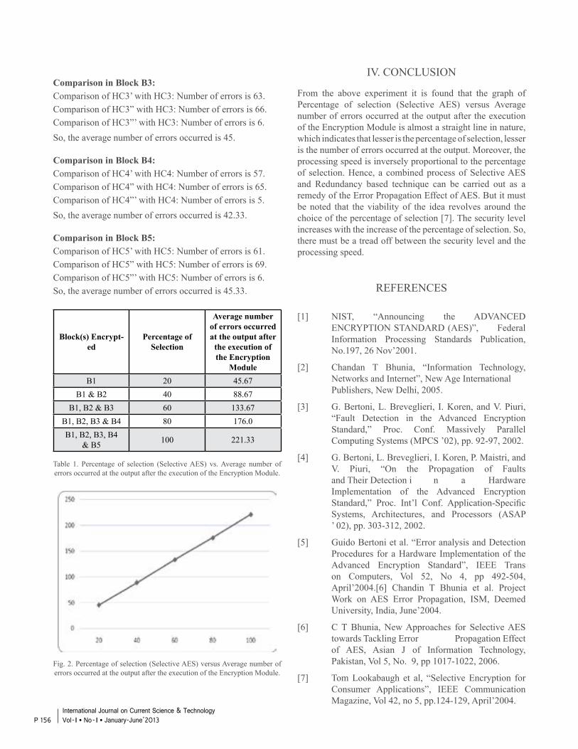
Comparison in Block B3:Comparison of HC3’ with HC3: Number of errors is 63.Comparison of HC3” with HC3: Number of errors is 66.Comparison of HC3”’ with HC3: Number of errors is 6.So, the average number of errors occurred is 45.
Comparison in Block B4:Comparison of HC4’ with HC4: Number of errors is 57.Comparison of HC4” with HC4: Number of errors is 65.Comparison of HC4”’ with HC4: Number of errors is 5.So, the average number of errors occurred is 42.33.
Comparison in Block B5:Comparison of HC5’ with HC5: Number of errors is 61.Comparison of HC5” with HC5: Number of errors is 69.Comparison of HC5”’ with HC5: Number of errors is 6.So, the average number of errors occurred is 45.33.
Block(s) Encrypt-ed
Percentage of Selection
Average number of errors occurred at the output after
the execution of the Encryption
ModuleB1 20 45.67
B1 & B2 40 88.67B1, B2 & B3 60 133.67
B1, B2, B3 & B4 80 176.0B1, B2, B3, B4
& B5 100 221.33
Table 1. Percentage of selection (Selective AES) vs. Average number of errors occurred at the output after the execution of the Encryption Module.
Fig. 2. Percentage of selection (Selective AES) versus Average number of errors occurred at the output after the execution of the Encryption Module.
IV. CONCLUSION
From the above experiment it is found that the graph of Percentage of selection (Selective AES) versus Average number of errors occurred at the output after the execution of the Encryption Module is almost a straight line in nature, which indicates that lesser is the percentage of selection, lesser is the number of errors occurred at the output. Moreover, the processing speed is inversely proportional to the percentage of selection. Hence, a combined process of Selective AES and Redundancy based technique can be carried out as a remedy of the Error Propagation Effect of AES. But it must be noted that the viability of the idea revolves around the choice of the percentage of selection [7]. The security level increases with the increase of the percentage of selection. So, there must be a tread off between the security level and the processing speed.
REFERENCES
[1] NIST, “Announcing the ADVANCED ENCRYPTION STANDARD (AES)”, Federal Information Processing Standards Publication, No.197, 26 Nov’2001.
[2] Chandan T Bhunia, “Information Technology, Networks and Internet”, New Age International Publishers, New Delhi, 2005.
[3] G. Bertoni, L. Breveglieri, I. Koren, and V. Piuri, “Fault Detection in the Advanced Encryption Standard,” Proc. Conf. Massively Parallel Computing Systems (MPCS ’02), pp. 92-97, 2002.
[4] G. Bertoni, L. Breveglieri, I. Koren, P. Maistri, and V. Piuri, “On the Propagation of Faults and Their Detection i n a Hardware Implementation of the Advanced Encryption Standard,” Proc. Int’l Conf. Application-Specific Systems, Architectures, and Processors (ASAP ’ 02), pp. 303-312, 2002.
[5] Guido Bertoni et al. “Error analysis and Detection Procedures for a Hardware Implementation of the Advanced Encryption Standard”, IEEE Trans on Computers, Vol 52, No 4, pp 492-504, April’2004.[6] Chandin T Bhunia et al. Project Work on AES Error Propagation, ISM, Deemed University, India, June’2004.
[6] C T Bhunia, New Approaches for Selective AES towards Tackling Error Propagation Effect of AES, Asian J of Information Technology, Pakistan, Vol 5, No. 9, pp 1017-1022, 2006.
[7] Tom Lookabaugh et al, “Selective Encryption for Consumer Applications”, IEEE Communication Magazine, Vol 42, no 5, pp.124-129, April’2004.
P 156International Journal on Current Science & Technology Vol - I l No- I l January-June’2013

[8] B Sarkar et al., Study and Analysis of Error Propagation Effect of Advanced Encryption Standard”, Int’l J HIT Transaction on ECCN, Vol. - 2, No. - 7, 2008.
[9] B. Sarkar et al., “Modified Redundancy based
P 157International Journal on Current Science & Technology
Vol - I l No- I l January-June’2013
Technique - a New Approach to Combat Error Propagation Effect of AES”, Springer Journal of Institution of Engineers Series B, DOI: 10.1007/ s40031-012-0012-1.

P 158International Journal on Current Science & Technology Vol - I l No- I l January-June’2013
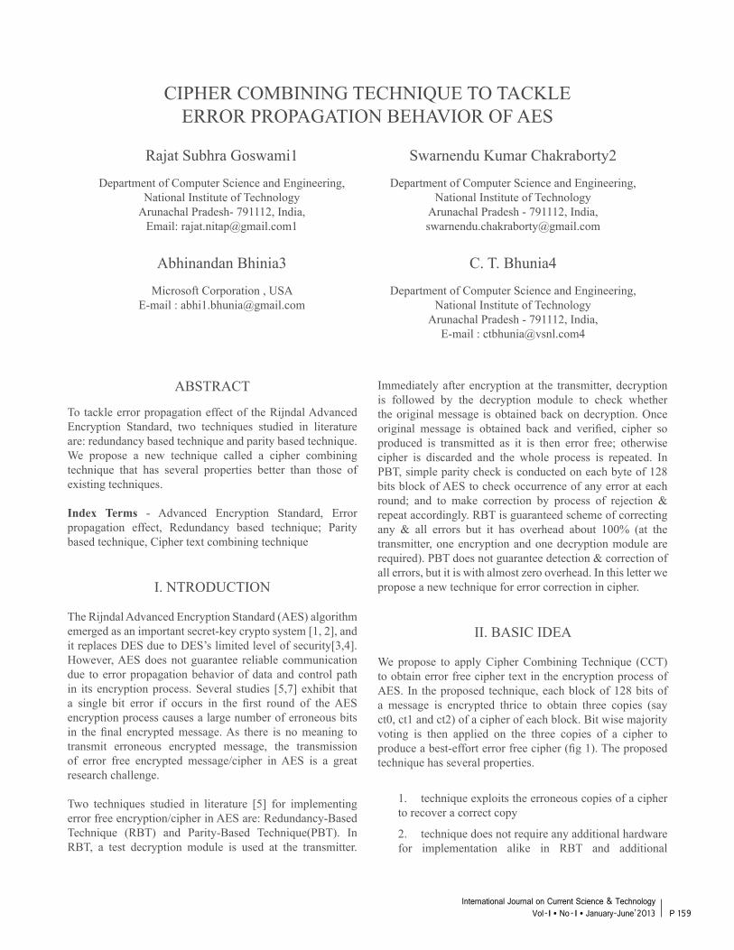
CIPHER COMBINING TECHNIQUE TO TACKLEERROR PROPAGATION BEHAVIOR OF AES
Rajat Subhra Goswami1
Department of Computer Science and Engineering, National Institute of Technology
Arunachal Pradesh- 791112, India, Email: [email protected]
Abhinandan Bhinia3
Microsoft Corporation , USA E-mail : [email protected]
Swarnendu Kumar Chakraborty2
Department of Computer Science and Engineering, National Institute of Technology
Arunachal Pradesh - 791112, India, [email protected]
C. T. Bhunia4
Department of Computer Science and Engineering, National Institute of Technology
Arunachal Pradesh - 791112, India, E-mail : [email protected]
ABSTRACT
To tackle error propagation effect of the Rijndal Advanced Encryption Standard, two techniques studied in literature are: redundancy based technique and parity based technique. We propose a new technique called a cipher combining technique that has several properties better than those of existing techniques.
Index Terms - Advanced Encryption Standard, Error propagation effect, Redundancy based technique; Parity based technique, Cipher text combining technique
I. NTRODUCTION
The Rijndal Advanced Encryption Standard (AES) algorithm emerged as an important secret-key crypto system [1, 2], and it replaces DES due to DES’s limited level of security[3,4]. However, AES does not guarantee reliable communication due to error propagation behavior of data and control path in its encryption process. Several studies [5,7] exhibit that a single bit error if occurs in the first round of the AES encryption process causes a large number of erroneous bits in the final encrypted message. As there is no meaning to transmit erroneous encrypted message, the transmission of error free encrypted message/cipher in AES is a great research challenge.
Two techniques studied in literature [5] for implementing error free encryption/cipher in AES are: Redundancy-Based Technique (RBT) and Parity-Based Technique(PBT). In RBT, a test decryption module is used at the transmitter.
Immediately after encryption at the transmitter, decryption is followed by the decryption module to check whether the original message is obtained back on decryption. Once original message is obtained back and verified, cipher so produced is transmitted as it is then error free; otherwise cipher is discarded and the whole process is repeated. In PBT, simple parity check is conducted on each byte of 128 bits block of AES to check occurrence of any error at each round; and to make correction by process of rejection & repeat accordingly. RBT is guaranteed scheme of correcting any & all errors but it has overhead about 100% (at the transmitter, one encryption and one decryption module are required). PBT does not guarantee detection & correction of all errors, but it is with almost zero overhead. In this letter we propose a new technique for error correction in cipher.
II. BASIC IDEA
We propose to apply Cipher Combining Technique (CCT) to obtain error free cipher text in the encryption process of AES. In the proposed technique, each block of 128 bits of a message is encrypted thrice to obtain three copies (say ct0, ct1 and ct2) of a cipher of each block. Bit wise majority voting is then applied on the three copies of a cipher to produce a best-effort error free cipher (fig 1). The proposed technique has several properties.
1. technique exploits the erroneous copies of a cipher to recover a correct copy
2. technique does not require any additional hardware for implementation alike in RBT and additional
P 159International Journal on Current Science & Technology
Vol - I l No- I l January-June’2013
processing alike in PBT
3. technique may be easily implemented both in hardware and software
4. however, technique does not guarantee correction of all sorts of error, although such a possibility is rare. If probability of a bit error at a particular location of a cipher is p, the probability of failure in CCT is then p2.
Fig. 1: Illustration of CCT
III. CONCLUSION
We have put forward a basic idea for obtaining error free cipher at transmitter of AES. The idea is decisively to outperform existing techniques. Experimental verification is due.
REFERENCES
[1] C T Bhunia, “IT, Network and Internet,” New Age Publications, New Delhi, 2005
[2] B Gladman, “A Specification for Rijndal, the AES algorithm,” http://fp.gladman.plus.com/2001.
[3] NIST, “Announcing the ADVAN ENCRYPTION STANDARD(AES)”, Federal Information Processing Standards Publication, no 197, 26 Nov, 2001.
[4] M Akkar and C Giraud, “ Implemention of DES and AES, secure against Some Attacks,” Proc. Workshop Cryptographic Hardware and Embedded Systems(CHES’01), pp. 68-80, 2001.
[5] G Bertoni, L Breveglieri et all, “Error Analysis and Detection Procedures for a Hardware Implementation of the Advanced Encryption Standard,”, IEEE Trans. On Computers, Vol 62, No 4, pp.1-14, April, 2003.
[6] B Bhuyan and C T Bhunia, Ph D thesis, “Approaches to Implement Selective Encryption with High Level of Security” Jadavpur University, India, 2010.
P 160International Journal on Current Science & Technology Vol - I l No- I l January-June’2013
TWO NEW PROTOCOLS FOR IMPROVINGPERFORMANCE OF AGGRESSIVE PACKET COMBINING
Swarnendu Kumar Chakraborty1
Department of Computer Science and Engineering, National Institute of Technology
Arunachal Pradesh- 791112, India, Email: [email protected]
Abhinandan Bhinia3
Microsoft Corporation , USA E-mail : [email protected]
Rajat Subhra Goswami2
Department of Computer Science and Engineering, National Institute of Technology
Arunachal Pradesh - 791112, India, E-mail : [email protected]
C. T. Bhunia4
Department of Computer Science and Engineering, National Institute of Technology, Arunachal Pradesh -
791112, India, E-mail : [email protected]
ABSTRACT
In the paper, two protocols are suggested to improve the performance of of aggressive packet combining scheme(APC). To combat error in computer / data communication networks, ARQ (Automatic Repeat Request) techniques are used. Several modifications to improve performance of ARQ are suggested in literature.
The important modifications are majority packet combining scheme (MjPC proposed by Wicker), packet combining scheme (PC proposed by Chakraborty), modified packet combining scheme (MPC proposed by Bhunia), and packet reversed packet combining (PRPC proposed by Bhunia) scheme. These modifications are appropriate for improving throughput of conventional ARQ protocols. Leung proposed an idea of APC for error control in wireless networks with basic objective of error control in uplink wireless data network. We suggest two modifications of APC to improve its performance in terms of higher throughput.
Index Terms - Error control, Aggressive Packet Combining Scheme, Packet Reversed Packet Combining Scheme, Modified packet combining scheme
I. NTRODUCTION
In order to transfer data reliably from source to destination either BEC (Backward Error Control) or FEC (Forward Error Control) strategies are used. It is well established
that BEC strategy is sufficient for wired communication, and FEC strategy is required for wireless transmission. Several research attempted to apply BEC in wireless communication as BEC is cost effective. BEC is implemented by automatic repeat request (ARQ) protocols [1-17] in which the erroneous packet received by the receiver is corrected by the retransmission of a copy of the same packet from transmitter. BEC uses error detection code unlike FEC that is costly as it consumes higher bandwidth for using error correction code. In order to realize the best of all, it is decisively desirable to employ arq in modified form to control error in wireless networks. The bit error rate of wireless channels. is high[18-20] in the range of 10-2 to 10-4. For enabling a reasonable performance radio link bit error rate requires to be within a range of 10-6 to 10-8 [21]. In order to achieve the desirable quality in high bit error rate wireless channels, two important modifications for applying basic ARQ are found in literature: Multiple route packet combining scheme [22] and Aggressive packet combining scheme [23]. APC does not address of improving throughput rather attempts to lower down complexities of handheld device, power consumption and bandwidth utilization in the uplink. We address the issues with two modifications.
Chakraborty [24-26] suggested a very simple and elegant technique, known as packet combining technique, for error correction using BEC strategy. The technique aims to minimize delay in correction process. Several modifications of PC are found in literature, and these are MPC [27], PRPC [28] and Error Forecasting PC [29]. However, we propose to apply these modifications in APC for better performance.
P 161International Journal on Current Science & Technology
Vol - I l No- I l January-June’2013
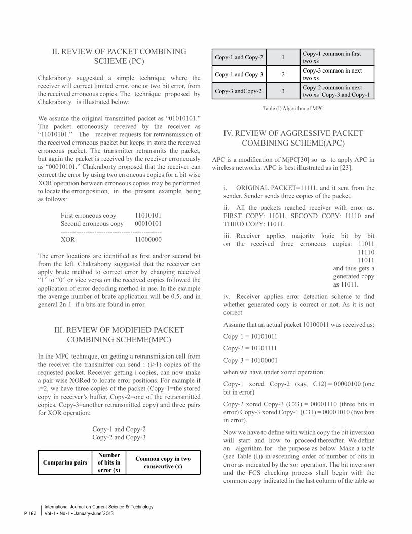
II. REVIEW OF PACKET COMBINING SCHEME (PC)
Chakraborty suggested a simple technique where the receiver will correct limited error, one or two bit error, from the received erroneous copies. The technique proposed by Chakraborty is illustrated below:
We assume the original transmitted packet as “01010101.” The packet erroneously received by the receiver as “11010101.” The receiver requests for retransmission of the received erroneous packet but keeps in store the received erroneous packet. The transmitter retransmits the packet, but again the packet is received by the receiver erroneously as “00010101.” Chakraborty proposed that the receiver can correct the error by using two erroneous copies for a bit wise XOR operation between erroneous copies may be performed to locate the error position, in the present example being as follows:
First erroneous copy 11010101Second erroneous copy 00010101---------------------------------------------XOR 11000000
The error locations are identified as first and/or second bit from the left. Chakraborty suggested that the receiver can apply brute method to correct error by changing received “1” to “0” or vice versa on the received copies followed the application of error decoding method in use. In the example the average number of brute application will be 0.5, and in general 2n-1 if n bits are found in error.
III. REVIEW OF MODIFIED PACKET COMBINING SCHEME(MPC)
In the MPC technique, on getting a retransmission call from the receiver the transmitter can send i (i>1) copies of the requested packet. Receiver getting i copies, can now make a pair-wise XORed to locate error positions. For example if i=2, we have three copies of the packet (Copy-1=the stored copy in receiver’s buffer, Copy-2=one of the retransmitted copies, Copy-3=another retransmitted copy) and three pairs for XOR operation:
Copy-1 and Copy-2Copy-2 and Copy-3
Comparing pairsNumber of bits in error (x)
Common copy in two consecutive (x)
Copy-1 and Copy-2 1 Copy-1 common in first two xs
Copy-1 and Copy-3 2 Copy-3 common in next two xs
Copy-3 andCopy-2 3 Copy-2 common in next two xs Copy-3 and Copy-1
Table (I) Algorithm of MPC
IV. REVIEW OF AGGRESSIVE PACKET COMBINING SCHEME(APC)
APC is a modification of MjPC[30] so as to apply APC in wireless networks. APC is best illustrated as in [23].
i. ORIGINAL PACKET=11111, and it sent from the sender. Sender sends three copies of the packet.
ii. All the packets reached receiver with error as: FIRST COPY: 11011, SECOND COPY: 11110 and THIRD COPY: 11011.
iii. Receiver applies majority logic bit by bit on the received three erroneous copies: 11011 11110 11011 and thus gets a generated copy as 11011.
iv. Receiver applies error detection scheme to find whether generated copy is correct or not. As it is not correct
Assume that an actual packet 10100011 was received as:
Copy-1 = 10101011
Copy-2 = 10101111
Copy-3 = 10100001
when we have under xored operation:
Copy-1 xored Copy-2 (say, C12) = 00000100 (one bit in error)
Copy-2 xored Copy-3 (C23) = 00001110 (three bits in error) Copy-3 xored Copy-1 (C31) = 00001010 (two bits in error).
Now we have to define with which copy the bit inversion will start and how to proceed thereafter. We define an algorithm for the purpose as below. Make a table (see Table (I)) in ascending order of number of bits in error as indicated by the xor operation. The bit inversion and the FCS checking process shall begin with the common copy indicated in the last column of the table so
P 162International Journal on Current Science & Technology Vol - I l No- I l January-June’2013
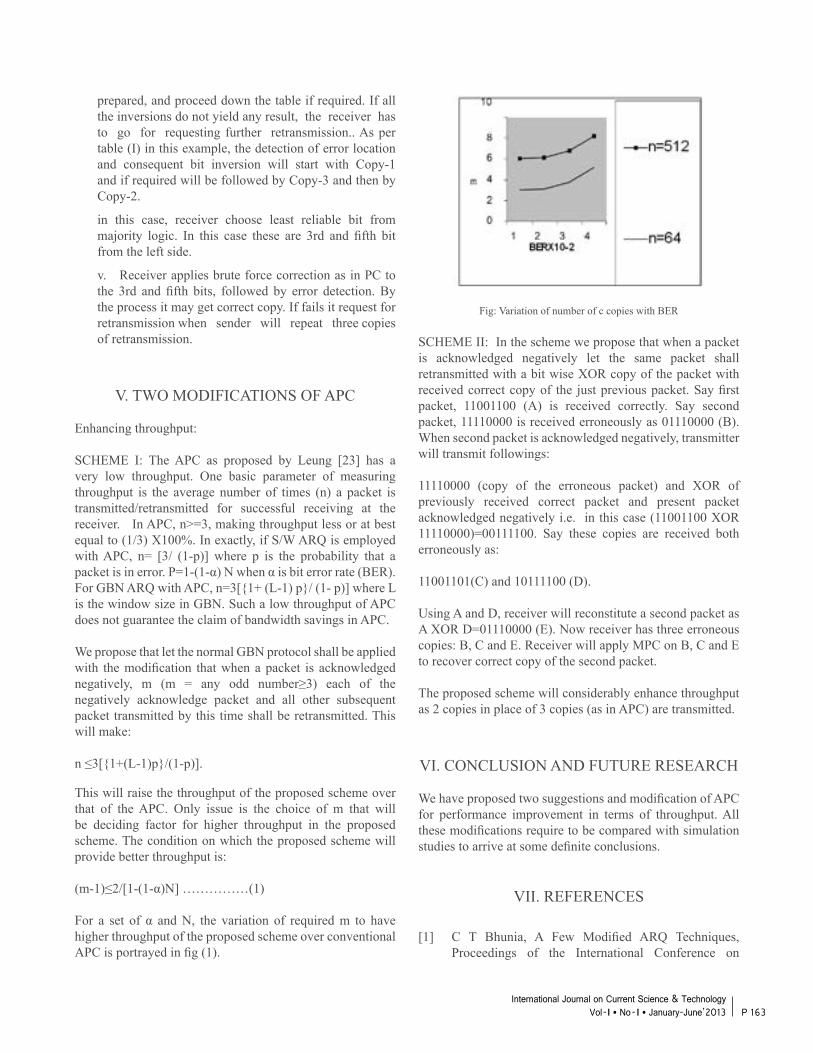
prepared, and proceed down the table if required. If all the inversions do not yield any result, the receiver has to go for requesting further retransmission.. As per table (I) in this example, the detection of error location and consequent bit inversion will start with Copy-1 and if required will be followed by Copy-3 and then by Copy-2.
in this case, receiver choose least reliable bit from majority logic. In this case these are 3rd and fifth bit from the left side.
v. Receiver applies brute force correction as in PC to the 3rd and fifth bits, followed by error detection. By the process it may get correct copy. If fails it request for retransmission when sender will repeat three copies of retransmission.
V. TWO MODIFICATIONS OF APC
Enhancing throughput:
SCHEME I: The APC as proposed by Leung [23] has a very low throughput. One basic parameter of measuring throughput is the average number of times (n) a packet is transmitted/retransmitted for successful receiving at the receiver. In APC, n>=3, making throughput less or at best equal to (1/3) X100%. In exactly, if S/W ARQ is employed with APC, n= [3/ (1-p)] where p is the probability that a packet is in error. P=1-(1-α) N when α is bit error rate (BER). For GBN ARQ with APC, n=3[1+ (L-1) p/ (1- p)] where L is the window size in GBN. Such a low throughput of APC does not guarantee the claim of bandwidth savings in APC.
We propose that let the normal GBN protocol shall be applied with the modification that when a packet is acknowledged negatively, m (m = any odd number≥3) each of the negatively acknowledge packet and all other subsequent packet transmitted by this time shall be retransmitted. This will make:
n ≤3[1+(L-1)p/(1-p)].
This will raise the throughput of the proposed scheme over that of the APC. Only issue is the choice of m that will be deciding factor for higher throughput in the proposed scheme. The condition on which the proposed scheme will provide better throughput is:
(m-1)≤2/[1-(1-α)N] ……………(1)
For a set of α and N, the variation of required m to have higher throughput of the proposed scheme over conventional APC is portrayed in fig (1).
Fig: Variation of number of c copies with BER
SCHEME II: In the scheme we propose that when a packet is acknowledged negatively let the same packet shall retransmitted with a bit wise XOR copy of the packet with received correct copy of the just previous packet. Say first packet, 11001100 (A) is received correctly. Say second packet, 11110000 is received erroneously as 01110000 (B). When second packet is acknowledged negatively, transmitter will transmit followings:
11110000 (copy of the erroneous packet) and XOR of previously received correct packet and present packet acknowledged negatively i.e. in this case (11001100 XOR 11110000)=00111100. Say these copies are received both erroneously as:
11001101(C) and 10111100 (D).
Using A and D, receiver will reconstitute a second packet as A XOR D=01110000 (E). Now receiver has three erroneous copies: B, C and E. Receiver will apply MPC on B, C and E to recover correct copy of the second packet.
The proposed scheme will considerably enhance throughput as 2 copies in place of 3 copies (as in APC) are transmitted.
VI. CONCLUSION AND FUTURE RESEARCH
We have proposed two suggestions and modification of APC for performance improvement in terms of throughput. All these modifications require to be compared with simulation studies to arrive at some definite conclusions.
VII. REFERENCES
[1] C T Bhunia, A Few Modified ARQ Techniques, Proceedings of the International Conference on
P 163International Journal on Current Science & Technology
Vol - I l No- I l January-June’2013
Communications, Computers & Devices, ICCCD-2000, 14-16, Decedmber’2000, I I T, Kharagpur, India, Vol.II, pp. 705-708J. Clerk Maxwell, A Treatise on Electricity and Magnetism, 3rd ed., vol. 2. Oxford: Clarendon, 1892, pp.68-73.
[2] C T Bhunia and A Chowdhury, ARQ Technique with Variable Number of Copies in Retransmission, Proceedings of Conference on Computer Networking and Multimedia (COMNAM-2000), 21-22 December’2000, Javadpur University, Calcutta, India, pp.16-21 .
[3] C T Bhunia and A Chowdhury, Performance Analysis of ARQ Techniques used in Computer Communication Using Delay as a Parameter, Proceedings of Conference on Computer Networking and Multimedia (COMNAM-2000), Jadavpur University, Calcutta, India, pp.22-24.
C T Bhunia, ARQ with two level coding with generalized parity and i (i>1) copies of parts in retransmission, Proceedings of National Conference on Data Communications (NCDC- 2000), Computer Society of India, Chandigarh, India, 7-8 April’2000, pp.19
[4] C T Bhunia, ARQ Techniques: Review and Modifications, Journal IETE Technical Review, Sept- Oct’2001 Vol18, No 5, pp 381-401
[5] R J Beniece and A H Frey Jr, An analysis of retransmission schemes, IEEE Trans Comm Tech, COM-12, pp 135-145, Dec 1964
[6] S Lin, D Costello Jr and M J Miller, Automatic repeat request error control schemes, IEEE Comm Mag, 22, pp 5-17, Dec ‘1984.
[7] A R K Sastry, Improving Automatic Repeat Request (ARQ) Performance on Satellite Channels Under High Error Rate Conditions, IEEE Trans Comm, April’77, pp 436-439.
[8] Joel M Morries, On Another Go-Back -N ARQ Technique For High Error Rate Conditions, IEEE Trans Comm, Vol 26, No 1, Jan’78, pp 186-189.
[9] E J Weldon Jr, An Improved Selective Repeat ARQ Strategy, IEEE Trans Comm, Vol 30, No 3, March’82, pp 480-486.
[10] Don Towsley, The Shutter Go Back-N ARQ Protocol, IEEE Trans Comm, Vol 27, No 6, June’79, pp 869-875.
[11] Dimirti Bertsekas et al, Data Networks, Prentice Hall of India, 1992, Ch-2
[12] G E Keiser, Local Area Networks, McGrawhill, USA, 1995
[13] N D Birrell, Pre-emptive retransmission for
communication over noisy channels, IEE Proc Part F, Vol 128, 1981, pp 393-400.
[14] H Bruneel and M Moeneclacey, On the throughput performance of some continuous ARQ strategies with repeated transmissions, IEEE Trans Comm, Vol COM m34, 1986, pp 244-249.
[15] Y wang and S Lin, A Modified Selective Repeat Type- Ii Hybrid ARQ System and its Performance Analysis, IEEE Trans Comm, Vol Com 31, May’1983, pp. 593-608.
[16] S B Wicker and M J Bartz, Type-II Hybrid ARQ Protocol using Punctured MDS Code, IEEE Trans Comm, Vol 42, Feb-March- April’1994, pp. 1431-1440.
[17] O Yuen, Design trde-offs cellular/PCS systems, IEEE Comm Mag., Vol. 34, No 9, Sept’1996, pp 146-152
[18] H Liu. H Ma, M E Zarki, and S Gupta, Error control schemes for networks: An overview, Mobile Networks and Applications, Vol. 2, 1997, pp 167-182.
[19] A Pahlavan and A H Levesque, Wireless Data Communication, Proc. IEEE, Vol 82, No 9, Sept’1994, pp 1398-1430
[20] Dzmitry Kliazovich, Nadhir Ben Halima and Fabizio Granelli, context-aware receiver - driven retransmission Control in Wireless Local Area Networks, found in Internet.
[21] Y Hirayama, H Okada, T Yamazato and M Katayama, Time-Dependent Analysis of the Multiple-Route Packet Combining Scheme in Wireless Multihop Network, Int J wireless Information Networks, Vol. 42, No 1Jan’2005, pp 35-44.
[22] Yiu-Wing LEUNG, Aggressive Packet Combining for Error Control in Wireless Networks, trans. Comm Vol. E83, No 2Feb’2000, pp38-385
[23] Shyam S. Chakraborty et al, An ARQ Scheme with Packet Combining, IEEE Comm Letters, Vol 2, No 7, July’95, pp 200-202.
[24] Shyam S Chakraborty et al, An Exact Analysis of an Adaptive GBN Scheme with Sliding Observation Interval Mechanism, IEEE Comm Letters, Vol 3, No. 5,May’99, pp 151-153.
[25] Shyam S Chakraborty et al, An Adaptive ARQ Scheme with Packet Combining for Time Varying Channels, IEEE Comm Letters, Vol 3, No 2, Feb’1999, pp 52-54.
[26] C T Bhunia, Modified Packet Combining Scheme using Error Forecasting Decoding to combat error in network, Proc. ICITA’05(Proc. IEEE Computer Soc.), Sydney, Vol, 2, 4-7, July’2005, pp 641-646
[27] C T Bhunia, Packet Reversed Packet Combining
P 164International Journal on Current Science & Technology Vol - I l No- I l January-June’2013
Scheme, Proc. IEEE Computer Soc, CIT’07, Aizu University, Japan, pp. 447-451
[28] C T Bhunia, Error forecasting Schemes of error Correction at Receiver, Proc ITNG’2008, IEEE C o m p u t e r Society , USA , pp . 332 - 336 [30] S B Wicker, Adaptive rate error control through the use of diverse combining and majority logic decoding in hybrid ARQ protocol, IEEE Trans Comm., Vol.39. No. 3, March’1991, pp 380-385.
[29] C T Bhunia, Exact Analyzing Performance of New and Modified GBN scheme for Noisy Wireless Environment, J Inst Engrs, India, Vol.89, Jan’2009, pp 27-31
P 165International Journal on Current Science & Technology
Vol - I l No- I l January-June’2013
[30] C T Bhunia, IT, Network & Internet, New Age International Publishers, India, 2005 [33]Michele Zorzi and Ramesh R Rao, Lateness Probability of a Retransmission Scheme for Error Control on a Two-State Markov Channel, IEEE Transactions on Communications, Vol. 47, No. 10, October’1999, pp.1537-1548.
[31] C T Bhunia et al, Pre Emptive Dynamic Source Routing: A Repaired Back Up Approach and stability Based DSR with Multiple routes, J Comp & Information Tech, CIT, Croatia, Vol.16, No. 2, 2008, pp 91-99.

P 166International Journal on Current Science & Technology Vol - I l No- I l January-June’2013
REVIEW AND SECURITY ANALYSIS OF AN EFFICIENT BIOMETRIC-BASED REMOTE
USER AUTHENTICATION SCHEME USING SMART CARDS
Kiran Sankar Das
M.Tech (CSE)Bengal Institute Of Technology & management
Santiniketan,IndiaE-mail : [email protected]
Uddalak Chatterjee
Department of Computer Science & InformaticsBengal Institute Of Technology & management
Santiniketan,IndiaE-mail : [email protected]
Subhasish Banerjee
Department of Computer Science & InformaticsBengal Institute Of Technology & management
Santiniketan,IndiaE-mail : [email protected]
ABSTRACT
A path braking scheme on biometric-based remote user authentication has been proposed by Li-Hwang In 2010. Later in 2011, A. K. Das showed some shortfalls of the Li-Hwang scheme and proposed an efficient biometric based remote user authentication scheme using smart cards that overcomes the shortfalls of the main Li- Hwang scheme and provides mutual authentication. In this paper, we reviewed and analyzed Das’s scheme and pointed out some existing flaws mainly based on Smart Card tampering and revealing stored information.
I. NTRODUCTION
In the field of recent e-commerce and m-commerce remote user authentication has been a great research domain. However, day-by-day progress in technology and network access methods exposed serious security weaknesses in remote user authentication process due to week password management and advanced attack techniques. several schemes [1-6] have shown various ways to tamper user authentication and get access unethically to various authentication processes.
In traditional systems of identity-based user recognition remote user authentication was based on password. But passwords can be guessed easily with some basic dictionary attacks. Later to overcome these problems passwords were encrypted with cryptographic secret keys. But the long cryptographic keys were difficult to memories and moreover they are lost, forgotten and easily shared therefore unable to
provide non-repudiation. In a client- server systems password based authentication with smartcard are proposed in [7-8].
A biometric system is basically a pattern recognition system which extracts some pattern set from user’s provided biometry and acquires a feature set and further verifies it with the stored template set in systems database. [9-11]. In recent work [12-14], biometric based remote user authentication schemes shown strong authentication protections against Password theft and fake user attacks. Some advantageous features of biometric keys are as follows-
• Biometric keys cannot be lost or forgotten.
• Biometric keys are very difficult to share or copy.
• Biometric keys are extremely hard to forge or distribute.
• Biometric keys cannot be guessed.
• Someone’s biometrics is not easy to break with others.
Therefore biometric key based authentication is more secure and reliable than traditional password based authentication schemes.
Therefore biometric key based authentication is more secure and reliable than traditional password based authentication schemes. In this report we analyzed Das’s scheme and shown that Das’s authentication scheme is still vulnerable to various attacks and does not provide mutual authentication between the user and the server. In [16-17] researches revealed that
P 167International Journal on Current Science & Technology
Vol - I l No- I l January-June’2013
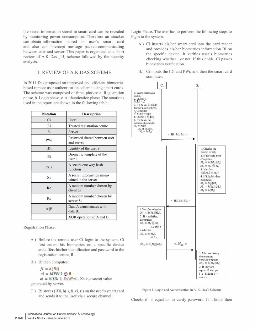
the secret information stored in smart card can be revealed by monitoring power consumption. Therefore an attacker can obtain information stored in user’s smart card and also can intercept message packets communicating between user and server. This paper is organized as a short review of A.K Das [15] scheme followed by the security analysis.
II. REVIEW OF A.K DAS SCHEME
In 2011 Das proposed an improved and efficient biometric-based remote user authentication scheme using smart cards. The scheme was composed of three phases: a. Registration phase, b. Login phase, c. Authentication phase. The notations used in the report are shown in the following table.
Notation DescriptionCi User iRi Trusted registration centreSi Server
PWi Password shared between user and server
IDi Identity of the user i
Bi Biometric template of the user i
h(.) A secure one way hash function
Xs A secret information main-tained in the server
Rc A random number chosen by client Ci
Rs A random number chosen by server Si
A||B Data A concatenates with data B.
XOR operation of A and B
Registration Phase:
A.) Before the remote user Ci login to the system, Ci first enters his biometrics on a specific device and offers his/her identification and password to the registration centre, Ri.
B.) Ri then computes:
, Xs is a secret value generated by server.
C.) Ri stores (IDi, h(.), fi, ei, ri) on the user’s smart card and sends it to the user via a secure channel.
Login Phase. The user has to perform the following steps to login to the system.
A.) Ci inserts his/her smart card into the card reader and provides his/her biometrics information Bi on the specific device. It verifies user’s biometrics checking whether or not. If this holds, Ci passes biometrics verification.
B.) Ci inputs the IDi and PWi, and then the smart card computes:
Figure 1: Login and Authentication in A. K. Das’s Scheme
Checks if is equal to to verify password. If it holds then
Ci Si
1. Inserts smart card and 2. Checks if
3. If it holds, inputs his/ her password 4. Computes
5. Checks if 6. If it holds, the smart card computes
< IDi, M2, M3 >
1. Checks the format of . 2. If its valid then computes
3. Verifies if 4. If it holds then computes
< IDi, M2, M3 >
1.Verifies whether .
2. If it satisfies, computes:
. 3.Verifie
s whether .
4I fi t
1.After receiving the message verifies whether
. 2. If they are equal, accepts ì ë É ê ∞ ë =login request
P 168International Journal on Current Science & Technology Vol - I l No- I l January-June’2013

smart card further computes:
C.) sends the login request message
to
Authentication Phase. After receiving the login request message, the server performs following steps.
accepts user’s login request. Describe in figure 1.
III. SECURITY ANALYSIS OF A. K DAS’S SCHEME
In this part we have analyzed the security aspects in Das’s scheme. To do so, we assume that an attacker could obtain the secret information stored in the smart card by continuous monitoring and analysing power consumption of the smart card [16-17] and also obtain communication messages by intercepting communication channels between the user and the server. We have discussed here various attacks over Das’s scheme such as User Impersonation Attack, Server Masquerading Attack, and finally showed how it fails to
provide mutual authentication.
2. Server Masquerading Attack: If the attacker can obtain the secret data and intercept messages between server and the real user to obtain messages in login phase and in the authentication phase, it then can act as a server and retrieve messages from the real user.
.
A.) checks the format of . B.) If is valid, computes
C.) verifies whether or not. If it satisfies, c omputes following calculations w here i s a
random number generated by the server.
D.) Then sends the message to . E.) After receiving the message sent b y , v erifies
whether . If it satisfies, computes:
. F.) v erifies whether . If i t holds,
computes .
G.) Then sends to . H.) After receiving t he m essage v erifies
whether . If t hey are e qual,
1. U ser Impersonation Attack: Suppose a n attacker g ets able to track information stored in the smart card and obtains the secret v alues a nd a lso intercepts t he l ogin message f rom user .The a ttacker then p erforms the following steps:
A. The attacker first computes the following where is a random number generated by the attacker.
B. The attacker then sends the forged message
to the server . C. Upon receiving t he f orged m essage s erver checks
the format of . As i t is t he s ame as t he real u ser, verification passes. Then computes the following:
.
D. t hen verifies w hether o r not. I t satisfies and thinks as a valid user, therefore computes following calculations:
E. then sends the message to in the
authentication phase.
A.)
The attacker performs the following calculations. is a random number generated by .
B.)
Then the attacker
sends the forged message to the user .
C.)
Upon receiving,
checks whether . It holds, therefore computes . Further
verifies if . If it also holds and hence is convinced t hat the message came
from a trusted legal server.
P 169International Journal on Current Science & Technology
Vol - I l No- I l January-June’2013

IV. CONCLUSION
In this paper authors has reviewed and analyzed Das’s scheme and shown that it fails to provide security against various attacks. So a better approach on biometric based remote user authentication scheme can be proposed to enhance all the security aspects.
V. REFERENCES
1. Lamport, L. “Password authentication with insecure communication”, Communication of the ACM, vol. 24, no. 11, pp. 770-772, 1981.
2. Hwang, M. S., Li, L. H, “A new remote user authentication scheme using smart cards”, IEEE Transaction on Consumer Electronics, vol. 46, no. 1, pp. 28-30, 2000
3. Yoon, E. J., Ryu, E. K., Yoo, K. Y., “Further improvement of an efficient password based remote user authentication scheme using smart cards”, IEEE Transaction on Consumer Electronics, Vol 50, no. 2, pp-612-614, 2004.
4. Das, M. L., Saxena, A, Gulati, V. P., “A dynamic ID- based remote user authentication scheme”, IEEE Transaction on Consumer Electronics, vol. 50, no. 2, pp. 629-631, 2004.
5. Lin, C. W., Tsai, C. S., Hwang, M. S., “A new strong password authentication scheme using one-way Hash functions”, Journal of Computer and Systems Sciences International, vol. 45, no. 4, pp. 623-626, 2006.
6. Bindu, C. S., Reddy, P., Satyanarayana, B., “Improved remote user authentication scheme preserving user anonymity”, International Journal of Computer Science and Network Security, vol. 83, pp. 62-66, 2008.
7. Fan, L., Li, J. H., Zhu, H. W., “An enhancement of timestamp-based password authentication scheme”, Computer Security, vol. 21, no. 7, pp. 665-667, 2002
8. Shen, J. J., Lin, C. W., Hwang, M. S., “Security enhancement for the timestamp-based password authentication using smart cards, Computer Security, vol. 22, no. 7, pp. 591-595, 2003.
9. Jain, A. K., Ross, A., Prabhakar, S., “An introduction to biometric recognition”, IEEE Transaction on Circuits Systems and Video Technology, vol. 14, no. 1, pp. 4-20, 2003.
10. Maltoni, D., Maio, D., Jain, A. K., Prabhakar, S., “Handbook of fingerprint recognition”, (Springer, New York, 2nd Ed., 2009).
11. Prabhakar, S., Pankanti, S., Jain, A. K., “Biometric recognition: security and privacy concerns”, IEEE Security and Privacy Mag., vol. 1, no. 2, pp-33-42, 2003.
12. Khan, M. K., Zhang, J., Wang, X., “Chaotic hash-based fingerprint biometric remote user authentication scheme on mobile devices”, Chaotic Solutions Fractals, vol. 35, no. 3, pp-519-524, 2008.
13. Li, C. T., Hwang, M. S., “An efficient biometric based remote user authentication scheme using smart cards”, Journal on Networking and Computer Applications”, vol. 33, pp. 1-5, 2010.
14. Lin, C. H., Lai, Y. Y., “A flexible biometric remote user authentication scheme”, Computer Standards Interf., vol. 27, no. 1, pp-19-23, 2004.
15. Das, A. K., “Analysis and improvement on an efficient biometric based remote user authentication scheme using smart cards”, IET Information Security, vol. 5, no. 3, pp. 541-552, 2011.
16. Kocher, P., Jaffe, J., Jun, B., “Differential power analysis”, Proceedings of Advances in Cryptology, pp. 388-397, 1999.
17. Messerges, T. S., Dabbish, E. A., Sloan, R. H., “Examining smart card security under the threat of power analysis attacks”, IEEE Transactions on Computers, vol. 51, no. 5, pp. 541-552, 2002.
P 170International Journal on Current Science & Technology Vol - I l No- I l January-June’2013
P 171International Journal on Current Science & Technology
Vol - I l No- I l January-June’2013
Evolution Strategy for the C-Means
Algorithm: Application to multimodal image
segmentation
Francesco MasulliDIBRIS - Dipartimento di Informatica, Bioingegneria,Robotica e Ingegneria dei Sistemi - University of Genoa
Via Dodecaneso 35, 16146 Genoa - Italyand SICRMM Temple University, Philadelphia - PA
Anna Maria MassoneCNR - SPIN
via Dodecaneso 33 - I-16146 Genoa - Italy
Andrea SchenoneDIBRIS - Dipartimento di Informatica, Bioingegneria,Robotica e Ingegneria dei Sistemi - University of Genoa
Via Dodecaneso 35, 16146 Genoa - Italy
February 24, 2013
Abstract
Evolutions Strategies (ES) are a class of Evolutionary Computa-tion methods for continuous parameter optimization problems foundedon the model of organic evolution. In this paper we present a novelclustering algorithm based on the application of an ES to the search forthe global minimum of the C-Means (CM) objective functional. Thenew algorithm is then applied to the clustering step of an interactive
1
P 172International Journal on Current Science & Technology Vol - I l No- I l January-June’2013
system for the segmentation of multimodal medical volumes obtainedby different medical imaging diagnostic tools. In order to aggregatevoxels with similar properties in the different diagnostic imaging vol-umes, clustering is performed in a multidimensional space where eachindependent dimension is a particular volumetric image. As a con-sequence, in this application clustering supports an inference processbased on complementary information carried by each image (e.g. func-tional or anatomical) in oder to extract regions corresponding to thedifferent anatomical and/or pathological tissues. A quantitative com-parison of segmentation results obtained by the original CM and bythe new algorithm is reported in the paper.
1 Introduction
C-Means (CM) [6] is a widely used clustering method based on a simple andefficient numerical approximation to the maximum likelihood technique forthe estimation of probability mixtures parameters [6, 3].
The CM shows some intrinsic problems. In particular, it is subject tothe problem of trapping in local optima of its objective function. In theclustering literature, many algorithms based on fuzzy set theory have beenproposed in order to overcome this limit of CM, among them the Fuzzy C-
Means algorithm [3], the Deterministic Annealing [20], and the PossibilisticC-Means [12, 13]. As shown by Miyamoto and Mukaidono in [18], all thosemethods are different kind of regularization [26] of the local optima problemof CM. Nevertheless, even with these methods we have no guarantee of findingthe optimal solution of the problem of clustering.
In order to overcome this problem, in this paper we present a novel clus-tering algorithm based on the application of a global search technique basedon an Evolution Strategy (ES) [19, 25, 1] to the minimization of the objectivefunction of the C-Means Algorithm [6].
Evolution Strategies are a class of methods for continuous parameter op-timization problems founded on the model of organic evolution. In this paperwe present a novel clustering algorithm based on the application of a (µ, λ)-ES to the search for the global minimum of the classical C-Means (CM) ob-jective function [6, 3]. The new Evolution Strategy based C- Means (ESCM)algorithm is applied to the clustering step of an interactive system for thesegmentation of multimodal medical volumes [22].
This computer-based system supports the clinical oncologist in the tasks
2
P 173International Journal on Current Science & Technology
Vol - I l No- I l January-June’2013
of delineating the volumes to be treated by radiotherapy and surgery, andof quantitatively assessing (in terms of tumor mass or detection of metas-tases) the effect of oncological treatments. In order to aggregate voxels withsimilar properties in the different diagnostic imaging volumes, clustering isperformed in a multidimensional space where each independent dimension isa particular volumetric image. Clustering algorithms can point out clustersof close voxels in that multidimensional feature space representing the proba-bility distribution of intensities in the different modalities, and therefore setsof voxels with similar intensity values can be defined within the whole mul-timodal medical volume. These sets of voxels can then be used to delineateregions of interest, that is to make a segmentation of the multimodal vol-umetric image. In this application clustering supports an inference processbased on complementary information carried by each image (e.g. functionalor anatomical), each of them considered as an independent dimension ofthe input space, in order to extract regions corresponding to the differentanatomical and/or pathological tissues. A quantitative comparison of seg-mentation results obtained by the original CM and by the new algorithm isreported in the paper.
The paper is organized as follows. The next section introduces the C-Means following the parametric learning framework. In Sect.s 3 and 4 wegive some material on Evolution Strategies and we present a novel applicationof them to the clustering. In Sect. 5 we set clustering as the basic step ofan inference process that, starting from raw data, mines region of interestin multimodal medical volumes. In Sect. 6, we present an experimentalcomparison of the application of the CM and of the new clustering algorithmto the segmentation of multimodal images. Conclusions are drawn in Sect.7.
2 Parametric Learning Approach to Cluster-
ing
2.1 Maximum Likelihood estimation of cluster param-eters
Let X =
xk | xk ∈ Rd, k = 1, ..., n
be a set of unlabeled random sampled
vectors xk = (x1k, ..., xdk) or training set, and Y = yj | yj ∈ Rd, j = 1, ..., c
3
P 174International Journal on Current Science & Technology Vol - I l No- I l January-June’2013
be the set of centers of clusters (or classes) ωj. Following a parametriclearning approach, we make the following assumptions:
1. the samples come from a known number of c classes ωj, j ∈ 1, ..., c;
2. the a priori probabilities P (wj) (i.e. the probability of drawing patternsof class ωj from X) are known;
3. the form of class-conditional probabilities densities p (x | ωj,Θj) (i.e.the probability density of sample xk inside class ωj) are known, whilethe vectors of parameters Θj are unknown.
Note that the third assumption reduces the clustering problem to the problemof estimation of the vectors Θj (parametric learning).
In this setting, we assume that samples are obtained by selecting a class ωj
and then selecting a pattern x according to the probability law p (x | ωj,Θj),i.e.:
p (x | Θ) =c
∑
j=1
p (x | ωj,Θj)P (ωj) (1)
where Θ = (Θ1, ...,Θc). A density function of this form is called a mixture
density [6], p (xk | ωj,Θj) are called the component densities, and P (ωj) arecalled the mixing parameters.
A well known parametric statistics method for estimating the parametervector Θ is based on maximum likelihood [6]. It assumes that the parametervector Θ is fixed but unknown. The likelihood of the training set X is thejoint density
p (X | Θ) =n∏
k=1
p (xk | Θ) . (2)
Then the maximum likelihood estimate Θ is that value of Θ that maxi-mizes the likelihood of the observed training set X.
If p (X | Θ) is a differentiable function of Θ, maximizing the logarithmof the likelihood, we can obtain the following conditions for the maximum-likelihood estimate Θj:
n∑
k=1
P(
ωj | xk, Θ)
∇Θjlog
(
p(
xk | ωi, Θj
))
= 0 ∀ j. (3)
4
P 175International Journal on Current Science & Technology
Vol - I l No- I l January-June’2013
Moreover, if the a priori class probabilities P (ωj) are also unknown, theclustering problem can be faced as the constrained maximization of the like-lihood p (X | Θ) over Θ and P (ωj) subject to the constraints:
P (ωj) ≥ 0 and∑c
j=1P (ωj) = 1. (4)
If p (X | Θ) is differentiable and the a priori probabilities estimate P (ωj) =0 for any j, then P (ωj) and Θj must satisfy:
P (ωj) =1
n
n∑
k=1
P(
ωj | xk, Θ)
(5)
and
n∑
k=1
P(
ωj | xk, Θ)
∇Θjlog
(
p(
xk | ωj, Θj
))
= 0 (6)
where
P(
ωj | xk, Θ)
=p(
xk | ωi, Θj
)
P (ωj)∑c
h=1p(
xk | ωh, Θh
)
P (ωh). (7)
Let we assume now that the component densities are multivariate normal,i.e.:
p(
xk | ωi, Θj
)
=1
(2π)d2 | Σj |
1
2
exp[−1
2(xk − yj)
tΣ−1
j (xk − yj)] (8)
where d is the dimensionality of the feature space, yj is the mean vector, Σj
is the covariance matrix, (xk − yj)t is the transpose of (xk − yj), Σ
−1
j theinverse of Σj, and | Σj | the determinant of Σj.
In the general case (i.e. yj, Σj , and P (ωj) are all unknown) the maximumlikelihood principle yields useless singular solutions. As shown by Duda andHart [6], we can obtain meaningful solutions by considering the largest of thefinite local maxima of the likelihood function.
The local-maximum-likelihood estimate for P (ωj) is the same as Eq. 5,while
yj =
∑nk=1
P(
ωj | xk, Θj
)
xk
∑nk=1
P(
ωj | xk, Θj
) (9)
5

P 176International Journal on Current Science & Technology Vol - I l No- I l January-June’2013
Table 1: C-Means (CM) Algorithm.
1. assign the number of clusters and the tolerance ǫ1 for the stop criterion;
2. initialize the centers of clusters;
3. do until any center changes less than ǫ1;
(a) assign the samples to the clusters with smaller Euclidean distanceusing Eq.s 12 and 14;
(b) recalculate the centers using Eq. 9;
4. end do.
Σj =
∑nk=1
P(
ωj | xk, Θj
)
(xk − yj)(xk − yj)t
∑nk=1
P(
ωj | xk, Θj
) (10)
where (from Eq.s 7, and 8)
P(
ωj | xk, Θj
)
=| Σj |−
1
2 exp[−1
2(xk − yj)
tΣ−1
j (xk − yj)] P (ωj)∑c
h=1| Σh |− 1
2 exp[−1
2(xk − yh)tΣ
−1
h (xk − yh)] P (ωh).
(11)The set of Eq.s 5, 9, 10, and 11 can be interpreted as a gradient ascent or
hill-climbing procedure for maximizing the likelihood procedure. A Lloyd-Picard iteration can start with Eq. 11 using initial estimates to evaluateEq. 11 for P
(
ωj | xk, Θj
)
and then using Eq.s 5, 9, and 10 to update theestimates.
Like all hill-climbing procedures the results of this iteration do dependupon the starting point, and, moreover, the inversion of Σj is quite timeconsuming, and there is the possibility of multiple solutions.
2.2 C-Means (CM) Algorithm
An efficient implementation of the previous procedure is based on the follow-ing approximation of Eq. 11:
6
P 177International Journal on Current Science & Technology
Vol - I l No- I l January-June’2013
P(
ωj | xk, Θj
)
=
1 if Dj (xk) = min1≤j≤C Dj (xk)0 otherwise
(12)
where Dj (xi) is a local cost function or distortion measure and in many casescan be assumed as the scaled Mahalanobis distance Mj(xk),
M2
j(xk) ≡ | Σj |1/d(xk − yj)tΣ−1
j (xk − yj). (13)
This observation is the rationale of the C-Means (CM), also named Basic
Isodata algorithm [6] and Hard C-Means [3]. It is worth noting that the usageof the Mahalanobis distance still involves a heavy computational overhead. Inmany implementations of CM a strong approximation of Dj (xk) is adopted,using the Euclidean distance Ej(xk)
Ej(xk) ≡|| xk − yj || . (14)
The resulting CM algorithm is an efficient approximate way to obtain themaximum likelihood estimate of the centers of clusters [6].
One implementation of the CM using the Euclidean distance is illustratedin Tab. 1. In this algorithm the initialization of the number of clusters (Step1) is performed by using the a-priori knowledge on the problem. At Step2, the position of centers of clusters can be initialized either using a-prioriknowledge or at random in the d-dimensional hyperbox I:
I = Πdi=1
[mink(xik),maxk(xik)] , I ⊂ Rd (15)
As demonstrated by Bezdek [3], the CM, while maximizes the likelihoodof the training set, minimizes at the same time a global error function Jw
defined as the expectation of the squared local cost function:
Jw ≡< D2 >=n∑
k=1
c∑
j=1
ujkD2
j (xk) (16)
where ujk ≡ P (ωj | xk) or, in general, a membership value of pattern xk
(k = 1, ..., n) to cluster ωj (j = 1, ..., c).The CM, while is an efficient approximation of the maximum likelihood
procedure for estimating the centers of clusters, shows some intrinsic prob-lems. In particular, it is subject to the problem of trapping in local minimaof Jw (i.e. on the local maxima of the likelihood).
7
P 178International Journal on Current Science & Technology Vol - I l No- I l January-June’2013
This locality in searching for minima is its main limitation, in particularwhen we try to apply this algorithm as the basis for inference procedures.
In order to overcome these problems, many attempt, based on differ-ent fuzzy clustering paradigms, have been proposed in the literature. Themost popular fuzzy clustering method is the Fuzzy C-Means algorithm byBezdek [3] that is based on the constrained minimization of a generalizationof the CM global error expectation. We cite also the technique proposedby Rose et al [20] based on the maximum entropy principle [9] and using aDeterministic Annealing technique, and the Possibilistic C-Means algorithmby Krishnapuram and Keller [12, 13].
In [18], Miyamoto and Mukaidono showed that the Fuzzy C-Means [3],and the maximum entropy methods correspond to different types of applica-tion of the regularization theory to the CM in order to reduce the problemof local minima.
An alternative approach to the solution of the local minima problem ofCM can be based on the application of global search techniques. In [5]we propose a global search method for the minimization of Jw based onthe Simulated Annealing technique [11]. In next sections we shall presentsome search techniques based on Evolution Strategies, that will be appliedto clustering problem.
3 Evolution Strategies
Evolutions Strategies (ES) [19, 25, 1] are a class of Evolutionary Computa-tion methods for continuous parameter optimization problems founded onthe model of organic evolution. During each generation (iteration of the ESalgorithm) a population of individuals (potential solutions) is evolved to pro-duce new solutions. Only the highest-fit solutions survive to become parentsfor the next generation.
In biological terms, the genetic encoding for an individual is called geno-
type. New genotypes are created from existing ones by modifying the geneticmaterial. The interaction of a genotype with its environment induces anobserved response called phenotype.
Reproduction takes place at the genotype level, while survival is deter-mined at the phenotype level. Only highly fit individual survive and repro-duce in future generations.
8

P 179International Journal on Current Science & Technology
Vol - I l No- I l January-June’2013
Individuals in the population are composed by object variables and strat-
egy parameters. In basic ES, an individual is represented as a vector
a = (x1, ..., xn, σ1, ..., σn) ∈ ℜ2n (17)
consisting of n object variables and their corresponding n standard deviationsfor individual mutations.
There are two variants of an ES. The multi-membered ES plus strate-
gies (denoted as (µ+ λ)-ES) and the multi-membered ES comma strategies
(denoted as (µ, λ)-ES). In (µ+ λ)-ES µ parents create λ ≥ 1 offspring in-dividuals by means of recombination and mutation. The µ best parents andoffspring are selected to form the next population. For a (µ, λ)-ES, withλ > µ ≥ 1, the µ best individuals are selected from offspring only. We shalldiscuss now the ES operators, i.e. recombination, mutation, and selection.
3.1 Recombination
Recombination (or crossover) in ES is performed on individuals of the pop-ulation. The most used recombination rules are:
1. no recombination;
2. discrete recombination: the components of two parents are selected atrandom from either the first or the second parent to form an offspringindividual;
3. intermediate recombination: offspring components are somewhere be-tween the corresponding components of the parents;
4. global and discrete recombination: one parent is selected and fixed andfor each component a second parent is selected anew from the popula-tion to determine the component values using discrete recombination;
5. global and intermediate recombination: one parent is selected and fixedand for each component a second parent is selected anew from thepopulation to determine the component values using intermediate re-combination.
The recombination operator may be different for object variables andstrategy parameters.
9
P 180International Journal on Current Science & Technology Vol - I l No- I l January-June’2013
3.2 Mutation
For mutations each xj is mutated by adding an individual, (0, σj)-normallydistributed random number. The σj themselves are also subject to muta-tion and recombination (self-adaptation of strategy parameters [24]), and acomplete mutation step m(a) = a
′
is obtained by the following equations:
s = exp(N(0, τ)) (18)
σ′
j = σj · exp(Nj(0, τ′
)) · s (19)
x′
j = xj +Nj(0, σ′
j) (20)
Mutation is performed on the σj by multiplication with two log-normally
distributed factors, one individual factor, sampled for each σj (τ′
= 1/√
2√n),
and one common factor s (τ = 1/√2n), sampled once per individual. This
way, a scaling of mutations along the coordinate axes can be learned by thealgorithm itself, without an exogenous control of the σj .
More sophisticated ES using so-called correlated mutation are presentedin [1].
3.3 Selection
Selection for survival is completely deterministic, as it is only based on therank of fitness. It is called also an extinctive selection, as λ− µ worst in-dividuals are definitively excluded from contribution offspring to the nextgeneration.
It is worth noting that (µ+ λ)-ES is elitist and therefore, while perfor-mance is monotonously improved, the implemented search is local and unableto deal with changing environment.
On the contrary, (µ, λ)-ES enables the search algorithm to escape fromlocal optima, to follow a moving optimum, to deal with noisy objective func-tion, and to self adapt strategy parameters effectively. The ratio µ/λ isnamed the degree of extinctiveness and is linked to the probability to locatethe global optimum. If it is large there is a high convergence reliability,whereas if it is small there is a high convergence velocity. Investigationspresented in [24] suggest an optimal ratio of µ/λ = 1/7.
10

P 181International Journal on Current Science & Technology
Vol - I l No- I l January-June’2013
Table 2: Evolution Strategy based C-Means (ESCM) algorithm.
1. assign µ, λ, the number of clusters, and the threshold ǫ2;
2. initialize the population;
3. evaluate Jw for each individual (Eq. 16);
4. do until ∆J bestw /J best
w is greater than ǫ2;
5. count1=0;
(a) while count1 less then µ;
i. count1++;
ii. select by rank two individuals for mating;
iii. order consistently the centers of clusters in both selected in-dividuals using algorithm RI (Tab. 3);
iv. crossover object variables (discrete recombination);
v. crossover strategy parameters (intermediate recombination);
vi. mutate individual as shown in Sect. 3.2;
(b) end do;
(c) evaluate Jw for each individual (Eq. 16);
(d) select the µ fittest individuals for next population;
6. end do.
11

P 182International Journal on Current Science & Technology Vol - I l No- I l January-June’2013
4 Evolution Strategy based C-Means (ESCM)
algorithm
In order to overcome the limits of C-Means, a (µ, λ)-ES can be used to findthe global optimum of Jw (Eq. 16).
Tab. 2 illustrates the Evolution Strategy based C-Means (ESCM) algo-rithm. Each genotype a is a list containing the object variables (i.e. thecenters of clusters) and the strategy parameters:
a = (y1, ...,yc, σ1, ..., σc) (21)
where c is the number of clusters. ESCM works in a (c×(d+1))-dimensionalspace, where d is the dimension of the pattern space.
After the initialization of parameters (step 1), the population is initialized(step 2) in the following way: Centers of clusters (i.e. object variables) areinitialized at random in the hyperbox I (Eq. 15), while strategy parametersare initialized at random in the range [0, α], where α is order of 1/10 the sideof I.
The remaining steps are quite standard for an (µ, λ)-ES, with the excep-tion of Step 5(A)iii. In fact we must note that, before mixing object variablesof parents (centers of clusters) using discrete recombination crossover, theymust be re-indexed, in such a way centers with same index are likely to corre-spond to the same cluster. The re-indexing algorithm is described in Tab. 3and is modified by the RL algorithm proposed in [27]. Besides, the stopcondition (Step 4)
∆J bestw
J bestw
< ǫ2 (22)
is based on the ratio of normalized difference of objective function Jw evalu-ated on the fittest individual of two successive generations.
In principle, ESCM allows us to avoid local minima of Jw and to findthe global optimum, improving in this way the reliability of inferential tasksassociated to the clustering procedure.
Moreover it is simple to create variants of the basic ESCM. For instance,if we want to reduce the interference of big blobs to the localization of thecenters of small clusters, it is straightforward to change in the algorithm Jwwith the following scaled global error function Js:
12

P 183International Journal on Current Science & Technology
Vol - I l No- I l January-June’2013
Table 3: Re-indexing (RI) algorithm.
1. compile the matrix of distances M among centers of clusters of the twoindividuals;
2. count2=0;
3. while count2 less than c;
(a) count2++;
(b) find the minimal item of the matrix;
(c) assign the same index to both centers of clusters in the two indi-viduals;
(d) delete the corresponding row and column in the matrix of dis-tances M ;
4. end do.
Js ≡c
∑
j=1
1
Cj
n∑
k=1
ujkD2
j (xk), (23)
where Cj is the cardinality of cluster wj.
5 Segmentation of multimodal medical vol-
umes
5.1 Multimodal medical volumes (MMV)
Medical images are obtained by different acquisition modalities, includingX-ray tomography (CT), magnetic resonance imaging (MRI), single photonemission tomography (SPECT), and positron emission tomography (PET),ultrasounds (US), etc. [15]. Multimodal volumes can be derived from sets ofsuch different diagnostic volumes by spatial coregistration of volumes in orderto fully correlate complementary information (e.g., structural and functional)about the same patient.
13
P 184International Journal on Current Science & Technology Vol - I l No- I l January-June’2013
The visual inspection of a large set of such volumetric images permitsonly partially to the physician to exploit the available information. There-fore, computer-assisted approaches may be helpful in the clinical oncologi-cal environment as support to diagnosis in order to delineate volumes to betreated by radiotherapy and surgery, and to assess quantitatively (in terms oftumor mass or detection of metastases) the effect of oncological treatments.
The extraction of such volumes or other entities of interest from imagingdata is named segmentation and is usually performed, in the image space,by defining sets of voxels with similar features within a whole multimodalvolume.
5.2 Clustering-based inference approach to MMV seg-mentation
It is worth noting that it is very difficult or impossible to settle the solutionof the multimodal volumes segmentation problem in a reliable rule basedsystems framework, as physicians are hardly able, at least for low level stepsin image analysis, to describe the rationale of their decisions. Moreover, forhigher level in image analysis, rationales of physicians, even if more pre-cise, strongly depend on many factors, such as different clinical frameworks,different anatomical areas, different theoretical approaches, etc.
Inference procedures based on learning from data must be then employedfor design a computer-assisted systems for segmenting multimodal medicalvolumes.
Actually, in such data based systems, a possible supervised approach hastwo major drawbacks:
• it is very time-consuming (especially for large volumes), as it requiresthe labeling of prototypical samples needed for applying the general-ization process. Even if the number of clusters is predefined, a carefulmanual labeling of voxels in the training set belonging with certaintyto the different clusters is not trivial, especially when it concerns mul-timodal data sets and
• heavy biases may be introduced by physicians unskilled or fatigueddue to the large inter-user and intra-user variability generally observedwhen manual labeling is performed.
14
P 185International Journal on Current Science & Technology
Vol - I l No- I l January-June’2013
On the contrary, unsupervised methods may fully exploit the implicitmultidimensional structure of data and make clustering of the feature spaceindependent from the user’s definition of training regions [2, 8] due to theirself-organizing approach.
A multimodal volume may be defined by the spatial registration of a setof d different imaging volumes. As a consequence, its voxels are associatedwith an array of d values, each representing the intensity of a single modalityin a voxel. From another point of view, the d different intensity values relatedto the voxel in such multimodal volume can be viewed as the coordinates ofthe voxel within a d-dimensional feature space where multimodal analysiscan be made.
An image space (usually 3D) defined by the spatial coordinates of thedata set, and a multidimensional feature space, as described before, mustbe considered for a more complete description of the segmentation problem.The interplay between these two spaces turns out to be very important inthe task of understanding the data structure.
Actually, the definition of clusters within the above described d-dimensionalfeature space and the classification of all the voxels of the volumes to the re-sulting classes are the main steps in segmenting multimodal volumes.
This approach, where an inference process based on clustering constitutesthe principal procedure for the MMV segmentation, has been followed inmany recent papers [4, 22, 17, 10, 14], and it has been shown to be morerobust to noise in discrimination of different tissues than techniques basedon edge detection [4].
Nevertheless, the used clustering method itself must be well founded instatistics and must be not limited by intrinsic problems, such as the problemof local optima in CM.
Moreover, many bias effects must be taken into account in consideringclustering for the segmentation of medical images. Actually, very heteroge-neous clusters may be found in the feature space, with very different proba-bility densities, and considering the cardinality of clusters may be necessaryin order to include in the analysis the statistical nature of the data set. Fur-thermore, the partial volume effect during acquisition may produce a reallyintrinsic ambiguity of borders between regions of interest. As a consequence,unsupervised clustering based segmentation of medical images emerges as avery difficult task, whose usefulness is related to the balance of two conflict-ing actions, namely, the elimination of noise and redundancy from originalimages and the preservation of significant information in the segmented im-
15
P 186International Journal on Current Science & Technology Vol - I l No- I l January-June’2013
age. These constraints may force users to introduce their knowledge in thesequence of analysis and further refinements are often needed in order toobtain meaningful and affordable results.
5.3 Interactive segmentation system
From all these considerations a correct architecture for a computer basedsystem for multimodal medical volumes segmentation should include a com-putational core grounded on unsupervised clustering together with powerfulinteractive tools for knowledge based refinements that physicians could tuneand organize to specific diagnostic tasks to be performed. This way, as re-quested in the clinical practice, physicians can stay in control both of thesequence of choices and of the results in the analysis process in order tointroduce in the segmentation process their theoretical and heuristic knowl-edge.
A system based on those assumptions has been developed by our groupand is described in [22]. It is an interactive system with a friendly Graph-ics User Interface, and supporting a full sequence of analysis of multimodalmedical images. The main functions performed by this system are: Featureextraction, dimensionality reduction, unsupervised clustering, voxel classifi-cation, and intra- and post-processing refinements.
The main component of this system is the clustering subsystem thatmake possible to run in the feature space alternative clustering algorithms,including the C-Means [6], the Capture Effect Neural Network [7], FuzzyC-Means [3], the Deterministic Annealing [20, 21], and the Possibilistic C-Means [12, 13]. In [16, 17] we report some comparisons of application of suchalgorithms on clinical images.
6 Experimental analysis
6.1 Data set
We have implemented the Evolution Strategy based C-Means (ESCM) algo-rithm as a clustering module of the previously described graphical interactivesystem supporting the full sequence of analysis of multimodal medical vol-umes.
16
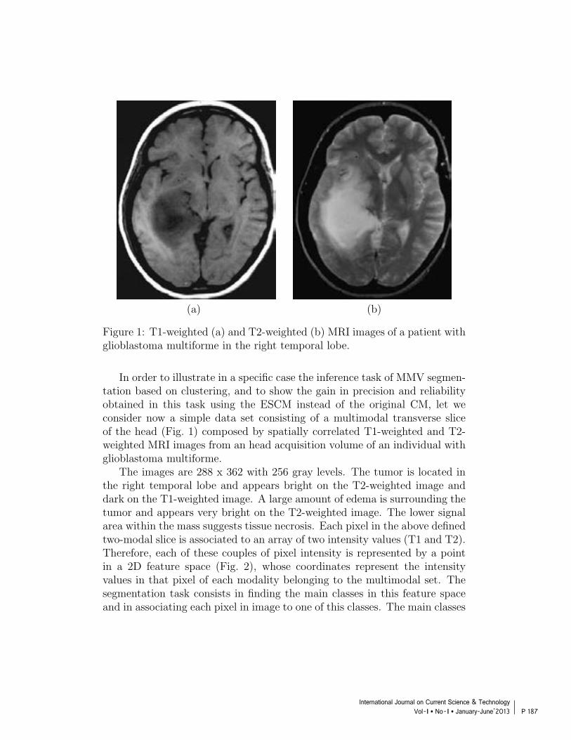
P 187International Journal on Current Science & Technology
Vol - I l No- I l January-June’2013
(a) (b)
Figure 1: T1-weighted (a) and T2-weighted (b) MRI images of a patient withglioblastoma multiforme in the right temporal lobe.
In order to illustrate in a specific case the inference task of MMV segmen-tation based on clustering, and to show the gain in precision and reliabilityobtained in this task using the ESCM instead of the original CM, let weconsider now a simple data set consisting of a multimodal transverse sliceof the head (Fig. 1) composed by spatially correlated T1-weighted and T2-weighted MRI images from an head acquisition volume of an individual withglioblastoma multiforme.
The images are 288 x 362 with 256 gray levels. The tumor is located inthe right temporal lobe and appears bright on the T2-weighted image anddark on the T1-weighted image. A large amount of edema is surrounding thetumor and appears very bright on the T2-weighted image. The lower signalarea within the mass suggests tissue necrosis. Each pixel in the above definedtwo-modal slice is associated to an array of two intensity values (T1 and T2).Therefore, each of these couples of pixel intensity is represented by a pointin a 2D feature space (Fig. 2), whose coordinates represent the intensityvalues in that pixel of each modality belonging to the multimodal set. Thesegmentation task consists in finding the main classes in this feature spaceand in associating each pixel in image to one of this classes. The main classes
17
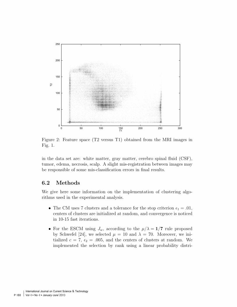
P 188International Journal on Current Science & Technology Vol - I l No- I l January-June’2013
0
50
100
150
200
250
0 50 100 150 200 250 300
T2
T1
Figure 2: Feature space (T2 versus T1) obtained from the MRI images inFig. 1.
in the data set are: white matter, gray matter, cerebro spinal fluid (CSF),tumor, edema, necrosis, scalp. A slight mis-registration between images maybe responsible of some mis-classification errors in final results.
6.2 Methods
We give here some information on the implementation of clustering algo-rithms used in the experimental analysis.
• The CM uses 7 clusters and a tolerance for the stop criterion ǫ1 = .01,centers of clusters are initialized at random, and convergence is noticedin 10-15 fast iterations.
• For the ESCM using Jw, according to the µ/λ = 1/7 rule proposedby Schwefel [24], we selected µ = 10 and λ = 70. Moreover, we ini-tialized c = 7, ǫ2 = .005, and the centers of clusters at random. Weimplemented the selection by rank using a linear probability distri-
18

P 189International Journal on Current Science & Technology
Vol - I l No- I l January-June’2013
4500
5000
5500
6000
6500
7000
0 5 10 15 20 25 30 35 40
best
indi
vidu
al c
ost f
unct
ion
iteration
Figure 3: Cost function of best individuals versus iteration of ESCM.
Figure 4: Segmentation obtained by the CM algorithm with 7 clusters.
19

P 190International Journal on Current Science & Technology Vol - I l No- I l January-June’2013
Figure 5: Segmentation obtained by the ESCM algorithm using Jw and with7 clusters.
bution with negative slope, while the intermediate recombination isimplemented as the average of components of parents.
• The implementation of ESCM using Js is identical to the previous one,with the obvious exception of the objective function. A typical plotof J best
s is presented in Fig. 3. Using ∆J bests /J best
s ≤ ǫ2 as the stopcondition, the ESCM ends in 15 iteration.
6.3 Results and Discussion
Let us compare the results produced by the ESCM clustering algorithm andby the standard C-Means (CM) algorithm.
In Fig. 4 the results of the unsupervised segmentation with the CM al-gorithm are shown. CM almost correctly defines scalp and white matter.Nevertheless it produces mistakes in classification of gray matter and edemain the left side of brain, and especially is not able to separate tumor, necrosisand CSF. Similar results are obtained by the basic ESCM with the standardcost function Jw (Fig. 5). Nevertheless, as an important difference, from
20

P 191International Journal on Current Science & Technology
Vol - I l No- I l January-June’2013
Figure 6: Segmentation obtained by the ESCM algorithm using Js and with7 clusters.
a large number of tests, ESCM results to be largely more stable than CMwith respect to the positions of centroids and to the extension of clustersin the feature space. Eventually, by using the newly defined scaled global
error function Js to take into account the cardinality of clusters, the resultsof ESCM (Fig. 6) dramatically improve. Actually, we may notice that, incomparison with CM, and with the basic version of ESCM, the final versionof ESCM correctly distinguishes between tumor and CSF, and within thetumor region is able to find the necrosis region. Correct definition of scalpand white matter and misclassification in the left side of the brain remainsas from CM.
7 Conclusions
The C-Means (CM) [6], while is an efficient approximation of the maximumlikelihood procedure for estimating the centers of clusters, shows some in-trinsic problems. In particular, it is subject to the problem of trapping inlocal minima of its objective function Jw (Eq. 16). This locality in search-
21
P 192International Journal on Current Science & Technology Vol - I l No- I l January-June’2013
ing for minima is a main limitation, in particular when we try to apply thisalgorithm as the basis for inference procedures.
In order to overcome the limits of C-Means, we have proposed in thispaper a novel clustering algorithm based on the application of an EvolutionStrategy (ES) [19, 25, 1] to the search for the global minimum (EvolutionStrategy based C-Means or ESCM algorithm).
The ESCM is based on a (µ, λ)-ES strategy where the object variablesof genotypes are the centers of clusters. The implementation of the (µ, λ)-ES strategy is quite standard, but before mixing object variables of parentsusing discrete recombination crossover, they are re-indexed, in such a waycenters with same index are likely to correspond to the same cluster.
It is worth noting that it is easy to make variants to the basic ESCM. Forinstance, with the straightforward change of Jw with the scaled global errorfunction Js (Eq. 23) it is possible to reduce the interference of big blobs tothe localization of the centers of small clusters.
In this paper we considered a complex inference processes based on clus-tering consisting in multimodal medical volumes (MMV) segmentation. Thisapproach has been shown to be very robust to noise and able to process com-plementary information carried by each image (e.g. functional or anatom-ical) [4]. In this inference task, devoted to aggregate voxels with similarproperties (corresponding to the different anatomical and/or pathologicaltissues) in the different diagnostic imaging volumes, clustering is performedin a multidimensional space where each independent dimension is a partic-ular volumetric image. Nevertheless, the used clustering method itself mustbe well founded in statistics and must be not limited by intrinsic problems,such as the problem of local optima in CM. Moreover, many bias effects (due,e.g., to heterogeneous clusters and to partial volume effect during acquisition)must be taken into account in considering clustering for the segmentation ofmedical images.
We have implemented the ESCM algorithm as a clustering module of thepreviously described graphical interactive system supporting the physicianfor the full sequence of analysis of multimodal medical volumes.
In the experimental results presented in the paper, we have comparedthe segmentation obtained by the application of CM, ESCM using Jw andESCM using Js to a simple data set consisting of a multimodal transverseslice of the head (Fig. 1) composed by spatially correlated T1-weighted andT2-weighted MRI images from an head acquisition volume of an individualwith glioblastoma multiforme.
22

P 193International Journal on Current Science & Technology
Vol - I l No- I l January-June’2013
The two implementations of ESCM give more stable solutions than CMwith respect to the positions of centroids and the extension of clusters inthe feature space. In particular, the ESCM using Js, as is able to takeinto account the cardinality of clusters, dramatically improves the quality ofsegmentation results.
Acknowledgments
The images are from the BrighamRAD Teaching Case Database of the De-partment of Radiology at Brigham and Women’s Hospital in Boston.
References
[1] T. Baeck. Evolutionary Algorithms in Theory and Practice: Evolution
Strategies, Evolutionary Programming, Genetic Algorithm. Oxford Uni-versity Press, 1996.
[2] A.M. Bensaid, L.O. Hall, L.P. Clarke, and R.P. Velthuizen. MRI seg-mentation using supervised and unsupervised methods. In Proc. 13th
IEEE Eng. Med. Biol. Conf., pages 483–489, Orlando, 1991. IEEE.
[3] J.C. Bezdek. Pattern Recognition with Fuzzy Objective Function Algo-
rithms. Plenum Press, New York, 1981.
[4] J.C. Bezdek, L.O. Hall, and L.P. Clarke. Review of MR image segmen-tation techniques using pattern recognition. Med. Phys., 20:1033–1048,1993.
[5] P. Bogus, A. Massone, and F. Masulli. A Simulated Annealing C-MeansClustering Algorithm. In F. Masulli and R. Parenti, editors, Proceedingof SOCO’99 ICSC Symposium on Soft Computing - Genova, pages 534–540, Millet, Canada, 1999. ICSC.
[6] R.O. Duda and P.E. Hart. Pattern Classification and Scene Analysis.Wiley, New York, 1973.
[7] F. Firenze and P. Morasso. The capture effect model: a new approach toself-organized clustering. In Sixth International Conference. Neural Net-
works and their Industrial and Cognitive Applications. NEURO-NIMES
23

P 194International Journal on Current Science & Technology Vol - I l No- I l January-June’2013
93 Conference Proceedings and Exhibition Catalog, pages 65–54, Nimes,France, 1993.
[8] G. Gerig, J. Martin, R. Kikinis, O. Kubler, M. Shenton, and F.A. Jolesz.Unsupervised tissue type segmentation of 3D dual-echo MR head data.Im. Vis. Comput., 10:349–360, 1992.
[9] E. T. Jaynes. Information theory and statistical mechanics. Physical
Review, 106:620–630, 1957.
[10] Z-X Ji, Q-S Sun, D-S Xia. A modied possibilistic fuzzy c-means clus-tering algorithm for bias field estimation and segmentation of brain MRimage. Computerized Medical Imaging and Graphics 35 38–397, 2011.
[11] S. Kirkpatrick, C.D. Gelatt, and M.P. Vecchi. Optimization by simulatedannealing. Science, 220:661–680, 1983.
[12] R. Krishnapuram and J.M. Keller. A possibilistic approach to clustering.IEEE Transactions on Fuzzy Systems, 1:98–110, 1993.
[13] R. Krishnapuram and J.M. Keller. The Possibilistic C-Means algorithm:Insights and recommendations. IEEE Transactions on Fuzzy Systems,4:385–393, 1996.
[14] H. Mahmoud, F. Masulli, S. Rovetta. A Fuzzy Clustering Segmenta-tion Approach for Feature-Based Medical Image Registration. In Proc.
CIBB 2012, 9-th International Meeting on Computational Intelligence
Methods for Bioinformatics and Biostatistics, Houston, Tx, USA, CIBBProceedings Series, ISBN 978-88-906437-1-2, 2012.
[15] M.N. Maisey and et al. Synergistic imaging. Eur. J. Nucl. Med.,19:1002–1005, 1992.
[16] F. Masulli, P. Bogus, A. Schenone, and M. Artuso. Fuzzy clusteringmethods for the segmentation of multivariate images. In M. Mares,R. Mesia, V. Novak, J. Ramik, and A. Stupnanova, editors, Proceed-ings of the 7th International Fuzzy Systems Association Word Congress
IFSA’97, volume III, pages 123–128, Prague, 1997. Academia.
[17] F. Masulli and A. Schenone. A fuzzy clustering based segmetation sys-tem as support to diagnosis in medical imaging. Artificial Intelligence
in Medicine 16, 129–147, 1999.
24
P 195International Journal on Current Science & Technology
Vol - I l No- I l January-June’2013
[18] S. Miyamoto and M. Mukaidono. Fuzzy C-Means as a regularizationand maximum entropy approach. In M. Mares, R. Mesia, V. Novak,J. Ramik, and A. Stupnanova, editors, Proceedings of the 7th Interna-
tional Fuzzy Systems Association Word Congress IFSA’97, volume III,pages 86–91, Prague, 1997. Academia.
[19] I. Rechenberg. Evolutionsstrategie: Optimierung technischer Systeme
nach Prinzipien der biologischen Evolution. Frommann-Holzboog Ver-lag, Stuttgart, 1973.
[20] K. Rose, E. Gurewitz, and G. Fox. A deterministic annealing approachto clustering. Pattern Recognition Letters, 11:589–594, 1990.
[21] K. Rose, E. Gurewitz, and G. Fox. Constrained clustering as an opti-mization method. IEEE Transaction on Pattern Analysis and Machine
Intelligence, 15:785–794, 1993.
[22] A. Schenone, F. Firenze, F. Acquarone, M. Gambaro, F. Masulli, andL. Andreucci. Segmentation of multivariate medical images via unsuper-vised clustering with adaptive resolution. Computerized Medical Imaging
and Graphics, 20:119–129, 1996.
[23] K. E. Parsopoulos, M. N. Vrahatis. Recent approaches to global opti-mization problems through Particle Swarm Optimization. Natural Com-
puting 1(2-3):235-306, 2002.
[24] H.P. Schwefel. Collective phenomena in evolutionary systems. InPreprints of the 31-th annual meeting of the International Society for
General Systems Research, volume 2, pages 1025–1033, Budapest, 1988.
[25] H.P. Schwefel. Evolution and Optimum Seeking. Wiley, 1995.
[26] A. Tikhonov and V. Arsenin. Solutions of ill-posed problems. Winstonand Sons, New York, 1997.
[27] E.C.K. Tsao, J.C. Bezdek, and N.R. Pal. Fuzzy Kohonen clusteringnetworks. Pattern Recognition, 27(5):757–764, 1994.
25

P 196International Journal on Current Science & Technology Vol - I l No- I l January-June’2013
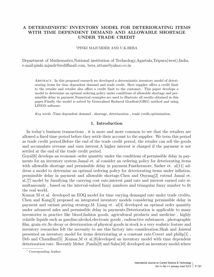
P 197International Journal on Current Science & Technology
Vol - I l No- I l January-June’2013
A DETERMINISTIC INVENTORY MODEL FOR DETERIORATING ITEMSWITH TIME DEPENDENT DEMAND AND ALLOWABLE SHORTAGE
UNDER TRADE CREDIT
†PINKI MAJUMDER AND U.K.BERA
Department of Mathematics,National institution of Technology,Agartala,Tripura(west),India,e-mail:[email protected], bera [email protected]
Abstract. In this proposed research we developed a deterministic inventory model of deteri-orating items for time dependent demand and trade credit. Here supplier offers a credit limitto the retailer and retailer also offers a credit limit to the customer. This paper develops amodel to determine an optimal ordering policy under conditions of allowable shortage and per-missible delay in payment.Numerical examples are used to illustrate all results obtained in thispaper.Finally the model is solved by Generalised Reduced Gradient(GRG) method and usingLINGO software.
Key words :Time dependent demand , shortage, deterioration , trade credit,optimization.
1. Introduction
In today’s business transactions , it is more and more common to see that the retailers areallowed a fixed time period before they settle their account to the supplier. We term this periodas trade credit period.Before the end of the trade credit period, the retailer can sell the goodsand accumulate revenue and earn interest.A higher interest is charged if the payment is notsettled at the end of the trade credit period.Goyal[6] develops an economic order quantity under the conditions of permissible delay in pay-ments for an inventory system.Jamal et. al consider an ordering policy for deteriorating itemswith allowable shortage and permissible delay in payment.Funthermore, Sarker et. al[11] ad-dress a model to determine an optimal ordering policy for deteriorating items under inflation,permissible delay in payment and allowable shortage.Chen and Ouyang[2] extend Jamal et.al.[7] model by fuzzifying the carrying cost rate,interest paid rate and interest earned rate si-multaneously , based on the interval-valued fuzzy numbers and triangular fuzzy number to fitthe real world.Kumar M et al. developed an EOQ model for time varying demaqnd rate under trade credits.Chen and Kang[3] proposed an integrated inventory models considering permissible delay inpayment and variant pricing strategy,M. Liang et. al[4] developed an optimal order quantityunder advanced sales and permissible delay in payments.Deterioration is applicable to manyinventories in practice like blood,fashion goods, agricultural products and medicine , highlyvolatile liquids such as gasoline;alcohol,electronic goods , radioactive substances , photographicfilm, grain etc.So decay or deterioration of physical goods in stock is a very realistic feature andinventory researches felt the necessity to use this factory into consideration.Shah and Jaiswalpresented an inventory model for items deteriorating at a constant rate.Covert and philip[1] ,Deb and Chaudhuri[5] ,Kumar,M et al.[8]developed an inventory model with time dependentdeterioration rate. Recently Meher ,Panda[9] and Sahu[10] developed an inventory model where
† Corresponding Author.1

P 198International Journal on Current Science & Technology Vol - I l No- I l January-June’2013
2 Pinki Majumder and U.K.Bera
demand is a weibull function of time.In the classical inventory models the demand rate is assumed to be a constant . In reality ,demand for physical goals may be time dependent and price dependent. Meher , Panda andSahu[10] develops inventory model where demand is a function of time.In this paper we establish an deterministic inventory model with allowable shortage , timedependent demand , weibull deterioration and two trade credit period. Here we derive theoptimal value of cycle time which minimize the total average cost. Lastly numerical examplesare set to illustrate all results obtained in this paper.
2. Assumptions and notationThe following notations and assumptions are used for the development of proposed model.2a. Notation
(i) D(t)=a(1-bt); the annual demand as a decreasing function of time where a > 0 is fixeddemand and b(0 < b < 1) denotes the rate of demand.
(ii) C = The unit purchase cost.(iii) S = The unit selling cost with (S > C).(iv) h= The inventory holding cost per year excluding interest charges.(v) A = The ordering cost per order.(vi) P = The unit shortage cost.(vii) Q(t) = The order quantity at time t = 0.(viii) θ(t) = The deteriorating rate which is a weibull function of time as θ(t) =αβtβ−1 where
0 < α << 1, β > 0 and t > 0(ix) M= Retailer’s trade credit period offered by the supplier in years.(x) N = Customer’s trade period offered by the retailer in years.(xi) Ic = Interest charges payable per $ per year to the supplier.(xii) Ie = Interest earned per $ per year.(xiii) I(t) = Inventory level at time t.(xiv) T1 = Length of the period with positive stock of the item.(xv) T2 = Length of the period with negative stock of the item.(xvi) T = Length of the replenishment cycle . T = T1 + T2
(xvii) Z(T1, T2) : Total Inventory cost when the length of period with positive stock of theitem is T1 and the length of the period with negative stock of the item is T2.
(xviii) Z1(T1, T2) : Total relevant cost per unit time when N ≤ M ≤ T1 < T .(xix) Z2(T1, T2) : Total relevant cost per unit time when N ≤ T1 ≤ M < T .(xx) Z3(T1, T2) : Total relevant cost per unit time when 0 ≤ T1 ≤ N ≤ M < T .(xxi) T ∗
1= Optimal value of T1.
(xxii) T ∗2= Optimal value of T2.
2b. Assumption
(i) The inventory system under consideration deals with the single item.(ii) The planning horizon is infinite.(iii) The demand of the product is declining function of time.(iv) Shortages are allowed.(v) Ic ≥ Ie , S ≥ C, M ≥ N .(vi) The supplier offers the full trade credit to the retailer.When T1 ≥ M ,the account is
settled at T1 = M ,the retailer pays off all units sold and keeps his/her profits, and startspaying for the interest charges on the items in stock with rate Ic .When T1 ≤ M ,theaccount is settled at T1 = M and the retailer no need to pay any interest on the stock.

P 199International Journal on Current Science & Technology
Vol - I l No- I l January-June’2013
A deterministic inventory model.......... allowable shortage under trade credit 3
(vii) The retailer can accumulate revenue and earn interest after his/her customer pays forthe amount of purchasing cost to the retailer until the end of the trade credit periodoffered by the supplier . That is , the retailer can accumulate revenue and earn interestduring the period N to M with rate Ie under the condition of trade credit.
(viii) The deteriorated units can neither be repaired nor replaced during the cycle time.
3. Mathematical Formulation
The inventory level I(t) depletes to meet the demand and deterioration. The rate of change ofinventory level is governed by the following differential equationdI(t)dt
+ θI(t) = −D(t) ,0 ≤ t ≤ T (1)
which is equivalent to dI(t)dt
+ αβtβ−1I(t) = −a(1− bt) ,0 ≤ t ≤ T (2)with the initial condition I(0) = Q and the boundary condition I(T1) = 0Consequently, the solution of (2) is given by
I(t) = ae−αtβ [ αβ+1
(T β+1
1−tβ+1)− bα
β+2(T β+2
1−tβ+2)− b
2(T 2
1−t2)+(T1−t)] , 0 ≤ t ≤ T (3)
The order quantity is Q = I(0) = a[ αβ+1
T β+1
1− bα
β+2T β+2
1− bT 2
1
2+ T1 ] (4)
the total cost of inventory system per time unit include the following :(a) Ordering cost : A
(T1+T2)
(b) Deterioration cost per unit time : Caα(T1+T2)
[Tβ+11
β+1− bTβ+2
1
β+2]
(c)Inventory holding cost per unit time:ah
(T1+T2)[ α2b(β+1)(2β+3)
T(2β+3)
1− α2
2(β+1)2T
(2β+2)
1− bαβ
(β+1)(β+3)T
(β+3)
1+ αβ
(β+1)(β+2)T
(β+2)
1− bT 3
1
3+
T 21
2]
(d)Shortage cost = − P(T1+T2)
T∫
T1
I(t)dt
= − P(T1+T2)
T∫
T1
(1− αtβ)[ αβ+1
(T β+1
1− tβ+1)− bα
β+2(T β+2
1− tβ+2)− b
2(T 2
1− t2) + (T1 − t)]dt
= P(T1+T2)
[ αβ(β+1)(β+2)
T(β+2)
1− bαβ
(β+1)(β+3)T
(β+3)
1+ α2b
(β+1)(2β+3)T
(2β+3)
1− α2
2(β+1)2T 2β+2
1− bT 3
1
3+
T 21
2]+
P(T1+T2)
[ α2
β+1(T β+1
1
(T1+T2)β+1
β+1− (T1+T2)
2β+2
2β+2)− α2b
β+2(T β+2
1
(T1+T2)β+1
β+1− (T1+T2)
2β+3
2β+3)− αb
2(T 2
1
(T1+T2)β+1
β+1−
(T1+T2)β+3
β+3)+α(T1
(T1+T2)β+1
β+1− (T1+T2)
β+2
β+2)− α
β+1(T β+1
1(T1+T2)− (T1+T2)
β+2
β+2)+ bα
β+2(T β+2
1(T1+T2)−
(T1+T2)β+3
β+3) + b
2(T 2
1(T1 + T2)− (T1+T3)
3
3)− (T1(T1 + T2)− (T1+T2)
2
2)]
Regarding interest charges and earned three cases may arise based on the length of M,N, T1.The three cases are as followsCase1 : N ≤ M ≤ T1 < TCase2 : N ≤ T1 ≤ M < TCase3 : T1 ≤ N ≤ M < T
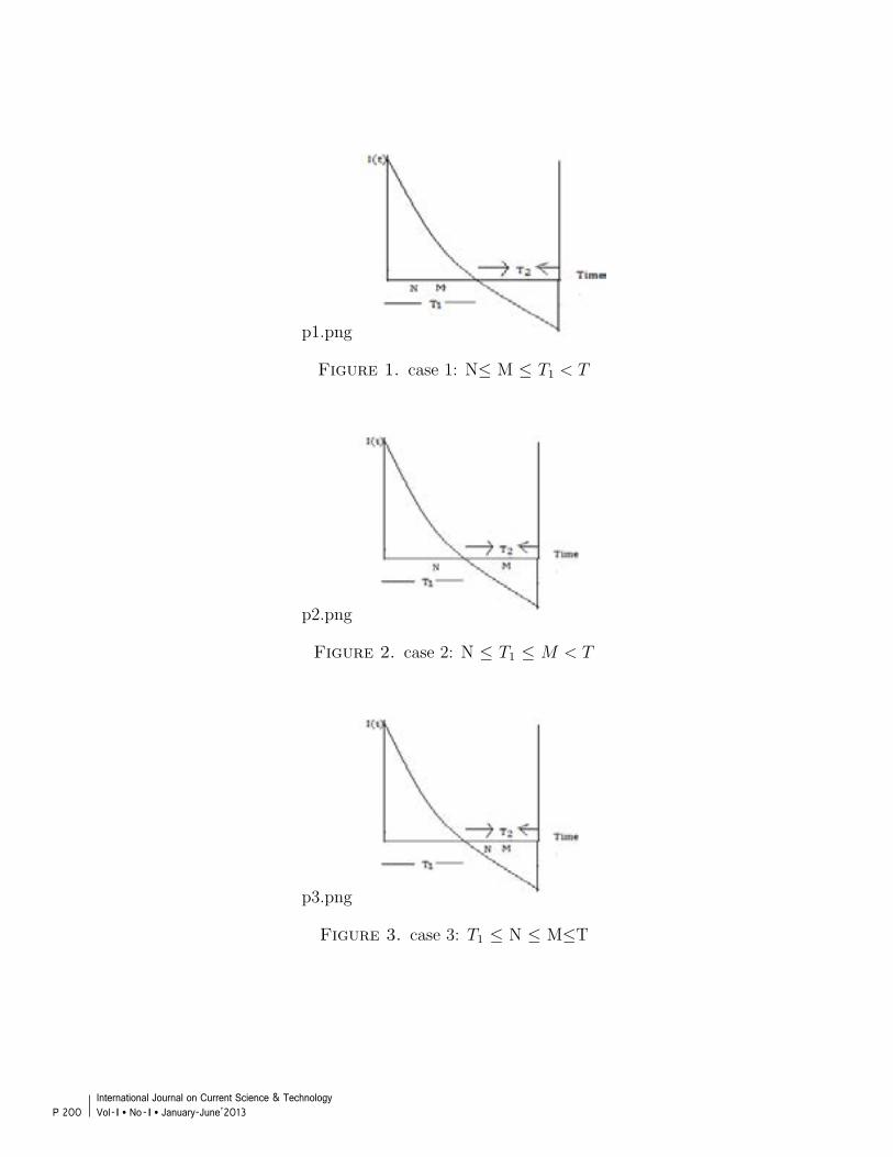
P 200International Journal on Current Science & Technology Vol - I l No- I l January-June’2013
4 Pinki Majumder and U.K.Bera
p1.png
Figure 1. case 1: N≤ M ≤ T1 < T
p2.png
Figure 2. case 2: N ≤ T1 ≤ M < T
p3.png
Figure 3. case 3: T1 ≤ N ≤ M≤T

P 201International Journal on Current Science & Technology
Vol - I l No- I l January-June’2013
A deterministic inventory model.......... allowable shortage under trade credit 5
4. According to given assumption,there are three cases to occur in interest charged for theitems kept in stock per year.
Case 1. N ≤ M ≤ T1 < T
Annual interest payable= CIc(T1+T2)
T1∫
M
I(t)dt
= CIca(T1+T2)
T1∫
M
(1− αtβ)[ αβ+1
(T β+1
1− tβ+1)− bα
β+2(T β+2
1− tβ+2)− b
2(T 2
1− t2) + (T1 − t)]dt
= CIca(T1+T2)
[ α2b(β+1)(2β+3)
T(2β+3)
1− α2
2(β+1)2T
(2β+2)
1− bαβ
(β+1)(β+3)T
(β+3)
1+ αβ
(β+1)(β+2)T
(β+2)
1− bT 3
1
3+
T 21
2−
(αT
(β+1)1
(β+1)−αβT
(β+2)1
(β+2)− bT 2
1
2+T1)(M−αM(β+1)
(β+1))− αβ
(β+1)(β+2)Mβ+2+ αβb
2(β+2)(β+3)Mβ+3− α2
(β+1)(2β+2)M2β+2+
α2b(β+2)(2β+3)
M2β+3 − bM3
6+ M2
2]
Case2. N ≤ T1 ≤ M < TIn this case annual interest payable = 0Case 3. T1 ≤ N ≤ M < TIn this case annual interest payable = 0
5. According to given assumption,three cases will occur in interest earned per year.case 1. N ≤ M ≤ T1 < T
The annual interest earned = SIe(T1+T2)
[a(1− bT2)T2(M −N) +M∫
N
a(1− bt)tdt]
= SIe(T1+T2)
[a(1− bT2)T2(M −N) + a(M2
2− bM3
3− N2
2+ bN3
3)]
case 2. N ≤ T1 ≤ M < T
The annual interest earned = SIe(T1+T2)
[a(1−bT2)T2(M−N)+a(1−bT1)T1(M−T1)+T1∫
N
a(1− bt)tdt]
= SIe(T1+T2)
[a(1− bT2)T2(M −N) + a(T 21
2− bT 3
1
3− N2
2+ bN3
3) + a(1− bT1)T1(M − T1)]
case 3. T1 ≤ N ≤ M < TThe annual interest earned = SIe
(T1+T2)[a(1− bT2)T2(M −N) + a(1− bT1)T1(M −N)]
The annual total cost incurred by the retailerZ(T1, T2) = Setup cost + Holding cost + Purchasing cost + Shortage cost +Interest payable -Interest earned
where Z1(T1, T2) =A
(T1+T2)+ Caα
(T1+T2)[Tβ+11
β+1− bTβ+2
1
β+2] + ah
(T1+T2)[ α2b(β+1)(2β+3)
T(2β+3)
1− α2
2(β+1)2T
(2β+2)
1−
bαβ(β+1)(β+3)
T(β+3)
1+ αβ
(β+1)(β+2)T
(β+2)
1− bT 3
1
3+
T 21
2]+
+ CIca(T1+T2)
[ α2b(β+1)(2β+3)
T(2β+3)
1− α2
2(β+1)2T
(2β+2)
1− bαβ
(β+1)(β+3)T
(β+3)
1+ αβ
(β+1)(β+2)T
(β+2)
1− bT 3
1
3+
T 21
2−
(αT
(β+1)1
(β+1)−αβT
(β+2)1
(β+2)− bT 2
1
2+T1)(M−αM(β+1)
(β+1))− αβ
(β+1)(β+2)Mβ+2+ αβb
2(β+2)(β+3)Mβ+3− α2
(β+1)(2β+2)M2β+2+
α2b(β+2)(2β+3)
M2β+3 − bM3
6+ M2
2]
+ P(T1+T2)
[ αβ(β+1)(β+2)
T(β+2)
1− bαβ
(β+1)(β+3)T
(β+3)
1+ α2b
(β+1)(2β+3)T
(2β+3)
1− α2
2(β+1)2T 2β+2
1− bT 3
1
3+
T 21
2] +
P(T1+T2)
[ α2
β+1(T β+1
1
(T1+T2)β+1
β+1− (T1+T2)
2β+2
2β+2)− α2b
β+2(T β+2
1
(T1+T2)β+1
β+1− (T1+T2)
2β+3
2β+3)− αb
2(T 2
1
(T1+T2)β+1
β+1−

P 202International Journal on Current Science & Technology Vol - I l No- I l January-June’2013
6 Pinki Majumder and U.K.Bera
(T1+T2)β+3
β+3)+α(T1
(T1+T2)β+1
β+1− (T1+T2)
β+2
β+2)− α
β+1(T β+1
1(T1+T2)− (T1+T2)
β+2
β+2)+ bα
β+2(T β+2
1(T1+T2)−
(T1+T2)β+3
β+3) + b
2(T 2
1(T1 + T2)− (T1+T3)
3
3)− (T1(T1 + T2)− (T1+T2)
2
2)]
− SIe(T1+T2)
[a(1− bT2)T2(M −N) + a(M2
2− bM3
3− N2
2+ bN3
3)]
where Z2(T1, T2) =A
(T1+T2)+ Caα
(T1+T2)[Tβ+11
β+1− bTβ+2
1
β+2]+ ah
(T1+T2)[ α2b(β+1)(2β+3)
T(2β+3)
1− α2
2(β+1)2T
(2β+2)
1−
bαβ(β+1)(β+3)
T(β+3)
1+ αβ
(β+1)(β+2)T
(β+2)
1− bT 3
1
3+
T 21
2]+
P(T1+T2)
[ αβ(β+1)(β+2)
T(β+2)
1− bαβ
(β+1)(β+3)T
(β+3)
1+ α2b
(β+1)(2β+3)T
(2β+3)
1− α2
2(β+1)2T 2β+2
1− bT 3
1
3+
T 21
2] +
P(T1+T2)
[ α2
β+1(T β+1
1
(T1+T2)β+1
β+1− (T1+T2)
2β+2
2β+2)− α2b
β+2(T β+2
1
(T1+T2)β+1
β+1− (T1+T2)
2β+3
2β+3)− αb
2(T 2
1
(T1+T2)β+1
β+1−
(T1+T2)β+3
β+3)+α(T1
(T1+T2)β+1
β+1− (T1+T2)
β+2
β+2)− α
β+1(T β+1
1(T1+T2)− (T1+T2)
β+2
β+2)+ bα
β+2(T β+2
1(T1+T2)−
(T1+T2)β+3
β+3) + b
2(T 2
1(T1 + T2)− (T1+T3)
3
3)− (T1(T1 + T2)− (T1+T2)
2
2)]
− SIe(T1+T2)
[a(1− bT2)T2(M −N) + a(T 21
2− bT 3
1
3− N2
2+ bN3
3) + a(1− bT1)T1(M − T1)]
Z3(T1, T2) = A(T1+T2)
+ Caα(T1+T2)
[Tβ+11
β+1− bTβ+2
1
β+2] + ah
(T1+T2)[ α2b(β+1)(2β+3)
T(2β+3)
1− α2
2(β+1)2T
(2β+2)
1−
bαβ(β+1)(β+3)
T(β+3)
1+ αβ
(β+1)(β+2)T
(β+2)
1− bT 3
1
3+
T 21
2]+
P(T1+T2)
[ αβ(β+1)(β+2)
T(β+2)
1− bαβ
(β+1)(β+3)T
(β+3)
1+ α2b
(β+1)(2β+3)T
(2β+3)
1− α2
2(β+1)2T 2β+2
1− bT 3
1
3+
T 21
2] +
P(T1+T2)
[ α2
β+1(T β+1
1
(T1+T2)β+1
β+1− (T1+T2)
2β+2
2β+2)− α2b
β+2(T β+2
1
(T1+T2)β+1
β+1− (T1+T2)
2β+3
2β+3)− αb
2(T 2
1
(T1+T2)β+1
β+1−
(T1+T2)β+3
β+3)+α(T1
(T1+T2)β+1
β+1− (T1+T2)
β+2
β+2)− α
β+1(T β+1
1(T1+T2)− (T1+T2)
β+2
β+2)+ bα
β+2(T β+2
1(T1+T2)−
(T1+T2)β+3
β+3) + b
2(T 2
1(T1 + T2)− (T1+T3)
3
3)− (T1(T1 + T2)− (T1+T2)
2
2)]
− SIe(T1+T2)
[a(1− bT2)T2(M −N) + a(1− bT1)T1(M −N)]
Since Z1(M,T2) = Z2(M,T2)Z2(N, T2) = Z3(N, T2)Therefore Z(T1, T2) is continuous and well defindedAll Z1(T1, T2), Z2(T1, T2), Z3(T1, T2) are defined on T1 > 0, T2 > 0.6. The determinations of the optimal solution of Z(T1, T2)The optimal solutions (T1, T2) of Z1(T1, T2)can be determined by equations
∂Z1(T1,T2)
∂T1= 0 (1)
∂Z1(T1,T2)
∂T2= 0 (2)
(1) implies
− A(T1+T2)
2− Caα(T1+T2)
2 [Tβ+11
β+1− bTβ+2
1
β+2]− ah
(T1+T2)2 [
α2b(β+1)(2β+3)
T(2β+3)
1− α2
2(β+1)2T
(2β+2)
1− bαβ
(β+1)(β+3)T
(β+3)
1+
αβ(β+1)(β+2)
T(β+2)
1− bT 3
1
3+
T 21
2]
− CIca(T1+T2)
2 [α2b
(β+1)(2β+3)T
(2β+3)
1− α2
2(β+1)2T
(2β+2)
1− bαβ
(β+1)(β+3)T
(β+3)
1+ αβ
(β+1)(β+2)T
(β+2)
1− bT 3
1
3+
T 21
2−
(αT
(β+1)1
(β+1)−αbT
(β+2)1
(β+2)− bT 2
1
2+T1)(M−αM(β+1)
(β+1))− αβ
(β+1)(β+2)Mβ+2+ αβb
2(β+2)(β+3)Mβ+3− α2
(β+1)(2β+2)M2β+2+
α2b(β+2)(2β+3)
M2β+3 − bM3
6+ M2
2]
+ SIe(T1+T2)
2 [a(1− bT2)T2(M −N) + a(M2
2− bM3
3− N2
2+ bN3
3)]
− P(T1+T2)
2 [αβ
(β+1)(β+2)T
(β+2)
1− bαβ
(β+1)(β+3)T
(β+3)
1+ α2b
(β+1)(2β+3)T
(2β+3)
1− α2
2(β+1)2T 2β+2
1− bT 3
1
3+
T 21
2]−
P(T1+T2)
2 [α2
β+1(T β+1
1
(T1+T2)β+1
β+1− (T1+T2)
2β+2
2β+2)− α2b
β+2(T β+2
1
(T1+T2)β+1
β+1− (T1+T2)
2β+3
2β+3)− αb
2(T 2
1
(T1+T2)β+1
β+1−

P 203International Journal on Current Science & Technology
Vol - I l No- I l January-June’2013
A deterministic inventory model.......... allowable shortage under trade credit 7
(T1+T2)β+3
β+3)+α(T1
(T1+T2)β+1
β+1− (T1+T2)
β+2
β+2)− α
β+1(T β+1
1(T1+T2)− (T1+T2)
β+2
β+2)+ bα
β+2(T β+2
1(T1+T2)−
(T1+T2)β+3
β+3) + b
2(T 2
1(T1 + T2)− (T1+T3)
3
3)− (T1(T1 + T2)− (T1+T2)
2
2)]+
P(T1+T2)
[ αβ(β+1)
T β+1
1− bαβ
(β+1)T β+2
1+ α2b
(β+1)T 2β+2
1− α2
(β+1)T 2β+1
1− bT 2
1+T1]+
P(T1+T2)
[ α2
(β+1)(T β+1
1(T1+
T2)β + (T1 + T2)
β+1T β1− (T1 + T2)
2β+1)− α2b(β+2)
(T β+2
1(T1 + T2)
β + (T1+T2)β+1
β+1(β + 2)T β+1
1− (T1 +
T2)2β+2)− αb
2( (T1+T2)
β+1
β+12T1+(T1+T2)
βT 2
1− (T1+T2)
β+2)+α((T1+T2)βT1+
(T1+T2)β+1
(β+1)− (T1+
T2)β+1)− α
(β+1)((β+1)T β
1(T1+T2)+T β+1
1− (T1+T2)
β+1)+ bαβ+2
((β+2)T β+1
1(T1+T2)+T β+2
1−
(T1 + T2)β+2) + b
2(T 2
1+ (T1 + T2)2T1 − (T1 + T2)
2)− (T1 + (T1 + T2)− (T1 + T2))]
+ Caα(T1+T2)
(T β1−bT β+1
1)+ ah
(T1+T2)[ αβ(β+1)
T β+1
1− bαβ
(β+1)T β+2
1+ α2b
(β+1)T 2β+2
1− α2
(β+1)T 2β+1
1−bT 2
1+T1]+
aCIc(T1+T2)
[ α2b(β+1)
T 2β+2
1− α2
(β+1)T 2β+1
1− αβb
(β+1)T β+2
1+ αβ
(β+1)T β+1
1− bT 2
1+ T1 − (αT β
1− αbT β+1
1− bT1 +
1)(M − αMβ+1
(β+1))] = 0 (3)
Now (2) implies
− A(T1+T2)
2 − Caα(T1+T2)
2 [Tβ+11
β+1− bTβ+2
1
β+2]− ah
(T1+T2)2 [
α2b(β+1)(2β+3)
T(2β+3)
1− α2
2(β+1)2T
(2β+2)
1− bαβ
(β+1)(β+3)T
(β+3)
1+
αβ(β+1)(β+2)
T(β+2)
1− bT 3
1
3+
T 21
2]
− CIca(T1+T2)
2 [α2b
(β+1)(2β+3)T
(2β+3)
1− α2
2(β+1)2T
(2β+2)
1− bαβ
(β+1)(β+3)T
(β+3)
1+ αβ
(β+1)(β+2)T
(β+2)
1− bT 3
1
3+
T 21
2−
(αT
(β+1)1
(β+1)−αbT
(β+2)1
(β+2)− bT 2
1
2+T1)(M−αM(β+1)
(β+1))− αβ
(β+1)(β+2)Mβ+2+ αβb
2(β+2)(β+3)Mβ+3− α2
(β+1)(2β+2)M2β+2+
α2b(β+2)(2β+3)
M2β+3 − bM3
6+ M2
2]
+ SIe(T1+T2)
2 [a(1− bT2)T2(M −N) + a(M2
2− bM3
3− N2
2+ bN3
3)]− sIe
(T1+T2)[a(1− 2bT2)(M −N)]
− P(T1+T2)
2 [αβ
(β+1)(β+2)T
(β+2)
1− bαβ
(β+1)(β+3)T
(β+3)
1+ α2b
(β+1)(2β+3)T
(2β+3)
1− α2
2(β+1)2T 2β+2
1− bT 3
1
3+
T 21
2]−
P(T1+T2)
2 [α2
β+1(T β+1
1
(T1+T2)β+1
β+1− (T1+T2)
2β+2
2β+2)− α2b
β+2(T β+2
1
(T1+T2)β+1
β+1− (T1+T2)
2β+3
2β+3)− αb
2(T 2
1
(T1+T2)β+1
β+1−
(T1+T2)β+3
β+3) + α(T1
(T1+T2)β+1
β+1− (T1+T2)
β+2
β+2) − α
β+1(T β+1
1(T1 + T2) − (T1+T2)
β+2
β+2) + bα
β+2(T β+2
1(T1 +
T2)− (T1+T2)β+3
β+3)+ b
2(T 2
1(T1+T2)− (T1+T3)
3
3)− (T1(T1+T2)− (T1+T2)
2
2)]+ P
(T1+T2)[ α2
(β+1)(T β+1
1(T1+
T2)β− (T1+T2)
2β+1)− α2b(β+2)
(T β+2
1(T1+T2)
β− (T1+T2)2β+2)− αb
2((T1+T2)
βT 2
1− (T1+T2)
β+2)+
α((T1 + T2)βT1 − (T1 + T2)
β+1) − α(β+1)
(T β+1
1− (T1 + T2)
β+1) + bα(β+2)
(T β+2
1− (T1 + T2)
β+2) +b2(T 2
1− (T1 + T2)
2)− (T1 − (T1 + T2))] =0 (4)
The equation (3) and (4) gives the optimal value T ∗1and T ∗
2.
The optimal solutions (T1, T2) of Z2(T1, T2) can be determined by equations∂Z2(T1,T2)
∂T1= 0 (5)
∂Z2(T1,T2)
∂T2= 0 (6)
(5) implies
− A(T1+T2)
2 − Caα(T1+T2)
2 [Tβ+11
β+1− bTβ+2
1
β+2]− ah
(T1+T2)2 [
α2b(β+1)(2β+3)
T(2β+3)
1− α2
2(β+1)2T
(2β+2)
1− bαβ
(β+1)(β+3)T
(β+3)
1+
αβ(β+1)(β+2)
T(β+2)
1− bT 3
1
3+
T 21
2]
− P(T1+T2)
2 [αβ
(β+1)(β+2)T
(β+2)
1− bαβ
(β+1)(β+3)T
(β+3)
1+ α2b
(β+1)(2β+3)T
(2β+3)
1− α2
2(β+1)2T 2β+2
1− bT 3
1
3+
T 21
2]−
P(T1+T2)
2 [α2
β+1(T β+1
1
(T1+T2)β+1
β+1− (T1+T2)
2β+2
2β+2)− α2b
β+2(T β+2
1
(T1+T2)β+1
β+1− (T1+T2)
2β+3
2β+3)− αb
2(T 2
1
(T1+T2)β+1
β+1−

P 204International Journal on Current Science & Technology Vol - I l No- I l January-June’2013
8 Pinki Majumder and U.K.Bera
(T1+T2)β+3
β+3)+α(T1
(T1+T2)β+1
β+1− (T1+T2)
β+2
β+2)− α
β+1(T β+1
1(T1+T2)− (T1+T2)
β+2
β+2)+ bα
β+2(T β+2
1(T1+T2)−
(T1+T2)β+3
β+3) + b
2(T 2
1(T1 + T2)− (T1+T3)
3
3)− (T1(T1 + T2)− (T1+T2)
2
2)]+
P(T1+T2)
[ αβ(β+1)
T β+1
1− bαβ
(β+1)T β+2
1+ α2b
(β+1)T 2β+2
1− α2
(β+1)T 2β+1
1− bT 2
1+T1]+
P(T1+T2)
[ α2
(β+1)(T β+1
1(T1+
T2)β + (T1 + T2)
β+1T β1− (T1 + T2)
2β+1)− α2b(β+2)
(T β+2
1(T1 + T2)
β + (T1+T2)β+1
β+1(β + 2)T β+1
1− (T1 +
T2)2β+2)− αb
2( (T1+T2)
β+1
β+12T1+(T1+T2)
βT 2
1− (T1+T2)
β+2)+α((T1+T2)βT1+
(T1+T2)β+1
(β+1)− (T1+
T2)β+1)− α
(β+1)((β+1)T β
1(T1+T2)+T β+1
1− (T1+T2)
β+1)+ bαβ+2
((β+2)T β+1
1(T1+T2)+T β+2
1−
(T1 + T2)β+2) + b
2(T 2
1+ (T1 + T2)2T1 − (T1 + T2)
2)− (T1 + (T1 + T2)− (T1 + T2))]
+ Caα(T1+T2)
(T β1− bT β+1
1) + ah
(T1+T2)[ αβ(β+1)
T β+1
1− bαβ
(β+1)T β+2
1+ α2b
(β+1)T 2β+2
1− α2
(β+1)T 2β+1
1− bT 2
1+ T1]
+ SIe(T1+T2)
2 [a(1−bT2)T2(M−N)+a(T 21
2− bT 3
1
3−N2
2+ bN3
3)+a(1−bT1)T1(M−T1)]− SIe
(T1+T2)[a(T1−
bT 2
1) + a(1− bT1)(M − 2T1) + T1(M − T1)(−b)]=0 (7)
(6) implies
− A(T1+T2)
2 − Caα(T1+T2)
2 [Tβ+11
β+1− bTβ+2
1
β+2]− ah
(T1+T2)2 [
α2b(β+1)(2β+3)
T(2β+3)
1− α2
2(β+1)2T
(2β+2)
1− bαβ
(β+1)(β+3)T
(β+3)
1+
αβ(β+1)(β+2)
T(β+2)
1− bT 3
1
3+
T 21
2]
− P(T1+T2)
2 [αβ
(β+1)(β+2)T
(β+2)
1− bαβ
(β+1)(β+3)T
(β+3)
1+ α2b
(β+1)(2β+3)T
(2β+3)
1− α2
2(β+1)2T 2β+2
1− bT 3
1
3+
T 21
2]−
P(T1+T2)
2 [α2
β+1(T β+1
1
(T1+T2)β+1
β+1− (T1+T2)
2β+2
2β+2)− α2b
β+2(T β+2
1
(T1+T2)β+1
β+1− (T1+T2)
2β+3
2β+3)− αb
2(T 2
1
(T1+T2)β+1
β+1−
(T1+T2)β+3
β+3) + α(T1
(T1+T2)β+1
β+1− (T1+T2)
β+2
β+2) − α
β+1(T β+1
1(T1 + T2) − (T1+T2)
β+2
β+2) + bα
β+2(T β+2
1(T1 +
T2)− (T1+T2)β+3
β+3)+ b
2(T 2
1(T1+T2)− (T1+T3)
3
3)− (T1(T1+T2)− (T1+T2)
2
2)]+ P
(T1+T2)[ α2
(β+1)(T β+1
1(T1+
T2)β− (T1+T2)
2β+1)− α2b(β+2)
(T β+2
1(T1+T2)
β− (T1+T2)2β+2)− αb
2((T1+T2)
βT 2
1− (T1+T2)
β+2)+
α((T1 + T2)βT1 − (T1 + T2)
β+1) − α(β+1)
(T β+1
1− (T1 + T2)
β+1) + bα(β+2)
(T β+2
1− (T1 + T2)
β+2) +b2(T 2
1− (T1 + T2)
2)− (T1 − (T1 + T2))]
+ SIe(T1+T2)
2 [a(1−bT2)T2(M−N)+a(T 21
2− bT 3
1
3−N2
2+ bN3
3)+a(1−bT1)T1(M−T1)]− SIe
(T1+T2)[a(M−
N)(1− 2bT2)]=0 (8)
The equation (7) and (8) gives the optimal value T ∗1and T ∗
2.
The optimal solutions (T1, T2) of Z3(T1, T2) can be determined by equations∂Z3(T1,T2)
∂T1= 0 (9)
∂Z3(T1,T2)
∂T2= 0 (10)
(9) implies
− A(T1+T2)
2 − Caα(T1+T2)
2 [Tβ+11
β+1− bTβ+2
1
β+2]− ah
(T1+T2)2 [
α2b(β+1)(2β+3)
T(2β+3)
1− α2
2(β+1)2T
(2β+2)
1− bαβ
(β+1)(β+3)T
(β+3)
1+
αβ(β+1)(β+2)
T(β+2)
1− bT 3
1
3+
T 21
2]
− P(T1+T2)
2 [αβ
(β+1)(β+2)T
(β+2)
1− bαβ
(β+1)(β+3)T
(β+3)
1+ α2b
(β+1)(2β+3)T
(2β+3)
1− α2
2(β+1)2T 2β+2
1− bT 3
1
3+
T 21
2]−
P(T1+T2)
2 [α2
β+1(T β+1
1
(T1+T2)β+1
β+1− (T1+T2)
2β+2
2β+2)− α2b
β+2(T β+2
1
(T1+T2)β+1
β+1− (T1+T2)
2β+3
2β+3)− αb
2(T 2
1
(T1+T2)β+1
β+1−
(T1+T2)β+3
β+3)+α(T1
(T1+T2)β+1
β+1− (T1+T2)
β+2
β+2)− α
β+1(T β+1
1(T1+T2)− (T1+T2)
β+2
β+2)+ bα
β+2(T β+2
1(T1+T2)−
(T1+T2)β+3
β+3) + b
2(T 2
1(T1 + T2)− (T1+T3)
3
3)− (T1(T1 + T2)− (T1+T2)
2
2)]+
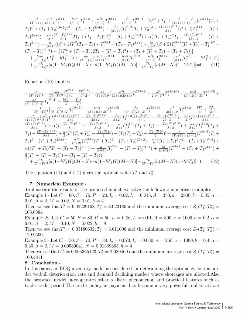
P 205International Journal on Current Science & Technology
Vol - I l No- I l January-June’2013
A deterministic inventory model.......... allowable shortage under trade credit 9
P(T1+T2)
[ αβ(β+1)
T β+1
1− bαβ
(β+1)T β+2
1+ α2b
(β+1)T 2β+2
1− α2
(β+1)T 2β+1
1− bT 2
1+T1]+
P(T1+T2)
[ α2
(β+1)(T β+1
1(T1+
T2)β + (T1 + T2)
β+1T β1− (T1 + T2)
2β+1)− α2b(β+2)
(T β+2
1(T1 + T2)
β + (T1+T2)β+1
β+1(β + 2)T β+1
1− (T1 +
T2)2β+2)− αb
2( (T1+T2)
β+1
β+12T1+(T1+T2)
βT 2
1− (T1+T2)
β+2)+α((T1+T2)βT1+
(T1+T2)β+1
(β+1)− (T1+
T2)β+1)− α
(β+1)((β+1)T β
1(T1+T2)+T β+1
1− (T1+T2)
β+1)+ bαβ+2
((β+2)T β+1
1(T1+T2)+T β+2
1−
(T1 + T2)β+2) + b
2(T 2
1+ (T1 + T2)2T1 − (T1 + T2)
2)− (T1 + (T1 + T2)− (T1 + T2))]
+ Caα(T1+T2)
(T β1− bT β+1
1) + ah
(T1+T2)[ αβ(β+1)
T β+1
1− bαβ
(β+1)T β+2
1+ α2b
(β+1)T 2β+2
1− α2
(β+1)T 2β+1
1− bT 2
1+ T1]
+ SIe(T1+T2)
2 [a(1−bT2)T2(M−N)+a(1−bT1)T1(M−N)]− SIe(T1+T2)
[a(M−N)(1−2bT1)]=0 (11)
Equation (10) implies
− A(T1+T2)
2 − Caα(T1+T2)
2 [Tβ+11
β+1− bTβ+2
1
β+2]− ah
(T1+T2)2 [
α2b(β+1)(2β+3)
T(2β+3)
1− α2
2(β+1)2T
(2β+2)
1− bαβ
(β+1)(β+3)T
(β+3)
1+
αβ(β+1)(β+2)
T(β+2)
1− bT 3
1
3+
T 21
2]
− P(T1+T2)
2 [αβ
(β+1)(β+2)T
(β+2)
1− bαβ
(β+1)(β+3)T
(β+3)
1+ α2b
(β+1)(2β+3)T
(2β+3)
1− α2
2(β+1)2T 2β+2
1− bT 3
1
3+
T 21
2]−
P(T1+T2)
2 [α2
β+1(T β+1
1
(T1+T2)β+1
β+1− (T1+T2)
2β+2
2β+2)− α2b
β+2(T β+2
1
(T1+T2)β+1
β+1− (T1+T2)
2β+3
2β+3)− αb
2(T 2
1
(T1+T2)β+1
β+1−
(T1+T2)β+3
β+3) + α(T1
(T1+T2)β+1
β+1− (T1+T2)
β+2
β+2) − α
β+1(T β+1
1(T1 + T2) − (T1+T2)
β+2
β+2) + bα
β+2(T β+2
1(T1 +
T2)− (T1+T2)β+3
β+3)+ b
2(T 2
1(T1+T2)− (T1+T3)
3
3)− (T1(T1+T2)− (T1+T2)
2
2)]+ P
(T1+T2)[ α2
(β+1)(T β+1
1(T1+
T2)β− (T1+T2)
2β+1)− α2b(β+2)
(T β+2
1(T1+T2)
β− (T1+T2)2β+2)− αb
2((T1+T2)
βT 2
1− (T1+T2)
β+2)+
α((T1 + T2)βT1 − (T1 + T2)
β+1) − α(β+1)
(T β+1
1− (T1 + T2)
β+1) + bα(β+2)
(T β+2
1− (T1 + T2)
β+2) +b2(T 2
1− (T1 + T2)
2)− (T1 − (T1 + T2))]
+ SIe(T1+T2)
2 [a(1−bT2)T2(M−N)+a(1−bT1)T1(M−N)]− SIe(T1+T2)
[a(M−N)(1−2bT2)]=0 (12)
The equation (11) and (12) gives the optimal value T ∗1and T ∗
2.
7. Numerical Example:-To illustrate the results of the proposed model, we solve the following numerical examples.Example 1:- Let C = 60, S = 70, P = 20, Ic = 0.02, Ie = 0.015, A = 350, a = 2900, b = 0.35, α =0.01, β = 2,M = 0.02, N = 0.01, h = 4Then we see thatT ∗
1= 0.02229108, T ∗
2= 8.023180 and the minimum average cost Z1(T
∗1, T ∗
2) =
103.6384Example 2:- Let C = 50, S = 80, P = 50, Ic = 0.06, Ie = 0.01, A = 300, a = 1000, b = 0.2, α =0.01, β = 2,M = 0.10, N = 0.022, h = 8Then we see thatT ∗
1= 0.03180632, T ∗
2= 3.611006 and the minimum average cost Z2(T
∗1, T ∗
2) =
129.9500Example 3:- Let C = 50, S = 70, P = 30, Ic = 0.070, Ie = 0.030, A = 250, a = 1000, b = 0.4, α =0.30, β = 2,M = 0.09589041, N = 0.01369863, h = 4Then we see thatT ∗
1= 0.005365123, T ∗
2= 2.080469 and the minimum average cost Z1(T
∗1, T ∗
2) =
100.48118. Conclusion:-In this paper, an EOQ inventory model is considered for determining the optimal cycle time un-der weibull deterioration rate and demand declining market where shortages are allowed.Alsothe proposed model in-cooperates other realistic phenomenon and practical features such astrade credit period.The credit policy in payment has become a very powerful tool to attract

P 206International Journal on Current Science & Technology Vol - I l No- I l January-June’2013
10 Pinki Majumder and U.K.Bera
new customers and a good incentive policy for the buyers.In keeping with this reality , thesefactors are incorporated into the present model. Numerical examples are presented to justifythe claim of each case of the model analysis by obtaining the optimal inventory length, shortagetime period and also calculated the total variable cost.The proposed model can be extended in several ways.For instance,we may extend this modelfor partial trade credit period, quantity discount,taking selling price, ordering cost , demandas a fuzzy number.
9. References:-
[1]Covert R.P and Philip G. C(1973),An EOQ model for items with weibull distribution de-terioration ,AIIE Transactions,5,323-326.
[2]Chen L.H,Ouyang L.Y.,Fuzzy inventory model for deteriorating items with permissibledelay in payment,Appl. Math. Comput. 182(2006)711-726.
[3] Chen L.H ,Kang F.S (2010),Integrated inventory models considering permissible delay inpayment and variant pricing strategy , Appl. Math. Model,34,36-46.
[4] Chen M.L and Chang M. C. (2011),Optimal order quantity under advance sales and per-missible delays in payment,African Journal of Business Management 5(17),7325-7334.
[5] Deb m. and Chaudhuri K.S.(1986), An EOQ Model for items with finite rate of produc-tion and variable rate of deterioration, Opsearch,23,175-181.
[6]Goyal S.K,Economic order quantity under conditions of permissible delay in payments,J.Operat. Res.Soc. 36(1985) 335-338.
[7]Jamal A.M.M , Sarker B.R,Wang S.,An ordering policy for deteriorating items with al-lowable Shortage and permissible delay in payment .Journal of Operation Research society48(1997) 826-833.
[8] Kumar M., Tripathi R.P. and Singh S.R (2008) , Optimal ordering policy and pricingwith variable demand rate under trade credits,Journal of National Academy of Mathematics ,22,111-123.
[[9] Meher M. K , Panda G.C, Sahu S.K ,An Inventory Model with weibull DeteriorationRate under the Delay in payment in Demand Declining Market , Applied Mathematical sci-ences, vol.6,2012 no. 23,1121-1133.
[10] Shah Y.K and Jaiswal M.C (1977) ,An order-level inventory Model for a system withconstant rate of deterioration , Opsearch 14, 174-184.
[11] Sarker B. R , Jamal A.M.M ,Wang S., Supply chain models for perishable products underinflation and permissible delay in payment.Computational Operation Research 27 (2000) 59-75.
DEVELOPMENT OF LABVIEW BASED ELECTRONIC NOSE USING K-NN ALGORITHM FOR THE DETECTION AND
CLASSIFICATION OF FRUITY ODORS
ABSTRACT
The basic objective of this paper is to development of electronic nose system which can able to detect and classify different fruits basing upon their odor with help of LabVIEW. This system consists of two Figaro gas sensors (TGS 2620 and TGS 2602) which is used detection for odor and k-NN Algorithm is used to classify different fruits.
Olfaction is one’s sense of smell and a primary human sensory system. The detection of odors has been applied to many industrial applications, including indoor air quality, health care, safety and security, environmental monitoring, quality control of food products, medical diagnosis, psychoanalysis, agriculture, pharmaceuticals, military applications, and detection of hazardous gases, to name but a few. The biological nose is an obvious choice for such applications, but there are some disadvantages to having human beings perform these tasks because they have to face various difficulties such as fatigue, infections, mental state, subjectivity, exposure to hazardous materials etc., due to above reasons machines are preferred to do the above applications which show high accuracy then human beings.
Keywords : Electronic nose, Virtual Instrumentation, K-NN algorithm, Fruity Odors
I. NTRODUCTION
An electronic nose is a device intended to detect odors or flavors. The expression electronic sensing refers to the capability of reproducing human senses using sensor arrays and pattern recognition systems. Since 1982 research has been conducted to develop technologies[2], commonly referred to as electronic noses that could detect and recognize odors and flavors. The stages of the recognition process are similar to human olfaction and are performed for identification, comparison, quantification and other applications, including data storage and retrieval. These devices have undergone
N.Jagadesh babu
Assistant professor, EIE Department,Gitam University, Visakhaptanam,A.P,India.
E-mail : [email protected]
much development and are now used to fulfill industrial needs.
Other techniques to analyze odorsIn all industries, odor assessment is usually performed by human sensory analysis, by chemo sensors, or by gas chromatography. The latter technique gives information about volatile organic compounds but the correlation between analytical results and actual odor perception is not direct due to potential interactions between several odorous components.
Working principleThe electronic nose was developed in order to mimic human olfaction that functions as a non-separative mechanism: i.e. an odor or flavor is perceived as a global fingerprint. Essentially the instrument consists of head space sampling, sensor array, and pattern recognition modules, to generate signal pattern that are used for characterizing odors. Electronic noses include three major parts: A sample delivery system, A detection system and A computing system.
Detection System: This consists of a sensor set, is the reactive part of the instrument. When in contact with volatile compounds, the sensors react, which means they experience a change of electrical properties. Each sensor is sensitive to all volatile molecules but each in their specific way. Most electronic noses use sensor arrays that react to volatile compounds on contact: the adsorption of volatile compounds on the sensor surface causes a physical change of the sensor. A specific response is recorded by the electronic interface transforming the signal into a digital value. Recorded data are then computed based on statistical models.The more commonly used sensors include:Computing System:They work to combine the responses of all of the sensors, which represent the input for the data treatment. This part of the instrument performs global fingerprint analysis and provides results and representations that can be easily
P 207International Journal on Current Science & Technology
Vol - I l No- I l January-June’2013
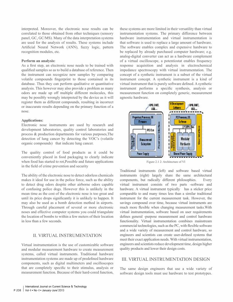
interpreted. Moreover, the electronic nose results can be correlated to those obtained from other techniques (sensory panel, GC, GC/MS). Many of the data interpretation systems are used for the analysis of results. These systems include Artificial Neural Network (ANN), fuzzy logic, pattern recognition modules, etc.
Perform an analysis:As a first step, an electronic nose needs to be trained with qualified samples so as to build a database of reference. Then the instrument can recognize new samples by comparing volatile compounds fingerprint to those contained in its database. Thus they can perform qualitative or quantitative analysis. This however may also provide a problem as many odors are made up off multiple different molecules, this may be possibly wrongly interpreted by the device as it will register them as different compounds, resulting in incorrect or inaccurate results depending on the primary function of a nose.
Applications:Electronic nose instruments are used by research and development laboratories, quality control laboratories and process & production departments for various purposes,The detection of lung cancer by detecting the VOC’s (volatile organic compounds) that indicate lung cancer.
The quality control of food products as it could be conveniently placed in food packaging to clearly indicate when food has started to rot,Possible and future applications in the field of crime prevention and security
The ability of the electronic nose to detect odorless chemicals makes it ideal for use in the police force, such as the ability to detect drug odors despite other airborne odors capable of confusing police dogs. However this is unlikely in the mean time as the cost of the electronic nose is too great and until its price drops significantly it is unlikely to happen. It may also be used as a bomb detection method in airports. Through careful placement of several or more electronic noses and effective computer systems you could triangulate the location of bombs to within a few meters of their location in less than a few seconds.
II. VIRTUAL INSTRUMENTATION
Virtual instrumentation is the use of customizable software and modular measurement hardware to create measurement systems, called virtual instruments. Traditional hardware instrumentation systems are made up of predefined hardware components, such as digital multimeters and oscilloscopes that are completely specific to their stimulus, analysis or measurement function. Because of their hard-cored function,
these systems are more limited in their versatility than virtual instrumentation systems. The primary difference between hardware instrumentation and virtual instrumentation is that software is used to replace a large amount of hardware. The software enables complex and expensive hardware to be replaced by already purchased computer hardware; e.g. analog-digital converter can act as a hardware complement of a virtual oscilloscope, a potentiostat enables frequency response acquisition and analysis in electrochemical impedance spectroscopy with virtual instrumentation. The concept of a synthetic instrument is a subset of the virtual instrument concept. A synthetic instrument is a kind of virtual instrument that is purely software defined. A synthetic instrument performs a specific synthesis, analysis or measurement function on completely generic, measurement agnostic hardware.
Figure 2.1 2: Architecture of VI
Traditional instruments (left) and software based virtual instruments (right) largely share the same architectural components, but radically different philosophies. Every virtual instrument consists of two parts -software and hardware. A virtual instrument typically has a sticker price comparable to and many times less than a similar traditional instrument for the current measurement task. However, the savings compound over time, because virtual instruments are much more flexible when changing measurement tasks.With virtual instrumentation, software based on user requirements defines general -purpose measurement and control hardware functionality. Virtual instrumentation combines mainstream commercial technologies, such as the PC, with flexible software and a wide variety of measurement and control hardware, so engineers and scientists can create user-defined systems that meet their exact application needs. With virtual instrumentation, engineers and scientists reduce development time, design higher quality products and lower their design costs.
III. VIRTUAL INSTRUMENTATION DESIGN
The same design engineers that use a wide variety of software design tools must use hardware to test prototypes.
P 208International Journal on Current Science & Technology Vol - I l No- I l January-June’2013
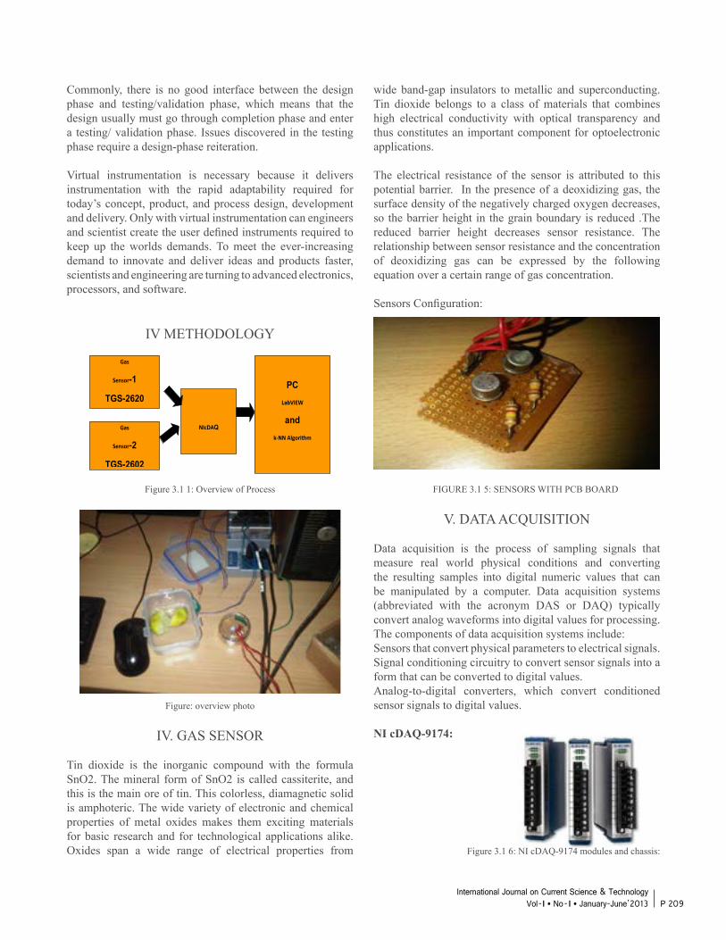
wide band-gap insulators to metallic and superconducting. Tin dioxide belongs to a class of materials that combines high electrical conductivity with optical transparency and thus constitutes an important component for optoelectronic applications.
The electrical resistance of the sensor is attributed to this potential barrier. In the presence of a deoxidizing gas, the surface density of the negatively charged oxygen decreases, so the barrier height in the grain boundary is reduced .The reduced barrier height decreases sensor resistance. The relationship between sensor resistance and the concentration of deoxidizing gas can be expressed by the following equation over a certain range of gas concentration.
Sensors Configuration:
FIGURE 3.1 5: SENSORS WITH PCB BOARD
V. DATA ACQUISITION
Data acquisition is the process of sampling signals that measure real world physical conditions and converting the resulting samples into digital numeric values that can be manipulated by a computer. Data acquisition systems (abbreviated with the acronym DAS or DAQ) typically convert analog waveforms into digital values for processing. The components of data acquisition systems include:Sensors that convert physical parameters to electrical signals.Signal conditioning circuitry to convert sensor signals into a form that can be converted to digital values.Analog-to-digital converters, which convert conditioned sensor signals to digital values.
NI cDAQ-9174:
Figure 3.1 6: NI cDAQ-9174 modules and chassis:
Commonly, there is no good interface between the design phase and testing/validation phase, which means that the design usually must go through completion phase and enter a testing/ validation phase. Issues discovered in the testing phase require a design-phase reiteration.
Virtual instrumentation is necessary because it delivers instrumentation with the rapid adaptability required for today’s concept, product, and process design, development and delivery. Only with virtual instrumentation can engineers and scientist create the user defined instruments required to keep up the worlds demands. To meet the ever-increasing demand to innovate and deliver ideas and products faster, scientists and engineering are turning to advanced electronics, processors, and software.
IV METHODOLOGY
Figure 3.1 1: Overview of Process
Figure: overview photo
IV. GAS SENSOR
Tin dioxide is the inorganic compound with the formula SnO2. The mineral form of SnO2 is called cassiterite, and this is the main ore of tin. This colorless, diamagnetic solid is amphoteric. The wide variety of electronic and chemical properties of metal oxides makes them exciting materials for basic research and for technological applications alike. Oxides span a wide range of electrical properties from
Gas
Sensor-1
TGS-2620
Gas
Sensor-2
TGS-2602
NIcDAQ
PC LabVIEW
and k-NN Algorithm
P 209International Journal on Current Science & Technology
Vol - I l No- I l January-June’2013
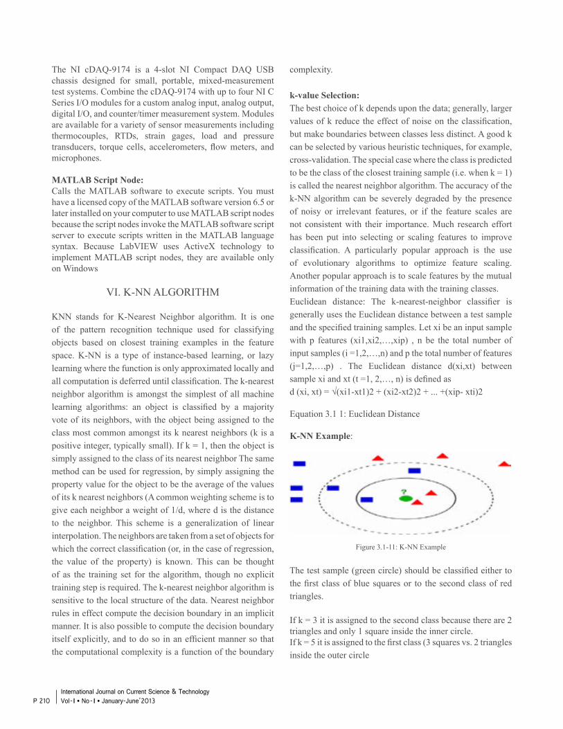
The NI cDAQ-9174 is a 4-slot NI Compact DAQ USB chassis designed for small, portable, mixed-measurement test systems. Combine the cDAQ-9174 with up to four NI C Series I/O modules for a custom analog input, analog output, digital I/O, and counter/timer measurement system. Modules are available for a variety of sensor measurements including thermocouples, RTDs, strain gages, load and pressure transducers, torque cells, accelerometers, flow meters, and microphones.
MATLAB Script Node:Calls the MATLAB software to execute scripts. You must have a licensed copy of the MATLAB software version 6.5 or later installed on your computer to use MATLAB script nodes because the script nodes invoke the MATLAB software script server to execute scripts written in the MATLAB language syntax. Because LabVIEW uses ActiveX technology to implement MATLAB script nodes, they are available only on Windows
VI. K-NN ALGORITHM
KNN stands for K-Nearest Neighbor algorithm. It is one of the pattern recognition technique used for classifying objects based on closest training examples in the feature space. K-NN is a type of instance-based learning, or lazy learning where the function is only approximated locally and all computation is deferred until classification. The k-nearest neighbor algorithm is amongst the simplest of all machine learning algorithms: an object is classified by a majority vote of its neighbors, with the object being assigned to the class most common amongst its k nearest neighbors (k is a positive integer, typically small). If k = 1, then the object is simply assigned to the class of its nearest neighbor The same method can be used for regression, by simply assigning the property value for the object to be the average of the values of its k nearest neighbors (A common weighting scheme is to give each neighbor a weight of 1/d, where d is the distance to the neighbor. This scheme is a generalization of linear interpolation. The neighbors are taken from a set of objects for which the correct classification (or, in the case of regression, the value of the property) is known. This can be thought of as the training set for the algorithm, though no explicit training step is required. The k-nearest neighbor algorithm is sensitive to the local structure of the data. Nearest neighbor rules in effect compute the decision boundary in an implicit manner. It is also possible to compute the decision boundary itself explicitly, and to do so in an efficient manner so that the computational complexity is a function of the boundary
complexity.
k-value Selection:The best choice of k depends upon the data; generally, larger values of k reduce the effect of noise on the classification, but make boundaries between classes less distinct. A good k can be selected by various heuristic techniques, for example, cross-validation. The special case where the class is predicted to be the class of the closest training sample (i.e. when k = 1) is called the nearest neighbor algorithm. The accuracy of the k-NN algorithm can be severely degraded by the presence of noisy or irrelevant features, or if the feature scales are not consistent with their importance. Much research effort has been put into selecting or scaling features to improve classification. A particularly popular approach is the use of evolutionary algorithms to optimize feature scaling. Another popular approach is to scale features by the mutual information of the training data with the training classes. Euclidean distance: The k-nearest-neighbor classifier is generally uses the Euclidean distance between a test sample and the specified training samples. Let xi be an input sample with p features (xi1,xi2,…,xip) , n be the total number of input samples (i =1,2,…,n) and p the total number of features (j=1,2,…,p) . The Euclidean distance d(xi,xt) between sample xi and xt (t =1, 2,…, n) is defined asd (xi, xt) = √(xi1-xt1)2 + (xi2-xt2)2 + ... +(xip- xti)2
Equation 3.1 1: Euclidean Distance
K-NN Example:
Figure 3.1-11: K-NN Example
The test sample (green circle) should be classified either to the first class of blue squares or to the second class of red triangles.
If k = 3 it is assigned to the second class because there are 2 triangles and only 1 square inside the inner circle. If k = 5 it is assigned to the first class (3 squares vs. 2 triangles inside the outer circle
P 210International Journal on Current Science & Technology Vol - I l No- I l January-June’2013
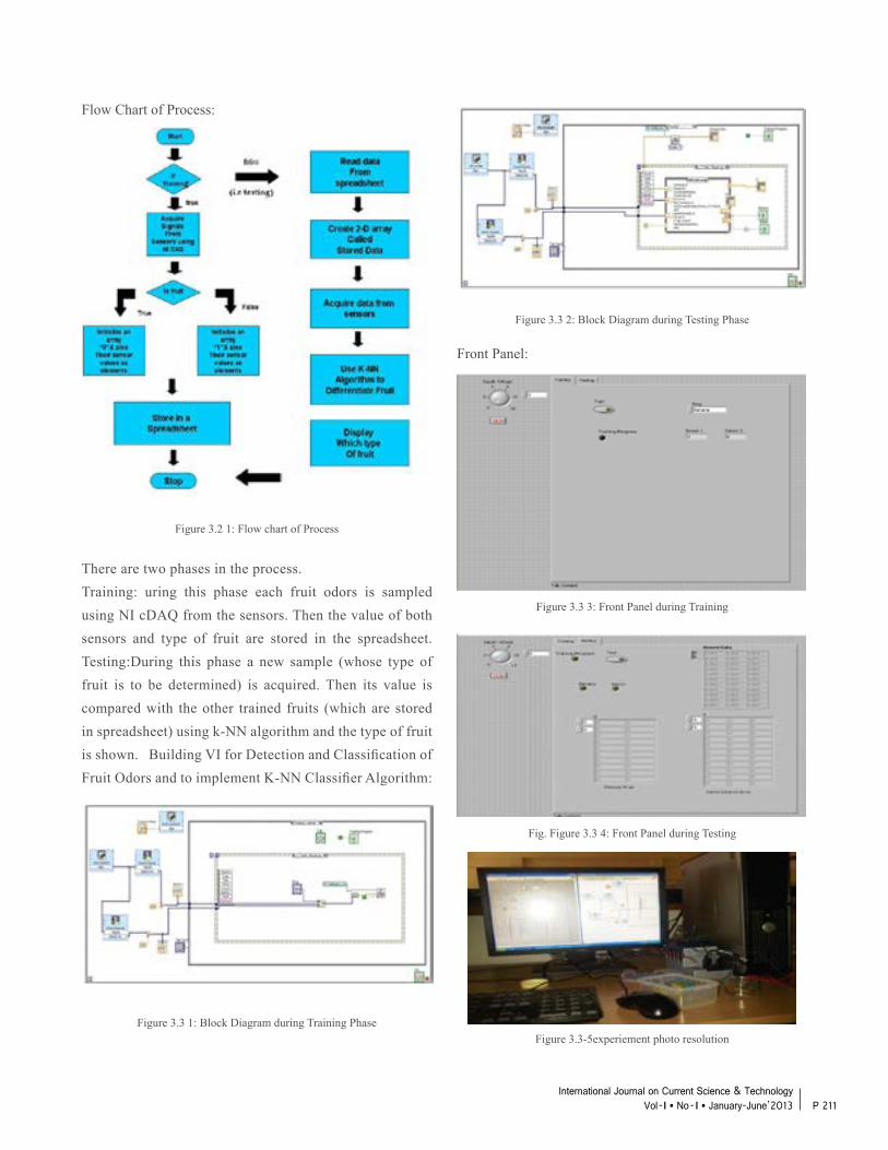
Flow Chart of Process:
Figure 3.2 1: Flow chart of Process
There are two phases in the process. Training: uring this phase each fruit odors is sampled using NI cDAQ from the sensors. Then the value of both sensors and type of fruit are stored in the spreadsheet.Testing:During this phase a new sample (whose type of fruit is to be determined) is acquired. Then its value is compared with the other trained fruits (which are stored in spreadsheet) using k-NN algorithm and the type of fruit is shown. Building VI for Detection and Classification of Fruit Odors and to implement K-NN Classifier Algorithm:
Figure 3.3 1: Block Diagram during Training Phase
Figure 3.3 2: Block Diagram during Testing Phase
Front Panel:
Figure 3.3 3: Front Panel during Training
Fig. Figure 3.3 4: Front Panel during Testing
Figure 3.3-5experiement photo resolution
P 211International Journal on Current Science & Technology
Vol - I l No- I l January-June’2013
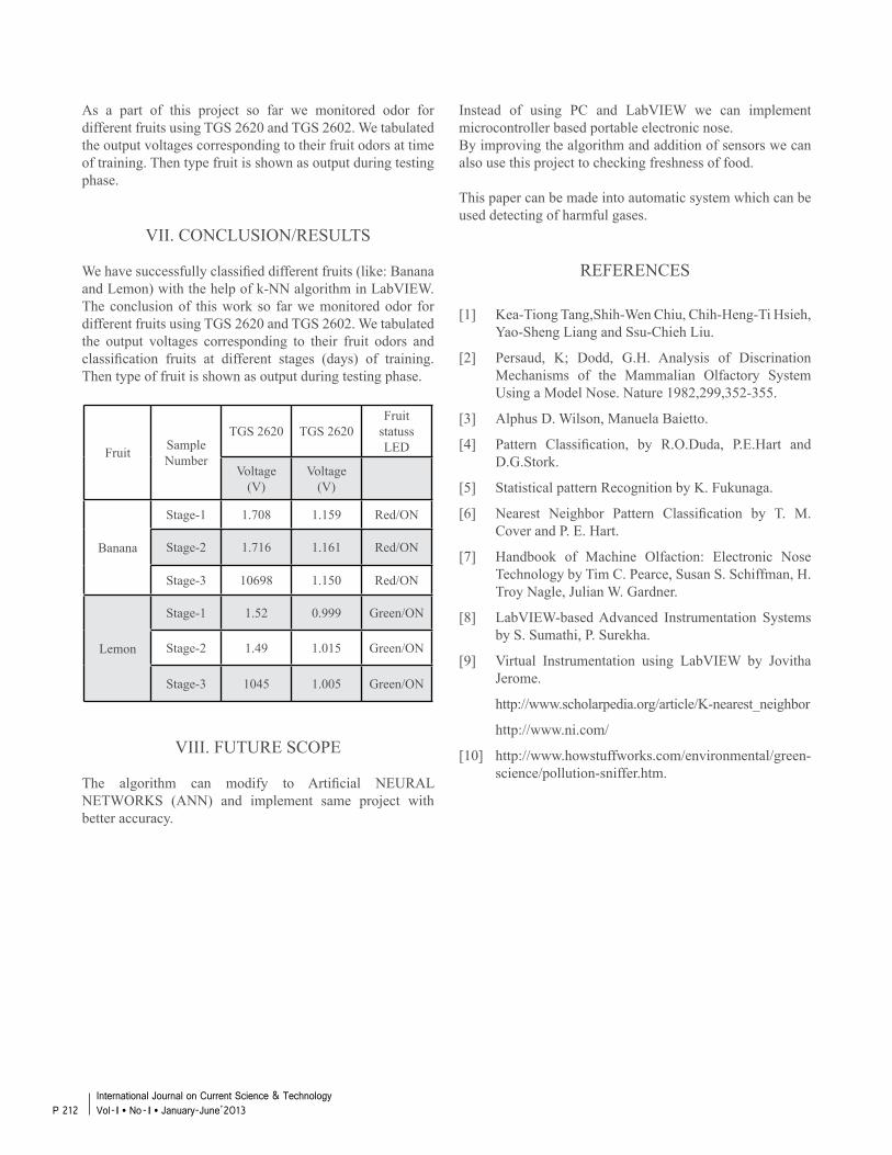
As a part of this project so far we monitored odor for different fruits using TGS 2620 and TGS 2602. We tabulated the output voltages corresponding to their fruit odors at time of training. Then type fruit is shown as output during testing phase.
VII. CONCLUSION/RESULTS
We have successfully classified different fruits (like: Banana and Lemon) with the help of k-NN algorithm in LabVIEW. The conclusion of this work so far we monitored odor for different fruits using TGS 2620 and TGS 2602. We tabulated the output voltages corresponding to their fruit odors and classification fruits at different stages (days) of training. Then type of fruit is shown as output during testing phase.
Fruit Sample Number
TGS 2620 TGS 2620Fruit
statuss LED
Voltage (V)
Voltage (V)
Banana
Stage-1 1.708 1.159 Red/ON
Stage-2 1.716 1.161 Red/ON
Stage-3 10698 1.150 Red/ON
Lemon
Stage-1 1.52 0.999 Green/ON
Stage-2 1.49 1.015 Green/ON
Stage-3 1045 1.005 Green/ON
VIII. FUTURE SCOPE
The algorithm can modify to Artificial NEURAL NETWORKS (ANN) and implement same project with better accuracy.
Instead of using PC and LabVIEW we can implement microcontroller based portable electronic nose.By improving the algorithm and addition of sensors we can also use this project to checking freshness of food.
This paper can be made into automatic system which can be used detecting of harmful gases.
REFERENCES
[1] Kea-Tiong Tang,Shih-Wen Chiu, Chih-Heng-Ti Hsieh, Yao-Sheng Liang and Ssu-Chieh Liu.
[2] Persaud, K; Dodd, G.H. Analysis of Discrination Mechanisms of the Mammalian Olfactory System Using a Model Nose. Nature 1982,299,352-355.
[3] Alphus D. Wilson, Manuela Baietto.
[4] Pattern Classification, by R.O.Duda, P.E.Hart and D.G.Stork.
[5] Statistical pattern Recognition by K. Fukunaga.
[6] Nearest Neighbor Pattern Classification by T. M. Cover and P. E. Hart.
[7] Handbook of Machine Olfaction: Electronic Nose Technology by Tim C. Pearce, Susan S. Schiffman, H. Troy Nagle, Julian W. Gardner.
[8] LabVIEW-based Advanced Instrumentation Systems by S. Sumathi, P. Surekha.
[9] Virtual Instrumentation using LabVIEW by Jovitha Jerome.
http://www.scholarpedia.org/article/K-nearest_neighbor
http://www.ni.com/
[10] http://www.howstuffworks.com/environmental/green- science/pollution-sniffer.htm.
P 212International Journal on Current Science & Technology Vol - I l No- I l January-June’2013

Annual Subscription In Rupees In US$International Journal on Current Science &
TechnologyRs. 5000/- US$100
Payable by Bank Transfer/RTGS to Account No. 32709506720, Name of the bank Nirjuli, Bank code 9535, IFS Code: SBIN0009535. Once paid details of Postal address of subscriber and scanned copy of Bank receipt may be send by E-mail to [email protected]
Authors’ Instruction
The papers on the following subjects should reach in IEEE format only by E-mail : [email protected]/[email protected] and a hard copy by post.
To, The Editor,International Journal on Current Science & Technology,National Institute of Technology - Arunachal Pradesh PO - Yupia, P.S. - Doimukh, Dist. - Papum Pare,Pin - 791112, Arunachal Pradesh
Acceptance of paper is based on peer-review process.Technical Education, Chemical Sciences, Engineering Sciences, Environmental Sciences, Information and communication Science & Technology (including Computer Sciences), Material Sciences, Mathematical Sciences (including Statistics), Medical Sciences, New Biology (including Biochemistry, Biophysics & Molecular Biology and Biotechnology) and Physical Sciences.
SUBSCRIPTION RATE
P 213International Journal on Current Science & Technology
Vol - I l No- I l January-June’2013

P 214International Journal on Current Science & Technology Vol - I l No- I l January-June’2013

P 215International Journal on Current Science & Technology
Vol - I l No- I l January-June’2013

National Instiute Of Technology Arunachal Pradesh(Estd. By MHRD, Govt. of India)
PO-Yupia, P.O.-Doimukh, Dist-Papum Pare, Pin-791112, Arunachal Pradesh
T 0360-2284801, F 0360-2284972
E [email protected]; [email protected]
International Journal on Current Science & TechnologyVol. : 1 | No. : 1 | January - June’ 2013
For Correspondence
ISSN : 2320 5636