Impact of Improved Maize Variety Adoption on Household Food Security in Ethiopia: An

Endogenous Switching Regression Approach

Moti Jaleta1, Menale Kassie2, and Paswel Marenya1

1International Maize and Wheat Improvement Center (CIMMYT), Addis Ababa, Ethiopia

2 CIMMYT, Nairobi, Kenya

Abstract

This paper analyzes the adoption and impacts of improved maize varieties (IMVs) on food security

in Ethiopia. Survey data collected in 2011 from 2455 sample households in 39 districts was used in

the analysis. Endogenous switching regression model supported by binary and generalized

propensity score matching methods was used to empirically assess the impact of IMV adoption on

per-capita food consumption expenditure and perceived household food security status. Results

show that education of household head, farm size, social network, and better agro-ecologic

potential for maize production are the major determinants of household decisions to adopt IMVs. In

addition, the average per-capita food consumption is high for adopters and the impact of IMV

adoption on per-capita food consumption is slightly higher for non-adopters had they adopted

IMVs. Thus, policies and development strategies encouraging further adoption of IMVs could

enhance food security of smallholder farmers in maize-based systems.

Keywords: Improved maize, adoption, impact, endogenous switching regression, smallholder,

Ethiopia.

JEL codes: C31, C34, D6, D13

2

1. Introduction

Food security is one of the major challenges the World has been fighting for long. The

prevalence of food security problem in regions with increasing population growth and more

exposed to agonies of climate change makes the challenge rather complex and put more people

under malnutrition (Parry et al., 1999; Brown et al., 2008; Godfray et al., 2010; Beddington,

2010). Recent data show that close to 0.8 billion people in the World are undernourished. About

28% of this are living in sub-Saharan Africa and of which more than half are living in East

Africa (FAO, 2015).

In the region, Ethiopia is one of the countries strongly associated with prolonged food security

problem and recently set a clear agricultural production and productivity development policy to

tackle the challenge and lift millions of smallholder farmers out of the food insecurity trap. This

has been supported by research and extension endeavors particularly on improving the

production and productivity of major staple crops widely grown by resource poor smallholder

farmers. In this regard, effort that has been made on maize research and extension is a good

example.

In Ethiopia, maize is widely produced and consumed by smallholder farmers. It is the major

staple crop leading all other cereals in terms of production and productivity, and only surpassed

by tef 1in terms of area (CSA, 2014a). As a strategic food security crop, since 1970s,

international and national research centers exerted collaborative efforts in improving the genetic

potential of maize and its adaptability to different agro-ecologies in the country. Through this

integrated effort, about 60 improved maize varieties have been released or registered in the

country since the 1970s (MoA, 2012). Except in both extreme lowlands and highlands, maize is

adapted to and grown in diverse agro-ecologies starting from mid-lowlands to highlands of the

country.

Although a large number of maize varieties have been released, the level of improved maize

variety adoption by smallholder farmers is still low (Feleke and Zegeye, 2006; Tura et al., 2010;

Kassa et al., 2013). For smallholder farmers in maize-based systems, maize is directly associated

1

Tef is an endemic and fine-grained cereal crop widely grown in Ethiopia.

3

with their food security. On average, 76% percent of maize produced is consumed at home

(CSA, 2014b). No other cereal crop produced reaches to this level in terms of retention for home

consumption. Thus, for smallholder farmers in maize-based systems, their perception on own-

food security status is directly related to the amount of maize harvest they produced in a given

year, which is again related to maize productivity influenced by factors such as varieties used

and crop management efforts put forth.

The main objective of this paper is to assess the impact of improved maize variety adoption on

food security of maize growing smallholder farmers using both objective and subjective

assessment outcomes, i.e., per-capita food consumption expenditure and self-perceived and

reported household food security status, respectively.

The remaining part of the paper is structured as follows. Section 2 presents survey design and

data used in the analysis. Methodological framework is discussed in section 3. Section 4

discusses both descriptive and empirical analysis results and section 5 concludes the paper.

2. Survey Design and Data

The cross sectional data used in this analysis came from a stratified random sample of 2455 farm

households from 39 districts in five regional states of Ethiopia (Tigray, Amhara, Oromia,

Benishangul-Gumuz, and SNNPR2). First, a list of 118 maize growing districts was obtained

from the CSA/IFPRI 2002 dataset that contained both the production data and area under maize

in each district level. The CSA/IFPRI 2002 data showed that an average maize productivity of

2.051 tons/ha with a standard deviation of 0.648. Based on these values, we assigned a mean ±

standard deviation cut-off points to categorize the districts in to a ‘high’, ‘medium’, and ‘low’

maize potential. Accordingly, districts with average maize productivity of less than 1.403 tons/ha

were assigned as ‘low potential’, above 2.698 tons/ha as ‘high potential’, and between 1.403 and

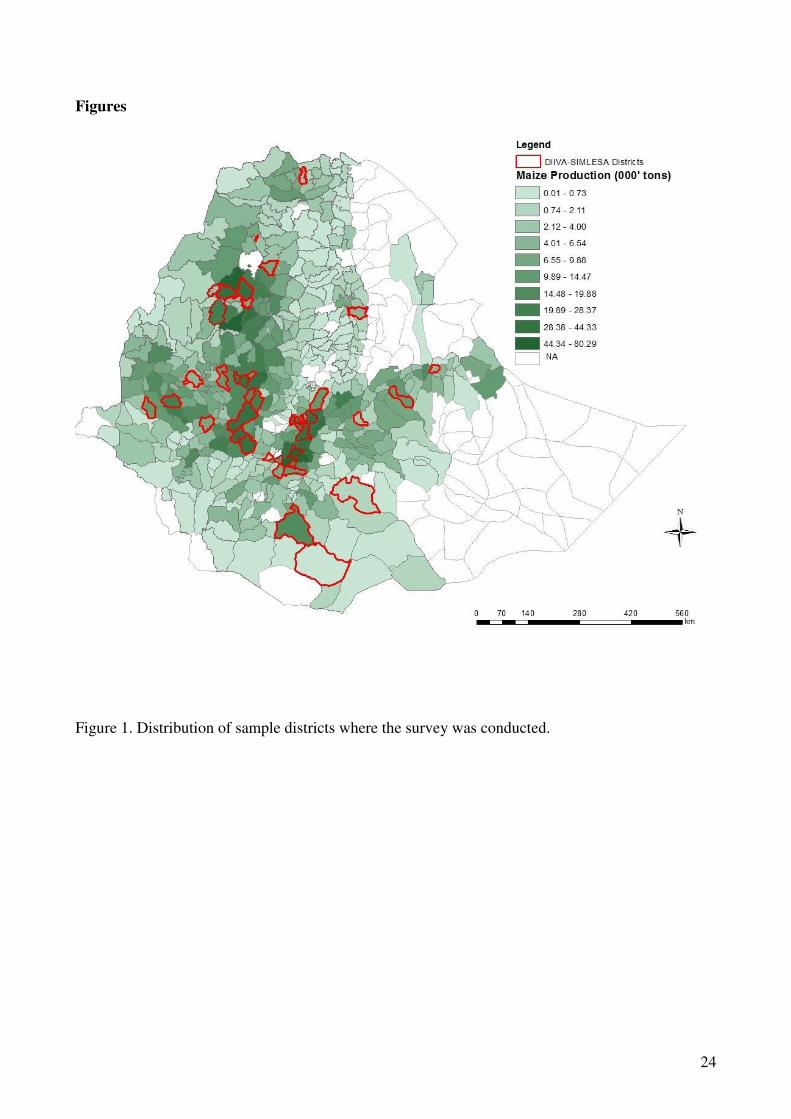
2.698 tons/ha (both inclusive) as ‘medium potential’ maize districts. We then selected 39 districts

(slightly above 30% of the districts listed in the sampling frame) using a proportionate

probability sampling method. Geographical locations of the sample districts and the maize

production potential of each district are given in Figure 1.

2

Southern Nations, Nationalities and Peoples Regional State.

4

< Figure 1 here >

In each selected district, 4 peasant associations (PAs) were randomly selected from maize

growing PAs and in each PA, an average of 10-16 farmers were randomly selected for one-to-

one interviews. This resulted in a sample of 603 households from the high potential districts,

1528 and 324 from the medium and low potential districts respectively (Table 1).

< Table 1 here >

The household level survey was conducted on one-to-one basis using experienced and trained

enumerators. The overall fieldwork was closely monitored and supervised by staff from the

Ethiopian Institute of Agricultural Research (EIAR) and the International Maize and Wheat

Improvement Center (CIMMYT).

A questionnaire was developed and tested to collect the adoption data. The questionnaire

captured individual, household, farm and plot level characteristics, as well as the institutional

environment. The individual characteristics included demographics such as age, gender, and

education of the head of the household, and his or her knowledge of different varieties.

Household characteristics included; resource endowments, farm and non-farm assets, and the use

of maize varieties. Institutional factors included access to markets, institutions and infrastructure.

The characteristics of the different farm plots were also taken, in particular fertility, slope, soil

type, distance from homestead, manager of each plot from the household members, etc.), crops

grown on each plots including the detailed inputs used per plot, maize varieties grown per plot,

source of maize seed and number of years/seasons the maize seed used was recycled, production

and marketing constraints, and so forth. The data were collected during January to June 2011 and

covered production and input use for the 2009/10 production seasons.

3. Methodological Framework

In this paper, we used combinations of methodologies to ensure robustness of empirical results.

To determine factors affecting the adoption of improved maize varieties, a binary Probit model

was used. An endogenously switching regression (ESR) model and a propensity score matching

5

(PSM) method were used to estimate the effect of improved maize variety adoption on household

food security. The latter two methods are discussed below briefly.

3.1. Endogenous Switching Treatment Effect Regression Analysis

3.1.1. Econometric Model Specification

A survey of recent literature shows that many impact assessment studies based on cross-sectional

data have moved towards endogenously switching regression model (Alene and Manyong, 2007;

Amare et al., 2012; Asfaw et al., 2012; Kassie et al., 2014; Abdulai and Huffman, 2014; among

others) The assumption behind using endogenously switching treatment effect regression is that,

in addition to the observed variables, there might be unobservable farm and/or household

characteristics that could potentially influence both the adoption of improved maize varieties and

household food security. A farm household self-selects into adopting agricultural technologies

due to observable and unobservable variables. Estimating the impact of technology adoption on

household food security without accounting for this problem might suffer from potential

endogeneity bias and thus the estimated results may over- or under-estimate impacts compared to

the actual impact. To correct for this, endogenous switching regression analysis was used and

selectivity is modeled using a Probit model. The overall econometric modeling framework used

is described below.

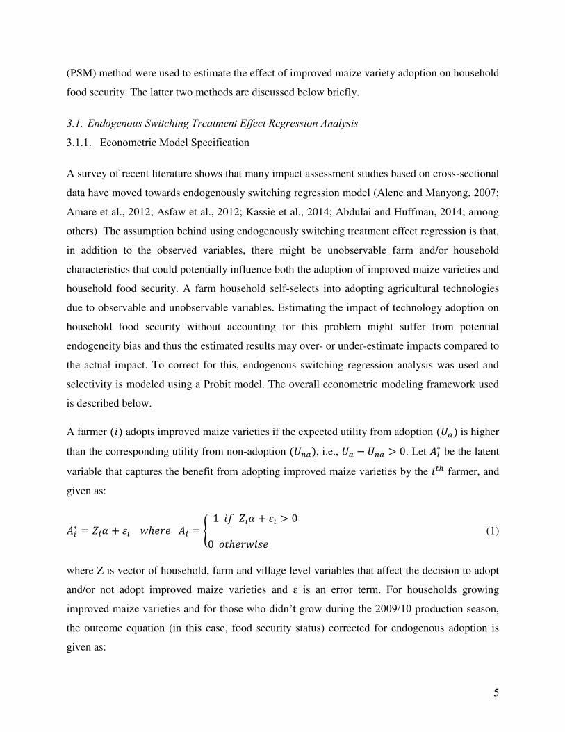
A farmer � adopts improved maize varieties if the expected utility from adoption � is higher

than the corresponding utility from non-adoption �� , i.e., � − �� > . Let �∗ be the latent

variable that captures the benefit from adopting improved maize varieties by the ��ℎ farmer, and

given as:

�∗ = � + �� �ℎ � = { � � + �� > ℎ �� (1)

where Z is vector of household, farm and village level variables that affect the decision to adopt

and/or not adopt improved maize varieties and ɛ is an error term. For households growing

improved maize varieties and for those who didn’t grow during the 2009/10 production season,

the outcome equation (in this case, food security status) corrected for endogenous adoption is

given as:

6

� � : � = � + � ��̂ � + � � � � = � (2a) � � : � = � + � ��̂ � + � � � � = − � (2b)

where � is a binary food security status of household � under regime 1 (adopter of IMV) and 2

(local maize varieties), � is a vector of plot, household, farm, and village characteristics that

affect maize productivity, and �̂ � = � ���̂Φ ���̂ and �̂ � = � ���̂1−Φ ���̂ are the inverse Mill’s ratios (IMR)

computed from the selection equation and are included in equations (2a) and (2b) to correct for

selection bias in a two-step estimation procedure, i.e., endogenous switching regression. and σ

are parameters to be estimated, and η is an independently and identically distributed error term.

The standard errors in equations (2a) and (2b) are bootstrapped to account for the

heteroskedasticity arising from the generated regressors (�̂). The adoption decision of improved maize variety could be endogenous in the outcome equation

(food security) and estimating the outcome variable without correcting for the potential

endogeneity could result into biased estimates. Thus, identification of the outcome equation from

the selection equation using an instrumental variables method is important. For the outcome

model to be identified, we used exclusion restrictions, where some variables affecting the

selection variable but not the outcome variable are excluded from the outcome equation (Di

Falco et al., 2011; Asfaw et al., 2012; Kassie et al., 2014; Shiferaw et al., 2014). Although we

admit that getting a true instrument is empirically challenging, we used distance to seed dealers

(walking minutes), number of traders known to farmer, and number of relatives (who could

provide support) in and outside village as instrumenting variables affecting the decision to adopt

IMV but not household food security. Using a falsification test, we checked the admissibility of

these instruments. A falsification test is a way of checking whether instrumental variables are

valid instruments if they affect the selection equation (adoption of IMV in our case) but not the

outcome variable (food security). Accordingly, the falsification test on the selected instrumental

variables shows that they jointly and statistically significantly affect the decision of IMV

adoption (in selection equation: Chi2=16.26; P-value=0.001) but not per-capita food

consumption expenditure and household food security status.

7

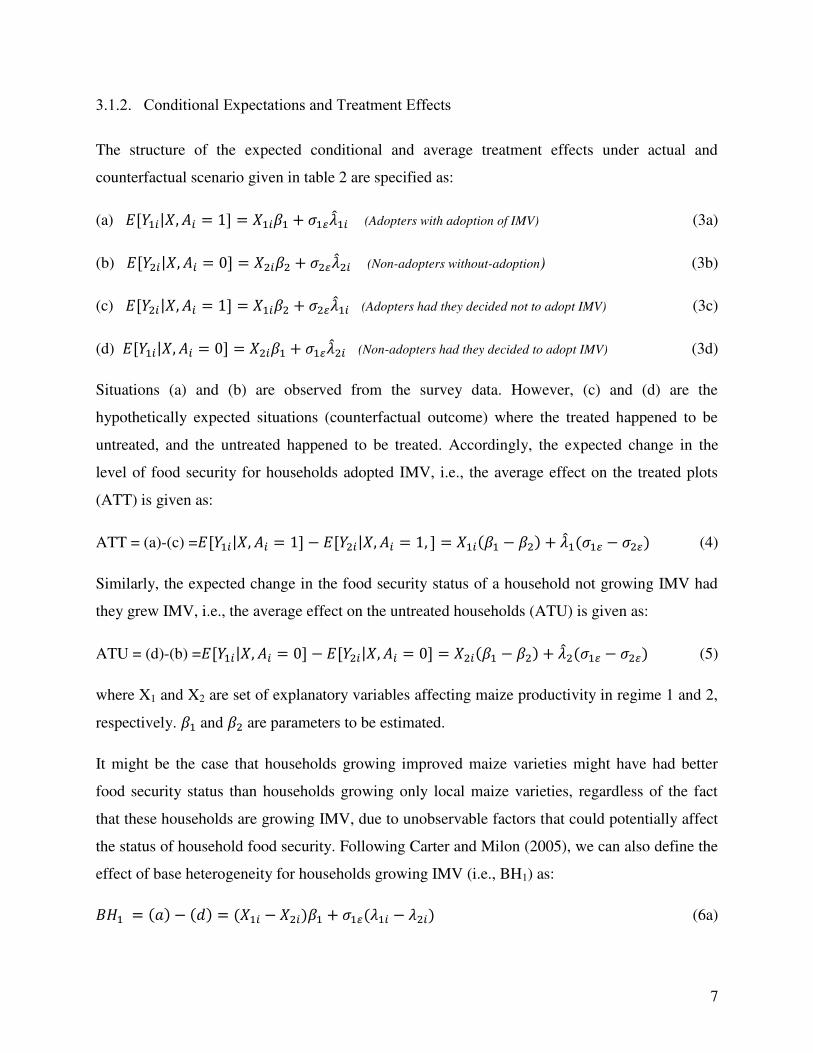
3.1.2. Conditional Expectations and Treatment Effects

The structure of the expected conditional and average treatment effects under actual and

counterfactual scenario given in table 2 are specified as:

(a) �[ �| , � = ] = � + � ��̂ � (Adopters with adoption of IMV) (3a)

(b) �[ �| , � = ] = � + � ��̂ � (Non-adopters without-adoption) (3b)

(c) �[ �| , � = ] = � + � ��̂ � (Adopters had they decided not to adopt IMV) (3c)

(d) �[ �| , � = ] = � + � ��̂ � (Non-adopters had they decided to adopt IMV) (3d)

Situations (a) and (b) are observed from the survey data. However, (c) and (d) are the

hypothetically expected situations (counterfactual outcome) where the treated happened to be

untreated, and the untreated happened to be treated. Accordingly, the expected change in the

level of food security for households adopted IMV, i.e., the average effect on the treated plots

(ATT) is given as:

ATT = (a)-(c) =�[ �| , � = ] − �[ �| , � = , ] = � − + �̂ � � − � � (4)

Similarly, the expected change in the food security status of a household not growing IMV had

they grew IMV, i.e., the average effect on the untreated households (ATU) is given as:

ATU = (d)-(b) =�[ �| , � = ] − �[ �| , � = ] = � − + �̂ � � − � � (5)

where X1 and X2 are set of explanatory variables affecting maize productivity in regime 1 and 2,

respectively. and are parameters to be estimated.

It might be the case that households growing improved maize varieties might have had better

food security status than households growing only local maize varieties, regardless of the fact

that these households are growing IMV, due to unobservable factors that could potentially affect

the status of household food security. Following Carter and Milon (2005), we can also define the

effect of base heterogeneity for households growing IMV (i.e., BH1) as: = − = � − � + � � � � − � � (6a)

8

Similarly, the base heterogeneity for maize plots under non-improved varieties (BH2) is given

as:

= − = � − � + � � � � − � � (6b)

Finally, transitional heterogeneity (TH) is explored by having a close look at whether the effect

of growing improved maize variety on household food security is larger for households that are

actually growing IMV than for households growing local varieties in the counterfactual case that

they would have been growing IMV, that is, the difference between equations (6a) and (6b) (i.e.,

TT and TU).

< Table 2 here >

3.2. Propensity Score Matching

In assessing the impacts of the treatment effect, getting proper counterfactuals from a cross-

sectional survey data is a challenge. Propensity score matching (PSM) helps in matching sample

households that fall into the treatment group with their proper counterfactuals (non-treatment

group but with attributes similar to the sample individuals under treatment group). In this paper,

the units to be matched are households growing IMV with their counterfactual households

growing only local varieties using three matching algorithms, viz., nearest neighbor, kernel and

radius matching methods. Whether the counterfactual households have the same characteristics

with the treatment group for observed variables are also tested. Finally, the average treatment

effect on the treated (ATT), i.e., the effect of IMV adoption on household level food security

status, is estimated based on the different matching methods indicated above. In addition, we

also used Generalized Propensity Score (GPS) approach to evaluate the effects of continuous

treatment (maize area under IMV) on the response of outcome variables, probability of food

security and per-capita expenditure on food consumption (Hirano and Imbens, 2004; Bia and

Mattei, 2007).

9

4. Results

4.1. Descriptive Analysis

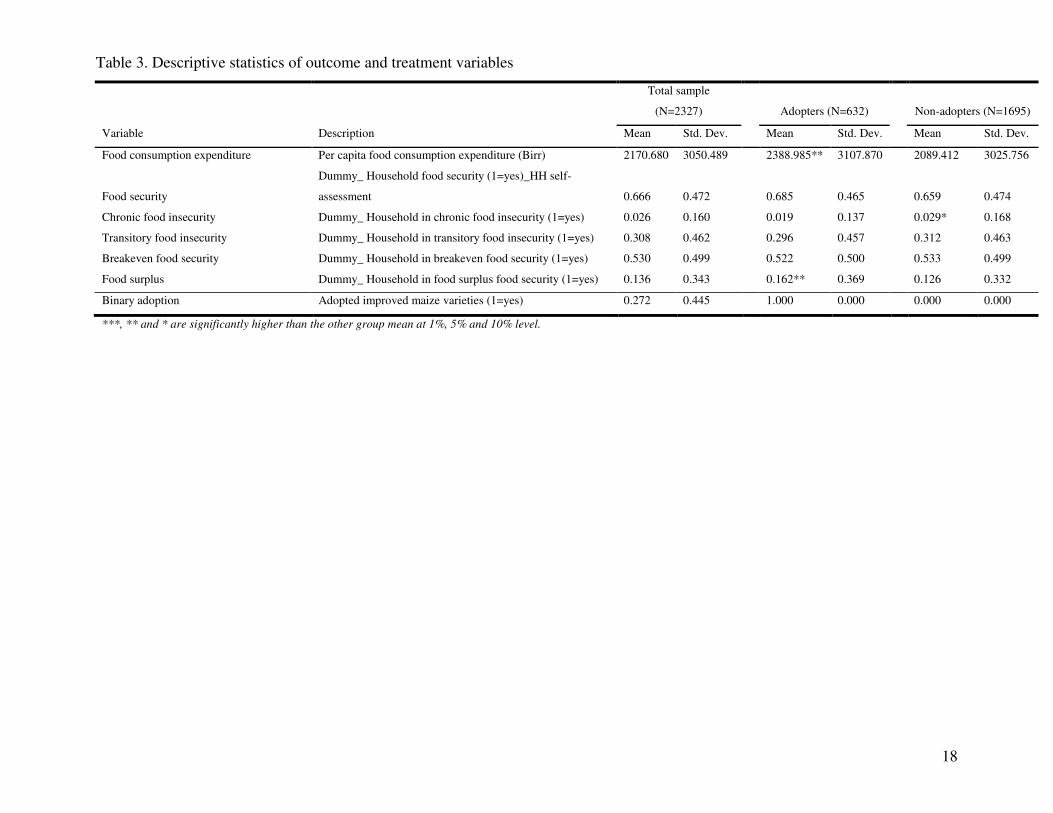
Descriptive analysis in table 3 shows that the average per-capita maize consumption, marketed

maize surplus, per capita food consumption expenditure and food security status are on the

higher side for adopters than non-adopter sample households. Looking more in depth at the

different cluster of adopter households divided in four groups depending on maize area allocated

to improved varieties, both the average per capita maize consumption and average quantity of

maize surplus sold to market are increasing with increasing area under improved maize. The

average per-capita food consumption expenditure is higher for lower middle quintile and the

proportion of sample households reported food security is high for upper middle quintile

households.

< Table 3 here >

The average per capita food consumption expenditure for the total sample households was ETB3

2170.68 ($127). However, compared to non-adopters, the average per capita food consumption

expenditure was higher for IMV adopters. Interestingly, looking at the binary food security

variable, there is no statistical difference between adopters and non-adopters in terms of the

proportion of households who self-reported as food secure. But, when we look at the four

clusters of food security (chronic, transitory, breakeven and food surplus), relatively a higher

proportion of non-adopter households reported as being under chronic food insecurity and a

larger proportion of adopters reported food surplus.

In table 4, descriptive statistics of explanatory variables used in adoption and impact analysis are

presented. Accordingly, the proportion of male headed households is higher for those who

adopted IMV. Non-adopter households relatively have older household heads with lower levels

of education. Average family size was higher for adopter households. IMV adoption was high in

high and medium maize potential areas. When adoption was categorized by the five

administrative regions, larger proportion of sample households were non-adopters in Oromia,

Benishangul Gumuz and Tigray regions whereas more proportion of sample households found to

3

ETB is Ethiopian Birr (Currency), where 1USD was equivalent to 17.01ETB during the survey period.

10

be adopters in Amhara and SNNPR. In general, adopter households know more number of

traders and have more social networks. Compered to non-adopters, adopter households has got

satisfied with their credit needs for fertilizer and improved seed purchases.

<Table 4 here >

4.2. Adoption of IMVs

Probit estimation results in table 5 show that household and farm characteristics, agro-ecologic

potential for maize production, and social capital had significant influence on farm household’s

decisions to adopt improved maize varieties. Farm households with more educated heads and

larger family size tend to adopt improved maize varieties. Compared to low potential areas for

maize production, the probability of IMV adoption is higher for maize growing households both

in high and medium potential areas. Controlling for diversities in maize potential, there is also a

difference in the probability of adoption across administrative regions. Compared to maize

growing households in the SNNPR, maize growing farmers in Amhara region have more

probability of adopting improved maize varieties. Unexpected results, which needs further

investigation is that the probability of adopting IMVs increases with increasing distance to the

main market and decreasing with increasing share of fertile plots a household owns.

<Table 5 here >

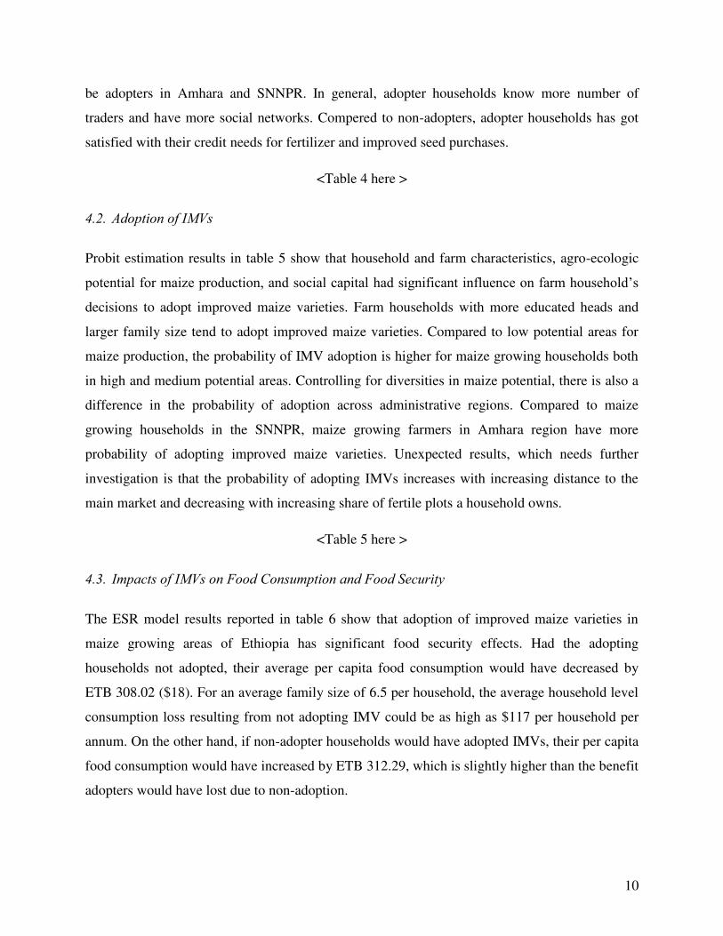
4.3. Impacts of IMVs on Food Consumption and Food Security

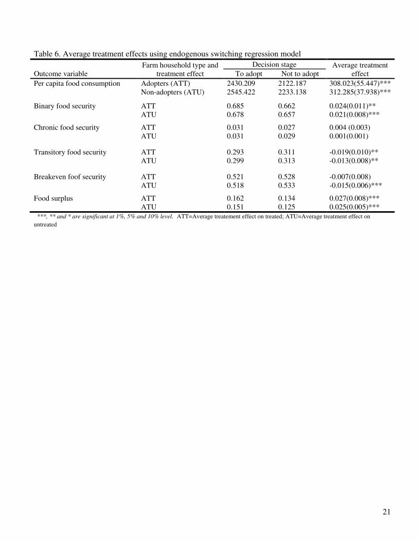
The ESR model results reported in table 6 show that adoption of improved maize varieties in

maize growing areas of Ethiopia has significant food security effects. Had the adopting

households not adopted, their average per capita food consumption would have decreased by

ETB 308.02 ($18). For an average family size of 6.5 per household, the average household level

consumption loss resulting from not adopting IMV could be as high as $117 per household per

annum. On the other hand, if non-adopter households would have adopted IMVs, their per capita

food consumption would have increased by ETB 312.29, which is slightly higher than the benefit

adopters would have lost due to non-adoption.

11

Looking into the binary food security variable, the average probability of being food secure

decreases by 2.4 percentage points for IMV adopters had they not adopted. In the same way, the

average probability of food security increases by 2.1 % point for non-adopters had they adopted

IMVs. A closer look at the the four categories of food security status showed that larger

probability differences are observed for households who reported that they were food secure. For

these sample farmers their average probability of being food surplus decreased by 2.7 percentage

points if they had not adopted IMVs and for non-adopters, their probability of being food surplus

increased by 2.5 percentage points had they adopted IMVs. These percentage points seem small

in magnitude but the difference is statistically significant at 1% level. As the main purpose of

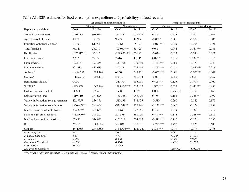
this paper is not to explain what factors affect the per-capita food consumption expenditure and

food security of maize producing households, the endogenously switching regression results used

as an intermediate input to estimate ATT and ATU are not discussed but presented in table A1 as

annex.

< Table 6 here >

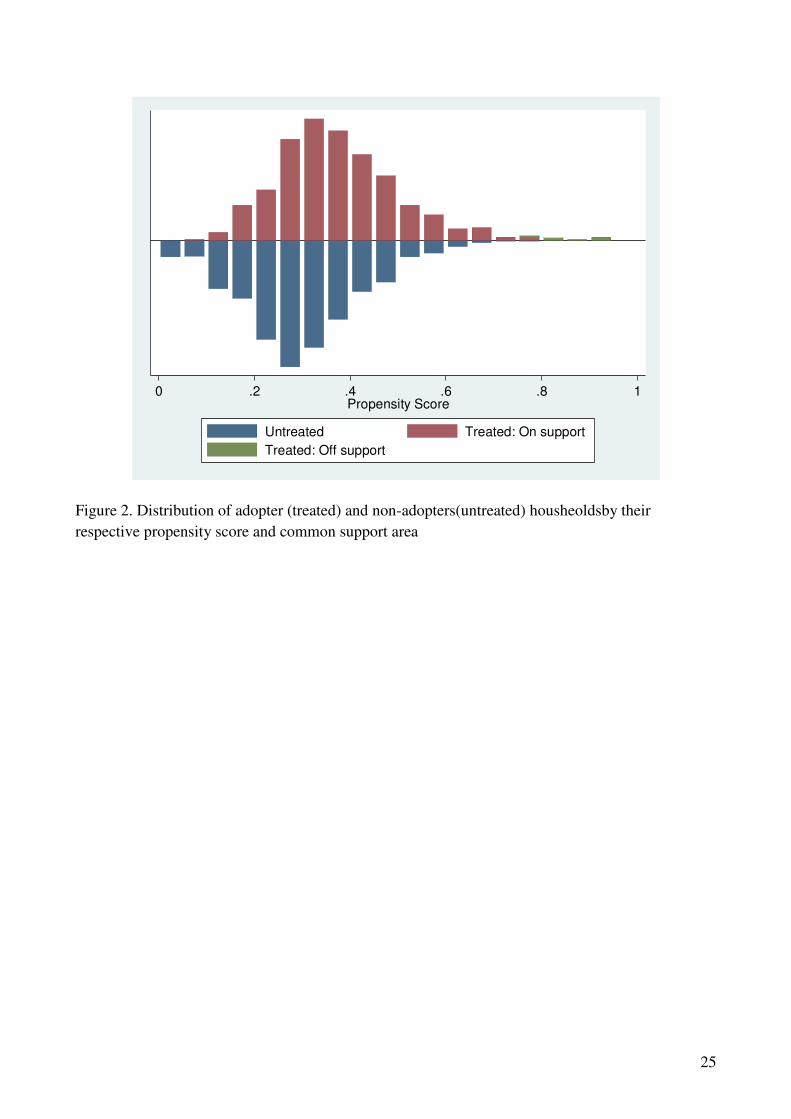
Figure 2 gives distribution of adopters and non-adopter households by their respective propensity

scores and common support area. About 98% of the sample households fall in common support

area showing that there is good overlap of adopters and non-adopters’ distribution. These data

therefore lend themselves to matching of adopters to their potential counterfactuals (in the non-

adopter categories).

< Figure 2 here >

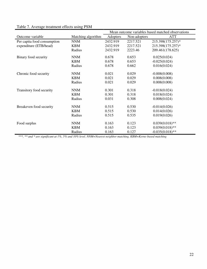
In table 7, using three matching algorithms (nearest neighbor, kernel and radius matching),

average treatment effects are presented based on propensity score matching method. For the

three matching algorithms, there is a significant difference in per-capita food consumption

between adopters and non-adopter households. In addition, the self-reported food security status

of households is significantly different between adopters and non-adopters particularly for those

who reported their status as food surplus.

< Table 7 here >

12

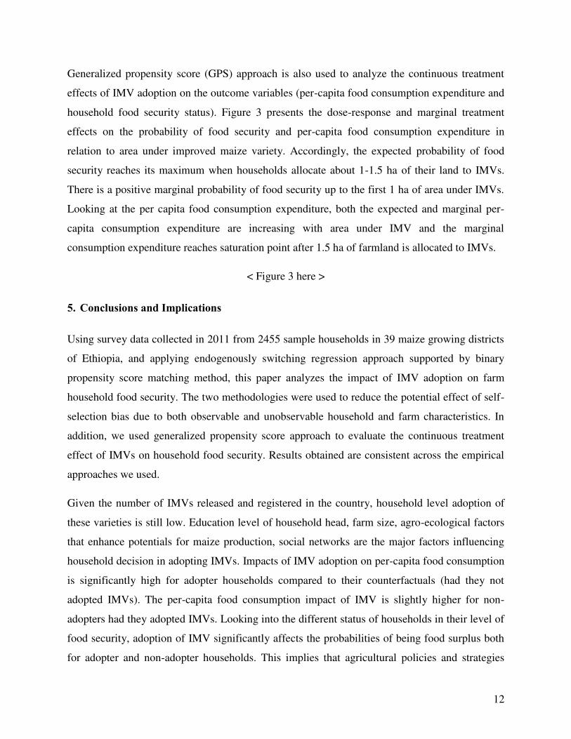
Generalized propensity score (GPS) approach is also used to analyze the continuous treatment

effects of IMV adoption on the outcome variables (per-capita food consumption expenditure and

household food security status). Figure 3 presents the dose-response and marginal treatment

effects on the probability of food security and per-capita food consumption expenditure in

relation to area under improved maize variety. Accordingly, the expected probability of food

security reaches its maximum when households allocate about 1-1.5 ha of their land to IMVs.

There is a positive marginal probability of food security up to the first 1 ha of area under IMVs.

Looking at the per capita food consumption expenditure, both the expected and marginal per-

capita consumption expenditure are increasing with area under IMV and the marginal

consumption expenditure reaches saturation point after 1.5 ha of farmland is allocated to IMVs.

< Figure 3 here >

5. Conclusions and Implications

Using survey data collected in 2011 from 2455 sample households in 39 maize growing districts

of Ethiopia, and applying endogenously switching regression approach supported by binary

propensity score matching method, this paper analyzes the impact of IMV adoption on farm

household food security. The two methodologies were used to reduce the potential effect of self-

selection bias due to both observable and unobservable household and farm characteristics. In

addition, we used generalized propensity score approach to evaluate the continuous treatment

effect of IMVs on household food security. Results obtained are consistent across the empirical

approaches we used.

Given the number of IMVs released and registered in the country, household level adoption of

these varieties is still low. Education level of household head, farm size, agro-ecological factors

that enhance potentials for maize production, social networks are the major factors influencing

household decision in adopting IMVs. Impacts of IMV adoption on per-capita food consumption

is significantly high for adopter households compared to their counterfactuals (had they not

adopted IMVs). The per-capita food consumption impact of IMV is slightly higher for non-

adopters had they adopted IMVs. Looking into the different status of households in their level of

food security, adoption of IMV significantly affects the probabilities of being food surplus both

for adopter and non-adopter households. This implies that agricultural policies and strategies

13

targeting farm household food security in maize-based systems shall encourage the adoption of

IMVs.

Acknowledgements

The authors would like to acknowledge The Standing Panel for Impact Analysis (SPIA) in the

CGIAR for financing the Diffusion and Impact of Improved Varieties in Africa (DIIVA) project.

Data used in the analysis were collected through the financial support from DIIVA project. In

addition, part of the survey was covered under the Sustainable Intensification in Maize-Legume

Cropping Systems for Food Security in Eastern and Southern Africa (SIMLESA) program

funded by the Australian Government through the Australian Center for International

Agricultural Research (ACIAR).

References

Abdulai, A., Huffman, W., 2014. The adoption and impact of soil and water conservation

technology: An endogenous switching regression application. Land Econ. 90(1), 26-43.

Alene, D.A., Manyong, V.M., 2007. The effects of education on agricultural productivity under

traditional and improved technology in northern Nigeria: An endogenous switching regression

analysis. Empir. Econ. 32,141-159.

Amare, M., Asfaw, S., Shiferaw, B., 2012. Welfare impacts of maize-pigeonpea intensification

in Tanzania. Agric. Econ. 43(1), 27-43.

Asfaw, S., Shiferaw, B., Simtowe, F., Lipper, L., 2012. Impact of modern agricultural

technologies on smallholder welfare: Evidence from Tanzania and Ethiopia. Food Policy. 37(3),

283-295.

Beddington, J., 2010. Food Security: Contributions from Science to a new and greener

revolution. Philos T Roy Soc B. 365:61-71.

Bia, M., Mattei, A., 2007. Application of the Generalized Poropensity Score. Evaluation of

public contributions to Piedmont enterprises. Working Paper n. 89. Department of Public Policy

and Public Choice (POLIS) Universita del Piemonte Orientale ‘Amedeo Avogadro’ Alessandria.

14

Brown, M.E., Funk, C.C., 2008. Food Security under Climate Change. Science. 319:580-581.

Carter, D.W., Milon. J.W., 2005. Price Knowledge in Household Demand for Utility Services.

Land Econ. 81, 265-283.

CSA, 2014a. Report on Area and production of major crops (Volume I). The Federal Democratic

Republic of Ethiopia. Central Statistical Agency, May 2014, Addis Ababa.

CSA, 2014b. Report on Crop and livestock product Utilization (Volume VII). The Federal

Democratic Republic of Ethiopia. Central Statistical Agency, September 2014, Addis Ababa.

Di Falco, S., Veronesi, M., Yusuf, M., 2011. Does adaptation to climate change provide food

security? A micro-perspective from Ethiopia. Am. J. Agr.Econ. 93(3), 829-846.

FAO, 2015. The state of food security in the World. Food and Agriculture Organization of the

United Nations, Rome.

Feleke, S., Zegeye, T., 2006. Adoption of improved maize varieties in Southern Ethiopia: Factors

and strategy options. Food Policy. 31(5), 442–457.

Godfray,H.C.J., Beddington, J.R., Crute, I.R., Haddad, L., Lawrence, D., Muir, J.F., Pretty, J.,

Robinson, S., Thomas, S.M., Toulmin, C. 2010. Food Security: The Challenge of feeding 9

Billion People. Science. 327:812-818.

Hirano, K., Imbens, G.W., 2004. The Propensity Score with Continuous Treatments.

http://scholar.harvard.edu/imbens/files/hir_07feb04.pdf

Kassa, Y., Kakrippai, R.S., Legesse, B., 2013. Determinants of adoption of improved maize

varieties for male headed and female headed households in West Harerghe zone, Ethiopia. Int. J.

Econ. Behav. Organ. 1(4), 33-38

Kassie, M., Jaleta, M., Mattei A., 2014. Evaluating the impact of improved maize varieties on

food security in Rural Tanzania: Evidence from a continuous treatment approach. Food Security.

6(2), 217-230.

MoA, 2012. Crop Diversity Register. Issue No. 15. Ministry of Agriculture, Animal and Plant

Health Regulatory Directorate. June 2012, Addis Ababa.

15

Parry, M., Rosenzweig, C., Iglesias, A., Fischer, G., Livermore, M. 1999. Climate Change and

World food security: a new assessment. Global Environ Change. S51-S67.

Shiferaw, B., Kassie, M., Jaleta, M., Yirga, C., 2014. Adoption and Impacts of improved wheat

varieties on food security in Ethiopia. Food Policy. 44, 272-284.

Tura, M., Aredo, D., Tsegaye, W., La Rovere, R., Mwangi, W., Mwabu, G., 2010. Adoption and

continued use of improved maize seeds: Case study of central Ethiopia. Afr. J. Agr. Res. 5(17),

2350-2358.

16

Tables

Table 1. Distribution of Sample households

Maize potential

Admin Region Low Medium High Total

Tigray 55 0 0 55

Amhara 102 184 46 332

Oromia 150 863 347 1,360

Benishangul Gumuz 0 0 96 96

SNNP 0 386 98 484

Total 307 1,433 587 2,327

17

Table 2. Expected conditional and average treatment effects

Category

Decision stage

Adoption Effect To adopt

IMVs

Not to adopt

IMNs

Adopters of IMV (a) �[ �| �, � = ] (c) �[ �| �, � = ] ATT

Non-adopters of IMV (d) �[ �| �, � = ] (b) �[ �| �, � = ] ATU

Heterogeneity effect BH1 BH2 TH

Note: (a) and (b) represent observed outcomes (per-capita food consumption and household food security status);

(c) and (d) represent counterfactual outcomes (per-capita food consumption and household food security status);

Ai=1 if household i adopted IMVs;

Ai=0 if household i did not adopt IMVs;

Y1i= Per-capita food consumption and household food security status if a household adopted IMVs;

Y2i= Per-capita food consumption and household food security status if a household did not adopt IMVs;

ATT =average treatment effect on treated;

ATU=average treatment effect on untreated;

BH1=the effect of base heterogeneity for IMV adoption;

BH2=the effect of base heterogeneity for non-adoption of IMVs;

TH=transitional heterogeneity (ATT-ATU)

18

Table 3. Descriptive statistics of outcome and treatment variables

Total sample

(N=2327)

Adopters (N=632)

Non-adopters (N=1695)

Variable Description Mean Std. Dev.

Mean Std. Dev.

Mean Std. Dev.

Food consumption expenditure Per capita food consumption expenditure (Birr) 2170.680 3050.489

2388.985** 3107.870

2089.412 3025.756

Food security

Dummy_ Household food security (1=yes)_HH self-

assessment 0.666 0.472

0.685 0.465

0.659 0.474

Chronic food insecurity Dummy_ Household in chronic food insecurity (1=yes) 0.026 0.160

0.019 0.137

0.029* 0.168

Transitory food insecurity Dummy_ Household in transitory food insecurity (1=yes) 0.308 0.462

0.296 0.457

0.312 0.463

Breakeven food security Dummy_ Household in breakeven food security (1=yes) 0.530 0.499

0.522 0.500

0.533 0.499

Food surplus Dummy_ Household in food surplus food security (1=yes) 0.136 0.343

0.162** 0.369

0.126 0.332

Binary adoption Adopted improved maize varieties (1=yes) 0.272 0.445

1.000 0.000

0.000 0.000

***, ** and * are significantly higher than the other group mean at 1%, 5% and 10% level.

19

Table 4. Descriptive statistics of explanatory variables

Total sample (N=2327)

Adopters (N=632)

Non-adopters (N=1695)

Variable Description Mean Std. Dev.

Mean Std. Dev.

Mean Std. Dev.

Sex of household head Sex of household head (1=male, 0=female) 0.920 0.272

0.933* 0.249

0.914 0.280

Age of household head Age of household head (years) 42.320 12.744

41.344 13.189

42.683** 12.559

Education of household head Education of household head (years of schooling ) 2.954 3.305

3.468*** 3.469

2.762 3.222

Total farmland Total land operated by a household (ha) 2.536 2.422

2.570 2.403

2.523 2.430

Family size Household size 6.587 2.536

6.970*** 2.652

6.445 2.478

High potential Dummy_ High maize potential district (1=yes) 0.252 0.434

0.274* 0.446

0.244 0.430

Livestock owned Livestock owned (TLU) 5.415 5.366 5.782** 0.226 5.276 0.128

Medium potential Dummy_ Medium maize potential district (1=yes) 0.616 0.487

0.660*** 0.474

0.599 0.490

Low potential Dummy_ Low maize potential district(1=yes) 0.132 0.338

0.066 0.249

0.156*** 0.363

Amhara Dummy_ Amhara (1=yes) 0.143 0.350

0.184*** 0.387

0.127 0.334

Oromia Dummy_ Oromia (1=yes) 0.584 0.493

0.530 0.499

0.605*** 0.489

Benishangul Gumuz Dummy_ Benishangul Gumuz (1=yes) 0.041 0.199

0.025 0.157

0.047*** 0.212

Southern Nations and Nationalities and People Dummy_ SNNP (1=yes) 0.208 0.406

0.261*** 0.440

0.188 0.391

Tigray Dummy_ Tigray (1=yes) 0.024 0.152

0.000 0.000

0.032*** 0.177

Number of relatives Number of relatives within and outside village a household relies on 23.757 38.344

29.810*** 58.637

21.500 26.820

Number of traders Number of traders within and outside village a household knows 1.807 4.136

2.122** 2.803

1.685 4.542

Distance to main market Walking distance to main market (minutes) 89.922 69.212

98.584*** 72.620

86.693 67.636

Distance to seed dealers Walking distance to maize seed source (minutes) 56.542 67.100

56.839 59.569

56.429 69.784

Share of fertile land Share of fertile land a household owns 0.425 0.415

0.369 0.416

0.446*** 0.412

Information from government Variety information from government (1=yes) 0.733 0.442

0.726 0.446

0.736 0.441

Information from neighboring farmers Variety information from neighboring farmers (1=yes) 0.055 0.228

0.051 0.219

0.057 0.232

Need and got credit for seed Need and got credit for seed purchase (1=yes) 0.052 0.222

0.075*** 0.263

0.042 0.200

Need and got credit for fertilizer Need and got credit for fertilizer purchase (1=yes) 0.089 0.285

0.116*** 0.320

0.078 0.267

***, ** and * are significantly higher than the other group mean at 1%, 5% and 10% level.

20

Table 5. Decision of adopting IMV: Probit model

Explanatory variables Coefficient Std. Err. Marginal Effects

Sex of household head 0.039 0.125 0.014

Age of household head -0.003 0.003 -0.001

Education of household head 0.042*** 0.011 0.015

Total farmland 0.008 0.024 0.003

Family size 0.041*** 0.014 0.014

Livestock owned -0.003 0.007 -0.001

High potential 0.687*** 0.130 0.256

Medium potential 0.653*** 0.116 0.219

Amhara a 0.496*** 0.110 0.189

Oromia a 0.074 0.084 0.026

Benishangul Gumuz a -0.323* 0.193 -0.105

Number of relatives 0.004*** 0.001 0.001

Number of traders 0.014* 0.008 0.005

Distance to main market 0.001*** 0.000 0.001

Distance to seed dealers -0.001 0.001 0.001

Share of fertile land -0.154* 0.079 0.055

Variety information from government -0.042 0.082 0.015

Variety information from farmers -0.006 0.152 0.002

Maize disease constraint (1=yes) 0.104 0.069 0.037

Need and got credit for seed 0.265 0.181 0.098

Need and got credit for fertilizer 0.187 0.140 0.069

Constant -1.640*** 0.240

Number of observations -1032.54 LR chi2(20) 1752 Prob > chi2 140.95 Pseudo R2 0.000 Log likelihood 0.0639 ***, ** and * are significant at 1%, 5% and 10% level.

a Tigray region is areference

21

Table 6. Average treatment effects using endogenous switching regression model

Outcome variable Farm household type and

treatment effect

Decision stage Average treatment effect To adopt Not to adopt

Per capita food consumption Adopters (ATT) 2430.209 2122.187 308.023(55.447)*** Non-adopters (ATU) 2545.422 2233.138 312.285(37.938)***

Binary food security ATT 0.685 0.662 0.024(0.011)** ATU 0.678 0.657 0.021(0.008)***

Chronic food security ATT 0.031 0.027 0.004 (0.003) ATU 0.031 0.029 0.001(0.001)

Transitory food security ATT 0.293 0.311 -0.019(0.010)** ATU 0.299 0.313 -0.013(0.008)**

Breakeven foof security ATT 0.521 0.528 -0.007(0.008) ATU 0.518 0.533 -0.015(0.006)***

Food surplus ATT 0.162 0.134 0.027(0.008)*** ATU 0.151 0.125 0.025(0.005)***

***, ** and * are significant at 1%, 5% and 10% level. ATT=Average treatement effect on treated; ATU=Average treatment effect on

untreated

22

Table 7. Average treatment effects using PSM

Outcome variable Matching algorithm

Mean outcome variables based matched observations

Adopters Non-adopters ATT

Per capita food consumption expenditure (ETB/head)

NNM 2432.919 2217.521 215.398(175.257)* KBM 2432.919 2217.521 215.398(175.257)* Radius 2432.919 2223.46 209.461(178.625)

Binary food security NNM 0.678 0.653 0.025(0.024) KBM 0.678 0.653 -0.025(0.024) Radius 0.678 0.662 0.016(0.024)

Chronic food security NNM 0.021 0.029 -0.008(0.008) KBM 0.021 0.029 0.008(0.008) Radius 0.021 0.029 0.008(0.008)

Transitory food security NNM 0.301 0.318 -0.018(0.024) KBM 0.301 0.318 0.018(0.024) Radius 0.031 0.308 0.008(0.024)

Breakeven food security NNM 0.515 0.530 -0.014(0.026) KBM 0.515 0.530 0.014(0.026) Radius 0.515 0.535 0.019(0.026)

Food surplus NNM 0.163 0.123 0.039(0.018)** KBM 0.163 0.123 0.039(0.018)** Radius 0.163 0.127 -0.035(0.018)**

***, ** and * are significant at 1%, 5% and 10% level. NNM=Nearest neighbor matching, KBM=Kerne-based matching

23

Table A1. ESR estimates for food consumption expenditure and probabilityy of food security

Explanatory variables

Per capita food consumption (Birr)

Probability of food security

Adopters

Non-adopters

Adopters

Non-adopters

Coef. Std. Err.

Coef. Std. Err.

Coef. Std. Err.

Coef. Std. Err.

Sex of household head -796.215 910.631

-312.832 636.947

0.246 0.254

0.167 0.141

Age of household head 9.777 12.372

9.503 12.904

-0.009* 0.006

-0.002 0.003

Education of household head 62.993 61.654

14.063 35.493

-0.093*** 0.029

-0.004 0.021

Total farmland 75.747 55.070

195.930*** 35.125

0.043 0.044

0.147*** 0.041

Family size -247.517*** 56.016

-268.072*** 60.180

-0.056 0.035

-0.034 0.023

Livestock owned 2.292 22.535

7.416 13.116

0.029* 0.015

0.032** 0.013

High potential -392.167 392.256

-339.106 279.319

-1.413*** 0.465

-0.371 0.240

Medium potential 221.382 437.639

-207.231 226.719

-1.787*** 0.451

-0.665*** 0.214

Amhara a -1859.557 1393.196

64.601 647.731

-0.005*** 0.001

-0.002*** 0.001

Oromia a -1137.746 1259.191

360.161 486.594

-0.061 0.320

0.668 0.559

Benishangul Gumuz a 0.000

-341.804 563.611

0.428*** 0.153

0.791* 0.460

SNNPR a -843.939 1367.786

1798.670*** 633.037

1.955*** 0.537

1.443*** 0.456

Distance to main market -0.320 1.704

1.698 1.825

0.000 (omitted)

0.712 0.468

Share of fertile land -219.510 334.695

-182.228 258.029

0.155 0.152

0.226** 0.099

Variety information from government 452.975* 236.876

-520.339 348.425

-0.540 0.290

-0.145 0.176

Variety information from farmers -566.409** 285.454

-933.749** 457.446

-1.132*** 0.360

-0.324 0.259

Maize disease constraint (1=yes) 804.392** 382.658

190.699 222.966

0.194 0.339

0.132 0.217

Need and got credit for seed -762.090** 378.229

227.578 561.930

0.497*** 0.174

0.368*** 0.112

Need and got credit for fertilizer 253.801 376.898

-161.719 334.815

-0.541*** 0.152

-0.176* 0.093

IMR 26.466 1000.016

524.036 878.081

-2.717*** 0.727

-1.021 0.680

Constant 4641.866 2443.585

3452.706*** 1029.249

5.805*** 1.479

-0.714 0.475

Number of obs. 571

1190

568

1183

F-Value/Wald Chi2 4.32

7.72

110.66

117.16

Prob > F 0.000

0.000

0.000

0.000

R-squared/Pseudo r2 0.0835

0.0605

0.1706

0.1103

Root MSE/P 3112.8

3469.3

Log pseudo likelihood

-293.575

-675.776

***, ** and * are significant at 1%, 5% and 10% level. a Tigray region is areference.

24

Figures

Figure 1. Distribution of sample districts where the survey was conducted.

25

Figure 2. Distribution of adopter (treated) and non-adopters(untreated) housheoldsby their

respective propensity score and common support area

0 .2 .4 .6 .8 1Propensity Score

Untreated Treated: On support

Treated: Off support

26

Figure 3. Dose response and marginal treatment effects on the probability of food security and per-

capita food consumption expenditure.

20

00

25

00

30

00

35

00

40

00

0 .5 1 1.5 2 2.5

Area under improved maize variety (ha)

Dose Response Low bound

Upper bound

.5.6

.7.8

.9

0 .5 1 1.5 2 2.5Area under improved maize varieties (ha)

Dose Response Low bound

Upper bound

-50

0

0

50

01

00

01

50

0

0 .5 1 1.5 2 2.5

Area under improved maize variety (ha)

Treatment Effect Low bound

Upper bound

-.2

-.1

0.1

.2

0 .5 1 1.5 2 2.5Area under improved maize varieties (ha)

Treatment Effect Low bound

Upper bound