Embed Size (px)
Citation preview

International parity relationships between
Germany and US: a multivariate time seriesanalysis for the post Bretton-Woods period¤
Franco BevilacquaLEM - Laboratory of Economics and Management
MERIT - Maastricht Economic Research Institute on Innovation and Technology
Cinzia DaraioLEM - Laboratory of Economics and Management
June 30, 2001
Abstract
This paper investigates the e¤ects of replacing the consumer priceindex (CPI) with the wholesale price index (WPI) in the cointegrating in-ternational parity relationships found by Juselius and MacDonald (2000).
Our empirical analysis outstandingly produced results similar to theones obtained by Juselius and MacDonald, suggesting that the cointegra-tion relationships in the international parity conditions hold both for CPIand WPI.
JEL Classi…cations E31, E43, F31, F32Keywords: VAR model, cointegration, purchasing power parity, un-
covered interest rate parity.
1 IntroductionRecently, basic issues in international monetary economics concerning the va-lidity of parity conditions are receiving a growing interest also in econometrics.
Seemingly simple questions about the determinants of exchange rates be-tween countries such as Europe and US, do not still …nd adequate responses
¤This paper has been written for the Econometric Course on “The Cointegrated VARModel: Econometric Methodology and Macroeconomic Applications” by Prof. KatarinaJuselius, A.Y. 2000-2001. Doctoral Program in Economics and Management, Sant’AnnaSchool of Advanced studies, Pisa.
1
rigorously grounded on empirical data. Is the exchange rate determined by thelevel of prices as the Purchasing Power Parity (ppp) suggests? Is the exchangerate determined by the spread between the interest rates in the two countriesas the Uncovered Interest rate Parity (uip) claims? How prices react to changesin exchange rates and interest rates?
Answering to these issues becomes problematic when economic theory as-sumes that ppp and uip are stationary relations while they are empirically non-stationary both in the short and medium-long run such as a span of 20-25 years(Rogo¤ (1996). Rogo¤ refers to this problem as ”The Puchasing Power ParityPuzzle” and talks about ”the embarrassment of not being able to reject the ran-dom walk model” for the ppp while other authors doubt about the usefulness ofppp and uip1 .
This paper is aimed to show that the ppp and uip relations are indeed ex-tremely interesting when they are jointly modelled and we should not be em-barrassed when we deal with ”random walk” parity conditions. Indeed, justbecause ppp and uip behave in a nonstationary way, we may investigate thecointegration relations between the two parities i.e. the stationary long run re-lations between pseudo random walks (the ppp and the uip) that share commontrends.
This paper is based on a recent paper by Juselius and MacDonald (2000)and two ”Journal of Econometrics” articles by Juselius (1995) and Johansen andJuselius (1992). The basic feature in all these articles is that the joint modellingof international parity conditions, namely ppp and uip, produces stationaryrelations showing an important interaction between the goods (via the ppp) andthe capital markets (via the uip)2 .
Since ”there is no ”right” ppp measure” (Rogo¤ 1996)3 , we replaced theconsumer price index (CPI) considered by Juselius and MacDonald with thewholesale price index (WPI) to check whether the international parity relation-ships still cointegrate. To our surprise we outstandingly produced similar resultsto those by Juselius and MacDonald, suggesting that the cointegration relation-ships in the international parity conditions hold also if we use di¤erent measuresof prices and ppp. What is striking in our results is that even if there is no directcointegration relation between CPI and WPI both in Germany and the US, thecointegration relation found between ppp and uip still holds notwithstanding ofhow ppp is measured.
The paper is organised as follows. In section 2 we de…ne the internationalparity conditions. In section 3 we discuss the choice of the variables, the data setand we provide some preliminary visual analysis of the variables and the parityconditions. In section 4 we explain the statistical model we use to test the
1 See Colombo and Lossani (2000).2 See Juselius 1995.3 Rogo¤ (1996) put forward the idea to use even the McDonald’s ”Big Mac” index to
produce a PPP measure with the data provided by The Economist. We found this idea veryentertaining, but unfortunately the actual dataset would not allow us to use VAR (that needslong time series) and cointegration techniques in a reliable way. The Big Mac index data setby The Economist contains only the data of the last 10 years on a semester basis so that VARmodelling and cointegration are precluded.
2

parities. In section 5 we test parity conditions using a model with a minimalnumber of variables, which exclude the short interest rates. In section 6 weextend the model including also the short term interest rates. Using the movingaverage (MA) representation, the weakly exogenous variables and the long runimpacts of shocks are also discussed. Section 7 concludes and summarises themain results.
2 International parities conditions
2.1 The absolute ppp
The absolute ppp, is de…ned as:
pt ¡ p¤t ¡ st = 0 (1)
where pt is the log of the domestic price level (in our case the Germanwholesale price level index), p¤
t is the log of the foreign price level (in our casethe wholesale price level index in the US), st denotes the log of the spot exchangerate (home currency price of a unit of foreign currency). The ppp states that,once converted to a common currency, the price levels in the two countriesshould be equal.
If the ppp holds empirically, we would expect that:
pt ¡ p¤t ¡ st s I(0)
where I(0) stands for zero order integrated process.The empirical analysis con…rms two main aspects:- The ppp is a relation valid only in the very long run (temporal horizon
of more than 50 years). On a shorter temporal horizon we observe persistentdeviation from ppp (Rogo¤ 1996).
The nature of the empirical support for ppp is very dependent on the sampleperiod. If a relatively long span of data is used such as a century, there ismounting evidence that ppp is valid, although the adjustment speed of ppp istoo slow to be consistent with a traditional version of ppp (Rogo¤ 1996) andfor the recent ‡oating experience there is little evidence that ppp behaves like aI(0) process.
Juselius and MacDonald suggest that there are a number of possible reasonswhy the ppp has a so little empirical support in the short and medium run.One reason could lie in the rather weak correspondence between the measuredprices series used by researchers - usually the CPI - and the true theoreticalprices; other variables not mentioned by theory, such as institutional factors,might also be relevant. Another reason, which is a objection to traditional pppis that there may be important real determinants (such as productivity shocks,di¤erences in technology and preferences), which are responsible for introducinga stochastic trend into real exchange rates.
3
2.2 The uip
The condition of uip, is de…ned as:
Et¢lst+l ¡ ilt + il¤t = 0 (2)
where ilt denotes a long term bond yield with maturity t + l, Et denotesthe conditional expectations operator on the basis of time-t information set.The uip states that, in the capital market, the interest rate di¤erential betweenthe two countries is equal to the expected change in the spot exchange rates(Juselius 1995). Hence, once converted to a common currency, the interestrates in the two countries should be equal. If this were not, investors wouldhave the incentive to move capitals from the country where the interest rate islower to the country where the interest rate is higher till equilibrium. Thus, theuip is an arbitrage relation that describes an equilibrium in the capital markets(Colombo and Lossani 2000).
If the uip hold empirically, we would expect that:
Et¢lst+l ¡ ilt + il¤t s I(0)
Juselius (1995) and Juselius and MacDonald (2000) maintain that empiricaltests by other authors (Cumby and Obstfeld 1981) have con…rmed that the uip,like the ppp, is a non stationary relation.
2.3 Combining the ppp with the uip
In this paper we also will add evidence that ppp and uip as such do not …ndempirical support, however, as Juselius and MacDonald (2000), our aim is tocheck whether a linear combination of the two parities are able to generate astationary relation.
Before we arrive to a …nal equation to test that includes both parities, fromthe uip equation we have:
ilt ¡ il¤t = Et¢lst+l (3)
From ppp, di¤erencing and taking the expected change of exchange rate, wehave:
Et¢lst+l = Et¢lpt+l ¡ Et¢lp¤t+l (4)
Thus:
ilt ¡ il¤t = Et¢lpt+l ¡ Et¢lp¤t+l (5)
i.e.:
ilt ¡ il¤t ¡ Et¢lpt+l + Et¢lp¤t+l = 0
4

Therefore a relation that combines the ppp and the uip may be written as:
ilt ¡ il¤t ¡ Et¢lpt+l + Et¢lp¤t+l = pt ¡ p¤
t ¡ st (6)
or alternatively:
ilt ¡ il¤t = Et(¢lpt+l ¡ ¢lp¤t+l) + pppt
that would …nd empirical support if:
ilt ¡ il¤t ¡ pppt ¡ Et(¢lpt+l ¡ ¢lp¤t+l) s I(0)
and this would be the case of either:
ilt ¡ il¤t s I(0), pppt s I(0) and Et(¢lpt+l ¡ ¢lp¤t+l) s I(0)
or:
ilt ¡ il¤t s I(1) , pppt s I(1) and Et(¢lpt+l ¡ ¢lp¤t+l) s I(1)
but ilt ¡ il¤t ¡ pppt ¡ Et(¢lpt+l ¡ ¢lp¤t+l) s I(0).
If we assume rational expectations in prices:
Et(¢lpt+l ¡ ¢lp¤t+l) = (¢pt ¡ ¢p¤
t ) + vt
with vt unpredictable i.i.d. shock, we have that:
ilt ¡ il¤t = (¢pt ¡ ¢p¤t ) + pppt + vt (7)
if we relax the rational expectations hypothesis, for example if we admit badguys like the chartists that do not ever conform to rational rules, we might con-sider that the following and more general equation might be more appropriate:
ilt ¡ il¤t = !1(¢pt ¡ ¢p¤t ) + !2pppt + vt (8)
with ! parameters, and testing:
(ilt ¡ il¤t ) ¡ !1(¢pt ¡ ¢p¤t ) ¡ !2pppt s I(0) (9)
is equivalent to test whether or not equation (8) …nds empirical support.The relation expressed in (9) is the fundamental relation that we test and
would be satis…ed either in the case that:
ilt ¡ il¤t s I(0), pppt s I(0) and (¢pt ¡ ¢p¤t ) s I(0)
or:
ilt ¡ il¤t s I(1) , pppt s I(1) and (¢pt ¡ ¢p¤t ) s I(1).
Before starting the tests, a rationale choice of the variables, the sampleperiod and the data set will be discussed in the next section.
5

3 Choice of the variables, data set and a visualanalysis
3.1 Choice of the variables and data set
The variables that enter in equation (8) are:- pt, the home price index- p¤
t , the foreign price index- it, the home interest rate- i
¤, the foreign interest rate
- st, the spot exchange rateOur analysis focuses only on two ”big” countries, namely Germany and the
US and is referred to the recent ‡oat period after the end of the Bretton Woodssystem (1975-1998)4.
The choice of the countries and the sample period may be justi…ed in thefollowing way:
- It is always worth not to mix di¤erent regimes. A economic relation mighthave economic meaning in one period and be nonsense for anotherone in whicha di¤erent regime prevails. Therefore it is worth to divide the sample in regimeperiods, and conduct a di¤erent analysis for the post war era and for the postBretton woods period.
- The two countries, Germany and US, are to be considered two ”big” coun-tries during the last thirty years. I.e., in the last 25-30 years, a change in oneof the two countries will probably a¤ect the other one. Conversely, if we referto the immediate post war period, we would expect that Germany follows thechanges in the US economy, i.e. we would expect to consider Germany a smallcountry and the US a big one.
Our analysis faces also other issues concerning which category of prices andinterest rates should be analyzed. Should we consider the CPI or the Big Macindex? Generally the CPI is chosen, but there is no right answer to such aquestion; we chose the WPI. Moreover, if there is no a right ppp measure, thereis no a right measure for the uip too! Shall we consider the long or the shortinterest rate? Generally the long interest rate is chosen, we will consider both.
Therefore our database database consists of the following variables:- pt, the German, or ”home” wholesale price index- p¤
t , the US, or ”foreign”, wholesale price index- ilt, the German long bond yield (10 years)- il
¤t , the US long bond yield (10 years)
- st, the spot exchange rate, USdollar/DeutcheMark- ist , the German three month Treasury bill rate- is
¤t , the US three month Treasury bill rate
This database was provided by Prof. Juselius and was extracted from theInternational Monetary Fund CD-rom 1998. Data sources such as Datastream
4 Actually the end of the Bretton Woods system, the monetary regime based on convert-ibility indirectly linked to gold, is generally dated between 1971 and 1973.
6

also contain the same and updated values. All the data are monthly, not season-ally adjusted. The starting date of our sample is July 1975, because short terminterest rate for Germany are available only from that date. We transformedprices and the exchange rate with their natural log, the yearly interest rateswere taken in percentage (i.e. divided by 100) and divided by 12 to obtain themonthly rates.
3.2 Visualizing data
The visual inspection of the data in any econometric analysis is a critical …rststep in any econometric analysis (Enders 1995). The graphs of the time seriesof all the variables relevant for the paper are shown in levels and di¤erences.
3.2.1 Prices and In‡ation rates
In this subsection we want to show that prices seem to be I(2), in‡ation ratesI(1) but (¢pt ¡ ¢p¤
t ) s I(1).Prices and its di¤erences, i.e. in‡ation rates, show a rapid increase in the
70s and a more stable pattern in the 80s and 90s both in Germany (see Fig.1, LGEWPI time series, we call LGEWPI, the log of German wholesale priceindex)5
LGEWPILEVEL
1975 1977 1979 1981 1983 1985 1987 1989 1991 1993 1995 19974.16
4.24
4.32
4.40
4.48
4.56
4.64
4.72
DIFFERENCE
1975 1977 1979 1981 1983 1985 1987 1989 1991 1993 1995 1997-0.016
-0.012
-0.008
-0.004
0.000
0.004
0.008
0.012
0.016
Fig.1: The log of WPI index in Germany.
and in the US (see Fig.2 LUSWPI time series, we call LUSWPI, the log ofthe US wholesale price index).
5 All the graphs and the cointegration analysis in this paper has been produced by CATSfor RATS software, Hansen and Juselius (1994).
7

LUSWPILEVEL
1975 1977 1979 1981 1983 1985 1987 1989 1991 1993 1995 19973.9
4.0
4.1
4.2
4.3
4.4
4.5
4.6
4.7
4.8
DIFFERENCE
1975 1977 1979 1981 1983 1985 1987 1989 1991 1993 1995 1997-0.020
-0.015
-0.010
-0.005
0.000
0.005
0.010
0.015
0.020
0.025
Fig.2: The log of WPI index in the US.
We also noticed that the wholesale price index is much more volatile thanthe consumer price index shown in the next two …gures for Germany andUS (see Fig. 3, LGECPI time series, we call LGECPI, the log of the consumerprice index in Germany; in Fig. 4 see LUSCPI where we call LUSCPI the logof the US consumer price index).
LGECPILEVEL
1975 1977 1979 1981 1983 1985 1987 1989 1991 1993 1995 19974.1
4.2
4.3
4.4
4.5
4.6
4.7
4.8
DIFFERENCE
1975 1977 1979 1981 1983 1985 1987 1989 1991 1993 1995 1997-0.005
0.000
0.005
0.010
0.015
0.020
Fig.3: The log CPI index in Germany.
8

LUSCPILEVEL
1975 1977 1979 1981 1983 1985 1987 1989 1991 1993 1995 19973.68
3.84
4.00
4.16
4.32
4.48
4.64
4.80
4.96
DIFFERENCE
1975 1977 1979 1981 1983 1985 1987 1989 1991 1993 1995 1997-0.0050
-0.0025
0.0000
0.0025
0.0050
0.0075
0.0100
0.0125
0.0150
Fig. 4: The log of CPI index in the US.
The common feature in Fig. 1-4 is that prices show a decidedly positive trendor drift throughout the whole period, while their …rst di¤erences i.e. in‡ationrates, have a positive mean. These are obvious results. But from these simplegraphs we may …nd other interesting characteristics:
- prices seem to be highly autocorrelated and in‡ation too. Moreover itseems also that both mean and variance vary over time! Both graphs, either ofprices or in‡ations, seem decidedly di¤erent from the one obtained from a whitenoise I(0) process distributed as a uniform distribution with zero mean and unitvariance (see Fig. 5).
I(0 ) , w h it e n o is e p ro c e s s
- 0 . 6
- 0 . 4
- 0 . 2
0
0 . 2
0 . 4
0 . 6
t im e
Fig 5: Graph of a white noise process.
9

From these …rst graphs we might have some idea about the type of processof both prices and in‡ation. In‡ation seem far to be a pure I(1) process as theone in Fig. 6,
I(1 ) p ro c e s s
t im e
Fig. 6: Example of a I(1) process generated by white noise.
but still is quite di¤erent from the I(0) process in Fig. 5. Is in‡ation aI(0) or a I(1) process? The time series reported in Fig. 7 showsomething interesting: the time series is arti…cial and is composed by 75% by aI(0) component (the one in Fig. 5) and by 25% by a I(1) (the one in Fig. 6), theautocorrelation seems present and both mean and variance seem to vary withtime! This is a similar pattern of in‡ation rates. Therefore we have the suspectthat in‡ation rates contain some I(1) structure hidden by noise.
- 2
- 1 .5
- 1
- 0 .5
0
0 .5
t im e
Fig. 7: Mixed process composed by 75% by a I(0) and 25% by a I(1) process.
If in‡ation rates contain a I(1) component, thus prices contain a I(2) compo-nent. Fig. 8 shows an arti…cial process generated by the summation of a I(1) (by75%) with a I(2) process (by 25%). We observe a smooth trending behaviour
10

similar6 to the one observed in prices, either CPI or WPI. Concluding, wecan state that prices might contain a I(2) component that should be taken intoaccount using a truly I(2) procedure, or alternatively in‡ation rates should beanalysed in a I(1) framework.
- 2 0 0
- 1 5 0
- 1 0 0
- 5 0
0
time
Fig. 8: Mixed process composed by 75% by a I(1) and by 25% by a I(2)process.
If we wish to compare the relation between WPI and CPI in Germany (seeFig. 9, LGEPWC time series, we call LGEPWC the spread between the log ofthe wholesales and consumer price indexes in Germany) and in the US (see Fig.10, LUSPWC time series, we call LUSPWC the spread between the log of thewholesales and consumer price indexes in the US) we observe a similar patternto Fig. 8, characterised by a smooth trending behaviour.
6 Except for the case that here the trend is negative. Mixed processes as well as pure I(2)processes might also generate growing time series or changes in trends but the peculiar featureof these processes is that the time series is rather smooth with a strong autocorrelation.
11

LGEPWCLEVEL
1975 1977 1979 1981 1983 1985 1987 1989 1991 1993 1995 1997-0.15
-0.10
-0.05
0.00
0.05
0.10
DIFFERENCE
1975 1977 1979 1981 1983 1985 1987 1989 1991 1993 1995 1997-0.015
-0.010
-0.005
0.000
0.005
0.010
0.015
Fig. 9: The spread between price indexes in Germany.
LUSPWCLEVEL
1975 1977 1979 1981 1983 1985 1987 1989 1991 1993 1995 1997-0.15
-0.10
-0.05
0.00
0.05
0.10
0.15
0.20
0.25
DIFFERENCE
1975 1977 1979 1981 1983 1985 1987 1989 1991 1993 1995 1997-0.020
-0.015
-0.010
-0.005
0.000
0.005
0.010
0.015
0.020
Fig. 10: The spread of price indexes in the US.
Moreover, if we look at the relation (pt ¡ p¤t ) (see Fig. 11, GEUSPR time
series, we call GEUSPR the spread of the log of the wholesales price indexbetween Germany and US), we observe a trending behaviour similar to Fig. 8,
12
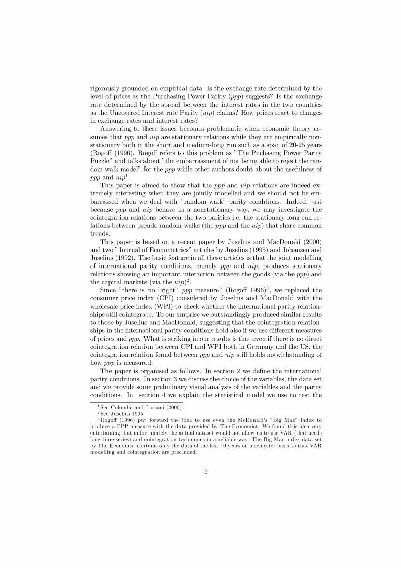
characterised by a strong autocorrelation and a rather smooth pattern, typicalof processes with components higher than I(1). We suspect that pt s I(2), p¤
t sI(2) and (pt ¡ p¤
t ) s I(2), that is, prices alone do not cointegrate. Therefore,we conclude that (¢pt ¡ ¢p¤
t ) s I(1) (see Fig. 11, lower panel).
GEUSPRLEVEL
1975 1977 1979 1981 1983 1985 1987 1989 1991 1993 1995 1997-0.10
-0.05
0.00
0.05
0.10
0.15
0.20
0.25
0.30
DIFFERENCE
1975 1977 1979 1981 1983 1985 1987 1989 1991 1993 1995 1997-0.020
-0.015
-0.010
-0.005
0.000
0.005
0.010
0.015
0.020
Fig. 11: The price spread between Germany and US.
3.2.2 Exchange rates and ppp
We have noticed that prices clearly contain structures higher than I(1). Alsoexchange rates seem contain I(2) components. Its behaviour is rather smooth,with prolonged periods of appreciation and periods of depreciation, with a trendtendency consistent with a I(2) hypothesis, even if the I(2) component is notas clear as in prices. However if we closely look at Fig. 12 (see LDMUSD timeseries, we call LDMUSD the log of exchange rate of the German Mark againstthe US Dollar) and at Fig. 11, we might notice that the exchange rate and thespread of prices in the long run follow a similar trend. The sharp rise of exchangerates occurred between 1980 and 1985 could be explained to di¤erent factors,such as the increase of US …scal de…cit together with a speculative bubble ofworld-wide dimension.
13

LDMUSDLEVEL
1975 1977 1979 1981 1983 1985 1987 1989 1991 1993 1995 19970.25
0.50
0.75
1.00
1.25
DIFFERENCE
1975 1977 1979 1981 1983 1985 1987 1989 1991 1993 1995 1997-0.12
-0.08
-0.04
0.00
0.04
0.08
0.12
0.16
Fig 12: The log of exchange rate
In the case that spread prices (that is most probably a I(2) process) sharethe same trend of exchange rate (that is probably a I(2) process too), we might…nd that they cointegrate from I(2) to I(1), i.e. they are CI(2; 1). From Fig.13 (see the PPPWGE time series, we call PPPWGE the ppp calculated withthe wholesale prices) where we do not notice a typical trending behaviour ofI(2) processes, we might think that ppp behaves like a I(1) process. As Enders(1995) pointed out referring to the ppp, the series seems to meander in a fashioncharacteristic of a random walk process, i.e. ppp is a I(1) process.
PPPWGELEVEL
1975 1977 1979 1981 1983 1985 1987 1989 1991 1993 1995 1997-0.012
-0.011
-0.010
-0.009
-0.008
-0.007
-0.006
-0.005
-0.004
-0.003
DIFFERENCE
1975 1977 1979 1981 1983 1985 1987 1989 1991 1993 1995 1997-0.00125
-0.00100
-0.00075
-0.00050
-0.00025
0.00000
0.00025
0.00050
0.00075
0.00100
Fig 13: Purchasing Power Parity.
3.2.3 The interest rates and their spread
Let us see …rst the spread of interest rates. As noticed by Juselius and Mac-Donald, the spread between long bond interest rates follow a dynamics that issomewhat similar to the one of ppp (compare Fig. 14 with Fig. 13; see the
14

BONDSP time series, we call BONDSP the spread of the long term interestrates in the two countries). From the graph the bond spread could seem a I(1)process a¤ected by some heteroskedasticity (see lower panel).
BONDSPLEVEL
1975 1977 1979 1981 1983 1985 1987 1989 1991 1993 1995 1997-0.005
-0.004
-0.003
-0.002
-0.001
0.000
0.001
0.002
DIFFERENCE
1975 1977 1979 1981 1983 1985 1987 1989 1991 1993 1995 1997-0.0012
-0.0008
-0.0004
-0.0000
0.0004
0.0008
0.0012
Fig. 14: The bond rate spread.
If we look at the Treasury Bill rates we observe a strong heteroskedasticity(see lower panel Fig. 15; we called BILLSP the time series of the spread betweenTreasury Bill rates in the two countries), and a quite irregular pattern, with nolong run trending behaviour like I(2) processes. Thus the short term interestrate spread might be a I(1) process.
BILLSPLEVEL
1975 1977 1979 1981 1983 1985 1987 1989 1991 1993 1995 1997-0.0075
-0.0050
-0.0025
0.0000
0.0025
0.0050
DIFFERENCE
1975 1977 1979 1981 1983 1985 1987 1989 1991 1993 1995 1997-0.0025
0.0000
0.0025
0.0050
Fig. 15: The Treasury Bill rate spread.
Now, if the spread of interest rates are I(1) they could be the result ofthe fact that the interest rates in the two countries are I(1) and they do notcointegrate, or they are I(2) and cointegrate.
Fig. 16 and 17 suggest that both time series are a¤ected by ARCH structuresbut they do not show the typical smooth and prolonged trending behaviour of
15

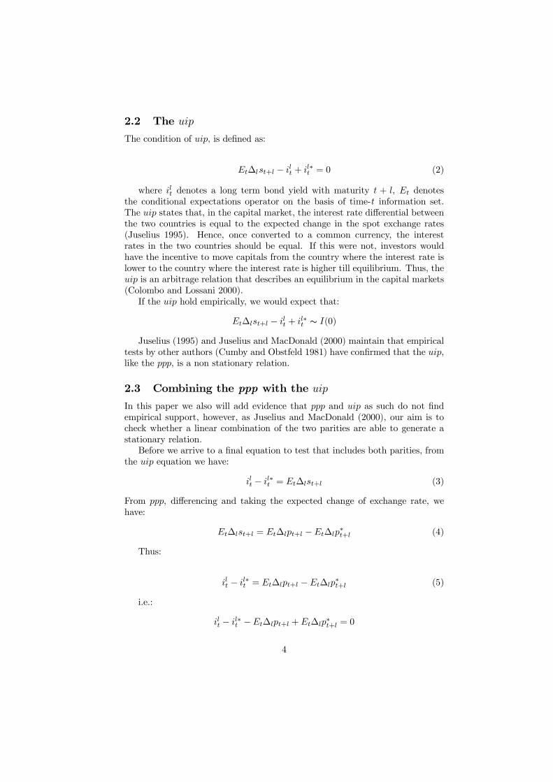
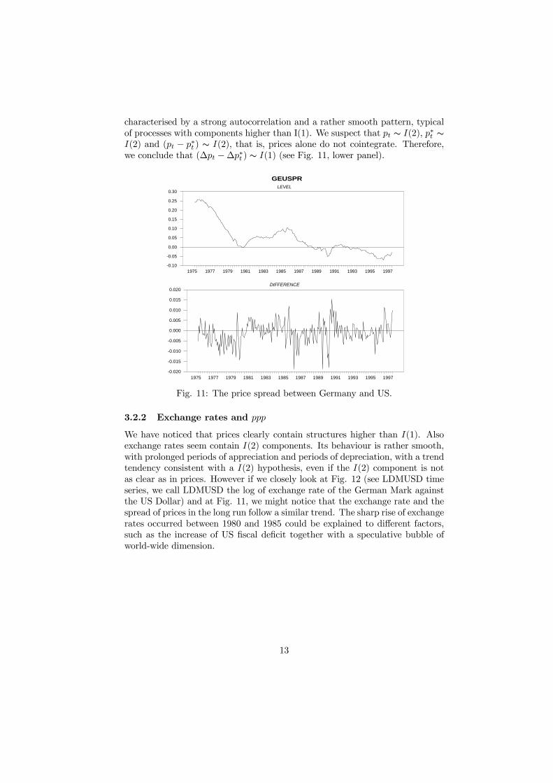
I(2) time series. Similar consideration may apply to the time series of trea-sury bill rates (Fig. 18 and 19), so we might think that interest rates are allI(1) processes with strong heteroskedasticity and they do not cointegrate bythemselves.
GEBONDLEVEL
1975 1977 1979 1981 1983 1985 1987 1989 1991 1993 1995 19970.004
0.005
0.006
0.007
0.008
0.009
0.010
DIFFERENCE
1975 1977 1979 1981 1983 1985 1987 1989 1991 1993 1995 1997-0.0006
-0.0004
-0.0002
-0.0000
0.0002
0.0004
0.0006
0.0008
Fig. 16: The long term interest rate in Germany.
USBONDLEVEL
1975 1977 1979 1981 1983 1985 1987 1989 1991 1993 1995 19970.004
0.005
0.006
0.007
0.008
0.009
0.010
0.011
0.012
0.013
DIFFERENCE
1975 1977 1979 1981 1983 1985 1987 1989 1991 1993 1995 1997-0.0015
-0.0010
-0.0005
0.0000
0.0005
0.0010
0.0015
Fig. 17: the long term interest rate in the US.
16
GETBILLLEVEL
1975 1977 1979 1981 1983 1985 1987 1989 1991 1993 1995 19970.002
0.003
0.004
0.005
0.006
0.007
0.008
0.009
0.010
0.011
DIFFERENCE
1975 1977 1979 1981 1983 1985 1987 1989 1991 1993 1995 1997-0.0015
-0.0010
-0.0005
0.0000
0.0005
0.0010
Fig. 18: the Treasury Bill rate in Germany.
USTBILLLEVEL
1975 1977 1979 1981 1983 1985 1987 1989 1991 1993 1995 19970.002
0.004
0.006
0.008
0.010
0.012
0.014
DIFFERENCE
1975 1977 1979 1981 1983 1985 1987 1989 1991 1993 1995 1997-0.0050
-0.0025
0.0000
0.0025
Fig 19: The US Treasury Bill rate.
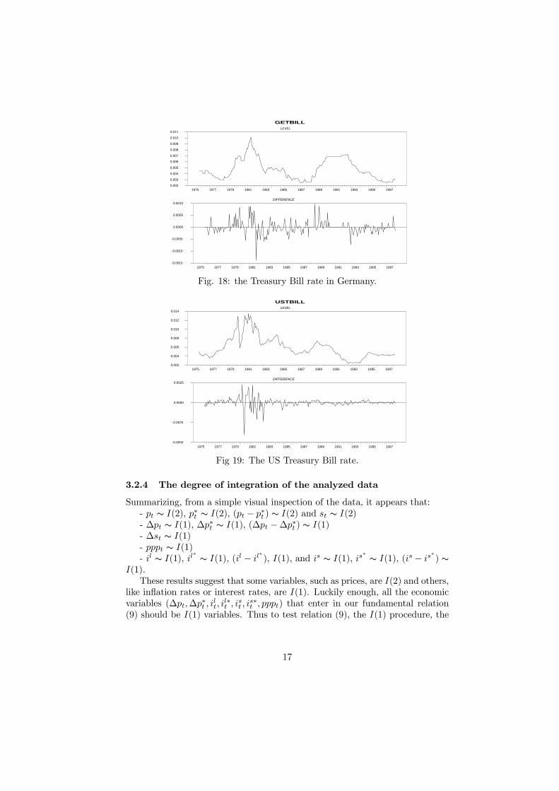
3.2.4 The degree of integration of the analyzed data
Summarizing, from a simple visual inspection of the data, it appears that:- pt s I(2), p¤
t s I(2), (pt ¡ p¤t ) s I(2) and st s I(2)
- ¢pt s I(1), ¢p¤t s I(1), (¢pt ¡ ¢p¤
t ) s I(1)- ¢st s I(1)- pppt s I(1)- il s I(1), il
¤ s I(1), (il ¡ il¤), I(1), and is s I(1), is
¤ s I(1), (is ¡ is¤) s
I(1).These results suggest that some variables, such as prices, are I(2) and others,
like in‡ation rates or interest rates, are I(1). Luckily enough, all the economicvariables (¢pt;¢p¤
t ; ilt; i
l¤t ; ist ; i
s¤t ; pppt) that enter in our fundamental relation
(9) should be I(1) variables. Thus to test relation (9), the I(1) procedure, the
17

so called ”Johansen procedure”, might be su¢cient7 .
4 The I(1) model8
The I(1) model can be formulated in two equivalent forms: the vector autore-gressive model VAR and the vector moving average representation VMA. Whilethe VAR model enables us to single out the long run relations in the data, theVMA representation is useful for the analysis of the common trends that havegenerated the data (Juselius 1995).
4.1 The VAR representation and the long run relations
The VAR model formulated in the correction error form is:
¢xt = ¡1¢xt¡1 + ::: + ¡k¡1¢xt¡k+1 + ¦xt¡1 + ¹ + ªDt + "t (10)
"t s Np (0;§), t = 1; :::; T
where p = 5 (or 7 for the extended model that includes short run interestrates) is the dimension of the VAR model, x0
t =£¢pt;¢p¤
t ; ilt; i
l¤t ; pppt
¤(or x0
t =£¢pt;¢p¤
t ; ilt; i
l¤t ; ist ; i
s¤t ; pppt
¤), x0
t s I(1), k is the lag length, Dt deterministiccomponents such as centred seasonal and intervention dummies, ¹ trends, ¡1,...,¡k¡1, ª freely varying parameters and:
¦ = ®¯0
where ® and ¯ are p£r matrices of full rank, r is the rank of the ¦ matrix, and¯0xt is stationary, i.e. the stationary relations among nonstationary variablessuch as relation (9). The rank of the ¦ matrix is fundamental since it is equalto the number of stationary relations between the levels of the variables, i.e.the number of long run steady states towards which the process starts adjustingwhen it has been pushed away from the equilibrium (Hansen and Juselius 2000).
4.2 The VMA representation
The VMA representation is used to analyse the common trends that have gen-erated the data, i.e. the pushing forces from equilibrium that create the nonstationary property in the data.
The VMA representation is the following:
7 The I(1) procedure can be applied only to the variables that are ”at most” I(1). Thismeans that not all the individual variables xt have to be I(1). They can be also I(0), but notmore than I(1). This was the reason why it was necessary to build a model with variablesthat were integrated not more than I(1).
8 See Johansen (1995), Hansen and Johansen (1998) for the mathematical statistical analysisof the I(1) model and cointegration.
18

xt = CtX
i=1
"i + CtX
i=1
ªDi + C¹t + C¤ (L) ("t + ªDt + ¹) (11)
where
C = ¯?
µ®0
?
µI ¡
k¡1P1
¡i
¶¯?
¶¡1
®0?
®? and ¯? are (p ¡ r) £ (p ¡ r) matrices orthogonal to ® and ¯, while theC matrix is of reduced rank of order (p ¡ r).
The component CtP
i=1"i is really important since it represents stochastic
trends of the process9 . But how many stochastic trends are in the process?We can guess it by means of economic considerations, but we can also measureit with the rank of the C matrix. The rank is equal to the number of stochastictrends that push economic variables away from steady states. The VMA repre-sentation is of unavailable help since it shows how common trends a¤ect all thevariables of the system (see section 5.6 and 6.4).
4.3 ”General to speci…c” and ”speci…c to general” ap-proach
We adopt a ”general to speci…c” principle in statistical modelling and a ”speci…cto general” approach in the choice of variables. By imposing restrictions onthe VAR such as reduced rank restrictions, zero parameter restrictions andother parameter restrictions, the idea is to arrive to a parsimonious model witheconomically interpretable coe¢cients (Juselius and MacDonald 2000).
In the system represented by relation (10) the vector xt is composed by …veor seven variables. It had rather better to begin to analyse small models sincefor each added variable we have (p+1)¤k new parameters in the system. If thelag length is k = 3 (as in our case), and we have a system of …ve variables and weadd two variables we have (5+1)¤3+(6+1)¤3 = 39 parameters more that needto be estimated. Of course when the sample is small (less than 100 observationsfor instance, like quarterly macroeconomic models) it is often impossible toestimate the model because the number of parameters to estimate is greaterthan the number of observations. In our case we have about 270 observationsso we might estimate directly also system with seven variables. However is notadvantageous estimate it directly. In fact, reducing at minimum the numberof variables often helps in identify the cointegration relations and the identi…edcointegration relations remain valid in a more extended model. This property is
9 While CtP
i=1ªDi + C¹t are non stationary deterministic components,
C¤ (L) ("t) and C¤ (L) (ªDt + ¹) stationary stochastic and deterministic componentsof the process xt.
19
called invariance of the cointegration relations in extended sets. If cointegrationis found within a small set of variables, the same cointegration relations are validwithin any larger set of variables. The gradual expansion of the information setfacilitates an analysis of the sensitivity of the results associated with the ”ceterisparibus” assumption. This strategy is known as ”speci…c to general” approach inthe choice of variables (see Hendry and Juselius 2000, Juselius and MacDonald2000). Thus we …rst analyse the small model (x0
t =£¢pt;¢p¤
t ; ilt; i
l¤t ; pppt
¤)
excluding short term interest rates before analysing the extended model withall the seven variables (x0
t =£¢pt;¢p¤
t ; ilt; i
l¤t ; ist ; i
s¤t ; pppt
¤).
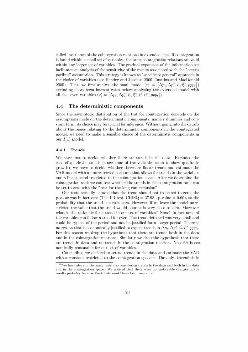
4.4 The deterministic components
Since the asymptotic distribution of the test for cointegration depends on theassumptions made on the deterministic components, namely dummies and con-stant term, its choice may be crucial for inference. Without going into the detailsabout the issues relating to the deterministic components in the cointegratedmodel, we need to make a sensible choice of the deterministic components inour I(1) model.
4.4.1 Trends
We have …rst to decide whether there are trends in the data. Excluded thecase of quadratic trends (since none of the variables seem to show quadraticgrowth), we have to decide whether there are linear trends and estimate theVAR model with an unrestricted constant that allows for trends in the variablesand a linear trend restricted to the cointegration space. After we determine thecointegration rank we can test whether the trends in the cointegration rank canbe set to zero with the ”test for the long run exclusion”.
Our tests actually showed that the trend should not to be set to zero, thep-value was in fact zero (The LR test, CHISQ = 37.98 , p-value = 0.00), so theprobability that the trend is zero is zero. However, if we leave the model unre-stricted the value that the trend would assume is very close to zero. Moreoverwhat is the rationale for a trend in our set of variables? None! In fact none ofthe variables can follow a trend for ever. The trend detected was very small andcould be typical of the period and not be justi…ed for a longer period. There isno reason that is economically justi…ed to expect trends in ¢pt;¢p¤
t ; ilt; i
l¤t ; pppt.
For this reason we drop the hypothesis that there are trends both in the dataand in the cointegration relations. Similarly we drop the hypothesis that thereare trends in data and no trends in the cointegration relation. No drift is eco-nomically reasonable for our set of variables.
Concluding, we decided to set no trends in the data and estimate the VARwith a constant restricted to the cointegration space10. The only deterministic
10 We have also run the same tests also considering trends in the data and both in the dataand in the cointegration space. We noticed that there were not noticeable changes in theresults probably because the trends would have been very small.
20

components, except the dummies allowed in our model in the data, were theintercepts in the cointegration relations.
4.4.2 Dummies
The likelihood-based inference methods on cointegration are derived upon thegaussian likelihood but the asymptotic properties of the methods depend onthe i:i:d: assumption of the errors (Johansen 1995 p. 29). Thus the fact thatthe residuals are not distributed normally is not so important. Generally ifwe reject the normality hypothesis (which is the null hypothesis of a test fornormality) we should check the skewness and the kurtosis to see whether theresiduals are well-behaved. If we would not include any dummy we would gethighly bad-behaved residuals especially for which regards skewness, and all theinference would result heavily distorted. To secure valid statistical inference weneed to take into account for shocks that fall outside the normality con…dencelevel. We set a dummy variable whenever the residual was larger than j3:5¾"j.
5 The ”small” modelWe needed the following dummy variables for the small model:
D0t = [Di8111;D8610;D9008;D9102;D9103;D9601]
where Dixx:yy is a :::; 0; 1;¡1; 0; ::: dummy measuring a transitory inter-vention shock in 19xx:yy and Dxx:yy is a :::; 0; 1; 0; ::: dummy measuring apermanent intervention shock. No shift dummy was needed and not included.We tested whether the these dummies were signi…cant, and hence necessary andwe found that all of them were signi…cant for at least one of the variables (seeTab. 1):
Tab:1 t ¡ values of dummies
DI8111 D8610 D9008 D9102 D9103 D9601¢pt ¡1:105 ¡6:047 2:625 ¡1:172 ¡0:963 ¡4:453¢p¤
t ¡0:816 ¡0:385 4:961 ¡4:467 ¡0:675 ¡0:550ilt ¡0:901 0:625 3:166 ¡2:895 1:706 ¡0:808il¤t ¡5:264 ¡0:671 0:909 ¡1:570 2:042 ¡0:009
pppt 1:493 ¡1:566 0:388 ¡0:095 ¡3:830 ¡0:921
5.1 Lag length and misspeci…cation tests
Probably the most important requirement for unbiased results is that estimatedresiduals show no serial correlation. If serial correlation is found adding onelag may be su¢cient to remove it. Changing the number of lags may require achange in the dummies.
21
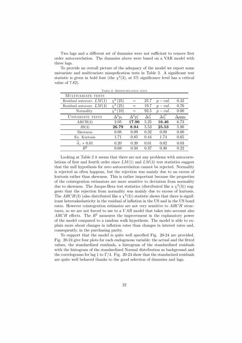
Two lags and a di¤erent set of dummies were not su¢cient to remove …rstorder autocorrelation. The dummies above were based on a VAR model withthree lags.
To provide an overall picture of the adequacy of the model we report someunivariate and multivariate misspe…cation tests in Table 2. A signi…cant teststatistic is given in bold font (the Â2(3), at 5% signi…cance level has a criticalvalue of 7:82).
Table 2: Misspecification tests
Multivariate testsResidual autocorr. LM(1) Â2 (25) = 25:7 p ¡ val: 0:42Residual autocorr. LM(4) Â2 (25) = 19:7 p ¡ val: 0:76
Normality Â2 (10) = 92:5 p ¡ val: 0:00
Univariate tests ¢2pt ¢2p¤t ¢ilt ¢il
¤t ¢pppt
ARCH(3) 2:05 17.96 5:25 16.46 6:73JB(3) 26.79 8.94 5:53 25.53 5:90
Skewness 0:08 0:09 0:32 0:09 0:00Ex. Kurtosis 1:71 0:85 0:44 1:74 0:65
^¾" £ 0:01 0:20 0:39 0:01 0:02 0:03
R2 0:69 0:50 0:37 0:30 0:22
Looking at Table 2 it seems that there are not any problems with autocorre-lations of …rst and fourth order since LM(1) and LM(4) test statistics suggestthat the null hypothesis for zero autocorrelation cannot be rejected. Normalityis rejected as often happens, but the rejection was mainly due to an excess ofkurtosis rather than skewness. This is rather important because the propertiesof the cointegration estimators are more sensitive to deviation from normalitydue to skewness. The Jarque-Bera test statistics (distributed like a Â2(3)) sug-gests that the rejection from normality was mainly due to excess of kurtosis.The ARCH(3) (also distributed like a Â2(3)) statistic shows that there is signif-icant heteroskedasticity in the residual of in‡ation in the US and in the US bondrates. However cointegration estimates are not very sensitive to ARCH struc-tures, so we are not forced to use to a V AR model that takes into account alsoARCH e¤ects. The R2 measures the improvement in the explanatory powerof the model compared to a random walk hypothesis. The model is able to ex-plain more about changes in in‡ation rates than changes in interest rates and,consequently, in the purchasing parity.
To support that the model is quite well speci…ed Fig. 20-24 are provided.Fig. 20-24 give four plots for each endogenous variable: the actual and the …ttedvalues, the standardized residuals, a histogram of the standardized residualswith the histogram of the standardized Normal distribution as background andthe correlograms for lag 1 to T=4. Fig. 20-24 show that the standarized residualsare quite well behaved thanks to the good selection of dummies and lags.
22

Actual and Fitted for DDIFWGE
1976 1979 1982 1985 1988 1991 1994 1997-0.020
-0.015
-0.010
-0.005
0.000
0.005
0.010
0.015
Standardized Residuals
1976 1979 1982 1985 1988 1991 1994 1997-4
-3
-2
-1
0
1
2
3
Histogram of Standardized Residuals
0.00
0.08
0.16
0.24
0.32
0.40
0.48
0.56Normal
DDIFWGE
Correlogram of residuals
Lag
10 20 30 40 50 60-1.00
-0.75
-0.50
-0.25
0.00
0.25
0.50
0.75
1.00
Fig. 20: estimated residuals in the German in‡ation.
Actual and Fitted for DDIFWUS
1976 1979 1982 1985 1988 1991 1994 1997-0.03
-0.02
-0.01
0.00
0.01
0.02
Standardized Residuals
1976 1979 1982 1985 1988 1991 1994 1997-3
-2
-1
0
1
2
3
Histogram of Standardized Residuals
0.0
0.1
0.2
0.3
0.4
0.5
0.6Normal
DDIFWUS
Correlogram of residuals
Lag
10 20 30 40 50 60
-1.00
-0.75
-0.50
-0.25
0.00
0.25
0.50
0.75
1.00
Fig. 21: estimated residuals in the US in‡ation.
Actual and Fitted for DGEBOND
1976 1979 1982 1985 1988 1991 1994 1997-0.00054
-0.00036
-0.00018
0.00000
0.00018
0.00036
0.00054
0.00072
Standardized Residuals
1976 1979 1982 1985 1988 1991 1994 1997-4
-3
-2
-1
0
1
2
3
Histogram of Standardized Residuals
0.00
0.08
0.16
0.24
0.32
0.40
0.48
0.56Normal
DGEBOND
Correlogram of residuals
Lag
10 20 30 40 50 60
-1.00
-0.75
-0.50
-0.25
0.00
0.25
0.50
0.75
1.00
Fig. 22: estimated residuals in the German bond rate.
23

Actual and Fitted for DUSBOND
1976 1979 1982 1985 1988 1991 1994 1997
-0.0020
-0.0015
-0.0010
-0.0005
0.0000
0.0005
0.0010
0.0015
Standardized Residuals
1976 1979 1982 1985 1988 1991 1994 1997
-4
-3
-2
-1
0
1
2
3
4
Histogram of Standardized Residuals
0.0
0.1
0.2
0.3
0.4
0.5
0.6
0.7Normal
DUSBOND
Correlogram of residuals
Lag
10 20 30 40 50 60
-1.00
-0.75
-0.50
-0.25
0.00
0.25
0.50
0.75
1.00
Fig. 23: estimated residuals in the US bond rate.
Actual and Fitted for DPPPWGE
1976 1979 1982 1985 1988 1991 1994 1997
-0.00125
-0.00100
-0.00075
-0.00050
-0.00025
0.00000
0.00025
0.00050
0.00075
0.00100
Standardized Residuals
1976 1979 1982 1985 1988 1991 1994 1997
-3.6
-2.4
-1.2
0.0
1.2
2.4
3.6
Histogram of Standardized Residuals
0.0
0.1
0.2
0.3
0.4
0.5
0.6Normal
DPPPWGE
Correlogram of residuals
Lag
10 20 30 40 50 60
-1.00
-0.75
-0.50
-0.25
0.00
0.25
0.50
0.75
1.00
Fig. 24: estimated residuals in the PPP.
5.2 Determination of the cointegration rank
The Eigenvalues of the ¦ matrix are reported in Table 3. We notice that threeeigenvalues are quite close to zero. How many of them are signi…cantly di¤erentfrom zero? This question is fundamental since the rank of the ¦ matrix is equalto p less the number of zero eigenvalues.
If we could set three eigenvalues to zero, it would mean that the rank is equalto 5-3=2, i.e. there would be two linearly independent stationary relations.
To discriminate zero eigenvalues from non-zero eigenvalues, i.e. to calculatethe cointegration rank, we can use the Trace test and the Lambda Max test.Table 3 shows that the null hypothesis of the Trace test, r = < 2 against r > 2cannot be rejected at 10% signi…cance level, while the null hypothesis of theLambda Max test r = 2 against r = 3 is rejected by little.
Because the asymptotic distributions of these statistics can be rather badapproximations to the true small sample distributions we calculate in table 4the …ve largest roots of the companion matrix of ¦ to help us in the choice ofthe cointegration rank. Either in case the model is unrestricted, or the rank of¦ is set to 2 or 3, there are 3 roots that are equal or very close to one. Since thenumber of roots of the companion matrix of ¦ is complementary to the rank ofthe ¦, since p = 5, r = 2 and p ¡ r are roots of the companion matrix set to
24
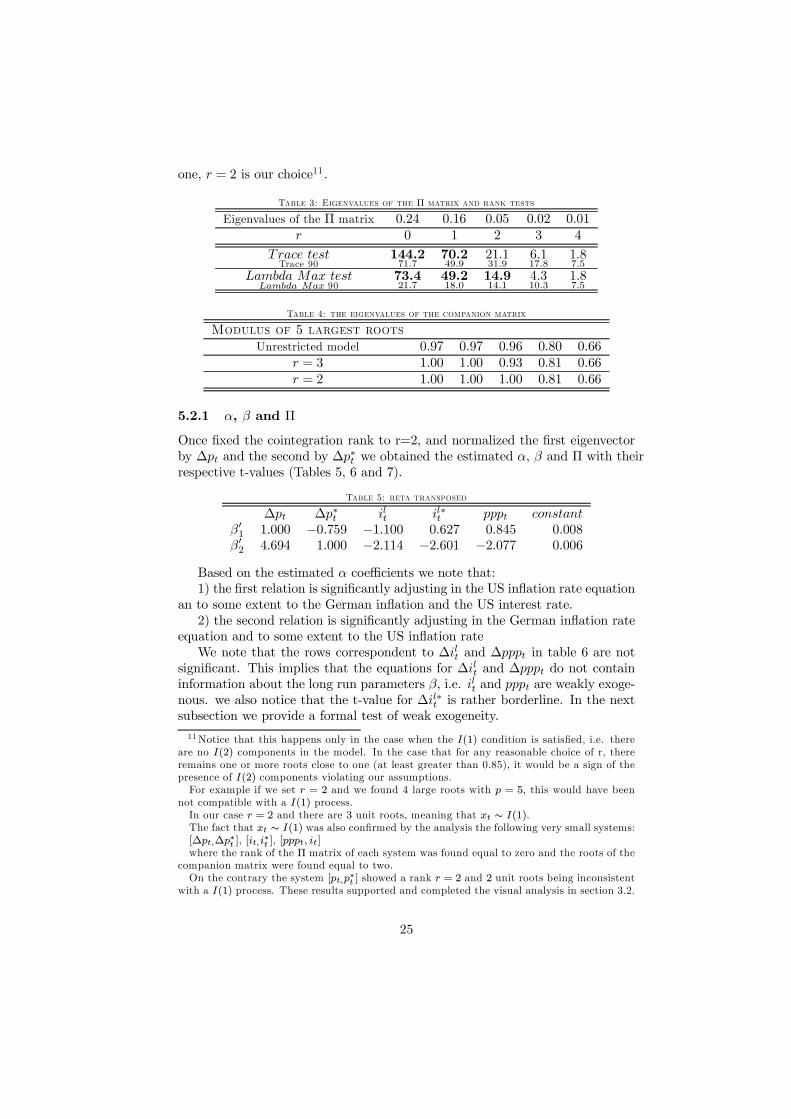
one, r = 2 is our choice11.
Table 3: Eigenvalues of the ¦ matrix and rank tests
Eigenvalues of the ¦ matrix 0:24 0:16 0:05 0:02 0:01r 0 1 2 3 4
Trace testTrace 90
144.271:7
70.249:9
21:131:9
6:117:8
1:87:5
Lambda Max testLambda Max 90
73.421:7
49.218:0
14.914:1
4:310:3
1:87:5
Table 4: the eigenvalues of the companion matrix
Modulus of 5 largest rootsUnrestricted model 0:97 0:97 0:96 0:80 0:66
r = 3 1:00 1:00 0:93 0:81 0:66r = 2 1:00 1:00 1:00 0:81 0:66
5.2.1 ®, ¯ and ¦
Once …xed the cointegration rank to r=2, and normalized the …rst eigenvectorby ¢pt and the second by ¢p¤
t we obtained the estimated ®, ¯ and ¦ with theirrespective t-values (Tables 5, 6 and 7).
Table 5: beta transposed
¢pt ¢p¤t ilt il¤t pppt constant
¯01 1:000 ¡0:759 ¡1:100 0:627 0:845 0:008
¯02 4:694 1:000 ¡2:114 ¡2:601 ¡2:077 0:006
Based on the estimated ® coe¢cients we note that:1) the …rst relation is signi…cantly adjusting in the US in‡ation rate equation
an to some extent to the German in‡ation and the US interest rate.2) the second relation is signi…cantly adjusting in the German in‡ation rate
equation and to some extent to the US in‡ation rateWe note that the rows correspondent to ¢ilt and ¢pppt in table 6 are not
signi…cant. This implies that the equations for ¢ilt and ¢pppt do not containinformation about the long run parameters ¯, i.e. ilt and pppt are weakly exoge-nous. we also notice that the t-value for ¢il¤t is rather borderline. In the nextsubsection we provide a formal test of weak exogeneity.
11 Notice that this happens only in the case when the I(1) condition is satis…ed, i.e. thereare no I(2) components in the model. In the case that for any reasonable choice of r, thereremains one or more roots close to one (at least greater than 0.85), it would be a sign of thepresence of I(2) components violating our assumptions.
For example if we set r = 2 and we found 4 large roots with p = 5, this would have beennot compatible with a I(1) process.
In our case r = 2 and there are 3 unit roots, meaning that xt s I(1).The fact that xt s I(1) was also con…rmed by the analysis the following very small systems:[¢pt;¢p¤t ], [it;i
¤t ], [pppt; it]
where the rank of the ¦ matrix of each system was found equal to zero and the roots of thecompanion matrix were found equal to two.
On the contrary the system [pt;p¤t ] showed a rank r = 2 and 2 unit roots being inconsistentwith a I(1) process. These results supported and completed the visual analysis in section 3.2.
25

Table 6: ALPHA, T-VALUES FOR ALPHA^®1
^®2
¢2pt -0.113¡2:081
-0.071¡6:192
¢2p¤t 0.714
7:036-0.062¡2:899
¢ilt 0:0051:249
0:0011:368
¢il¤t 0.0162:275
0:0021:397
¢pppt 0:0070:916
¡0:002¡1:458
In the ¦ matrix, the rows give the estimates of the combined e¤ect of the twocointegration relation. The in‡ation rates are both equilibrium error correcting,while the German interest rate and the pppt are not. Again the t-values for il¤tare borderline.
Table 7: ¦ matrix and t-values
¢pt ¢p¤t ilt il¤t pppt constant
¢2pt -0.448¡5:845
0:0140:336
0.2754:265
0.1152:532
0:0531:018
-0.001¡3:078
¢2p¤t 0.421
2:937-0.605¡7:557
-0.654¡5:420
0.6107:196
0.7347:579
0.0056:458
¢ilt 0:0000:080
0:0051:572
0:0030:641
¡0:006¡1:842
¡0:007¡1:740
¡0:000¡1:006
¢il¤t ¡0:006¡0:626
0.0142:567
0:0131:579
-0.015¡2:631
-0.018¡2:663
¡0:000¡2:012
¢pppt ¡0:018¡1:678
0:0030:489
0:0131:399
0:0020:277
¡0:001¡0:138
¡0:000¡1:145
5.3 Long run exclusion, long run weak exogeneity, sta-tionary tests12
Long run exclusion, long run weak exogeneity, stationary tests provide usefulinformation about the choice of the variables and the properties of their timeseries.
The long run exclusion test investigates whether any of the variables canbe excluded from the cointegration space, implying no relationship with theother variables. It is formulated as a zero row in ¯ and the null hypothesisis that the variable does not enter in the cointegration space. In table 8 wenotice a borderline value for the long bond interest rate in the US, but wepreferred to keep il¤t in the cointegration space also because il¤t turns out usefulfor meaningful results.
The long run weak exogeneity test investigates whether one variable in‡uencethe others without being a¤ected. It is formulated as a zero row in ® and thenull hypothesis is that the variable is weakly exogeous. If the null hypothesisis accepted, the variable pushes the system without being pushed. We noticethat ilt and pppt turned out to be weakly exogenous and il¤t assumes again aborderline value. Considering il¤t weakly exogenous is consistent with the choiceof the rank r = 2.
12 See Juselius and Hansen (2000) for details and empirical examples.
26

The last test is the test for stationarity. It investigates whether one variablecan be assumed stationary. Accepting the hypothesis implies that the variableis considered I(0). The inclusion of I(0) in a system to be analyzed with theI(1) procedure is legitimate, keeping into accout that for any stationary variablethe rank increases by one13. In our system none of the variables seem stationary.
Table 8: Tests of hypothesis about some properties of xt
¢pt ¢p¤t ilt il¤t pppt constant Â2 (º)
Long run exclusion 44.59 57.25 8.65 5.15 9.61 13.73 Â2 (2)=5.99Long run weak exogeneity 28.46 47.91 2.85 6.63 2.38 Â2 (2)=5.99
Stationarity 28.40 28.78 47.83 48.26 47.38 Â2 (4)=9.49
Lastly we tested the hypothesis that ilt, il¤
t and pppt were jointly weaklyexogenous. The p ¡ value was 0:12, suggesting that the null hypothesis couldnot be rejected. The p-value increased up to 0:28 when ilt and pppt were jointlytested. Concluding, we can consider ilt, il
¤t and pppt weakly exogenous variables,
i.e. the driving forces of the system.These results are quite similar to the ones by Juselius and MacDonald: in-
‡ation rates seem driven by interest rates and ppp and not viceversa.
5.4 Single Cointegration hypothesis
In table 8 it was shown that no variable in the vector xt is stationary by itself.Looking for cointegation relations means to search for stationary linear combi-nations of the variables xt. Single Cointegration tests test whether a restrictedrelation can be accepted leaving the other relation unrestricted. If the hypo-thetical relations exists empirically, this procedure maximizes the chance to …ndthem (Juselius and MacDonald 2000).
H1 to H4 are hypothesis on pairs of variables, such as relative in‡ation,relative interest rates, and stationary real interest rates. We notice that H3, thestationary real interest for Germany, is accepted since the p ¡ value is 0:83.
Thus:
¢pt ¡ ilt + 0:004 s I(0)
H5 and H6 are tests of variants of real interest parity in which full pro-portionality has not been imposed. Restricting the two in‡ation rates to haveunit coe¢cients and the nominal interest rates to have opposite signs (H5) isrejected. H6 that relates German interest rates with the US interest rate isaccepted with a p ¡ value is 0:65.
H7 and H8 are similar to H1 and H2 leaving ppp free to vary. Both H7 andH8 are rejected.
13 For example if we had two cointegration relation and one stationary variable, the rank ofthe ¦ matrix would be equal to three.
27

H9 and H10 are stationary real interest rates for Germany and US with pppfree to vary. Both H9 and H10 are accepted with rather high p ¡ values (0:66and 0:55).
H11 simply combines H9 and H10 and still is strongly accepted with a p ¡value equal to 0:48.
H12 describes an homogeneous relationship between German in‡ation, USin‡ation and German bond in‡ation. This relation is similar to H3. We noticethat including the US in‡ation to the German real interest rate do not makeresults more robust.
H13 is similar to H12 but it is referred to the US. Including German in‡ationto the US real interest rate we cannot accept the null hypothesis.
Testing H14 is the equivalent of testing our fundamental relation in relation(9). It is accepted with a p ¡ value equal to 0:33.
Relation (9) was (ilt¡il¤t )¡!1(¢pt¡¢p¤t )¡!2pppt. H14 is accepted meaning
that relation (9) is empirically valid with !1 = 0:985 and !2 = 1:273.Thus:
(ilt ¡ il¤t ) ¡ 0:985(¢pt ¡ ¢p¤t ) ¡ 1:273pppt ¡ 0:008 s I(0)
In the next subsection we will test jointly H14 with H3 where H3 representsthe stationary real interest rate in Germany.
We noticed that !1 and !2 are both values close to 1.We therefore tested in H15 restricting !1 to 1. H15 was accepted with a
p ¡ value equal to 0:63!We therefore tested in H16 restricting their value to 1. H16 was accepted with
a p ¡ value equal to 0:43: H16 is our preferred cointegration relation since it isperfectly economically interpretable with relation (7) where agents are assumedperfectly rational!
Thus:
(ilt ¡ il¤t ) ¡ (¢pt ¡ ¢p¤t ) ¡ pppt ¡ 0:008 s I(0)
28

Table 8: Cointegration relations
¢pt ¢p¤t ilt il¤t pppt constant Â2 (º) p ¡ val
H1 1 -1 0 0 0 0.001 13.96 0.00H2 0 0 1 -1 0 0.002 44.41 0.00H3 1 0 -1 0 0 0.004 0.86 0.83H4 0 1 0 -1 0 0.004 16.02 0.00H5 1 -1 0.217 -0.217 0 0.001 13.60 0.00H6 1 0.014 -1 -0.014 0 0.004 0.86 0.65H7 1 -1 0 0 0.639 0.005 7.02 0.03H8 0 0 -1 1 0.736 0.003 33.82 0.00H9 1 0 -1 0 0.023 0.004 0.84 0.66H10 0 1 0 -1 -1.201 -0.004 1.21 0.55H11 1 -0.439 -1 0.439 0.548 0.005 0.49 0.48H12 1 -0.084 -0.916 0 0 0.003 0.63 0.73H13 -1.989 1 0 0.989 0 -0.006 10.67 0.00H14 -0.985 0.985 1 -1 -1.273 -0.008 0.93 0.33H15 -1 1 1 -1 -1.283 -0.008 0.93 0.63H16 -1 1 1 -1 -1 -0.006 2.74 0.43
5.5 Fully speci…ed cointegrating relations
We are now ready to perform a joint test of H14 (equivalent to relation (9))with H3 (equivalent to stationary German real interest rate). The test statisticÂ2(4) was found equal to 2:07 with a p ¡ value of 0:72. The …rst vector hasbeen normalized on the German in‡ation rate and the second on the Germaninterest rate. The …rst vector is given by:
¢pt ¡ ilt + 0:004 (12)
while the second representing relation (9) is:
(ilt ¡ il¤t ) ¡ 0:985(¢pt ¡ ¢p¤t ) ¡ 1:273pppt ¡ 0:008 (13)
This is the estimated fundamental relation of our paper. It combines the pppand the uip in one relation that is strongly supported by data by a p ¡ valueof 0:72.
Notice that here !1 = 0:985 and !2 = 1:273, while in case expectations weremade fully rationally !1 = 1 and !2 = 1.
This evidence shows that agents behave quite close to the theoretical rationalcase represented by relation (7)! Therefore it was natural to jointly test H3 withH15 where !1was restricted to 1. The p ¡ value increased up to 0:84!
The …rst vector is given by:
¢pt ¡ ilt + 0:004 (14)
29

while the second vector is:
(ilt ¡ il¤t ) ¡ (¢pt ¡ ¢p¤t ) ¡ 1:278pppt ¡ 0:008 (15)
Restricting also !2 = 1, i.e. combining H3 with H16, the p¡ value was still0:69, a quite acceptable value if we consider it is perfectly consistent with theparticular assumption of perfect rationality.
The …rst vector is given by:
¢pt ¡ ilt + 0:004 (16)
while the second vector that represents relation (7) is:
(ilt ¡ il¤t ) ¡ (¢pt ¡ ¢p¤t ) ¡ pppt ¡ 0:006 (17)
In table 9, a structural representation of the cointegration space containingall the information in (16) and (17) is …nally given. The adjustment coe¢cientsare also reported. What is noticeable is that none of the adjustment parametersreferring to interest rates and ppp are signi…cant, suggesting that interest ratesand ppp are not adjusting to the two steady state relations as we would expectfrom weakly exogenous variables.
Table 9: A structural representation of the cointegration space^¯1
^¯2
^®1
^®2
¢pt 1 ¡1 ¢2pt ¡0:399¡6:0
0:0210:5
¢p¤t 0 1 ¢2p¤
t ¡0:194¡1:6
¡0:564¡7:1
ilt ¡1 1 ¢ilt 0:0081:6
0:0061:9
il¤t 0 ¡1 ¢il¤t 0:0101:2
0:0152:8
ppp1t 0 ¡1 ¢pppt ¡0:018
¡1:90:002
0:4
constant 0:004 ¡0:0061 The ppp term has been divided by 100
5.6 Common trends
We report the VMA (common trends) representation for two di¤erent cases:(i) based on the unrestricted VAR model for r = 2, (ii) based on (i) but afterhaving fully speci…ed cointegrating relations with weak exogeneity of ilt, il¤t andpppt imposed on ®.
The estimates of the C matrix in table 10 measure the total impact ofpermanent shocks to each of the variables on all other variables. A row of the Cmatrix gives an indication of which variables have been particularly importantfor the stochastic trend behaviour of the variable in the row.
30

Table 10: The estimates of the long run impact matrix C
CP ^
"¢pt
P ^"¢p¤
t
P ^"il
t
P ^"il¤
t
P ^"pppt
P ^"il
t
P ^"il¤
t
P ^"pppt
¢pt 0:0150:771
0.0172:180
1.2326:878
0.2872:943
0:0160:209
1.417:54
0.272:62
¡0:08¡0:97
¢p¤t ¡0:051
¡1:3440.0302:016
0:3981:144
0.8944:723
1.4679:669
0:421:57
1.016:84
1.028:98
ilt 0:0211:003
0:0161:947
1.3006:941
0.2372:322
¡0:103¡1:264
1.417:54
0.272:62
¡0:08¡0:97
il¤t 0:0060:235
0.0242:520
¡0:052¡0:235
1.1379:440
0:0510:532
0:020:07
1.249:70
0:080:81
pppt ¡0:038¡1:445
0:0030:287
0.5562:317
-0.329¡2:524
0.9829:391
0:41 -0.23¡2:02
0.9410:78
Based on both the unrestricted (left side of table 10) and restricted (rightside of table 10) VAR model we note that cumulative shocks to in‡ation rates inGermany have no signi…cant long run impact on any other variable. Estimatedcumulative shocks to the US in‡ation rate assume boundary t ¡ values in theunrestricted VAR model, while cumulative shocks to long term interest ratesand to ppp are highly signi…cant.
The …ndings from the restricted VMA representation suggest that (see rela-tion 18, a zero was set for not signi…cant coe¢cients):
266664
¢pt
¢p¤t
iltil
¤t
pppt
377775
=
266664
c11 c12 00 c22 c23
c11 c12 00 c42 00 c52 c53
377775
24
P"il
tP"il¤
tP"pppt
35 +
stationary anddeterministiccomponents
(18)
- In‡ation rates are adjusting.- German in‡ation rate and the long bond interest rate share the same
stochastic trend.- Shocks to the German long term interest rate speed up the German in‡ation
and to some extent changes the ppp (via exchange rates as theory suggests).- Shocks to the US long term interest rate speed up the German and US
in‡ation, pushes the German long term interest rate implying that changes inUS capital markets spread towards Europe, and has a negative e¤ect on the ppp(via exchange rates as theory suggests).
- Shocks to ppp coming from exchange rates determine positive changes toUS in‡ation.
6 The ”extended model”The ”extended model” needed many more dummies because of the many in-terventions in the Treasury Bill rates that are closely linked to the monetarypolicy. We needed the following dummy variables for the extended model:
31

D0t = [D7912;Di8003;D8005;Di8006;D8011;Di8012;D8101;D8103;D8105;D8110;D8111;Di8201;D8208;D8411;D8501;D8604;D8610;D8808;D8902;D9001;D9011;D9102;D9103;D9210;D9601].We tested whether these dummies were signi…cant, and hence necessary and
we found that all of them were highly signi…cant for at least one of the variables(not shown here).
6.1 Lag length and misspeci…cation tests
Three lags and a di¤erent set of dummies were not su¢cient to remove …rstorder autocorrelation. The dummies above were based on a VAR model withfour lags.
To provide an overall picture of the adequacy of the model we report someunivariate and multivariate misspe…cation tests in Table 11. A signi…cant teststatistic is given in bold font (the Â2(4), at 5% signi…cance level has a criticalvalue of 9:48).
Table 11: Misspeci…cation tests
Multivariate testsResidual autocorr. LM(1) Â2 (49) = 52:7 p ¡ val: = 0:33Residual autocorr. LM(4) Â2 (49) = 35:81 p ¡ val: = 0:92
Normality Â2 (14) = 144:2 p ¡ val: = 0:00
Univariate tests ¢2pt ¢2p¤t ¢ilt ¢il
¤t ¢ist ¢is
¤t ¢pppt
ARCH(4) 2:7 7:2 7:54 6:98 1:01 12:67 4:93JB(4) 14:15 0:5 3:34 12:73 8:17 46:00 11:12
Skewness 0:18 0:01 0:24 0:11 0:36 0:17 0:03Ex. Kurtosis 1:16 0:11 0:28 1:06 0:74 2:49 0:65
^¾" £ 0:01 0:18 0:34 0:01 0:02 0:01 0:02 0:03
R2 0:77 0:61 0:53 0:55 0:68 0:85 0:22
Looking at Table 11 it seems that there are not any problems with auto-correlations of …rst and fourth order since LM(1) and LM(4) test statisticssuggest that the null hypothesis for zero autocorrelation cannot be rejected.Normality is rejected, but the rejection was mainly due to an excess of kurtosisrather than skewness. The Jarque-Bera test statistics (distributed like a Â2(4))suggests that the rejection from normality was mainly due to excess of kurtosis(especially in the US short term interest rate). The ARCH(4) (also distributedlike a Â2(4)) statistic shows that there is signi…cant heteroskedasticity in the UStreasury bill rates. Comparing table 11 with table 2 in section 5, we notice thatthe large model which includes one more lag and several more dummies havebetter properties with regards to heteroskedasticity. In this case, including twonew variables, it seems that ARCH structures become less relevant.
The R2 measures the improvement in the explanatory power of the modelcompared to a random walk hypothesis. The larger model increased its expla-
32

nation power, but this could be also e¤ect of the many new dummies we haveincluded in the extended model.
To support that the model is very well speci…ed Fig. 25-31 are provided.Fig. 25-31 show that the standardised residuals are well behaved thanks to aproper choice of dummies and lags.
Actual and Fitted for DDIFWGE
1976 1979 1982 1985 1988 1991 1994 1997
-0.020
-0.015
-0.010
-0.005
0.000
0.005
0.010
0.015
Standardized Residuals
1976 1979 1982 1985 1988 1991 1994 1997
-4.0
-3.2
-2.4
-1.6
-0.8
-0.0
0.8
1.6
2.4
3.2
Histogram of Standardized Residuals
0.00
0.08
0.16
0.24
0.32
0.40
0.48
0.56
0.64Normal
DDIFWGE
Correlogram of residuals
Lag
10 20 30 40 50 60
-1.00
-0.75
-0.50
-0.25
0.00
0.25
0.50
0.75
1.00
Fig. 25: The estimated residuals of German in‡ation.
Actual and Fitted for DDIFWUS
1976 1979 1982 1985 1988 1991 1994 1997
-0.03
-0.02
-0.01
0.00
0.01
0.02
Standardized Residuals
1976 1979 1982 1985 1988 1991 1994 1997
-3
-2
-1
0
1
2
3
Histogram of Standardized Residuals
0.0
0.1
0.2
0.3
0.4
0.5
0.6Normal
DDIFWUS
Correlogram of residuals
Lag
10 20 30 40 50 60
-1.00
-0.75
-0.50
-0.25
0.00
0.25
0.50
0.75
1.00
Fig. 26: The estimated residuals of US in‡ation.
Actual and Fitted for DGEBOND
1976 1979 1982 1985 1988 1991 1994 1997
-0.0006
-0.0004
-0.0002
-0.0000
0.0002
0.0004
0.0006
0.0008
Standardized Residuals
1976 1979 1982 1985 1988 1991 1994 1997
-3.2
-2.4
-1.6
-0.8
-0.0
0.8
1.6
2.4
3.2
Histogram of Standardized Residuals
0.0
0.1
0.2
0.3
0.4
0.5
0.6
0.7Normal
DGEBOND
Correlogram of residuals
Lag
10 20 30 40 50 60
-1.00
-0.75
-0.50
-0.25
0.00
0.25
0.50
0.75
1.00
Fig. 27: The estimated residuals of the German bond rate.
33

Actual and Fitted for DUSBOND
1976 1979 1982 1985 1988 1991 1994 1997
-0.0015
-0.0010
-0.0005
0.0000
0.0005
0.0010
0.0015
Standardized Residuals
1976 1979 1982 1985 1988 1991 1994 1997
-3.6
-2.4
-1.2
0.0
1.2
2.4
3.6
Histogram of Standardized Residuals
0.0
0.1
0.2
0.3
0.4
0.5
0.6
0.7Normal
DUSBOND
Correlogram of residuals
Lag
10 20 30 40 50 60
-1.00
-0.75
-0.50
-0.25
0.00
0.25
0.50
0.75
1.00
Fig. 28: The estimated residuals of the US bond rate.
Actual and Fitted for DGETBILL
1976 1979 1982 1985 1988 1991 1994 1997
-0.0015
-0.0010
-0.0005
0.0000
0.0005
0.0010
Standardized Residuals
1976 1979 1982 1985 1988 1991 1994 1997
-3.2
-2.4
-1.6
-0.8
-0.0
0.8
1.6
2.4
3.2
Histogram of Standardized Residuals
0.0
0.1
0.2
0.3
0.4
0.5
0.6
0.7Normal
DGETBILL
Correlogram of residuals
Lag
10 20 30 40 50 60
-1.00
-0.75
-0.50
-0.25
0.00
0.25
0.50
0.75
1.00
Fig. 29: The estimated residuals of the German treasury bill rate.
Actual and Fitted for DUSTBILL
1976 1979 1982 1985 1988 1991 1994 1997
-0.0050
-0.0025
0.0000
0.0025
Standardized Residuals
1976 1979 1982 1985 1988 1991 1994 1997
-4
-3
-2
-1
0
1
2
3
4
Histogram of Standardized Residuals
0.00
0.25
0.50
0.75Normal
DUSTBILL
Correlogram of residuals
Lag
10 20 30 40 50 60
-1.00
-0.75
-0.50
-0.25
0.00
0.25
0.50
0.75
1.00
Fig. 30: The estimated residuals of the US treasury bill rates.
Actual and Fitted for DPPPWGE
1976 1979 1982 1985 1988 1991 1994 1997
-0.00125
-0.00100
-0.00075
-0.00050
-0.00025
0.00000
0.00025
0.00050
0.00075
0.00100
Standardized Residuals
1976 1979 1982 1985 1988 1991 1994 1997
-4
-3
-2
-1
0
1
2
3
4
Histogram of Standardized Residuals
0.0
0.1
0.2
0.3
0.4
0.5
0.6
0.7Normal
DPPPWGE
Correlogram of residuals
Lag
10 20 30 40 50 60
-1.00
-0.75
-0.50
-0.25
0.00
0.25
0.50
0.75
1.00
Fig. 31: The estimated residuals of the PPP.
6.2 Determination of the cointegration rank
34
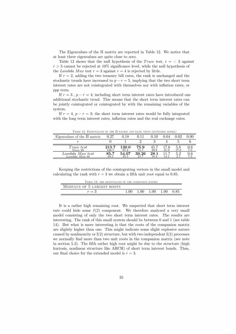
The Eigenvalues of the ¦ matrix are reported in Table 12. We notice thatat least three eigenvalues are quite close to zero.
Table 12 shows that the null hypothesis of the Trace test, r = < 3 againstr > 3 cannot be rejected at 10% signi…cance level, while the null hypothesis ofthe Lambda Max test r = 3 against r = 4 is rejected by little.
If r = 2, adding the two treasury bill rates, the rank is unchanged and thestochastic trends have increased to p ¡ r = 5, implying that the two short terminterest rates are not cointegrated with themselves nor with in‡ation rates, orppp term.
If r = 3 , p ¡ r = 4; including short term interest rates have introduced oneadditional stochastic trend. This means that the short term interest rates canbe jointly cointegrated or cointegrated by with the remaining variables of thesystem.
If r = 4, p ¡ r = 3; the short term interest rates would be fully integratedwith the long term interest rates, in‡ation rates and the real exchange rates.
Table 12: Eigenvalues of the ¦ matrix and rank tests (extended model)
Eigenvalues of the ¦ matrix 0:27 0:18 0:11 0:10 0:04 0:02 0:00r 0 1 2 3 4 5 6
Trace testTrace 90
215:7126:7
130:097:2
75:971:7
45:749:9
17:631:9
5:817:8
0:67:5
Lambda Max testLambda Max 90
85.729:5
54.0725:5
30.2621:7
28:118:3
11:714:1
5:22:1
0:67:5
Keeping the restrictions of the cointegrating vectors in the small model andcalculating the rank with r = 3 we obtain a …fth unit root equal to 0:85.
Table 13: the eigenvalues of the companion matrix
Modulus of 5 largest rootsr = 3 1:00 1:00 1:00 1:00 0:85
It is a rather high remaining root. We suspected that short term interestrate could hide some I(2) component. We therefore analysed a very smallmodel consisting of only the two short term interest rates. The results areinteresting. The rank of this small system should be between 0 and 1 (see table14). But what is more interesting is that the roots of the companion matrixare slightly higher than one. This might indicate some slight explosive naturecaused by nonlinearity or I(2) structure, but with two independent I(2) processeswe normally …nd more than two unit roots in the companion matrix (see notein section 5.2). The …fth rather high root might be due to the structure (highkurtosis, nonlinear structure like ARCH) of short term interest bonds. Thus,our …nal choice for the extended model is r = 3.
35

Table 14: Eigenvalues of the ¦ matrixand rank tests for short term interest rates
Eigenvalues of the ¦ matrix 0:05 0:2r 0 1
Trace testTrace 90
17:717:8
5:27:5
Lambda Max testLambda Max 90
12:510:3
5:27:5
Modulus of 2 largest rootsr unrestricted 1:0047 1:0047
6.3 Structural hypothesis test
An advantage of the principle of the ”speci…c to general” approach is that wecan keep the two cointrating relations found in the previous section unaltered.Hence the additional impact of the two new variables, the short term interestrates, should be described by a third cointegrating relation.
To obtain information about the new cointegrating relation we …rst estimatethe partially restricted long run structure keeping two cointegration relationunchanged (H3 and H16) but leaving unrestricted the third one (H17). Thehypothesis was accepted with a p ¡ value of 0:19, and the third cointegratingrelation suggested that it could contain information about the spread betweenlong and short interest rates in the two countries (table 15).
Table 15: The third unrestricted cointegrating relation
¢pt ¢p¤t ilt il¤t ist is
¤t pppt constant Â2 (º) p ¡ val
H17 0:617 ¡0:626 0:617 ¡0:894 ¡0:614 1:000 0:268 0:002 11:2 0:19
This led to test the following restricted hypothesis H18 that was acceptedwith a p ¡ value of 0:32:
Table 16: The third restricted cointegrating relation
¢pt ¢p¤t ilt il¤t ist is
¤t pppt constant Â2 (º) p ¡ val
H18 0:317 ¡0:317 0:317 ¡1 ¡0:317 1 0 0:001 12:6 0:32
The third vector can be written as:
(¢pt ¡ ¢p¤t ) +
¡ilt ¡ ist
¢¡ 3:15
³il¤t ¡ is
¤t
´s I(0) (19)
that relates the spread between prices with the spread of between interestrates.
In table 17 a structural representation of the cointegration space is …nallygiven. The adjustment coe¢cients are also reported. It is noticeable that none
36

of the adjustment parameters referring to ppp are signi…cant, suggesting thatppp is weakly exogenous variables. Some of the adjustment parameters aresigni…cant for the interest rates, but their absolute values are very close to zero.
Table 17: A structural representation of the cointegration space (extended model)^¯1
^¯2
^¯3
^®1
^®2
^®3
¢pt 1 ¡1 0:317 ¢2pt ¡0:53¡7:7
0:203:2
0:503:1
¢p¤t 0 1 ¡0:317 ¢2p¤
t ¡0:20¡1:5
¡0:33¡2:8
0:321:1
ilt ¡1 1 0:317 ¢ilt 0:001:1
0:012:3
0:032:8
il¤t 0 ¡1 ¡1 ¢il¤t 0:001:2
0:023:8
0:052:8
ist 0 0 ¡0:317 ist 0:000:9
0:010:7
0:054:1
is¤t 0 0 1 is¤
t 0:023:2
0:001:3
0:01¡0:5
ppp1t 0 ¡1 0 ¢pppt ¡0:01
¡1:50:000:2
0:00¡0:2
constant 0:004 ¡0:005 0:0011 The ppp term has been divided by 100
6.4 Common trends
As was shown in sections 5.3 and 5.6, there is a close relationship between longrun weak exogeneity and common trends. In section 5.6 it was shown that theweakly exogenous variables were the ones that generated the common trendsthat a¤ected all the variables in the system.
The long run weak exogeneity test is formulated as a zero row in ® and thenull hypothesis is that the variable is weakly exogenous. If the null hypothesisis accepted, the variable pushes the system. From table 17 we have some ideaabout which variables are not weakly exogenous, but it is more di¢cult to choosethe one between interest rates that has to be excluded to be a common trend.In fact we set r = 3, so we expect that p ¡ r = 7 ¡ 3 = 4 common trends.
We tested which variable was weakly exogenous setting a zero row in ® foreach variables (table 18). Table 18 shows that the short term interest rate inthe US is very unlikely weakly exogenous.
Table 18: tests for weak exogeneity
ilt il¤t ist is¤
t pppt
Â2 (3) 4:68 7:63 1:36 15:35 3:68p ¡ value 0:18 0:05 0:71 0:00 0:30
Lastly, in table 19 we report the VMA (common trends) representation basedon the fully speci…ed cointegrating relations with weak exogeneity of ilt, il¤t ; istand pppt imposed on ®.
The estimates of the C matrix in table 10 measure the total impact ofpermanent shocks to each of the variables on all other variables. A row of the Cmatrix gives an indication of which variables have been particularly importantfor the stochastic trend behaviour of the variable in the row.
37

Table 19: The estimates of the long run impact matrix C
CP ^
"ilt
P ^"il¤
t
P ^"is
t
P ^"pppt
¢pt 1.373:82
0:390:90
0:080:23
¡0:03¡0:18
¢p¤t 0:24
0:481:121:82
0:250:49
0.973:71
ilt 1.373:82
0:390:90
0:080:23
¡0:03¡0:18
il¤t 0:14¡0:35
1.202:75
0:170:43
0:080:41
ist 0:651:54
0:440:86
1.283:03
¡0:14¡0:65
is¤t -1.16
¡2:281.632:63
0:931:82
0:421:58
pppt 0:380:87
¡0:08¡0:15
0:080:19
0.9410:78
2666666664
¢pt
¢p¤t
iltil
¤t
istis
¤t
pppt
3777777775
=
2666666664
c11 0 0 00 0 0 c24
c11 0 0 00 c42 0 00 0 c53 0
c61 c62 0 00 0 0 c74
3777777775
2664
P"il
tP"il¤
tP"is
tP"pppt
3775 +
stationary anddeterministiccomponents
(20)
The …ndings from the restricted VMA representation suggest that (see rela-tion 20):
- German in‡ation rate and the long bond interest rate share the samestochastic trend. Real long term interest rates are constant in Germany.
- Shocks to the German long term interest rate speed up the German in‡ationand to some extent changes the ppp (via exchange rates as theory suggests).
- Shocks to the US long term interest pushes the US short interest rate as ifthe FED adjusts responds to the capital markets rather than anticipating them.
- Shocks to ppp coming from exchange rates have signi…cant e¤ects on theUS in‡ation proably because the US are not only a big exporter but also a bigimporter.
6.5 The role of short-term interest rate
To gain a further perspective on the role of the short relative to the long terminterest rate we report in Table 8 a comparative analysis of the combined e¤ect
measured by^¦r =
^®r
^¯
0, where the subscript r stands for the restricted estimates
as reported in table 9 and 17. It seems that short term interest rates weresigni…cantly important for the in‡ation rates in Germany, but not for the US.However if we have a close look table 19, it seems that short term interest ratedo not have permanent e¤ects on prices. Conversely, US in‡ation adjusts (table20) and are a¤ected in the long (table 19) run by shocks in pppt. All the other
38

variables, either because the t ¡ values are too small or the absolute value ofthe impact is very close to zero, seem not to be strongly a¤ected by any othervariables (table 19) but in the long run these small e¤ects have a tendency tocumulate (table 20).
Table 20:The combined long run effect^¦r=
^®r
^¯
0r
¢pt ¢p¤t ilt il¤t pppt
¢2pt ¡0:42¡5:7
¡0:020:5
0:425:7
¡0:02¡0:5
¡0:02¡0:5
¢2p¤t 0:37
2:7¡0:56
¡7:2¡0:37
¡2:70:567:2
0:567:2
¢ilt 0:000:4
0:001:9
-0:00¡0:4
¡0:00¡1:9
-0:00¡1:9
¢il¤t ¡0:00¡0:6
0:012:8
0:000:6
¡0:01¡2:8
¡0:01¡2:8
pppt ¡0:02¡1:9
0:000:3
0:021:9
¡0:00¡0:4
¡0:00¡0:4
¢pt ¢p¤t ilt il¤t pppt ist is¤
t
¢2pt ¡0:57¡7:4
0:040:8
0:886:5
¡0:69¡3:3
¡0:20¡3:2
¡0:16¡3:1
0:493:1
¢2p¤t 0:23
1:6¡0:43
¡5:3¡0:03¡0:1
0:000:0
0:322:8
¡0:10¡1:0
0:321:0
¢ilt 0:011:0
¡0:00¡0:0
0:011:5
¡0:05¡2:9
¡0:01¡2:3
¡0:01¡2:8
0:032:8
¢il¤t ¡0:01¡1:0
0:012:1
0:042:7
¡0:08¡3:3
¡0:03¡3:8
¡0:02¡2:8
0:052:8
pppt ¡0:02¡1:7
0:040:5
0:020:8
0:000:1
0:00¡0:2
0:000:2
¡0:01¡0:2
¢ist 0:011:5
0:002:5
¡0:02¡1:3
¡0:060:0
¡0:01¡1:3
0:000:5
¡0:01¡0:5
¢is¤t ¡0:01
¡1:70:010:6
0:020:8
0:000:1
¡0:0¡0:2
¡0:000:2
¡0:01¡0:2
7 ConclusionsTwo building blocks of international monetary economics are the ppp and uipconditions. They are normally assumed stationary, i.e. I(0). Recently it was dis-covered that ppp and uip are not stationary at all, but they do behave like mostof the economic time series. Basically they move like random walk, that is theyare I(1). This fact has been represented just an enigma for many economists.
Juselius (1995) and Juselius and MacDonald (2000), exploiting the I(1) prop-erty of the ppp and uip, put forward the idea that ppp and uip were linkedtogether producing a stationary relationship. Just because ppp and uip wereI(1), they could produce a stationary relationship like uip ¡ ppp s I(0).
This paper provided evidence that the cointegrating international parityrelationships discovered by Juselius and MacDonald hold also in the case weused a di¤erent price index measure. This result is quite interesting since thewholesale price index we used, was not directly cointegrated (section 3.2.1) withthe CPI index used by Juselius and MacDonald.
39

We found that the fundamental relation that combines the ppp with theuip (ilt ¡ il¤t ) ¡ !1(¢pt ¡ ¢p¤
t ) ¡ !2pppt s I(0), consistent with a world inwhich rational and chartists agents (section 2.3) coexist, was accepted with avery high p ¡ value; but the more interesting result was that the estimatedcoe¢cients !1 and !2 were very close to one (H14 section 5.4), i.e. very close toa world dominated by rational agents (section 2.3). We therefore tested whethera particular restriction to this model could be accepted: we tested the modelimposing !1 and !2 equal to one. This theoretical case, in which fully rationalagents were allowed, was strongly accepted (H16)!
We found also another interesting cointegration relation: real interest ratesare stationary in Germany (H3)! Jointly tested H16 and H3 were accepted withvery high p-values.
These results were also con…rmed in the extended model which includedshort term interest rates (H18, section 6.3): the same hypothesis were acceptedand another interesting cointegrating relation between the spread of interestrates was found (section 6.3 equation (19)).
ReferencesE. Colombo and Lossani M., 2000, Economia Monetaria Internazionale, Uni-
versita’ Cattolica Milano.W Enders, 1995, Applied Econometric Time Series, John Wiley & Sons,
New York.H. Hansen and Juselius K., 2000, CATS in RATS: Cointegration Analysis
of Time Series, Estima, Evanston.P.R. Hansen and Johansen S . , 1998, Workbook on Cointegration, Oxford
University Press.S. Johansen and Juselius K., 1994, Identi…cation of the long-run and the
short-run structure: an application to the ISLM model, Journal of Economet-rics, pp. 7-36.
K. Juselius, 1995, ”Do purchasing power parity and uncovered interest rateparity hold in the long run? An example of likelihood inference in a multivariatetime-series model”, Journal of Econometrics, pp. 211-240.
K. Juselius and MacDonald R., 2000, ”International parity relationshipsbetween Germany and the United States: a joint modelling approach”, forth-coming.
K Rogo¤, 1996, ”The purchasing power parity puzzle”, Journal of EconomicsLiterature, pp. 647-668.
40