International School on Applications with the

Newest Multi-spectral Environmental Satellites

held in Brienza from 18 to 24 Sep 2011

Paul Menzel, Valerio Tramutoli, & Filomena Romana

2

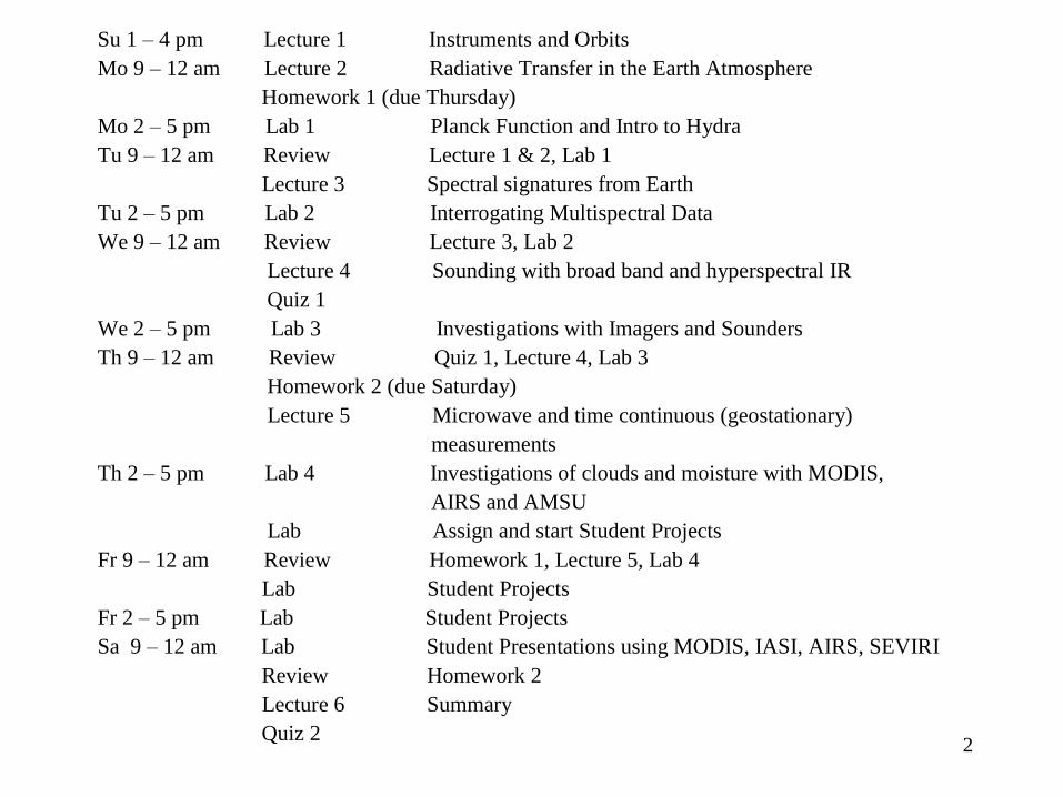
Su 1 – 4 pm Lecture 1 Instruments and Orbits

Mo 9 – 12 am Lecture 2 Radiative Transfer in the Earth Atmosphere

Homework 1 (due Thursday)

Mo 2 – 5 pm Lab 1 Planck Function and Intro to Hydra

Tu 9 – 12 am Review Lecture 1 & 2, Lab 1

Lecture 3 Spectral signatures from Earth

Tu 2 – 5 pm Lab 2 Interrogating Multispectral Data

We 9 – 12 am Review Lecture 3, Lab 2

Lecture 4 Sounding with broad band and hyperspectral IR

Quiz 1

We 2 – 5 pm Lab 3 Investigations with Imagers and Sounders

Th 9 – 12 am Review Quiz 1, Lecture 4, Lab 3

Homework 2 (due Saturday)

Lecture 5 Microwave and time continuous (geostationary)

measurements

Th 2 – 5 pm Lab 4 Investigations of clouds and moisture with MODIS,

AIRS and AMSU

Lab Assign and start Student Projects

Fr 9 – 12 am Review Homework 1, Lecture 5, Lab 4

Lab Student Projects

Fr 2 – 5 pm Lab Student Projects

Sa 9 – 12 am Lab Student Presentations using MODIS, IASI, AIRS, SEVIRI

Review Homework 2

Lecture 6 Summary

Quiz 2

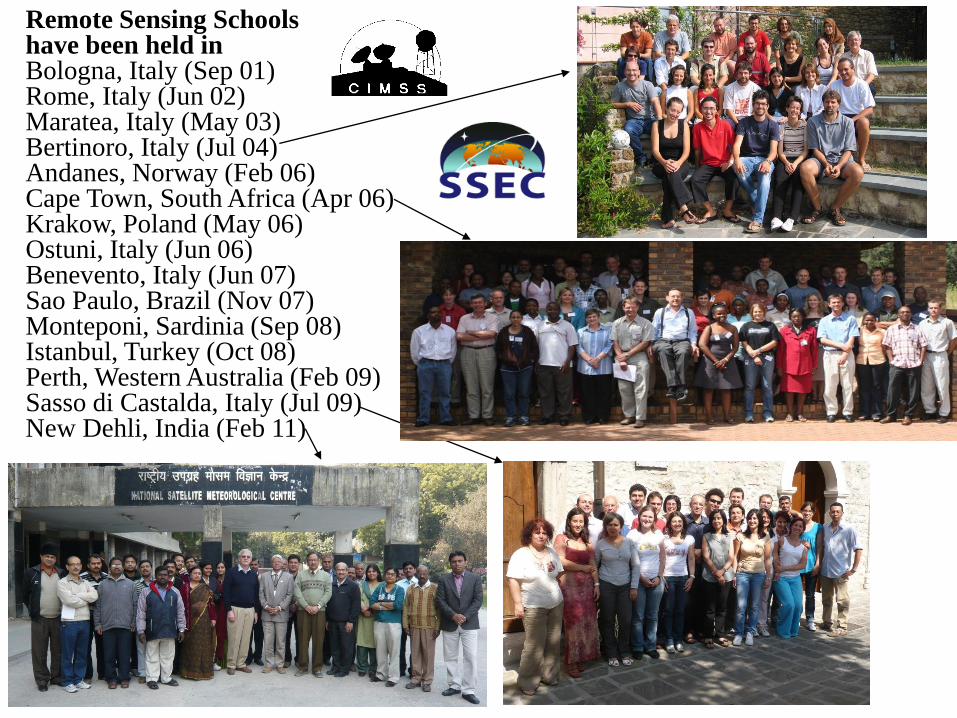
Remote Sensing Schools have been held in Bologna, Italy (Sep 01) Rome, Italy (Jun 02) Maratea, Italy (May 03) Bertinoro, Italy (Jul 04) Andanes, Norway (Feb 06) Cape Town, South Africa (Apr 06) Krakow, Poland (May 06) Ostuni, Italy (Jun 06) Benevento, Italy (Jun 07) Sao Paulo, Brazil (Nov 07) Monteponi, Sardinia (Sep 08) Istanbul, Turkey (Oct 08) Perth, Western Australia (Feb 09) Sasso di Castalda, Italy (Jul 09) New Dehli, India (Feb 11)

Objective of School

An in depth explanation of methods and techniques

used to extract information from environmental

satellite data, with emphasis on the latest

measuring technologies. The course will consist of

lectures, laboratory sessions, group lab projects,

homework and tests. The results from each of the

group projects will be presented to the class by the

participating students. English is the official

language of the School. All provided material will

be in English. 4

Lectures and Labs

Lectures and laboratory exercises emphasize investigation of high spatial resolution visible and

infrared data (from MODIS and SEVIRI), high spectral resolution infrared data (from AIRS and

IASI), and microwave sounding data (AMSU). Text for the classroom and a visualization tool for

the labs are provided free; “Applications with Meteorological Satellites” is used as a resource text

from ftp://ftp.ssec.wisc.edu/pub/menzel/ and HYDRA is used to interrogate and view multispectral

data in the labs from http://www.ssec.wisc.edu/hydra/. Homework assignments and classroom tests

are administered to verify that good progress is being was made in learning and mastering the

materials presented. Classroom size is usually between twenty and thirty students.

5

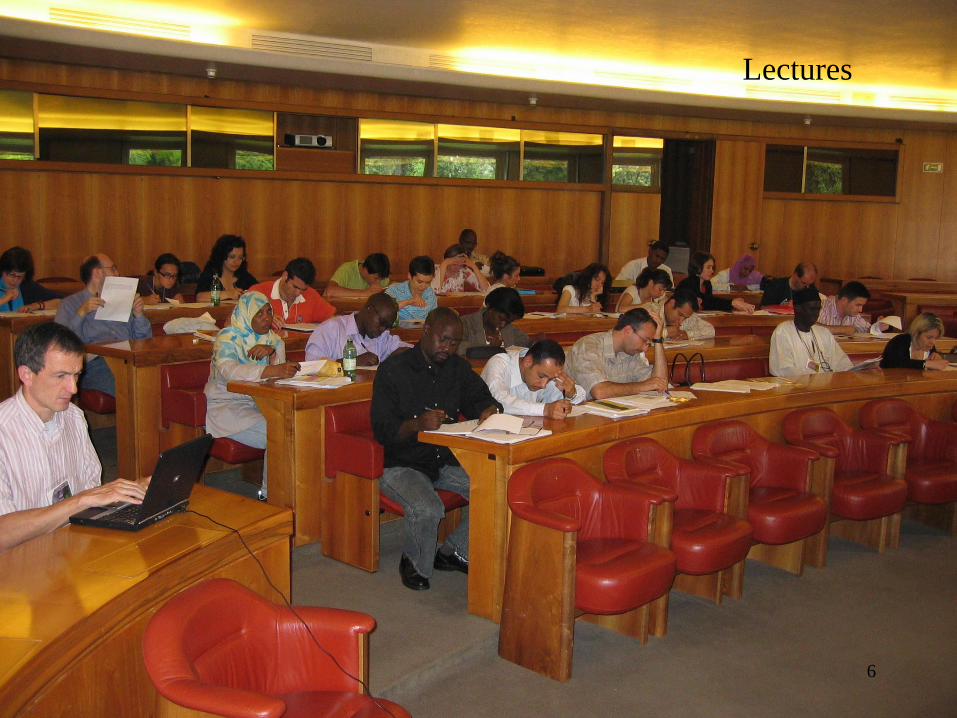
Lectures

6

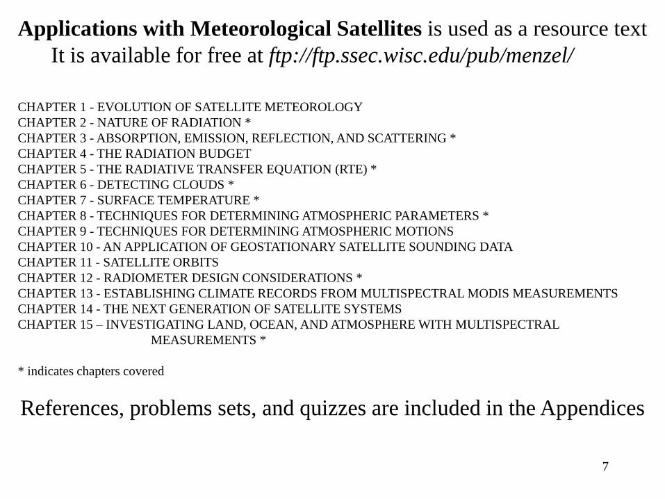
Applications with Meteorological Satellites is used as a resource text

It is available for free at ftp://ftp.ssec.wisc.edu/pub/menzel/

CHAPTER 1 - EVOLUTION OF SATELLITE METEOROLOGY

CHAPTER 2 - NATURE OF RADIATION *

CHAPTER 3 - ABSORPTION, EMISSION, REFLECTION, AND SCATTERING *

CHAPTER 4 - THE RADIATION BUDGET

CHAPTER 5 - THE RADIATIVE TRANSFER EQUATION (RTE) *

CHAPTER 6 - DETECTING CLOUDS *

CHAPTER 7 - SURFACE TEMPERATURE *

CHAPTER 8 - TECHNIQUES FOR DETERMINING ATMOSPHERIC PARAMETERS *

CHAPTER 9 - TECHNIQUES FOR DETERMINING ATMOSPHERIC MOTIONS

CHAPTER 10 - AN APPLICATION OF GEOSTATIONARY SATELLITE SOUNDING DATA

CHAPTER 11 - SATELLITE ORBITS

CHAPTER 12 - RADIOMETER DESIGN CONSIDERATIONS *

CHAPTER 13 - ESTABLISHING CLIMATE RECORDS FROM MULTISPECTRAL MODIS MEASUREMENTS

CHAPTER 14 - THE NEXT GENERATION OF SATELLITE SYSTEMS

CHAPTER 15 – INVESTIGATING LAND, OCEAN, AND ATMOSPHERE WITH MULTISPECTRAL

MEASUREMENTS *

* indicates chapters covered

References, problems sets, and quizzes are included in the Appendices

7

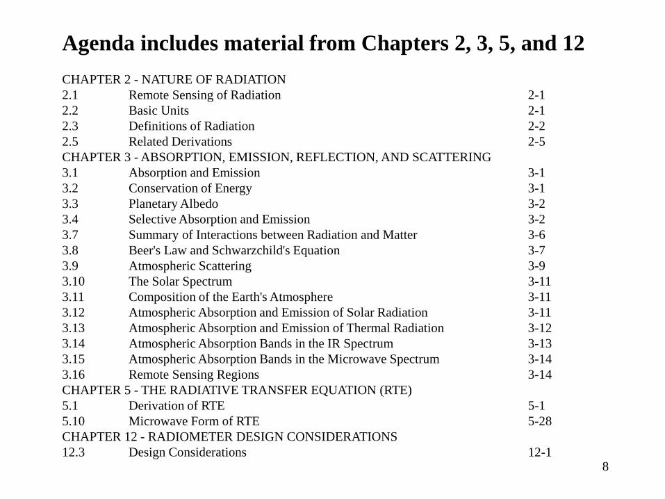
Agenda includes material from Chapters 2, 3, 5, and 12

CHAPTER 2 - NATURE OF RADIATION

2.1 Remote Sensing of Radiation 2-1

2.2 Basic Units 2-1

2.3 Definitions of Radiation 2-2

2.5 Related Derivations 2-5

CHAPTER 3 - ABSORPTION, EMISSION, REFLECTION, AND SCATTERING

3.1 Absorption and Emission 3-1

3.2 Conservation of Energy 3-1

3.3 Planetary Albedo 3-2

3.4 Selective Absorption and Emission 3-2

3.7 Summary of Interactions between Radiation and Matter 3-6

3.8 Beer's Law and Schwarzchild's Equation 3-7

3.9 Atmospheric Scattering 3-9

3.10 The Solar Spectrum 3-11

3.11 Composition of the Earth's Atmosphere 3-11

3.12 Atmospheric Absorption and Emission of Solar Radiation 3-11

3.13 Atmospheric Absorption and Emission of Thermal Radiation 3-12

3.14 Atmospheric Absorption Bands in the IR Spectrum 3-13

3.15 Atmospheric Absorption Bands in the Microwave Spectrum 3-14

3.16 Remote Sensing Regions 3-14

CHAPTER 5 - THE RADIATIVE TRANSFER EQUATION (RTE)

5.1 Derivation of RTE 5-1

5.10 Microwave Form of RTE 5-28

CHAPTER 12 - RADIOMETER DESIGN CONSIDERATIONS

12.3 Design Considerations 12-1

8

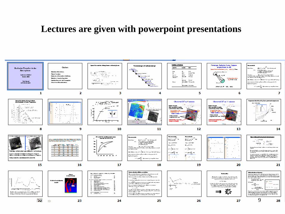
Lectures are given with powerpoint presentations

9

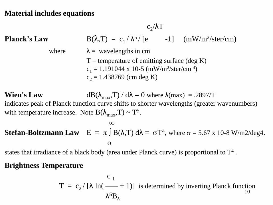
Material includes equations

c2/λT

Planck’s Law B(λ,T) = c1 / λ5 / [e -1] (mW/m2/ster/cm)

where λ = wavelengths in cm

T = temperature of emitting surface (deg K)

c1 = 1.191044 x 10-5 (mW/m2/ster/cm-4)

c2 = 1.438769 (cm deg K)

Wien's Law dB(λmax,T) / dλ = 0 where λ(max) = .2897/T

indicates peak of Planck function curve shifts to shorter wavelengths (greater wavenumbers)

with temperature increase. Note B(λmax,T) ~ T5.

Stefan-Boltzmann Law E = B(λ,T) dλ = T4, where = 5.67 x 10-8 W/m2/deg4.

o

states that irradiance of a black body (area under Planck curve) is proportional to T4 . Brightness Temperature

c 1

T = c2 / [λ ln( _____ + 1)] is determined by inverting Planck function

λ5Bλ

10

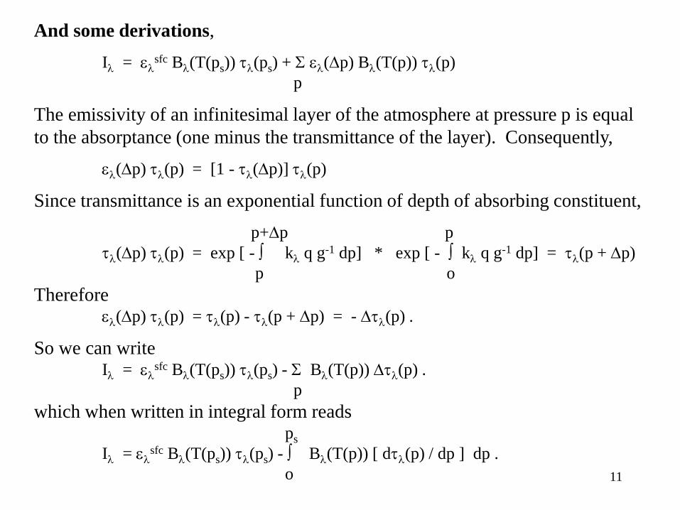
And some derivations, I =

sfc B(T(ps)) (ps) + (p) B(T(p)) (p)

p

The emissivity of an infinitesimal layer of the atmosphere at pressure p is equal

to the absorptance (one minus the transmittance of the layer). Consequently, (p) (p) = [1 - (p)] (p)

Since transmittance is an exponential function of depth of absorbing constituent, p+p p

(p) (p) = exp [ - k q g-1 dp] * exp [ - k q g-1 dp] = (p + p)

p o

Therefore (p) (p) = (p) - (p + p) = - (p) .

So we can write I =

sfc B(T(ps)) (ps) - B(T(p)) (p) .

p

which when written in integral form reads ps

I = sfc B(T(ps)) (ps) - B(T(p)) [ d(p) / dp ] dp .

o 11

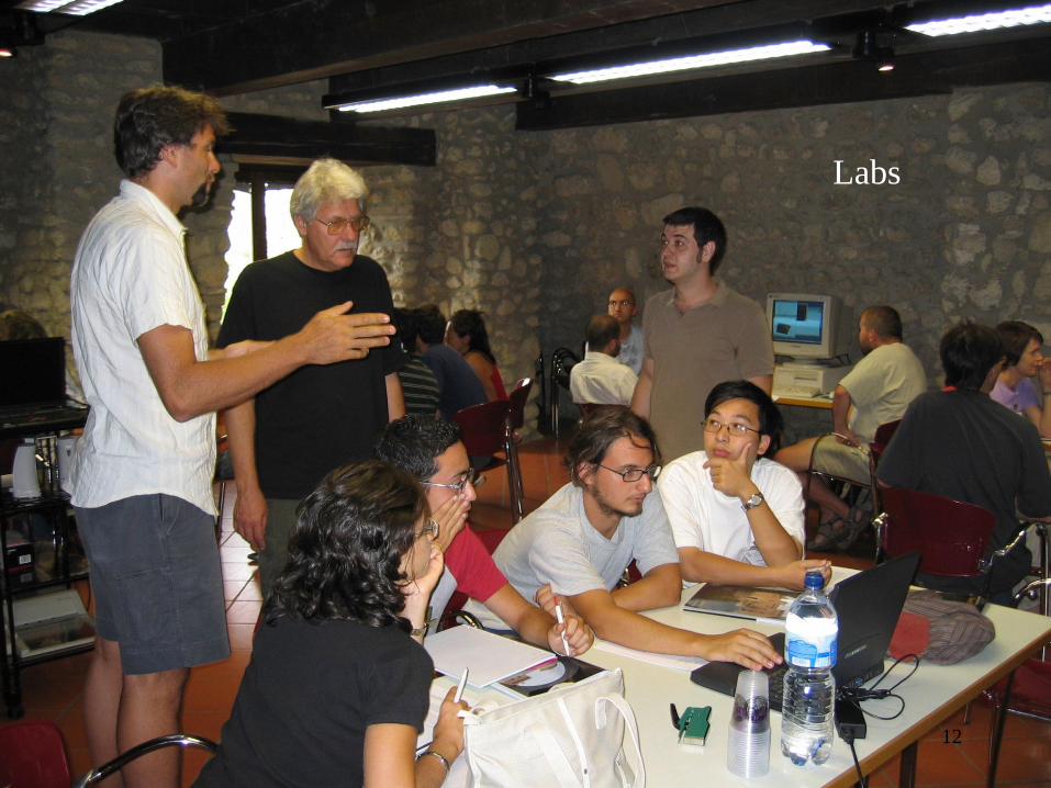
Labs

12

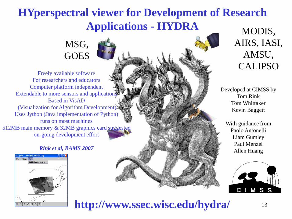
HYperspectral viewer for Development of Research

Applications - HYDRA

http://www.ssec.wisc.edu/hydra/

MSG,

GOES

MODIS,

AIRS, IASI,

AMSU,

CALIPSO

Developed at CIMSS by

Tom Rink

Tom Whittaker

Kevin Baggett

With guidance from

Paolo Antonelli

Liam Gumley

Paul Menzel

Allen Huang

Freely available software

For researchers and educators

Computer platform independent

Extendable to more sensors and applications

Based in VisAD

(Visualization for Algorithm Development)

Uses Jython (Java implementation of Python)

runs on most machines

512MB main memory & 32MB graphics card suggested

on-going development effort

Rink et al, BAMS 2007

13

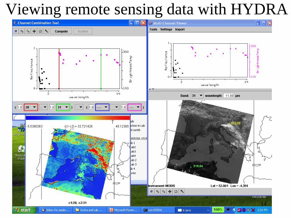
Viewing remote sensing data with HYDRA

14

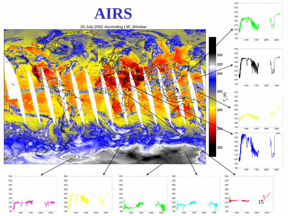
AIRS 20-July-2002 Ascending LW_Window

15

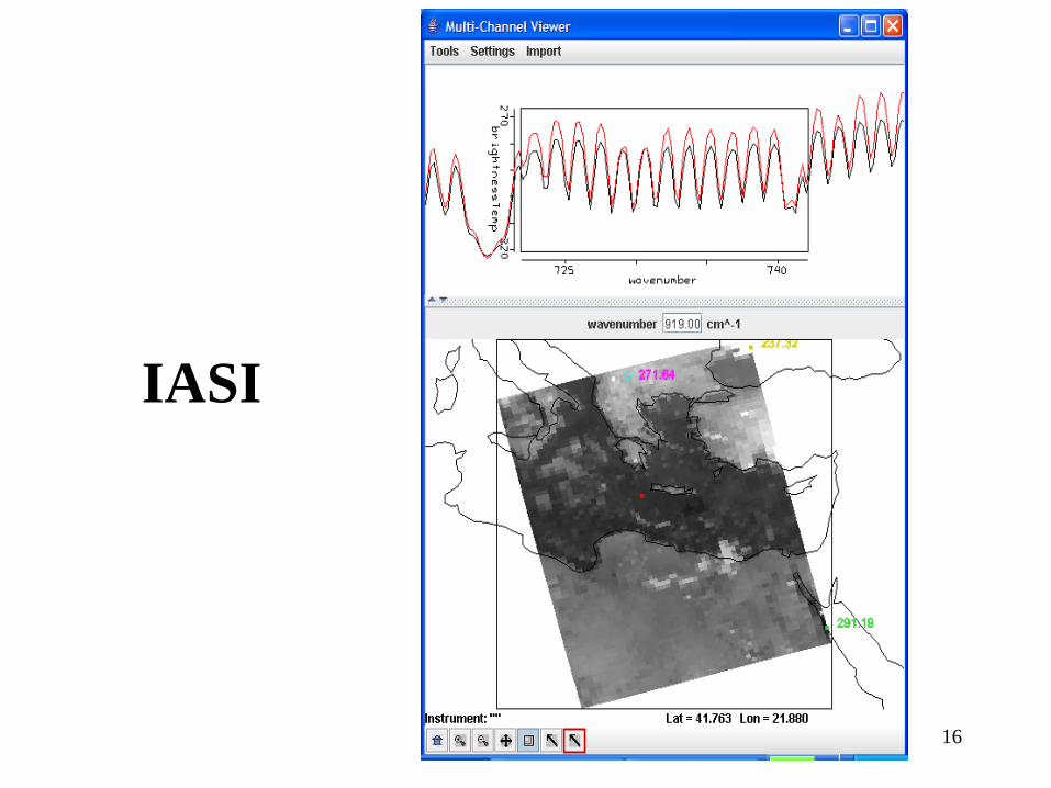
IASI

16

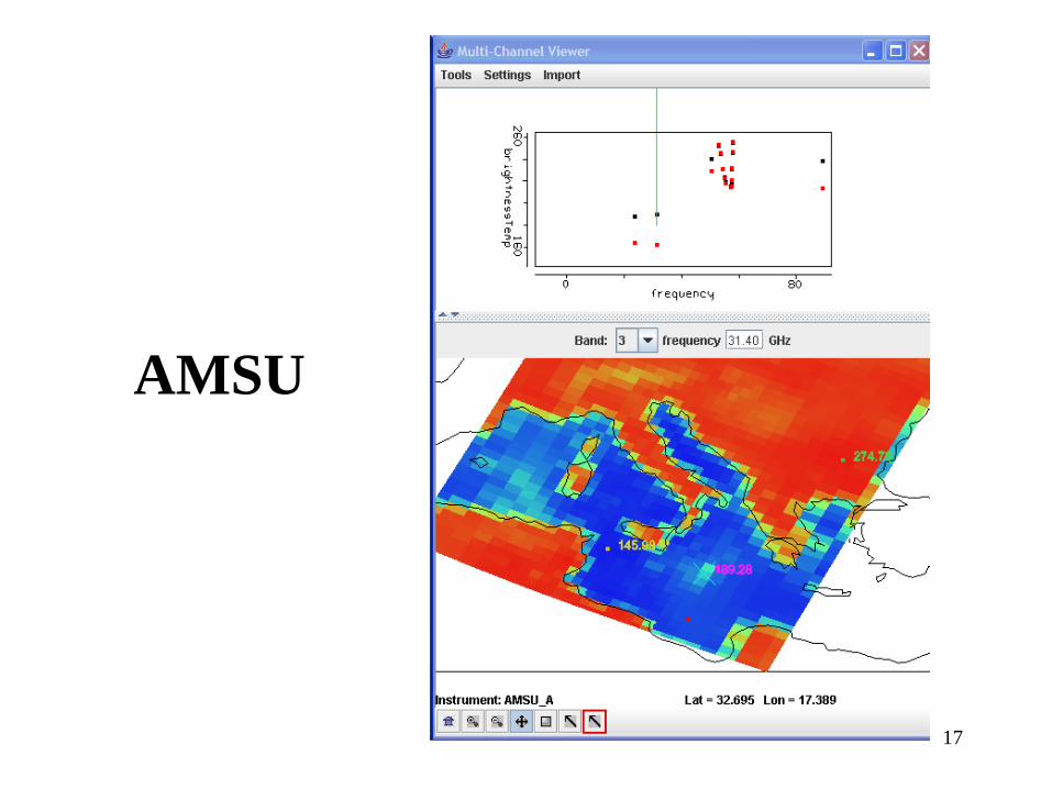
AMSU

17

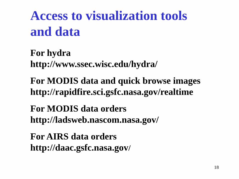
Access to visualization tools

and data For hydra

http://www.ssec.wisc.edu/hydra/

For MODIS data and quick browse images

http://rapidfire.sci.gsfc.nasa.gov/realtime For MODIS data orders

http://ladsweb.nascom.nasa.gov/ For AIRS data orders

http://daac.gsfc.nasa.gov/

18

Orbits and Instruments

Lectures in Brienza

18 Sep 2011

Paul Menzel

UW/CIMSS/AOS

20

All

Sats

on

NASA

J-track

http://science.nasa.gov/Realtime/jtrack/3d/JTrack3D.html 21

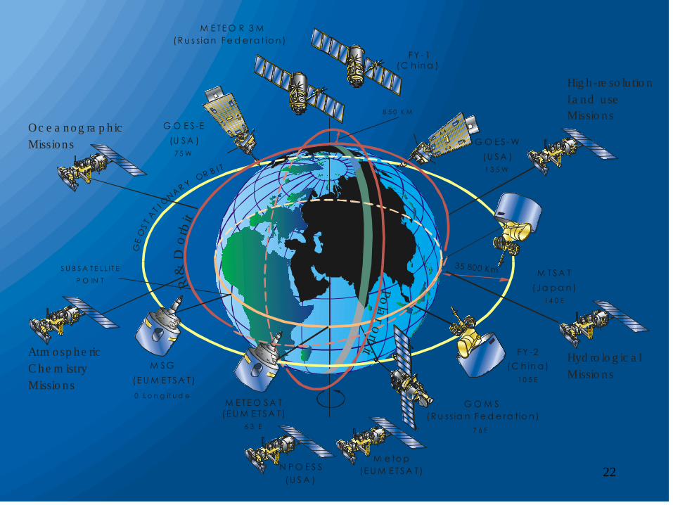
8 5 0 K M

35 800 KmS U B S A T E L L I T E

P O IN T

G O M S

(R u ss ia n F e d e ra tio n )

7 6 E

M S G

(E U M E T S A T )

6 3 E

M T S A T

( J a p a n )

1 4 0 E

F Y -2

(C h in a )

1 0 5 E

G O E S -E

(U S A )

7 5 W

N P O E S S

(U S A )

G O E S - W

(U S A )

1 3 5 W

GE

OS

TA

T

I ON

AR Y O

R B I T

Oc e a n o g ra p h ic

Missio n s

Atm o sp h e ric

C h e m istry

Missio n s

Hyd ro lo g ic a l

Missio n s

Hig h -re so lu tio n

La n d u se

Missio n s

M E T E O R 3 M

(R u s s ia n F e d e ra t io n )

Po

lar o

rbit

R &

D o

rbit

M E T E O S A T

(E U M E T S A T )

0 L o n g it u d e

(C h in a )F Y - 1

M e to p

(E U M E T S A T ) 22

23

24

25

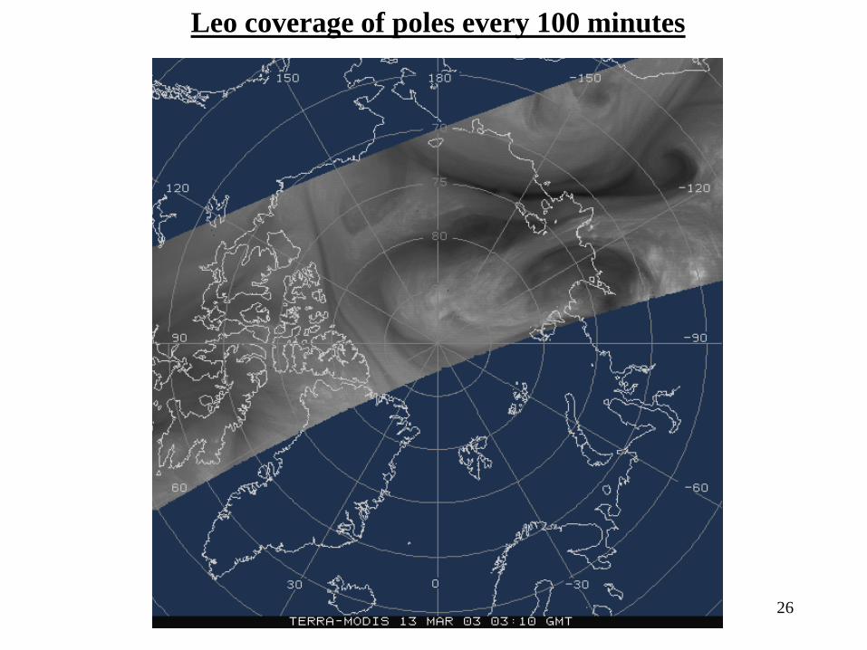
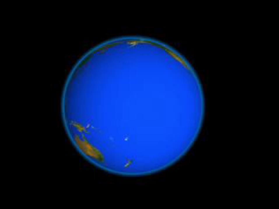
Leo coverage of poles every 100 minutes

26

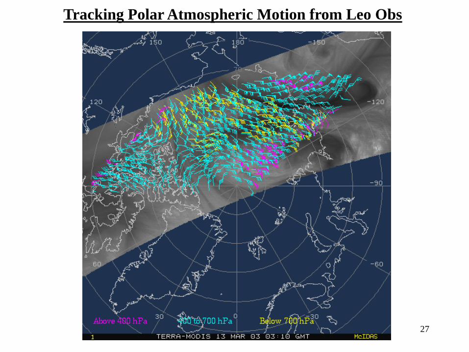
Tracking Polar Atmospheric Motion from Leo Obs

27

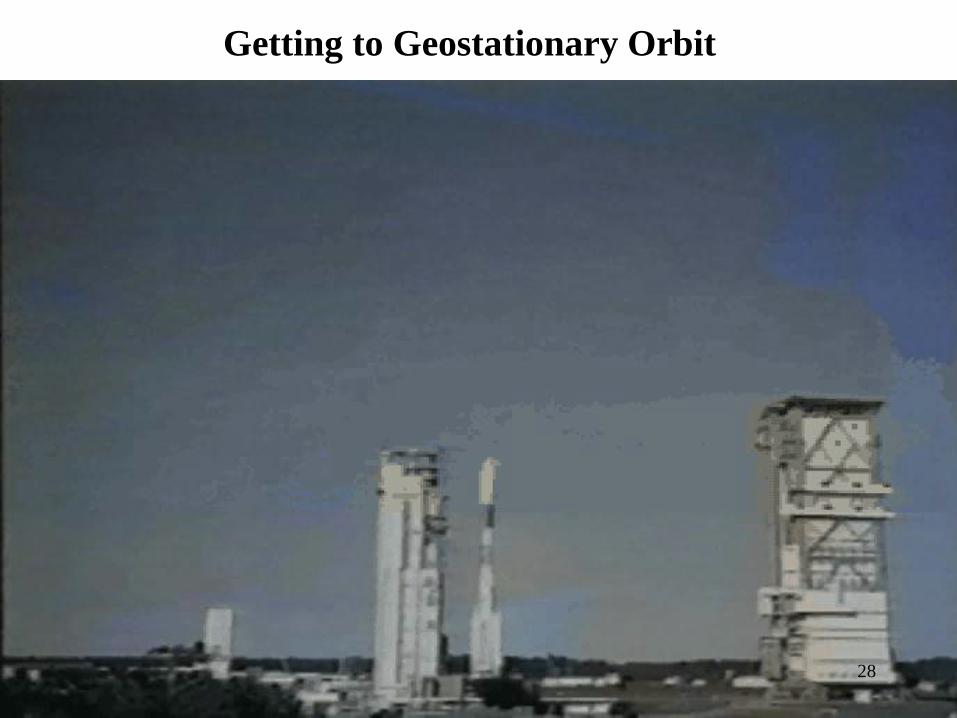
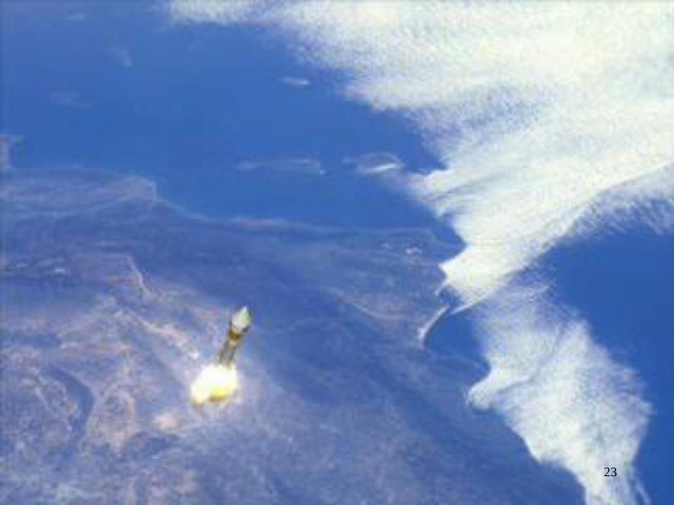
Getting to Geostationary Orbit

28

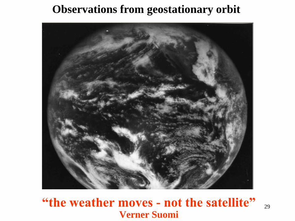
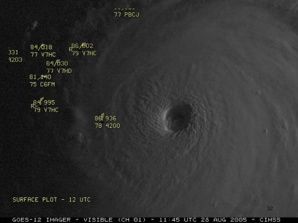
“the weather moves - not the satellite”

Verner Suomi

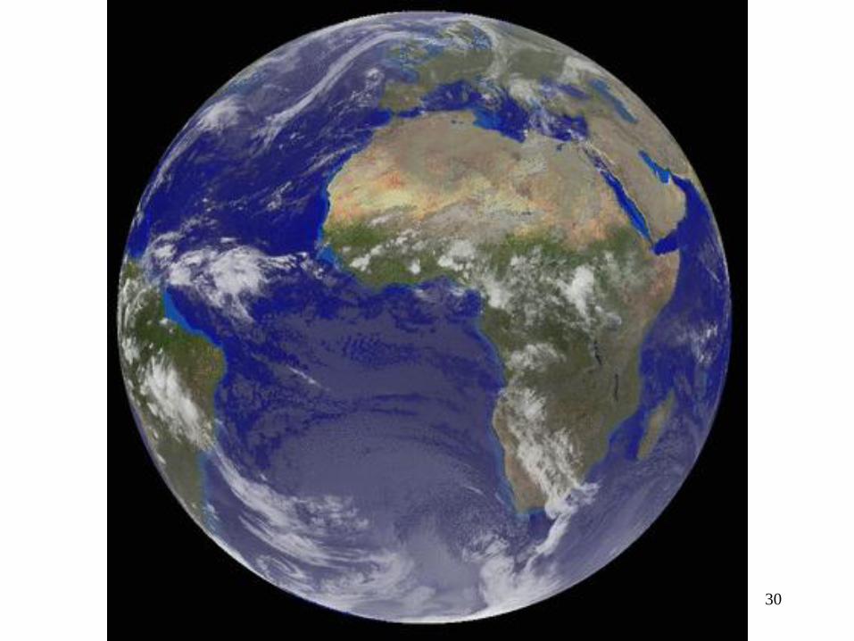
Observations from geostationary orbit

29

30

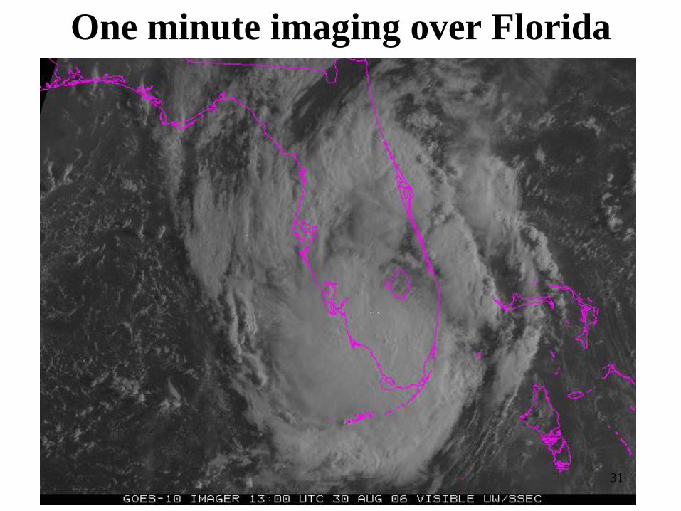
One minute imaging over Florida

31

32

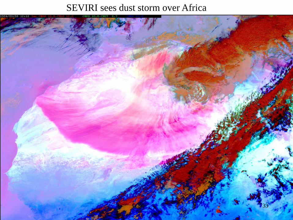
SEVIRI sees dust storm over Africa

33

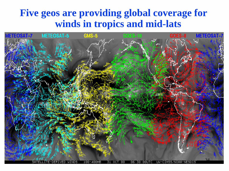
Five geos are providing global coverage for winds in tropics and mid-lats

34

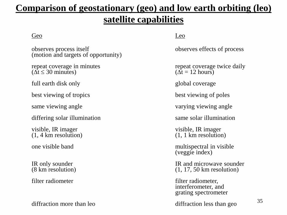
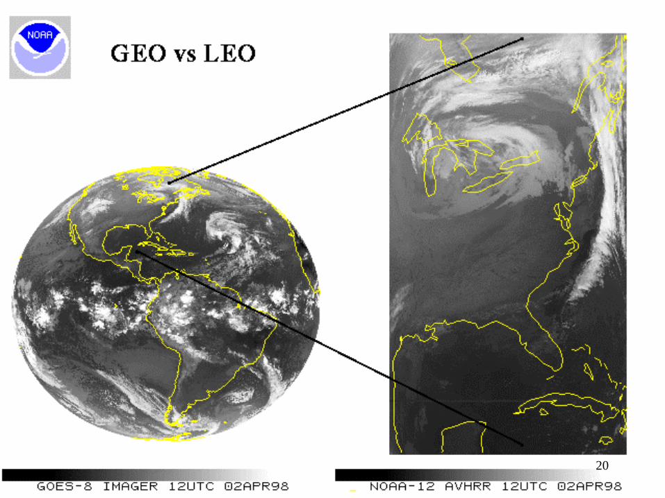
Comparison of geostationary (geo) and low earth orbiting (leo)

satellite capabilities

Geo Leo

observes process itself observes effects of process (motion and targets of opportunity) repeat coverage in minutes repeat coverage twice daily (t 30 minutes) (t = 12 hours) full earth disk only global coverage best viewing of tropics best viewing of poles same viewing angle varying viewing angle differing solar illumination same solar illumination visible, IR imager visible, IR imager (1, 4 km resolution) (1, 1 km resolution) one visible band multispectral in visible (veggie index) IR only sounder IR and microwave sounder (8 km resolution) (1, 17, 50 km resolution) filter radiometer filter radiometer, interferometer, and grating spectrometer

diffraction more than leo diffraction less than geo 35

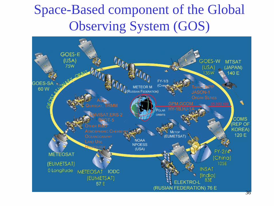
Space-Based component of the Global

Observing System (GOS)

36

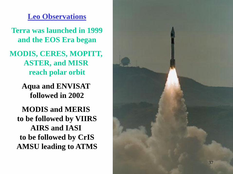
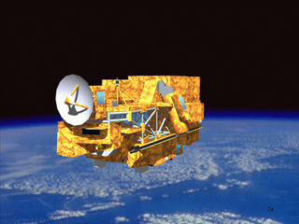
Leo Observations

Terra was launched in 1999

and the EOS Era began

MODIS, CERES, MOPITT,

ASTER, and MISR

reach polar orbit

Aqua and ENVISAT

followed in 2002

MODIS and MERIS

to be followed by VIIRS

AIRS and IASI

to be followed by CrIS

AMSU leading to ATMS

37

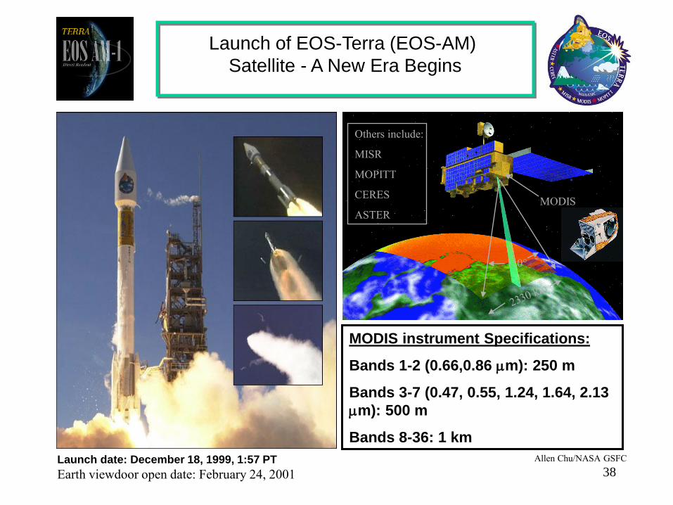
Launch of EOS-Terra (EOS-AM)�

Satellite - A New Era Begins

Launch date: December 18, 1999, 1:57 PT

Earth viewdoor open date: February 24, 2001

110°

MODIS

Others include:

MISR

MOPITT

CERES

ASTER

MODIS instrument Specifications:

Bands 1-2 (0.66,0.86 mm): 250 m

Bands 3-7 (0.47, 0.55, 1.24, 1.64, 2.13

mm): 500 m

Bands 8-36: 1 km

Allen Chu/NASA GSFC

38

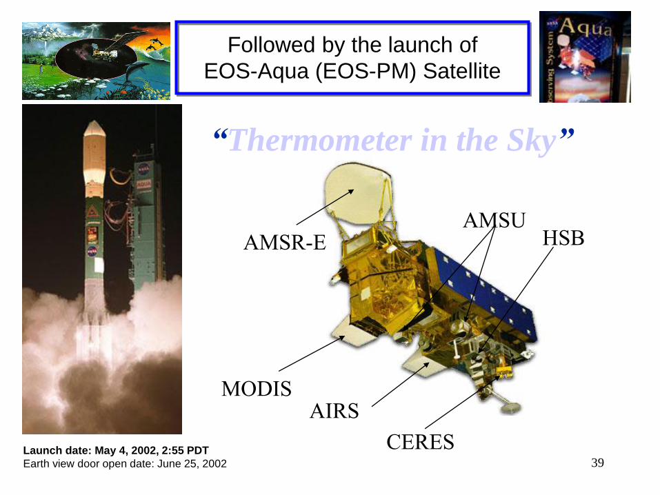
Followed by the launch of

EOS-Aqua (EOS-PM) Satellite

Launch date: May 4, 2002, 2:55 PDT

Earth view door open date: June 25, 2002

AIRS MODIS

AMSR-E AMSU

HSB

CERES

“Thermometer in the Sky”

39

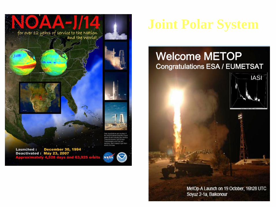
Welcome METOP Congratulations ESA / EUMETSAT

Joint Polar System

IASI

40

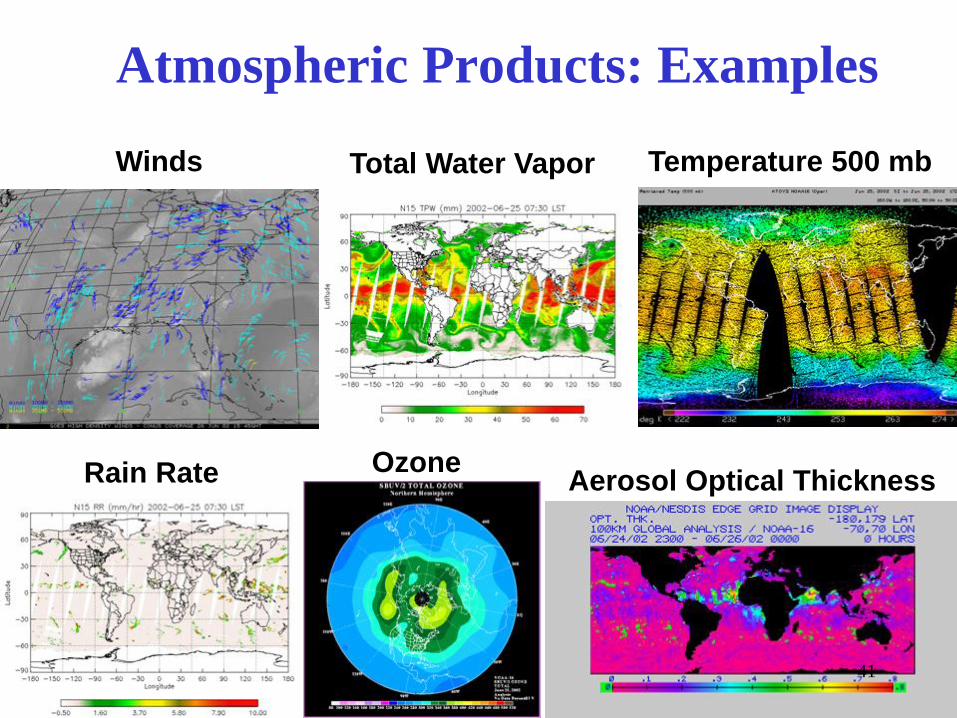
Atmospheric Products: Examples

Winds Total Water Vapor Temperature 500 mb

Rain Rate Ozone Aerosol Optical Thickness

41

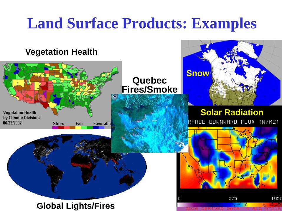
Land Surface Products: Examples

Vegetation Health

Snow

Solar Radiation

Quebec Fires/Smoke

Global Lights/Fires 42

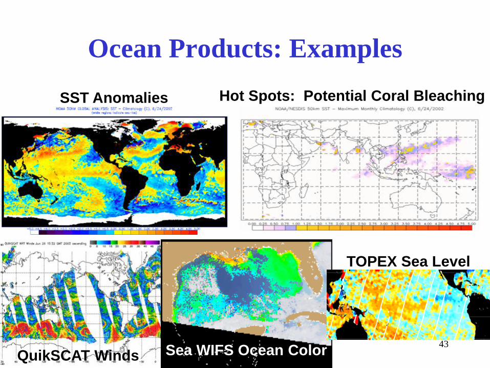
Ocean Products: Examples

SST Anomalies Hot Spots: Potential Coral Bleaching

QuikSCAT Winds Sea WIFS Ocean Color

TOPEX Sea Level

43

Remote Sensing Advantages

* provides a regional view * enables one to observe & measure the causes & effects of climate

& environmental changes (both natural & human-induced) * provides repetitive geo-referenced looks at the same area * covers a broader portion of the spectrum than the human eye * can focus in on a very specific bandwidth in an image * can also look at a number of bandwidths simultaneously * operates in all seasons, at night, and in bad weather

44

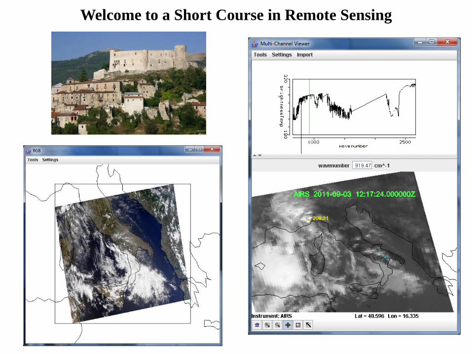
Welcome to a Short Course in Remote Sensing

45

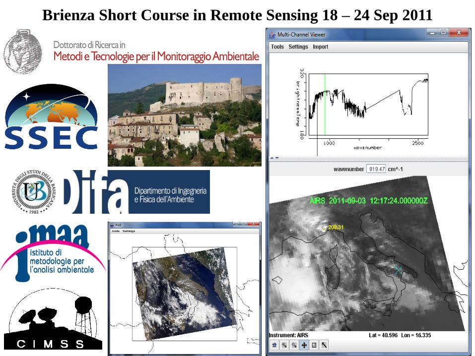
Brienza Short Course in Remote Sensing 18 – 24 Sep 2011

46